Detection and Tracking Using Particle-Filter-Based Wireless Sensor Networks

Detection and Tracking UsingParticle-Filter-Based Wireless Sensor Networks

Nadeem Ahmed, Member, IEEE, Mark Rutten, Travis Bessell, Salil S. Kanhere, Member, IEEE,

Neil Gordon, Member, IEEE, and Sanjay Jha, Senior Member, IEEE

Abstract—The work reported in this paper investigates the performance of the Particle Filter (PF) algorithm for tracking a moving

object using a wireless sensor network (WSN). It is well known that the PF is particularly well suited for use in target tracking

applications. However, a comprehensive analysis on the effect of various design and calibration parameters on the accuracy of the PF

has been overlooked. This paper outlines the results from such a study. In particular, we evaluate the effect of various design

parameters (such as the number of deployed nodes, number of generated particles, and sampling interval) and calibration parameters

(such as the gain, path loss factor, noise variations, and nonlinearity constant) on the tracking accuracy and computation time of the

particle-filter-based tracking system. Based on our analysis, we present recommendations on suitable values for these parameters,

which provide a reasonable trade-off between accuracy and complexity. We also analyze the theoretical Cramer-Rao Bound as the

benchmark for the best possible tracking performance and demonstrate that the results from our simulations closely match the

theoretical bound. In this paper, we also propose a novel technique for calibrating off-the-shelf sensor devices. We implement the

tracking system on a real sensor network and demonstrate its accuracy in detecting and tracking a moving object in a variety of

scenarios. To the best of our knowledge, this is the first time that empirical results from a PF-based tracking system with off-the-shelf

WSN devices have been reported. Finally, we also present simple albeit important building blocks that are essential for field

deployment of such a system.

Index Terms—Wireless sensor networks, simulations, experiments, performance attributes, measurements.

Ç

1 INTRODUCTION

WIRELESS Sensor Networks (WSN) are increasingly beingused in a variety of applications ranging from

environmental monitoring to industrial automation. Aparticularly promising military application involves usingWSN for detecting and tracking moving targets such astanks, vehicles, and troops. Detection and tracking of targetsis a mature and well-established research area. However,the current solutions rely on expensive and bulky sensors.The use of low-cost sensor nodes is an attractive andcomplementary approach.

Among several tracking algorithms in the literature that

use nonlinear filters, the Particle Filter (PF) [1] has been a

popular choice. The PF (also known as the sequential Monte

Carlo method) approximates a belief state for the presence

of the target by means of many but finite random samples.

Previous work [2], [3], [4] has demonstrated that the PF can

be effectively employed in WSN systems for tracking

applications. The tracking and detection performance of

such a system is significantly influenced by several design

parameters (such as number of sensors, number ofgenerated particles, and sampling frequency) and estima-tion of the calibration parameters (such as sensor gain, pathloss factor, noise, and nonlinearity constant). However, allprior work simply assumes a particular set of values forthese parameters without providing any insight into howthey affect the behavior of the tracking system. In thispaper, we conduct extensive simulations in a realisticenvironment to study the effect of the aforementionedparameters on the tracking and detection performance ofthe system.

We consider the problem of simultaneous detection andtracking of an object moving through a particular targetregion. In our system, sensor nodes equipped with acousticsensors are deployed in the target region. The sensorsperiodically sample the ambient sound and relay themeasured samples to a central base station. The movingobject generates an acoustic signature as it travels, which iscaptured by the acoustic measurements of the motes thatare located near the object. The base station runs the PFalgorithm on the collected samples, with the intensity of theobject’s acoustic signal acting as the input. The PF estimatesthe presence of the object and, if the object is declaredpresent, also estimates the object’s trajectory. In this work,we have conducted extensive simulations of this trackingsystem using NS2 to study the impact of various design andcalibration parameters on the tracking performance. Thetwo metrics that we have used to evaluate the performanceof the system are: track estimation error, i.e., the distancebetween the estimated and the actual location of the targetand computation time, i.e., the time required by the PF toexecute. Our simulation environment takes into account

1332 IEEE TRANSACTIONS ON MOBILE COMPUTING, VOL. 9, NO. 9, SEPTEMBER 2010

. N. Ahmed, S.S. Kanhere, and S. Jha are with the School of ComputerScience and Engineering, University of New South Wales, Building K17,Anzac Parade, Kensington, 2052 Sydney, Australia.E-mail: {nahmed, salilk, sanjay}@cse.unsw.edu.au.

. M. Rutten, T. Bessell, and N. Gordon are with the Defence Science andTechnology Organization (DSTO), 200 Labs, PO Box 1500, Edinburgh,SA 5111, Australia.E-mail: {mark.rutten, travis.bessell, neil.gordon}@dsto.defence.gov.au.

Manuscript received 19 Dec. 2008; revised 2 July 2009; accepted 15 Dec. 2009;published online 22 Apr. 2010.For information on obtaining reprints of this article, please send e-mail to:[email protected], and reference IEEECS Log Number TMC-2008-12-0503.Digital Object Identifier no. 10.1109/TMC.2010.83.

1536-1233/10/$26.00 � 2010 IEEE Published by the IEEE CS, CASS, ComSoc, IES, & SPS

several real-world effects such as wireless channel propaga-tion and network protocol behavior such as delay andpacket losses due to collisions. Based on our observations,we suggest suitable values for the relevant design andcalibration parameters.

To determine the benchmark for the optimal trackingperformance, we analyze the theoretical Cramer-Rao Bound[5]. The results of our simulated PF algorithm closely matchthis theoretical bound.

We have also made significant experimental contribu-tions by developing a prototype of our tracking systemusing off-the-shelf Xbow MicaZ motes. First, we conductextensive experiments to calibrate the microphones of themotes. This includes characterizing the gain, path loss, noisevariance, and the nonlinearity constant, which collectivelyform the calibration parameters. These calibration values areused in our MATLAB implementation of the PF algorithm.Second, we present empirical results from a real-worldimplementation of our tracking system. The results from ourexperiments are promising and demonstrate that our systemcan successfully track and detect an object moving along avariety of trajectories. Third, we summarize several systemchallenges encountered in our implementation and describethe solutions adopted for overcoming these challenges. Oursystem-level contributions include custom algorithms forhigh frequency acoustic sampling, time synchronization,shared channel access using Time Division Multiple Access(TDMA), and clustering.

This paper makes the following specific contributions:

. We present a detailed simulation study to evaluatethe effect of design and calibration parameters onthe performance of a particle-filter-based WSNtracking system. The simulation results conformwith the theoretical performance bound.

. We propose a simple yet effective calibrationmechanism for characterizing the behavior of off-the-shelf sensor hardware. This calibration mechan-ism is shown to perform better than other naiveproposals (Section 4.1).

. We implement a working prototype of our systemon a sensor network. Our system can accuratelydetect and track an object moving along severaldifferent trajectories.

. We present several system design solutions thatlower the technical barriers for field deployment ofWSN tracking systems.

The rest of this paper is organized as follows: Section 2summarizes related work. In Section 3, we provide a briefoverview of the PF and discuss how we adapt it to oursystem. Interested readers are referred to a book by one of thecoauthors [1] for further elaboration. The simulation-basedevaluations along with relevant discussions on appropriatedesign and calibration parameters are presented in Section 4.This section also includes a detailed discussion on calibratingthe microphones of sensor nodes. Section 5 presents thederivation of the Cramer-Rao bound and a comparison of oursimulation results with this theoretical bound. Results fromour experiments are presented in Section 6. Section 7 detailsthe systems challenges faced during the experimentation anddescribes the steps taken to overcome them. Finally, Section 8concludes the paper.

2 RELATED WORK

In this section, we present a brief overview of previous workon using miniature sensor devices for target tracking. Thework introduced in [2] is one of the earliest attempts at usingtiny acoustic sensor devices for tracking purposes. The targetis estimated via triangulation, i.e., comparing the differencein sound propagation delays from the sound source todifferent acoustic sensors. In [3], Gu et al. developed alightweight multimodal detection algorithm for mote levelmicrosensors. They discovered that simple fusion algo-rithms such as moving averages with thresholds are usefulin object detection using WSN. Unfortunately, both of thesestudies assume that the sensor readings are free of ambientnoise, which is a highly unrealistic assumption. In a typicaloutdoor environment (especially given the hostile nature ofbattlefields), it is expected that the sensor readings would besignificantly influenced by ambient noise. In addition, giventhat the sensor nodes are small form factor devices and oflow cost, it is expected that the readings would inherently benoisy due to their low fidelity.

In [4], Duarte and Hu evaluated different machinelearning algorithms in the context of vehicle detection.The authors proposed a two level detection architecture toincrease the reliability of the PF. Different target detectionalgorithms, such as K-nearest neighbor, maximum like-lihood classifier, and support vector machine classifier, areevaluated at a local node level. Then, the results of the localnode level evaluation are passed to a group, which isformed dynamically. The fusion algorithms are performedat the group level nodes. However, resource-intensive taskssuch as Fast Fourier Transform (FFT) are required to beperformed at the local level nodes. Therefore, it is not suitedfor low-cost sensors.

Simon and coworkers designed and implemented asniper localization system based on acoustic signal proces-sing and triangulation in [6]. Special hardware (DigitalSignal Processing board) was designed in [6] for theresource-intensive acoustic signal processing tasks. In [7],He et al. designed and implemented a WSN with magnetic,acoustic, and motion sensors, which could classify a movingtarget such as a walking person or a vehicle. The motionsensor used in this work is a micropower impulse radar.Due to their high cost (typically US$5K), they may not be asuitable choice for many WSN systems.

Coates and Ing also made use of the PF for targettracking in [8]. However, they propose to model each moteas a particle. Consequently, the corresponding real-worlddeployment would require thousands of motes to achievetracking performance comparable to their simulationresults. Further, the authors assumed that the motes havea fixed sensing range of 8 meters, a fixed detectionprobability of 0.7 within this sensing range and alsoassumed absence of any communication errors. All theseassumptions make it difficult to apply the proposedalgorithm in a real-world system.

Recent examples of tracking work using off-the-shelfWSN devices include [9], [10], and [11]. All of thesesolutions require the presence of a cooperative target togenerate specific sequence of signals, i.e., RF and audio [9]or target equipped with inertial sensors [11]. Our techniqueis based on sampling acoustic signals only thus the systemcan be trained to track the movement of any target (e.g.,vehicles) that generates acoustic signals in real life.

AHMED ET AL.: DETECTION AND TRACKING USING PARTICLE-FILTER-BASED WIRELESS SENSOR NETWORKS 1333

Distributed implementation of PF and resampling algo-rithms has also been proposed in [12]. However, the focuswas on distributed computing, and the communicationoverhead of the proposed approach is unreasonable forWSN applications. Similarly, work presented in [13] is basedon linear dynamics and observations. Unfortunately, most ofthe target tracking applications are highly nonlinear systems.

In the literature, most of the performance analysis oncollaborative signal processing is conducted by simulationsand theoretical analysis, concentrating on exploring thedesign space and trade-offs under specific constraints andassumptions. The constraints and assumptions typicallysimplify the complicated real-world environments, whichmake it difficult to observe identical results, when thecorresponding algorithms are implemented in real-worldsystems. What is lacking is a comprehensive study of thePF, based on realistic assumptions, which explains whatparameters have the most significant effect on the PFbehavior and can be used as a guideline for its implementa-tion. In this work, we have carried out a detailed evaluationof the effect on various system parameters on theperformance of the PF in a realistic simulation environment.In addition, experiences with a real-world implementationof the PF are also included. To the best of our knowledge,both aforementioned contributions are the first of their kindin the sensor network research community.

3 OVERVIEW OF THE PARTICLE FILTER

In this section, we provide a brief description of the particlefilter algorithm used in our work. Among the severalvariants of the PF that are available, we use a recursiveBayesian tracking algorithm referred to as the Track-Before-Detect Particle Filter (TBD-PF) in [1], [14]. Using this type offilter allows the information in the measurements from allsensors to be incorporated exactly into the estimation of thetarget state. The PF is a suboptimal nonlinear filter thatperforms estimation using sequential Monte Carlo methodsto represent the probability density function of the targetstate. Note that another popular choice for tracking, theKalman Filter (KF), assumes that system and the measure-ment processes are linear. However, in a variety of realscenarios, the assumptions of KF do not hold andapproximate techniques must be employed. The ExtendedKF (EKF) approximates the models used for the measure-ment process to approximate the probability density by aGaussian. There are several advantages in using a PF-basedestimator over other nonlinear filtering approaches such asthe EKF. These include:

. Target presence and absence are explicitly modeledby the probability function.

. The method can track targets moving randomly inthe field of deployment.

. Non-Gaussian noise in sensor readings can beincorporated into the filter by estimating thedistribution function of this noise. This incorporatesthe noise due to calibration errors in sensors inaddition to the environmental noise.

. It permits us to detect targets with variable levelsof intensity.

The design of the filter has been limited to estimating thestate of a single target for the purposes of this work.

We now give a step by step overview of the operation ofthe PF and discuss how it is adapted to meet the require-ments of our system.

3.1 Target Model

We begin by assuming that N sensors are deployed in ann�m surveillance area, with known positions ðxi; yiÞ,i 2 f1 . . .Ng. We assume that the sensors are equipped withmicrophones. The sensors periodically sample the ambient

noise and transmit the readings to a central base station.Suppose that a target is moving in this area according to

a known dynamic model:

Xtþ1 ¼ FXt þ vt; ð1Þ

where

. vt is the process noise, normally assumed to beGaussian noise with covariance matrix Q.

. t is time index.

. Xt is the target state vector defined as

Xt ¼ ½xt; _xt; yt; _yt; It�T ; ð2Þ

where (xt; yt) and ( _xt; _yt) denote the position and thevelocity of the target and It denotes the target’s

acoustic intensity.

The existence of the target in the data is modeled as a

binary Markov process. The target existence variable, Et,can take on two values, namely Et ¼ 0 indicating the

absence of the target and Et ¼ 1 denoting its presence. Thetarget can appear at any place and at any time step.

Following its appearance, the target proceeds on a trajectoryuntil it disappears, i.e., the intensity of the target signal

strength falls below the sensors’ sensitivity level. We can

model the transitional probabilities of the target birth, Pb,and its death, Pd, as follows:

Pb ¼ PrfEt ¼ 1jEt�1 ¼ 0g; ð3ÞPd ¼ PrfEt ¼ 0jEt�1 ¼ 1g: ð4Þ

It is assumed that these probabilities are known a priori.

However, if they are not known a very low value isassumed (e.g., 0.01).

The motion matrix, F , in (1) for a sampling interval of T

is given by

F ¼

1 T 0 0 00 1 0 0 00 0 1 T 00 0 0 1 00 0 0 0 1

266664

377775: ð5Þ

The covariance matrix Q of vt is given by

Q ¼

T 3q1

3T 2q1

2 0 0 0T 2q1

2 Tq1 0 0 0

0 0 T 3q1

3T 2q1

2 0

0 0 T 2q1

2 Tq1 00 0 0 0 Tq2

2666664

3777775; ð6Þ

1334 IEEE TRANSACTIONS ON MOBILE COMPUTING, VOL. 9, NO. 9, SEPTEMBER 2010

where q1 and q2 control the uncertainty of the targettrajectory in position and intensity, respectively.

3.2 Sensor Model

Each sensor i 2 f1 . . .Ng provides an acoustic measurementat discrete instants of time, t. This measurement is made bycalculating the variance (the mean acoustic power) of 1,000acoustic samples taken at a constant sampling rate. It isassumed that each of these samples is approximatelyGaussian distributed, with zero mean and variance given by

�2i þ �iItd

��t;i : ð7Þ

The first term of (7), �2i , is the measurement noise variance

for sensor i, which represents both internal sensor noise andconstant background noise. The second term represents thepart of the measured signal due to the target. The target isassumed to be emitting a white acoustic signal of constantpower, It, �i is the gain factor for sensor i, and � is the pathloss, assumed identical for each sensor. The distance dt;ifrom the target to sensor i at time t is given by

dt;i ¼ffiffiffiffiffiffiffiffiffiffiffiffiffiffiffiffiffiffiffiffiffiffiffiffiffiffiffiffiffiffiffiffiffiffiffiffiffiffiffiffiffiffiffiffiffiðxi � xtÞ2 þ ðyi � ytÞ2

q: ð8Þ

It can be easily shown that the measurement calculatedfrom the variance of the 1,000 Gaussian samples is �2-distributed with 1,000 degrees of freedom. This distributioncan be quite accurately approximated by a Gaussian withmean and variance

hiðXtÞ ¼ �2i þ �iItd

��t;i ; ð9Þ

RiðXtÞ ¼2

Nsc��2i þ �iItd

��t;i

�2; ð10Þ

where c is a constant used to model nonlinearities in thesystem and Ns ¼ 1;000 is the number of samples in themeasurement. Section 4.1 discusses the method of calibra-tion used to determine �2

i and �i for each sensor.The sensor model can, thus, be summarized as

zt;i ¼hiðXtÞ þ wiðXtÞ; if Et ¼ 1;w�i ; otherwise;

�ð11Þ

where wiðXtÞ is Gaussian distributed with zero mean andvariance RiðXtÞ and w�i is Gaussian distributed with zeromean and variance 2

Nsc�4

i . The complete measurementrecorded at time t is denoted as Zt ¼ fzt;i : i ¼ 1 . . .Ng,and the set of all measurements up to time t is denotedZ1:t ¼ fZk : k ¼ 1 . . . tg.

3.3 Estimation Algorithm

The basic function of the particle filter is to approximate theposterior density of the target state, given all measure-ments, by a set of P points, X

ðpÞt , called particles, and

corresponding weights, wðpÞ [1]. That is,

pðXtjZ1:tÞ �XPp¼1

wðpÞt ��Xt �XðpÞt

�; ð12Þ

where �ð�Þ is the Dirac delta function. The particles and theirweights are updated recursively as new measurementsbecome available. At each time step, the particle positionsare proposed from their previous position by sampling from

the target dynamics (1) and the weights are calculated usingthe likelihood function arising from the measurementequation (11) assuming that the target is present

wðpÞt /

YNi¼1

N Zt; hiðXtÞ; RiðXtÞf g; ð13Þ

where Nfx; �; �2g is the multivariate Gaussian functionwith mean � and variance �2 evaluated at x.

Since, the target motion model is linear in the target stateand the measurement model does not depend on thevelocities a technique known as Rao-Blackwellization [1] ormarginalization [15] can be used to update the velocities ofeach particle. In this case, each particle uses a standardKalman filter to update the velocities exactly, given thepositions, rather than rely on Monte Carlo methods to explorethe velocity space. The method is one of a family of variancereduction techniques, which aim to reduce the variance of theparticle weights resulting in a more efficient filter.

At each time step, the particle filter implemented hereforms two sets of particles. One set of particles carriesinformation about the target from the previous time step(called the target particles), while the other set searchesfor a new target in the data (called the birth particles).The probability of the target existing in the data, Pe

t ¼PrfEt ¼ 1g, can be calculated as a function of the weightsof these two sets of particles [16].

The resulting particle filter algorithm follows:

1. Particle proposal (birth): A set of PB particles,

fXðB;pÞt gPBp¼1, is generated assuming that there is no

target in the data. In this case, we randomly place

samples around the coverage region.2. Particle proposal (target): A set of PT particles,

fXðT;pÞt gPTp¼1 is proposed from the particles at the

previous time,XðpÞt�1, sampling from (1) in combination

with the Rao-Blackwellized velocities.3. Weight calculation: Once we have placed all the

particles we need to compute their associated weightsusing (13) and the measurement from the currenttime, Zt

~wðS;pÞt ¼

YNi¼1

N�Zt; hi

�XðS;pÞt

�; Ri

�XðS;pÞt

�; ð14Þ

and then normalize

wðS;pÞt ¼ ~w

ðS;pÞt

WðSÞt

; where WðSÞt ¼

XPSi¼1

~wðS;iÞt ; ð15Þ

where S can refer to either B or T .4. Probability of existence: The probability of a target

existing in the data can be calculated using the sumof the weights of the birth and target particles [16]

Pet �

�

�þ PdPet�1 þ ð1� PbÞð1� Pe

t�1Þ; ð16Þ

� ¼W ðT Þt ð1� PdÞPe

t�1 þWðBÞt Pb

�1� Pe

t�1

�: ð17Þ

5. Combining: The birth and target particles are thencombined into one set of PB þ PT particles withweights

AHMED ET AL.: DETECTION AND TRACKING USING PARTICLE-FILTER-BASED WIRELESS SENSOR NETWORKS 1335

wðB;pÞ�t ¼ Pb

�1� Pe

t�1

�WðBÞt w

ðB;pÞt ; ð18Þ

wðT;pÞ�t ¼

�1� Pd

�Pet�1W

ðT Þt w

ðT;pÞt ; ð19Þ

followed by another normalization.6. Resampling: The last step in the PF is the resampling

process. Resampling eliminates particles withweights that are of low importance and multipliesthose with higher values. The resampling alsoreduces the set of PB þ PT particles down to PT ,resulting in the set of particles fXðpÞt g

PTp¼1 all with

uniform weights. We use the systematic resamplingprocedure described in [1].

7. If Pe is above a predetermined threshold then atarget is declared present, where the particlesresulting from Step No. 6 describe the target state.An estimate of the target position can be calculatedfrom the set of particles by taking their mean

Xt �1

PT

XPTp¼1

XðpÞt : ð20Þ

8. For the next time step, we collect a new set ofreadings Ztþ1 and go back to Step 1.

4 SIMULATION RESULTS

As discussed earlier, one of the goals of this study is todetermine the effect of various parameters on the perfor-mance of the tracking system. A secondary goal is toprovide recommendations on the choice of these designparameters to engineer a real WSN-based tracking solution.The simulations described in this document have beenconducted using the NS2 discrete event simulator usingrealistic values of transmission and sensing ranges resultingin a multihop communication network. Preliminary simula-tion results appeared in a previous publication [17].

For our simulation studies, we assume that N sensors arestatically deployed in an area of size 120 m� 120 m. Westudied two popular and commonly used deploymenttopologies: 1) Grid: where the nodes are placed at an equaldistance from each other resembling a perfect grid shapeand 2) Uniform Random (UR): where the nodes areuniformly distributed over the entire field of deployment.However, to avoid large areas without sensor coverage, inthe latter case, we divided the area into a number of smallercells of equal size (the number of equal sized cells dependson the total number of nodes that are being deployed) andthen randomly placed a node in each of the resulting cells.

We assume that each node is equipped with an acousticsensor and that it samples the ambient sound at predefinedintervals. We refer to these intervals as sampling intervals/time steps in the rest of this paper.

As the NS2 simulator lacks acoustic sensor model, wehave modeled the acoustic samples measured by the sensorsas a simple distance-based function, wherein the intensity ofthese readings is an inverse function of the euclideandistance between the current position of the target and thelocation of the sensors. The acoustic measurements recordedby the sensors are, therefore, not actual readings but rathersynthetically generated based on the calibration results.

For simplicity, we limit this work to estimation of a singletarget moving along a straight diagonal line from a point atthe bottom left corner of the topology to the right hand topcorner. The velocity of the target was set to 0.35 m/sec andeach simulation was run for 450 seconds. The base station islocated at the center of the topology (at location 60,60). Thecomplete simulation consists of two parts. The first part isperformed in NS2 where all the measurements during thesimulation run are recorded by each node and then thesemeasurements are forwarded to the centrally located basestation, over multihop, where they act as inputs to the PF. ThePF assumes the values q1 ¼ 0:002 and q2 ¼ 10�6, in referenceto (6), and low values for the birth and death probabilities,Pb ¼ Pd ¼ 0:01, in this case. Once all the data are available,the base station runs the PF code (offline, in MATLAB). TheNS2 simulation parameters are listed in Table 1. For MAC,we used 802.11 with RTS and CTS turned off.

To quantitatively measure the performance of thetracking system, we define a metric, accuracy of estimationas the average euclidean distance between the actual andestimated location of the target. This metric is computed ateach step of the execution of the PF. The second metric usedin our evaluation is the computation time required forexecuting the PF algorithm. The total computation time isTcomp ¼ Tns þ Tpf where Tns is time (real time) taken in Ns2to collect all the measurements at the base station for aparticular run of simulation and Tpf denotes the time takenby MATLAB to run the PF at the base station.

For each run of the simulation, the measurements weretaken for each node at the sampling interval T . For eachtime step, when the PF detects the presence of the target, theerror is calculated in terms of the euclidean distancebetween the estimated location as indicated by the PF andthe actual target location. For each run of the simulation, wecalculated the quadratic mean (Root Mean Square,

RMS ¼

ffiffiffiffiffiffiffiffiffiffiffiffiffiffiffiffiffiffiffiffiPNi¼1 err

2i

N

s;

where N is the total number of samples) of these errorsacross all the sampling intervals. We repeated each of oursimulations 100 times and the results are shown as anaverage of all RMS error values. We also calculate thestandard deviation in RMS values for 100 runs of thesimulations. A similar process is repeated for the secondmetric, the computation time.

4.1 Calibration

Calibration of the nodes is an important aspect of a realistictarget tracking system [18]. Recall that our system uses theacoustic samples recorded by the sensor microphones as the

1336 IEEE TRANSACTIONS ON MOBILE COMPUTING, VOL. 9, NO. 9, SEPTEMBER 2010

TABLE 1Simulation Parameters

input signal to the PF. In this section, we present a simpleyet effective mechanism for calibrating the sensor micro-phones. We assume that a white noise source of unit(arbitrary) intensity is available, which can be placed atvarying distances from the sensor to be calibrated. We havechosen a white noise source over a tone, since our targets ofinterest such as vehicles typically have a broadbandacoustic signature. Further, a white noise source is morerobust to environmental effects such as multipath reflec-tions in an indoor environment.

Referring to the mean of the measurement function (9),

repeated here, dropping the time index for brevity

zi ¼ �2i þ �iId

��i ; ð21Þ

the mean (21) and variance (10), of the measurementfunction involve four calibration parameters, namely thegain �i, the noise variance �2

i , the path loss factor �, and theconstant c used to model nonlinearities in the system. Inorder to accurately track a target, the gain, �i, and the noisevariance, �2

i , must be determined for each sensor i, while itis assumed that the path loss factor, �, and the nonlinearityconstant, c, are the same for each sensor. We assume thatthe resulting parameters are independent of the sensororientation, which may or may not be valid, depending onthe sensor and the sensing environment.

From (21), if there is no signal from the source (I ¼ 0 or

di !1) then each measurement is solely from the noise,

which encapsulates background noise and internal mea-

surement noise. Thus, taking the mean of M0 measurements

zð0;mÞi from sensor i gives an estimate of �2

i

�2i ¼

1

M0

XM0

m¼1

zð0;mÞi : ð22Þ

Similarly, if the source of unit acoustic power is placed at

exactly unit distance from the sensor, then (21) reduces to

zð1Þi ¼ �2

i þ �i; ð23Þ

and so if M1 measurements are taken, then the sample mean

gives an estimate of �i

�2i þ �i ¼

1

M1

XM1

m¼1

zð1;mÞi : ð24Þ

Using (10) an estimate of c is possible by using the mean,

zi, and variance, ��2i , of a set of samples from a source of any

acoustic power. This gives

c ¼ Ns ��2

2z2: ð25Þ

Maximum likelihood offers an alternative method fordetermining all of the parameters �2, �, and c, and in additionallows the calculation of �. A set of samples is taken at varyingdistances from a source of known amplitude such that �,which controls the decay of amplitude with distance in themeasurement function, can be inferred, along with the otherparameters if desired. Denoting sample m 2 f1 . . .Mg atdistance d 2 D ¼ fd1 . . . dkg by zmd, the mean and variance ofzmd are given by (9) and (10), respectively. The likelihood of allmeasurements z ¼ fzmdjm 2 f1 . . .Mg; d 2 Dg conditionedon the parameters ¼ f�; �; �2; cg can then be written as

pðzjÞ ¼Yd2D

YMm¼1

pðzmdjÞ ð26Þ

¼Yd2D

YMm¼1

N zmd; �d�� þ �2; c

2

Ns�d�� þ �2� �2

� : ð27Þ

The maximum likelihood solution for the parameters iscalculated using

¼ arg max

log pðzjÞ ð28Þ

¼ arg min

Xd2D

XMm¼1

logðcÞ þ 2 log��d�� þ �2

�

þNs

2c

zmd�d�� þ �2

� 1

� �2

: ð29Þ

This is a nonlinear minimization problem which requires anumerical method to solve. Since �2, �, and c can bedetermined using the simple procedures outlined above,the minimization in (29) is simply over �.

Results of applying this calibration procedure for fivedifferent sensors gives the estimated parameters �2, �, and �summarized in Table 2 and the parameter c summarized inTable 3 for each distance. From the estimates presented inthe tables appropriate values of the constants � and c,chosen to be independent of each mote, are

� � 2:2; ð30Þc � 1:5: ð31Þ

4.2 Comparison of PF with a SimpleTriangulation-Based Tracking System

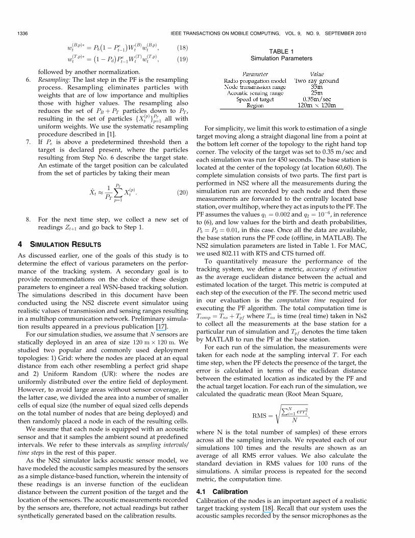
We first evaluate the performance of the PF-based trackingcomparing it with a simple triangulation-based trackingsystem [2] for different number of nodes. For triangulation,we assumed that the distance estimates by measuringpropagation delays are within þ=� 5 percent of the actual

AHMED ET AL.: DETECTION AND TRACKING USING PARTICLE-FILTER-BASED WIRELESS SENSOR NETWORKS 1337

TABLE 2Summary of the Parameters Estimated for Each Sensor

TABLE 3Summary of c Estimated for Each Sensor for Different Distances

values. Simulation results for PF are obtained by using5,000 particles and sampling interval of 1 sec. Fig. 1 showsRMS tracking error in the target’s location (with error barsrepresenting the standard deviations). Note that there areno error bars for grid deployment for triangulation-basedtracking. This is because the triangulation-based trackingalways produces the same magnitude of error for a givengrid topology (nonprobabilistic estimation). We used fivedifferent uniform random topologies and ran the simula-tion 100 times to calculate the standard deviations in theRMS values for both PF and triangulation.

Fig. 1 shows that PF performs better than triangulation-based tracking for both grid and uniform random deploy-ments. There are two main reasons for the poor performanceby triangulation-based tracking. Firstly, the inaccuracies indistance estimates (taken as a random value betweenþ=� 5 percent for this simulation) affect the triangulation-based localization and secondly for sparse topologies, thetriangulation algorithm introduces errors when distanceestimates are reported by less than three motes required fortriangulation. The results show that PF performs muchbetter than triangulation for sparse topologies and thatdifference between the performance of the two decreases forvery dense topologies, e.g., 100 nodes in 120 m� 120 m area.

4.3 Design Parameters

We next evaluate the effect of various design parameters onthe detection accuracy and computation time of the particle-filter-based tracking system.

4.3.1 Effect of the Number of Deployed Sensor Nodes

Figs. 1a and 1b shows that for grid deployment, the RMStracking error drops from about 7.14 meters for 16 nodes to

2.53 meters for 49 nodes. For UR deployment, thecorresponding value decreases from 6.96 to 3.11 meters.Grid deployment shows overall better performance than theUR deployment. Note that tracking performance for URwith 81 nodes is worse than that with 64 nodes. This can beattributed to the random nature of the UR deploymentstrategy. The UR deployment thus performs better or worsethan the grid deployment depending on the node place-ment with respect to the target trajectory.

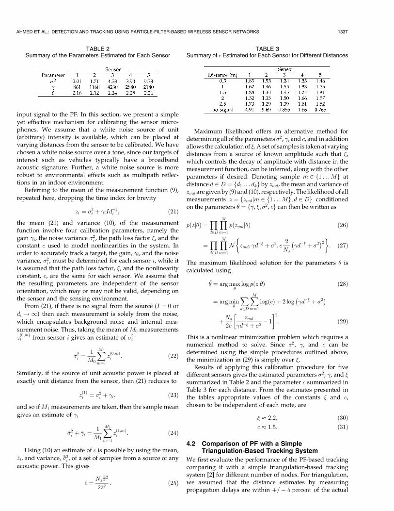
Fig. 2 shows the computation time of the PF versus thenumber of deployed nodes. We can see that the computationtime of the PF grows almost linearly with the number ofdeployed nodes for both grid and uniform random deploy-ment. Packet loss also increases sharply with increase innumber of nodes beyond 49 as shown in Fig. 3. This suggests,that for the given size of the deployment field, target andsensor node characteristics (intensity, sensitivity, etc.), andthe selected networking and simulation parameters, theoptimal density for the deployment of sensor nodes shouldbe somewhere around 34 nodes per 100 m2, which corre-sponds to 49 nodes for the target area under investigation.This node density gives a balance between the error inestimation (RMS tracking error of about 2.5-3 m) and totalcomputation time (about 230 seconds).

4.3.2 Effect of the Number of Generated Particles

Next, we examine the effect of the number of generatedparticles on the performance of the tracking system. Recallthat in our system, a number of particles are randomlygenerated near the sensor nodes. Further, the number ofparticles are independent of the number of deployed nodes(see Section 3) and only the Tpf component of the totalcomputation time varies with change in number of particles.

1338 IEEE TRANSACTIONS ON MOBILE COMPUTING, VOL. 9, NO. 9, SEPTEMBER 2010

Fig. 1. Comparison of PF and triangulation-based tracking.

Fig. 2. Effect of the number of nodes on the computation time. Fig. 3. Effect of the number of nodes on packet loss.

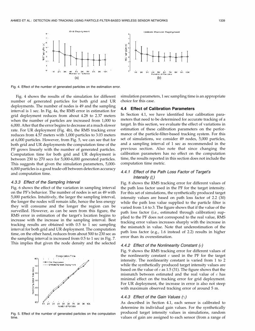
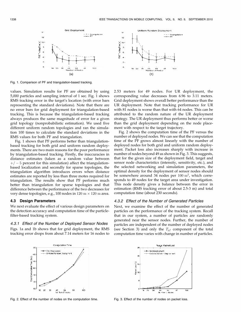
Fig. 4 shows the results of the simulation for differentnumber of generated particles for both grid and URdeployments. The number of nodes is 49 and the samplinginterval is 1 sec. In Fig. 4a, the RMS error in estimation forgrid deployment reduces from about 4.28 to 2.37 meterswhen the number of particles are increased from 1,000 to6,000. After that the error begins to decrease at a much slowerrate. For UR deployment (Fig. 4b), the RMS tracking errorreduces from 4.57 meters with 1,000 particles to 3.03 metersat 6,000 particles. However, from Fig. 5, we can see that forboth grid and UR deployments the computation time of thePF grows linearly with the number of generated particles.Computation time for both grid and UR deployment isbetween 230 to 270 secs for 5,000-6,000 generated particles.This suggests that given the simulation parameters, 5,000-6,000 particles is a good trade-off between detection accuracyand computation time.

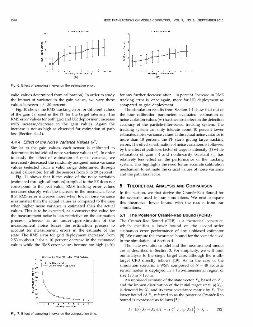
4.3.3 Effect of the Sampling Interval

Fig. 6 shows the effect of the variation in sampling intervalon the PF’s behavior. The number of nodes is set as 49 with5,000 particles. Intuitively, the larger the sampling interval,the longer the nodes will remain idle, hence the less energythey will consume and the longer the region can besurveilled. However, as can be seen from this figure, theRMS error in estimation of the target’s location begins toincrease with the increase in the sampling interval. Besttracking results are obtained with 0.5 to 1 sec samplinginterval for both grid and UR deployment. The computationtime, on the other hand, reduces from about 500 to 230 sec asthe sampling interval is increased from 0.5 to 1 sec in Fig. 7.This implies that given the node density and the selected

simulation parameters, 1 sec sampling time is an appropriatechoice for this case.

4.4 Effect of Calibration Parameters

In Section 4.1, we have identified four calibration para-meters that need to be determined for accurate tracking of atarget. In this section, we evaluate the effect of variations inestimation of these calibration parameters on the perfor-mance of the particle-filter-based tracking system. For thisset of simulations, we consider 49 nodes, 5,000 particles,and a sampling interval of 1 sec as recommended in theprevious section. Also note that since changing thecalibration parameters has no effect on the computationtime, the results reported in this section does not include thecomputation time metric.

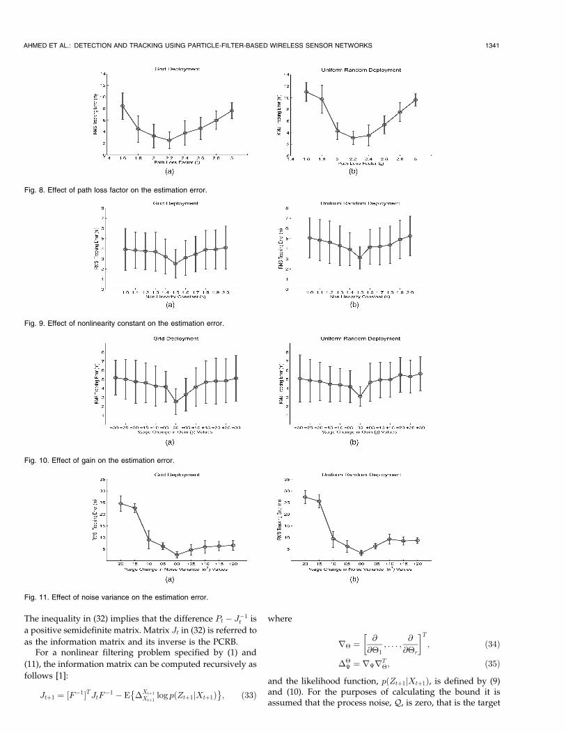
4.4.1 Effect of the Path Loss Factor of Target’s

Intensity (�)

Fig. 8 shows the RMS tracking error for different values ofthe path loss factor used in the PF for the target intensity.For this set of simulations, the synthetically produced targetintensity values are based on path loss factor of 2.2 (30)while the path loss value supplied to the particle filter isvaried from 1.6 to 3. The figure shows that if the value of thepath loss factor (i.e., estimated through calibration) sup-plied to the PF does not correspond to the real value, RMStracking error values increases sharply with the increase inthe mismatch in value. Note that underestimation of thepath loss factor (e.g., 1.6 instead of 2.2) results in highererror than its overestimation.

4.4.2 Effect of the Nonlinearity Constant (c)

Fig. 9 shows the RMS tracking error for different values ofthe nonlinearity constant c used in the PF for the targetintensity. The nonlinearity constant is varied from 1 to 2while the synthetically produced target intensity values arebased on the value of c as 1.5 (31). The figure shows that themismatch between estimated and the real value of c hasminimal effect on the tracking error for grid deployment.For UR deployment, the increase in error is also not steepwith maximum observed tracking error of around 5 m.

4.4.3 Effect of the Gain Values (�)

As described in Section 4.1, each sensor is calibrated todetermine its individual gain values. For the syntheticallyproduced target intensity values in simulations, randomvalues of gain are assigned to each sensor (from a range of

AHMED ET AL.: DETECTION AND TRACKING USING PARTICLE-FILTER-BASED WIRELESS SENSOR NETWORKS 1339

Fig. 4. Effect of the number of generated particles on the estimation error.

Fig. 5. Effect of the number of generated particles on the computationtime.

valid values determined from calibration). In order to studythe impact of variance in the gain values, we vary thesevalues between þ=�30 percent.

Fig. 10 shows the RMS tracking error for different valuesof the gain (�) used in the PF for the target intensity. TheRMS error values for both grid and UR deployment increasewith increase/decrease in the gain values. Again theincrease is not as high as observed for estimation of pathloss (Section 4.4.1).

4.4.4 Effect of the Noise Variance Values (�2)

Similar to the gain values, each sensor is calibrated todetermine its individual noise variance values (�2). In orderto study the effect of estimation of noise variance, weincreased/decreased the randomly assigned noise variancevalues (selected from a valid range determined throughactual calibration) for all the sensors from 5 to 20 percent.

Fig. 11 shows that if the value of the noise variation(estimated through calibration) supplied to the PF does notcorrespond to the real value, RMS tracking error valuesincreases sharply with the increase in the mismatch. Notethat RMS error increases more when lower noise varianceis estimated than the actual values as compared to the casewhen higher noise variance is estimated than the actualvalues. This is to be expected, as a conservative value forthe measurement noise is less restrictive on the estimationprocess, whereas as an under-approximation of themeasurement noise forces the estimation process toaccount for measurement errors in the estimate of thestate. The RMS error for grid deployment increased from2.53 to about 9 for a 10 percent decrease in the estimatedvalues while the RMS error values become too high ð>20Þ

for any further decrease after �10 percent. Increase in RMS

tracking error is, once again, more for UR deployment as

compared to grid deployment.The simulation results from Section 4.4 show that out of

the four calibration parameters evaluated, estimation of

noise variation values (�2) has the most effect on the detection

accuracy of the particle-filter-based tracking system. The

tracking system can only tolerate about 10 percent lower

estimated noise variance values. If the actual noise variance is

more than 10 percent, the PF starts giving large tracking

errors. The effect of estimation of noise variations is followed

by the effect of path loss factor of target’s intensity (�) while

estimation of gain (�) and nonlinearity constant (c) has

relatively less effect on the performance of the tracking

system. This highlights the need for an accurate calibration

mechanism to estimate the critical values of noise variance

and the path loss factor.

5 THEORETICAL ANALYSIS AND COMPARISON

In this section, we first derive the Cramer-Rao Bound for

the scenario used in our simulations. We next compare

this theoretical lower bound with the results from our

simulations.

5.1 The Posterior Cramer-Rao Bound (PCRB)

The Cramer-Rao Bound (CRB) is a theoretical construct,

which specifies a lower bound on the second-order

estimation error performance of any unbiased estimator

[5]. We compute this theoretical bound for the scenario used

in the simulations of Section 4.The state evolution model and the measurement model

are as described in Section 3. For simplicity, we will limit

our analysis to the single target case, although the multi-

target CRB directly follows [19]. As in the case of the

simulation scenario, a WSN composed of N ¼ 49 acoustic

sensor nodes is deployed in a two-dimensional region of

size 120 m� 120 m.An unbiased estimate of the state vector Xt, based on Z1:t

and the known distribution of the initial target state, pðX0Þ,is denoted by Xt, and its error covariance matrix by Pt. The

lower bound of Pt, referred to as the posterior Cramer-Rao

bound is expressed as follows [5]:

Pt¼: E ðXt �XtÞðXt �XtÞT jz1:t; pðX0Þn o

� J�1t : ð32Þ

1340 IEEE TRANSACTIONS ON MOBILE COMPUTING, VOL. 9, NO. 9, SEPTEMBER 2010

Fig. 6. Effect of sampling interval on the estimation error.

Fig. 7. Effect of sampling interval on the computation time.

The inequality in (32) implies that the difference Pt � J�1t is

a positive semidefinite matrix. Matrix Jt in (32) is referred to

as the information matrix and its inverse is the PCRB.For a nonlinear filtering problem specified by (1) and

(11), the information matrix can be computed recursively as

follows [1]:

Jtþ1 ¼ ½F�1�TJtF�1 � E�

�Xtþ1

Xtþ1log pðZtþ1jXtþ1Þ

; ð33Þ

where

r� ¼@

@�1; . . . ;

@

@�r

� �T; ð34Þ

��� ¼ r�rT

�; ð35Þ

and the likelihood function, pðZtþ1jXtþ1Þ, is defined by (9)and (10). For the purposes of calculating the bound it isassumed that the process noise, Q, is zero, that is the target

AHMED ET AL.: DETECTION AND TRACKING USING PARTICLE-FILTER-BASED WIRELESS SENSOR NETWORKS 1341

Fig. 8. Effect of path loss factor on the estimation error.

Fig. 9. Effect of nonlinearity constant on the estimation error.

Fig. 10. Effect of gain on the estimation error.

Fig. 11. Effect of noise variance on the estimation error.

trajectory is deterministic. For the measurement model

specified in Section 3.2, the expectation in (33) can be

evaluated as

� E�

�Xtþ1

Xtþ1log pðZtþ1jXtþ1Þ

¼XNi¼1

HTtþ1;iR

�1tþ1;iHtþ1;i; ð36Þ

where Ht;i is the Jacobian of hiðXtÞ evaluated at the true

value of Xt

Ht;i ¼

ðxi � xtÞ��iItd���2t;i

0ðyi � ytÞ��iItd���2

t;i

0�id��t;i

266664

377775; ð37Þ

and R�1t;i is given by

R�1t;i ¼

4cþNs

2c��2i þ �iItd

��t;i

�2; ð38Þ

once again evaluated at the true value of Xt. The terms in

(37) and (38) are as defined in Section 3.

5.2 Comparison of PCRB and Simulation Results

For the PCRB calculations, the initial state vector was

chosen as

X0 ¼ ½15 0:25 5 0:25 0:7�T ; ð39Þ

where the first and the third components are in meters, while

the second and the fourth components are in meters/sec. For

the purposes of this work, the initial J0 was approximated as

a diagonal matrix with

J�10 ¼ P0 ¼ diagð½0:1 0:05 0:1 0:05 0:01�2Þ: ð40Þ

The displayed error bounds are computed as follows:

bt ¼ffiffiffiffiffiffiffiffiffiffiffiffiffiffiffiffiffiffiffiffiffiffiffiffiffiffiffiffiffiffiffiffiffiffiffiffiffiffiffiffiJ�1t ½1; 1� þ J�1

t ½3; 3�q

; ð41Þ

where J�1t ½1; 1� and J�1

t ½3; 3� are the diagonal elements of the

inverse of the information matrix corresponding to the x

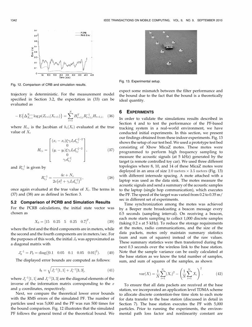
and y coordinates, respectively.Next, we compare the theoretical lower error bounds

with the RMS errors of the simulated PF. The number of

particles used was 5,000 and the PF was run 500 times for

the bound comparison. Fig. 12 illustrates that the simulated

PF follows the general trend of the theoretical bound. We

expect some mismatch between the filter performance andthe bound due to the fact that the bound is a theoreticallyideal quantity.

6 EXPERIMENTS

In order to validate the simulations results described inSection 4 and to test the performance of the PF-basedtracking system in a real-world environment, we haveconducted initial experiments. In this section, we presentour findings obtained from these indoor experiments. Fig. 13shows the setup of our test bed. We used a prototype test bedconsisting of Xbow MicaZ motes. These motes wereprogrammed to perform high frequency sampling tomeasure the acoustic signals (at 5 kHz) generated by thetarget (a remote controlled toy car). We used three differenttopologies where 8, 10, and 14 of these MicaZ motes weredeployed in an area of size 2:0 meters� 3:5 meters (Fig. 13)with different internode spacing. A mote attached with alaptop was used as the data sink. The motes measure theacoustic signals and send a summary of the acoustic samplesto the laptop (single hop communication), which executesthe PF. The speed of the target was varied from 0.2 to 0.35 m/sec in different set of experiments.

Time synchronization among the motes was achievedby a Beeper mote broadcasting a beacon message every0.5 seconds (sampling interval). On receiving a beacon,each mote starts sampling to collect 1,000 discrete samples(taking 0.2 s at 5 kHz). To reduce the storage requirementsat the motes, radio communications, and the size of thedata packets, motes only maintain summary statistics(sum and sum of squares) instead of the raw values.These summary statistics were then transferred during thenext 0.3 seconds over the wireless link to the base station.Note that the sample variance can be easily calculated atthe base station as we know the total number of samples,sum, and sum of squares of the samples, as shown

varðXÞ ¼ 1

N

XNs

i¼1

ðXiÞ2 �1

N

XNs

i¼1

Xi

!2

: ð42Þ

To ensure that all data packets are received at the basestation, we incorporated an application level TDMA schemeto allocate discrete contention-free time slots to each motefor data transfer to the base station (discussed in detail inSection 7). The base station executes the PF with 5,000particles. Prior to running the experiments, the environ-mental path loss factor and nonlinearity constant are

1342 IEEE TRANSACTIONS ON MOBILE COMPUTING, VOL. 9, NO. 9, SEPTEMBER 2010

Fig. 12. Comparison of CRB and simulation results.Fig. 13. Experimental setup.

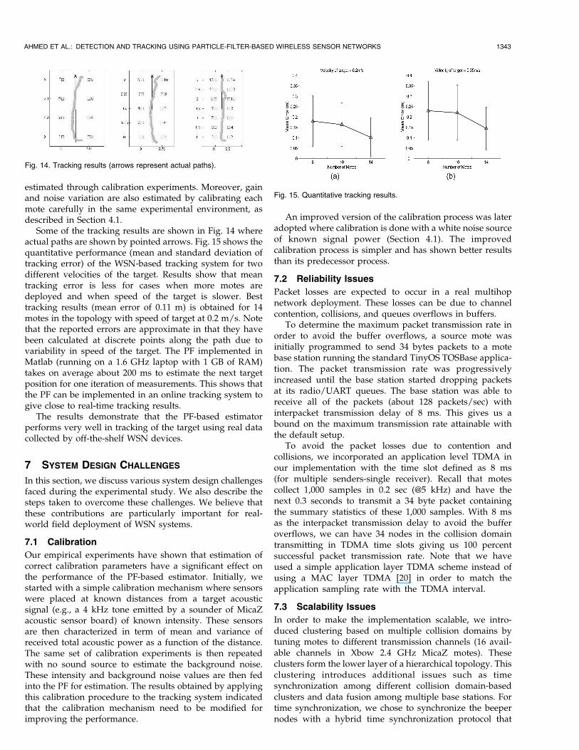
estimated through calibration experiments. Moreover, gainand noise variation are also estimated by calibrating eachmote carefully in the same experimental environment, asdescribed in Section 4.1.

Some of the tracking results are shown in Fig. 14 whereactual paths are shown by pointed arrows. Fig. 15 shows thequantitative performance (mean and standard deviation oftracking error) of the WSN-based tracking system for twodifferent velocities of the target. Results show that meantracking error is less for cases when more motes aredeployed and when speed of the target is slower. Besttracking results (mean error of 0.11 m) is obtained for 14motes in the topology with speed of target at 0.2 m/s. Notethat the reported errors are approximate in that they havebeen calculated at discrete points along the path due tovariability in speed of the target. The PF implemented inMatlab (running on a 1.6 GHz laptop with 1 GB of RAM)takes on average about 200 ms to estimate the next targetposition for one iteration of measurements. This shows thatthe PF can be implemented in an online tracking system togive close to real-time tracking results.

The results demonstrate that the PF-based estimatorperforms very well in tracking of the target using real datacollected by off-the-shelf WSN devices.

7 SYSTEM DESIGN CHALLENGES

In this section, we discuss various system design challengesfaced during the experimental study. We also describe thesteps taken to overcome these challenges. We believe thatthese contributions are particularly important for real-world field deployment of WSN systems.

7.1 Calibration

Our empirical experiments have shown that estimation ofcorrect calibration parameters have a significant effect onthe performance of the PF-based estimator. Initially, westarted with a simple calibration mechanism where sensorswere placed at known distances from a target acousticsignal (e.g., a 4 kHz tone emitted by a sounder of MicaZacoustic sensor board) of known intensity. These sensorsare then characterized in term of mean and variance ofreceived total acoustic power as a function of the distance.The same set of calibration experiments is then repeatedwith no sound source to estimate the background noise.These intensity and background noise values are then fedinto the PF for estimation. The results obtained by applyingthis calibration procedure to the tracking system indicatedthat the calibration mechanism need to be modified forimproving the performance.

An improved version of the calibration process was lateradopted where calibration is done with a white noise sourceof known signal power (Section 4.1). The improvedcalibration process is simpler and has shown better resultsthan its predecessor process.

7.2 Reliability Issues

Packet losses are expected to occur in a real multihopnetwork deployment. These losses can be due to channelcontention, collisions, and queues overflows in buffers.

To determine the maximum packet transmission rate inorder to avoid the buffer overflows, a source mote wasinitially programmed to send 34 bytes packets to a motebase station running the standard TinyOS TOSBase applica-tion. The packet transmission rate was progressivelyincreased until the base station started dropping packetsat its radio/UART queues. The base station was able toreceive all of the packets (about 128 packets/sec) withinterpacket transmission delay of 8 ms. This gives us abound on the maximum transmission rate attainable withthe default setup.

To avoid the packet losses due to contention andcollisions, we incorporated an application level TDMA inour implementation with the time slot defined as 8 ms(for multiple senders-single receiver). Recall that motescollect 1,000 samples in 0.2 sec (@5 kHz) and have thenext 0.3 seconds to transmit a 34 byte packet containingthe summary statistics of these 1,000 samples. With 8 msas the interpacket transmission delay to avoid the bufferoverflows, we can have 34 nodes in the collision domaintransmitting in TDMA time slots giving us 100 percentsuccessful packet transmission rate. Note that we haveused a simple application layer TDMA scheme instead ofusing a MAC layer TDMA [20] in order to match theapplication sampling rate with the TDMA interval.

7.3 Scalability Issues

In order to make the implementation scalable, we intro-duced clustering based on multiple collision domains bytuning motes to different transmission channels (16 avail-able channels in Xbow 2.4 GHz MicaZ motes). Theseclusters form the lower layer of a hierarchical topology. Thisclustering introduces additional issues such as timesynchronization among different collision domain-basedclusters and data fusion among multiple base stations. Fortime synchronization, we chose to synchronize the beepernodes with a hybrid time synchronization protocol that

AHMED ET AL.: DETECTION AND TRACKING USING PARTICLE-FILTER-BASED WIRELESS SENSOR NETWORKS 1343

Fig. 15. Quantitative tracking results.

Fig. 14. Tracking results (arrows represent actual paths).

incorporates accurate byte level time stamping from Flood-ing Time Synchronization Protocol (from Vanderbilt Uni-versity) [21] in simple pairwise message exchanges of theTime synchronization Protocol for Sensor Networks (TPSN)protocol [22]. The time stamps are made at each byteboundary after the SYNC bytes as they are transmitted orreceived to counter the nondeterministic delays in radiomessage delivery in WSN.

We have conducted further experiments with multiplecollision domains with 25 nodes [17] and 36 nodes gridtopologies (not reported in this paper due to spacelimitations). All nodes were able to successfully transmittheir data packets to their respective base stations.

8 CONCLUSION AND FUTURE WORK

In this paper, we have presented a detailed evaluation ofthe performance of a WSN tracking system, which employsthe PF algorithm. We developed a simple yet effectivemechanism for calibrating off-the-shelf sensor motes. Weobserved the effect of various design and calibrationparameters such as number of deployed nodes, number ofgenerated particles, sampling interval, path loss factor,noise variations, gain, and nonlinearity constant on theestimation accuracy and computation time of the trackingsystem. We also made recommendations on the optimalvalues for these parameters, which achieve an acceptabletrade-off between accuracy and complexity. Moreover, weidentified that among the calibration parameters, estimationof the noise variation values has the most significant effecton the performance of the tracking system. It is pertinent tomention here that the characteristics of the target such as itsvolume and speed also effect the choice of these designparameters. These recommendations on the choice ofdesign parameters can be utilized to engineer a real WSN-based tracking solution. We also derived the theoreticallower bound, the CRB, and demonstrated that the resultsfrom our simulations are comparable to the bound.

We discuss the challenges experienced in implementinga prototype of our system using off-the-shelf sensor nodes.We describe custom algorithms that were implemented forsuccessfully realizing the system. We found that ourprototype comprising of off-the-shelf sensor nodes cansuccessfully track the moving target in several scenarios.Our experimental results are quite promising and suggestthat low-cost sensor nodes can effectively complementsophisticated target detection hardware.

In future, we plan to do a real-time implementation ofthe PF-base tracking system and to test the implementationin the outdoor environment.

ACKNOWLEDGMENTS

This paper is a result of collaboration between UNSW(School of Computer Science and Engineering) and DSTO(ISR Division).

REFERENCES

[1] B. Ristic, S. Arulampalam, and N. Gordon, Beyond the KalmanFilter: Particle Filters for Tracking Applications. Artech House, 2004.

[2] Q. Wang, W. Chen, R. Zheng, K. Lee, and L. Sha, “Acoustic TargetTracking Using Tiny Wireless Sensor Devices,” Proc. Second Int’lConf. Information Processing in Sensor Networks (IPSN ’03), pp. 642-657, 2003.

[3] L. Gu, D. Jia, P. Vicaire, T. Yan, L. Luo, A. Tirumala, Q. Cao, T. He,J.A. Stankovic, T. Abdelzaher, and B.H. Krogh, “LightweightDetection and Classification for Wireless Sensor Networks inRealistic Environments,” Proc. ACM SenSys, pp. 205-217, 2005.

[4] M.F. Duarte and Y.H. Hu, “Vehicle Classification in DistributedSensor Networks,” J. Parallel and Distributed Computing, vol. 64,no. 7, pp. 826-838, 2004.

[5] H.L. Van Trees, Detection, Estimation and Modulation Theory (Part I).John Wiley and Sons, 1968.

[6] A. Ledeczi, A. Nadas, P. Volgyesi, G. Balogh, B. Kusy, J. Sallai, G.Pap, S. Dora, K. Molnar, M. Maroti, and G. Simon, “CountersniperSystem for Urban Warfare,” ACM Trans. Sensor Networks, vol. 1,no. 2, pp. 153-177, 2005.

[7] T. He, S. Krishnamurthy, J.A. Stankovic, T.F. Abdelzaher, L. Luo,R. Stoleru, T. Yan, L. Gu, J. Hui, and B. Krogh, “An Energy-Efficient Surveillance System Using Wireless Sensor Networks,”Proc. ACM MobiSys, pp. 270-283, 2004.

[8] M.J. Coates and G. Ing, “Sensor Network Particle Filters: Motes asParticles,” Proc. IEEE Workshop Statistical Signal Processing,pp. 1152-1157, 2005.

[9] C. Taylor, A. Rahimi, J. Bachrach, H. Shrobe, and A. Grue,“Simultaneous Localization, Calibration, and Tracking in an AdHoc Sensor Network,” Proc. Fifth Int’l Conf. Information Processingin Sensor Networks (IPSN ’06), pp. 27-33, 2006.

[10] B. Kusy, J. Sallai, G. Balogh, A. Ledeczi, V. Protopopescu, J.Tolliver, F. DeNap, and M. Parang, “Radio InterferometricTracking of Mobile Wireless Nodes,” Proc. Fifth Int’l Conf. MobileSystems, Applications and Services (MobiSys ’07), pp. 139-151, 2007.

[11] L. Klingbeil and T. Wark, “A Wireless Sensor Network for Real-Time Indoor Localization and Motion Monitoring,” Proc. SeventhInt’l Conf. Information Processing in Sensor Networks (IPSN ’08),pp. 39-50, 2008.

[12] M. Bolic, P.M. Djuri, and S. Hong, “Resampling Algorithms andArchitectures for Distributed Particle Filters,” IEEE Trans. SignalProcessing, vol. 53, no. 7, pp. 2442-2450, July 2005.

[13] R. Brooks, P. Ramanathan, and A. Sayeed, “Distributed TargetClassification and Tracking in Sensor Networks,” Proc. IEEE,vol. 91, no. 8, pp. 1163-1171, Aug. 2003.

[14] D.J. Salmond and H. Birch, “A Particle Filter for Track-Before-Detect,” Proc. Am. Control Conf., 2001.

[15] T. Schon, F. Gustafsson, and P.-J. Nordlund, “MarginalizedParticle Filters for Mixed Linear/Nonlinear State-Space Models,”IEEE Trans. Signal Processing, vol. 53, no. 7, pp. 2279-2289, July2005.

[16] M.G. Rutten, N.J. Gordon, and S. Maskell, “Recursive Track-before-Detect with Target Amplitude Fluctuations,” IEE Proc.Radar Sonar Navigation, vol. 152, no. 5, pp. 345-352, Oct. 2005.

[17] N. Ahmed, M. Rutten, T. Bessell, Y. Dong, S. Kanhere, N. Gordon,and S. Jha, “Performance Evaluation of a Wireless Sensor NetworkBased Tracking System,” Proc. Fifth IEEE Int’l Conf. Mobile Ad Hocand Sensor Systems (MASS ’08), Oct. 2008.

[18] K. Whitehouse and D. Culler, “Calibration as Parameter Estima-tion in Sensor Networks,” Proc. ACM Int’l Workshop Wireless SensorNetworks and Applications (WSNA ’02), pp. 59-67, 2002.

[19] B. Ristic and M. Morelande, “Cramer-Rao Bound for MultipleTarget Tracking Using Intensity Measurements,” Proc. Conf.Information, Decision and Control (IDC ’07), pp. 354-259, Feb. 2007.

[20] K.K. Chintalapudi and L. Venkatraman, “On the Design of MacProtocols for Low-Latency Hard Real-Time Discrete ControlApplications over 802.15.4 Hardware,” Proc. Int’l Conf. InformationProcessing in Sensor Networks (IPSN ’08), pp. 356-367, Apr. 2008.

[21] M. Maroti, B. Kusy, G. Simon, and A. Ledeczi, “The FloodingTime Synchronization Protocol,” Proc. Second ACM Conf. EmbeddedNetworked Sensor Systems (SenSys ’04), pp. 39-49, Nov. 2004.

[22] S. Ganeriwal, R. Kumar, and M.B. Srivastava, “Timing-SyncProtocol for Sensor Networks,” Proc. First ACM Conf. EmbeddedNetworked Sensor Systems (SenSys ’03), pp. 138-149, Nov. 2003.

1344 IEEE TRANSACTIONS ON MOBILE COMPUTING, VOL. 9, NO. 9, SEPTEMBER 2010

Nadeem Ahmed received the BE degree fromthe University of Engineering and Technology,Lahore, Pakistan, and the MS and PhD degreesin computer sciences from the University of NewSouth Wales (UNSW), Sydney, Australia, in2000 and 2007, respectively. He is currently aresearch associate with the School of ComputerScience and Engineering at UNSW. His re-search interests include wireless sensor net-works and mobile ad hoc networks. He is a

member of the IEEE.

Mark Rutten received the BSc degree incomputer science and theoretical physics in1994, the BE degree in electrical engineeringin 1995, and the MSc degree in signal andinformation processing in 1998, all from TheUniversity of Adelaide, and the PhD degree inelectrical and electronic engineering from theUniversity of Melbourne in 2005. Since 1996, hehas been working with the Defence Science andTechnology Organization in Edinburgh, Austra-

lia, working with the Tracking and Sensor Fusion group from 1999. Hisresearch interests include nonlinear filtering, tracking, and track fusion.

Travis Bessell received the BE degree incomputer systems engineering from FlindersUniversity in 2005 and the MSc degree in signaland information processing from The Universityof Adelaide in 2008. Since 2005, he has beenworking with the Defence Science and Technol-ogy Organization, Edinburgh, Australia, workingwith the Tracking and Sensor Fusion group. Hisresearch interests include wireless sensor net-works, nonlinear filtering, and tracking.

Salil S. Kanhere received the BE degree inelectrical engineering from the University ofBombay, India, in 1998, and the MS and PhDdegrees in electrical engineering from DrexelUniversity, Philadelphia, in 2001 and 2003,respectively. He is currently a senior lecturerwith the School of Computer Science andEngineering at the University of New SouthWales, Sydney, Australia. His current researchinterests include wireless sensor networks,

vehicular communication, mobile computing, and network security. Heis a member of the IEEE and the ACM.

Neil Gordon received the BSc degree inmathematics and physics from NottinghamUniversity, United Kingdom, in 1988, and thePhD degree in statistics from Imperial College,University of London, in 1993. From 1988 to2002, he was with various research groupswithin DERA and QinetiQ working in the areas ofmissile guidance, target tracking, and statisticaldata processing. Since August 2002, he hasbeen with DSTO in Australia where he is

currently the head of the Tracking and Sensor Fusion research group.He is a coeditor/coauthor of two books on particle filtering. He is amember of the IEEE.

Sanjay Jha received the PhD degree from theUniversity of Technology, Sydney, Australia. Heis a professor and head of the Network Group inthe School of Computer Science and Engineer-ing at the University of New South Wales. Hisresearch activities cover a wide range of topicsin networking including wireless sensor net-works, ad hoc/community wireless networks,resilience/quality of service (QoS) in IP net-works, and active/programmable network. He

has published more than 100 articles in high quality journals andconferences. He is the principal author of the book Engineering InternetQoS and a coeditor of the book Wireless Sensor Networks: A SystemsPerspective. He is an associate editor of the IEEE Transactions onMobile Computing. He was a member-at-large for the TechnicalCommittee on Computer Communications (TCCC) of the IEEEComputer Society for a number of years. He has served on programcommittees of several conferences. He was the technical programcommittee chair of the IEEE Local Computer Networks LCN2004 andATNAC04 conferences, and the cochair or general chair of the Emnets-1and Emnets-II workshops, respectively. He was also the general chair ofthe ACM SenSys 2007 symposium. He is a senior member of the IEEEand the IEEE Computer Society.

. For more information on this or any other computing topic,please visit our Digital Library at www.computer.org/publications/dlib.

AHMED ET AL.: DETECTION AND TRACKING USING PARTICLE-FILTER-BASED WIRELESS SENSOR NETWORKS 1345