DETECTING THE BREAKDOWN OF TRAFFIC

1

DETECTING THE BREAKDOWN OF TRAFFIC

Submission Date: July 12, 2002

Word count: 6537 words.

Xi Zou and David Levinson

Department of Civil Engineering, University of Minnesota

500 Pillsbury Dr. SE, Minneapolis, MN 55455

Phone: 612-625-4021, [email protected];

Phone: 612-625-6354, Fax: 612-626-7750, [email protected]

Zou, Xi and David Levinson (2003), Detecting the Breakdown of Traffic. Presented at Transportation Research Board Conference, January 12 –– 16 2003 Washington DC (Session 732) (03-2153)

2

ABSTRACT

Timely traffic prediction is important in advanced traffic management systems to make

possible rapid and effective response by traffic control facilities. From the observations

of traffic flow, the time series present repetitive or regular behavior over time that

distinguishes time series analysis of traffic flow from classical statistics, which assumes

independence over time. By taking advantage of tools in frequency domain analysis, this

paper proposes a new criterion function that can detect the onset of congestion. It is found

that the changing rate of the cross-correlation between density dynamics and flow rate

determines traffic transferring from free flow phase to the congestion phase. A definition

of traffic stability is proposed based on the criterion function. The new method suggests

that an unreturnable transition will occur only if the changing rate of the cross-correlation

exceeds a threshold. Based on real traffic data, detection of congestion is conducted in

which the new scheme performs well compared to previous studies.

Keyword: Traffic Breakdown, Congestion Detection, Density Dynamics, Traffic

Stability


3

1. INTRODUCTION

Reports of travel time and route guidance aim to assist drivers and traffic managers. Successful

traffic control systems are based on the quantity and accuracy of the data obtained from the road

network. All of these kinds of information must be estimated or predicted from current and

historical traffic detector data. Many schemes have been used to make reliable traffic flow

predictions, such as dynamic linear models (1), nonparametric regression (2), neural networks (3;

4), ARIMAX (5) and Kalman filtering (6). All of these efforts are mainly based on the previous

time-series information from a single location.

Traffic transition is such a complex phenomenon that no single theory, such as car-

following model (7), queuing theory (8), kinetic theory (9), cellular automata (10), higher-order

models (11) and kinetic wave theory (12), completely describe it. The cause of phase transitions

or the physical explanation of the critical phenomenon in traffic flow is still an unresolved

problem. The onset of phase transition is worth investigating because it sheds light on prediction

or detection of traffic breakdown. That is, if one can understand the generation of phase

transition from free flow to jam phases, a potential traffic breakdown can be detected.

Furthermore, if one can find the causes that generate the phase transition and can detect these

causes, control could be implemented earlier to alleviate or eliminate the potential congestion.

Kerner (13; 14; 15) proposed the existence of three distinct phases of traffic: Free flow in which

flow is a linear function of density; stop-and-go states (wide-moving jams); and “synchronized

flow” which is between free flow and stop-and-go states. In synchronized flow, traffic is moving

at lower density; and it appears as a cluster underneath the free-flow line on the q-k curve. His

theory was further developed (16, 17) which yielded an approach to predict traffic transitions

(19). Daganzo et al. (20) argued that the spontaneous nature of queue generation in the Kerner’s


4

theory could be deterministically explained by a Markovian model, in which the results of

“disturbances” are determined by the initial state of the traffic. But they accepted the

incompleteness of this theory and expected an explanation of “the genesis of the disturbances or

the rate at which they grow.” Further empirical observation and simulation studies of Treiber et

al. (21) and Lee et al. (22) showed that there is state and phase “structure” in the traffic flow

patterns where the relation among density, speed and flow rate are changed, i.e., from one phase

to another. Nagatani, T. (23) provided a theoretical explanation of the phase transition and

critical phenomenon occurring in traffic based on thermodynamic theory and a car-following

model and derived a stability condition for uniform flow. He showed that the jamming transition

could be explained by the phase transitions and critical phenomena.

On the other hand, traffic transitions are closely related to the stability issues of traffic

flow. At a macroscopic scale, traffic flow is the aggregation of strings and single vehicles in

many sections of motorway. Traffic flow stability deals with the evolution of aggregate velocity

and density in response to change in the flow rate. Darbha and Rajagopal (24) proposed that,

“Traffic flow stability can be guaranteed only if the velocity and density solutions of the coupled

set of equations is stable, i.e., only if stability with respect to automatic vehicle following and

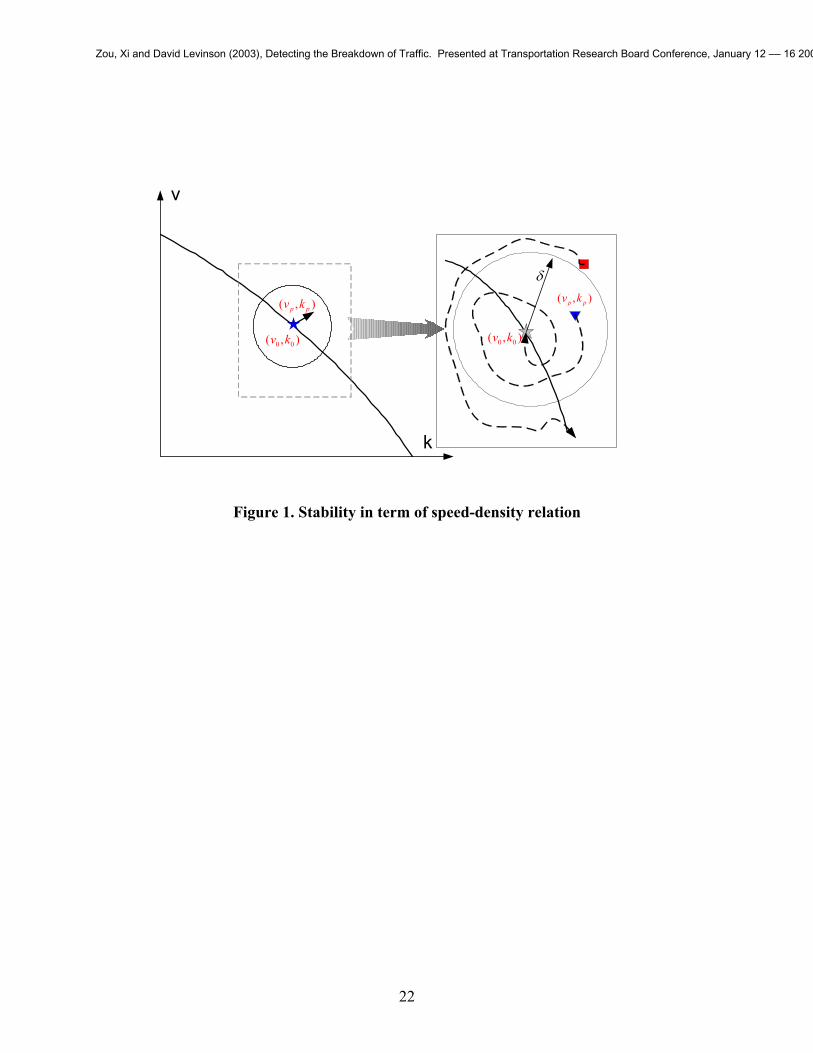
stability with respect to density evolution is guaranteed.” Their definition of Traffic Flow

Stability for automated vehicle traffic is in the sense of Lyapunov and can be described in Figure

1. ),( 00 kv is a steady state of traffic. Here the traffic flow is defined to be stable when the

disturbance ),( pp kv does not exceed a boundary if its initial value is within a limit, and, in the

end, the disturbance becomes zero. As shown in the enlarged figure in Figure 1, if the initial state

is within the boundary (the triangle point), it goes to the equilibrium point ),( 00 kv in the end; but

if the initial state is beyond the boundary (the rectangle point), it does not converge to the


5

equilibrium point but goes to other indefinite states. This definition is very strong in that the

disturbance must be eliminated over time by its own movement. In real-world traffic,

disturbances or unstable traffic usually are eliminated because of light demand inflows which

happen from time to time. On the other hand, it’s also a loose definition because it doesn’t

present the traffic state change from free flow to congestion in which the change of the “nominal

state of traffic” itself is the source of traffic flow instability. Thus, a Lyapunov stability

definition in terms of speed-density relation may not work well in describing traffic stability. In

this paper, a definition of traffic flow stability will be proposed based on a new criterion

function.

This paper aims to detect the transition earlier comparing to the previous studies. Instead

of using time domain analysis methods, this paper applies frequency domain tools in traffic flow

studies. Stathopoulos and Karlaftis (26) first studied this topic and suggested the development of

multivariate state-space models for short-term flow forecasting. It is well known that the

frequency domain analysis quantitatively describes the oscillations of movements. In addition, it

is a straightforward idea that the oscillation of traffic flow could be used as the representative of

stability and/or robustness. Ioerger et al. (26) also proposed applications of signal detection tools

to identify traffic congestion. In their work, they added some new properties of synchronized

flow, wherein flow becomes less a function of density, but more dependent on its recent history.

They proposed a method to detect the generation of synchronized flow. Its advantages and

disadvantages will be illustrated and compared with the new method in the sections below.

In section 2, some tools that might be used in traffic studies will be discussed. A new

criterion function and its implementation method will be proposed. An application of the newly

proposed criterion function in traffic flow stability is also presented in Section 2. Section 3


6

describes the real-world traffic data that are investigated in this paper and shows performances of

studied detection methods in identifying real-world traffic congestions. Section 4 concludes

based on the former results and proposes further research.

2. METHODOLOGY

2.1 Detection Criterion

Signal processing theories provide numerous methods to process blurred signals and data from

natural and man-made systems. From the traffic engineer’s point of view, one can find their

applications to detect many implicit characteristics that hide in the great amount of traffic data.

In the time domain, signals are shown as the summation of all frequency components. In the

frequency domain, the level of each signal can be displayed separately. Traffic data, such as

volume and occupancy information obtained from detectors on the road, are always treated as

time series. Normally, there are two approaches to characterizing the variance in time series: (1)

To describe the variance in the product of measurements separated in space or time. This results

in auto-covariance or autocorrelation functions for the time series. (2) To describe the variance in

the tendency of measurements in the space or time. This results in a cross-correlation function

for the time series. On the other hand, our aim is to develop methods that can be put into real-

world use. We require they (1) only use historical and current data; (2) can be implemented in

real-time computation; (3) must be discrete in term of time separation.

Filters are the most direct application of signal processing theory after we obtain the

decomposed signal in frequency domain. Convolution computations are used in filters because

they can eliminate specified frequency components outside the given frequency window.

∫∞

∞−−= dutuhtfhfC )()(),( (1)


7

where: ( , )C f h is the convolution of function ( )f t and ( )h t ; t and u are time variables. A low

pass filter deletes high frequency components to present the basic movement of the signal. But

high frequency components, which represent noise and oscillations in the movement, are also

important. In traffic engineering, oscillations in speed and flow rate should be treated as normal

except those that cause traffic breakdown.

Based on microscopic observations, Ioerger et al.’s (26) method suggests, “Drivers might

decrease their velocities in anticipation of increased density in front of them.” So they expected

an observation of speed drop that depends on the derivative of the density (6). Template

Convolution is used to detect pulses in density derivatives. To achieve this, they used a sine

curve to approximate a large pulse in the density gradient and come up with a “Detector”

( )tσ as:

{ }2( ) ( ,sin( ;0.. )) ( , sin( ;0..2 ))

( )

t C g u C g udg k udt

σ π π = − −

=

(2)

where: g is the derivative of density; t and u are time variables. Though their detection method

can pick up speed drops in traffic, it still has some disadvantages. It only considers the density

gradient; it over-simplifies pulse formation; and it lacks a physical illustration of its source.

Other disadvantages in performance will be shown in the sections below.

In this paper, we will take advantage of both low-pass and high-pass filters to pick up

dynamics in traffic flow. The idea is first to find out the moving-average of a signal (density in

this case):

><<<

=

=

12

12

,01

)(

))(),((

ttttttt

tP

tPtkCklow

(3)


8

The filtered high frequency components *( )k t are restored by subtracting low frequency

components from the original signal, which is defined as Density Dynamics:

)()()(* tktktk low−= (4)

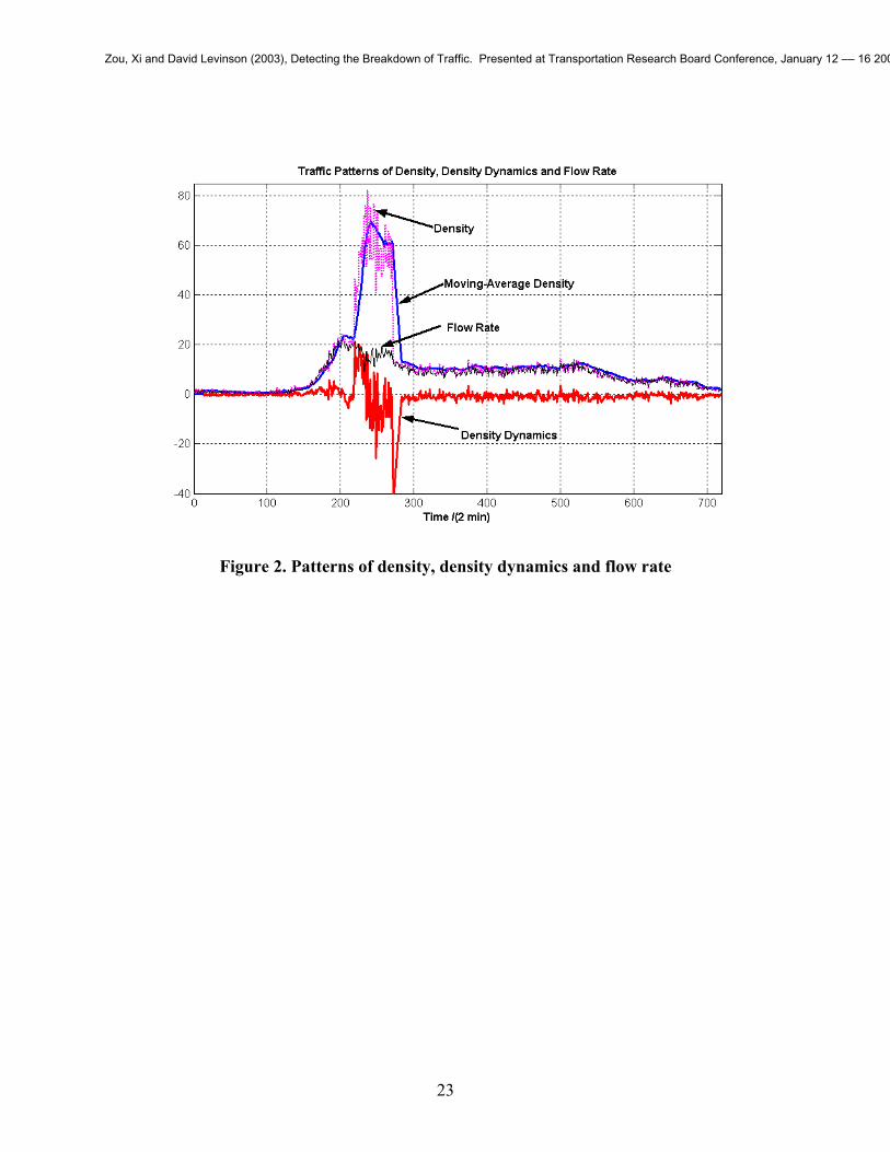
An example of patterns of flow rate, density and density dynamics in a weekday is shown

in Figure 2. Density Dynamics *( )k t is used to present the temporary changes of k above the

average. As we discussed above, *( )k t is summation of the high frequency components of k.

The relation between *( )k t and q(t) is important in that it provides information on the critical

change occurring in traffic flow.

Cross-Correlation is always used to detect the diversity of measurements:

∫∞

∞−+= dutuhtfhf )()(, (5)

where: ,f h is the cross-correlation of function ( )f t and ( )h t ; t and u are time variables. In this

research, template cross-correlation is used to detect the variation in the relation of two quantities

along time, for instance:

qkqkcorr ⋅= ** max),( (6)

where *k and q are templates of *k and q, respectively, move simultaneously. Template means

a consecutive portion of data in a series.

From the observation of the traffic flow, such as patterns in Figure 2, one can see that

flow rate q (volume), density k (occupancy), and speed v have different patterns before and

within congestion. Density and flow rate have similar patterns except under congested

conditions. In congestion, the flow rate q increases a little bit and then drops. The density k

increases sharply compared to the flow rate, and thus the speed v drops correspondingly


9

according to q k v= ⋅ relation. Loop detectors provide accurate flow rate and an estimate of

density. Because the lack of the information on average vehicle length, the density estimate is

not accurate, nor is the estimated speed. Instead of using these rough values, one can see their

changes with time indicators of traffic quality.

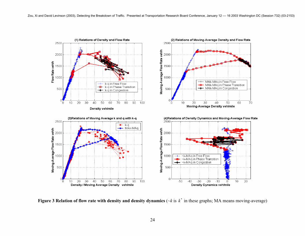
In this paper, we propose a new detection method to detect potential traffic congestion.

Figure 3, obtained from real traffic data, presents the relations among density, density dynamics

and flow rate. It includes two-minute traffic data from a detector station in a normal weekday.

Figure 3(1) shows a normal k-q relation which could happen in every section of highway

experiencing congestions. It is obviously difficult to find out valuable information from such a

disorderly graph. Figure 3(2) shows the relation between the moving-average k and q. One can

see that an explicit movement of traffic flow in the {k, q} space. Two clusters of traffic states are

distinctly shown in the graph: one is along the free-flow curve; the other is located in the

congestion area. Though this result provides support to our methodology, it is insufficient

because the moving-average computation eliminates most of information about temporary traffic

movement. So we combine the former two graphs in Figure 3(3). As one can see, nearly all of

dynamic traffic movements cluster below the moving-average curve. On the other hand, these

dynamic traffic movements largely go along the moving-average curve in the transition states.

Density dynamics is used to present the difference between the dynamic traffic movement and

the moving-average states, as shown in Figure 3(4). In distilling *k from k, high frequency

components, which represent oscillations of k, are obtained. Meanwhile, the density gradient

information sought by Ioerger’s method is also included.

From Figure 3(4), we can see that the relation between density dynamics and flow rate

only oscillates slightly in the free flow but changes obviously when traffic goes from free flow to


10

congestion. Furthermore, these changes are extraordinarily large in the onset of the phase

transitions. For instance, *k increases greatly in the phase transition from free flow to congestion

and decreases steeply in the transition from congestion to free flow. Our aim is to find a quantity

to describe the variation among these changes. We conduct a template cross-correlation

calculation:

**( , ) maxcorr k q k q= < ⋅ >r r (7)

where *kr and qr are templates of *k and q, respectively, move simultaneously. The template

calculation only uses data in the past and finds the maximum correlation in each step. Cross-

correlation finds the correlation of density dynamics with flow rate. So flow rate is considered in

this scheme, instead of ignoring it as in Ioerger’s method. This improvement is important

because it relates the result to empirical observations. We expect drivers decelerate in response

to many causes ahead, including incidents, lane changing, changing of physical roadway or

traffic queue. These responses result in temporary density disturbances in traffic flow. This

disturbance may cause traffic breakdown, but is not a sufficient condition. Another condition is

the traffic demand exceeds capacity. Traffic flow near the capacity is less stable and will

breakdown under small disturbances. Traffic flow far below the capacity still can breakdown

under very large disturbance such as serious incident or large on-ramp flow. So it is reasonable

to use their cross-correlation instead of a single variable to describe the transition movement.

Furthermore, to detect the onset of the transition, we calculate the derivative of cross-

correlation series:

( )*( ) ( , )dz t corr k qdt

= (8)


11

which generate a new “Detector” function of the traffic patterns. Theoretically, this criterion

function tracks the changing rate of the cross-correlation and yields a pulse that is a timely

advance to the cross-correlation function. The time advance property will be beneficial to

advanced traffic control operation. The performance of this detection method will be present in

the section below.

2.2 Traffic Flow Stability

The computation results based on real world traffic data justified the effectiveness of this

function. It’s shown that there is a traffic breakdown only when 0* )),(()( zqkcorr

dtdtz >= ,

where 0z could be a threshold obtained from experience. If the changing rate of the cross-

correlation exceeds the threshold, the transition is unreturnable. Another important property is

that the criterion function has a singular peak in the onset of the phase transition. These results

indicate that the criterion function might be a mathematical description of transition in traffic

flow which presents the traffic flow moving from stable to instable states.

In deriving the criterion function, we find concentrations of traffic states in both free flow

and congested traffic by means of a moving–average computation, as shown in Figure 3(2). This

intuitively provides support of previous studies that suggest distinct phases in traffic flow. Also,

the transitions that happened between relatively stable phases represent cases when the system

loses or regains stability. Thus the transient condition of traffic flow we obtained sheds light on

the conceptions of traffic stability and robustness.

If the traffic transferring from free flow to congestion that is considered as an unstable

state, we can provide stability criterion as:


12

Stability Criterion:

The traffic flow will remain stable if the changing rate of the cross-correlation between

flow rate and density dynamics is always within a boundary, i.e., 0* )),(()( zqkcorr

dtdtz <= .

Figure 4 illustrates the basic movement of traffic flow in losing and regaining stability.

Our study shows that: if the initial state is within the boundary of stable states cluster, and if the

state transition satisfies the stability criterion, the traffic will remain stable. Otherwise, traffic

will lose stability and become congested. The boundary can be got in real-world experience. This

is a kind of Lyapunov stability. By Lyapunov stability, we mean that state disturbances that

satisfy the boundary conditions remain bounded. Unlike Darbha and Rajagopal’s (24) definition,

the stable states in the {k, q} space is not a single point but a cluster with boundary, which

represents the states of traffic flow more realistically. The new stability criterion directly

provides the explicit condition of traffic transitions in the {k, q} space, rather than the implicit

relation in previous studies. These advantages make this method more practical.

3. ANALYSIS OF REAL TRAFFIC DATA

The data used in this study is from loop detector data on the main interstate freeway near

Minneapolis (27). Minnesota Department of Transportation records a great amount of detector

data, with the flow rate and occupancy on each detector every 30 seconds. Speed can also be

estimated based on a preset average vehicle length.

To simplify the analysis, stations where there is no on and off ramp between them are

chosen for investigation. The data of detector station #579 and # 580 are available for analysis,

which are located on southbound I-35W near the Stinson Boulevard and around 700 meters away

from each other. To simplify the problem, the volumes of three detectors in each station are


13

added together, and the occupancies are averaged. In Mn/DOT, a simplified method to get

estimated speed is used:

speed[i]=5*vol[i]/occ[i] (9)

where: vol[i] is the volume in veh/s; occ[i] is the occupancy; constant 5 feet is a quantity related

to the average length of vehicle. But in the reality, this simplification will result in errors in

speed estimation because the average vehicle length varies greatly over time. For instance, at

night, the proportion of trucks is larger than during daytime. That results in a higher average

length. So in this study, the estimated speed is used only to present the trend of speed movement.

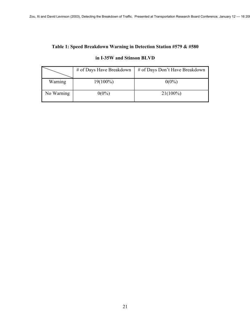
To present the normal pattern of weekday traffic, data from 20 Thursdays from July 6 to

November 16, 2000 in Detection Station #579 and #580 in I-35W and Stinson Blvd. are selected

from the database. Station #579 is an active bottleneck. Station #580 is in the upstream and is

affected by #579. Among these days, no congestion happened on 9 days, morning peak hour

congestion happened on 10 days, afternoon peak hour congestion happened on 2 days. The tests

of the proposed detector are summarized in Table 1, in which the accuracy of the prediction is

satisfactory.

Ioerger’s detector and the new detector are implemented and compared by using real traffic data

from detector stations. Results are presented below. To present the result clearly, scales of some

quantities are changed correspondingly.

3.1 Morning Peak Hour Breakdown

Figure 5 presents the responses of two traffic detectors and the corresponding speed estimate in a

duration including morning peak hour traffic. As one can see, there is a speed breakdown in the

morning peak hour. Both detectors can find the potential changes in traffic. The new detector has


14

a little higher variance in free flow though it doesn’t do harm to the detection. On the other hand,

Ioerger’s detector generates more null peaks that mean nothing about detection. The new

detector has only one main peak. Furthermore, the new detector generates a response 2-3 time

steps ahead of Ioerger’s detector, which means an “early” detection of 4 to 6 minutes ahead.

It is also can be seen in Figure 3 that the up-edge of the main peak appears when the

speed begins to drop. In this case, the value of detector reaches a high level when the speed drops

to 75% of average. An explicit breakdown warning can be generated. If one just uses the speed

estimation as an indicator, no accurate prediction of the speed breakdown can be made at this

point because speed drops to this extent happen so frequently, especially in the early morning or

sometimes in daytime, as shown in Figure 5. On the other hand, there is time duration from the

proposed breakdown warning to the maximum speed drop point. It ranges from 4 minutes to 10

minutes from observations. This time-advance pulse is important because an early detection or

prediction might help generate better traffic control to eliminate or mitigate congestion.

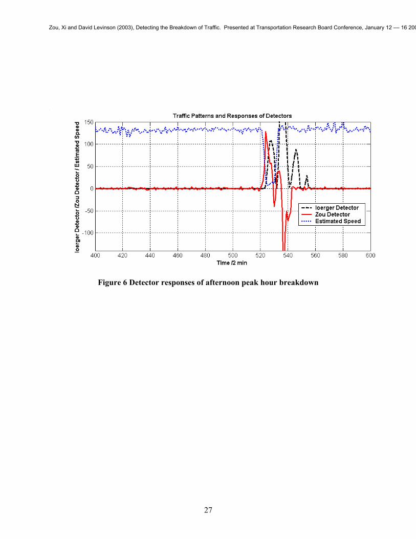
3.2 Afternoon Peak Hour Breakdown

In Figure 6, detection of an afternoon peak hour jam is present. The same situations happen here

and the new detector still performs well. These results show that the proposed detection method

can’t be affected by the daily variation of density and flow rate data and is capable of detecting

congestions occurring in anytime. It should be mentioned here that Ioerger’s detector always

reaches its first peak near the lowest speed. So it is more suitable to detect the extent of

congestion than detecting the onset of phase transition.


15

3.3 No Congestion And Small Speed Drop

Several special traffic patterns are selected to test the reliability of the detector, as shown in

Figure 7. In the case of non-congestion pattern in Figure 7(a), though there is high oscillation of

speed in the early morning, neither of two detectors generates a wrong response. This is

important in that they eliminate errors that always happen if only speed is considered in

breakdown detection.

In the case of slight congestion in Figure 7(b), both detectors perform well by providing

distinct pulse against normal traffic. It should be mentioned that estimated speed drops with

similar amplitude are ignored correctly.

Figure 7(c) shows a wide jam happened in the morning and a slight speed drop in the

afternoon. It is obvious that both detectors can avoid fault detection in speed drop. This property

is important because it means the detector can distinguish the real potential of congestion with

traffic experiencing disturbance.

4. CONCLUSIONS

Based on the former studies that take advantage of traffic information such as density gradient to

identify patterns of traffic congestions, this paper proposed a new criterion function that can

detect traffic breakdown more effectively. Density dynamics and its correlation with flow rate

change clearly when traffic transitions from free flow phase to the congestion phase. The results

of the new method based on real traffic data suggests that (1) there is a traffic breakdown only

when ( )*0( ) ( , )dz t corr k q z

dt= > , where 0z could be a threshold obtained from experience; (2) if

the changing rate of the cross-correlation exceeds the threshold, the transition is unreturnable; (3)

the criterion function has a singular peak in the onset of the phase transition. These conclusions


16

indicate that the criterion function might be a mathematical description of phase transition in

traffic flow.

In deriving the criterion function, we find concentrations of traffic states in both free flow

and congested traffic by means of moving–average computation. This intuitively provides

support of previous studies that suggest distinct phases in traffic flow. Also, the transitions

happened between relatively stable phases represent cases when the system loses or regains

stability. Thus the transient condition of traffic flow we obtained sheds light on the conceptions

of traffic stability and robustness.

Further research on this topic may reveal basic characteristics of traffic congestion. We

seek a physical definition of the stability boundary and studying the singularity of criterion

function. Though some other candidates are studied and considered less effective, the optimality

of the proposed criterion function can’t be guaranteed.


17

REFERENCES

1. Lan, C.J. and Miaou, S.P. (1999). Real-time prediction of traffic flows using dynamic

generalized linear models. Transportation Research Record, 1678, 168-177.

2. Davis, G.A. and Nihan, N.L. (1991). Nonparametric regression and short-term freeway

traffic forecasting. ASCE Journal of Transportation Engineering, Vol. 177, No. 2, 178-188.

3. Nakatsuji, T., Tanaka, M., Nasser, P., Hagiwara, T. (1998). Description of macroscopic

relationships among traffic flow variables using neural network models, Transportation

Research Record, 1510, 11-18.

4. Park, D., Rilett, L.R., Han, G. (1999). Spectral basis neural networks for real-time travel time

forecasting. ASCE Journal of Transportation Engineering, Vol. 125, No. 6, 515-523.

5. Lee, S. and Fambro, D.B. (1999). Application of subset autoregressive integrated moving

average model for short-term freeway traffic volume forecasting. Transportation Research

Record, 1678, 179-188.

6. Okutani, I. and Stephanides, Y.J. (1984). Dynamic prediction of traffic volume through

Kalman filtering theory, Transportation Research part B, Vol. 18B, No. 1, 1-11.

7. Rothery, R. W. (2000). Car following models. In Gartner, N.H., Messer, C., and Rathi, A.K.,

editors, Traffic flow theory, chapter 4. http://www.tfhrc.gov/its/tft/tft.htm, accessed Feb. 2,

2002.

8. Newell, G.G. (1982). Application of queuing theory, Chapman and Hall, 2nd edition.

9. Prigogine, I. And Herman, R. (1971). Kenitic theory of vehicle traffic. NewYork: American

Elsevier.


18

10. Nagel, K. Shreckenberg, M. (1992). A cellular automaton model for freeway traffic. Journal

of Physics I, France, 2: 2221-2229, 1992.

11. Kuhne R. and Michalopoulos, P. (2001) Contimuum flow models. In Gartner, N.H., Messer,

C., and Rathi, A.K., editors, Traffic flow theory, chapter 5.

http://www.tfhrc.gov/its/tft/tft.htm, accessed Feb. 2, 2002.

12. Lighthill, M.J. and Whitham, G.B. (1955). On kinematic wave II: A theory of traffic flow on

long crowded roads. Proceedings of the Royal Society of London, A229: 317-345.

13. Kerner, B.S. (1996b) Experimental properties of complexity in traffic flows, Physical

Review E, Vol. 53, No. 5, May.

14. Kerner, B.S. (1997). Experimental properties of phase trasitions in traffic flow, Physical

Review Letters, Vol. 79 No. 20, Nov. 17.

15. Kerner, B.S. (1998a). Experimental Features of Self-Organization in Traffic Flow, Physical

Review Letters, Vol. 81 No. 17: 3797-3800, Oct. 26.

16. Kerner, B.S. and Rehborn, H. (1998b). German patent publication DE 198 35 979 (day of

notification: August 8th, 1998).

17. Kerner, B.S. Aleksic, M., Denneler, U. (2000). German patent publication DE 199 44 077;

Kerner, B.S. Aleksic, Rehborn, H., Haug, A., Proceedings of 7th ITS world congress on

Intelligent Transport System, Turin, paper No. 2035, 2000.

18. Kerner, B.S. (1996a) Experimental features and characteristics of traffic jams, Physical

Review E, Vol. 53, No. 2: 1297-1300, February.

19. Kerner, B.S. (2001). Tracing and Forecasting of Congested Patterns for Highway Traffic

Management, IEEE ITS Conference Proceedings, Aug.


19

20. Daganzo, C.F., Cassidy, M.J., Bertini, R.L. (1999), Possible explanations of phase transitions

in highway traffic, Transportation Research Part A: 33, 365-379.

21. Treiber, M., Hennecke, A., Helbing, D. (2000). Congested traffic states in empirical

observations and microscopic simulations, Phy. Rev. E, Vol. 62, No. 2, August.

22. Lee, H.Y. et al. (2000), Pahse diagram of congested traffic flow: An empirical study,

Physical Review E, Vol. 62, No. 4, October.

23. Nagatani, T. (1998). Thermofynamic theory for the jamming transition in traffic flow,

Physical Review E, Vol. 58, No.4, October.

24. Darbha, S. and Rajagopal, K. R., (1999). Intelligent cruise control systems and traffic flow

stability, Transportation Research Part C: Emerging Technologies, Volume 7, Issue 6,

December 1999, Pages 329-352.

25. Stathopoulos, A. and Karlaftis, M.G. (2001), Spectral and Cross-Spectral Analysis of Urban

Traffic Flows, 2001 IEEE Intelligent Transportation Systems Conference Proceedings,

August.

26. Ioerger, T.R., Meeks, J.H., Nelson, P., (2001) Investigation of Denity and Fow Relationships

in Congested Traffic Using Videogrametric Data. Proceedings of the 80th Annual Meeting of

the Transportation Research Board, CD-ROM.

27. MnDOT (2001). ftp://vlsi.d.umn.edu/pub/tmcdata, accessed Feb. 2, 2002..


20

List of tables and figures:

Table 1: Speed Breakdown Warning in Detection Station #579 & #580 in I-35W and

Stinson BLVD

Figure 1. Stability in term of speed-density relation

Figure 2. Patterns of density, density dynamics and flow rate

Figure 3 Relation of flow rate with density and density dynamics

Figure 4. Stability change of traffic flow

Figure 5 Detector responses of morning peak hour breakdown

Figure 6 Detector responses of afternoon peak hour breakdown

Figure 7 Detector responses in different situations


21

Table 1: Speed Breakdown Warning in Detection Station #579 & #580

in I-35W and Stinson BLVD

# of Days Have Breakdown # of Days Don’t Have Breakdown

Warning 19(100%) 0(0%)

No Warning 0(0%) 21(100%)


22

k

v

( , )p pv k

0 0( , )v k

δ( , )p pv k

0 0( , )v k

Figure 1. Stability in term of speed-density relation


23

Figure 2. Patterns of density, density dynamics and flow rate


24

Figure 3 Relation of flow rate with density and density dynamics (~k is *k in these graphs; MA means moving-average)


25

q

k

Free Flow Speed

Congestion

(Loss Stability)

(Regain Stability)

Stab

le S

tate

s

Figure 4. Stability change of traffic flow


26

Figure 5 Detector responses of morning peak hour breakdown


27

Figure 6 Detector responses of afternoon peak hour breakdown


28

(a)

(b)

(c) Figure 7 Detector responses in different situations


DETECTING THE BREAKDOWN OF TRAFFIC

Documents