Detecting Stations Cheating on Backoff Rules in 802.11 Networks Using Sequential Analysis

Detecting Stations Cheating on Backoff Rules in802.11 Networks Using Sequential Analysis

Yanxia RongDepartment of Computer Science

George Washington UniversityWashington DC

Email: [email protected]

Sang-Kyu LeeDepartment of Computer ScienceSookmyung Women’s University

Seoul, KoreaEmail: [email protected]

Hyeong-Ah ChoiDepartment of Computer Science

George Washington UniversityWashington DC

Email: [email protected]

Abstract— As the commercial success of the IEEE 802.11protocol has made wireless infrastructure widely deployed, userorganizations are increasingly concerned about the new vulner-abilities to their networks. While various security issues havebeen extensively studied, the threats posed by denial-of-service(DoS) attacks have not been fully exploited. In this paper, weconsider DoS attacks posed by cheating on the backoff rules in theIEEE 802.11 DCF protocol and propose a scheme detecting suchadversaries. Our scheme is based on the sequential hypothesistesting. We first develop analytical models for packet inter-arrival time distribution from each station in the network wheremultiple cheating stations co-exist. Using the characterization ofthis probability distribution, we develop an algorithm to detectcheating stations based on the throughout degradations observedat normal stations. Our simulation results show that the proposedalgorithm only requires very small number of observations ofpackets with very small value (i.e., less than 0.1%) of false positiveand false negative decisions. That is, our proposed algorithmperforms significantly fast and also accurately.

I. INTRODUCTION

As the commercial success of the IEEE 802.11 protocol[14] in access point-based wireless network (Wi-Fi) has madewireless infrastructures rapidly deployed, user organizationsare increasingly concerned about the new vulnerabilities totheir networks. While a more secure derivatives, 802.11i, ofthe 802.11 protocol is available in the standards communityand the security mechanisms at the network layer have beenextensively discussed, the threats posed by denial-of-service(DoS) attacks have not been fully explored.

This paper focuses on threats posed by DoS attacks againstthe 802.11 MAC layer protocol. In 802.11, the likelihood ofcollisions is reduced by employing the Carrier Sense MultipleAccess with Collision Avoidance (CSMA/CA) algorithm. Thebasic idea is that the sender and the receiver must firstexchange short control frames before transmitting actual dataframes. The success of this initial exchange reserves themedium for a period of time specified in the sender’s controlframe, and all other listening stations should not initiate anytransmission until the indicated length of time has elapsed.Such a protocol works well if all stations in a network respectthe rules of the protocol. However, network adapters arebecoming more and more programmable, and an attacker caneasily modify the wireless interface and try to obtain morebandwidth at the expense of others.

A. DoS Attacks by Cheating on Backoff Rule

Clearly, attackers’s goal is to waste network bandwidth asmuch as possible while making it difficult to be detected. Suchan attack is possible when the protocol’s backoff mechanismis modified by adversaries.

In 802.11 protocol, two major functions exist: the pointcoordination function (PCF) and the distributed coordinationfunction (DCF). While the PCF is a centralized scheme, theDCF, more widely used, is a random access scheme in whichretransmission of collided packets is managed according tothe binary exponential backoff rule. At each packet (control ordata frame) transmission, the backoff time is uniformly chosenin the range (0, CW − 1), where the value CW called thecontention window is initially set to the minimum contentionwindow CWmin, and at each unsuccessful transmission, CWis doubled, up to the maximum value CWmax. (The CWmin

and CWmax are physical layer dependent values specified bythe 802.11 standards.) The backoff counter is decremented byone in each time slot as long as the channel is sensed idle andis frozen when transmission is detected on the channel. Thestation transmits when the backoff counter reaches zero.

Consider adversaries selecting backoff values from a differ-ent distribution, e.g., the backoff time is randomly chosen inthe range (0, g ·CW − 1) where g is between 0 and 1. (Notethat if g = 1, the adversary also observes the rule.) A naiveanalysis of a transmission log file (even if such a file exists)cannot detect this type of cheating due to the randomness ofthe backoff values.

B. Scope

In this paper, we consider DoS attacks posed by cheating onthe backoff rules in the DCF and propose a scheme detectingsuch adversaries. Our proposed scheme is based on two techni-cal advances: (1) the analysis of inter-arrival time distributionbetween packets successfully transmitted from each stationand (2) the sequential analysis initially introduced by Wald[2] and thereafter extensively studied in many variations andapplication domains.

The rest of this paper is organized as follows. In thenext section, the DCF of 802.11 protocol is re-examined. Inparticular, a stochastic model developed by Bianchi in [1] isreviewed in detail as some of the results in[1] will be a basis

of our analysis in subsequent sections. In Section III, weextend the network model to include stations cheating on thebackoff rule and study the inter-arrival time distribution ofsuccessful packets at both normal and misbehaving stations.In Section IV, based on our analysis presented in Section III,we develop a sequential analysis approach that detects stationscheating on backoff rules. The performance of our approach invarious conditions is also discussed. Finally, our conclusionsand some ideas for further research are presented in Section V.

II. PRIOR AND RELATED WORK

In the following, the 802.11 DCF protocol is re-examined,and other related work is reviewed.

A. The IEEE 802.11 DCF Protocol

The IEEE 802.11 DCF is based on the Carrier SenseMedium Access with Collision Avoidance (CSMA/CA) pro-tocol. The CSMA/CA protocol is designed to reduce the col-lisions between stations using the same channel. Each stationmonitors the channel before it transmits its packet. Before astation starts to transmit a packet, it must sense the channel idlefor a duration, called a distributed interframe space (DIFS),plus an additional backoff time. The backoff time is an integermultiple of a basic slot duration δ, where the backoff numberis drawn randomly in the range (0, CW − 1). Note that CWis called a contention window initially set to a value calledCWmin. The station decrements the counter if the channel isidle during a slot period δ, and freezes its counter otherwiseuntil the channel becomes idle. Once the channel becomesidle, the station waits for another DIFS period before it startsto decrement its counter after each idle slot. When the backoffnumber reaches to zero, the station transmits its packet. Whenthe receiver finishes its receiving, it waits for a shorter periodcalled short interframe space (SIFS) and then sends backto the sender an ACK packet to inform the sender that thetransmission is successful. If the sender hasn’t received theACK for a specified timeout or it finds out some other stationis transmitting a packet on the channel, the sender doubles itscontention window CW and chooses a random number in therange (0, CW − 1). If its contention window CW is equalto a value called CWmax, it will not double its contentionwindow even when its transmission is not successful, and usethe current window value for selecting the next backoff value.Note that the CWmax is equal to 2mCWmin for some integerm. Once a transmission is successfully completed, the CWvalue is set to CWmin for the next packet transmission. Thisaccess mechanism is called basic access mechanism.

In wireless networks, there is an issue called hidden termi-nal. The situation is that as a sender is sending packets to thereceiver, a third station, which resides outside the transmissionrange of the sender but the receiver is within the transmissionrange of it, senses the channel as idle and sends a packet,which could cause a collision at the receiver side. The situationis similar to that a transmission of a station falling outside thetransmission range of the receiver and not able to hear theACK from the receiver could cause a collision at the sender

side. To deal with this issue, the IEEE 802.11 adds two moresignalling packets, the request to send (RTS) and the clear tosend (CTS). After the channel is sensed idle for DIFS, thesender sends a RTS to the receiver. If the receiver decides toaccept the packet, it sends back a CTS after receiving RTS.After receiving CTS, the sender then transmits its packet.In both RTS and CTS, the time period of the transactionis specified. Thus according to the time period specified inthe RTS and CTS, those hidden stations on either sender orreceiver side are able to defer their transmissions until theongoing transaction is finished.

B. Bianchi’s Stochastic Model

Our network model assumes that every station is saturated,i.e, each station always has packets waiting to be transmitted.This assumption should be justified when the network is con-gested such as the case when one or more stations are tryingto deprive legitimate stations of their share of bandwidth.

In [1], a Markov chain model for IEEE 802.11 DCFprotocol was developed assuming that the collision probabilitydenoted as p is a constant, i.e., the probability that a packetcollides with others given a packet transmitted from a stationis a constant. Note that p is a conditional probability. Inthis stochastic process, a station is likely to have differentcontention window CW and different backoff time counterk at different times. If CW = 2iCWmin, a station is saidat stage i with corresponding contention window denoted asWi, where 0 ≤ i ≤ m. Further, s(t) is to represent the stageat which the station is at time t and b(t) is to represent thebackoff time counter of the station at time t. The stochasticprocess is now described as follows,

P{i, k|i, k + 1} = 1 k ∈ (0,Wi − 2) i ∈ (0,m)P{0, k|i, 0} = 1−p

W0k ∈ (0,W0 − 1) i ∈ (0,m)

P{i, k|i− 1, 0} = pWi

k ∈ (0,Wi − 1) i ∈ (1,m)P{m, k|m, 0} = p

Wmk ∈ (0,Wm − 1)

(1)

where Wi = 2iCWmin and P{s(t + 1) = i1, b(t + 1) =k1|s(t) = i0, b(t) = k0} is expressed as P{i1, k1|i0, k0} forreason of brevity. The first equation in (1) stands for that thebackoff time counter is decremented after the channel is idlefor DIFS. The second equation stands for that the transmissionis successful and the station stays at stage 0 and chooses arandom backoff number k. The third equation stands for thetransmission is unsuccessful and thus the contention windowis doubled and a new random number k is chosen. The fourthequation stands for that the transmission is collided while thestation is at the maximum stage m, the station stays at stagem and chooses a random number k for retransmission.

The probability that a station transmits a packet in arandomly chosen slot is denoted as τ . Based on this Markovmodel, τ is calculated as

τ =2(1− 2p)

(1− 2p)(W + 1) + pW (1− (2p)m). (2)

If there are n stations using the channel,

p = 1− (1− τ)n−1. (3)

Equation (3) is saying that the collision probability is that in aslot, at least one of the other n−1 stations transmit. Equations(2) and (3) can be solved to compute the two unknowns p andτ .

C. Other Related Work

Different kinds of techniques and protocols have beenproposed to detect or punish the misbehavior in wirelessnetworks. Game theory is a major technique in considering themisbehavior in Ad Hoc networks. From a game theoretic viewof point, each station is selfish and wishes to maximize theirthroughput. In [5], they show that the existence of small popu-lation of selfish and non-cooperative stations leads to networkcollapse, which indicates an incentive for stations to cooperatewith each other. They propose a detection mechanism thatdetects the misbehaving stations and a penalizing scheme byjamming the station whose throughput is more than the averageof other stations. In [6], [7], [8], [9], [10], the misbehaviorin Aloha is studied through a game theoretic point of view.In [3], [4], Konorski proposes protocols that are resilient tomisbehaving stations.

In [12], Kyasanur and Vaidya propose a protocol to detectthe misbehaving stations. In this protocol, the receiver assignsa backoff number Bexp to the sender. Then the receivercounts the actual backoff numberBact observed between twoconsecutive packets transmitted by the sender. If Bact is lessthan Bexp, the sender will be assigned a larger backoff numberfor next transmission. If the sum of the difference Bexp−Bact

of the last several packets is larger than a positive threshold,the sender is identified as ”Misbehaving”.

In [13], a protocol ERA-802.11 is presented. In this proto-col, if at least one, either the sender or the receiver is honest, auniformly distributed random backoff is ensured by letting thesender and the receiver agree on a random value. The trustedrandom value can help the receiver to detect the misbehaviorby observing the deviation from the trusted value.

Without modifying the IEEE 802.11 protocol, Raya,Hubaux, and Aad [11] present a system, DOMINO, installedin Access Point. To detect whether the misbehaving stationsgain advantage over normal stations, this system compares theactual average backoff of a station with the nominal averagebackoff time to observe whether it deviates from the protocol.

III. MODELING 802.11 NETWORKS WITH CHEATINGSTATIONS

When the network includes stations cheating on backoffrules, the performance of the network or each individualstation should be different. In order to identify the misbehavingstations, we focus on investigating the properties of the mis-behaving stations. Several such properties are of our interestincluding the throughput and the packet inter-arrival time. Inthe following, we present a stochastic model, developed basedon the Bianchi’s model discussed in the previous section, toanalyze the inter-arrival time distribution at each station. Ourmodel also assumes that the network is saturated.

A. Markov Chain ModelIn this section, we consider a network that includes n

stations among which l stations cheat the backoff rules withgreedy factors, g1, · · · , gl, (0 < g1, · · · , gl < 1) and theremaining n − l stations observe the rule. A misbehavingstation Sa with greedy factor ga chooses a random backoffvalue between (0, gaW − 1), where W denotes the currentcontention window CW .

Let p0 denote collision probability of normal stations, andpa (1 ≤ a ≤ l) denote the collision probability of misbehavingstation Sa with greedy factor ga. The stochastic process foreach misbehaving station a is then modeled as follows.

Pa{i, k|i, k + 1} = 1 k ∈ (0, gaW i − 2) i ∈ (0,m)Pa{0, k|i, 0} = 1−pa

gaW 0 k ∈ (0, gaW 0 − 1) i ∈ (0,m)P a{i, k|i− 1, 0} = pa

gaWik ∈ (0, gaWi − 1) i ∈ (1,m)

P a{m, k|m, 0} = pa

gaWmk ∈ (0, gaWm − 1)

(4)

Note that Equation (4) is similar with Equation (1) exceptthat the collision probability at the misbehaving station is pa

and it chooses the random backoff number in the range of(0, gaW − 1). Let ba

i,k = limt→∞P a{s(t) = i, b(t) = k}.The limiting probabilities ba

i,k can be obtained as follows.

bai,k =

gaWi − k

gaWi·

(1− pa)∑m

j=0 baj,0 for i = 0

pa · bai−1,0 for 0 < i < m

pa · (bam−1,0 + ba

m,0) for i = m

(5)

andbai,0 = (pa)iba

0,0 for 0 < i < m

bam,0 = (pa)m

1−pa ba0,0

(6)

From Equations (5) and (6) together with the followingequation

m∑

i=0

gaWi−1∑

k=0

bai,k = 1, (7)

we obtain

ba0,0 =

2(1− 2pa)(1− pa)(1− 2pa)(gaW + 1) + pagaW (1− (2pa)m)

. (8)

Now, let τa be the probability that the misbehaving stationa transmits in an arbitrary time slot. Then

τa =m∑

i=0

bai,0

=2(1− 2pa)

(1− 2pa)(gaW + 1) + pagaW (1− (2pa)m).(9)

The stochastic process for the normal stations is

P 0{i, k|i, k + 1} = 1 k ∈ (0,Wi − 2) i ∈ (0,m)P 0{0, k|i, 0} = (1−p0)

W0k ∈ (0,W0 − 1) i ∈ (0,m)

P 0{i, k|i− 1, 0} = p0

Wik ∈ (0,Wi − 1) i ∈ (1,m)

P 0{m, k|m, 0} = p0

Wmk ∈ (0,Wm − 1)

(10)

Let b0i,k = limt→∞P 0{s(t) = i, b(t) = k}. We now get the

b00,0 similarly as that in Equation (8) except that the collision

probability is p0.

b00,0 =

2(1− 2p0)(1− p0)(1− 2p0)(W + 1) + p0W (1− (2p0)m)

. (11)

Let τ0 denote the probability that a normal station transmitsin an arbitrary time slot. Then, similarly,

τ0 =2(1− 2p0)

(1− 2p0)(W + 1) + p0W (1− (2p0)m). (12)

Note that the probability that a packet transmitted frommisbehaving station a is collided is equal to the probabilitythat at least one of the other stations have a packet to transmitin the same time slot. Therefore, for each misbehaving stationa(1 ≤ a ≤ l), we can get the following equation.

1− pa = (1− τ0)n−l∏

1≤i 6=a≤l

(1− τ i) (13)

Similarly, the collision probability for normal stations is equalto the probability that at least one of the other stations(including the misbehaving station) have a packet to transmit.Thus,

1− p0 = (1− τ0)n−l−1∏

1≤i≤l

(1− τ i) (14)

Thus, we have the following 2l + 2 equations:

τ0 = 2(1−2p0)(1−2p0)(W+1)+p0W (1−(2p0)m)

τ1 = 2(1−2p1)(1−2p1)(g1W+1)+p1g1W (1−(2p1)m)

· · ·τ l = 2(1−2pl)

(1−2pl)(glW+1)+plglW (1−(2pl)m)

p0 = 1− (1− τ0)n−l−1∏

1≤i≤l(1− τ i)p1 = 1− (1− τ0)n−l

∏2≤i≤l(1− τ i)

· · ·pl = 1− (1− τ0)n−l

∏1≤i≤l−1(1− τ i)

(15)

with 2l + 2 unknowns, τ0, τ1, · · · , τ l, p0, p1, · · · , pl. Findinga closed form for each unknown is non-trivial, and we havecomputed each value using a numerical method in our modelvalidation discussed in a later section.

B. Inter-Arrival Time Distribution

Now, we are ready to formulate the distribution of packetinter-arrival time. We only focus our discussion on theRTS/CTS access mechanism as it can be easily extended tothe basic access scheme. Throughout the paper, we assumethat data packets have the same size, and TP denotes theamount of time it takes to entirely transmit a packet. LetT denote a random variable representing the inter-arrivaltime between two packets successfully transmitted from astation. For a given value t (t > 0), our interest is then tocompute the probability of the inter-arrival time between twosuccessful packets being t, i.e., the probability of T = t. As

it will become clear in the following discussion, we will onlyconsider discrete values of t.

After receiving an ACK frame corresponding to the previousdata packet, the station waits for a DIFS period and does thefollowing steps if it has another packet ready to transmit.

(1) It chooses a random backoff number k1 within the currentcontention window. (If the channel is idle, this step will beskipped. Hence, we can treat this case as k1 = 0.)(2) When the backoff counter is decreased to 0, an RTS frameis transmitted from the sender.(3) Two situations may occur after Step (2).(3-1) The RTS frame is successfully transmitted:(3-1-1) The receiver waits for a SIFS period and starts to senda CTS frame.(3-1-2) The sender waits for a SIFS period after a CTS frameis completely received, and starts to transmit a data packet thattakes TP .(3-1-3) After the data packer is completely received at thereceiver, the receiver waits for a SIFS period and starts tosend an ACK frame.(3-2) The RTS frame collides:(3-2-1) The sender assumes the collision of the RTS frame ifa CTS frames is not received after a SIFS period.(3-2-2) The sender then waits for an additional (DIFS - SIFS)period from the point when the CTS frame is supposed to bereceived.(3-2-3) The sender doubles its contention window andchooses a random backoff number k2. (Subsequently,k3, k4, · · · , ki, ki+1 assuming i collisions of RTS frames occurbefore an RTS frame is successfully transmitted at the (i+1)thtry. Let k = k1 + · · ·+ ki + ki+1.(3-2-4) Go to Step (2).

Let Ts denote the time it takes from when the senderstarts to transmit an RTS frame to when an ACK frame issuccessfully received plus an additional idle channel periodDIFS, i.e., Ts denotes Steps (2) and (3-1) plus an additionalDIFS period after an ACK frame received. We then have

Ts = RTS + SIFS + CTS + SIFS + TP

+SIFS + ACK + DIFS. (16)

Let Tc denote the time from when the sender starts to transmitan RTS frame to when it assumes a collision and starts tochoose a new backoff number, i.e., Tc denotes Steps (2) and(3-2-1)-(3-2-2). We then have

Tc = RTS + DIFS. (17)

Figure 1 depicts the RTS/CTS mechanism where BC(kj)denotes the actual time taken to have a backoff number kj

decreased to 0. This figure shows the inter-arrival time betweenthe two packets successfully received at the receiver.

Consider a network with n stations with greedy factorsg1, g2, · · · , gn. If a station is strictly following the DCF

ACK DIFS BC( k 1 ) T

c BC( k

2 ) T

c BC( k

i ) T

c BC( k

i+1 ) T

s

Inter-arrival time

RTS

T c

DIFS

SIFS DIFS-SIFS

RTS SIFS CTS SIFS T P SIFS ACK DIFS

T s

Fig. 1. Inter-Arrival Times using RTS/CTS Mechanism

protocol, its greedy factor is equal to 1; otherwise its greedyfactor is less than 1. Between two successful transmissionsfrom a station, say Sa with greedy factor ga, many possiblescenarios can happen such as no other station transmits at all,there may be collisions with or without involving Sa, or theremay be successful transmissions completed by other stations.

Let T a be a random variable denoting the inter-arrival timeat station Sa. Let T a(i, k, f, s) denote the value of T a suchthat during this period, there are f collisions of which i(≤ f ) collisions involve the station Sa, f − i collisions donot involve Sa, and s successful transmissions have beencompleted by other stations. Let k1, k2, · · · , ki, ki+1 denotethe random backoff numbers chosen by the station Sa duringthe period T a(i, k, s, f), where k =

∑i+1j=1 kj and 0 ≤

kj < 2j−1gaCWmin. Since the station Sa makes a successfultransmission at the (i + 1)th attempt, the total number ofsuccessful transmissions (including station Sa’s) is s + 1. Wethus have

T a(i, k, s, f) = kδ + fTc + (s + 1)Ts. (18)

Let P a(i, k, s, f) denote the probability that T a satisfies thisequation. We next proceed to compute P a(i, k, s, f).

The station Sa chooses a random value kj in the range(0, 2j−1gaCWmin−1) for 1 ≤ j ≤ i+1. Hence the probabilityof choosing kj at each jth attempt is equal to 1

2j−1gaCWmin.

Given backoff numbers k1, · · · , ki+1, the probability that atransmission at (i+1)th attempt is successful after i collisionsis

Qa(k1, · · · , ki+1) =

∏ij=1

pa

2j−1gaCWmin· 1−pa

2igaCWmin

for 1 ≤ i ≤ m

∏mj=1

pa

2j−1gaCWmin· ( pa

2mgaCWmin)i−m · 1−pa

2mgaCWmin

for i > m,

where pa denotes the collision probability at the station Sa,and CWmax = 2mCWmin.

Let C(i, k) denote the number of possible combinations ofchoosing i + 1 numbers k1, · · · ki+1 such that

∑i+1j=1 kj = k

and 0 ≤ kj < 2j−1gaCWmin. We then have a recursive form

for C(i, k),

C(i, k) =2igaCWmin−1∑

j=0

C(i− 1, k − j)

Intuitively, if ki+1 = 0, there are C(i − 1, k) possiblecombinations, and if ki+1 = 1, there are C(i − 1, k − 1)possible combinations; and so on. C(i, k) is equal to thesum of all possible combinations for different ki+1 values.C(0, k) = 1 for k < gaCWmin and C(i, k) = 0 for anyk >

∑ij=0 2jgaCWmin−1 (k exceeds the maximum possible

value).

Define P a(i, k) to be

P a(i, k) = Qa(k1, · · · , ki+1)C(i, k). (19)

We then have

P a(i, k, s, f) = P a(i, k) · P asc(s, f − i) (20)

where P asc(s, f−i) is the probability that s successful transmis-

sions and f − i collisions occurred by other stations withoutinvolving the station Sa. Note that P a

sc(s, f − i) is definedby events that do not include the station Sa. So we need tomodel the other stations’ behaviors while Sa decrements itsbackoff value. For any randomly chosen time slot, if Sa’sbackoff number is not zero, Sa is not ready for transmission.So the probability that some other station, say Sb, attempts atransmission and it becomes successful is

τ bn∏

j=1j 6=a,b

(1− τ j).

Hence, the probability that a successful transmission occursby other station,

paos =

n∑i=1i 6=a

{τ i

n∏j=1

j 6=i,j 6=a

(1− τ j)}

. (21)

Note that the probability that a slot is idle is

paoidle =

n∏i=1i 6=a

(1− τ i). (22)

TABLE ICALCULATION AND SIMULATION PARAMETERS

Payload Size 8184 bitsMAC Header 272 bitsPHY Header 128 bitsACK Frame 112 bits + PHY headerRTS Frame 160 bits + PHY headerCTS Frame 112 bits + PHY headerData Rate 1 MbpsTime Slot Time 50 µsSIFS 28 µsDIFS 128 µsCWmin 16CWmax 1024Max # of Retransmits 7

From Equations (21) and (22), the probability that a collisionoccurs in an arbitrary slot is

paoc = 1− pa

os − paoidle. (23)

Thus, the probability that s successful transmissions andf − i collisions occur without involving Sa during the periodT a(i, k, s, f) can be represented as

P asc(s, f − i) =

(k + s + f − i

s

)· (pa

os)s ·

(k + f − i

f − i

)· (pa

oc)(f−i) · (pa

oidled)k.

Finally, we obtain the probability of T a = T a(i, k, s, f) is

P a(i, k, s, f) = P a(i, k) · P asc(s, f − i). (24)

Note that using the stochastic model discussed in Section III.A,each τa can be computed. So we conclude this section withthe following main result.• The probability that T a = kδ + fTc + (s + 1)Ts is

P a(i, k, s, f) = P a(i, k)P asc(s, f − i).

C. Numerical and Simulation Results

We have developed a software in Java codes that simulatesthe 802.11 DCF protocol. There are many simulators widelyused in the research community such as the ns-2 [15]. How-ever, we find that our in-house simulator is easier to modifyprotocol parameters such as adding greedy factors to the DCFprotocol, and it runs faster as we are only considering the MAClayer behaviors. In this section, we compare the numericalresults of the model with simulation results to validate ourmodel.

Table I lists the values of parameters used for numericaland simulation results.

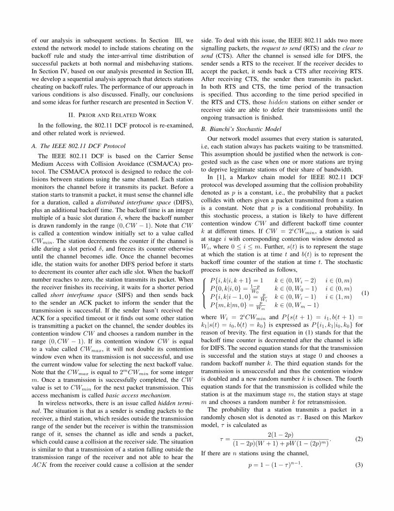
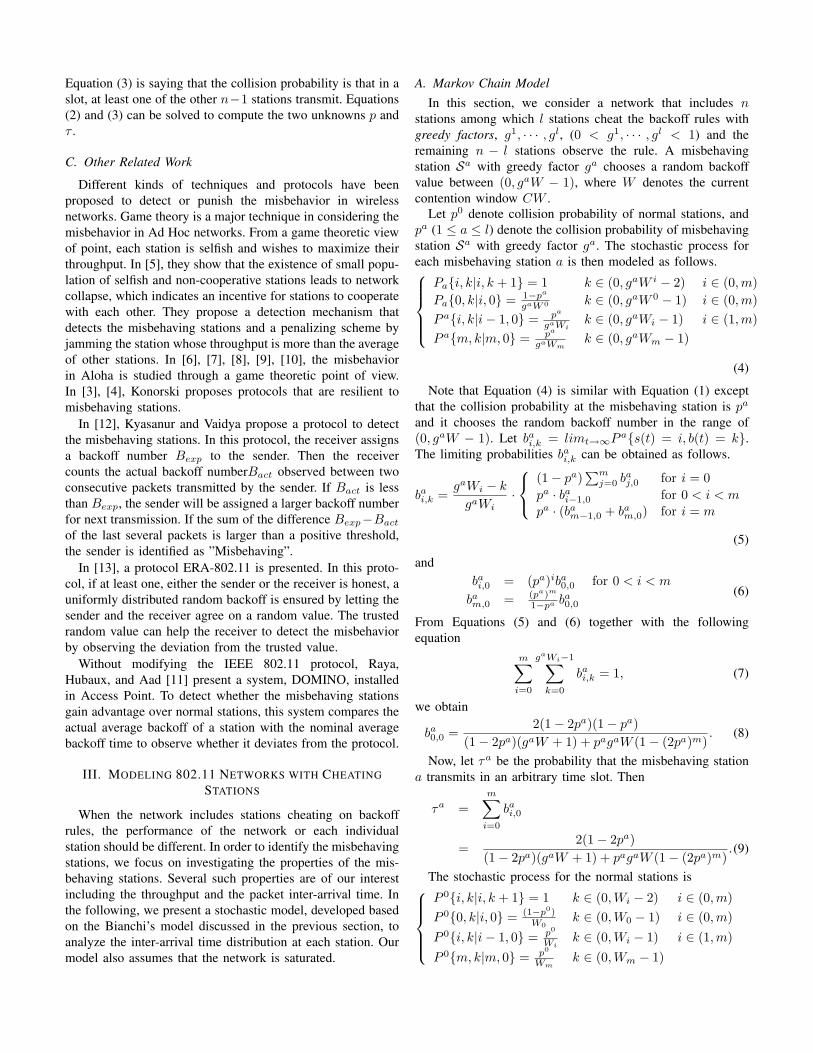
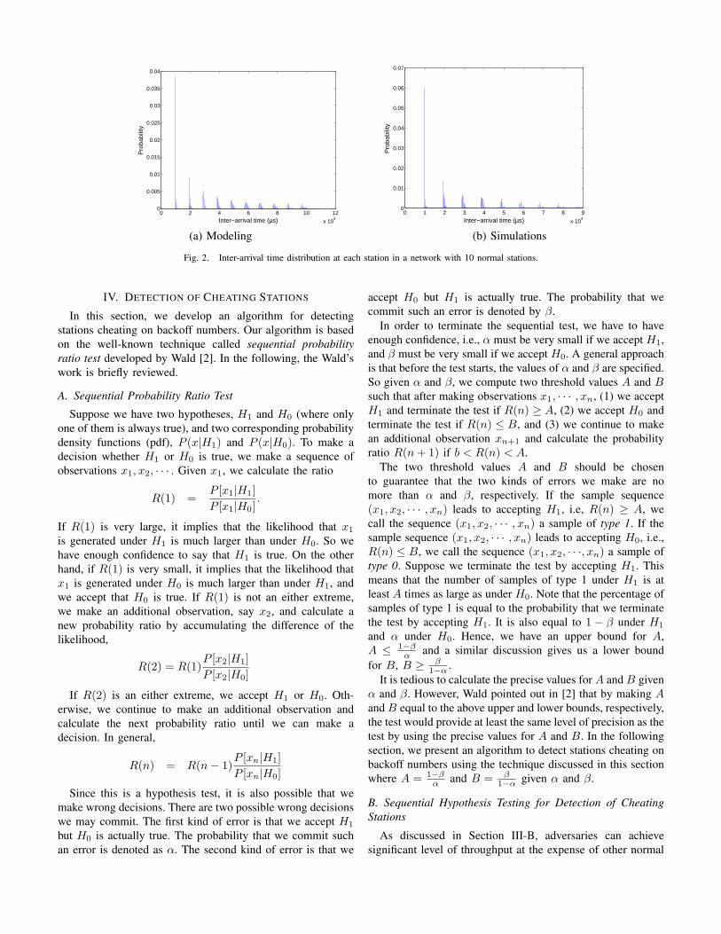
We first considered a network with 10 normal stations. Ta-ble II shows τ and p values computed from Equation (15) andobtained from simulations. Figure 2 shows the numerical andsimulation results of the packet inter-arrival time distribution ateach individual station. By conducting extensive simulations,we have observed that each of the 10 stations has almostidentical probability distribution of inter-arrival time.

Now we considered the network including 7 stations ob-serving the rule (i.e., with greedy factor 1.00) and 3 stations

TABLE IIτ AND p IN A NETWORK WITH 10 NORMAL STATIONS

Modeling Simulationg = 1.00 τ 0.0525 0.0565

p 0.3844 0.3651TABLE III

τ AND p IN A NETWORK WITH 7 NORMAL AND 3 CHEATING STATIONS

Modeling Simulationg = 0.25 τ 0.2358 0.2703

p 0.3269 0.2763g = 0.5 τ 0.0808 0.0968

p 0.4404 0.3982g = 0.75 τ 0.0502 0.0594

p 0.4584 0.4217g = 1 τ 0.0365 0.0425

p 0.4661 0.4340

cheating on the backoff rule with the greedy factor of eachstation being 0.25, 0.50, 0.75. So we have 8 variables tocompute obtained from Equation (15), which are shown inEquation (25) where station Si, for 0 ≤ i ≤ 3, has greedyfactor 1.00, 0.25, 0.50, and 0.75, respectively. Table III showsthese 8 values computed from Equation (15) using a numericalmethod.

τ0 = 2(1−2p0)(1−2p0)(W+1)+p0W (1−(2p0)m)

τ1 = 2(1−2p1)(1−2p1)(0.25W+1)+p1(0.25W )(1−(2p1)m)

τ2 = 2(1−2p2)(1−2p2)(0.5W+1)+p2(0.5W )(1−(2p2)m)

τ3 = 2(1−2p3)(1−2p3)(0.75W+1)+p3(0.75W )(1−(2p3)m)

p0 = 1− (1− τ1)(1− τ2)(1− τ3)(1− τ0)6

p1 = 1− (1− τ2)(1− τ3)(1− τ0)7

p2 = 1− (1− τ1)(1− τ3)(1− τ0)7

p3 = 1− (1− τ1)(1− τ2)(1− τ0)7

(25)

Figure 3 shows the numerical and simulation results of thepacket inter-arrival time distribution at each of the normal andmalicious stations. Again, the simulation results of all 7 normalstations are almost identical, and we only show the results ofone such a station.

Several important observations are made from our analyticaland simulation results.

• In regard to the packet inter-arrival time, each graph(from modeling or simulation) shows several peaks. Thefirst peak corresponds to the case that no other stationhas a packet successfully transmitted, i.e., T (i, k, s, f)with s = 0. The (s + 1)th peak in (a) or (b) of thefigure corresponds to the case that s packets have beensuccessfully transmitted by other stations.

• Stations cheating on the backoff rule can achieve higherthroughput as they have higher probabilities in lowervalues of packet inter-arrival times, which can draw aconclusion that monitoring packet inter-arrival times ateach station can provide significant information that canbe used in detecting such stations.

In the following section, we discuss how the results dis-cussed in this section can in fact lead to an interesting schemeto detect cheating stations.

0 2 4 6 8 10 12

x 104

0

0.005

0.01

0.015

0.02

0.025

0.03

0.035

0.04

Inter−arrival time (µs)

Pro

babi

lity

0 1 2 3 4 5 6 7 8 9

x 104

0

0.01

0.02

0.03

0.04

0.05

0.06

0.07

Inter−arrival time (µs)

Pro

babi

lity

(a) Modeling (b) Simulations

Fig. 2. Inter-arrival time distribution at each station in a network with 10 normal stations.

IV. DETECTION OF CHEATING STATIONS

In this section, we develop an algorithm for detectingstations cheating on backoff numbers. Our algorithm is basedon the well-known technique called sequential probabilityratio test developed by Wald [2]. In the following, the Wald’swork is briefly reviewed.

A. Sequential Probability Ratio Test

Suppose we have two hypotheses, H1 and H0 (where onlyone of them is always true), and two corresponding probabilitydensity functions (pdf), P (x|H1) and P (x|H0). To make adecision whether H1 or H0 is true, we make a sequence ofobservations x1, x2, · · · . Given x1, we calculate the ratio

R(1) =P [x1|H1]P [x1|H0]

.

If R(1) is very large, it implies that the likelihood that x1

is generated under H1 is much larger than under H0. So wehave enough confidence to say that H1 is true. On the otherhand, if R(1) is very small, it implies that the likelihood thatx1 is generated under H0 is much larger than under H1, andwe accept that H0 is true. If R(1) is not an either extreme,we make an additional observation, say x2, and calculate anew probability ratio by accumulating the difference of thelikelihood,

R(2) = R(1)P [x2|H1]P [x2|H0]

If R(2) is an either extreme, we accept H1 or H0. Oth-erwise, we continue to make an additional observation andcalculate the next probability ratio until we can make adecision. In general,

R(n) = R(n− 1)P [xn|H1]P [xn|H0]

Since this is a hypothesis test, it is also possible that wemake wrong decisions. There are two possible wrong decisionswe may commit. The first kind of error is that we accept H1

but H0 is actually true. The probability that we commit suchan error is denoted as α. The second kind of error is that we

accept H0 but H1 is actually true. The probability that wecommit such an error is denoted by β.

In order to terminate the sequential test, we have to haveenough confidence, i.e., α must be very small if we accept H1,and β must be very small if we accept H0. A general approachis that before the test starts, the values of α and β are specified.So given α and β, we compute two threshold values A and Bsuch that after making observations x1, · · · , xn, (1) we acceptH1 and terminate the test if R(n) ≥ A, (2) we accept H0 andterminate the test if R(n) ≤ B, and (3) we continue to makean additional observation xn+1 and calculate the probabilityratio R(n + 1) if b < R(n) < A.

The two threshold values A and B should be chosento guarantee that the two kinds of errors we make are nomore than α and β, respectively. If the sample sequence(x1, x2, · · · , xn) leads to accepting H1, i.e, R(n) ≥ A, wecall the sequence (x1, x2, · · · , xn) a sample of type 1. If thesample sequence (x1, x2, · · · , xn) leads to accepting H0, i.e.,R(n) ≤ B, we call the sequence (x1, x2, · · ·, xn) a sample oftype 0. Suppose we terminate the test by accepting H1. Thismeans that the number of samples of type 1 under H1 is atleast A times as large as under H0. Note that the percentage ofsamples of type 1 is equal to the probability that we terminatethe test by accepting H1. It is also equal to 1 − β under H1

and α under H0. Hence, we have an upper bound for A,A ≤ 1−β

α and a similar discussion gives us a lower boundfor B, B ≥ β

1−α .It is tedious to calculate the precise values for A and B given

α and β. However, Wald pointed out in [2] that by making Aand B equal to the above upper and lower bounds, respectively,the test would provide at least the same level of precision as thetest by using the precise values for A and B. In the followingsection, we present an algorithm to detect stations cheating onbackoff numbers using the technique discussed in this sectionwhere A = 1−β

α and B = β1−α given α and β.

B. Sequential Hypothesis Testing for Detection of CheatingStations

As discussed in Section III-B, adversaries can achievesignificant level of throughput at the expense of other normal

0 2 4 6 8 10

x 104

0

0.005

0.01

0.015

0.02

0.025

0.03

0.035

Inter−arrival time (µs)

Pro

babi

lity

0 1 2 3 4 5 6 7 8 9

x 104

0

0.01

0.02

0.03

0.04

0.05

0.06

0.07

Inter−arrival time (µs)

Pro

babi

lity

(a) Normal station (M) (b) Normal station (S)

0 2 4 6 8 10

x 104

0

0.005

0.01

0.015

0.02

0.025

0.03

0.035

0.04

0.045

Inter−arrival time (µs)

Pro

babi

lity

0 1 2 3 4 5 6 7 8 9

x 104

0

0.01

0.02

0.03

0.04

0.05

0.06

0.07

0.08

Inter−arrival time (µs)

Pro

babi

lity

(c) Station with g = 0.75 (M) (d) Station with g = 0.75 (S)

0 2 4 6 8 10

x 104

0

0.01

0.02

0.03

0.04

0.05

0.06

0.07

Inter−arrival time (µs)

Pro

babi

lity

0 2 4 6 8 10

x 104

0

0.01

0.02

0.03

0.04

0.05

0.06

0.07

Inter−arrival time (µs)

Pro

babi

lity

0 1 2 3 4 5 6 7 8 9

x 104

0

0.02

0.04

0.06

0.08

0.1

0.12

0.14

Inter−arrival time (µs)

Pro

babi

lity

(e) Station with g = 0.50 (M) (f) Station with g = 0.50 (S)

0 2 4 6 8 10

x 104

0

0.02

0.04

0.06

0.08

0.1

0.12

0.14

0.16

0.18

Inter−arrival time (µs)

Pro

babi

lity

0 1 2 3 4 5 6 7 8 9

x 104

0

0.05

0.1

0.15

0.2

0.25

Inter−arrival time (µs)

Pro

babi

lity

0 1 2 3 4 5 6 7 8 9

x 104

0

0.05

0.1

0.15

0.2

0.25

Inter−arrival time (µs)

Pro

babi

lity

(g) Station with g = 0.25 (M) (h) Station with g = 0.25 (S)

Fig. 3. Inter-arrival time distribution at each station in a network with 7 normal stations and 3 malicious stations, each with g = 0.75, 0.50, and 0.25.

stations by choosing smaller values of greedy factors whilemaintaining the randomness of the selection, hence hiding theirmalicious behaviors. In the following, based on the techniqueshown in sequential probability ratio test, we develop analgorithm detecting such malicious behavior.

1) Data Analysis: Our work is grounded using the packetinter-arrival time distribution and the throughput achieved ateach station under various scenarios (e.g., number of activestations, greedy factor used by each station, etc.). We note herethat if the network is not saturated, the impact of maliciousbehaviors by cheating backoff numbers may be ignorable,hence, we are only interested in the situation when the networkis saturated.

Note that in both simulation and our analytical model,the packet inter-arrival times are shown to be discrete, butin real situations, this may not be the case due to manyreasons such as signal dissipation during the transmission,variable packet lengths from time to time, etc. So, we simplifythe expressions of the distributions as P (t1 ≤ T < t2).In other words, we divide the time scale into smaller inter-vals, [t0, t1), [t1, t2), · · · [tk, tk+1) · · · . And we calculate theprobability of P (ti ≤ T < ti+1) for each station, whereP (ti ≤ T < ti+1) denotes the probability of the packet inter-arrival time being between ti and ti+1.

What would then be the reasonable time intervals withoutlosing any important characteristics of the inter-arrival time?Fortunately, the distributions calculated by both our model andsimulations show an interesting property: the burstiness. Notethat in Figure 2, for example, the first major peak correspondsto a set of inter-arrival times during which there are no othersuccessful transmissions made by any station. Similarly, thesecond major peak corresponds to a set of inter-arrival timesduring which there is exactly one successful transmissionby some other station. Therefore, the starting point of thesecond major peak is approximately 2Ts. The rest of the peaksmay be similarly interpreted. Within one major peak, whenthe inter-arrival time gets larger, the probability gets smaller,and the probability approaches to zero when approaching tothe next major peak. When falling into the next peak, theprobability first becomes large and then becomes smaller asthe corresponding inter-arrival time gets larger. In other words,the distribution of the inter-arrival times presents an excellentguideline for dividing the time scale. Therefore, we dividethe inter-arrival time into [0, Ts), [Ts, 2Ts), · · · , [kTs, (k +1)Ts) · · · .

To execute the sequential probability ratio test, we haveto know the distributions of the inter-arrival times under H1

and under H0. In other words, we have to know the exactgreedy factor of the misbehaving station. Such informationis not available in practice. It is even possible that we don’tknow whether there exists such a misbehaving station or not.Even more complicated, there may exist multiple misbehavingstations with different greedy factors. We first tackle theproblem that there exists only one misbehaving station in thenetwork, then move to the case that multiple misbehavingstations exist. To illustrate our approach, we first consider

a simple case that there is only one cheating station in thenetwork.

2) Single Cheating Station: We start with the simplestscenario that there is only one cheating station and its greedyfactor g0 < 1 is known. The problem is then to find outwhich station is the cheating station. Note that the greedyfactor of any normal station is 1. Then, the two hypothesescan be expressed as H1 being g = g0 and H0 being g = 1.For the ith observed inter-arrival time xi, if xi falls into thejth major peak, i.e., jTs ≤ xi < (j + 1)Ts, we denote theprobability P [jTs ≤ xi < (j + 1)Ts|H1] as P [Qj |H1], andP [jTs ≤ xi < (j + 1)Ts|H0] as P [Qj |H0]. Note that thevalues of P [Qj |H0] and P [Qj |H1] for each j are availablefrom real experiments.

Given the desired values of α and β, let A = 1−βα and

B = β1−α . Our algorithm works assuming that the packet

inter-arrival times xi of each suspicious station is monitored.The algorithm is described below.

Algorithm 01: i = 1. Pr = 1.2: Make the ith observation, calculate the inter-arrival time

xi, and find out the jth peak which xi falls into.3: Pr = Pr × P [Qj |H1]

P [Qj |H0];

4: If B < Pr < A, i ←− i + 1 and go to step 2.5: If Pr ≥ A, return H1 and terminate the algorithm.6: If Pr ≤ B, return H0 and terminate the algorithm.

Now, we move to a more complicated case that we knowthere exists only one misbehaving station but we don’t knowits greedy factor. For a suspicious station, we need to test thehypothesis H1 : g < 1 against the hypothesis H0 : g = 1.

We first observe the following fact. If the only misbehavingstation has g < g0, by applying the test H1 : g = g0 againstH0 : g = 1, the probabilities that we commit the first andsecond kind of error are less than α and β, respectively. Thereason is as follows. Consider two scenarios: (1) n−1 normalstations are coexisting with one cheating station with g = g0,(2) n − 1 normal stations are coexisting with one cheatingstation with g < g0, for a given value g0. As discussed before,for the scenario (1), by applying the hypothesis test H1 : g =g0 against H0 : g = 1, the probabilities that we commit thetwo kinds of errors are nearly α and β, respectively. Comparedwith the cheating station in the scenario (1), in the scenario (2),the cheating station with g < g0 should be more misbehaving,meaning that the station with g < g0 tends to send out itspackets after waiting for a shorter period. Hence, it has morepackets falling into the first several peaks, and less packetsfalling into those peaks corresponding to large inter-arrivaltimes. When we apply the hypothesis test H1 : g = g0 againstH0 : g = 1 on the station with g < g0, the algorithm speedsup and tends to terminate by accepting H1. In other words, theprobability of the second kind of error is smaller than whenapplying the H1 : g = g0 against H0 : g = 1 on the stationwith g = g0, which is nearly β. In general, the probability ofthe second kind of error decreases as g decreases in the domaing ≤ g0. Meanwhile, compared with the normal stations in

the scenario (1), in the scenario (2), the normal stations aremore normal. Because of the existence of the station withg < g0, the normal stations tend to send their packets aftera longer period. The normal stations have more inter-arrivaltimes falling into the peaks corresponding to large inter-arrivaltimes. When we apply the hypothesis test H1 : g = g0 againstH0 : g = 1 on the normal stations coexisting with station ofg < g0, the algorithm is more likely to terminate by acceptingH0. In general, as the g of the misbehaving station decreasesin the domain g ≤ g0, the probability of the first kind oferror decreases. So if we know the range of the misbehavingstation’s greedy factor g, say g < g0, we can apply thehypothesis test H1 : g = g0 against H0 : g = 1 accordingly tofind out the misbehaving station.

We can select g0 value by ourselves as long as we aresure that the selected g0 is larger than the real g of themisbehaving station. The g0 value may be a critical pointfor the network performance. For example, if there exists amisbehaving station with g = g0 = 0.565, the throughput ofa normal station is observed to decrease by 10% when thereare 9 normal stations. So, once we find the throughput of anormal station is decreased by at least 10%, which meansthat the misbehaving station must have g ≤ g0, we apply thehypothesis test H1 : g < g0 against H0 : g = 1. As discussedbefore, by applying this test on both misbehaving and normalstations, the probabilities of committing the two kinds of errorsare no more than α and β, respectively.

3) Multiple Cheating Stations: Now, consider the case thatamong the total n stations, l stations are misbehaving withgreedy factors, g1, · · · , gl, (0 < g1, · · · , gl < 1) but we don’tknow how many cheating stations in the network and we don’tknow their greedy factors. How should we then proceed toapply the hypothesis test?

As we mentioned before, we can choose g0 according to thethroughput of a normal station in the network. For example,we may think that 10% throughput degradation of a normalstation is intolerable. For each throughput degradation d%,for example d = 10, we calculate the following parameters.If there are totally n stations in the network, we calculate thegreedy factor value gd

i (1 ≤ i ≤ n − 1) such that if thereexist i misbehaving stations with the same greedy factor gd

i ,the throughput of a normal station decreases by d%. The gd

i

value can be obtained in advance through experiments (in ourcase through simulations). Then it is true that gd

1 < gd2 < · · · <

gdi < · · · < gd

n−1. This is because that if i misbehaving stationswith the greedy factors gd

i cause the throughput of a normalstation decreased by d%, by forcing one of the remaining n−inormal stations to be misbehaving with g = gd

i , the throughputof a normal station must be decreased by more than d%. Sogd

i+1 > gdi .

Once we find that the throughput of a normal stationdecreases by at least d%, we start with the hypothesis testH1 : g = gd

1 against H0 : g = 1, assuming that there isonly one misbehaving station. If there is only one misbehavingstation, the misbehaving station must have g ≤ gd

1 in orderto cause at least d% throughput degradation of a normal

station. By applying the hypothesis test H1 : g = gd1 against

H0 : g = 1, we can detect the misbehaving station as wediscussed before.

However, if there are more than one misbehaving stations,each misbehaving station does not have to have g as small asgd1 to cause d% throughput degradation of the network. For

example, if there are two misbehaving stations both with gd2

(g2 > g1), they can still make the throughput of a normalstation decreased by at least d%. The two stations with gd

2 ,compared with the case that a single cheating station existswith gd

1 , tend to have relatively larger inter-arrival times. Thus,when we apply the test H1 : g = gd

1 against H0 : g = 1 onthe two misbehaving stations, we may not be able to detectany of them. But if we apply the hypothesis H1 : g = gd

2

against H0 : g = 1, we can detect them using the distributionP (x|g = gd

2).Now, consider the case that the two cheating stations have

different greedy factors. If the throughput of a normal stationis decreased by at least d%, one misbehaving station must haveg ≤ gd

2 . The reason is that if both have g > gd2 , which means

that the two stations are not as harmful as the stations withg = gd

2 , the throughput degradation of a normal station mustbe less than d%. So when compared with the case that the twostations have the same g = gd

2 , the station with the smallestgreedy factor does more harm to the network. Therefore, whenwe apply the hypothesis test H1 : g = gd

2 against H0 : g = 1on the station with the smallest greedy factor, the test tendsto terminate by accepting H1 more quickly, which means thatthe second kind of error is smaller than β.

In general, if there are i misbehaving stations with differentgreedy factors, while throughput of a normal station is de-creased by at least d%, the station with the smallest greedyfactor g value must have g ≤ gd

i . Therefore, compared withi cheating stations with the same gd

i values, the station withthe smallest greedy factor among the i misbehaving stationstends to have smaller inter-arrival time. Thus, when applyingthe test H1 : g = gd

i against H0 : g = 1 on the station with thesmallest greedy factor among the i misbehaving stations, thetest tends to terminate more quickly by accepting H1. Thus,when testing the most misbehaving station, the probability thatwe accept it as normal is even smaller than β. For those normalstations, since their throughputs decrease by at least d%, theyare as least as normal as the normal stations coexisting withn− i misbehaving stations with the same g = gd

i . Thus, whenapplying the hypothesis test H1 : g = gd

i against H0 : g = 1on the normal stations, the probability that we commit the firstkind of error is bounded by α.

The overall idea of our approach works as follows. If wefind that the throughput of a normal station is decreased byat least d%, we first apply the test H1 : g = gd

1 against H0 :g = 1 assuming that there is only one misbehaving station. Ifwe can find any misbehaving station, then disable it. If not,which means that there may be multiple misbehaving stationswith relatively larger greedy factors, we move to use the testH1 : g = gd

2 against H0 : g = 1, by assuming that thereare two misbehaving stations. If we identify some stations as

misbehaving (i.e., we detect those stations with the smallestgreedy factors), disable the misbehaving stations, and checkwhether the throughput goes back to normal. If the throughputis still abnormal with the throughput degradation d′, we startthe procedure again by applying the test H1 : g = gd′

1 againstH0 : g = 1. If we can’t find any misbehaving station whenapplying the test H1 : g = gd

2 against H0 : g = 1, whichmeans that there are more than two misbehaving stationswith relatively larger greedy factors, we move to use the testH1 : g = gd

3 against H0 : g = 1. Keep doing the procedurethat if we can’t find any misbehaving station by applying thetest H1 : g = gd

i against H0 : g = 1, then move to thetest H1 : g = gd

i+1 against H0 : g = 1; if we find somemisbehaving stations, then disable them and check whether thethroughput goes back to normal. If after disabling the detectedmisbehaving stations, the throughput is still abnormal, we startthe procedure above again until we disable all misbehavingstations. During this procedure, we can guarantee that thedetected misbehaving stations have the smallest greedy factorsamong all misbehaving stations and for the station with thesmallest greedy factor, the probability that we accept it asnormal is smaller than β; for any real normal station, theprobability that we accept it as misbehaving is close to α.

A formal description of this approach is presented in thenext section.

C. Sequential Algorithm

Algorithm Sequential Hypothesis Testing Algo-rithm

1: For a specific d value, obtain a table that stores the valuegd

k,n such that if there are k(1 ≤ k ≤ n− 1) misbehavingstations out of n stations with the same greedy factorgd

k,n, the throughput of a normal station is decreased byd%. This can be done by experimenting in real situation(by simulating in our case) k misbehaving stations andchecking how much throughput of a normal station isdecreased. Then, for each station, calculate the probabilityof the inter-arrival time x, P [jTs ≤ x < (j + 1)Ts|g =gd

k,n] = P [Qj |g = gdk,n], and for one of the n− k normal

stations, calculate the probability of the inter-arrival timex, P [jTs ≤ x < (j + 1)Ts|g = 1] = P [Qj |g = 1] basedon the monitoring of packet inter-arrival times.

2: In the network with n working stations, roughly estimatewhether the throughput of a normal station is decreasedby at least d%.

3: k = 1. For each suspicious station, apply the algorithmDetect(k, n, d). If Detect(k, n, d) terminates by accept-ing some stations as misbehaving, remove the misbehav-ing ones from the network and go back to step 2. IfDetect(k, n, d) didn’t find any misbehaving station, k ←−k + 1 and for each suspicious station do Detect(k, n, d).

Algorithm Detect(k, n, d)1: i = 1. Pr = 1.2: Make the ith observation, calculate the inter-arrival time

xi, and find out the jth peak which xi falls into. Obtain

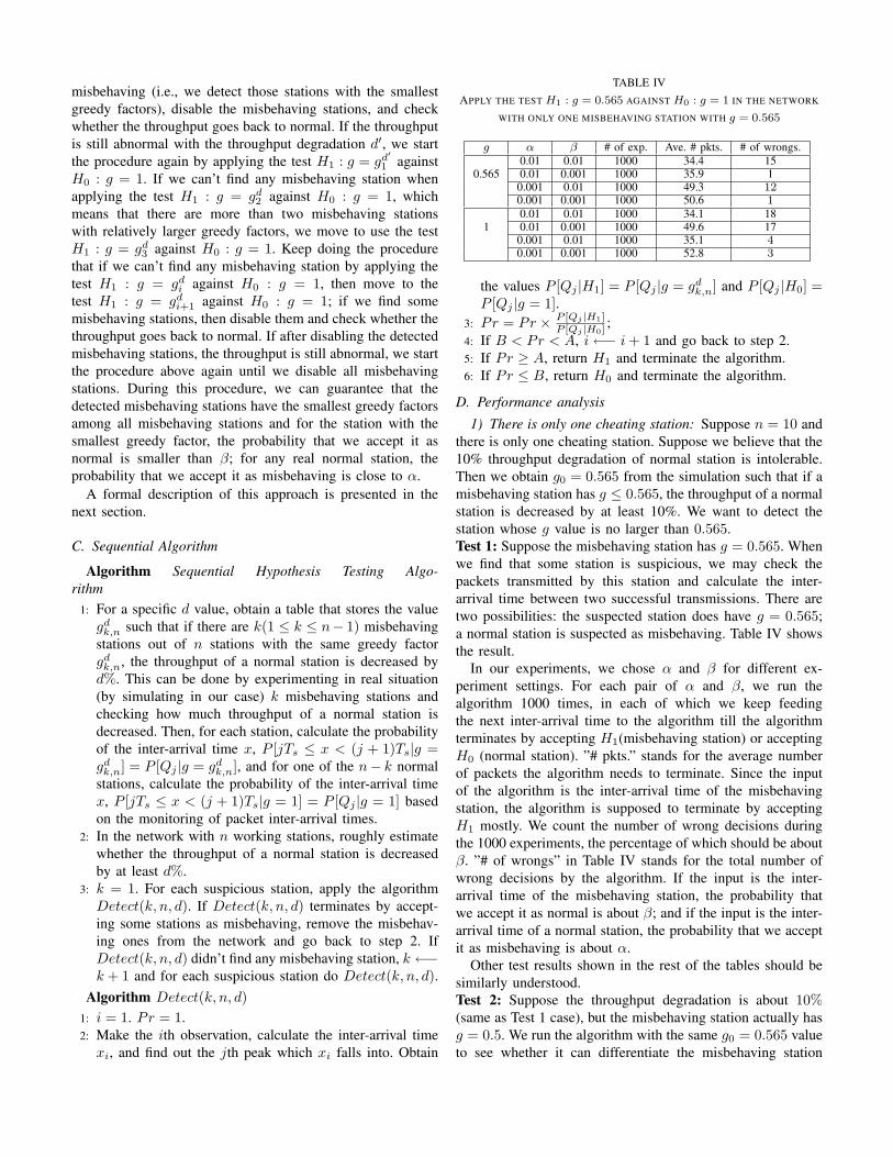
TABLE IVAPPLY THE TEST H1 : g = 0.565 AGAINST H0 : g = 1 IN THE NETWORK

WITH ONLY ONE MISBEHAVING STATION WITH g = 0.565

g α β # of exp. Ave. # pkts. # of wrongs.0.01 0.01 1000 34.4 15

0.565 0.01 0.001 1000 35.9 10.001 0.01 1000 49.3 120.001 0.001 1000 50.6 10.01 0.01 1000 34.1 18

1 0.01 0.001 1000 49.6 170.001 0.01 1000 35.1 40.001 0.001 1000 52.8 3

the values P [Qj |H1] = P [Qj |g = gdk,n] and P [Qj |H0] =

P [Qj |g = 1].3: Pr = Pr × P [Qj |H1]

P [Qj |H0];

4: If B < Pr < A, i ←− i + 1 and go back to step 2.5: If Pr ≥ A, return H1 and terminate the algorithm.6: If Pr ≤ B, return H0 and terminate the algorithm.

D. Performance analysis

1) There is only one cheating station: Suppose n = 10 andthere is only one cheating station. Suppose we believe that the10% throughput degradation of normal station is intolerable.Then we obtain g0 = 0.565 from the simulation such that if amisbehaving station has g ≤ 0.565, the throughput of a normalstation is decreased by at least 10%. We want to detect thestation whose g value is no larger than 0.565.Test 1: Suppose the misbehaving station has g = 0.565. Whenwe find that some station is suspicious, we may check thepackets transmitted by this station and calculate the inter-arrival time between two successful transmissions. There aretwo possibilities: the suspected station does have g = 0.565;a normal station is suspected as misbehaving. Table IV showsthe result.

In our experiments, we chose α and β for different ex-periment settings. For each pair of α and β, we run thealgorithm 1000 times, in each of which we keep feedingthe next inter-arrival time to the algorithm till the algorithmterminates by accepting H1(misbehaving station) or acceptingH0 (normal station). ”# pkts.” stands for the average numberof packets the algorithm needs to terminate. Since the inputof the algorithm is the inter-arrival time of the misbehavingstation, the algorithm is supposed to terminate by acceptingH1 mostly. We count the number of wrong decisions duringthe 1000 experiments, the percentage of which should be aboutβ. ”# of wrongs” in Table IV stands for the total number ofwrong decisions by the algorithm. If the input is the inter-arrival time of the misbehaving station, the probability thatwe accept it as normal is about β; and if the input is the inter-arrival time of a normal station, the probability that we acceptit as misbehaving is about α.

Other test results shown in the rest of the tables should besimilarly understood.Test 2: Suppose the throughput degradation is about 10%(same as Test 1 case), but the misbehaving station actually hasg = 0.5. We run the algorithm with the same g0 = 0.565 valueto see whether it can differentiate the misbehaving station

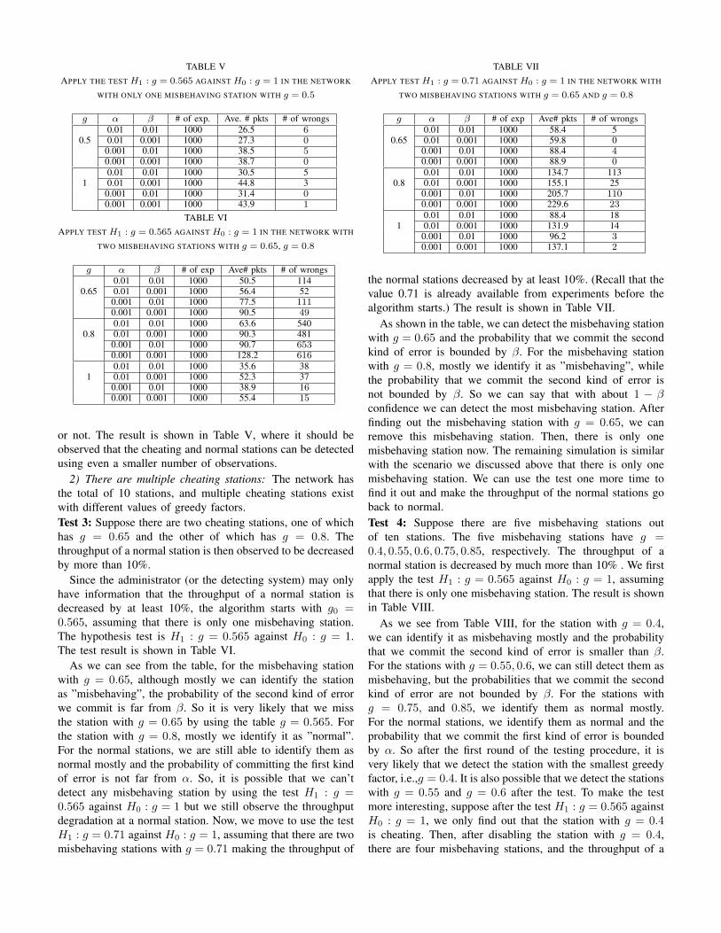
TABLE VAPPLY THE TEST H1 : g = 0.565 AGAINST H0 : g = 1 IN THE NETWORK

WITH ONLY ONE MISBEHAVING STATION WITH g = 0.5

g α β # of exp. Ave. # pkts # of wrongs0.01 0.01 1000 26.5 6

0.5 0.01 0.001 1000 27.3 00.001 0.01 1000 38.5 50.001 0.001 1000 38.7 00.01 0.01 1000 30.5 5

1 0.01 0.001 1000 44.8 30.001 0.01 1000 31.4 00.001 0.001 1000 43.9 1

TABLE VIAPPLY TEST H1 : g = 0.565 AGAINST H0 : g = 1 IN THE NETWORK WITH

TWO MISBEHAVING STATIONS WITH g = 0.65, g = 0.8

g α β # of exp Ave# pkts # of wrongs0.01 0.01 1000 50.5 114

0.65 0.01 0.001 1000 56.4 520.001 0.01 1000 77.5 1110.001 0.001 1000 90.5 490.01 0.01 1000 63.6 540

0.8 0.01 0.001 1000 90.3 4810.001 0.01 1000 90.7 6530.001 0.001 1000 128.2 6160.01 0.01 1000 35.6 38

1 0.01 0.001 1000 52.3 370.001 0.01 1000 38.9 160.001 0.001 1000 55.4 15

or not. The result is shown in Table V, where it should beobserved that the cheating and normal stations can be detectedusing even a smaller number of observations.

2) There are multiple cheating stations: The network hasthe total of 10 stations, and multiple cheating stations existwith different values of greedy factors.Test 3: Suppose there are two cheating stations, one of whichhas g = 0.65 and the other of which has g = 0.8. Thethroughput of a normal station is then observed to be decreasedby more than 10%.

Since the administrator (or the detecting system) may onlyhave information that the throughput of a normal station isdecreased by at least 10%, the algorithm starts with g0 =0.565, assuming that there is only one misbehaving station.The hypothesis test is H1 : g = 0.565 against H0 : g = 1.The test result is shown in Table VI.

As we can see from the table, for the misbehaving stationwith g = 0.65, although mostly we can identify the stationas ”misbehaving”, the probability of the second kind of errorwe commit is far from β. So it is very likely that we missthe station with g = 0.65 by using the table g = 0.565. Forthe station with g = 0.8, mostly we identify it as ”normal”.For the normal stations, we are still able to identify them asnormal mostly and the probability of committing the first kindof error is not far from α. So, it is possible that we can’tdetect any misbehaving station by using the test H1 : g =0.565 against H0 : g = 1 but we still observe the throughputdegradation at a normal station. Now, we move to use the testH1 : g = 0.71 against H0 : g = 1, assuming that there are twomisbehaving stations with g = 0.71 making the throughput of

TABLE VIIAPPLY TEST H1 : g = 0.71 AGAINST H0 : g = 1 IN THE NETWORK WITH

TWO MISBEHAVING STATIONS WITH g = 0.65 AND g = 0.8

g α β # of exp Ave# pkts # of wrongs0.01 0.01 1000 58.4 5

0.65 0.01 0.001 1000 59.8 00.001 0.01 1000 88.4 40.001 0.001 1000 88.9 00.01 0.01 1000 134.7 113

0.8 0.01 0.001 1000 155.1 250.001 0.01 1000 205.7 1100.001 0.001 1000 229.6 230.01 0.01 1000 88.4 18

1 0.01 0.001 1000 131.9 140.001 0.01 1000 96.2 30.001 0.001 1000 137.1 2

the normal stations decreased by at least 10%. (Recall that thevalue 0.71 is already available from experiments before thealgorithm starts.) The result is shown in Table VII.

As shown in the table, we can detect the misbehaving stationwith g = 0.65 and the probability that we commit the secondkind of error is bounded by β. For the misbehaving stationwith g = 0.8, mostly we identify it as ”misbehaving”, whilethe probability that we commit the second kind of error isnot bounded by β. So we can say that with about 1 − βconfidence we can detect the most misbehaving station. Afterfinding out the misbehaving station with g = 0.65, we canremove this misbehaving station. Then, there is only onemisbehaving station now. The remaining simulation is similarwith the scenario we discussed above that there is only onemisbehaving station. We can use the test one more time tofind it out and make the throughput of the normal stations goback to normal.Test 4: Suppose there are five misbehaving stations outof ten stations. The five misbehaving stations have g =0.4, 0.55, 0.6, 0.75, 0.85, respectively. The throughput of anormal station is decreased by much more than 10% . We firstapply the test H1 : g = 0.565 against H0 : g = 1, assumingthat there is only one misbehaving station. The result is shownin Table VIII.

As we see from Table VIII, for the station with g = 0.4,we can identify it as misbehaving mostly and the probabilitythat we commit the second kind of error is smaller than β.For the stations with g = 0.55, 0.6, we can still detect them asmisbehaving, but the probabilities that we commit the secondkind of error are not bounded by β. For the stations withg = 0.75, and 0.85, we identify them as normal mostly.For the normal stations, we identify them as normal and theprobability that we commit the first kind of error is boundedby α. So after the first round of the testing procedure, it isvery likely that we detect the station with the smallest greedyfactor, i.e.,g = 0.4. It is also possible that we detect the stationswith g = 0.55 and g = 0.6 after the test. To make the testmore interesting, suppose after the test H1 : g = 0.565 againstH0 : g = 1, we only find out that the station with g = 0.4is cheating. Then, after disabling the station with g = 0.4,there are four misbehaving stations, and the throughput of a

TABLE VIIIIN THE NETWORK WITH FIVE MISBEHAVING STATIONS,APPLY THE TEST

H1 : g = 0.565 AGAINST H0 : g = 1

g α β # of exp Ave# pkts # of wrongs0.01 0.01 1000 19.7 1

0.4 0.01 0.001 1000 20.1 00.001 0.01 1000 29.0 00.001 0.001 1000 29.1 00.01 0.01 1000 41.7.7 30

0.55 0.01 0.001 1000 44.2 40.001 0.01 1000 64.4 340.001 0.001 1000 68.4 30.01 0.01 1000 52.3 199

0.6 0.01 0.001 1000 64.1 880.001 0.01 1000 81.4 1910.001 0.001 1000 97.6 800.01 0.01 1000 49.7 872

0.75 0.01 0.001 1000 68.1 8890.001 0.01 1000 50.4 9610.001 0.001 1000 76.3 9560.01 0.01 1000 37.4 951

0.85 0.01 0.001 1000 55.3 9530.001 0.01 1000 40.44 9920.001 0.001 1000 58.8 9980.01 0.01 1000 23.7 5

1 0.01 0.001 1000 35.5 20.001 0.01 1000 24.9 00.001 0.001 1000 35.0 0

TABLE IXIN THE NETWORK WITH FOUR MISBEHAVING STATIONS, APPLY THE TEST

H1 : g = 0.6 AGAINST H0 : g = 1

g α β # of exp Ave# pkts # of wrongs0.01 0.01 1000 37.2 8

0.55 0.01 0.001 1000 36.4 00.001 0.01 1000 50.5 40.001 0.001 1000 54.9 00.01 0.01 1000 46.4 43

0.6 0.01 0.001 1000 51.2 70.001 0.01 1000 64.4 420.001 0.001 1000 73.4 60.01 0.01 1000 63.6 654

0.75 0.01 0.001 1000 97.2 6260.001 0.01 1000 94.0 7670.001 0.001 1000 131.7 7070.01 0.01 1000 48.9 878

0.85 0.01 0.001 1000 74.6 8940.001 0.01 1000 57.8 9360.001 0.001 1000 86.9 9460.01 0.01 1000 33.8 9

1 0.01 0.001 1000 48.8 80.001 0.01 1000 33.7 10.001 0.001 1000 50.6 1

normal station is still decreased by more than 10%. Supposewe have known in advance that in the network with 9 stations,if a station with g ≤ 0.6, the throughput of other eight normalstations will be decreased by at least 10%. So we start withthe test H1 : g = 0.6 against H0 : g = 1, assuming thatthere is only one misbehaving station. The result is shown inTable IX.

In Table IX, we can detect the most misbehaving stationwith g = 0.55 by using the test, while the probability ofcommitting the second kind of error is bounded by β for themost misbehaving station. And for the normal stations, we canidentify them as normal, while the probability that we commit

the first kind of error is bounded by α. Disable the stationwith g = 0.55, check the throughput of a normal station andcontinue this procedure similarly. Each time we can guaranteethat we are able to detect the station with the smallest greedyfactor and the probability that we identify the normal stationsas misbehaving is about or smaller than α.

V. CONCLUSION

We have presented the development and evaluation ofa sequential hypothesis testing algorithm applied to detectcheating stations in the IEEE 802.11 networks. The basisof our algorithm derives from the theory of the sequentialprobability ratio test introduced by Wald, which motivatesus to develop the analytical model of packet inter-arrivaldistribution at each station in the network under DoS attacks.Based on the throughput degradation monitored at a normalstation, algorithm parameters are dynamically selected forrunning the test. Simulation results show that our proposedscheme performs significantly fast and also accurately.

REFERENCES

[1] Giuseppe Bianchi, ”Performance Analysis of the IEEE 802.11 DistributedCoordination Function,” IEEE Journal on Selected Areas in Communica-tions., vol. 18, no.3, March 2000.

[2] Abraham Wald, Sequential Analysis, J. Wiley & Sons, New York, 1947.[3] J. Konorski, ”Protection of Fairness for Multimedia Traffic Streams in

a Non-cooperative Wireless LAN Setting,” In PROMS., volume 2213 ofLNCS. Springer, 2001.

[4] J. Konorski, ”Multiple Access in Ad-Hoc Wireless LANs with Nonco-operative Stations. In NETWORKING, volume 2345 of LNCS. Springer,2002.

[5] M. Cagalj, S. Ganeriwal, I. Aad and J.-P. Hubaux, ”On Selfish Behaviorin CSMA/CA Networks,” in Proceedings of the IEEE INFOCOM, 2005.

[6] A.B. MacKenzie and S. B. Wicher, ”Stability of Multipacket SlottedAloha with Selfish Users and Perfect Information,” in Proceedings ofthe IEEE INFOCOM, 2003.

[7] E. Altman, R.E.Azouzi, and T. Jimenes, Slotted Aloha as a StochasticGame with Partial Information”, in Proceedings of WiOpt, 2003.

[8] A.B. MacKenzie and S. B. Wicher, ”Selfish Users in Aloha: A gametheoretic approach,” in Proc. of the Fall 2001 IEEE Vehicular TechnologyConference (VTC Fall’01), 2001

[9] A.B. MacKenzie and S. B. Wicher, ”Game Theory and the Design ofSelf-Configuring, Adaptive Wireless Networks”, IEEE Commun. Mag.,2001.

[10] Y. Jin and G. Kesidis, ”Equilibria of a Noncoperative Game for Het-erogeneous Users of an ALOHA Network,” IEEE Comm. Letters, vol. 6,2002.

[11] M. Raya, J.-P Hubaux, and I. Aad, ”Domino: A System to DetectGreedy Behavior in IEEE 802.11 Hotspots,” in Proceedings of the SecondInternational Conference on Mobile Systems, Applicaitons and Services(MobiSys2004), Boston, Massachussets, June 2004.

[12] P. Kyasanur and N. Vaidya, ”Detection and Handling of MAC Layer-Misbehavior in Wireless Networks,” in Proceedings of the InternationalCOnference on Dependable Systems and Networks, June 2003.

[13] A.A. Cardenas, S.Radosavac and J.S. Baras, ”Detection and Preventionof MAC Layer Misbehavior in Ad Hoc Networks,” in SASN ’04:Proceedings of the 2nd ACM workshop on Security of ad hoc and sensornetworks, Washington DC, 2004.

[14] IEEE Standard for Wireless LAN MEdium Access Control (MAC) andPhysical Layer (PHY) Specifications, Nov. 1977. P802.11

[15] ns-2 Network Simulator. http://www.isi.edu/nsnam/ns/.