DETECTING SHIFT AND PURE CONTAGION IN EAST ASIAN EQUITY MARKETS: A UNIFIED APPROACH

Institute for International Integration Studies

IIIS Discussion Paper

No.236/ December 2007

Detecting Shift and Pure Contagion in East Asian EquityMarkets: A Unified Approach

Thomas J. Flavin Department of Economics, NUI Maynooth, Ireland

Ekaterini PanopoulouDepartment of Statistics and Insurance Science, Universityof Piraeus, Greece

IIIS Discussion Paper No. 236

Detecting Shift and Pure Contagion in East Asian Equity Markets: A Unified Approach

Thomas J. Flavin Ekaterini Panopoulou

Disclaimer Any opinions expressed here are those of the author(s) and not those of the IIIS. All works posted here are owned and copyrighted by the author(s). Papers may only be downloaded for personal use only.

Detecting shift and pure contagion in East Asian equity markets: A Unified Approach

Thomas J. Flavina,* , Ekaterini Panopouloub

a Department of Economics, NUI Maynooth, Maynooth, Co. Kildare, Ireland

b Department of Statistics and Insurance Science, University of Piraeus, Greece

This version: 29 October 2007 Abstract

We test for contagion between pairs of East Asian equity markets over the period 1990-2007. We develop an econometric methodology that allows us to test for both ‘shift’ and ‘pure’ contagion within a unified framework. Using both Hong Kong and Thailand as potential shock sources, we find strong evidence of both types of contagion. Therefore during episodes of high-volatility, equity returns are influenced by changes in the transmission of common shocks and additionally by the diffusion of idiosyncratic shocks through linkages which do not exist during normal times. Keywords: Shift contagion; Pure contagion; Financial market crises; Regime switching JEL Classification: F42; G15; C32

* Corresponding author. Tel.: +353 1 7083369; fax: +353 1 7083934. Email addresses: [email protected] (T.J. Flavin), [email protected] (E. Panopoulou).

1

1. Introduction

The equity markets of East Asia have suffered many episodes of turbulence

over the past two decades. Many of these events have been extreme and pervasive as

in the 1997-98 crisis period, while others have been less widespread but still represent

major downturns in equity returns. Frequently, these adverse shocks appear to exert

excessive influence on neighboring markets given existing levels of interdependence.

This has led many commentators to conclude that these simultaneous severe

experiences have been due to financial market contagion. However, in more recent

times, the issue of the existence and prevalence of contagion has become contentious,

with many contributors to the debate questioning whether contagion actually occurred

during the crisis.

The goal of our paper is to examine if contagion characterizes the behavior of

East Asian equity markets over the past two decades. Furthermore, we test for two

distinct channels of contagion within a unified framework. The extant literature tends

to distinguish between ‘shift’ and ‘pure’ contagion. Shift contagion occurs when the

interdependencies between pairs of markets increase during a crisis. The normal level

of interdependence may be due to pre-existing market linkages such as goods trade,

financial flows and other economic connections or exposure to common shocks. The

presence of shift contagion between markets implies that this existing or ‘normal’

relationship between market pairs becomes unstable during an episode of high-

volatility. On the other hand, pure contagion reflects excess contagion suffered during

a crisis that is not explained by market fundamentals or common shocks. Such

contagion is due to idiosyncratic shocks being transmitted to other countries through

2

channels that could not have been identified before the event.1 It is important to

correctly identify the type of contagion that is present in markets before prescribing

policy to deal with it. For example, if markets decline due to the effects of pure

contagion, then policies such as capital controls aimed at breaking market linkages are

unlikely to be successful. A better strategy would be to introduce policies aimed at

reducing country specific risks. We extend the methodology of Gravelle et al. (2006,

henceforth GKM) to facilitate tests for both types of contagion within a bivariate

regime-switching model in which both common and idiosyncratic shocks move

between low- and high-volatility states.

Whether or not the 1997-98 Asian crisis period was characterized by

contagion in equity markets has already attracted much attention but there is little

concensus in the reported results. For example, Forbes and Rigobon (2002) reject the

hypothesis that correlation coefficients between markets increased significantly

during the crisis period, leading the authors to conclude that there was ‘no contagion,

only interdependence’. Rigobon (2003b) fails to find evidence of a structural break in

the propagation of shocks. These papers find no evidence for either shift or pure

contagion. Likewise, Bordo and Murshid (2000) fail to find evidence in favor of

contagion during this crisis. In contrast, Caporale et al. (2003), Bekaert et al. (2005),

Bond et al. (2006) and Chiang et al. (2007), using a variety of techniques, all find

evidence of contagion between many pairs of Asian markets.2

We re-examine the issue using a framework capable of detecting both types of

contagion. We once again focus on equity markets within the region as a comparison

of results from Dungey et al. (2003, 2004) suggests that the impact of contagion on

1 For an overview of the various definitions of contagion, see Pericoli and Sbracia (2003) and Dungey and Tambakis (2005). 2 For a more complete review of the literature, the reader is referred to Dungey et al. (2006) and references therein.

3

return variation is more important for equity rather than currency markets. We don’t

focus exclusively on measuring contagion during the crisis of 1997-98, rather we

analyze whether or not contagion is a feature of high-volatility regimes over the past

two decades. Ito and Hashimoto (2005) document many episodes of turbulence over

this period for Asian equity markets. A desirable consequence of this approach is that

our analysis does not suffer from the common problem of having very small crisis

samples, often leading to low power in the tests being used (Dungey et al., 2007).

Even with weekly data, we have sufficient observations in both low- and high-

volatility regimes to classify them sharply.

Our paper is organized as follows. Section 2 presents our model. Section 3

describes the data and presents our empirical findings and the tests for contagion

using Hong Kong as the potential source of contagious effects. Section 4 presents a

robustness check using Thailand as the source country rather than Hong Kong.

Section 5 summarizes our empirical findings and offers some policy implications.

2. Econometric Methodology

We extend the methodology of GKM (2006) to test for both shift and pure

contagion within a unified framework. Their original model is developed to test for

shift contagion, and thus allows us to analyze the interdependence between two stock

markets during both calm and turbulent periods. We extend the model to capture the

potential effects of pure contagion whereby country-specific shocks are transmitted to

another market during episodes of high-volatility, through channels that are

unidentifiable during normal times.

The model is bivariate in nature and belongs to the family of factor models

widely used in financial economics. In this application, the factor model is attractive

4

in that we don’t have to enter the debate as to what the ‘fundamentals’ should be (see

Karolyi, 2003). The model can be summarized as follows. Let tr1 and tr2 represent

stock market returns from countries 1 and 2, respectively. Returns can be decomposed

into an expected, ,iµ and an unexpected component, itu , reflecting the arrival of

news to financial markets, i.e.

.0),( and 2,1,0)(, 21 ≠==+= ttititiit uuEiuEur µ (1)

The forecast errors are allowed to be contemporaneously correlated, implying that

common structural shocks may potentially be driving both returns. Therefore, we

decompose the forecast errors into two structural shocks, one idiosyncratic and one

common. Let 2,1, and =izz itct denote the common and idiosyncratic common

shocks respectively and let their impacts on asset returns be 2,1, and =iitcit σσ . Then

the forecast errors are written as:

.2,1, =+= izzu ititctcitit σσ (2)

Furthermore, their variances are normalized to unity, which means the impact

coefficients may be interpreted as the standard deviations of the shock.

Following GKM we allow both the common and the idiosyncratic shocks to

switch between two states – high- and low-volatility.3 With this structure in place,

each country return can move between four distinct regimes. The structural impact

coefficients 2,1,, =ictit σσ are given by the following:

2,1 ,)1(

2,1 ,)1(

=+−=

=+−=∗

∗

iSS

iSS

ctcictcicit

itiitiit

σσσ

σσσ (3)

where ciSit ,2,1),1,0( == are state variables that take the value of zero in normal

and unity in turbulent times. Variables with an asterisk belong to the high-volatility

3 The heteroskedasticity inherent in the structural shocks ensures the identification of the system (see also Rigobon, 2003a). As argued by GKM, only the assumption of regime switching in the common shocks is necessary for this. For further details of the identification process, please see GKM.

5

regime. To complete the model, we need to specify the evolution of regimes over

time. Following the regime-switching literature, the regime paths are Markov

switching and consequently are endogenously determined. Specifically, the

conditional probabilities of remaining in the same state, i.e. not changing regime are

defined as follows:

cipSSciqSS

iitit

iitit

,2,1,]1|1[Pr,2,1,]0|0[Pr

========

(4)

Furthermore, we relax the assumption of expected constant returns in (1).

These are allowed to be time varying and depend on the state of the common shock.4

In this respect, our model suggests that part of the stock market return represents a

risk premium that changes with the level of volatility.5 In particular, expected returns

are modeled as follows:

2,1 ,)1( =+−= ∗ iSS ctictiit µµµ (5)

Given that idiosyncratic shocks are uncorrelated with common shocks and mainly

associated with diversifiable risk, expected returns are not allowed to vary with the

volatility state of these shocks.

Finally, in an extension to the GKM (2006) model, we allow for the possibility

that the idiosyncratic shock of the source country exerts an influence on the other

country over and above that captured by the common shock. This is what we call pure

contagion and it’s captured by augmenting the return equation of country 2 with the

idiosyncratic shock of country 1 during the crisis period (see Dungey et al., 2005 for a

similar approach to capturing pure contagion).

4 Guidolin and Timmermann (2005) find that returns are statistically different across regimes though Ang and Bekaert (2002) fail to reject the equality of mean returns between regimes. 5 GKM also relax this assumption when modeling the interdependence of bond returns.

6

Though, the entire model is estimated in a single step, it implies different

features of the model in each of the possible regimes. For example, if we take the

extreme states, the characteristics of the model during tranquil periods (all shocks in

the low-volatility states) are given as follows.

tctct

tctct

zzrzzr

22222

11111

σσµσσµ++=++=

(6)

The two idiosyncratic shocks are assumed to be independent, so co-movements in

returns are solely determined by the common shock (factor). Thus, the variance-

covariance matrix of returns is given by:

++

=Σ 22

2221

2121

21

1ccc

ccc

σσσσσσσσ

.

On the other hand, during crisis periods (all shocks in high-volatility states),

the corresponding return generating process during periods of turbulence is given by

ttctct

tctct

zzzr

zzr

1*12

*2

*2

*22

1*1

*1

*11

δσσσµ

σσµ

+++=

++= (7)

The variance covariance matrix of returns is:

+++++

=Σ 2*1

22*2

2*2

2*1

*2

*1

2*1

*2

*1

2*1

2*1

8 σδσσδσσσδσσσσσ

ccc

ccc .

An extra assumption of normality of the structural shocks enables us to

estimate the full model given by equations (1)-(7) via maximum likelihood along the

lines of the methodology for Markov-switching models (see Hamilton, 1989).

2.1 Testing for shift contagion.

Our rationale behind testing for shift contagion (see also GKM) lies on

the assumption, that in its absence, a large unexpected shock that affects both

countries does not change their interdependence. In other words, the observed

7

increase in the variance and correlation of returns during crisis periods is due to

increased impulses stemming from the common shocks and not from changes in the

propagation mechanism of shocks. To empirically test for contagion, we conduct

hypothesis testing specifying the null and the alternative as follows:

2

1

2

11

2

1

2

10 : versus:

c

c

c

c

c

c

c

c HHσσ

σ

σσσ

σ

σ≠=

∗

∗

∗

∗ (8)

The null hypothesis postulates that in the absence of shift contagion, the impact

coefficients in both calm and crisis periods should move proportionately. This

likelihood ratio test is the common test for testing restrictions among nested models

and follows a 2χ distribution with one degree of freedom corresponding to the

restriction of equality of the ratio of coefficients between the two regimes.

2.2. Testing for pure contagion.

The final term in the return generating process of country 2 during the

turbulent period measures the impact of the other country’s shock on its return and

hence, measures the effect of pure contagion. This term only exerts an influence when

the idiosyncratic shock of the source country is in the high-volatility regime, as in all

other cases, σ1* = 0. Now, our test for pure contagion is a simple t-test on the

coefficient δ, where under the null δ=0 and there is no pure contagion.

3. Empirical Results

3.1. Data

Our dataset comprises weekly closing stock market indices from nine East

Asian countries: Japan, Korea, Indonesia, Malaysia, the Philippines, Singapore,

Taiwan, Thailand and Hong Kong. All indices are value-weighted, expressed in US

8

dollars and were obtained from Datastream International. The Datastream codes for

stock market indices have the following structure: TOTMKXX, where XX represents

the country code, i.e. JP (Japan), KO (Korea), ID (Indonesia), MY (Malaysia), PH

(Philippines), SG (Singapore), TA (Taiwan), TH (Thailand) and HK (Hong Kong).

The indices span a period of over 17 years from 4 April 1990 to 13 September 2007, a

total of 910 observations. Conducting the analysis with US dollar denominated returns

allows us to isolate equity market shocks. Moreover, we prefer weekly return data to

higher frequency data, such as daily returns, in order to account for any non-

synchronous trading in the countries under examination.6 For each index, we compute

the return between two consecutive trading periods, t-1 and t as ln(pt)- ln(pt-1) where pt

denotes the closing index on week t.

[TABLE 1 ABOUT HERE]

Table 1 (Panel A) presents descriptive statistics for the weekly returns, while

Panel B provides some preliminary evidence on the cross-country return correlation

structure. Mean returns vary considerably across countries, ranging from 0.063% in

Japan to 0.292% in Hong Kong. Korea and Indonesia were the most volatile over this

period while the Singaporean market appears to be the least volatile. The Jarque-Bera

test rejects normality for all markets, which is usual in the presence of both skewness

and excess kurtosis. Specifically, return distributions are negatively skewed for half

the countries with Singapore being the most skewed. On the other hand, the most

positively skewed return is Indonesia followed by the Philippines, Malaysia and

Japan. Indonesian and Malaysian returns exhibit considerable leptokurtosis with the

coefficient of kurtosis exceeding 20. These features should be accommodated in any

model of equity returns. The high level of kurtosis in all markets is consistent with the 6 Forbes and Rigobon (2002) employ a 2-day moving-average return but this introduces serial correlation into the return generating process. Since we focus on episodes of high volatility over a longer time period and are consequently less restricted by sample size, we work with weekly returns.

9

presence of large shocks (of either sign) being a characteristic of the distribution of

equity returns. Combined with the rejection of normality, it suggests that returns may

be best modeled as a mixture of distributions, which is consistent with the existence of

a number of volatility regimes.

Panel B provides some preliminary evidence on the correlation structure

between country returns. Correlation coefficients range from 0.185 for the

Philippines/Japan pair to 0.693 for the Singapore/Hong Kong pair. The average

correlation is 0.384. While the correlation coefficients are unlikely to be stable over

this sample, these numbers give us a flavor for the degree of market comovement

exhibited by market pairs over the sample period.

3.2. Estimates

Given that we want to test for pure as well as shift contagion, it is necessary to

select a source country from which we wish to test if its idiosyncratic risk is

transmitted to other countries during periods of high-volatility.7 Initially we focus on

Hong Kong as the source country. Hong Kong is often chosen as the shock source for

studies focusing on the 1997-98 crisis (see Forbes and Rigobon, 2002; Bond et al.,

2005; Chiang et al., 2007 amongst others).8 We estimate the model for all pairs

involving Hong Kong and perform a number of diagnostic tests to ensure that our

model adequately captures the returns behavior in these markets before proceeding to

formally test for contagion.

[TABLE 2 ABOUT HERE]

Table 2 reports results from a number of diagnostic tests. Columns 2 and 3

report the LM test for serial correlation in the standardized residuals of the country 7 The test for shift contagion does not require us to specify the source of the shock, see GKM (2006). 8 Billio and Pelizzon (2003) warn about the sensitivity of choice of source country, so for robustness, we repeat the analysis using Thailand as the base market in section 4.

10

pairs examined. For the majority of country pairs, we cannot reject the null of no

serial correlation at both one and four lags. Likewise we find little evidence of ARCH

effects (see columns 4 and 5). To test for Normality, we use the Cramer-von Mises

test which is based on the overall approximation of the empirical distributions of

standardized residuals to the Normal. Our results, reported in Column 6, suggest that

all the country residuals are Normally distributed.9 Hence, we argue that our regime-

switching model adequately captures the distribution of asset returns.

The regime qualification performance of our model is assessed by the Regime

Classification Measure (RCM) statistic developed by Ang and Bekaert (2002).

According to this measure, a good regime-switching model should be able to classify

regimes sharply, i.e. the smoothed (ex-post) regime probabilities, tp are close to

either one or zero. For a model with two regimes, the regime classification measure

(RCM) is given by:

)1(1*4001

t

T

tt pp

TRCM −= ∑

=,

where the constant serves to normalize the statistic to be between 0 and 100. The

lower the RCM statistic, the better the performance of the model. A perfect model

will have a RCM close to zero; while in contrast, a model that poorly distinguishes

between regimes will produce a statistic close to 100. Columns 7-9 of Table 2 report

the RCMs with respect to both idiosyncratic shocks and the common volatility shock

respectively. In general, the regimes are well-defined. In particular, the regimes of the

common shock are sharply distinguished with statistics all less than 40. Likewise the

majority (69%) of RCM statistics for the idiosyncratic shocks are less than 40 but

9 We also employed the Kolmogorov-Smirnov, Lilliefors, Anderson-Darling, and Watson empirical distribution tests, which yielded similar results. These results are available upon request.

11

there are some notable exceptions especially the Hong Kong shock in the pair with

Indonesia. Overall, the regimes are well-captured by the model.

Table 3 reports the estimates of model parameters for the expected returns.

Specifically, columns 2 and 3 report the mean returns during calm periods and the

corresponding figures for crises periods are reported in columns 4 and 5, where

country 1 always refers to Hong Kong.

[TABLE 3 ABOUT HERE]

This Table presents us with a number of striking features. Firstly, the low

volatility regime is characterized by positive mean returns in all cases. Furthermore,

the majority of the mean estimates are statistically significant at conventional levels.

High volatility regimes are associated with lower returns in all cases. In some cases,

they become negative, though admittedly many of these are not statistically different

from zero. Secondly, we compute a likelihood ratio statistic to test the hypothesis of

equal means between regimes. However the results are not conclusive with the null

hypothesis being rejected in four of the eight pairs – Indonesia, Malaysia, Singapore

and Taiwan. Bearing this in mind, we conduct the analysis with and without the

restriction of equal expected returns across regimes. The results do not differ

qualitatively, so we report results in the subsequent analysis where expected returns

are allowed to be regime dependent.10

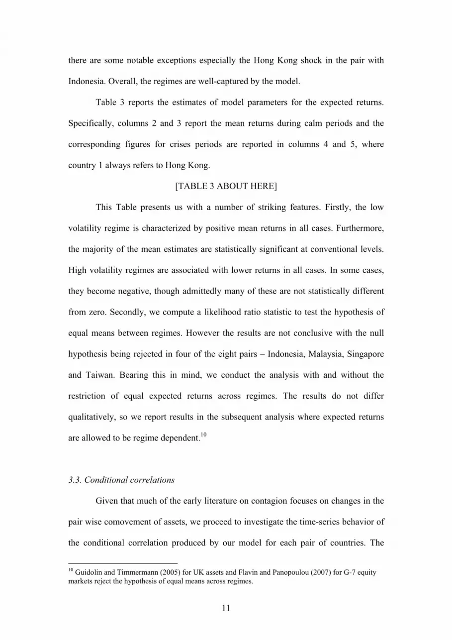
3.3. Conditional correlations

Given that much of the early literature on contagion focuses on changes in the

pair wise comovement of assets, we proceed to investigate the time-series behavior of

the conditional correlation produced by our model for each pair of countries. The

10 Guidolin and Timmermann (2005) for UK assets and Flavin and Panopoulou (2007) for G-7 equity markets reject the hypothesis of equal means across regimes.

12

evolution of this conditional correlation (conditional on the prevailing state) over time

can be calculated by utilizing the estimated filter probabilities for each type of shock

(those for the common shock are depicted in Figure 2, with corresponding numbers

for the idiosyncratic shocks in Figs 3 and 4) and the implied conditional covariance

matrix of returns (Eqs 6 and 7 show these covariance matrices for the extreme states).

The filter probabilities give the probability of being in each state for each shock given

the history of the process up to that point of time. Figure 1 provides a graphical

illustration of the conditional correlation for each pair of markets.

[FIGURE 1 ABOUT HERE]

The most striking feature is the amount of time variation exhibited by all market pairs.

This finding is consistent with Longin and Solnik (1995) and Karolyi and Stulz

(1996) among others. Bordo and Murshid (2000) show that over a period of 108

years, stock market correlations have exhibited large variation, both in tranquil and

crisis periods. It is clear from visual inspection that the correlation coefficients exhibit

considerable time variation. For many markets, most notably Korea and Thailand,

there is a large increase in the coefficient around the time of the Asian crisis but high

correlations are by no means exclusive to this time period. Contrary to expectations,

the correlation of Hong Kong/Malaysia appears to decline during the crisis period.

This finding is consistent with Dungey et al. (2006), who show that the sign of the

correlation change can be ambiguous. We can also observe a pattern similar to that

documented by Chiang et al. (2007), whereby there is a gradual increase in the

correlation in the first phase of the crisis and then a sustained second phase, which

they surmise to be driven by herding behavior in the market. However, it is clear that

one cannot conclude that contagion has taken place or not without performing formal

statistical tests for its presence.

13

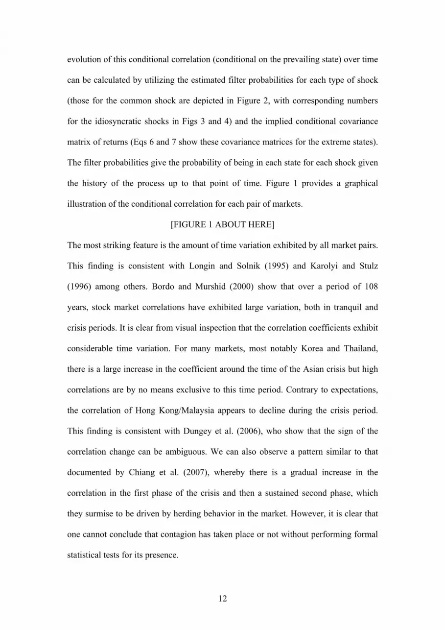
3.4. Tests for shift contagion

Initially we focus on shift contagion. Following GKM (2006), our test for shift

contagion focuses on changes in the transmission mechanism of common shocks

between low- and high-volatility regimes for pairs of markets. Therefore, we begin

our investigation with an in-depth analysis of this type of shock

[FIGURE 2 ABOUT HERE]

Figure 2 presents us with the filtered probabilities of the common shock being

in the high-volatility regime for each pair of markets. We observe a similar pattern

across most market pairs, with the common shock often being in the turbulent regime

and this is most evident around the Asian crisis from 1997-1998. In fact, in many

cases the turbulent regime is seen to persist for much longer and continued into the

start of the next decade. The early part of the 1990s is also characterized by high-

volatility common shocks and is consistent with events documented in Ito and

Hashimoto (2005).

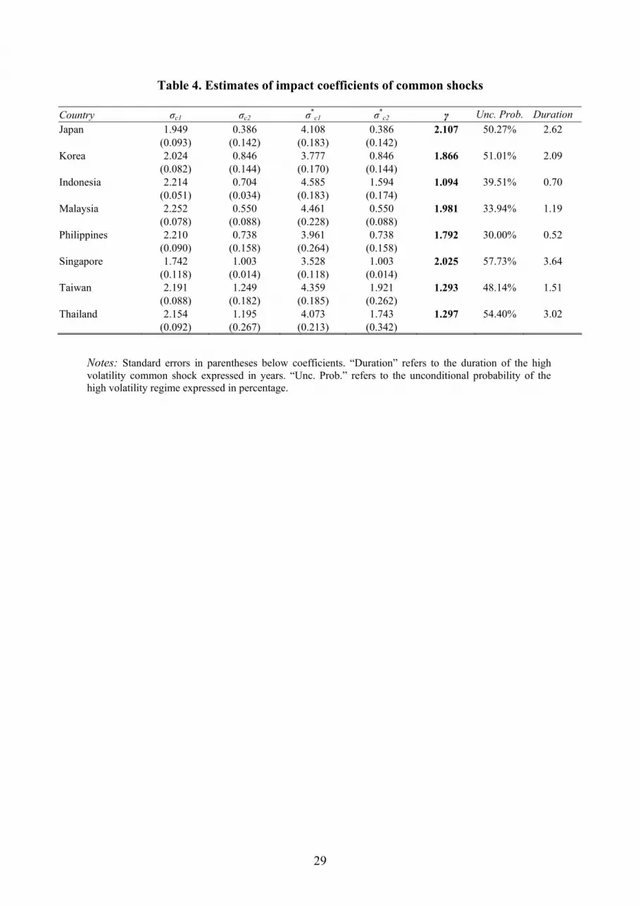
[TABLE 4 ABOUT HERE]

Table 4 presents a more detailed description of our results pertaining to the

characteristics of the common shock. Firstly, the column labeled ‘Unc Prob’ tells us

the proportion of time the common shock of each pair is in the high volatility state. It

is calculated as (1-P)/(2-P-Q), where P and Q are as defined in Eq. 4. It varies from a

high of 58% in the case of the Singapore/Hong Kong pair to a low of 30% for the

Philippines/Hong Kong pair. Therefore, it is clear that all pairs involving Hong Kong

are prone to common shocks that are quite often in a state of high-volatility.

Averaging over all market pairs, we see that the common shock is in the turbulent

14

regime approximately 45% of the time. Therefore, we have ample observations in this

regime with which to precisely estimate parameters.

The column labeled ‘Duration’ gives the length of time (in years) for which a

common shock persists – Duration = 1/(1-P). Common shock duration ranges from

six months for the Philippines/ Hong Kong pair to over 3.5 years for Singapore/Hong

Kong. These pairs also have the lowest and highest statistics for being in the high-

volatility regime respectively. The average duration across pairs is almost two years.

This shows that Hong Kong and all other markets were vulnerable to quite persistent,

high-volatility common shocks over the entire sample. It is clear from Figure 1 that,

for most pairs, this long persistence of the common shock is being driven by regional

and global market conditions from 1997 – 2001. All markets suffer common high-

volatility shocks arising from first the well-documented Asian crisis, which is regional

but the common shocks continue in the turbulent regime due to global events such as

the Russian crisis, the collapse of the LTCM hedge fund and the threat of global

terrorism following 9/11 in the US. Therefore it is important to recognize that to test

for shift contagion, common shocks do not have to be exclusively sourced in the

countries sampled.

The remainder of Table 4 presents our estimates of the impact coefficients of

common structural shocks for calm (σ) and turbulent (σ*) times (columns 2-3 and 4-5

respectively) as well as the ratio, γ, (column 6) which allows us to test for shift

contagion. Focusing on the structural impact coefficients, we find that the coefficients

in the low-volatility state are generally lower and with less dispersion that their

counterparts in the more turbulent regime. The calm regime has an average response

of 1.46 across all market pairs as opposed to 2.61 in the high-volatility state. Likewise

the average dispersion across parameters increases twofold. However, all estimated

15

parameters are statistically significantly different from zero. Furthermore, it is

instructive to distinguish between the structural impacts of Hong Kong and each of

the other countries recorded in response to a common shock. In both regimes, Hong

Kong is much more sensitive to these shocks but particularly in the high-volatility

regime. Often, we see that the response of the second country to entering a high-

volatility regime is largely unchanged but for Hong Kong, there is always an increase

in the estimated coefficient. Therefore, without any formal test, we can surmise that

this is likely to result in shift contagion.

To formulate a test for shift contagion, we report the ratio of the estimated

impact coefficients of common structural shocks in column 6 of Table 4. We

construct the following statistic:

.,max2

*1

1*2

1*2

2*1

=cc

cc

cc

cc

σσσσ

σσσσ

γ

This reveals whether impact coefficients in the high volatility regime are proportional

to their corresponding values in the low volatility regime. A ratio of unity indicates

that there is no difference in the transmission mechanism of shocks between the high-

and low-volatility regimes, whereas deviations from unity would imply market

contagion.

Given the aforementioned difference in common shock sensitivities observed

between Hong Kong and the other markets, it is unsurprising to find that this ratio is

always greater than unity and substantially so in many cases. To test whether or not it

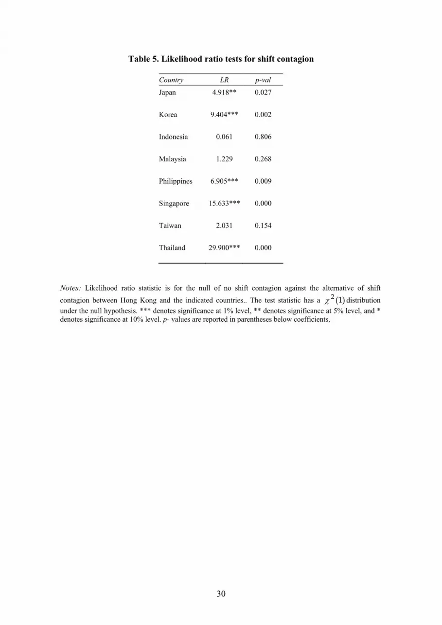
is statistically different from unity, we perform a likelihood ratio test, whose test

statistic has a )1(2χ distribution under the null hypothesis. Table 5 presents the

results.

[TABLE 5 ABOUT HERE]

16

We find strong evidence in favor of shift contagion in five markets – Japan,

Korea, the Philippines, Singapore and Thailand. When the common shocks between

these markets and Hong Kong enters the high-volatility regime, they experience a

structural shift in their interdependencies and hence, the diffusion of such shocks is

regime dependent. Evidence of shift contagion is observed for both developed

markets like Japan and emerging markets such as Thailand. In this respect, our results

are consistent with others who find that contagious effects can be experienced in

developed as well as developing markets (see Dungey et al., 2006). It is important to

note that in all cases, except Thailand, the change in the transmission mechanism

governing common shocks is being driven by the response of Hong Kong to the shock

entering the high-volatility regime. For the other countries - Japan, Korea, the

Philippines and Singapore – there is no additional response to the change in regime.

However, the Hong Kong response is sufficient to generate shift contagion. The

change in the structural parameter of country 2 to the common shock entering the

high-volatility regime seems to depend on the coincidence of the high-volatility

regime of the three shocks. For example, let’s contrast Japan and Thailand.

Comparing Figures 2 and 3, we observe that when the common shock of Hong / Japan

is in the high-volatility regime, the idiosyncratic shock of Hong Kong is also usually

in the high-volatility regime. Given that it is our source country, its idiosyncratic

shock impacts on the Japanese equity return during periods of market turbulence in

the former market. Therefore it appears that when the high-volatility regimes are

roughly coincident (for the common and idiosyncratic shock, the proportion of time

spent in this regime is 50% and 48% respectively), then the idiosyncratic shocks

impacting on Japanese equity swamp the effect of the common shock, leaving its

response unchanged between regimes. On the other hand, the common shock for

17

Thailand is far more often in the turbulent state than the idiosyncratic shock of Hong-

Kong for this pair (54% versus 12%). Hence the high-volatility regime for the

common shock exerts additional influence on the Thai equity return relative to its

normal level, causing the structural parameter to increase.

The presence of shift contagion has important implications for both investors

and policymakers. Investors will be reluctant to simultaneously hold equities in Hong

Kong and each of these markets because market linkages are not robust to changes in

market conditions. Policymakers who want to implement appropriate strategy to limit

the spread of contagion will have to look at measures to strengthen existing linkages

and reduce vulnerability to common shocks. On the other hand, there is no evidence

of shift contagion for Hong Kong and the markets of Indonesia, Malaysia and Taiwan.

The degree of interdependence observed in normal market conditions continues to

prevail in turbulent periods. Investors and policymakers should not be concerned by

the fear of changes to the normal levels of co-movement.

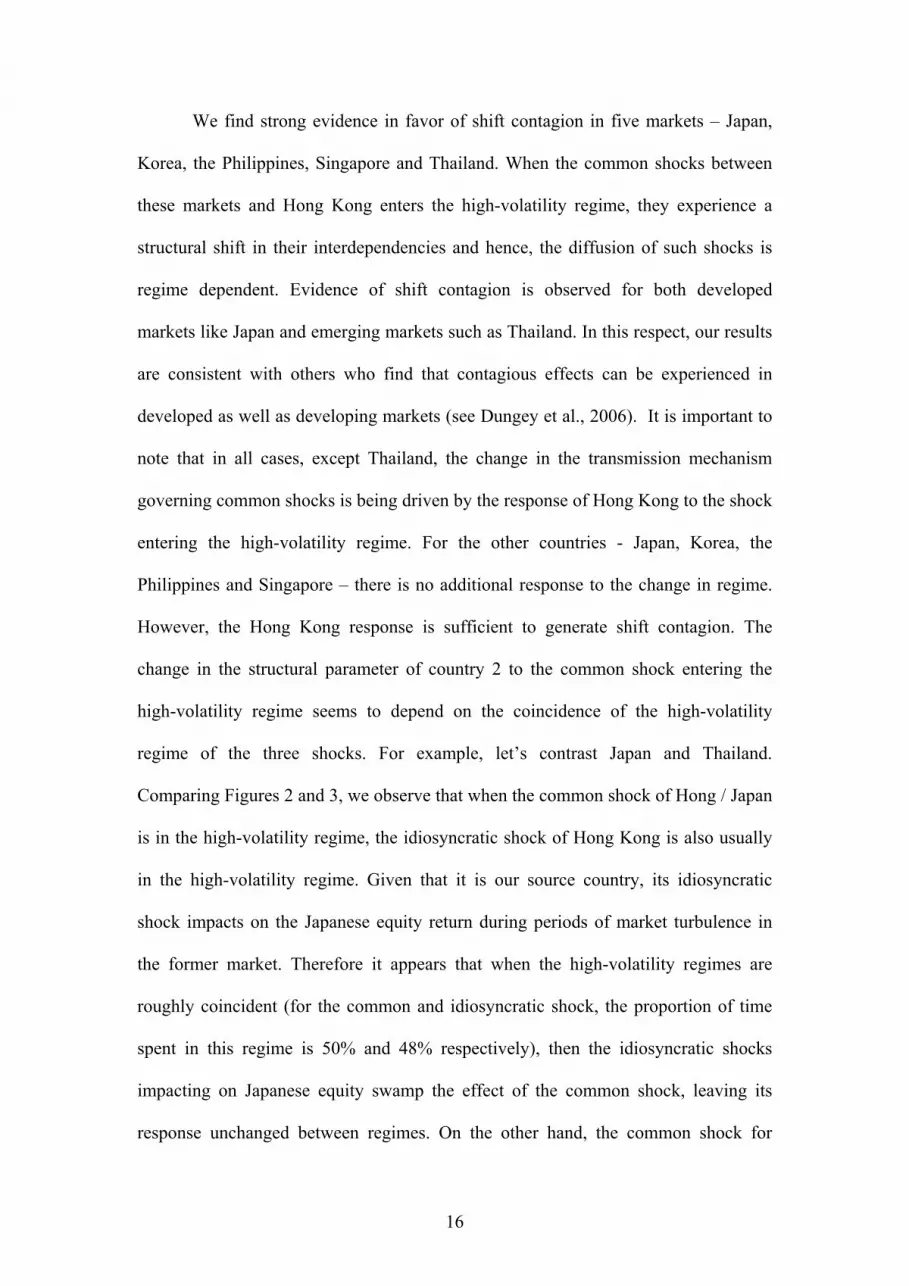
3.5. Tests for pure contagion

Pure contagion refers to the phenomenon whereby the idiosyncratic shock of

one country (Hong Kong in our case) is transmitted to others through channels that

only exist during periods of market turbulence. We now focus on the idiosyncratic

shocks and statistical tests of pure contagion.

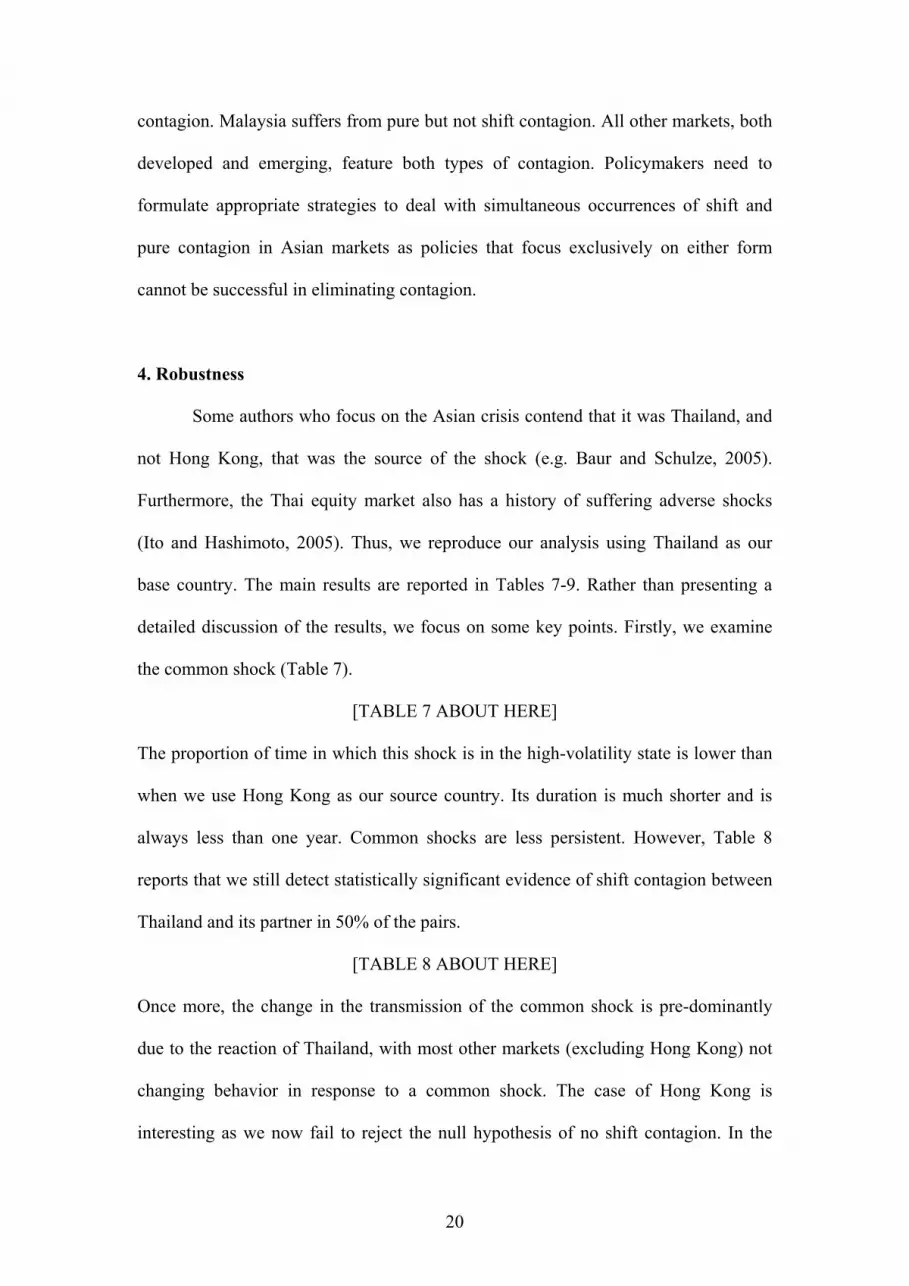
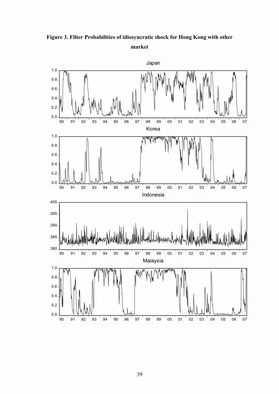
[FIGURES 3 & 4 ABOUT HERE]

Figure 3 presents the filtered probabilities of Hong Kong’s idiosyncratic shock being

in the turbulent regime, while Figure 4 depicts the equivalent information for each of

the other markets. In each of these bivariate analyses, we observe a great deal of

idiosyncratic risk associated with the Hong Kong market – the only exception being

18

with Indonesia. In all other cases, there is a large probability of being in the high-

volatility state, especially during the period of regional and global downturns. This is

very evident from 1997 onwards, which lends support to Hong Kong being the shock

source for the Asian crisis. Figure 4 focuses on the other market in the pair and

portrays a less consistent pattern. Some countries like Korea and Malaysia have

relatively few periods when the probability of being in the high-volatility regime is

close to one. On the other hand, others such as Japan, Singapore and Thailand have

many periods when their idiosyncratic shock is likely to experience high-volatility. As

stated above, turbulent conditions for the Hong Kong shock often coincide with

similar conditions for the common shock.

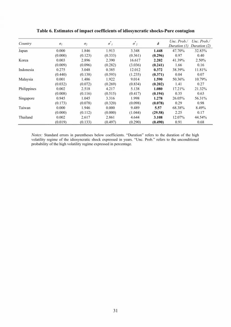
[TABLE 6 ABOUT HERE]

Table 6 gives a more in-depth analysis of results pertaining to these

idiosyncratic shocks. There is much more variation in the structural impact

coefficients compared to the common shock and all exhibit huge variation between

regimes. All countries record a significant increase in sensitivity to switches between

regimes for these shocks. Column 7 gives information on the proportion of time that

the Hong Kong shock spends in the high-volatility regime and its duration, while

column 8 contains the corresponding statistics for the other markets in the bivariate

analysis. For Hong Kong, the time spent in the turbulent state varies from a low of

12% for the pair with Thailand to a high of 68% for the Taiwanese pair. The shock

duration is short relative to that of its common counterpart. For the pair with

Indonesia, it persists for only a couple of weeks but at the other end of the spectrum, it

persists for over two years in the pair with Taiwan. For all pairs, there is sufficient

variation to suspect that the Hong Kong idiosyncratic shock might instigate pure

contagion. In the case of the other markets, there is large variation in the prevalence of

19

the diversifiable shock and its duration is generally short – less than one year in all

instances.

Column 6 of Table 6 reports the estimated coefficients (with standard errors)

for the δ parameter, which detects and measures the strength of pure contagion. The

high-volatility country-specific shock of Hong Kong has adverse repercussions for its

neighboring markets and exerts a strong influence on their return generating process.

The δ parameter is positive for all countries and statistically different from zero in six

out of eight cases. With the exception of Indonesia and Taiwan, we find evidence that

the idiosyncratic shock of Hong Kong was transmitted to each of the other markets in

our analysis. These pure contagion effects were felt most strongly in the developing

markets of Thailand and Korea. However even developed markets like Japan also

suffered from pure contagious effects from Hong Kong. Combining the results in

Tables 4 and 6, the transmission of high-volatility idiosyncratic shocks from Hong

Kong to adjacent markets causes the greatest impact on equity returns for its

neighbors, while its own response to turbulent common shocks is more pronounced.

Consequently we find evidence of both contagion types.

3.6. Summary of results

Combining the results of the previous two sections, we can conclude that our

sample of the past 17 years is characterized by significant contagion from Hong Kong

to many of its neighboring East Asian equity markets. We find statistically significant

evidence of both shift and pure contagion being present in the majority of markets.

Only Taiwan and Indonesia appear to be immune from contagious effects, with no

evidence of either type of contagion. Interestingly, Bekaert et al. (2005) finds that

Taiwan is the only Asian country in their sample which does not experience

20

contagion. Malaysia suffers from pure but not shift contagion. All other markets, both

developed and emerging, feature both types of contagion. Policymakers need to

formulate appropriate strategies to deal with simultaneous occurrences of shift and

pure contagion in Asian markets as policies that focus exclusively on either form

cannot be successful in eliminating contagion.

4. Robustness

Some authors who focus on the Asian crisis contend that it was Thailand, and

not Hong Kong, that was the source of the shock (e.g. Baur and Schulze, 2005).

Furthermore, the Thai equity market also has a history of suffering adverse shocks

(Ito and Hashimoto, 2005). Thus, we reproduce our analysis using Thailand as our

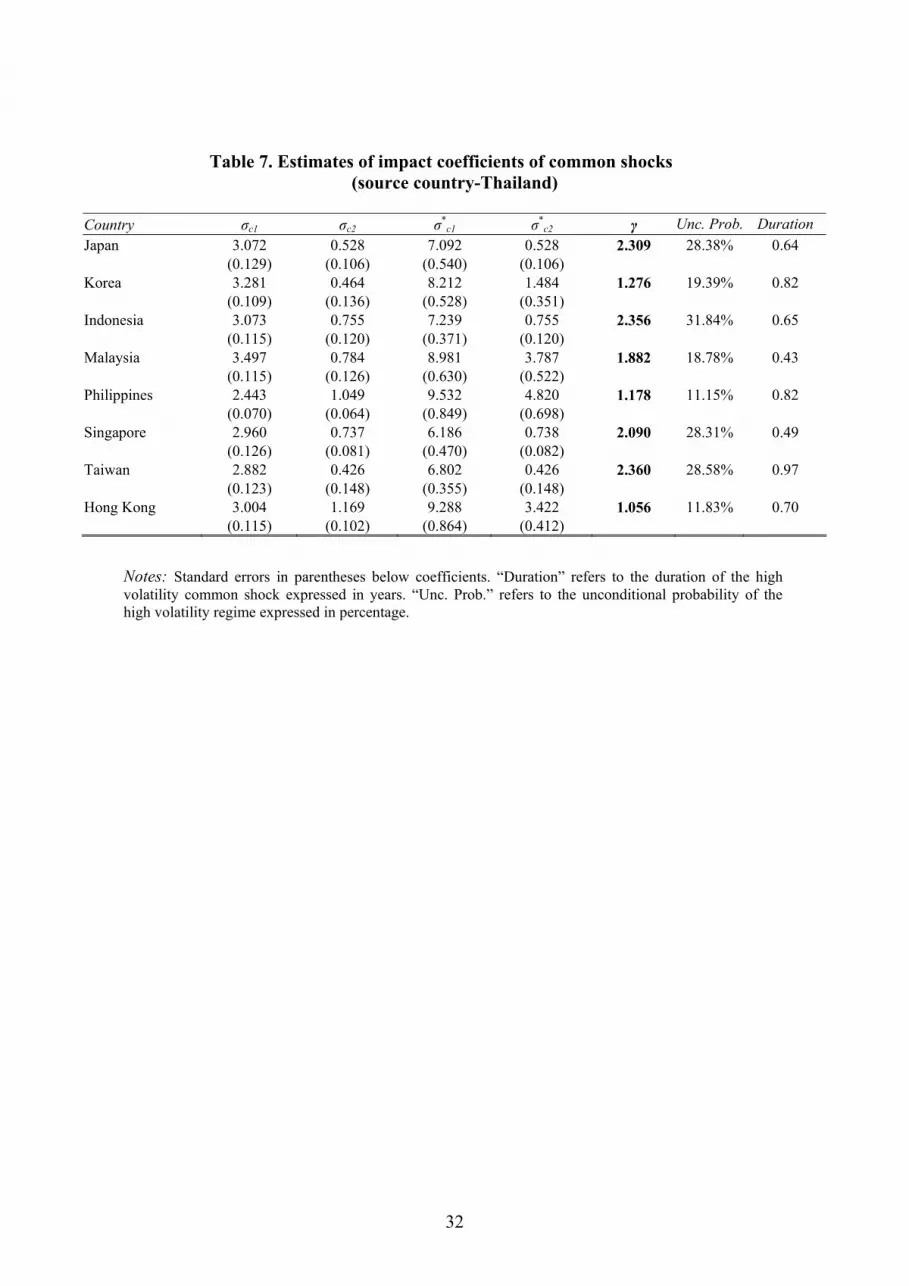
base country. The main results are reported in Tables 7-9. Rather than presenting a

detailed discussion of the results, we focus on some key points. Firstly, we examine

the common shock (Table 7).

[TABLE 7 ABOUT HERE]

The proportion of time in which this shock is in the high-volatility state is lower than

when we use Hong Kong as our source country. Its duration is much shorter and is

always less than one year. Common shocks are less persistent. However, Table 8

reports that we still detect statistically significant evidence of shift contagion between

Thailand and its partner in 50% of the pairs.

[TABLE 8 ABOUT HERE]

Once more, the change in the transmission of the common shock is pre-dominantly

due to the reaction of Thailand, with most other markets (excluding Hong Kong) not

changing behavior in response to a common shock. The case of Hong Kong is

interesting as we now fail to reject the null hypothesis of no shift contagion. In the

21

previous section, this was reversed as the influence of the Hong Kong idiosyncratic

shock outweighed the response of Thai equity returns to the high-volatility common

shock, suggesting that shift contagion had taken place. However, when the source

country is specified as Thailand, its idiosyncratic shock does not impact upon Hong

Kong (see below) and therefore all the increased equity volatility comes through the

common shock. This result shows that the importance of selecting the proper source

country.

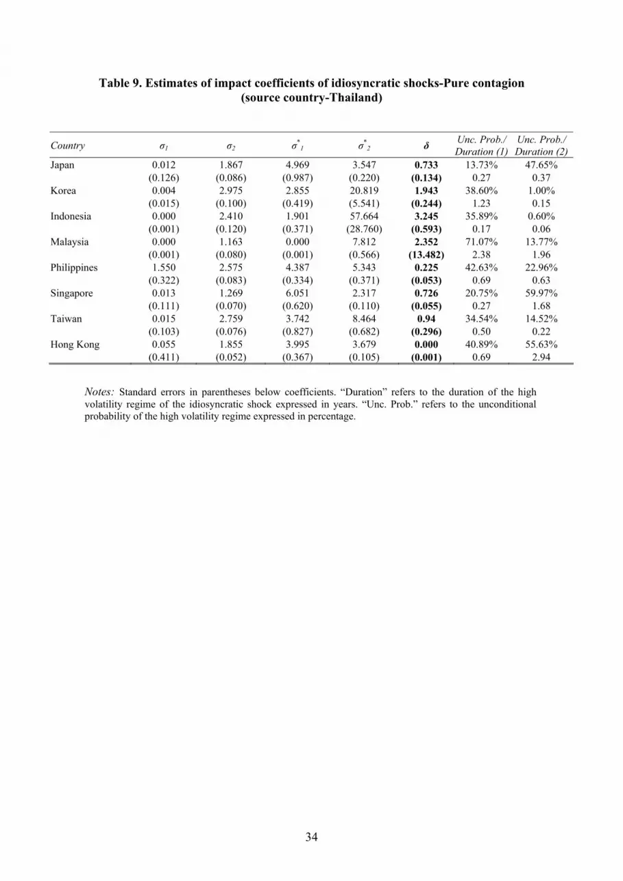
Results pertaining to the idiosyncratic shocks and tests of pure contagion are

reported in Table 9.

[TABLE 9 ABOUT HERE]

The prevalence and persistence of the idiosyncratic shocks show great variation across

market pairs. In contrast to the previous case, the idiosyncratic shocks display far

greater persistence than the common shock. This may be due to more factors between

other markets and Hong Kong rather than Thailand. The idiosyncratic shock of Hong

Kong again exhibits slow decay. Once more, there is evidence of pure contagion

effects running from Thailand to many other markets. In particular, Indonesia and

Korea are vulnerable to such contagion for its Thai neighbor. Indonesia which was

immune to contagious effects from Hong Kong is severely exposed to Thai shocks,

consistent with the findings of Cerra and Saxena (2002). Only Malaysia and Hong

Kong appear to be unaffected by the high-volatility of the Thai idiosyncratic shock.

Therefore Hong Kong is unaffected by Thailand but the reverse is not true.

Whether we use, Hong Kong or Thailand as our shock source, we find

considerable evidence of both shift and pure contagion within the region. Focusing on

the Hong Kong – Thailand pairs that are common, it suggests that Thailand is

sensitive to Hong Kong volatility but not the reverse. Indonesia, on the other hand, is

22

susceptible to contagious effects from Thailand but not Hong Kong. Both developed

and emerging markets are vulnerable to this phenomenon.

5. Conclusions

We set about testing for both shift and pure contagion effects within a unified

framework. Our methodology is a factor model, often used in financial economics,

and extends the model of GKM (2006). We have a bivariate model in which the

unexpected element of equity returns are decomposed into a common shock and an

idiosyncratic component. Both constituent shocks are allowed to switch between

volatility regimes, yielding a model in which returns may transit between four (eight)

states. We base our tests on the equity markets of East Asia. This model appears to

capture return behavior quite well.

We use both Hong Kong and Thailand as base countries and test for both

changes in the transmission of common shocks between pairs of markets (shift

contagion) and also for influences of idiosyncratic shocks from the base country on

other neighboring markets. Using Hong Kong as our shock source, there is statistical

evidence for the presence of both types of contagion in five markets. Most often, the

instances of shift contagion result from the response of Hong Kong to high-volatility

in the common shock. Malaysia suffers pure contagious effects but no change in the

diffusion process governing the common shock. Only Indonesia and Thailand appear

to be completely immune to contagion from Hong Kong. Employing Thailand as our

base country reinforces the conclusion that contagion has been a major feature of East

Asian equity markets over the past two decades.

Our results have major implications for both investors and policymakers.

Investors should be cautious about simultaneously holding equities from two

23

countries which exhibit shift contagion. The promised portfolio benefits are likely to

disappear when most needed, given that the transmission of common shocks change

during periods with high-volatility common shocks. Policymakers charged with

formulating strategy to curb the spread of contagion across the region should take

account of the fact that there appears to be two distinct types of contagion operating at

the same time. Policies designed to exclusively treat one form of contagion without

due regard for the other are likely to be unsuccessful.

Acknowledgments

We would like to thank participants at the International Equity Markets Comovements

and Contagion conference, Cass City Business School (May 2007) and the 1st MIFN

workshop (Maastricht, September 2007) for helpful comments and suggestions on an

earlier version of the paper. We would also like to thank James Morley for making the

Gauss code for testing shift contagion available to us. Panopoulou thanks the Irish

Higher Education Authority for providing research support under the North South

Programme for Collaborative Research. The usual disclaimer applies.

24

References

Ang, A., Bekaert, G., 2002. International asset allocation with regime shifts. Review of Financial studies, 15, 1137-1187.

Baur, D., Schulze, N., 2005. Co-exceedances in financial markets: a quantile regression analysis of contagion. Emerging Markets Review, 6, 21-43.

Bekaert, G., Harvey, C., Ng, A., 2005. Market integration and contagion. Journal of Business, 78(1), 39-69.

Billio, M., Pelizzon, L., 2003. Contagion and interdependence in stock markets: have they been misdiagnosed? Journal of Economics and Business, 55, 405-426.

Bond, S., Dungey, M., Fry, R., 2006. A web of shocks: crises across Asian real estate markets. Journal of Real Estate Finance and Economics, 32(3), 253-274.

Bordo, M.D., Murshid, A.P., 2000. Are financial crises becoming increasingly more contagious? What is the historical evidence on contagion? NBER paper no. 7900.

Caporale, G., Cipollini, A., Spagnolo, N., 2003. Testing for contagion: a conditional correlation analysis. Journal of Empirical Finance, 12, 476-489.

Cerra, V., Saxena, S.C., 2002. Contagion, monsoons and domestic turmoil in Indonesia’s currency crisis. Review of International Economics, 10, 36-44.

Chiang, T.C., Jeon, B.N., Li, H., 2007. Dynamic correlation analysis of financial contagion: evidence from Asian markets. Journal of International Money and Finance, 26, 1206-1228.

Dungey, M., Fry, R., Gonzalez-Hermosillo, B., Martin, V.L., (2005). Empirical modeling of contagion: a review of methodologies. Quantitative Finance, 5, 9-24. Dungey, M., Fry, R., Gonzalez-Hermosillo, B., Martin, V.L., (2007). Sampling properties of contagion tests. Unpublished manuscript, University of Cambridge. Dungey, M., Fry, R., Martin, V., 2003. Equity transmission mechanisms from Asia to Australia: interdependence or contagion? Australian Journal of Management, 28(2), 157-182. Dungey, M., Fry, R., Martin, V., 2004. Currency market contagion in the Asia-Pacific region. Australian Economic Papers, 43(4), 379-395. Dungey, M., Fry, R., Martin, V., 2006. Correlation, contagion and Asian evidence. Asian Economic Journal, forthcoming. Dungey, M., Tambakis, D.N., 2005. International financial contagion: what should we be looking for? In Dungey, M., Tambakis, D.M. (Eds) Identifying International Financial Contagion: Progress and Challenges, Oxford University Press, NY.

25

Flavin, T., Panopoulou, E, 2007. On the robustness of international portfolio diversification benefits to regime-switching volatility. Journal of International Financial Markets, Institutions and Money, forthcoming. Forbes, K.J., Rigobon, R.J., 2002. No contagion, only interdependence: measuring stock market comovements. Journal of Finance, 57 (5), 2223-61. Goetzmann, W., Li, L., Rouwenhorst, K.G., 2002. Long-term global market correlations. Working Paper no. 8612, National Bureau of Economic Research, Cambridge, MA. Gravelle, T., Kichian, M., Morley, J., 2006. Detecting shift-contagion in currency and bond markets. Journal of International Economics, 68 (2), 409-423.

Guidolin, M., Timmermann, A., 2005. Economic implications of bull and bear regimes in UK stock and bond returns, Economic Journal, 115, 111-143. Hamilton, J.D., 1989. A new approach to the economic analysis of nonstationary time series and the business cycle, Econometrica, 57, 357-384.

Ito, T., Hashimoto, Y., 2005. High-frequency contagion between exchange rates and stock prices during the Asian currency crisis. In Dungey, M., Tambakis, D.M. (Eds) Identifying International Financial Contagion: Progress and Challenges, Oxford University Press, NY.

Karolyi, G.A., 2003. Does international financial contagion really exist? International Finance, 6(2), 179-199.

Karolyi, G. A., Stulz, R. M., 1996. Why Do Markets Move Together? An Investigation of U.S. – Japan Stock Return Co-movements, Journal of Finance, 51, 951–86. Longin, F., Solnik, B., 1995. Is the correlation in international equity returns constant: 1960 – 1990? Journal of International Money and Finance, 14, 3-26. Pericoli, M., Sbracia, M., 2003. A primer on financial contagion. Journal of Economic Surveys, 17(4), 571-608. Rigobon, R., 2003a. Identification through heteroskedasticity. The Review of Economics and Statistics, 85(4), 777-792.

Rigobon, R., 2003b. On the measurement of the international propagation of shocks: is the transmission stable? Journal of International Economics, 61(2), 261-283.

26

Table 1.

Panel A. Summary Descriptive Statistics

Japan Korea Indonesia Malaysia Philippines Singapore Taiwan Thailand Hong Kong

Mean 0.063 0.248 0.257 0.185 0.169 0.165 0.094 0.189 0.292 Median 0.000 0.176 0.071 0.275 0.213 0.161 0.145 0.099 0.441 Maximum 12.50 30.73 70.92 36.24 17.34 16.96 29.42 26.47 15.12 Minimum -12.14 -44.13 -41.52 -32.28 -25.46 -20.34 -21.98 -24.11 -18.25 Std. Dev. 3.139 5.129 5.244 4.057 3.965 2.887 4.710 4.999 3.337 Skewness 0.375 -0.053 2.410 0.344 -0.218 -0.285 0.507 0.298 -0.247 Kurtosis 4.526 13.957 44.614 22.657 7.316 8.553 8.011 6.684 5.922

Jarque Bera 109.5 (0.000)

4547.8 (0.000)

66469.7 (0.000)

14652.6 (0.000)

712.8 (0.000)

1180.4 (0.000)

990.1 (0.000)

527.4 (0.000)

332.5 (0.000)

Panel B. Correlation

Market Japan Korea Indonesia Malaysia Philippines Singapore Taiwan Thailand Hong Kong

Japan 1.000 0.322 0.197 0.256 0.216 0.419 0.279 0.286 0.331 Korea 1.000 0.265 0.275 0.293 0.442 0.267 0.428 0.406 Indonesia 1.00 0.262 0.341 0.325 0.163 0.313 0.258 Malaysia 1.00 0.399 0.507 0.262 0.417 0.381 Philippines 1.000 0.502 0.308 0.467 0.414 Singapore 1.000 0.401 0.583 0.636 Taiwan 1.000 0.307 0.377 Thailand 1.000 0.439 Hong Kong 1.000

27

Table 2. Diagnostic tests on standardized residuals and model specification

Country LM(1) LM(4) ARCH(1) ARCH(4) Normality RCM1 RCM2 RCM3 Japan 0.853 4.419 0.294 3.881 0.056 54.58 60.49 23.38 2.823 6.184 3.677 7.024 0.078 Korea 0.319 3.914 0.145 5.008 0.029 24.47 3.47 30.06 0.036 7.839 7.220* 10.526 0.042 Indonesia 0.734 4.084 0.001 8.132 0.063 94.51 20.26 32.64 0.406 15.467* 54.107* 7.054 0.191* Malaysia 0.173 2.903 0.494 8.112 0.061 33.10 11.67 27.03 5.936 11.880 2.462 24.203* 0.041 Philippines 0.239 1.329 0.026 0.627 0.124 25.01 28.97 39.58 3.637 12.794 0.046 2.019 0.029 Singapore 0.155 5.741 0.099 5.561 0.038 32.71 53.13 22.89 0.809 11.784 15.259* 82.430* 0.144 Taiwan 0.824 3.961 0.224 8.367 0.046 34.38 13.97 31.17 0.000 8.378 0.602 9.256 0.085 Thailand 0.158 2.287 0.540 1.476 0.025 11.38 55.77 25.04 0.515 11.587 25.872* 45.360* 0.067

Notes: LM(k) is the Breusch-Godfrey Lagrange Multiplier test for no serial correlation up to lag k,

ARCH(k) is the Lagrange Multiplier test for no ARCH effects of order k, Normality is the Cramer-von-

Mises test for the null of Normality, RCMi is the Regime Classification Measure, where i=1,2,3 for the

idiosyncratic shock of the first, second and the common shock, respectively. * denotes significance at

1% level. LM(k) and ARCH(k) have a )(2 kχ distribution under the null hypothesis. The Cramer-von-

Mises test has a non-standard distribution and the cut-off value for RCM is 50.

28

Table 3. Estimates of mean returns across regimes

Country µ1 µ2 µ*1 µ*

2 LR p-val Japan 0.410 0.080 0.161 -0.002 1.010 0.603 (0.109) (0.167) (0.207) (0.020) Korea 0.481 0.246 0.097 0.180 2.939 0.230 (0.102) (0.169) (0.143) (0.204) Indonesia 0.469 0.646 -0.003 -0.673 4.857* 0.088 (0.102) (0.153) (0.025) (0.236) Malaysia 0.412 0.329 0.034 -0.106 5.597* 0.061 (0.105) (0.092) (0.052) (0.179) Philippines 0.563 0.662 -0.311 -1.035 4.595 0.101 (0.108) (0.144) (0.441) (0.315) Singapore 0.509 0.479 0.175 0.115 4.756* 0.093 (0.104) (0.102) (0.048) (0.096) Taiwan 0.466 0.293 0.072 -0.205 14.573*** 0.001 (0.111) (0.177) (0.135) (0.344) Thailand 0.447 0.301 0.163 0.284 1.628 0.443 (0.101) (0.136) (0.152) (0.122)

Notes: Standard errors in parentheses below coefficients. Likelihood ratio statistic is for the null of equality of mean returns across the regimes. The test statistic has a )2(2χ distribution under the null hypothesis. *** denotes significance at 1% level, ** denotes significance at 5% level, and * denotes significance at 10% level.

29

Table 4. Estimates of impact coefficients of common shocks

Country σc1 σc2 σ*c1 σ*

c2 γ Unc. Prob. Duration Japan 1.949 0.386 4.108 0.386 2.107 50.27% 2.62 (0.093) (0.142) (0.183) (0.142) Korea 2.024 0.846 3.777 0.846 1.866 51.01% 2.09 (0.082) (0.144) (0.170) (0.144) Indonesia 2.214 0.704 4.585 1.594 1.094 39.51% 0.70 (0.051) (0.034) (0.183) (0.174) Malaysia 2.252 0.550 4.461 0.550 1.981 33.94% 1.19 (0.078) (0.088) (0.228) (0.088) Philippines 2.210 0.738 3.961 0.738 1.792 30.00% 0.52 (0.090) (0.158) (0.264) (0.158) Singapore 1.742 1.003 3.528 1.003 2.025 57.73% 3.64 (0.118) (0.014) (0.118) (0.014) Taiwan 2.191 1.249 4.359 1.921 1.293 48.14% 1.51 (0.088) (0.182) (0.185) (0.262) Thailand 2.154 1.195 4.073 1.743 1.297 54.40% 3.02 (0.092) (0.267) (0.213) (0.342)

Notes: Standard errors in parentheses below coefficients. “Duration” refers to the duration of the high volatility common shock expressed in years. “Unc. Prob.” refers to the unconditional probability of the high volatility regime expressed in percentage.

30

Table 5. Likelihood ratio tests for shift contagion

Country LR p-val

Japan 4.918** 0.027 Korea 9.404*** 0.002 Indonesia 0.061 0.806 Malaysia 1.229 0.268 Philippines 6.905*** 0.009 Singapore 15.633*** 0.000 Taiwan 2.031 0.154 Thailand 29.900*** 0.000

Notes: Likelihood ratio statistic is for the null of no shift contagion against the alternative of shift

contagion between Hong Kong and the indicated countries.. The test statistic has a )1(2χ distribution under the null hypothesis. *** denotes significance at 1% level, ** denotes significance at 5% level, and * denotes significance at 10% level. p- values are reported in parentheses below coefficients.

31

Table 6. Estimates of impact coefficients of idiosyncratic shocks-Pure contagion

Country σ1 σ2 σ*1 σ*

2 δ Unc. Prob./ Duration (1)

Unc. Prob./ Duration (2)

Japan 0.000 1.846 1.913 3.348 1.448 47.70% 32.83% (0.000) (0.123) (0.333) (0.361) (0.296) 0.97 0.40 Korea 0.003 2.896 2.390 16.617 2.202 41.39% 2.50% (0.009) (0.096) (0.282) (3.036) (0.241) 1.66 0.16 Indonesia 0.275 3.048 0.385 12.012 0.372 38.39% 11.81% (0.440) (0.138) (0.593) (1.235) (0.371) 0.04 0.07 Malaysia 0.001 1.486 1.922 9.014 1.590 50.36% 10.79% (0.032) (0.072) (0.269) (0.834) (0.202) 1.41 0.27 Philippines 0.002 2.518 4.217 5.138 1.080 17.21% 21.32% (0.008) (0.116) (0.515) (0.417) (0.194) 0.35 0.63 Singapore 0.945 1.045 3.316 1.998 1.278 26.05% 56.31% (0.173) (0.078) (0.320) (0.098) (0.078) 0.29 0.98 Taiwan 0.000 1.946 0.000 9.489 5.57 68.38% 8.49% (0.000) (0.112) (0.000) (1.044) (29.58) 2.25 0.17 Thailand 0.002 2.617 2.861 4.644 3.108 12.07% 44.54% (0.019) (0.133) (0.497) (0.290) (0.490) 0.91 0.68

Notes: Standard errors in parentheses below coefficients. “Duration” refers to the duration of the high volatility regime of the idiosyncratic shock expressed in years. “Unc. Prob.” refers to the unconditional probability of the high volatility regime expressed in percentage.

32

Table 7. Estimates of impact coefficients of common shocks (source country-Thailand)

Country σc1 σc2 σ*

c1 σ*c2 γ Unc. Prob. Duration

Japan 3.072 0.528 7.092 0.528 2.309 28.38% 0.64 (0.129) (0.106) (0.540) (0.106) Korea 3.281 0.464 8.212 1.484 1.276 19.39% 0.82 (0.109) (0.136) (0.528) (0.351) Indonesia 3.073 0.755 7.239 0.755 2.356 31.84% 0.65 (0.115) (0.120) (0.371) (0.120) Malaysia 3.497 0.784 8.981 3.787 1.882 18.78% 0.43 (0.115) (0.126) (0.630) (0.522) Philippines 2.443 1.049 9.532 4.820 1.178 11.15% 0.82 (0.070) (0.064) (0.849) (0.698) Singapore 2.960 0.737 6.186 0.738 2.090 28.31% 0.49 (0.126) (0.081) (0.470) (0.082) Taiwan 2.882 0.426 6.802 0.426 2.360 28.58% 0.97 (0.123) (0.148) (0.355) (0.148) Hong Kong 3.004 1.169 9.288 3.422 1.056 11.83% 0.70 (0.115) (0.102) (0.864) (0.412)

Notes: Standard errors in parentheses below coefficients. “Duration” refers to the duration of the high volatility common shock expressed in years. “Unc. Prob.” refers to the unconditional probability of the high volatility regime expressed in percentage.

33

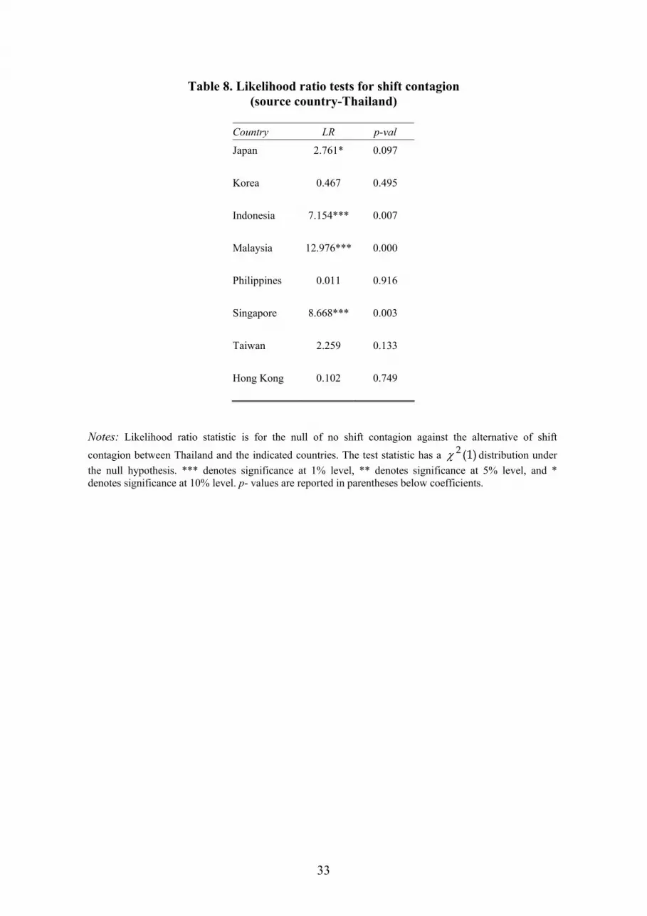
Table 8. Likelihood ratio tests for shift contagion (source country-Thailand)

Country LR p-val

Japan 2.761* 0.097 Korea 0.467 0.495 Indonesia 7.154*** 0.007 Malaysia 12.976*** 0.000 Philippines 0.011 0.916 Singapore 8.668*** 0.003 Taiwan 2.259 0.133 Hong Kong 0.102 0.749

Notes: Likelihood ratio statistic is for the null of no shift contagion against the alternative of shift

contagion between Thailand and the indicated countries. The test statistic has a )1(2χ distribution under the null hypothesis. *** denotes significance at 1% level, ** denotes significance at 5% level, and * denotes significance at 10% level. p- values are reported in parentheses below coefficients.

34

Table 9. Estimates of impact coefficients of idiosyncratic shocks-Pure contagion (source country-Thailand)

Country σ1 σ2 σ*1 σ*

2 δ Unc. Prob./ Duration (1)

Unc. Prob./ Duration (2)

Japan 0.012 1.867 4.969 3.547 0.733 13.73% 47.65% (0.126) (0.086) (0.987) (0.220) (0.134) 0.27 0.37 Korea 0.004 2.975 2.855 20.819 1.943 38.60% 1.00% (0.015) (0.100) (0.419) (5.541) (0.244) 1.23 0.15 Indonesia 0.000 2.410 1.901 57.664 3.245 35.89% 0.60% (0.001) (0.120) (0.371) (28.760) (0.593) 0.17 0.06 Malaysia 0.000 1.163 0.000 7.812 2.352 71.07% 13.77% (0.001) (0.080) (0.001) (0.566) (13.482) 2.38 1.96 Philippines 1.550 2.575 4.387 5.343 0.225 42.63% 22.96% (0.322) (0.083) (0.334) (0.371) (0.053) 0.69 0.63 Singapore 0.013 1.269 6.051 2.317 0.726 20.75% 59.97% (0.111) (0.070) (0.620) (0.110) (0.055) 0.27 1.68 Taiwan 0.015 2.759 3.742 8.464 0.94 34.54% 14.52% (0.103) (0.076) (0.827) (0.682) (0.296) 0.50 0.22 Hong Kong 0.055 1.855 3.995 3.679 0.000 40.89% 55.63% (0.411) (0.052) (0.367) (0.105) (0.001) 0.69 2.94

Notes: Standard errors in parentheses below coefficients. “Duration” refers to the duration of the high volatility regime of the idiosyncratic shock expressed in years. “Unc. Prob.” refers to the unconditional probability of the high volatility regime expressed in percentage.

35

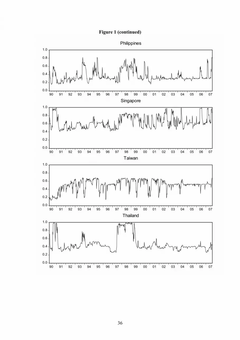
Figure 1. Conditional Correlations

0.0

0.2

0.4

0.6

0.8

1.0

90 91 92 93 94 95 96 97 98 99 00 01 02 03 04 05 06 07

Japan

0.0

0.2

0.4

0.6

0.8

1.0

90 91 92 93 94 95 96 97 98 99 00 01 02 03 04 05 06 07

Korea

0.0

0.2

0.4

0.6

0.8

1.0

90 91 92 93 94 95 96 97 98 99 00 01 02 03 04 05 06 07

Indonesia

0.0

0.2

0.4

0.6

0.8

1.0

90 91 92 93 94 95 96 97 98 99 00 01 02 03 04 05 06 07

Malaysia

36

Figure 1 (continued)

0.0

0.2

0.4

0.6

0.8

1.0

90 91 92 93 94 95 96 97 98 99 00 01 02 03 04 05 06 07

Philippines

0.0

0.2

0.4

0.6

0.8

1.0

90 91 92 93 94 95 96 97 98 99 00 01 02 03 04 05 06 07

Singapore

0.0

0.2

0.4

0.6

0.8

1.0

90 91 92 93 94 95 96 97 98 99 00 01 02 03 04 05 06 07

Taiwan

0.0

0.2

0.4

0.6

0.8

1.0

90 91 92 93 94 95 96 97 98 99 00 01 02 03 04 05 06 07

Thailand

37

Figure 2. Filter Probabilities of high volatility common shocks

0.0

0.2

0.4

0.6

0.8

1.0

90 91 92 93 94 95 96 97 98 99 00 01 02 03 04 05 06 07

Japan

0.0

0.2

0.4

0.6

0.8

1.0

90 91 92 93 94 95 96 97 98 99 00 01 02 03 04 05 06 07

Korea

0.0

0.2

0.4

0.6

0.8

1.0

90 91 92 93 94 95 96 97 98 99 00 01 02 03 04 05 06 07

Indonesia

0.0

0.2

0.4

0.6

0.8

1.0

90 91 92 93 94 95 96 97 98 99 00 01 02 03 04 05 06 07

Malaysia

38

Figure 2 (continued)

0.0

0.2

0.4

0.6

0.8

1.0

90 91 92 93 94 95 96 97 98 99 00 01 02 03 04 05 06 07

Philippines

0.0

0.2

0.4

0.6

0.8

1.0

90 91 92 93 94 95 96 97 98 99 00 01 02 03 04 05 06 07

Singapore

0.0

0.2

0.4

0.6

0.8

1.0

90 91 92 93 94 95 96 97 98 99 00 01 02 03 04 05 06 07

Taiwan

0.0

0.2

0.4

0.6

0.8

1.0

90 91 92 93 94 95 96 97 98 99 00 01 02 03 04 05 06 07

Thailand

39

Figure 3. Filter Probabilities of idiosyncratic shock for Hong Kong with other

market

0.0

0.2

0.4

0.6

0.8

1.0

90 91 92 93 94 95 96 97 98 99 00 01 02 03 04 05 06 07

Japan

0.0

0.2

0.4

0.6

0.8

1.0

90 91 92 93 94 95 96 97 98 99 00 01 02 03 04 05 06 07

Korea

.380

.385

.390

.395

.400

90 91 92 93 94 95 96 97 98 99 00 01 02 03 04 05 06 07

Indonesia

0.0

0.2

0.4

0.6

0.8

1.0

90 91 92 93 94 95 96 97 98 99 00 01 02 03 04 05 06 07

Malaysia

40

Figure 3 (continued)

0.0

0.2

0.4

0.6

0.8

1.0

90 91 92 93 94 95 96 97 98 99 00 01 02 03 04 05 06 07

Philippines

0.0

0.2

0.4

0.6

0.8

1.0

90 91 92 93 94 95 96 97 98 99 00 01 02 03 04 05 06 07

Singapore

0.0

0.2

0.4

0.6

0.8

1.0

90 91 92 93 94 95 96 97 98 99 00 01 02 03 04 05 06 07

Taiwan

0.0

0.2

0.4

0.6

0.8

1.0

90 91 92 93 94 95 96 97 98 99 00 01 02 03 04 05 06 07

Thailand

41

Figure 4. Filter Probabilities of country idiosyncratic shock

0.0

0.2

0.4

0.6

0.8

1.0

90 91 92 93 94 95 96 97 98 99 00 01 02 03 04 05 06 07

Japan

0.0

0.2

0.4

0.6

0.8

1.0

90 91 92 93 94 95 96 97 98 99 00 01 02 03 04 05 06 07

Korea

0.0

0.2

0.4

0.6

0.8

1.0

90 91 92 93 94 95 96 97 98 99 00 01 02 03 04 05 06 07

Indonesia

0.0

0.2

0.4

0.6

0.8

1.0

90 91 92 93 94 95 96 97 98 99 00 01 02 03 04 05 06 07

Malaysia

42

Figure 4 (continued)

0.0

0.2

0.4

0.6

0.8

1.0

90 91 92 93 94 95 96 97 98 99 00 01 02 03 04 05 06 07

Philippines

0.0

0.2

0.4

0.6

0.8

1.0

90 91 92 93 94 95 96 97 98 99 00 01 02 03 04 05 06 07

Singapore

0.0

0.2

0.4

0.6

0.8

1.0

90 91 92 93 94 95 96 97 98 99 00 01 02 03 04 05 06 07

Taiwan

0.0

0.2

0.4

0.6

0.8

1.0

90 91 92 93 94 95 96 97 98 99 00 01 02 03 04 05 06 07

Thailand

Institute for International Integration StudiesThe Sutherland Centre, Trinity College Dublin, Dublin 2, Ireland