Detecting Ecosystem Reliance on Groundwater Based on Satellite-Derived Greenness Anomalies and Temporal Dynamics

283

13Detecting Ecosystem Reliance on Groundwater Based on Satellite-Derived Greenness Anomalies and Temporal Dynamics

S. ContrerasCentre of Pedology and Applied Biology of Segura, Spain

D. Alcaraz-SeguraUniversity of Granada, Spain; University of Almería, Spain

B. ScanlonThe University of Texas at Austin, Texas

E. G. JobbágySan Luis Institute of Applied Mathematics (IMASL), Argentina

CONTENTS

13.1 Introduction ................................................................................................28413.2 Methods ....................................................................................................... 286

13.2.1 Study Site ......................................................................................... 28613.2.2 Climate and Satellite Dataset for Greenness Anomaly

Estimation .......................................................................................28813.2.3 Greenness Timing and Metrics.................................................... 29013.2.4 Impact of Groundwater on Vegetation Dynamics:

A Conceptual Model ..................................................................... 29113.3 Results and Discussion ............................................................................. 292

13.3.1 MAP-EVI Regional Function ........................................................ 29213.3.2 EVI Dynamics along a Groundwater Dependence

Gradient at the Telteca Site ........................................................... 292

284 Earth Observation of Ecosystem Services

13.1 Introduction

Groundwater-dependent ecosystems (GDEs) play a key role in human development, and are especially relevant in regions with low rates of rain-fall, by providing a broad range of ecosystem services such as physical sup-port for wildlife habitats and biodiversity hotspots, control of floods and erosion, regulation of nutrient cycling, or provision of landscape refuges for cognitive development (de Groot et al. 2002; Chen et al. 2004; Eamus et al. 2005; Bergkamp and Katharine 2006; Ridolfi et al. 2007). During the past decade, research on ecology and functioning of GDEs has received a grow-ing interest from the scientific community and from landscape managers. However, in spite of their high intrinsic values, many of these ecosystems have been strongly impacted as a consequence of disruption of hydrological linkages with groundwater resources. This disruption has been generally promoted by excessive rates of groundwater extraction and depletion, for example, Las Tablas de Daimiel and Doñana National Reserves in Spain (Llamas 1988; Muñoz-Reinoso and García-Novo 2005); Swan Coastal Plain in southwest Australia (Groom et al. 2000); desert springs in the Mojave and Great Basin deserts in the United States (Patten et al. 2008); San Pedro River in the United States (Stromberg et al. 1996). It has also been caused by modi-fication of morphology of stream channels or wetlands through dredging or artificial diversions (Ellery and McCarthy 1998) or as a consequence of changes in their water balance due to climatic factors (Murray-Hudson et al. 2006). A better understanding of the functioning and water consumption of GDEs is then critically required to evaluate the ecological services pro-vided by them (Murray et al. 2006; Brauman et al. 2007) and, for develop-ing adaptive management frameworks that reconcile compatible human activities, ecosystem conservation, and their underlying hydrological trade-offs under future scenarios of land use and climate change (MacKay 2006; Barron et al. 2012b).

GDEs are ecosystems that require groundwater inflows to maintain their current structure and functioning and the subsequent delivery of eco-system services (Hatton and Evans 1997; Murray et al. 2003; Eamus et al. 2006). GDEs may display an obligate reliance requiring a constant ground-water presence, or a facultative one where they adapt their functioning to fluctuating groundwater availability (Murray et al. 2003; Bertrand

13.3.3 Intercomparison among Phreatophytic Woodlands, Wetlands, and Irrigated Crops ..................................................... 295

13.4 Conclusions ................................................................................................. 298Acknowledgments .............................................................................................. 299References ............................................................................................................. 299

Dow

nloa

ded

by [

Serg

io C

ontr

eras

] at

10:

01 0

7 Ja

nuar

y 20

14

285Phenometrics in Groundwater Dependent Ecosystems

et al. 2012). According to the aquifer–ecosystem interface relationship, GDEs include (Eamus et al. 2006; Eamus 2009): (a) caves and subterranean-aquatic ecosystems, including karst aquifers and rock-fractured systems; (b) ecosystems dependent on permanent or temporary surface expres-sions of groundwater, including baseflow riverine, spring, wetland or peatland, and estuarine/marine-shoreline ecosystems; and (c) ecosystems dependent on the subsurface presence of groundwater, also termed “ter-restrial GDEs” or phreatophytic ecosystems (Richardson et al. 2011). Other pedological, morphological, hydrological, and biogeochemical criteria have been proposed for classifying GDEs from a functional point of view (Bertrand et al. 2012).

To preserve their ecological integrity and service provision, GDEs require water allocation plans and adaptive management strategies rooted in knowl-edge about their (a) typology and spatial distribution, (b) quantitative water requirements, and (c) resistance and resilience to natural and human per-turbations on their groundwater regimes. A wide range of methodological approaches and techniques are commonly employed to accomplish these three aspects, including remote sensing, water balance analysis, hydro-geological modeling, tracer and isotopic studies, ecophysiological mea-surements, rooting system characterization, and aquatic fauna sampling (see Richardson et al. 2011 for a synthesis).

Tracking photosynthetic/greenness activity of vegetation using satellite-based indices such as Normalized Difference Vegetation Index (NDVI) or Enhanced Vegetation Index (EVI) offers a relatively inexpensive and effec-tive way to characterize the functioning of riparian/wetland and terrestrial GDEs (Bradley and Mustard 2008; Barron et al. 2012a). These spectral indi-ces are well correlated with aboveground net primary productivity (ANPP) and evapotranspiration (ET) in semiarid regions (Running and Nemani 1988; Paruelo et al. 1997; Jobbágy et al. 2002; Nagler et al. 2005; Guerschman et al. 2009) (see Chapter 18). When they are not influenced by the presence of groundwater and lateral-inflow resources, annual rates of ANPP and ET in those regions are primarily controlled by precipitation and, second, by radiation forcing and its seasonal coupling with rainfall inputs (Specht 1972; Specht and Specht 1989; Ellis and Hatton 2008; Palmer et al. 2010). Because groundwater supplies a more temporally reliable water source for terrestrial ecosystems than rainfall, higher and more stable ET and ANPP rates should be expected in GDEs compared to their nongroundwater ecosystem counter-parts (Contreras et al. 2011; O’Grady et al. 2011). Field observations show that leaf area, ANPP, and water availability are closely correlated, supporting the use of satellite-based vegetation indices for the identification and character-ization of GDEs, including the quantification of their water requirements at different temporal scales (Nagler et al. 2005; Contreras et al. 2011; Devitt et al. 2011; O’Grady et al. 2011). Field evidence also suggests that even when access to unlimited groundwater resources exists, the productivity of GDEs could be strongly constrained by other limiting resources or processes such

Dow

nloa

ded

by [

Serg

io C

ontr

eras

] at

10:

01 0

7 Ja

nuar

y 20

14


as incoming energy, nutrient availability, morphological constraints, or dis-turbances, among others (Eamus et al. 2000; Do et al. 2008). Consequently, it seems that annual primary productivity estimates retrieved from annual summaries of spectral vegetation indexes could not be sufficient to identify and characterize the water requirements of terrestrial GDEs. To solve this potential constraint, complementary assessment of seasonal greenness timing can provide additional and valuable information on the functional response of ecosystems to their environment (Morisette et al. 2009). In these studies, in addition to primary productivity estimates, seasonality and phenology traits are commonly retrieved from annual greenness dynam-ics of ecosystems to classify and characterize ecosystem functional types, that is, patches of land surface with similar exchanges of matter and energy between the biota and the physical environment (Paruelo et al. 2001; Alcaraz-Segura et al. 2006; Fernández et al. 2010) (see Chapters 9 and 16).

This study aims to evaluate a satellite-based approach for identifying inflow-dependent ecosystems and to detect the type and degree of ground-water reliance of wetland and phreatophytic ecosystems. The approach con-sists of the complementary analysis of the annual greenness anomalies computed according to Contreras et al. (2011), and land surface phenological metrics retrieved from intra-annual and interannual greenness trajectories. The performance of this approach is tested in the lowlands of the central Monte Desert (Argentina), where a potential gradient of native inflow- dependent ecosystems has been previously identified. Finally, productivity, seasonality, and phenological metrics computed for a representative sam-ple of those types of ecosystems are compared with those extracted from a sample of sites located at an upstream irrigated oasis that exploits surface and groundwater resources for its maintenance.

13.2 Methods

13.2.1 Study Site

The study region covers an area of 87,500 km2 of lowlands (≤ 1000 m a.s.l.) and expands over the central Monte Desert in Argentina between 31° S and 36° S (Figure 13.1). The region is bounded by the Andes Cordillera to the west and by the Sierras Pampeanas to the east. Precipitation in the region ranges from 150 to 400 mm y−1, most of it concentrated in the austral summer (from October to March), and mean annual temperature ranges from 13°C to 19°C. Potential evapotranspiration reaches 1400 mm y−1 in the driest parts of the study region. A detailed review of the main biophysical and socioeconomic characteristics of the Monte Desert is provided by Abraham et al. (2009), while Villagra et al. (2009) review some of the effects that land use and disturbance factors have had on the dynamics of the natural ecosystems of this desert.

Dow

nloa

ded

by [

Serg

io C

ontr

eras

] at

10:

01 0

7 Ja

nuar

y 20

14


The area is crossed by five major rivers (from north to south: San Juan, Mendoza, Tunuyán, Diamante, and Atuel) with their origins in the Andes Cordillera. After crossing the mountains, these rivers reach the alluvial fans and sedimentary plains of the central Monte Desert to finally discharge into the Desaguadero-Salado river system. Andean rivers are the main sources of water for four large artificial oases located in the foothills of the region (Figure 13.1), with vineyards, olives, and fruit trees being the main crops. These oases represent approximately 90% of the economic activity in the region, and more than 1.5 million people live there. Along their route in the alluvial funs, rivers recharge large unconsolidated aquifers that extend downstream of the artificial oases to reach the lowlands of the region that are covered by sandy plains of fluvial, lacustrine, and eolian origin.

Alluvial and lowland plains at the foothills of the Andes are mainly covered by three types of ecosystems: (a) shrub-steppes dominated by Larrea spp. (jarillales), (b) open phreatophytic woodlands of Prosopis spp. trees (locally known as algarrobales), and (c) marshes and wetlands that are along the main rivers. Two of the largest wetland systems are the Rosario system—at the last section of the Mendoza River just before its confluence with the

BA <–0.1<0.00

0.15

>+0.1>0.30

0.0A, a

C

FIGURE 13.1 (See color insert.)Study region and mean annual values of EVI (A, left) and EVI anomalies (B, right) computed from September 2000 through August 2009. Main rivers in lowercase letters: (a) San Juan River; (b) Mendoza River; (c) Tunuyán River; (d) Diamante River; (e) Atuel River; and (f) Desaguadero-Salado River. Irrigated oases in capital letters: (A) San Juan oasis; (B) Mendoza oasis; (C) Upper Tunuyan oasis; and (D) San Rafael oasis. Sample sites in control areas (black squares) were located at the open Prosopis woodlands of the Telteca Natural Reserve and surroundings (T_wood), the Rosario and Guanacache wetland systems (R_wet and G_wet, respectively) and irrigated crops at the Mendoza oasis (MIO_agr).

Dow

nloa

ded

by [

Serg

io C

ontr

eras

] at

10:

01 0

7 Ja

nuar

y 20

14


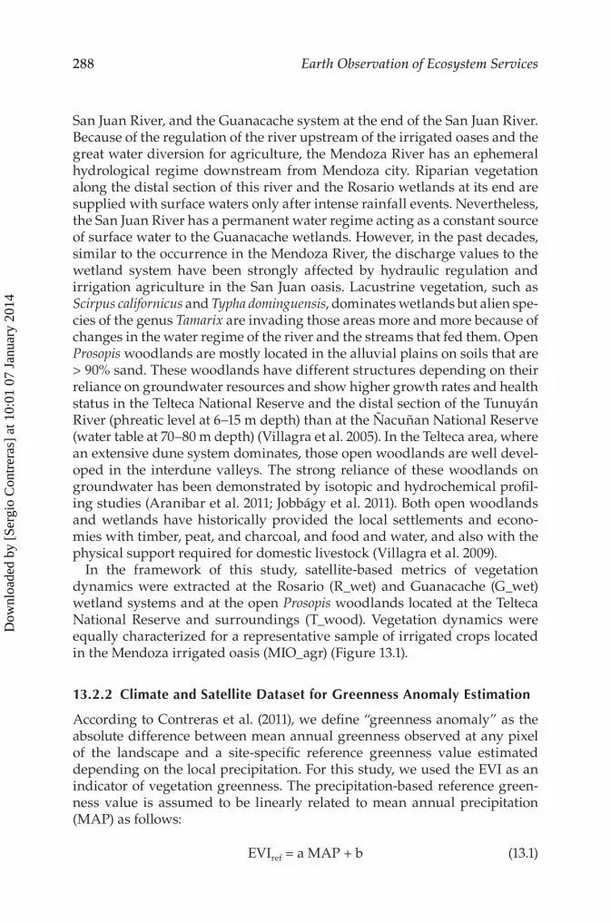
San Juan River, and the Guanacache system at the end of the San Juan River. Because of the regulation of the river upstream of the irrigated oases and the great water diversion for agriculture, the Mendoza River has an ephemeral hydrological regime downstream from Mendoza city. Riparian vegetation along the distal section of this river and the Rosario wetlands at its end are supplied with surface waters only after intense rainfall events. Nevertheless, the San Juan River has a permanent water regime acting as a constant source of surface water to the Guanacache wetlands. However, in the past decades, similar to the occurrence in the Mendoza River, the discharge values to the wetland system have been strongly affected by hydraulic regulation and irrigation agriculture in the San Juan oasis. Lacustrine vegetation, such as Scirpus californicus and Typha dominguensis, dominates wetlands but alien spe-cies of the genus Tamarix are invading those areas more and more because of changes in the water regime of the river and the streams that fed them. Open Prosopis woodlands are mostly located in the alluvial plains on soils that are > 90% sand. These woodlands have different structures depending on their reliance on groundwater resources and show higher growth rates and health status in the Telteca National Reserve and the distal section of the Tunuyán River (phreatic level at 6–15 m depth) than at the Ñacuñan National Reserve (water table at 70–80 m depth) (Villagra et al. 2005). In the Telteca area, where an extensive dune system dominates, those open woodlands are well devel-oped in the interdune valleys. The strong reliance of these woodlands on groundwater has been demonstrated by isotopic and hydrochemical profil-ing studies (Aranibar et al. 2011; Jobbágy et al. 2011). Both open woodlands and wetlands have historically provided the local settlements and econo-mies with timber, peat, and charcoal, and food and water, and also with the physical support required for domestic livestock (Villagra et al. 2009).

In the framework of this study, satellite-based metrics of vegetation dynamics were extracted at the Rosario (R_wet) and Guanacache (G_wet) wetland systems and at the open Prosopis woodlands located at the Telteca National Reserve and surroundings (T_wood). Vegetation dynamics were equally characterized for a representative sample of irrigated crops located in the Mendoza irrigated oasis (MIO_agr) (Figure 13.1).

13.2.2 Climate and Satellite Dataset for Greenness Anomaly Estimation

According to Contreras et al. (2011), we define “greenness anomaly” as the absolute difference between mean annual greenness observed at any pixel of the landscape and a site-specific reference greenness value estimated depending on the local precipitation. For this study, we used the EVI as an indicator of vegetation greenness. The precipitation-based reference green-ness value is assumed to be linearly related to mean annual precipitation (MAP) as follows:

EVIref = a MAP + b (13.1)

Dow

nloa

ded

by [

Serg

io C

ontr

eras

] at

10:

01 0

7 Ja

nuar

y 20

14


where EVIref is precipitation-based EVI and a and b are fitted-parameters computed empirically from a quantile regression analysis developed over the observed EVI-MAP scatterplot defined for a set of reference sites. We assumed a linear relationship between EVI and evapotranspiration based on the field data support available for semiarid regions (e.g., Nagler et al. 2005; Guerschman et al. 2009; O’Grady et al. 2011). With such assumption, we are able to estimate the expected EVI value for a vegetation cover that exclusively uses local precipitation and is in equilibrium with long-term precipitation (Boer and Puigdefábregas 2003; Contreras et al. 2008). This condition, in which annual ET approaches the MAP, has been proposed to be reached at our study region for 75th quantile threshold value (Contreras et al. 2011). At an annual timescale, we defined the concept of EVI anomaly as follows:

EVIa = EVIma − EVImap (13.2)

where EVIma is the observed annual average of EVI computed from satel-lite images at each pixel, and EVImap is the EVIref in Equation 13.1 estimated using the 75th quantile threshold value. From a functional point of view, both metrics, EVIa and EVIma, are considered here as surrogates of primary productivity.

A map of MAP for the region, which is required to estimate EVImap, was calculated from long-term average monthly values reported in the CRU CL 2.0 dataset (New et al. 2002), which were previously corrected with data from the CLIMWAT 2.0 database (FAO 2006) and local meteorological stations. Maps of precipitation were finally resampled to a 250-m spatial resolution, which is compatible with the satellite data (Contreras et al. 2011).

The EVI MOD13Q1 land product from MODIS Collection 5 (Solano et al. 2010) was extracted for the region (tile h12v12) covering nine hydrological years from September 2001 through August 2009 (23 scenes per hydrologi-cal year). Before processing, raw EVI data at 250-m spatial resolution were filtered using a local polynomial function based on an adaptive Savitzky–Golay filter using the TIMESAT software (Jönsson and Eklundh 2004). EVI, which combines data from the blue, red, and infrared spectral bands, was preferable to NDVI because atmospheric interferences and soil background signal are more effectively removed and because of its greater sensitivity to high biomass situations (Huete et al. 2002).

Equation 13.1 was parameterized across 125 reference sites that meet the criteria of having low disturbance rates and lacking artificial or runoff water supplies (Contreras et al. 2008, 2011). From the resulting EVI-MAP scatterplot, three quantile threshold values were used here to propose a pre-liminary gradient of classes of groundwater reliance. First, as stated earlier, we used the 75th quantile regression of mean annual EVI versus MAP func-tion as a conservative value to generate EVImap values. Observed EVI values lower than EVImap (i.e., negative greenness anomaly values) were assumed

Dow

nloa

ded

by [

Serg

io C

ontr

eras

] at

10:

01 0

7 Ja

nuar

y 20

14


not to have any dependency on groundwater resources. For values higher than EVImap, a gradient of three potential classes of low, moderate, and high degree of reliance were established using the 75th, 90th, and 99th quantile thresholds, respectively. In this study, the former quantile threshold val-ues were arbitrarily selected in order to evaluate the potential agreement between the resulting reliance levels and the phenological metrics extracted from the greenness timing analysis.

13.2.3 Greenness Timing and Metrics

A representative sample of pixels for the four study systems (Telteca woodlands, Rosario and Guanacache wetlands, and irrigated crops at the Mendoza oasis) was selected for retrieving metrics, or phenomet-rics, related to vegetation traits of primary productivity, seasonality, and phenology (Figure 13.2). At the Telteca Reserve, 78 pixels were sampled to cover all the potential groundwater-reliance degrees identified by the anomaly greenness (no reliance, low, moderate, and high) although pixels

EVInrange=EVIrange/EVIma

EVI EVIma

EVImap

Tmin Tgs0 Tmax Tgs1

Lgseason

iEVIgseason

iEVIagseason

EVIrange

EVImax iEVIannual

EVImin

Time

EVIa

FIGURE 13.2Vegetation metrics retrieved from Enhanced Vegetation Index (EVI) trajectories to identify groundwater-dependent ecosystems and to quantify their reliance on groundwater. All met-rics were retrieved from annual (September–August) and average long-term seasonal trajec-tories. Metrics are related to productivity traits: EVIma = mean annual EVI; EVIgs = mean EVI accumulated during the growing season; seasonality traits: EVImax and EVImin = maximum and minimum EVI values; EVIrange = annual amplitude of EVI (EVImax – EVImin), EVInrange = normal-ized annual amplitude (EVIrange/EVIma); and phenology traits: Tmax and Tmin = times at which maximum and minimum EVI values are reached; Tgs0 and Tgs1 = times at which growing season starts and ends, Lgseason = growing season length. Productivity traits are estimated from inte-grated values of greenness at the annual (iEVIannual) and growing season (iEVIgs) scales. EVImap is the reference EVI value expected according the local mean annual precipitation and is required to compute greenness anomalies at the annual (EVIama) and growing season (EVIags).

Dow

nloa

ded

by [

Serg

io C

ontr

eras

] at

10:

01 0

7 Ja

nuar

y 20

14


with moderate- and high-reliance degrees were finally grouped together to obtain a more robust comparison among classes. In the wetland systems, vegetation metrics were only extracted from pixels (Guanacache, n = 40; Rosario, n = 10) with a potential high degree of reliance on groundwa-ter. Metrics related to vegetation primary productivity, seasonality, and phenology were extracted at intra-annual and interannual timescales from the average seasonal trajectory resulting from September 2000 to August 2009 (intra-annual variability) and from the annual trajectories for the nine hydrological years covered by the study (interannual variability). In this study, we extracted the following EVI metrics related to traits of: (a) vegetation productivity: EVIma and EVIgs; (b) vegetation seasonality: EVImin, EVImax, and EVInrange; and (c) vegetation phenology: Lgs and Tmax (see Figure 13.2 for more details).

13.2.4 Impact of Groundwater on Vegetation Dynamics: A Conceptual Model

From a functional point of view, a water table close to the land surface is expected to impact intra-annual (seasonal) and interannual (multiyear) variability of the EVI dynamics in several ways. The following hypothesis guided our analyses (Table 13.1).

At the intra-annual scale, we hypothesize that MAP (EVIma), the cumu-lated productivity during the growing season (EVIgs), and maximum (EVImax) and minimum (EVImin) values of greenness are expected to increase

TABLE 13.1

Trends in Vegetation Traits

Vegetation Traits Greenness Metrics Intra-Annual Scale Interannual Variability

Productivity EVIma ↑ ↓EVIgs ↑ ↓

Seasonality EVImax ↑ ↓

EVImin ↑ ↓

EVInrange ↓ ↓

Phenology Lgs ↑ ↓

Tmax ↑ ↓

Note: Trends (arrows) measured by satellite-based metrics expected in terrestrial GDEs as groundwater reliance increases. Metrics are related to productivity traits: EVIma = mean annual EVI; EVIgs = mean EVI accumulated during the growing season; season-ality traits: EVImax and EVImin = maximum and minimum EVI values; EVIrange = annual amplitude of EVI (EVImax – EVImin), EVInrange = normalized annual amplitude (EVIrange/EVIma); and phenology traits: Tmax = time at which maximum value is reached.

Dow

nloa

ded

by [

Serg

io C

ontr

eras

] at

10:

01 0

7 Ja

nuar

y 20

14


with greater reliance of ecosystems on groundwater. Because shallow water tables represent a perennial source of water for ecosystems, we also hypoth-esize that vegetation with any reliance on groundwater would show less variable seasonal trajectories of productivity (EVInrange) as groundwater reli-ance increases. As a consequence of less variability in the greenness trajec-tory (less EVInrange), a longer period should be required to reach 50% of the total annual productivity, here defined as the growing season length (Lgs). At the interannual scale, we expect that variability of all vegetation metrics described for productivity, seasonality, and phenology traits should be lower in GDEs than in non-GDEs and should decrease as reliance on groundwater increases. The matrix of conceptual rules proposed here to evaluate ecosys-tem reliance on groundwater has been designed under the assumption that the access to groundwater by vegetation remained relatively constant with-out large changes in the water table depth. Then, changes in the water table depth or in the hydrological regime of those ecosystems are expected to be followed by modifications in their greenness dynamics and phenological patterns.

13.3 Results and Discussion

13.3.1 MAP-EVI Regional Function

According to the MAP-EVI function described for the region (Figure 13.3), positive EVI anomalies cover 26,000 km2 (~30% of the total area) with 36% distributed over the irrigated oases of the region (Table 13.2; Figure 13.1). High positive anomalies represent almost 24% of the total positive anoma-lies mapped on natural ecosystems/rangelands, but almost 95% of the total area at irrigated oases, which proves the important role that irrigation has on agricultural development in the region.

13.3.2 EVI Dynamics along a Groundwater Dependence Gradient at the Telteca Site

Almost synchronous intra-annual (Figure 13.4) and interannual (Figure 13.5) trajectories of EVI were found in Prosopis woodlands located at the Telteca natural reserve, with annual and growing season values higher than those observed at the control sites (sites with no positive greenness anomalies) as EVI anomalies increased (Figure 13.6a). Trends in productivity metrics were also confirmed for seasonality values with higher EVImax and EVImin val-ues, but lower seasonality variation (EVInrange), as EVI anomalies increased (Figure 13.6b). No significant trends were found, however, for phenological metrics, that is, growing season length (Lgs) and time at which maximum

Dow

nloa

ded

by [

Serg

io C

ontr

eras

] at

10:

01 0

7 Ja

nuar

y 20

14


Reference sites

75th quantile regression90th quantile regression

99th quantile regression

MIO_agr sites

MAP (mm)

500.0

0.1

0.2

0.3

EVI

0.4

0.5

100 150 200 250 300 350 400 450 500 550

FIGURE 13.3 (See color insert.)Mean Annual Precipitation–Enhanced Vegetation Index (MAP-EVI) quantile regression functions for the study region. Sample of pixels selected at each control area (brown symbols) are embraced by dashed lines. Functions were computed from MAP-EVI values measured at 125 reference sites (black-white circles). EVI thresholds corresponding to 75th, 90th, and 99th quantile regressions are used to classify systems into their low, moderate, and high reliance on water inputs besides local precipitation, respectively.

TABLE 13.2

Negative and Positive Enhanced Vegetation Index (EVI) Anomalies

Type of Land CoverNegative Anomaly

Positive Anomaly

TotalLow Moderate High Total

Natural ecosystems or rangelands

61.526 6.416 6.222 3.846 16.483 78.009

Irrigated oases 265 139 334 8.796 9.269 9.534Total 61.791 6.555 6.556 12.642 25.752 87.543

Note: Total area (in km2) with negative and positive EVI anomalies in the study region. Positive and negative anomalies were computed from EVImap values estimated from 75th quantile regression function. Positive anomalies, which represent por-tions of landscape with any reliance degree on water inputs besides precipitation, have been divided into low, moderate, and high levels of reliance if EVI is higher than 75th, 90th, and 99th quantile threshold values, respectively.

Dow

nloa

ded

by [

Serg

io C

ontr

eras

] at

10:

01 0

7 Ja

nuar

y 20

14


EVI is reached (Tmax), although average values for both were higher than control sites as EVI anomalies increased (Figure 13.6c). Because patterns and trends predicted by our conceptual model were matched at the Telteca woodlands, it seems that greenness anomaly may be a good surrogate for the reliance that woodland ecosystems have on groundwater resources. In addition to the metrics and trends recorded, a higher increase rate in the greenness trajectory was also observed during the late spring period, from November to December, in sites with moderately high EVI anomalies than in the control sites (Figure 13.4). This “early upraise” makes EVI differences among sites the highest during this seasonal period when energy constraints (low temperatures) start to disappear for phreatophytic woodlands, but rain-fall inputs are still low for promoting vegetation growth in their nonphreato-phytic counterparts.

Significant differences in EVI annual values were found throughout the entire study period between control sites and sites with moderately high EVI anomalies (Figure 13.5). Although weak absolute differences in EVI were observed, those differences were not significant between sites with

T_woodland (0) G_wetland (+++)R_wetland (+++)MIO_agr (+++)

T_woodland (+)T_woodland (++/+++)

–0.05

Sep

5

Oct

7

Nov

8

Dec

10

Jan

8

Feb

9

Mar

13

Apr

14

May

16

Jun

17

Jul 1

9

Aug

20

0.00

0.05

0.10

0.15

0.20

0.25

0.30

EVI an

om

FIGURE 13.4Mean seasonal Enhanced Vegetation Index (EVI) anomaly trajectories observed for represen-tative sites. Trajectories were extracted for groups of sample of pixels with different levels of reliance on water inputs besides local precipitation (0: no reliance; +: low reliance; ++: moderate reliance; +++: high reliance); T_woodland = open Prosopis woodlands at Telteca; G_wetland = Guanacache wetland; R_wetland = Rosario wetland; MIO_agr = Mendoza irrigated oasis (agroecosystem).

Dow

nloa

ded

by [

Serg

io C

ontr

eras

] at

10:

01 0

7 Ja

nuar

y 20

14


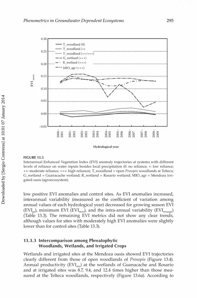
low positive EVI anomalies and control sites. As EVI anomalies increased, interannual variability (measured as the coefficient of variation among annual values of each hydrological year) decreased for growing season EVI (EVIgs), minimum EVI (EVImin), and the intra-annual variability (EVInrange) (Table 13.3). The remaining EVI metrics did not show any clear trends, although values for sites with moderately high EVI anomalies were slightly lower than for control sites (Table 13.3).

13.3.3 Intercomparison among Phreatophytic Woodlands, Wetlands, and Irrigated Crops

Wetlands and irrigated sites at the Mendoza oasis showed EVI trajectories clearly different from those of open woodlands of Prosopis (Figure 13.4). Annual productivity (EVIma) at the wetlands of Guanacache and Rosario and at irrigated sites was 8.7, 9.4, and 12.4 times higher than those mea-sured at the Telteca woodlands, respectively (Figure 13.6a). According to

T_woodland (0)T_woodland (+)T_woodland (++/+++)G_wetland (+++)R_wetland (+++)MIO_agr (+++)

–0.05

Hydrological year

EVI an

om

2000

–

2001

–

2002

–

2003

–

2004

–

2005

–

2006

–

2007

–

2008

–

2001

2002

2003

2004

2005

2006

2007

2008

2009

0.00

0.05

0.10

0.15

0.20

0.25

0.30

FIGURE 13.5Interannual Enhanced Vegetation Index (EVI) anomaly trajectories at systems with different levels of reliance on water inputs besides local precipitation (0: no reliance; +: low reliance; ++: moderate reliance; +++: high reliance). T_woodland = open Prosopis woodlands at Telteca; G_wetland = Guanacache wetland; R_wetland = Rosario wetland; MIO_agr = Mendoza irri-gated oasis (agroecosystem).

Dow

nloa

ded

by [

Serg

io C

ontr

eras

] at

10:

01 0

7 Ja

nuar

y 20

14


A)0.35

0.25

0.25

0.20

0.10

0.15

0.05

0.00

–0.05

0.40 140

120

100

60

40

80

A)

22 Mar

6 Mar

18 Feb

2 Feb

17 Jan

1 Jan

0.30

0.20

0.10

0

–0.10

176

160

144

128

T_wood(0)

T_wood(+)

T_wood(++/+++)

G_wet(++/+++)

R_wet(+++)

MIO_agr(+++)

T_wood(0)

T_wood(+)

T_wood(++/+++)

G_wet(++/+++)

R_wet(+++)

MIO_agr(+++)

T_wood(0)

T_wood(+)

T_wood(++/+++)

G_wet(++/+++)

R_wet(+++)

MIO_agr(+++)

EVIama

EVImin–a

LgsTmax

(b)

(a)

(c)

EVI m

in–a

L gs (

days

)EVInrange

Tm

axEV

I max

–a EVImix–aEVInrange

EVIagsEV

I ano

m

FIGURE 13.6Whisker plots showing average and confidence intervals (at 95% level) for (a) productivity metrics (EVIma and EVIgs), (b) seasonality metrics (EVImin, EVImax, EVInrange), and (c) pheno-logical metrics (Lgs, Tmax). Metrics were computed at Prosopis woodlands at Telteca (T_wood), Guanacache and Rosario wetlands (G_wet, R_wet), and the Mendoza irrigated oasis (MIO_agr). Samples at each system were selected for different levels of reliance on water inputs besides local precipitation (0: no reliance; +: low reliance; ++/+++: moderate and high reliance). For comparison purposes, all average metrics were computed in terms of their corresponding EVI anomalies.

Dow

nloa

ded

by [

Serg

io C

ontr

eras

] at

10:

01 0

7 Ja

nuar

y 20

14


their greenness anomalies, mean annual evapotranspiration rates reported for open Prosopis woodlands reached approximately 185 mm y−1, of which approximately 25 mm y−1 are estimated to be supplied by shallow ground-water reserves (Contreras et al. 2011). These results agree with independent estimates computed from independent isotopic and hydrochemical evi-dences (Jobbágy et al. 2011). Supplementary water consumption of wetlands is even higher than in open woodlands, with rates that can reach up to 450–500 mm y−1 in addition to rainfall inputs. No accurate data exist on the rela-tive contribution of groundwater supplies to the average productivity of the Guanacache and Rosario wetlands, but the observation of different average seasonal EVI trajectories suggests two patterns of ecological functioning: vegetation at the Guanacache wetland is characterized by higher intra-annual variability (EVInrange), lower minimum EVI values (EVImin; Figure 13.6b), and a shorter growing season (Lgs; Figure 13.6c) than at the Rosario wetlands. Although no significant differences in maximum greenness were found between both wetland systems (Figure 13.6b), the time at which they were reached was approximately 16 days earlier at the Guanacache system than at the Rosario system (Figure 13.6c). The lower interannual variability found for all EVI metrics at the Rosario wetlands compared to the Guanacache wetlands would suggest that ecological functioning of the Rosario system relies more on groundwater resources than the Guanacache system. This fact is confirmed by the interannual greenness dynamics at the Guanacache system (Figure 13.5), where abrupt rises and falls in the mean annual EVI values suggest a higher dependence on the water discharges

TABLE 13.3

Coefficients of Variation for Greenness Metrics

Sites

Productivity Seasonality Phenology

EVIma EVIgs EVImax EVImin EVInrange Lgs Tmax

T_wood(0)

6.02(0.78)

0.89(0.21)

11.88(2.01)

6.36(0.85)

25.17(3.58)

5.96(1.39)

18.42(5.05)

T_wood(+)

5.61(0.79)

0.69(0.31)

10.67(1.85)

5.86(1.29)

22.56(3.62)

5.05(1.08)

15.67(4.30)

T_wood(++/+++)

6.00(1.23)

0.50(0.25)

10.72(3.52)

5.55(1.40)

22.12(5.52)

5.34(1.08)

18.97(5.50)

G_wet(+++)

26.52(15.53)

1.36(1.25)

23.31(12.90)

30.49(19.64)

20.43(12.59)

9.46(4.40)

30.65(12.15)

R_wet(+++)

9.62(3.55)

0.51(0.41)

11.75(5.68)

8.20(2.12)

14.49(5.53)

5.80(1.44)

22.65(7.57)

MIO_agr(+++)

7.54(5.31)

1.08(0.72)

9.85(4.79)

12.61(6.15)

16.13(6.51)

7.56(2.84)

26.45(10.47)

Note: Values were computed from the annual metrics computed from September 2000 to August 2009 (nine hydrological years). Standard deviations of the coefficients of variation (spatial variability observed at each ecosystem type) are shown between parentheses.

Dow

nloa

ded

by [

Serg

io C

ontr

eras

] at

10:

01 0

7 Ja

nuar

y 20

14


supplied by the San Juan River and, consequently, by the water abstractions accounted for irrigation at the upstream San Juan oasis.

Greenness seasonal dynamics observed at the Mendoza irrigation oasis are characterized by its lack of coupling with the rest of the ecosystem types. Irrigated oases showed similar values for productivity metrics (Figure 13.6a) and seasonality (Figure 13.6b) compared to those observed in both wet-land systems. However, average intra-annual trajectory of EVI (Figure 13.4) in the Mendoza oasis highlights an earlier maximum vegetation activity and a higher activity during the growing season. The existence of a phase difference between the seasonal EVI trajectories of the irrigated oasis and the natural wetland systems would suggest a competitive process for water resources. This fact was stressed earlier between the San Juan oasis and the Guanacache wetland but would be equally expected for the Mendoza oasis and the Rosario system. In the Guanacache-San Juan case, consequences of water abstraction on the wetland productivity are more clearly depicted because of limited reliance of wetlands on groundwater resources. In the Rosario-Mendoza case, where the Rosario wetlands seem to rely more on groundwater resources, it is expected that consequences of agricultural development on the wetland productivity are less evident during wet or average-rainfall hydrological years than during dry years. A more detailed study identifying those differences during the driest periods would help to identify GDEs and the effects that irrigation development could have on their ecological functioning and the services they provide.

13.4 Conclusions

GDEs offer an outstanding example of the dependence of human well-being on ecosystem services. In this study, we demonstrated the usefulness of the annual greenness anomaly concept (Contreras et al. 2011) to identify land-scape systems where vegetation activity depends on abnormally high inputs of water apart from precipitation: that is, riparian ecosystems, wetlands (see Chapter 17), phreatophytic woodlands, and irrigated oases. Particularly in low-precipitation regions, provisioning services (such as biomass or water availability), regulating services (such as the maintenance of lifecycles, habitats, and gene pools, or the local climate regulation), and cultural ser-vices (intellectual, spiritual, or recreational interactions with distinctive landscapes) are locally concentrated in these ecosystems, which are tightly coupled to the groundwater dynamics. Annual greenness anomaly estimated from satellite data was demonstrated to be a simple yet robust measurement for mapping those inflow-dependent systems at vast regions with limited field data and for providing a first estimate of their water requirements. Additional information on the reliance of those ecosystems on groundwater

Dow

nloa

ded

by [

Serg

io C

ontr

eras

] at

10:

01 0

7 Ja

nuar

y 20

14


can be obtained from complementary analysis of their EVI intra-annual and interannual trajectories and from the extraction of metrics related to pro-ductivity, seasonality, and phenology of carbon gains in those ecosystems (see Chapter 9). In this study, we showed how the average greenness during the growing season, the annual minimum greenness, and the intra-annual variability (normalized range) were higher in phreatophytic woodlands and wetlands than in their nonphreatophytic counterparts. Hence, we suggest the use of these metrics to quantify and map the ecosystem’s reliance on groundwater resources and the degree of dependence of ecosystem services on the groundwater dynamics.

Satellite-based approaches based on the spatial analysis of vegetation greenness anomalies and the tracking of their phenologies during time periods explicitly selected to cover dry rainfall conditions provide an initial characterization of natural ecosystems that show any reliance on ground-water resources. Both methods are extremely useful as a first step in build-ing conceptual models on the functioning of GDEs, to quantify their water requirements, and to evaluate the ecosystem services trade-offs that can emerge between their conservation and agricultural development options.

Acknowledgments

S. Contreras acknowledges the support given by a Juan de la Cierva postdoc-toral fellowship (JCI-2009-04927) funded by the Spanish Ministry of Science and Innovation. Pablo E. Villagra, Erica Cesca, and three anonymous review-ers are acknowledged for their help in supplying technical data and for their insightful comments.

References

Abraham, E., H. F. del Valle, F. Roig, et al. 2009. Overview of the geography of the Monte Desert biome (Argentina). Journal of Arid Environments 73:144–153.

Alcaraz-Segura, D., J. M. Paruelo, and J. Cabello. 2006. Identification of current eco-system functional types in the Iberian Peninsula. Global Ecology and Biogeography 15:200–212.

Aranibar, J. N., P. E. Villagra, M. L. Gómez, et al. 2011. Nitrate dynamics in the soil and unconfined aquifer in arid groundwater coupled ecosystems of the Monte desert, Argentina. Journal of Geophysical Research 116:G04015.

Barron, O., I. Emelyanova, T. G. Van Niel, D. Pollock, and G. Hodgson. 2012a. Mapping groundwater-dependent ecosystems using remote sensing measures of vegeta-tion and moisture dynamics. Hydrological Processes. doi:10.1002/hyp.9609.

Dow

nloa

ded

by [

Serg

io C

ontr

eras

] at

10:

01 0

7 Ja

nuar

y 20

14


Barron, O., R. Silberstein, R. Ali, et al. 2012b. Climate change effects on water-dependent ecosystems in south-western Australia. Journal of Hydrology 434–435:95–109.

Bergkamp, G., and C. Katharine. 2006. Groundwater and ecosystem services: Towards their sustainable use. Proceedings of the International Symposium on Groundwater Sustainability. Alicante, Spain: Instituto Geológico y Minero de España, 24–27 January, 177–193.

Bertrand, G., N. Goldscheider, J. M. Gobat, and D. Hunkeler. 2012. Review: From multi-scale conceptualization to a classification system for inland groundwater-dependent ecosystems. Hydrogeology Journal 20:5–25.

Boer, M. M., and J. Puigdefábregas. 2003. Predicting potential vegetation index val-ues as a reference for the assessment and monitoring of dryland condition. International Journal of Remote Sensing 24:1135–1141.

Bradley, B. A., and J. F. Mustard. 2008. Comparison of phenology trends by land cover class: A case study in the Great Basin, USA. Global Change Biology 14:334–346.

Brauman, K. A., G. C. Daily, T. K. Duarte, and H. A. Mooney. 2007. The nature and value of ecosystem services: An overview highlighting hydrologic services. Annual Review of Environment and Resources 32:67–98.

Chen, J. S., L. Li, J. Y. Wang, et al. 2004. Groundwater maintains dune landscape. Nature 432:459–460.

Contreras, S., M. M. Boer, F. J. Alcalá, et al. 2008. An ecohydrological modelling approach for assessing long-term recharge rates in semiarid karstic landscapes. Journal of Hydrology 351:42–57.

Contreras, S., E. G. Jobbágy, P. E. Villagra, M. D. Nosetto, and J. Puigdefábregas. 2011. Remote sensing estimates of supplementary water consumption by arid ecosys-tems of central Argentina. Journal of Hydrology 397:10–22.

de Groot, R. S., M. A. Wilson, and R. M. J. Boumans. 2002. A typology for the classi-fication, description and valuation of ecosystem functions, goods and services. Ecological Economics 41:393–408.

Devitt, D. A., L. F. Fenstermaker, M. H. Young, B. Conrad, M. Baghzouz, and B. M. Bird. 2011. Evapotranspiration of mixed shrub communities in phreatophytic zones of the Great Basin region of Nevada (USA). Ecohydrology 4:807–822.

Do, F. C., A. Rocheteau, A. L. Diagne, V. Goudiaby, A. Granier, and J. P. Homme. 2008. Stable annual pattern of water use by Acacia tortilis in Sahelian Africa. Tree Physiology 28:95–104.

Eamus, D. 2009. Identifying groundwater dependent ecosystems: A guide for land and water managers. Sydney: Land & Water Australia.

Eamus, D., R. Froend, R. Loomes, G. Hose, and B. R. Murray. 2006. A functional meth-odology for determining the groundwater regime needed to maintain the health of groundwater-dependent vegetation. Australian Journal of Botany 54:97–114.

Eamus, D., C. M. O. Macinnis-Ng, G. C. Hose, M. J. B. Zeppel, D. T. Taylor, and B. R. Murray. 2005. Ecosystem services: An ecophysiological examination. Australian Journal of Botany 53:1–19.

Eamus, D., A. P. O’Grady, and L. Hutley. 2000. Dry season conditions determine wet season water use in the wet-dry tropical savannas of northern Australia. Tree Physiology 20:1219–1226.

Ellery, W. N., and T. S. McCarthy. 1998. Environmental change over two decades since dredging and excavation of the lower Boro River, Okavango Delta, Botswana. Journal of Biogeography 25:361–378.

Dow

nloa

ded

by [

Serg

io C

ontr

eras

] at

10:

01 0

7 Ja

nuar

y 20

14


Ellis, T. W., and T. J. Hatton. 2008. Relating leaf area index of natural eucalypt vegetation to climate variables in southern Australia. Agricultural Water Management 95:743–747.

FAO (Food and Agriculture Organization). 2006. ClimWat 2.0 for CropWat. Rome: FAO, United Nations.

Fernández, N., J. M. Paruelo, and M. Delibes. 2010. Ecosystem functioning of protected and altered Mediterranean environments: A remote sensing classification in Doñana, Spain. Remote Sensing of Environment 114:211–220.

Groom, P. K., R. H. Froend, and E. M. Mattiske. 2000. Impact of groundwater abstraction on a Banksia woodland, Swan Coastal Plain, Western Australia. Ecological Management and Restoration 1:117–124.

Guerschman, J. P., A. I. J. M. Van Dijk, G. Mattersdorf, et al. 2009. Scaling of potential evapotranspiration with MODIS data reproduces flux observations and catchment water balance observations across Australia. Journal of Hydrology 369:107–119.

Hatton, T. J., and R. Evans. 1997. Dependence of ecosystems on groundwater and its significance to Australia. Canberra: Land and Water Resources Research and Development Corporation.

Huete, A. K. Didan, T. Miura, E. P. Rodriguez, X. Gao, and L. G. Ferreira. 2002. Overview of the radiometric and biophysical performance of the MODIS vegetation indices. Remote Sensing of Environment 83:195–213.

Jobbágy, E. G., M. D. Nosetto, P. E. Villagra, and R. B. Jackson. 2011. Water subsidies from mountains to deserts: Their role in sustaining groundwater-fed oases in a sandy landscape. Ecological Applications 21:678–694.

Jobbágy, E. G., O. E. Sala, and J. M. Paruelo. 2002. Patterns and controls of primary production in the Patagonian steppe: A remote sensing approach. Ecology 83:307–319.

Jönsson, P., and L. Eklundh. 2004. TIMESAT—A program for analyzing time-series of satellite sensor data. Computers and Geosciences 30:833–845.

Llamas, M. R. 1988. Conflicts between wetland conservation and groundwater exploitation: Two case histories in Spain. Environmental Geology and Water Sciences 11:241–251.

MacKay, H. 2006. Protection and management of groundwater-dependent ecosystems: Emerging challenges and potential approaches for policy and management. Australian Journal of Botany 54:231–237.

Morisette, J. T., A. D. Richardson, A. K. Knapp, et al. 2009. Tracking the rhythm of the seasons in the face of global change: Phenological research in the 21st century. Frontiers in Ecology and the Environment 7:253–260.

Muñoz-Reinoso, J. C., and F. García-Novo. 2005. Multiscale control of vegetation pat-terns: The case of Doñana (SW Spain). Landscape Ecology 20:51–61.

Murray, B. R., G. C. Hose, D. Eamus, and D. Licari. 2006. Valuation of groundwater-dependent ecosystems: A functional methodology incorporating ecosystem services. Australian Journal of Botany 54:221–229.

Murray, B. R., M. J. B. Zeppel, G. C. Hose, and D. Eamus. 2003. Groundwater-dependent ecosystems in Australia: It’s more than just water for rivers. Ecological Management and Restoration 4:110–113.

Murray-Hudson, M., P. Wolski, and S. Ringrose. 2006. Scenarios of the impact of local upstream changes in climate and water use on hydro-ecology in the Okavango Delta, Botswana. Journal of Hydrology 311:73–84.

Dow

nloa

ded

by [

Serg

io C

ontr

eras

] at

10:

01 0

7 Ja

nuar

y 20

14


Nagler, P. L., J. Cleverly, E. P. Glenn, D. Lampkin, A. R. Huete, and Z. Wan. 2005. Predicting riparian evapotranspiration from MODIS vegetation indices and meteorological data. Remote Sensing of Environment 94:17–30.

New, M., D. Lister, M. Hulme, and I. Makin. 2002. A high-resolution data set of surface climate over global land areas. Climate Research 21:1–25.

O’Grady, A. P., J. L. Carter, and J. Bruce. 2011. Can we predict groundwater discharge from terrestrial ecosystems using existing eco-hydrological concepts? Hydrology and Earth System Sciences 15:3731–3739.

Palmer, A. R., S. Fuentes, D. Taylor, et al. 2010. Towards a spatial understanding of water use of several land-cover classes: An examination of relationships amongst pre-drawn leaf water potential, vegetation water use, aridity and MODIS LAI. Ecohydrology 3:1–10.

Paruelo, J. M., H. E. Epstein, W. K. Lauenroth, and I. C. Burke. 1997. ANPP estimates from NDVI for the central grassland region of the United States. Ecology 78:953–958.

Paruelo, J. M., E. G. Jobbágy, and O. E. Sala. 2001. Current distribution of ecosystem functional types in temperate South America. Ecosystems 4:683–698.

Patten, D. T., L. Rouse, and J. C. Stromberg. 2008. Isolated spring wetlands in the Great Basin and Mojave Deserts, USA: Potential response of vegetation to groundwa-ter withdrawal. Environmental Management 41:398–413.

Richardson, S., E. Irvine, R. Froend, P. Boon, S. Barber, and B. Bonneville. 2011. Australian groundwater-dependent ecosystem toolbox. Part 1: Assessment framework. Canberra: National Water Commission.

Ridolfi, L., P. Odorico, and F. Laio. 2007. Vegetation dynamics induced by phreatophyte-aquifer interactions. Journal of Theoretical Biology 248:301–310.

Running, S. W., and R. R. Nemani. 1988. Relating seasonal patterns of the AVHRR vegetation index to simulated photosynthesis and transpiration of forests in different climates. Remote Sensing of Environment 24:347–367.

Solano, R., K. Didan, A. Jacobson, and A. Huete. 2010. MODIS vegetation indices (MOD13) C5—User’s guide. Tucson, AZ: The University of Arizona.

Specht, R. L. 1972. Water use by perennial evergreen plant communities in Australia and Papua New Guinea. Australian Journal of Botany 20:273–299.

Specht, R. L., and A. Specht. 1989. Canopy structure in eucalyptus-dominated com-munities in Australia along climatic gradients. Oecologia Plantarum 10:191–202.

Stromberg, J. C., R. Tiller, and B. Richter. 1996. Effects of groundwater decline on riparian vegetation of semiarid regions: The San Pedro, Arizona. Ecological Applications 6:113–131.

Villagra, P. E., G. E. Defossé, H. F. del Valle, et al. 2009. Land use and disturbance effects on the dynamics of natural ecosystems of the Monte Desert: Implication for their management. Journal of Arid Environments 73:202–211.

Villagra, P. E., R. Villalba, and J. A. Boninsegna. 2005. Structure and dynamics of P. flexuosa woodlands in two contrasting environments of the central Monte Desert. Journal of Arid Environment 60:187–199.

Dow

nloa

ded

by [

Serg

io C

ontr

eras

] at

10:

01 0

7 Ja

nuar

y 20

14

Detecting Ecosystem Reliance on Groundwater Based on Satellite-Derived Greenness Anomalies and Temporal Dynamics

Documents