DETAILED FEM MODELLING OF STONE MASONRY ARCH BRIDGES UNDER ROAD TRAFFIC MOVING LOADScongress.cimne.com/eccomas/proceedings/compdyn2011/... · moving loads and taking in account the

COMPDYN 2011 3rd ECCOMAS Thematic Conference on

Computational Methods in Structural Dynamics and Earthquake Engineering M. Papadrakakis, M. Fragiadakis, V. Plevris (eds.)

Corfu, Greece, 25–28 May 2011

DETAILED FEM MODELLING OF STONE MASONRY ARCH BRIDGES UNDER ROAD TRAFFIC MOVING LOADS

Cristina Costa1, António Arêde2, and Aníbal Costa3

1 Polytechnic Institute of Tomar / CEC - FEUP Quinta do Contador 2300-313 Tomar / Rua Dr. Roberto Frias s/n 4200-465 Porto

e-mail: [email protected]

2 Faculty of Engineering University of Porto / CEC - FEUP Rua Dr. Roberto Frias s/n 4200-465 Porto

aarede @fe.up.pt

3 University of Aveiro / CEC - FEUP Campus Universitário de Santiago 3810-193 Aveiro / Rua Dr. Roberto Frias s/n 4200-465 Porto

email: [email protected]

Keywords: Instructions, Masonry arch bridges; Moving loads; Pavement irregularities.

Abstract. This paper aims at identifying suitable approaches for the numerical modelling of stone masonry arch bridges with the purpose of estimating the traffic effects by means of moving loads and taking in account the surface roughness of the pavement. For this purpose two ancient stone masonry arch bridges located near Porto are addressed. The bridge numerical analyses are performed based on detailed finite element models. Suitable nonlinear constitutive models are considered for the joints elements, while the Drucker Prager model is adopted for the infill. The interaction between the wheel and the pavement is considered through a simplified methodology comprising three phases of analysis where the bridge and the vehicle are studied separately. The bridge response shows that the activation of the material nonlinear behaviour has significant influence on the bridge effects (increase), however comparing the results with irregularities and without less influence is shown.

C. Costa, A. Arêde and A. Costa

2

1 INTRODUCTION

The study presented in this paper is included within the analysis framework of Portuguese masonry arch bridges, particularly for the S. Lázaro bridge and the Lagoncinha bridge herein addressed, aiming at calibrating analysis procedures for this type of structures, specifically by considering different types of materials and strategies for traffic load modelling.

3D and 2D structural numerical models, including the contribution of the backfill and the spandrel walls, were adopted resorting to the computer code CAST3M [1], based on the finite element method. Nonlinear constitutive models were considered both for the joint elements of the masonry structure and for the infill material.

The study included in-situ and laboratory tests on material samples for parameterization and calibration of numerical models fully presented elsewhere [2]. Additionally, ambient vibration tests on the bridge and its numerical modelling allowed for the model calibration, supported also by material calibration tests according to the adopted types of numerical models.

2 GENERAL DESCRIPTION OF THE CASE STUDIES

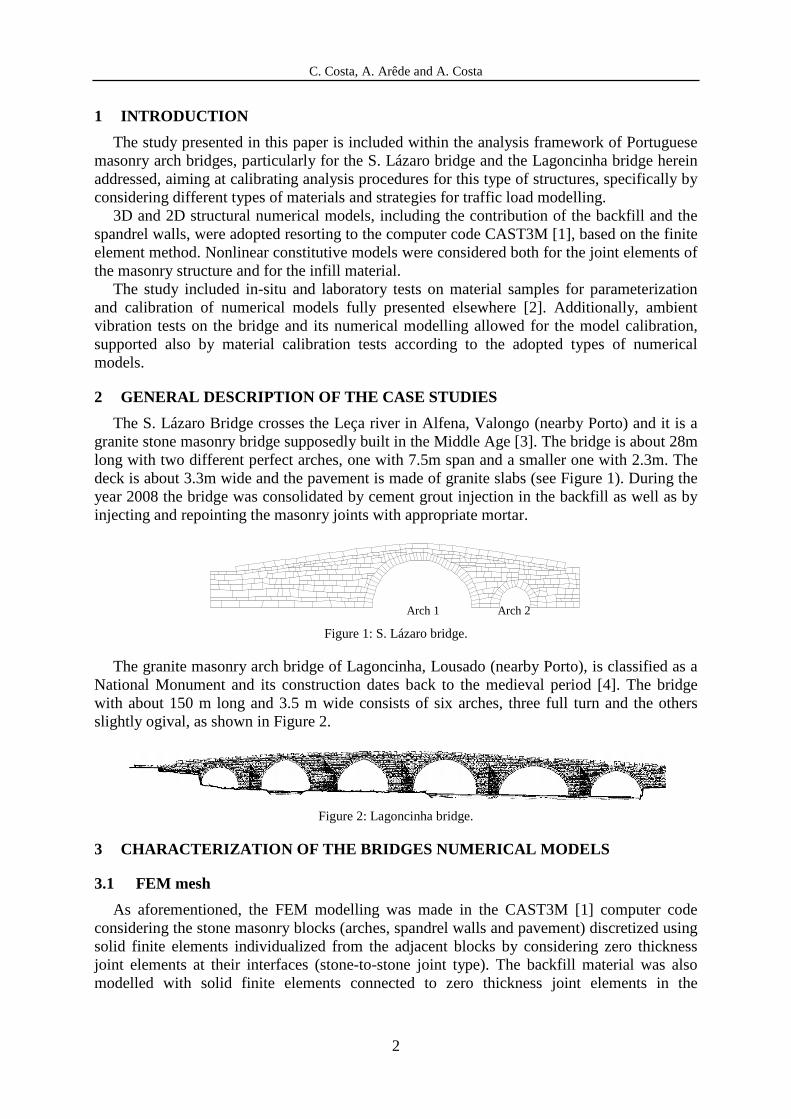
The S. Lázaro Bridge crosses the Leça river in Alfena, Valongo (nearby Porto) and it is a granite stone masonry bridge supposedly built in the Middle Age [3]. The bridge is about 28m long with two different perfect arches, one with 7.5m span and a smaller one with 2.3m. The deck is about 3.3m wide and the pavement is made of granite slabs (see Figure 1). During the year 2008 the bridge was consolidated by cement grout injection in the backfill as well as by injecting and repointing the masonry joints with appropriate mortar.

Figure 1: S. Lázaro bridge.

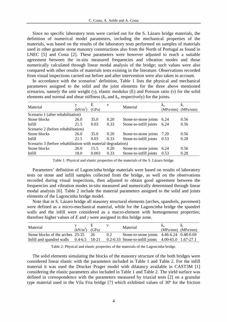
The granite masonry arch bridge of Lagoncinha, Lousado (nearby Porto), is classified as a National Monument and its construction dates back to the medieval period [4]. The bridge with about 150 m long and 3.5 m wide consists of six arches, three full turn and the others slightly ogival, as shown in Figure 2.

Figure 2: Lagoncinha bridge.

3 CHARACTERIZATION OF THE BRIDGES NUMERICAL MODELS

3.1 FEM mesh

As aforementioned, the FEM modelling was made in the CAST3M [1] computer code considering the stone masonry blocks (arches, spandrel walls and pavement) discretized using solid finite elements individualized from the adjacent blocks by considering zero thickness joint elements at their interfaces (stone-to-stone joint type). The backfill material was also modelled with solid finite elements connected to zero thickness joint elements in the

Arch 1 Arch 2


3

interfaces between the infill and blocks of arches, spandrel walls and pavement; in this case, different characteristics were used for this infill-to-stone joint type.

The simulation of the bridges behaviour under the traffic loading was based on 2D and 3D models. The 3D modelling allowed simulating the structural behaviour in both bridge directions (longitudinal and transversal) whereas the 2D modelling aimed at representing the bridge behaviour in the longitudinal direction considering the arch zone under the backfill (central zone, along the bridge longitudinal axis.

3D and 2D finite element meshes of S. Lázaro bridge are illustrated in Figures 3 and 4. The Lagoncinha bridge 3D finite element model is shown in Figure 5.

a) b)

Figure 3: 3D model of the S. Lázaro bridge. a) Solid and b) joint finite elements.

Figure 4: 2D model of the S. Lázaro bridge. Plane (2D) elements (gray) and joint elements (black).

Figure 5: 3D model of the Lagoncinha bridge.

The boundary conditions were set using rigid support to fix the displacements at the bridges base in contact with the riverbed. The horizontal displacements were blocked in the vertical boundary of the abutments.

3.2 Material properties and constitutive models

The S. Lázaro bridge study aimed at calibrating analysis procedures for this type of structures, particularly by considering different types of materials and strategies for traffic load modelling. In this context, three scenarios were considered for the structural materials’ constitution in terms of the type of joints and backfill materials. For one of the scenarios (scenario 1), the analysis aimed at simulating the bridge behaviour after rehabilitation, thus considering the stone block interfaces with filling mortar and the backfill (supposedly) composed by the initially existent granular material and by the added material through cement grout injection. The second scenario (scenario 2) intended to approximate the bridge conditions before a recently made rehabilitation intervention considering the stone block interfaces without filling mortar and the backfill (supposedly) composed by granular material. As for the third scenario (scenario 3), it was intended to simulate the bridge behaviour considering the material constitution with degradation.


4

Since no specific laboratory tests were carried out for the S. Lázaro bridge materials, the definition of numerical model parameters, including the mechanical properties of the materials, was based on the results of the laboratory tests performed on samples of materials used in other granite stone masonry constructions also from the North of Portugal as found in LNEC [5] and Costa [2]. These parameters were however adjusted to reach a suitable agreement between the in-situ measured frequencies and vibration modes and those numerically calculated through linear modal analysis of the bridge; such values were also compared with other results of materials tests existing in the literature. Observations recorded from visual inspections carried out before and after intervention were also taken in account.

In accordance with the scenarios’ definition, Table 1 lists the physical and mechanical parameters assigned to the solid and the joint elements for the three above mentioned scenarios, namely the unit weight (γ), elastic modulus (E) and Poisson ratio (ν) for the solid elements and normal and shear stiffness (kn and ks, respectively) for the joints.

Material γ E ν

Material kn ks

(kN/m3) (GPa) (MPa/mm) (MPa/mm) Scenario 1 (after rehabilitation) Stone blocks 26.0 35.0 0.20 Stone-to-stone joints 6.24 0.56 Infill 21.5 0.03 0.33 Stone-to-infill joints 6.24 0.56 Scenario 2 (before rehabilitation) Stone blocks 26.0 35.0 0.20 Stone-to-stone joints 7.20 0.56 Infill 21.5 0.03 0.33 Stone-to-infill joints 0.53 0.28 Scenario 3 (before rehabilitation with material degradation) Stone blocks 26.0 15.5 0.20 Stone-to-stone joints 6.24 0.56 Infill 18.0 0.003 0.33 Stone-to-infill joints 0.53 0.28

Table 1: Physical and elastic properties of the materials of the S. Lázaro bridge.

Parameters’ definition of Lagoncinha bridge materials were based on results of laboratory tests on stone and infill samples collected from the bridge, as well on the observations recorded during visual inspections, then adjusted to obtain good agreement between the frequencies and vibration modes in-situ measured and numerically determined through linear modal analysis [6]. Table 2 include the material parameters assigned to the solid and joints elements of the Lagoncinha bridge model.

Note that in S. Lázaro bridge all masonry structural elements (arches, spandrels, pavement) were defined as a micro-mechanical material, while for the Lagoncinha bridge the spandrel walls and the infill were considered as a macro-element with homogeneous properties; therefore higher values of E and γ were assigned in this bridge zone.

Material γ E ν Material kn ks (kN/m3) (GPa) (MPa/mm) (MPa/mm)

Stone blocks of the arches 25-35 26 0.2 Stone-to-stone joints 4.46-6.24 0.48-0.69 Infill and spandrel walls 0.4-6.5 18-21 0.2-0.33 Stone-to-infill joints 4.00-65.0 1.67-27.1

Table 2: Physical and elastic properties of the materials of the Lagoncinha bridge.

The solid elements simulating the blocks of the masonry structure of the both bridges were considered linear elastic with the parameters included in Table 1 and Table 2. For the infill material it was used the Drucker Prager model with dilatancy available in CAST3M [1] considering the elastic parameters also included in Table 1 and Table 2. The yield surface was defined in correspondence with the parameters measured by triaxial tests [2] on a granular type material used in the Vila Fria bridge [7] which exhibited values of 30º for the friction


5

angle, 13kPa for the cohesion and 6º for the dilatancy angle. Constitutive parameters assigned of the infill materials of the S. Lázaro and Lagoncinha bridges are shown in Table 3.

Material φ c ψ (º) (kPa) (º)

S. Lázaro bridge Granular material with grout injections after rehabilitation (scenario 1)

33 50 33

Granular material before rehabilitation (scenario 2) 30 13 6 Granular material before rehabilitation with material degradation (scenario 3)

30 0 6

Lagoncinha bridge Granular material 35.5 9.4 6

Table 3: Constitutive parameters of the infill materials of the S. Lázaro and Lagoncinha bridges.

The joint element behaviour was modelled by a nonlinear Coulomb friction model without dilatancy called JOINT_SOFT_CY_T and implemented in the CAST3M package within the context of a previous work [2]. The values considered for the normal stiffness (kn) and tangential stiffness (ks) of the joint elements are also included in Table 1 and Table 2.

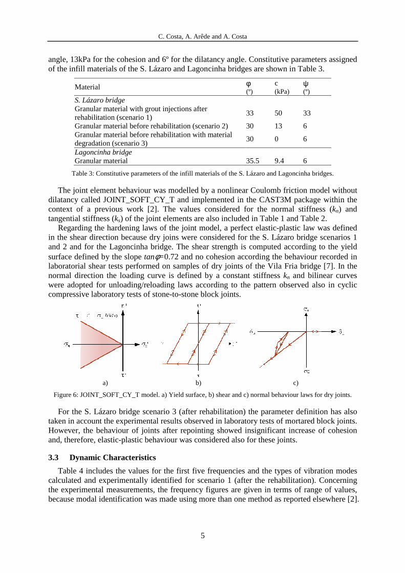
Regarding the hardening laws of the joint model, a perfect elastic-plastic law was defined in the shear direction because dry joins were considered for the S. Lázaro bridge scenarios 1 and 2 and for the Lagoncinha bridge. The shear strength is computed according to the yield surface defined by the slope tanφ=0.72 and no cohesion according the behaviour recorded in laboratorial shear tests performed on samples of dry joints of the Vila Fria bridge [7]. In the normal direction the loading curve is defined by a constant stiffness kn and bilinear curves were adopted for unloading/reloading laws according to the pattern observed also in cyclic compressive laboratory tests of stone-to-stone block joints.

a) b) c)

Figure 6: JOINT_SOFT_CY_T model. a) Yield surface, b) shear and c) normal behaviour laws for dry joints.

For the S. Lázaro bridge scenario 3 (after rehabilitation) the parameter definition has also taken in account the experimental results observed in laboratory tests of mortared block joints. However, the behaviour of joints after repointing showed insignificant increase of cohesion and, therefore, elastic-plastic behaviour was considered also for these joints.

3.3 Dynamic Characteristics

Table 4 includes the values for the first five frequencies and the types of vibration modes calculated and experimentally identified for scenario 1 (after the rehabilitation). Concerning the experimental measurements, the frequency figures are given in terms of range of values, because modal identification was made using more than one method as reported elsewhere [2].


6

However, it is quite apparent that boundary values for each frequency are very close, thus supporting the validity of experimental findings.

The numerical dynamic characteristics were calculated through the detailed 3D model included in Figure 3.

The dynamic characteristics’ results calculated for the scenario 2 (before the rehabilitation) model are also included in Table 4. These results were obtained by the simpler 2D finite element model (Figure 4), therefore not allowing computing transversal modes, but it is clear the frequency drop from scenarios 1 (after the rehabilitation) to 2 (before the rehabilitation).

Table 5 includes the dynamic characteristics’ results in-situ measured and numerically calculated for the Lagoncinha bridge.

Identified Frequencies (Hz) Numerical Frequencies (Hz) Type of vibration mode Scenario 1 Scenario 2

7.70 – 7.80 7.7 - 1st mode (transversal) 10.47 – 10.60 11.7 - 2nd mode (transversal) 12.70 – 12.96 12.9 8.3 3rd mode (longitudinal) 14.20 – 14.47 14.1 - 4th mode (transversal + torsion) 15.37 – 15.71 15.5 11.8 5th mode (vertical)

Table 4: In-situ measured and numerically calculated dynamic characteristics of the S. Lázaro bridge.

Identified Frequencies (Hz) Numerical Frequencies (Hz) Type of vibration mode 3.81 3.92 1st mode (transversal) 4.78 4.69 2nd mode (transversal) 5.48 5.33 3th mode (transversal)

Table 5: In-situ measured and numerically calculated dynamic characteristics of the Lagoncinha bridge.

4 MODELLING OF ROAD TRAFFIC MOVING LOADS

The loads transmitted by vehicles to a bridge consist of moving vertical loads corresponding to each vehicle axel. These loads should be considered as dynamic actions, since, on the one hand, the vehicle traffic with a specific speed on the bridge deck is likely to introduce potentially larger effects than those due to an equal intensity statically applied load (dynamic amplification effects) and, on the other hand, the pavement surface irregularities might trigger impacts on the deck which can further amplify the traffic dynamic effects.

One of the strategies for modelling vehicle loads in the dynamic behaviour of bridges consists on the application of a sequence of vertical concentrated forces. In this case, the vehicle mass is not involved in the numerical model. This load modelling simplification is valid when the vehicle mass is much lower than the total bridge mass and when the speed is not very high. These two conditions are generally met for stone masonry arch bridges but, when this is not the case, the vehicle load model has to be represented by a set of concentrated masses. This procedure implies the system mass updating at each time step of the analysis [8], which renders the numerical simulation more time consuming.

Within the analysis of S. Lázaro and Lagoncinha bridges, the first above mentioned strategy was adopted for studying the dynamic behaviour due to the moving loads. A set of vertical concentrated forces was therefore imposed including the effects of interaction between vehicle wheels and the bridge caused by the pavement surface irregularities and by the vehicle dynamic behaviour.

4.1.1. Bridge-vehicle interaction

The interaction between the wheel and the pavement is considered through a simplified methodology comprising three phases of analysis where the two systems (bridge


7

and vehicle) are studied separately. The first phase consist on the bridge numerical modelling to simulate the vehicle action through a series of concentrated loads applied on the pavement (phase 1). This phase allows evaluating the time history of pavement settlements in accordance with the moving load application points. In the subsequent phase (phase 2), the dynamic analysis of the vehicle is carried out to determine the influence of the pavement irregularities added-up with the previous pavement settlement on the vehicle dynamic behaviour. Therefore, new values of the moving loads are obtained in phase 2, corresponding to the forces (reactions) in the contact wheel/deck surface to be used in the subsequent bridge analysis. Finally, phase 3 consists on a recalculation of the bridge considering the moving load values amplified due to the dynamic behaviour of the vehicle, thereby involving both the interaction vehicles/bridge and the effect of pavement irregularities [9].

4.1.2. Irregularities of the pavement

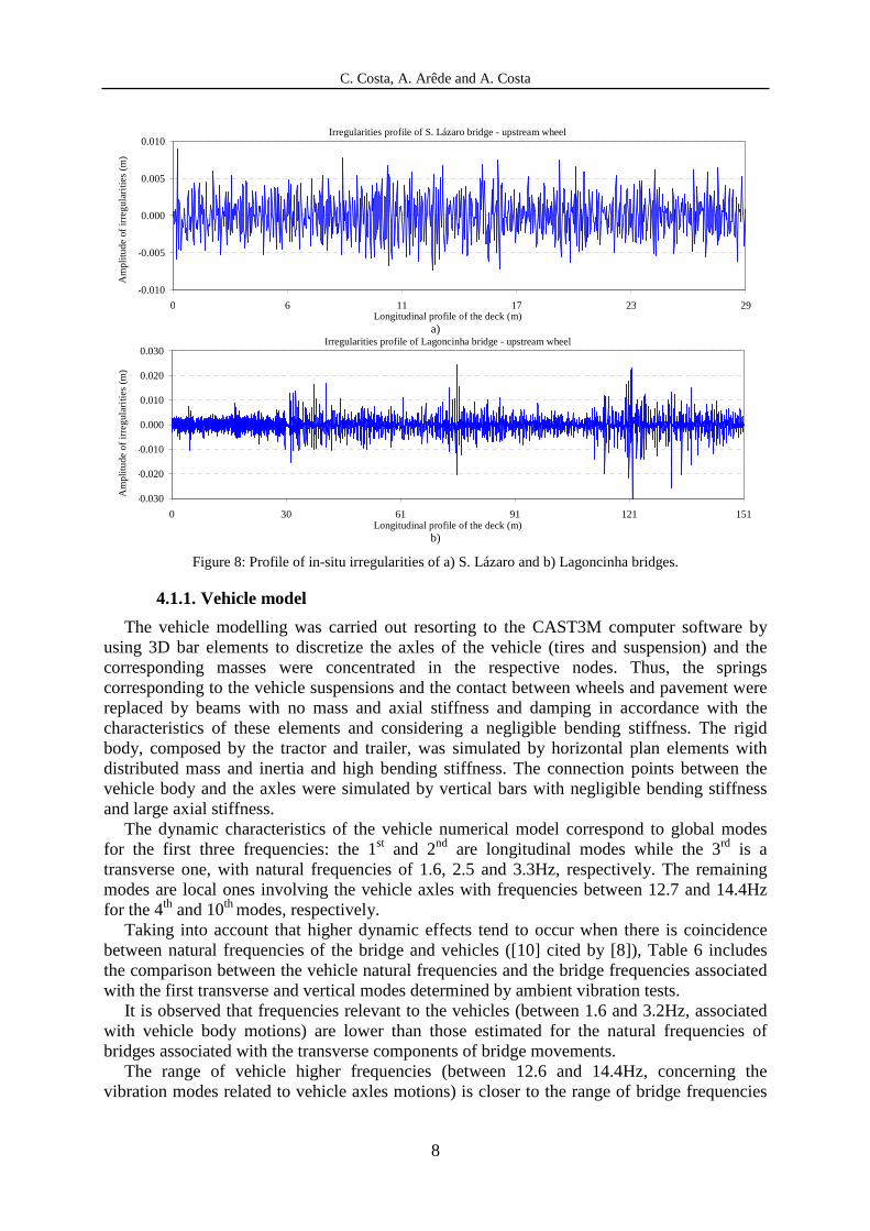
The pavement irregularities of S. Lázaro and Lagoncinha bridges (see Figures 7a and 7b) were recorded along two parallel axes in the deck longitudinal direction by performing a scan with a laser profilograph installed in a commercial vehicle as illustrated in Figure 7c. The scan sampling interval was taken as 0.025m and the acquisition was made during the vehicle ride centred in the deck at an approximately constant speed of 20km/h. A low-pass filter was applied during the acquisition with cut-off frequency corresponding to a wavelength of 100m. The measured signals were corrected adopting usual procedures for such applications [9]. The obtained upstream irregularity profiles in the S. Lázaro and Lagoncinha bridges are shown in Figure 8a and b.

The characterization of the profile amplitude of irregularities in the pavement along the deck of the bridges allowed observing the presence of amplitudes with about 0.015m.

a) b) c)

Figure 7: Pavement surface of a) S. Lázaro and b) Lagoncinha bridges. a) Equipment for measuring the irregularity profile.


8

Am

plitu

de o

f irr

eg

ula

ritie

s (m

) Irregularities profile of S. Lázaro bridge - upstream wheel (Sentido Nascente - Poente)

-0.010

-0.005

0.000

0.005

0.010

0 6 11 17 23 29 Longitudinal profile of the deck (m)

a)

Am

plitu

de o

f irr

eg

ula

ritie

s (m

)

Irregularities profile of Lagoncinha bridge - upstream wheel (Sentido Lousado - Trofa)

-0.030

-0.020

-0.010

0.000

0.010

0.020

0.030

0 30 61 91 121 151 Longitudinal profile of the deck (m)

b)

Figure 8: Profile of in-situ irregularities of a) S. Lázaro and b) Lagoncinha bridges.

4.1.1. Vehicle model

The vehicle modelling was carried out resorting to the CAST3M computer software by using 3D bar elements to discretize the axles of the vehicle (tires and suspension) and the corresponding masses were concentrated in the respective nodes. Thus, the springs corresponding to the vehicle suspensions and the contact between wheels and pavement were replaced by beams with no mass and axial stiffness and damping in accordance with the characteristics of these elements and considering a negligible bending stiffness. The rigid body, composed by the tractor and trailer, was simulated by horizontal plan elements with distributed mass and inertia and high bending stiffness. The connection points between the vehicle body and the axles were simulated by vertical bars with negligible bending stiffness and large axial stiffness.

The dynamic characteristics of the vehicle numerical model correspond to global modes for the first three frequencies: the 1st and 2nd are longitudinal modes while the 3rd is a transverse one, with natural frequencies of 1.6, 2.5 and 3.3Hz, respectively. The remaining modes are local ones involving the vehicle axles with frequencies between 12.7 and 14.4Hz for the 4th and 10th modes, respectively.

Taking into account that higher dynamic effects tend to occur when there is coincidence between natural frequencies of the bridge and vehicles ([10] cited by [8]), Table 6 includes the comparison between the vehicle natural frequencies and the bridge frequencies associated with the first transverse and vertical modes determined by ambient vibration tests.

It is observed that frequencies relevant to the vehicles (between 1.6 and 3.2Hz, associated with vehicle body motions) are lower than those estimated for the natural frequencies of bridges associated with the transverse components of bridge movements.

The range of vehicle higher frequencies (between 12.6 and 14.4Hz, concerning the vibration modes related to vehicle axles motions) is closer to the range of bridge frequencies


9

relative to vertical modes, but the vehicle response has less energy content for this range of frequencies, which means that the higher energy content recorded in the vehicle response deviates from resonance with the bridge structure.

Mode type: 1st long. 2nd long. 1st trans. 1st vert. 7th vert. Mode type: 1st trans. 1st vert.

4-axle truck 1.6 2.5 3.3 12.7 14.4 Lagoncinha bridge 3.9 11.3

S. Lázaro bridge 7.7 15.5

Table 6: Frequency (Hz) and mode types of vehicles and masonry arch bridges

Considering the measured roughness distribution, the range of irregularities' wavelengths (λ) likely to contribute for the vehicle excitation in the frequency (f) interval from 1.6 to 14.4 Hz and assuming vehicle speed (ν), between 12 and 90 km/h, corresponds to λ within 0.23m and 6.15m as obtained by the expression f/v=λ ).

The observation of the spectral densities determined by Fast Fourier Transform (FFT) of the roughness profile showed that the largest amplitude of the spectra occurs in the range of wavelengths between 0.08m and 0.2m, thus shifted away from the range of wavelengths most significant for the vehicle excitation.

5 RESULTS ANALYSIS OF THE BRIDGES BEHAVIOUR UNDER THE ROAD TRAFFIC CONSIDERING DIFFERENT APPROACHES

5.1 Bridge behaviour under road traffic moving loads

In order to evaluate the result sensitivity of the bridge response to the vehicle speed, effects of irregularities and type of calculation considered in the bridge numerical simulation, particularly concerning static vs. dynamic and linear vs. nonlinear analysis, several analysis were performed to study the influence of moving loads on the bridges.

For the S. Lázaro bridge, in case I linear static analysis was performed in two phases (1 and 3) of the structural calculation. In case II, the dynamic behaviour was activated in both phases, but assuming a linear material. In cases III and IV the material nonlinear behaviour was taken into account, case III involving static calculations and case IV including also the activation of the dynamic behaviour. For each case, the following four speed values were considered: 13, 30, 60 and 90km/h.

For the Lagoncinha bridge in the first calculation phase (phase 1) dynamic analyses were carried out considering the linear velocities of 20, 30, 60 and 90km/h.

In the analyses including the roughness effects (phase 3) three calculation options were considered. One of the options held also linear dynamic analysis. In two cases, the nonlinear behaviour of materials was considered, in one case, performing nonlinear dynamic analysis and, on the other, non-linear static analysis. The speed of 90km/h was considered in the cases where the dynamic behaviour was activated in phase 3. The option for this speed value drive from the fact that a smaller number of steps is needed for the load history and, consequently, the required time for the 3D bridge analysis decreased.

In all cases the study of vehicle response (phase 2) was based on linear dynamic analysis. Numerical integration of dynamic equations was made resorting to the Newmark scheme

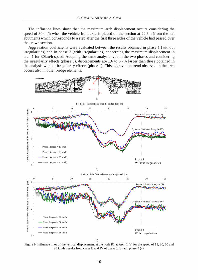
and the non-linearity was solved using the classical Newton-Raphson method. Figure 9 shows the results in terms of the influence lines of de vertical displacement on the

principal arch of the S. Lázaro bridge (at the node P1 for which the maximum arch vertical displacement was found). Dynamic linear and nonlinear analyses were performed in the two calculation phases (phase 1 - without irregularities and phase 3 - with irregularities) considering the 2D bridge model shown in Figure 4.


10

The influence lines show that the maximum arch displacement occurs considering the speed of 30km/h when the vehicle front axle is placed on the section at 22.6m (from the left abutment) which corresponds to a step after the first three axles of the vehicle had passed over the crown section.

Aggravation coefficients were evaluated between the results obtained in phase 1 (without irregularities) and in phase 3 (with irregularities) concerning the maximum displacement in arch 1 for 30km/h speed. Adopting the same analysis type in the two phases and considering the irregularity effects (phase 3), displacements are 1.6 to 6.7% larger than those obtained in the analysis without irregularity effects (phase 1). This aggravation trend observed in the arch occurs also in other bridge elements.

+

P1

Arco1 S1

a)

b)

c)

Figure 9: Influence lines of the vertical displacement at the node P1 at Arch 1 (a) for the speed of 13, 30, 60 and 90 km/h, results from cases II and IV of phase 1 (b) and phase 3 (c).

1

2

3

0 5 10 15 20 25 30 35

Posição do Eixo 1 ao longo do percurso (m)

De

slo

cam

ento

ve

rtic

al d

o n

ó P

1 d

o A

rco

1

(mm

)

Fase 3 (velc = 12.8 km/h)

Fase 3 (velc = 30 km/h)



Análise Dinâmica Linear (II)

Análise Dinâmica Não Linear (IV)

Phase 3 With irregularities

Phase 3 (speed = 13 km/h)




1

2

3

0 5 10 15 20 25 30 35

Posição do Eixo 1 ao longo do percurso (m)

Des

loca

me

nto

ve

rtic

al d

o n

ó P

1 d

o A

rco 1

(m

m)

Fase 1 (velc = 12.8 km/h)




Análise Dinâmica Linear (II)

Análise Dinâmica Não Linear (IV)

Phase 1 Without irregularities





Position of the front axle over the bridge deck (m)

Ve

rtic

al d

ispl

ace

me

nt o

f th

e n

ode

P1

of

the

arc

h 1

(mm

)


Dynamic Linear Analysis (II)

Dynamic Non Linear Analysis (IV)

Dynamic Linear Analysis (II)

Dynamic Nonlinear Analysis (IV)

Dynamic Nonlinear Analysis (IV)

Arch 1

Ve

rtic

al d

ispl

ace

me

nt o

f th

e n

ode

P1

of

the

arc

h 1

(mm

)


11

The maximum displacement of 2.6 mm was obtained in phase 3 (with irregularities) considering the analysis where the nonlinear behaviour of materials is activated in the two phases. Comparing the maximum displacement obtained in the nonlinear static analysis with the effects of irregularities (phase 3) and the displacement obtained in the linear static analysis without the effects of irregularities (phase 1) it was found an aggravation of about 37.4%.

The comparison of the influence line obtained from nonlinear dynamic analysis with that obtained from nonlinear static analysis shows that the displacement of node P1 is lower in the latter case only when loads are at the bridge entrance. By contrast, in the remaining path, the results are quite similar to those obtained considering dynamic behaviour, thus showing that the consideration of the dynamic calculation has little influence on the response of this bridge.

The results show also greater dynamic component in the vertical displacement of the node P1 when the moving loads are in the entry and exit zones of the bridge, rather than in the arch neighbourhood. Therefore, considering the position of the moving loads in relation to the node P1, it is concluded that the vibration recorded on the arch follows the vibration transmitted by the infill.

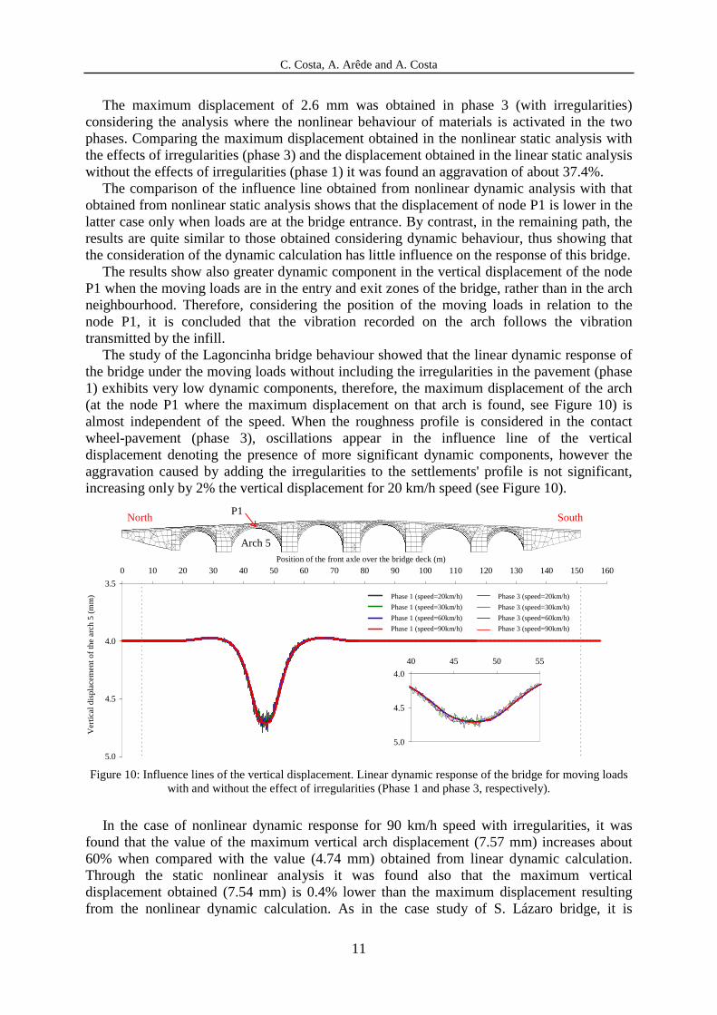
The study of the Lagoncinha bridge behaviour showed that the linear dynamic response of the bridge under the moving loads without including the irregularities in the pavement (phase 1) exhibits very low dynamic components, therefore, the maximum displacement of the arch (at the node P1 where the maximum displacement on that arch is found, see Figure 10) is almost independent of the speed. When the roughness profile is considered in the contact wheel-pavement (phase 3), oscillations appear in the influence line of the vertical displacement denoting the presence of more significant dynamic components, however the aggravation caused by adding the irregularities to the settlements' profile is not significant, increasing only by 2% the vertical displacement for 20 km/h speed (see Figure 10).


Ve

rtic

al d

ispl

ace

me

nt o

f th

e a

rch

5 (m

m)

3.5

4.0

4.5

5.0

0 10 20 30 40 50 60 70 80 90 100 110 120 130 140 150 160

Fase 1 (velc = 20 km/h) Fase 3 (velc = 20 km/h)Fase 1 (velc = 30 km/h) Fase 3 (velc = 30 km/h)

Fase 1 (velc = 60 km/h) Fase 3 (velc = 60 km/h)Fase 1 (velc = 90 km/h) Fase 3 (velc = 90 km/h)

4.0

4.5

5.0

40 45 50 55

Figure 10: Influence lines of the vertical displacement. Linear dynamic response of the bridge for moving loads with and without the effect of irregularities (Phase 1 and phase 3, respectively).

In the case of nonlinear dynamic response for 90 km/h speed with irregularities, it was found that the value of the maximum vertical arch displacement (7.57 mm) increases about 60% when compared with the value (4.74 mm) obtained from linear dynamic calculation. Through the static nonlinear analysis it was found also that the maximum vertical displacement obtained (7.54 mm) is 0.4% lower than the maximum displacement resulting from the nonlinear dynamic calculation. As in the case study of S. Lázaro bridge, it is

Arch 5

P1 North South

Phase 1 (speed=20km/h)

Phase 1 (speed=30km/h) Phase 1 (speed=60km/h) Phase 1 (speed=90km/h)

Phase 3 (speed=20km/h)

Phase 3 (speed=30km/h) Phase 3 (speed=60km/h) Phase 3 (speed=90km/h)


12

observed that the consideration of material nonlinear behaviour produces a significant effect on the maximum displacement of the bridge main arch and less influence is found when the bridge dynamic behaviour is taken in account.

In order to evaluate the influence of the loading history on the response of the two bridges, the maximum vertical displacement of the arches obtained from the nonlinear dynamic calculation with irregularities nldy

vd are compared in Table 7 with similar results obtained from a nonlinear static analysis nlest

vd , but considering identical positions and values for the static loads. It is verified that the vertical displacement obtained considering the load history is 22% and 12% larger than that determined by static analysis of the S. Lázaro and Lagoncinha bridges, respectively, allowing the conclude that the entire history of loading is important to evaluate the structural response.

nlest

vd nldyvd

S. Lázaro bridge (arch 1) 2.11 2.58 (+22%) Lagoncinha bridge (arch 5) 6.70 7.57 (+12%)

Table 7: Maximum vertical displacement of the arch (mm). Static load position vs. moving loading model.

5.2 Bridge behaviour under incremental static loads

Considering the vehicle at the most unfavourable load position for the arch identified previously from the analysis of the bridge considering the moving loading, this section focuses on the relevant aspects of the bridge response considering the nonlinear behaviour of joints and infill and intensity load levels (multipliers) of one and twice the nominal vehicle load.

The evolution of the response parameters in terms of maximum vertical displacement and principal stresses on the arch blocks, concerning the effect of the bridge weight and the intensity levels of the vehicle load of 1P and 2P, can be evaluated through the results included in Table 8. For these load levels, Table 8 includes the response parameters of the joints of the arch in terms of normal and shear stresses (maximum) and the corresponding maximum values of the normal and tangential deformations.

Comparing the results of 2D and 3D simulations, good agreement is observed in the longitudinal direction behaviour parameters. Given the effects of the dead load, it is verified that opening of transverse joints between the arch blocks does not occur. This also means that no incursions occur in the nonlinear range for the normal direction; since these joints have zero tensile strength, shear yielding is not triggered as well.

In the longitudinal joints of the arch (modelled only in 3D models) there were opening deformations. In the bridge transverse direction, that fact indicates the effect on the arch which induces impulses in the spandrels, leading to opening movements and decompression in the transverse direction. This aspect is not represented in 2D modelling and is not well reproduced in 3D linear calculation, because in the latter the stress transmission is kept even when separation occurs at the interfaces between the bridge elements. In the longitudinal arch joints, plastic components of the sliding joint deformation (shear yielding) are also observed.

The inclusion of the vehicle action shows that, in the arch transverse joints, normal opening deformations occur in tensioned areas but without forming a hinge mechanism, which is consistent with the smooth functioning of the arch in this scenario.

The existence of plastic deformations in the infill, only in a limited area under the loading in both 3D and 2D modelling, also adds to the confirmation of the smoothening effect of the infill.


13

3D 2D 3D 2D Loads +

1σ −3σ vd +

1σ −2σ vd máx

nσ minnσ máx

nδ máxnσ min

nσ máxnδ

DL 0.12 -0.48 1.35 0.04 -0.57 1.48 (t) (l)

-0.03 0.00

-0.40 -0.02

0.00 0.08

-0.01 -

-0.43 -

0.00 -

DL+1 x 4-axles truck 0.20 -0.65 2.42 0.07 -0.69 2.50 (t) (l)

0.00 0.00

-0.61 -0.05

0.04 0.11

0.00 -

-0.59 -

0.05 -

DL+2 x 4-axles truck 0.31 -0.94 3.61 0.12 -0.90 3.70 (t) (l)

0.00 0.00

-0.86 -0.09

0.09 0.02

0.00 -

-0.85 -

-0.06 -

DL – Dead load; (t) Transversal joints; (l) Longitudinal joints; - joints not considered in the 2D model

Table 8: Principal stresses in blocks and joints (MPa) and maximum displacement (mm) and deformations in joints of arch 1. Results from 3D and 2D models.

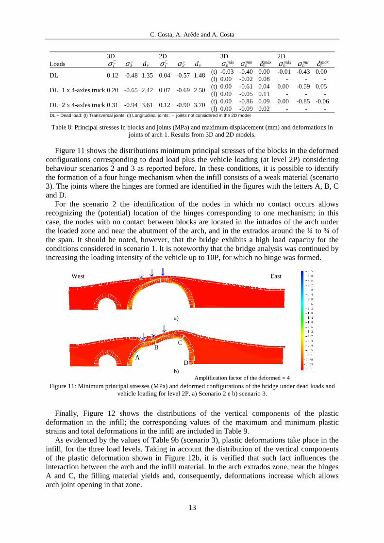
Figure 11 shows the distributions minimum principal stresses of the blocks in the deformed configurations corresponding to dead load plus the vehicle loading (at level 2P) considering behaviour scenarios 2 and 3 as reported before. In these conditions, it is possible to identify the formation of a four hinge mechanism when the infill consists of a weak material (scenario 3). The joints where the hinges are formed are identified in the figures with the letters A, B, C and D.

For the scenario 2 the identification of the nodes in which no contact occurs allows recognizing the (potential) location of the hinges corresponding to one mechanism; in this case, the nodes with no contact between blocks are located in the intrados of the arch under the loaded zone and near the abutment of the arch, and in the extrados around the ¼ to ¾ of the span. It should be noted, however, that the bridge exhibits a high load capacity for the conditions considered in scenario 1. It is noteworthy that the bridge analysis was continued by increasing the loading intensity of the vehicle up to 10P, for which no hinge was formed.

a)

b)

Amplification factor of the deformed = 4

Figure 11: Minimum principal stresses (MPa) and deformed configurations of the bridge under dead loads and vehicle loading for level 2P. a) Scenario 2 e b) scenario 3.

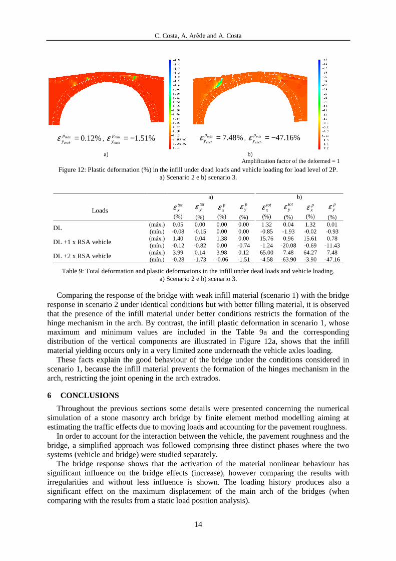
Finally, Figure 12 shows the distributions of the vertical components of the plastic deformation in the infill; the corresponding values of the maximum and minimum plastic strains and total deformations in the infill are included in Table 9.

As evidenced by the values of Table 9b (scenario 3), plastic deformations take place in the infill, for the three load levels. Taking in account the distribution of the vertical components of the plastic deformation shown in Figure 12b, it is verified that such fact influences the interaction between the arch and the infill material. In the arch extrados zone, near the hinges A and C, the filling material yields and, consequently, deformations increase which allows arch joint opening in that zone.

A

B C

D

West East


14

%12.0=máx

ench

pyε , %51.1−=mín

ench

pyε

%48.7=máx

ench

pyε , %16.47−=mín

ench

pyε

a) b)

Amplification factor of the deformed = 1

Figure 12: Plastic deformation (%) in the infill under dead loads and vehicle loading for load level of 2P. a) Scenario 2 e b) scenario 3.

a)

b)

Loads totxε

(%)

totyε

(%)

pxε

(%)

pyε

(%)

totxε

(%)

totyε

(%)

pxε

(%)

pyε

(%)

DL (máx.) 0.05 -0.08

0.00 -0.15

0.00 0.00

0.00 0.00

1.32 -0.85

0.04 -1.93

1.32 -0.02

0.01 -0.93 (mín.)

DL +1 x RSA vehicle (máx.) 1.40 -0.12

0.04 -0.82

1.38 0.00

0.00 -0.74

15.76 -1.24

0.96 -20.08

15.61 -0.69

0.78 -11.43 (mín.)

DL +2 x RSA vehicle (máx.) 3.99 -0.28

0.14 -1.73

3.98 -0.06

0.12 -1.51

65.00 -4.58

7.48 -63.90

64.27 -3.90

7.48 -47.16 (mín.)

Table 9: Total deformation and plastic deformations in the infill under dead loads and vehicle loading. a) Scenario 2 e b) scenario 3.

Comparing the response of the bridge with weak infill material (scenario 1) with the bridge response in scenario 2 under identical conditions but with better filling material, it is observed that the presence of the infill material under better conditions restricts the formation of the hinge mechanism in the arch. By contrast, the infill plastic deformation in scenario 1, whose maximum and minimum values are included in the Table 9a and the corresponding distribution of the vertical components are illustrated in Figure 12a, shows that the infill material yielding occurs only in a very limited zone underneath the vehicle axles loading.

These facts explain the good behaviour of the bridge under the conditions considered in scenario 1, because the infill material prevents the formation of the hinges mechanism in the arch, restricting the joint opening in the arch extrados.

6 CONCLUSIONS

Throughout the previous sections some details were presented concerning the numerical simulation of a stone masonry arch bridge by finite element method modelling aiming at estimating the traffic effects due to moving loads and accounting for the pavement roughness.

In order to account for the interaction between the vehicle, the pavement roughness and the bridge, a simplified approach was followed comprising three distinct phases where the two systems (vehicle and bridge) were studied separately.

The bridge response shows that the activation of the material nonlinear behaviour has significant influence on the bridge effects (increase), however comparing the results with irregularities and without less influence is shown. The loading history produces also a significant effect on the maximum displacement of the main arch of the bridges (when comparing with the results from a static load position analysis).


15

The results show that the dynamic behaviour activation does not produce a significant effect on the maximum displacement of the main arch of the bridges. The study also allowed concluding that the dynamic effects are mainly due to the vehicle dynamic response, with negligible influence on the dynamic response of the bridge.

REFERENCES

[1] CEA, Manuel d'utilisation de CAST3M. by P. Pasquet, Commissariat à l'Énergie Atomique, 2003. http://www.cast3m.cea.fr .

[2] Costa, C., Análise numérica e experimental do comportamento estrutural de pontes em arco de alvenaria de pedra. PhD thesis, FEUP, 2009. (in Portuguese, available at site NCREP)

[3] IHRU, Ponte de São Lázaro. Sistema de Informação para o Património Arquitectónico - SIPA. Nº IPA: PT011315010002, 1998. http://www.monumentos.pt/Monumentos/.

[4] DGEMN, Ponte da Lagoncinha, Boletim da Direcção Geral dos Edifícios e Monumentos Nacionais, MOP, 1957. (in Portuguese)

[5] LNEC, Ensaios de Mecânica das Rochas na Igreja do Mosteiro da Serra do Pilar. Technical Report. Laboratório Nacional de Engenharia Civil, 2000. (in Portuguese)

[6] Costa, C., Arêde, A. and Costa, A., Dynamic Characterization of a Masonry Arch Bridge. 1st International Operational Modal Analysis Conference. AU-SVS-B&K, Copenhagen, 2005.

[7] Costa, C., Costa, P., Arêde, A. and Costa, A., Structural design, modelling, material testing and construction of a new stone masonry arch bridge in Vila Fria, Portugal. 5th International Conference on Arch Bridges (ARCH’07), 2007.

[8] Calçada, R, Avaliação experimental e numérica de efeitos dinâmicos de cargas de tráfego em pontes rodoviárias. PhD thesis, FEUP, 2001. (in Portuguese, available at http://aleph.fe.up.pt/)

[9] Costa, C., Arêde, A. and Costa, A., Numerical simulation of stone masonry arch bridges behaviour under road traffic moving loads 6th International Conference on Arch Bridges (ARCH’10), 2010

[10] OCDE, Dynamic interaction between vehicles and infrastructure experiment (DIVINE). Paris, Organisation for Economic Co-operation and Development, 1998.

DETAILED FEM MODELLING OF STONE MASONRY ARCH BRIDGES UNDER ROAD TRAFFIC MOVING LOADScongress.cimne.com/eccomas/proceedings/compdyn2011/... · moving loads and taking in account the

Documents