Designing image-based control systems considering workload ...

Designing image-based control systems considering workload variations

Sajid Mohamed, Asad Ullah Awan, Dip Goswami and Twan Basten

Abstract— We consider the problem of designing an Image-Based Control (IBC) application mapped to a multiprocessorplatform. Sensing in IBC consists of compute-intensive imageprocessing algorithms whose execution times are dependenton image workload. The challenge is that the IBC systemshave a high (worst-case) workload with significant workloadvariations. Designing controllers for such IBC systems typicallyconsider the worst-case workload that results in a long sensingdelay with suboptimal quality-of-control (QoC). The challengeis: how to improve the QoC of IBC for a given multiprocessorplatform allocation?

We present a controller synthesis method based on aMarkovian jump linear system (MJLS) formulation consid-ering workload variations. Our method assumes that systemknowledge is available for modelling the workload variationsas a Markov chain. We compare the MJLS-based methodwith two relevant control paradigms - LQR control consideringworst-case workload, and switched linear control - with respectto QoC and available system knowledge. Our results showthat taking into account workload variations in controllerdesign benefits QoC. We then provide design guidelines on thecontrol paradigm to choose for an IBC application given therequirements and the system knowledge.

I. INTRODUCTION

Image-Based Control (IBC) systems are a class of data-intensive feedback control systems having camera(s) as thesensor (see Fig. 1). IBC has become popular with the adventof efficient image-processing systems and low-cost CMOScameras with high resolution [1][2]. The combination of thecamera and image processing (sensing) gives necessary in-formation on parameters such as relative position, geometry,relative distance, depth perception and tracking of the object-of-interest. This enables the effective use of low-cost camerasensors to enable new functionality or replace expensivesensors in cost-sensitive industries like automotive [1][3][4].

A typical implementation of an IBC system uses linearquadratic regulator (LQR) control [5] and considers theworst-case workload [4]. However, this leads to a longsensing delay, poor effective resource utilisation in themultiprocessor platform, and suboptimal quality-of-control(QoC) [6]. Fig. 2 illustrates these challenges. The cameracaptures an image stream at a fixed frame rate per sec-ond (fps). The execution times of the compute-intensive

This research has received funding from the European Union’s Horizon2020 Framework Programme for Research and Innovation under grantagreement no 674875 (oCPS).

S. Mohamed, D. Goswami and T. Basten are with the Elec-tronic Systems group, Department of Electrical Engineering, Eind-hoven University of Technology, Eindhoven, The Netherlands. Email:{s.mohamed,d.goswami,a.a.basten}@tue.nl.

A. U. Awan is with the Department of Electrical and Computer Engineer-ing, Technical University of Munich, D-80290 Munich, Germany. Email:[email protected].

Sensing and

processing

Control

computationActuation

Dynamic system

(continuous time)

Embedded platform (discrete-time)

Camera

Fig. 1: An image-based control (IBC) system: block diagram

processing (sensing) of the image stream depend on imageworkload variations. The workload variations occur due toimage content and result in a wide range between best-caseand the worst-case image processing times.

The workload variations can, however, be statisticallyanalysed, e.g. as a PERT distribution [7] or discrete-timeMarkov chain (DTMC) [8], from observed data and can bemodelled as workload scenarios [6]. The workload scenarioscan be modelled (e.g. as a task graph or a data flow graph),analysed (for timing) and then mapped to a multiprocessorplatform. A system scenario abstracts multiple workloadscenarios having the same sampling period as determinedby platform constraints. An optimal mapping and controllermay then be designed for each system scenario.

For efficiently designing IBC systems, we should considerthe workload variations and the given platform allocation.An ideal design approach should: (i) identify, model andcharacterise the workload scenarios; (ii) find optimal map-pings for these workload scenarios for the given platformallocation; (iii) identify optimal system scenarios; and (iv)design a controller with high overall QoC for the chosensystem scenarios. One of the critical aspects here is: whatis a good metric to define the QoC for the application?A vision-guided braking application requires a fast settlingtime, whereas an automotive vision-based lateral control [9]application requires to minimise the reference tracking error.

In [6], a scenario- and platform-aware design (SPADe)approach is introduced for designing IBC systems. SPADecharacterises a set of frequently occurring workload sce-narios, identifies a set of system scenarios that abstractmultiple workload scenarios based on platform constraints,and designs a switched linear control system for these systemscenarios to improve the settling time. However, a challengein SPADe is the difficulty to guarantee stability for theresulting switched system [2]. In case of failure to guaranteestability, SPADe would result in LQR control for the worst-case workload scenario.

The contributions of the current paper are as follows:

• We present an alternate controller synthesis methodbased on a Markovian jump linear system (MJLS) for-

mulation. Our synthesis method involves the followingsteps. (i) Modelling workload variations as a DTMC,(ii) system scenario identification, and (iii) controllerdesign and implementation. The motivation to choosethe MJLS approach [10] over other standard sampled-data linear control design techniques [11] is that it doesnot require us to know the exact sequence of incomingsample times due to the workload variations apriori.

• We provide design guidelines on the applicability ofcontrol design methods for given requirements, im-plementation constraints and system knowledge. Forthis, we compare the three control paradigms - opti-mal control design using LQR, switched linear controldesign [2] using SPADe [6], and controller synthesisusing the MJLS formulation - for IBC system designwith respect to QoC while taking into account availablesystem knowledge and implementation constraints, i.e.camera fps, platform allocation and mapping. Notethat we cannot compare with adaptive [12] or modelpredictive control [13] approaches since we do not knowthe exact sequence of occurrence of incoming sampletimes due to the workload variations apriori.

This paper is organised as follows: We explain the embed-ded IBC system setting, the motivating case study, controllerimplementation and our controller configurations in Sec. II.In Sec. III, modelling the IBC application, system mapping,system scenario identification and configuration switchingare discussed. The control problem and the QoC metricswe consider are explained in Sec. IV. Sec. V explains themethod for designing the controllers we consider, includingthe controller synthesis method using the MJLS formulationthat we present in this work. Section VI presents the resultsand observations of our comparison of control paradigms andprovides design guidelines. Conclusion and future work aresummarised in Section VII.

II. EMBEDDED IMAGE-BASED CONTROL

We consider a setting for an IBC system as shown inFig. 1. Our sensor is the camera module that captures theimage stream. The image stream is then fed to an embeddedplatform, e.g a multiprocessor system-on-chip (MPSoC), ata fixed frame rate per second (fps), e.g. 30 fps. The tasks inour IBC application - compute-intensive image sensing andprocessing (S), control computation (C) and actuation (A) -are then mapped to run on this MPSoC.

Motivating case study: We consider the motivatingcase study of vision-based lateral control of a vehicle [9],where the vehicle should follow a lane autonomously (lane-keeping). The image (sensing and) processing algorithmprocesses the camera frames and computes the lateraldeviation at a set look-ahead distance. The controller takesthe lateral deviation as the sensor input, computes thesteering angle and actuates the steering to follow the lane.

best-case

CS A CS A

100 time (ms)0 200

CS A

Average workload Minimal workload

workload

distribution

worst-case

rarely happens

idle time

30 fps

idle time

frequent idle resource time – inefficient utilisation

dropped frames

Fig. 2: Illustration of IBC system implementation andchallenges for LQR control design considering worst-caseworkload. (S: sensing and image processing, C: controlcomputation and A: actuation, see Fig. 1.)

A. LTI systems

We consider a linear time-invariant (LTI) system givenby:

xc(t) = Acxc(t) +Bcu(t), (II.1)yc(t) = Ccxc(t),

where xc(t) ∈ Rn represents the state, yc(t) ∈ R representsthe output and u(t) ∈ R represents the control input of thesystem at any time t ∈ R≥0. Ac, Bc and Cc represent thestate, input and output matrices of the system, respectively.For our case study, we consider the model in [9], where

Ac =

−10.06 −12.99 0 0 0

1.096 −11.27 0 0 0−1.000 −15.00 0 15 0

0 −1.000 0 0 150 0 0 0 0

, Bc =

75.4750.14

000

.The five system states are - lateral velocity, yaw rate of

of vehicle, lateral deviation from the desired centerline pointat look-ahead distance yL, the angle between the tangent tothe road and vehicle orientation, and the curvature of theroad at the look-ahead distance. The control input u(t) isthe front wheel steering angle δf and the output yc(t) is thelook-ahead distance yL leading to Cc = [0 0 1 0 0].

B. Discrete-time control implementation

Implementation of an IBC system involves the executionof three sequential tasks: sensing and processing (S), controlcomputation (C) and actuation (A). These tasks repeat; letthe start and finish times of the k-th instance be given byts(.) and tf (.), respectively. The execution times of Sk, Ck

and Ak (the k-th instance) are given by,

ekT = tf (T k)− ts(T k)

where T ∈ {S,C,A}. The interval between two consecutiveexecutions of sensing tasks Sk and Sk+1 is then the samplingperiod hk for the k-th instance.

hk = ts(Sk+1)− ts(Sk)

Within each sampling period hk, the control operations areexecuted sequentially (i.e., Sk → Ck → Ak). In addition, thetime interval between the starting time of Sk and finishing

time of Ak is then the sensor-to-actuator delay τk for thek-th instance.

τk = tf (Ak)− ts(Sk).

We consider a time-triggered implementation for actuationtask A to guarantee constant τk. A data-driven implementa-tion approach is considered for S and C. Each workloadscenario sk is annotated with pair (hk, τk) that models thesampling period and delay associated with it. A zero-ordersample-and-hold approach can then be used to discretize thesystem based on the workload scenario sk. Eq. (II.1) can bereformulated as follows:

x[k + 1] = Askx[k] +B0,sku[k] +B1,sku[k − 1],

y[k] = Ccx[k] (II.2)

where,

Ask = eAchk , (II.3)

B0,sk =

∫ hk−τk

0

eAcsds ·Bc, B1,sk =

∫ hk

hk−τkeAcsds ·Bc

In Eq. (II.2), we assume that u[−1] = 0 for k = 0. Wedefine new system states z[k] =

[x[k] u[k − 1]

]Twith

z[0] =[x[0] 0

]Tto obtain a higher-order augmented

system as follows:

z[k + 1] = Aaug,skz[k] +Baug,sku[k] (II.4)

where,

Aaug,sk =

[Ask B1,sk

0 0

], Baug,sk =

[B0,sk

I

]. (II.5)

0 and I represent the zero and identity matrices of appro-priate dimensions. A check for controllability [5] is donefor this augmented system. If the system is not controllable,controllability decomposition is done to obtain a controllablesubsystem.

C. Control law and control configurations

The control input u[k] is a state feedback controller ofthe following form,

u[k] = Fskz[k] + Ff,skrref (II.6)

where Fsk is the state feedback gain and Ff,sk is thefeedforward gain both designed for the workload scenario sk.rref is the reference value for the controller. The approacheswe use for designing the gains are explained in Sec. V.

For each workload scenario sk, we then define a controlconfiguration χsk as a tuple χsk = (hsk , τsk , Fsk , Ff,sk).

III. IBC MODEL, MAPPING AND CONFIGURATIONS

In this section, we explain how we model our IBCapplication, characterise the workload, map our applicationto platform and identify our system scenarios. We alsoexplain why there is a switching behaviour.

A

ea

1

C

ec

RoIP

ep

RoIM

em

RoID

ed

RoIP

ep

y2 y2

y1y1

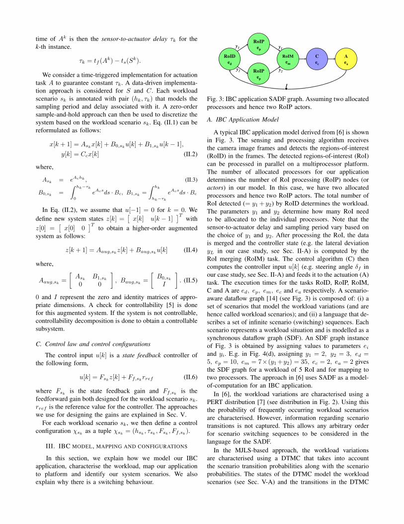
Fig. 3: IBC application SADF graph. Assuming two allocatedprocessors and hence two RoIP actors.

A. IBC Application Model

A typical IBC application model derived from [6] is shownin Fig. 3. The sensing and processing algorithm receivesthe camera image frames and detects the regions-of-interest(RoID) in the frames. The detected regions-of-interest (RoI)can be processed in parallel on a multiprocessor platform.The number of allocated processors for our applicationdetermines the number of RoI processing (RoIP) nodes (oractors) in our model. In this case, we have two allocatedprocessors and hence two RoIP actors. The total number ofRoI detected (= y1 + y2) by RoID determines the workload.The parameters y1 and y2 determine how many RoI needto be allocated to the individual processors. Note that thesensor-to-actuator delay and sampling period vary based onthe choice of y1 and y2. After processing the RoI, the datais merged and the controller state (e.g. the lateral deviationyL in our case study, see Sec. II-A) is computed by theRoI merging (RoIM) task. The control algorithm (C) thencomputes the controller input u[k] (e.g. steering angle δf inour case study, see Sec. II-A) and feeds it to the actuation (A)task. The execution times for the tasks RoID, RoIP, RoIM,C and A are ed, ep, em, ec and ea respectively. A scenario-aware dataflow graph [14] (see Fig. 3) is composed of: (i) aset of scenarios that model the workload variations (and arehence called workload scenarios); and (ii) a language that de-scribes a set of infinite scenario (switching) sequences. Eachscenario represents a workload situation and is modelled as asynchronous dataflow graph (SDF). An SDF graph instanceof Fig. 3 is obtained by assigning values to parameters eiand yi. E.g. in Fig. 4(d), assigning y1 = 2, y2 = 3, ed =5, ep = 10, em = 7×(y1 +y2) = 35, ec = 2, ea = 2 givesthe SDF graph for a workload of 5 RoI and for mapping totwo processors. The approach in [6] uses SADF as a model-of-computation for an IBC application.

In [6], the workload variations are characterised using aPERT distribution [7] (see distribution in Fig. 2). Using thisthe probability of frequently occurring workload scenariosare characterised. However, information regarding scenariotransitions is not captured. This allows any arbitrary orderfor scenario switching sequences to be considered in thelanguage for the SADF.

In the MJLS-based approach, the workload variationsare characterised using a DTMC that takes into accountthe scenario transition probabilities along with the scenarioprobabilities. The states of the DTMC model the workloadscenarios (see Sec. V-A) and the transitions in the DTMC

model the scenario transitions. This means that a DTMC canwholly capture the language of the SADF [15].

B. System mapping and timing parameters

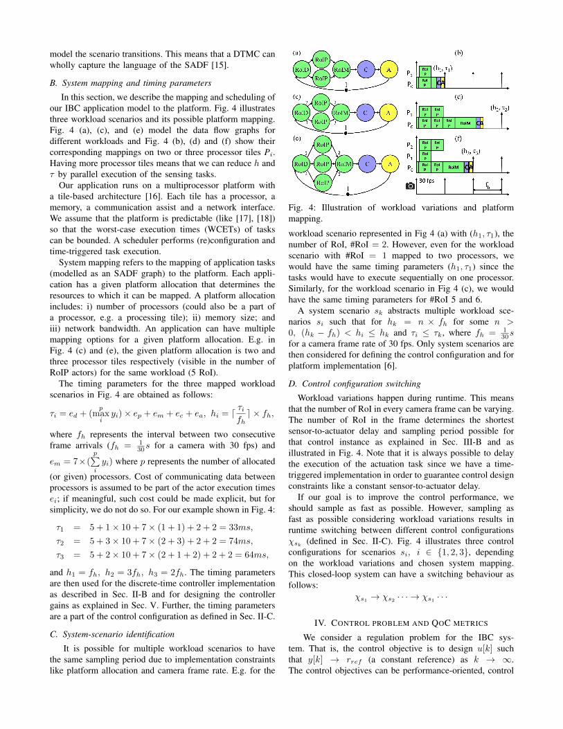
In this section, we describe the mapping and scheduling ofour IBC application model to the platform. Fig. 4 illustratesthree workload scenarios and its possible platform mapping.Fig. 4 (a), (c), and (e) model the data flow graphs fordifferent workloads and Fig. 4 (b), (d) and (f) show theircorresponding mappings on two or three processor tiles Pi.Having more processor tiles means that we can reduce h andτ by parallel execution of the sensing tasks.

Our application runs on a multiprocessor platform witha tile-based architecture [16]. Each tile has a processor, amemory, a communication assist and a network interface.We assume that the platform is predictable (like [17], [18])so that the worst-case execution times (WCETs) of taskscan be bounded. A scheduler performs (re)configuration andtime-triggered task execution.

System mapping refers to the mapping of application tasks(modelled as an SADF graph) to the platform. Each appli-cation has a given platform allocation that determines theresources to which it can be mapped. A platform allocationincludes: i) number of processors (could also be a part ofa processor, e.g. a processing tile); ii) memory size; andiii) network bandwidth. An application can have multiplemapping options for a given platform allocation. E.g. inFig. 4 (c) and (e), the given platform allocation is two andthree processor tiles respectively (visible in the number ofRoIP actors) for the same workload (5 RoI).

The timing parameters for the three mapped workloadscenarios in Fig. 4 are obtained as follows:

τi = ed + (p

maxiyi)× ep + em + ec + ea, hi = d τi

fhe × fh,

where fh represents the interval between two consecutiveframe arrivals (fh = 1

30s for a camera with 30 fps) and

em = 7×(p∑i

yi) where p represents the number of allocated

(or given) processors. Cost of communicating data betweenprocessors is assumed to be part of the actor execution timesei; if meaningful, such cost could be made explicit, but forsimplicity, we do not do so. For our example shown in Fig. 4:

τ1 = 5 + 1× 10 + 7× (1 + 1) + 2 + 2 = 33ms,

τ2 = 5 + 3× 10 + 7× (2 + 3) + 2 + 2 = 74ms,

τ3 = 5 + 2× 10 + 7× (2 + 1 + 2) + 2 + 2 = 64ms,

and h1 = fh, h2 = 3fh, h3 = 2fh. The timing parametersare then used for the discrete-time controller implementationas described in Sec. II-B and for designing the controllergains as explained in Sec. V. Further, the timing parametersare a part of the control configuration as defined in Sec. II-C.

C. System-scenario identification

It is possible for multiple workload scenarios to havethe same sampling period due to implementation constraintslike platform allocation and camera frame rate. E.g. for the

Fig. 4: Illustration of workload variations and platformmapping.

workload scenario represented in Fig 4 (a) with (h1, τ1), thenumber of RoI, #RoI = 2. However, even for the workloadscenario with #RoI = 1 mapped to two processors, wewould have the same timing parameters (h1, τ1) since thetasks would have to execute sequentially on one processor.Similarly, for the workload scenario in Fig 4 (c), we wouldhave the same timing parameters for #RoI 5 and 6.

A system scenario sk abstracts multiple workload sce-narios si such that for hk = n × fh for some n >0, (hk − fh) < hi ≤ hk and τi ≤ τk, where fh = 1

30sfor a camera frame rate of 30 fps. Only system scenarios arethen considered for defining the control configuration and forplatform implementation [6].

D. Control configuration switching

Workload variations happen during runtime. This meansthat the number of RoI in every camera frame can be varying.The number of RoI in the frame determines the shortestsensor-to-actuator delay and sampling period possible forthat control instance as explained in Sec. III-B and asillustrated in Fig. 4. Note that it is always possible to delaythe execution of the actuation task since we have a time-triggered implementation in order to guarantee control designconstraints like a constant sensor-to-actuator delay.

If our goal is to improve the control performance, weshould sample as fast as possible. However, sampling asfast as possible considering workload variations results inruntime switching between different control configurationsχsk (defined in Sec. II-C). Fig. 4 illustrates three controlconfigurations for scenarios si, i ∈ {1, 2, 3}, dependingon the workload variations and chosen system mapping.This closed-loop system can have a switching behaviour asfollows:

χs1 → χs2 · · · → χs1 · · ·

IV. CONTROL PROBLEM AND QOC METRICS

We consider a regulation problem for the IBC sys-tem. That is, the control objective is to design u[k] suchthat y[k] → rref (a constant reference) as k → ∞.The control objectives can be performance-oriented, control

effort/energy-oriented or a combination of both. The controlperformance quantifies, in essence, how fast the outputy[k] reaches the reference rref . The control effort is theamount of energy or power necessary for the controller toperform regulation. The control performance and effort areparameters that can be tuned in the cost function for theLQR design and MJLS synthesis using the state and inputweights. We evaluate QoC of an IBC application consideringthe following metrics: two commonly used control perfor-mance metrics - mean square error (MSE) and settling time(ST); and two commonly used metrics to evaluate controleffort/energy - power spectral density (PSD) and maximumcontrol effort (MCE).

A. Mean square error (MSE)

The MSE is the mean of the cumulative sum of the squarederrors, i.e.:

MSE =1

n

n∑k=1

(x[k]− rref )2

where n is the number of observations, x[k] is the value ofthe kth observation and rref is the reference value. A lowerMSE implies a better QoC.

B. Settling time (ST)

The settling time is defined as the time required for theoutput y[k] to reach and stay within a range of a certainpercentage (usually 5% or 2%) of the final (reference) valuerref for ever without external disturbances.

C. Power spectral density (PSD)

The PSD of a signal describes the power present in thesignal as a function of frequency, per unit frequency. It tellsus where the average power is distributed as a function offrequency. We use Welch’s overlapped segment averagingspectral estimation method [19] to compute PSD of ourcontrol input. Lower PSD for the control input signal impliesthat the energy required is less and hence QoC is better.

D. Maximum control effort (MCE)

We define the maximum control effort as maxk ‖u[k]‖. Alower MCE means better QoC. MCE can also be used toidentify input saturation, if any.

V. CONTROL DESIGN

The control design technique we choose decides thecontroller feedback and feedforward gains F and Ff for thecontrol law defined in Sec. II-C. To design a controller weassume that the sampling period hk and sensor-to-actuatordelay τk are known.

A. MJLS synthesis

In this section, we characterise the workload variationsas a discrete-time Markov chain (DTMC). The states of aDTMC model the workload scenarios and the transitionsmodel the scenario switching. We aggregate workload sce-narios into system scenarios as explained in Sec. III-C, andthen recompute transition and steady-state probabilities forthe DTMC. This results in a DTMC with number of statesequal to the number of identified system scenarios, witheach state representing a system scenario. We assume thatthe switching between the different control configurations isgoverned by this DTMC and show how the system in (II.1)can be re-cast as a Markov jump linear system (MJLS) [10].A Markov chain consists of a tuple M = (X,P ) where Xrepresents the state space, and P represents the one-step tran-sition probability matrix. In our context of system scenariosannotated with sampling period and sensor-to-actuator delay,the state-space of M is given by X = {s1, s2, s3}, wheresi = (hi, τi), i ∈ {1, 2, 3}, and

P =

p11 p12 p13p21 p22 p23p31 p32 p33

.Associated with M is a discrete-time stochastic process θ :N → X such that for all times sampling instances k ∈ N,and states si, sj ∈ X , i, j ∈ {1, 2, 3}, one has:

Prob(θ[k + 1] = sj | θ[k] = si) = pij ,

i.e. pij represents the probability of transitioning from statesi to sj . We assume that the initial condition of the stochasticprocess i.e. θ[0] is deterministic. The states here represent thesystem scenarios and the transitions represent the switchingbetween system scenarios based on the workload variations.For the sake of simplicity, we illustrate the formulation usingonly three states in the DTMC representing three systemscenarios. Note, however, that it is applicable to any numberof identified system scenarios (as explained in Sec. III-C).

Using a zero order sample-and-hold approach, it can bereadily shown that Eq. (II.1) can be re-formulated intoan MJLS governed by the following stochastic differenceequations:

x[k + 1] = Aθ[k]x[k] +B0,θ[k]u[k] +B1,θ[k]u[k − 1],

y[k] = Ccx[k] (V.1)

where for each si ∈ X , i ∈ {1, 2, 3}: Asi , B0,si , and B1,si

are computed using Eq. (II.3). In Eq.(V.1) we assume thatu[−1] = 0 for k = 0. We define the new system statesz[k] =

[x[k] u[k − 1]

]Twith z[0] =

[x[0] 0

]Tto obtain

a higher-order augmented system as follows:

z[k + 1] = Aaug,θ[k]z[k] +Baug,θ[k]u[k],

yz[k] = Caugz[k]

where for each si ∈ X, i ∈ {1, 2, 3}: Aaug,si and Baug,siare computed using Eq. (II.5) and Caug =

[Cc 0

].

Infinite horizon quadratic optimal controller: Here, wepresent the control law design for the MJLS (V.1). We designa controller to minimize the infinite horizon cost given by

J(θ[0], z[0], u[0]) =

∞∑k=0

E[z[k]TCTaugCaugz[k] + d2u|u[k]|2],

where du ∈ R>0 represents the input weight and the notationE[X] represents the expected value of a random variable X .

It is shown in [10] that the solution to the above infinitehorizon optimal control problem can be obtained by solvingthe coupled algebraic Riccati (matrix) equations (CARE)

Γi = ATaug,siEi(Γ)Aaug,si + CTc Cc

−ATaug,siEi(Γ)Baug,si(BTaug,siEiBaug,si)

−1BTaug,siEi(Γ)Aaug,si

where Ei(Γ) =

3∑j=0

pijΓj

where i ∈ {1, 2, 3} and Γ = {Γ1,Γ2,Γ3} are the unknownmatrices to be solved for. The mean-square stabilizing opti-mal control law is then given by

u[k] = Fθ[k](Γ)x[k] + Ff,θ[k]rref ,

where

Fsi = −(BTaug,siEi(Γ)Baug,si)−1BTaug,siEi(Γ)Aaug,si ,

Ff,si =1

Caug(I − (Aaug,si − FsiBaug,si))−1Baug,si,

where i ∈ {1, 2, 3}. It is shown in Theorem A.12 in [10]the above CARE can be solved by solving a related convexoptimization problem, the details of which are omitted dueto lack of space.

B. LQR design with worst-case workload

We consider the system scenario for the worst-case work-load swc having the worst-case period and delay (hwc, τwc)(one of the scenarios as explained in Sec. III-C) for designingthe control law. We design a controller to minimize thefollowing cost function

J(u) =

∞∑k=0

z[k]T dsCTaugCaugz[k] + d2u|u[k]|2,

where du, ds ∈ R>0 represents the input weight and thestate weights respectively. The weights are optimized for theconsidered QoC metric. Typically, du � ds so as to optimisefor control performance and du � ds to optimise for controlenergy (see Sec. VI-B).

C. Switched linear control design

The switched linear control design we consider is ex-plained in [6]. Frequently occurring workload scenarios arecharacterised using the the PERT distribution. A set ofoptimal system scenarios are identified. LQR controllers aredesigned for each of these scenarios si with (hi, τi) thatminimises the cost function given in Sec. V-B. Further, thestability of this switched system is analysed by derivinglinear matrix inequalities (LMIs) that check for the existenceof a common quadratic Lyapunov function (CQLF).

VI. RESULTS, OBSERVATIONS AND GUIDELINES

We consider the case-study of vision-based lateral controlfor a vehicle (explained in Sec. II) for comparison of thethree approaches for control design with respect to theQoC metrics described earlier. The controllers for LQR andswitched linear control are tuned for the corresponding QoCmetric evaluation by adjusting the input and state weights.

A. Simulation setup

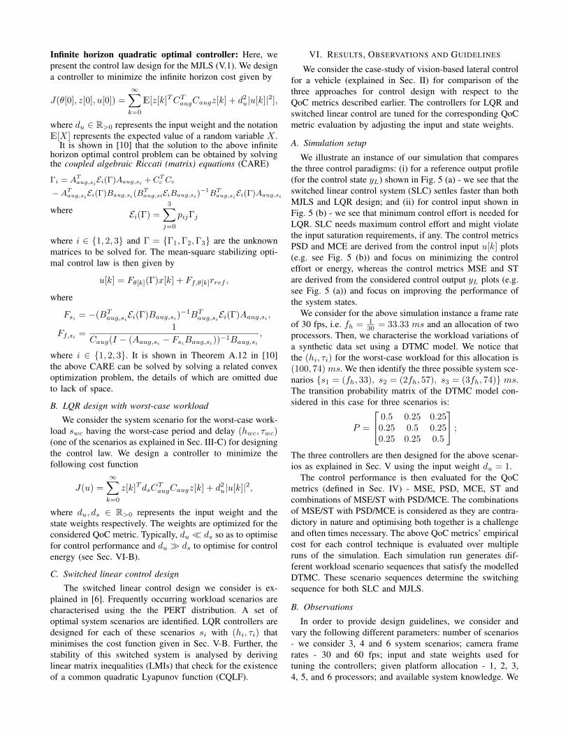
We illustrate an instance of our simulation that comparesthe three control paradigms: (i) for a reference output profile(for the control state yL) shown in Fig. 5 (a) - we see that theswitched linear control system (SLC) settles faster than bothMJLS and LQR design; and (ii) for control input shown inFig. 5 (b) - we see that minimum control effort is needed forLQR. SLC needs maximum control effort and might violatethe input saturation requirements, if any. The control metricsPSD and MCE are derived from the control input u[k] plots(e.g. see Fig. 5 (b)) and focus on minimizing the controleffort or energy, whereas the control metrics MSE and STare derived from the considered control output yL plots (e.g.see Fig. 5 (a)) and focus on improving the performance ofthe system states.

We consider for the above simulation instance a frame rateof 30 fps, i.e. fh = 1

30 = 33.33 ms and an allocation of twoprocessors. Then, we characterise the workload variations ofa synthetic data set using a DTMC model. We notice thatthe (hi, τi) for the worst-case workload for this allocation is(100, 74) ms. We then identify the three possible system sce-narios {s1 = (fh, 33), s2 = (2fh, 57), s3 = (3fh, 74)} ms.The transition probability matrix of the DTMC model con-sidered in this case for three scenarios is:

P =

0.5 0.25 0.250.25 0.5 0.250.25 0.25 0.5

;

The three controllers are then designed for the above scenar-ios as explained in Sec. V using the input weight du = 1.

The control performance is then evaluated for the QoCmetrics (defined in Sec. IV) - MSE, PSD, MCE, ST andcombinations of MSE/ST with PSD/MCE. The combinationsof MSE/ST with PSD/MCE is considered as they are contra-dictory in nature and optimising both together is a challengeand often times necessary. The above QoC metrics’ empiricalcost for each control technique is evaluated over multipleruns of the simulation. Each simulation run generates dif-ferent workload scenario sequences that satisfy the modelledDTMC. These scenario sequences determine the switchingsequence for both SLC and MJLS.

B. Observations

In order to provide design guidelines, we consider andvary the following different parameters: number of scenarios- we consider 3, 4 and 6 system scenarios; camera framerates - 30 and 60 fps; input and state weights used fortuning the controllers; given platform allocation - 1, 2, 3,4, 5, and 6 processors; and available system knowledge. We

0 5 10 15

time (s)

-0.04

-0.03

0

0.03

0.04

yL (

m)

SLCMJLS

LQRReference

(a) Output yL when input weight du = 1.

0 5 10 15

time (s)

-8

-4

0

4

8

u(t

)

10-3

SLC

MJLS

LQR

(b) Input u[k] when input weight du = 1.

0 5 10 15

time (s)

-0.04

-0.03

0

0.03

0.04

yL (

m)

SLCMJLS

LQRReference

(c) Output yL when input weight du = 10.

0 5 10 15

time (s)

-3

-2

-1

0

1

2

3

u(t

)

10-3

SLC

MJLS

LQR

(d) Input u[k] when input weight du = 10.

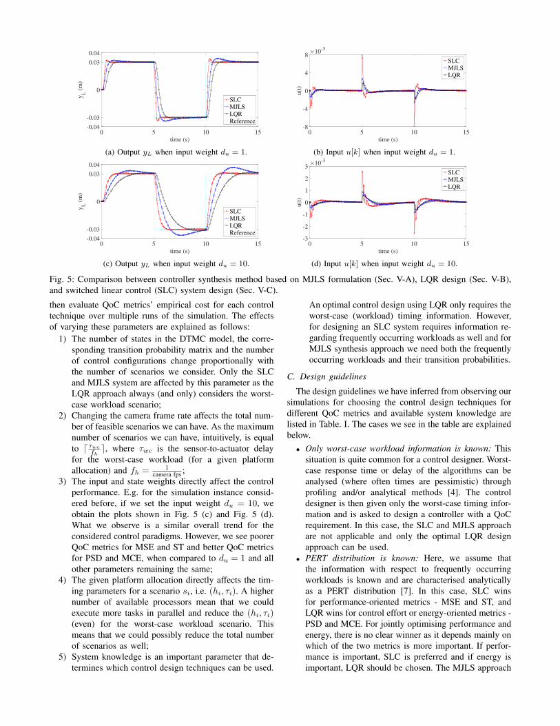
Fig. 5: Comparison between controller synthesis method based on MJLS formulation (Sec. V-A), LQR design (Sec. V-B),and switched linear control (SLC) system design (Sec. V-C).

then evaluate QoC metrics’ empirical cost for each controltechnique over multiple runs of the simulation. The effectsof varying these parameters are explained as follows:

1) The number of states in the DTMC model, the corre-sponding transition probability matrix and the numberof control configurations change proportionally withthe number of scenarios we consider. Only the SLCand MJLS system are affected by this parameter as theLQR approach always (and only) considers the worst-case workload scenario;

2) Changing the camera frame rate affects the total num-ber of feasible scenarios we can have. As the maximumnumber of scenarios we can have, intuitively, is equalto d τwc

fhe, where τwc is the sensor-to-actuator delay

for the worst-case workload (for a given platformallocation) and fh = 1

camera fps ;3) The input and state weights directly affect the control

performance. E.g. for the simulation instance consid-ered before, if we set the input weight du = 10, weobtain the plots shown in Fig. 5 (c) and Fig. 5 (d).What we observe is a similar overall trend for theconsidered control paradigms. However, we see poorerQoC metrics for MSE and ST and better QoC metricsfor PSD and MCE, when compared to du = 1 and allother parameters remaining the same;

4) The given platform allocation directly affects the tim-ing parameters for a scenario si, i.e. (hi, τi). A highernumber of available processors mean that we couldexecute more tasks in parallel and reduce the (hi, τi)(even) for the worst-case workload scenario. Thismeans that we could possibly reduce the total numberof scenarios as well;

5) System knowledge is an important parameter that de-termines which control design techniques can be used.

An optimal control design using LQR only requires theworst-case (workload) timing information. However,for designing an SLC system requires information re-garding frequently occurring workloads as well and forMJLS synthesis approach we need both the frequentlyoccurring workloads and their transition probabilities.

C. Design guidelines

The design guidelines we have inferred from observing oursimulations for choosing the control design techniques fordifferent QoC metrics and available system knowledge arelisted in Table. I. The cases we see in the table are explainedbelow.• Only worst-case workload information is known: This

situation is quite common for a control designer. Worst-case response time or delay of the algorithms can beanalysed (where often times are pessimistic) throughprofiling and/or analytical methods [4]. The controldesigner is then given only the worst-case timing infor-mation and is asked to design a controller with a QoCrequirement. In this case, the SLC and MJLS approachare not applicable and only the optimal LQR designapproach can be used.

• PERT distribution is known: Here, we assume thatthe information with respect to frequently occurringworkloads is known and are characterised analyticallyas a PERT distribution [7]. In this case, SLC winsfor performance-oriented metrics - MSE and ST, andLQR wins for control effort or energy-oriented metrics -PSD and MCE. For jointly optimising performance andenergy, there is no clear winner as it depends mainly onwhich of the two metrics is more important. If perfor-mance is important, SLC is preferred and if energy isimportant, LQR should be chosen. The MJLS approach

TABLE I: Guidelines for choosing the control design techniques: MJS (Sec. V-A), LQR (Sec. V-B), SLC (Sec. V-C).

Available system knowledgeQoC metrics

Performance Control energy Performanceand EnergyMSE ST MCE PSD

Only worst-case workload information LQR LQR LQR LQR LQRFrequently occurring workloads as a PERT SLC SLC LQR LQR SLC/ LQRFrequently occurring workloads and their

transition probabilities as a DTMCSLC/MJS

SLC/MJS

MJS/LQR

MJS/LQR MJS

is not applicable as more information is needed.• DTMC model is known: Information regarding fre-

quently occurring workloads and their transition proba-bilities are needed for modelling a DTMC. These can beestimated from observed workload variations data [8].Intuitively, this means that we can predict the possible(workload) scenario switching sequences for the controldesign. However, for the above two cases the switchingsequence is assumed to be arbitrary and not known. Inthis case, for performance metrics, MJLS wins whenthe input weight du is very small (since SLC tends tooscillate before settling). However, for a large value ofdu, there is no clear winner between SLC and MJLS andit depends on the application and chosen parameters.Please note, however, that a challenge of SLC is to provethe stability of the designed system. MJLS is a synthesismethod and the design, if any, is stable by construction.If we consider control effort or energy metrics, LQRwins when the input weight du is small and there isno clear winner between LQR and MJLS for a largeinput weight du as the results are similar and dependson the application and chosen parameters. MJLS is theclear winner if we consider a joint optimisation forperformance and energy QoC metrics.

VII. CONCLUSION

We present a MJLS formulation for controller synthesisfor image-based control systems considering workload vari-ations and platform implementation constraints. Further, wecompare our method with two relevant control paradigms:LQR and switched linear control system design. We alsoprovide design guidelines on the control technique to usefor given constraints on the system knowledge, the QoC andthe implementation.

The synthesis method assumes that the workload varia-tions can be characterised as a DTMC. A DTMC is sensitiveto the data used for its modelling. As a future work,sensitivity analysis of the DTMC towards the QoC needsto be evaluated. Further, the current design guidelines areprovided based on multiple empirical simulation runs ofthe controller for varying workloads, number of scenarios,camera frame rate and given platform allocation. A formalmathematical analysis would strengthen our design guide-lines and is planned as future work. The challenge for aformal analysis of the control design is that we do not knowthe exact sequence of occurrence of the workload variationsapriori.

REFERENCES

[1] P. Corke, Robotics, Vision and Control: Fundamental Algorithms InMATLAB R© Second, Completely Revised. Springer, 2017, vol. 118.

[2] E. van Horssen, “Data-intensive feedback control: switched systemsanalysis and design,” Ph.D. dissertation, Eindhoven University ofTechnology, 2018.

[3] S. D. Pendleton, H. Andersen, X. Du, X. Shen, M. Meghjani, Y. H.Eng, D. Rus, and M. H. Ang, “Perception, planning, control, andcoordination for autonomous vehicles,” Machines, vol. 5, no. 1, p. 6,2017.

[4] S. Saidi, S. Steinhorst, A. Hamann, D. Ziegenbein, and M. Wolf, “Fu-ture automotive systems design: research challenges and opportunities:special session,” in Proceedings of the International Conference onHardware/Software Codesign and System Synthesis, 2018.

[5] R. C. Dorf and R. H. Bishop, Modern control systems. Pearson, 2011.[6] S. Mohamed, D. Zhu, D. Goswami, and T. Basten, “Optimising

quality-of-control for data-intensive multiprocessor image-based con-trol systems considering workload variations,” in 21st EuromicroConference on Digital System Design (DSD), 2018, pp. 320–327.

[7] S. Adyanthaya, Z. Zhang, M. Geilen, J. Voeten, T. Basten, andR. Schiffelers, “Robustness analysis of multiprocessor schedules,” inInternational Conference on Embedded Computer Systems: Architec-tures, Modeling, and Simulation (SAMOS), 2014, pp. 9–17.

[8] N. J. Welton and A. Ades, “Estimation of markov chain transi-tion probabilities and rates from fully and partially observed data:uncertainty propagation, evidence synthesis, and model calibration,”Medical Decision Making, vol. 25, no. 6, pp. 633–645, 2005.

[9] J. Kosecka, R. Blasi, C. Taylor, and J. Malik, “Vision-based lateralcontrol of vehicles,” in Proceedings of Conference on IntelligentTransportation Systems. IEEE, 1997, pp. 900–905.

[10] O. L. V. Costa, M. D. Fragoso, and R. P. Marques, Discrete-timeMarkov jump linear systems. Springer, 2006.

[11] K. Ogata et al., Discrete-time control systems. Prentice Hall Engle-wood Cliffs, NJ, 1995, vol. 2.

[12] G. Goodwin, P. Ramadge, and P. Caines, “Discrete-time multivariableadaptive control,” IEEE Transactions on Automatic Control, vol. 25,no. 3, pp. 449–456, 1980.

[13] A. Bemporad, F. Borrelli, M. Morari et al., “Model predictive controlbased on linear programming-the explicit solution,” IEEE transactionson automatic control, vol. 47, no. 12, pp. 1974–1985, 2002.

[14] H. Alizadeh Ara, A. Behrouzian, M. Hendriks, M. Geilen,D. Goswami, and T. Basten, “Scalable analysis for multi-scaledataflow models,” ACM Transactions on Embedded Computing Sys-tems (TECS), vol. 17, no. 4, p. 80, 2018.

[15] B. D. Theelen, M. Geilen, T. Basten, J. Voeten, S. V. Gheorghita, andS. Stuijk, “A scenario-aware data flow model for combined long-runaverage and worst-case performance analysis,” in Formal Methods andModels for Co-Design (MEMOCODE), 2006, pp. 185–194.

[16] S. Stuijk, “Predictable mapping of streaming applications on multi-processors,” Ph.D. dissertation, Eindhoven University of Technology,2007.

[17] A. Hansson, K. Goossens, M. Bekooij, and J. Huisken, “CoMPSoC:A template for composable and predictable multi-processor system onchips,” ACM Transactions on Design Automation of Electronic Systems(TODAES), vol. 14, no. 1, p. 2, 2009.

[18] S. A. Edwards and E. A. Lee, “The case for the precision timed(PRET) machine,” in Design Automation Conference (DAC). IEEE,2007, pp. 264–265.

[19] P. Welch, “The use of FFT for the estimation of power spectra: amethod based on time averaging over short, modified periodograms,”IEEE Trans. on audio & electroacoustics, vol. 15, no. 2, pp. 70–73,1967.