Designing efficient resource sharing for impatient players using limited monitoring

Designing Efficient Resource Sharing For Impatient Players

Using Limited MonitoringI

Mihaela van der Schaara, Yuanzhang Xiaob, William Zamec

aDepartment of Electrical Engineering, UCLA. Email: [email protected] of Electrical Engineering, UCLA. Email: [email protected].

cCorresponding Author Department of Economics, UCLA, Los Angeles, CA 90095Email: [email protected]; Telephone 310-985-3091

Abstract

The problem of efficient sharing of a resource is nearly ubiquitous. Exceptfor pure public goods, each agent’s use creates a negative externality; oftenthe negative externality is so strong that efficient sharing is impossible inthe short run. We show that, paradoxically, the impossibility of efficientsharing in the short run enhances the possibility of efficient sharing in thelong run, even if outcomes depend stochastically on actions, monitoring islimited and users are not patient. We base our analysis on the familiar frame-work of repeated games with imperfect public monitoring, but we extend theframework to view the monitoring structure as chosen by a designer whobalances the benefits and costs of more accurate observations and reports.Our conclusions are much stronger than in the usual folk theorems: we donot require a rich signal structure or patient users and provide an explicitonline construction of equilibrium strategies.

Keywords: repeated games, imperfect public monitoring, perfect publicequilibrium, efficient outcomes, resource allocation games

JEL: C72, C73, D02

IThis research was supported by National Science Foundation (NSF) Grants No.0830556, (van der Schaar, Xiao) and 0617027 (Zame) and by the Einaudi Institute forEconomics and Finance (Zame). Any opinions, findings, and conclusions or recommenda-tions expressed in this material are those of the authors and do not necessarily reflect theviews of any funding agency.

Preprint submitted to Elsevier September 1, 2013

1. Introduction

The problem of efficient sharing of a resource – a physical resource, a

prize, a market – is nearly ubiquitous. Unless the resource is a pure public

good, each agent’s use of the resource imposes a negative externality on other

users. Hence (self-interested, strategic) agents will find it difficult to share the

resource efficiently, at least in the short run. In some circumstances – those

we focus on in this paper – the negative externality is so strong – competition

for the resource is so destructive – that it will be impossible for users so share

the resource efficiently, at least in the short run. The purpose of this paper is

to show that – perhaps paradoxically – the impossibility of efficient sharing

in the short run enhances the possibility of efficient sharing in the long run

– even when outcomes depend stochastically on actions, monitoring is very

limited and players are not very patient.

We formalize our analysis using the familiar framework of repeated games

with imperfect public monitoring but with important differences in both the

formulation and the conclusions. With respect to the formulation, the impor-

tant difference is in the way we view the monitoring structure. In the usual

models of games with imperfect public monitoring, the monitoring struc-

ture is viewed as exogenous and fixed. In the canonical model of Green and

Porter (1984) for instance, the players compete in a Cournot quantity-setting

game but receive feedback only about market prices (rather than quantity

choices of other firms) which are determined by random market demand.

We are motivated by the many situations in which the feedback received by

the players arises from the action choices of a strategic actor – the designer

–who must weigh (among other considerations) the trade-offs between more

1

accurate observations of player actions and more accurate reports provided

to players about those observations on the one hand and the costs and conse-

quences of observations and reports on the other hand. Consider for instance

a repeated contest (for details see Example 2 in Section 3). In each period,

players choose effort levels which determine (stochastically) the contest win-

ner. The designer (in this case the contest operator) does not observe effort

– and so certainly cannot announce it – but does observe the identity of the

winner, and could announce that. However announcing the identify of the

winner would violate the privacy of the winner and the losers; if privacy is

valued, the designer must weigh the trade-off between the value of maintain-

ing privacy and the (possible) efficiency gain of making more information

public. Because we wish to emphasize the role played by this and similar

choices of the monitoring structure we formalize an elaborated model in

which the choice of the monitoring structure – both what the designer ob-

serves and what the designer announces – is made explicit. However, the

reduced form that results from our elaborated model once the designer has

chosen a monitoring structure looks just the same as the reduced form that

is familiar from the standard model of repeated games with imperfect public

monitoring.

With respect to conclusions, we cite three important differences: we do

not assume a rich signal structure (rather, we require only two signals), we do

not assume players are arbitrarily patient (rather, we find an explicit lower

bound on the requisite discount factor), and we provide an explicit (dis-

tributed) algorithm that takes as inputs the parameters – stage game payoffs,

discount factor, target payoff – and computes the strategy – the action to be

2

chosen by each player following each public history. This algorithm can be

carried out by each player separately and in real time – there is no need for

the designer to specify/describe the strategies to be played. A consequence

of our constructive algorithm is that the strategies we identify enjoy a use-

ful robustness property: generically, the equilibrium strategies are, for many

periods, locally constant in the parameters of the environment and of the

problem.

Within our structure, we abstract what we see as the essential features of

the resource allocation problems by two assumptions about the stage game.

The first is that for each player i there is a unique action profile ai that i

most prefers. (In the resource allocation scenario, ai would be the profile

in which only player i accesses the resource.) The second is that for every

action profile a that is not in the set ai of preferred action profiles the

corresponding utility profile U(a) lies below the hyperplane H spanned by

the utility profiles U(ai). (In the resource allocation scenario, this corre-

sponds to the assumption that allowing access to the resource by more than

one individual strictly lowers (weighted) social welfare.) We capture the no-

tion that monitoring is very limited by assuming that players do not observe

the profile a of actions but rather only some signal y ∈ Y whose distribution

ρ(y|a) depends on the true profile a, and that (profitable) single-player de-

viations from i’s preferred action profile ai can be statistically distinguished

from conformity with ai in the same way. (But we do not assume that dif-

ferent deviations from ai can be distinguished from from each other. For

further comments, see Examples 2 and 3 in Section 3.) We emphasize the

setting in which there are only two signals – “good” and “bad” – because

3

this setting offers the sharpest results and the clearest intuition and, as we

shall see, because two signals are often enough. To help understand the com-

monplace nature of our problem and assumptions, we offer three examples:

the first is a repeated prisoner’s dilemma (although with lower cooperative

payoffs than usual), the second is a repeated contest, the third is a repeated

resource sharing game.

Not surprisingly we build on the framework of (Abreu, Pearce, and Stac-

chetti (1990); hereafter APS). Our main technical result (Theorem 1) pro-

vides conditions (on the information and payoff structures and the discount

factor) that are both necessary and sufficient for the set of payoffs that guar-

antee each player a given level of security to be self-generating. Because

every payoff vector in a self-generating set can be supported in a perfect

public equilibrium (PPE), this leads immediately to sufficient conditions for

the same sets to consist of payoff vectors that can be achieved in PPE, and an

algorithm for the corresponding PPE strategies (Theorem 2). Our robustness

conclusion (Theorem 3) follows from the nature of the algorithm. For games

with two players, other considerations lead to the conclusion that maximal

sets of PPE payoffs must have a special form and so thus to a characteriza-

tion of the maximal set of PPE payoffs (Theorem 4). A surprising aspect of

this characterization is that there is a discount factor δ∗ < 1 such that any

efficient payoff that can be achieved as a PPE payoff for some discount factor

δ can already be achieved as a PPE payoff as soon as the discount factor δ

exceeds some threshold δ∗. Patience is rewarded – but only up to a point.1

1Mailath, Obara, and Sekiguchi (2002) establish a similar result for the repeated Pris-oner’s Dilemma with perfect monitoring; Athey and Bagwell (2001) establish a parallel

4

The literature on repeated games with imperfect public monitoring is

quite large – much too large to survey here; we refer instead to Mailath and

Samuelson (2006) and the references therein. However, explicit comparisons

with two papers in this literature may be especially helpful. The first and

most obvious comparison is with (Fudenberg, Levine, and Maskin (1994);

hereafter FLM) on the Folk Theorem for repeated games with imperfect

public monitoring. As do we, FLM consider a situation in which a single

stage game G with action space A and utility function U : A → Rn is played

repeatedly over an infinite horizon; monitoring is public but imperfect, so

players do not observe actions but only a public signal of those actions. In

this setting, co[U(A)] is the closure of the set of payoff profiles that can be

achieved as long run average utilities for some discount factor and some infi-

nite set of plays of the stage game G. Under certain assumptions, FLM prove

that any payoff vector in the interior of co[U(A)] that is strictly individually

rational can be achieved in a PPE of the infinitely repeated game. However,

the assumptions FLM maintain are very different from ours in two very im-

portant dimensions (and some other dimensions that seem less important,

at least for the present discussion). The first is that the signal structure

is rich and informative; in particular, that the number of signals is at least

one less than the number of actions of any two players. The second is that

players are arbitrarily patient: that is, the discount factor δ is as close to

1 as we like. (More precisely: given a target utility profile v, there is some

δ(v) such that if the discount factor δ > δ(v) then there is a PPE of the

result for symmetric equilibrium payoffs of two-player symmetric repeated Bertrand games.We are unaware of any general results that have this flavor.

5

repeated game that yields the target utility profile v.) In particular, FLM

do not identify any PPE for any given discount factor δ < 1. By contrast,

we require only two signals even if action spaces are infinite and we do not

assume players are patient: all target payoffs can be achieved for some fixed

discount factor – which may be very far from 1. Moreover, because FLM

consider only payoffs in the interior of co[U(A)], they have nothing to say

about achieving efficient payoffs. Their results do imply that efficient pay-

offs can be arbitrarily well approximated by payoffs that can be achieved in

PPE, but only if the corresponding discount factors are arbitrarily close to

1. By contrast, (Fudenberg, Levine, and Takahashi (2007); hereafter FLT)

do show how (some) efficient payoffs can be achieved in PPE. Given Pareto

weights λ1, . . . , λn set Λ = sup∑λiUi(a) : a ∈ A and consider the hyper-

plane H = x ∈ Rn :∑λixi = Λ. The intersection H ∩ co[U(A)] is a part

of the Pareto boundary of co[U(A)]. As do we, FLT ask what vectors in

H ∩ co[U(A)] can be achieved in PPE of the infinitely repeated game. They

identify the largest (compact convex) set Q ⊂ H ∩ co[U(A)] with the prop-

erty that every target vector v ∈ intQ (the relative interior of Q with respect

to H) can be achieved in a PPE of the infinitely repeated game for some

discount factor δ(v) < 1. However, because FLT consider arbitrary stage

games and arbitrary monitoring structures, the set Q identified by FLT may

be empty, and FLT do not provide any conditions that guarantee that Q is

not empty. Moreover, as in FLM, FLT assume that players are arbitrarily

patient, so do not identify any PPE for any given discount factor δ < 1. Hav-

ing said this, we should also point out that FLT identify the closure of the

set of all payoff vectors in the interior of H ∩ co[U(A)] that can be achieved

6

in a PPE for some discount factor, while we identify only some. So there is

a trade-off: FLT find more PPE payoffs but provide much less information

about the ones they find; we find fewer PPE payoffs but provide much more

information about the ones we find.

At the risk of repetition, we want to emphasize the most important fea-

tures of our results. The first is that we do not assume discount factors are

arbitrarily close to 1. The importance of this seems obvious in all environ-

ments – especially since the discount factor encodes both the innate patience

of players and the probability that the interaction continues. The second

is that we impose different – and in many ways weaker – requirements on

the monitoring structure; indeed, we require only two signals, even if action

spaces are infinite. Again, the importance of this seems obvious in all envi-

ronments, but especially in those in which signals are not generated by some

exogenous process but must be provided by a designer. In the latter case it

seems obvious – and in practice may be of supreme importance – that the

designer may wish or need to choose a simple information structure that em-

ploys a small number of signals, saving on the cost of observing the outcome

of play and on the cost of communicating to the agents (and preserving pri-

vacy as well). More generally, the designer may face a trade-off between the

efficiency obtainable with a finer information structure and the cost of using

that information structure. (We will return to this point later.) Finally,

because we provide a distributed algorithm for calculating equilibrium play,

neither the agents nor a designer need to work out the equilibrium strategies

in advance; all calculations can be done online, in real time.

Following this Introduction, Section 2 presents the formal model; Section

7

3 presents three examples that illustrate the model. Section 4 presents some

preliminary results, presenting conditions under which no efficient payoffs

can be achieved in PPE for any discount factor. Section 5 presents the main

technical result (Theorem 1); Section 6 presents the implications for PPE

(Theorems 2,3) and a comparison with FLT; Section 7 specializes to the case

of two players (Theorem 4). Section 8 returns to the examples to illustrate

both the conclusions and the general framework. Section 9 concludes. We

relegate all proofs to the Appendix.

2. Model

The reduced form of our model will closely resemble the familiar frame-

work of a repeated game with imperfect public monitoring and we state and

prove our formal results in the context of that reduced form. However, be-

cause we want to emphasize the role played by the designer, we begin by

presenting a more elaborated form.

2.1. Stage Game: Elaborated Form

There are n + 1 (potential) actors in our framework: n players and a

designer. Players are characterized by an (exogenously given) game form:

• a (measurable) space Z of outcomes

• for each player i

– a (measurable) space Ai of actions

– a (measurable) utility function ui : Ai × Z → R

• a (measurable) mapping a 7→ π(·|a) : A = A1 × · · · × An → ∆(Z)

8

We view π(z|a) as the probability that the outcome z ∈ Z occurs when

players choose the action profile a ∈ A. Thus the joint actions of players

a ∈ A stochastically determine an outcome z ∈ Z, and each player’s realized

utility depends on its own action and the realized outcome.2 For the moment

we require only that the spaces Ai, the utility functions ui and the probability

mapping π be measurable, so that utilities in the reduced form be defined;

but later we will insist that the spaces be compact metric and that the utility

functions and the probability mapping be continuous.

The designer is characterized by a monitoring technology:

• a set of Φ of pairs (X,ϕ) where:

– X is a (measurable) space

– z 7→ ϕ(·|z) : Z → ∆(X) is a (measurable) mapping

A pair (X,ϕ) is a measurement device.

• a set Ψ of pairs (Y, ψ) where

– Y is a (measurable) space

– x 7→ ψ(·|x) : X → ∆(Y ) is a (measurable) mapping

A pair (Y, ψ) is an announcement rule.

For the moment, we again require only that the spacesX,Y and the mappings

ϕ, ψ be measurable, but later we will insist that the spaces be compact metric

and that the mappings be continuous. Given a choice (X,ϕ) ∈ Φ we interpret

2We could incorporate actions into the space Z of outcomes so that realized utilitydepended only on outcomes, but it seems useful to keep separate track of own actions.

9

ϕ(x|z) as the probability that the designer measures (observes) x when the

outcome z has actually occurred. Given a choice (Y, ψ) ∈ Ψ, we interpret

ψ(y|x) as the probability that the designer makes the (public) announcement

of the signal y ∈ Y when the observation x has actually been made. A pair

of choices (X,ϕ) ∈ Φ, (Y, ψ) ∈ Ψ constitute the monitoring structure.

2.2. Stage Game: Reduced Form

The reduced form of the stage game consists of

• a set N = 1, . . . , n of players

• for each player i

– a (measurable) space Ai of actions

– a (measurable) utility function Ui : A = A1 × · · · × An → R

• a (measurable) compact metric space of public signals Y

• a (measurable) map a 7→ ρ(·|a) : A → ∆(Y )

We interpret Ui(a) as i’s ex ante (expected) utility when a is played and

ρ(y|a) as the probability that the signal y is observed when a is played.

2.3. Stage Game: From the Elaborated Form to the Reduced Form

To pass from the elaborated form to the reduced form we simply define

the ex ante (expected) utilities Ui(a) and and the probability distribution

ρ(·|a) over public signals as functions of the action profile a that is played.

10

For a ∈ A and D ⊂ Y these are:

Ui(a) =∫

Zui(ai, z) dπ(z|a)

ρ(D|a) =∫

Y

∫X

∫Z1D dψ(y|x) dϕ(x|z) dπ(z|a)

If Z,X, Y are all finite the last equation can be re-written more simply as

ρ(y|a) =∑x∈X

∑z∈Z

ψ(y|x)ϕ(x|z)π(z|a)

Under the maintained assumptions on realized utility, outcome mapping,

measurement technology and announcement rules, the derived ex ante utili-

ties and signal distribution are measurable; if the former are continuous, so

are the latter.

2.4. The Repeated Game with Imperfect Public Monitoring

In the repeated game, the reduced stage game G is played in every period

t = 0, 1, 2, . . .. Given the signal structure, a public history of length t is a

sequence (y0, y1, . . . , yt−1) ∈ Y t. We write H(t) for the set of public histories

of length t, HT =⋃T

t=0H(t) for the set of public histories of length at most

T and H =⋃∞

t=0H(t) for the set of all public histories of all finite lengths. A

private history for player i includes the public history, the actions taken by

player i, and the realized utilities observed by player i, so a private history of

length t is a a sequence (a0i , . . . , a

t−1i ;u0

i , . . . , ut−1i ; y0, . . . , yt−1) ∈ At

i×Rt×Y t.

We write Hi(t) for the set of i’s private histories of length t, HTi =

⋃Tt=0Hi(t)

for the set of i’s private histories of length at most T and Hi =⋃∞

t=0Hi(t)

11

for the set of i’s private histories of all finite lengths.

A pure strategy for player i is a mapping from all private histories into

the set of pure actions σi : Hi → Ai. A public strategy for player i is a pure

strategy that is independent of i’s own action/utility history; equivalently, a

mapping from public histories to i’s pure actions σi : H → Ai.

We assume all players discount future utilities using the same discount

factor δ ∈ (0, 1) and we use long-run averages, so if the stream of expected

utilities is ut the vector of long-run average utilities is (1− δ)∑∞t=0 δ

tut. A

strategy profile σ : H1 × . . . × Hn → A induces a probability distribution

over public and private histories and hence over ex ante utilities. We abuse

notation and write U(σ) for the vector of expected (with respect to this dis-

tribution) long-run average ex ante utilities when players follow the strategy

profile σ.

As usual a strategy profile σ is an equilibrium if each player’s strategy

is optimal given the strategies of others. A strategy profile is a public equi-

librium if it is an equilibrium and each player uses a public strategy; it is a

perfect public equilibrium (PPE) if it is a public equilibrium following every

public history.

2.5. Interpretation

In our formulation, which restricts players to use public strategies, we

tacitly assume that players make no use of any information other than that

provided by the public signal; in particular, players make no use of infor-

mation that might be provided by the realized utility they experience each

period. As discussed in Mailath and Samuelson (2006), this assumption ad-

mits a number of possible interpretations, each of which is appropriate in

12

some circumstances. The first is that utility is not realized until the game

terminates. The second is that the outcome z and the public signal y coin-

cide, so that realized utility depends only on own action and the public signal

(both of which are observed). The third is that – at least in the equilibria and

deviations under consideration – the information provided by realized utility

is already provided by the public signal. (See Example 2 below.) A fourth

is that even if utility is realized during play and realized utility does provide

information not provided by the public signal, this additional information is

not used. Lest this last interpretation seems odd, recall that if players other

than i follow public strategies then it is optimal for player i to follow a pub-

lic strategy as well; in particular if other players make no use of information

provided by their own realized utility then it is optimal for player i to make

no use of information provided by i’s realized utility. (Again, see Example 2

below.) Finally, it should be kept in mind that by restricting our attention

to PPE we are tying our own hands; since our objective is to support efficient

sharing, restricting to a particular class of strategies only makes our results

stronger.

2.6. Assumptions on the Stage Game

To this point we have described a very general setting; we now impose

additional assumptions – first on the stage game and then on the information

structure – that we exploit in our results.

We assume that the spaces Z,Ai, X, Y are all compact metric and that

the functions/mappings ui, π, ϕ, ψ are all continuous; as noted this implies

that the functions/mappings Ui, ρ are continuous as well.

Set U(A) = U(a) ∈ Rn : a ∈ A and let co(U(A)) be the convex hull

13

of U(A). For each i set

vi = maxa∈A

Ui(a)

ai = arg maxa∈A

Ui(a)

Compactness of the action space A and continuity of utility functions Ui

guarantee that U(A) and co[U(A)] are compact, that vi is well-defined and

that the arg max is not empty. For convenience, we assume that the arg max

is a singleton; i.e., the maximum utility vi for player i is attained at a unique

strategy profile ai.3 We refer to ai as i’s preferred action profile and to

vi = u(ai) as i’s preferred utility profile. In the context of resource sharing,

ai will typically be the (unique) action profile at which agent i has optimal

access to the resource and other agents have none. For this reason, we will

often say that i is active at the profile ai and other players are inactive. Set

A = ai and V = vi and write V = co (V ) for the convex hull of V . Note

that co(U(A)) is the closure of the set of vectors that can be achieved – for

some discount factor – as long-run average ex ante utilities of repeated plays

of the game G (not necessarily equilibrium plays of course) and that V is the

closure of the set of vectors that can be achieved – for some discount factor

– as long-run average ex ante utilities of repeated plays of the game G in

which only actions in A are used. We refer to co[U(A)] as the set of feasible

payoffs and to V as the set of efficient payoffs.4

3This assumption could be avoided, at the expense of some technical complication.4The latter is a slight abuse of terminology: because V is the intersection of the set of

feasible payoffs with a bounding hyperplane, every payoff vector in V is Pareto efficientand yields maximal weighted social welfare and other feasible payoffs yield lower weightedsocial welfare – but other feasible payoffs might also be Pareto efficient.

14

We abstract the motivating class of resource allocation problems by im-

posing conditions on the set of preferred utility profiles. The first is made

largely for convenience (and is generically satisfied whenever action spaces

are finite); the second abstracts the idea that there are strong negative ex-

ternalities.

Assumption 1 The vectors v1, . . . , vn are linearly independent.

Assumption 2 The affine span of V is a hyperplane H and all ex ante

utility vectors of the game other than the those in V lie below H. That is,

there are weights λ1, . . . , λn > 0 such that∑λjuj(a

i) = 1 for each i and∑λjuj(a) < 1 for each a ∈ A,a /∈ A.5

2.7. Assumptions on the Monitoring Structure

As noted in the Introduction, we focus on the case in which there are only

two signals.

Assumption 3 The set Y contains precisely two signals and ρ(y|a) > 0 for

every y ∈ Y and a ∈ A. (The monitoring structure has full support.)

We assume that profitable deviations from the profiles ai exist and be

statistically detected in a particularly simple way.

Assumption 4 For each i ∈ N and each j 6= i there is an action aj ∈ Aj

such that uj(aj, ai−j) > uj(a

i). Moreover, there is a labeling Y = yig, y

ib

5That the sum is 1 is just a normalization.

15

with the property that

aj ∈ Aj, Uj(aj, ai−j) > Uj(a

i) ⇒ ρ(yig|aj, a

i−j) < ρ(yi

g|, ai)

That is, given that other players are following ai, any strictly profitable

deviation by player j strictly reduces the probability that the “good” signal

yig is observed (equivalently: strictly increases the probability that the “bad”

signal yib is observed).

The import of Assumption 4 is that all profitable single player deviations

from ai alter the signal distribution in the same direction although perhaps

not to the same extent. We allow for the possibility that non-profitable

deviations may not be detectable in the same way – perhaps not detectable

at all – and for the possibility that which signal is “good” and which is “bad”

depend on the identity of the active player i.

3. Examples

The assumptions we have made – about the structure of the game and

about the information structure – are far from innocuous, but they apply in

a wide variety of interesting environments. Here we describe three simple

examples which motivate and illustrate the assumptions we have made and

the conclusions to follow. We present the first example directly in the reduced

form and the other two examples in both the elaborated and reduced forms.

Example 1: A Repeated Prisoners’ Dilemma

We begin by discussing a simple Prisoner’s Dilemma but with a payoff

structure slightly different from the familiar one; see Table 1. For our pur-

16

poses we assume B > 2c > 2b > 0. As usual, (D,D) is a strictly dominant

strategy profile; the difference between the payoffs shown here and the usual

ones is that (C,C) is Pareto dominated by randomizing between (C,D) and

(D,C). See Figure 1.

There are two signals: Y = yg, yb; the probability distribution over

signals following actions is

π(yg|a) =

p if a = (C,C)

q if a = (C,D) or (D,C)

r if a = (D,D)

(1)

where p, q, r ∈ (0, 1); for our purposes we assume p ≥ q > r. It is easily

checked that the stage game and monitoring structure satisfy our assump-

tions. (Note that yg is the good signal for both players.) As we will show in

Section 4, we can completely characterize the most efficient outcomes that

can be achieved in a PPE. To summarize the conclusion, for each discount

factor δ ∈ (0, 1) write E(δ) for the set of efficient (average) payoffs that can

be achieved when the discount factor is δ. Set

δ∗ =1

1 +(

B−2 qq−r

b

B+2 1−qq−r

b

)

It follows from Theorem 4 that if δ ≥ δ∗ then

E(δ) = (v1, v2) : v1 + v2 = B; vi ≥ q/(q − r)b

Note that the set of efficient equilibrium outcomes does not increase as δ → 1;

17

Table 1: Modified Prisoners’ DilemmaC D

C (c, c) (0, B)

D (B, 0) (b, b)

COL

ROW

feasible payoffs

(b, b)

(c, c)

(0, B)

(B, 0)

Figure 1: Feasible Region for the Modified Prisoners’ Dilemma

as we noted in the Introduction, patience is rewarded but only up to a point.

See Figure 5.

Example 2: A Repeated Contest

We consider a repeated contest. In each period, a set of n ≥ 2 players

competes for the use of a single indivisible resource/prize each of them values

at R > 0. Winning the contest depends (stochastically) on the effort exerted

by each player; we write Ai = [0, 1] for the set of i’s effort levels (actions).

Each agent’s effort interferes with the effort of others and there is always

some probability that no one wins (the prize is not awarded) independently

of the choice of effort levels. If a = (ai) is the vector of effort levels then the

probability agent i obtains the wins the contest (obtains the resource/prize)

18

is

Prob(i wins|a) = ai

η − κ∑j 6=i

aj

+

where η, κ ∈ (0, 1) are parameters. The assumption that η < 1 reflects that

there is always some probability the prize is not awarded; κ measures the

strength of the interference. Notice that competition is destructive: if more

than one agent exerts effort that lowers the probability that anyone wins the

prize. Utility is separable in reward and effort; effort is costly with constant

marginal cost c > 0. To avoid trivialities and conform with Assumptions 1-4

we assume Rη > c and that κ > 12

(η − c

R

).

In the elaborated form of the stage game, players are N = 1, . . . , n,

action sets are Ai = [0, 1], outcomes are Z = z0, . . . , zn (where z0 is inter-

preted as “no one wins” and zi is interpreted as “i wins”) and i’s realized

utility as a function of his own effort level ai and the outcome z is

ui(ai, zk) =

R− cai if k = i

−cai if k 6= i

In this context it seems natural to assume that the designer observes who

wins – how else could the prize be awarded? – so that X = Z and ϕ is

the identity. We assume that the designer wishes to preserve privacy so

announces only whether or not some player won the contest but not the

identity of the winner. Hence the reporting rule (Y 1, ψ1), (Y 2, ψ2), where

• Y 1 = yb, yg; ψ1(zk) = yb if k = 0, ψ1(zk) = yg if k 6= 0

• Y 2 = Z; ψ2(zk) = zk for all k = 0, . . . , n

19

In the first case, the designer announces whether or not there has been a

winner; in the second case the designer also announces the identity of the

winner.

In the reduced forms of the stage game, the ex ante expected utilities are

given by

Ui(a) = ai

η − κ∑j 6=i

aj

+

R− cai

In the first case, the signal distribution is

ρ(y∗|a)

1−∑

i ai

(η − κ

∑j 6=i aj

)+if ∗ = b∑

i ai

(η − κ

∑j 6=i aj

)+if ∗ = g

In the second case the signal distribution is

ρ(yk|a) =

1−∑

i ai

(η − κ

∑j 6=i aj

)+if k = 0

ak

(η − κ

∑j 6=k aj

)+if k 6= 0

Straightforward but somewhat messy calculations show that in either case

the reduced form satisfies all of our assumptions. (Player i’s preferred action

profile ai has aii = 1 and ai

j = 0 for j 6= i: i exerts maximum effort, others

exert none. Note that this does not guarantee that i wins the contest – there

may still be no winner – but the effort profiles ai are precisely those that

maximize the probability that someone wins the prize.)

The first reporting rule preserves privacy, the second rule does not. How-

20

ever, the second reporting rule provides more information to players. Suppose

for instance that a strategy profile σ calls for ai to be played after a particu-

lar history. If all players follow σ then only player i exerts non-zero effort so

only two outcomes can occur: either player i wins or no one wins. If player

j 6= i deviates by exerting non-zero effort, a third outcome can occur: j wins.

With either monitoring structure, it is possible for the players to detect (sta-

tistically) that someone has deviated – the probability that someone wins

goes down – but with the second monitoring structure it is also possible for

the players to detect (statistically) who has deviated – because the probabil-

ity that the deviator wins becomes positive. Hence, with the first monitoring

structure all deviations must be “punished” in the same way, but with the

second monitoring structure, “punishments” can be tailored to the deviator.

If punishments can be “tailored” to the deviator then punishments can be

more severe; if punishments can be more severe it may be possible to sus-

tain a wider range of PPE. Which reporting rule – hence which monitoring

structure – should be chosen by the designer will depend on the tradeoff the

designer makes between preserving privacy and sustaining a wider range of

PPE. We will see a similar but even starker tradeoff in Example 3 following.

Example 3: Resource Sharing

We consider n ≥ 3 users (players) who send information packets through a

common server. The server has a nominal capacity of χ > 0 (packets per unit

time) but the capacity is subject to random shocks so the actually realized

capacity in a given period is χ−ε, where the random shock ε is distributed in

some interval [0, ε] with (known) distribution ν. In each period, each player

chooses a packet rate (packets per unit time) ai ∈ Ai = [0, χ]. This is a

21

well-studied problem; assuming that the players’ packets arrive according to

a Poisson process, the whole system can be viewed as what is known as an

M/M/1 queue; see Bharath-Kumar and Jaffe (1981) for instance. It follows

from the standard analysis that if ε is the realization of the shock then packet

deliveries will be be subject to a delay of

d(a, ε) =

1/(χ− ε−∑n

i=1 ai) if∑n

i=1 ai < χ− ε

∞ if∑n

i=1 ai ≥ χ− ε

Given the delay d, each player’s realized utility is its “power”, namely the

ratio of the p-th power of its own packet rate to the delay:

ui(a, d) = api /d

where p > 0 is a parameter that represents trade-off between rate and delay.6

(If delay is infinite utility is 0.) Formally, we identify the outcome with the

pair consisting of the vector a of packet rates and the realized shock ε, so

Z = A× [0, ε] and π(·|a) = δa × ν where δa is point mass at a and ν is the

given distribution of shocks.

The designer does not observe packet rates but can measure the delay, but

with error and at a cost. Thus the space of measurements is X = [0,∞] and

the measurement technology consists of a space of maps (a, ε) 7→ ϕ(·|(a, ε)) :

A × [0, ε] → ∆(X). Many possible reporting technologies are possible; we

assume the designer reports only whether the measured delay was above or

6In order to guarantee that the reduced form satisfies our assumptions we assumeε ≤ 2

2+pχ.

22

below a chosen threshold d0; say Y = y`, yh where y` is interpreted as

“delay was low (below d0)” and yh is interpreted as “delay was high (above

d0).”

In the reduced form, each player i’s ex-ante payoff is

Ui(a) =

api (χ− ε

2−∑n

j=1 aj) if∑n

j=1 aj ≤ χ− ε

api (χ−∑n

j=1 aj)χ−∑n

j=1aj

2εif χ− ε <

∑nj=1 aj < χ

0 otherwise

and the distribution of signals is

ρ(y`|a) =∫ χ−

∑n

j=1aj− 1

d0

0d ν(x) =

[χ−∑nj=1 aj − 1

d0]ε0

ε,

where [x]ba , minmaxx, a, b is the projection of x in the interval [a, b].

Note that y` is the “good” signal: deviation from any preferred action profile

increases the probability of realized delay, hence increases the probability

of measured delay, and reduces the probability that reported delay will be

below the chosen threshold.

It might seem to the reader that the players could back out realized delay

from their own realized utility and hence that announcements are irrelevant

– but this is not quite so. Players who choose packet rates greater than 0

can back out realized delay from their own realized utility but at any one

of the preferred action profiles ai and at any single-player deviation from

any one of the preferred action profiles ai, at least one player will choose

a packet rate aj = 0 and hence will experience realized utility Ui(a) = 0;

that player cannot back out observed delay. Hence announcements serve

23

to (statistically) inform players who have complied of the existence of some

player who has not complied. Put differently, announcements serve to keep

all players on the same informational page.

4. Ruling out Some Efficient PPE Payoffs

Throughout this Section, we consider a fixed reduced form and maintain

the notation and assumptions of Section 2. Our ultimate goal is to find

conditions – on the discount factor among other things – that enable us to

construct PPE that achieve payoffs in V (efficient payoffs).

We first show that under certain conditions, certain efficient payoffs can-

not be achieved in PPE no matter what the discount factor is. To this end,

we identify two measures of benefits from deviation. (These same measures

will play a prominent role in the next Section as well.) Given i, j ∈ N with

i 6= j set:

α(i, j) = sup

uj(aj, a

i−j)− uj(a

i)

ρ(yib|aj, ai

−j)− ρ(yib|ai)

:

aj ∈ Aj, uj(aj, ai−j) > uj(a

i)

(2)

β(i, j) = inf

uj(aj, a

i−j)− uj(a

i)

ρ(yib|aj, ai

−j)− ρ(yib|ai)

:

aj ∈ Aj, uj(aj, ai−j) < uj(a

i), ρ(yib|aj, a

i−j) < ρ(yi

b|ai)

(3)

(We follow the usual convention that the supremum of the empty set is −∞

and the infimum of the empty set is +∞.)

Note that uj(aj, ai−j)−uj(a

i) is the gain or loss to player j from deviating

24

from i’s preferred action profile ai and ρ(yib|aj, a

i−j)− ρ(yi

b|ai) is the increase

or decrease in the probability that the bad signal occurs (equivalently, the

decrease or increase in the probability that the good signal occurs) following

the same deviation. In the definition of α(i, j) we consider only deviations

that are strictly profitable; by assumption, such deviations strictly increase

the probability that the bad signal occurs, so α(i, j) is either −∞ or strictly

positive. In the definition of β(i, j) we consider only deviations that are

strictly unprofitable and strictly decrease the probability that the bad sig-

nal occurs, so β(i, j) is the infimum of strictly positive numbers and so is

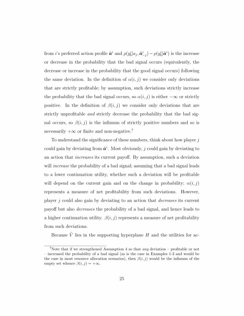
necessarily +∞ or finite and non-negative.7

To understand the significance of these numbers, think about how player j

could gain by deviating from ai. Most obviously, j could gain by deviating to

an action that increases its current payoff. By assumption, such a deviation

will increase the probability of a bad signal; assuming that a bad signal leads

to a lower continuation utility, whether such a deviation will be profitable

will depend on the current gain and on the change in probability; α(i, j)

represents a measure of net profitability from such deviations. However,

player j could also gain by deviating to an action that decreases its current

payoff but also decreases the probability of a bad signal, and hence leads to

a higher continuation utility. β(i, j) represents a measure of net profitability

from such deviations.

Because V lies in the supporting hyperplane H and the utilities for ac-

7Note that if we strengthened Assumption 4 so that any deviation – profitable or not– increased the probability of a bad signal (as is the case in Examples 1-3 and would bethe case in most resource allocation scenarios), then β(i, j) would be the infimum of theempty set whence β(i, j) = +∞.

25

tion profiles not in A lie strictly below H, in order that the strategy profile

σ achieves an efficient payoff it is necessary and sufficient that σ use only

preferred action profiles: U(σ) ∈ V if and only if σ(h) ∈ A for every public

history h (independently of the discount factor δ). For PPE strategies we

can say a lot more. The first Proposition is almost obvious; the second and

third seem far from obvious. (All proofs are in the Appendix.)

Proposition 1. In order that vi be achievable in a PPE equilibrium (for any

discount factor δ) it is necessary and sufficient that uj(aj, ai−j) ≤ uj(a

i) for

every j 6= i and every aj ∈ Aj.

Proposition 2. If σ is an efficient PPE (for any discount factor δ) and i is

active following some history (i.e., σ(h) = ai for some h) then

α(i, j) ≤ β(i, j) (4)

for every j ∈ N, j 6= i.

Proposition 3. If σ is an efficient PPE (for any discount factor δ) and i is

active following some history (i.e., σ(h) = ai for some h) then

vii − ui(ai, a

i−i) ≥

1

λi

∑j 6=i

λj α(i, j)[ρ(yi

b|ai, ai−i)− ρ(yi

b|ai)]

(5)

The import of Propositions 2 and 3 is that if any of these inequalities

fail then certain efficient payoff vectors can never be achieved in PPE, no

26

matter what the discount factor is. In the next Sections, we show how these

inequalities and other conditions yield necessary and sufficient conditions

that certain sets be self-generating and hence yield sufficient conditions for

efficient PPE.

Proposition 2 might seem quite mysterious: α is a measure of the current

gain to deviation and β is a measure of the future gain to deviation; there

seems no obvious reason why PPE should necessitate any particular relation-

ship between α and β. As the proof will show, however, the assumption of

two signals and the efficiency of payoffs in V imply that α is bounded above

and β is bounded below by the same quantity, which is a weighted difference

of continuation values – a quantity that does have an obvious connection to

PPE.

5. Characterizing Efficient Self-Generating Sets

As in the previous Section, we consider a fixed reduced form and maintain

the notation and assumptions of Section 2. In order to find efficient PPE

payoffs we follow APS and look for self-generating sets of efficient payoffs.

Fix a subset W ⊂ co[U(A)] and a target payoff v ∈ co[U(A)]. Recall

from APS that v can be decomposed with respect to W (for a given discount

factor δ < 1) if there exist an action profile a ∈ A and continuation payoffs

γ : Y → W such that

• v is the (weighted) average of current and continuation payoffs when

players follow a

v = (1− δ)U(a) + δ∑y∈Y

ρ(y|a)γ(y)

27

• continuation payoffs provide no incentive to deviate: for each j and

each aj ∈ Aj

vj ≥ (1− δ)U(aj,a−j) + δ∑y∈Y

ρ(y|aj,a−j)γ(y)

Write B(W, δ) for the set of target payoffs v ∈ co[U(A)] that can be de-

composed with respect to W (for the discount factor δ. Recall that W is

self-generating if W ⊂ B(W, δ); i.e., every target vector in W can be decom-

posed with respect to W .

Because V lies in the hyperplane H, if v ∈ V and it is possible to de-

compose v ∈ V with respect to any set and for any discount factor, then

the associated action profile a must lie in A and the continuation payoffs

must lie in V . Because we are interested in efficient payoffs we can therefore

restrict our search for self-generating sets to subsets W ⊂ V . In order to

understand which sets W ⊂ V can be self-generating, we need to understand

how players might profitably gain from deviating from the current recom-

mended action profile. Because we are interested in subsets W ⊂ V , the

current recommended action profile will always be ai for some i, so we need

to ask how a player j might profitably gain from deviating from ai. For

player j 6= i, a profitable deviation might occur in one of two ways: j might

gain by choosing an action aj 6= aij that increases j’s current payoff or by

choosing an action aj 6= aij that alters the signal distribution in such a way

as to increase j’s future payoff. Because ai yields i its best current payoff,

a profitable deviation by i might occur only by choosing an action that that

alters the signal distribution in such a way as to increase i’s future payoff. In

28

all cases, the issue will be the net of the current gain/loss against the future

loss/gain.

We focus attention on sets of the form

Vµ = v ∈ V : vi ≥ µi for each i

where µ ∈ Rn; we assume without further comment that Vµ 6= ∅. For lack of

a better term, we say that Vµ is regular if for each i ∈ N there is a vector

vi ∈ Vµ such that vij = µj for each j 6= i. Whether or not Vµ is regular

depends both on the shape of V and on the magnitude of µ: see Figures 2,

3, 4 for instance. A few simple facts are useful to note:

• If vij = 0 for all i, j ∈ N with i 6= j (as is the case in many resource

sharing scenarios such as Examples 2, 3) then Vµ is regular for every

µ ≥ 0.

• If Vµ 6= ∅ and Vµ is a subset of the interior of V (relative to the hyper-

plane H) then Vµ is regular.

• If v lies in the interior of V (relative to the hyperplane H) and µ =

v − ε · 1 for ε > 0 sufficiently small, then v ∈ Vµ and Vµ is regular.

• If Vµ is not a singleton then it must contain a point of the interior of

V (relative to the hyperplane H).

If Vµ is a singleton, it can only be a self-generating set (and hence achievable

in a PPE) if Vµ = vi for i; because we have already characterized this pos-

sibility in Proposition 1, we focus on the non-degenerate case in which Vµ is

not a singleton and hence contains a point of the interior of V . Note that a

29

Figure 2: µ = (0, 1/4, 0); Vµ is regular

Figure 3: µ = (1/2, 1/2, 1/2); Vµ is regular

point in the interior of V can only be achieved by a repeated game strategy

in which all players are active following some history.

The following result provides necessary and sufficient conditions on µ,

the payoff structure, the information structure and the discount factor that

a regular Vµ be a self-generating set.

Theorem 1. Fix µ; assume that Vµ is regular and not an extreme point of

V . In order that Vµ be a self-generating set, it is necessary and sufficient

that the following conditions be satisfied:

30

Figure 4: µ = (1/4, 0, 0); Vµ is not regular

Condition 1 for all i, j ∈ N with i 6= j:

α(i, j) ≤ β(i, j) (6)

Condition 2 for all i ∈ N and all ai ∈ Ai:

vii − ui(ai, a

i−i) ≥

1

λi

∑j 6=i

λj α(i, j)[ρ(yi

b|ai, ai−i)− ρ(yi

b|ai)]

(7)

Condition 3 for all i ∈ N :

µi ≥ maxj 6=i

(vj

i + α(j, i)[1− ρ(yjb |aj)]

)(8)

Condition 4 the discount factor δ satisfies:

δ ≥ δµ ,

1 +1−∑

iλiµi

∑i

[λivi

i +∑j 6=i

λj α(i, j) ρ(yib|ai)

]− 1

−1

(9)

31

One way to contrast our approach with that of FLM (and FLT) is to think

about the constraints that need to be satisfied to decompose a given target

payoff v with respect to a given set Vµ. By definition we must find a current

action profile a and continuation payoffs γ. The achievability condition (that

v is the weighted combination of the utility of the current action profile

and the expected continuation values) yields a family of linear equalities.

The incentive compatibility conditions (that players must be deterred from

deviating from a) yields a family of linear inequalities. In the context of

FLM, satisfying all these linear inequalities simultaneously requires a large

and rich collection of signals so that many different continuation payoffs can

be assigned to different deviations. Because we have only two signals, we are

only able to choose two continuation payoffs but still must satisfy the same

family of inequalities – so our task is much more difficult. It is this difficulty

that leads to the Conditions in Theorem 1.

Note that δµ is decreasing in µ. Since Condition 3 puts an absolute lower

bound on µ and Condition 4 puts an absolute lower bound on δµ this means

that (subject to the regularity constraint) there is a µ∗ such that Vµ∗ is

the largest self-generating set (of this form) and δµ∗ is the smallest discount

factor (for which any set of this form can be self-generating). This may seem

puzzling – increasing the discount factor beyond a point makes no difference

– but remember that we are providing a characterization of self-generating

sets and not of PPE payoffs. However, as we shall see in Theorem 4, for the

two-player case, we do obtain a complete characterization of (efficient) PPE

payoffs and we demonstrate the same phenomenon.

32

6. Perfect Public Equilibrium

Because every payoff in a self-generating set can be achieved in a PPE,

Theorem 1 immediately provides sufficient conditions achieving (some) given

target payoffs in perfect public equilibrium. In fact, we can provide an explicit

algorithm for computing PPE strategies. A consequence of this algorithm is

that (at least when action spaces are finite), the constructed PPE enjoys an

interesting and potentially useful robustness property.

6.1. A Constructing Efficient Perfect Public Equilibria

Given the various parameters of the environment (game payoffs, infor-

mation structure, discount factor) and of the problem (lower bound, target

vector), the algorithm takes as input in period t the current continuation

vector v(t) and computes, for each player j, an indicator dj(v(t)) defined as

follows:

dj(v(t)) =λj[vj(t)− µj]

λj[vjj − vj(t)] +

∑k 6=j λk α(j, k)ρ(yj

b |aj)

(Note that each player can compute every dj from the current continuation

vector v(t) and the various parameters.) Having computed dj(v(t)) for each

j, the algorithm finds the player i∗ whose indicator is greatest. (In case of

ties, we arbitrarily choose the player with the largest index.) The current

action profile is i∗’s preferred action profile ai∗ . The algorithm then uses the

labeling Y = yi∗g , y

i∗b to compute continuation values for each signal in Y .

Theorem 2. If the conditions in Theorem 1 are satisfied, then every payoff

v ∈ Vµ can be achieved in a PPE. For v ∈ Vµ, a PPE strategy profile that

achieves v can be computed by the algorithm in Table 2

33

Table 2: The algorithm used by each player.

Input: The current continuation payoff v(t) ∈ Vµ

For each j

Calculate the indicator dj(v(t))

Find the player i with largest indicator (if a tie, choose largest i)

i = maxj arg maxj∈N dj(v(t))Player i is active; chooses action ai

i

Players j 6= i are inactive; choose action aij

Update v(t+ 1) as follows:

if yt = yig then

vi(t+ 1) = vii + (1/δ)(vi(t)− vi

i)− (1/δ − 1)(1/λi)∑

j 6=i λjα(i, j)ρ(yib|ai)

vj(t+ 1) = vij + (1/δ)(vj(t)− vi

j) + (1/δ − 1)α(i, j)ρ(yib|ai)

for all j 6= i

if yt = yib then

vi(t+ 1) = vii + (1/δ)(vi(t)− vi

i) + (1/δ − 1)(1/λi)∑

j 6=i λjα(i, j)ρ(yig|ai)

vj(t+ 1) = vij + (1/δ)(vj(t)− vi

j)− (1/δ − 1)α(i, j)ρ(yig|ai)

for all j 6= i

34

6.2. Robustness

A consequence of our constructive algorithm is that, for generic values

of the parameters of the environment and of the problem and for as many

periods as we specify, the strategies we identify are locally constant in these

parameters. To make this precise, we assume for this subsection that action

spaces Ai are finite. The parameters of the model are the utility mapping

U : A → Rn and the probabilities ρ(·|·) : Y × A → [0, 1]. Because the

probabilities must sum to 1 and we require full support, the parameter space

of the model is

Ω = (Rn × [0, 1])A

The parameters of the problem are the discount factor δ, the constraint vector

µ and the target profile v∗; because the target profile lies in a hyperplane,

the parameter space for the particular problem is

Θ = (0, 1)× Rn × Rn−1

Let Ξ ⊂ Ω × Θ be the subset of parameters that satisfy the Conditions of

Theorem 1. For ξ ∈ Ξ, the algorithm generates an strategy profile

σξ : H → A

For T ≥ 0 we write σTξ for the restriction of σξ to the set HT of histories of

length at most T .

Theorem 3. For each T ≥ 0 there is a subset ΞT ⊂ Ξ that is closed and has

measure 0 with the property that the mapping ξ → σTξ : Ξ → HT is locally

35

constant on the complement of ΞT .

In words: if ξ, ξ′ are close together and neither lies in the proscribed small

set of parameters ΞT , then the strategies σξ, σξ′ coincide for at least the first

T periods.

6.3. Comparison with FLT

As we have commented in the Introduction, our approach provides a great

deal of information about the efficient payoffs that can be achieved in PPE

but because the sets Vµ are required to have a special form, it does not find

all of them. Here we provide a simple example. We consider a 3 × 3 game.

Each player chooses from the actions l,m, h: Player 1 chooses rows, Player

2 chooses columns, Player 3 chooses matrices; see Table 3. (Payoffs indicated

by ∗ are irrelevant so long as Assumptions 1,2 are satisfied; we could take

∗ = 0 everywhere.) There are two signals yg, yb and the signal structure is

ρ(yg|a) =

2/3 if a = (h, `, `) or any permutation

1/2 if a = (h,m, `) or any permutation

1/3 otherwise

Note that a1 = (h, `, `), a2 = (`, h, `), a3 = (`, `, h) and that v1 = (1, .5, 0),

v2 = (0, 1, .5), v3 = (.5, 0, 1). Condition 3 implies that no regular Vµ can be

a self-generating set (because we would have to have µi > .5 for each i), so

our approach does not find any PPE. However, applying the machinery of

FLT shows that there is a discount factor δ < 1 for which the payoff vector

(.5, .5, .5) – indeed, any efficient payoff vector close to (.5, .5, .5) – can be

36

Table 3: Payoff Matrices for the 3× 3 Game; Player 3 Chooses `, m, h (respectively)

` m h` (∗, ∗, ∗) (∗, ∗, ∗) (0, 1, 0.5)m (∗, ∗, ∗) (∗, ∗, ∗) (0.1, ∗, ∗)h (1, 0.5, 0) (∗, 0.55, ∗) (0.2, 0.6, ∗)

` m h` (∗, ∗, ∗) (∗, ∗, ∗) (∗, ∗, 0.55)m (∗, ∗, ∗) (∗, ∗, ∗) (∗, ∗, ∗)h (∗, ∗, 0.1) (∗, ∗, ∗) (∗, ∗, ∗)

` m h` (0.5, 0, 1) (∗, 0.1, ∗) (∗, 0.2, 0.6)m (0.55, ∗, ∗) (∗, ∗, ∗) (∗, ∗, ∗)h (0.6, ∗, 0.2) (∗, ∗, ∗) (∗, ∗, ∗)

achieved in PPE.8 As noted in the Introduction, however, FLT provides no

information as to what δ must be nor does it construct PPE strategies.

7. Two Players

Theorem 1 provides a complete characterization of self-generating sets

that have a special form. If there are only two players then maximal self-

generating sets – the set of all PPE – have this form and so it is possible to

provide a complete characterization of PPE. We focus on what seems to be

the most striking finding: either there are no efficient PPE outcomes at all

(for any discount factor δ < 1) or there is a discount factor δ∗ < 1 with the

8Calculations available from the authors by request.

37

property that any target payoff in V that can be achieved as a PPE for some

δ can already be achieved for every δ ≥ δ∗.

Theorem 4. Assume N = 2 (two players). Either

(i) no target profile in V can be supported in a PPE for any δ < 1 or

(ii) there exist µ1, µ2 and a discount factor δ∗ < 1 such that if δ is any

discount factor with δ∗ ≤ δ < 1 then the set of payoff vectors that can

be supported in a PPE when the discount factor is δ is precisely

E = v ∈ V : vi ≥ µi for i = 1, 2

The proof yields explicit (messy) expressions for µ1, µ2 and δ∗.

38

8. Examples, Redux

In Section 3 we presented three examples to illustrate the model. We now

return to these models to illustrate our analysis and conclusions.

Example 1 Because there are only two players, Theorem 4 applies. In this

case it is easy to give explicit expressions for µ1, µ2 and for the threshold

discount factor δ∗.9 In fact µ1 = µ12 = q/(q − r)b and

δ∗ =1

1 +(

B−2 qq−r

b

B+2 1−qq−r

b

)

so that for every δ ≥ δ∗ the set of efficient payoffs that can be achieved in

PPE is exactly

E(δ) = (v1, v2) : v1 + v2 = B; vi ≥ q/(q − r)b

We stress that the set of efficient equilibrium outcomes does not increase as

δ → 1; as we noted in the Introduction, patience is rewarded but only up to

a point. See Figure 5.

Example 2 As we have noted, the choice of a reporting rule has implications

for the equilibria of the repeated game. In this case it is natural to consider

two reporting rules (Y 1, ψ1), (Y 2, ψ2) where

• Y 1 = yb, yg; ψ1(zk) = yb if k = 0, ψ1(zk) = yg if k 6= 0

• Y 2 = Z; ψ2(zk) = zk for all k = 0, . . . , n

9Calculations are available from the authors on request.

39

COL

ROW

Pareto optimal PPE payoff profiles

(b, b)

(c, c)

(0, B)

(B, 0)

Figure 5: Efficient PPE Payoffs for the Modified Prisoners’ Dilemma.

In the first rule (which is the one discussed in Section 3), the designer an-

nounces whether or not there has been a winner; in the second case the

designer also announces the identity of the winner.

As we have noted earlier, in the reduced forms of the stage game, the ex

ante expected utilities are given by

Ui(a) = ai

η − κ∑j 6=i

aj

+

R− cai

and, with the first reporting rule, the signal distribution is

ρ(y∗|a)

1−∑

i ai

(η − κ

∑j 6=i aj

)+if ∗ = b∑

i ai

(η − κ

∑j 6=i aj

)+if ∗ = g

40

With the second reporting rule, the signal distribution is

ρ(yk|a) =

1−∑

i ai

(η − κ

∑j 6=i aj

)+if k = 0

ak

(η − κ

∑j 6=k aj

)+if k 6= 0

To be specific, suppose there are 2 players. With the first reporting rule,

there are two signals; with the second reporting rule there are three signals.

The second reporting rule provides additional information to players and

this additional information can be used to support more PPE. Suppose for

instance that a strategy profile σ calls for a1 to be played after a particular

history. If all the players follow σ then only player 1 exerts non-zero effort so

only two outcomes can occur: either player 1 wins or no one wins. If player 2

deviates by exerting non-zero effort, a third outcome can occur: 2 wins. With

either monitoring structure, it is possible for player 1 to detect (statistically)

when player 2 has deviated, but with the second monitoring structure it

will sometimes be the case that player 1 can be certain that player 2 has

deviated. This additional information makes it possible to provide additional

punishments for deviation and hence to support a larger set of efficient PPE.

As Figure 6 shows, the difference matters: the second reporting rule always

supports a larger set of efficient PPE; indeed, for some values of κ (which

measures the strength of the interference) only the second reporting rule

supports any efficient PPE at all.

More generally, consider a context with n ≥ 3 players. If the identity of

the winner is not announced, all deviations must be “punished” in the same

way, but if the identity of the winner is announced, “punishments” can be

tailored to the deviator, and hence can be more severe. If punishments can

41

0.45 0.5 0.55 0.6 0.65 0.70

0.1

0.2

0.3

0.4

0.5

0.6

0.7

0.8

0.9

1

κ

Larg

est A

chie

vabl

e F

ract

ions

3 signals2 signals

Figure 6: Largest Achievable Fraction 1− µi/vii as a Function of κ.

42

be more severe it may be possible to sustain a wider range of PPE. Which

reporting rule – hence which monitoring structure – should be chosen by the

designer will depend on the tradeoff the designer makes between preserving

privacy and sustaining a wider range of PPE.

Example 3 As we have suggested, the designer must choose from some

(possible) measurement technologies. This choice involves a tension: more

accurate measurement technologies will typically be more costly to employ.

Hence the designer must trade-off the accuracy of the measurement tech-

nology against the cost of employing it. The designer must also choose a

reporting rule, in this case a threshold d0. This choice also involves a ten-

sion, but of a different kind. Given the distribution of shocks and a choice

of measurement technology, the choice of threshold affects the distribution

of signals. How the designer chooses the distribution of signals depends on

what the designer wishes to accomplish. For instance, given a fixed discount

factor, the designer may wish to choose the threshold to maximize the range

of long-run resource allocations that can be supported as PPE for the given

discount factor. Alternatively, the designer may wish to minimize the dis-

count factor for which some long-run resource allocation can be supported

as a PPE.

To give some idea of the effect of these tradeoffs, we present numerical

results for a special case of the Resource Sharing Game with 3 players, ca-

pacity χ = 1 and ε = 0.3. Because the game is symmetric it seems natural

to consider symmetric sets of payoffs; so we consider sets of the form

V (η) = v ∈ V : vi ≥ ηv for each i

43

0 5 10 15 20 25 30 350.88

0.9

0.92

0.94

0.96

0.98

1

The threshold

Larg

est A

chie

vabl

e F

ract

ions

p=1.2p=1.5p=2.0

Figure 7: Largest Achievable Fraction 1− η as a Function of Threshold d0.

where v is the utility of each player’s most preferred action and η ∈ [0, 1].

Note that 1 − η represents the fraction of the entire efficient set V that is

occupied by V (η). A natural desideratum for the designer is to choose the

threshold d0 so that the fraction 1− η is as large as possible; this maximizes

opportunities for sharing. (As we have shown in Theorem 1, making η smaller

also makes the required discount factor smaller, so the designer can simulta-

neously create more sharing opportunities for less patient players.) Figures

7 and 8 display (from simulations) the relationship between the threshold d0

and the smallest η and smallest δ for different values of the exponent p.

44

0 5 10 15 20 25 30 350.66

0.68

0.7

0.72

0.74

0.76

0.78

0.8

The threshold

Low

er b

ound

dis

coun

t fac

tor

p=1.2p=1.5p=2.0

Figure 8: Smallest Achievable Discount Factor δ as a Function of Threshold d0

45

9. Conclusion

This paper diverges from much of the familiar literature on repeated

games with imperfect public monitoring in two directions. In analyzing the

reduced form, we make different assumptions on the signal structure and ob-

tain stronger conclusions about efficient PPE (bounds on the discount factor,

explicitly constructive strategies). However, we also construct an elaborated

form in which the information structure can be viewed as arising from the

behavior of a strategic designer. Clearly there is much more to be done.

Perhaps most obviously, it is clearly important to understand the extent to

which the assumptions on the signal structure of the reduced form and on the

geometry of the candidate self-generating sets Vµ can be relaxed. However,

we think the elaborated form is of even more potential interest, especially

for applications. As we have discussed in the Examples, the designer must

decide what to observe and what to communicate to the players, and these

choices will typically involve a trade-off between the cost of more accurate

observation and communication on the one hand and the benefits of bet-

ter information on the other hand. It seems natural to suppose that the

costs and benefits – and hence the trade-offs – may be very different across

environments. This seems a subject worthy of much study.

References

Abreu, D., Pearce, D., Stacchetti, E., 1990. Toward a theory of discounted

repeated games with imperfect monitoring. Econometrica 58 (5), 1041–

1063.

46

Athey, S., Bagwell, K., 2001. Optimal collusion with private information.

RAND Journal of Economics 32 (3), 428–465.

Bharath-Kumar, K., Jaffe, J. M., 1981. A new approach to performance-

oriented flow control. IEEE Transactions on Communications 29 (4), 427–

435.

Blume, L. E., Zame, W. R., 1994. The algebraic geometry of perfect and

sequential equilibrium. Econometrica 62 (4), 783–794.

Bochnak, J., Coste, M., Roy, M.-F., 1998. Real algebraic geometry. Springer.

Fudenberg, D., Levine, D. K., Maskin, E., 1994. The folk theorem with

imperfect public information. Econometrica 62 (5), 997–1039.

Fudenberg, D., Levine, D. K., Takahashi, S., 2007. Perfect public equilibrium

when players are patient. Games and Economic Behavior 61 (1), 27 – 49.

Green, E. J., Porter, R. H., 1984. Noncooperative collusion under imperfect

price information. Econometrica 52 (1), 87–100.

Mailath, G., Obara, I., Sekiguchi, T., 2002. The maximum efficient equi-

librium payoff in the repeated prisoners’ dilemma. Games and Economic

Behavior 40 (1), 99–122.

Mailath, G., Samuelson, L., 2006. Repeated Games and Reputations: Long-

run Relationships. Oxford University Press, Oxford, U.K.

47

Appendix

The proof of Proposition 1 is immediate and omitted.

Proof of Proposition 2 Fix an active player i and an inactive player j.

Set

A(i, j) =aj ∈ Aj : uj(aj, a

i−j) > uj(a

i)

B(i, j) =aj ∈ Aj : uj(aj, a

i−j) < uj(a

i), ρ(yib|aj, a

i−j) < ρ(yi

b|ai)

If either of A(i, j) or B(i, j) is empty then α(i, j) ≤ β(i, j) by default, so

assume in what follows that neither of A(i, j), B(i, j) is empty.

Fix a discount factor δ ∈ (0, 1) and let σ be PPE that achieves an ef-

ficient payoff. Assume that i is active following some history: σ(h) = ai

for some h. Because σ achieves an efficient payoff, we can decompose the

payoff v following h as the weighted sum of the current payoff from ai and

the continuation payoff assuming that players follow σ; because σ is a PPE,

the incentive compatibility condition for all players j must obtain. Hence for

all aj ∈ Aj we have

vj = (1− δ)uj(ai) + δ

∑y∈Y

ρ(y|ai)γj(y)

≥ (1− δ)uj(aj, ai−j) + δ

∑y∈Y

ρ(y|aj, ai−j)γj(y), (10)

48

Substituting probabilities for the good and bad signals yields

vj = (1− δ)uj(ai) + δ

[ρ(yi

g|ai)γj(yig) + ρ(yi

b|ai)γj(yib)]

≥ (1− δ)uj(aj, ai−j) + δ

[ρ(yi

g|aj, ai−j)γj(y

ig) + ρ(yi

b|aj, ai−j)γj(y

ib)]

Rearranging yields

[ρ(yi

b|aj, ai−j)− ρ(yi

b|ai)][γj(y

ig)− γj(y

ib)][

δ

1− δ

]≥[uj(aj, a

i−j)− uj(a

i)]

Now suppose j 6= i is an inactive player. If aj ∈ A(i, j) then ρ(yib|aj, a

i−j)−

ρ(yib|ai) > 0 (by Assumption 4) so

[γj(y

ig)− γj(y

ib)][

δ

1− δ

]≥

uj(aj, ai−j)− uj(a

i)

ρ(yib|aj, ai

−j)− ρ(yib|ai)

(11)

If aj ∈ B(i, j) then ρ(yib|aj, a

i−j)− ρ(yi

b|ai) < 0 (by definition) so

[γj(y

ig)− γj(y

ib)][

δ

1− δ

]≤

uj(aj, ai−j)− uj(a

i)

ρ(yib|aj, ai

−j)− ρ(yib|ai)

(12)

Taking the sup over aj ∈ A(i, j) in (11) and the inf over aj ∈ B(i, j) in (12)

yields α(i, j) ≤ β(i, j) as desired.

Proof of Proposition 3 As above, we assume i is active following the

history h and that v is the payoff following h. Fix ai ∈ Ai. By definition,

ui(ai) > ui(ai, a

i−i). With respect to probabilities, there are two possibilities.

49

If ρ(yib|ai, a

i−i) ≤ ρ(yi

b|ai) then we immediately have

vii − ui(ai, a

i−i) ≥

1

λi

∑j 6=i

λjα(i, j)[ρ(yib|ai, a

i−i)− ρ(yi

b|ai)]

because the left-hand side is positive and the right-hand side is non-negative.

If ρ(yib|ai, a

i−i) > ρ(yi

b|ai) we proceed as follows.

We begin with (10) but now we apply it to the active user i, so that for

all ai ∈ Ai we have

vi = (1− δ)ui(ai) + δ

[ρ(yi

g|ai)γi(yig) + ρ(yi

b|ai)γi(yib)]

≥ (1− δ)ui(ai, ai−i) + δ

[(ρ(yi

g|ai, ai−i)γi(y

ig) + ρ(yi

b|ai, ai−i)γi(y

ib)]

Rearranging yields

γi(yig)− γi(y

ib) ≥

[1− δ

δ

] [ui(ai, a

i−i)− ui(a

i)

ρ(yib|ai, ai

−i)− ρ(yib|ai)

]

Because continuation payoffs are in V , which lies in the hyperplane H, the

continuation payoffs for the active user can be expressed in terms of the

continuation payoffs for the inactive users as

γi(y) =1

λi

1−∑j 6=i

λjγj(y)

Hence

γi(yig)− γi(y

ib) = − 1

λi

∑j 6=i

λj[γj(yig)− γj(y

ib)]

Applying the incentive compatibility constraints for the inactive users implies

50

that for each aj ∈ A(i, j) we have

γj(yig)− γj(y

ib) ≥

[1− δ

δ

] [uj(aj, a

i−j)− uj(a

i)

ρ(yib|aj, ai

−j)− ρ(yib|ai)

]

In particular

γj(yig)− γj(y

ib) ≥

[1− δ

δ

]α(i, j)

and hence

γi(yig)− γi(y

ib) ≤ − 1

λi

[1− δ

δ

] ∑j 6=i

λjα(i, j)

≤ 0

Putting these all together, canceling the factor [1 − δ]/δ and remembering

that we are in the case ρ(yib|ai, a

i−i) > ρ(yi

b|ai) yields

vii − ui(ai, a

i−i) ≥

1

λi

∑j 6=i

λjα(i, j)[ρ(yib|ai, a

i−i)− ρ(yi

b|ai)]

which is the desired result.

Proof of Theorem 1 Assume that Vµ is regular and not an extreme point,

and is a self-generating set; we verify Conditions 1-4 in turn. Because Vµ is

self-generating and not an extreme point, it cannot be a singleton and hence

must contain an interior point of V . In order for such a point to be achieved

in a PPE, every player must be active following some history, so Propositions

2 and 3 yield Conditions 1 and 2.

By assumption, for each i ∈ N there is a payoff profile vi ∈ Vµ with the

property that vij = µj for each j 6= i. Necessarily, vi is the unique such point

51

and vi = arg maxvi : v ∈ Vµ. Because V lies in the hyperplane H we have

vij =

µj if j 6= i

1λi

(1−∑

k 6=i λkµk

)if j = i

Because Vµ is self-generating, we can decompose vi:

vi = (1− δ)u(ak) + δ∑y

ρ(y|ak)γ(y) (13)

for some ak. If k 6= i then (because Vµ 6= vk) we must have µk < vkk which

implies that γk(y) < µk for some y; since continuation payoffs must lie in

Vµ this is a contradiction. Hence in the decomposition (13) we must have

ak = ai.

It is convenient to first establish the following inequality on µj on the way

to establishing the bounds in Condition 3.

µj > maxi6=j

vij for all j ∈ N

To see this, suppose to the contrary that there exists a i, j such that µj ≤ vij.

Consider i’s preferred payoff profile vi in Vµ. Because decomposing vi requires

that we use ai, it follows that

µj = (1− δ) · vij + δ ·

∑y

ρ(y|ai)γj(y)

If µj < vij then

∑y∈Y ρ(y|ai)γi(y) < µj and so γj(y) < µj for some y.

This contradicts that fact that γ(y) ∈ Vµ. If µj = vij, we must have

52

∑y ρ(y|ai)γj(y) = µj. Since γj(y) ≥ µj for all y, we must have γj(y

ig) =

γj(yib) = µj. By assumption, player j has a currently profitable deviation

aj so that uj(aj, ai−j) > uj(a

i), which implies that the continuation payoff

γj(yig) = γj(y

ib) = µj cannot satisfy the incentive compatibility constraints.

Hence, we must have µj > vij as asserted.

With all this in hand we derive Condition 3. To do this, we suppose i

is active and examine the decomposition of the inactive player j’s payoff in

greater detail. Because µj > vij and vj ≥ µj for every v ∈ Vµ we certainly

have vj > vij. We can write j’s incentive compatibility condition as

vj = (1− δ) · vij + δ ·

∑y∈Y

ρ(y|ai) · γj(y) (14)

≥ (1− δ) · uj(aj, ai−j) + δ ·

∑y∈Y

ρ(y|aj, ai−j) · γj(y).

From the equality constraint in (14), we can solve for the discount factor δ

as

δ =vj − vi

j∑y∈Y γj(y)ρ(y|ai)− vi

j

(Note that the denominator can never be zero and the above equation is well

defined, because vj > vij implies that

∑y∈Y γj(y)ρ(y|ai) > vi

j.) We can then

eliminate the discount factor δ in the inequality of (14). Since vj > vij, we

can obtain equivalent inequalities, depending on whether aj is a profitable

or unprofitable current deviation):

53

• If uj(aj, ai−j) > vi

j then

vj ≤∑y∈Y

γj(y)

[(1−

vj − vij

uj(aj, ai−j)− vi

j

)ρ(y|ai)

+vj − vi

j

uj(aj, ai−j)− vi

j

ρ(y|aj, ai−j)

](15)

• If uj(aj, ai−j) < vi

j then

vj ≥∑y∈Y

γj(y)

[(1−

vj − vij

uj(aj, ai−j)− vi

j

)ρ(y|ai)

+vj − vi

j

uj(aj, ai−j)− vi

j

ρ(y|aj, ai−j)

](16)

For notational convenience, write the coefficient of γj(yig) in the above

inequalities as

cij(aj, ai−j) ,

(1−

vj − vij

uj(aj, ai−j)− vi

j

)ρ(yi

g|ai)

+

(vj − vi

j

uj(aj, ai−j)− vi

j

)ρ(yi

g|aj, ai−j)

= ρ(yig|ai) + (vj − vi

j)

(ρ(yi

g|aj, ai−j)− ρ(yi

g|ai)

uj(aj, ai−j)− vi

j

)

= ρ(yig|ai)− (vj − vi

j)

(ρ(yi

b|aj, ai−j)− ρ(yi

b|ai)

uj(aj, ai−j)− vi

j

)

According to (15), if uj(aj, ai−j) > vi

j then

cij(aj, ai−j) · γj(y

ig) +

[1− cij(aj, a

i−j)]γj(y

ib) ≤ vj (17)

54

Since γj(yig) > γj(y

ib), this is true if and only if

κ+ij · γj(y

ig) + (1− κ+

ij) · γj(yib) ≤ vj, (18)

where κ+ij , supcij(aj, a

i−j) : aj ∈ Aj : uj(aj, a

i−j) > vi

j. (Fulfilling the

inequalities (17) for all aj such that uj(aj, ai−j) > uj(a

i) is equivalent to ful-

filling the single inequality (18). If (18) is satisfied, then the inequalities (17)

are satisfied for all aj such that uj(aj, ai−j) > uj(a

i) because γj(yig) > γj(y

ib)

and κ+ij ≥ cij(aj, a

i−j) for all aj such that uj(aj, a

i−j) > uj(a

i). Conversely, if

the inequalities (17) are satisfied for all aj such that uj(aj, ai−j) > uj(a

i) and

(18) were violated, so that κ+ij ·γj(y

ig)+(1−κ+

ij) ·γj(yib) > vj, then we can find

a κ′ij < κ+ij such that κ′ij ·γj(y

ig)+(1−κ′ij)·γj(y

ib) > vj. Based on the definition

of the supremum, there exists at least a a′j such that uj(a′j, a

i−j) > uj(a

i) and

cij(a′j, a

i−j) > c′ij, which means that cij(a

′j, a

i−j) · γj(y

ig) + (1 − cij(a

′j, a

i−j)) ·

γj(yib) > vj. This contradicts the fact that the inequalities (18) are fulfilled

for all aj such that uj(aj, ai−j) > uj(a

i).)

Similarly, according to (16), for all aj such that uj(aj, ai−j) < vi

j, we must

have

cij(aj, ai−j)γj(y

ig) + [1− cij(aj, a

i−j)]γj(y

ib) ≥ vj.

Since γj(yig) > γj(y

ib), the above requirement is fulfilled if and only if

κ−ij · γj(yig) + (1− κ−ij) · γj(y

ib) ≥ vj,

where κ−ij , infcij(aj, a

i−j) : aj ∈ Aj, uj(aj, a

i−j) < vi

j

. Hence, the decom-

55

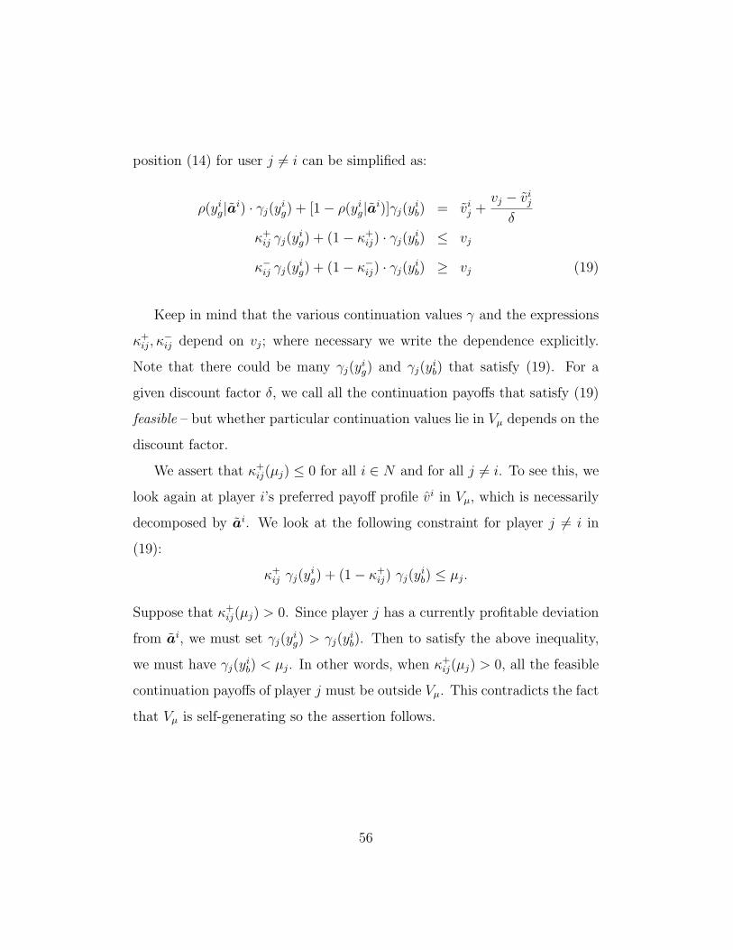
position (14) for user j 6= i can be simplified as:

ρ(yig|ai) · γj(y

ig) + [1− ρ(yi

g|ai)]γj(yib) = vi

j +vj − vi

j

δ

κ+ij γj(y

ig) + (1− κ+

ij) · γj(yib) ≤ vj

κ−ij γj(yig) + (1− κ−ij) · γj(y

ib) ≥ vj (19)

Keep in mind that the various continuation values γ and the expressions

κ+ij, κ

−ij depend on vj; where necessary we write the dependence explicitly.

Note that there could be many γj(yig) and γj(y

ib) that satisfy (19). For a

given discount factor δ, we call all the continuation payoffs that satisfy (19)

feasible – but whether particular continuation values lie in Vµ depends on the

discount factor.

We assert that κ+ij(µj) ≤ 0 for all i ∈ N and for all j 6= i. To see this, we

look again at player i’s preferred payoff profile vi in Vµ, which is necessarily

decomposed by ai. We look at the following constraint for player j 6= i in

(19):

κ+ij γj(y

ig) + (1− κ+

ij) γj(yib) ≤ µj.

Suppose that κ+ij(µj) > 0. Since player j has a currently profitable deviation

from ai, we must set γj(yig) > γj(y

ib). Then to satisfy the above inequality,

we must have γj(yib) < µj. In other words, when κ+

ij(µj) > 0, all the feasible

continuation payoffs of player j must be outside Vµ. This contradicts the fact

that Vµ is self-generating so the assertion follows.

56

The definition of κ+ij(µj) and the fact that κ+

ij(µj) ≤ 0 entail that

κ+ij(µj) = ρ(yi

g|ai)− (µj − vij) inf

aj∈A(i,j)

[ρ(yi

b|aj, ai−j)− ρ(yi

b|ai)

uj(aj, ai−j)− vi

j

]

= ρ(yig|ai)− (µj − vi

j)

1

supaj∈A(i,j)

(uj(aj ,ai

−j)−vij

ρ(yib|aj ,ai

−j)−ρ(yib|ai)

)

= ρ(yig|ai)− (µj − vi

j)

[1

α(i, j)

]≤ 0

This provides a lower bound on µj:

µj ≥ vij + α(i, j)ρ(yi

g|ai) = vij + α(i, j)[1− ρ(yi

b|ai)]

This bound must hold for every i ∈ N and every j 6= i. Hence, we have

µj ≥ maxi6=j

(vi

j + α(i, j)[1− ρ(yib|ai)]

)

which is Condition 3.

Now we derive Condition 4 (the necessary condition on the discount fac-

tor). The minimum discount factor δµ required for Vµ to be a self-generating

set solves the optimization problem

δµ = maxv∈Vµ

δ subject to v ∈ B(Vµ; δ)

where B(Vµ; δ) is the set of payoff profiles that can be decomposed on Vµ

under discount factor δ. Since B(Vµ; δ) = ∪i∈NB(Vµ; δ, ai), the above opti-

57

Decomposition equality

IC constraint(currently profitable deviation)

IC constraint(currently unprofitable deviation)

Feasible continuation payoffs

Figure 9: Illustrations of the feasible continuation payoffs when κ+ij ≤ 0. γj =

1λj

(1−

∑k 6=j λkµk

).

mization problem can be reformulated as

δµ = maxv∈Vµ

mini∈N

δ subject to v ∈ B(Vµ; δ, ai). (20)

To solve the optimization problem (20), we explicitly express the constraint

v ∈ B(Vµ; δ, ai) using the results derived above.

Some intuition may be useful. Suppose that i is active and j is an inactive

player. Recall that player j’s feasible γj(yig) and γj(y

ib) must satisfy (19).

There are many γj(yig) and γj(y

ib) that satisfy (19). In Fig. 9, we show the

feasible continuation payoffs that satisfy (19) when κ+ij(vj) ≤ 0. We can

see that all the continuation payoffs on the heavy line segment are feasible.

The line segment is on the line that represents the decomposition equality

ρ(yig|ai) · γj(y

ig) + (1 − ρ(yi

g|ai)) · γj(yib) = vi

j +vj−vi

j

δ, and is bounded by

the IC constraint on currently profitable deviations κ+ij · γj(y

ig) + (1 − κ+

ij) ·

58

γj(yib) ≤ vj and the IC constraint on currently unprofitable deviations κ−ij ·

γj(yig) + (1 − κ−ij) · γj(y

ib) ≥ vj. Among all the feasible continuation payoffs,

denoted γ′(y), we choose the one, denoted γ∗(y), such that for all j 6= i,

γ∗j (yig) and γ∗j (y

ib) make the IC constraint on currently profitable deviations

in (19) binding. This is because under the same discount factor δ, if there

is any feasible continuation payoff γ′(y) in the self-generating set, the one

that makes the IC constraint on currently profitable deviations binding is

also in the self-generating set. The reason is that, as can be seen from Fig. 9,

the continuation payoff γ∗j (y) that makes the IC constraint binding has the

smallest γ∗j (yig) = min γ′j(y

ig) and the largest γ∗j (y

ib) = max γ′j(y

ib). Formally

we establish the following Lemma.

Lemma 1. Fix a payoff profile v and a discount factor δ. Suppose that v is

decomposed by ai. If there are any feasible continuation payoffs γ′(yig) ∈ Vµ

and γ′(yib) ∈ Vµ that satisfy (19) for all j 6= i, there there exist feasible

continuation payoffs γ∗(yig) ∈ Vµ and γ∗(yi

b) ∈ Vµ such that the IC constraint

on currently profitable deviations in (19) is binding for all j 6= i.

Proof. Given feasible continuation payoffs γ′(yig) ∈ Vµ and γ′(yi

b) ∈ Vµ, we

construct γ∗(yig) ∈ Vµ and γ∗(yi

b) ∈ Vµ that are feasible and make the IC

constraint on currently profitable deviations in (19) binding for all j 6= i.

Specifically, we set γ∗j (yig) and γ∗j (y

ib) such that the IC constraint on cur-

rently profitable deviations in (19) is binding. Such γ∗j (yig) and γ∗j (y

ib) have

the following property: γ∗j (yig) ≤ γ′j(y

ig) and γ∗j (y

ib) ≥ γ′j(y

ib) for all γ′j(y

ig) and

γ′j(yib) that satisfy (19). We prove this property by contradiction. Suppose

that there exist γ′j(yig) and γ′j(y

ib) that satisfy (19) and γ′j(y

ig) = γ∗j (y

ig) −∆

59

with ∆ > 0. Based on the decomposition equality, we have

γ′j(yib) = γ∗j (y

ib) +

(ρ(yi

g|ai)

1− ρ(yig|ai)

)∆

We can see that the IC constraint on currently profitable deviations is vio-

lated:

κ+ij γ

′j(y

ig) + (1− κ+

ij) γ′j(y

ib)

= κ+ij γ

∗j (y

ig) + (1− κ+

ij) γ∗j (y

ib) +

[−κ+

ij ∆ + (1− κ+ij)

(ρ(yi

g|ai)

1− ρ(yig|ai)

)∆

]

= vj + (1− κ+ij)

[ρ(yi

g|ai)

1− ρ(yig|ai)

−κ+

ij

1− κ+ij

]∆

> vj

where the last inequality results from κ+ij ≤ 0. Hence, we have γ∗j (y

ig) ≤ γ′j(y

ig)

and γ∗j (yib) ≥ γ′j(y

ib) for all γ′j(y

ig) and γ′j(y

ib) that satisfy (19).

Next, we prove that if γ′(y) ∈ Vµ, then γ∗(y) ∈ Vµ. To prove γ∗(y) ∈ Vµ,

we need to show that γ∗j (yig) ≥ µj and γ∗j (y

ib) ≥ µj for all j ∈ N . For j 6= i,

we have γ∗j (yig) ≥ γ∗j (y

ib) ≥ γ′j(y

ib) ≥ µj. For i, we have

γ∗i (yig) =

1

λi

1−∑j 6=i

λjγ∗j (y

ig)

≥ 1

λi

1−∑j 6=i

λjγ′j(y

ig)

= γ′i(yig) ≥ µi

This proves the lemma.

Using this Lemma, we can calculate the continuation payoffs of the inac-

60

tive player j 6= i:

γj(yig) =

(1δ(1− κ+

ij)− [1− ρ(yig|ai)]

)vj − (1

δ− 1)(1− κ+

ij)vij

ρ(yig|ai)− κ+

ij

=vj

δ−(

1− δ

δ

)vi

j +

(1− δ

δ

)[1− ρ(yi

g|ai)]α(i, j),

γj(yib) =

[ρ(yi

g|ai)− 1δκ+

ij

]vj + (1

δ− 1)κ+

ij vij

ρ(yig|ai)− κ+

ij

=vj

δ−(

1− δ

δ

)vi

j −(

1− δ

δ

)ρ(yi

g|ai)α(i, j).

The active player’s continuation payoffs can be determined based on the

inactive players’ continuation payoffs since γ(y) ∈ V . We calculate the active

player i’s continuation payoffs as

γi(yig) =

vi

δ−(

1− δ

δ

)vi

i −(

1− δ

δ

)[1− ρ(yi

g|ai)]1

λi

∑j 6=i

λjα(i, j),

γi(yib) =

vi

δ−(

1− δ

δ

)vi

i +

(1− δ

δ

)ρ(yi

g|ai)1

λi

∑j 6=i

λjα(i, j)

Hence, the constraint v ∈ B(Vµ; δ, ai) on discount factor δ is equivalent to

γ(y) ∈ Vµ for all y ∈ Y ⇔ γi(y) ≥ µi for all i ∈ N, y ∈ Y

Since κ+ij(µj) ≤ 0, we have γj(y) ≥ vj for all y ∈ Y , which means that

γj(y) ≥ µj for all y ∈ Y . Hence, we only need the discount factor to have

the property that γi(y) ≥ µi for all y ∈ Y . Since γi(yig) < γi(y

ib), we need

61

γi(yig) ≥ µi, which leads to

δ ≥ 1

1 + λi(vi − µi)/[λi(vi

i − vi) +∑

j 6=i λj · (1− ρ(yig|ai))α(i, j)

] .Hence, the optimization problem (20) is equivalent to

δ(µ) = maxv∈Vµ

mini∈N

xi(v) (21)

where

xi(v) ,1

1 + λi(vi − µi)/(λi(vi

i − vi) +∑

j 6=i λj[1− ρ(yig|ai)]α(i, j)

)Since xi(v) is decreasing in vi, the payoff v∗ that maximizes mini∈N xi(v)

must satisfy xi(v∗) = xj(v

∗) for all i and j. Now we find the payoff v∗ such

that xi(v∗) = xj(v

∗) for all i and j.

Define

z ,λi(v

∗i − µi)

λi(vii − v∗i ) +

∑j 6=i

λj[1− ρ(yig|ai)]α(i, j)

Then we have

λi(1 + z)v∗i = λi(µi + zvii)− z

∑j 6=i

λj[1− ρ(yig|ai)]α(i, j)

from which it follows that

z =1−∑

iλiµi

∑i

(λivi

i +∑j 6=i

λj[1− ρ(yig|ai)]α(i, j)

)− 1

62

Hence, the minimum discount factor is δ(µ) = 11+z

; substituting the definition

of z yields Condition 4. This completes the proof that these Conditions 1-4

are necessary for Vµ to be a self-generating set.

It remains to show that these necessary Conditions are also sufficient,

which is accomplished in the proof of Theorem 2. This completes the proof

of Theorem 1.

Proof of Theorem 2 In view of the results of APS, it suffices to show

that the algorithm yields a decomposition of each target vector v(t) ∈ Vµ.

The algebra in the proofs of Propositions 2 and 3 shows that Conditions

1 and 2 guarantee that the incentive compatibility constraints are satisfied

for the inactive and active players. The algebra in the proof of Theorem 1

shows that Conditions 3 and 4 taken together guarantee that the continuation

payoff γ(y) belongs to Vµ for each y ∈ Y .

Proof of Theorem 3 Given a parameter ξ, the algorithm uses the target

vector as the continuation value to compute N indicators; let Ξ(0) be the

set of parameters for which no two of these indicators are equal. For each

parameter in Ξ(0), the algorithm computes continuation values following the

good signal and the bad signal and then uses each of these continuation

values to compute N indicators; let Ξ(1) ⊂ Ξ(0) be the set of parameters

for which no two of these indicators are equal. Proceeding by induction, we

define a decreasing sequence of sets Ξ(0) ⊃ Ξ(1) ⊃ · · · ⊃ Ξ(T ); let ΞT be the

complement of Ξ(T ). Notice that the indicators are continuous functions of

the parameters so the ordering of the indicators is locally constant provided

no two indicators are equal. Hence for each ξ ∈ Ξ(T ) = Ξ \ Ξ(T ) then there

63

is a small open neighborhood Z of ξ so that if ξ′ ∈ Z then the strategies

σξ′ , σξ generate the same ordering of indicators in each of the first T periods.

In particular, σξ′(h) = σξ(h) for each history h ∈ HT ; that is, ξ → σTξ is

locally constant on the complement of ΞT . It remains only to show that ΞT

is closed and has measure 0. In fact, ΞT is a finite union of lower-dimensional

submanifolds; this is a consequence of general facts about semi-algebraic sets

and the observation that all the indicators are continuous semi-algebraic

functions of the parameters, no two of which coincide on any open set. See

Bochnak, Coste, and Roy (1998), Blume and Zame (1994).

Proof of Theorem 4 Propositions 2, 3 show that Conditions 1, 2 are

necessary conditions for the existence of an efficient PPE for any discount

factor.. Suppose therefore that Conditions 1,2 are satisfied. It is easily

checked that the definitions of µ1, µ2 guarantee that Condition 3 of Theorem

1 are satisfied. Finally, if δ ≥ δ∗ then Condition 4 of Theorem 1 is also

satisfied. It follows from Theorem 1 that for each δ ≥ δ∗, Vµ is a self-

generating set, so every target vector in Vµ can be achieved in a PPE. Hence

E(δ) ⊃ Vµ for every δ ∈ [δ∗, 1). To see that Vµ = E(δ) for every δ ∈ [δ∗, 1),

simply note that for each δ the set E(δ) is closed and convex, hence an

interval, hence of the form Vµ for some µ. However, Condition 3 of Theorem

1 guarantees that µ ≥ µ which completes the proof.

64