design procedure for loading capacity calculations for classic ...

Design Procedure for Loading Capacity Calculations for Classic Automobile DifferentialsVLAdIMíR MORAVEC, ZdENěK FOLTA, PETR MARšáLEK MECCA 03 2012 PAGE 22

10.2478/v10138-012-0016-6

Design Procedure for Loading Capacity Calculations for Classic Automobile DifferentialsVLAdIMíR MORAVEC, ZdENěK FOLTA, PETR MARšáLEK

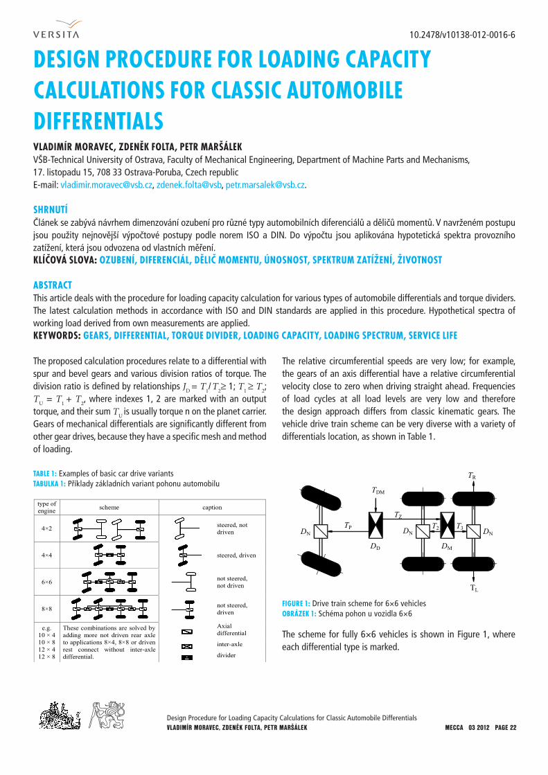
The proposed calculation procedures relate to a differential with spur and bevel gears and various division ratios of torque. The division ratio is defined by relationships JD = T1/ T2≥ 1; T1 ≥ T2; TU = T1 + T2, where indexes 1, 2 are marked with an output torque, and their sum TU is usually torque n on the planet carrier. Gears of mechanical differentials are significantly different from other gear drives, because they have a specific mesh and method of loading.

The relative circumferential speeds are very low; for example, the gears of an axis differential have a relative circumferential velocity close to zero when driving straight ahead. Frequencies of load cycles at all load levels are very low and therefore the design approach differs from classic kinematic gears. The vehicle drive train scheme can be very diverse with a variety of differentials location, as shown in Table 1.

The scheme for fully 6×6 vehicles is shown in Figure 1, where each differential type is marked.

VLADIMÍR MORAVEC, ZDENĚK FOLTA, PETR MARŠÁLEKVŠB-Technical University of Ostrava, Faculty of Mechanical Engineering, Department of Machine Parts and Mechanisms, 17. listopadu 15, 708 33 Ostrava-Poruba, Czech republicE-mail: [email protected], zdenek.folta@vsb, [email protected].

SHRNUTÍČlánek se zabývá návrhem dimenzování ozubení pro různé typy automobilních diferenciálů a děličů momentů. V navrženém postupu jsou použity nejnovější výpočtové postupy podle norem ISO a DIN. Do výpočtu jsou aplikována hypotetická spektra provozního zatížení, která jsou odvozena od vlastních měření.KLÍČOVÁ SLOVA: OZUBENÍ, DIFERENCIÁL, DĚLIČ MOMENTU, ÚNOSNOST, SPEKTRUM ZATÍŽENÍ, ŽIVOTNOST

ABSTRACTThis article deals with the procedure for loading capacity calculation for various types of automobile differentials and torque dividers. The latest calculation methods in accordance with ISO and DIN standards are applied in this procedure. Hypothetical spectra of working load derived from own measurements are applied.KEYWORDS: GEARS, DIFFERENTIAL, TORQUE DIVIDER, LOADING CAPACITY, LOADING SPECTRUM, SERVICE LIFE

DESIGN PROCEDURE FOR LOADING CAPACITY CALCULATIONS FOR CLASSIC AUTOMOBILE DIFFERENTIALS

TABLE 1: Examples of basic car drive variants TABULKA 1: Příklady základních variant pohonu automobilu

FIGURE 1: Drive train scheme for 6×6 vehicles OBRÁZEK 1: Schéma pohon u vozidla 6×6

Design Procedure for Loading Capacity Calculations for Classic Automobile DifferentialsVLAdIMíR MORAVEC, ZdENěK FOLTA, PETR MARšáLEK MECCA 03 2012 PAGE 23MECCA 03 2012 PAGE 22

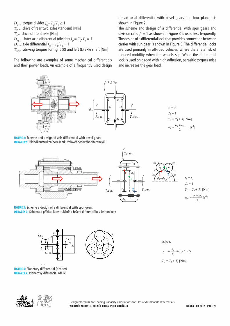
DD…torque divider JD=TZ/TP ≥ 1TZ …drive of rear two axles (tandem) [Nm]TP…drive of front axle [Nm]DM …inter-axle differential (divider) JD = T2/T3 = 1DN…axle differential JD = TR/TL = 1TR,L…driving torques for right (R) and left (L) axle shaft [Nm]

The following are examples of some mechanical differentials and their power loads. An example of a frequently used design

for an axial differential with bevel gears and four planets is shown in Figure 2.The scheme and design of a differential with spur gears and division ratio JD = 1 as shown in Figure 3 is used less frequently. The design of a differential lock that provides connection between carrier with sun gear is shown in Figure 3. The differential locks are used primarily in off-road vehicles, where there is a risk of reduced mobility when the wheels slip. When the differential lock is used on a road with high adhesion, parasitic torques arise and increases the gear load.

FIGURE 2: Scheme and design of axis differential with bevel gearsOBRÁZEK2:Příkladkonstrukčníhořešeníkuželovéhoosovéhodiferenciálu

FIGURE 3: Scheme a design of a differential with spur gearsOBRÁZEK 3: Schéma a příklad konstrukčního řešení diferenciálu s čelnímikoly

FIGURE 4: Planetary differential (divider)OBRÁZEK 4: Planetový diferenciál (dělič)


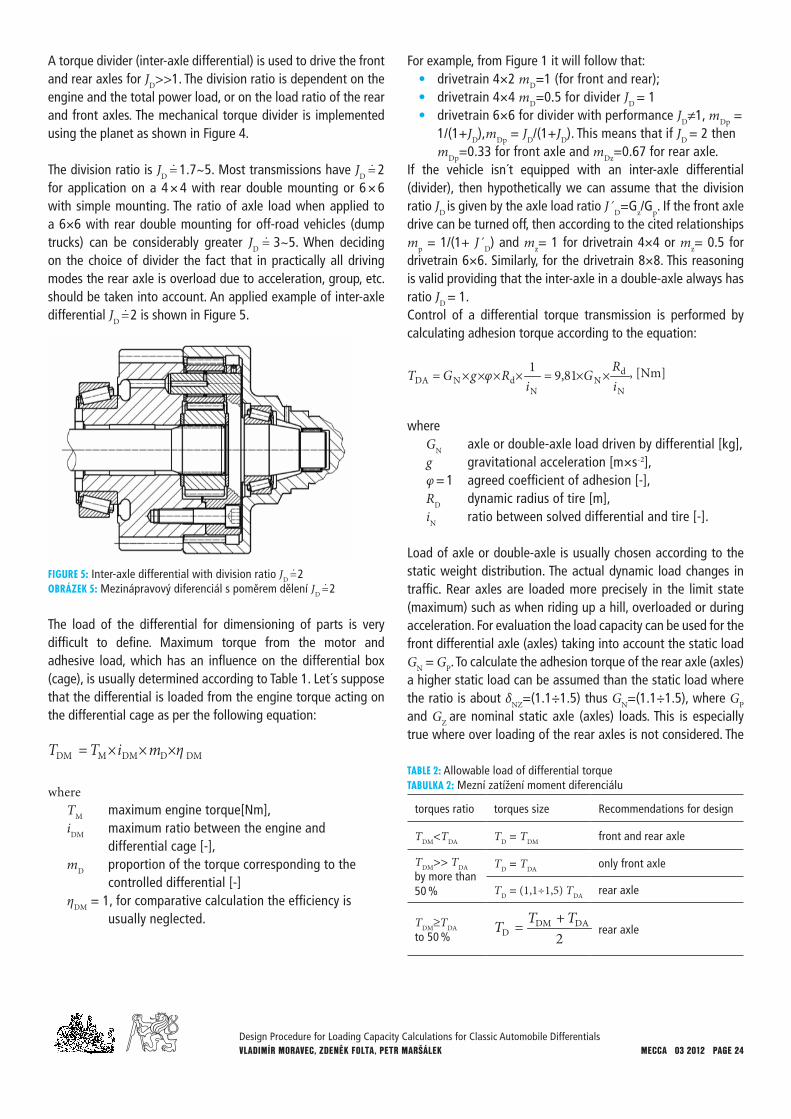
A torque divider (inter-axle differential) is used to drive the front and rear axles for JD>>1. The division ratio is dependent on the engine and the total power load, or on the load ratio of the rear and front axles. The mechanical torque divider is implemented using the planet as shown in Figure 4.

The division ratio is JD =. 1.7~5. Most transmissions have JD =. 2 for application on a 4 × 4 with rear double mounting or 6 × 6 with simple mounting. The ratio of axle load when applied to a 6×6 with rear double mounting for off-road vehicles (dump trucks) can be considerably greater JD =. 3~5. When deciding on the choice of divider the fact that in practically all driving modes the rear axle is overload due to acceleration, group, etc. should be taken into account. An applied example of inter-axle differential JD =. 2 is shown in Figure 5.

FIGURE 5: Inter-axle differential with division ratio JD =. 2OBRÁZEK 5: Mezinápravový diferenciál s poměrem dělení JD =. 2

The load of the differential for dimensioning of parts is very difficult to define. Maximum torque from the motor and adhesive load, which has an influence on the differential box (cage), is usually determined according to Table 1. Let´s suppose that the differential is loaded from the engine torque acting on the differential cage as per the following equation:

DMDDMMDM miTT η×××=

whereTM maximum engine torque[Nm],iDM maximum ratio between the engine and

differential cage [-],mD proportion of the torque corresponding to the

controlled differential [-] ηDM = 1, for comparative calculation the efficiency is

usually neglected.

For example, from Figure 1 it will follow that: • drivetrain 4×2 mD=1 (for front and rear);• drivetrain 4×4 mD=0.5 for divider JD = 1 • drivetrain 6×6 for divider with performance JD≠1, mDp =

1/(1+JD),mDp = JD/(1+JD). This means that if JD = 2 then mDp=0.33 for front axle and mDz=0.67 for rear axle.

If the vehicle isn´t equipped with an inter-axle differential (divider), then hypothetically we can assume that the division ratio JD is given by the axle load ratio J´D=Gz/Gp. If the front axle drive can be turned off, then according to the cited relationships mp = 1/(1+ J´D) and mz= 1 for drivetrain 4×4 or mz= 0.5 for drivetrain 6×6. Similarly, for the drivetrain 8×8. This reasoning is valid providing that the inter-axle in a double-axle always has ratio JD = 1.Control of a differential torque transmission is performed by calculating adhesion torque according to the equation:

N

dN

NdNDA i

RGi

RgGT ××=××××= 81,91φ , [Nm]

whereGN axle or double-axle load driven by differential [kg],g gravitational acceleration [m×s-2],φ = 1 agreed coefficient of adhesion [-],RD dynamic radius of tire [m],iN ratio between solved differential and tire [-].

Load of axle or double-axle is usually chosen according to the static weight distribution. The actual dynamic load changes in traffic. Rear axles are loaded more precisely in the limit state (maximum) such as when riding up a hill, overloaded or during acceleration. For evaluation the load capacity can be used for the front differential axle (axles) taking into account the static load GN = GP. To calculate the adhesion torque of the rear axle (axles) a higher static load can be assumed than the static load where the ratio is about δNZ=(1.1÷1.5) thus GN=(1.1÷1.5), where GP and GZ are nominal static axle (axles) loads. This is especially true where over loading of the rear axles is not considered. The

TABLE 2: Allowable load of differential torque TABULKA 2: Mezní zatížení moment diferenciálu

torques ratio torques size Recommendations for design

TDM<TDA TD = TDM front and rear axle

TDM>> TDAby more than 50 %

TD = TDA only front axle

TD = (1,1÷1,5) TDA rear axle

TDM≥TDAto 50 % 2

DADMD

TTT += rear axle


resulting agreed torques acting on a planet carrier (differential cage) for the comparative strength calculations are summarized for various operating conditions in Table 2. The forces between the teeth of all the differentials are given by the equation:

ndTF×

××= δUT

2000 , [N]

whereTU=TD torque moment on the driving element of

a differential given by Table 2[Nm],n number of planetary gears or pairs of planetary

gears[-],δ degree of inequality of a force distribution

(Table 3)[-],d reference or the pitch diameter of driving element

of a differential [mm].The rotation load of differential gears, such as number of cycles, differs significantly over a variety of vehicle driving conditions.

Rotations of the differential gear are theoretically zero when driving is straight. The spinning of the differential gear occurs under the following conditions:

• driven wheel tires have different rolling radii and different load,

• driven wheels or axles move along an unequal length of the roadway (curves, transverse and longitudinal irregularities),

• uneven traction of tires on one axle (or axles for inter-axle differentials) due to uneven adhesion or different characteristics of tire slip.

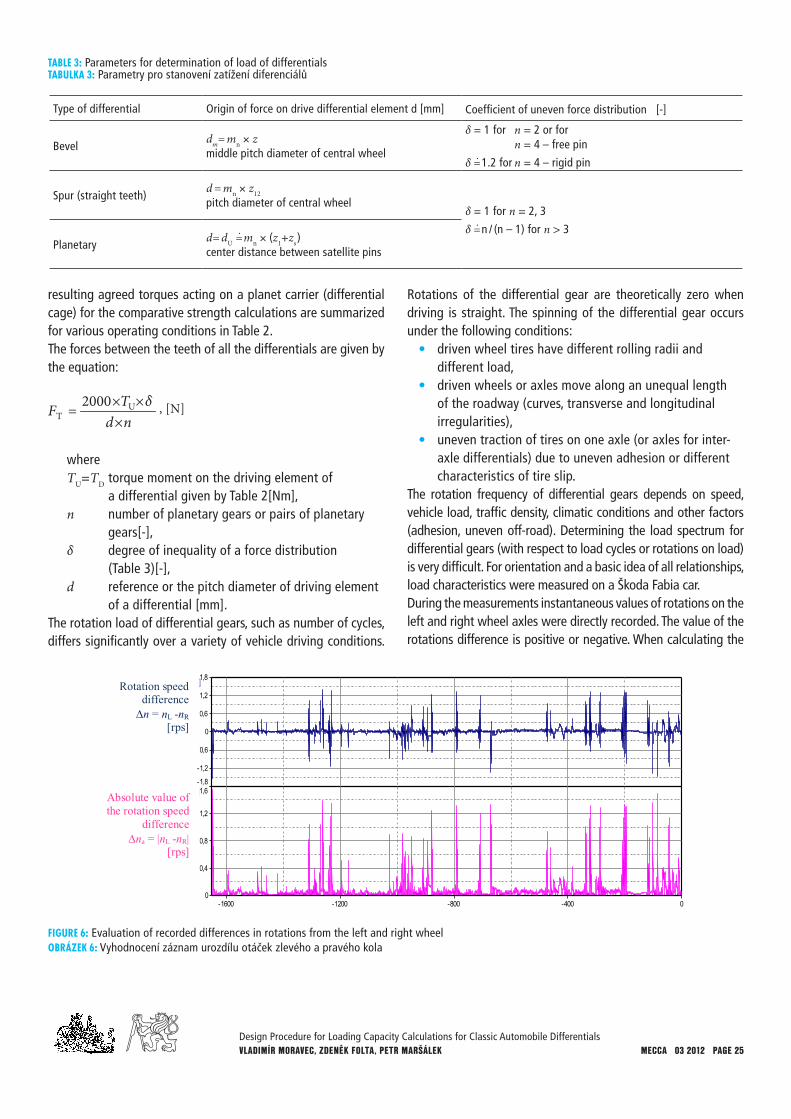
The rotation frequency of differential gears depends on speed, vehicle load, traffic density, climatic conditions and other factors (adhesion, uneven off-road). Determining the load spectrum for differential gears (with respect to load cycles or rotations on load) is very difficult. For orientation and a basic idea of all relationships, load characteristics were measured on a Škoda Fabia car. During the measurements instantaneous values of rotations on the left and right wheel axles were directly recorded. The value of the rotations difference is positive or negative. When calculating the

FIGURE 6: Evaluation of recorded differences in rotations from the left and right wheelOBRÁZEK 6: Vyhodnocení záznam urozdílu otáček zlevého a pravého kola

TABLE 3: Parameters for determination of load of differentialsTABULKA 3: Parametry pro stanovení zatížení diferenciálů

Type of differential Origin of force on drive differential element d [mm] Coefficient of uneven force distribution δ [-]

Beveldm= mn × z middle pitch diameter of central wheel

δ = 1 for n = 2 or for n = 4 – free pin

δ =. 1.2 for n = 4 – rigid pin

Spur (straight teeth) d = mn × z12pitch diameter of central wheel

δ = 1 for n = 2, 3

δ =. n / (n – 1) for n > 3Planetary

d= dU =. mn × (z1+zs )center distance between satellite pins


differential loads, differences in the absolute value of the rotation difference between the left and the right half axle: ∆na = |nL - nR| are also taken into account.An example of difference and frequency of rotations of automobile wheels during city driving is shown in Figure 6.

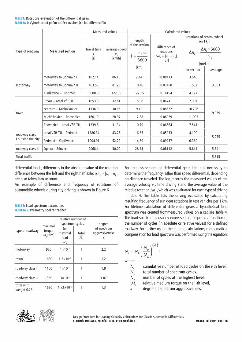
For the assessment of differential gear life it is necessary to determine the frequency rather than speed differential, depending on distance traveled. The log records the measured values of the average velocity vp, time driving t and the average value of the relative rotation ∆na , which was evaluated for each type of driving in Table 4. This Table lists the driving evaluated by calculating resulting frequency of sun gear rotations in test vehicles per 1 km.For lifetime calculation of differential gears a hypothetical load spectrum was created from measured values on a car, see Table 4. The load spectrum is usually expressed as torque as a function of the number of cycles (in absolute or relative values) for a defined roadway. For further use in the lifetime calculations, mathematical compensation for load spectrum was performed using the equation:

( )sM

NN

NNi

C

pCi = ⎟

⎠

⎞⎜⎝

⎛ ,

whereNi cumulative number of load cycles on the i-th level,NC total number of spectrum cycles,NP number of cycles at the highest level,—Mi relative medium torque on the i-th level,s degree of spectrum aggressiveness.

TABLE 4: Rotations evaluation of the differential gears TABULKA 4: Vyhodnocení počtu otáček ozubených kol diferenciálu

Type of roadway Measured section

Measured values Calculated values

travel timet

[s]

average speedvp

[km/h]

length of the section

3600tv

l p×=

[km]

difference of rotations

∆na = |nL – nR|[s-1]

rotations of central wheel on 1 km

p

ai v

nn 3600×Δ=Δ

[rot/km]

in section average

motorway

motorway to Bohumín I 102.14 86.16 2.44 0.08473 3.540

3.083motorway to Bohumín II 463.58 81.23 10.46 0.03458 1.532

Klimkovice – Pustiměř 3600.0 122.35 122.35 0.14194 4.177

town

Přívoz – areal VŠB-TU 1653.0 32.81 15.06 0.06741 7.397

9.059centrum – Michálkovice 1136.0 30.06 9.49 0.08522 10.206

Michálkovice – Radvanice 1601.0 28.97 12.88 0.08929 11.093

Radvanice – areal VŠB-TU 1239.6 31.34 10.79 0.06564 7.541

roadway class I outside the city

areal VŠB-TU – Petřvald 1386.34 43.25 16.65 0.05033 4.1905.275

Petřvald – Kopřivnice 1004.91 52.29 14.60 0.09237 6.360

roadway class II Opava – Bílovec 2068.4 50.00 28.73 0.08112 5.841 5.841

Total traffic 5.815

TABLE 5: Load spectrum parametersTABULKA 5: Parametry spekter zatížení

type of roadwaymaximaltorque

MP[Nm]

relative number of spectrum cycles degree

of spectrum aggressiveness

s

for maximal

load—NP

total—NC

motorway 970 1×10-3 1 2.2

town 1650 1.2×10-5 1 1.2

roadway class I 1150 1×10-5 1 1.9

roadway class II 1350 3×10-4 1 1.07

total with weight 0.25

1620 1.72×10-6 1 1.3


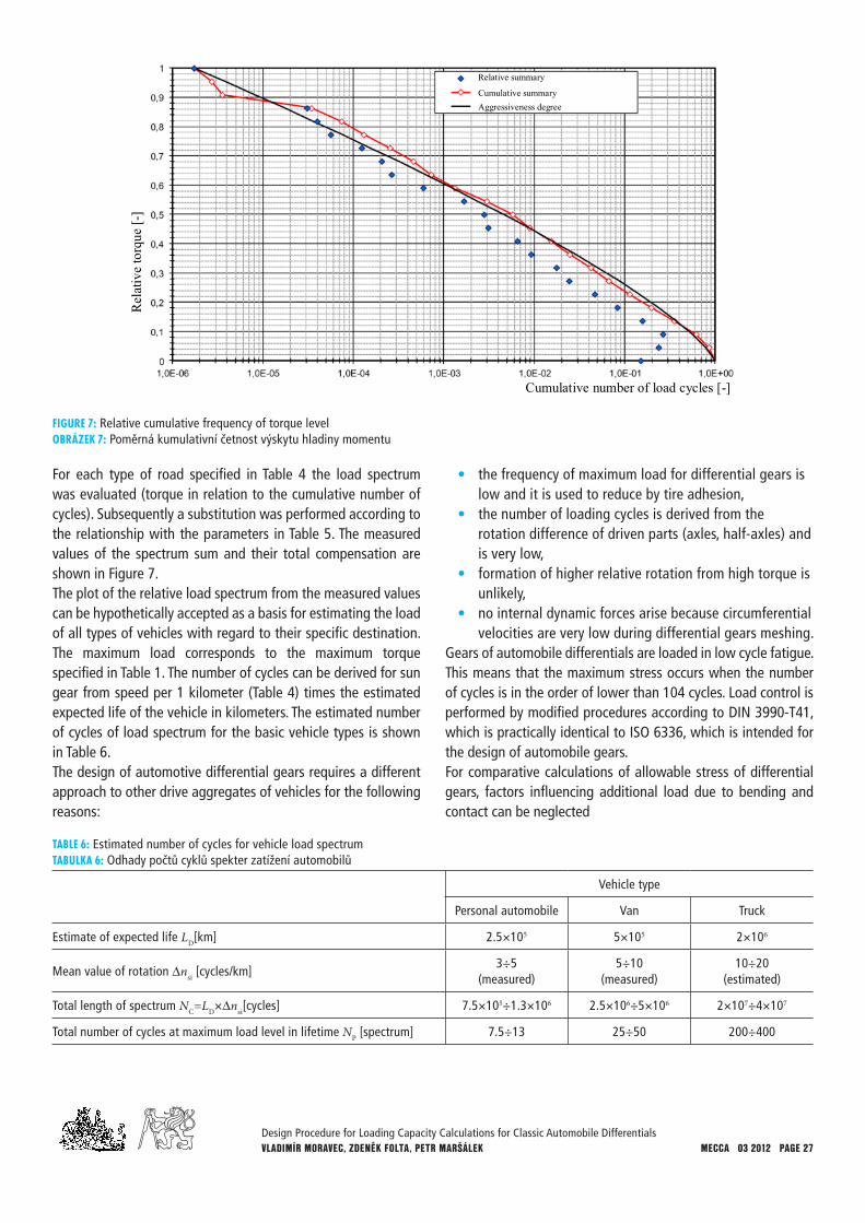
For each type of road specified in Table 4 the load spectrum was evaluated (torque in relation to the cumulative number of cycles). Subsequently a substitution was performed according to the relationship with the parameters in Table 5. The measured values of the spectrum sum and their total compensation are shown in Figure 7. The plot of the relative load spectrum from the measured values can be hypothetically accepted as a basis for estimating the load of all types of vehicles with regard to their specific destination. The maximum load corresponds to the maximum torque specified in Table 1. The number of cycles can be derived for sun gear from speed per 1 kilometer (Table 4) times the estimated expected life of the vehicle in kilometers. The estimated number of cycles of load spectrum for the basic vehicle types is shown in Table 6.The design of automotive differential gears requires a different approach to other drive aggregates of vehicles for the following reasons:

• the frequency of maximum load for differential gears is low and it is used to reduce by tire adhesion,

• the number of loading cycles is derived from the rotation difference of driven parts (axles, half-axles) and is very low,

• formation of higher relative rotation from high torque is unlikely,

• no internal dynamic forces arise because circumferential velocities are very low during differential gears meshing.

Gears of automobile differentials are loaded in low cycle fatigue. This means that the maximum stress occurs when the number of cycles is in the order of lower than 104 cycles. Load control is performed by modified procedures according to DIN 3990-T41, which is practically identical to ISO 6336, which is intended for the design of automobile gears.For comparative calculations of allowable stress of differential gears, factors influencing additional load due to bending and contact can be neglected

TABLE 6: Estimated number of cycles for vehicle load spectrumTABULKA 6: Odhady počtů cyklů spekter zatížení automobilů

Vehicle type

Personal automobile Van Truck

Estimate of expected life LD[km] 2.5×105 5×105 2×106

Mean value of rotation ∆nsi [cycles/km]3÷5

(measured)5÷10

(measured)10÷20

(estimated)

Total length of spectrum NC=LD×∆nsi[cycles] 7.5×105÷1.3×106 2.5×106÷5×106 2×107÷4×107

Total number of cycles at maximum load level in lifetime NP [spectrum] 7.5÷13 25÷50 200÷400

FIGURE 7: Relative cumulative frequency of torque levelOBRÁZEK 7: Poměrná kumulativní četnost výskytu hladiny momentu


KF = KA×KFv×KFβ = KFα = KH = KA×KHv×KHβ×KHα = 1

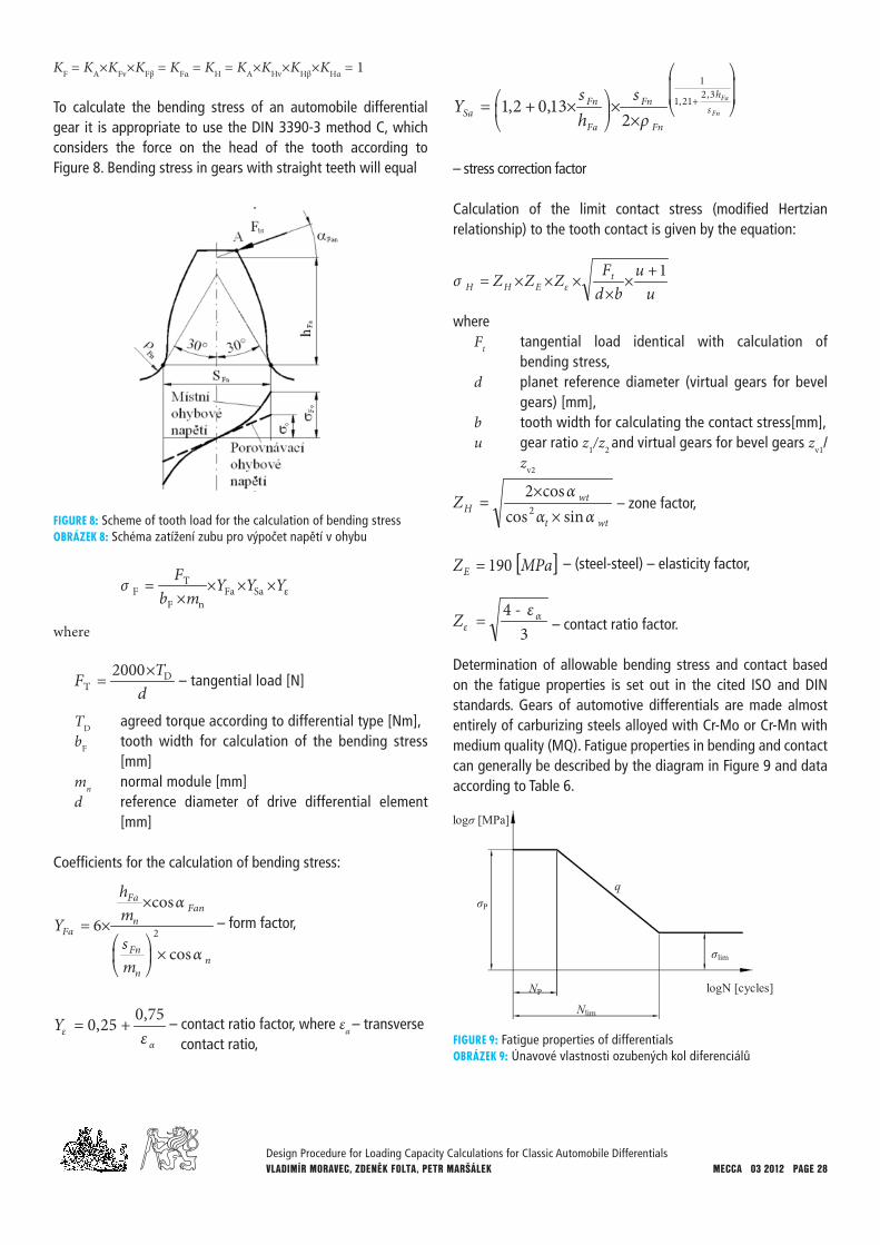
To calculate the bending stress of an automobile differential gear it is appropriate to use the DIN 3390-3 method C, which considers the force on the head of the tooth according to Figure 8. Bending stress in gears with straight teeth will equal

FIGURE 8: Scheme of tooth load for the calculation of bending stressOBRÁZEK 8: Schéma zatížení zubu pro výpočet napětí v ohybu

εSaFaT

F YYYmb

FnF

××××

=σ

where

dTF D

T2000×= – tangential load [N]

TD agreed torque according to differential type [Nm],bF tooth width for calculation of the bending stress

[mm]mn normal module [mm]d reference diameter of drive differential element

[mm]

Coefficients for the calculation of bending stress:

nn

Fn

Fann

Fa

Fa

ms

mh

Y

α

α

cos

cos6 2

×

××=

⎟⎠

⎞⎜⎝

⎛ – form factor,

αε ε

75,025,0 +=Y – contact ratio factor, where εα – transverse contact ratio,

+

×××+= Fn

Fash

Fn

Fn

Fa

FnSa

shsY

3,221,1

1

213,02,1

ρ⎟⎠

⎞⎜⎝

⎛ ⎟⎠

⎞⎜⎝

⎛

– stress correction factor

Calculation of the limit contact stress (modified Hertzian relationship) to the tooth contact is given by the equation:

uu

bdFZZZ t

EHH1+×

××××= εσ

whereFt tangential load identical with calculation of

bending stress,d planet reference diameter (virtual gears for bevel

gears) [mm],b tooth width for calculating the contact stress[mm],u gear ratio z1/z2 and virtual gears for bevel gears zv1/

zv2

wtt

wtHZ αα

αsincos

cos22 ××= – zone factor,

[ ]MPaZE 190= – (steel-steel) – elasticity factor,

34 α

εε-=Z – contact ratio factor.

Determination of allowable bending stress and contact based on the fatigue properties is set out in the cited ISO and DIN standards. Gears of automotive differentials are made almost entirely of carburizing steels alloyed with Cr-Mo or Cr-Mn with medium quality (MQ). Fatigue properties in bending and contact can generally be described by the diagram in Figure 9 and data according to Table 6.

FIGURE 9: Fatigue properties of differentials OBRÁZEK 9: Únavové vlastnosti ozubených kol diferenciálů


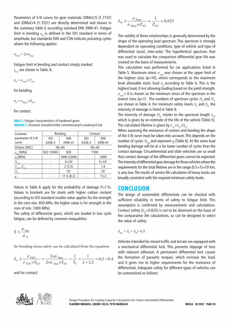
Parameters of S-N curves for gear materials 20MnCr5 (1.7147) and 20MoCr4 (1.7321) are directly determined and shown in the summary Table 6 according standard DIN 3990-41. Fatigue limit in bending sFE is defined in the ISO standard in terms of amplitude, but standards DIN and ČSN indicate pulsating cycles where the following applies:

σFEN = 2×σFlim

Fatigue limit in bending and contact simply marked slim are shown in Table. 6.

σP = σFEN×YNT

for bending,

σP = σHlim×ZNT

for contact.

TABLE 7: Fatigue characteristics of hardened gearsTABULKA 7: Únavové charakteristiky cementovaných ozubených kol

Common parameter of S-N curve

Bending ContactISO

6336-5DIN

3990-41ISO

6336-5DIN

3990-41Vickers [HRC] 58÷64 58÷64σlim[MPa] 922 (1000) 920 1500σP[MPa] - 1840 (2300) - 2400Nlim - 3×106 - 5×107

YNT, ZNT - 2 (2.5) - 1.6NP - 103 - 105

q - 11.5 (8.3) - 13.2

Values in Table 6 apply for the probability of damage P=1 %. Values in brackets are for steels with higher carbon content (according to ISO standard smaller value applies for the strength in the core min. 850 MPa, the higher value is for strength in the core of min. 1000 MPa).The safety of differential gears, which are loaded in low cycle fatigue, can be defined by common inequalities:

P

lim

σσ≤S

for bending stress safety can be calculated from the equation:

4,05,05,22

112

2FNTFlim

Flim

NTFEN

FENF ÷=

÷==

×××=

×≤

YYYS

σσ

σσ

and for contact:

625,01

NTNTHlim

HlimH ==

×≤

ZZS

σσ

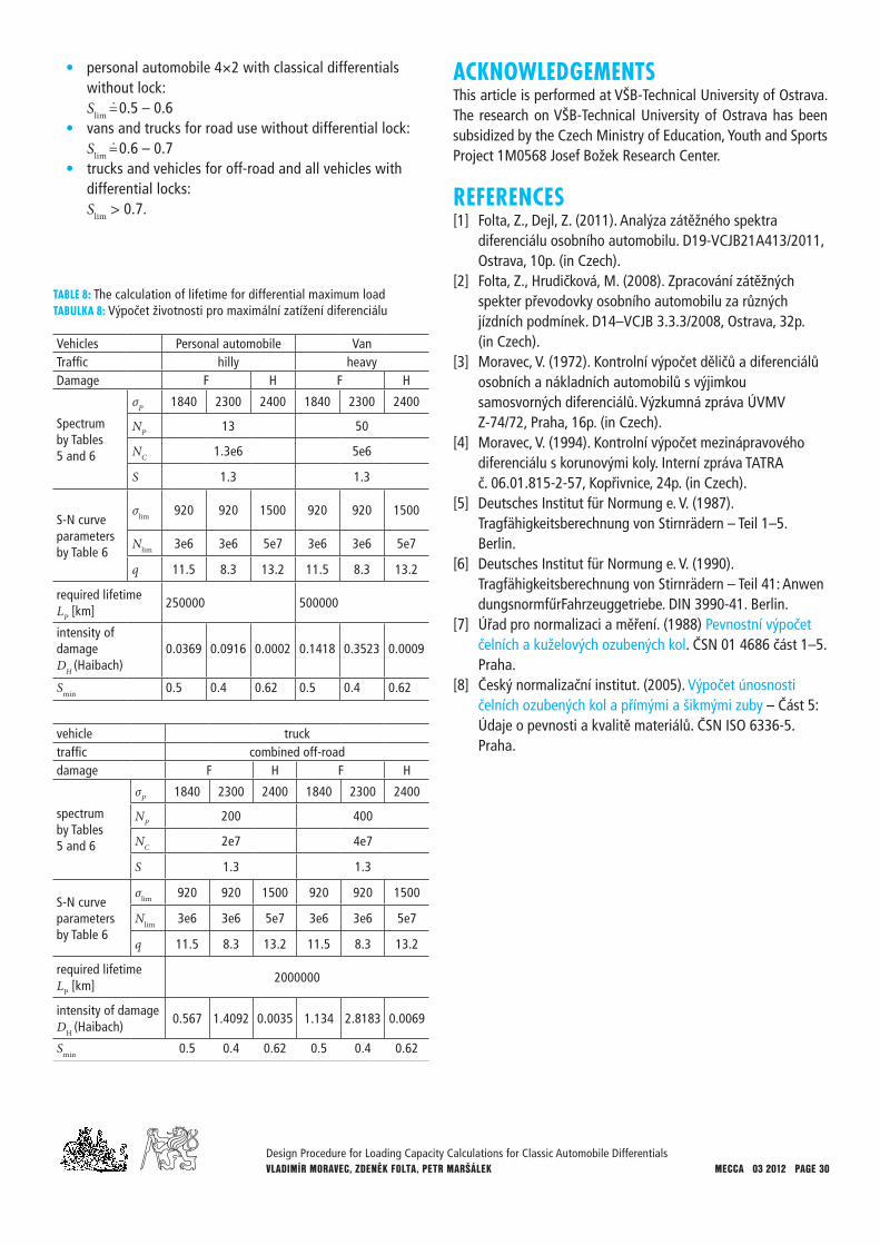
The validity of these relationships is generally determined by the shape of the operating load spectrum. This spectrum is strongly dependent on operating conditions, type of vehicle and type of differential (axial, inter-axle). The hypothetical spectrum that was used to calculate the comparison differential gear life was created on the basis of measurements.This calculation was performed for car applications listed in Table 5. Maximum stress σmax was chosen at the upper limit of the highest class (p=10), which corresponds to the maximum level allowable static load σp according to Table 6. This is the highest load, if not allowing loading based on the yield strength. σmin= 0 is chosen as the minimum stress of the spectrum in the lowest class (p=1) . The numbers of spectrum cycles NP and NC are shown in Table 4. For minimum safety levels SF and SH the intensity of damage is listed in Table 8.The intensity of damage DH relates to the spectrum length LP, which is given by an estimate of the life of the vehicle (Table 5). The calculated lifetime is given by Lzv=LP/DH.When assessing the resistance of contact and bending the shape of the S-N curve must be taken into account. This depends on the number of cycles Nlim and exponent q (Table 6). At the same load bending damage will be at a far lower number of cycles than the contact damage. Circumferential and slide velocities are so small that contact damage of the differential gears cannot be expected. The intensity of differential gear damage for those vehicles where the requirements for the total lifetime are in the range (0.5÷1)×106 km, is very low. The results of service life calculation of heavy trucks are broadly consistent with the required minimum safety levels.

CONCLUSIONThe design of automobile differentials can be checked with sufficient reliability in terms of safety to fatigue limit. This assumption is confirmed by measurements and calculations. Contact safety (SH<0.625) is not to be observed on the basis of the comparative life calculations, so can be designed to select the value of safety:

Slim = SF = SH> 0.5

Vehicles intended for mixed traffic and terrain are equipped with a mechanical differential lock. This prevents slippage of tires with reduced adhesion. A permanent differential lock causes the formation of parasitic torques, which increase the load, and it gives rise to higher requirements for the resistance of differentials. Adequate safety for different types of vehicles can be summarized as follows:

MECCA 03 2012 PAGE 30Design Procedure for Loading Capacity Calculations for Classic Automobile DifferentialsVLAdIMíR MORAVEC, ZdENěK FOLTA, PETR MARšáLEK

• personal automobile 4×2 with classical differentials without lock: Slim =. 0.5 – 0.6

• vans and trucks for road use without differential lock: Slim =. 0.6 – 0.7

• trucks and vehicles for off-road and all vehicles with differential locks: Slim > 0.7.

ACKNOWLEDGEMENTSThis article is performed at VŠB-Technical University of Ostrava. The research on VŠB-Technical University of Ostrava has been subsidized by the Czech Ministry of Education, Youth and Sports Project 1M0568 Josef Božek Research Center.

REFERENCES[1] Folta, Z., Dejl, Z. (2011). Analýza zátěžného spektra

diferenciálu osobního automobilu. D19-VCJB21A413/2011, Ostrava, 10p. (in Czech).

[2] Folta, Z., Hrudičková, M. (2008). Zpracování zátěžných spekter převodovky osobního automobilu za různých jízdních podmínek. D14–VCJB 3.3.3/2008, Ostrava, 32p. (in Czech).

[3] Moravec, V. (1972). Kontrolní výpočet děličů a diferenciálů osobních a nákladních automobilů s výjimkou samosvorných diferenciálů. Výzkumná zpráva ÚVMV Z-74/72, Praha, 16p. (in Czech).

[4] Moravec, V. (1994). Kontrolní výpočet mezinápravového diferenciálu s korunovými koly. Interní zpráva TATRA č. 06.01.815-2-57, Kopřivnice, 24p. (in Czech).

[5] Deutsches Institut für Normung e. V. (1987). Tragfähigkeitsberechnung von Stirnrädern – Teil 1–5. Berlin.

[6] Deutsches Institut für Normung e. V. (1990). Tragfähigkeitsberechnung von Stirnrädern – Teil 41: AnwendungsnormfűrFahrzeuggetriebe. DIN 3990-41. Berlin.

[7] Úřad pro normalizaci a měření. (1988) Pevnostní výpočet čelních a kuželových ozubených kol. ČSN 01 4686 část 1–5. Praha.

[8] Český normalizační institut. (2005). Výpočet únosnosti čelních ozubených kol a přímými a šikmými zuby – Část 5: Údaje o pevnosti a kvalitě materiálů. ČSN ISO 6336-5. Praha.

TABLE 8: The calculation of lifetime for differential maximum loadTABULKA 8: Výpočet životnosti pro maximální zatížení diferenciálu

Vehicles Personal automobile VanTraffic hilly heavyDamage F H F H

Spectrumby Tables5 and 6

σP 1840 2300 2400 1840 2300 2400

NP 13 50

NC 1.3e6 5e6

S 1.3 1.3

S-N curveparametersby Table 6

σlim 920 920 1500 920 920 1500

Nlim 3e6 3e6 5e7 3e6 3e6 5e7

q 11.5 8.3 13.2 11.5 8.3 13.2

required lifetimeLP [km]

250000 500000

intensity of damageDH (Haibach)

0.0369 0.0916 0.0002 0.1418 0.3523 0.0009

Smin 0.5 0.4 0.62 0.5 0.4 0.62

vehicle trucktraffic combined off-roaddamage F H F H

spectrumby Tables 5 and 6

σP 1840 2300 2400 1840 2300 2400

NP 200 400

NC 2e7 4e7

S 1.3 1.3

S-N curveparametersby Table 6

σlim 920 920 1500 920 920 1500

Nlim 3e6 3e6 5e7 3e6 3e6 5e7

q 11.5 8.3 13.2 11.5 8.3 13.2

required lifetimeLP [km]

2000000

intensity of damageDH (Haibach)

0.567 1.4092 0.0035 1.134 2.8183 0.0069

Smin 0.5 0.4 0.62 0.5 0.4 0.62

design procedure for loading capacity calculations for classic ...

Documents