Design of the simulation platform for networked control systems based on DTHMM

Proceedings of the 8th

World Congress on Intelligent Control and Automation July 6-9 2010, Jinan, China

978-1-4244-6712-9/10/$26.00 ©2010 IEEE

Design of the Simulation Platform for Networked Control Systems Based on DTHMM*

Yuan Ge1,2, Shuang Cong1, Qigong Chen2, Ming Jiang2 and Weiwei Shang1 1.Department of Automation, University of Science and Technology of China, Hefei, Anhui Province, China

2. Department of Electrical Engineering, Anhui University of Technology and Science, Wuhu, Anhui Province, China [email protected], Corresponding author: [email protected], [email protected]

* This work is partially supported by the National Science Foundation of China (60774098, 60843003, 50905172), the Science Foundation of Anhui Province (090412071, 090412040), and the University of Science and Technology of China Initiative Foundation.

Abstract - In order to achieve the application of discrete-time hidden Markov model (DTHMM) in modeling and controlling the networked control system (NCS) with the network-induced delays in the forward channel, a simulation platform was designed and implemented in this paper by using TrueTime 1.5, which is a Matlab/Simulink-based simulator. There were one network module and four kernel modules (sensor, controller, actuator and interference nodes) on this simulation platform, and the composition and the main Matlab codes of each module were presented. On the simulation platform designed, the Expectation Maximization (EM) algorithm was achieved to derive the parameters of the DTHMM and the Viterbi algorithm was achieved to predict the controller-to-actuator delay (C-A delay) in the current sampling period. Based on the derived DTHMM and the predicted delays, a state-feedback controller to stabilize the NCS was also implemented on the simulation platform and used to solve the linear matrix inequalities. Taking a damped compound pendulum as the plant in the NCS, after 500 sampling periods the effectiveness of the modeling and controlling methods was carried out, and demonstrated the efficiency and easy operation of the simulation platform.

Index Terms – Networked control system. Discrete-time hidden Markov model. Simulation platform. TrueTime. Linear matrix inequality.

I. INTRODUCTION

Recently, real-time networks are integrated into control systems to form networked control systems (NCSs) wherein the information of system components (sensors, controller, actuators, etc.) is exchanged via networks [1-3]. The main advantages of NCSs are reduced system wiring, ease of system maintenance, and improved system flexibility. The networked control architecture has been adopted in a broad range of areas such as remote surgery, manufacturing automation, and automated highway systems. However, the insertion of the network in the feedback control loop raises new problems such as the network-induced delays. These delays, either constant or time varying, degrade the system performance and even cause the system instability, which makes the analysis and design of the NCS complex. Over the past several years, considerable attention has been devoted to the research on modeling, stability analysis and controller design for NCSs in the presence of network-induced delays. The properties of the network-induced delays in a general NCS were described in [4]. The stability analyses of the NCS with delays were presented in [5-6], and the

controller design methods of the NCS with delays were proposed in [7-8]. Moreover, when the random delays have Markovian characteristic, the NCS can be formulated as a Markovian jump linear system (MJLS). Based on the theories of the MJLS, many results about the stability analysis and the controller design of the NCS can be found in [9-10]. While using Markov chains to model the delays in an NCS, we noticed that in the aforementioned two papers, the state transition matrix was assumed to be known in advance. However, this kind of assumption is too ideal to agree with the real situation. Actually, the network-induced delays are some kind of network QoS (Quality of Service) that reflects the state of network. As an abstract variable, the network state can not be well defined but can be perceived by an application only through its effects on its packet flow such as network-induced delays. By treating the network states as a hidden Markov chain and the network-induced delays as a set of observations, the LQG optimal controller for the NCS with delays was presented in [11]. Following the same line as in [11], a mode-dependent state feedback controller was derived to guarantee the stochastic stability for an uncertain NCS [12], and a mode-dependent output feedback controller was derived to achieve both robust stability and prescribed disturbance attenuation performance for an uncertain NCS [13]. Furthermore, the Baum-Welch algorithm was used to derive the parameters of the hidden Markov model (HMM) for the NCS with delays, where the state transition matrices of the Markov chain could be derived online without the ideal assumption that they are known in advance [14-16]. To the best of authors’ knowledge, the modeling method and the controller design for an NCS based on the HMM has become a hot topic of the NCS research although it is still in its infant stage. In order to facilitate this research, a simulation platform is necessary to demonstrate the effectiveness of these modeling and controller designing methods for NCSs based on the HMM. At present, lots of work on the simulation of the NCS has been conducted [17-19], where TrueTime, as a Matlab/Simulink-based simulator for the networked and embedded control systems developed at Lund University, are more widely accepted since it is more powerful and simpler in the field of the NCS simulation compared with other simulators.

4400

In this paper, based on TrueTime 1.5 we design the simulation platform for the NCS with delays when applying the DTHMM to the modeling and the controller design for this system. On this simulation platform, there are six main modules including a plant, a time-driven sensor, an event-driven controller, an event-driven actuator, an interference node and the network. The DTHMM is used to describe the relationship between the network states and the network-induced delays, and the EM algorithm is proposed to derive the parameters of this DTHMM. Based on the derived DTHMM and the Viterbi algorithm, the prediction of the C-A delays is achieved. Based on the predicted delays and the derived DTHMM, the NCS is modeled as a MJLS and a state-feedback controller is designed to guarantee the stability of the NCS. The DTHMM derivation, the delay prediction, and the controller design are all achieved at the controller node and verified on this simulation platform. Some structure blocks and flow diagrams are given to represent the construction and the workflow of the simulation platform, and some simulation results are given to demonstrate the effectiveness of the simulation platform. The remainder of this paper is organized as follows. Section 2 carries out the simulation platform based on TrueTime 1.5 and presents the composition and the main codes of each module. In Section 3, the derivation of the DTHMM based on the EM algorithm and the prediction of the current C-A delay based on the Viterbi algorithm are achieved on this simulation platform. Section 4 presents the state-feedback controller designed on this simulation platform by modeling the NCS as a discrete-time MJLS and solving the linear matrix inequalities. Finally, the conclusions are given in Section 5.

II. DESIGN OF THE SIMULATION PLATFORM BASED ON TRUETIME 1.5

As a Matlab/Simulink-based simulator, TrueTime 1.5 consists of a Simulink block library and a collection of MEX files. In the block library, there are six blocks including TrueTime Battery, ttSendMSg, ttGetMsg, TrueTime Wireless Network, TrueTime Network, and TrueTime Kernel, where the last two blocks are used in this paper. The kernel block simulates a computer node with a generic real-time kernel, A/D and D/A converters, and network interfaces. The network block simulates the physical layer and the medium-access layer of various networks. More details about these two blocks can be learned in the reference manual of TrueTime 1.5 [20]. In an NCS, the network-induced delays mainly consist of the sensor-to-controller delay (S-C delay) and the C-A delay as shown in Fig. 1, where the S-C delay and the C-A delay are denoted by sc

kτ and cakτ respectively. Generally, the S-C delay

and the C-A delay have different natures. The S-C delay can be known when the controller uses the plant measurement to calculate the control law, provided that the sensor and the controller are clock-synchronized and the measurement is time stamped before transmission. The C-A delay is different, however, in that it is unknown to the controller at the same time because it has not happened.

actuator plant sensor

network network

controllerforward channel backward channel

xk

uk

cak-1 , ..., , , ,...ca

k-2ca1{ } { sc

1 ,sck-2

sck-1 ,

sck }

Fig. 1 Delays in a general NCS.

If the C-A delay could be predicted before the control law is calculated, both the S-C delay and the C-A delay can be compensated in the control law. Since only the C-A delay needs to be predicted, it is assumed that the network only exists between the controller and the actuator. Meanwhile, ca

kτ is written as kτ for simplicity. Considering that the plant is a damped compound pendulum with the following state space model [21].

x Ax Buy Cx Du

= +⎧⎨ = +⎩

(1)

where 2x ∈ is the state, u ∈ is the control input, and y ∈ is the plant output. The coefficient matrices A , B , C , D are given as follows.

0 110.77 0.039

A⎛ ⎞

= ⎜ ⎟− −⎝ ⎠,

01.89

B⎛ ⎞

= ⎜ ⎟⎝ ⎠

, ( )1 0C = , 0D = .

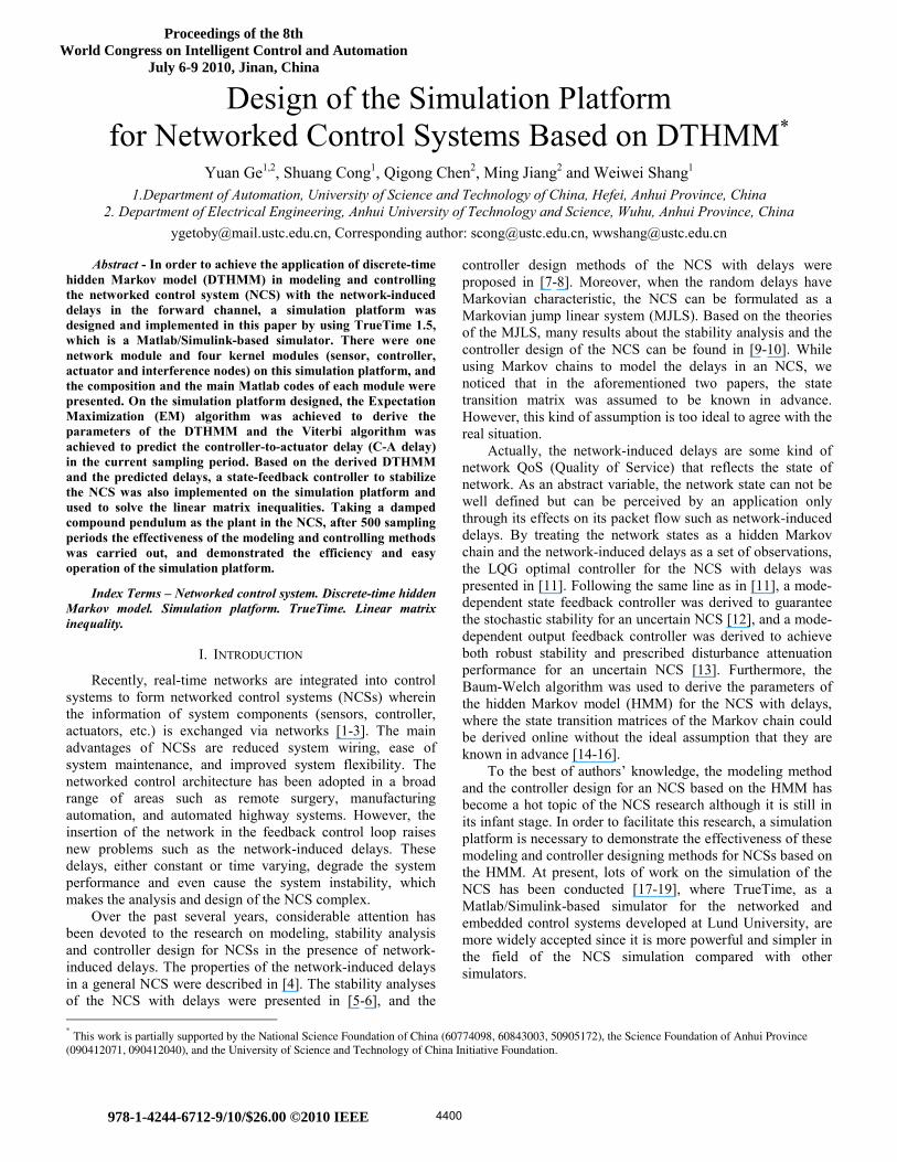
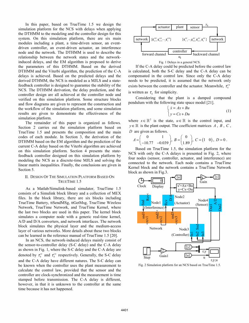
Based on TrueTime 1.5, the simulation platform for the NCS with only the C-A delays is presented in Fig. 2, where four nodes (sensor, controller, actuator, and interference) are connected to the network. Each node contains a TrueTime Kernel block and the network contains a TrueTime Network block as shown in Fig.3.

rcv1sn

d1

rcv2sn

d2

rcv3sn

d3

Network

Rcv

Snd

Rcv D

/A

In1

Snd

In2

In3

A/D

Out

1

Out

2

r,y

uGain12

[y]

[u]r,y;u

kGain

[y][u]

x'=Ax+Buy=Cx+Du

Clock0

Display

Step

Node1(Interference)

Node2

(Actuator)Node4

(Sensor)

Node3(Controller)

Fig. 2 Simulation platform for an NCS based on TrueTime 1.5.

4401

A/DInterruptsRcv

D/ASnd

ScheduleMonitors

PTrueTime Kernel

Sensor1In du/dt

Derivative

1

2

Schedule

A/DInterruptsRcv

D/ASnd

ScheduleMonitors

PTrueTime Kernel

1

2

3

Out1

Out2

In1

In2

In3

1

Schedule

Snd

Controller

A/DInterruptsRcv

D/ASnd

ScheduleMonitors

PTrueTime Kernel

1Rcv

1

Schedule

Actuator

Out

1Rcv

Interference

1

Schedule

Snd

A/DInterruptsRcv

D/ASnd

ScheduleMonitors

PTrueTime Kernel

SndRcv

Schedule

TrueTime Kernel

1

Network1

2

3

Snd1

Snd2

Snd3

1

2

3

Rcv1

Rcv2

Rcv3Schedule

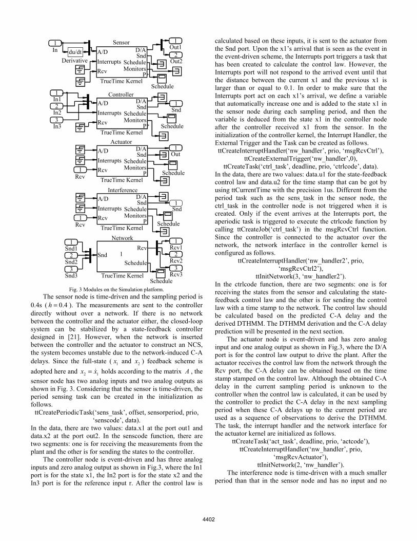
Fig. 3 Modules on the Simulation platform. The sensor node is time-driven and the sampling period is 0.4s ( 0.4h = ). The measurements are sent to the controller directly without over a network. If there is no network between the controller and the actuator either, the closed-loop system can be stabilized by a state-feedback controller designed in [21]. However, when the network is inserted between the controller and the actuator to construct an NCS, the system becomes unstable due to the network-induced C-A delays. Since the full-state ( 1x and 2x ) feedback scheme is adopted here and 2 1x x= holds according to the matrix A , the sensor node has two analog inputs and two analog outputs as shown in Fig. 3. Considering that the sensor is time-driven, the period sensing task can be created in the initialization as follows.

ttCreatePeriodicTask(‘sens_task’, offset, sensorperiod, prio, ‘senscode’, data).

In the data, there are two values: data.x1 at the port out1 and data.x2 at the port out2. In the senscode function, there are two segments: one is for receiving the measurements from the plant and the other is for sending the states to the controller. The controller node is event-driven and has three analog inputs and zero analog output as shown in Fig.3, where the In1 port is for the state x1, the In2 port is for the state x2 and the In3 port is for the reference input r. After the control law is

calculated based on these inputs, it is sent to the actuator from the Snd port. Upon the x1’s arrival that is seen as the event in the event-driven scheme, the Interrupts port triggers a task that has been created to calculate the control law. However, the Interrupts port will not respond to the arrived event until that the distance between the current x1 and the previous x1 is larger than or equal to 0.1. In order to make sure that the Interrupts port act on each x1’s arrival, we define a variable that automatically increase one and is added to the state x1 in the sensor node during each sampling period, and then the variable is deduced from the state x1 in the controller node after the controller received x1 from the sensor. In the initialization of the controller kernel, the Interrupt Handler, the External Trigger and the Task can be created as follows. ttCreateInterruptHandler(‘nw_handler’, prio, ‘msgRcvCtrl’),

ttCreateExternalTrigger(‘nw_handler’,0), ttCreateTask(‘ctrl_task’, deadline, prio, ‘ctrlcode’, data).

In the data, there are two values: data.u1 for the state-feedback control law and data.u2 for the time stamp that can be got by using ttCurrentTime with the precision 1us. Different from the period task such as the sens_task in the sensor node, the ctrl_task in the controller node is not triggered when it is created. Only if the event arrives at the Interrupts port, the aperiodic task is triggered to execute the ctrlcode function by calling ttCreateJob(‘ctrl_task’) in the msgRcvCtrl function. Since the controller is connected to the actuator over the network, the network interface in the controller kernel is configured as follows.

ttCreateInterruptHandler(‘nw_handler2’, prio, ‘msgRcvCtrl2’),

ttInitNetwork(3, ‘nw_handler2’). In the ctrlcode function, there are two segments: one is for receiving the states from the sensor and calculating the state-feedback control law and the other is for sending the control law with a time stamp to the network. The control law should be calculated based on the predicted C-A delay and the derived DTHMM. The DTHMM derivation and the C-A delay prediction will be presented in the next section. The actuator node is event-driven and has zero analog input and one analog output as shown in Fig.3, where the D/A port is for the control law output to drive the plant. After the actuator receives the control law from the network through the Rcv port, the C-A delay can be obtained based on the time stamp stamped on the control law. Although the obtained C-A delay in the current sampling period is unknown to the controller when the control law is calculated, it can be used by the controller to predict the C-A delay in the next sampling period when these C-A delays up to the current period are used as a sequence of observations to derive the DTHMM. The task, the interrupt handler and the network interface for the actuator kernel are initialized as follows.

ttCreateTask(‘act_task’, deadline, prio, ‘actcode’), ttCreateInterruptHandler(‘nw_handler’, prio,

‘msgRcvActuator’), ttInitNetwork(2, ‘nw_handler’).

The interference node is time-driven with a much smaller period than that in the sensor node and has no input and no

4402

output as shown in Fig. 3. The interference node sends the packet with random size to itself over the network, which aims to occupy the network bandwidth to generate the random network-induced delays. The task, the interrupt handler and the network interface for the interference kernel are initialized as follows. ttCreateInterruptHandler(‘nw_handler’, prio, ‘msgRcvInterf’),

ttInitNetwork(1, ‘nw_handler’), ttCreatePeriodicTask(‘interf_task’, offset, period, prio,

‘interfcode’). The network is configured (via its block dialogue) to have 3 nodes and the other relevant network parameters are set as: the data rate is 8×104 bits/s, the minimum frame size is 64 bits, and the loss probability is zero.

III. DTHMM DERIVATION AND DELAY PREDICTION ON THE SIMULATION PLATFORM

Each transmission of control law in the forward channel generates a hidden network state and an observable C-A delay. Generally, the C-A delay is small when the network is in a good state and large when the network is in a bad state. In this paper, the network is assumed to have three states with a state space {1,2,3}Q = , and for the network state during the k th sampling period (denoted by kq ) kq Q∈ holds. The C-A delay is assumed to be less than one period ( k hτ < ), and the interval (0, )h is divided into five complete subintervals as (0,0.4) (0,0.08] (0.08,0.16]= ∪ ∪

(0.16,0.24] (0.24,0.32] (0.32,0.4)∪ ∪ . (2) When kτ falls in the l th subinterval ( 1, ,5l = ), a new observation ( ko ) is defined as ko l= with a observation space

{1,2, ,5}O = and ko O∈ holds. After 1K − sampling periods, one can get a set of network states: 1 2{ , ,q q q=

1, }Kq − , a set of the C-A delays: 1 2 1{ , , , }Kτ τ τ τ −= and a corresponding set of observations: 1 2 1{ , , , }Ko o o o −= by quantizing these delays, which lay a foundation for deriving the DTHMM for the network states and the network-induced delays in the forward channel. The hidden Markov chain for the network states is described by the matrix 1 , 3P [ ]ij i jp ≤ ≤= , where 1Pr{ | }ij k kp q j q i+= = = denotes the transition probability from the state i for the current time k to the state j for the next time 1k + . The special case of time 1k = is

described by the initial state distribution: 1Pr{ }i q iπ = = ( 1 3i≤ ≤ ). The probability of a particular observation at a particular time k for state i is described by ( )ib l =

{ }Pr |k ko l q i= = ( 1 3i≤ ≤ , 1 5l≤ ≤ ), and the complete collection of the parameters for all observation distributions is represented by 1 3,1 5B [ ( )]i i lb l ≤ ≤ ≤ ≤= . Based on these definitions, the DTHMM is described as follows, which is crucial to the current C-A delay prediction.

( ,P,B)λ π= (3)

However, the parameters in (3) are all unknown. Therefore it is necessary to derive these parameters online. Since the set of observations ( 1 2 1{ , , , }Ko o o o −= ) can be obtained during the K th sampling period, the EM algorithm can be used to derive the maximum-likelihood estimation (MLE) of these unknown parameters. The derived DTHMM is represented as follows.

* * * *( ,P , B )λ π= (4) where * *( )iπ π= , * *P [ ]ijp= , and * *B [ ( )]ib l= ( 1 , 3i j≤ ≤ , 1 5l≤ ≤ ). Then, the Viterbi algorithm can be used to get the optimal network state sequence * * *

1 2 1{ , , , }Kq q q − corresponding to the observation sequence o . As is well known, the K th C-A delay ( Kτ ) is not known to the controller when calculating the state-feedback control law Ku . If one want to compensate Kτ in Ku , it is necessary to predict the C-A delay Kτ . Denoting the prediction of Kτ as ˆKτ , the method to get ˆKτ based on the derived DTHMM and

the Viterbi algorithm is proposed as follows. 1. Predict the network state at time K , which is denoted as ˆKq , based on *λ and *

1Kq − :

1

*,

1ˆ arg max( )

KK q jj N

q p−

≤ ≤= , ˆKq Q∈ . (5)

2. Predict the observation at time K , which is denoted as ˆKo , based on *λ and ˆKq :

*ˆ

1ˆ arg max( ( ))

KK ql M

o b l≤ ≤

= , ˆKo O∈ . (6)

3. Predict the C-A delay at time K , which is denoted as ˆKτ , based on the delay quantizing method:

ˆ ˆ 11ˆ ( )2 k kK o oh hτ −= − , where 0 0h = . (7)

Based on the predictive method, the subinterval in which the current C-A delay may fall can be predicted by using (5) and (6), and then the prediction of the current C-A delay is taken from the midpoint of the subinterval as shown in (7). This predicting method aims to guarantee that the subinterval in which the predicted delay falls is the same as the subinterval in which the corresponding real delay falls, which is enough to guarantee the system stability by compensating this predicted delay given that the delay interval is divided into many enough subintervals and the NCS with delays is modeled as a discrete-time MJLS. When the delay falls in one subinterval such as 1( ]l lh h− , the prediction of this delay is

1( ) / 2l lh h −− and the real delay may be an arbitrary value of this subinterval. According to (7), one can calculate the maximum allowed relative error for this subinterval as:

1 1 1(( ) / 2 ) / 100%l l l lh h h h− − −− − × to 1(( ) / 2 ) /l l l lh h h h−− − 100%× . Based on (2) and (7), one can calculate the maximum

allowed relative error for each subinterval, such as 12.5% to -10% for (0.32, 0.4), 17% to -12.5% for (0.24, 0.32], 25% to -17% for (0.16, 0.24], 50% to -25 for (0.08, 0.16], and ∞% to -50% for (0, 0.08]. Obviously, the range of the maximum allowed relative error in the right subinterval is smaller than

4403

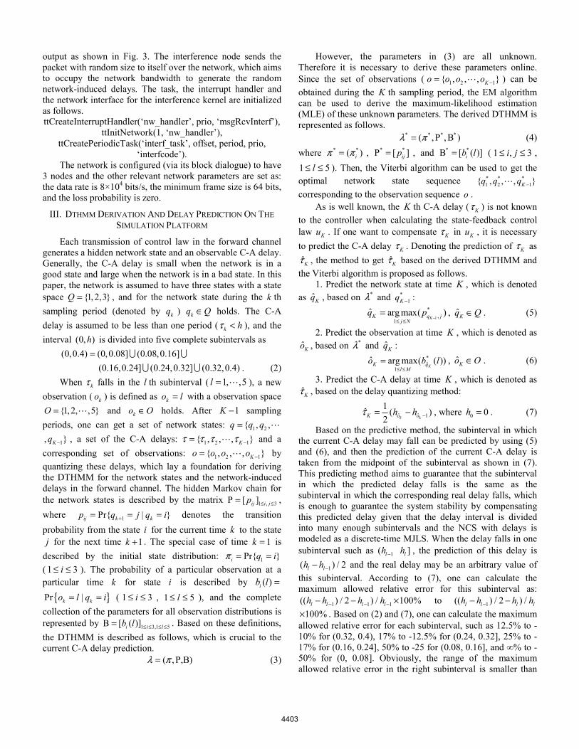
that in the left subinterval. Therefore, when the delay falls in the front part of these subintervals, the predicting method with a relative low accuracy such as in (7) is enough to guarantee that the predicted delay and the real delay fall in the same subinterval. After 500 sampling periods, the real C-A delays are collected in a sequence (τ ) at the controller node as shown in Fig. 4, where the real delays during the first to the 80th sampling period and the 401st to the 500th sampling period fall in the second subinterval (0.08, 0.16], the real delays during the 81st to the 160th sampling period and the 281st to the 400th sampling period fall in the third subinterval (0.16, 0.24], and the real delays during the 161st to the 280th sampling period fall in the fourth subinterval (0.24, 0.32]. During each sampling period, the past real C-A delays are quantized to get the observation sequence ( o ) with the values: 2 for the delays in (0.08, 0.16], 3 for the delays in (0.16, 0.24] and 4 for the delays in (0.24, 0.32]. Based on the quantized sequence, the EM algorithm is used to derive the DTHMM parameters ( * * * *( ,P , B )λ π= ) such as follows based on the past 499 real C-A delays. ( )* 1 0 0π =

*

0.9944 0.0056 0.0000P 0.0050 0.9900 0.0050

0.0000 0.0083 0.9917

⎛ ⎞⎜ ⎟= ⎜ ⎟⎜ ⎟⎝ ⎠

*

0 1 0 0 0B 0 0 1 0 0

0 0 0 1 0

⎛ ⎞⎜ ⎟= ⎜ ⎟⎜ ⎟⎝ ⎠

By using the predictive method in (5)(6)(7), one can get that the prediction of the C-A delay during each sampling period based on the past observation sequence as shown in Fig. 4. During the first to the 80th sampling period, the quantized observation values are all uniquely equal to 2 and the predicted delays are all uniquely equal to 0.12s, which means that the predicted delay and the real delay fall in the same subinterval (0.08, 0.16] with zero absolute error between the predicted observation and the corresponding real observation. However, during the 81st sampling period, the predicted observation value is still 2 while the real C-A delay falls in (0.16, 0.24] with the corresponding real observation value being 3. The reason why there is a non-zero absolute error (actually equal to -1) between the 81st predicted observation and the corresponding real observation is that all the 80 past quantized observation values that are used to train the DTHMM during the 81st sampling period are all equal to 2. Therefore, the predicted observation is still 2 although the real C-A delay falls in (0.16, 0.24] with the real observation value being 3. Similarly, during the 161st sampling period, the predicted observation value is still 3 while the real C-A delay falls in (0.24, 0.32] with the corresponding real observation value being 4, which results in the non-zero absolute error (actually equal to -1) between the 161st predicted observation and the corresponding real observation because that all the 160 past quantized observation values that are used to train the DTHMM during the 161st sampling period only consist of 2 and 3. After the 161st sampling period, the past quantized observation values that are used to train the DTHMM consist

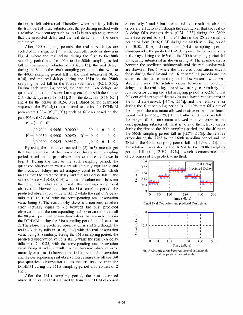
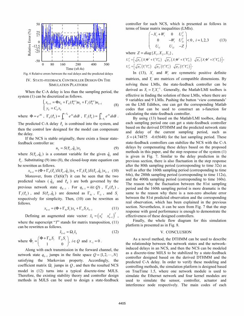
of not only 2 and 3 but also 4, and as a result the absolute errors are all zero even though the subinterval that the real C-A delay falls changes from (0.24, 0.32] during the 280th sampling period to (0.16, 0.24] during the 281st sampling period or from (0.16, 0.24] during the 400th sampling period to (0.08, 0.16] during the 401st sampling period. Consequently, the predicted C-A delays and the corresponding real delays during the 162nd to the 500th sampling period fall in the same subinterval as shown in Fig. 4. The absolute errors between the predicted subintervals and the real subintervals are shown in Fig. 5, where the predicted observations except those during the 81st and the 161st sampling periods are the same as the corresponding real observations with zero absolute errors. The relative errors between the predicted delays and the real delays are shown in Fig. 6. Similarly, the relative error during the 81st sampling period is -32.61% that falls out of the range of the maximum allowed relative error in the third subinterval: [-17%, 25%], and the relative error during the161st sampling period is -16.69% that falls out of the range of the maximum allowed relative error in the fourth subinterval: [-12.5%, 17%]. But all other relative errors fall in the range of the maximum allowed relative error in the corresponding subinterval. That is to say, the relative errors during the first to the 80th sampling period and the 401st to the 500th sampling period fall in [-25%, 50%], the relative errors during the 82nd to the 160th sampling period and the 281st to the 400th sampling period fall in [-17%, 25%], and the relative errors during the 162nd to the 280th sampling period fall in [-12.5%, 17%], which demonstrates the effectiveness of the predictive method.

0 80 160 280 400 5000

0.08

0.16

0.24

0.32

0.4

Time (x0.4s)

Del

ay (s

)

Real DelayPredicted Delay

Fig. 4 Real C-A delays and predicted C-A delays.

0 81 161 300 400 500-1

-0.5

0

Time (x0.4s)

Abs

olut

e Er

ror

Fig. 5 Absolute errors between the real subintervals

and the predicted subintervals

4404

Time (x0.4s)

50

2517

0-12.5

-17-25

-500 80 160 280 400 500

Rel

ativ

e Er

ror (

%)

Fig. 6 Relative errors between the real delays and the predicted delays

IV. STATE-FEEDBACK CONTROLLER DESIGN ON THE SIMULATION PLATFORM

When the C-A delay is less than the sampling period, the system (1) can be discretized as follows.

1 0 1 1ˆ ˆ( ) ( )ca cak k k k k k

k k k

x x u uy C x

τ τ+ −⎧ = Φ + Γ + Γ⎪⎨ =⎪⎩

(8)

where AheΦ = , ˆ

0 0ˆ( ) kh As

k e dsBτ

τ−

Γ = ∫ , 1 ˆˆ( )

k

h Ask h

e dsBτ

τ−

Γ = ∫ .

The predicted C-A delay ˆkτ is combined into the system, and then the control law designed for the model can compensate the delay. If the NCS is stable originally, there exists a linear state-feedback controller as:

ˆ ˆ( , )k k k ku S q xτ= (9) where ˆ ˆ( , )k kS qτ is a constant variable for the given ˆkq and ˆkτ . Substituting (9) into (8), the closed-loop state equation can

be rewritten as follows. 1 0 1 1ˆ ˆ ˆ ˆ ˆ ˆ( ( ) ( , )) ( ) ( , )k k k k k k k k kx S q x S q xτ τ τ τ+ −= Φ + Γ + Γ (10)

Moreover, from (5)(6)(7) it can be seen that the two predicted values ( ˆKq and ˆKτ ) are both governed by the previous network state 1Kq − . For 1 ( )kq i Q− = ∈ , 0 ˆ( )kτΓ ,

1 ˆ( )kτΓ , and ˆ ˆ( , )k kS qτ are denoted as 0iΓ , 1iΓ , and iS respectively for simplicity. Then, (10) can be rewritten as follows.

1 0 1 1( )k i i k i i kx S x S x+ −= Φ + Γ + Γ (11)

Defining an augmented state vector: ( )1

TT Tk k kx x x −= ,

where the superscript “T” stands for matrix transposition, (11) can be rewritten as follows.

1k i kx x+ = Ω (12)

where 0 1

1 0i i i i

i

S SΦ + Γ Γ⎛ ⎞Φ = ⎜ ⎟

⎝ ⎠, i Q∈ and 1 0x− = .

Along with each transmission in the forward channel, the network state 1kq − jumps in the finite space {1,2, , }Q N= satisfying the Markovian property. Accordingly, the coefficient matrix iΩ jumps in Q , and then the resulted NCS model in (12) turns into a typical discrete-time MJLS. Therefore, the existing stability theory and controller design methods in MJLS can be used to design a state-feedback

controller for such NCS, which is presented as follows in terms of linear matrix inequalities (LMIs).

1

2

1 2

00 0

Ti i i

Ti i

i i

X W UW U

U U Z

⎛ ⎞− +⎜ ⎟− <⎜ ⎟⎜ ⎟−⎝ ⎠

, 1, 2,3i = (13)

where 1 2 3{ , , }Z diag X X X= ,

( ) ( ) ( )1 1 0 2 0 3 0T T T T T T T T T Ti i i i i i i i i i i i iU p X Y p X Y p X Y⎡ ⎤= Φ + Γ Φ + Γ Φ + Γ⎣ ⎦

,

( ) ( ) ( )2 1 1 2 1 3 1T T T T T T Ti i i i i i i i i iU p Y p Y p Y⎡ ⎤= Γ Γ Γ⎣ ⎦

.

In (13), iX and iW are symmetric positive definite matrices, and iY are matrices of compatible dimensions. By solving these LMIs, the state-feedback controller can be derived as 1

i i iS Y X −= . Generally, the Matlab/LMI toolbox is effective in finding the solution of these LMIs, where there are 9 variables and 9 LMIs. Pushing the button ‘view commands’ on the LMI Editbox, one can get the corresponding Matlab codes that can be used to construct an s-function for calculating the state-feedback controller. By using (13) based on the Matlab/LMI toolbox, during each sampling period one can get a state-feedback controller based on the derived DTHMM and the predicted network state and delay of the current sampling period, such as

(4.74875 -0.65648)S = for the last sampling period. These state-feedback controllers can stabilize the NCS with the C-A delays by compensating these delays based on the proposed methods in this paper, and the step response of the system (1) is given in Fig. 7. Similar to the delay prediction in the previous section, there is also fluctuation in the step response after the 80th sampling period (corresponding to time 32s) as well as after the 160th sampling period (corresponding to time 64s), the 280th sampling period (corresponding to time 112s), and the 400th sampling period (corresponding to time 160s). The reason why the fluctuation between the 81st sampling period and the 160th sampling period is more dramatic is the same to the reason why there is a non-zero absolute error between the 81st predicted observation and the corresponding real observation, which has been explained in the previous section. Nevertheless, it can be seen from Fig. 7 that the step response with good performance is enough to demonstrate the effectiveness of these designed controllers. Finally, the whole flow diagram for this simulation platform is presented as in Fig. 8.

V. CONCLUSION

As a novel method, the DTHMM can be used to describe the relationship between the network states and the network-induced delays in an NCS, and then the NCS can be modeled as a discrete-time MJLS to be stabilized by a state-feedback controller designed based on the derived DTHMM and the predicted C-A delay. In order to verify these modeling and controlling methods, the simulation platform is designed based on TrueTime 1.5, where one network module is used to simulate the Ethernet network and four kernel modules are used to simulate the sensor, controller, actuator and interference node respectively. The main codes of each

4405

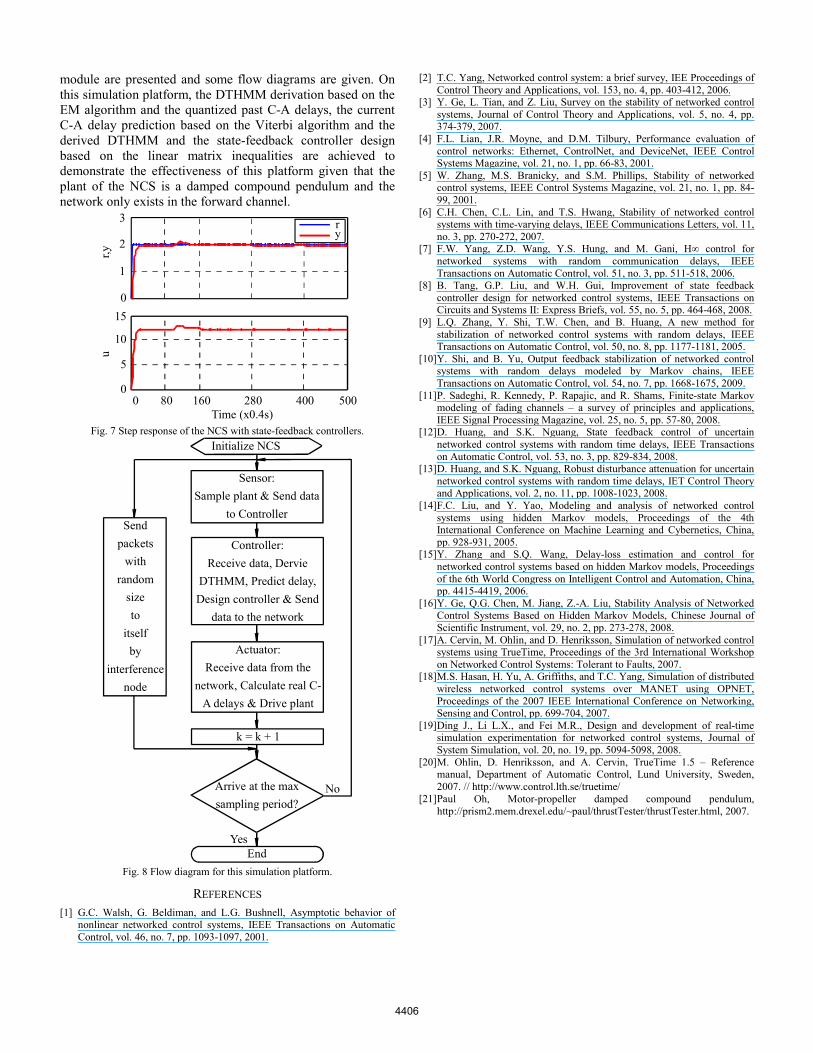
module are presented and some flow diagrams are given. On this simulation platform, the DTHMM derivation based on the EM algorithm and the quantized past C-A delays, the current C-A delay prediction based on the Viterbi algorithm and the derived DTHMM and the state-feedback controller design based on the linear matrix inequalities are achieved to demonstrate the effectiveness of this platform given that the plant of the NCS is a damped compound pendulum and the network only exists in the forward channel.

3

2

1

015

10

5

0

Time (x0.4s)

r,yu

0 80 160 280 400 500

ry

Fig. 7 Step response of the NCS with state-feedback controllers.

Initialize NCS

Sensor:Sample plant & Send data

to Controller

Controller:Receive data, Dervie

DTHMM, Predict delay,Design controller & Send

data to the network

Actuator:Receive data from the

network, Calculate real C-A delays & Drive plant

k = k + 1

Arrive at the maxsampling period?

End

Sendpackets

withrandom

sizeto

itselfby

interferencenode

No

Yes

Fig. 8 Flow diagram for this simulation platform.

REFERENCES [1] G.C. Walsh, G. Beldiman, and L.G. Bushnell, Asymptotic behavior of

nonlinear networked control systems, IEEE Transactions on Automatic Control, vol. 46, no. 7, pp. 1093-1097, 2001.

[2] T.C. Yang, Networked control system: a brief survey, IEE Proceedings of Control Theory and Applications, vol. 153, no. 4, pp. 403-412, 2006.

[3] Y. Ge, L. Tian, and Z. Liu, Survey on the stability of networked control systems, Journal of Control Theory and Applications, vol. 5, no. 4, pp. 374-379, 2007.

[4] F.L. Lian, J.R. Moyne, and D.M. Tilbury, Performance evaluation of control networks: Ethernet, ControlNet, and DeviceNet, IEEE Control Systems Magazine, vol. 21, no. 1, pp. 66-83, 2001.

[5] W. Zhang, M.S. Branicky, and S.M. Phillips, Stability of networked control systems, IEEE Control Systems Magazine, vol. 21, no. 1, pp. 84-99, 2001.

[6] C.H. Chen, C.L. Lin, and T.S. Hwang, Stability of networked control systems with time-varying delays, IEEE Communications Letters, vol. 11, no. 3, pp. 270-272, 2007.

[7] F.W. Yang, Z.D. Wang, Y.S. Hung, and M. Gani, H∞ control for networked systems with random communication delays, IEEE Transactions on Automatic Control, vol. 51, no. 3, pp. 511-518, 2006.

[8] B. Tang, G.P. Liu, and W.H. Gui, Improvement of state feedback controller design for networked control systems, IEEE Transactions on Circuits and Systems II: Express Briefs, vol. 55, no. 5, pp. 464-468, 2008.

[9] L.Q. Zhang, Y. Shi, T.W. Chen, and B. Huang, A new method for stabilization of networked control systems with random delays, IEEE Transactions on Automatic Control, vol. 50, no. 8, pp. 1177-1181, 2005.

[10] Y. Shi, and B. Yu, Output feedback stabilization of networked control systems with random delays modeled by Markov chains, IEEE Transactions on Automatic Control, vol. 54, no. 7, pp. 1668-1675, 2009.

[11] P. Sadeghi, R. Kennedy, P. Rapajic, and R. Shams, Finite-state Markov modeling of fading channels – a survey of principles and applications, IEEE Signal Processing Magazine, vol. 25, no. 5, pp. 57-80, 2008.

[12] D. Huang, and S.K. Nguang, State feedback control of uncertain networked control systems with random time delays, IEEE Transactions on Automatic Control, vol. 53, no. 3, pp. 829-834, 2008.

[13] D. Huang, and S.K. Nguang, Robust disturbance attenuation for uncertain networked control systems with random time delays, IET Control Theory and Applications, vol. 2, no. 11, pp. 1008-1023, 2008.

[14] F.C. Liu, and Y. Yao, Modeling and analysis of networked control systems using hidden Markov models, Proceedings of the 4th International Conference on Machine Learning and Cybernetics, China, pp. 928-931, 2005.

[15] Y. Zhang and S.Q. Wang, Delay-loss estimation and control for networked control systems based on hidden Markov models, Proceedings of the 6th World Congress on Intelligent Control and Automation, China, pp. 4415-4419, 2006.

[16] Y. Ge, Q.G. Chen, M. Jiang, Z.-A. Liu, Stability Analysis of Networked Control Systems Based on Hidden Markov Models, Chinese Journal of Scientific Instrument, vol. 29, no. 2, pp. 273-278, 2008.

[17] A. Cervin, M. Ohlin, and D. Henriksson, Simulation of networked control systems using TrueTime, Proceedings of the 3rd International Workshop on Networked Control Systems: Tolerant to Faults, 2007.

[18] M.S. Hasan, H. Yu, A. Griffiths, and T.C. Yang, Simulation of distributed wireless networked control systems over MANET using OPNET, Proceedings of the 2007 IEEE International Conference on Networking, Sensing and Control, pp. 699-704, 2007.

[19] Ding J., Li L.X., and Fei M.R., Design and development of real-time simulation experimentation for networked control systems, Journal of System Simulation, vol. 20, no. 19, pp. 5094-5098, 2008.

[20] M. Ohlin, D. Henriksson, and A. Cervin, TrueTime 1.5 – Reference manual, Department of Automatic Control, Lund University, Sweden, 2007. // http://www.control.lth.se/truetime/

[21] Paul Oh, Motor-propeller damped compound pendulum, http://prism2.mem.drexel.edu/~paul/thrustTester/thrustTester.html, 2007.

4406