Design of Suspension Towers for Transmission Lines Katrine Engebrethsen Civil and Environmental Engineering Supervisor: Arild Holm Clausen, KT Co-supervisor: Árni Björn Jónasson, ARA Engineering Department of Structural Engineering Submission date: January 2017 Norwegian University of Science and Technology

Welcome message from author
This document is posted to help you gain knowledge. Please leave a comment to let me know what you think about it! Share it to your friends and learn new things together.
Transcript
Design of Suspension Towers forTransmission Lines
Katrine Engebrethsen
Civil and Environmental Engineering
Supervisor: Arild Holm Clausen, KTCo-supervisor: Árni Björn Jónasson, ARA Engineering
Department of Structural Engineering
Submission date: January 2017
Norwegian University of Science and Technology


Department of Structural Engineering Faculty of Engineering Science and Technology NTNU- Norwegian University of Science and Technology
MASTER THESIS 2017
SUBJECT AREA:
Design of Structures
DATE:
22. January 2017
NO. OF PAGES:
20+146+98
TITLE:
Design of Suspension Towers for Transmission Lines Prosjektering av Bæremaster for Kraftlinjer
BY:
Katrine Engebrethsen
RESPONSIBLE TEACHER: Arild Holm Clausen SUPERVISOR(S): Árni Björn Jónasson (ARA Engineering), Janos Toth (ARA Engineering) and Rolv Geir Knutsen (ARA Engineering) CARRIED OUT AT: Department of Structural Engineering (NTNU)
SUMMARY:
This thesis is concerned with the design and analysis of suspension towers for transmission lines. Three different portal tower designs are considered; one steel lattice tower, one steel tubular tower and one less conventional made of tubular elements using glass fibre reinforced polymer. A literature study is conducted on tower design, dynamic response of tower structures and composites used in load-bearing structures. The three alternative designs are modelled in PLS-POLE and PLS-TOWER and the 4.5 km long transmission line is modelled in PLS-CADD where the towers are applied climatic loading and analysed. The towers are then optimised and checked by hand-calculations. A life cycle cost analysis on net present value, including a sensitivity analysis, and an environmental life cycle assessment on CO2-emissions are conducted. The three towers are then compared based on material preference and the analysis results. This results in the two tubular towers being the most economical alternatives, while the two steel towers are the most environmentally friendly.
ACCESSIBILITY
OPEN
i


PrefaceThis master thesis represent the final part of a 5 year M.Sc Degree at theDepartment of Structural Engineering, with a specialisation in Design ofStructures, at the Norwegian University of Science and Technology (NT-NU). The master thesis was initiated in collaboration with ARA Engineer-ing and was carried out over a time period of 21 weeks from September2016 to January 2017. ARA Engineering has provided the relevant soft-ware and design standards for the different parts of the study.
First of all, I would like to thank ARA Engineering for giving me this op-portunity and creating an interesting problem to be addressed, and for hos-ting me in Reykjavik for one month in September 2017. I would especiallylike to thank my supervisors Arni Bjorn Jonasson, Janos Toth and RolvGeir Knutsen for all their advice, guidance and interesting discussions.
I would also like to thank professor Arild Holm Clausen at NTNU for hishelp and guidance.
Furthermore, I would like to thank everybody else at ARA Engineering whohelped me, a special thanks to Thorgeir Holm Olafsson for all his help withthe PLS-modelling and to both Katarzyna Mazur-Pytlowany and ThorgeirHolm Olafsson for advising the PLS-courses I was allowed to attend inSeptember 2017.
Finally, I would like to thank my family for all their help during the pastfew months and all their insightful input.
Trondheim, 22. January 2017
Katrine Engebrethsen
iii

Abstract
This thesis is concerned with the design and analysis of guyed suspensiontowers for transmission lines. The line is thought located somewhere inNorway and the design requirements are therefore based on European andNorwegian standards and national normative aspects.
Three different designs are considered for these 420 kV guyed portal tow-ers. Two are designed using steel; one latticed and one made of tubularelements. The third tower is of a less conventional design made of tubularelements using glass fibre reinforced polymer. All the tower designs are 25m high to the cross arm, with three triplex phases and two ground wires.The three phases are attached to the tower using V-insulator chains with acentre distance of 9 m between the conductors.
A literature study is conducted on tower design, dynamic response of towerstructures and composites and their use in load-carrying structures.
The three alternative designs are modelled in PLS-POLE and PLS-TOWERand the 4.5 km long transmission line is modelled in PLS-CADD wherethe towers are applied climatic loading according to the standards, and ana-lysed. Hand calculations are done to find preliminary cross sections and toverify the loads applied in the program. The cross sections are then optimi-sed in the programs based on the load cases.
The deflections of the towers are then checked and the structures are foundto be adequate. The natural frequencies of conductors and towers are deter-mined for two wind load cases and are found to not coincide, meaning theywill not excite each other. The steel poles are checked against buckling.
A life cycle cost analysis determining the net present value of the threetower designs is conducted, including a sensitivity analysis. In addition, anenvironmental life cycle assessment is conducted to determine the environ-mental impact based emissions of CO2-equivalents. The design using FRPis found to be the most economic, but highest in regard to emissions. Thetwo steel towers score fairly similarly when it comes to emissions, but thelattice design comes out last in regard to net present value.
v
A comparison of the three tower designs is also done based on materialperformance. Both steel and FRP offer good material properties, but theFRP has some advantages because of its non-conductivity and low weightthat increases the safety of workers.
The material costs are found to be 165740 NOK for the steel lattice tower,195500 NOK for the steel tubular tower and 233800 NOK for the FRPtubular tower.
vi
Sammendrag
Denne masteroppgaven tar for seg design og analyse av bardunerte bære-master for kraftlinjer. Linjen er tenkt plassert et sted i Norge og kravene tilutforming er derfor stilt i henhold til europeiske og norske standarder ognasjonale tillegg.
Tre ulike utforminger er vurdert for disse 420 kV bardunerte portalmaste-ne. To er designet ved bruk av stal; en gittermast og en rørmast. Den tredjemasten er ogsa en rørmast, men tar i bruk det mindre konvensjonelle mate-rialet glassfiberforsterket polymer. Alle mastene er 25 m høye til traversen,med tre triplex faser og to toppliner. De tre fasene er opphengt ved bruk avV-isolatorkjeder med en senteravstand pa 9 m mellom fasene.
En litteraturstudie er gjennomført for a se pa masteutforming, dynamiskrespons av master og kompositter og deres anvendelse i lastbærende kon-struksjoner.
De tre alternative utformingene er modellert i PLS-POLE og PLS-TOWERog den 4,5 km lange kraftlinjen er modellert i PLS-CADD hvor maste-ne blir paført klimatisk belasting i henhold til standardene, og analysert.Handberegninger gjøres for a finne foreløpige tverrsnitt og for a kontrollerelastene som paføres i programmene. Tverrsnittene blir deretter optimaliserti programmene basert pa de ulike lasttilfellene.
Utbøyinger av mastene blir sa kontrollert og konstruksjonene er funnet til avære tilstrekkelige. Egenfrekvensene til kablene og mastene er fastsatt forto vindlasttilfeller og er funnet til a ikke sammenfalle. Det skapes altsa ikkeresonans. Stalrørene i beina av rørmasten er kontrollert mot knekking.
En livssykluskostnadsanalyse (LCC) for a bestemme naverdien av de treutformingene er gjennomført, inkludert en sensitivitetsanalyse. I tillegg eren miljølivssyklusanalyse (LCA) utført for a bestemme miljøbelastningenbasert pa utslipp av CO2-ekvivalenter. Utformingen i FRP er funnet til avære den mest økonomiske, men gir størst utslipp. De to stalmastene scorerganske likt nar det gjelder utslipp, men gittermasten kommer darligst utmed tanke pa naverdi.
vii

De tre utformingene blir ogsa sammenlignet pa bakgrunn av materialegen-skaper. Bade stal og FRP tilbyr gode materialegenskaper, men FRP harnoen fordeler grunnet sine isolerende egenskaper og lav vekt som øker sik-kerheten for arbeiderne.
Materialkostnadene er funnet til a være 165740 NOK for gittermasten istal, 195500 NOK for rørmasten i stal og 233800 NOK for rørmasten ikompositt.
viii
Contents
Preface iii
Abstract v
Sammendrag vii
Table of Contents xiv
Nomenclature xv
Abbreviations xvii
1 Introduction 1
2 Literature Review 3
2.1 Transmission lines and structures . . . . . . . . . . . . . . 3
2.2 Dynamic response of tower structures . . . . . . . . . . . 10
2.3 Steel . . . . . . . . . . . . . . . . . . . . . . . . . . . . . 14
ix
2.3.1 Material properties . . . . . . . . . . . . . . . . . 15
2.4 Composite materials . . . . . . . . . . . . . . . . . . . . 15
2.4.1 Fibre Reinforced Polymers . . . . . . . . . . . . . 16
2.4.2 Manufacturing processes of FRPs . . . . . . . . . 18
2.4.3 Properties of Fibre Reinforced Polymers . . . . . . 19
2.5 Application of composites in load-carrying structures . . . 20
3 Design 23
3.1 Basis for Design . . . . . . . . . . . . . . . . . . . . . . . 23
3.2 Limit states . . . . . . . . . . . . . . . . . . . . . . . . . 24
3.3 Line location . . . . . . . . . . . . . . . . . . . . . . . . 25
3.4 Tower structure and geometry . . . . . . . . . . . . . . . 25
3.4.1 Steel lattice tower . . . . . . . . . . . . . . . . . . 30
3.4.2 Steel tubular tower . . . . . . . . . . . . . . . . . 34
3.4.3 FRP tubular tower . . . . . . . . . . . . . . . . . 37
4 Actions on Lines 41
4.1 Dead load . . . . . . . . . . . . . . . . . . . . . . . . . . 42
4.2 Temperature load . . . . . . . . . . . . . . . . . . . . . . 43
4.3 Wind load . . . . . . . . . . . . . . . . . . . . . . . . . . 43
4.4 Ice load . . . . . . . . . . . . . . . . . . . . . . . . . . . 47
4.5 Combined wind and ice load . . . . . . . . . . . . . . . . 49
x
4.6 Security loads . . . . . . . . . . . . . . . . . . . . . . . . 52
4.7 Safety loads . . . . . . . . . . . . . . . . . . . . . . . . . 52
4.8 Other loads . . . . . . . . . . . . . . . . . . . . . . . . . 53
4.9 Load cases . . . . . . . . . . . . . . . . . . . . . . . . . . 54
5 Modelling 59
5.1 Modelling of Line in PLS-CADD . . . . . . . . . . . . . 60
5.1.1 Terrain . . . . . . . . . . . . . . . . . . . . . . . 60
5.1.2 Basis for Criteria . . . . . . . . . . . . . . . . . . 64
5.1.3 Detailed Criteria . . . . . . . . . . . . . . . . . . 66
5.1.4 Basis for Calculating Structure Strength . . . . . . 72
5.1.5 Basis for Calculating Tension and Sag in Cables . 75
5.1.6 Reports . . . . . . . . . . . . . . . . . . . . . . . 84
5.1.7 Structure and Section Modelling . . . . . . . . . . 85
5.2 Modelling in PLS-TOWER . . . . . . . . . . . . . . . . . 86
5.2.1 Basis for Modelling . . . . . . . . . . . . . . . . 86
5.2.2 Steel Lattice Tower Model . . . . . . . . . . . . . 92
5.3 Modelling in PLS-POLE . . . . . . . . . . . . . . . . . . 95
5.3.1 Basis for Modelling . . . . . . . . . . . . . . . . 95
5.3.2 Steel Tubular Tower Model . . . . . . . . . . . . . 99
5.3.3 FRP Tubular Tower Model . . . . . . . . . . . . . 101
xi
6 Calculations and Checks 105
6.1 Preliminary Calculations . . . . . . . . . . . . . . . . . . 105
6.1.1 Vertical loads . . . . . . . . . . . . . . . . . . . . 105
6.1.2 Transverse loads . . . . . . . . . . . . . . . . . . 106
6.1.3 Longitudinal loads . . . . . . . . . . . . . . . . . 107
6.1.4 Combined Forces . . . . . . . . . . . . . . . . . . 107
6.1.5 Cross Sections . . . . . . . . . . . . . . . . . . . 108
6.2 PLS-checks . . . . . . . . . . . . . . . . . . . . . . . . . 109
6.2.1 Load calculation . . . . . . . . . . . . . . . . . . 109
6.2.2 Deflections . . . . . . . . . . . . . . . . . . . . . 109
6.2.3 Dynamic Response . . . . . . . . . . . . . . . . . 110
6.2.4 Buckling of Steel Poles . . . . . . . . . . . . . . . 110
7 Life Cycle Analyses 113
7.1 Theory . . . . . . . . . . . . . . . . . . . . . . . . . . . . 114
7.1.1 Life Cycle Cost . . . . . . . . . . . . . . . . . . . 114
7.1.2 Life Cycle Assessment . . . . . . . . . . . . . . . 115
7.2 Conducted Analyses . . . . . . . . . . . . . . . . . . . . 118
7.2.1 Assumptions . . . . . . . . . . . . . . . . . . . . 118
7.2.2 Life Cycle Cost Analysis . . . . . . . . . . . . . . 121
7.2.3 Life Cycle Assessment . . . . . . . . . . . . . . . 124
xii
8 Discussion 127
8.1 Material Properties . . . . . . . . . . . . . . . . . . . . . 127
8.1.1 Use in Electrical Utility Applications . . . . . . . 128
8.2 Tower Designs . . . . . . . . . . . . . . . . . . . . . . . 131
8.3 LCCA and LCA . . . . . . . . . . . . . . . . . . . . . . . 134
9 Conclusion 139
Bibliography 141
Appendices A1
A Load cases . . . . . . . . . . . . . . . . . . . . . . . . . . A1
B Derivations . . . . . . . . . . . . . . . . . . . . . . . . . B3
B.1 Transverse Forces Derivation . . . . . . . . . . . . B3
B.2 Longitudinal Forces Derivation . . . . . . . . . . B6
C Calculations and Checks . . . . . . . . . . . . . . . . . . C11
C.1 Wind Loads . . . . . . . . . . . . . . . . . . . . . C11
C.2 Ice Loads . . . . . . . . . . . . . . . . . . . . . . C18
C.3 Combined Wind and Ice Loads . . . . . . . . . . . C19
C.4 Ground Wire Tension . . . . . . . . . . . . . . . . C22
C.5 Vertical Loads . . . . . . . . . . . . . . . . . . . C23
C.6 Transverse Loads . . . . . . . . . . . . . . . . . . C30
xiii
C.7 Cross Sections . . . . . . . . . . . . . . . . . . . C32
C.8 Dynamic Response . . . . . . . . . . . . . . . . . C36
C.9 Buckling check of steel poles . . . . . . . . . . . C41
D Input from PLS-programs . . . . . . . . . . . . . . . . . . D57
D.1 Input for Transmission Line from PLS-CADD . . D57
D.2 Input for Steel Lattice Tower from PLS-TOWER . D66
D.3 Input for Steel Tubular Tower from PLS-POLE . . D72
D.4 Input for FRP Tubular Tower from PLS-POLE . . D78
E LCC and LCA . . . . . . . . . . . . . . . . . . . . . . . . E85
E.1 LCC . . . . . . . . . . . . . . . . . . . . . . . . . E85
E.2 LCA . . . . . . . . . . . . . . . . . . . . . . . . E88
E.3 Sensitivity Analysis . . . . . . . . . . . . . . . . E91
xiv
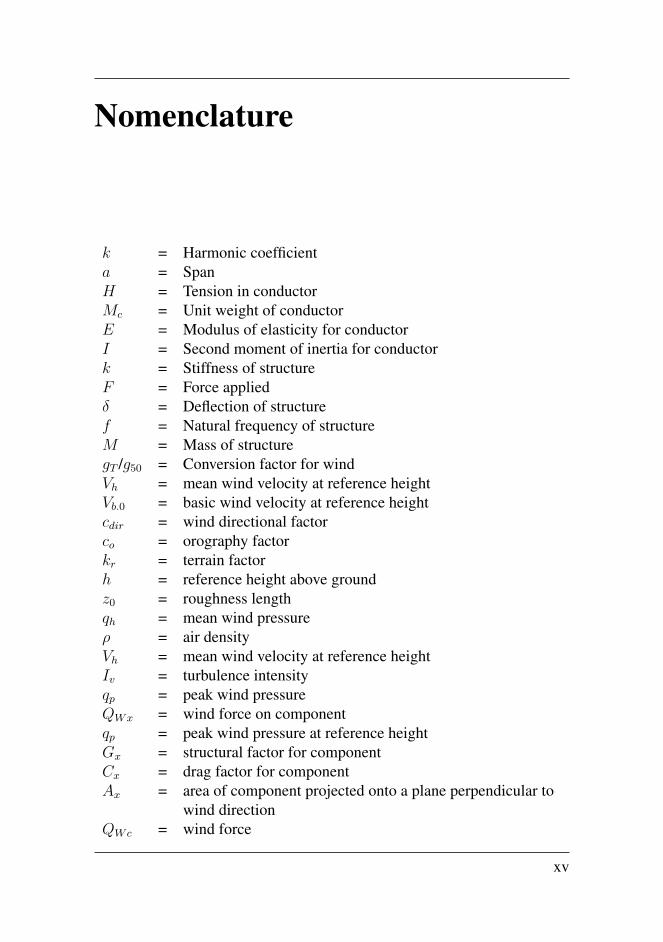
Nomenclature
k = Harmonic coefficienta = SpanH = Tension in conductorMc = Unit weight of conductorE = Modulus of elasticity for conductorI = Second moment of inertia for conductork = Stiffness of structureF = Force appliedδ = Deflection of structuref = Natural frequency of structureM = Mass of structuregT /g50 = Conversion factor for windVh = mean wind velocity at reference heightVb.0 = basic wind velocity at reference heightcdir = wind directional factorco = orography factorkr = terrain factorh = reference height above groundz0 = roughness lengthqh = mean wind pressureρ = air densityVh = mean wind velocity at reference heightIv = turbulence intensityqp = peak wind pressureQWx = wind force on componentqp = peak wind pressure at reference heightGx = structural factor for componentCx = drag factor for componentAx = area of component projected onto a plane perpendicular to
wind directionQWc = wind force
xv

qp = peak wind pressure at reference heightGc = structural factor for conductorCc = drag factor for conductord = diameter of conductorL1 = length of span 1L2 = length of span 2φ = angle between wind direction and the longitudinal axis of
the cross armI = ice load per length of the conductor [N/m]Lw1 = weight span of span 1 of adjacent spansLw2 = weight span of span 2 of adjacent spansI3 = nominal ice load with return period of 3 yearsΨI = combination factor for ice loadI50 = structural factor for conductorVIL = wind velocity of low probabilityVT = wind velocity with given return periodBI = reduction factor for wet snowD = equivalent diameter of ice-covered conductord = diameter of bare conductorI = ice load per lengthρI = ice densityQWIc = wind forceqIp = peak wind pressure at reference heightGc = structural factor for conductorCIc = drag factor for ice-covered conductorD = equivalent diameter of ice-covered conductorL1 = length of span 1L2 = length of span 2φ = angle between wind direction and the longitudinal axis of the
cross-armDel = 2.8m = Required electrical clearancehsnow = 0.5m = Height of snowNPV = net present valueCt = cost in year tr = discount ratet = year
xvi

AbbreviationsFRP = Fibre Reinforced PolymerGFRP = Glass Fibre Reinforced PolymerACSR = Aluminium conductor steel reinforcedACAR = Aluminium conductor alloy reinforcedSSAC = Steel Supported Aluminium ConductorCRS-tower = cross-rope suspension towerV-, M-, Y-, H-tower = tower where legs make the shape of a V, M, Y, HPLS = Power Line SystemsLCC = Life Cycle CostLCCA = Life Cycle Cost AnalysisLCA = Life Cycle AssessmentNPV = Net present value
xvii

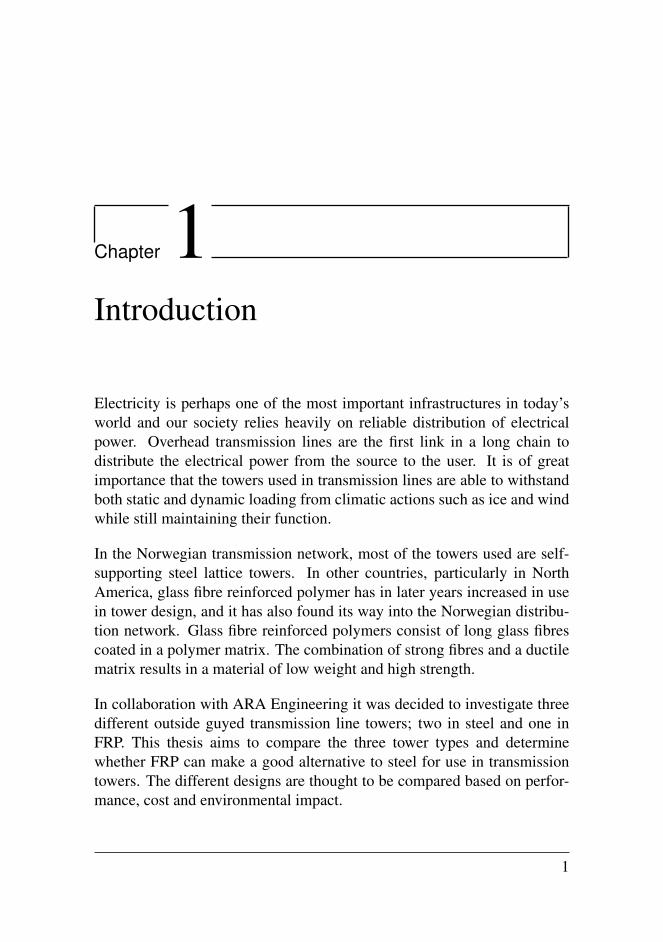
Chapter 1Introduction
Electricity is perhaps one of the most important infrastructures in today’sworld and our society relies heavily on reliable distribution of electricalpower. Overhead transmission lines are the first link in a long chain todistribute the electrical power from the source to the user. It is of greatimportance that the towers used in transmission lines are able to withstandboth static and dynamic loading from climatic actions such as ice and windwhile still maintaining their function.
In the Norwegian transmission network, most of the towers used are self-supporting steel lattice towers. In other countries, particularly in NorthAmerica, glass fibre reinforced polymer has in later years increased in usein tower design, and it has also found its way into the Norwegian distribu-tion network. Glass fibre reinforced polymers consist of long glass fibrescoated in a polymer matrix. The combination of strong fibres and a ductilematrix results in a material of low weight and high strength.
In collaboration with ARA Engineering it was decided to investigate threedifferent outside guyed transmission line towers; two in steel and one inFRP. This thesis aims to compare the three tower types and determinewhether FRP can make a good alternative to steel for use in transmissiontowers. The different designs are thought to be compared based on perfor-mance, cost and environmental impact.
1
Chapter 1. Introduction
A common way to determine the costs of long term investments is by con-ducting a life cycle cost analysis where the present values of all future costsare determined. The environmental impact is similarly determined by anenvironmental life cycle assessment, where the towers’ global warming po-tential is considered based on their emissions of CO2-equivalents.
The transmission line and towers are modelled according to the require-ments and common specifications given in FprEN 50341-1 - Overhead elec-trical lines exceeding AC 1 kV, and the specifications given in the Norwe-gian National Normative Aspects. This is done using software from PowerLine Systems Inc.: PLS-CADD, PLS-POLE and PLS-TOWER.
2
Chapter 2Literature Review
2.1 Transmission lines and structures
The Norwegian electrical power network is divided into three levels. Thetransmission network (main grid) is mostly used for voltages of 420 kV and300 kV, but there are lines with voltages down to 132 kV. The regional dis-tribution network is used for voltages between 36 and 132 kV. And the localdistribution network is used for voltages from 0.23 to 36 kV. In Norway, themain grid is operated by Statnett SF. They are responsible for the operationof about 11000 km of high-voltage power lines (Statnett SF, (2016)). Inmuch of Europe there are only two levels: the transmission network anddistribution network. Much indicates that this will soon be applied in Nor-way as well.
Transmission lines are thus used for transmitting electrical power from gen-erating stations to substations to be distributed further or by interconnectingor adding to existing networks (Kiessling et al., (2003)).
As discussed by Kiessling et al. ((2003)) the use of overhead transmissionlines is a preferred alternative to underground cables, especially for highertransmission voltages. This is much based on an economic aspect as un-derground cables can be 5 to 15 times more expensive than overhead trans-mission lines. Also the fact that maintenance and repair is a lot easier and
3
Chapter 2. Literature Review
less costly can affect this decision. Not all locations are however appropri-ate for overhead transmission lines, such as in near proximity to airports,substation getaways or ocean crossings. Also, when crossing nature con-servation areas underground cables are used more and more. Factors suchas environmental impact are difficult to assess, and while the constructionof a line might be justified, it might still create public reactions (Kiesslinget al., (2003)). Thus, planning is key when considering the construction ofa new line.
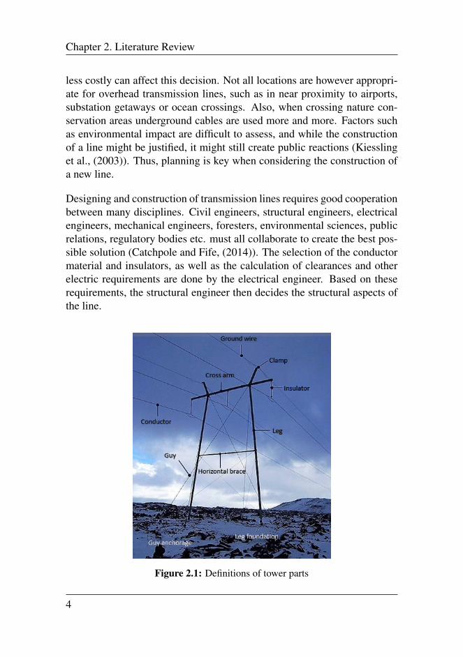
Designing and construction of transmission lines requires good cooperationbetween many disciplines. Civil engineers, structural engineers, electricalengineers, mechanical engineers, foresters, environmental sciences, publicrelations, regulatory bodies etc. must all collaborate to create the best pos-sible solution (Catchpole and Fife, (2014)). The selection of the conductormaterial and insulators, as well as the calculation of clearances and otherelectric requirements are done by the electrical engineer. Based on theserequirements, the structural engineer then decides the structural aspects ofthe line.
Figure 2.1: Definitions of tower parts
4
2.1 Transmission lines and structures
Figure 2.1 illustrates different parts of a transmission line, particularly con-cerning the transmission tower.
In regard to the structural part, the first thing to consider when designinga new line is what type of structures to use. This will depend a lot on theterrain beneath the line and how the structure should help distributing forcesthroughout the line. Kiessling et al. ((2003) divides structures into severalcategories based on their structural purpose.
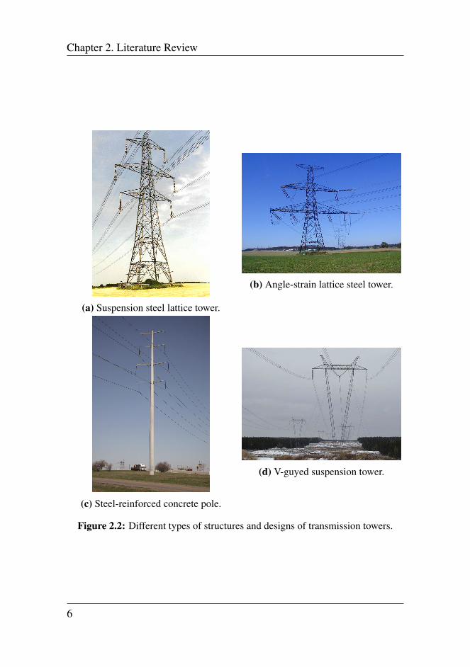
Suspension structures carry the conductor in a straight line and do nottransfer conductor tensile forces. Relatively light-weight and eco-nomic. An example is shown in Figure 2.2a.
Angle suspension structures are used when lines change direction withless than 20 degrees. They do not transfer conductor tensile forces.
Angle structures are used when lines change direction with more than 20degrees. They carry the resulting conductor tensile forces and areequipped with tension insulator sets.
Strain and angle-strain structures carry conductor tensile forces in linedirection or resultant direction respectively. They can withstand dif-fering tensile forces on either side and therefore serve as rigid pointsin the line. To limit cascading they should be arranged regularlyalong the line (every 5-10 km). An example of an angle-strainedstructure is shown in Figure 2.2b.
Dead-end structures carry the total conductor load. They are used wherethe line ends and the conductors are transferred to substation portals.
Special structures are used when a structure has several functions. Forexample, for a T-off structure, where some circuits pass through andothers branch off.
5
Chapter 2. Literature Review
(a) Suspension steel lattice tower.
(b) Angle-strain lattice steel tower.
(c) Steel-reinforced concrete pole.
(d) V-guyed suspension tower.
Figure 2.2: Different types of structures and designs of transmission towers.
6
2.1 Transmission lines and structures
The selection of structure design for an overhead transmission line dependson several parameters. The impact of these will vary from line to line andwill need to be considered for each new line being designed. The followingparameters are given as the most important ones by Kiessling et al. ((2003).
• land used
• environmental impact
• capability to transfer necessary power
• life time
• location and importance
• terrain and access
• number of circuits
• loads
• necessary height
• the use of nearby land
• right-of-way and compensations
• keraunic level and arrangement of ground wires
• construction method and maintenance
• investment
The main categories of structure designs to be considered according toKiessling et al. ((2003) are self-supporting lattice steel towers, self-supportingsteel poles, steel-reinforced concrete poles, wooden poles, guyed structuresand cross-armless structures. A brief description of these follows.
Self-supporting lattice steel towers are the most traditional tower type.They can be used where it is called for narrow towers and can ac-commodate several circuits and all conductor configurations. Theyare easy to transport and relatively economic, also for high towers.Updating and maintenance is easy. They are corrosion protected re-sulting in a long life cycle. The towers require a lower amount ofsteel than similar self-supporting tubular towers. Two examples areshown in Figure 2.2a and Figure 2.2b.
7
Chapter 2. Literature Review
Self-supporting steel poles are used in urban or suburban areas, wherelimited right of way is available. To some they offer a more aestheticoption. These poles can be either suspension poles made of H-beamsections, seamless tubular steel poles with section by section differ-ing diameters or continuously conical shape or conical steel poleswith six, eight or more sides. The suspension poles are generallyof higher cost than lattice towers due to the increased weight. Theseamless tubular poles require expensive equipment for production.Conical sided poles can be adjusted to fit the loads.
Steel-reinforced concrete poles are used in residential areas due to aes-thetics. They require a lower amount of steel, leading to lower coststhan steel towers. Due to the high weight, brittle material and spe-cial equipment needed the transport and erection is more difficult andcostly. They are only available for shorter towers. The concrete sur-face can cause long service life if maintained, but may be reduced byfreeze and thaw and in coastal areas by corrosion due to salt. Spunconcrete poles are used for low- and medium-voltage installations.Vibrated concrete poles are used where spun concrete poles are notavailable. Today no concrete poles are erected in Norway and thosethat exist are old ones. An example is shown in Figure 2.2c.
Wooden poles are common in countries where good quality and large quan-tities of timber can be found. As for example in Norway where theyare much used in the regional and local distribution networks (0.23 -132 kV).
Guyed structures are used for single-circuit lines. Guys are installed tosupport the structure. H-types and portal (M-) types have long beenused. In later years, also V-types and Y-types have been used. Theyare aesthetically and economically favourable and often used in flatterrain. They generally yield lower weight, and by that cost, thanself-supporting towers. An example of a V-guyed tower is shown inFigure 2.2d.
Cross rope structures (CRS) , also called Chainets, use tensioned ropesinstead of a cross arm, thus reducing the amount of steel needed forthe structure. They are commonly used for single-circuit lines andrequire wide site areas.
8

2.1 Transmission lines and structures
Guyed towers are based on the principles that a guy wire and a columnare very effective structural components in regard to tension and compres-sion respectively (White, (1993)). Because of the loads taken by the guys,the amount of steel can be reduced compared to self-supporting towers, re-sulting in lighter towers and a more economical and aesthetically pleasingdesign choice. The guyed towers, however, take up more site area thanself-supporting towers due to the guy anchorages and are therefore onlypreferable where space is not a determinative factor, such as in remote ar-eas (White, (1993)).
Figure 2.3: Guyed M-tower
As mentioned, many different designs for guyed structures are available.White ((1993) divides basic types of guyed structures into guyed singlepoles/masts, guyed rigid frames and guyed and hinged/pinned masted struc-tures. Single masts normally use a pinned connection to the foundation andthe guys are often attached close to each other at the pole. Thus, they relyon the mast and guys being designed so that the lines of action of the dif-ferent loads are close to centric to prevent rotations. They are effective asangle towers and dead end towers. Guyed rigid frames are often designedwith one leg and four guys, and a top structure similar to unsupported rigidframes. Y-towers are examples of this type of guyed structure. Pairs ofguys are normally attached at separated points to ensure torsional stability.
9
Chapter 2. Literature Review
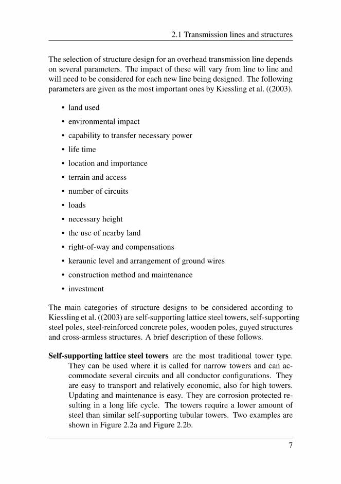
The dimensions of the leg might get quite large to account for moments andshear in the leg if non-centric loads are induced. M-, V- and CRS-towers areexamples of guyed and hinged/pinned masted structures. They often con-sist of two legs and two pairs of guys, attached at each side of a cross armor tensioned wire rope. Due to the guy locations V-towers and CRS-towersare better suited than M-towers if affected by torsional loads. V-towers aremore suitable in uneven terrain since the use of only one footing ensuresequal leg lengths. CRS-towers can be preferred at higher voltages as largeclearance is required and the towers easily can become top heavy. M-towerstake up less space in regard to area than V-towers and CRS-towers, due tothe use of only two guy attachment points. However, higher towers needfour points as the guys need to be crossed to take up the loads, and thus thisadvantage is sometimes lost. An M-tower is illustrated in Figure 2.3. Theconceptual design of these guyed towers are illustrated in Figure 2.4.
Figure 2.4: Conceptual design of guyed towers.
2.2 Dynamic response of tower structures
Structures are often affected by dynamic loads. Dynamic loads are loadsthat are time dependent, whether it be that they only last a small period oftime or that they change greatly with time. A commonly known load suchas this is wind load, which is applied to almost every structure unless builtindoors. For transmission lines wind loading is very common and oftengoverning in design (Gani and Legeron, (2010)). Other dynamic loads canbe earthquake forces and loads from machinery and people.
The dynamic loads that affect structures can excite their natural frequencyif they are of similar size. This can result in either fatigue problems or
10
2.2 Dynamic response of tower structures
structural failure (Vinson and Sierakowski, (2012)). Much theory is avail-able on vibration analysis, which is based on calculus and applied physics(Blevins, (2016)). Names like Euler, Bernoulli, Rayleigh and Timoshenkohave all contributed to the development of the methods used today by in-cluding more parameters.
”The natural frequency of an object is the frequency at which the objectstends to vibrate when disturbed” (The Physics Classroom ((1996-2016)).Adjacent structural parts with similar natural frequencies can excite eachother. Meaning that the conductors excited by the wind can in turn ex-cite the tower structure if the natural frequencies are similar. The resultingresonances can lead to failure (Vinson and Sierakowski, (2012)).
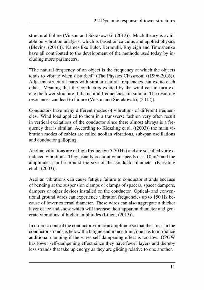
Conductors have many different modes of vibrations of different frequen-cies. Wind load applied to them in a transverse fashion very often resultin vertical excitations of the conductor since there almost always is a fre-quency that is similar. According to Kiessling et al. ((2003)) the main vi-bration modes of cables are called aeolian vibrations, subspan oscillationsand conductor galloping.
Aeolian vibrations are of high frequency (5-50 Hz) and are so called vortex-induced vibrations. They usually occur at wind speeds of 5-10 m/s and theamplitudes can be around the size of the conductor diameter (Kiesslinget al., (2003)).
Aeolian vibrations can cause fatigue failure to conductor strands becauseof bending at the suspension clamps or clamps of spacers, spacer dampers,dampers or other devices installed on the conductor. Optical- and conven-tional ground wires can experience vibration frequencies up to 150 Hz be-cause of lower external diameter. These wires can also aggregate a thickerlayer of ice and snow which will increase their apparent diameter and gen-erate vibrations of higher amplitudes (Lilien, (2013)).
In order to control the conductor vibration amplitude so that the stress in theconductor strands is below the fatigue endurance limit, one has to introduceadditional damping if the wires self-dampening effect is too low. OPGWhas lower self-dampening effect since they have fewer layers and therebyless strands that take up energy as they are gliding relative to one another.
11

Chapter 2. Literature Review
Figure 2.5: Standing waves of 1, 2 and 3 loops (Preformed Line Products, (2016)).
Where bundle conductors are arranged after one another in the directionof the wind subspan oscillations might occur. They are flow-induced vibra-tions and of low frequency, appearing at wind speeds of 4-18 m/s. Differentwind speeds can yield different oscillation modes (Kiessling et al., (2003)).
Conductor galloping usually occurs at wind speeds of 6-25 m/s in bothsingle or bundle conductors. These vibrations are common when wind isapplied to ice covered conductors as the asymmetry of the cables leads toan aerodynamically unstable profile. The transverse force from the windexcites the oscillations further. The amplitude can be as large as the sag ofthe conductor, which can result in clashing and flash overs (Kiessling et al.,(2003)). Galloping can occur as single, double and triple standing wavesas illustrated in Figure 2.5 (Preformed Line Products, (2016)). It is thus forthese number of loops the frequencies of the cables should be assessed.
If the natural frequencies of the towers and conductors coincide, the fre-quency must be altered to avoid negative effects. This can be done in manyways, as discussed by Preformed Line Products ((2016)). Possibly the mostcommon one is to add dampers to the conductors. Others include air flowspoilers and detuning pendulums. Altering the cable span will also have animpact, but might not be the best solution.
The natural frequency of a conductor can be found using Equation 2.2 or2.1 depending on whether the bending stiffness of the conductor should be
12
2.2 Dynamic response of tower structures
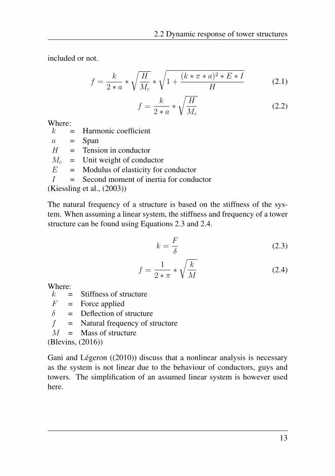
included or not.
f =k
2 ∗ a∗√
H
Mc
∗√
1 +(k ∗ π ∗ a)2 ∗ E ∗ I
H(2.1)
f =k
2 ∗ a∗√
H
Mc
(2.2)
Where:k = Harmonic coefficienta = SpanH = Tension in conductorMc = Unit weight of conductorE = Modulus of elasticity for conductorI = Second moment of inertia for conductor
(Kiessling et al., (2003))
The natural frequency of a structure is based on the stiffness of the sys-tem. When assuming a linear system, the stiffness and frequency of a towerstructure can be found using Equations 2.3 and 2.4.
k =F
δ(2.3)
f =1
2 ∗ π∗√
k
M(2.4)
Where:k = Stiffness of structureF = Force appliedδ = Deflection of structuref = Natural frequency of structureM = Mass of structure
(Blevins, (2016))
Gani and Legeron ((2010)) discuss that a nonlinear analysis is necessaryas the system is not linear due to the behaviour of conductors, guys andtowers. The simplification of an assumed linear system is however usedhere.
13
Chapter 2. Literature Review
2.3 Steel
Steel has been used as a material for many years, both as a building mate-rial and for other uses. Its high strength and ductility, as well as its goodformability and weldability makes it a preferred material in many settings.In later years, the development of the material has allowed it to become oneof the most used construction materials.
Steel is an alloy based on iron with up to 2.1% carbon. Structural steel how-ever, has a considerably lower amount of carbon and is also added severalother alloying elements. These elements greatly affect the material proper-ties of the steel. Structural steel can be divided into normal structural steel,stainless steel and cast steel, but is better classified by its strength class andby its quality. The strength class specifies the steel’s yield stress while thequality specifies the chemical composition, thermal and mechanical pro-cessing and the impact strength of the steel (Larsen, (2015)).
The manufacturing process for steel has stayed more or less the same for100 years. This process can be divided into five steps; reduction, oxidation,deoxidation, casting and rolling.
In the reduction step, pellets from the iron ore, coke and lime stone areadded to the top of a blast furnace, where heated air is applied through thebottom. This turns it into pig iron and slag. The pig iron has a carbon con-centration of 3-5% and contains unwanted elements, such as phosphorusand sulphur.
In the oxidation step the carbon concentration is lowered by adding oxygenso that CO2 is produced. This increases the concentration of oxygen whichcan create pores in the material. This is called rimmed steel.
To reduce the pore formation, alloying elements that react with oxygen areadded in the deoxidation step. Especially ferrosilicon and ferromanganeseare used for this process. Depending on the amount of deoxidation doneone can be left with killed or half-killed steel, where killed steel has beencompletely deoxidized.
The steel will now have the desired properties and is transferred to rolling
14
2.4 Composite materials
mills for further processing. An alternative to this last step is to producecasting blocks that are cooled and then sent to the rolling mills where it canbe reheated and processed further (Larsen, (2015)). For use in electricalutility fully killed steel should be used for angles and plates to ensure thematerial can withstand not only the static loading, but also alternating loadsand possible vibrations (Kiessling et al., (2003)).
2.3.1 Material properties
The material properties of the steel are determined by the amount of differ-ent elements in the steel. These elements include aluminium, phosphorus,hydrogen, copper, chromium, manganese, nickel, nitrogen, oxygen, siliconand sulphur. The effect of these elements is discussed by many, for ex-ample by Larsen ((2015)). As the chemical composition of the steel is soimportant to determine the properties, it is regulated by international rulesand regulations. In addition to this, the micro structure of the steel has abig impact on the mechanical properties. The micro structure is a functionof the carbon content and temperature.
2.4 Composite materials
A composite material can be defined as ”a combination of two or morecomponents differing in form or composition on a macro scale, with two ormore distinct phases having recognisable interfaces between them” (Ako-vali et al. ((2001)), pg. 3). This process of combining materials is done toachieve new or improved properties; mainly in regard to physical, mechan-ical or chemical properties (Vinson and Sierakowski, (1993)). Opinions onthe definition differ, especially on whether it should include the level ofscaling.
The art of combining materials to achieve a new material with better prop-erties has been around for many years. It has been used to develop strongermaterials, more ductile materials or just to provide a smoother finish on sur-faces. A much used and well known composite in the construction industry
15
Chapter 2. Literature Review
today is steel reinforced concrete that combines the high tensile strengthof the steel with the compressive strength and lighter weight of concrete(Vinson and Sierakowski, (2012)). The use of composites today can befound everywhere from households to aerospace (Vinson and Sierakowski,(1993)). Some uses are discussed by Sinha and Vinay ((2010)).
Composites usually consist of a reinforcing material incorporated in a ma-trix. The matrix, which is generally of low modulus, is strengthened by theconsiderably stronger and stiffer reinforcement. On a basic level compos-ites can be divided into three structural levels: elemental, micro-structuraland macrostructural. Depending on the properties needed (e.g. applica-tion temperature or conductivity), different matrices can be used. The mostcommon ones are of metal, ceramics, polymer, carbon or a hybrid of these(Vinson and Sierakowski, (2012)). The composite system acts differentlyaccording to how much and what kind of reinforcement is added. In parti-cle strengthened composites, the reinforcing particles only prevent disloca-tions in the matrix while the matrix itself bears the load. In fibre reinforcedcomposites, the reinforcing fibres bear the load while the matrix acts as aload distributor. Laminar composites are another group, where sheets ofreinforcing agents are bonded together. To get the mechanical propertiesneeded one of the most important features concerning composites is theadhesion between fibres and matrix (Akovali et al., (2001)).
2.4.1 Fibre Reinforced Polymers
In the last decade, the use of polymer matrix composites as an engineeringmaterial has become common. When produced using reinforcing fibres theelements can sport good mechanical properties, such as high strength andstiffness, low weight, non-conductivity, high durability and corrosion resis-tance. In addition fibre reinforced polymers can easily be shaped accordingto will (Sinha and Vinay, (2010)).
The fibres can be either continuous or discontinuous and are usually madeof carbon/graphite, glass or aramid. Other fibres used include boron fibres,ceramic fibres and metallic fibres (Akovali et al., (2001)). Carbon fibres areproduced by burning a precursor fibre at high temperatures such that only
16
2.4 Composite materials
the carbon is left. By increasing the temperature graphite fibres are pro-duced (Sinha and Vinay, (2010)). These fibres based on carbon are strongand light, but also very expensive. Due to this composites based on car-bon fibres are often used in aerospace applications (Akovali et al., (2001)).Aramid fibres are produced by spinning a basic polymer into a fibre. Thesefibres are strong, flexible and can be produced into textile, but they are alsoquite expensive and UV-degradable. A known use for aramid fibres arein Kevlar vests. Depending on the manufacturing process used the fibrescan come in different forms. These include woven mats and fabric, rov-ings, yarns and chopped strands (Sinha and Vinay, (2010)). Due to the highcost and electrical conductivity neither carbon fibres or other metallic fibresare used for electrical utility applications. As glass fibres are cheaper andstill offer good material properties these are preferred for electrical utilityapplications.
The matrix comprises of about 30-40 % of the composite and its main func-tion is to serve as a bond between reinforcing components while distribut-ing loads, providing shear, compressive and transverse strength and protect-ing the reinforcement agents from wear (Akovali et al., (2001)). It is usuallyeither consisting of thermoplastic or thermoset resins. The thermoplasticresin is the least used in the composite industry today. During the pro-cessing of thermoplastics, no chemical reaction occurs and only heat andpressure is required to form the parts. It can be reheated and reshaped, andis therefore often used in for example plastic bottles. The thermoset resin,on the other hand, sets permanently after curing as the polymer chains be-come crosslinked resulting in a final rigid matrix (Vinson and Sierakowski,(2012)). In the production of thermosets, a curing agent (catalyst) will beadded and the resin will be applied to a reinforcing material. Due to heatand pressure a chemical reaction will then harden the resin and the partswill be shaped using the desired manufacturing method (Sinha and Vinay,(2010)). The most common thermosets are unsaturated polyesters, epox-ies and polyimides (Akovali et al., (2001)). A more extensive research onthe polymers used in FRPs can be found in Sinha and Vinay ((2010)). Toget the desired properties, colour and filler can be added to the matrix, andsometimes a solvent is also added.
17
Chapter 2. Literature Review
2.4.2 Manufacturing processes of FRPs
The two most used manufacturing processes to make electrical utility ap-plications of FRP are filament winding and pultrusion. In addition to these,several open mould processes (wet lay-up, bag moulding and curing andautoclave moulding) and closed mould processes (transfer moulding, com-pression moulding and injection moulding) are available for manufacturingFRP elements for other uses (Akovali et al., (2001)). Laminar elements arealso possible to create by bonding fibre layers together using a matrix asglue (Vinson and Sierakowski, (2012)).
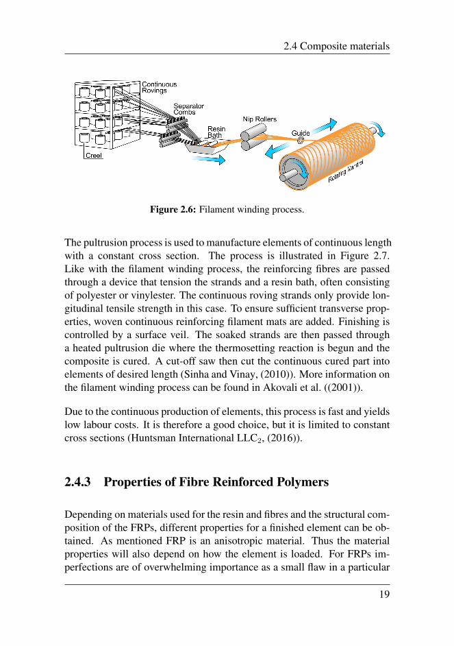
The filament winding process can be done with either wet or pre-impregnatedfibres. The process is illustrated in Figure 2.6. In the wet winding process,which is the most common one, continuous fibre reinforcement, on rovingsis passed through a resin bath. A shuttle will then spin the resin soakedfibres onto a rotating mandrel in a pattern to ensure an even distribution.The angle with which the fibres are spun onto the mandrel is calculated be-forehand for optimum usage according to the external loads. This methodof spinning ensures the element has strength in several directions. Theprocess is done until the desired thickness is achieved. Finally, the spunelement is cured in an oven. It is possible to shape the spun elements intonon-circular shapes before curing. Due to limitations of the size of the ma-chine and oven, only elements up to a certain length can be produced bythis method. The structural elements manufactured in this way are usuallyconical. To get longer elements these can later be stacked. The filamentwinding process is also possible to do using pre-impregnated fibre tows(Sinha and Vinay, (2010)). Over the years, the filament winding processhas become highly automated. This and the progress in analysis programshas made the process from calculations to product both shorter and easier(Peters, (2011)). More information on the filament winding process can befound in Peters ((2011)) and Akovali et al. ((2001)).
Positive aspects with this production method is the automatic process andthat both resin and fibre is used in its lowest cost form. Also, the processresults in members with high mechanical performance. However, costs arehigh due to the investment needed for machines and equipment needed. Inaddition to this, the production series is limited and the use is limited toconvex shaped structures (Huntsman International LLC1, (2013)).
18
2.4 Composite materials
Figure 2.6: Filament winding process.
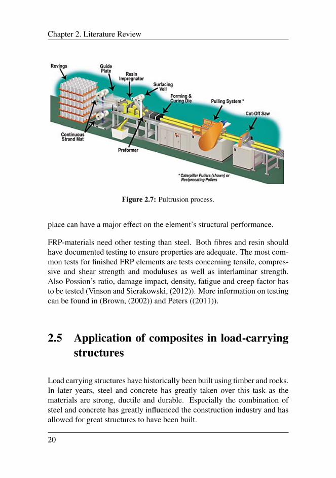
The pultrusion process is used to manufacture elements of continuous lengthwith a constant cross section. The process is illustrated in Figure 2.7.Like with the filament winding process, the reinforcing fibres are passedthrough a device that tension the strands and a resin bath, often consistingof polyester or vinylester. The continuous roving strands only provide lon-gitudinal tensile strength in this case. To ensure sufficient transverse prop-erties, woven continuous reinforcing filament mats are added. Finishing iscontrolled by a surface veil. The soaked strands are then passed througha heated pultrusion die where the thermosetting reaction is begun and thecomposite is cured. A cut-off saw then cut the continuous cured part intoelements of desired length (Sinha and Vinay, (2010)). More information onthe filament winding process can be found in Akovali et al. ((2001)).
Due to the continuous production of elements, this process is fast and yieldslow labour costs. It is therefore a good choice, but it is limited to constantcross sections (Huntsman International LLC2, (2016)).
2.4.3 Properties of Fibre Reinforced Polymers
Depending on materials used for the resin and fibres and the structural com-position of the FRPs, different properties for a finished element can be ob-tained. As mentioned FRP is an anisotropic material. Thus the materialproperties will also depend on how the element is loaded. For FRPs im-perfections are of overwhelming importance as a small flaw in a particular
19
Chapter 2. Literature Review
Figure 2.7: Pultrusion process.
place can have a major effect on the element’s structural performance.
FRP-materials need other testing than steel. Both fibres and resin shouldhave documented testing to ensure properties are adequate. The most com-mon tests for finished FRP elements are tests concerning tensile, compres-sive and shear strength and moduluses as well as interlaminar strength.Also Possion’s ratio, damage impact, density, fatigue and creep factor hasto be tested (Vinson and Sierakowski, (2012)). More information on testingcan be found in (Brown, (2002)) and Peters ((2011)).
2.5 Application of composites in load-carryingstructures
Load carrying structures have historically been built using timber and rocks.In later years, steel and concrete has greatly taken over this task as thematerials are strong, ductile and durable. Especially the combination ofsteel and concrete has greatly influenced the construction industry and hasallowed for great structures to have been built.
20
2.5 Application of composites in load-carrying structures
The use of FRP in structures has mostly been limited to small componentsof buildings, such as window and door details. However, the use has ex-panded to include larger components like roofs, and cladding. Particularlywhen constructing curved roofs or other special structures FRPs can beused to great success. Some expect FRPs to revolutionise the constructionindustry by offering suitable and cost efficient alternatives to traditionalstructures (Kendall, unknown)).
Load carrying parts of structures are important not only for carrying load,but also to ensure the whole structure performs its task in a safe and reliableway. Most of a structure’s weight is often represented by the load carryingpart. FRPs are therefore a good option to use in these parts as they offera high strength to weight ratio. They can also withstand large deflectionswhich can open doors that have previously been closed in regard to materialuse.
FRP offers many advantages for use in load-carrying structures. The lowweight can lead to less heavy lifts and use less heavy equipment, resultingin saved time and cost, which are critical factors in any project. They arevery durable and easy to repair and strengthen in-situ (Halliwell, (2002)).Another major advantage is the possibility to tailor-make the material andits properties to best suit a project, whether it be shape, reinforcement di-rection or colour. The anisotropic nature of FRP, allows for the reinforce-ment to be adjusted to follow stress patterns and lead to economic designs(Kendall, unknown)).
Recently, particularly in North America, FRP has been successfully usedin transmission towers. Another advantage to FRP that directly affects thissection is its insulating properties. By being non-conductive it leads to saferinstallation and maintenance of the transmission lines. Also here, the verygood durability is a great factor.
21

Chapter 3Design
3.1 Basis for Design
Standards:
FprEN 50341-1:2012 E: Overhead electrical lines exceeding AC 1 kV - Part1: General requirements - Common specifications (CENELEC, (2012)) de-fine the basic requirements for design of overhead power lines. It givesrequirements for the reliability, security and safety of the structure.
NO NNA based on EN 50341-3-16:2008 and EN 50423-3-16:2008: Na-tional Normative Aspects for Norway (The Norwegian National Commit-tee, (2008)) defines factors and the like for use in Norway.
NS-EN 1993-1-1:2005+NA:2008: Prosjektering av stalkonstruksjoner - Del1-1: Allmenne regler og regler for bygninger (CEN, (2005)) is the basis forsteel calculations.
Computer programs:
PLS-CADD (Power Line Systems - Computer Aided Design and Drafting)is a design program for overhead power lines from Power Line SystemsInc. It combines terrain modelling, engineering, tower spotting and drafting
23
Chapter 3. Design
(Power Line Systems Inc1, (Updated 2016)). This is used to do the towerspotting of the line.
PLS-TOWER is a program from Power Line Systems Inc for analysingand designing steel latticed towers used in power lines and communicationfacilities. It can perform design checks of the structure under specifiedload cases and calculate wind and weight spans (Power Line SystemsI nc2,(Updated 2016)). PLS-TOWER is used to model the lattice tower.
PLS-POLE is a program from Power Line Systems Inc for analysing anddesigning structures made up of wood, laminated wood, steel, concrete andFibre Reinforced Polymer (FRP) poles or modular aluminium masts. LikeTower it can perform design checks of the structure under specified loadcases and calculate wind and weight spans (Power Line Systems Inc3, (Up-dated 2016)). PLS-POLE is used to model the two towers with tubular legs.
3.2 Limit states
All structures should be checked in the ultimate limit state and the ser-viceability limit state. These limit states are the states where the designrequirements of the overhead line no longer are met (CENELEC, (2012)).
The ultimate limit state is concerned with the structural failure or collapseof a structure due to deformation, stability loss, buckling and so on (CEN-ELEC, (2012)). In the ultimate limit state the structure’s capacity is con-trolled by using the material’s strength parameters and tensile properties todetermine the various elements’ strength and stability due to loading con-ditions based on requirements for safety and reliability (Larsen, (2015)).
In the serviceability limit state, it is checked whether the construction meetsthe requirements set for its purpose and use over its lifetime (Larsen, (2015)).Examples of aspects to check are vibrations, deformations that do not leadto collapse, electrical flashovers and durability (CENELEC, (2012)).
24
3.3 Line location
3.3 Line location
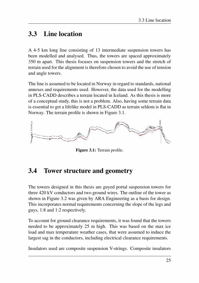
A 4-5 km long line consisting of 13 intermediate suspension towers hasbeen modelled and analysed. Thus, the towers are spaced approximately350 m apart. This thesis focuses on suspension towers and the stretch ofterrain used for the alignment is therefore chosen to avoid the use of tensionand angle towers.
The line is assumed to be located in Norway in regard to standards, nationalannexes and requirements used. However, the data used for the modellingin PLS-CADD describes a terrain located in Iceland. As this thesis is moreof a conceptual study, this is not a problem. Also, having some terrain datais essential to get a lifelike model in PLS-CADD as terrain seldom is flat inNorway. The terrain profile is shown in Figure 3.1.
Figure 3.1: Terrain profile.
3.4 Tower structure and geometry
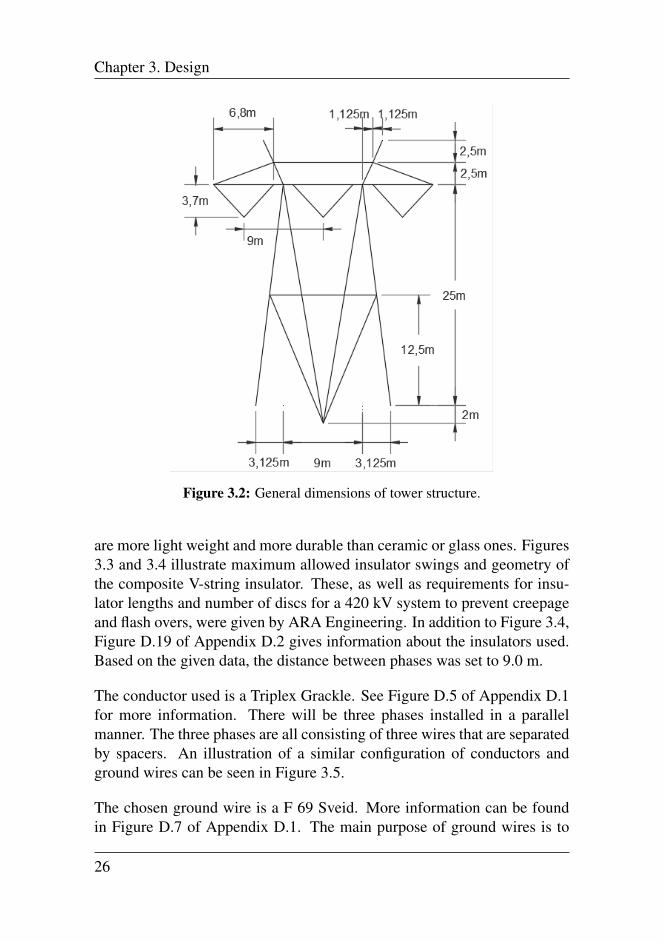
The towers designed in this thesis are guyed portal suspension towers forthree 420 kV conductors and two ground wires. The outline of the tower asshown in Figure 3.2 was given by ARA Engineering as a basis for design.This incorporates normal requirements concerning the slope of the legs andguys, 1:8 and 1:2 respectively.
To account for ground clearance requirements, it was found that the towersneeded to be approximately 25 m high. This was based on the max iceload and max temperature weather cases, that were assumed to induce thelargest sag in the conductors, including electrical clearance requirements.
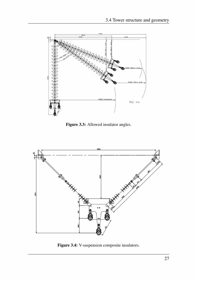
Insulators used are composite suspension V-strings. Composite insulators
25
Chapter 3. Design
Figure 3.2: General dimensions of tower structure.
are more light weight and more durable than ceramic or glass ones. Figures3.3 and 3.4 illustrate maximum allowed insulator swings and geometry ofthe composite V-string insulator. These, as well as requirements for insu-lator lengths and number of discs for a 420 kV system to prevent creepageand flash overs, were given by ARA Engineering. In addition to Figure 3.4,Figure D.19 of Appendix D.2 gives information about the insulators used.Based on the given data, the distance between phases was set to 9.0 m.
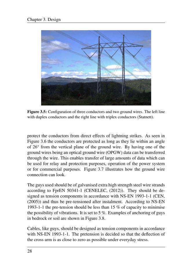
The conductor used is a Triplex Grackle. See Figure D.5 of Appendix D.1for more information. There will be three phases installed in a parallelmanner. The three phases are all consisting of three wires that are separatedby spacers. An illustration of a similar configuration of conductors andground wires can be seen in Figure 3.5.
The chosen ground wire is a F 69 Sveid. More information can be foundin Figure D.7 of Appendix D.1. The main purpose of ground wires is to
26
3.4 Tower structure and geometry
Figure 3.3: Allowed insulator angles.
Figure 3.4: V-suspension composite insulators.
27
Chapter 3. Design
Figure 3.5: Configuration of three conductors and two ground wires. The left linewith duplex conductors and the right line with triplex conductors (Statnett).
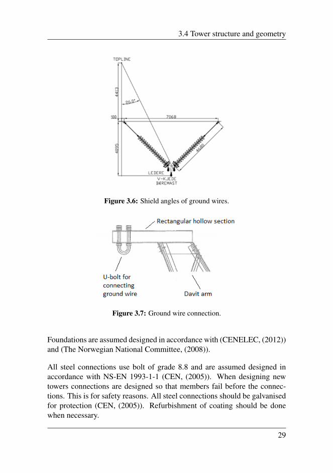
protect the conductors from direct effects of lightning strikes. As seen inFigure 3.6 the conductors are protected as long as they lie within an angleof 26° from the vertical plane of the ground wire. By having one of theground wires being an optical ground wire (OPGW) data can be transferredthrough the wire. This enables transfer of large amounts of data which canbe used for relay and protection purposes, operation of the power systemor for commercial purposes. Figure 3.7 illustrates how the ground wireconnection can look.
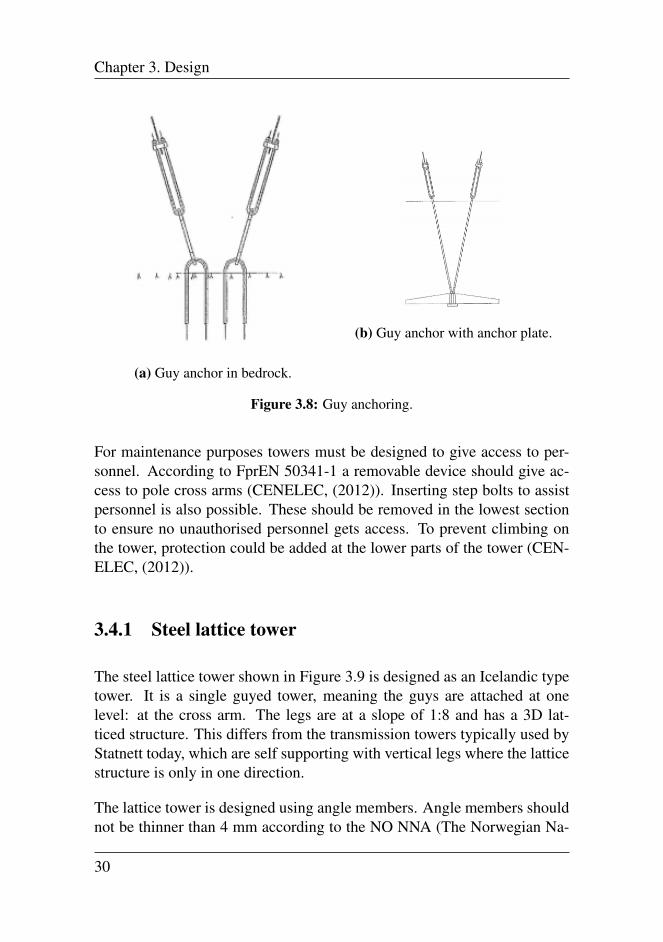
The guys used should be of galvanised extra high strength steel wire strandsaccording to FprEN 50341-1 (CENELEC, (2012)). They should be de-signed as tension components in accordance with NS-EN 1993-1-1 (CEN,(2005)) and thus be pre-tensioned after instalment. According to NS-EN1993-1-1 the pre-tension should be less than 15 % of capacity to minimisethe possibility of vibrations. It is set to 5 %. Examples of anchoring of guysin bedrock or soil are shown in Figure 3.8.
Cables, like guys, should be designed as tension components in accordancewith NS-EN 1993-1-1. The pretension is decided so that the deflection ofthe cross arm is as close to zero as possible under everyday stress.
28
3.4 Tower structure and geometry
Figure 3.6: Shield angles of ground wires.
Figure 3.7: Ground wire connection.
Foundations are assumed designed in accordance with (CENELEC, (2012))and (The Norwegian National Committee, (2008)).
All steel connections use bolt of grade 8.8 and are assumed designed inaccordance with NS-EN 1993-1-1 (CEN, (2005)). When designing newtowers connections are designed so that members fail before the connec-tions. This is for safety reasons. All steel connections should be galvanisedfor protection (CEN, (2005)). Refurbishment of coating should be donewhen necessary.
29
Chapter 3. Design
(a) Guy anchor in bedrock.
(b) Guy anchor with anchor plate.
Figure 3.8: Guy anchoring.
For maintenance purposes towers must be designed to give access to per-sonnel. According to FprEN 50341-1 a removable device should give ac-cess to pole cross arms (CENELEC, (2012)). Inserting step bolts to assistpersonnel is also possible. These should be removed in the lowest sectionto ensure no unauthorised personnel gets access. To prevent climbing onthe tower, protection could be added at the lower parts of the tower (CEN-ELEC, (2012)).
3.4.1 Steel lattice tower
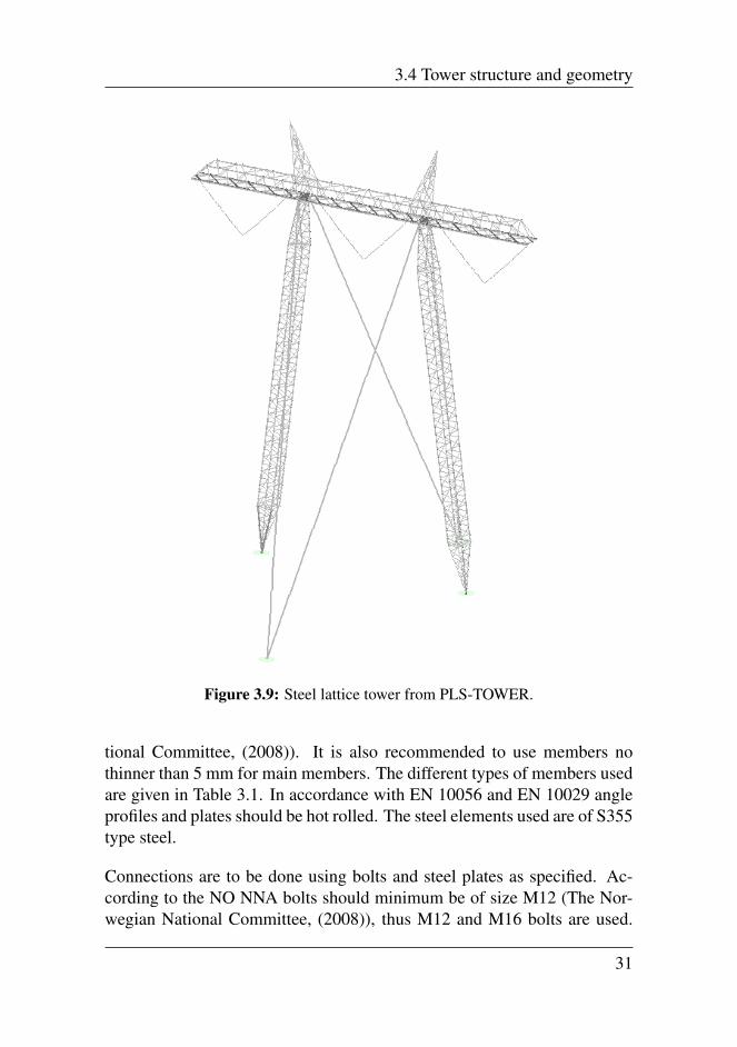
The steel lattice tower shown in Figure 3.9 is designed as an Icelandic typetower. It is a single guyed tower, meaning the guys are attached at onelevel: at the cross arm. The legs are at a slope of 1:8 and has a 3D lat-ticed structure. This differs from the transmission towers typically used byStatnett today, which are self supporting with vertical legs where the latticestructure is only in one direction.
The lattice tower is designed using angle members. Angle members shouldnot be thinner than 4 mm according to the NO NNA (The Norwegian Na-
30
3.4 Tower structure and geometry
Figure 3.9: Steel lattice tower from PLS-TOWER.
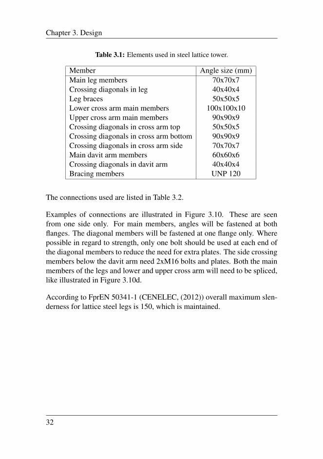
tional Committee, (2008)). It is also recommended to use members nothinner than 5 mm for main members. The different types of members usedare given in Table 3.1. In accordance with EN 10056 and EN 10029 angleprofiles and plates should be hot rolled. The steel elements used are of S355type steel.
Connections are to be done using bolts and steel plates as specified. Ac-cording to the NO NNA bolts should minimum be of size M12 (The Nor-wegian National Committee, (2008)), thus M12 and M16 bolts are used.
31
Chapter 3. Design
Table 3.1: Elements used in steel lattice tower.
Member Angle size (mm)Main leg members 70x70x7Crossing diagonals in leg 40x40x4Leg braces 50x50x5Lower cross arm main members 100x100x10Upper cross arm main members 90x90x9Crossing diagonals in cross arm top 50x50x5Crossing diagonals in cross arm bottom 90x90x9Crossing diagonals in cross arm side 70x70x7Main davit arm members 60x60x6Crossing diagonals in davit arm 40x40x4Bracing members UNP 120
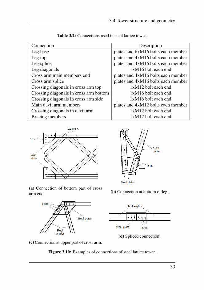
The connections used are listed in Table 3.2.
Examples of connections are illustrated in Figure 3.10. These are seenfrom one side only. For main members, angles will be fastened at bothflanges. The diagonal members will be fastened at one flange only. Wherepossible in regard to strength, only one bolt should be used at each end ofthe diagonal members to reduce the need for extra plates. The side crossingmembers below the davit arm need 2xM16 bolts and plates. Both the mainmembers of the legs and lower and upper cross arm will need to be spliced,like illustrated in Figure 3.10d.
According to FprEN 50341-1 (CENELEC, (2012)) overall maximum slen-derness for lattice steel legs is 150, which is maintained.
32
3.4 Tower structure and geometry
Table 3.2: Connections used in steel lattice tower.
Connection DescriptionLeg base plates and 6xM16 bolts each memberLeg top plates and 4xM16 bolts each memberLeg splice plates and 4xM16 bolts each memberLeg diagonals 1xM16 bolt each endCross arm main members end plates and 4xM16 bolts each memberCross arm splice plates and 4xM16 bolts each memberCrossing diagonals in cross arm top 1xM12 bolt each endCrossing diagonals in cross arm bottom 1xM16 bolt each endCrossing diagonals in cross arm side 1xM16 bolt each endMain davit arm members plates and 4xM12 bolts each memberCrossing diagonals in davit arm 1xM12 bolt each endBracing members 1xM12 bolt each end
(a) Connection of bottom part of crossarm end. (b) Connection at bottom of leg.
(c) Connection at upper part of cross arm.(d) Spliced connection.
Figure 3.10: Examples of connections of steel lattice tower.
33
Chapter 3. Design
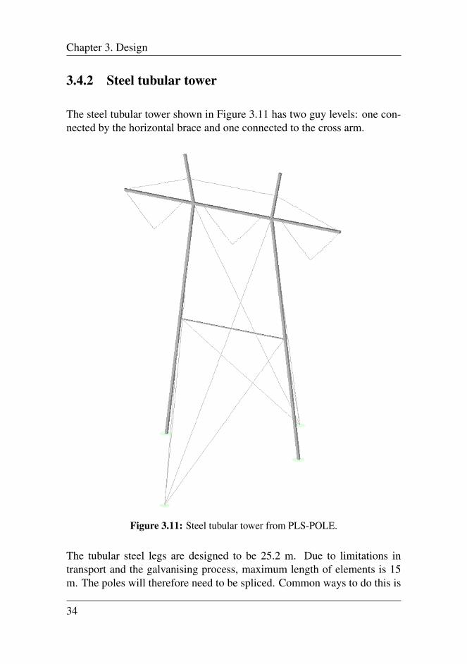
3.4.2 Steel tubular tower
The steel tubular tower shown in Figure 3.11 has two guy levels: one con-nected by the horizontal brace and one connected to the cross arm.
Figure 3.11: Steel tubular tower from PLS-POLE.
The tubular steel legs are designed to be 25.2 m. Due to limitations intransport and the galvanising process, maximum length of elements is 15m. The poles will therefore need to be spliced. Common ways to do this is
34
3.4 Tower structure and geometry
using either a slip joint or flange joint (Kiessling et al., (2003)) like shownin Figure 3.12.
(a) Slip joint.(b) Flange joint.
Figure 3.12: Examples of how to splice steel poles.
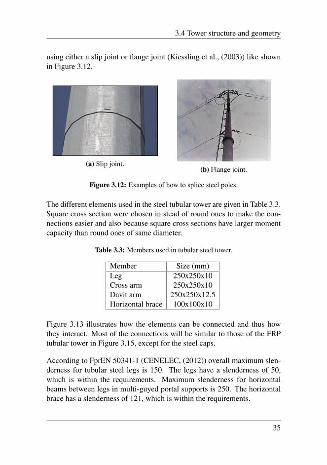
The different elements used in the steel tubular tower are given in Table 3.3.Square cross section were chosen in stead of round ones to make the con-nections easier and also because square cross sections have larger momentcapacity than round ones of same diameter.
Table 3.3: Members used in tubular steel tower.
Member Size (mm)Leg 250x250x10Cross arm 250x250x10Davit arm 250x250x12.5Horizontal brace 100x100x10
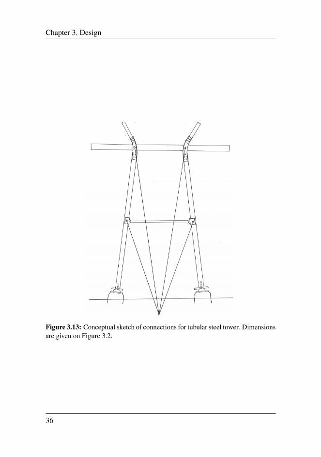
Figure 3.13 illustrates how the elements can be connected and thus howthey interact. Most of the connections will be similar to those of the FRPtubular tower in Figure 3.15, except for the steel caps.
According to FprEN 50341-1 (CENELEC, (2012)) overall maximum slen-derness for tubular steel legs is 150. The legs have a slenderness of 50,which is within the requirements. Maximum slenderness for horizontalbeams between legs in multi-guyed portal supports is 250. The horizontalbrace has a slenderness of 121, which is within the requirements.
35
Chapter 3. Design
Figure 3.13: Conceptual sketch of connections for tubular steel tower. Dimensionsare given on Figure 3.2.
36
3.4 Tower structure and geometry
3.4.3 FRP tubular tower
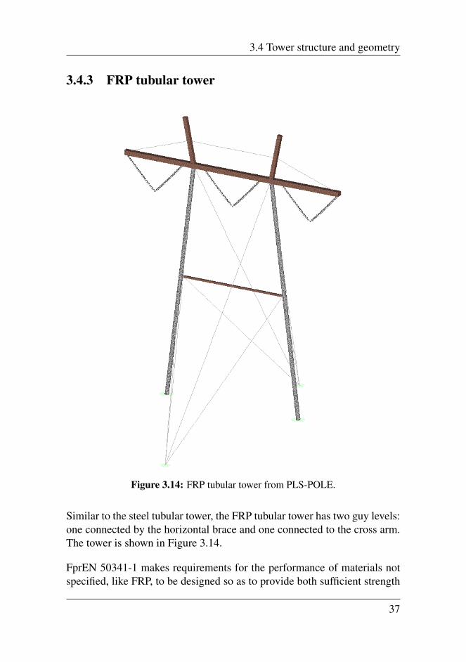
Figure 3.14: FRP tubular tower from PLS-POLE.
Similar to the steel tubular tower, the FRP tubular tower has two guy levels:one connected by the horizontal brace and one connected to the cross arm.The tower is shown in Figure 3.14.
FprEN 50341-1 makes requirements for the performance of materials notspecified, like FRP, to be designed so as to provide both sufficient strength
37
Chapter 3. Design
and serviceability (CENELEC, (2012)). As no particular
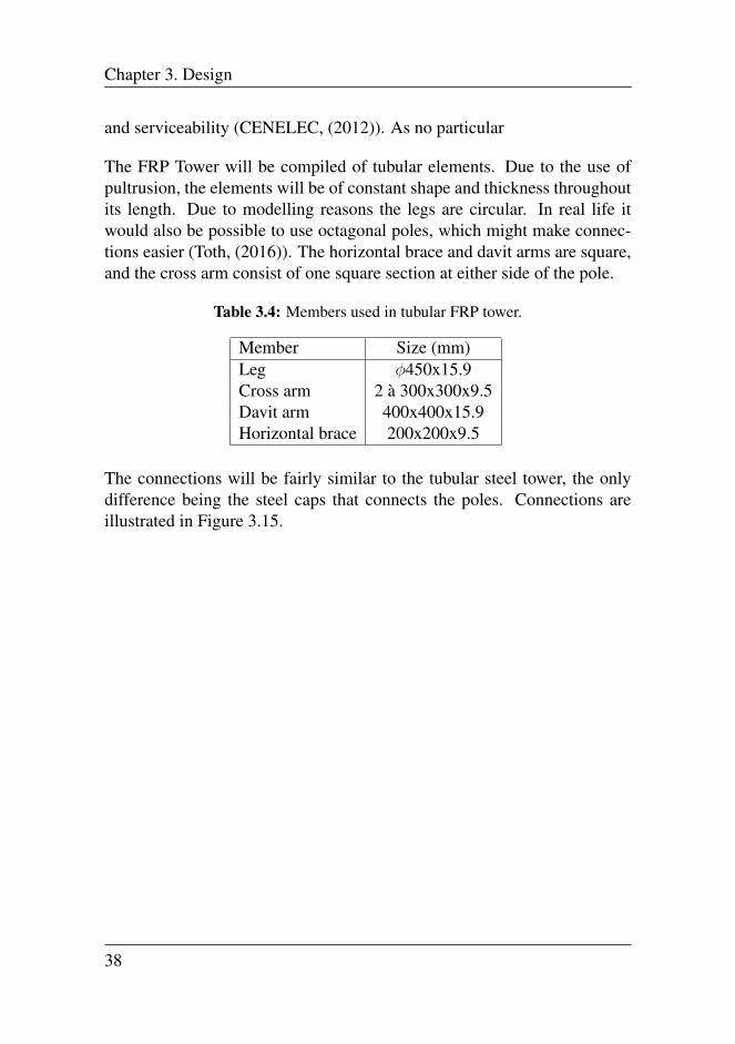
The FRP Tower will be compiled of tubular elements. Due to the use ofpultrusion, the elements will be of constant shape and thickness throughoutits length. Due to modelling reasons the legs are circular. In real life itwould also be possible to use octagonal poles, which might make connec-tions easier (Toth, (2016)). The horizontal brace and davit arms are square,and the cross arm consist of one square section at either side of the pole.
Table 3.4: Members used in tubular FRP tower.
Member Size (mm)Leg φ450x15.9Cross arm 2 a 300x300x9.5Davit arm 400x400x15.9Horizontal brace 200x200x9.5
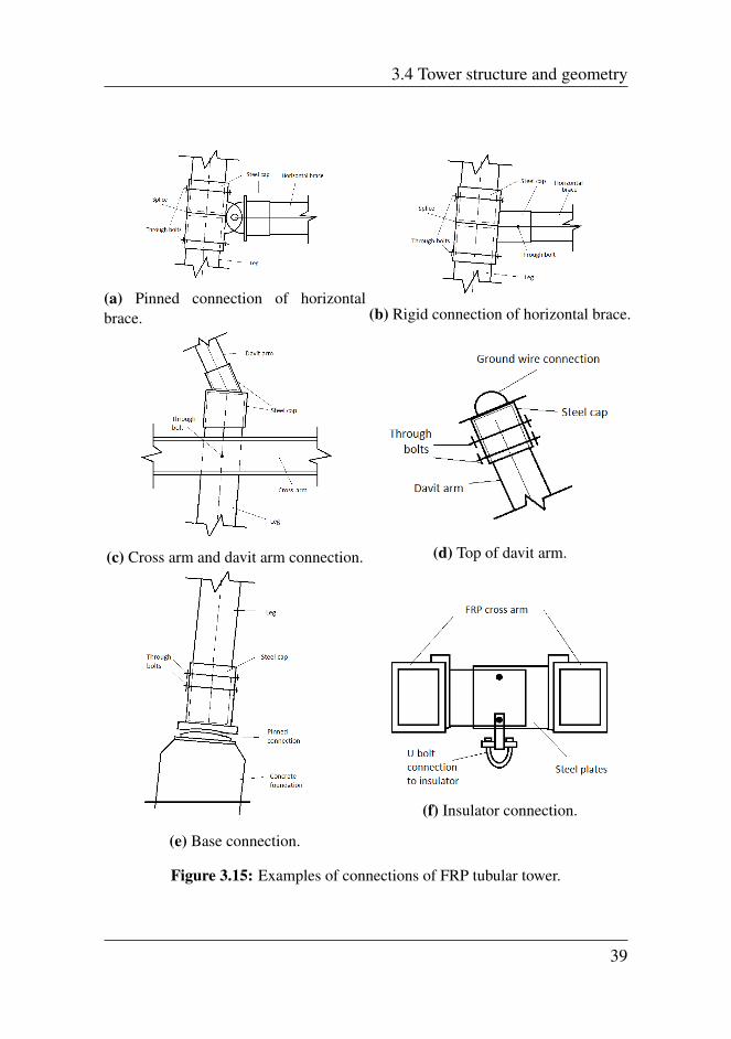
The connections will be fairly similar to the tubular steel tower, the onlydifference being the steel caps that connects the poles. Connections areillustrated in Figure 3.15.
38
3.4 Tower structure and geometry
(a) Pinned connection of horizontalbrace. (b) Rigid connection of horizontal brace.
(c) Cross arm and davit arm connection. (d) Top of davit arm.
(e) Base connection.
(f) Insulator connection.
Figure 3.15: Examples of connections of FRP tubular tower.
39

Chapter 4Actions on Lines
The standard FprEN 50341-1:2012 (CENELEC, (2012)) given by the Euro-pean Committee for Electrotechnical Standardization give guidance on howto calculate the loads on the lines and their components; such as insulatorsets, conductors, poles and lattice towers.
The loads affecting the transmission lines come from several sources andare in the design process given different amount of attention. The mostcritical ones are the ones due to environmental effects. Such as wind loads,ice loads and the effect of temperature on loads. Then come the loads dueto our actions, such as the construction or maintenance of the structure.Last there are the discrete events. These can be from natural sources, suchas earthquakes, landslides and avalanches, or from internal sources, likefailed components (Catchpole and Fife, (2014)).
These actions can also be classified by their duration where they are ei-ther permanent or variable. Permanent actions include the dead loads ofall components of the structure. Variable actions are often caused by cli-matic actions such as wind, ice or temperature changes. These are oftenreferred to as live loads. Accidental actions happen seldom and can refer toavalanches or component failures (CENELEC, (2012)).
Data used in these calculations can either be provided in standards, it canbe determined based on statistical data and field observations or it can be
41
Chapter 4. Actions on Lines
based on data calibrated from previous successful designs.
4.1 Dead load
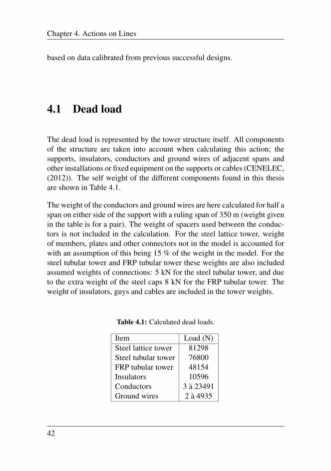
The dead load is represented by the tower structure itself. All componentsof the structure are taken into account when calculating this action; thesupports, insulators, conductors and ground wires of adjacent spans andother installations or fixed equipment on the supports or cables (CENELEC,(2012)). The self weight of the different components found in this thesisare shown in Table 4.1.
The weight of the conductors and ground wires are here calculated for half aspan on either side of the support with a ruling span of 350 m (weight givenin the table is for a pair). The weight of spacers used between the conduc-tors is not included in the calculation. For the steel lattice tower, weightof members, plates and other connectors not in the model is accounted forwith an assumption of this being 15 % of the weight in the model. For thesteel tubular tower and FRP tubular tower these weights are also includedassumed weights of connections: 5 kN for the steel tubular tower, and dueto the extra weight of the steel caps 8 kN for the FRP tubular tower. Theweight of insulators, guys and cables are included in the tower weights.
Table 4.1: Calculated dead loads.
Item Load (N)Steel lattice tower 81298Steel tubular tower 76800FRP tubular tower 48154Insulators 10596Conductors 3 a 23491Ground wires 2 a 4935
42
4.2 Temperature load
4.2 Temperature load
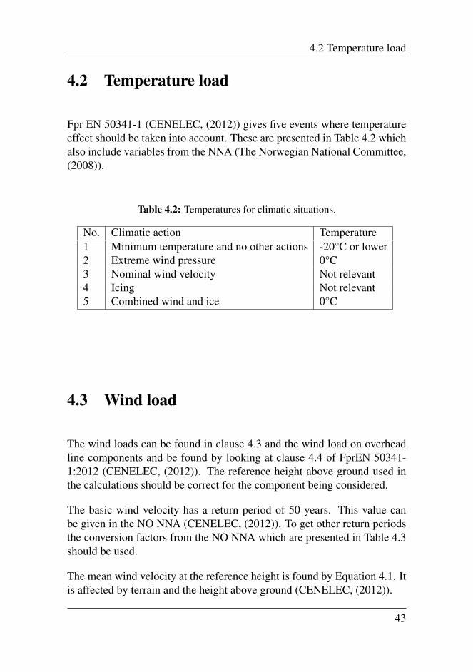
Fpr EN 50341-1 (CENELEC, (2012)) gives five events where temperatureeffect should be taken into account. These are presented in Table 4.2 whichalso include variables from the NNA (The Norwegian National Committee,(2008)).
Table 4.2: Temperatures for climatic situations.
No. Climatic action Temperature1 Minimum temperature and no other actions -20°C or lower2 Extreme wind pressure 0°C3 Nominal wind velocity Not relevant4 Icing Not relevant5 Combined wind and ice 0°C
4.3 Wind load
The wind loads can be found in clause 4.3 and the wind load on overheadline components and be found by looking at clause 4.4 of FprEN 50341-1:2012 (CENELEC, (2012)). The reference height above ground used inthe calculations should be correct for the component being considered.
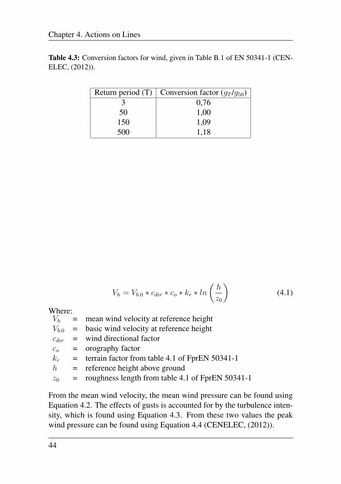
The basic wind velocity has a return period of 50 years. This value canbe given in the NO NNA (CENELEC, (2012)). To get other return periodsthe conversion factors from the NO NNA which are presented in Table 4.3should be used.
The mean wind velocity at the reference height is found by Equation 4.1. Itis affected by terrain and the height above ground (CENELEC, (2012)).
43
Chapter 4. Actions on Lines
Table 4.3: Conversion factors for wind, given in Table B.1 of EN 50341-1 (CEN-ELEC, (2012)).
Return period (T) Conversion factor (gT /g50)3 0,76
50 1,00150 1,09500 1,18
Vh = Vb.0 ∗ cdir ∗ co ∗ kr ∗ ln(h
z0
)(4.1)
Where:Vh = mean wind velocity at reference heightVb.0 = basic wind velocity at reference heightcdir = wind directional factorco = orography factorkr = terrain factor from table 4.1 of FprEN 50341-1h = reference height above groundz0 = roughness length from table 4.1 of FprEN 50341-1
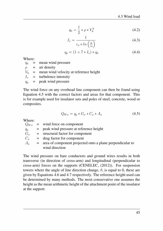
From the mean wind velocity, the mean wind pressure can be found usingEquation 4.2. The effects of gusts is accounted for by the turbulence inten-sity, which is found using Equation 4.3. From these two values the peakwind pressure can be found using Equation 4.4 (CENELEC, (2012)).
44
4.3 Wind load
qh =1
2∗ ρ ∗ V 2
h (4.2)
Iv =1
co ∗ ln(
hz0
) (4.3)
qp = (1 + 7 ∗ Iv) ∗ qh (4.4)
Where:qh = mean wind pressureρ = air densityVh = mean wind velocity at reference heightIv = turbulence intensityqp = peak wind pressure
The wind force on any overhead line component can then be found usingEquation 4.5 with the correct factors and areas for that component. Thisis for example used for insulator sets and poles of steel, concrete, wood orcomposites.
QWx = qp ∗Gx ∗ Cx ∗ Ax (4.5)
Where:QWx = wind force on componentqp = peak wind pressure at reference heightGx = structural factor for componentCx = drag factor for componentAx = area of component projected onto a plane perpendicular to
wind direction
The wind pressure on bare conductors and ground wires results in bothtransverse (in direction of cross-arm) and longitudinal (perpendicular tocross-arm) forces on the supports (CENELEC, (2012)). For suspensiontowers where the angle of line direction change, θ, is equal to 0, these aregiven by Equations 4.6 and 4.7 respectively. The reference height used canbe determined by many methods. The most conservative one assumes theheight as the mean arithmetic height of the attachment point of the insulatorat the support.
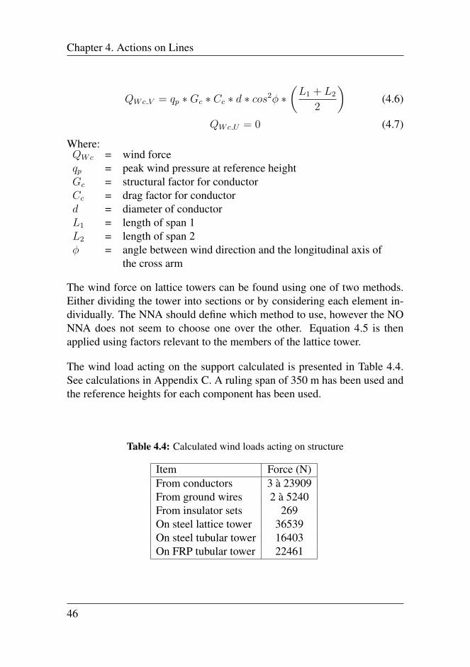
45
Chapter 4. Actions on Lines
QWc V = qp ∗Gc ∗ Cc ∗ d ∗ cos2φ ∗(L1 + L2
2
)(4.6)
QWc U = 0 (4.7)
Where:QWc = wind forceqp = peak wind pressure at reference heightGc = structural factor for conductorCc = drag factor for conductord = diameter of conductorL1 = length of span 1L2 = length of span 2φ = angle between wind direction and the longitudinal axis of
the cross arm
The wind force on lattice towers can be found using one of two methods.Either dividing the tower into sections or by considering each element in-dividually. The NNA should define which method to use, however the NONNA does not seem to choose one over the other. Equation 4.5 is thenapplied using factors relevant to the members of the lattice tower.
The wind load acting on the support calculated is presented in Table 4.4.See calculations in Appendix C. A ruling span of 350 m has been used andthe reference heights for each component has been used.
Table 4.4: Calculated wind loads acting on structure
Item Force (N)From conductors 3 a 23909From ground wires 2 a 5240From insulator sets 269On steel lattice tower 36539On steel tubular tower 16403On FRP tubular tower 22461
46
4.4 Ice load
4.4 Ice load
Ice on conductors will cause vertical forces on the structures and tension inthe conductors. The ice load on conductors, and as far as applicable on guywires, can be calculated by looking at clause 4.5 of FprEN 50341-1:2012(CENELEC, (2012)).
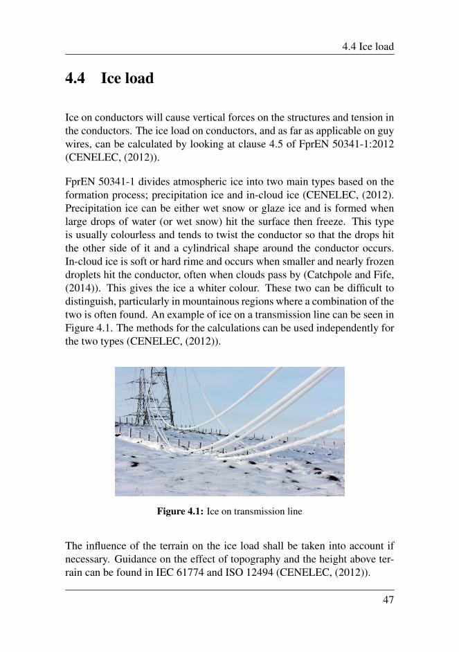
FprEN 50341-1 divides atmospheric ice into two main types based on theformation process; precipitation ice and in-cloud ice (CENELEC, (2012).Precipitation ice can be either wet snow or glaze ice and is formed whenlarge drops of water (or wet snow) hit the surface then freeze. This typeis usually colourless and tends to twist the conductor so that the drops hitthe other side of it and a cylindrical shape around the conductor occurs.In-cloud ice is soft or hard rime and occurs when smaller and nearly frozendroplets hit the conductor, often when clouds pass by (Catchpole and Fife,(2014)). This gives the ice a whiter colour. These two can be difficult todistinguish, particularly in mountainous regions where a combination of thetwo is often found. An example of ice on a transmission line can be seen inFigure 4.1. The methods for the calculations can be used independently forthe two types (CENELEC, (2012)).
Figure 4.1: Ice on transmission line
The influence of the terrain on the ice load shall be taken into account ifnecessary. Guidance on the effect of topography and the height above ter-rain can be found in IEC 61774 and ISO 12494 (CENELEC, (2012)).
47

Chapter 4. Actions on Lines
In places where the atmospheric and climatic conditions are varying alongthe overhead line, the line shall be divided into zones. This is done to getthe most accurate results possible (CENELEC, (2012)).
In many countries, the statistical data for ice is often poor. When that is thecase, the ice load must be based on experience (CENELEC, (2012)). ForNorway, data for some regions is given in clause 4.2.3.2 of the National An-nex (NA) (The Norwegian National Committee, (2008)). The values givenin the NA are presented in Table 4.5. For data concerning other regions, ameteorologist should be consulted.
Table 4.5: Design ice loads, given in Table 4.2.3.2/NO.1 of the NA (The Norwe-gian National Committee, (2008)).
No. Region Height above Design ice loadsea level (m) (N/m) 50 year
return period1 Main areas of the South East region* 0 - 200 302 Main areas of the South East region* 200 - 400 403 Main areas of the South East region 400 - 600 504 østfold and Vestfold 0 - 200 205 Telemark and Agder 0 - 200 356 Telemark and Agder 200 - 400 507 The coast Rogaland - Stad 0 - 200 358 The fjords Rogaland - Stad 0 - 400 409 The coast Stad - Namdalen 0 - 200 40
10 The fjords Stad - Namdalen 0 - 400 4011 The coast Namdalen - Lofoten 0 - 200 4012 The inland of Nordland 0 - 200 3013 The coast Vesteralen - Nordkapp 0 - 100 3514 The inland Troms - Vest-Finnmark 0 - 200 3015 The coast of Aust-Finnmark 0 - 100 3016 The inland of Aust-Finnmark 0 - 200 20
*Except areas mentioned in no 3 and 4.
To get the correct return period for the design loads, the conversion factors
48
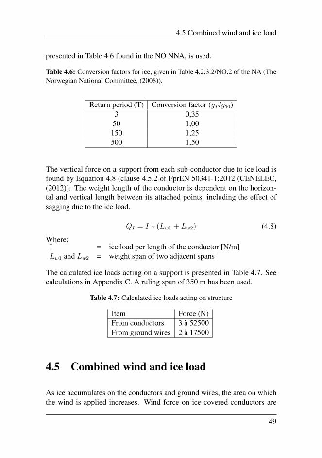
4.5 Combined wind and ice load
presented in Table 4.6 found in the NO NNA, is used.
Table 4.6: Conversion factors for ice, given in Table 4.2.3.2/NO.2 of the NA (TheNorwegian National Committee, (2008)).
Return period (T) Conversion factor (gT /g50)3 0,35
50 1,00150 1,25500 1,50
The vertical force on a support from each sub-conductor due to ice load isfound by Equation 4.8 (clause 4.5.2 of FprEN 50341-1:2012 (CENELEC,(2012)). The weight length of the conductor is dependent on the horizon-tal and vertical length between its attached points, including the effect ofsagging due to the ice load.
QI = I ∗ (Lw1 + Lw2) (4.8)
Where:I = ice load per length of the conductor [N/m]Lw1 and Lw2 = weight span of two adjacent spans
The calculated ice loads acting on a support is presented in Table 4.7. Seecalculations in Appendix C. A ruling span of 350 m has been used.
Table 4.7: Calculated ice loads acting on structure
Item Force (N)From conductors 3 a 52500From ground wires 2 a 17500
4.5 Combined wind and ice load
As ice accumulates on the conductors and ground wires, the area on whichthe wind is applied increases. Wind force on ice covered conductors are
49
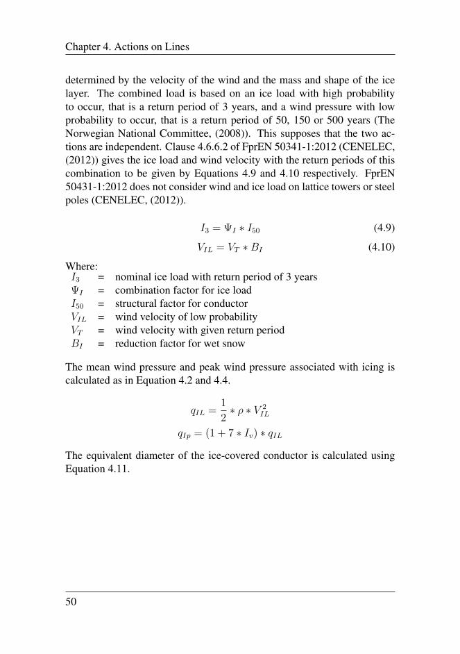
Chapter 4. Actions on Lines
determined by the velocity of the wind and the mass and shape of the icelayer. The combined load is based on an ice load with high probabilityto occur, that is a return period of 3 years, and a wind pressure with lowprobability to occur, that is a return period of 50, 150 or 500 years (TheNorwegian National Committee, (2008)). This supposes that the two ac-tions are independent. Clause 4.6.6.2 of FprEN 50341-1:2012 (CENELEC,(2012)) gives the ice load and wind velocity with the return periods of thiscombination to be given by Equations 4.9 and 4.10 respectively. FprEN50431-1:2012 does not consider wind and ice load on lattice towers or steelpoles (CENELEC, (2012)).
I3 = ΨI ∗ I50 (4.9)
VIL = VT ∗BI (4.10)
Where:I3 = nominal ice load with return period of 3 yearsΨI = combination factor for ice loadI50 = structural factor for conductorVIL = wind velocity of low probabilityVT = wind velocity with given return periodBI = reduction factor for wet snow
The mean wind pressure and peak wind pressure associated with icing iscalculated as in Equation 4.2 and 4.4.
qIL =1
2∗ ρ ∗ V 2
IL
qIp = (1 + 7 ∗ Iv) ∗ qIL
The equivalent diameter of the ice-covered conductor is calculated usingEquation 4.11.
50
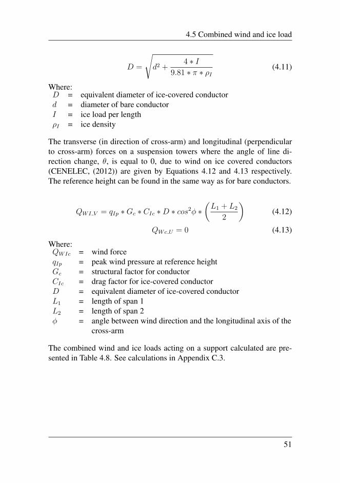
4.5 Combined wind and ice load
D =
√d2 +
4 ∗ I9.81 ∗ π ∗ ρI
(4.11)
Where:D = equivalent diameter of ice-covered conductord = diameter of bare conductorI = ice load per lengthρI = ice density
The transverse (in direction of cross-arm) and longitudinal (perpendicularto cross-arm) forces on a suspension towers where the angle of line di-rection change, θ, is equal to 0, due to wind on ice covered conductors(CENELEC, (2012)) are given by Equations 4.12 and 4.13 respectively.The reference height can be found in the same way as for bare conductors.
QWI V = qIp ∗Gc ∗ CIc ∗D ∗ cos2φ ∗(L1 + L2
2
)(4.12)
QWc U = 0 (4.13)
Where:QWIc = wind forceqIp = peak wind pressure at reference heightGc = structural factor for conductorCIc = drag factor for ice-covered conductorD = equivalent diameter of ice-covered conductorL1 = length of span 1L2 = length of span 2φ = angle between wind direction and the longitudinal axis of the
cross-arm
The combined wind and ice loads acting on a support calculated are pre-sented in Table 4.8. See calculations in Appendix C.3.
51
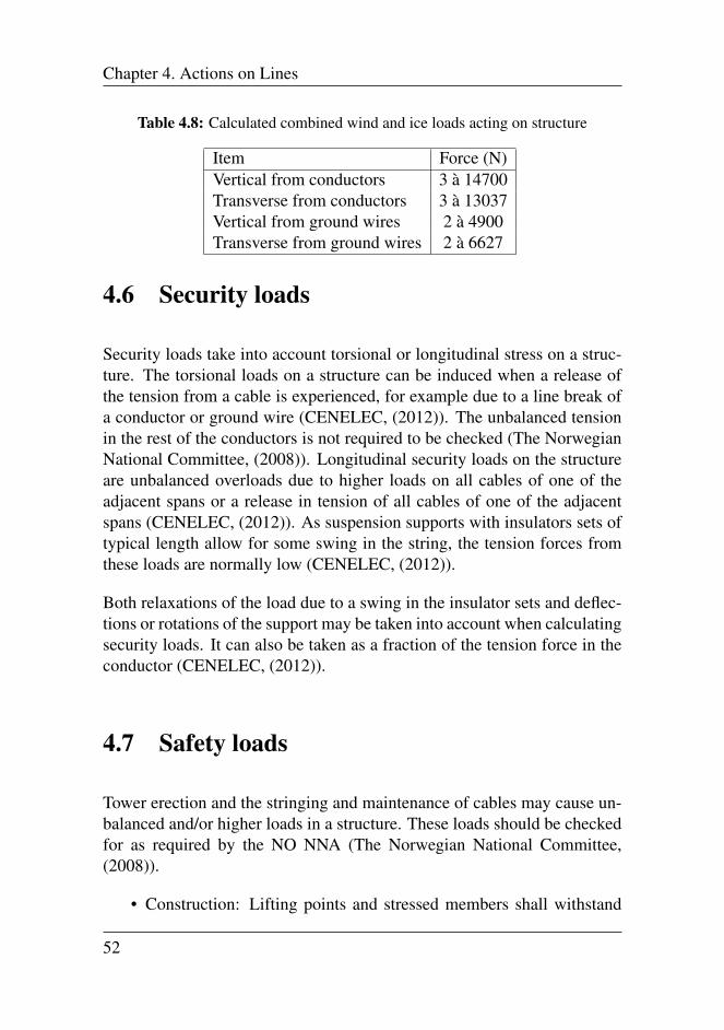
Chapter 4. Actions on Lines
Table 4.8: Calculated combined wind and ice loads acting on structure
Item Force (N)Vertical from conductors 3 a 14700Transverse from conductors 3 a 13037Vertical from ground wires 2 a 4900Transverse from ground wires 2 a 6627
4.6 Security loads
Security loads take into account torsional or longitudinal stress on a struc-ture. The torsional loads on a structure can be induced when a release ofthe tension from a cable is experienced, for example due to a line break ofa conductor or ground wire (CENELEC, (2012)). The unbalanced tensionin the rest of the conductors is not required to be checked (The NorwegianNational Committee, (2008)). Longitudinal security loads on the structureare unbalanced overloads due to higher loads on all cables of one of theadjacent spans or a release in tension of all cables of one of the adjacentspans (CENELEC, (2012)). As suspension supports with insulators sets oftypical length allow for some swing in the string, the tension forces fromthese loads are normally low (CENELEC, (2012)).
Both relaxations of the load due to a swing in the insulator sets and deflec-tions or rotations of the support may be taken into account when calculatingsecurity loads. It can also be taken as a fraction of the tension force in theconductor (CENELEC, (2012)).
4.7 Safety loads
Tower erection and the stringing and maintenance of cables may cause un-balanced and/or higher loads in a structure. These loads should be checkedfor as required by the NO NNA (The Norwegian National Committee,(2008)).
• Construction: Lifting points and stressed members shall withstand
52
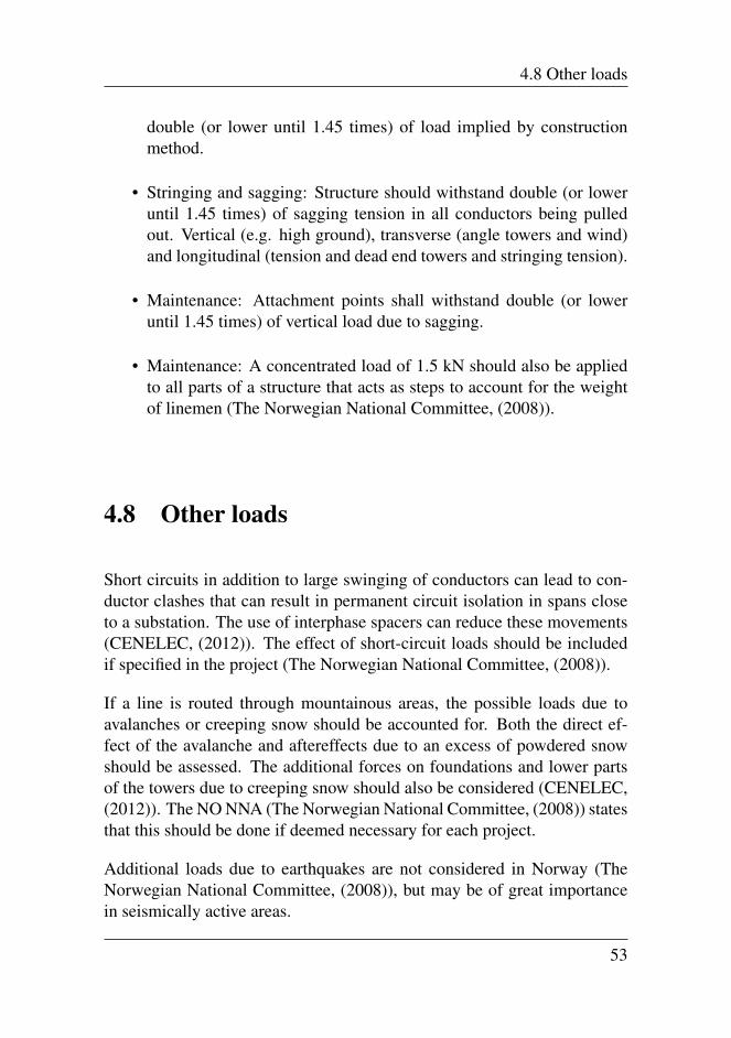
4.8 Other loads
double (or lower until 1.45 times) of load implied by constructionmethod.
• Stringing and sagging: Structure should withstand double (or loweruntil 1.45 times) of sagging tension in all conductors being pulledout. Vertical (e.g. high ground), transverse (angle towers and wind)and longitudinal (tension and dead end towers and stringing tension).
• Maintenance: Attachment points shall withstand double (or loweruntil 1.45 times) of vertical load due to sagging.
• Maintenance: A concentrated load of 1.5 kN should also be appliedto all parts of a structure that acts as steps to account for the weightof linemen (The Norwegian National Committee, (2008)).
4.8 Other loads
Short circuits in addition to large swinging of conductors can lead to con-ductor clashes that can result in permanent circuit isolation in spans closeto a substation. The use of interphase spacers can reduce these movements(CENELEC, (2012)). The effect of short-circuit loads should be includedif specified in the project (The Norwegian National Committee, (2008)).
If a line is routed through mountainous areas, the possible loads due toavalanches or creeping snow should be accounted for. Both the direct ef-fect of the avalanche and aftereffects due to an excess of powdered snowshould be assessed. The additional forces on foundations and lower partsof the towers due to creeping snow should also be considered (CENELEC,(2012)). The NO NNA (The Norwegian National Committee, (2008)) statesthat this should be done if deemed necessary for each project.
Additional loads due to earthquakes are not considered in Norway (TheNorwegian National Committee, (2008)), but may be of great importancein seismically active areas.
53
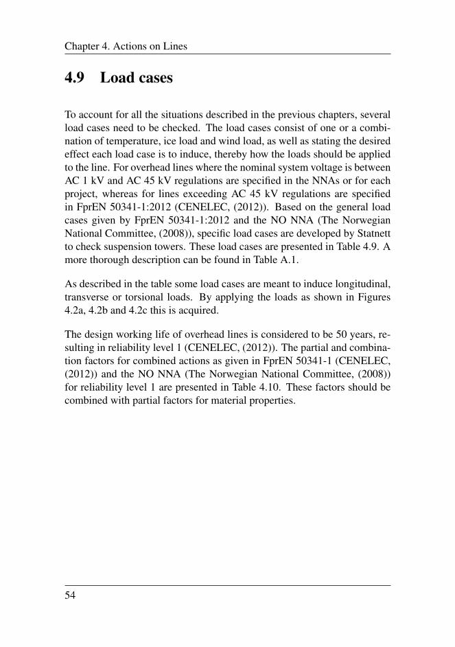
Chapter 4. Actions on Lines
4.9 Load cases
To account for all the situations described in the previous chapters, severalload cases need to be checked. The load cases consist of one or a combi-nation of temperature, ice load and wind load, as well as stating the desiredeffect each load case is to induce, thereby how the loads should be appliedto the line. For overhead lines where the nominal system voltage is betweenAC 1 kV and AC 45 kV regulations are specified in the NNAs or for eachproject, whereas for lines exceeding AC 45 kV regulations are specifiedin FprEN 50341-1:2012 (CENELEC, (2012)). Based on the general loadcases given by FprEN 50341-1:2012 and the NO NNA (The NorwegianNational Committee, (2008)), specific load cases are developed by Statnettto check suspension towers. These load cases are presented in Table 4.9. Amore thorough description can be found in Table A.1.
As described in the table some load cases are meant to induce longitudinal,transverse or torsional loads. By applying the loads as shown in Figures4.2a, 4.2b and 4.2c this is acquired.
The design working life of overhead lines is considered to be 50 years, re-sulting in reliability level 1 (CENELEC, (2012)). The partial and combina-tion factors for combined actions as given in FprEN 50341-1 (CENELEC,(2012)) and the NO NNA (The Norwegian National Committee, (2008))for reliability level 1 are presented in Table 4.10. These factors should becombined with partial factors for material properties.
54

4.9 Load cases
Table 4.9: Load cases used in model
No. Description0 EDS1 Full ice load2 Uneven ice load - Transverse bending towards the right3 Uneven ice load - Transverse bending towards the left4 Uneven ice load previous span5 Uneven ice load next span6 Uneven ice load previous span - Transverse bending towards the
right7 Uneven ice load previous span - Transverse bending towards the
left8 Uneven ice load next span - Transverse bending towards the right9 Uneven ice load next span - Transverse bending towards the left10 Wind on line towards the right11 Wind on line towards the left12 Wind on ice loaded line towards the right13 Wind on ice loaded line towards the left14 Minimum temperature15 Line break left phase of next span16 Line break left phase of previous span17 Line break middle phase of next span18 Line break middle phase of previous span19 Line break right phase of next span20 Line break right phase of previous span21 Line break left ground wire of next span22 Line break left ground wire of previous span23 Line break right ground wire of next span24 Line break right ground wire of previous span
55
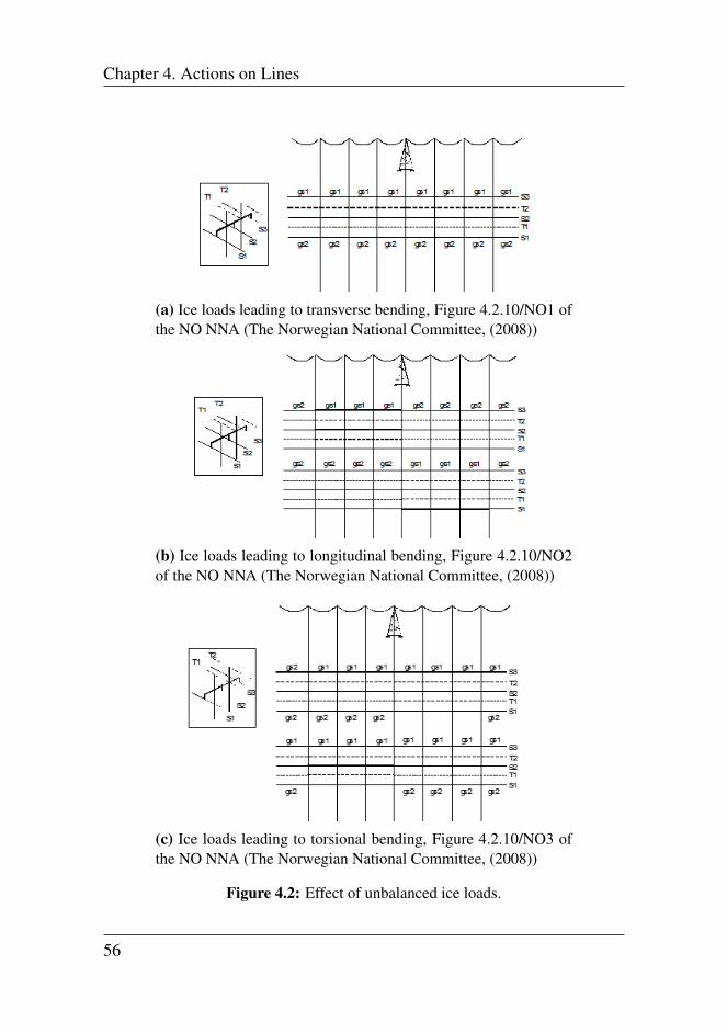
Chapter 4. Actions on Lines
(a) Ice loads leading to transverse bending, Figure 4.2.10/NO1 ofthe NO NNA (The Norwegian National Committee, (2008))
(b) Ice loads leading to longitudinal bending, Figure 4.2.10/NO2of the NO NNA (The Norwegian National Committee, (2008))
(c) Ice loads leading to torsional bending, Figure 4.2.10/NO3 ofthe NO NNA (The Norwegian National Committee, (2008))
Figure 4.2: Effect of unbalanced ice loads.
56
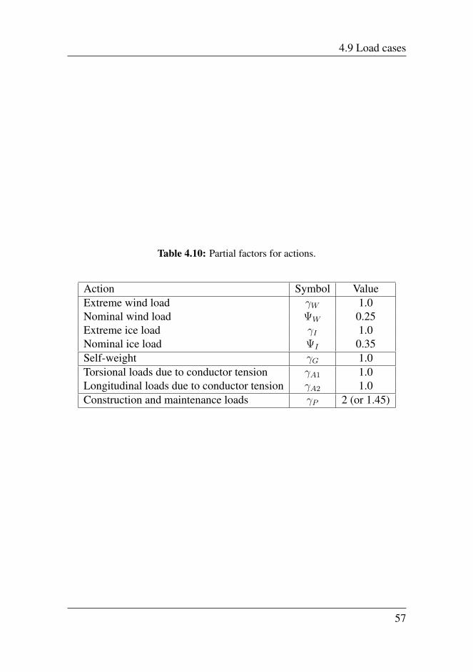
4.9 Load cases
Table 4.10: Partial factors for actions.
Action Symbol ValueExtreme wind load γW 1.0Nominal wind load ΨW 0.25Extreme ice load γI 1.0Nominal ice load ΨI 0.35Self-weight γG 1.0Torsional loads due to conductor tension γA1 1.0Longitudinal loads due to conductor tension γA2 1.0Construction and maintenance loads γP 2 (or 1.45)
57

Chapter 5Modelling
All modelling is done according to FprEN 50341-1 and the NO NNA andby help of the user’s manuals for the different programs.
The modelling of the line is done in PLS-CADD. This program enables theuser to route and design the line as well as conduct structure checks and ten-sion and sag calculations based on criteria input to account for all loadingsituations described in Chapter 4 (Power Line Systems Inc4, (2016).
The steel lattice tower is modelled using PLS-TOWER, while the steeltubular tower and FRP tubular tower are modelled using PLS-POLE.
By connecting the detailed models to PLS-CADD, the calculated loads areapplied to the structures and several outputs depicting for example stressesand usage are attained. Optimisation of the structures by reducing or in-creasing sizes where needed is then easily visualised.
Before modelling, some preliminary calculations were done to find somecross sections to begin with. This is explained further in 6.1.
After the modelling was done, the cross sections were optimised so thattheir strength was utilised as much as possible.
59
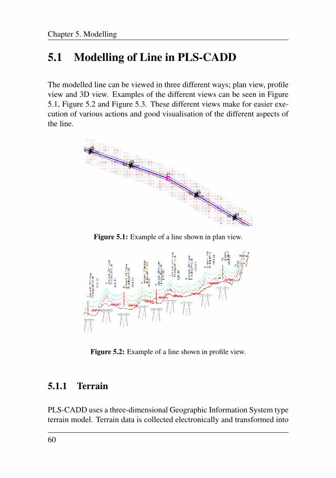
Chapter 5. Modelling
5.1 Modelling of Line in PLS-CADD
The modelled line can be viewed in three different ways; plan view, profileview and 3D view. Examples of the different views can be seen in Figure5.1, Figure 5.2 and Figure 5.3. These different views make for easier exe-cution of various actions and good visualisation of the different aspects ofthe line.
Figure 5.1: Example of a line shown in plan view.
Figure 5.2: Example of a line shown in profile view.
5.1.1 Terrain
PLS-CADD uses a three-dimensional Geographic Information System typeterrain model. Terrain data is collected electronically and transformed into
60
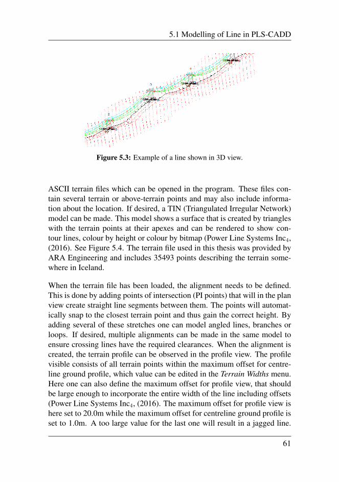
5.1 Modelling of Line in PLS-CADD
Figure 5.3: Example of a line shown in 3D view.
ASCII terrain files which can be opened in the program. These files con-tain several terrain or above-terrain points and may also include informa-tion about the location. If desired, a TIN (Triangulated Irregular Network)model can be made. This model shows a surface that is created by triangleswith the terrain points at their apexes and can be rendered to show con-tour lines, colour by height or colour by bitmap (Power Line Systems Inc4,(2016). See Figure 5.4. The terrain file used in this thesis was provided byARA Engineering and includes 35493 points describing the terrain some-where in Iceland.
When the terrain file has been loaded, the alignment needs to be defined.This is done by adding points of intersection (PI points) that will in the planview create straight line segments between them. The points will automat-ically snap to the closest terrain point and thus gain the correct height. Byadding several of these stretches one can model angled lines, branches orloops. If desired, multiple alignments can be made in the same model toensure crossing lines have the required clearances. When the alignment iscreated, the terrain profile can be observed in the profile view. The profilevisible consists of all terrain points within the maximum offset for centre-line ground profile, which value can be edited in the Terrain Widths menu.Here one can also define the maximum offset for profile view, that shouldbe large enough to incorporate the entire width of the line including offsets(Power Line Systems Inc4, (2016). The maximum offset for profile view ishere set to 20.0m while the maximum offset for centreline ground profile isset to 1.0m. A too large value for the last one will result in a jagged line.
61
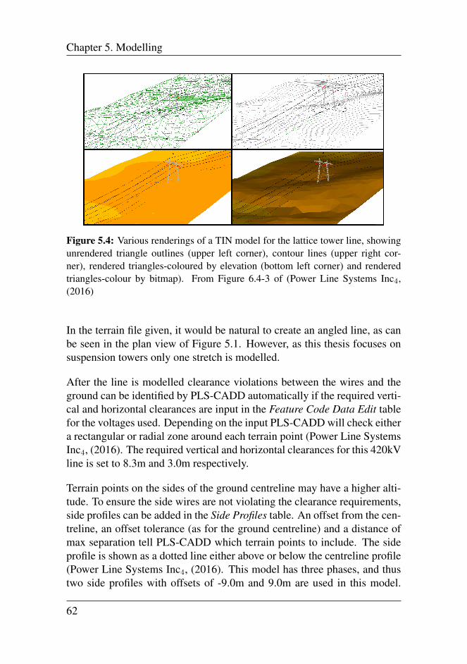
Chapter 5. Modelling
Figure 5.4: Various renderings of a TIN model for the lattice tower line, showingunrendered triangle outlines (upper left corner), contour lines (upper right cor-ner), rendered triangles-coloured by elevation (bottom left corner) and renderedtriangles-colour by bitmap). From Figure 6.4-3 of (Power Line Systems Inc4,(2016)
In the terrain file given, it would be natural to create an angled line, as canbe seen in the plan view of Figure 5.1. However, as this thesis focuses onsuspension towers only one stretch is modelled.
After the line is modelled clearance violations between the wires and theground can be identified by PLS-CADD automatically if the required verti-cal and horizontal clearances are input in the Feature Code Data Edit tablefor the voltages used. Depending on the input PLS-CADD will check eithera rectangular or radial zone around each terrain point (Power Line SystemsInc4, (2016). The required vertical and horizontal clearances for this 420kVline is set to 8.3m and 3.0m respectively.
Terrain points on the sides of the ground centreline may have a higher alti-tude. To ensure the side wires are not violating the clearance requirements,side profiles can be added in the Side Profiles table. An offset from the cen-treline, an offset tolerance (as for the ground centreline) and a distance ofmax separation tell PLS-CADD which terrain points to include. The sideprofile is shown as a dotted line either above or below the centreline profile(Power Line Systems Inc4, (2016). This model has three phases, and thustwo side profiles with offsets of -9.0m and 9.0m are used in this model.
62
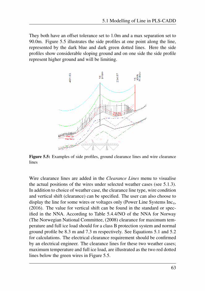
5.1 Modelling of Line in PLS-CADD
They both have an offset tolerance set to 1.0m and a max separation set to90.0m. Figure 5.5 illustrates the side profiles at one point along the line,represented by the dark blue and dark green dotted lines. Here the sideprofiles show considerable sloping ground and on one side the side profilerepresent higher ground and will be limiting.
Figure 5.5: Examples of side profiles, ground clearance lines and wire clearancelines
Wire clearance lines are added in the Clearance Lines menu to visualisethe actual positions of the wires under selected weather cases (see 5.1.3).In addition to choice of weather case, the clearance line type, wire conditionand vertical shift (clearance) can be specified. The user can also choose todisplay the line for some wires or voltages only (Power Line Systems Inc4,(2016). The value for vertical shift can be found in the standard or spec-ified in the NNA. According to Table 5.4.4/NO of the NNA for Norway(The Norwegian National Committee, (2008) clearance for maximum tem-perature and full ice load should for a class B protection system and normalground profile be 8.3 m and 7.3 m respectively. See Equations 5.1 and 5.2for calculations. The electrical clearance requirement should be confirmedby an electrical engineer. The clearance lines for these two weather cases;maximum temperature and full ice load, are illustrated as the two red dottedlines below the green wires in Figure 5.5.
63
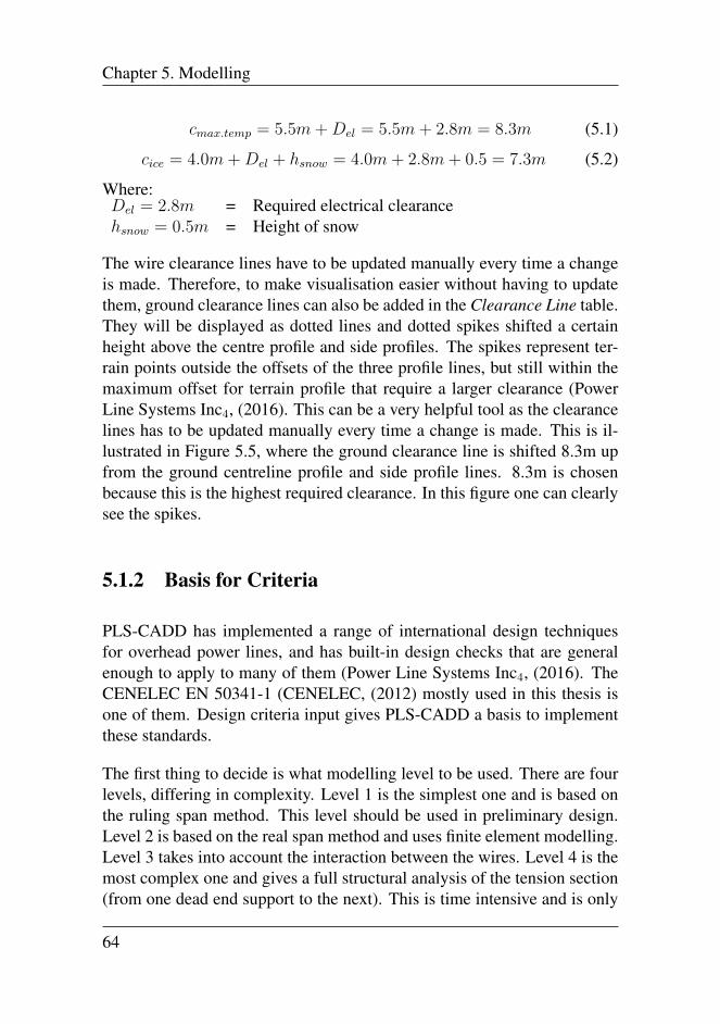
Chapter 5. Modelling
cmax.temp = 5.5m+Del = 5.5m+ 2.8m = 8.3m (5.1)
cice = 4.0m+Del + hsnow = 4.0m+ 2.8m+ 0.5 = 7.3m (5.2)
Where:Del = 2.8m = Required electrical clearancehsnow = 0.5m = Height of snow
The wire clearance lines have to be updated manually every time a changeis made. Therefore, to make visualisation easier without having to updatethem, ground clearance lines can also be added in the Clearance Line table.They will be displayed as dotted lines and dotted spikes shifted a certainheight above the centre profile and side profiles. The spikes represent ter-rain points outside the offsets of the three profile lines, but still within themaximum offset for terrain profile that require a larger clearance (PowerLine Systems Inc4, (2016). This can be a very helpful tool as the clearancelines has to be updated manually every time a change is made. This is il-lustrated in Figure 5.5, where the ground clearance line is shifted 8.3m upfrom the ground centreline profile and side profile lines. 8.3m is chosenbecause this is the highest required clearance. In this figure one can clearlysee the spikes.
5.1.2 Basis for Criteria
PLS-CADD has implemented a range of international design techniquesfor overhead power lines, and has built-in design checks that are generalenough to apply to many of them (Power Line Systems Inc4, (2016). TheCENELEC EN 50341-1 (CENELEC, (2012) mostly used in this thesis isone of them. Design criteria input gives PLS-CADD a basis to implementthese standards.
The first thing to decide is what modelling level to be used. There are fourlevels, differing in complexity. Level 1 is the simplest one and is based onthe ruling span method. This level should be used in preliminary design.Level 2 is based on the real span method and uses finite element modelling.Level 3 takes into account the interaction between the wires. Level 4 is themost complex one and gives a full structural analysis of the tension section(from one dead end support to the next). This is time intensive and is only
64
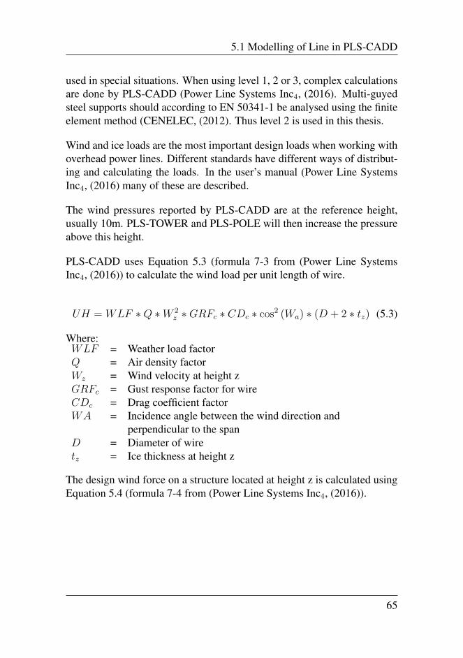
5.1 Modelling of Line in PLS-CADD
used in special situations. When using level 1, 2 or 3, complex calculationsare done by PLS-CADD (Power Line Systems Inc4, (2016). Multi-guyedsteel supports should according to EN 50341-1 be analysed using the finiteelement method (CENELEC, (2012). Thus level 2 is used in this thesis.
Wind and ice loads are the most important design loads when working withoverhead power lines. Different standards have different ways of distribut-ing and calculating the loads. In the user’s manual (Power Line SystemsInc4, (2016) many of these are described.
The wind pressures reported by PLS-CADD are at the reference height,usually 10m. PLS-TOWER and PLS-POLE will then increase the pressureabove this height.
PLS-CADD uses Equation 5.3 (formula 7-3 from (Power Line SystemsInc4, (2016)) to calculate the wind load per unit length of wire.
UH = WLF ∗Q ∗W 2z ∗GRFc ∗ CDc ∗ cos2 (Wa) ∗ (D + 2 ∗ tz) (5.3)
Where:WLF = Weather load factorQ = Air density factorWz = Wind velocity at height zGRFc = Gust response factor for wireCDc = Drag coefficient factorWA = Incidence angle between the wind direction and
perpendicular to the spanD = Diameter of wiretz = Ice thickness at height z
The design wind force on a structure located at height z is calculated usingEquation 5.4 (formula 7-4 from (Power Line Systems Inc4, (2016)).
65
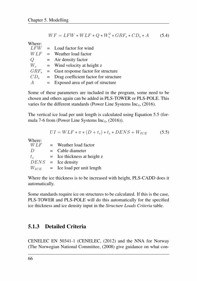
Chapter 5. Modelling
WF = LFW ∗WLF ∗Q ∗W 2z ∗GRFs ∗ CDs ∗ A (5.4)
Where:LFW = Load factor for windWLF = Weather load factorQ = Air density factorWz = Wind velocity at height zGRFs = Gust response factor for structureCDs = Drag coefficient factor for structureA = Exposed area of part of structure
Some of these parameters are included in the program, some need to bechosen and others again can be added in PLS-TOWER or PLS-POLE. Thisvaries for the different standards (Power Line Systems Inc4, (2016).
The vertical ice load per unit length is calculated using Equation 5.5 (for-mula 7-6 from (Power Line Systems Inc4, (2016)).
UI = WLF ∗ π ∗ (D + tz) ∗ tz ∗DENS +WICE (5.5)
Where:WLF = Weather load factorD = Cable diametertz = Ice thickness at height zDENS = Ice densityWICE = Ice load per unit length
Where the ice thickness is to be increased with height, PLS-CADD does itautomatically.
Some standards require ice on structures to be calculated. If this is the case,PLS-TOWER and PLS-POLE will do this automatically for the specifiedice thickness and ice density input in the Structure Loads Criteria table.
5.1.3 Detailed Criteria
CENELEC EN 50341-1 (CENELEC, (2012) and the NNA for Norway(The Norwegian National Committee, (2008) give guidance on what con-
66
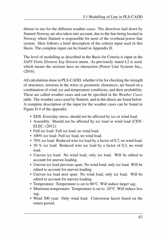
5.1 Modelling of Line in PLS-CADD
ditions to use for the different weather cases. The directives laid down byStatnett Norway are also taken into account, due to the line being located inNorway where Statnett is responsible for most of the overhead power linesystem. Here follows a brief description of the criteria input used in thisthesis. The complete input can be found in Appendix II.
The level of modelling as described in the Basis for Criteria is input in theSAPS Finite Element Sag-Tension menu. As previously stated L2 is used,which means the sections have no interaction (Power Line Systems Inc4,(2016).
All calculations done in PLS-CADD, whether it be for checking the strengthof structures, tensions in the wires or geometric clearances, are based on acombination of wind, ice and temperature conditions, and their probability.These are called weather cases and can be specified in the Weather Casestable. The weather cases used by Statnett, and in this thesis are listed below.A complete description of the input for the weather cases can be found inFigure D.4 of the appendix.
• EDS: Everyday stress, should not be affected by ice or wind load.• Assembly: Should not be affected by ice load or wind load (CEN-
ELEC, (2012).• Full ice load: Full ice load, no wind load.• 100% ice load: Full ice load, no wind load.• 70% ice load: Reduced wire ice load by a factor of 0,7, no wind load.• 30 % ice load: Reduced wire ice load by a factor of 0,3, no wind
load.• Uneven ice load: No wind load, only ice load. Will be edited to
account for uneven loading.• Uneven ice load previous span: No wind load, only ice load. Will be
edited to account for uneven loading.• Uneven ice load next span: No wind load, only ice load. Will be
edited to account for uneven loading.• Temperature: Temperature is set to 80°C. Will induce larger sag.• Minimum temperature: Temperature is set to -20°C. Will induce less
sag.• Wind 500 year: Only wind load. Conversion factor based on the
return period.
67
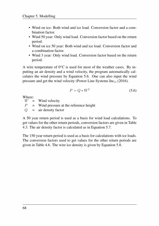
Chapter 5. Modelling
• Wind on ice: Both wind and ice load. Conversion factor and a com-bination factor.
• Wind 50 year: Only wind load. Conversion factor based on the returnperiod.
• Wind on ice 50 year: Both wind and ice load. Conversion factor anda combination factor.
• Wind 3 year: Only wind load. Conversion factor based on the returnperiod.
A wire temperature of 0°C is used for most of the weather cases. By in-putting an air density and a wind velocity, the program automatically cal-culates the wind pressure by Equation 5.6. One can also input the windpressure and get the wind velocity (Power Line Systems Inc4, (2016).
P = Q ∗W 2 (5.6)
Where:W = Wind velocityP = Wind pressure at the reference heightQ = air density factor
A 50 year return period is used as a basis for wind load calculations. Toget values for the other return periods, conversion factors are given in Table4.3. The air density factor is calculated as in Equation 5.7.
The 150 year return period is used as a basis for calculations with ice loads.The conversion factors used to get values for the other return periods aregiven in Table 4.6. The wire ice density is given by Equation 5.8.
68
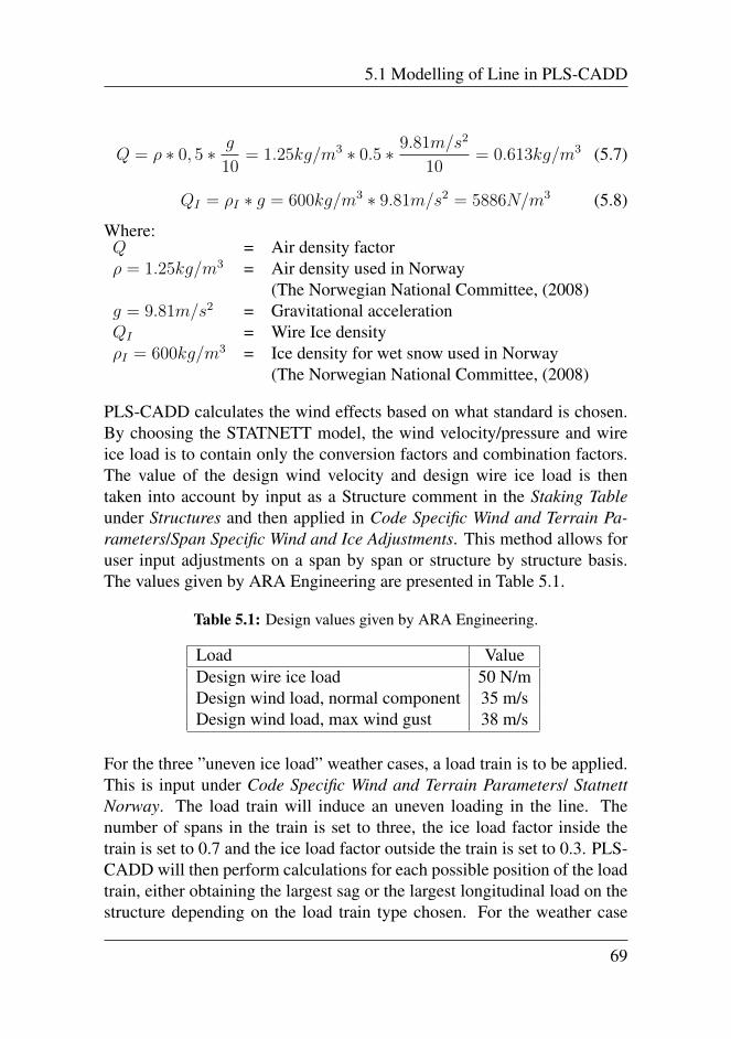
5.1 Modelling of Line in PLS-CADD
Q = ρ ∗ 0, 5 ∗ g
10= 1.25kg/m3 ∗ 0.5 ∗ 9.81m/s2
10= 0.613kg/m3 (5.7)
QI = ρI ∗ g = 600kg/m3 ∗ 9.81m/s2 = 5886N/m3 (5.8)
Where:Q = Air density factorρ = 1.25kg/m3 = Air density used in Norway
(The Norwegian National Committee, (2008)g = 9.81m/s2 = Gravitational accelerationQI = Wire Ice densityρI = 600kg/m3 = Ice density for wet snow used in Norway
(The Norwegian National Committee, (2008)
PLS-CADD calculates the wind effects based on what standard is chosen.By choosing the STATNETT model, the wind velocity/pressure and wireice load is to contain only the conversion factors and combination factors.The value of the design wind velocity and design wire ice load is thentaken into account by input as a Structure comment in the Staking Tableunder Structures and then applied in Code Specific Wind and Terrain Pa-rameters/Span Specific Wind and Ice Adjustments. This method allows foruser input adjustments on a span by span or structure by structure basis.The values given by ARA Engineering are presented in Table 5.1.
Table 5.1: Design values given by ARA Engineering.
Load ValueDesign wire ice load 50 N/mDesign wind load, normal component 35 m/sDesign wind load, max wind gust 38 m/s
For the three ”uneven ice load” weather cases, a load train is to be applied.This is input under Code Specific Wind and Terrain Parameters/ StatnettNorway. The load train will induce an uneven loading in the line. Thenumber of spans in the train is set to three, the ice load factor inside thetrain is set to 0.7 and the ice load factor outside the train is set to 0.3. PLS-CADD will then perform calculations for each possible position of the loadtrain, either obtaining the largest sag or the largest longitudinal load on thestructure depending on the load train type chosen. For the weather case
69
Chapter 5. Modelling
”uneven ice load” the type ”max sag load train” is used, and for weathercases ”uneven ice load previous span” and ”uneven ice load next span” the”structure loads load train” type is used with ”max positive longitudinalload” and ”max negative longitudinal load” respectively.
PLS-CADD calculates the tension and sag of a cable for three conditions;initial, final after creep and final after load. The final after creep condi-tion originates in everyday stress in the cable over long time, thus inducingcreep. Short exposure to extreme load may lead to permanent stretches ofthe cable, thus the final after load condition is used. The weather cases usedfor these two conditions are specified in the Weather Cases for PermanentStretch Due to Creep and Load table (Power Line Systems Inc4, (2016).For final after creep the EDS weather case is used, and for the final afterload the full ice load weather case is used.
PLS-CADD also offers a choice for the aluminium outer part of the cable,whether it can take compression at high temperature or not. Due to alu-minium having a higher thermal expansion factor than steel it will at sometemperature no longer be under tension. This choice can be made in theBimetallic Conductor Model menu (Power Line Systems Inc4, (2016). Inthis thesis it is chosen to not have aluminium take compression.
Design limits for the ground wires and conductors are specified in the CableTensions table for different weather cases. In addition to weather case,the cable condition and a maximum tension either as a percentage or asa max value for tension or catenary has to be input. It is also possibleto choose which wires to apply these limits to (Power Line Systems Inc4,(2016). In this thesis the limits for all cables are set to 80% of ultimatetension for all weather cases chosen. The actual geometry of the wires areused to calculate the maximum tension. Another option is to calculate themaximum tension of the ruling span with equal and elevations. This ischosen in the Maximum Tension Criteria table (Power Line Systems Inc4,(2016).
There are four ways PLS-CADD checks the strength of structures, see5.1.4. Method 1 is defined in the Weight Span Model and Weight SpanCriteria (Method 1) menus. The interaction diagrams for method 2 can beedited in the Interaction Diagram Criteria (Method 2) table. Methods 3
70
5.1 Modelling of Line in PLS-CADD
and 4 are based on load cases defined in the Structure Loads (Method 3,4)table. Method 4 structures are used in this thesis. To define the structureload cases, input is needed for weather case, cable condition, wind direction(only relevant for wind cases), load factors for different parts of the struc-tures and how the load is applied to the different conductors and groundwires. This will induce either transverse loads, longitudinal loads, torsionalloads or a combination of these (Power Line Systems Inc4, (2016). Theload cases are presented in Table 4.9 and the complete input in Figures D.9,D.10 and D.11 in Appendix D.1.
In Norway it is normal to use a material factor for steel of 1.1, a partialstrength factor on ultimate strength for guys of 1.6 and a strength factor forinsulators of 2. However, some of these factors may be taken into accountin the PLS-TOWER and PLS-POLE models instead as has been done forsteel in the lattice tower model and for the guys in all models. As this thesisfocuses on suspension towers, the ”No DE (dead end)” structure group ischosen. The first load case specified will automatically be checked for thesafety load caused by the weight of linesmen. By adding a load to thefirst load case specified, the PLS-programs automatically check relevantmembers for the safety load caused by the weight of linesmen.
PLS-CADD can check clearance violations for the clearances specified in5.1.1. To do this, some more criteria needs to be input. Weather cases andcable conditions to check for must be specified in the Survey Point Clear-ance Criteria menu. PLS-CADD can then use this for survey point clear-ances, danger tree locator, isoclearance lines and clearance to TIN options,see 5.1.6. The case inducing the largest sag will also be used for optimumspotting clearance checks. Any clearance violations found will be reportedand displayed graphically (Power Line Systems Inc4, (2016), see Figure5.6. Clearances between sets of phases, for example with crossing spans,can also be calculated where applicable. The criteria for this is input in thePhase Clearance Criteria table, where weather cases and cable conditionsneeds to be specified. This is not applicable in our case.
Choice of weather cases and cable conditions are also the input neededfor PLS-CADD to calculate lateral swings or load inclinations for 2-partinsulators. Maximum and minimum allowable swing or load angles forthe specified conditions should be given in the structure file (Power Line
71
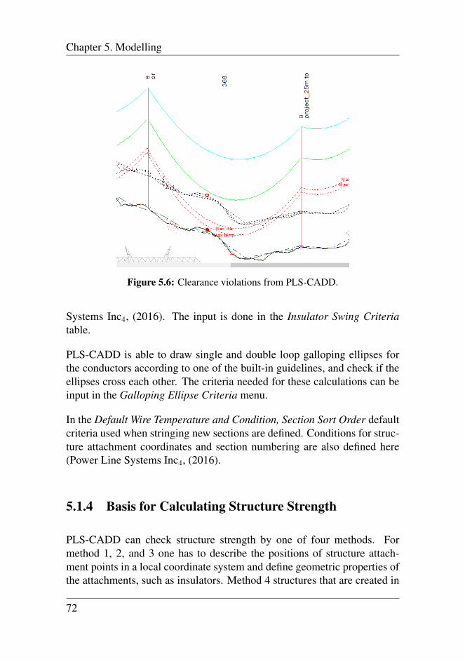
Chapter 5. Modelling
Figure 5.6: Clearance violations from PLS-CADD.
Systems Inc4, (2016). The input is done in the Insulator Swing Criteriatable.
PLS-CADD is able to draw single and double loop galloping ellipses forthe conductors according to one of the built-in guidelines, and check if theellipses cross each other. The criteria needed for these calculations can beinput in the Galloping Ellipse Criteria menu.
In the Default Wire Temperature and Condition, Section Sort Order defaultcriteria used when stringing new sections are defined. Conditions for struc-ture attachment coordinates and section numbering are also defined here(Power Line Systems Inc4, (2016).
5.1.4 Basis for Calculating Structure Strength
PLS-CADD can check structure strength by one of four methods. Formethod 1, 2, and 3 one has to describe the positions of structure attach-ment points in a local coordinate system and define geometric properties ofthe attachments, such as insulators. Method 4 structures that are created in
72

5.1 Modelling of Line in PLS-CADD
either PLS-TOWER or PLS-POLE has this data automatically included intheir structure files. The level of modelling will also influence the calcula-tions. For level 1 the ruling span is used and the horizontal tension compo-nent is assumed constant for all spans in one tension section (between twodead end towers), whereas for level 2, 3 and 4 the finite element methodis used so that each span can have different horizontal tension (Power LineSystems Inc4, (2016).
Method 1 for checking structure strength is based on actual and allowablewind and weight spans. The actual wind span, or horizontal span, at astructure is the average length of the cables on either side of the structure.The actual weight span, or vertical span, is the vertical distance betweenthe lowest points of the two adjacent spans. It is important to rememberthat the geometry of the cable can make the lowest point appear outsideof the span in question. As the geometry of the cables varies with whatload cases are applied, the weight span is calculated for three specifiedweather cases and cable conditions. Different cases are used to take intoaccount the fact that weight spans for conductors with ice are shorter thanwithout ice and thus need other allowed values. Common cases to checkfor include extreme wind, extreme cold and extreme ice. For each of thesecases allowable weight spans are calculated, in addition to the wind spanand minimum weight span so that no strength or serviceability violationsoccur for a range of line angles. Figure 5.7 illustrates this. If the calculatedvalues fall inside the marked areas, the strength of the structure is sufficient(Power Line Systems Inc4, (2016).
Figure 5.7: Method 1. Figure 8.3-1 of (Power Line Systems Inc4, (2016))
With method 2 interaction between separate spans are taken into account.
73
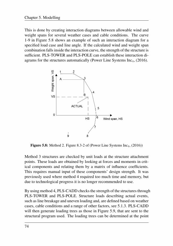
Chapter 5. Modelling
This is done by creating interaction diagrams between allowable wind andweight spans for several weather cases and cable conditions. The curve1-9 in Figure 5.8 shows an example of such an interaction diagram for aspecified load case and line angle. If the calculated wind and weight spancombination falls inside the interaction curve, the strength of the structure issufficient. PLS-TOWER and PLS-POLE can establish these interaction di-agrams for the structures automatically (Power Line Systems Inc4, (2016).
Figure 5.8: Method 2. Figure 8.3-2 of (Power Line Systems Inc4, (2016))
Method 3 structures are checked by unit loads at the structure attachmentpoints. These loads are obtained by looking at forces and moments in crit-ical components and relating them by a matrix of influence coefficients.This requires manual input of these components’ design strength. It waspreviously used where method 4 required too much time and memory, butdue to technological progress it is no longer recommended to use.
By using method 4, PLS-CADD checks the strength of the structures throughPLS-TOWER and PLS-POLE. Structure loads describing actual events,such as line breakage and uneven loading and, are defined based on weathercases, cable conditions and a range of other factors, see 5.1.3. PLS-CADDwill then generate loading trees as those in Figure 5.9, that are sent to thestructural program used. The loading trees can be determined at the point
74
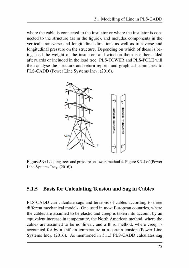
5.1 Modelling of Line in PLS-CADD
where the cable is connected to the insulator or where the insulator is con-nected to the structure (as in the figure), and includes components in thevertical, transverse and longitudinal directions as well as transverse andlongitudinal pressure on the structure. Depending on which of these is be-ing used the weight of the insulators and wind on them is either addedafterwards or included in the load tree. PLS-TOWER and PLS-POLE willthen analyse the structure and return reports and graphical summaries toPLS-CADD (Power Line Systems Inc4, (2016).
Figure 5.9: Loading trees and pressure on tower, method 4. Figure 8.3-4 of (PowerLine Systems Inc4, (2016))
5.1.5 Basis for Calculating Tension and Sag in Cables
PLS-CADD can calculate sags and tensions of cables according to threedifferent mechanical models. One used in most European countries, wherethe cables are assumed to be elastic and creep is taken into account by anequivalent increase in temperature, the North American method, where thecables are assumed to be nonlinear, and a third method, where creep isaccounted for by a shift in temperature at a certain tension (Power LineSystems Inc4, (2016). As mentioned in 5.1.3 PLS-CADD calculates sag
75
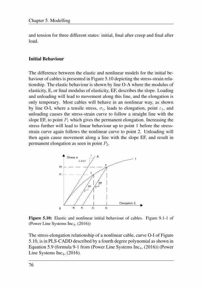
Chapter 5. Modelling
and tension for three different states: initial, final after creep and final afterload.
Initial Behaviour
The difference between the elastic and nonlinear models for the initial be-haviour of cables is presented in Figure 5.10 depicting the stress-strain rela-tionship. The elastic behaviour is shown by line O-A where the modulus ofelasticity, E, or final modulus of elasticity, EF, describes the slope. Loadingand unloading will lead to movement along this line, and the elongation isonly temporary. Most cables will behave in an nonlinear way, as shownby line O-I, where a tensile stress, σ1, leads to elongation, point ε1, andunloading causes the stress-strain curve to follow a straight line with theslope EF, to point P1 which gives the permanent elongation. Increasing thestress further will lead to linear behaviour up to point 1 before the stress-strain curve again follows the nonlinear curve to point 2. Unloading willthen again cause movement along a line with the slope EF, and result inpermanent elongation as seen in point P2.
Figure 5.10: Elastic and nonlinear initial behaviour of cables. Figure 9.1-1 of(Power Line Systems Inc4, (2016))
The stress-elongation relationship of a nonlinear cable, curve O-I of Figure5.10, is in PLS-CADD described by a fourth degree polynomial as shown inEquation 5.9 (formula 9-1 from (Power Line Systems Inc4, (2016)) (PowerLine Systems Inc4, (2016).
76
5.1 Modelling of Line in PLS-CADD
σ = k0 + k1 ∗ ε+ k2 ∗ ε2 + k3 ∗ ε3 + k4 ∗ ε4 (5.9)
Where:σ = tensile stress in cablek0,1,2,3,4 = coefficients found by curve fitting of experimental dataε = elongation expressed in percent of the cable reference
unstressed length
By setting k0, k2, k3 and k4 equal to zero and k1 equal to E, Equation 5.9can be used for a linear elastic cable as well (Power Line Systems Inc4,(2016).
When using composite cables, such as ACSR- (used in this thesis), ACAR-or SSAC-conductors, the stress-strain curve is obtained by combining thetwo materials’ stress-strain curves. This is illustrated in Figure 5.11. Equa-tion 5.10 (formula 9-2 from (Power Line Systems Inc4, (2016)) shows howto combine the two curves. The stresses in the outer and core materialscan be found using Equation 5.9, where the coefficients model the stressadjusted by the ratio of that material’s area to the total cable area as inEquation 5.11 and 5.12 (Power Line Systems Inc4, (2016).
σ = σO ∗ (ARO
AT) + σC ∗ (
ARC
AT) (5.10)
σO ∗ (ARO
AT) = a0 + a1 ∗ ε+ a2 ∗ ε2 + a3 ∗ ε3 + a4 ∗ ε4 (5.11)
σC ∗ (ARC
AT) = b0 + b1 ∗ ε+ b2 ∗ ε2 + b3 ∗ ε3 + b4 ∗ ε4 (5.12)
Where:σ = combined tensile stress in cableσO = stress in outer materialσC = stress in core materialARO = area of outer materialARC = area of core materialAT = ARO + ARC (total cable area)a0,1,2,3,4 = coefficients for outer material adjusted accordinglyb0,1,2,3,4 = coefficients for core material adjusted accordingly
77
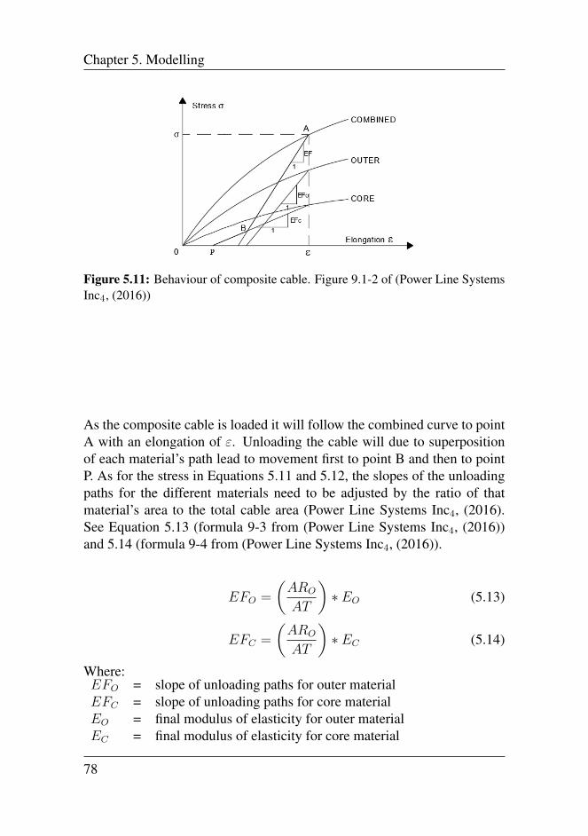
Chapter 5. Modelling
Figure 5.11: Behaviour of composite cable. Figure 9.1-2 of (Power Line SystemsInc4, (2016))
As the composite cable is loaded it will follow the combined curve to pointA with an elongation of ε. Unloading the cable will due to superpositionof each material’s path lead to movement first to point B and then to pointP. As for the stress in Equations 5.11 and 5.12, the slopes of the unloadingpaths for the different materials need to be adjusted by the ratio of thatmaterial’s area to the total cable area (Power Line Systems Inc4, (2016).See Equation 5.13 (formula 9-3 from (Power Line Systems Inc4, (2016))and 5.14 (formula 9-4 from (Power Line Systems Inc4, (2016)).
EFO =
(ARO
AT
)∗ EO (5.13)
EFC =
(ARO
AT
)∗ EC (5.14)
Where:EFO = slope of unloading paths for outer materialEFC = slope of unloading paths for core materialEO = final modulus of elasticity for outer materialEC = final modulus of elasticity for core material
78
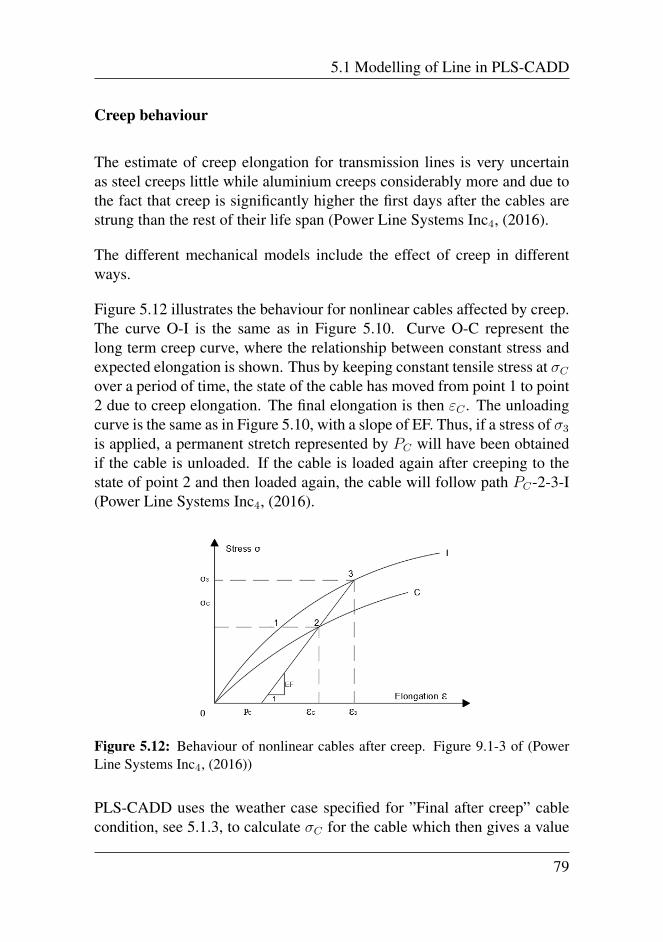
5.1 Modelling of Line in PLS-CADD
Creep behaviour
The estimate of creep elongation for transmission lines is very uncertainas steel creeps little while aluminium creeps considerably more and due tothe fact that creep is significantly higher the first days after the cables arestrung than the rest of their life span (Power Line Systems Inc4, (2016).
The different mechanical models include the effect of creep in differentways.
Figure 5.12 illustrates the behaviour for nonlinear cables affected by creep.The curve O-I is the same as in Figure 5.10. Curve O-C represent thelong term creep curve, where the relationship between constant stress andexpected elongation is shown. Thus by keeping constant tensile stress at σCover a period of time, the state of the cable has moved from point 1 to point2 due to creep elongation. The final elongation is then εC . The unloadingcurve is the same as in Figure 5.10, with a slope of EF. Thus, if a stress of σ3is applied, a permanent stretch represented by PC will have been obtainedif the cable is unloaded. If the cable is loaded again after creeping to thestate of point 2 and then loaded again, the cable will follow path PC-2-3-I(Power Line Systems Inc4, (2016).
Figure 5.12: Behaviour of nonlinear cables after creep. Figure 9.1-3 of (PowerLine Systems Inc4, (2016))
PLS-CADD uses the weather case specified for ”Final after creep” cablecondition, see 5.1.3, to calculate σC for the cable which then gives a value
79
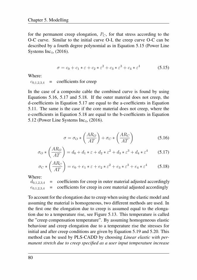
Chapter 5. Modelling
for the permanent creep elongation, PC , for that stress according to theO-C curve. Similar to the initial curve O-I, the creep curve O-C can bedescribed by a fourth degree polynomial as in Equation 5.15 (Power LineSystems Inc4, (2016).
σ = c0 + c1 ∗ ε+ c2 ∗ ε2 + c3 ∗ ε3 + c4 ∗ ε4 (5.15)
Where:c0,1,2,3,4 = coefficients for creep
In the case of a composite cable the combined curve is found by usingEquations 5.16, 5.17 and 5.18. If the outer material does not creep, thed-coefficients in Equation 5.17 are equal to the a-coefficients in Equation5.11. The same is the case if the core material does not creep, where thee-coefficients in Equation 5.18 are equal to the b-coefficients in Equation5.12 (Power Line Systems Inc4, (2016).
σ = σO ∗(ARO
AT
)+ σC ∗
(ARC
AT
)(5.16)
σO ∗(ARO
AT
)= d0 + d1 ∗ ε+ d2 ∗ ε2 + d3 ∗ ε3 + d4 ∗ ε4 (5.17)
σC ∗(ARC
AT
)= e0 + e1 ∗ ε+ e2 ∗ ε2 + e3 ∗ ε3 + e4 ∗ ε4 (5.18)
Where:d0,1,2,3,4 = coefficients for creep in outer material adjusted accordinglye0,1,2,3,4 = coefficients for creep in core material adjusted accordingly
To account for the elongation due to creep when using the elastic model andassuming the material is homogeneous, two different methods are used. Inthe first one the elongation due to creep is assumed equal to the elonga-tion due to a temperature rise, see Figure 5.13. This temperature is calledthe ”creep compensation temperature”. By assuming homogeneous elasticbehaviour and creep elongation due to a temperature rise the stresses forinitial and after creep conditions are given by Equation 5.19 and 5.20. Thismethod can be used by PLS-CADD by choosing Linear elastic with per-manent stretch due to creep specified as a user input temperature increase
80
5.1 Modelling of Line in PLS-CADD
in the cable data file (Power Line Systems Inc4, (2016).
Figure 5.13: Elastic cable with creep due to temperature rise. Figure 9.1-3a of(Power Line Systems Inc4, (2016))
σ = E ∗ ε (5.19)
σ = −E ∗ PC + E ∗ ε = −E ∗ αt+ E ∗ ε (5.20)
Where:E = elastic modulusε = elongation expressed in percent of the cable reference unstressed
lengthPC = creep elongation due to temperature riseα = thermal expansion coefficient for cablet = temperature shift used to model long term creep
The second method assumes that the creep varies proportionally with ten-sion as illustrated in Figure 5.14. Thus the initial stress is still calculated byEquation 5.19, while after creep the stress can be calculated by Equation5.21. This method can be used by PLS-CADD by choosing Linear elasticwith permanent stretch due to creep proportional to tension in the cabledata file (Power Line Systems Inc4, (2016).
81
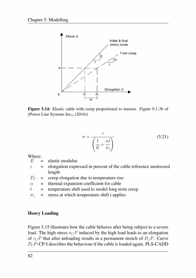
Chapter 5. Modelling
Figure 5.14: Elastic cable with creep proportional to tension. Figure 9.1-3b of(Power Line Systems Inc4, (2016))
σ =ε(
1
E+αt
σ1
) (5.21)
Where:E = elastic modulusε = elongation expressed in percent of the cable reference unstressed
lengthPC = creep elongation due to temperature riseα = thermal expansion coefficient for cablet = temperature shift used to model long term creepσ1 = stress at which temperature shift t applies
Heavy Loading
Figure 5.15 illustrates how the cable behaves after being subject to a severeload. The high stress σCP induced by the high load leads to an elongationof εCP that after unloading results in a permanent stretch of PCP . CurvePCP -CP-I describes the behaviour if the cable is loaded again. PLS-CADD
82
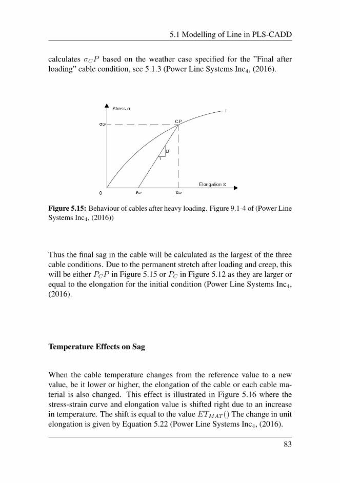
5.1 Modelling of Line in PLS-CADD
calculates σCP based on the weather case specified for the ”Final afterloading” cable condition, see 5.1.3 (Power Line Systems Inc4, (2016).
Figure 5.15: Behaviour of cables after heavy loading. Figure 9.1-4 of (Power LineSystems Inc4, (2016))
Thus the final sag in the cable will be calculated as the largest of the threecable conditions. Due to the permanent stretch after loading and creep, thiswill be either PCP in Figure 5.15 or PC in Figure 5.12 as they are larger orequal to the elongation for the initial condition (Power Line Systems Inc4,(2016).
Temperature Effects on Sag
When the cable temperature changes from the reference value to a newvalue, be it lower or higher, the elongation of the cable or each cable ma-terial is also changed. This effect is illustrated in Figure 5.16 where thestress-strain curve and elongation value is shifted right due to an increasein temperature. The shift is equal to the value ETMAT () The change in unitelongation is given by Equation 5.22 (Power Line Systems Inc4, (2016).
83

Chapter 5. Modelling
Figure 5.16: Effect of change in temperature. Figure 9.1-5 of (Power Line Sys-tems Inc4, (2016))
(∆L
LREF
)MAT
= ETMAT (TEMP − TEMPREF ) (5.22)
Where:∆L = change in lengthLREF = unstressed cable reference lengthETMAT = thermal expansion coefficient of material MATTEMP = new temperatureTEMPREF = reference temperature
5.1.6 Reports
In the Lines menu, PLS-CADD offers a range of checks and reports. Thestructure usage report provides structure strength usage, insulator swingusage, joint support reactions, loads at insulator attachments and anglemember checks (for latticed tower). The sections usage report gives thetension forces in all spans. PLS-CADD can make reports on survey pointclearances, clearance to TIN, danger tree locator, structure clearances andwire clearances.
84
5.1 Modelling of Line in PLS-CADD
5.1.7 Structure and Section Modelling
In the Structures menu, structures can be added, edited, moved or deleted.If the structures are modelled already, for example in PLS-TOWER or PLS-POLE, these structures can be used or edited. If not, then this menu alsooffers the possibility of creating new structures, like stick figures. They canbe either dead end structures or not, of a specified height, with specifiedsets and phases, all with a chosen insulator type, see Figure D.13.
As for the structures, PLS-CADD offers options for adding, editing anddeleting cables. This is done in the Sections menu. It is also possible toedit existing cable files or create new ones, as well as checking the sag andtension of the different cables.
Minimum two dead end towers need to be placed along the alignment be-fore a wire can be strung. It is less work to string the wire before addingintermediate structures, but it does not have to be done in this order. Whenmodelling this line, dead end stick figures of 18m height were created andplaced approximately 4.5km apart along the alignment. The input for thesestructures can be seen in Figure D.12. Three triplex Grackle conductors,see Figure D.5, were then strung between the dead end towers from phases1:1, 2:1 and 3:1 to 11:1, 22:1 and 33:1 respectively, 1 and 11 being on oneside and 3 and 33 on the other. It is important to make sure the conductorsare strung correctly so that they do not cross. This can easily be checked inthe plan view or 3D-view. Two ground wires, of the type F 69 Sveid, seeFigure D.7, were also strung, from phases 4:1 to 4:1 and 5:1 to 5:1.
The initial tension of the conductors was set to 39651N and the initial ten-sion of the ground wires was calculated to 25050N so that the sag of theground wires would not exceed that of the conductors, thus maintaining therequired clearance between them. See Appendix C.4 for this calculation.
Then the tower spotting of the intermediate structures was done. Thirteentowers were added at approximately 350m intervals and adjusted to main-tain the clearances specified in 5.1.3. Three separate PLS-CADD modelswere made; one with lattice towers, one with tubular steel and the last usingFRP structures. To simplify the production and erection processes and min-imize the costs it was decided to keep the structures to as similar heights as
85
Chapter 5. Modelling
possible when tower spotting.
Instead of doing the tower spotting manually, PLS-CADD is able to doautomatic tower spotting based on the criteria input and limitations likespotting constraints for prohibited and extra cost zones along the align-ment. This was not used in the model, but can be selected in the AutomaticSpotting menu.
An illustrating selection of input from PLS-CADD is shown in AppendixD.1.
5.2 Modelling in PLS-TOWER
5.2.1 Basis for Modelling
Like for PLS-CADD several standards can be used for the design checks.EN 50341-1 (CENELEC, (2012) is used here.
PLS-TOWER is organised so that the user can import component data basesor libraries for the different elements; such as steel angles, bolts, guys,insulators, cables and so on, in the Preferences menu. The elements canalso be defined manually under the Components menu if desired. Fromthe elements defined the model can be built in the Geometry menu. Fromthis model the computer will generate a finite element model (Power LineSystems Inc6, (2016).
The finite element model can either be linear or nonlinear. The linear modelignores P-∆ effects and models guys and cables as tension only members.The nonlinear model takes P-∆ effects into account, which enables PLS-TOWER to detect buckling and gives a better cable representation by mod-elling cables and guys as exact cable members. It is therefore recommendedto use the nonlinear model for finite analysis of guyed towers (Power LineSystems Inc6, (2016).
The analysis of the finite element model is done by PLS-TOWER using so-lution algorithms implemented in the program. Two modes are available:
86
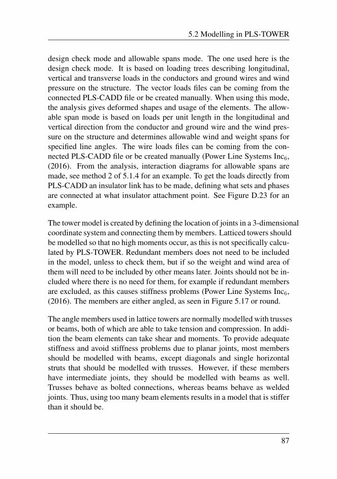
5.2 Modelling in PLS-TOWER
design check mode and allowable spans mode. The one used here is thedesign check mode. It is based on loading trees describing longitudinal,vertical and transverse loads in the conductors and ground wires and windpressure on the structure. The vector loads files can be coming from theconnected PLS-CADD file or be created manually. When using this mode,the analysis gives deformed shapes and usage of the elements. The allow-able span mode is based on loads per unit length in the longitudinal andvertical direction from the conductor and ground wire and the wind pres-sure on the structure and determines allowable wind and weight spans forspecified line angles. The wire loads files can be coming from the con-nected PLS-CADD file or be created manually (Power Line Systems Inc6,(2016). From the analysis, interaction diagrams for allowable spans aremade, see method 2 of 5.1.4 for an example. To get the loads directly fromPLS-CADD an insulator link has to be made, defining what sets and phasesare connected at what insulator attachment point. See Figure D.23 for anexample.
The tower model is created by defining the location of joints in a 3-dimensionalcoordinate system and connecting them by members. Latticed towers shouldbe modelled so that no high moments occur, as this is not specifically calcu-lated by PLS-TOWER. Redundant members does not need to be includedin the model, unless to check them, but if so the weight and wind area ofthem will need to be included by other means later. Joints should not be in-cluded where there is no need for them, for example if redundant membersare excluded, as this causes stiffness problems (Power Line Systems Inc6,(2016). The members are either angled, as seen in Figure 5.17 or round.
The angle members used in lattice towers are normally modelled with trussesor beams, both of which are able to take tension and compression. In addi-tion the beam elements can take shear and moments. To provide adequatestiffness and avoid stiffness problems due to planar joints, most membersshould be modelled with beams, except diagonals and single horizontalstruts that should be modelled with trusses. However, if these membershave intermediate joints, they should be modelled with beams as well.Trusses behave as bolted connections, whereas beams behave as weldedjoints. Thus, using too many beam elements results in a model that is stifferthan it should be.
87
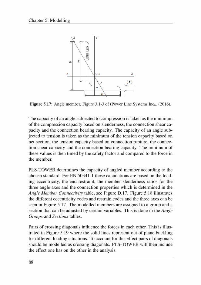
Chapter 5. Modelling
Figure 5.17: Angle member. Figure 3.1-3 of (Power Line Systems Inc6, (2016).
The capacity of an angle subjected to compression is taken as the minimumof the compression capacity based on slenderness, the connection shear ca-pacity and the connection bearing capacity. The capacity of an angle sub-jected to tension is taken as the minimum of the tension capacity based onnet section, the tension capacity based on connection rupture, the connec-tion shear capacity and the connection bearing capacity. The minimum ofthese values is then timed by the safety factor and compared to the force inthe member.
PLS-TOWER determines the capacity of angled member according to thechosen standard. For EN 50341-1 these calculations are based on the load-ing eccentricity, the end restraint, the member slenderness ratios for thethree angle axes and the connection properties which is determined in theAngle Member Connectivity table, see Figure D.17. Figure 5.18 illustratesthe different eccentricity codes and restrain codes and the three axes can beseen in Figure 5.17. The modelled members are assigned to a group and asection that can be adjusted by certain variables. This is done in the AngleGroups and Sections tables.
Pairs of crossing diagonals influence the forces in each other. This is illus-trated in Figure 5.19 where the solid lines represent out of plane bucklingfor different loading situations. To account for this effect pairs of diagonalsshould be modelled as crossing diagonals. PLS-TOWER will then includethe effect one has on the other in the analysis.
88
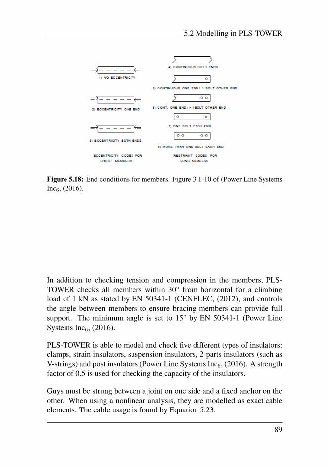
5.2 Modelling in PLS-TOWER
Figure 5.18: End conditions for members. Figure 3.1-10 of (Power Line SystemsInc6, (2016).
In addition to checking tension and compression in the members, PLS-TOWER checks all members within 30° from horizontal for a climbingload of 1 kN as stated by EN 50341-1 (CENELEC, (2012), and controlsthe angle between members to ensure bracing members can provide fullsupport. The minimum angle is set to 15° by EN 50341-1 (Power LineSystems Inc6, (2016).
PLS-TOWER is able to model and check five different types of insulators:clamps, strain insulators, suspension insulators, 2-parts insulators (such asV-strings) and post insulators (Power Line Systems Inc6, (2016). A strengthfactor of 0.5 is used for checking the capacity of the insulators.
Guys must be strung between a joint on one side and a fixed anchor on theother. When using a nonlinear analysis, they are modelled as exact cableelements. The cable usage is found by Equation 5.23.
89

Chapter 5. Modelling
Figure 5.19: Crossing diagonals. Figure 3.1-12 of (Power Line Systems Inc6,(2016)
Usage =T
TCAPxPCTx100xSF )(5.23)
Where:T = Tension force in cableTCAP = Tension capacity of cablePCT = Allowed percent of ultimate tensionSF = Safety factor
The loads affecting the tower are wire loads, dead loads and wind loadson the tower structure. Some standards also include ice load on members.The wire loads are the results of ice and wind loads on the conductors andground wires. The dead load is calculated automatically by PLS-TOWER(Power Line Systems Inc6, (2016).
As mentioned in 5.1.2 PLS-TOWER will use the input from PLS-CADD tocalculate the wind load on the structure. There are three models on how toapply wind loads on the structures: standard wind on face, standard wind onall and SAPS. The last one applies wind load to all members and assumesno shielding. It is thus a conservative model and is used here. Figure 5.20illustrates how the model works. A wind pressure is defined for a givenreference height. Above this the wind velocity increases with height (PowerLine Systems Inc6, (2016).
90
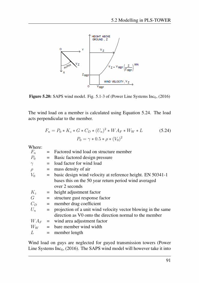
5.2 Modelling in PLS-TOWER
Figure 5.20: SAPS wind model. Fig. 5.1-3 of (Power Line Systems Inc6, (2016)
The wind load on a member is calculated using Equation 5.24. The loadacts perpendicular to the member.
Fn = P0 ∗Kz ∗G ∗ CD ∗ (Un)2 ∗WAF ∗WW ∗ L (5.24)
P0 = γ ∗ 0.5 ∗ ρ ∗ (V0)2
Where:Fn = Factored wind load on structure memberP0 = Basic factored design pressureγ = load factor for wind loadρ = mass density of airV0 = basic design wind velocity at reference height. EN 50341-1
bases this on the 50 year return period wind averagedover 2 seconds
Kz = height adjustment factorG = structure gust response factorCD = member drag coefficientUn = projection of a unit wind velocity vector blowing in the same
direction as V0 onto the direction normal to the memberWAF = wind area adjustment factorWW = bare member wind widthL = member length
Wind load on guys are neglected for guyed transmission towers (PowerLine Systems Inc6, (2016). The SAPS wind model will however take it into
91
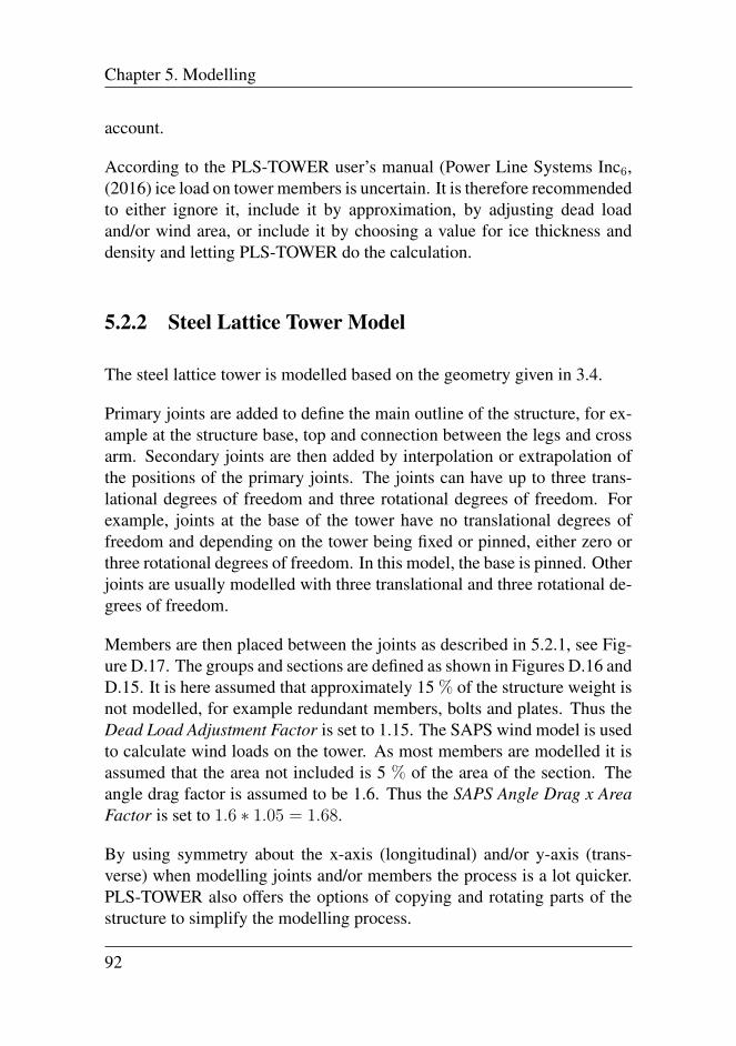
Chapter 5. Modelling
account.
According to the PLS-TOWER user’s manual (Power Line Systems Inc6,(2016) ice load on tower members is uncertain. It is therefore recommendedto either ignore it, include it by approximation, by adjusting dead loadand/or wind area, or include it by choosing a value for ice thickness anddensity and letting PLS-TOWER do the calculation.
5.2.2 Steel Lattice Tower Model
The steel lattice tower is modelled based on the geometry given in 3.4.
Primary joints are added to define the main outline of the structure, for ex-ample at the structure base, top and connection between the legs and crossarm. Secondary joints are then added by interpolation or extrapolation ofthe positions of the primary joints. The joints can have up to three trans-lational degrees of freedom and three rotational degrees of freedom. Forexample, joints at the base of the tower have no translational degrees offreedom and depending on the tower being fixed or pinned, either zero orthree rotational degrees of freedom. In this model, the base is pinned. Otherjoints are usually modelled with three translational and three rotational de-grees of freedom.
Members are then placed between the joints as described in 5.2.1, see Fig-ure D.17. The groups and sections are defined as shown in Figures D.16 andD.15. It is here assumed that approximately 15 % of the structure weight isnot modelled, for example redundant members, bolts and plates. Thus theDead Load Adjustment Factor is set to 1.15. The SAPS wind model is usedto calculate wind loads on the tower. As most members are modelled it isassumed that the area not included is 5 % of the area of the section. Theangle drag factor is assumed to be 1.6. Thus the SAPS Angle Drag x AreaFactor is set to 1.6 ∗ 1.05 = 1.68.
By using symmetry about the x-axis (longitudinal) and/or y-axis (trans-verse) when modelling joints and/or members the process is a lot quicker.PLS-TOWER also offers the options of copying and rotating parts of thestructure to simplify the modelling process.
92
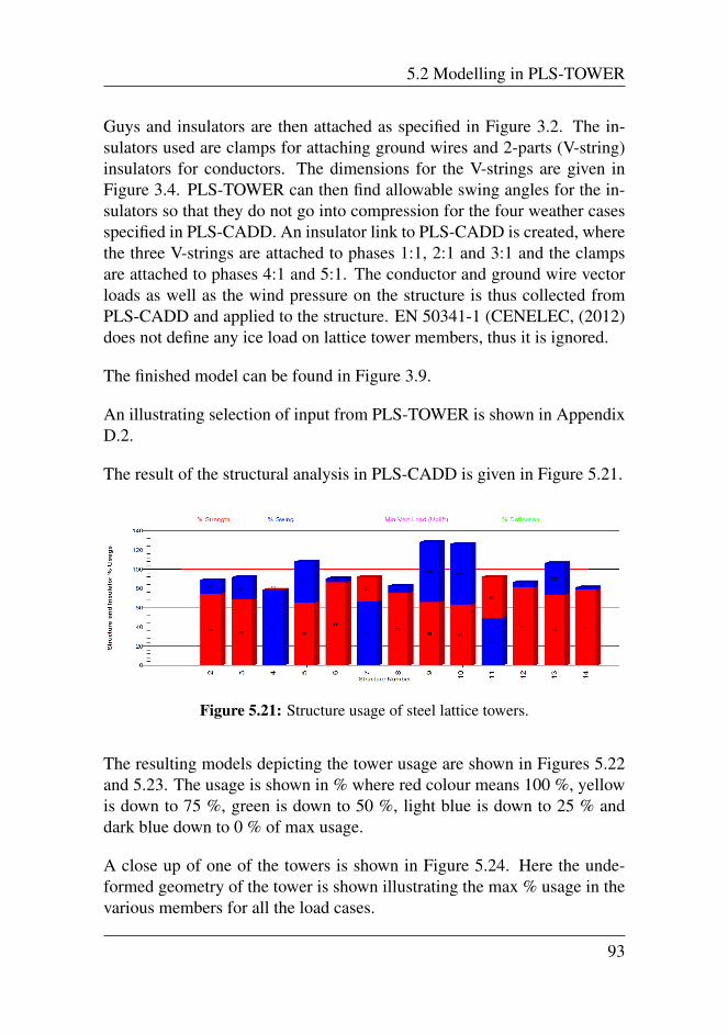
5.2 Modelling in PLS-TOWER
Guys and insulators are then attached as specified in Figure 3.2. The in-sulators used are clamps for attaching ground wires and 2-parts (V-string)insulators for conductors. The dimensions for the V-strings are given inFigure 3.4. PLS-TOWER can then find allowable swing angles for the in-sulators so that they do not go into compression for the four weather casesspecified in PLS-CADD. An insulator link to PLS-CADD is created, wherethe three V-strings are attached to phases 1:1, 2:1 and 3:1 and the clampsare attached to phases 4:1 and 5:1. The conductor and ground wire vectorloads as well as the wind pressure on the structure is thus collected fromPLS-CADD and applied to the structure. EN 50341-1 (CENELEC, (2012)does not define any ice load on lattice tower members, thus it is ignored.
The finished model can be found in Figure 3.9.
An illustrating selection of input from PLS-TOWER is shown in AppendixD.2.
The result of the structural analysis in PLS-CADD is given in Figure 5.21.
Figure 5.21: Structure usage of steel lattice towers.
The resulting models depicting the tower usage are shown in Figures 5.22and 5.23. The usage is shown in % where red colour means 100 %, yellowis down to 75 %, green is down to 50 %, light blue is down to 25 % anddark blue down to 0 % of max usage.
A close up of one of the towers is shown in Figure 5.24. Here the unde-formed geometry of the tower is shown illustrating the max % usage in thevarious members for all the load cases.
93
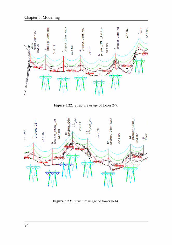
Chapter 5. Modelling
Figure 5.22: Structure usage of tower 2-7.
Figure 5.23: Structure usage of tower 8-14.
94
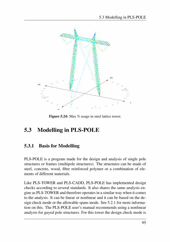
5.3 Modelling in PLS-POLE
Figure 5.24: Max % usage in steel lattice tower.
5.3 Modelling in PLS-POLE
5.3.1 Basis for Modelling
PLS-POLE is a program made for the design and analysis of single polestructures or frames (multipole structures). The structures can be made ofsteel, concrete, wood, fibre reinforced polymer or a combination of ele-ments of different materials.
Like PLS-TOWER and PLS-CADD, PLS-POLE has implemented designchecks according to several standards. It also shares the same analysis en-gine as PLS-TOWER and therefore operates in a similar way when it comesto the analysis. It can be linear or nonlinear and it can be based on the de-sign check mode or the allowable spans mode. See 5.2.1 for more informa-tion on this. The PLS-POLE user’s manual recommends using a nonlinearanalysis for guyed pole structures. For this tower the design check mode is
95
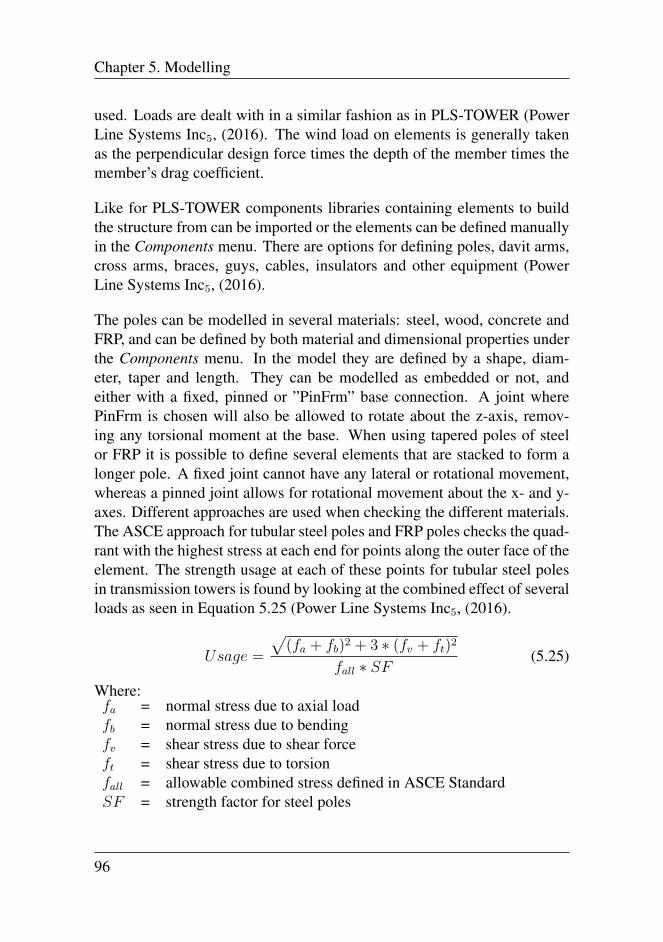
Chapter 5. Modelling
used. Loads are dealt with in a similar fashion as in PLS-TOWER (PowerLine Systems Inc5, (2016). The wind load on elements is generally takenas the perpendicular design force times the depth of the member times themember’s drag coefficient.
Like for PLS-TOWER components libraries containing elements to buildthe structure from can be imported or the elements can be defined manuallyin the Components menu. There are options for defining poles, davit arms,cross arms, braces, guys, cables, insulators and other equipment (PowerLine Systems Inc5, (2016).
The poles can be modelled in several materials: steel, wood, concrete andFRP, and can be defined by both material and dimensional properties underthe Components menu. In the model they are defined by a shape, diam-eter, taper and length. They can be modelled as embedded or not, andeither with a fixed, pinned or ”PinFrm” base connection. A joint wherePinFrm is chosen will also be allowed to rotate about the z-axis, remov-ing any torsional moment at the base. When using tapered poles of steelor FRP it is possible to define several elements that are stacked to form alonger pole. A fixed joint cannot have any lateral or rotational movement,whereas a pinned joint allows for rotational movement about the x- and y-axes. Different approaches are used when checking the different materials.The ASCE approach for tubular steel poles and FRP poles checks the quad-rant with the highest stress at each end for points along the outer face of theelement. The strength usage at each of these points for tubular steel polesin transmission towers is found by looking at the combined effect of severalloads as seen in Equation 5.25 (Power Line Systems Inc5, (2016).
Usage =
√(fa + fb)2 + 3 ∗ (fv + ft)2
fall ∗ SF(5.25)
Where:fa = normal stress due to axial loadfb = normal stress due to bendingfv = shear stress due to shear forceft = shear stress due to torsionfall = allowable combined stress defined in ASCE StandardSF = strength factor for steel poles
96
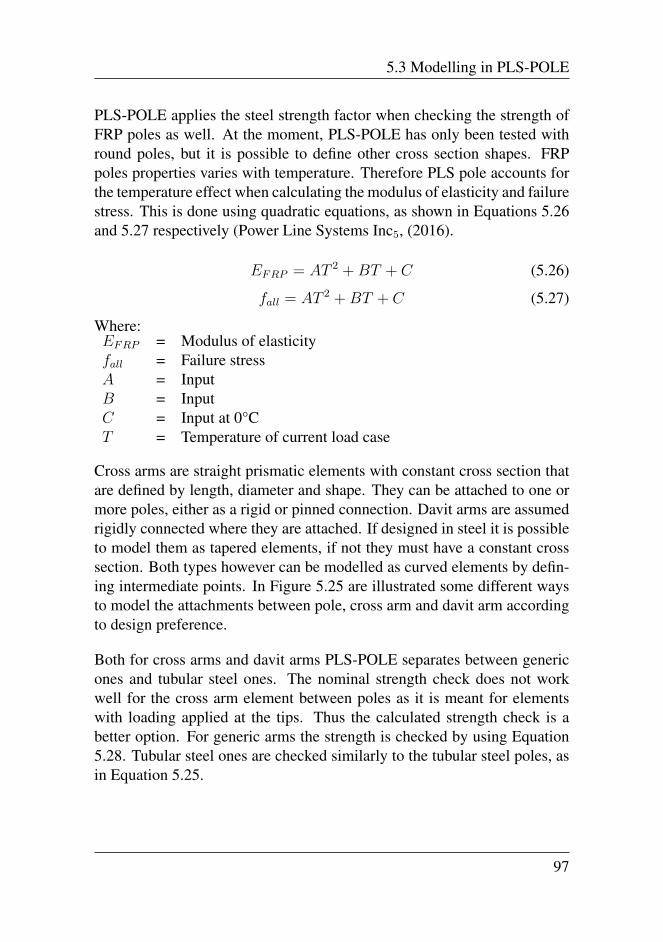
5.3 Modelling in PLS-POLE
PLS-POLE applies the steel strength factor when checking the strength ofFRP poles as well. At the moment, PLS-POLE has only been tested withround poles, but it is possible to define other cross section shapes. FRPpoles properties varies with temperature. Therefore PLS pole accounts forthe temperature effect when calculating the modulus of elasticity and failurestress. This is done using quadratic equations, as shown in Equations 5.26and 5.27 respectively (Power Line Systems Inc5, (2016).
EFRP = AT 2 +BT + C (5.26)
fall = AT 2 +BT + C (5.27)
Where:EFRP = Modulus of elasticityfall = Failure stressA = InputB = InputC = Input at 0°CT = Temperature of current load case
Cross arms are straight prismatic elements with constant cross section thatare defined by length, diameter and shape. They can be attached to one ormore poles, either as a rigid or pinned connection. Davit arms are assumedrigidly connected where they are attached. If designed in steel it is possibleto model them as tapered elements, if not they must have a constant crosssection. Both types however can be modelled as curved elements by defin-ing intermediate points. In Figure 5.25 are illustrated some different waysto model the attachments between pole, cross arm and davit arm accordingto design preference.
Both for cross arms and davit arms PLS-POLE separates between genericones and tubular steel ones. The nominal strength check does not workwell for the cross arm element between poles as it is meant for elementswith loading applied at the tips. Thus the calculated strength check is abetter option. For generic arms the strength is checked by using Equation5.28. Tubular steel ones are checked similarly to the tubular steel poles, asin Equation 5.25.
97
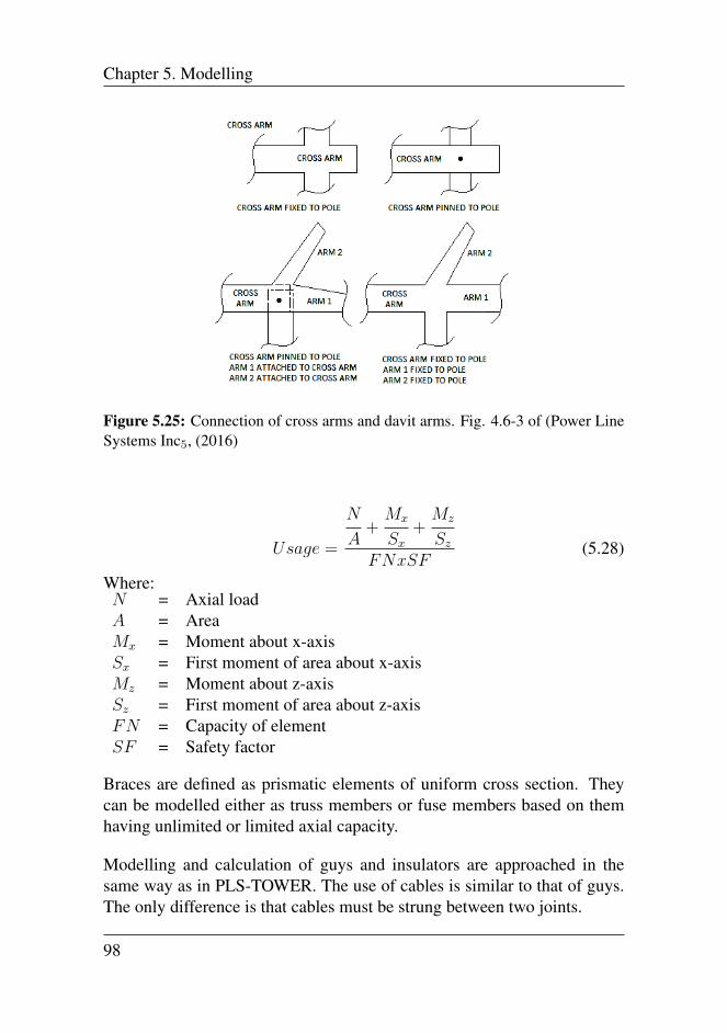
Chapter 5. Modelling
Figure 5.25: Connection of cross arms and davit arms. Fig. 4.6-3 of (Power LineSystems Inc5, (2016)
Usage =
N
A+Mx
Sx
+Mz
Sz
FNxSF(5.28)
Where:N = Axial loadA = AreaMx = Moment about x-axisSx = First moment of area about x-axisMz = Moment about z-axisSz = First moment of area about z-axisFN = Capacity of elementSF = Safety factor
Braces are defined as prismatic elements of uniform cross section. Theycan be modelled either as truss members or fuse members based on themhaving unlimited or limited axial capacity.
Modelling and calculation of guys and insulators are approached in thesame way as in PLS-TOWER. The use of cables is similar to that of guys.The only difference is that cables must be strung between two joints.
98
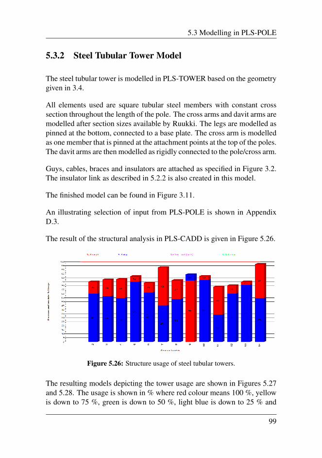
5.3 Modelling in PLS-POLE
5.3.2 Steel Tubular Tower Model
The steel tubular tower is modelled in PLS-TOWER based on the geometrygiven in 3.4.
All elements used are square tubular steel members with constant crosssection throughout the length of the pole. The cross arms and davit arms aremodelled after section sizes available by Ruukki. The legs are modelled aspinned at the bottom, connected to a base plate. The cross arm is modelledas one member that is pinned at the attachment points at the top of the poles.The davit arms are then modelled as rigidly connected to the pole/cross arm.
Guys, cables, braces and insulators are attached as specified in Figure 3.2.The insulator link as described in 5.2.2 is also created in this model.
The finished model can be found in Figure 3.11.
An illustrating selection of input from PLS-POLE is shown in AppendixD.3.
The result of the structural analysis in PLS-CADD is given in Figure 5.26.
Figure 5.26: Structure usage of steel tubular towers.
The resulting models depicting the tower usage are shown in Figures 5.27and 5.28. The usage is shown in % where red colour means 100 %, yellowis down to 75 %, green is down to 50 %, light blue is down to 25 % and
99
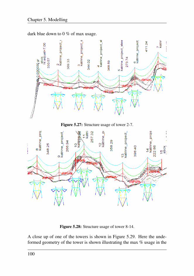
Chapter 5. Modelling
dark blue down to 0 % of max usage.
Figure 5.27: Structure usage of tower 2-7.
Figure 5.28: Structure usage of tower 8-14.
A close up of one of the towers is shown in Figure 5.29. Here the unde-formed geometry of the tower is shown illustrating the max % usage in the
100
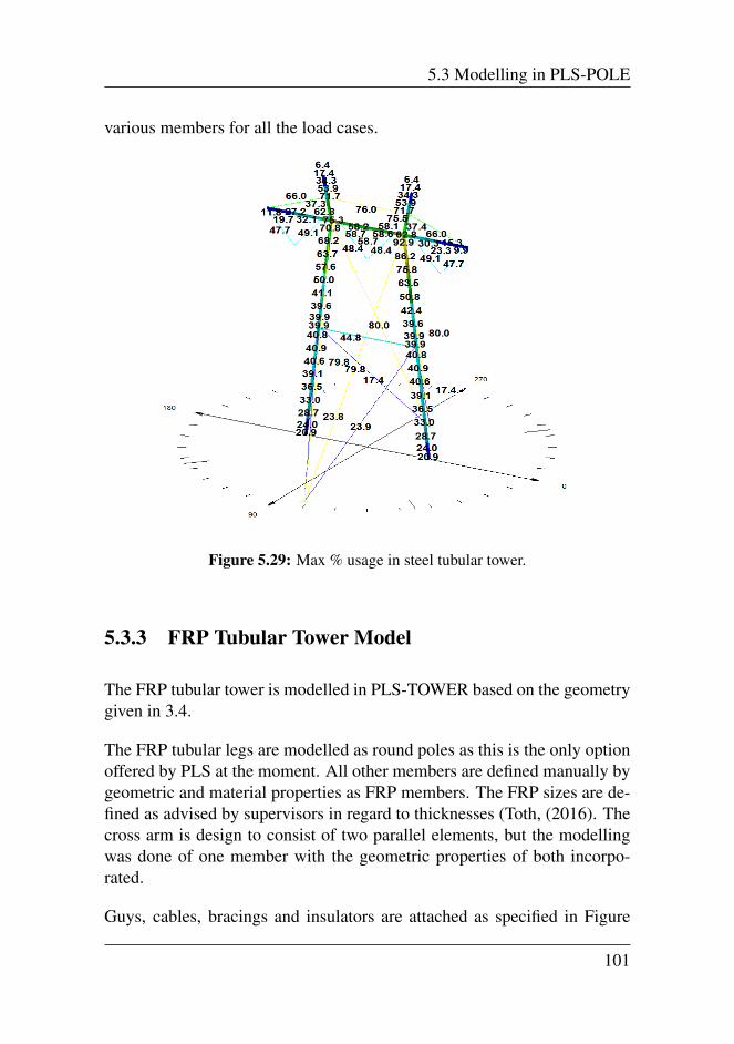
5.3 Modelling in PLS-POLE
various members for all the load cases.
Figure 5.29: Max % usage in steel tubular tower.
5.3.3 FRP Tubular Tower Model
The FRP tubular tower is modelled in PLS-TOWER based on the geometrygiven in 3.4.
The FRP tubular legs are modelled as round poles as this is the only optionoffered by PLS at the moment. All other members are defined manually bygeometric and material properties as FRP members. The FRP sizes are de-fined as advised by supervisors in regard to thicknesses (Toth, (2016). Thecross arm is design to consist of two parallel elements, but the modellingwas done of one member with the geometric properties of both incorpo-rated.
Guys, cables, bracings and insulators are attached as specified in Figure
101
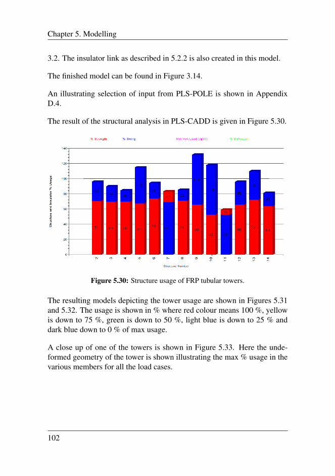
Chapter 5. Modelling
3.2. The insulator link as described in 5.2.2 is also created in this model.
The finished model can be found in Figure 3.14.
An illustrating selection of input from PLS-POLE is shown in AppendixD.4.
The result of the structural analysis in PLS-CADD is given in Figure 5.30.
Figure 5.30: Structure usage of FRP tubular towers.
The resulting models depicting the tower usage are shown in Figures 5.31and 5.32. The usage is shown in % where red colour means 100 %, yellowis down to 75 %, green is down to 50 %, light blue is down to 25 % anddark blue down to 0 % of max usage.
A close up of one of the towers is shown in Figure 5.33. Here the unde-formed geometry of the tower is shown illustrating the max % usage in thevarious members for all the load cases.
102
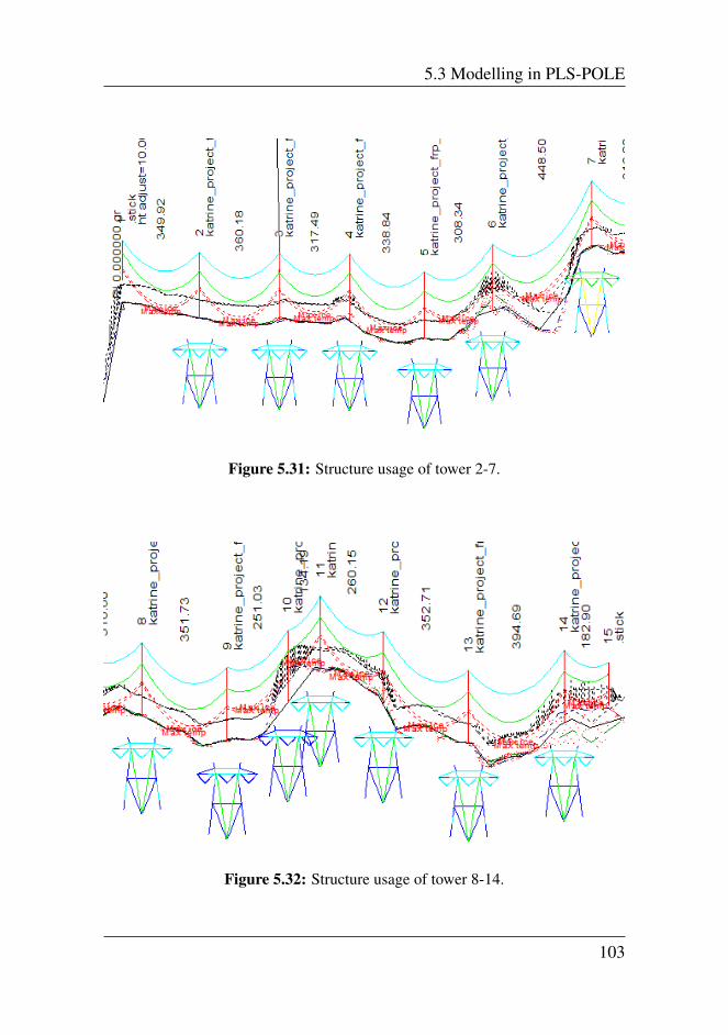
5.3 Modelling in PLS-POLE
Figure 5.31: Structure usage of tower 2-7.
Figure 5.32: Structure usage of tower 8-14.
103
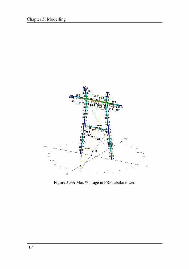
Chapter 5. Modelling
Figure 5.33: Max % usage in FRP tubular tower.
104
Chapter 6Calculations and Checks
6.1 Preliminary Calculations
The dead loads, wind loads and ice loads were applied to the structure lead-ing to forces in the vertical and transverse directions. From this, prelimi-nary cross sections were obtained.
The preliminary calculations are done based on assumptions that the rul-ing span is 350 m and that the towers are located on a straight line hori-zontally unless specified otherwise. It was in these calculations assumedthat the vertical components are taken as compression by the legs and thetransverse components to be taken as tension in the guys, yielding extracompression in the legs and crossarm. Also, for the tubular towers, onlythe guys connected to the cross arm were assumed to take any load.
6.1.1 Vertical loads
Vertical loads on the structures come from the dead load and the ice loadon conductors and ground wires. When assuming a weight span of 350m (assumes flat terrain) the vertical load on a support from ice load wasfound to be 52.5 kN for a conductor and 17.5 kN for a ground wire. See
105
Chapter 6. Calculations and Checks
Appendix C.2 for calculations. The dead load is the same as in 4.1, nowincluding conductors and ground wires.
Table 6.1: Vertical loads.
Tower Dead load (kN) Ice load (kN) Dead + Ice load (kN)Steel lattice tower 172.2 192.5 364.7Steel tubular tower 167.7 192.5 360.2FRP tubular tower 139.1 192.5 331.6
As mentioned, the vertical loads lead to compression forces in the legs andthe middle part of the cross arm. See Appendix C.5 for calculations. Theseforces are given in Table 6.2
Table 6.2: Forces due to vertical loads.
Tower Element Compressive force Compressive forceDue to dead load (kN) Due to dead + ice load (kN)
Steel lattice Leg 86.8 183.8Steel lattice Cross arm 10.8 22.8Steel tubular Leg 84.5 181.5Steel tubular Cross arm 10.5 22.5FRP tubular Leg 70.1 167.1FRP tubular Cross arm 8.7 20.7
6.1.2 Transverse loads
Wind on the cables lead to forces in attachment points of conductors andground wires. When applied parallel to the cross arm only two of the guyswill be in tension and take loads. The resulting forces will be divided intotension in the guys and compression in the legs. See Appendix B.1 forderivation of this.
In addition the wind load on the structure itself will affect the forces. Forsimplification all transverse loads are added at the top. The wind load cal-culated are presented in Table 4.4.
106
6.1 Preliminary Calculations
The forces in guys and legs found are presented in Table 6.3. See AppendixC.6 for calculations.
Table 6.3: Forces due to transverse loads.
Tower Element Force (kN)Steel lattice Leg 284Steel lattice Guy 158Steel tubular Leg 236Steel tubular Guy 131FRP tubular Leg 250FRP tubular Guy 139
6.1.3 Longitudinal loads
Ice load and wind load on the conductors and ground wires lead to in-creased tension in the cables. These loads will be taken by tension towersthroughout the line and the dead-end towers at each end. For suspensiontowers the longitudinal loads from the adjacent spans will more or less can-cel each other out if the spans and heights are of similar size. This will ofcourse rarely happen in real life, but for the simplicity of the preliminarycalculations, it is assumed that they do. Only when stringing the cables andat conductor breaks will these towers experience any longitudinal loading.
When loaded in the longitudinal direction, tension forces are taken by theguys resulting in compressive forces in the leg and cross arm. Derivationof the forces affecting the towers can be found in Appendix B.2.
6.1.4 Combined Forces
The combined forces from vertical, transverse and longitudinal loads aregiven in Table 6.4
107
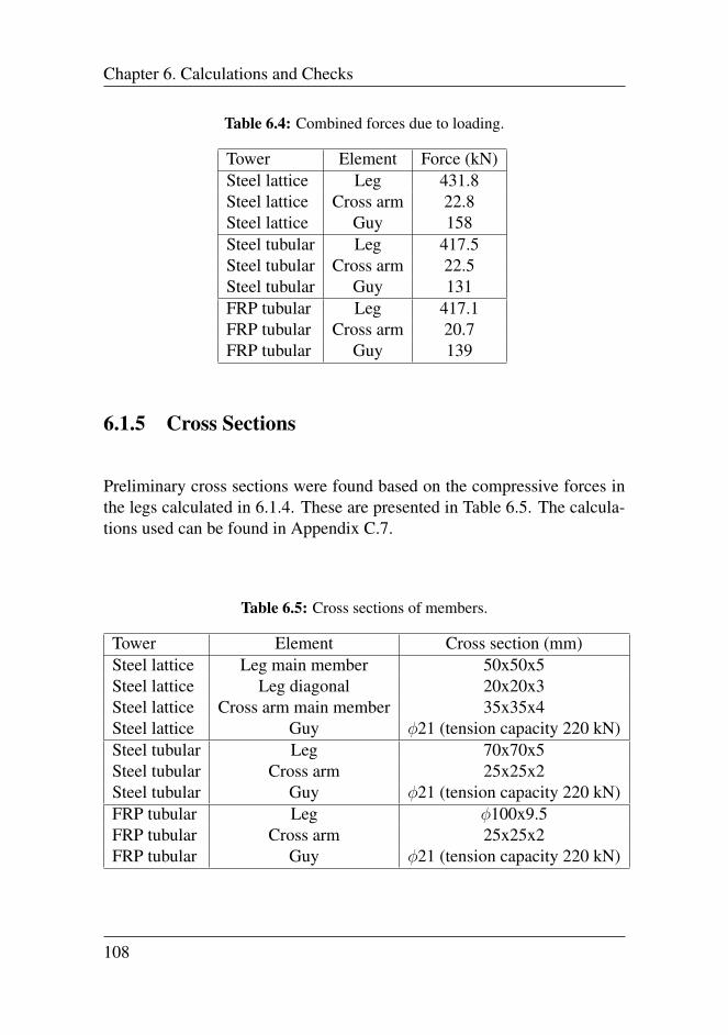
Chapter 6. Calculations and Checks
Table 6.4: Combined forces due to loading.
Tower Element Force (kN)Steel lattice Leg 431.8Steel lattice Cross arm 22.8Steel lattice Guy 158Steel tubular Leg 417.5Steel tubular Cross arm 22.5Steel tubular Guy 131FRP tubular Leg 417.1FRP tubular Cross arm 20.7FRP tubular Guy 139
6.1.5 Cross Sections
Preliminary cross sections were found based on the compressive forces inthe legs calculated in 6.1.4. These are presented in Table 6.5. The calcula-tions used can be found in Appendix C.7.
Table 6.5: Cross sections of members.
Tower Element Cross section (mm)Steel lattice Leg main member 50x50x5Steel lattice Leg diagonal 20x20x3Steel lattice Cross arm main member 35x35x4Steel lattice Guy φ21 (tension capacity 220 kN)Steel tubular Leg 70x70x5Steel tubular Cross arm 25x25x2Steel tubular Guy φ21 (tension capacity 220 kN)FRP tubular Leg φ100x9.5FRP tubular Cross arm 25x25x2FRP tubular Guy φ21 (tension capacity 220 kN)
108
6.2 PLS-checks
6.2 PLS-checks
6.2.1 Load calculation
Load case 10: wind on clear line (wind 500 year) on a conductor yields atransverse load applied to the structure of 30119 N in PLS. The calculatedtransverse wind load on a structure is 23909 N. This is not exactly the same,but may be a result of the wind model chosen in PLS. One can assume thatthe input is being correctly processed.
Load case 01: full ice load on a conductor yields a vertical load applied tothe structure of 52630 N in PLS. The calculated ice load for a weight spanof 350 m is 52500 N which is almost similar.
6.2.2 Deflections
The stiffness of a structure can be more critical than the strength, as a struc-ture that is too flexible might not be able to do its intended task of support-ing the hardware (Vinson and Sierakowski, (2012)). This might lead to linefailure.
The maximum deflection of a composite utility tower structure is 12 %of the height according to REN (Ren Elektrisk Nettvirksomhet AS). Thisequals a deflection at the top of 3.6 m, and for the cross arm ends 1.1 m.This requirement is checked against deflections for the tower top and crossarm acquired from PLS for all load cases. Both are within the requirement.
Maximum deflection of a steel utility tower structure is for suspension poles4 % of the pole length (Kiessling et al., (2003)). This equals a deflectionat the top of 1.2 m, and for the cross arm ends 0.3 m. This requirement ischecked against deflections for the tower top and cross arm acquired fromPLS for all load cases. Both are within the requirement.
For both towers the load cases yielding the largest deflections are in thetransverse direction 500 year wind on clear line and in the longitudinal
109
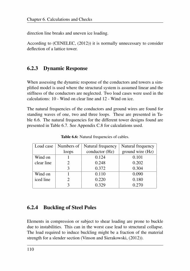
Chapter 6. Calculations and Checks
direction line breaks and uneven ice loading.
According to (CENELEC, (2012)) it is normally unnecessary to considerdeflection of a lattice tower.
6.2.3 Dynamic Response
When assessing the dynamic response of the conductors and towers a sim-plified model is used where the structural system is assumed linear and thestiffness of the conductors are neglected. Two load cases were used in thecalculations: 10 - Wind on clear line and 12 - Wind on ice.
The natural frequencies of the conductors and ground wires are found forstanding waves of one, two and three loops. These are presented in Ta-ble 6.6. The natural frequencies for the different tower designs found arepresented in Table 6.7. See Appendix C.8 for calculations used.
Table 6.6: Natural frequencies of cables.
Load case Numbers of Natural frequency Natural frequencyloops conductor (Hz) ground wire (Hz)
Wind on 1 0.124 0.101clear line 2 0.248 0.202
3 0.372 0.304Wind on 1 0.110 0.090iced line 2 0.220 0.180
3 0.329 0.270
6.2.4 Buckling of Steel Poles
Elements in compression or subject to shear loading are prone to buckledue to instabilities. This can in the worst case lead to structural collapse.The load required to induce buckling might be a fraction of the materialstrength for a slender section (Vinson and Sierakowski, (2012)).
110

6.2 PLS-checks
Table 6.7: Natural frequencies of towers.
Load case Tower Natural frequency (Hz)Wind on Steel lattice 0.651clear line Steel tubular 0.552
FRP tubular 0.472Wind on Steel lattice 1.009iced line Steel tubular 0.575
FRP tubular 0.525
Based on the moment distributions in the longitudinal and transverse direc-tions and the axial compression load, the buckling is checked according toNS-EN 1993-1-1:2005 (CEN, (2005)) by Clause 6.3.3 and Annex B. Loadcases 01: Full ice load and 10: 500 year wind on clear line were found toinduce the largest moments and axial loads and were thus the ones checked.It is assumed that the guys provide lateral stability, making the length of theelements 12.1 m.
The steel poles analysed do not buckle. See calculations in Appendix C.9.
111


Chapter 7Life Cycle Analyses
Life cycle analyses are done to evaluate a product based on all of its lifephases by summarising potential benefits and costs throughout its life span.Results of such analyses can be used for example to compare different de-signs or material usages, as is done here.
Both monetary cost and environmental impact is evaluated in this thesis.
These analyses are performed to give an additional basis for comparing thethree different designs defined in Chapter 3. All the towers are assumed tohave fairly similar foundations and equal insulators, conductors and groundwires. Thus the difference will mainly lie in the design of the tower itself.
For both the life cycle cost analysis and the environmental assessment thelife span of the tower is divided into several phases to describe the lifefrom raw material to decommissioning. The production phase is thought toinclude raw materials, transport of raw materials and manufacturing of ele-ments. The assembly phase consists of transport of finished elements eitherby ship, truck or both, and the assembly of the structure on site. The usephase is determined as the time span from when the tower is commissioneduntil it is taken out of service, thus including checks, any maintenance re-quired and possible repairs. The end-of-life phase consists of deconstruc-tion, transport, waste processing and disposal. Any recycling potential thematerials have will also be added here.
113
Chapter 7. Life Cycle Analyses
7.1 Theory
7.1.1 Life Cycle Cost
Life cycle cost (LCC), also called life cycle cost analysis (LCCA), takesinto account all costs of a product during its life span by discounting themto their present value to give a holistic look of the system (Wubbenhorst,(1986)). This is done with a goal of optimising value for money to resultin a cost efficient solution (Woodward, (1997)). By considering the costsof all life phases of the product it is easier to assess where in a project cutsin costs can be made. This is particularly important in a society where costoften is the most important aspect. LCC also offers a way to compare alter-natives based on both CapEx (Capital Expenditure) and OpEx (OperationalExpenditure).
An LCCA can be done in many ways. A general way is to first determinethe cost elements, then define the cost structure, for so to establish the costestimating relationship and finally establishing the method of LCC formu-lation. Other approaches might divide these phases further, like Kaufman’sformulation as mentioned by Woodward ((1997)). This divides the processinto eight steps.
On of the aspects to influence the LCC most is the discount rate used toget present values. A high discount rate favours options where the capitalcost is low and the life span short. A low one will then do the opposite(Woodward, (1997)). If this is not assessed correctly the LCC may wronglyfavour one alternative if costs and life span differ greatly. This can thus be aproblem when trying to show long term investments as more desirable thanshort term ones. The discount rate will be influenced by the inflation rateand base rate (Woodward, (1997)). The discount rate is set to 5% in thisthesis based on recommendations from supervisors.
A common tool for cost estimating is the net present value (NPV) method.By moving all future cash flows to the present, this tool enables us to eval-uate costs happening at different times in the future at a common principallevel by determining their present value. This is based on the interest rate,or discount rate (Remer and Nieto, (1995)). The net present value can be
114
7.1 Theory
found using Equation 7.1.
NPV =Ct
(1 + r)t(7.1)
Where:NPV = net present valueCt = cost in year tr = discount ratet = year
7.1.2 Life Cycle Assessment
In later years we as a society have begun to understand the importance ofpreserving our planet. The effects on the environment has greater impact onthe choices we make and the environmental impact has become a key factorwhen evaluating projects and choosing alternatives also in the constructionindustry (Alfredsen et al., (2012)).
The purpose of the life cycle assessment (LCA), also called environmentallife cycle assessment, is to evaluate the effect a product has on the environ-ment throughout its life span (The Environmental Literacy Council, (2015))and to find ways to reduce these effects while still maintaining its function-ality and quality. Some products might be composed of many elements thatwill all need to be taken into account to get a correct look at the problem.
To ensure the environmental aspect of a problem is given the correct amountof consideration and is used in a correct way the LCA should be conductedaccording to international guidelines given by ISO 14040: Environmentalmanagement - Life cycle assessment - Principles and framework (Alfredsenet al., (2012)).
ISO 14040 states that an LCA should be conducted in four phases: def-inition of goal and scope, inventory analysis, impact assessment and in-terpretation. Figure 7.1 illustrates how these phases influence each other(Alfredsen et al., (2012)).
115
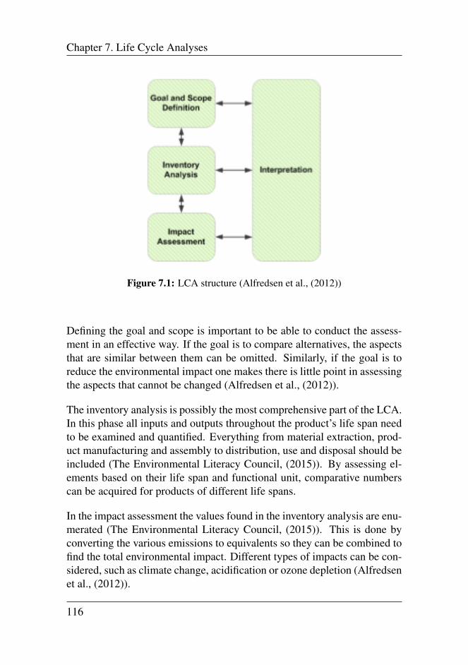
Chapter 7. Life Cycle Analyses
Figure 7.1: LCA structure (Alfredsen et al., (2012))
Defining the goal and scope is important to be able to conduct the assess-ment in an effective way. If the goal is to compare alternatives, the aspectsthat are similar between them can be omitted. Similarly, if the goal is toreduce the environmental impact one makes there is little point in assessingthe aspects that cannot be changed (Alfredsen et al., (2012)).
The inventory analysis is possibly the most comprehensive part of the LCA.In this phase all inputs and outputs throughout the product’s life span needto be examined and quantified. Everything from material extraction, prod-uct manufacturing and assembly to distribution, use and disposal should beincluded (The Environmental Literacy Council, (2015)). By assessing el-ements based on their life span and functional unit, comparative numberscan be acquired for products of different life spans.
In the impact assessment the values found in the inventory analysis are enu-merated (The Environmental Literacy Council, (2015)). This is done byconverting the various emissions to equivalents so they can be combined tofind the total environmental impact. Different types of impacts can be con-sidered, such as climate change, acidification or ozone depletion (Alfredsenet al., (2012)).
116
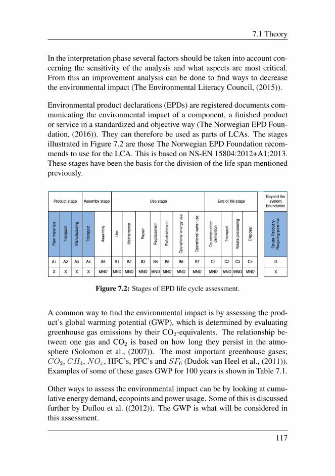
7.1 Theory
In the interpretation phase several factors should be taken into account con-cerning the sensitivity of the analysis and what aspects are most critical.From this an improvement analysis can be done to find ways to decreasethe environmental impact (The Environmental Literacy Council, (2015)).
Environmental product declarations (EPDs) are registered documents com-municating the environmental impact of a component, a finished productor service in a standardized and objective way (The Norwegian EPD Foun-dation, (2016)). They can therefore be used as parts of LCAs. The stagesillustrated in Figure 7.2 are those The Norwegian EPD Foundation recom-mends to use for the LCA. This is based on NS-EN 15804:2012+A1:2013.These stages have been the basis for the division of the life span mentionedpreviously.
Figure 7.2: Stages of EPD life cycle assessment.
A common way to find the environmental impact is by assessing the prod-uct’s global warming potential (GWP), which is determined by evaluatinggreenhouse gas emissions by their CO2-equivalents. The relationship be-tween one gas and CO2 is based on how long they persist in the atmo-sphere (Solomon et al., (2007)). The most important greenhouse gases;CO2, CH4, NOx, HFC’s, PFC’s and SF6 (Dudok van Heel et al., (2011)).Examples of some of these gases GWP for 100 years is shown in Table 7.1.
Other ways to assess the environmental impact can be by looking at cumu-lative energy demand, ecopoints and power usage. Some of this is discussedfurther by Duflou et al. ((2012)). The GWP is what will be considered inthis assessment.
117
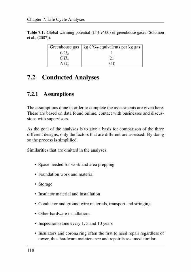
Chapter 7. Life Cycle Analyses
Table 7.1: Global warming potential (GWP100) of greenhouse gases (Solomonet al., (2007)).
Greenhouse gas kg CO2-equivalents per kg gasCO2 1CH4 21NOx 310
7.2 Conducted Analyses
7.2.1 Assumptions
The assumptions done in order to complete the assessments are given here.These are based on data found online, contact with businesses and discus-sions with supervisors.
As the goal of the analyses is to give a basis for comparison of the threedifferent designs, only the factors that are different are assessed. By doingso the process is simplified.
Similarities that are omitted in the analyses:
• Space needed for work and area prepping
• Foundation work and material
• Storage
• Insulator material and installation
• Conductor and ground wire materials, transport and stringing
• Other hardware installations
• Inspections done every 1, 5 and 10 years
• Insulators and corona ring often the first to need repair regardless oftower, thus hardware maintenance and repair is assumed similar.
118
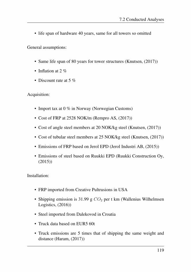
7.2 Conducted Analyses
• life span of hardware 40 years, same for all towers so omitted
General assumptions:
• Same life span of 80 years for tower structures (Knutsen, (2017))
• Inflation at 2 %
• Discount rate at 5 %
Acquisition:
• Import tax at 0 % in Norway (Norwegian Customs)
• Cost of FRP at 2528 NOK/m (Rempro AS, (2017))
• Cost of angle steel members at 20 NOK/kg steel (Knutsen, (2017))
• Cost of tubular steel members at 25 NOK/kg steel (Knutsen, (2017))
• Emissions of FRP based on Jerol EPD (Jerol Industri AB, (2015))
• Emissions of steel based on Ruukki EPD (Ruukki Construction Oy,(2015))
Installation:
• FRP imported from Creative Pultrusions in USA
• Shipping emission is 31.99 g CO2 per t km (Wallenius WilhelmsenLogistics, (2016))
• Steel imported from Dalekovod in Croatia
• Truck data based on EUR5 60t
• Truck emissions are 5 times that of shipping the same weight anddistance (Haram, (2017))
119

Chapter 7. Life Cycle Analyses
• Hourly rate of workers is 680 NOK/h
• Assembly time of guyed lattice steel tower (81298) 20 h/t (Knutsen,(2017))
• Assembly time of guyed tubular steel tower (76800) 10 h/t (Knutsen,(2017))
• Assembly time of guyed tubular FRP tower (48154) 9 h/t (Knutsen,(2017))
• Helicopter data based on Airbus H135 can lift 1000-1200 kg (AirbusHelicopters Inc, (2017))
• Hourly helicopter rate at 15000 NOK/h (Knutsen, (2017))
• Helicopter emissions are 3 kg CO2 per l fuel (Triple Pundit: Pablo,(2007))
• Helicopter use for lattice steel tower is 8 lifts of 10 min
• Helicopter use for tubular steel tower is 8 lifts of 10 min
• Helicopter use for tubular FRP tower is 5 lifts of 10 min
Use:
• Galvanized coating does not need refurbishment
• Repainting of steel every 20 years
• Cost of repainting is 3000 NOK/t (Knutsen, (2017))
• Transport is done by helicopter
• No refurbishment needed for FRP tower
Decommissioning:
• Deconstruction uses the same amount of time as assembly
120
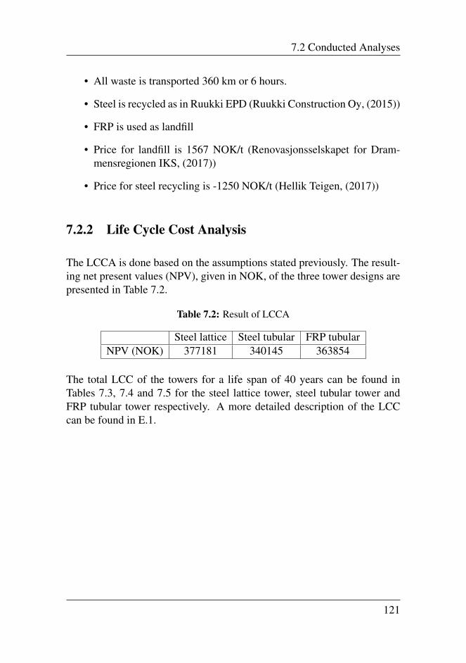
7.2 Conducted Analyses
• All waste is transported 360 km or 6 hours.
• Steel is recycled as in Ruukki EPD (Ruukki Construction Oy, (2015))
• FRP is used as landfill
• Price for landfill is 1567 NOK/t (Renovasjonsselskapet for Dram-mensregionen IKS, (2017))
• Price for steel recycling is -1250 NOK/t (Hellik Teigen, (2017))
7.2.2 Life Cycle Cost Analysis
The LCCA is done based on the assumptions stated previously. The result-ing net present values (NPV), given in NOK, of the three tower designs arepresented in Table 7.2.
Table 7.2: Result of LCCA
Steel lattice Steel tubular FRP tubularNPV (NOK) 377181 340145 363854
The total LCC of the towers for a life span of 40 years can be found inTables 7.3, 7.4 and 7.5 for the steel lattice tower, steel tubular tower andFRP tubular tower respectively. A more detailed description of the LCCcan be found in E.1.
121
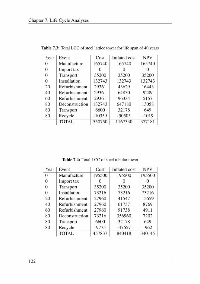
Chapter 7. Life Cycle Analyses
Table 7.3: Total LCC of steel lattice tower for life span of 40 years
Year Event Cost Inflated cost NPV0 Manufacture 165740 165740 1657400 Import tax 0 0 00 Transport 35200 35200 352000 Installation 132743 132743 13274320 Refurbishment 29361 43629 1644340 Refurbishment 29361 64830 920960 Refurbishment 29361 96334 515780 Deconstruction 132743 647180 1305880 Transport 6600 32178 64980 Recycle -10359 -50505 -1019
TOTAL 550750 1167330 377181
Table 7.4: Total LCC of steel tubular tower
Year Event Cost Inflated cost NPV0 Manufacture 195500 195500 1955000 Import tax 0 0 00 Transport 35200 35200 352000 Installation 73216 73216 7321620 Refurbishment 27960 41547 1565940 Refurbishment 27960 61737 876960 Refurbishment 27960 91738 491180 Deconstruction 73216 356960 720280 Transport 6600 32178 64980 Recycle -9775 -47657 -962
TOTAL 457837 840418 340145
122
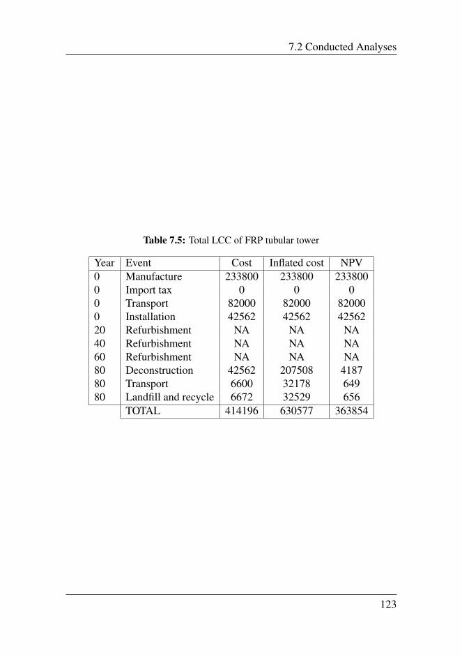
7.2 Conducted Analyses
Table 7.5: Total LCC of FRP tubular tower
Year Event Cost Inflated cost NPV0 Manufacture 233800 233800 2338000 Import tax 0 0 00 Transport 82000 82000 820000 Installation 42562 42562 4256220 Refurbishment NA NA NA40 Refurbishment NA NA NA60 Refurbishment NA NA NA80 Deconstruction 42562 207508 418780 Transport 6600 32178 64980 Landfill and recycle 6672 32529 656
TOTAL 414196 630577 363854
123
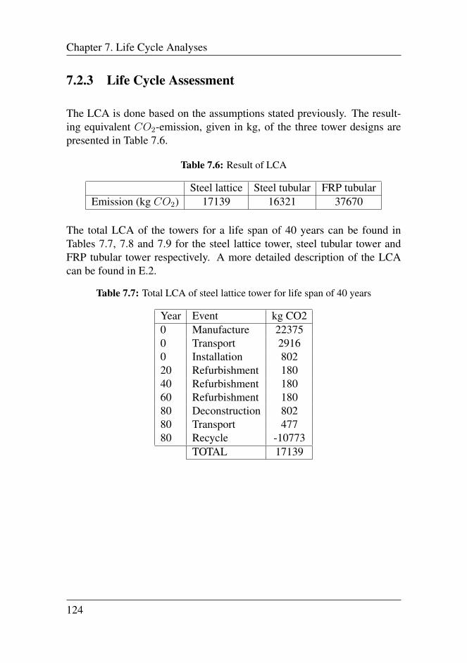
Chapter 7. Life Cycle Analyses
7.2.3 Life Cycle Assessment
The LCA is done based on the assumptions stated previously. The result-ing equivalent CO2-emission, given in kg, of the three tower designs arepresented in Table 7.6.
Table 7.6: Result of LCA
Steel lattice Steel tubular FRP tubularEmission (kg CO2) 17139 16321 37670
The total LCA of the towers for a life span of 40 years can be found inTables 7.7, 7.8 and 7.9 for the steel lattice tower, steel tubular tower andFRP tubular tower respectively. A more detailed description of the LCAcan be found in E.2.
Table 7.7: Total LCA of steel lattice tower for life span of 40 years
Year Event kg CO20 Manufacture 223750 Transport 29160 Installation 80220 Refurbishment 18040 Refurbishment 18060 Refurbishment 18080 Deconstruction 80280 Transport 47780 Recycle -10773
TOTAL 17139
124
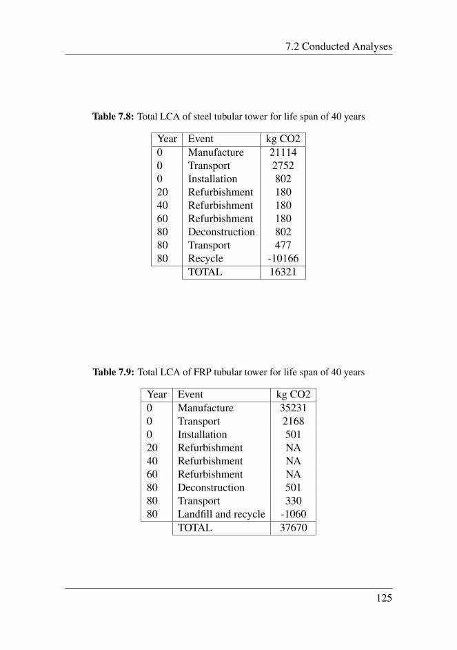
7.2 Conducted Analyses
Table 7.8: Total LCA of steel tubular tower for life span of 40 years
Year Event kg CO20 Manufacture 211140 Transport 27520 Installation 80220 Refurbishment 18040 Refurbishment 18060 Refurbishment 18080 Deconstruction 80280 Transport 47780 Recycle -10166
TOTAL 16321
Table 7.9: Total LCA of FRP tubular tower for life span of 40 years
Year Event kg CO20 Manufacture 352310 Transport 21680 Installation 50120 Refurbishment NA40 Refurbishment NA60 Refurbishment NA80 Deconstruction 50180 Transport 33080 Landfill and recycle -1060
TOTAL 37670
125


Chapter 8Discussion
8.1 Material Properties
The material properties for glass fibre reinforced polymers as given bySinha and Vinay ((2010)) are presented in Table 8.1, where they are alsocompared to concrete, steel and wood.
Table 8.1: Material properties of FRP, concrete, steel and wood.
Material FRP Steel Concrete TimberGlass fibre % 40-80 - - -Specific gravity 1.66-2.05 7.85 2.4 0.42-0.52Tensile strength (MPa) 200-1200 470-630 - -Tensile modulus (GPa) 19-32 210 - -Flexural strength (MPa) 200-1240 415-550 - 80Flexural modulus (GPa) 12-20 210 - 11-12Compressive strength (MPa) 200-480 220-250 20-60 17-50Thermal conductivity (W/mK) 0.27-4 45-55 0.4-1.8 0.8-0.19Coefficient of thermal expansion 7-10 6-12 10-15 1.7-2.5
Source: IPI (Indian Plastics Institute) Journal. 1998. p.21.
127
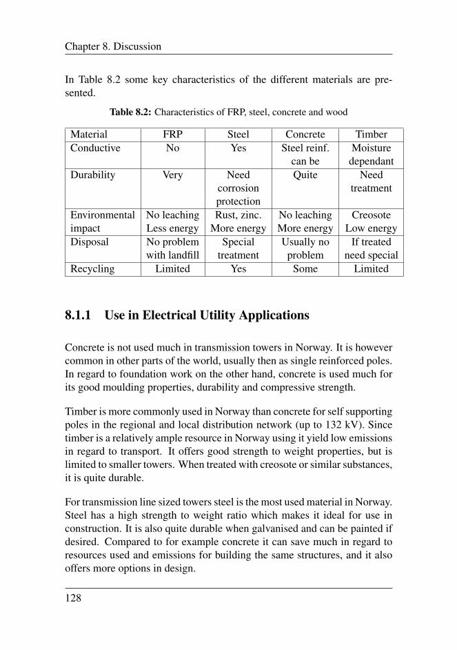
Chapter 8. Discussion
In Table 8.2 some key characteristics of the different materials are pre-sented.
Table 8.2: Characteristics of FRP, steel, concrete and wood
Material FRP Steel Concrete TimberConductive No Yes Steel reinf. Moisture
can be dependantDurability Very Need Quite Need
corrosion treatmentprotection
Environmental No leaching Rust, zinc. No leaching Creosoteimpact Less energy More energy More energy Low energyDisposal No problem Special Usually no If treated
with landfill treatment problem need specialRecycling Limited Yes Some Limited
8.1.1 Use in Electrical Utility Applications
Concrete is not used much in transmission towers in Norway. It is howevercommon in other parts of the world, usually then as single reinforced poles.In regard to foundation work on the other hand, concrete is used much forits good moulding properties, durability and compressive strength.
Timber is more commonly used in Norway than concrete for self supportingpoles in the regional and local distribution network (up to 132 kV). Sincetimber is a relatively ample resource in Norway using it yield low emissionsin regard to transport. It offers good strength to weight properties, but islimited to smaller towers. When treated with creosote or similar substances,it is quite durable.
For transmission line sized towers steel is the most used material in Norway.Steel has a high strength to weight ratio which makes it ideal for use inconstruction. It is also quite durable when galvanised and can be painted ifdesired. Compared to for example concrete it can save much in regard toresources used and emissions for building the same structures, and it alsooffers more options in design.
128
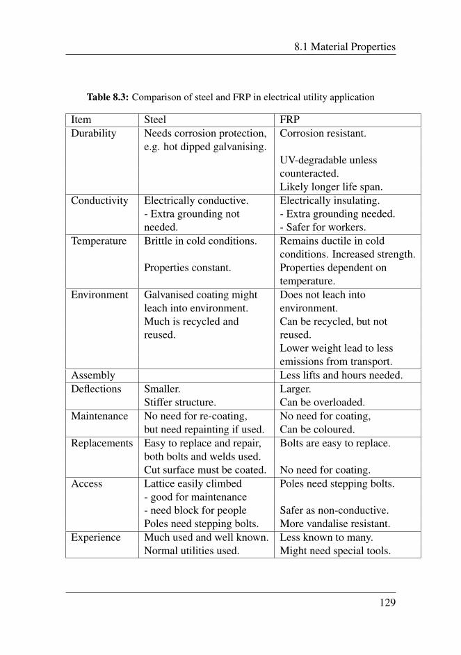
8.1 Material Properties
Table 8.3: Comparison of steel and FRP in electrical utility application
Item Steel FRPDurability Needs corrosion protection, Corrosion resistant.
e.g. hot dipped galvanising.UV-degradable unlesscounteracted.Likely longer life span.
Conductivity Electrically conductive. Electrically insulating.- Extra grounding not - Extra grounding needed.needed. - Safer for workers.
Temperature Brittle in cold conditions. Remains ductile in coldconditions. Increased strength.
Properties constant. Properties dependent ontemperature.
Environment Galvanised coating might Does not leach intoleach into environment. environment.Much is recycled and Can be recycled, but notreused. reused.
Lower weight lead to lessemissions from transport.
Assembly Less lifts and hours needed.Deflections Smaller. Larger.
Stiffer structure. Can be overloaded.Maintenance No need for re-coating, No need for coating,
but need repainting if used. Can be coloured.Replacements Easy to replace and repair, Bolts are easy to replace.
both bolts and welds used.Cut surface must be coated. No need for coating.
Access Lattice easily climbed Poles need stepping bolts.- good for maintenance- need block for people Safer as non-conductive.Poles need stepping bolts. More vandalise resistant.
Experience Much used and well known. Less known to many.Normal utilities used. Might need special tools.
129
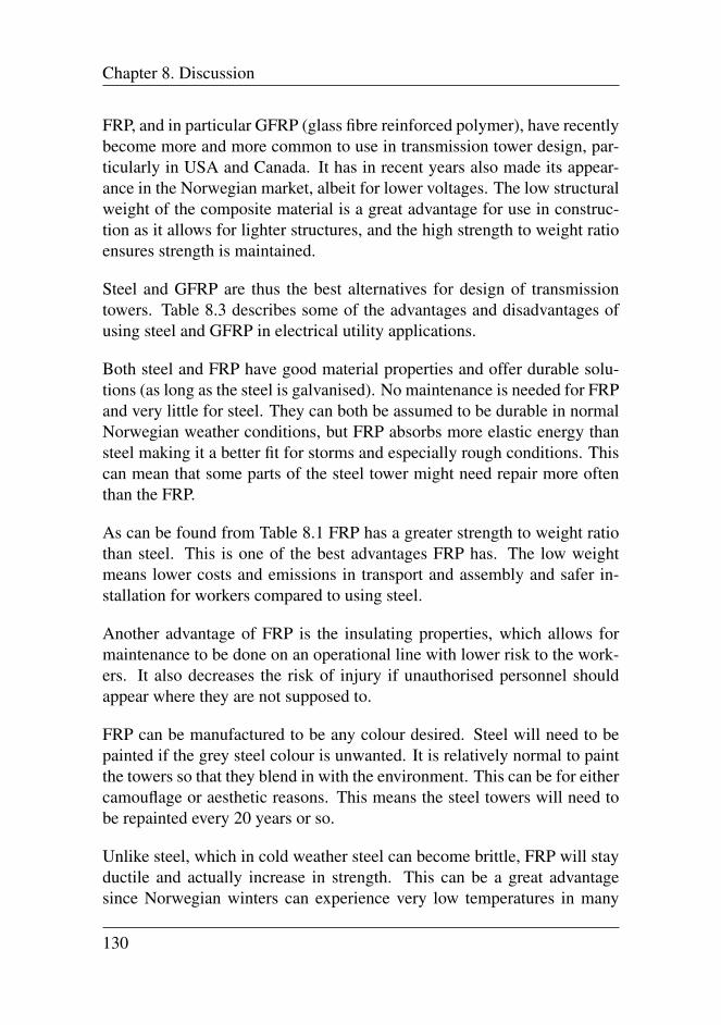
Chapter 8. Discussion
FRP, and in particular GFRP (glass fibre reinforced polymer), have recentlybecome more and more common to use in transmission tower design, par-ticularly in USA and Canada. It has in recent years also made its appear-ance in the Norwegian market, albeit for lower voltages. The low structuralweight of the composite material is a great advantage for use in construc-tion as it allows for lighter structures, and the high strength to weight ratioensures strength is maintained.
Steel and GFRP are thus the best alternatives for design of transmissiontowers. Table 8.3 describes some of the advantages and disadvantages ofusing steel and GFRP in electrical utility applications.
Both steel and FRP have good material properties and offer durable solu-tions (as long as the steel is galvanised). No maintenance is needed for FRPand very little for steel. They can both be assumed to be durable in normalNorwegian weather conditions, but FRP absorbs more elastic energy thansteel making it a better fit for storms and especially rough conditions. Thiscan mean that some parts of the steel tower might need repair more oftenthan the FRP.
As can be found from Table 8.1 FRP has a greater strength to weight ratiothan steel. This is one of the best advantages FRP has. The low weightmeans lower costs and emissions in transport and assembly and safer in-stallation for workers compared to using steel.
Another advantage of FRP is the insulating properties, which allows formaintenance to be done on an operational line with lower risk to the work-ers. It also decreases the risk of injury if unauthorised personnel shouldappear where they are not supposed to.
FRP can be manufactured to be any colour desired. Steel will need to bepainted if the grey steel colour is unwanted. It is relatively normal to paintthe towers so that they blend in with the environment. This can be for eithercamouflage or aesthetic reasons. This means the steel towers will need tobe repainted every 20 years or so.
Unlike steel, which in cold weather steel can become brittle, FRP will stayductile and actually increase in strength. This can be a great advantagesince Norwegian winters can experience very low temperatures in many
130
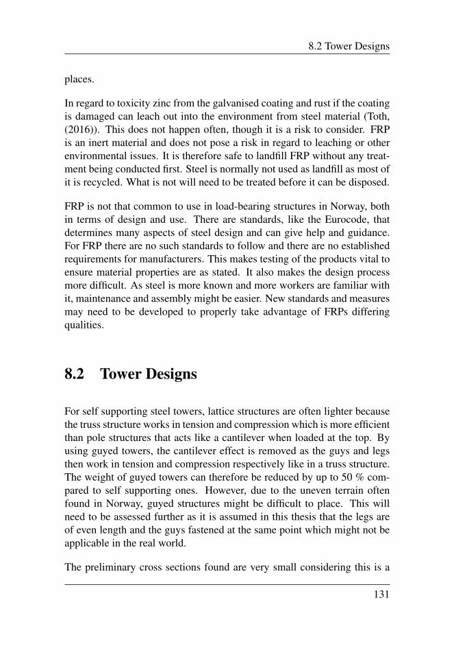
8.2 Tower Designs
places.
In regard to toxicity zinc from the galvanised coating and rust if the coatingis damaged can leach out into the environment from steel material (Toth,(2016)). This does not happen often, though it is a risk to consider. FRPis an inert material and does not pose a risk in regard to leaching or otherenvironmental issues. It is therefore safe to landfill FRP without any treat-ment being conducted first. Steel is normally not used as landfill as most ofit is recycled. What is not will need to be treated before it can be disposed.
FRP is not that common to use in load-bearing structures in Norway, bothin terms of design and use. There are standards, like the Eurocode, thatdetermines many aspects of steel design and can give help and guidance.For FRP there are no such standards to follow and there are no establishedrequirements for manufacturers. This makes testing of the products vital toensure material properties are as stated. It also makes the design processmore difficult. As steel is more known and more workers are familiar withit, maintenance and assembly might be easier. New standards and measuresmay need to be developed to properly take advantage of FRPs differingqualities.
8.2 Tower Designs
For self supporting steel towers, lattice structures are often lighter becausethe truss structure works in tension and compression which is more efficientthan pole structures that acts like a cantilever when loaded at the top. Byusing guyed towers, the cantilever effect is removed as the guys and legsthen work in tension and compression respectively like in a truss structure.The weight of guyed towers can therefore be reduced by up to 50 % com-pared to self supporting ones. However, due to the uneven terrain oftenfound in Norway, guyed structures might be difficult to place. This willneed to be assessed further as it is assumed in this thesis that the legs areof even length and the guys fastened at the same point which might not beapplicable in the real world.
The preliminary cross sections found are very small considering this is a
131
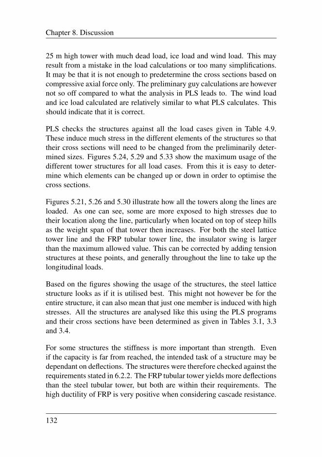
Chapter 8. Discussion
25 m high tower with much dead load, ice load and wind load. This mayresult from a mistake in the load calculations or too many simplifications.It may be that it is not enough to predetermine the cross sections based oncompressive axial force only. The preliminary guy calculations are howevernot so off compared to what the analysis in PLS leads to. The wind loadand ice load calculated are relatively similar to what PLS calculates. Thisshould indicate that it is correct.
PLS checks the structures against all the load cases given in Table 4.9.These induce much stress in the different elements of the structures so thattheir cross sections will need to be changed from the preliminarily deter-mined sizes. Figures 5.24, 5.29 and 5.33 show the maximum usage of thedifferent tower structures for all load cases. From this it is easy to deter-mine which elements can be changed up or down in order to optimise thecross sections.
Figures 5.21, 5.26 and 5.30 illustrate how all the towers along the lines areloaded. As one can see, some are more exposed to high stresses due totheir location along the line, particularly when located on top of steep hillsas the weight span of that tower then increases. For both the steel latticetower line and the FRP tubular tower line, the insulator swing is largerthan the maximum allowed value. This can be corrected by adding tensionstructures at these points, and generally throughout the line to take up thelongitudinal loads.
Based on the figures showing the usage of the structures, the steel latticestructure looks as if it is utilised best. This might not however be for theentire structure, it can also mean that just one member is induced with highstresses. All the structures are analysed like this using the PLS programsand their cross sections have been determined as given in Tables 3.1, 3.3and 3.4.
For some structures the stiffness is more important than strength. Evenif the capacity is far from reached, the intended task of a structure may bedependant on deflections. The structures were therefore checked against therequirements stated in 6.2.2. The FRP tubular tower yields more deflectionsthan the steel tubular tower, but both are within their requirements. Thehigh ductility of FRP is very positive when considering cascade resistance.
132
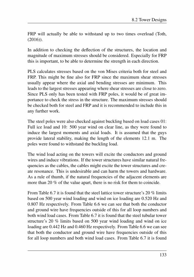
8.2 Tower Designs
FRP will actually be able to withstand up to two times overload (Toth,(2016)).
In addition to checking the deflection of the structures, the location andmagnitude of maximum stresses should be considered. Especially for FRPthis is important, to be able to determine the strength in each direction.
PLS calculates stresses based on the von Mises criteria both for steel andFRP. This might be fine also for FRP since the maximum shear stressesusually appear where the axial and bending stresses are minimum. Thisleads to the largest stresses appearing where shear stresses are close to zero.Since PLS only has been tested with FRP poles, it would be of great im-portance to check the stress in the structure. The maximum stresses shouldbe checked both for steel and FRP and it is recommended to include this inany further work.
The steel poles were also checked against buckling based on load cases 01:Full ice load and 10: 500 year wind on clear line, as they were found toinduce the largest moments and axial loads. It is assumed that the guysprovide lateral stability, making the length of the elements 12.1 m. Thepoles were found to withstand the buckling load.
The wind load acting on the towers will excite the conductors and groundwires and induce vibrations. If the tower structures have similar natural fre-quencies as the cables, the cables might excite the tower structures and cre-ate resonance. This is undesirable and can harm the towers and hardware.As a rule of thumb, if the natural frequencies of the adjacent elements aremore than 20 % of the value apart, there is no risk for them to coincide.
From Table 6.7 it is found that the steel lattice tower structure’s 20 % limitsbased on 500 year wind loading and wind on ice loading are 0.520 Hz and0.807 Hz respectively. From Table 6.6 we can see that both the conductorand ground wire have frequencies outside of this for all loop numbers andboth wind load cases. From Table 6.7 it is found that the steel tubular towerstructure’s 20 % limits based on 500 year wind loading and wind on iceloading are 0.442 Hz and 0.460 Hz respectively. From Table 6.6 we can seethat both the conductor and ground wire have frequencies outside of thisfor all loop numbers and both wind load cases. From Table 6.7 it is found
133
Chapter 8. Discussion
that the FRP tubular tower structure’s 20 % limits based on 500 year windloading and wind on ice loading are 0.378 Hz and 0.420 Hz respectively.From Table 6.6 we can see that both the conductor and ground wire havefrequencies outside of this for all loop numbers and both wind load cases.
All towers are thus adequate when checked for these wind loads. It mightbe relevant to check vibrations other set up by other wind velocities to seeif they induce resonance. For example for lower wind velocities to checkagainst aeolian vibrations.
8.3 LCCA and LCA
LCAs and LCCAs are done based on many assumptions and uncertain fac-tors. It can be a hard task to correctly judge the different aspects of theanalyses and experience is therefore key.
Since not all tower elements and life phases are included in the analyses, theresults are only applicable under the stated conditions and to the materialschosen. When assessing the results it is important to keep this in mind asthe differences found will make a lower impact when looking at the systemas a whole, both for the LCCA and the LCA.
The steel elements used in the analysis are assumed produced by Dalekovod,which is one of the manufacturers used by Statnett today. Another one isMitas, located in Turkey. Choosing a different manufacturer will changesome of the costs and emissions in regard to transport, unless the deliverycost to Norway is included in the material cost. There are other manufac-turers in Norway or closer such as Skanska, Contiga and Ruukki, but theseare normally not used for the transmission network. They may howeverbe relevant for the regional or distribution network. Ruukki’s EPD for hotrolled steel elements is used as a basis for the LCA calculations, as well asthe ones from Skanska and Contiga.
The FRP elements also have some uncertainty in regard to the transportpart. When assuming they are produced in the US, extra costs and emis-sions are added by requiring longer transport stretches. However, as tech-
134
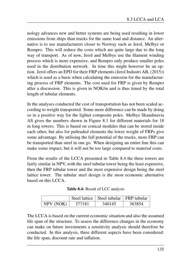
8.3 LCCA and LCA
nology advances new and better systems are being used resulting in loweremissions from ships than trucks for the same load and distance. An alter-native is to use manufacturers closer to Norway such as Jerol, Melbye orRempro. This will reduce the costs which are quite large due to the longway of transport. As of now, Jerol and Melbye use the filament windingprocess which is more expensive, and Rempro only produce smaller polesused in the distribution network. In time this might however be an op-tion. Jerol offers an EPD for their FRP elements (Jerol Industri AB, (2015))which is used as a basis when calculating the emission for the manufactur-ing process of FRP elements. The cost used for FRP is given by Remproafter a discussion. This is given in NOK/m and is thus timed by the totallength of tubular elements.
In the analyses conducted the cost of transportation has not been scaled ac-cording to weight transported. Some more difference can be made by doingso in a positive way for the lighter composite poles. Melbye SkandinaviaAS gives the numbers shown in Figure 8.1 for different materials for 18m long towers. This is based on conical modules that can be stored insideeach other, but also for pultruded elements the lower weight of FRPs givesome advantage. By utilising the full potential of the trucks, more FRP canbe transported than steel in one go. When designing an entire line this canmake some impact, but it will not be too large compared to material costs.
From the results of the LCCA presented in Table 8.4 the three towers arefairly similar in NPV, with the steel tubular tower being the least expensive,then the FRP tubular tower and the most expensive design being the steellattice tower. The tubular steel design is the most economic alternativebased on this LCCA.
Table 8.4: Result of LCC analysis
Steel lattice Steel tubular FRP tubularNPV (NOK) 377181 340145 363854
The LCCA is based on the current economic situation and also the assumedlife span of the structure. To assess the difference changes in the economycan make on future investments a sensitivity analysis should therefore beconducted. In this analysis, three different aspects have been considered:the life span, discount rate and inflation.
135
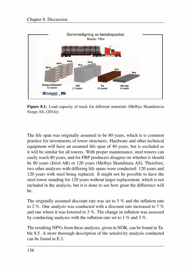
Chapter 8. Discussion
Figure 8.1: Load capacity of truck for different materials (Melbye SkandinaviaNorge AS, (2014))
The life span was originally assumed to be 80 years, which is is commonpractice for investments of tower structures. Hardware and other technicalequipment will have an assumed life span of 40 years, but is excluded asit will be similar for all towers. With proper maintenance, steel towers caneasily reach 80 years, and for FRP producers disagree on whether it shouldbe 80 years (Jerol AB) or 120 years (Melbye Skandinaia AS). Therefore,two other analyses with differing life spans were conducted: 120 years and120 years with steel being replaced. It might not be possible to have thesteel tower standing for 120 years without larger replacement, which is notincluded in the analysis, but it is done to see how great the difference willbe.
The originally assumed discount rate was set to 5 % and the inflation rateto 2 %. One analysis was conducted with a discount rate increased to 7 %and one where it was lowered to 3 %. The change in inflation was assessedby conducting analyses with the inflation rate set to 1 % and 3 %.
The resulting NPVs from these analyses, given in NOK, can be found in Ta-ble 8.5. A more thorough description of the sensitivity analysis conductedcan be found in E.3.
136
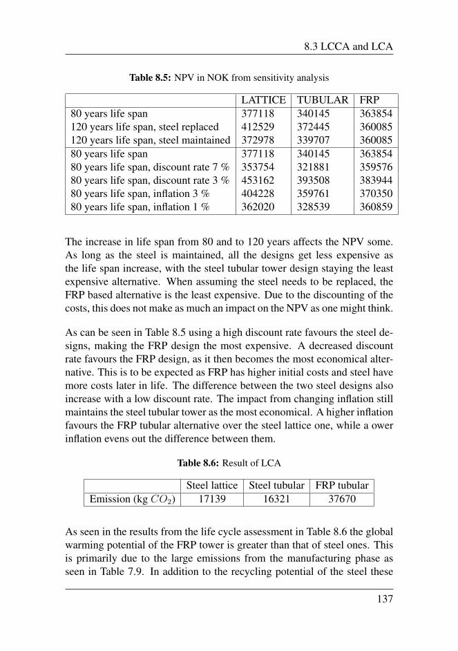
8.3 LCCA and LCA
Table 8.5: NPV in NOK from sensitivity analysis
LATTICE TUBULAR FRP80 years life span 377118 340145 363854120 years life span, steel replaced 412529 372445 360085120 years life span, steel maintained 372978 339707 36008580 years life span 377118 340145 36385480 years life span, discount rate 7 % 353754 321881 35957680 years life span, discount rate 3 % 453162 393508 38394480 years life span, inflation 3 % 404228 359761 37035080 years life span, inflation 1 % 362020 328539 360859
The increase in life span from 80 and to 120 years affects the NPV some.As long as the steel is maintained, all the designs get less expensive asthe life span increase, with the steel tubular tower design staying the leastexpensive alternative. When assuming the steel needs to be replaced, theFRP based alternative is the least expensive. Due to the discounting of thecosts, this does not make as much an impact on the NPV as one might think.
As can be seen in Table 8.5 using a high discount rate favours the steel de-signs, making the FRP design the most expensive. A decreased discountrate favours the FRP design, as it then becomes the most economical alter-native. This is to be expected as FRP has higher initial costs and steel havemore costs later in life. The difference between the two steel designs alsoincrease with a low discount rate. The impact from changing inflation stillmaintains the steel tubular tower as the most economical. A higher inflationfavours the FRP tubular alternative over the steel lattice one, while a owerinflation evens out the difference between them.
Table 8.6: Result of LCA
Steel lattice Steel tubular FRP tubularEmission (kg CO2) 17139 16321 37670
As seen in the results from the life cycle assessment in Table 8.6 the globalwarming potential of the FRP tower is greater than that of steel ones. Thisis primarily due to the large emissions from the manufacturing phase asseen in Table 7.9. In addition to the recycling potential of the steel these
137
Chapter 8. Discussion
constitute a great difference. The advantages the low weight give in trans-portation and assembly are not enough to close the gap. In regard to wastemanagement of the decommissioned towers, it is assumed that most of thesteel is recycled. FRPs are assumed to be land filled, and as there are noemissions from FRP to air or water this is a good solution.
However, since the emissions in the production phase are so large, it wouldbe better to recycle the FRP. As discussed by Shuaib and Mativenga ((2016))recovering products from waste uses much less energy than producing vir-gin materials. Thus by recycling the FRPs as well the carbon footprint canbe reduced. This is based on a process where the materials are granulatedwhich means they cannot be used in the same way as before as the fibres nolonger are clean and long. Some research is being conducted on fungi andpolymers to assess the possibility of recycling the glass fibres while keep-ing them intact. In the future this might be a possibility, which can greatlyreduce the global warming potential as seen in Table 7.9. The expectation isthat by the time of the commissioning of these towers, complete recyclingof FRP will be possible (Toth, (2016)).
An assessment done by Erlandsson (2011)) also considers different mate-rials used for utility poles, including both concrete and wood in additionto steel and FRP. This assessment considers more types of environmentalimpact than just CO2-equivalents. It is found that FRP generally scoressimilarly or better than steel. Especially considering human toxicity it isbetter.
If the assumed life span was increased so that the steel would have to be re-placed and not the FRP, the environmental impact of the steel towers wouldalmost be similar to that of the FRP. This could likely happen if one isto trust manufacturers and if so these results should not make as great animpact on the decision.
138
Chapter 9Conclusion
Both steel and FRP offer good material properties for use in transmissiontowers. Their properties are in many cases similar, but the insulating abili-ties and low weight of FRP does give it an advantage relative to steel.
All the three different tower designs with the chosen dimensions are foundto be of sufficient strength.
Based on the life cycle cost analysis conducted the steel tubular tower offersthe most economic design, with the FRP tubular tower as the second mosteconomic. The most expensive tower design is the steel lattice tower.
From the environmental life cycle assessment conducted one can see thatthe designs using steel offers the most environmentally friendly alterna-tives, with the tubular design being the best one. The FRP tubular towerdesign scores lower when it comes to environmental impact as the emis-sions of CO2-equivalents is the highest of the three by about the double ofthe others.
The sensitivity of the analyses in regard to inflation and life span is deemedquite low as the results stay mostly the same when these parameters arechanged. Using a lower discount rate will however change the outcomeand must be considered.
139
Chapter 9. Conclusion
Based on this, the conclusion is that FRP can make a good alternative tothe traditional use of steel in transmission towers, particularly when con-sidering the life cycle costs. The initial cost however, is lower for the steeldesigns. Developing new and efficient recycling processes of FRP and rou-tines and standardisations for its use and design, can lead to FRP becominga better alternative in the future, particularly in regard to emissions.
For the time being, the steel tubular tower design is considered a betteralternative when both life cycle cost and environmental impact are consid-ered.
Some further work that can be assessed:- detailed connection design- optimising span length in regard to cost by comparing costs for differenttower heights- hand calculations of stresses in the tower members and buckling of FRP-poles
140
Bibliography
Airbus Helicopters Inc, (2017). H135 (formerly known as EC135) specifi-cations. (Used: 20. December 2016).URL http://airbushelicoptersinc.com/products/H135-specifications.asp
Akovali, G., Uyanik, N., Kaynak, C., Akgul, T., Kenig, S., Parnas, L.,Ardic, S., Giordano, M., Borzacchiello, A., Nicolais, L., Elaldi, F.,(2001). Handbook of Composite Fabrication. Rapra Technology Lim-ited, UK.
Alfredsen, K., Brattebø, H., Heie, A., Killingtveit, A., Lia, L., Renaas, M.,Sægrov, S., Thorolfsson, S. T., Østerhus, S. W., (2012). KompendiumTVM4101 BM2 Vann- og miljøteknikk. NTNU - IVT - IVM.
Blevins, R. D., (2016). Formulas for Dynamics, Acoustics and Vibration,1st Edition. John Wiley & Sons, Ltd.
Brown, R., (2002). Handbook of Polymer Testing. Rapra Technology Ltd.
Catchpole, P., Fife, B., (2014). Structural Engineering of TransmissionLines. ICE Publishing.
CEN, (2005). NS-EN 1993-1-1:2005+NA:2008: Prosjektering avstalkonstruksjoner - Del 1-1: Allmenne regler og regler for bygninger.Standard Norge.
CENELEC, (2012). FprEN 50341-1:2012 Overhead electrical lines ex-ceeding AC 1 kV - Part 1: General requirements - Common specifica-tions. CENELEC - European Committee for Electrotechnical Standard-ization.
141

Dudok van Heel, D., Maas, T., De Gijt, J., Said, M., (2011). Comparisonof Infrastructure Designs for Quay Wall and Small Bridges in Concrete,Steel, Wood and Composites with Regard to the CO2-Emission and theLife Cycle Analysis, the 3rd International Conference of EACEF.
Duflou, J. R., Deng, Y., Van Acker, K., Dewulf, W., (2012). Do fiber-reinforced polymer composites provide environmentally benign alterna-tives? A life-cycle-assessment-based study. MRS Bulletin 37 (4), 374–382.
Erlandsson, M., 2011. Comparison of the environmental impacts from util-ity poles in different materials - a life cycle assessment. Tech. rep., IVLSwedish Environmental Research Institute AB.
Gani, F., Legeron, F., (2010). Dynamic response of transmission lines guyedtowers under wind loading. Canadian Journal of Civil Engineering 37,450–464.
Halliwell, S., (2002). Polymers in Buildings and Structures. Rapra Tech-nology Ltd.
Haram, H. K., (2017). Mye mindre CO2 via sjø. (Used: 20. December2016).URL http://old.shortseashipping.no/sitepages/News.aspx?t=Mye+mindre+CO2+via+sj%C3%B8
Hellik Teigen, January (2017). Private communication.
Huntsman International LLC1, (2013). Video - How it works: FilamentWinding. (Used: 10. October 2016).URL https://www.youtube.com/watch?v=ign6W5ENJAA
Huntsman International LLC2, (2016). Video - Pultrusion. (Used: 10. Oc-tober 2016).URL https://www.youtube.com/watch?v=YFyvCf322_g
Jerol Industri AB, (2015). Kap. 11. Miljoaspekter – arbetsmiljo ochmarkmiljo. (Used: 23. November 2016).URL http://jerol.se/wp-content/uploads/2014/11/Kap11_Miljoaspekter_2015-11-05.pdf
142
Kendall, D., unknown. Fibre Reinforced Polymer (FRP) Composite Build-ings - Future Opportunities. National Composites Network.
Kiessling, F., Nefzger, P., Nolasco, J. F., Kaintzyk, U., (2003). OverheadPower Lines. Springer.
Knutsen, R. G., January (2017). Private communication.
Larsen, P. K., (2015). Dimensjonering av stalkonstruksjoner. Fagbokfor-laget Vigmostad og Bjørke AS, Norway.
Lilien, J.-L., (2013). Power Line Aeolian Vibrations. Tech. rep., Departmentof Electronics, Electricity and Computer Sciences, University of Liege.
Melbye Skandinavia Norge AS, (2014). Komposittmaster - Fremtidensløsning i dag. (Used: 10. September 2016).URL http://www.melbye.com/melbye/frontend/mediabank/2294/Komposittmaster-web.pdf
Peters, S. T., (2011). Composite Filament Winding. ASM International.
Power Line Systems Inc1, (Updated 2016). PLS-CADD (Power LineSystems - Computer Aided Design and Drafting). (Used: 16. September2016).URL https://www.powline.com/products/pls_cadd.html
Power Line Systems Inc3, (Updated 2016). PLS-POLE (Power LineSystems - Computer Aided Design and Drafting). (Used: 16. September2016).URL https://www.powline.com/products/pls_pole.html
Power Line Systems Inc4, (2016). PLS-CADD User’s Manual, version14.2.
Power Line Systems Inc5, (2016). PLS-POLE User’s Manual, version 14.2.
Power Line Systems Inc6, (2016). PLS-TOWER User’s Manual, version14.2.
143
Power Line SystemsI nc2, (Updated 2016). PLS-TOWER (Power Line Sys-tems - Computer Aided Design and Drafting). (Used: 16. September2016).URL https://www.powline.com/products/tower.html
Preformed Line Products, (2016). Conductor Galloping Basics. (Used: 19.December 2016).URL http://www.preformed.com/images/pdfs/Energy/Transmission/Motion_Control/Detuning_Pendulum/Conductor_Galloping_Basics-EN-ML-1166.pdf
Remer, D. S., Nieto, A. P., (1995). A compendium and comparison of 25project evaluation techniques. Part 1: Net present value and rate of re-turn methods. International Journal of Production Economics 42, 79–96.
Rempro AS, January (2017). Private communication.
Renovasjonsselskapet for Drammensregionen IKS, (2017). Prisliste for lev-ering av næringsavfall. (Used: 20. December 2016).URL http://www.rfd.no/bedrift/bli-bedriftskunde/priser/prisliste
Ruukki Construction Oy, (2015). NEPD-324-204-EN Welded and coatedsections, trusses and beams made of hot-rolled plate, sheet and coil.
Shuaib, N. A., Mativenga, P. T., (2016). Energy demand in mechanicalrecycling of glass fibre reinforced thermoset plastic composites. Journalof Cleaner Production 120, 198–206.
Sinha, S., Vinay, K., (2010). Polymeric Systems and Applications. StudiumPress (India) Pvt. Ltd.
Solomon, S., Qin, D., Manning, M., Alley, R. B., Berntsen, T., Bind-off, N. L., Chen, Z., Chidthaisong, A., Gregory, J. M., Hegerl, G. C.,Heimann, M., Hewitson, B., Hoskins, B. J., Joos, F., Jouzel, J., Kattsov,V., Lohmann, U., Matsuno, T., Molina, M., Nicholls, N., Overpeck,J., Raga, G., Ramaswamy, V., Ren, J., Rusticucci, M., Somerville, R.,Stocker, T. F., Whetton, P., Wood, R. A., Wratt, D., (2007). TechnicalSummary. Climate Change 2007: The Physical Science Basis. Contribu-tion of Working Group I to the Fourth Assessment Report of the Inter-governmental Panel on Climate Change.
144
Statnett SF, (2016). About us - Statnett. (Used: 22. November 2016).URL http://www.statnett.no/en/About-Statnett/
The Environmental Literacy Council, (2015). Life Cycle Analysis. (Used:23. November 2016).URL https://enviroliteracy.org/environment-society/life-cycle-analysis/
The Norwegian EPD Foundation, (2016). Hva er en EPD? (Used: 25.November 2016).URL http://epd-norge.no/hva-er-en-epd/
The Norwegian National Committee, (2008). NO NNA-EN 50341-3-16:2008: National Normative Aspects for Norway. CENELEC - Euro-pean Committee for Electrotechnical Standardization.
The Physics Classroom, (1996-2016). Natural Frequency. (Used: 19. De-cember 2016).URL http://www.physicsclassroom.com/class/sound/Lesson-4/Natural-Frequency
Toth, J., September (2016). Private communication.
Triple Pundit: Pablo, (2007). AskPablo: Helicopter Emissions. (Used: 20.December 2016).URL http://www.triplepundit.com/2007/10/askpablo-helicopter-emissions/
Vinson, J. R., Sierakowski, R. L., (1993). The behaviour of structures com-posed of composite materials. Kluwer Academic Publishers.
Vinson, J. R., Sierakowski, R. L., (2012). The Behaviour of Structures Com-posed of Composite Materials, 2nd Edition. Kluwer Academic Publish-ers.
Wallenius Wilhelmsen Logistics, (2016). Sustainability report 2015.(Used: 20. December 2016).URL http://www.2wglobal.com/news-and-insights/infographics/sustainability-report-2015/#.WH9juIWcHIU
145
White, H. B., (1993). Guyed structures for transmission lines. EngineeringStructures 15 (4), 289–302.
Woodward, D. G., (1997). Life cycle costing - theory, information ac-quisition and application. International Journal of Project Management15 (6), 335–344.
Wubbenhorst, K. L., (1986). Life Cycle Costing for Construction Projects.Long Range Planning 19 (4), 87–97.
146
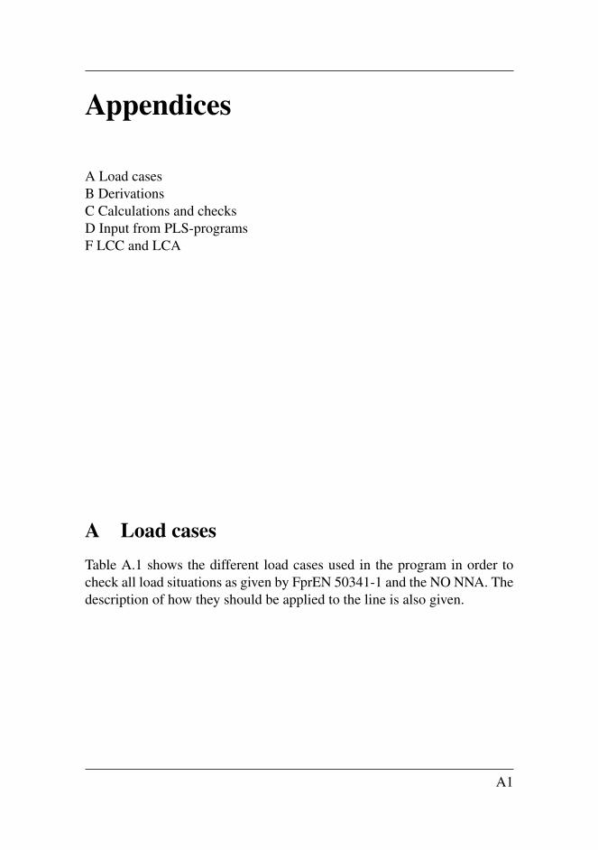
Appendices
A Load casesB DerivationsC Calculations and checksD Input from PLS-programsF LCC and LCA
A Load casesTable A.1 shows the different load cases used in the program in order tocheck all load situations as given by FprEN 50341-1 and the NO NNA. Thedescription of how they should be applied to the line is also given.
A1
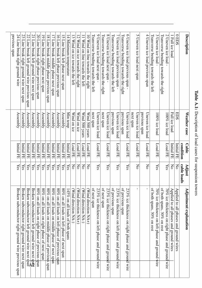
TableA
.1:D
escriptionofload
casesforsuspension
towers
Description
Weather
caseC
ableA
djustA
djustmentexplanation
conditioncable
loads0
ED
SE
DS
InitialFEN
oA
ppliedto
allphasesand
groundw
ires1
Fulliceload
Fulliceload
InitialFEN
oA
ppliedto
allphasesand
groundw
ires2
Uneven
iceload
-100%
iceload
Load
FEY
es70%
icethickness
onrightphase
andground
wire
Transversebending
towards
theright
ofbothspans,30%
onrest
3U
nevenice
load-
100%ice
loadL
oadFE
Yes
70%ice
thicknesson
leftphaseand
groundw
ireTransverse
bendingtow
ardsthe
leftofboth
spans,30%on
rest4
Uneven
iceload
previousspan
Uneven
iceload
Load
FEN
o-
previousspan
5U
nevenice
loadnextspan
Uneven
iceload
Load
FEN
o-
nextspan6
Uneven
iceload
previousspan
-U
nevenice
loadL
oadFE
Yes
233%ice
thicknesson
rightphaseand
groundw
ireTransverse
bendingtow
ardsthe
rightprevious
spanofprevious
span7
Uneven
iceload
previousspan
-U
nevenice
loadL
oadFE
Yes
233%ice
thicknesson
leftphaseand
groundw
ireTransverse
bendingtow
ardsthe
leftprevious
spanofprevious
span8
Uneven
iceload
nextspan-
Uneven
iceload
Load
FEY
es233%
icethickness
onrightphase
andground
wire
Transversebending
towards
theright
nextspanofnextspan
9U
nevenice
loadnextspan
-U
nevenice
loadL
oadFE
Yes
233%ice
thicknesson
leftphaseand
groundw
ireTransverse
bendingtow
ardsthe
leftnextspan
ofnextspan10
Wind
online
towards
theright
Wind
500years
Load
FEN
o(W
inddirection
NA
+)11
Wind
online
towards
theleft
Wind
500years
Load
FEN
o(W
inddirection
NA
-)12
Wind
onice
towards
theright
Wind
onice
Load
FEN
o(W
inddirection
NA
+)13
Wind
onice
towards
theleft
Wind
onice
Load
FEN
o(W
inddirection
NA
-)14
Minim
umtem
peratureM
intem
pInitialFE
Yes
145%on
allloadsofboth
spans15
Line
breakleftphase
nextspanA
ssembly
InitialFEY
es80%
onallloads
onleftphase
ofnextspan16
Line
breakleftphase
previousspan
Assem
blyInitialFE
Yes
80%on
allloadson
leftphaseofprevious
span17
Line
breakm
iddlephase
nextspanA
ssembly
InitialFEY
es80%
onallloads
onm
iddlephase
ofnextspan18
Line
breakm
iddlephase
previousspan
Assem
blyInitialFE
Yes
80%on
allloadson
middle
phaseofprevious
span19
Line
breakrightphase
nextspanA
ssembly
InitialFEY
es80%
onallloads
onrightphase
ofnextspan20
Line
breakrightphase
previousspan
Assem
blyInitialFE
Yes
80%on
allloadson
rightphaseofprevious
span21
Line
breakleftground
wire
nextspanA
ssembly
InitialFEY
esB
rokensubconductorleftground
wire
nextspan22
Line
breakleftground
wire
previousspan
Assem
blyInitialFE
Yes
Broken
subconductorleftgroundw
irenextspan
23L
inebreak
rightgroundw
irenextspan
Assem
blyInitialFE
Yes
Broken
subconductorrightgroundw
irenextspan
24L
inebreak
rightgroundw
ireA
ssembly
InitialFEY
esB
rokensubconductorrightground
wire
previousspan
previousspan
A2
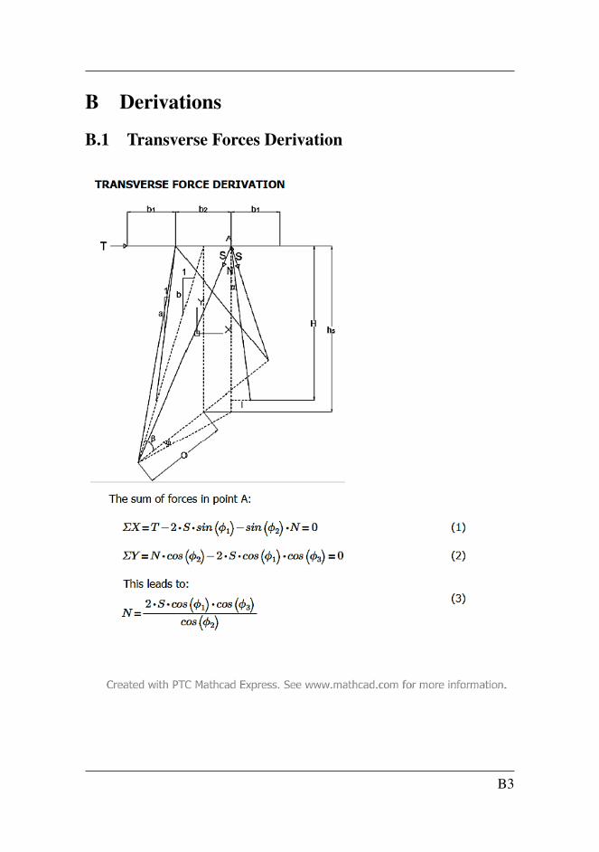
B Derivations
B.1 Transverse Forces Derivation
B3
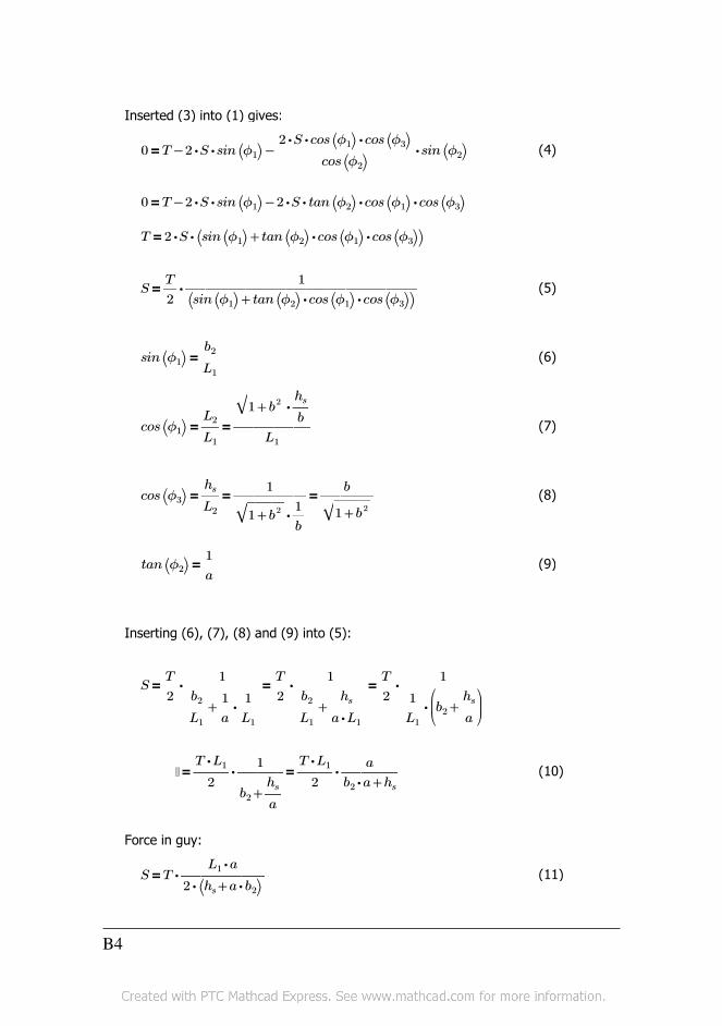
Inserted (3) into (1) gives:
=0 −−T ⋅⋅2 S sin ⎛⎝ϕ1⎞⎠ ⋅―――――――⋅⋅⋅2 S cos ⎛⎝ϕ1⎞⎠ cos ⎛⎝ϕ3⎞⎠
cos ⎛⎝ϕ2⎞⎠sin ⎛⎝ϕ2⎞⎠ (4)
=0 −−T ⋅⋅2 S sin ⎛⎝ϕ1⎞⎠ ⋅⋅⋅⋅2 S tan ⎛⎝ϕ2⎞⎠ cos ⎛⎝ϕ1⎞⎠ cos ⎛⎝ϕ3⎞⎠
=T ⋅⋅2 S ⎛⎝ +sin ⎛⎝ϕ1⎞⎠ ⋅⋅tan ⎛⎝ϕ2⎞⎠ cos ⎛⎝ϕ1⎞⎠ cos ⎛⎝ϕ3⎞⎠⎞⎠
=S ⋅―T
2――――――――――――
1⎛⎝ +sin ⎛⎝ϕ1⎞⎠ ⋅⋅tan ⎛⎝ϕ2⎞⎠ cos ⎛⎝ϕ1⎞⎠ cos ⎛⎝ϕ3⎞⎠⎞⎠
(5)
=sin ⎛⎝ϕ1⎞⎠ ―b2
L1(6)
==cos ⎛⎝ϕ1⎞⎠ ―L2
L1――――
⋅‾‾‾‾‾+1 b2 ―
hs
b
L1(7)
===cos ⎛⎝ϕ3⎞⎠ ―hs
L2――――
1
⋅‾‾‾‾‾+1 b2 ―
1
b
―――b
‾‾‾‾‾+1 b2(8)
=tan ⎛⎝ϕ2⎞⎠ ―1
a(9)
Inserting (6), (7), (8) and (9) into (5):
===S ⋅―T
2――――
1
+―b2
L1⋅―
1
a―1
L1
⋅―T
2――――
1
+―b2
L1――hs
⋅a L1
⋅―T
2―――――
1
⋅―1
L1
⎛⎜⎝
+b2 ―hs
a
⎞⎟⎠
== ⋅――⋅T L1
2―――
1
+b2 ―hs
a
⋅――⋅T L1
2―――
a
+⋅b2 a hs
Force in guy:
=S ⋅T ―――――⋅L1 a
⋅2 ⎛⎝ +hs ⋅a b2⎞⎠
(10)
(11)
B4
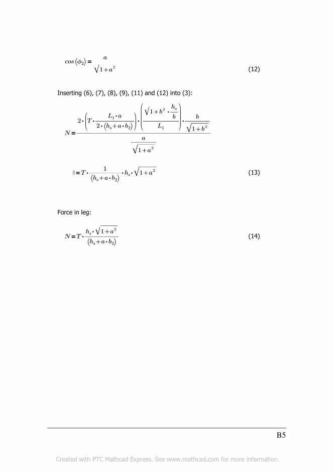
=cos ⎛⎝ϕ2⎞⎠ ―――a
‾‾‾‾‾+1 a2 (12)
Inserting (6), (7), (8), (9), (11) and (12) into (3):
=N ―――――――――――――――
⋅⋅⋅2⎛⎜⎝⋅T ―――――
⋅L1 a
⋅2 ⎛⎝ +hs ⋅a b2⎞⎠
⎞⎟⎠
⎛⎜⎜⎜⎝――――
⋅‾‾‾‾‾+1 b2 ―hs
b
L1
⎞⎟⎟⎟⎠―――
b
‾‾‾‾‾+1 b2
―――a
‾‾‾‾‾+1 a2
= ⋅⋅⋅T ――――1
⎛⎝ +hs ⋅a b2⎞⎠hs
‾‾‾‾‾+1 a2
Force in leg:
=N ⋅T ――――⋅hs
‾‾‾‾‾+1 a2
⎛⎝ +hs ⋅a b2⎞⎠
(13)
(14)
B5
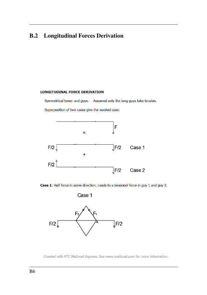
B.2 Longitudinal Forces Derivation
B6
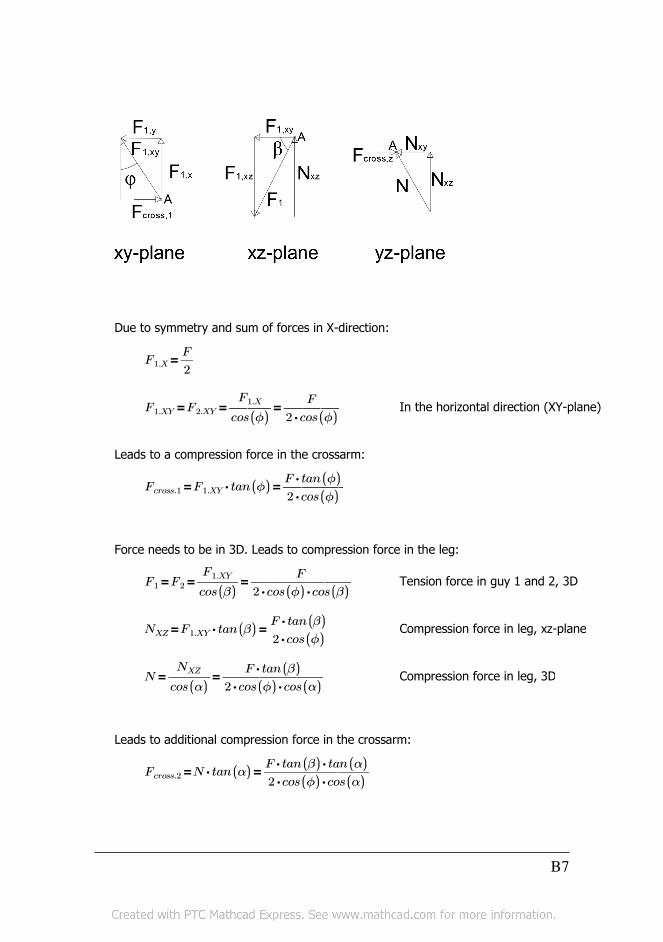
Due to symmetry and sum of forces in X-direction:
=F1.X ―F
2
===F1.XY F2.XY ―――F1.X
cos ((ϕ))――――
F
⋅2 cos ((ϕ))In the horizontal direction (XY-plane)
Leads to a compression force in the crossarm:
==Fcross.1 ⋅F1.XY tan ((ϕ)) ――――⋅F tan ((ϕ))
⋅2 cos ((ϕ))
Force needs to be in 3D. Leads to compression force in the leg:
===F1 F2 ―――F1.XY
cos ((β))――――――
F
⋅⋅2 cos ((ϕ)) cos ((β))Tension force in guy 1 and 2, 3D
==NXZ ⋅F1.XY tan ((β)) ――――⋅F tan ((β))
⋅2 cos ((ϕ))Compression force in leg, xz-plane
==N ―――NXZ
cos ((α))――――――
⋅F tan ((β))
⋅⋅2 cos ((ϕ)) cos ((α))Compression force in leg, 3D
Leads to additional compression force in the crossarm:
==Fcross.2 ⋅N tan ((α)) ――――――⋅⋅F tan ((β)) tan ((α))
⋅⋅2 cos ((ϕ)) cos ((α))
B7
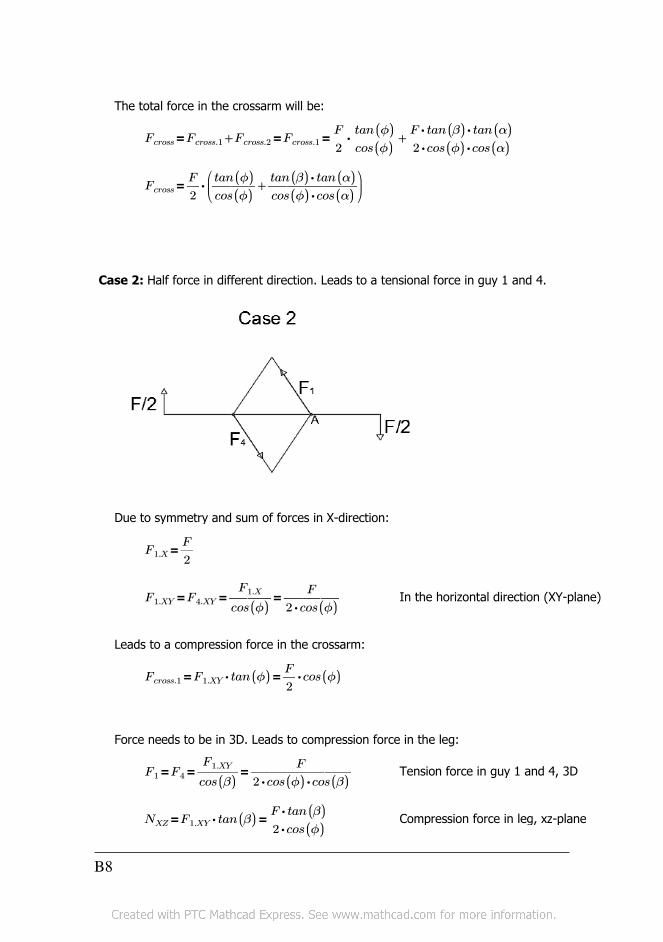
The total force in the crossarm will be:
===Fcross +Fcross.1 Fcross.2 Fcross.1 +⋅―F
2―――tan ((ϕ))
cos ((ϕ))――――――
⋅⋅F tan ((β)) tan ((α))
⋅⋅2 cos ((ϕ)) cos ((α))
=Fcross ⋅―F
2
⎛⎜⎝
+―――tan ((ϕ))
cos ((ϕ))―――――
⋅tan ((β)) tan ((α))
⋅cos ((ϕ)) cos ((α))
⎞⎟⎠
Case 2: Half force in different direction. Leads to a tensional force in guy 1 and 4.
Due to symmetry and sum of forces in X-direction:
=F1.X ―F
2
===F1.XY F4.XY ―――F1.X
cos ((ϕ))――――
F
⋅2 cos ((ϕ))In the horizontal direction (XY-plane)
Leads to a compression force in the crossarm:
==Fcross.1 ⋅F1.XY tan ((ϕ)) ⋅―F
2cos ((ϕ))
Force needs to be in 3D. Leads to compression force in the leg:
===F1 F4 ―――F1.XY
cos ((β))――――――
F
⋅⋅2 cos ((ϕ)) cos ((β))Tension force in guy 1 and 4, 3D
==NXZ ⋅F1.XY tan ((β)) ――――⋅F tan ((β))
⋅2 cos ((ϕ))Compression force in leg, xz-plane
B8
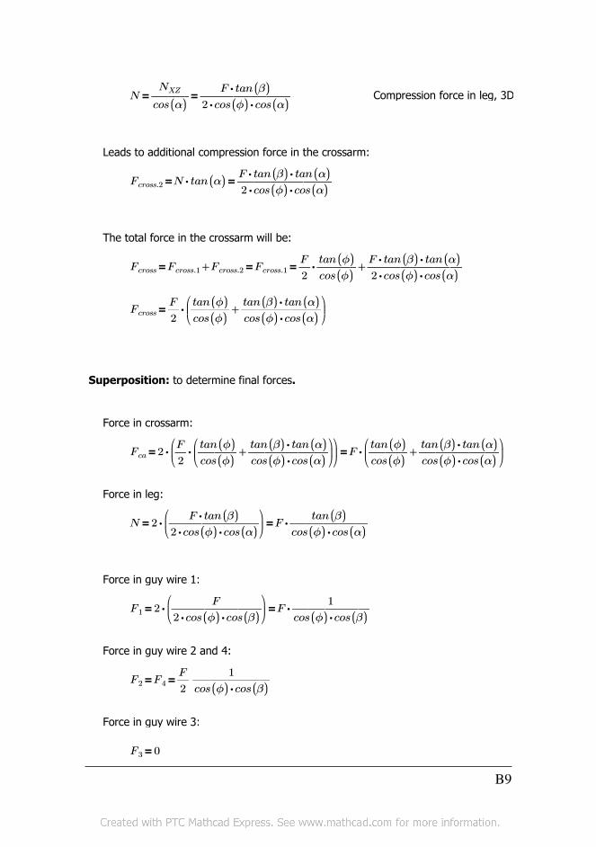
==N ―――NXZ
cos ((α))――――――
⋅F tan ((β))
⋅⋅2 cos ((ϕ)) cos ((α))Compression force in leg, 3D
Leads to additional compression force in the crossarm:
==Fcross.2 ⋅N tan ((α)) ――――――⋅⋅F tan ((β)) tan ((α))
⋅⋅2 cos ((ϕ)) cos ((α))
The total force in the crossarm will be:
===Fcross +Fcross.1 Fcross.2 Fcross.1 +⋅―F
2―――tan ((ϕ))
cos ((ϕ))――――――
⋅⋅F tan ((β)) tan ((α))
⋅⋅2 cos ((ϕ)) cos ((α))
=Fcross ⋅―F
2
⎛⎜⎝
+―――tan ((ϕ))
cos ((ϕ))―――――
⋅tan ((β)) tan ((α))
⋅cos ((ϕ)) cos ((α))
⎞⎟⎠
Superposition: to determine final forces.
Force in crossarm:
==Fca ⋅2⎛⎜⎝
⋅―F
2
⎛⎜⎝
+―――tan ((ϕ))
cos ((ϕ))―――――
⋅tan ((β)) tan ((α))
⋅cos ((ϕ)) cos ((α))
⎞⎟⎠
⎞⎟⎠
⋅F⎛⎜⎝
+―――tan ((ϕ))
cos ((ϕ))―――――
⋅tan ((β)) tan ((α))
⋅cos ((ϕ)) cos ((α))
⎞⎟⎠
Force in leg:
==N ⋅2⎛⎜⎝――――――
⋅F tan ((β))
⋅⋅2 cos ((ϕ)) cos ((α))
⎞⎟⎠
⋅F ―――――tan ((β))
⋅cos ((ϕ)) cos ((α))
Force in guy wire 1:
==F1 ⋅2⎛⎜⎝――――――
F
⋅⋅2 cos ((ϕ)) cos ((β))
⎞⎟⎠
⋅F ―――――1
⋅cos ((ϕ)) cos ((β))
Force in guy wire 2 and 4:
==F2 F4 ―F
2―――――
1
⋅cos ((ϕ)) cos ((β))
Force in guy wire 3:
=F3 0
B9
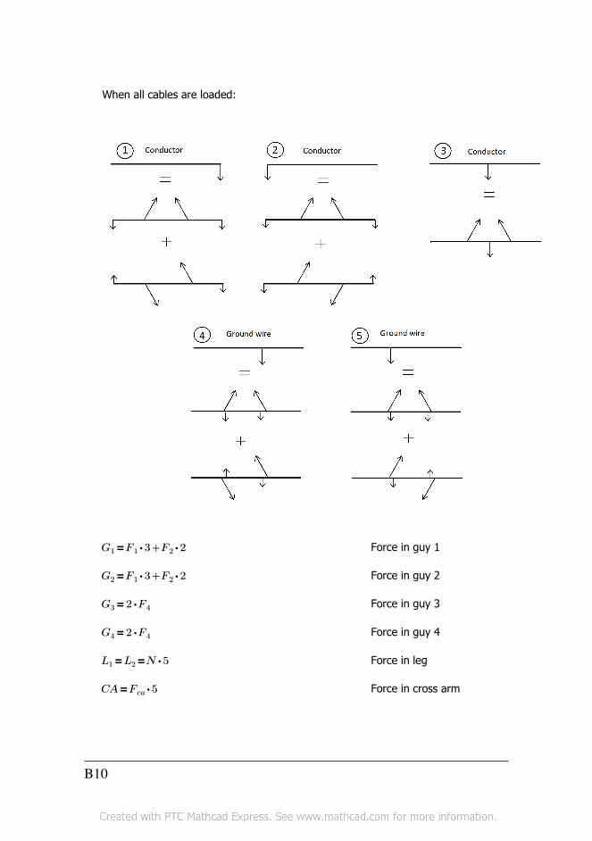
When all cables are loaded:
=G1 +⋅F1 3 ⋅F2 2 Force in guy 1
=G2 +⋅F1 3 ⋅F2 2 Force in guy 2
=G3 ⋅2 F4 Force in guy 3
=G4 ⋅2 F4 Force in guy 4
==L1 L2 ⋅N 5 Force in leg
=CA ⋅Fca 5 Force in cross arm
B10
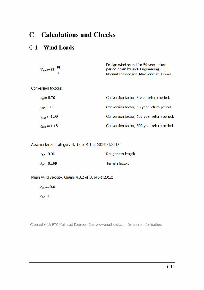
C Calculations and Checks
C.1 Wind Loads
C11
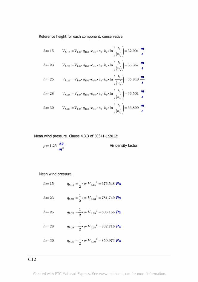
Reference height for each component, conservative.
≔h 15 ≔Vh.15 =⋅⋅⋅⋅⋅Vb.0 q150 cdir c0 kr ln⎛⎜⎝――h
⎛⎝z0⎞⎠
⎞⎟⎠
32.901 ―mmmm
ssss
≔h 23 ≔Vh.23 =⋅⋅⋅⋅⋅Vb.0 q150 cdir c0 kr ln⎛⎜⎝――h
⎛⎝z0⎞⎠
⎞⎟⎠
35.367 ―mmmm
ssss
≔h 25 ≔Vh.25 =⋅⋅⋅⋅⋅Vb.0 q150 cdir c0 kr ln⎛⎜⎝――h
⎛⎝z0⎞⎠
⎞⎟⎠
35.848 ―mmmm
ssss
≔h 28 ≔Vh.28 =⋅⋅⋅⋅⋅Vb.0 q150 cdir c0 kr ln⎛⎜⎝――h
⎛⎝z0⎞⎠
⎞⎟⎠
36.501 ―mmmm
ssss
≔h 30 ≔Vh.30 =⋅⋅⋅⋅⋅Vb.0 q150 cdir c0 kr ln⎛⎜⎝――h
⎛⎝z0⎞⎠
⎞⎟⎠
36.899 ―mmmm
ssss
Mean wind pressure. Clause 4.3.3 of 50341-1:2012:
≔ρ 1.25 ――kgkgkgkg
mmmm3
Air density factor.
Mean wind pressure.
≔h 15 ≔qh.15 =⋅⋅―1
2ρ Vh.15
2 676.548 PaPaPaPa
≔h 23 ≔qh.23 =⋅⋅―1
2ρ Vh.23
2 781.749 PaPaPaPa
≔h 25 ≔qh.25 =⋅⋅―1
2ρ Vh.25
2 803.156 PaPaPaPa
≔h 28 ≔qh.28 =⋅⋅―1
2ρ Vh.28
2 832.716 PaPaPaPa
≔h 30 ≔qh.30 =⋅⋅―1
2ρ Vh.30
2 850.973 PaPaPaPa
C12
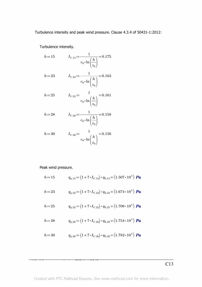
Turbulence intensity and peak wind pressure. Clause 4.3.4 of 50431-1:2012:
Turbulence intensity.
≔h 15 ≔IV.15 =――――1
⋅c0 ln⎛⎜⎝―h
z0
⎞⎟⎠
0.175
≔h 23 ≔IV.23 =――――1
⋅c0 ln⎛⎜⎝―h
z0
⎞⎟⎠
0.163
≔h 25 ≔IV.25 =――――1
⋅c0 ln⎛⎜⎝―h
z0
⎞⎟⎠
0.161
≔h 28 ≔IV.28 =――――1
⋅c0 ln⎛⎜⎝―h
z0
⎞⎟⎠
0.158
≔h 30 ≔IV.30 =――――1
⋅c0 ln⎛⎜⎝―h
z0
⎞⎟⎠
0.156
Peak wind pressure.
≔h 15 ≔qp.15 =⋅⎛⎝ +1 ⋅7 IV.15⎞⎠ qh.15⎛⎝ ⋅1.507 103 ⎞⎠ PaPaPaPa
≔h 23 ≔qp.23 =⋅⎛⎝ +1 ⋅7 IV.23⎞⎠ qh.23⎛⎝ ⋅1.674 103 ⎞⎠ PaPaPaPa
≔h 25 ≔qp.25 =⋅⎛⎝ +1 ⋅7 IV.25⎞⎠ qh.25⎛⎝ ⋅1.708 103 ⎞⎠ PaPaPaPa
≔h 28 ≔qp.28 =⋅⎛⎝ +1 ⋅7 IV.28⎞⎠ qh.28⎛⎝ ⋅1.754 103 ⎞⎠ PaPaPaPa
≔h 30 ≔qp.30 =⋅⎛⎝ +1 ⋅7 IV.30⎞⎠ qh.30⎛⎝ ⋅1.782 103 ⎞⎠ PaPaPaPa
Wind force on conductor, 50341 1:2012: C13

Wind force on conductor, 50341-1:2012:
=qp.23⎛⎝ ⋅1.674 103 ⎞⎠ PaPaPaPa Peak wind pressure
≔Gc 0.4 Structural factor for the conductor/span factor
N
≔Cc 1 Drag factor for the conductor/force coefficient
≔d ⋅34 3 mmmmmmmm Diameter of conductor
≔L1 350 mmmm Length of span 1
≔L2 350 mmmm Length of span 2
≔ϕ 0 degdegdegdeg Angle between wind direction and long. axis of crossarm
≔θ1 0 Change in angle of line
≔θ2 0 Change in angle of line
Wind coming in the direction of the crossarm:
≔Qwc.v1 =⋅⋅⋅⋅⋅qp.23 Gc Cc d cos ((ϕ))2
―――+L1 L2
223.909 kNkNkNkN
≔Qwc.v2 =0 0 ⋅―1
NNNNkNkNkNkN
Wind force on ground wire:
≔dgw 21 mmmmmmmm Diameter of conductor
≔Qgw =⋅⋅⋅⋅⋅qp.30 Gc Cc dgw cos ((ϕ))2
―――+L1 L2
25.24 kNkNkNkN
3 triplex conductors and two ground wires.
≔QT.c =⋅Qwc.v1 3 71.726 kNkNkNkN Wind force from all subconductors
≔QT.gw =⋅Qgw 2 10.479 kNkNkNkN Wind force from all subconductors
C14
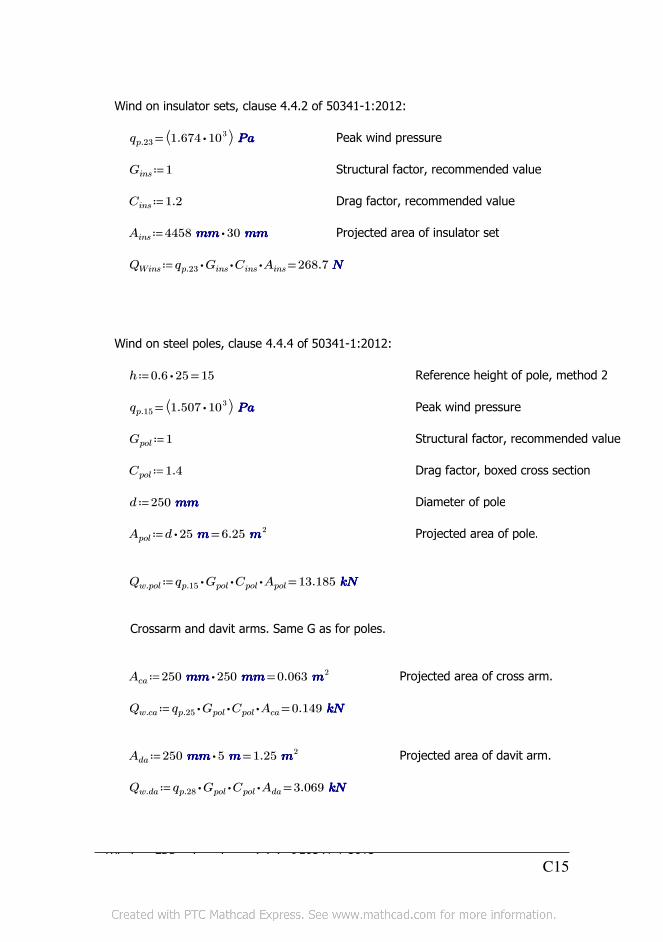
Wind on insulator sets, clause 4.4.2 of 50341-1:2012:
=qp.23⎛⎝ ⋅1.674 103 ⎞⎠ PaPaPaPa Peak wind pressure
≔Gins 1 Structural factor, recommended value
≔Cins 1.2 Drag factor, recommended value
≔Ains ⋅4458 mmmmmmmm 30 mmmmmmmm Projected area of insulator set
≔QWins =⋅⋅⋅qp.23 Gins Cins Ains 268.7 NNNN
Wind on steel poles, clause 4.4.4 of 50341-1:2012:
≔h =⋅0.6 25 15 Reference height of pole, method 2
=qp.15⎛⎝ ⋅1.507 103 ⎞⎠ PaPaPaPa Peak wind pressure
≔Gpol 1 Structural factor, recommended value
≔Cpol 1.4 Drag factor, boxed cross section
≔d 250 mmmmmmmm Diameter of pole
≔Apol =⋅d 25 mmmm 6.25 mmmm2 Projected area of pole.
≔Qw.pol =⋅⋅⋅qp.15 Gpol Cpol Apol 13.185 kNkNkNkN
Crossarm and davit arms. Same G as for poles.
≔Aca =⋅250 mmmmmmmm 250 mmmmmmmm 0.063 mmmm2 Projected area of cross arm.
≔Qw.ca =⋅⋅⋅qp.25 Gpol Cpol Aca 0.149 kNkNkNkN
≔Ada =⋅250 mmmmmmmm 5 mmmm 1.25 mmmm2 Projected area of davit arm.
≔Qw.da =⋅⋅⋅qp.28 Gpol Cpol Ada 3.069 kNkNkNkN
Wind on FRP poles, clause 4.4.4 of 50341 1:2012: C15
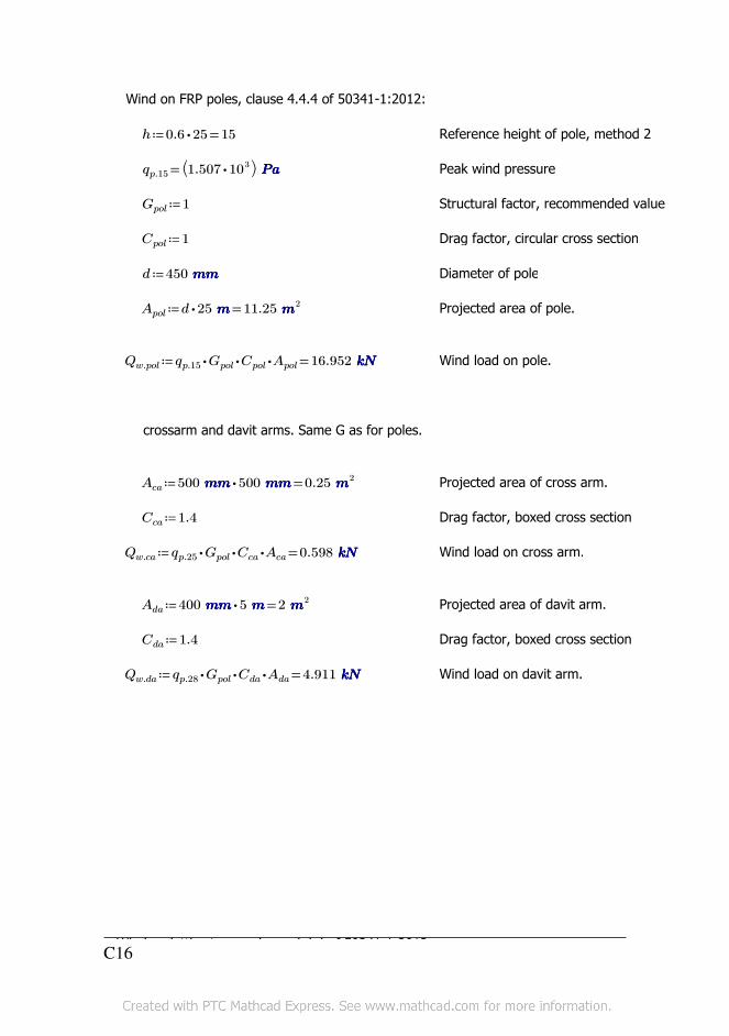
Wind on FRP poles, clause 4.4.4 of 50341-1:2012:
≔h =⋅0.6 25 15 Reference height of pole, method 2
=qp.15⎛⎝ ⋅1.507 103 ⎞⎠ PaPaPaPa Peak wind pressure
≔Gpol 1 Structural factor, recommended value
≔Cpol 1 Drag factor, circular cross section
≔d 450 mmmmmmmm Diameter of pole
≔Apol =⋅d 25 mmmm 11.25 mmmm2 Projected area of pole.
≔Qw.pol =⋅⋅⋅qp.15 Gpol Cpol Apol 16.952 kNkNkNkN Wind load on pole.
crossarm and davit arms. Same G as for poles.
≔Aca =⋅500 mmmmmmmm 500 mmmmmmmm 0.25 mmmm2 Projected area of cross arm.
≔Cca 1.4 Drag factor, boxed cross section
≔Qw.ca =⋅⋅⋅qp.25 Gpol Cca Aca 0.598 kNkNkNkN Wind load on cross arm.
≔Ada =⋅400 mmmmmmmm 5 mmmm 2 mmmm2 Projected area of davit arm.
≔Cda 1.4 Drag factor, boxed cross section
≔Qw.da =⋅⋅⋅qp.28 Gpol Cda Ada 4.911 kNkNkNkN Wind load on davit arm.
Wind on lattice tower, clause 4.4.4 of 50341 1:2012:C16
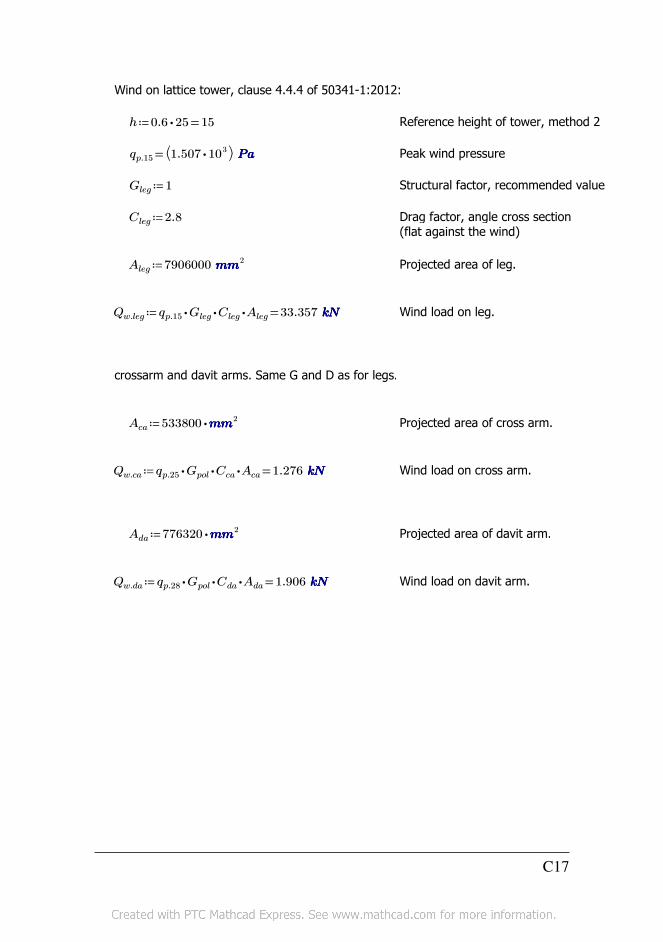
Wind on lattice tower, clause 4.4.4 of 50341-1:2012:
≔h =⋅0.6 25 15 Reference height of tower, method 2
=qp.15⎛⎝ ⋅1.507 103 ⎞⎠ PaPaPaPa Peak wind pressure
≔Gleg 1 Structural factor, recommended value
≔Cleg 2.8 Drag factor, angle cross section (flat against the wind)
≔Aleg 7906000 mmmmmmmm2 Projected area of leg.
≔Qw.leg =⋅⋅⋅qp.15 Gleg Cleg Aleg 33.357 kNkNkNkN Wind load on leg.
crossarm and davit arms. Same G and D as for legs.
≔Aca ⋅533800 mmmmmmmm2 Projected area of cross arm.
≔Qw.ca =⋅⋅⋅qp.25 Gpol Cca Aca 1.276 kNkNkNkN Wind load on cross arm.
≔Ada ⋅776320 mmmmmmmm2 Projected area of davit arm.
≔Qw.da =⋅⋅⋅qp.28 Gpol Cda Ada 1.906 kNkNkNkN Wind load on davit arm.
C17
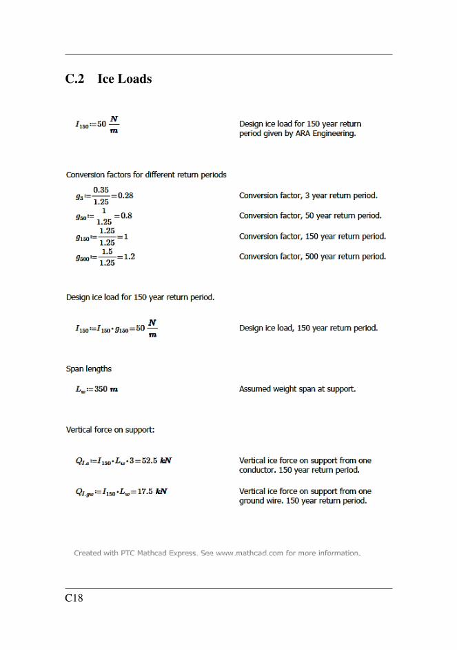
C.2 Ice Loads
C18
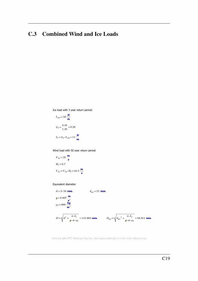
C.3 Combined Wind and Ice Loads
Ice load with 3 year return period:
≔I150 50 ―NNNN
mmmm
≔ψ3 =――0.35
1.250.28
≔I3 =⋅ψ3 I150 14 ―NNNN
mmmm
Wind load with 50 year return period:
≔V50 35 ―mmmm
ssss
≔BI 0.7
≔VIL =⋅V50 BI 24.5 ―mmmm
ssss
Equivalent diameter:
≔d ⋅3 34 mmmmmmmm ≔dgw 21 mmmmmmmm
=gggg 9.807 ―mmmm
ssss2
≔ρI 600 ――kgkgkgkg
mmmm3
≔D =‾‾‾‾‾‾‾‾‾‾
+d2 ―――⋅4 I3
⋅⋅gggg ππππ ρI115.903 mmmmmmmm ≔Dgw =
‾‾‾‾‾‾‾‾‾‾‾‾+dgw
2 ―――⋅4 I3
⋅⋅gggg ππππ ρI58.911 mmmmmmmm
C19
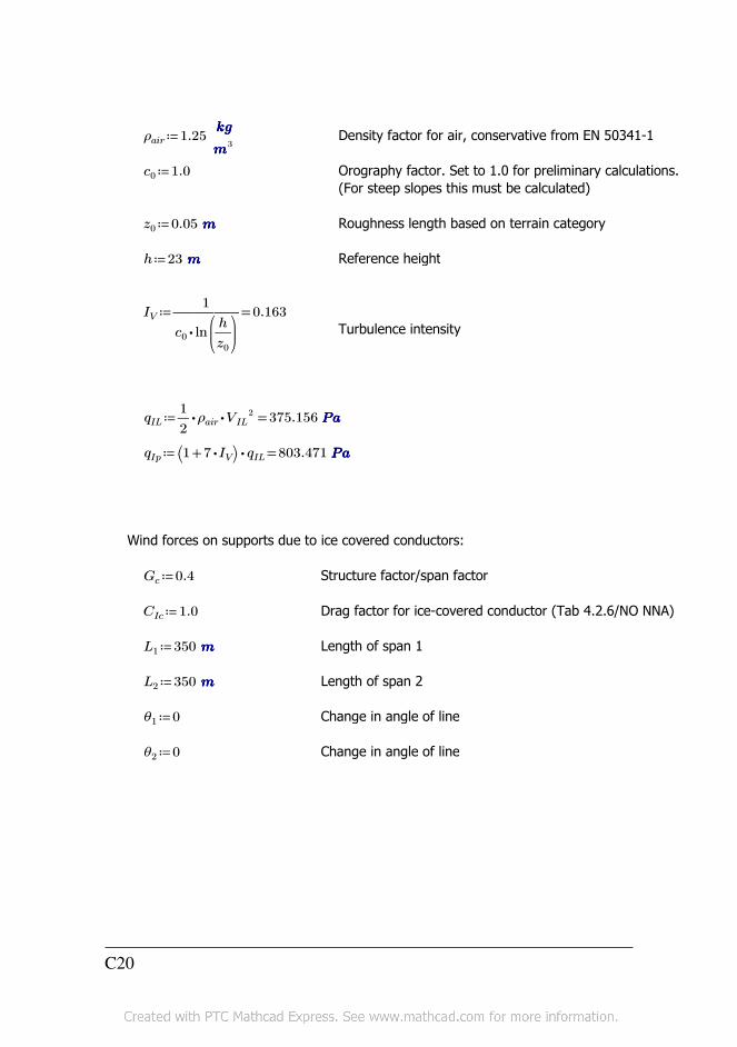
≔ρair 1.25 ――kgkgkgkg
mmmm3
Density factor for air, conservative from EN 50341-1
≔c0 1.0 Orography factor. Set to 1.0 for preliminary calculations.
(For steep slopes this must be calculated)
≔z0 0.05 mmmm Roughness length based on terrain category
≔h 23 mmmm Reference height
≔IV =――――1
⋅c0 ln⎛⎜⎝―h
z0
⎞⎟⎠
0.163Turbulence intensity
≔qIL =⋅⋅―1
2ρair VIL
2 375.156 PaPaPaPa
≔qIp =⋅⎛⎝ +1 ⋅7 IV⎞⎠ qIL 803.471 PaPaPaPa
Wind forces on supports due to ice covered conductors:
≔Gc 0.4 Structure factor/span factor
≔CIc 1.0 Drag factor for ice-covered conductor (Tab 4.2.6/NO NNA)
≔L1 350 mmmm Length of span 1
≔L2 350 mmmm Length of span 2
≔θ1 0 Change in angle of line
≔θ2 0 Change in angle of line
C20
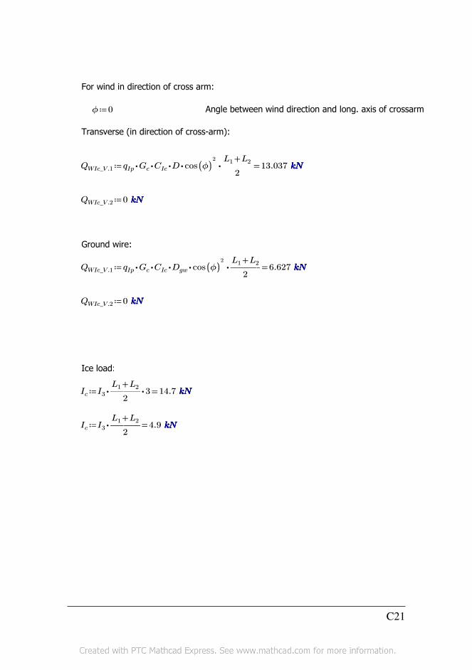
For wind in direction of cross arm:
≔ϕ 0 Angle between wind direction and long. axis of crossarm
Transverse (in direction of cross-arm):
≔QWIc_V.1 =⋅⋅⋅⋅⋅qIp Gc CIc D cos ((ϕ))2
―――+L1 L2
213.037 kNkNkNkN
≔QWIc_V.2 0 kNkNkNkN
Ground wire:
≔QWIc_V.1 =⋅⋅⋅⋅⋅qIp Gc CIc Dgw cos((ϕ))2
―――+L1 L2
26.627 kNkNkNkN
≔QWIc_V.2 0 kNkNkNkN
Ice load:
≔Ic =⋅⋅I3 ―――+L1 L2
23 14.7 kNkNkNkN
≔Ic =⋅I3 ―――+L1 L2
24.9 kNkNkNkN
C21
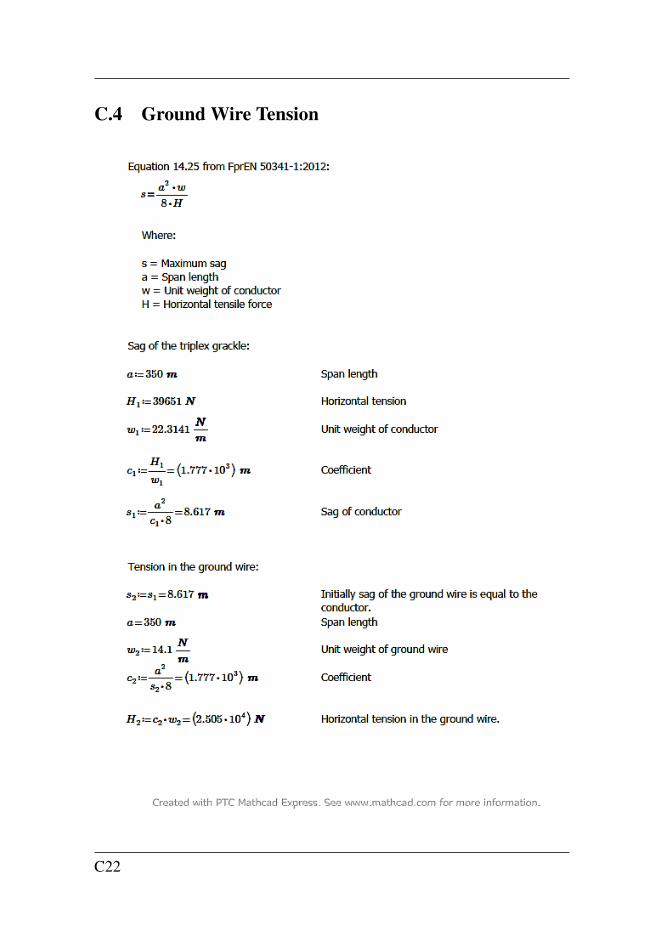
C.4 Ground Wire Tension
C22
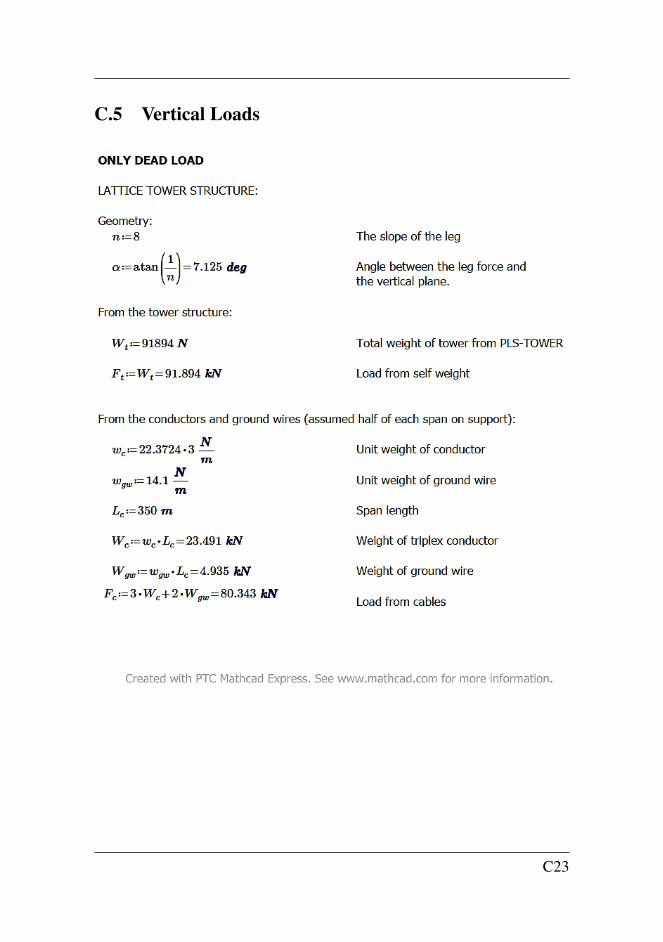
C.5 Vertical Loads
C23
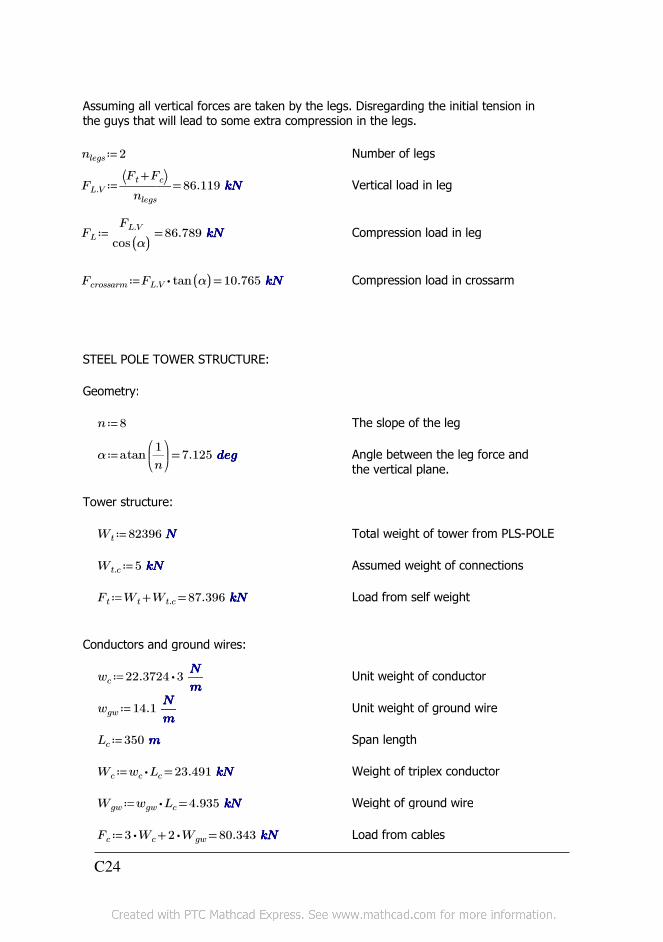
Assuming all vertical forces are taken by the legs. Disregarding the initial tension in the guys that will lead to some extra compression in the legs.
≔nlegs 2 Number of legs
≔FL.V =―――⎛⎝ +Ft Fc⎞⎠
nlegs86.119 kNkNkNkN Vertical load in leg
≔FL =―――FL.V
cos ((α))86.789 kNkNkNkN Compression load in leg
≔Fcrossarm =⋅FL.V tan((α)) 10.765 kNkNkNkN Compression load in crossarm
STEEL POLE TOWER STRUCTURE:
Geometry:
≔n 8 The slope of the leg
≔α =atan⎛⎜⎝―1
n
⎞⎟⎠
7.125 degdegdegdeg Angle between the leg force and the vertical plane.
Tower structure:
≔Wt 82396 NNNN Total weight of tower from PLS-POLE
≔Wt.c 5 kNkNkNkN Assumed weight of connections
≔Ft =+Wt Wt.c 87.396 kNkNkNkN Load from self weight
Conductors and ground wires:
≔wc ⋅22.3724 3 ―NNNN
mmmmUnit weight of conductor
≔wgw 14.1 ―NNNN
mmmmUnit weight of ground wire
≔Lc 350 mmmm Span length
≔Wc =⋅wc Lc 23.491 kNkNkNkN Weight of triplex conductor
≔Wgw =⋅wgw Lc 4.935 kNkNkNkN Weight of ground wire
≔Fc =+⋅3 Wc ⋅2 Wgw 80.343 kNkNkNkN Load from cables
C24
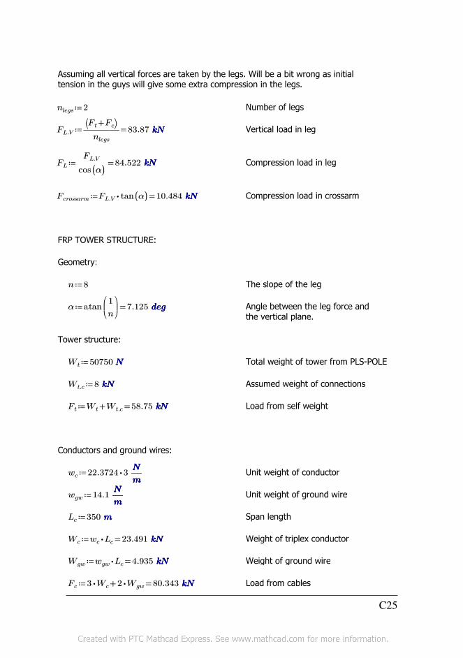
Assuming all vertical forces are taken by the legs. Will be a bit wrong as initial tension in the guys will give some extra compression in the legs.
≔nlegs 2 Number of legs
≔FL.V =―――⎛⎝ +Ft Fc⎞⎠
nlegs83.87 kNkNkNkN Vertical load in leg
≔FL =―――FL.V
cos ((α))84.522 kNkNkNkN Compression load in leg
≔Fcrossarm =⋅FL.V tan((α)) 10.484 kNkNkNkN Compression load in crossarm
FRP TOWER STRUCTURE:
Geometry:
≔n 8 The slope of the leg
≔α =atan⎛⎜⎝―1
n
⎞⎟⎠
7.125 degdegdegdeg Angle between the leg force and the vertical plane.
Tower structure:
≔Wt 50750 NNNN Total weight of tower from PLS-POLE
≔Wt.c 8 kNkNkNkN Assumed weight of connections
≔Ft =+Wt Wt.c 58.75 kNkNkNkN Load from self weight
Conductors and ground wires:
≔wc ⋅22.3724 3 ―NNNN
mmmmUnit weight of conductor
≔wgw 14.1 ―NNNN
mmmmUnit weight of ground wire
≔Lc 350 mmmm Span length
≔Wc =⋅wc Lc 23.491 kNkNkNkN Weight of triplex conductor
≔Wgw =⋅wgw Lc 4.935 kNkNkNkN Weight of ground wire
≔Fc =+⋅3 Wc ⋅2 Wgw 80.343 kNkNkNkN Load from cables
C25
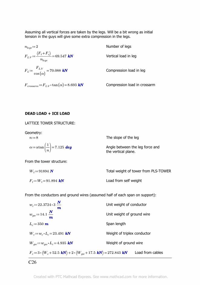
Assuming all vertical forces are taken by the legs. Will be a bit wrong as initial tension in the guys will give some extra compression in the legs.
≔nlegs 2 Number of legs
≔FL.V =―――⎛⎝ +Ft Fc⎞⎠
nlegs69.547 kNkNkNkN Vertical load in leg
≔FL =―――FL.V
cos ((α))70.088 kNkNkNkN Compression load in leg
≔Fcrossarm =⋅FL.V tan((α)) 8.693 kNkNkNkN Compression load in crossarm
DEAD LOAD + ICE LOAD
LATTICE TOWER STRUCTURE:
Geometry:
≔n 8 The slope of the leg
≔α =atan⎛⎜⎝―1
n
⎞⎟⎠
7.125 degdegdegdeg Angle between the leg force and the vertical plane.
From the tower structure:
≔Wt 91894 NNNN Total weight of tower from PLS-TOWER
≔Ft =Wt 91.894 kNkNkNkN Load from self weight
From the conductors and ground wires (assumed half of each span on support):
≔wc ⋅22.3724 3 ―NNNN
mmmmUnit weight of conductor
≔wgw 14.1 ―NNNN
mmmmUnit weight of ground wire
≔Lc 350 mmmm Span length
≔Wc =⋅wc Lc 23.491 kNkNkNkN Weight of triplex conductor
≔Wgw =⋅wgw Lc 4.935 kNkNkNkN Weight of ground wire
≔Fc =+⋅3 ⎛⎝ +Wc 52.5 kNkNkNkN⎞⎠ ⋅2 ⎛⎝ +Wgw 17.5 kNkNkNkN⎞⎠ 272.843 kNkNkNkN Load from cables
C26
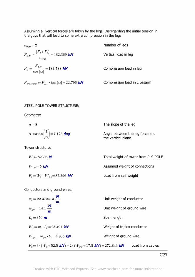
Assuming all vertical forces are taken by the legs. Disregarding the initial tension in the guys that will lead to some extra compression in the legs.
≔nlegs 2 Number of legs
≔FL.V =―――⎛⎝ +Ft Fc⎞⎠
nlegs182.369 kNkNkNkN Vertical load in leg
≔FL =―――FL.V
cos ((α))183.788 kNkNkNkN Compression load in leg
≔Fcrossarm =⋅FL.V tan((α)) 22.796 kNkNkNkN Compression load in crossarm
STEEL POLE TOWER STRUCTURE:
Geometry:
≔n 8 The slope of the leg
≔α =atan⎛⎜⎝―1
n
⎞⎟⎠
7.125 degdegdegdeg Angle between the leg force and the vertical plane.
Tower structure:
≔Wt 82396 NNNN Total weight of tower from PLS-POLE
≔Wt.c 5 kNkNkNkN Assumed weight of connections
≔Ft =+Wt Wt.c 87.396 kNkNkNkN Load from self weight
Conductors and ground wires:
≔wc ⋅22.3724 3 ―NNNN
mmmmUnit weight of conductor
≔wgw 14.1 ―NNNN
mmmmUnit weight of ground wire
≔Lc 350 mmmm Span length
≔Wc =⋅wc Lc 23.491 kNkNkNkN Weight of triplex conductor
≔Wgw =⋅wgw Lc 4.935 kNkNkNkN Weight of ground wire
≔Fc =+⋅3 ⎛⎝ +Wc 52.5 kNkNkNkN⎞⎠ ⋅2 ⎛⎝ +Wgw 17.5 kNkNkNkN⎞⎠ 272.843 kNkNkNkN Load from cables
C27
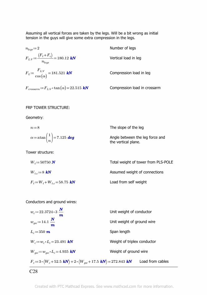
Assuming all vertical forces are taken by the legs. Will be a bit wrong as initial tension in the guys will give some extra compression in the legs.
≔nlegs 2 Number of legs
≔FL.V =―――⎛⎝ +Ft Fc⎞⎠
nlegs180.12 kNkNkNkN Vertical load in leg
≔FL =―――FL.V
cos ((α))181.521 kNkNkNkN Compression load in leg
≔Fcrossarm =⋅FL.V tan((α)) 22.515 kNkNkNkN Compression load in crossarm
FRP TOWER STRUCTURE:
Geometry:
≔n 8 The slope of the leg
≔α =atan⎛⎜⎝―1
n
⎞⎟⎠
7.125 degdegdegdeg Angle between the leg force and the vertical plane.
Tower structure:
≔Wt 50750 NNNN Total weight of tower from PLS-POLE
≔Wt.c 8 kNkNkNkN Assumed weight of connections
≔Ft =+Wt Wt.c 58.75 kNkNkNkN Load from self weight
Conductors and ground wires:
≔wc ⋅22.3724 3 ―NNNN
mmmmUnit weight of conductor
≔wgw 14.1 ―NNNN
mmmmUnit weight of ground wire
≔Lc 350 mmmm Span length
≔Wc =⋅wc Lc 23.491 kNkNkNkN Weight of triplex conductor
≔Wgw =⋅wgw Lc 4.935 kNkNkNkN Weight of ground wire
≔Fc =+⋅3 ⎛⎝ +Wc 52.5 kNkNkNkN⎞⎠ ⋅2 ⎛⎝ +Wgw 17.5 kNkNkNkN⎞⎠ 272.843 kNkNkNkN Load from cables
C28

Assuming all vertical forces are taken by the legs. Will be a bit wrong as initial tension in the guys will give some extra compression in the legs.
≔nlegs 2 Number of legs
≔FL.V =―――⎛⎝ +Ft Fc⎞⎠
nlegs165.797 kNkNkNkN Vertical load in leg
≔FL =―――FL.V
cos ((α))167.087 kNkNkNkN Compression load in leg
≔Fcrossarm =⋅FL.V tan((α)) 20.725 kNkNkNkN Compression load in crossarm
C29
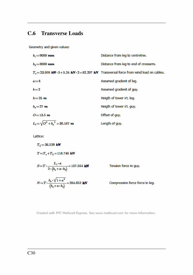
C.6 Transverse Loads
C30
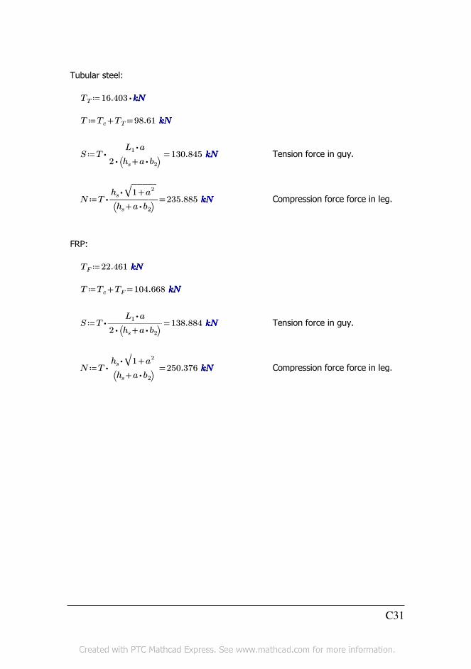
Tubular steel:
≔TT ⋅16.403 kNkNkNkN
≔T =+Tc TT 98.61 kNkNkNkN
≔S =⋅T ―――――⋅L1 a
⋅2 ⎛⎝ +hs ⋅a b2⎞⎠130.845 kNkNkNkN Tension force in guy.
≔N =⋅T ――――⋅hs‾‾‾‾‾+1 a
2
⎛⎝ +hs ⋅a b2⎞⎠235.885 kNkNkNkN Compression force force in leg.
FRP:
≔TF 22.461 kNkNkNkN
≔T =+Tc TF 104.668 kNkNkNkN
≔S =⋅T ―――――⋅L1 a
⋅2 ⎛⎝ +hs ⋅a b2⎞⎠138.884 kNkNkNkN Tension force in guy.
≔N =⋅T ――――⋅hs‾‾‾‾‾+1 a
2
⎛⎝ +hs ⋅a b2⎞⎠250.376 kNkNkNkN Compression force force in leg.
C31
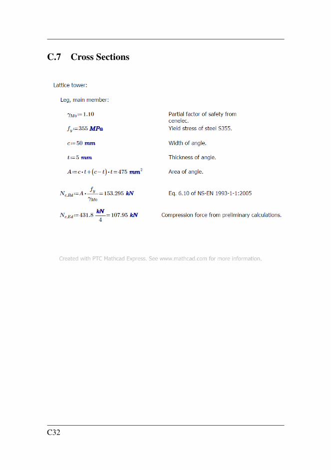
C.7 Cross Sections
C32
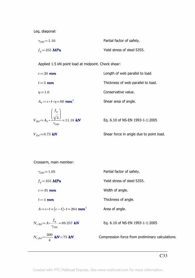
Leg, diagonal:
≔γM0 1.10 Partial factor of safety.
≔fy 355 MPaMPaMPaMPa Yield stress of steel S355.
Applied 1.5 kN point load at midpoint. Check shear:
≔c 20 mmmmmmmm Length of web parallel to load.
≔t 3 mmmmmmmm Thickness of web parallel to load.
≔η 1.0 Conservative value.
≔AV =⋅⋅c t η 60 mmmmmmmm2 Shear area of angle.
≔VRd =⋅AV ―――
⎛⎜⎜⎝――fy
‾‾3
⎞⎟⎟⎠
γM0
11.18 kNkNkNkN Eq. 6.10 of NS-EN 1993-1-1:2005
≔VEd 0.75 kNkNkNkN Shear force in angle due to point load.
Crossarm, main member:
≔γM0 1.05 Partial factor of safety.
≔fy 355 MPaMPaMPaMPa Yield stress of steel S355.
≔c 35 mmmmmmmm Width of angle.
≔t 4 mmmmmmmm Thickness of angle.
≔A =+⋅c t ⋅(( −c t)) t 264 mmmmmmmm2 Area of angle.
≔Nc.Rd =⋅A ――fy
γM0
89.257 kNkNkNkN Eq. 6.10 of NS-EN 1993-1-1:2005
≔Nc.Ed =――300
4kNkNkNkN 75 kNkNkNkN Compression force from preliminary calculations.
C33
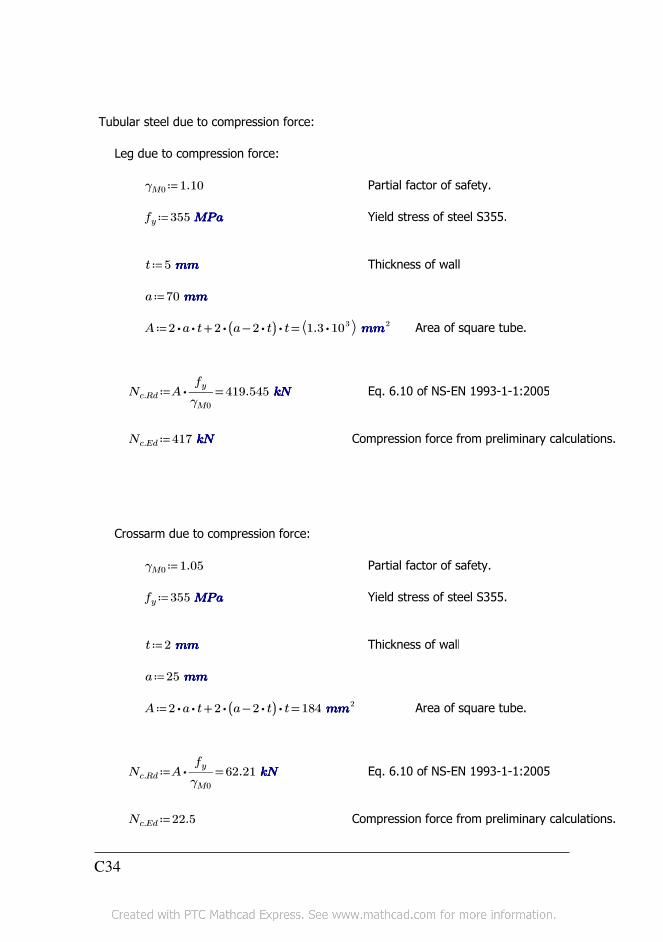
Tubular steel due to compression force:
Leg due to compression force:
≔γM0 1.10 Partial factor of safety.
≔fy 355 MPaMPaMPaMPa Yield stress of steel S355.
≔t 5 mmmmmmmm Thickness of wall
≔a 70 mmmmmmmm
≔A =+⋅⋅2 a t ⋅⋅2 (( −a ⋅2 t)) t ⎛⎝ ⋅1.3 103 ⎞⎠ mmmmmmmm2 Area of square tube.
≔Nc.Rd =⋅A ――fy
γM0
419.545 kNkNkNkN Eq. 6.10 of NS-EN 1993-1-1:2005
≔Nc.Ed 417 kNkNkNkN Compression force from preliminary calculations.
Crossarm due to compression force:
≔γM0 1.05 Partial factor of safety.
≔fy 355 MPaMPaMPaMPa Yield stress of steel S355.
≔t 2 mmmmmmmm Thickness of wall
≔a 25 mmmmmmmm
≔A =+⋅⋅2 a t ⋅⋅2 (( −a ⋅2 t)) t 184 mmmmmmmm2 Area of square tube.
≔Nc.Rd =⋅A ――fy
γM0
62.21 kNkNkNkN Eq. 6.10 of NS-EN 1993-1-1:2005
≔Nc.Ed 22.5 Compression force from preliminary calculations.
C34
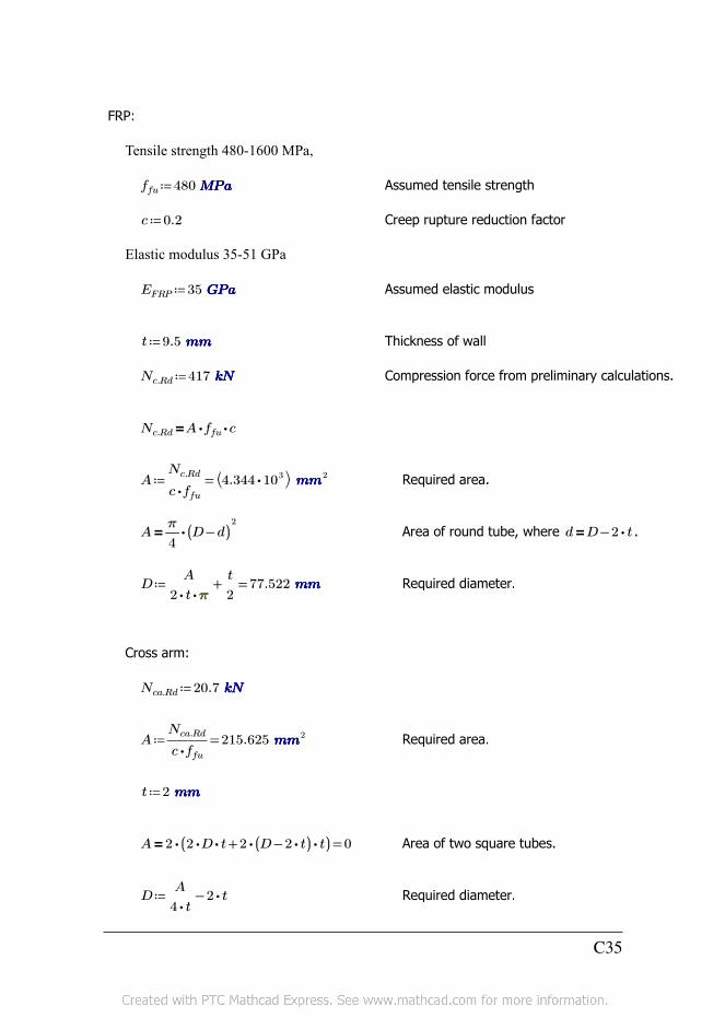
FRP:
Tensile strength 480-1600 MPa,
≔ffu 480 MPaMPaMPaMPa Assumed tensile strength
≔c 0.2 Creep rupture reduction factor
Elastic modulus 35-51 GPa
≔EFRP 35 GPaGPaGPaGPa Assumed elastic modulus
≔t 9.5 mmmmmmmm Thickness of wall
≔Nc.Rd 417 kNkNkNkN Compression force from preliminary calculations.
=Nc.Rd ⋅⋅A ffu c
≔A =――Nc.Rd
⋅c ffu
⎛⎝ ⋅4.344 103 ⎞⎠ mmmmmmmm2 Required area.
=A ⋅―π
4(( −D d))
2Area of round tube, where .=d −D ⋅2 t
≔D =+―――A
⋅⋅2 t ππππ―t
277.522 mmmmmmmm Required diameter.
Cross arm:
≔Nca.Rd 20.7 kNkNkNkN
≔A =―――Nca.Rd
⋅c ffu215.625 mmmmmmmm2 Required area.
≔t 2 mmmmmmmm
==A ⋅2 (( +⋅⋅2 D t ⋅⋅2 (( −D ⋅2 t)) t)) 0 Area of two square tubes.
≔D −――A
⋅4 t⋅2 t Required diameter.
C35
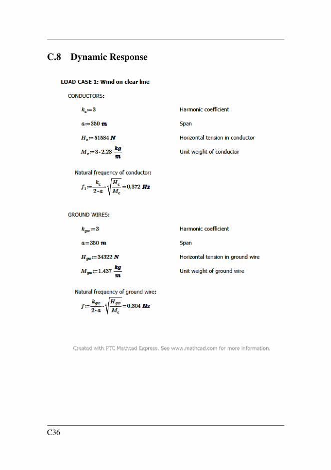
C.8 Dynamic Response
C36
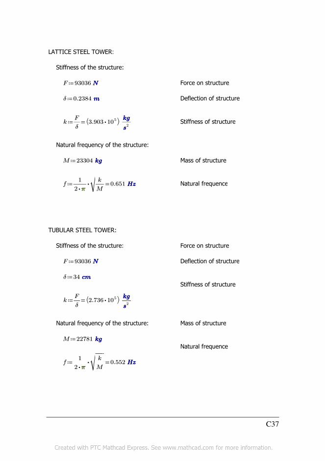
LATTICE STEEL TOWER:
Stiffness of the structure:
≔F 93036 NNNN Force on structure
≔δ 0.2384 mmmm Deflection of structure
≔k =―F
δ⎛⎝ ⋅3.903 105 ⎞⎠ ―
kgkgkgkg
ssss2
Stiffness of structure
Natural frequency of the structure:
≔M 23304 kgkgkgkg Mass of structure
≔f =⋅――1
⋅2 ππππ
‾‾‾―k
M0.651 HzHzHzHz Natural frequence
TUBULAR STEEL TOWER:
Stiffness of the structure: Force on structure
≔F 93036 NNNN Deflection of structure
≔δ 34 cmcmcmcmStiffness of structure
≔k =―F
δ⎛⎝ ⋅2.736 105 ⎞⎠ ―
kgkgkgkg
ssss2
Natural frequency of the structure: Mass of structure
≔M 22781 kgkgkgkgNatural frequence
≔f =⋅――1
⋅2 ππππ
‾‾‾―k
M0.552 HzHzHzHz
C37

TUBULAR FRP TOWER:
Stiffness of the structure:
Force on structure≔F 111841 NNNN
Deflection of structure≔δ 60.36 cmcmcmcm
Stiffness of structure≔k =―F
δ⎛⎝ ⋅1.853 105 ⎞⎠ ―
kgkgkgkg
ssss2
Natural frequency of the structure:
Mass of structure≔M 21108 kgkgkgkg
Natural frequence≔f =⋅――1
⋅2 ππππ
‾‾‾―k
M0.472 HzHzHzHz
LOAD CASE 2: Wind on iced line
CONDUCTORS:
≔kc 3 Harmonic coefficient
≔a 350 mmmm Span
≔Hc 40405 NNNN Horizontal tension in conductor
≔Mc ⋅3 2.28 ―kgkgkgkg
mmmmUnit weight of conductor
Natural frequency of conductor:
≔f1 =⋅――kc
⋅2 a
‾‾‾――Hc
Mc
0.329 HzHzHzHz
C38
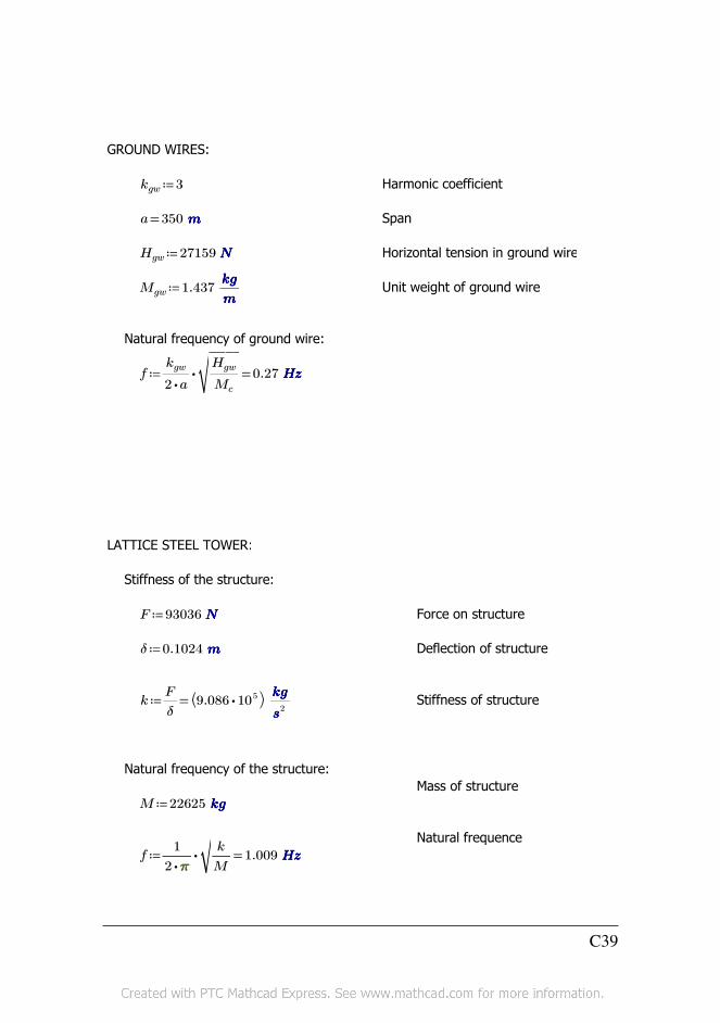
GROUND WIRES:
≔kgw 3 Harmonic coefficient
=a 350 mmmm Span
≔Hgw 27159 NNNN Horizontal tension in ground wire
≔Mgw 1.437 ―kgkgkgkg
mmmmUnit weight of ground wire
Natural frequency of ground wire:
≔f =⋅――kgw
⋅2 a
‾‾‾‾――Hgw
Mc
0.27 HzHzHzHz
LATTICE STEEL TOWER:
Stiffness of the structure:
≔F 93036 NNNN Force on structure
≔δ 0.1024 mmmm Deflection of structure
≔k =―F
δ⎛⎝ ⋅9.086 105 ⎞⎠ ―
kgkgkgkg
ssss2
Stiffness of structure
Natural frequency of the structure:
Mass of structure
≔M 22625 kgkgkgkg
Natural frequence
≔f =⋅――1
⋅2 ππππ
‾‾‾―k
M1.009 HzHzHzHz
C39
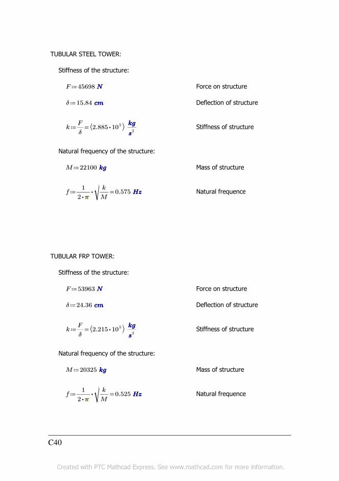
TUBULAR STEEL TOWER:
Stiffness of the structure:
≔F 45698 NNNN Force on structure
≔δ 15.84 cmcmcmcm Deflection of structure
≔k =―F
δ⎛⎝ ⋅2.885 105 ⎞⎠ ―
kgkgkgkg
ssss2
Stiffness of structure
Natural frequency of the structure:
≔M 22100 kgkgkgkg Mass of structure
≔f =⋅――1
⋅2 ππππ
‾‾‾―k
M0.575 HzHzHzHz Natural frequence
TUBULAR FRP TOWER:
Stiffness of the structure:
≔F 53963 NNNN Force on structure
≔δ 24.36 cmcmcmcm Deflection of structure
≔k =―F
δ⎛⎝ ⋅2.215 105 ⎞⎠ ―
kgkgkgkg
ssss2
Stiffness of structure
Natural frequency of the structure:
≔M 20325 kgkgkgkg Mass of structure
≔f =⋅――1
⋅2 ππππ
‾‾‾―k
M0.525 HzHzHzHz Natural frequence
C40
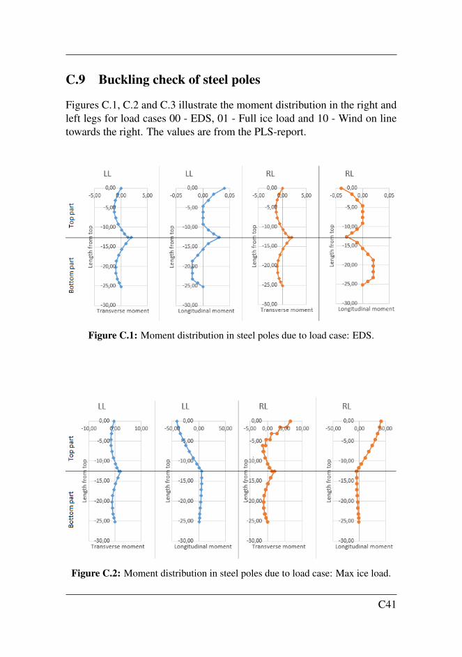
C.9 Buckling check of steel poles
Figures C.1, C.2 and C.3 illustrate the moment distribution in the right andleft legs for load cases 00 - EDS, 01 - Full ice load and 10 - Wind on linetowards the right. The values are from the PLS-report.
Figure C.1: Moment distribution in steel poles due to load case: EDS.
Figure C.2: Moment distribution in steel poles due to load case: Max ice load.
C41
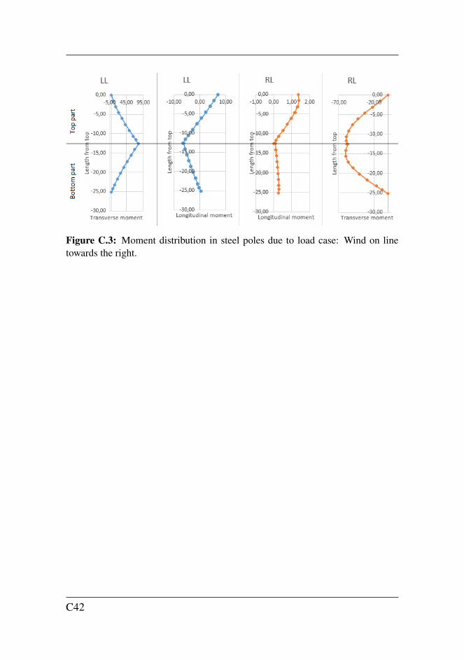
Figure C.3: Moment distribution in steel poles due to load case: Wind on linetowards the right.
C42
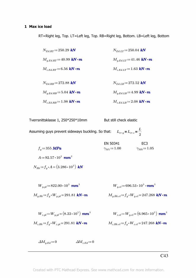
1 Max ice load
RT=Right leg, Top. LT=Left leg, Top. RB=Right leg, Bottom. LB=Left leg, Bottom
≔NEd.RT 250.29 kNkNkNkN ≔NEd.LT 250.04 kNkNkNkN
≔My.Ed.RT ⋅40.99 kNkNkNkN mmmm ≔My.Ed.LT ⋅41.46 kNkNkNkN mmmm
≔Mz.Ed.RT ⋅6.56 kNkNkNkN mmmm ≔Mz.Ed.LT ⋅1.63 kNkNkNkN mmmm
≔NEd.RB 272.88 kNkNkNkN ≔NEd.LB 272.52 kNkNkNkN
≔My.Ed.RB ⋅5.04 kNkNkNkN mmmm ≔My.Ed.LB ⋅4.99 kNkNkNkN mmmm
≔Mz.Ed.RB ⋅1.98 kNkNkNkN mmmm ≔Mz.Ed.LB ⋅2.08 kNkNkNkN mmmm
Tverrsnittsklasse 1, 250*250*10mm But still check elastic
Assuming guys prevent sideways buckling. So that: ==Lcr.y Lcr.z ―L
2
EN 50341 EC3
≔fy 355 MPaMPaMPaMPa ≔γM1 1.00 ≔γM0 1.05
≔A ⋅92.57 102 mmmmmmmm2
≔NRk =⋅fy A ⎛⎝ ⋅3.286 103 ⎞⎠ kNkNkNkN
≔Wy.pl ⋅822.00 103 mmmmmmmm3 ≔Wy.el ⋅⋅696.53 103 mmmmmmmm3
≔My.Rk =⋅fy Wy.pl 291.81 ⋅kNkNkNkN mmmm ≔My.Rk.el =⋅fy Wy.el 247.268 ⋅kNkNkNkN mmmm
≔Wz.pl =Wy.pl⎛⎝ ⋅8.22 105 ⎞⎠ mmmmmmmm3 ≔Wz.el =Wy.el
⎛⎝ ⋅6.965 105 ⎞⎠ mmmmmmmm3
≔Mz.Rk =⋅fy Wz.pl 291.81 ⋅kNkNkNkN mmmm ≔Mz.Rk.el =⋅fy Wz.el 247.268 ⋅kNkNkNkN mmmm
≔∆My.Ed 0 ≔∆Mz.Ed 0
C43
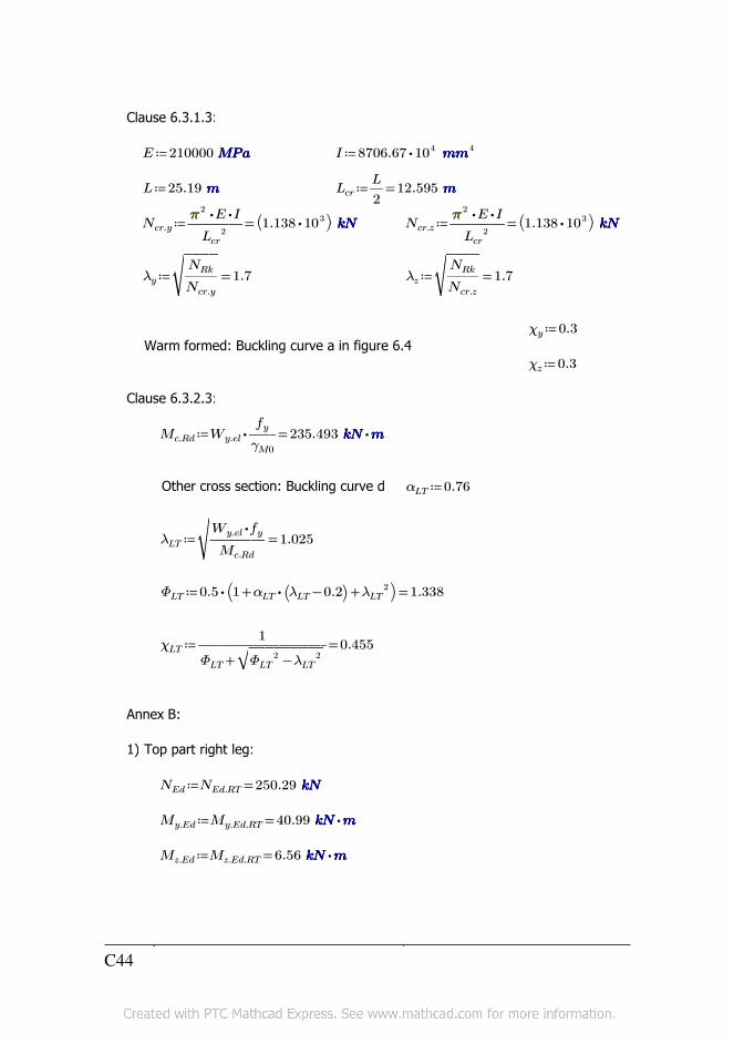
Clause 6.3.1.3:
≔E 210000 MPaMPaMPaMPa ≔I ⋅8706.67 104 mmmmmmmm4
≔L 25.19 mmmm ≔Lcr =―L
212.595 mmmm
≔Ncr.y =―――⋅⋅ππππ
2 E I
Lcr2
⎛⎝ ⋅1.138 103 ⎞⎠ kNkNkNkN ≔Ncr.z =―――⋅⋅ππππ
2 E I
Lcr2
⎛⎝ ⋅1.138 103 ⎞⎠ kNkNkNkN
≔λy =‾‾‾‾‾――NRk
Ncr.y
1.7 ≔λz =‾‾‾‾‾――NRk
Ncr.z
1.7
≔χy 0.3Warm formed: Buckling curve a in figure 6.4
≔χz 0.3
Clause 6.3.2.3:
≔Mc.Rd =⋅Wy.el ――fy
γM0
235.493 ⋅kNkNkNkN mmmm
Other cross section: Buckling curve d ≔αLT 0.76
≔λLT =‾‾‾‾‾‾‾―――
⋅Wy.el fy
Mc.Rd
1.025
≔ΦLT =⋅0.5 ⎛⎝ ++1 ⋅αLT ⎛⎝ −λLT 0.2⎞⎠ λLT2 ⎞⎠ 1.338
≔χLT =―――――――1
+ΦLT‾‾‾‾‾‾‾‾‾‾−ΦLT
2 λLT2
0.455
Annex B:
1) Top part right leg:
≔NEd =NEd.RT 250.29 kNkNkNkN
≔My.Ed =My.Ed.RT 40.99 ⋅kNkNkNkN mmmm
≔Mz.Ed =Mz.Ed.RT 6.56 ⋅kNkNkNkN mmmm
1 ψ 0.139Long.:C44
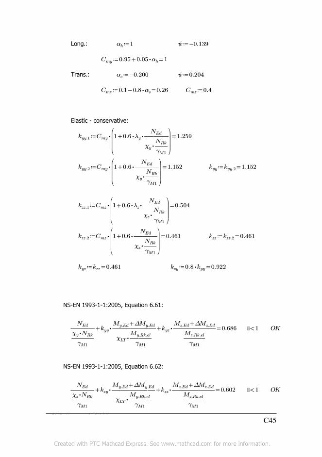
Long.: ≔αh 1 ≔ψ −0.139
≔Cmy =+0.95 ⋅0.05 αh 1
Trans.: ≔αs −0.200 ≔ψ 0.204
≔Cmz =−0.1 ⋅0.8 αs 0.26 ≔Cmz 0.4
Elastic - conservative:
≔kyy.1 =⋅Cmy
⎛⎜⎜⎜⎝
+1 ⋅⋅0.6 λy ―――NEd
⋅χy ――NRk
γM1
⎞⎟⎟⎟⎠
1.259
≔kyy.2 =⋅Cmy
⎛⎜⎜⎜⎝
+1 ⋅0.6 ―――NEd
⋅χy ――NRk
γM1
⎞⎟⎟⎟⎠
1.152 ≔kyy =kyy.2 1.152
≔kzz.1 =⋅Cmz
⎛⎜⎜⎜⎝
+1 ⋅⋅0.6 λz ―――NEd
⋅χz ――NRk
γM1
⎞⎟⎟⎟⎠
0.504
≔kzz.2 =⋅Cmz
⎛⎜⎜⎜⎝
+1 ⋅0.6 ―――NEd
⋅χz ――NRk
γM1
⎞⎟⎟⎟⎠
0.461 ≔kzz =kzz.2 0.461
≔kyz =kzz 0.461 ≔kzy =⋅0.8 kyy 0.922
NS-EN 1993-1-1:2005, Equation 6.61:
=++―――NEd
―――⋅χy NRk
γM1
⋅kyy ―――――+My.Ed ∆My.Ed
⋅χLT ―――My.Rk.el
γM1
⋅kyz ―――――+Mz.Ed ∆Mz.Ed
―――Mz.Rk.el
γM1
0.686 <1 OK
NS-EN 1993-1-1:2005, Equation 6.62:
=++―――NEd
―――⋅χz NRk
γM1
⋅kzy ―――――+My.Ed ∆My.Ed
⋅χLT ―――My.Rk.el
γM1
⋅kzz ―――――+Mz.Ed ∆Mz.Ed
―――Mz.Rk.el
γM1
0.602 <1 OK
2) Bottom part right leg: C45
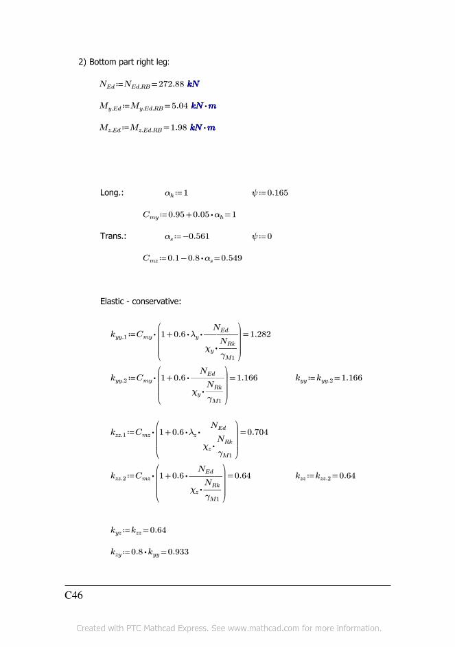
2) Bottom part right leg:
≔NEd =NEd.RB 272.88 kNkNkNkN
≔My.Ed =My.Ed.RB 5.04 ⋅kNkNkNkN mmmm
≔Mz.Ed =Mz.Ed.RB 1.98 ⋅kNkNkNkN mmmm
Long.: ≔αh 1 ≔ψ 0.165
≔Cmy =+0.95 ⋅0.05 αh 1
Trans.: ≔αs −0.561 ≔ψ 0
≔Cmz =−0.1 ⋅0.8 αs 0.549
Elastic - conservative:
≔kyy.1 =⋅Cmy
⎛⎜⎜⎜⎝
+1 ⋅⋅0.6 λy ―――NEd
⋅χy ――NRk
γM1
⎞⎟⎟⎟⎠
1.282
≔kyy.2 =⋅Cmy
⎛⎜⎜⎜⎝
+1 ⋅0.6 ―――NEd
⋅χy ――NRk
γM1
⎞⎟⎟⎟⎠
1.166 ≔kyy =kyy.2 1.166
≔kzz.1 =⋅Cmz
⎛⎜⎜⎜⎝
+1 ⋅⋅0.6 λz ―――NEd
⋅χz ――NRk
γM1
⎞⎟⎟⎟⎠
0.704
≔kzz.2 =⋅Cmz
⎛⎜⎜⎜⎝
+1 ⋅0.6 ―――NEd
⋅χz ――NRk
γM1
⎞⎟⎟⎟⎠
0.64 ≔kzz =kzz.2 0.64
≔kyz =kzz 0.64
≔kzy =⋅0.8 kyy 0.933
C46
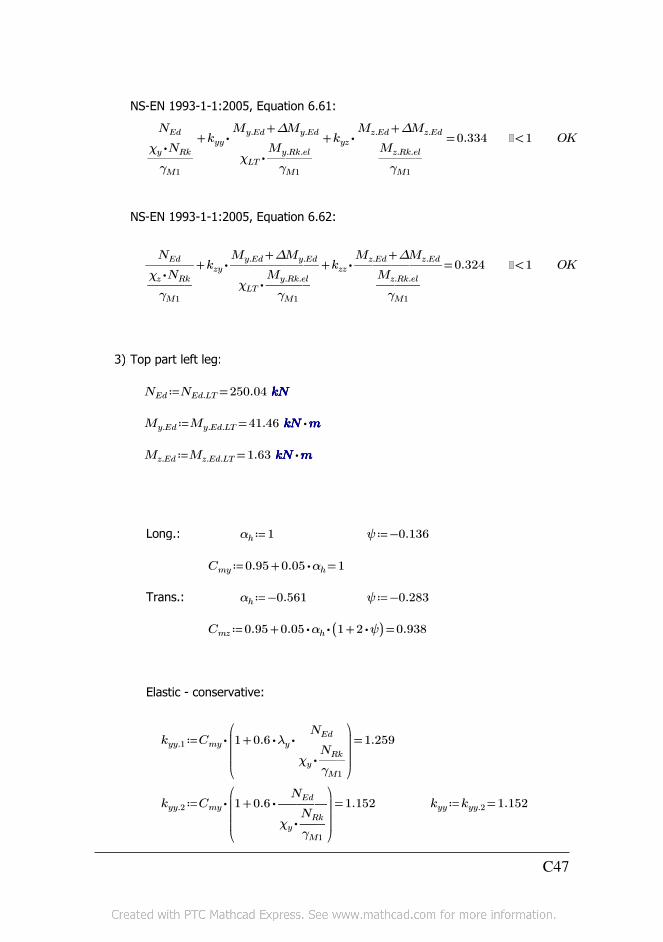
NS-EN 1993-1-1:2005, Equation 6.61:
=++―――NEd
―――⋅χy NRk
γM1
⋅kyy ―――――+My.Ed ∆My.Ed
⋅χLT ―――My.Rk.el
γM1
⋅kyz ―――――+Mz.Ed ∆Mz.Ed
―――Mz.Rk.el
γM1
0.334 <1 OK
NS-EN 1993-1-1:2005, Equation 6.62:
=++―――NEd
―――⋅χz NRk
γM1
⋅kzy ―――――+My.Ed ∆My.Ed
⋅χLT ―――My.Rk.el
γM1
⋅kzz ―――――+Mz.Ed ∆Mz.Ed
―――Mz.Rk.el
γM1
0.324 <1 OK
3) Top part left leg:
≔NEd =NEd.LT 250.04 kNkNkNkN
≔My.Ed =My.Ed.LT 41.46 ⋅kNkNkNkN mmmm
≔Mz.Ed =Mz.Ed.LT 1.63 ⋅kNkNkNkN mmmm
Long.: ≔αh 1 ≔ψ −0.136
≔Cmy =+0.95 ⋅0.05 αh 1
Trans.: ≔αh −0.561 ≔ψ −0.283
≔Cmz =+0.95 ⋅⋅0.05 αh (( +1 ⋅2 ψ)) 0.938
Elastic - conservative:
≔kyy.1 =⋅Cmy
⎛⎜⎜⎜⎝
+1 ⋅⋅0.6 λy ―――NEd
⋅χy ――NRk
γM1
⎞⎟⎟⎟⎠
1.259
≔kyy.2 =⋅Cmy
⎛⎜⎜⎜⎝
+1 ⋅0.6 ―――NEd
⋅χy ――NRk
γM1
⎞⎟⎟⎟⎠
1.152 ≔kyy =kyy.2 1.152
C47

≔kzz.1 =⋅Cmz
⎛⎜⎜⎜⎝
+1 ⋅⋅0.6 λz ―――NEd
⋅χz ――NRk
γM1
⎞⎟⎟⎟⎠
1.18
≔kzz.2 =⋅Cmz
⎛⎜⎜⎜⎝
+1 ⋅0.6 ―――NEd
⋅χz ――NRk
γM1
⎞⎟⎟⎟⎠
1.081 ≔kzz =kzz.2 1.081
≔kyz =kzz 1.081
≔kzy =⋅0.8 kyy 0.922
NS-EN 1993-1-1:2005, Equation 6.61:
=++―――NEd
―――⋅χy NRk
γM1
⋅kyy ―――――+My.Ed ∆My.Ed
⋅χLT ―――My.Rk.el
γM1
⋅kyz ―――――+Mz.Ed ∆Mz.Ed
―――Mz.Rk.el
γM1
0.686 <1 OK
NS-EN 1993-1-1:2005, Equation 6.62:
=++―――NEd
―――⋅χz NRk
γM1
⋅kzy ―――――+My.Ed ∆My.Ed
⋅χLT ―――My.Rk.el
γM1
⋅kzz ―――――+Mz.Ed ∆Mz.Ed
―――Mz.Rk.el
γM1
0.601 <1 OK
4) Bottom part left leg:
≔NEd =NEd.LB 272.52 kNkNkNkN
≔My.Ed =My.Ed.LB 4.99 ⋅kNkNkNkN mmmm
≔Mz.Ed =Mz.Ed.LB 2.08 ⋅kNkNkNkN mmmm
Long.: ≔αh 0.998 ≔ψ 0.169
≔Cmy =+0.95 ⋅0.05 αh 1
0.548 ψ 0Trans.:C48
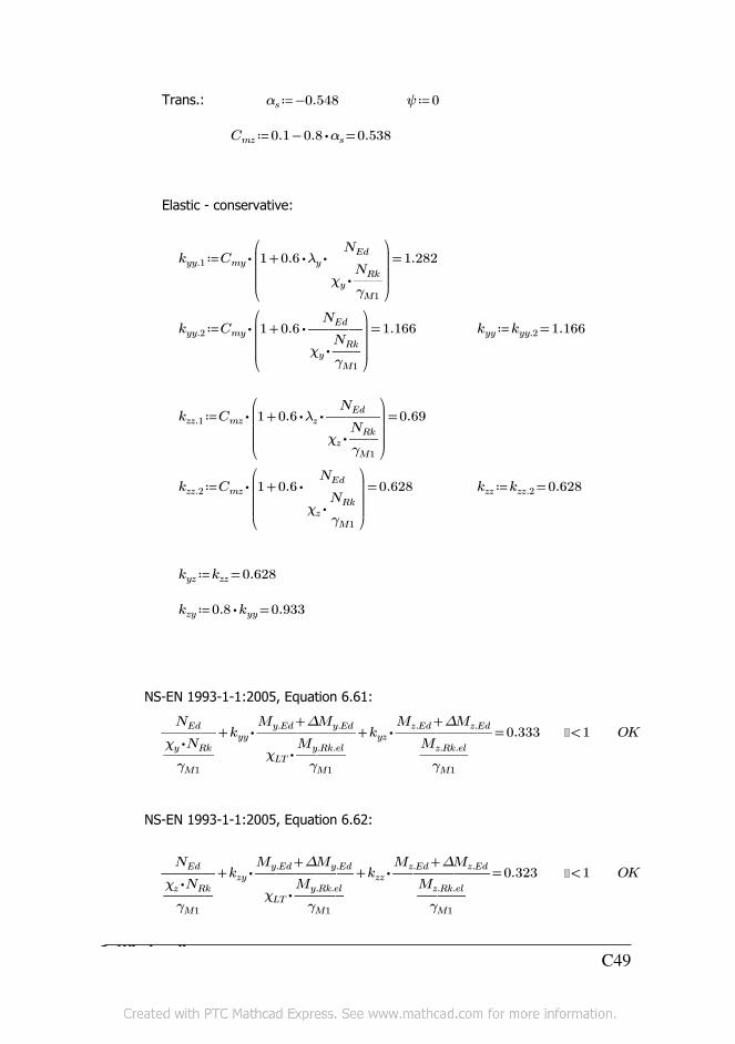
Trans.: ≔αs −0.548 ≔ψ 0
≔Cmz =−0.1 ⋅0.8 αs 0.538
Elastic - conservative:
≔kyy.1 =⋅Cmy
⎛⎜⎜⎜⎝
+1 ⋅⋅0.6 λy ―――NEd
⋅χy ――NRk
γM1
⎞⎟⎟⎟⎠
1.282
≔kyy.2 =⋅Cmy
⎛⎜⎜⎜⎝
+1 ⋅0.6 ―――NEd
⋅χy ――NRk
γM1
⎞⎟⎟⎟⎠
1.166 ≔kyy =kyy.2 1.166
≔kzz.1 =⋅Cmz
⎛⎜⎜⎜⎝
+1 ⋅⋅0.6 λz ―――NEd
⋅χz ――NRk
γM1
⎞⎟⎟⎟⎠
0.69
≔kzz.2 =⋅Cmz
⎛⎜⎜⎜⎝
+1 ⋅0.6 ―――NEd
⋅χz ――NRk
γM1
⎞⎟⎟⎟⎠
0.628 ≔kzz =kzz.2 0.628
≔kyz =kzz 0.628
≔kzy =⋅0.8 kyy 0.933
NS-EN 1993-1-1:2005, Equation 6.61:
=++―――NEd
―――⋅χy NRk
γM1
⋅kyy ―――――+My.Ed ∆My.Ed
⋅χLT ―――My.Rk.el
γM1
⋅kyz ―――――+Mz.Ed ∆Mz.Ed
―――Mz.Rk.el
γM1
0.333 <1 OK
NS-EN 1993-1-1:2005, Equation 6.62:
=++―――NEd
―――⋅χz NRk
γM1
⋅kzy ―――――+My.Ed ∆My.Ed
⋅χLT ―――My.Rk.el
γM1
⋅kzz ―――――+Mz.Ed ∆Mz.Ed
―――Mz.Rk.el
γM1
0.323 <1 OK
2 Wind on line C49
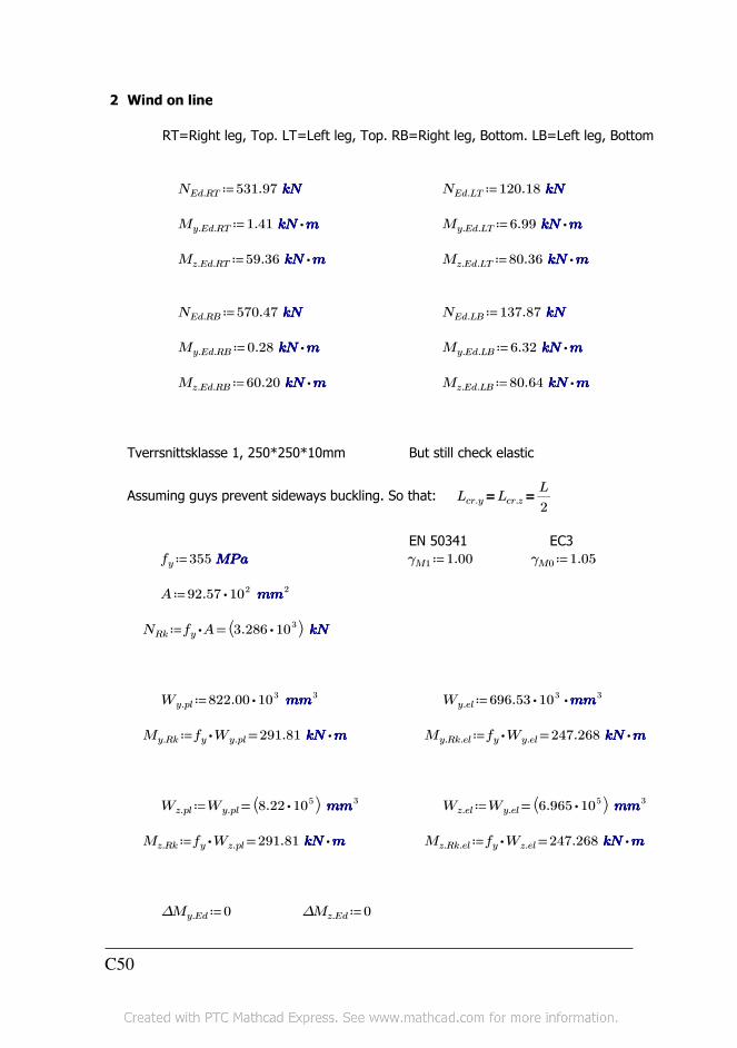
2 Wind on line
RT=Right leg, Top. LT=Left leg, Top. RB=Right leg, Bottom. LB=Left leg, Bottom
≔NEd.RT 531.97 kNkNkNkN ≔NEd.LT 120.18 kNkNkNkN
≔My.Ed.RT ⋅1.41 kNkNkNkN mmmm ≔My.Ed.LT ⋅6.99 kNkNkNkN mmmm
≔Mz.Ed.RT ⋅59.36 kNkNkNkN mmmm ≔Mz.Ed.LT ⋅80.36 kNkNkNkN mmmm
≔NEd.RB 570.47 kNkNkNkN ≔NEd.LB 137.87 kNkNkNkN
≔My.Ed.RB ⋅0.28 kNkNkNkN mmmm ≔My.Ed.LB ⋅6.32 kNkNkNkN mmmm
≔Mz.Ed.RB ⋅60.20 kNkNkNkN mmmm ≔Mz.Ed.LB ⋅80.64 kNkNkNkN mmmm
Tverrsnittsklasse 1, 250*250*10mm But still check elastic
Assuming guys prevent sideways buckling. So that: ==Lcr.y Lcr.z ―L
2
EN 50341 EC3
≔fy 355 MPaMPaMPaMPa ≔γM1 1.00 ≔γM0 1.05
≔A ⋅92.57 102 mmmmmmmm2
≔NRk =⋅fy A ⎛⎝ ⋅3.286 103 ⎞⎠ kNkNkNkN
≔Wy.pl ⋅822.00 103 mmmmmmmm3 ≔Wy.el ⋅⋅696.53 103 mmmmmmmm3
≔My.Rk =⋅fy Wy.pl 291.81 ⋅kNkNkNkN mmmm ≔My.Rk.el =⋅fy Wy.el 247.268 ⋅kNkNkNkN mmmm
≔Wz.pl =Wy.pl⎛⎝ ⋅8.22 105 ⎞⎠ mmmmmmmm3 ≔Wz.el =Wy.el
⎛⎝ ⋅6.965 105 ⎞⎠ mmmmmmmm3
≔Mz.Rk =⋅fy Wz.pl 291.81 ⋅kNkNkNkN mmmm ≔Mz.Rk.el =⋅fy Wz.el 247.268 ⋅kNkNkNkN mmmm
≔∆My.Ed 0 ≔∆Mz.Ed 0
C50

Clause 6.3.1.3:
≔E 210000 MPaMPaMPaMPa ≔I ⋅8706.67 104 mmmmmmmm4
≔L 25.19 mmmm ≔Lcr =―L
212.595 mmmm
≔Ncr.y =―――⋅⋅ππππ
2 E I
Lcr2
⎛⎝ ⋅1.138 103 ⎞⎠ kNkNkNkN ≔Ncr.z =―――⋅⋅ππππ
2 E I
Lcr2
⎛⎝ ⋅1.138 103 ⎞⎠ kNkNkNkN
≔λy =‾‾‾‾‾――NRk
Ncr.y
1.7 ≔λz =‾‾‾‾‾――NRk
Ncr.z
1.7
≔χy 0.3Warm formed: Buckling curve a in figure 6.4
≔χz 0.3
Clause 6.3.2.3:
≔Mc.Rd =⋅Wy.el ――fy
γM0
235.493 ⋅kNkNkNkN mmmm
Other cross section: Buckling curve d ≔αLT 0.76
≔λLT =‾‾‾‾‾‾‾―――
⋅Wy.el fy
Mc.Rd
1.025
≔ΦLT =⋅0.5 ⎛⎝ ++1 ⋅αLT ⎛⎝ −λLT 0.2⎞⎠ λLT2 ⎞⎠ 1.338
≔χLT =―――――――1
+ΦLT‾‾‾‾‾‾‾‾‾‾−ΦLT
2 λLT2
0.455
Annex B:
1) Top part right leg:
≔NEd =NEd.RT 531.97 kNkNkNkN
≔My.Ed =My.Ed.RT 1.41 ⋅kNkNkNkN mmmm
≔Mz.Ed =Mz.Ed.RT 59.36 ⋅kNkNkNkN mmmm
0.972 ψ 0.015Long.: C51

Long.: ≔αh 0.972 ≔ψ −0.015
≔Cmy =+0.95 ⋅0.05 αh 0.999
Trans.: ≔αh 0.986 ≔ψ 0
≔Cmz =+0.95 ⋅0.05 αh 0.999
Elastic - conservative:
≔kyy.1 =⋅Cmy
⎛⎜⎜⎜⎝
+1 ⋅⋅0.6 λy ―――NEd
⋅χy ――NRk
γM1
⎞⎟⎟⎟⎠
1.548
≔kyy.2 =⋅Cmy
⎛⎜⎜⎜⎝
+1 ⋅0.6 ―――NEd
⋅χy ――NRk
γM1
⎞⎟⎟⎟⎠
1.322 ≔kyy =kyy.2 1.322
≔kzz.1 =⋅Cmz
⎛⎜⎜⎜⎝
+1 ⋅⋅0.6 λz ―――NEd
⋅χz ――NRk
γM1
⎞⎟⎟⎟⎠
1.549
≔kzz.2 =⋅Cmz
⎛⎜⎜⎜⎝
+1 ⋅0.6 ―――NEd
⋅χz ――NRk
γM1
⎞⎟⎟⎟⎠
1.323 ≔kzz =kzz.2 1.323
≔kyz =kzz 1.323 ≔kzy =⋅0.8 kyy 1.058
NS-EN 1993-1-1:2005, Equation 6.61:
=++―――NEd
―――⋅χy NRk
γM1
⋅kyy ―――――+My.Ed ∆My.Ed
⋅χLT ―――My.Rk.el
γM1
⋅kyz ―――――+Mz.Ed ∆Mz.Ed
―――Mz.Rk.el
γM1
0.874 <1 OK
NS-EN 1993-1-1:2005, Equation 6.62:
=++―――NEd
―――⋅χz NRk
γM1
⋅kzy ―――――+My.Ed ∆My.Ed
⋅χLT ―――My.Rk.el
γM1
⋅kzz ―――――+Mz.Ed ∆Mz.Ed
―――Mz.Rk.el
γM1
0.87 <1 OK
2) Bottom part right leg:C52
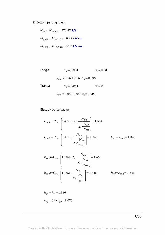
2) Bottom part right leg:
≔NEd =NEd.RB 570.47 kNkNkNkN
≔My.Ed =My.Ed.RB 0.28 ⋅kNkNkNkN mmmm
≔Mz.Ed =Mz.Ed.RB 60.2 ⋅kNkNkNkN mmmm
Long.: ≔αh 0.964 ≔ψ 0.33
≔Cmy =+0.95 ⋅0.05 αh 0.998
Trans.: ≔αh 0.984 ≔ψ 0
≔Cmz =+0.95 ⋅0.05 αh 0.999
Elastic - conservative:
≔kyy.1 =⋅Cmy
⎛⎜⎜⎜⎝
+1 ⋅⋅0.6 λy ―――NEd
⋅χy ――NRk
γM1
⎞⎟⎟⎟⎠
1.587
≔kyy.2 =⋅Cmy
⎛⎜⎜⎜⎝
+1 ⋅0.6 ―――NEd
⋅χy ――NRk
γM1
⎞⎟⎟⎟⎠
1.345 ≔kyy =kyy.2 1.345
≔kzz.1 =⋅Cmz
⎛⎜⎜⎜⎝
+1 ⋅⋅0.6 λz ―――NEd
⋅χz ――NRk
γM1
⎞⎟⎟⎟⎠
1.589
≔kzz.2 =⋅Cmz
⎛⎜⎜⎜⎝
+1 ⋅0.6 ―――NEd
⋅χz ――NRk
γM1
⎞⎟⎟⎟⎠
1.346 ≔kzz =kzz.2 1.346
≔kyz =kzz 1.346
≔kzy =⋅0.8 kyy 1.076
C53
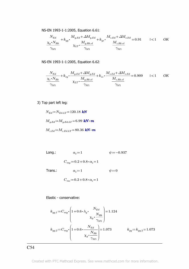
NS-EN 1993-1-1:2005, Equation 6.61:
=++―――NEd
―――⋅χy NRk
γM1
⋅kyy ―――――+My.Ed ∆My.Ed
⋅χLT ―――My.Rk.el
γM1
⋅kyz ―――――+Mz.Ed ∆Mz.Ed
―――Mz.Rk.el
γM1
0.91 <1 OK
NS-EN 1993-1-1:2005, Equation 6.62:
=++―――NEd
―――⋅χz NRk
γM1
⋅kzy ―――――+My.Ed ∆My.Ed
⋅χLT ―――My.Rk.el
γM1
⋅kzz ―――――+Mz.Ed ∆Mz.Ed
―――Mz.Rk.el
γM1
0.909 <1 OK
3) Top part left leg:
≔NEd =NEd.LT 120.18 kNkNkNkN
≔My.Ed =My.Ed.LT 6.99 ⋅kNkNkNkN mmmm
≔Mz.Ed =Mz.Ed.LT 80.36 ⋅kNkNkNkN mmmm
Long.: ≔αs 1 ≔ψ −0.937
≔Cmy =+0.2 ⋅0.8 αs 1
Trans.: ≔αs 1 ≔ψ 0
≔Cmz =+0.2 ⋅0.8 αs 1
Elastic - conservative:
≔kyy.1 =⋅Cmy
⎛⎜⎜⎜⎝
+1 ⋅⋅0.6 λy ―――NEd
⋅χy ――NRk
γM1
⎞⎟⎟⎟⎠
1.124
≔kyy.2 =⋅Cmy
⎛⎜⎜⎜⎝
+1 ⋅0.6 ―――NEd
⋅χy ――NRk
γM1
⎞⎟⎟⎟⎠
1.073 ≔kyy =kyy.2 1.073
C54
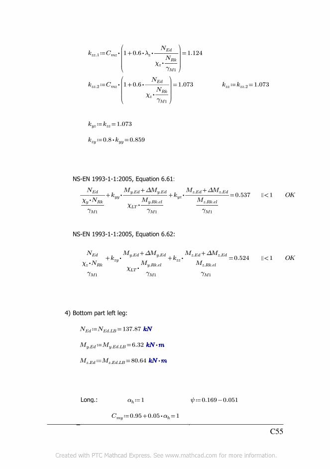
≔kzz.1 =⋅Cmz
⎛⎜⎜⎜⎝
+1 ⋅⋅0.6 λz ―――NEd
⋅χz ――NRk
γM1
⎞⎟⎟⎟⎠
1.124
≔kzz.2 =⋅Cmz
⎛⎜⎜⎜⎝
+1 ⋅0.6 ―――NEd
⋅χz ――NRk
γM1
⎞⎟⎟⎟⎠
1.073 ≔kzz =kzz.2 1.073
≔kyz =kzz 1.073
≔kzy =⋅0.8 kyy 0.859
NS-EN 1993-1-1:2005, Equation 6.61:
=++―――NEd
―――⋅χy NRk
γM1
⋅kyy ―――――+My.Ed ∆My.Ed
⋅χLT ―――My.Rk.el
γM1
⋅kyz ―――――+Mz.Ed ∆Mz.Ed
―――Mz.Rk.el
γM1
0.537 <1 OK
NS-EN 1993-1-1:2005, Equation 6.62:
=++―――NEd
―――⋅χz NRk
γM1
⋅kzy ―――――+My.Ed ∆My.Ed
⋅χLT ―――My.Rk.el
γM1
⋅kzz ―――――+Mz.Ed ∆Mz.Ed
―――Mz.Rk.el
γM1
0.524 <1 OK
4) Bottom part left leg:
≔NEd =NEd.LB 137.87 kNkNkNkN
≔My.Ed =My.Ed.LB 6.32 ⋅kNkNkNkN mmmm
≔Mz.Ed =Mz.Ed.LB 80.64 ⋅kNkNkNkN mmmm
Long.: ≔αh 1 ≔ψ −0.169 0.051
≔Cmy =+0.95 ⋅0.05 αh 1
1 ψ 0Trans.: C55

Trans.: ≔αs 1 ≔ψ 0
≔Cmz =+0.2 ⋅0.8 αs 1
Elastic - conservative:
≔kyy.1 =⋅Cmy
⎛⎜⎜⎜⎝
+1 ⋅⋅0.6 λy ―――NEd
⋅χy ――NRk
γM1
⎞⎟⎟⎟⎠
1.143
≔kyy.2 =⋅Cmy
⎛⎜⎜⎜⎝
+1 ⋅0.6 ―――NEd
⋅χy ――NRk
γM1
⎞⎟⎟⎟⎠
1.084 ≔kyy =kyy.2 1.084
≔kzz.1 =⋅Cmz
⎛⎜⎜⎜⎝
+1 ⋅⋅0.6 λz ―――NEd
⋅χz ――NRk
γM1
⎞⎟⎟⎟⎠
1.143
≔kzz.2 =⋅Cmz
⎛⎜⎜⎜⎝
+1 ⋅0.6 ―――NEd
⋅χz ――NRk
γM1
⎞⎟⎟⎟⎠
1.084 ≔kzz =kzz.2 1.084
≔kyz =kzz 1.084
≔kzy =⋅0.8 kyy 0.867
NS-EN 1993-1-1:2005, Equation 6.61:
=++―――NEd
―――⋅χy NRk
γM1
⋅kyy ―――――+My.Ed ∆My.Ed
⋅χLT ―――My.Rk.el
γM1
⋅kyz ―――――+Mz.Ed ∆Mz.Ed
―――Mz.Rk.el
γM1
0.554 <1 OK
NS-EN 1993-1-1:2005, Equation 6.62:
=++―――NEd
―――⋅χz NRk
γM1
⋅kzy ―――――+My.Ed ∆My.Ed
⋅χLT ―――My.Rk.el
γM1
⋅kzz ―――――+Mz.Ed ∆Mz.Ed
―――Mz.Rk.el
γM1
0.542 <1 OK
C56
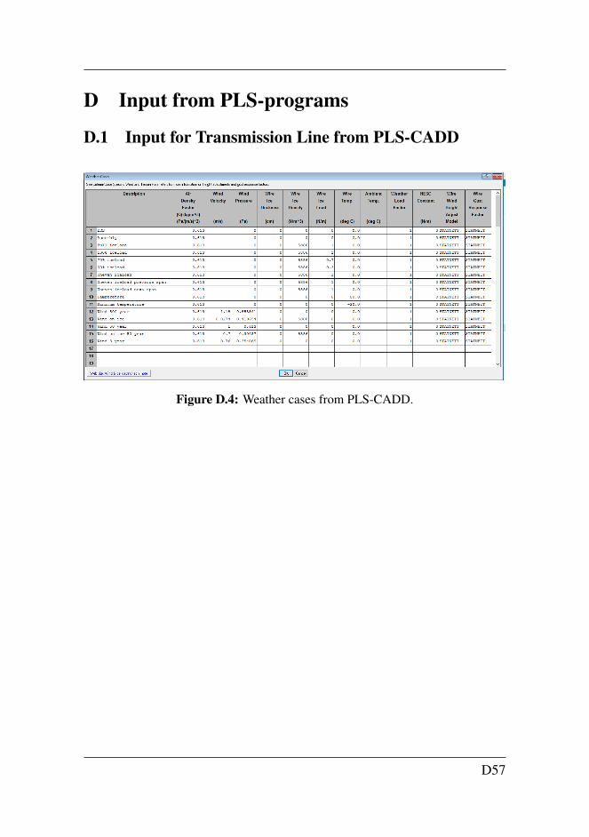
D Input from PLS-programs
D.1 Input for Transmission Line from PLS-CADD
Figure D.4: Weather cases from PLS-CADD.
D57
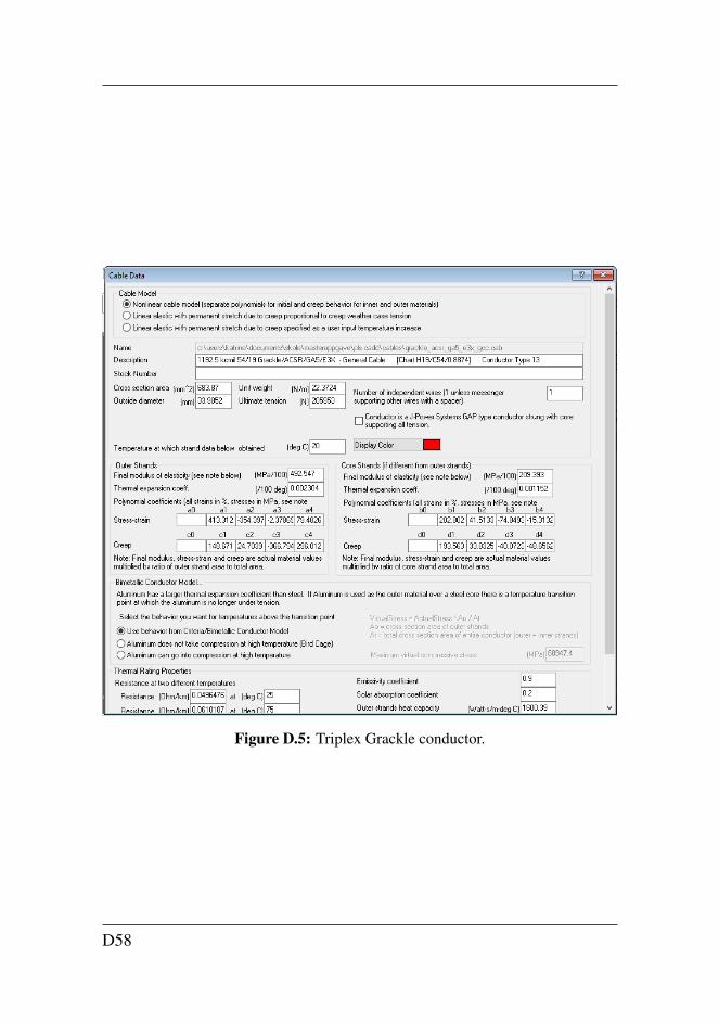
Figure D.5: Triplex Grackle conductor.
D58
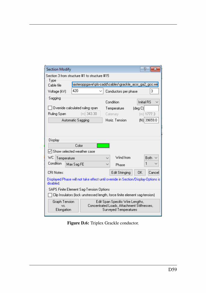
Figure D.6: Triplex Grackle conductor.
D59
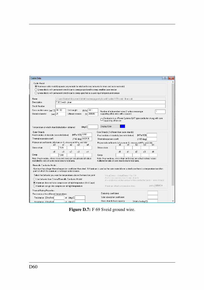
Figure D.7: F 69 Sveid ground wire.
D60
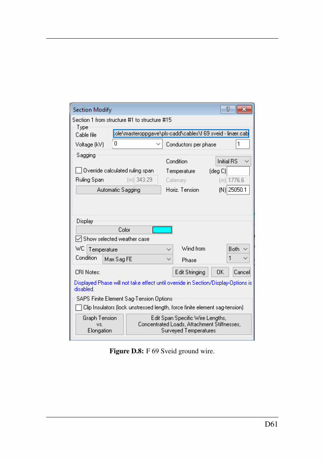
Figure D.8: F 69 Sveid ground wire.
D61
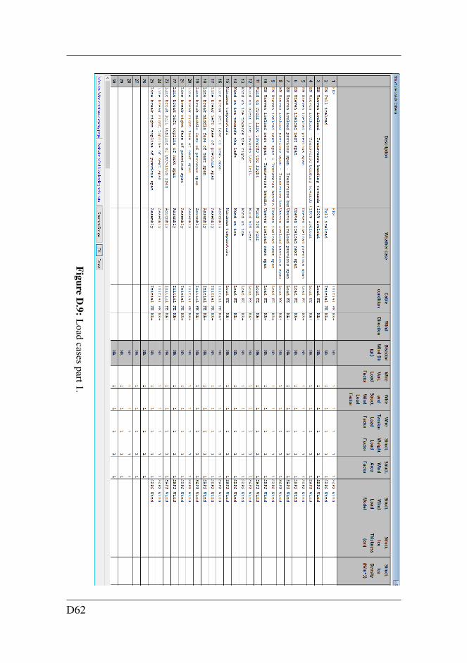
FigureD
.9:L
oadcases
part1.
D62
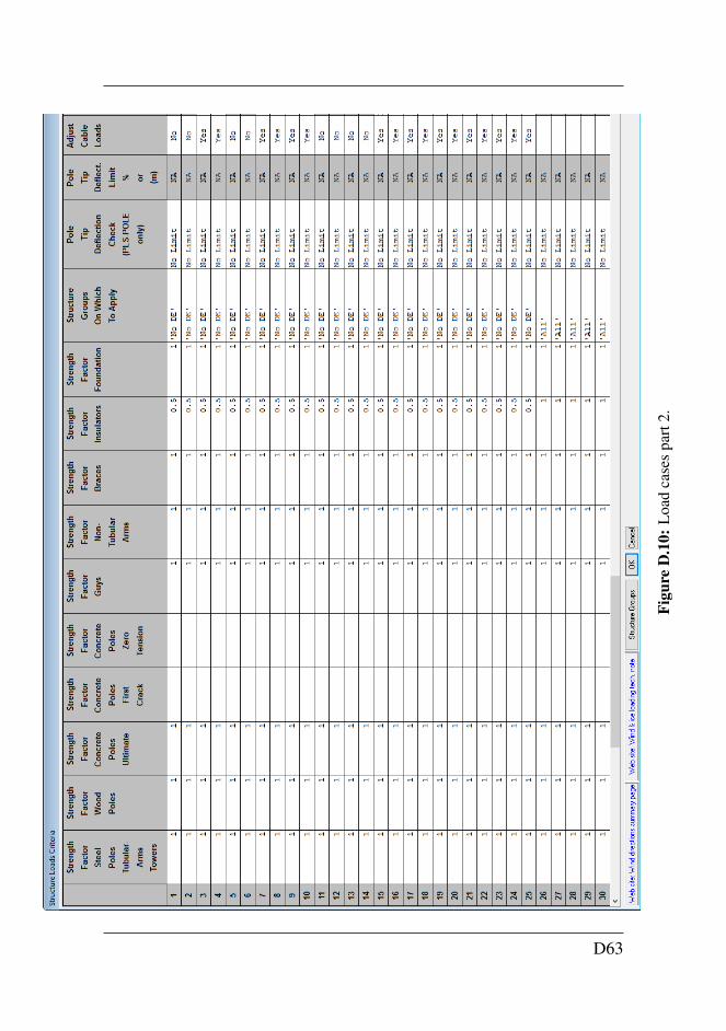
Figu
reD
.10:
Loa
dca
ses
part
2.
D63
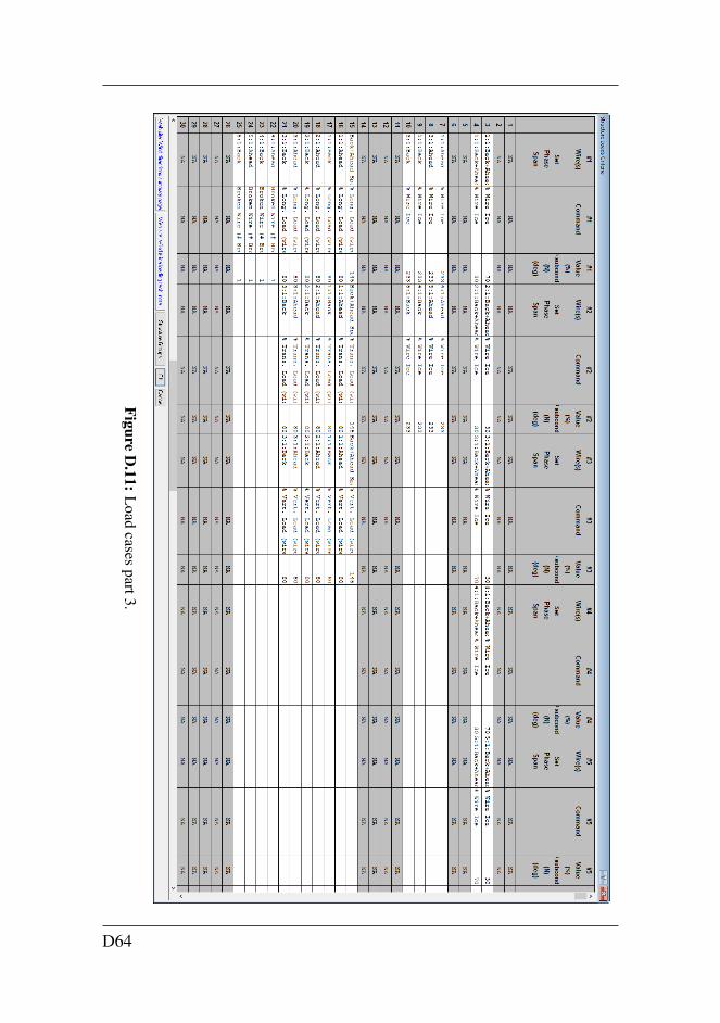
FigureD
.11:L
oadcases
part3.
D64
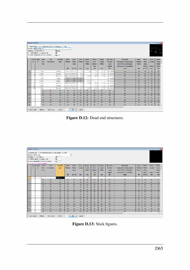
Figure D.12: Dead end structures.
Figure D.13: Stick figures.
D65
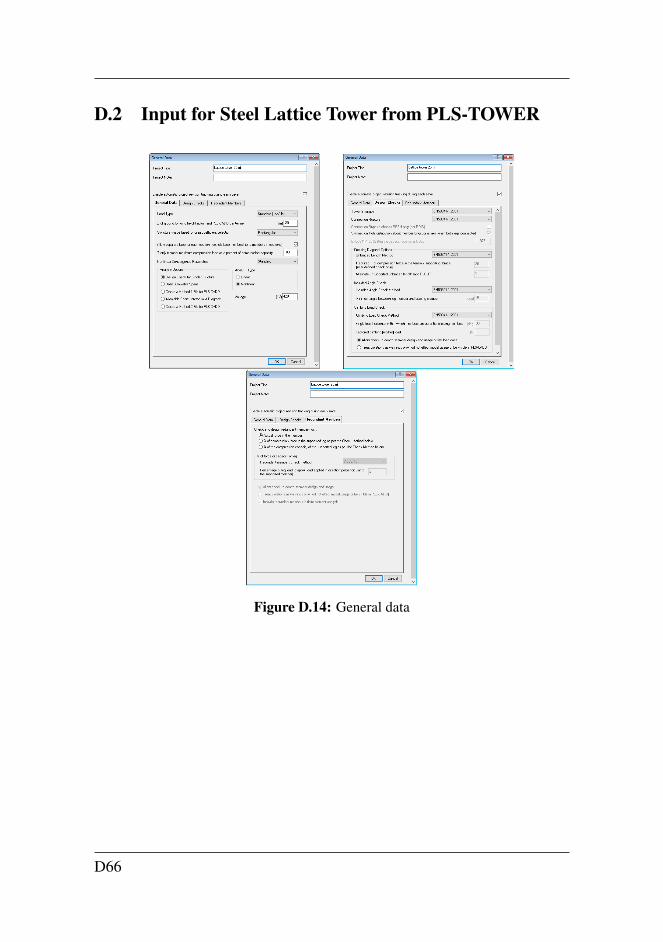
D.2 Input for Steel Lattice Tower from PLS-TOWER
Figure D.14: General data
D66
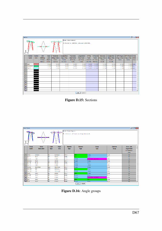
Figure D.15: Sections
Figure D.16: Angle groups
D67
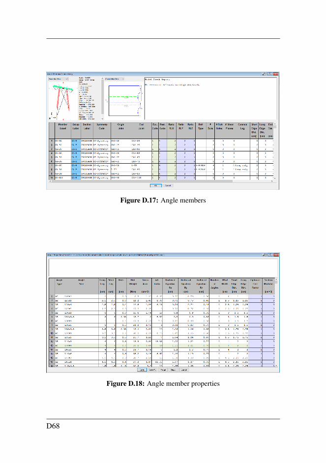
Figure D.17: Angle members
Figure D.18: Angle member properties
D68
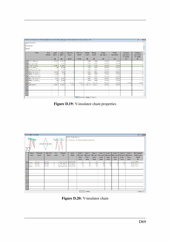
Figure D.19: V-insulator chain properties
Figure D.20: V-insulator chain
D69
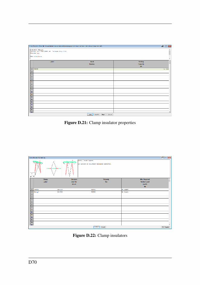
Figure D.21: Clamp insulator properties
Figure D.22: Clamp insulators
D70
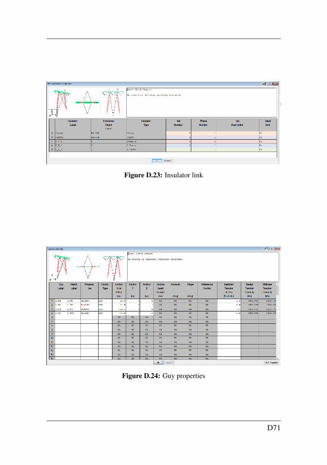
Figure D.23: Insulator link
Figure D.24: Guy properties
D71
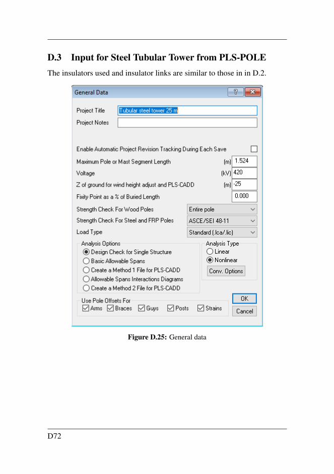
D.3 Input for Steel Tubular Tower from PLS-POLEThe insulators used and insulator links are similar to those in in D.2.
Figure D.25: General data
D72
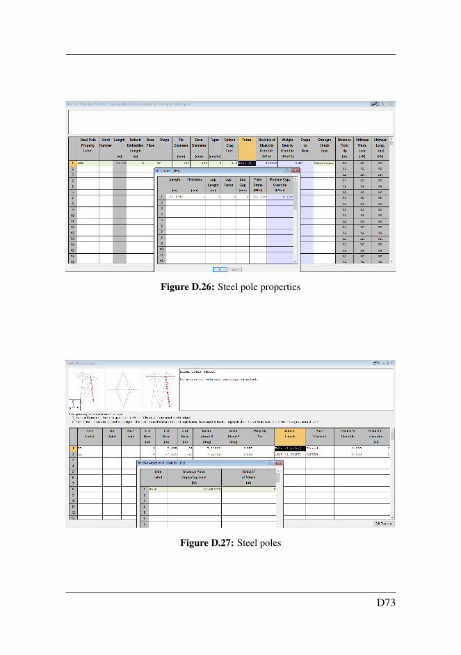
Figure D.26: Steel pole properties
Figure D.27: Steel poles
D73
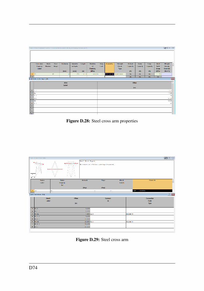
Figure D.28: Steel cross arm properties
Figure D.29: Steel cross arm
D74
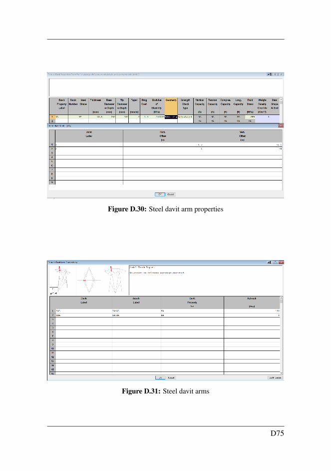
Figure D.30: Steel davit arm properties
Figure D.31: Steel davit arms
D75
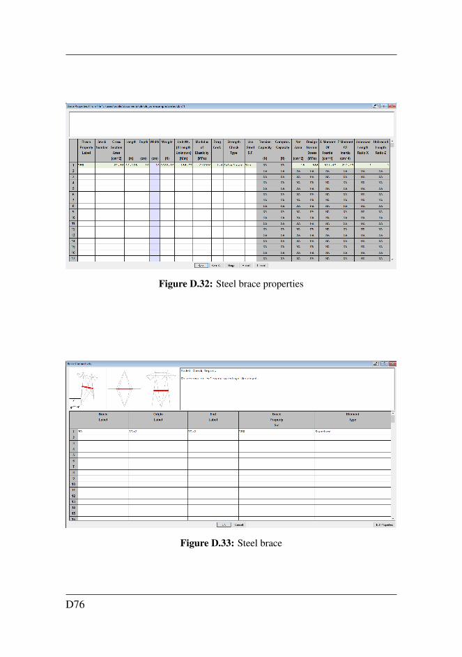
Figure D.32: Steel brace properties
Figure D.33: Steel brace
D76
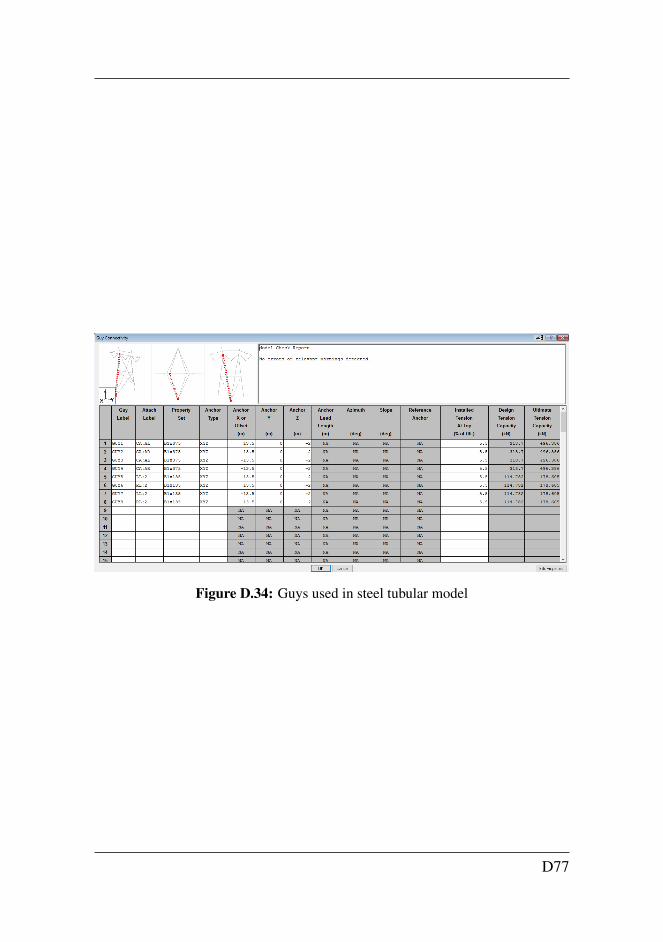
Figure D.34: Guys used in steel tubular model
D77

D.4 Input for FRP Tubular Tower from PLS-POLEThe insulators used and insulator links are similar to those in in D.2.
Figure D.35: General data
D78
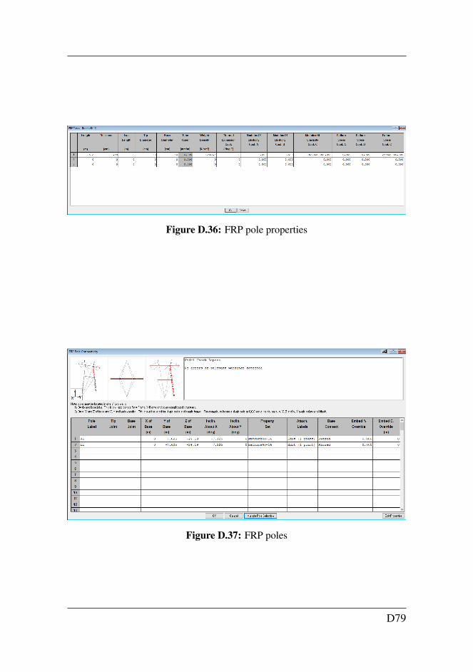
Figure D.36: FRP pole properties
Figure D.37: FRP poles
D79
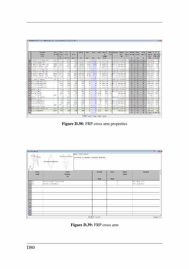
Figure D.38: FRP cross arm properties
Figure D.39: FRP cross arm
D80
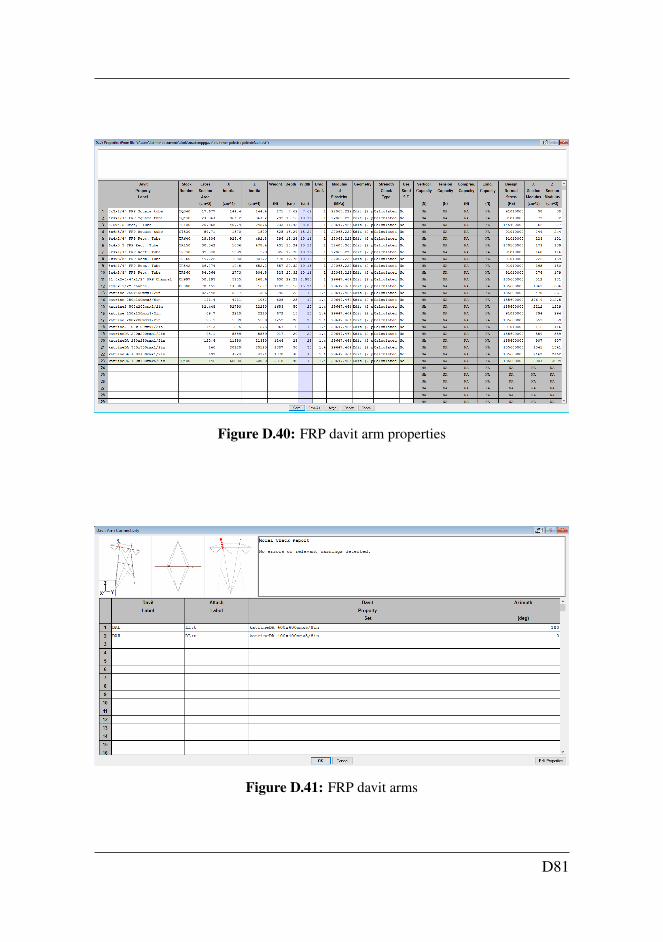
Figure D.40: FRP davit arm properties
Figure D.41: FRP davit arms
D81
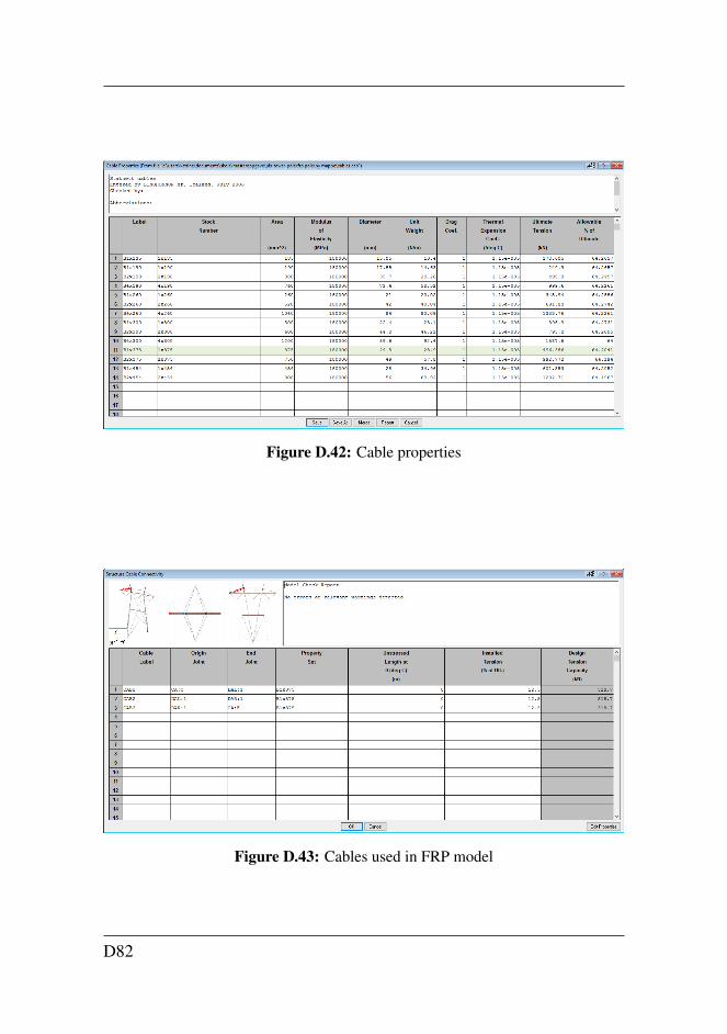
Figure D.42: Cable properties
Figure D.43: Cables used in FRP model
D82
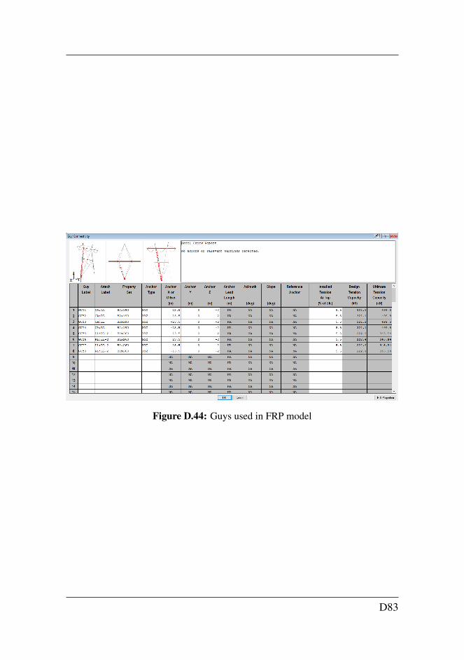
Figure D.44: Guys used in FRP model
D83

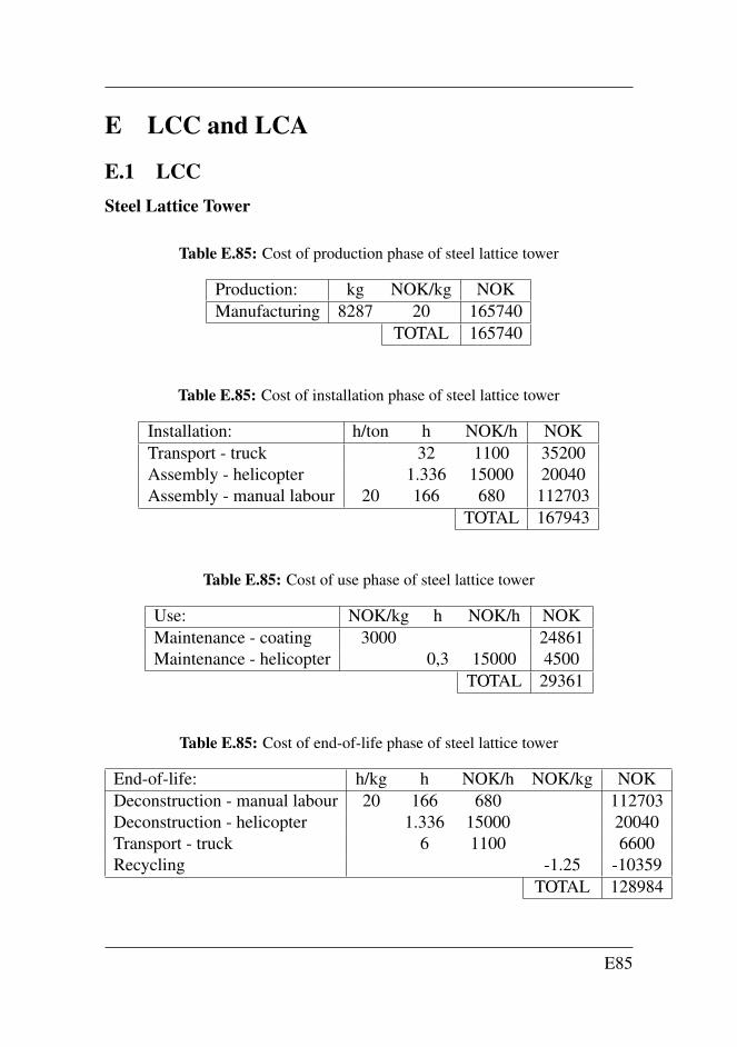
E LCC and LCA
E.1 LCCSteel Lattice Tower
Table E.85: Cost of production phase of steel lattice tower
Production: kg NOK/kg NOKManufacturing 8287 20 165740
TOTAL 165740
Table E.85: Cost of installation phase of steel lattice tower
Installation: h/ton h NOK/h NOKTransport - truck 32 1100 35200Assembly - helicopter 1.336 15000 20040Assembly - manual labour 20 166 680 112703
TOTAL 167943
Table E.85: Cost of use phase of steel lattice tower
Use: NOK/kg h NOK/h NOKMaintenance - coating 3000 24861Maintenance - helicopter 0,3 15000 4500
TOTAL 29361
Table E.85: Cost of end-of-life phase of steel lattice tower
End-of-life: h/kg h NOK/h NOK/kg NOKDeconstruction - manual labour 20 166 680 112703Deconstruction - helicopter 1.336 15000 20040Transport - truck 6 1100 6600Recycling -1.25 -10359
TOTAL 128984
E85
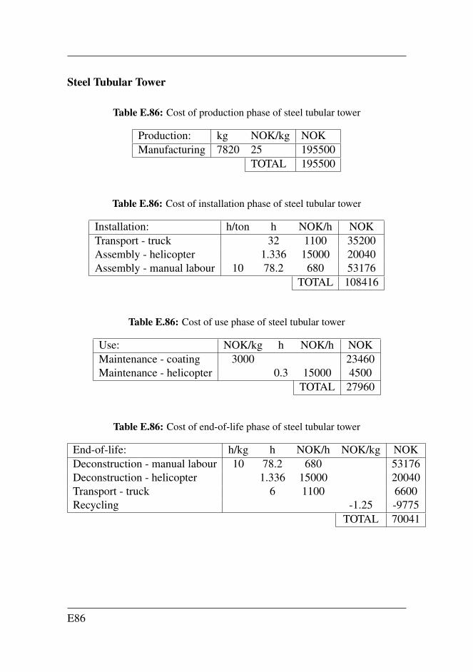
Steel Tubular Tower
Table E.86: Cost of production phase of steel tubular tower
Production: kg NOK/kg NOKManufacturing 7820 25 195500
TOTAL 195500
Table E.86: Cost of installation phase of steel tubular tower
Installation: h/ton h NOK/h NOKTransport - truck 32 1100 35200Assembly - helicopter 1.336 15000 20040Assembly - manual labour 10 78.2 680 53176
TOTAL 108416
Table E.86: Cost of use phase of steel tubular tower
Use: NOK/kg h NOK/h NOKMaintenance - coating 3000 23460Maintenance - helicopter 0.3 15000 4500
TOTAL 27960
Table E.86: Cost of end-of-life phase of steel tubular tower
End-of-life: h/kg h NOK/h NOK/kg NOKDeconstruction - manual labour 10 78.2 680 53176Deconstruction - helicopter 1.336 15000 20040Transport - truck 6 1100 6600Recycling -1.25 -9775
TOTAL 70041
E86
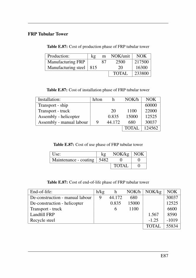
FRP Tubular Tower
Table E.87: Cost of production phase of FRP tubular tower
Production: kg m NOK/unit NOKManufacturing FRP 87 2500 217500Manufacturing steel 815 20 16300
TOTAL 233800
Table E.87: Cost of installation phase of FRP tubular tower
Installation: h/ton h NOK/h NOKTransport - ship 60000Transport - truck 20 1100 22000Assembly - helicopter 0.835 15000 12525Assembly - manual labour 9 44.172 680 30037
TOTAL 124562
Table E.87: Cost of use phase of FRP tubular tower
Use: kg NOK/kg NOKMaintenance - coating 5482 0 0
TOTAL 0
Table E.87: Cost of end-of-life phase of FRP tubular tower
End-of-life: h/kg h NOK/h NOK/kg NOKDe-construction - manual labour 9 44.172 680 30037De-construction - helicopter 0.835 15000 12525Transport - truck 6 1100 6600Landfill FRP 1.567 8590Recycle steel -1.25 -1019
TOTAL 55834
E87
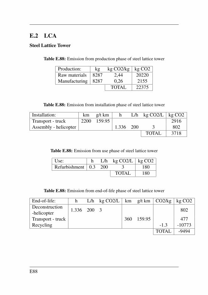
E.2 LCASteel Lattice Tower
Table E.88: Emission from production phase of steel lattice tower
Production: kg kg CO2/kg kg CO2Raw materials 8287 2,44 20220Manufacturing 8287 0,26 2155
TOTAL 22375
Table E.88: Emission from installation phase of steel lattice tower
Installation: km g/t km h L/h kg CO2/L kg CO2Transport - truck 2200 159.95 2916Assembly - helicopter 1.336 200 3 802
TOTAL 3718
Table E.88: Emission from use phase of steel lattice tower
Use: h L/h kg CO2/L kg CO2Refurbishment 0.3 200 3 180
TOTAL 180
Table E.88: Emission from end-of-life phase of steel lattice tower
End-of-life: h L/h kg CO2/L km g/t km CO2/kg kg CO2Deconstruction-helicopter 1.336 200 3 802
Transport - truck 360 159.95 477Recycling -1.3 -10773
TOTAL -9494
E88
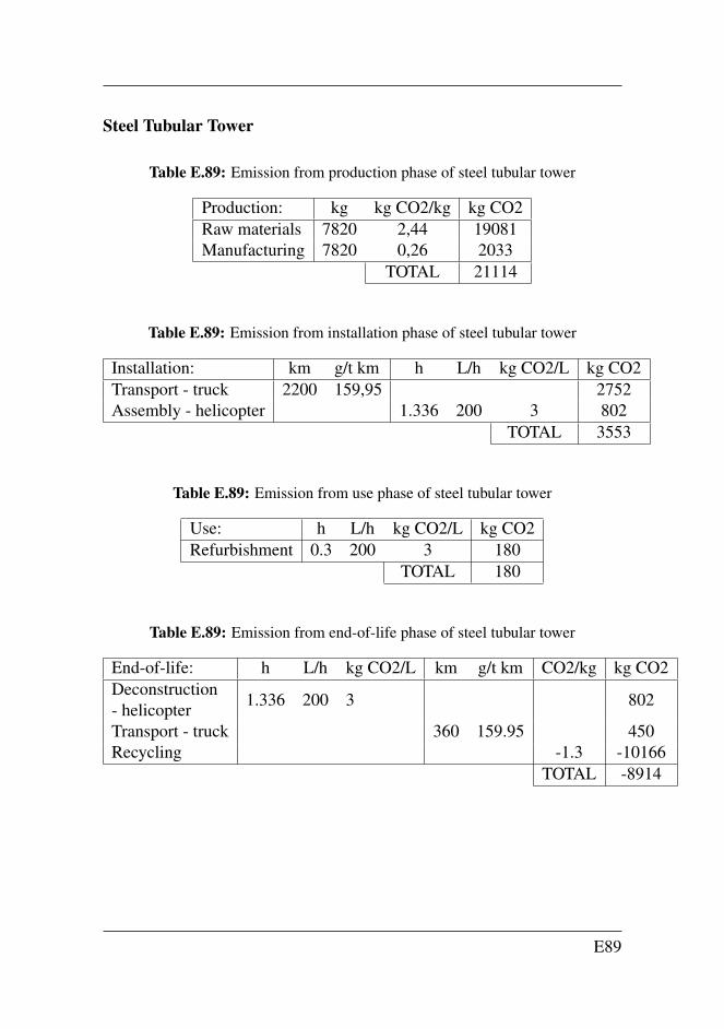
Steel Tubular Tower
Table E.89: Emission from production phase of steel tubular tower
Production: kg kg CO2/kg kg CO2Raw materials 7820 2,44 19081Manufacturing 7820 0,26 2033
TOTAL 21114
Table E.89: Emission from installation phase of steel tubular tower
Installation: km g/t km h L/h kg CO2/L kg CO2Transport - truck 2200 159,95 2752Assembly - helicopter 1.336 200 3 802
TOTAL 3553
Table E.89: Emission from use phase of steel tubular tower
Use: h L/h kg CO2/L kg CO2Refurbishment 0.3 200 3 180
TOTAL 180
Table E.89: Emission from end-of-life phase of steel tubular tower
End-of-life: h L/h kg CO2/L km g/t km CO2/kg kg CO2Deconstruction- helicopter 1.336 200 3 802
Transport - truck 360 159.95 450Recycling -1.3 -10166
TOTAL -8914
E89
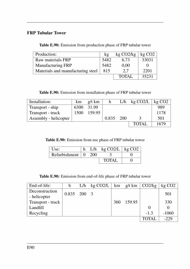
FRP Tubular Tower
Table E.90: Emission from production phase of FRP tubular tower
Production: kg kg CO2/kg kg CO2Raw materials FRP 5482 6,73 33031Manufacturing FRP 5482 0,00 0Materials and manufacturing steel 815 2,7 2201
TOTAL 35231
Table E.90: Emission from installation phase of FRP tubular tower
Installation: km g/t km h L/h kg CO2/L kg CO2Transport - ship 6300 31.99 989Transport - truck 1500 159.95 1178Assembly - helicopter 0.835 200 3 501
TOTAL 1679
Table E.90: Emission from use phase of FRP tubular tower
Use: h L/h kg CO2/L kg CO2Refurbishment 0 200 3 0
TOTAL 0
Table E.90: Emission from end-of-life phase of FRP tubular tower
End-of-life: h L/h kg CO2/L km g/t km CO2/kg kg CO2Deconstruction- helicopter 0.835 200 3 501
Transport - truck 360 159.95 330Landfill 0 0Recycling -1.3 -1060
TOTAL -229
E90
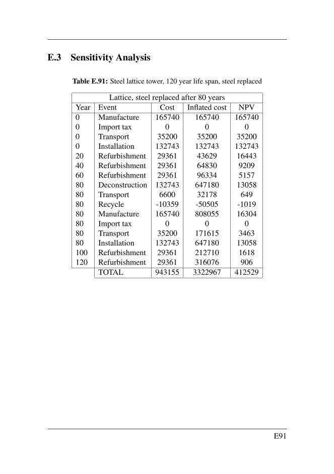
E.3 Sensitivity Analysis
Table E.91: Steel lattice tower, 120 year life span, steel replaced
Lattice, steel replaced after 80 yearsYear Event Cost Inflated cost NPV0 Manufacture 165740 165740 1657400 Import tax 0 0 00 Transport 35200 35200 352000 Installation 132743 132743 13274320 Refurbishment 29361 43629 1644340 Refurbishment 29361 64830 920960 Refurbishment 29361 96334 515780 Deconstruction 132743 647180 1305880 Transport 6600 32178 64980 Recycle -10359 -50505 -101980 Manufacture 165740 808055 1630480 Import tax 0 0 080 Transport 35200 171615 346380 Installation 132743 647180 13058100 Refurbishment 29361 212710 1618120 Refurbishment 29361 316076 906
TOTAL 943155 3322967 412529
E91
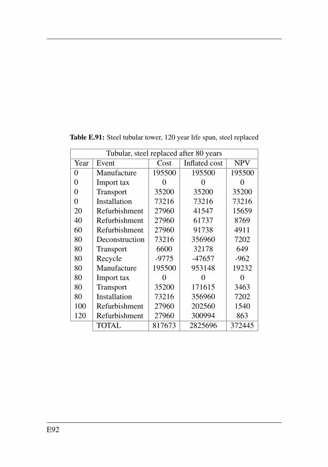
Table E.91: Steel tubular tower, 120 year life span, steel replaced
Tubular, steel replaced after 80 yearsYear Event Cost Inflated cost NPV0 Manufacture 195500 195500 1955000 Import tax 0 0 00 Transport 35200 35200 352000 Installation 73216 73216 7321620 Refurbishment 27960 41547 1565940 Refurbishment 27960 61737 876960 Refurbishment 27960 91738 491180 Deconstruction 73216 356960 720280 Transport 6600 32178 64980 Recycle -9775 -47657 -96280 Manufacture 195500 953148 1923280 Import tax 0 0 080 Transport 35200 171615 346380 Installation 73216 356960 7202100 Refurbishment 27960 202560 1540120 Refurbishment 27960 300994 863
TOTAL 817673 2825696 372445
E92
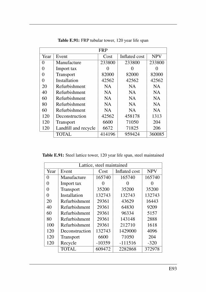
Table E.91: FRP tubular tower, 120 year life span
FRPYear Event Cost Inflated cost NPV0 Manufacture 233800 233800 2338000 Import tax 0 0 00 Transport 82000 82000 820000 Installation 42562 42562 4256220 Refurbishment NA NA NA40 Refurbishment NA NA NA60 Refurbishment NA NA NA80 Refurbishment NA NA NA60 Refurbishment NA NA NA120 Deconstruction 42562 458178 1313120 Transport 6600 71050 204120 Landfill and recycle 6672 71825 206
TOTAL 414196 959424 360085
Table E.91: Steel lattice tower, 120 year life span, steel maintained
Lattice, steel maintainedYear Event Cost Inflated cost NPV0 Manufacture 165740 165740 1657400 Import tax 0 0 00 Transport 35200 35200 352000 Installation 132743 132743 13274320 Refurbishment 29361 43629 1644340 Refurbishment 29361 64830 920960 Refurbishment 29361 96334 515780 Refurbishment 29361 143148 2888100 Refurbishment 29361 212710 1618120 Deconstruction 132743 1429000 4096120 Transport 6600 71050 204120 Recycle -10359 -111516 -320
TOTAL 609472 2282868 372978
E93

Table E.91: Steel lattice tower, 120 year life span, steel maintained
Tubular, steel maintainedYear Event Cost Inflated cost NPV
0 Manufacture 195500 195500 1955000 Import tax 0 0 00 Transport 35200 35200 352000 Installation 73216 73216 73216
20 Refurbishment 27960 41547 1565940 Refurbishment 27960 61737 876960 Refurbishment 27960 91738 491180 Refurbishment 27960 136317 2750100 Refurbishment 27960 202560 1540120 Deconstruction 73216 788182 2259120 Transport 6600 71050 204120 Recycle -9775 -105229 -302
TOTAL 513757 1591818 339707
E94
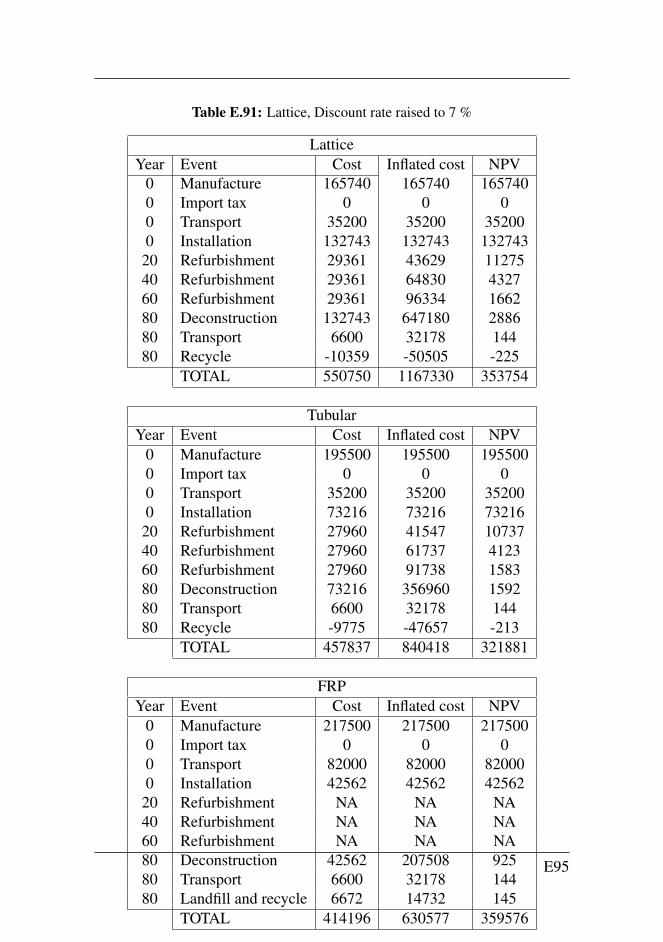
Table E.91: Lattice, Discount rate raised to 7 %
LatticeYear Event Cost Inflated cost NPV
0 Manufacture 165740 165740 1657400 Import tax 0 0 00 Transport 35200 35200 352000 Installation 132743 132743 132743
20 Refurbishment 29361 43629 1127540 Refurbishment 29361 64830 432760 Refurbishment 29361 96334 166280 Deconstruction 132743 647180 288680 Transport 6600 32178 14480 Recycle -10359 -50505 -225
TOTAL 550750 1167330 353754
TubularYear Event Cost Inflated cost NPV
0 Manufacture 195500 195500 1955000 Import tax 0 0 00 Transport 35200 35200 352000 Installation 73216 73216 73216
20 Refurbishment 27960 41547 1073740 Refurbishment 27960 61737 412360 Refurbishment 27960 91738 158380 Deconstruction 73216 356960 159280 Transport 6600 32178 14480 Recycle -9775 -47657 -213
TOTAL 457837 840418 321881
FRPYear Event Cost Inflated cost NPV
0 Manufacture 217500 217500 2175000 Import tax 0 0 00 Transport 82000 82000 820000 Installation 42562 42562 42562
20 Refurbishment NA NA NA40 Refurbishment NA NA NA60 Refurbishment NA NA NA80 Deconstruction 42562 207508 92580 Transport 6600 32178 14480 Landfill and recycle 6672 14732 145
TOTAL 414196 630577 359576
E95

Table E.91: Discount rate lowered to 3 %
LatticeYear Event Cost Inflated cost NPV0 Manufacture 165740 165740 1657400 Import tax 0 0 00 Transport 35200 35200 352000 Installation 132743 132743 13274320 Refurbishment 29361 43629 2415640 Refurbishment 29361 64830 1987460 Refurbishment 29361 96334 1635180 Deconstruction 132743 647180 6082080 Transport 6600 32178 302480 Recycle -10359 -50505 -4746
TOTAL 550750 1167330 453162
TubularYear Event Cost Inflated cost NPV0 Manufacture 195500 195500 1955000 Import tax 0 0 00 Transport 35200 35200 352000 Installation 73216 73216 7321620 Refurbishment 27960 41547 2300440 Refurbishment 27960 61737 1892660 Refurbishment 27960 91738 1557180 Deconstruction 73216 356960 3354680 Transport 6600 32178 302480 Recycle -9775 -47657 -4479
TOTAL 457837 840418 393508
FRPYear Event Cost Inflated cost NPV0 Manufacture 233800 233800 2338000 Import tax 0 0 00 Transport 82000 82000 820000 Installation 42562 42562 4256220 Refurbishment 0 0 040 Refurbishment 0 0 060 Refurbishment 0 0 080 Deconstruction 42562 207508 1950180 Transport 6600 32178 302480 Landfill and recycle 6672 32529 3057
TOTAL 414196 630577 383944
E96
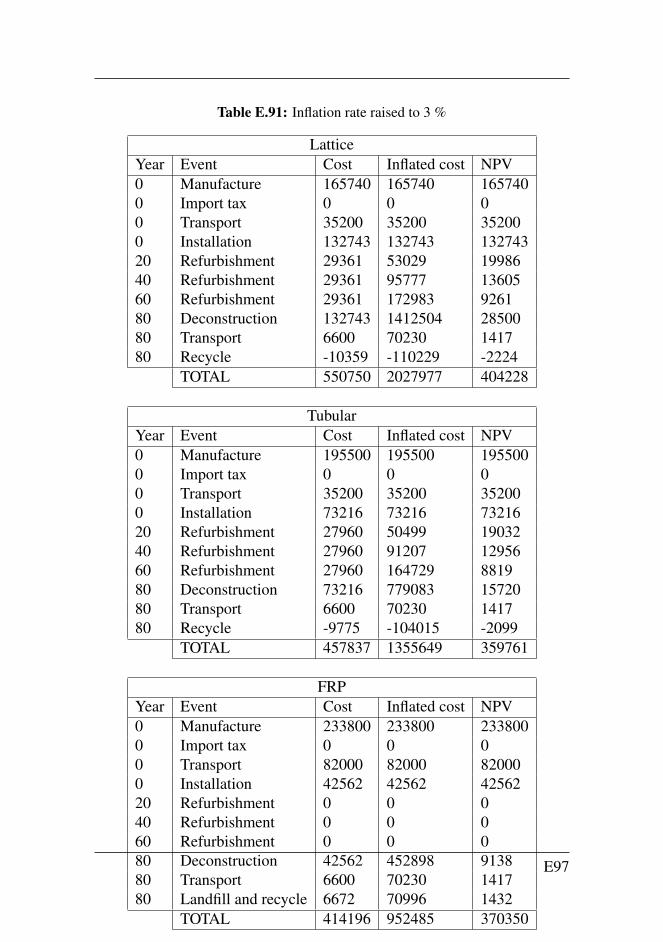
Table E.91: Inflation rate raised to 3 %
LatticeYear Event Cost Inflated cost NPV0 Manufacture 165740 165740 1657400 Import tax 0 0 00 Transport 35200 35200 352000 Installation 132743 132743 13274320 Refurbishment 29361 53029 1998640 Refurbishment 29361 95777 1360560 Refurbishment 29361 172983 926180 Deconstruction 132743 1412504 2850080 Transport 6600 70230 141780 Recycle -10359 -110229 -2224
TOTAL 550750 2027977 404228
TubularYear Event Cost Inflated cost NPV0 Manufacture 195500 195500 1955000 Import tax 0 0 00 Transport 35200 35200 352000 Installation 73216 73216 7321620 Refurbishment 27960 50499 1903240 Refurbishment 27960 91207 1295660 Refurbishment 27960 164729 881980 Deconstruction 73216 779083 1572080 Transport 6600 70230 141780 Recycle -9775 -104015 -2099
TOTAL 457837 1355649 359761
FRPYear Event Cost Inflated cost NPV0 Manufacture 233800 233800 2338000 Import tax 0 0 00 Transport 82000 82000 820000 Installation 42562 42562 4256220 Refurbishment 0 0 040 Refurbishment 0 0 060 Refurbishment 0 0 080 Deconstruction 42562 452898 913880 Transport 6600 70230 141780 Landfill and recycle 6672 70996 1432
TOTAL 414196 952485 370350
E97

Table E.91: Inflation rate lowered to 1 %
LatticeYear Event Cost Inflated cost NPV0 Manufacture 165740 165740 1657400 Import tax 0 0 00 Transport 35200 35200 352000 Installation 132743 132743 13274320 Refurbishment 29361 35826 1350240 Refurbishment 29361 43715 620960 Refurbishment 29361 53340 285680 Deconstruction 132743 294253 593780 Transport 6600 14630 29580 Recycle -10359 -22963 -463
TOTAL 550750 752484 362020
TubularYear Event Cost Inflated cost NPV0 Manufacture 195500 195500 1955000 Import tax 0 0 00 Transport 35200 35200 352000 Installation 73216 73216 7321620 Refurbishment 27960 34117 1285840 Refurbishment 27960 41629 591360 Refurbishment 27960 50795 271980 Deconstruction 73216 162299 327580 Transport 6600 14630 29580 Recycle -9775 -21668 -437
TOTAL 457837 585717 328539
FRPYear Event Cost Inflated cost NPV0 Manufacture 233800 233800 2338000 Import tax 0 0 00 Transport 82000 82000 820000 Installation 42562 42562 4256220 Refurbishment 0 0 040 Refurbishment 0 0 060 Refurbishment 0 0 080 Deconstruction 42562 94348 190480 Transport 6600 14630 29580 Landfill and recycle 6672 14790 298
TOTAL 414196 482130 360859
E98
Related Documents


