Design of spherical symmetric gradient index lenses …oa.upm.es/20930/1/INVE_MEM_2012_131141.pdf · Design of spherical symmetric gradient index lenses ... the Luneburg or the Eaton

Design of spherical symmetric gradient index lenses

Juan C. Miñano Dejan Grabovickic Pablo Benítez Juan C. González Asunción Santamaría

ABSTRACT

Spherical symmetric refractive index distributions also known as Gradient Index lenses such as the Maxwell-Fish-Eye (MFE), the Luneburg or the Eaton lenses have always played an important role in Optics. The recent development of the technique called Transformation Optics has renewed the interest in these gradient index lenses. For instance, Perfect Imaging within the Wave Optics framework has recently been proved using the MFE distribution. We review here the design problem of these lenses, classify them in two groups (Luneburg moveable-limits and fixed-limits type), and establish a new design techniques for each type of problem.

Keywords: Geometrical optics, GRIN lenses, spherical symmetric lenses, Maxwell Fish Eye, Luneburg lens, Eaton lens

1. INTRODUCTION

Spherical symmetric lenses made of isotropic gradient index media have always called the attention of optical designers. Today a renewed interest on these lenses has come from the analysis of the perfect imaging in the Wave Optics. Recently Leonhardt has proved the super-resolution properties of the Maxwell Fish Eye lens (MFE). This means that the MFE can produce images with details below the classic Abbe diffraction limit [1]. Unlike the negative refractive index perfect imaging devices [2], the MFE is a GRIN lens made of materials with a positive, isotropic refractive index distribution.

In this paper, we recall first the design procedure developed by Luneburg [3][4] and expanded by others [5], introducing the concept of angle of flight from which a function related to the refractive index distribution can be obtained by a linear integral transformation. This transformation allows us to derive old and new solutions for GRIN lenses just from linear combination of known lenses. In this way we will see, for instance, that the Eaton lens is just "twice" the Luneburg lens or that the MFE is the Eaton lens "minus" a homogeneous media lens.

Beside the analysis of the classical GRIN lenses (we will call them moveable-limits GRIN lenses), which are defined by the Abel integral equation, we present a numerical method for other GRIN lenses defined by the Abel integral equation with fixed limits (we will call them fixed-limits GRIN lenses). While in the case of the moveable-limits GRIN lenses, the only rays that pass through all the lens refractive layers are the ones with zero skew invariant, in the case of fixed-limits GRIN lenses this happens to all the rays. This makes a fundamental difference between the two types of the GRIN lenses. Fixed-limits GRIN lenses cannot be solved using classical Luneburg approach. This second type problem is mathematically equivalent to the constant (or prescribed) index core problem considered by Kotsidas et al. [6]. The procedure to solve the problem, if possible, is different.

Due to the spherical symmetry of the GRIN lenses, any ray trajectory is contained in a plane passing through the center of symmetry. This means, that we can restrict our discussion to ray trajectories in a plane defined by the polar coordinates (p, 9).

2. CONFORMAL TRANSFORMATION

In order to simplify the next explanations we are going to use a conformal transformation from the plane (p, 6) to the plane (x, y) given by

x = ln(A> y = 9 (1)

This is the conformal transformation defined by the natural logarithm complex analytical function (see for instance [3]).

Since the transformation is conformal, the ray trajectories in the plane (p, 9) with a refractive index distribution m(p) are transformed in curves of the plane (x, y) which are also rays if this plane has the refractive index distribution given by

n(x) = p m(p) (2)

The circle p=\ is transformed in the straight line x = 0. The points inside the circle p<\ are transformed in the half plane x < 0, while the points p > 1 are transformed in the half plane x > 0.

For instance, with this transformation, the Maxwell Fish Eye distribution mMFE(p)=2/(l + p2) transforms into the perfect image forming linear distribution wc(x)=l/cosh(x) [3].

3. STATEMENT OF THE DESIGN PROBLEM

We are going to consider the following design problem: Calculate the refractive index distribution m(p) of a lens either in the range 0 < p< 1 or in the range p>\, such that the rays impinging in the lens flight an angle inside it given by a function 9 (h), where h is the skew invariant of the ray. Figure 1 shows the definition of the angle of flight for two different cases of gradient index lenses, when the gradient index is in p <1, and when it is outside the unit circle. Lenses with gradient index in p< 1 are usually moveable-limits GRIN lenses, while in the other case we can find both moveable-limits and fixed-limits lenses .

arcos(ft)

Figure 1 Angle of flight 0(h) definition when the gradient index is in p<\ (left) and when it is in p>\ (right). White media has refractive index 1.

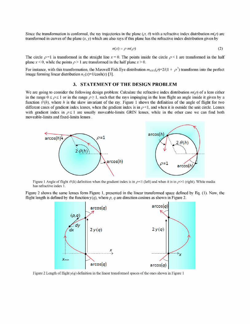
Figure 2 shows the same lenses form Figure 1, presented in the linear transformed space defined by Eq. (1). Now, the flight length is defined by the function y(q), where p, q are direction cosines as shown in Figure 2.

arcos(q)

2y(q)

arcos(q)

2y(q)

x

arcosfa) arcos(q)

Figure 2 Length of flight y(q) definition in the linear transformed spaces of the ones shown in Figure 1

4. MOVEABLE-LIMITS GRIN LENSES

Consider a ray trajectory from Figure 2. The elemental increment of the coordinate y is given as

q q dy = dx = sign(«) , = dx (3)

P(x) jn2(x)-q2

We are going to assume that the refractive index distribution is such that d[«2(x)]/dx > 0, for x < 0, and that the x coordinate of rays travelling find a minimum xmm beyond which they can't pass. By integrating the increment along the ray path inside the lens (for x<0) one gets

y(i) o

j dy= j sign(«)-= dx o *„,„(?) yjn2(x)-q2

S i g n ( w ) dx y(q) = q J -¡= 2(x)-q2

Note that n\xmin)=q2. Let's define the variables s, t and % as

n2 =\-t, sign(«)ife = dx = %dt

q2 = 1 - 5

Note that when sign(«)=l everywhere (positive refractive index everywhere) then x = x P m s a n additive constant. When there is a region with negative refractive index, then dx = ~dx. We are going to normalize the refractive index distribution to the one corresponding to x=0, «(0) or more precisely to H(0~) defined as

w((T) = lim«(x) (6) i -»0 i<0

Then, we can state that whenx —> 0~, n2 —> 1 and so / —> 0, and the integral of Eq. (4) can be written

s

f(s) = \-jZ=dt (7)

where

m=-*£0± (8)

Eq. (7) is a Fredholm integral equation of the first kind where x is the unknown function má y(q)=y((\-s)A) is known [7] [8]. This integral equation is usually called Abel integral equation. Luneburg was the first to notice that this kind of problems can be stated as an Abel integral equation. The integral at the right hand of Eq. (7) is proportional to the fractional integral operator of order Vi (noted by 72) applied on the function x- This operator is defined as (this is the Riemann fractional integral, which is one of many possible definitions of fractional integral) [8].

/*[*(,)] = _L \^P=dr (9)

Fractional integral operators Ia fulfill the semigroup property Ia7P = 7a+|3. This means, for instance, that applying twice the fractional integral operator/2 to the function x(t) we get/[x(/)] which is simply the integral of x(t)

rA \j% [*(/)]] =l[x(t)] = jx(T)dr (10)

Fractional derivatives are defined in a similar way as fractional integral. There is not a unique definition. The Caputo fractional derivative is the most adapted to our problem. Using Caputo's definition we can write Eq. (7) as

^¡7T = DlA(x(s)) (11)

Eq. (10) provides the key to solve the Abel integral. Applying again the fractional integral operator of order Vi, I 2 on both sides of Eq. (7) we get

-¡^Lds = \xdt = x(t)-X(0) (12)

Let's set ^(0)=0. Then

*® = ZI

z = --\- y(q)

H V ^ 2 - ' :dq

(13)

(14)

(15)

Assuming that we can evaluate Eq. (15) then we can plot x versus n2. Because we have set ^(/=0)=0, then ^(«2 = 1)=0. We have assumed that n2(x) is a non decreasing function in the domain x < 0. We can also plot ;¡f versus n, by assigning a negative refractive index when the dx ld(r?) < 0. Since dx= dx when the refractive index at x is positive and dx= ~dx in the opposite case, we can now plot ^versus x, and finally plot n(x). Hence, the calculation of refractive index distribution for a GRIN lens is done by the following steps:

1. Start with 0=f\(h). Note that the same function with different variables is the input data for the linear problem: y =fi (#)• We are assuming that n2(x) is a non decreasing function in the domain x < 0, i.e., I n(x) I ^ w(0~) which is set to 1 by definition. Then there is no ray with I q I > 1 that can enter into the half plane x < 0. Consequently the function y=f\(q) is only defined in the range \q\^ 1. Moreover, the function^ =f\(q) must be odd (fi(-q)= -fi(q)) thus we only need to know it in the range 0 ^ q ^ 1.

2. Calculate x=fi(n2) with Eq. (15). 3. Calculate x=fÁn) by assigning a negative refractive index where the derivative df2 Idn2 is negative. 4. Calculate z=fÁx) with the equations dx= dx (positive n) and dx= ~dx (negative n) with the contour condition

X= 0 whenx = 0. 5. Calculate n = n(x) with x =fi(n) a nd X =fÁx)-6. Use Eq. (1) and (2) to calculate m(p).

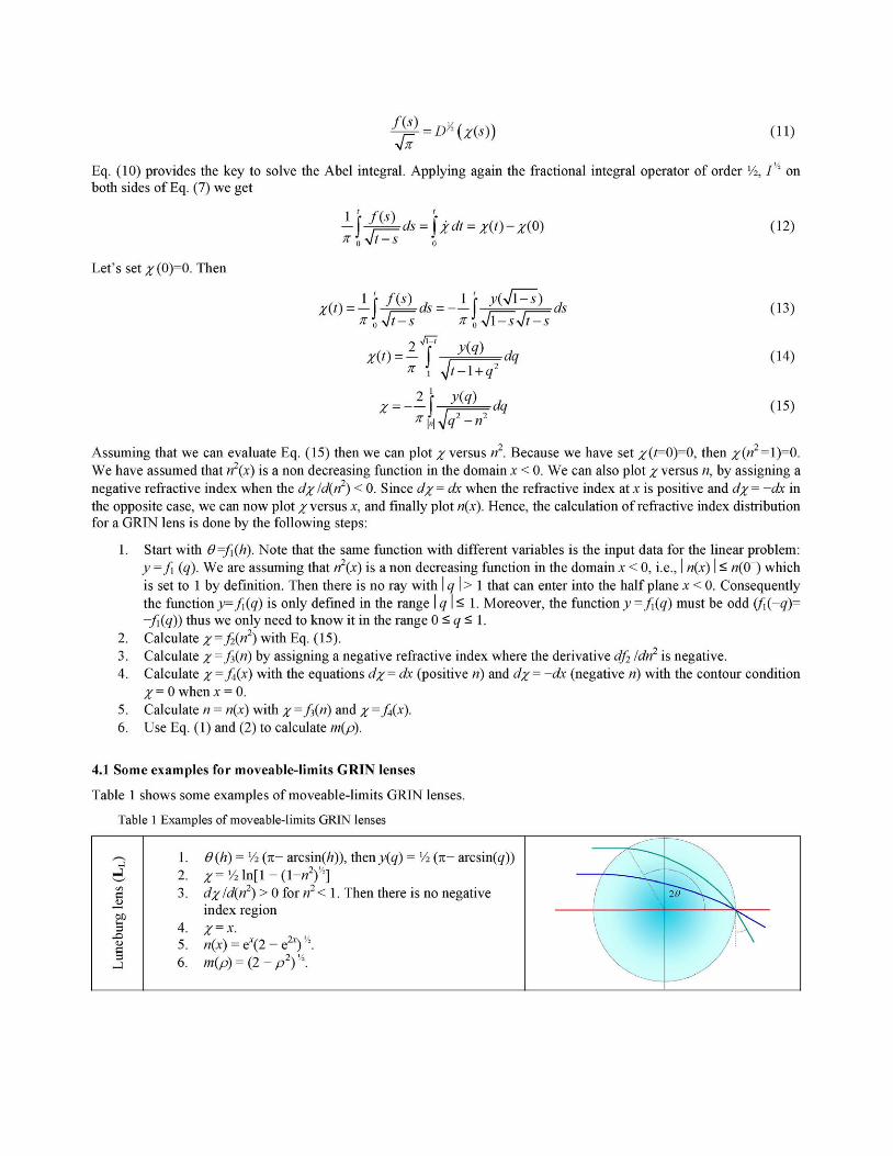
4.1 Some examples for moveable-limits GRIN lenses

Table 1 shows some examples of moveable-limits GRIN lenses.

Table 1 Examples of moveable-limits GRIN lenses

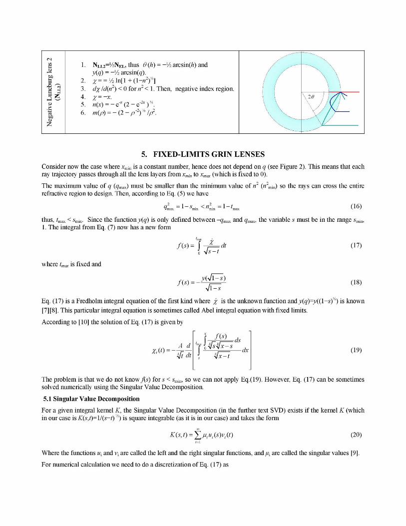
1. 0(h) =¥2 (TÍ- arcsin(/z)), thenX^) = ^ (n~ arcsin(^)) 2. ^=1 /2 ln[l-(l-«2)1 / 2] 3. dx ld(n2) > 0 for n2 < 1. Then there is no negative

index region 4. x = x. 5. n(x) = ex(2-e2x)y\ 6. m(p) = (2-p2)v\

¡

1. 0(h) = Till, and so _y(̂ ) = %I2. 2. z= ln[l - (1-w2)1*] " ln(«) = -AigCh(l/«) 3. dxld(n2) > 0 for n2 < 1. Then there is no negative

index region ¿J. y = j£

5. W(JC) = 2/( e-* + e*). 6. m(p) = 2/(l+p2)-

-

1. 6(h) = 7c-arcsin(//), then>(g) = 7u-arcsin(g). Since this is twice the angle of flight of the Luneburg lens and the fractional integral transform is linear, the corresponding %= fity2) must be twice that of the Luneburg lens, i.e, EL=2LL.

2. Z=\n{l-(l-n2f} 3. dxld(n2) > 0 for n2 < 1. Then there is no negative

index region 4. %=x. 5. n(x)= (2QX-Q2X)>/2.

6. m(p) = (2/p-\)>/2.

0 « o <u

8 1 O «¡

K

1. <9(/z) = arccos(/z), and so _y(̂ ) = arccos(g). This can also be written as _y(̂ ) = %/2 - arcsin(g), i.e. the difference of the angles of flight of the EL and MFE. We write HM = EL - MFE.

2. %= ln[l-(lV)' / 2] + ln(«) - ln[l+(lV)1/2]= V^n?) 3. d% /d(n2)>0 for n2<\. Then there is no negative

index region 4. %=x. 5. n(x) = ex. 6. m(p) = 1.

' i arccos(/7)

This is a lens with gradient index in p>\ , whose angle of flight is complementary to that of Eaton, so 6(h) = arcsin(/z), then y(q) = arcsin(g). M L -2(MFE -LL). Eq. (15) applies with a change of sign.

Z=\n[\+(\-n2f] dz ld(n2) < 0 for n2 < 1. Then there is no negative index region

X=x-n(x)= (2QX-Q2X)V\

m(p) = (2lp-l)V2mp>\

J0^*

f l

f f I 1

1 1 V \

^

i i

/ / j t / /

, ' - ^ ^

3

£

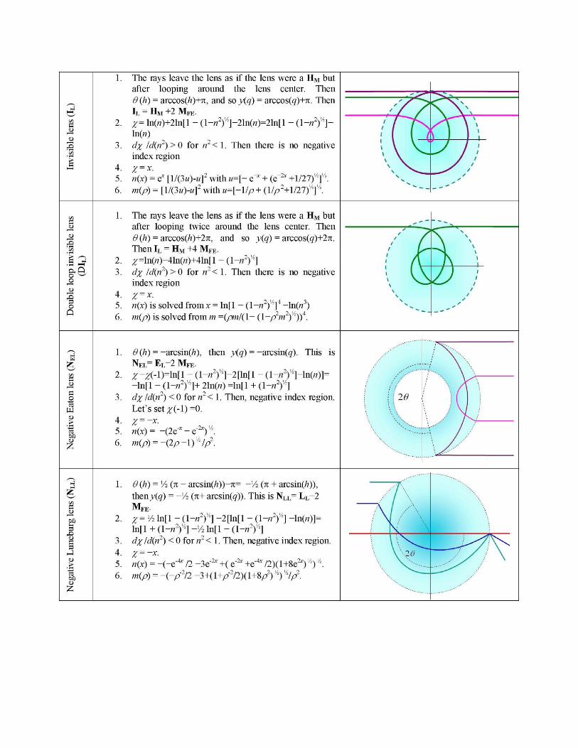
The rays leave the lens as if the lens were a HM but after looping around the lens center. Then 9(h) = arccos(/z)+7i, and so y(q) = arccos(g)+7i. Then IL = HM +2 MFE.

X= ln(«)+21n[l - (l-«2)'/2]-21n(«)=21n[l - (1-w2)14]-ln(w) d% ld(n2)>0 for n2< 1. Then there is no negative index region Z = x. n(x) = ex [\IQu)-uf with u=[- e~x + (e_2x +\l2lff. m(p) = [l/(3w)-w]2 with u=[-\lp+ (\lp2+\l2lff.

a <D

<D X> in

> ^ a j a Q o w

o <D

-S S3 O Q

2 3

4 5 6

The rays leave the lens as if the lens were a HM but after looping twice around the lens center. Then 6 (h) = arccos(/z)+27i, and so y(q) = arccos(g)+27i. Then IL = HM +4 MFE. ^=ln(«)-41n(«)+41n[l - (l-n2f] d% ld(n2)>0 for n2< 1. Then there is no negative index region

Z = *-«(x) is solved fromx = ln[l - (l-«2)2]4 -ln(«3) m(p) is solved from m =(pml(\- (l-p2m2)'A))4.

z

S3 Q

w

1

# (/?) = -arcsin(/z), then .y^) :

NEL= E L - 2 MFE. -arcsin(g). This is

2. z-Z(-l)=ln[l " (l-»2)/2]-2[ln[l - ( l -»yi- ln(»)]= -ln[l - (l-«2)'/2]+ 21n(w) =ln[l + (l-«2)'/2]

3. ¿^ ld(n2) < 0 for «2< 1. Then, negative index region.

4. 5. 6.

Let's set #(-l)=0. X=-X-n(x) = -(2ex - e-2x) '/2

/HC0) = - ( 2 / 7 - 1 ) ' / 2 / / 72

! ; 20

z

S3

s S3

<D

;¿ es bD

# (/?) = Vi (7i - arcsin(/z))-n= -!/2 (71 + arcsin(/z)), thenj^g) = -Vi (n+ arcsin(g)). This is NLL= L L - 2 MFE. X= Vi ln[l - (l-«2)'/2] -2[ln[l - (l-«2)'/2] -ln(w)]= ln[l + (l-«2)'/2] -Vi ln[l - (l-«2)'/2] d%ld(n2) < 0 for«2< 1. Then, negative index region.

X=-x-n(x) = -(-e"4x a -¿e2* +(e"2* +e"4x /2)(l+8e2x) '/2) '/2. w(p) : -(-/7"2/2 -3+(l+/?2/2)(l+8/?2),/2) '/2//32-

-Vi arcsin(/z) and N L L J ^ N E L , thus 0(h)-y(q) = -Vi arcsin(g). X= = Vi\xv\\+(\-n2f\ d% ld(n2) < O for n2 < 1. Then, negative index region. X=-x-n(x) = m(p)-

-Q2X)V\

-(2-p'Ylp2. ex (2 •

5. FIXED-LIMITS GRIN LENSES

Consider now the case where xmm is a constant number, hence does not depend on q (see Figure 2). This means that each ray trajectory passes through all the lens layers from xmin to xmax (which is fixed to 0).

The maximum value of q (gmax) must be smaller than the minimum value of n2 (n2mm) so the rays can cross the entire

refractive region to design. Then, according to Eq. (5) we have

l - 5 m „ < « „ mm mm

l-L (16)

thus, tmsx < smm. Since the function y(q) is only defined between -qmsx and qmsx, the variable s must be in the range sn

1. The integral from Eq. (7) now has a new form

/w=T X s-t

= dt (17)

where tmax is fixed and

As)-- (18)

Eq. (17) is a Fredholm integral equation of the first kind where % is the unknown function and y(q)=y((ls)2) is known

[7] [8]. This particular integral equation is sometimes called Abel integral equation with fixed limits.

According to [10] the solution of Eq. (17) is given by

X,(t): A d

tfi dt

f(s) rdS

x-s a. -dx

x-t (19)

The problem is that we do not know f(s) for s < smm, so we can not apply Eq.(19). However, Eq. (17) can be sometimes solved numerically using the Singular Value Decomposition.

5.1 Singular Value Decomposition

For a given integral kernel K, the Singular Value Decomposition (in the further text SVD) exists if the kernel K (which in our case is K(s,t)=\l(s-t) 2) is square integrable (as it is in our case) and takes the form

£(*,/) = | > , K , C S ) V , ( / ) (20)

Where the functions w¡ and v¡ are called the left and the right singular functions, and /¿¡ are called the singular values [9].

For numerical calculation we need to do a discretization of Eq. (17) as

( V

j - 1 ( A , - I ; V(Ay-D>

z /¡^í

ríft (21)

where Aj= /max#max, ymax being the number of terms in the sum of Eq. (21). The integrals from Eq. (21) can be calculated as

Í

/(*> = ! Í V

X

s-t

Now we sample values of s so Eq. (22) is given as

,dt * 2 £ i (A. (y - 0.5)) Us - A . (y -1) - ^ - Ajj ) (22)

/(A,. (/ - 0.5)) = 2 ¿ ¿(A, (y - 0.5)) ( J A , (/ - 0.5) - A . (j -1) - ^A, (/ - 0.5) - A .y ) = £ ¿(A, (y - 0.5))Z(/, j) (23)

where A1=(5max-5mm)/(/max-/mm+l), (imí¡x-imm+l) being the number of samples taken between smm and smax. The minimum value of /' in Eq. (23) is such that (/mm -1) A! < smm < imm A,. Since tmñX < smm then Ajymax < imm A,.

Using matrix and vector notation we have discrete form of Eq. (17)

i-O r̂ (w,i)

/ ;

y

Z(/,l)

M ' m i n ' . / ) ••• M'min > ./max)

£(U)

Z(z ,1) ... L(i , / ) ... Z(z , / ) v max ? J v max ? J J v max ? J max J

¿(Um a x)

max ? Jmax / /

Xi

\XJ^ J

(24)

Using discrete form of the SVD the matrix T from Eq. (24) takes the following form [9]

T=USVT (25)

Here, S is a diagonal matrix satisfying: S=diag (au a2,...an), and o¡ > a2>...>an>0. The matrices U and V consist of the left and right singular vectors, i.e. U=(ui, u2,..., u„) and V=(vi, v2,..., v„).

As an example, let's set /max=0.5, smax=i, smm=0.5. Figure 3 shows the left vectors for the kernel defined in Eq. (17). The right vectors have similar form, v1[/]=u1[«-/+l], / being a number \<l<n. According to [9] the solution of Eq.(24) is given as

(26)

However, this solution is called "naive" since there are extremely large errors coming from the noisy components related to the smaller singular values. When the Picard condition [9] is fulfilled, this noise can be decreased by truncating the sum in Eq. (26). The solution of Eq. (26) is obtained by retaining the first k components of the "naive" solution, k being

the number such that for all i<k the corresponding coefficients uf f , on average, decay faster than the cr..

x * = L — v ' ,=1 CT,

(27)

u

0.1

U S

g

•OH

D ?

•

^

1 1 :

"

J1"

: w

Figure 3 The left singular vector for the kernel defined in Eq. (17), number of samples is «=100.

5.2 Examples of fixed-limits GRIN lens

In order to explain the SVD method, let consider first the next problem, called Problem 1. For Eq. (17) let define the function^) as

/(*) = ( 4 ^ ) 2js-tmm (2^ + U

(28)

where tmsx=0.5. The true solution of this problem is known, %(t) = t. Let calculate this solution using the SVD method. After repeating the calculus given by Eq. (22)-(24) and doing the SVD for the matrix T, one gets the Picard plots as presented in Figure 4.

1E-12

l£.Ji

1E-S2

11 71

1E-92

1É-112

11 H i

1E-152

^ * * * ! : ^ : - w ^ .

1 20 40

V

\ \

• • - .

«0 SO 100

0.01

IE-OS

IE-10

16 1*

IE-IS

t

: . * •

• •

" • « : . .

• * 0 1 10 15 20

Figure 4 The Picard plot for Problem 1. The values of uff are presented in blue and the a, are presented in red (left).

Close up of the same Picard plot (right)

According to the graphs presented in Figure 4, it is clear that the coefficients uff decay faster than the cr. if i<9. If we

put k=9 in Eq. (27) we get a solution very close to the true one (see Figure 5). However, if we add more components, e.g. we put ¿=14, the solution start to oscillate introducing the noise as shown in Figure 5 .

0 5

0.«5

O.J

O.J5

0.1

D.H

0.1

o.:s

c.i

AM

0

0.1 0.2 O.J M 0.5

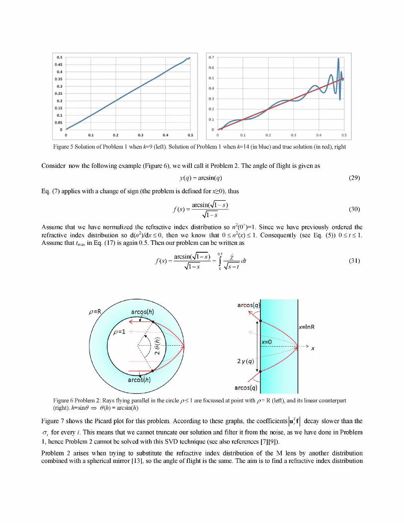
Figure 5 Solution of Problem 1 when k=9 (left). Solution of Problem 1 when k= 14 (in blue) and true solution (in red), right

Consider now the following example (Figure 6), we will call it Problem 2. The angle of flight is given as

y(q) = arcsin(g)

Eq. (7) applies with a change of sign (the problem is defined for x>0), thus

arcsin(Vl-5) f(s)-

n-s

(29)

(30)

Assume that we have normalized the refractive index distribution so n (0+)=l. Since we have previously ordered the refractive index distribution so d(«2)/dx<0, then we know that 0<«2(x)< 1. Consequently (see Eq. (5)) 0 < / < 1. Assume that imax in Eq. (17) is again 0.5. Then our problem can be written as

As)-arcsin(vl-5) X :dt (31)

arcos(q)

x=lnR

2y(q)

arcos(q)

Figure 6 Problem 2: Rays flying parallel in the circle p < 1 are focussed at point with p = R (left), and its linear counterpart (right). h=sin0 => 0(h) = arcsin(/!)

Figure 7 shows the Picard plot for this problem. According to these graphs, the coefficients uff decay slower than the

a, for every i. This means that we cannot truncate our solution and filter it from the noise, as we have done in Problem

1, hence Problem 2 cannot be solved with this SVD technique (see also references [7] [9]).

Problem 2 arises when trying to substitute the refractive index distribution of the M lens by another distribution combined with a spherical mirror [13], so the angle of flight is the same. The aim is to find a refractive index distribution

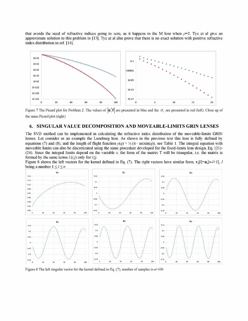
that avoids the need of refractive indices going to zero, as it happens in the M lens when p=2. Tyc et al give an approximate solution to this problem in [13]. Tyc at al also prove that there is no exact solution with positive refractive index distribution in ref [14].

1E-13

IE-12

1E-S2

1E-72

1E-92

1E11I

1E-1M

0 10

^ V _ \

\ _s 40 *o so too

0 1

1E-09

II l i

1E17 !0

Figure 7 The Picard plot for Problem 2. The values of uff are presented in blue and the a¡ are presented in red (left). Close up of

the same Picard plot (right)

6. SINGULAR VALUE DECOMPOSITION AND MOVE ABLE-LIMITS GRIN LENSES

The SVD method can be implemented in calculating the refractive index distribution of the moveable-limits GRIN lenses. Let consider as an example the Luneburg lens. As shown in the previous text this lens is fully defined by equations (7) and (8), and the length of flight function y(q) = Vi (n- arcsin(g)), see Table 1. The integral equation with moveable limits can also be discretizated using the same procedure developed for the fixed-limits lens design, Eq. (21)-(24). Since the integral limits depend on the variable s, the form of the matrix T will be triangular, i.e. the matrix is formed by the same terms L(ij) only for /'</'. Figure 8 shows the left vectors for the kernel defined in Eq. (7). The right vectors have similar form, v1[/]=u1[«-/+l], / being a number \<l<n

0,15

ÚLl

0.05

•

-0.05

•O.l

u,

, -- . .

• • .

\

\

„ » * ' * ' " *

/

0 » 4f f t «0 1 M

0.15

a i

OuM

0

- M í

-411 C

I I I

\

' • • * • •

2

; •

\ \

; '

\ / i 1 D 1 0 t

:

i i 0

V-L

0L«

9

- M í

4,1

4 »

C

u<.

A A r \ : 1 ** /

/ . \ . / \ /

\ / \ / \ / \j •-. : \\;

» • : : : r.p Kl) 1 c

Figure 8 The left singular vector for the kernel defined in Eq. (7), number of samples is «=100

Figure 9 shows the Picard plot for the Luneburg lens problem. According to these graphs, the coefficients uff decay

faster than the cr. for every i. This means that we are using all the members of the sum given in Eq. (27), i.e. k=n. This

arises from the fact that the Luneburg lens is a moveable-limits GRIN lens, defined by a well-posed integral equation, which was not the case for the design problems presented in the previous section.

10

1

0.1

0.01

.,

******** V

• .

0 20 40 60 80 100

Figure 9 The Picard plot for the Luneburg lens. The values of |uf f | are presented in blue and the a\ are presented in red

Figure 10 shows the solution of the problem. In the case of the Luneburg lens we have x(t) = -1/4(1-Ji)4i

0

-10

-20

-30

-40

-50

-60

-70

-80

-90

-100

r " ~ " - \ \ \

Figure 10 Solution for the Luneburg lens. True solution (in red) and the calculated solution (blue dots) for the function %(t)

7. CONCLUSIONS

In this paper the GRIN lenses design is organized in a new way. The GRIN lenses are divided into two groups, named moveable-limits GRIN lenses, which are defined by the Abel integral equation, and fixed-limits GRIN lenses (defined by the Abel integral equation with fixed limits). Due to convenience, both types are analyzed in a linear transformed space given by Eq. (1). For moveable-limits GRIN lenses, we show how old and new refractive index distributions can be obtained with linear combinations of existing ones.

Also we present a novel numerical design method for Fixed-limits GRIN lenses based on the Singular Value Decomposition. This method can be implemented in solving moveable-limits GRIN lenses, as well.

ACKNOWLEDGEMENTS

The authors thank the European Commission (SMETHODS: FP7-ICT-2009-7 Grant Agreement No. 288526, NGCPV: FP7-ENERGY.2011.1.1 Grant Agreement No. 283798), the Spanish Ministries (ENGINEERING METAMATERIALS: CSD2008-00066, DEFFIO: TEC2008-03773, ECOLUX: TSI-020100-2010-1131, SEM: TSI-020302-2010-65 SUPERRESOLUCION: TEC2011-24019, SIGMAMODULOS: IPT-2011-1441-920000, PMEL: IPT-2011-1212-920000), and UPM (Q090935C59) for the support given to the research activity of the UPM-Optics Engineering Group, making the present work possible.

REFERENCES

[1] Leonhardt, U., "Perfect imaging without negative refraction," New J. Phys. 11, 093040 (2009) [2] Pendry, J. B., "Negative Refraction makes a Perfect Lens", Phy. Review Let. 85, 3966-3989 (200) [3] Luneburg, R. K., [Mathematical Theory of Optics], University of California Press, Los Angeles (1964) [4] Cornbleet, S., [Microwave and Geometrical Optics], Academic (1994) [5] Sochacki, J., Flores, J. R., Gómez-Reino, C, "New method for designing the stigmatically imaging gradient

index lenses of spherical symmetry," Appl. Opt. 31, 5178-5183, (1992). [6] Kotsidas, P., Modi, V., Gordon, J., "Gradient-index lenses for near-ideal imaging and concentration with

realistic materials," Optics Express 19, 15584-15595, (2011) [7] Groetsch, C. W., "Integral equations of the first kind, inverse problems and regularization: a crash course," J.

Phys.: Conf. Ser. 73 012001 (2007) [8] Hermann, R., [Fractional calculus], World Scientific, Singapore (2011) [9] Hansen, P. C, [Discrete Inverse Problems: Insight and Algorithms], SIAM (2010) [10]Polyanin, A. D, and Manzhirov, A. V., [Handbook of Integral Equations], CRC Press, Boca Raton (1998) [ll]Kreyszig, E., [Differential Geometry], Dover, New York (1991) [12]Miñano, J. C, Benitez, P., Santamaría, A., "Hamilton-Jacobi equation in momentum space", Optics Express 14,

9083-9092, (2006) [13] Tyc, T., Sarbort, M., "Approximate magnifying perfect lens with positive refraction," arXiv:1010.3178v2

(2010) [14]Tyc, T.,Herzanova, L., Sarbort, M., Bering, K., "Absolute instruments and perfect imaging in geometrical

optics," New J. Phys. 13, 115004 (2011)