DESIGN OF SEPARATION UNITS USING SPREADSHEETS

(.3 ... 5111111§._c_l_a_s_s_r_o_o_m _________ )

DESIGN OF SEPARATION UNITS USING SPREADSHEETS

MARK A. BURNS, JAMES C. SUNG

University of Michigan • Ann Arbor, MI 48109-2136

M ost design calculations in an undergraduate sepa­rations course involve solving a combination of mass balance, mass transfer, and equilibrium equa­

tions. The resulting system of equations is usually not solved analytically for two reasons: 1) the system of equations is almost always nonlinear, and 2) some of the information (typically the equilibrium data) is not available in analytical form. Before the advent of digital computers, the only option available to teachers and students alike was to use graphical solution strategies. In recent years, however, the speed of computers has increased to such an extent that even lower­end personal computers have sufficient power to solve these design equations.

In choosing an application to solve the system of equa­tions, one must decide between faster, task-specific "separa­tions" programs (bought commercially, written in-house, or a combination of the twoY'1 and more general "equation solving" programs (e.g., Mathematica, Maple, HiQ, etc.).L21

The task-specific programs have the advantage that both the

Mark A. Burns received his BS in chemical engineering from the University of Notre Dame and his MS and PhD in chemical and biochemical engineering from the University of Pennsylvania. After spending several years teaching at the Uni­versity of Massachusetts, he joined the faculty at the University of Michigan. His research interests are in the area of bioseparations and include ad­sorption, chromatography, and micromachined systems.

-~--

James Sung just completed his second year of graduate work in chemical engineering at the Uni­versity of Virginia . He received his 8S from the University of Michigan in 1993. He is currently studying bacterial migration in porous media with applications to bioremediation.

input (the problems you choose) and the output (how the results are displayed) can be rather complex. The disadvan­tage is that the equations and the solution strategy are com­pletely transparent to the user. Equation-solving programs alleviate this problem but require that students learn what may be rather complex programs. Although each strategy has its advantages, we have chosen to use a simple equation­solving application to teach separation-unit design.

Although many programs can be used to solve systems of equations, we have chosen simple spreadsheet programs131

that can perform complicated mathematical calculations14·'1

and display the solutions in a variety of tabular and/or graphi­cal forms . The matrix-like structure of the spreadsheet is ideal for solving a system of coupled linear algebraic equa­tions using Gauss-Jordan EliminationL61 or simple matrix in­version. Other techniques can be used to solve more compli­cated nonlinear equations on spreadsheets, including sys­tems of both ordinary and partial differential equations.171

The limited power and speed of most spreadsheet applica­tions is more than compensated for by the ease of "program­ming" and the immediate presentation of results.

AN EXAMPLE: DISTILLATION

McCabe-Thiele and Ponchon-Savarit diagrams are the most common graphical solution strategies taught in a separations course. Realizing that this distillation-column design is merely the graphical solution of a series of sequential, nonlinear equations, one can construct a McCabe-Thiele diagram us­ing a spreadsheet. Assuming a total condenser is used, the distillate composition is equal to the vapor composition leav­ing the top tray. With the additional assumptions of constant relative volatility and constant molar overflow, the liquid composition leaving the top tray can be calculated using the equilibrium relationship. A mass balance on that tray then yields the vapor composition entering that tray from the tray

© Copyright ChE Division of ASEE 1996

62 Chemical Engineering Education

Before the advent of digital computers, the only option available to teachers and students alike was to use graphical solution strategies. In recent years, however, the

speed of computers has increased to such an extent that even lower-end personal computers have sufficient power to solve these design equations.

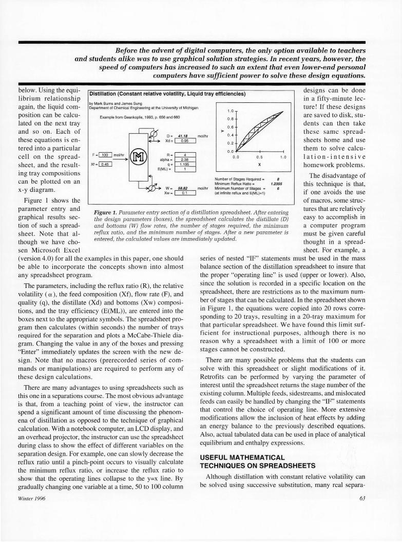
below. Using the equi­librium relationship again, the liquid com­position can be calcu­lated on the next tray and so on. Each of these equations is en­tered into a particul ar cell on the spread­sheet, and the result­ing tray compositions can be plotted on an x-y diagram.

Distillation (Constant relative volatility, Liquid tray efficiencies} designs can be done in a fifty- minute lec­ture! If these designs are saved to disk, stu­dents can then take these same spread­sheets home and use them to solve calcu-1 at ion - intensive homework problems.

by Mark Bums and James Sung Department of Chemical Engineering at the University of Michigan

1.0

Example from Geankoplis, 1993, p. 656 and 660 0 .8

0 .6 •

D = 41.18 mollhr 0 . 4

Xd= ! 0.95 !

A=~ alpha= 2.38 q= 1.195

E(ML)= 1

0 .2

0 .0

0 .0 0 .5

X

Number of Stages Required = Minimum Reflux Ratio =

1.0

8

W = 58.82 mol/hr Minimum Number of Stages = Xw = I 0.1 I (at Infinite reflux and E(ML)=l )

1.2355 6

The disadvantage of this technique is that, if one avoids the use of macros, some struc­tures that are relatively easy to accomplish in a computer program must be given careful thought in a spread-

Figure 1 shows the parameter entry and graphical results sec­tion of such a spread­sheet. Note that al­though we have cho­sen Microsoft Excel

Figure 1. Parameter entry section of a distillation spreadsheet. After entering the design parameters (boxes}, the spreadsheet calculates the distillate (DJ and bottoms (W) flow rates, the number of stages required, the minimum reflux ratio, and the minimum number of stages. After a new parameter is entered, the calculated values are immediately updated.

(version 4.0) for all the examples in thi s paper, one should be able to incorporate the concepts shown into almost any spreadsheet program.

The parameters, including the reflux ratio (R), the relative volatility (a), the feed composition (Xf), flow rate (F), and quality (q), the di stillate (Xd) and bottoms (Xw) composi­tions, and the tray efficiency (E(ML)), are entered into the boxes next to the appropriate symbols. The spreadsheet pro­gram then calculates (within seconds) the number of trays required for the separation and plots a McCabe-Thiele dia­gram. Changing the value in any of the boxes and pressing "Enter" immediately updates the screen with the new de­sign . Note that no macros (prerecorded series of com­mands or manipulations) are required to perform any of these design calculations.

There are many advantages to using spreadsheets such as thi s one in a separations course. The most obvious advantage is that, from a teaching point of view, the instructor can spend a significant amount of time di scussing the phenom­ena of distillation as opposed to the technique of graphical calculation. With a notebook computer, an LCD display, and an overhead projector, the instructor can use the spreadsheet during class to show the effect of different variables on the separation design. For example, one can slowly decrease the reflux ratio until a pinch-point occurs to visually calculate the minimum reflux ratio, or increase the reflux ratio to show that the operating lines collapse to the y=x line. By gradually changing one variable at a time, 50 to 100 column

Winter 1996

sheet. For example, a series of nested "IF" statements must be used in the mass balance section of the distillation spreadsheet to insure that the proper "operating line" is used (upper or lower). Also, since the solution is recorded in a specific location on the spreadsheet, there are restrictions as to the maximum num­ber of stages that can be calculated. In the spreadsheet shown in Figure 1, the equations were copied into 20 rows corre­sponding to 20 trays, resulting in a 20-tray maximum for that particu lar spreadsheet. We have found this limit suf­ficient for instructional purposes, although there is no reason why a spreadsheet with a limit of 100 or more stages cannot be constructed.

There are many possible problems that the students can solve with this spreadsheet or slight modifications of it. Retrofits can be performed by varying the parameter of interest until the spreadsheet returns the stage number of the existing column. Multiple feeds, sidestreams, and mislocated feeds can easily be handled by changing the "IF" statements that control the choice of operating line. More extensive modifications allow the inclusion of heat effects by adding an energy balance to the previously described equations. Also, actual tabulated data can be used in place of analytical equilibrium and enthalpy expressions.

USEFUL MATHEMATICAL TECHNIQUES ON SPREADSHEETS

Although distillation with constant relative volatility can be solved using successive substitution, many real separa-

63

tion systems have complexities that make their design on spreadsheets more complicated (see Table 1). Over the last several years, we have found that a number of mathematical techniques are useful in solving a wide variety of separation problems. They are listed below with a description of their implementation on a spreadsheet and an accompanying sepa­ration unit design problem.

tion was, say, y=0.355, linear interpolation between the y=0.304 and the y=0.418 data points would yield a value of x=0.078 for the liquid composition, or

Linear Interpolation and Lookup Tables (Distillation with Equilibrium Data)

X = Xbelow + (x above - Xbelow )(y- Ybelow )/(Yabove - Ybelow) (l)

This interpolation is performed in the spreadsheet by using lookup commands that return they values above and below the actual y value in the "data table" and the associated x values. The data points do not need to be evenly spaced to

The previous distiIJation spread­sheet assumed constant relative vola­tility (a) for the binary mixture. The vapor-liquid equilibrium of most bi­nary mixtures, however, is not ideal and is instead best represented by tabulated equilibrium data. The use of tabulated data as opposed to as­suming constant a is irrelevant when using graphical techniques but pre­sents a significant problem in most analytical solution strategies.

Distillation using the McCabe-Thiele method with equilibrium data points

by Mal1< Bums and James Sung Department of Chemical Engineering at the University of Michigan

··~ Example from King, 1980, 0 .8

p.251,Prob. 5-B D = 139.54 molhu 0 .6 ··-~ • 0 .4

(@) 0 . 2 •·rn F • CE] molhv • · 1 0 .0 - E{ML): 1 0 .0 0 .5 1 .0 xr - LILJ

X

w- 220."6 "'°"'' Xw= ~ Number of Stages Required • 16

EauiHbclum 0111 Enttx

Point No. X y

0 0.000 0.000 1 0.020 0.134 2 0.060 0.304 3 0.100 0.•18 4 0.200 0.579 5 0.300 0.665

• 0.400 0.729 7 0.500 o.n& • 0.600 0.825 9 0.700 0.870

10 O.!MlO 0.915 11 0.900 0.953 12 0.950 0.979 13 1.000 1.000 14 1.000 1.000

Using tabulated data in spread­sheets is quite simple due to the tabu­lar format of the spreadsheets. Once the equilibrium data is entered, in­terpolation between data points (a necessary operation when calculat­ing equilibrium values) can easily be accomplished using either cubic (or higher) spline fits or simple lin­ear interpolation. We have found that linear interpolation is preferred in almost all cases because (a) the cal­culations are extremely easy, (b) an increase in accuracy in one re-

Figure 2. Distillation spreadsheet using tabulated equilbrium data. Note that the data points do not need to be evenly spaced or fill the entire table (an extra (1 .0,1 .0) is added at the end of the table). Although spline fits can be used to interpolate the data , we have found that using simple linear interpolation gives the most accurate results provided a sufficient number of data points is used.

gion from a cubic spline fit is usually offset by a decrease in accuracy from an incorrect fit at another location, and (c) in a region of high curvature, ex-tra data points can be added to increase the accuracy of the linear fit.

As an example, consider the equilibrium data entered into the spreadsheet shown in Fig­ure 2. In "stepping down" a distillation column design, one might know the vapor compo­sition leaving a tray and want to calculate the liquid concen­tration in equilibrium with that value. If the vapor composi-

64

TABLE 1 Mathematical Techniques Used in Separation Spreadsheets

Separation System

General Countercurrent Unit design, linear equilibrium Unit design, nonlinear equilibrium Unit design , equilibrium data Retrofit, linear equilibrium Retrofit, nonlinear equilibrium Retrofit, equilibrium data

Specific Unit Design Ideal distillation Distillation with equilibrium data Distillation with equil./enthalpy data Absorption (real equilibrium data) Liquid/Liquid extraction (immiscible) Liquid/Liquid extraction (miscible)

Matrix Jacobian/ Manipulations Iteration

Successive Linear Substition Interpolation

Quadratic Fit

Numerical Integration

Chemical Engineering Education

perform these calculations and there is no set maximum number of points that can be used in the table.

Figure 2 also shows the earlier distillation spreadsheet modified to include equilibrium data and lookup commands. Although 13 data points are shown in the example (the 14th is a repeat) , the table can be expanded to include 100 or more points. For di splay purposes (and for most calculations), the 14 points produce a relatively smooth curve. Note that, for low x-values where the slope of the equilibrium curve is large, additional data points have been added. Also, several columns between "x" and "y" data columns are hidden that shift the x- and y-values up one row; this technique makes interpolation with lookup commands much simpler.

Matrix Inversion (Countercurrent Distribution)

For the design of countercurrent separation systems, suc­cessive substitution is needed because the number of stages that will be used in the system is unknown. If the design involves a known number of stages (e.g., retrofitting a sepa­ration to an existing column), then matrix techniques can be used instead. Most spreadsheets include basic matrix-ma­nipulation commands such as matrix inversion and multipli­cation. Although other techniques can be used to solve the

equations, the simplicity and speed of matrix manipulations on spreadsheets makes matrix techniques particularly attrac­tive.

As an example, one can calculate the separation that would be obtained for a countercurrent distribution system (such as immiscible liquid-liquid extraction). If the equilibrium dis­tribution coefficient is constant (linear equilibrium relation­ship) and the number of stages is fixed, the mass balance equations reduce to a set of linear algebraic equations. Once the flow rates and compositions of the entering streams are specified along with the equilibrium constant (K=y/x), the equations for a 5-stage system are

- (L + KV)X 1 + (KY )X 2 =LX (2) ,n

LX 1 -(L + KY)X2 + (KY)X3 =0 (3)

LX 2 - (L + KV)X3 + (KY)X4 =0 (4)

LX3 -(L + KV)X 4 + (KV)XOUI =0 (5)

LX4 -(L + KV)XOU( = -Yin V (6)

where X and L are the composition and flow rate of one liquid, and Y and V are the composition and flow rate of the

Countercurrent or Cocurrent Distribution (Line~ar_E_q..:.u_l_lib_r_iu_m--'-) - ----~ by Mark Burns and James Sung

other. Figure 3(a) shows the flow diagram for the process.

Department of Chemical Engineering at the University of Michigan

Counter- (1) or Co- (0) current operation ?

Xln = 0.001 Yin = 0.01

K = 2.53 (y= Kx)

0.002

X

0.004

Yout 0.0057

n ft N n ~

<---... ••u••>

Xln 0.0010

0.0076 0.0087 0.0094 0.0098 0.01

EQ ~=; ~ ~=::~- SJ =:.:· SJ -~->- ~ ==~ X1 X2 X3 X4 Xout

0.0023 0.0030 0.0034 0.0037 0.0039

L= 1 · ·-~> I

Figure 3 ( a) (above) Data en try section for staged countercurren t or cocurren t separation assuming linear equilibrium and immiscible phases (liquid-liquid extraction, absorption , adsorption, etc.). (b) (below) Matrix calculation section of spreadsheet.

Solution using matrix lnvarslon Eauati9os In Matrix Notatiorr Coefficient Matrix

-241.80 90.00

151.80 -241.80

90.00 0

0 0

Inverted Coefflclcn Ma rix -0.006382 -0.006036 -0.003579 -0.009614 -0.001916 -0.005148 -0.00093 1 -0.002501 -0.000346 -0.000931

Solution Y1 0.00571 Y2 0.00759 Y3 0.00871 Y4 0.00937 VS 0.00977

Winter 1996

IAl

0 151.80

-241.80 90.00

0

'A Inverse\ -0.005451 -0.008684

-0. 0106 -0.005148 -0.0019 16

0 0 0 0

151.80 0 -241.80 151.80

90.00 -241.80

-a.004466 -a.002804 -a.007114 -0.004466 -0.008684 -a.005451 -a.009614 -0.006036 -a.003579 -a.006382

x,. 0.00226 X2- 0.00300 Xh 0.00344 X4- 0.00371 XS. 0.00386

'•' x, X2 X3 X4 XS

S~ution Scheme (1) Ax • b (2) x = A_lnverse•b (3) Y= Kx

b -0.09 0.00 0.00 0.00

The equations above can also be written in matrix notation:

AX= b (7)

To solve for X, the matrix A is first inverted

using the matrix inversion command. The ma­trix multiplication command is then used to find the product of the inverted matrix and the vector b or

(8)

The composition of the other stream (Y ) is found by merely multiplying X by the equilibrium con­stant, or

Y=KX (9)

~

The section of the spreadsheet that performs these calculations is shown in Figure 3(b ). The coefficients of the above equations are entered into the matrix ~ . Calculations are performed

each time a new flow rate, equilib­rium constant, or composition is en­tered into the spreadsheet. For nonlin­ear equilibrium relationships, a simi­lar spreadsheet can be constructed ex­cept that an iterative scheme is neces­sary (Newton's method, multi variable:

65

Yin

L =~ f I dy C Kya (1-y)2 en[l-y *]

Yout 1-y

(13)

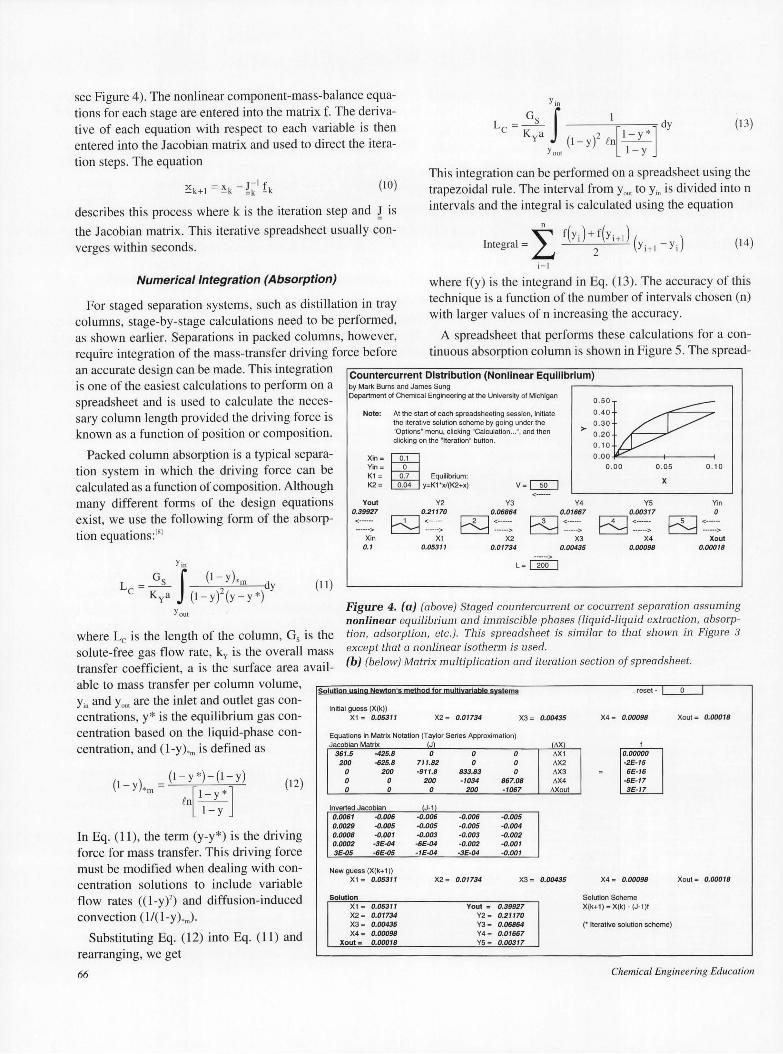
see Figure 4). The nonlinear component-mass-balance equa­tions for each stage are entered into the matrix f. The deriva­tive of each equation with respect to each variable is then entered into the Jacobian matrix and used to direct the itera­tion steps. The equation

(10)

describes this process where k is the iteration step and J is

the Jacobian matrix. This iterative spreadsheet usually con­verges within seconds.

This integration can be performed on a spreadsheet using the trapezoidal rule. The interval from y0 " 1 to Y;" is divided into n intervals and the integral is calculated using the equation

n

L f(y)+f(y 1)( ) Integral= 1 t+ y. -y .

2 t+I , (14)

i=I

Numerical Integration (Absorption)

For staged separation systems, such as distillation in tray columns, stage-by-stage calculations need to be performed, as shown earlier. Separations in packed columns, however, require integration of the mass-transfer driving force before

where f(y) is the integrand in Eq. (13). The accuracy of this technique is a function of the number of intervals chosen (n) with larger values of n increasing the accuracy.

A spreadsheet that performs these calculations for a con­tinuous absorption column is shown in Figure 5. The spread-

an accurate design can be made. This integration is one of the easiest calculations to perform on a spreadsheet and is used to calculate the neces­sary column length provided the driving force is known as a function of position or composition.

Countercurrent Distribution (Nonlinear Equilibrium) by Mark Bums and James Sung ,-------------~

Packed column absorption is a typical separa­tion system in which the driving force can be calculated as a function of composition. Although many different forms of the design equations exist, we use the following form of the absorp­tion equations: 181

Yin

C 2 y (11)

Department of Chemical Engineering at the University of Michigan

Note:

Xin= Yin= K1 = K2 =

Yout 0.39927

······> Xin

0.1

At the start of each spreadsheeting session, initiate the iterative solution scheme by going under the "Options" menu, clicking "Calculatlon ... ", and then clicking on the "Iteration" button.

Equilibrium: y=K1 "x/(K2+x)

•

Y2 Y3 Y4

~ot~~o 8Jo::~? ~o~~:'.-~~7 X1 X2 X3

0.05311 0.01734 0.00435

0 .50~ 0 .40

0.30

0 .20

0.10

0.00

0 .00 0.05

X

0.10

YS Yin

~0;~~~7 EQ ~:::_;~ X4 Xout

0.00098 0.00018

L =~ f (1-y).m ct Kya (1-y) (y-y *)

Yout

where Le is the length of the column, Gs is the solute-free gas flow rate, kv is the overall mass transfer coefficient, a is the surface area avail-

Figure 4. (a) (above) Staged countercurrent or cocurrent separation assuming nonlinear equilibrium and immiscible phases (liquid-liquid extraction, absorp­tion, adsorption, etc.). This spreadsheet is similar to that shown in Figure 3 except that a nonlinear isotherm is used.

able to mass transfer per column volume, Y;" and y

0"' are the inlet and outlet gas con­

centrations, y* is the equilibrium gas con­centration based on the liquid-phase con­centration, and (1-y).'" is defined as

(1-y*)-(1-y) (l-y). m= [1- *] J!n __ Y_

1-y

(12)

In Eq. (11), the term (y-y*) is the driving force for mass transfer. This driving force must be modified when dealing with con­centration solutions to include variable flow rates ((l-y)2) and diffusion-induced convection (1/(1-y).m).

Substituting Eq. (12) into Eq. (11) and rearranging, we get

66

(b) (below) Matrix multiplication and iteration section of spreadsheet.

Solution using Newton's method for multivariable systems

Initial guess (X(k)) X1 = 0.05311 X2 = 0.01734 X3= 0.00435

Equations in Matrix Notation (Taylor Series Approximation) Jacobian Matrix t J\

361.5 -425.8 0 0 O 200 -625.8 711.82 0 O

0 0 0

200

Inverted Jacobian 0.0061 -0.006 0.0029 -0.005 0.0008 -0.001 0.0002 ·3E-04 3E-05 ·6E·05

New guess (X(k+ 1 )) X1 = 0.05311

Solution X1 = 0.05311 X2 = 0.01734 X3= 0.00435 X4= 0.00098

Xout = 0.00018

-911.8 200

0

IJ-1\ -0.006 -0.005 -0.003 -6E-04 -1E-04

X2=

833.83 0 -1034 867.08

200 -1067

-0.006 ·0.005 -0.005 ·0.004 -0.003 ·0.002 -0.002 -0.001 -3E-04 -0.001

0.01734 X3=

Yout = 0.39927 Y2= 0.21170 Y3= 0.06864 Y4= 0.01667 YS= 0.00317

(Li)(\

AX1 AX2 AX3 AX4

AXout

0.00435

reset- I

X4 = 0.00098

X4 =

0.00000 -2E-15 6E-16

-6E-17 3E-17

0.00098

Solution Scheme X(k+1) = X(k) - (J-1)1

(• Iterative solution scheme)

o I

Xout = 0.00018

Xout= 0.00018

Chemical Engineering Education

sheet uses tabulated equilibrium data and calculates the driv­ing force at 20 points along the column (usually sufficient although more can be added). The trapezoidal rule is then used to calculate the integral listed above, and the length of column necessary to perform the separation in either a co- or countercurrent configuration is di splayed. Note that the in­tegral calculations in the spreadsheet are concealed in­side the diagram of the column (see Figure 6). Also, in thi s spreadsheet, the outlet gas-phase concentration is specified ; a similar spreadsheet can be developed speci­fying the outlet liquid concentration.

interpolations are not easily found . Using equations instead of data eliminates this problem but requires the user to generate and enter the equations into the spreadsheet.

An easier technique involves programming the spread­sheet to generate a least-squares quadratic polynomial to fit the data and then use the equation to design the separation system. The least-squares quadratic polynomial is defined as that polynomial , p(x), that minimizes the sum of the squares of the error between the polynomial and the data points, (x,, fJ The function to be minimized can be represented by

n

Quadratic Fits (Liquid-Liquid Extraction)

The solutions presented thus far have involved relatively simple mathematical techniques. If these techniques were applied to liquid-liquid extraction with partially miscible phases or di stillation with tabulated enthalpy data, difficul­ties wou ld arise. Specifically, stagewise calculations are dif­ficult when the stepping procedure occurs on graphs with multiple "tabulated data" lines because the endpoints of the

Q(f,P)= I,[f; - P{x;)j2 (15)

i = I

where the quadratic polynomial is

P(x) = a1x2 + a2x + a3 (16)

Absorption in Packed Columns (Countercurrent, gas exit specified) by Mark Bums and James Sung

The coefficients a1, a2, and a3 are then fou nd by taking the derivative of Q with respect to each coefficient and setting these equations equal to zero, thus minimizing the function

Q. After considerable mathematical manipula­tions ,191 the coefficients can be shown to be

Department of Chemical Engineering at the University of Michigan

Liquid In 40.80 mol/hr'ft2

O molfrac

Gs= 27.69 mol/hr0 ft2

Ls= 40.80 mol/hr0 ft2

Liquid out 43.2 mo11t1r·tt2 0.06 molfrac

I A I I I I I I I I V I

Gas out 27.77 0.003

Flow rates ente~ln : Gas = 30.18 mol/hr 0 ft2

mol/hr0 ft2 Liquid = 40.80 mol/hr 0 ft2

Columl setup: I Kya = 27.60 mol/hr0 tt3

Counter(" or ~o(O}I molfrac

Compositions enterln : Composition lea~ Gas= 0 .083 mol frac Gas= ~mol frac

Liquid = 0.000 mol frac Liquid= 0.056 mol frac Length:: 11.12 ft

Example from Welty , et al, 1984, p. 693

Gas in 30.18 mol/hr0 ft2 0.083 mol frac

• ::::1~ 0 .00 ~ I

0.00 0 .02 0 .0 4 0 .06 0 .08

X

Figure 5. Continuous packed column absorption spreadsheet. After entering the parameters, the spreadsheet calculates (using Eq. 13) the length of packed column necessary to pe1form the desired separation . Note that, although we have specified the exiting gas composition, a similar spreadsheet can be devleoped that uses a specified exiting liquid composition.

Ls- 408 -I J, Gs= 27.69

where

I {, Id In Position X X I v• I 11( ... l I NeQative? I J I y V Gas Liqu out 0 mol/hr•tt2 0 0.0000 0.0000 0.0000 334.84 FALSE 0.0030 0.0030 27. 40.8 77

molfrac 0.05 0.0029 0.0029 0.0037 284.11 FALSE 1.33 0.0074 0.0073 0.00 0 3 0 .1 0.0059 0.0059 0.0075 247.92 FALSE 2.47 0.0117 0.0116

0 .15 0.0088 0.0088 0.0112 220.84 FALSE 3.46 0.0160 0.0158 0.2 0.0117 0.0118 0.0149 199.84 FALSE 4.34 0.0204 0.0200

Gs= I 0.25 0.0145 0.0147 0.0185 183.08 FALSE 5.13 0.0247 0.0241 A 9 mol/hr*ft2 I 0.3 0.0174 0.0177 0.0221 168.09 FALSE 5.86 0.0291 0.0283 I Leng 27.6 th=

I 0 .35 0.0202 0.0206 0.0256 154.37 FALSE 6.52 0.0334 0.0323 I 11.1 2 I 0.4 0.0230 0.0236 0.0291 143.09 FALSE 7.12 0.0378 0.0364 I

0 mol/hr*ft2 I 0 .45 0.0259 0.0265 0.0323 129.08 FALSE 7.67 0.0421 0.0404 I Exa 40.8 mplef1 V 0 .5 0.0286 0.0295 0.0351 113.65 FALSE 8.15 0.0465 0.0444 I 1984 ' p. 6!

0.55 0.0314 0.0324 0.0380 101.78 FALSE 857 0.0508 0.0484 0.6 0.0342 0.0354 0.0<08 92.38 FALSE 8.95 0.0552 0.0523

Id out 0.8 0.0451 0.0472 0.0519 68.60 FALSE 10.17 0.0725 0.0676 Gas 2 mol/hr*ft2 0.85 0.0477 0.0501 0.0545 64.47 FALSE 10.42 0.0769 0.0714 30. 1 6 molfrac 0 .9 0.0504 0.0531 0.0572 60.89 FALSE 10.66 0.0812 0.0751 0.08

1' I 0.95 0.0531 0.0560 0.0598 57.76 FALSE 10.88 0.0856 0.0788 11' I 1 0.0557 0.0590 0.0625 55.00 FALSE 11.08 0.0899 0.0825

Figure 6. View of the hidden columns in the absorption spreadsheet shown in Figure 5.

Winter 1996

(! 7)

·+:l xi x2

I ?

X2 x-~= 2

X x2 n n

!{1 Thus, the coefficients (.g_) are fou nd from the data (f) using the matrix x .

Figure 7 shows the implemen­tation of this technique on a spreadsheet that calculates the number of stages necessary for a particular liquid-liquid extrac­tion system. The coefficients of the calcu lated equation are shown in Figure 8 and can be

67

used throughout the spreadsheet in place of the data to calcu­late the required number of stages. If the fit obtained by this method is unsatisfactory, additional data points can be added to improve the fit or a higher order curve can be used. In our work, we have found that quadratic fits do remarkably well for both liquid-liquid extraction and enthalpy data in distillation.

CONCLUSIONS

What spreadsheets lack in power, they make up for in ease of use. For a student, the results of changes to design vari­

spreadsheets as well as perfecting a number of the others. Wilbur Woo investigated the use of cubic splines (which we found were not necessary) and constructed the original "data" spreadsheets. Mike Johns followed Professor Frey's paper and did some simple chromatography solutions. Mike Vyvoda spent considerable time debugging the final versions and writing the all-important nomenclature tables. In addition to these students, many other undergraduates at the University of Michigan contributed to the spreadsheets through feed­back in our separations course.

ables in separation spreadsheets can be seen in a few seconds in tabular or graphical form. In addition to changing design variables, the stu­dent can also change the structure of the spread­sheet to design more complicated separation units.

Countercurrent Liquid/Liquid Extraction by Mark Burns and James Sung Department of Chemical Engineering at the University of Michigan

~ 1 .

For instance, in binary di stillation, multiple feeds, Extract

V1

Feed ;. 1.6

~ 1.4

1000.00 Lo ~ 1.2

one or more sidestreams, or mislocated feeds Ac:~:,ckl can all be added to the basic spreadsheet. The lsopropyl elher

techniques used to solve systems of equations in

1818.52 0.1564 0.0403 0.8034

0.3500 Acetic Acid 0.6500 Water 0.0000 lsopropyl ether

Example from Wankat,

> 1 .0 .; 0.8 ;.

0 .6 C

0 .4 .. 0.2 )(

these spreadsheets can also be applied to other problems in other courses.

Vn+1 Acetic Acid

Water lsopropyl ether

Solvent

1475.00 0 .0000 0.0000 1.0000

1988, p. 595

Raffinate

656.48

~ 0.8786 0.0214

Ln Acetic Acid

Water lsopropyt ether

-0 . 5 0.0 0.5 1 .0

Xsolute,Ysolute

Number of Stages Required= 6

Note: Spreadsheet may generate incorrect solutions when attempting a separation near the lait oint

Figure 7. Parameter entry and graphical output section of the liquid/liquid extraction spreadsheet. This spreadsheet is particularly complex because "step­ping" between the equilibrium curves with linear interpolation is difficult. But using a quadratic fit to the data allows easy calculation of the required number of stages for any given system.

For an instructor, separation spreadsheets en­able the lecturer to focus on the principles be­hind the separation processes instead of the te­dious solution procedures. But care must be taken to ensure that the students do not use the spread­sheets to solve homework problems that, with the aid of the spreadsheets, are merely "plug­and-chug." During the separations course at Michigan, each spreadsheet is typically in­troduced in lecture when that separation unit Petermloe Quadratic Le11t Squares EH for the Eoullibrtum Phase Pata

is first discussed. Homework problems then include both simple, plug-and-chug type problems that require a single use of the spreadsheet and more complicated, multiuse problems (e.g., plot the number of trays needed to perform this distillation as a func­tion of reflux ratio).

Qualitative homework questions are also common. More difficult problems that re­quire the student to redesign the spreadsheet are sometimes used, but are typically reserved for group projects. Overall, the students have had a very favorable reaction to the introduc­tion of these spreadsheets in the separation course. As a final note, all the spreadsheets shown here are available from the authors. 131

ACKNOWLEDGMENTS

Many students were involved in develop­ing the spreadsheets shown in this paper. James worked on the original versions of the countercurrent distribution and distillation

68

SolvenVExtract Laver

X=

XT=

•=

Ra

X=

XT=

·-

1 -0.990

1 -0.990 0.980

0.4868 0.0627

-0.4339

ffinate la"er 1 1 1 1 1 1 1 1 1 1

-0.010 0.000

-0.0730 ~ .8146

...33.8160

-0.989 -0.971 -0.847 -0.715 -0.487 -0.165 -0.165 -0.165 -0.165

1 -0.989 0.978

a._3 a_2 ._,

-0.010 -0.012 -0.016 -0.023 -0.034 -0.106 -0.165 -0.165 -0.165 -0.165

-0.012 0.000

a_6 a_S a_4

0.980 0.978 0.943 0.717 0.511 0.237 0.027 0.027 0.027 0.027

1 1 -0.971 -0.847 0.943 0.717

0.000 0.000 0.000 0.001 0.001 0.011 0.027 0.027 0.027 0.027

1 1 -0.016 -0.023 0.000 0.001

0.000 0.004 0.019 0.114

f= 0.216 0.362 0.464 0.464

1 1 1 1 1 1 -0.715 •0.487 •0.165 -0.165 -0.165 -0.165 0.511 0.237 0.027 0.027 0.027 0.027

0.000 0.007 0.029 0.133

f= 0.255 0.443 0.464 0.464 0.464 0.464

-0.034 -0.106 -0.165 -0.165 -0.165 -0.165 0.001 0.011 0.027 0.027 0.027 0.027

Figure 8. Calculation of the quadratic equations used in the Figure 7 spreadsheet.

Chemical Engineering Education

REFERENCES 1. Jolls, K.R. , M. Nelson, and D. Lumba, "Teaching Staged­

Process Design Through Interactive Computer Graphics," Chem. Eng. Ed. , 28(2), 110 (1994)

2. Taylor, R., and K. Atherley, "Chemical Engineering with Maple," Chem. Eng. Ed. , 29(1), 56 (1995)

3. All the spreadsheets shown in this paper are available from the author. For copies of the spreadsheets, send a Macintosh or IBM compatible disk (state which one) and a stamped, self-addressed envelope to Mark A. Burns, Department of Chemical Engineering, University of Michigan, Ann Arbor, MI 48109-2136

4. Arganbright, D. , Mathematical Applications of Electronic Spreadsheets, McGraw-Hill Book Co., New York, NY (1985)

5. Rosen, E .M., and R.N. Adams, "A Review of Spreadsheet Usage in Chemical Engineering Applications," Comput. Chem. Eng., 11(6), 723 (1987)

6. Burns, M.A. , "Mass and Energy Balance on Microbial Pro­cesses," in Chemical Engineering Problems in Biotechnol­ogy, M.L. Shuler, Ed., AIChE, New York, NY (1989)

7. Frey, D.D., "Numerical Simulation ofMulticomponent Chro­matography Using Spreadsheets," Chem. Eng. Ed., 24(4), 204 (1990)

8. Geankoplis, C.J. , Transport Processes and Unit Operations, 3rd ed., Prentice Hall, Englewood, NJ (1983). Equation simi­lar to 10.6-16

9. Yakowitz, S. , and F. Szidarovszky, Introduction to Numeri­cal Computations, Macmillan Publishing Company, New York, NY (1989) 0

(.a_..51111113._b_o_o_k_re_ v_ie_w ______ __.)

CHEMICAL THERMODYNAMICS: BASIC THEORY AND METHODS, 5th ed. by Irving M. Klotz, Robert M . Rosenberg Published by John Wiley and Sons, Inc. , NY; 533 pages, $54.95 (hard cover) (1994)

Reviewed by Pablo G. Debenedetti Princeton University

The fifth edition of Klotz and Rosenberg's Chemical Ther­modynamics is similar in spirit to its four predecessors. It is a text on classical thermodynamics and its applications to mixtures , chemical reactions, and other situations of interest to chemists. It can be used both for undergraduate and gradu­ate instruction and requires no previous knowledge of ther­modynamics. The simple mathematical tool s needed to un­derstand the material are explained in the book.

The twenty-three chapters cover a wide range of topics. Following two introductory chapters on the history and ob­jectives of classical thermodynamics and on mathematical prolegomena, the First Law and its applications to chemical reactions and to the behavior of gases is discussed. Three chapters are also devoted to the Second Law, its consequences (reversibility, spontaneity, free energy functions) and its appli­cation to simple cases of phase equilibria (e.g, the Clapeyron equation, temperature dependence of enthalpies of transition).

Winter 1996

Other chapters discuss the Third Law, reaction equilibria, systems of variable composition, gas mixtures, the phase rule, ideal solutions, dilute solutions, activities in non-elec­trolyte solutions, the calculation of partial molar quantities from experimental data, the determination of activities of non-electrolytes, electrolyte solutions, free energy changes in solutions, gravitational fields, and the estimation of ther­modynamic quantities. The fifth edition also contains a new chapter on simple analytical and numerical methods (least squares regression, numerical and graphical differentiation and integration). The above subjects are of obvious interest to chemical engineers, but important topics such as open systems and phase equilibria are not discussed with the depth needed in many engineering applications.

A useful feature of the book is the presence of several examples and problems dealing with biological systems. Specific topics include the calorimetric study of conforma­tional transitions in proteins, free energy and useful work in biological systems, the dissociation of DNA, the solubility of proteins in aqueous solution, osmotic work in biological systems, and protein centrifugation. Several geological ex­amples are also given, especially in the chapter on the phase rule. These biological and geological illustrations, the ma­jority of which can also be found in the fourth edition, add significantly to the book 's value and originality.

The book aims at training students in the use of thermody­namics for solving practical problems. This is accomplished very well indeed. Each chapter contains illustrative examples, as well as a good number of problems (typically between ten and twenty). More rigorous and satisfying discussions of the logical structure of thermodynamics are available (e .g. , Denbigh ' s Principles of Chemical Equilibrium). In Chapter 3, for example, the authors define adiabatic systems by in­voking the notion of thermal equilibrium; however, neither temperature nor equilibrium have been discussed at that point. Similarly, the definition of an ideal gas as one satisfy­ing PV=RT and, in addition, having a temperature-indepen­dent energy is redundant. The latter condition follows from the former, but this can only be proved by invoking entropy, which the authors have not defined at that stage (Chapter 5).

On balance, however, the book's virtu·es outweigh its limi­tations. Few texts provide the student of chemical thermody­namics with a wider selection of exercises and examples to assist in the development of problem-solving skills . Because of this, Klotz and Rosenberg' s book is useful not only for chemists, but also for biologists, engineers, and geologists.

The back cover of the copy of the book that I received from CEE for review, and that of a second copy subse­quently sent to me by the publishers, says that this fifth edition contains new chapters on the thermodynamics of the electrochemical cell and on pH diagrams. This is not correct; the book does not include such chapters. I have been assured by the publisher that this matter will be corrected. 0

69