Design of Modular Autonomous Robot Vehicle - ShareOK

DESIGN OF A MODULAR AUTONOMOUS

ROBOT VEHICLE

By

EZZALDEEN EDWAN

Bachelor of Science

Electrical Engineering

Birzeit University

Birzeit, Palestine

1997

Submitted to the Faculty of the Graduate College of the

Oklahoma State University in Partial Fulfillment of

the Requirements for the Degree of

MASTER OF SCIENCE

August, 2003

DESIGN OF A MODULAR AUTONOMOUS

ROBOT VEHICLE

THESIS ApPROVED:

Thesis Adviser

Dean of th Graduate Coli ge

11

Acknowledgments�

I wish to expre my ill r appr iation to m advi or I Dr. Rai eI Fi rr £ r hi

advice, guida:q. n urag m nt and frl ndly up rvi ion. in re appr iati n

extends to my otb r committe m mber Dr. Martin H an who t bing and

assistance are invaluable. I would like to thank Dr. Gary G. Y, n for erving on tb

advisory committee for this tbe is.

Special thanks to the Fulbright scholar program adm:ini t red by the AMIDEAST

for funding me during my academic program.

Thanks to the members of the MARHES laboratory team.

I would also like to give my special appreciation to my wife, Hanaa, for her patience

and support during this work.

This work is dedicated to my parents.

iii

1

TABLE OF CONTENTS

Chapter Page

1 Introduction 1.1 Motivation.................

1

1.2 Applications................ 1 1.3 Why We Te d a Modular Mobil Rob t. 3 1.4 Organization . 4 1.5 Contribution of this Work . . . 5

2 Kinematic Modeling of the Vehicle 6 2.1 Mobile Robot Modeling . 6

2.1.1 Kinematic Model of Di c Wh 1 (Unicycl ) 6 2.1.2 The Car-Like Model (Front St ring) . . 7 2.1.3 The Car-Like Model (Double St ring) . 9

2.2 Curvature and Steering Angle (Double St ering) 10 2..2.1 Finding Curvature from Simulation . . 10 2.2.2 Finding Curvature Experimentally " 11 2.2.3 Maximum Reachable Angular Velocity 12

2.3 The Unicycle Versus Car-Like Model 14 3 Hardware Description 15

3.1 The Experimental Testbed . 15 3.2 Short Distance Sensors .. . . 17

3.2.1 Calibration of the IR Sensors 18 3.3 Data Acquisition System 19 3.4 Dead Reckoning Sensors . . . . . .. 20

3.4.1 Optical Encoder. . . . . . . . 21 3.4.2 Installing Optical Encod r for th Car 24

3.5 Calibrating the Mobile Robot . 24 3.5.1 Sources of Errors in Odometry. . . . . 25 3.5.2 Odometry Equations and Calibr tion Paramet I' 27 3.5.3 Calibration Proc dur 29

3.6 Vision Cams Unit. 31 3.7 Compass Sensor. 31 3.8 GPS Unit .. . . . 32 3.9 Power System ... 35 3.10 On Board Computer 37

4 Software Integration 39 4.1 Software Architecture. . . . . . . 39 4.2 Real-Time Issues . . . . ..... 39

4.2.1 Windows Family Op rating Sy t ms 40 4.:3 Multi-Threading and Timing Functions ... 41

IV

5 Tools for Vehicle Control 44 5.1 elo it ontroll d Rob 44

5.1.1 PID Lin ar Sp d ontr II r . 5 5.1.2 PID Angular p d on roll r . 4

5.2 Wall Follower 0 5.3 Ob ta 1 avoidance 51

6 Navigation Control and Localization 53 6.1 Introduction. 53 6.2 Odometric Kalman Filter. _ 54

6.2.1 Handling the Sy tern nd Input oi ovarian atrix 57 6.2.2 Handling the M urem nt oi Covari n trix 57 6.2.3 Handling the Differ nt S mpling Rat 59

6.3 Navigation Controller. . 59 6.3.1 Target Acquisition Using Lead r Following Approach 59 6.3.2 Experimental Results. 61

7 Conclusion and Future Work 64 7.1 Concluding Remarks 64 7.2 Future 'Work. 65

7.2.1 Hardware Modifications 65 7.2.2 Software Modifications 65 7.2.3 Localization Algorithm Improvement 65

A Hardware Sources 67 References 69

v

Chapter 1 Introduction

1.1 Motivation

In the recent years we have witness dar volution in inform ti nand s nsor

technology. These advances present unpreced nted halleng and n w opportunities

for the years to come. We now have the n ce sary r source to d v lop an autonomous

system. Developing unmanned vehicles for unknown) un tructur d sc nario i an

intensive area of current research. In a near future, th e vehi will navigate

autonomously everywhere from space, air, ground to unders a.

The aim of this thesis is to design a modular autonomous platform for Multi-

Agent, Robotics, Hybrid and Embedded Systems (MARHES) laboratory. This vehi­

cle will be a testbed for research in cooperative multi-vehicle systems. In order to be

autonomous, it must have localization technique and navigation ontral trat gi .

1.2 Applications

Mobile robotics is a very important field of research b cau e f their many po­

tential applications. Some applications report d in the lit ratur includ

1 Intelligent Vehicles

A fully autonomous vehicle is the one in which a computer performs all the tasks

without human intervention. The vehicle makes the n cessary maneuvers and

speed changes to perform the required tasks. A compl tely automated vehicle

is still a challenging task, however advances have be n made in automating

some tasks. Cruise control i v ry common in modern car. Also, adaptive

1

cruise control in which uto . ati p d 0 maint in

a afe following di tan h borne r lit.

2 Search and Rescue

The mobile robots hav b n us d in arch and r ue ill) ion [11].

3 Agriculture Automation

Robots have been utilized in agricultur automation. An exampl is th loan­

mower robot described in [21].

4 Space Exploration

National Aeronautics and Space Adminstration ( ASA) and Jet Propulsion

Laboratory (JPL) programs, have been involv d in unmanned robotic inter­

planetary probes.

5 Military Systems

Autonomous robots are used in military application u h r connai anc.

The objective is to develop one or mor' sy. tern' with substantial d gr e of

autonomy that could be op rat d by p r. 00 with limit d te hni al training

[9].

6 Disabled Assistance

Mobile robots are utilized in assistance of disabled people.

7 Entertainment

The AlBO robot is a good exampl of ntertainment robot [30].

2

8 Dome tic Robo

Cammer ial robot ar b oming mar ommon today. Som ompani tart d

manufacturing and d v loping omm r ial ro at for d m tic purpo . A

good example are the robot dev lop d by iRob t [32]. Roomb i an au­

tomatic vacuum that u s intelligent navigation t hnolog a aut matic lly

clean homes. Another, Evolution Robotic d velop and manufa tur multi ­

functional personal robots for the home and workplace [29].

9 Museum Robots

MINERVA is an interactive tour-guide robot, whi h was ucce fully xhib­

ited in a Smithsonian museum. During its two w k of operation, the robot

interacted with thousands of people [26].

1.3 Why We Need a Modular Mobile Robot?

ow days there is an increasing demand on modular mobil pI tJ! rms for I' ar h

and the previous listed application . The pric s of th s platf I'm ar v ry high which

limit many research rs from doing xperimental work on mobile robots. An th r

restriction i that most of the existing platform ar limit d to indoor us only. In

the MARHES laboratory, we have developed a modular platform with off th h If

components that are available at a reasonable 0 t. Th d igned v hid is low

cost compared with available platforms and can b us d for ind or and outdoors

operation. The processing unit is a modern laptop that can be replac d or upgraded

with the latest computing technologies. The laptop has a firewire port for vision and

an integrated wirel s communication that can be suited for cooperative n ing and

3

exploration.

The total weight is Ie s than 10 kg. This light wight offer opportunity for

portability. The suite of sensor includ sIR s n or ,quadratur n od r ) GPS unit

and I I/O multi-function card.

1.4 Organization

This thesis is organized as follows

• Introd uction

Chapter 1 explains the importance of this research. Reasons for th need of

this research and advantages of the platform are detailed.

• Kinematic Modeling of the Vehicle

The kinematic models of unicycle and car-like robot are derived in Chapter 2.

• Hardware Description

In Chapter 3, the car hardwar and operation of s n or ar d scrib d in full

details.

• Software Integration

Chapter 4 describes the software architecture. Object oriented multi-thr ading

and real-time issues are discussed.

• Tools for Vehicle Control.

Chapter 5 describ the design and implementation of algorithms for controlling

th robot.

4

• avigation and Lo alization.

Chapter 6 pre ent th nonlinear ontrol law impl m nt d for targ t

tion using an xtend d Kalman flIt r (EKF).

• Conclusion and Futur Work

Chapter 7 concludes the thesi and pr sent ideas for futur work.

1.5 Contribution of this Work

The purpose of this study is to develop an indoor/outdoor low cost modular mer

bile platform for research in cooperative multi-vehicle sy terns. Thi the i al 0 gives

details of hardware implementation and software architecture. The software architec­

ture was realized using object-oriented multi-threading visual C++. The operation

of each sensor type is discussed and the handling of sensory data is explained.

This work can be used as a reference for researchers who want to build a cost

effective mobile robot. The nonholonomic kinematic mod I deriv d in thi w rk

was validated both theoretically and xp rim ntally. Calibration f dom try pr

c dure is explained as well. Several controll rs w r t sted on this mod I to prov

its efficiency. A velocity-controlled vehicle was design d using PID ntroLl r for

regulating both linear and angular speed.

An extended Kalman filter (EKF) is impl mented to fus information from d ad

reckoning sensors and low cost WAAS enabled Global Positioning System (GP ) unit

for localization and control purposes. Input/Output f edback lineariz d controller

for leader following is u d in target acquisition.

5

Chapter 2 Kinematic Modeling of the Vehicle

In this chapter, th kin matic mod I for th um 1 and ar-lik robot are

derived. We will show that th unicyc1 model is a valid mod 1 for th ar-lik robot

considering linear velocity has a non zero value. Thi will b the b mod I for

implementing robot controllers.

2.1 Mobile Robot Modeling

In our analysis, we will consider the kinematic model which deal only with

nonholonomic constraints that result from rolling without slipping b tw en wh Is

and ground.

2.1.1 Kinematic Model of Disc Wheel (Unicycle)

To derive the math matical mod 1 of th plant (Le. car-like robot) w will, for

simplicity, consider the car as a rolling disc whe 1 (uni y 1 ) sh wn in Figur 2.1.

Assuming pure rolling and no slipping, the nonholon mi onstraint be am

j; inB - i;cosB = 0 (2.1)

where (x, y) are the Cartesian position, and f) is th rientation with r p t to the

positive x axis. The kinematic model is given by

(2.2)[i] where

6

y

x

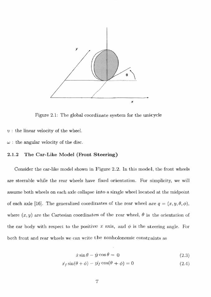
Figure 2.1: The global coordinate system for the uni ycle

V : the linear velocity of the wheel.

w : the angular velocity of the disc.

2.1.2 The Car-Like Model (Front Steering)

Consider the car-lik mod I shown in Figur 2.2. In this mod 1, th front wh els

are steerable while the rear wheel have fix d ori ntation. For simplicity, we will

assume both wheels on each axle collapse into a singl wh 110 at d at th midpoint

of each axle [16]. Th gelleraJized coordinates of the rear wh 1 are q = (x, y, (), ¢),

where (x, y) are the Carte ian coordinat s of th r ar wheel, e is the orientation of

the car body with respect to the po itiv x axis, and ¢ is the teering angle. For

both front and rear wheels we can write the nonholonomic con traint as

i; sin () - if cos () = 0 (2.3)

if sin(() + ¢) - VI cos(() + ¢) = 0 (2.4)

7

/--::-""7"""""---"-;:-""'---;::~~------------

y

x Figure 2.2: The global coordinate system for the car (front steering).

where (xf' Yf) is location of the midpoint of front axle that is given by

xf=x+lc:o e (2.5)

y! = Y + lsine (2.6)

where I is the distance betwe n th two axles. T king th d rivativ of quation

(2.5) and (2.6) gives the velocity as

:if = ± - l(} in e (2.7)

III = iJ + IB cos 0 (2. )

Solving equations (2.4), (2.7), and (2.8) to find iJ

iJ = tan ¢ Vl (2.9)I

ow the complete kinematic model i given as

Y I

~ sine 00Xl! cose 1 l 1 (2.10): = ,a , v, + ~ v,6

where Vl and V2 are the driving and t ering velocity inputs, re pectively.

8

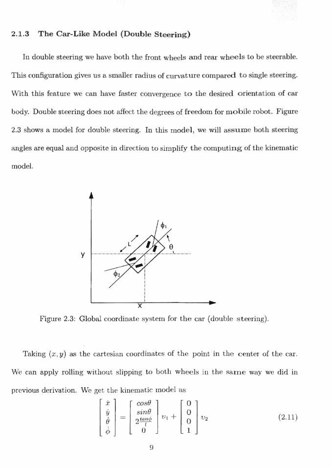
2.1.3 The Car-Like Model (Double Steering)

In double steering we hay both th front wh I and r ar wh 1 to b t rabl.

This configuration giv u a mall r radius of urvatur ompar d 0 ingl t ring.

With this feature we can hav fast r cony rg nc the d ir d ri ntation of ar

body. Double steering does not affe t th degr e of f[" darn for rno il robot. Figur

2.3 shows a model for double steering. In thi mod 1, we will urn both t ring

angles are equal and opposite in direction to simplify th computing of the kin matic

model.

y

Figure 2.3: Global coordinate system for th car (doubl st ering).

Taking (x, y) as the cartesian coordinates of the point in th nt r of th ar.

We can apply rolling without slipping to both wh I ill th same way w did in

previous derivation. W model as

(2.11)

9

where VI and V2 ar th driving and t ring v 10 it input r p tivel.

2.2 Curvature and Steering Angle (Double Steering)

To get a better under tanding of how th robot b h:ll for th ommand d

steering angle, we find the relationship betw n the t ring angl (double t ring

model) and the curvature. Thi relation hip i affine. If both r ar and front wh els

are fixed at a certain angle, the car will describ a cir ular path of certain radiu .

The curvature e(s) is equal to 1/R, wh Ie R i th radius of d scribed eirel . We

will describe how to find the radius experimentally and theoretically.

2.2.1 Finding Curvature from Simulation

We used equation (2.11) to find curvature by simulating the car motion at different

fixed steering angles. As expected, we got different circular paths, each with a

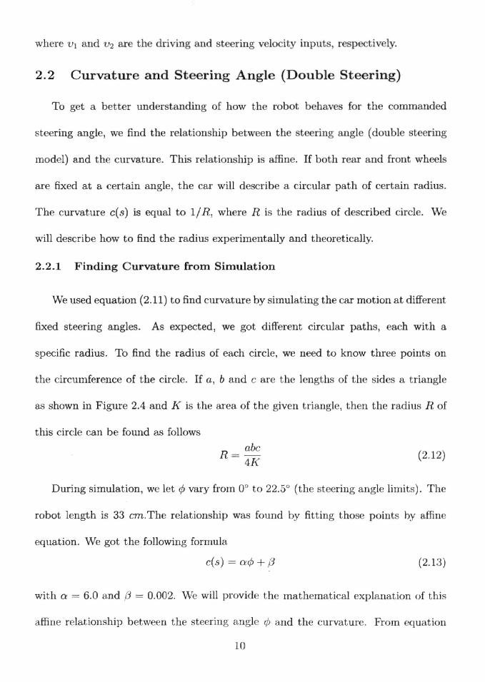
specific radius. To find the radius of each circle, we need to know three points on

the circumference of the circle. If a, band e ar th I ngths of th sid a triangl

as shown in Figure 2.4 and K is the area of th giv n triangl , th n th radius R of

this cirele can be found as follows

R= abc (2.12)4K

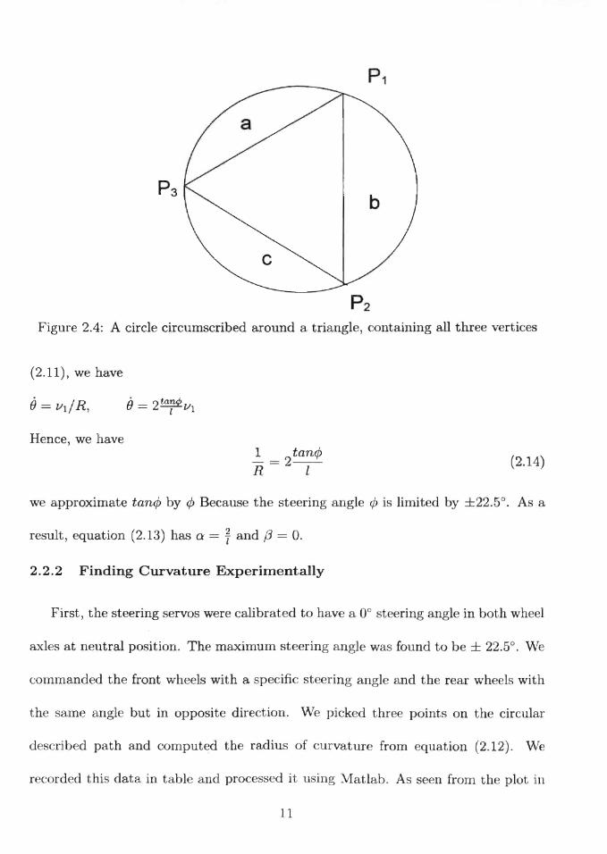
During simulation, we let ¢ vary from 0° to 22.5° (the steering angle limits). The

robot length is 33 em.The relation hip was found by fitting those points hy affin

equation. We got th following formula

c(s) = a¢ + 13 (2.13)

with Q = 6.0 and (3 = 0.002. We will provid th mathematical explanation of thi

affine relationship between th steering angle ¢ and the curvature. From quation

10

a

b

c

Figure 2.4: A circle circumscribed around a triangl , containing all three vertice

(2.11), we have

Hence, we have

~ = R

2tan¢ l

(2.14)

we approximate tan¢ by ¢ Becau th steering angl ¢ i limit d by ±22.5°. A

result, equation (2.13) has a = f and j3 = O.

2.2.2 Finding Curvature Experimentally

First, the steering servos were calibrated to have a 0° t ring angle in b th wh el

axles at neutral position. The maximum st ring angl was found to be ± 22.5°. W

commanded the front wheels with a specific steering ang! and th rear wheels with

the same angle but in opposite direction. We pick d three point on the circular

described path and computed the radiu of curvatur from equation (2.12). We

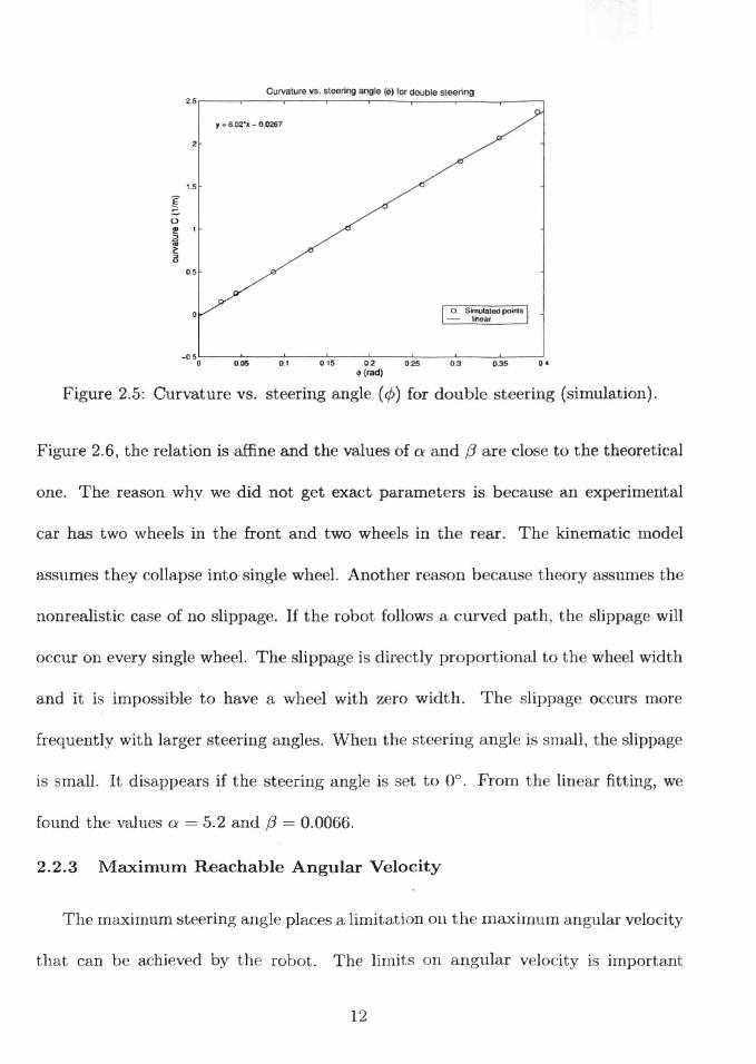
r corded thi data in tabl and pro es d it using Mat!ab. As seen from the plot in

11

Curvature VS. sleering angle ( ) for double sleenng 2.5r----.----r---.-----,---.----.---~.__-...,

y • a 02'~ - 0.0287

2

1.5

0.5

I 0 Smulatod po;,u I - Ii"....

-0 50~-~0.05:::---7'0.':-----:O~.'5=-----:O~.2----::-0.:-::25----:'0.3'=----'O.3:-::5----:'O' ~(rad)

Figure 2.5: Curvature vs. steering angle (</» for double steering (simulation).

Figure 2.6, the relation is affine and the values of a: and {3 ar do e to the theoretical

one. The reason why we did not get exact parameters is becau e an experim ntal

car has two wheels in the front and two wheels in the rear. The kinematic model

assumes they collapse into single wheel. Another r on b au e th ory urn th

nonrealistic case of no slippage. If the robot follows a urv d path, th lippage will

occur on every single wheel. The slippage is dire tly pr portional to th wh I width

and it is impossible to have a whe I with z ro width. Th lippag 0 illS mor

frequently with larger steering angles. When the ste ring angl i small, th slippage

is small. It disappears if the steering angle is set to 00 From th lin ar fitting, w •

found the values a: = 5.2 and f3 = 0.0066.

2.2.3 Maximum Reachable Angular Velocity

The maximum st ering angle places a limitation all th maximum angular velocity

that can b achieved by the robot. The limits on angular v locity i important

12

Curvature vs. steering angle C.) lor double sleering 2.5,-----,-----..--.,....---r---,-----.-----,.-----,

r. 5.3', - 0.076

o 2

1.5

°

05

o

0 Reoordod points II- linoar -0.5~-_=_=_--:':~---:~---:!=:-----=-=_-=~=~~=='_:l o 0.05 0.1 0.15 0.2 0.25 0.3 0.35 0.'

Q(rad)

Figure 2.6: Curvature vs. steering angle (¢) for double st ering (experimentally).

because control effort will be limited in real applications. The minimum radius of

curvature occurs at maximum steering angle which is in our case ±22.5°.

1 Rmin ~ --- (2.15)

ex¢max

The parameter ex is found experimentally to be ex = 5.2, th r for, R'l'nin ~ 0.5 m.

The angular velocity is constrained by

-Wmax ::; W ::; W max (2.1 )

where wand -w refer to counter clock wise and clock wi rotation, re p tiv ly. The

maximum angular velocity W max for a giv n constant linear pe d v can b comput d

from the following equation V

Wmax = D . (2.17) ~ "rntn

ther fore equation (2.16) becomes v v --- < W < -- (2.18)

Rmin - - Rmin

From th above equation, we can find the limits by substituting in th minimum

radiu of curvatur . The r lationship i plotted in Figure 2.7.

13

Reacha.ble Angular velocity

non-reachable (l)

non-reachable II)

-6 '--_L-----'--__--'-__--'- "'--__--'---"-_---J -15 -10 -s 0 10 1S

Linear velocity v (mls)

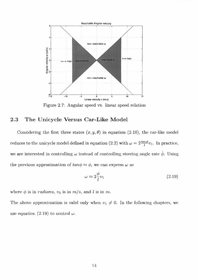
Figure 2.7: Angular speed vs. linear speed relation

2.3 The Unicycle Versus Car-Like Model

Considering the first three states (x,y,()) in equation (2.10), the car-like model

reduces to the unicycle model defined in equation (2.2) with w = 2 ta~cf>vl' In practice,

we are interested in controlling w in 't ad of controlling te ring angl rat ;p. U ing

the previous approximation of tan¢ ~ ¢, we can xpr w

(2.19)

where ¢ is in radians, Vl is in mj5, and l is in m.

The above approximation is valid only wh n Vl =!= O. In the following chapt rs, w

use equation (2.19) to control w.

14

Chapter 3 Hardware Description

In this chapt r the car h rdwar nd n or will be d tail d.

3.1 The Experimental Testbed

The MARHES Laboratory X-tr m robot (see Figure 3.1) ar b ed upon TXT­

1, a commercially available radio control truck from Tamiya Inc., with ignificant

modifications. The TXT-1 is de igned imilar to a full ize monst I' truck with an

aluminum ladder frame and multi-link su pension. Solid axle with a cantilev r

system allows for massive suspension articulation. The kit includes the hardware

and a second servo for four wheel teering. The servo (or servo ) are located n xt

to the axle for direct steering. The kit can operate on a 7.2 V or 8.4 V battery. We

used a 7.2 V battery to limit the speed. The robot has a servo controller for st ering

and a PWM speed controll r for forward/backward moti n.

An on-board notebook omputer provides the computational pow r for signal/im­

age processing, motion control and IEEE 802.11 b wir 1 ss n tworking. Als, PCM­

CIA Multi-function I/O card from National Instrum nts was u d for int rfa ing th

computer with a 'uite of analog and digital s n ors. Th uite of s nsor includ sIR

distance sensors odometer, CPS receiver, compass and st reo vision cam ra as w

will detail them in this chapter.

The included 3 Step mechanical sp ed controller is replac d by a ovak Super

Roost r reversible electronic speed controller. The new sp ed controller i u ed to

limit the current drawn by th driv motor, provide a safe transition from forward

15

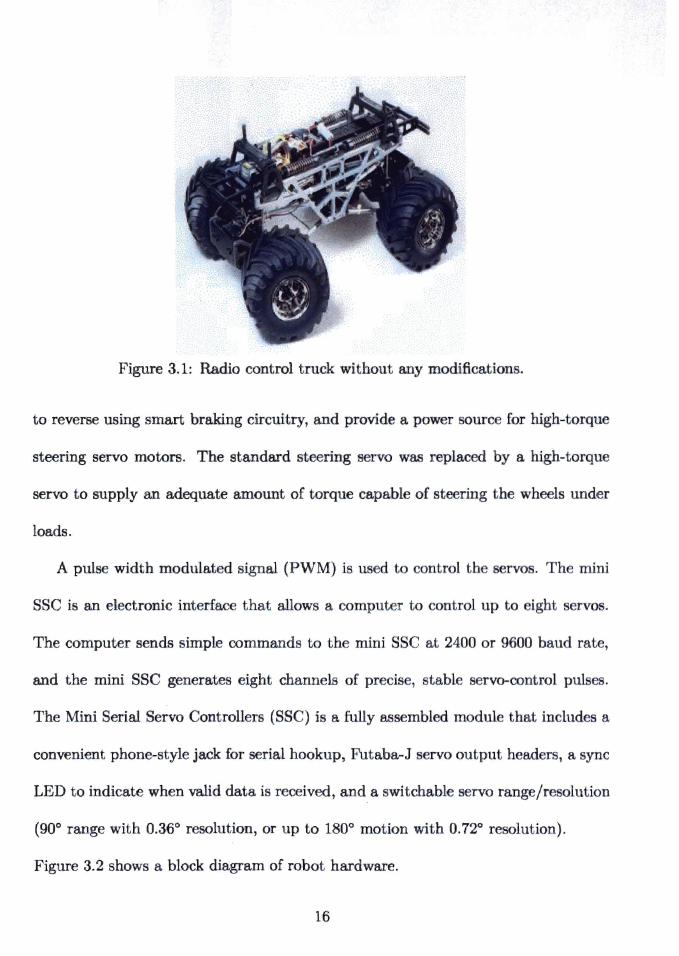
Figure 3.1: Radio control truck without any modifications.

to reverse using smart braking circuitry, and provide a power source for high-torque

steering servo motors. The standard steering servo was replaced by a high-torque

servo to supply an adequate amount of torque capable of steering the wheels under

loads.

A pulse width modulated signal (PWM) is u d to control th rvos. Th mini

SSC is an electronic interface that allows a comput r to control up to ight rvo.

The computer sends simple commands to the mini SS at 2400 or 9600 baud rate,

and the mini SSC generates eight channels of precise, table servo-control puls .

The Mini Serial Servo Controllers (SSC) i a fully ass mbled modul that includes a

convenient phone-style jack for serial hookup, Futaba-J servo output headers, a ync

LED to indicate when valid data is received, and a switchable servo range/resolution

(900 range with 0.360 resolution, or up to 1800 motion with 0.720 re olution).

Figure 3.2 shows a block diagram of robot hardware.

16

GnBoat:LNotebook

NIDAQ Card

Figure 3.2: Block diagram of robot hardware

The final shape of the robot after impl m nting all hardawr modifi ation i

shown in Figure 3.3. In the following s ctions we will d cribe th op ration of ach

h(\,rdware campon "nt.

3.2 Short Distance Sensors

This ensor was chosen because of the low price and simplicity of conne ting to

the multi-function I/O card. This sensor takes a continuous di tan e r ading and

reports the distance as an analog voltag with a distan e range of 20 em (~8 inch)

to 150 em (~ 60 inch). The interface is 3-wire with power, ground and the output

voltag .

17

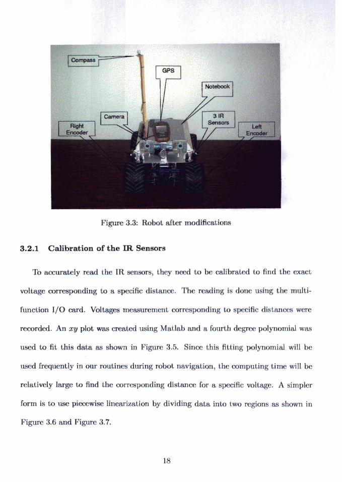
ICompass P==­

1< igure 3.3: Robot aft r modifi ation

3.2.1 Calibration of the m Sensors

To accurat ly read Lh lIt nsor, th y n d to b alibrat d t find th . act

voltag corr ponding to a p cHic distan . Th r ading is don usin r th muJti­

function I/O card. Voltag m asur m nt orr sponding to sp cifi di tane w r

recorded. An xy plot was cr ated u iog MaLlab and a fourth d gr polynomial was

used to fit this data as sbown in 1. igur 3.5. Since this fiLLing polynomial will b

used frequently in our routines during robot navigation, th computing tim will b

relatively large to find the corr ponding disLanc ror a sp cific voltage. A simpl r

form is to u e pieeewi e lineariza ion by dividing data into two r gions as shown in

Figure 3.6 and Figur 3.7.

18

Figure 3.4: Three Sharp GP2YOA02YK Infrar d rang r onfigur d in on unit.

3.3� Data Acquisition System

In order to interface data from the sensors with tb notebook, w us d tb 1

DAQCard-6024E for PCMCIA from ationa] Instrument. This i consid r d low­

co t compared to otber [card. Th analog output of hort di 1.. n

connected to the analog input of th ard. l'h output' r quadra ur

conn ct d to the inputs of the count 'r of th ac usation card. 1]- hni al p ifi a­

tions of tbi digital data acqui iLion card ar Ii t d in Tabl 3.1.

Table 3.1: I DAQ card-6024" pe ification

Analog Input Analog Output counters Digital. I/O

The I/O Connector Board

19

The voltage variation (11011) VS. dislance(m) for IR sensor 120r------.:..:.;......::...::..:.:..-....:.--,.--:--:...-~..:..:.:..,.::.:..:-.:.----r---_,

100

'0 III

80 I:IQ Y• 8.6'.' _ 74'" + 2.3e+002',? _ 3.4e+002'. + 2.3e.002

'b

o

o

'0 ()

o o

20

~.L5----'-----:',::-5-----:----;;;2.5:----~3

vollage(voll)

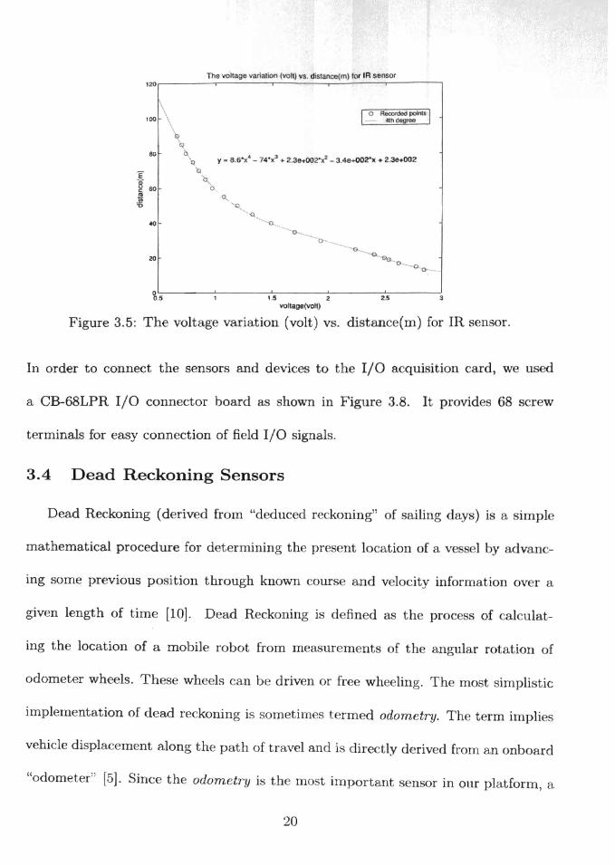
Figure 3.5: The voltage variation (volt) v distance(m) for IR sen or.

In order to connect the sensors and devices to the I/O acquisition card, w u d

a CB-68LPR I/O connector board as shown in Figure 3.8. It provides 68 screw

terminals for easy connection of field I/O signals.

3.4 Dead Reckoning Sensors

Dead Reckoning (d riv d from "d duc d re koning" of ailing d y ) i a impl

mathematical procedure for determining th pr sent 10 ation of a v 1 by advan ­

ing some previous position through known our and v 10 it inf rmation ov r a

giv n length of time [10]. Dead R ckoning is d fin d as th pr c of 1 ulat­

ing the location of a mobile robot fr m measurem nt of th angular rotation of

odometer wheels. The wh Is can be driv n or fr wheeling. h mo t impli tic

implementation of d ad reckoning i sometim t rm d odometry. Th t rm impli

vehicle displacement along the path of travel and i dire tly derived from an onboard

"odometer" [5]. Since the odom try j the rna t important n or in our platform, a

20�

The voltage varia 'on (voU) vs. dislance(m) lor fR sensor, reglon(1) 551----,~----,~---y-----.,.----y---r---r;:::;:::;:E=~~1

I 0 R8Ollf'ded paintl I ,- Unear

50 o

40 o

o

o

20

15

10

5,'------:"2':---:'1.-:-.--:-'1.6-;:------:"1.8-;:--~2---:':2.2:---2::'c.•:---,2:':.6--,2:':'.8-~3 vollage(voll)

Figure 3.6: The voltage variation (volt) vs. distance(m) for IR sensor, region(l).

clear understanding of of how it works is necessary. Angular rotation of the wheel

is measured by a rotary optical encoders attached to the wheel shaft. In the next

section we will describe the operation of the optical encoder.

3.4.1 Optical Encoder

An optical encoder con ist of a rotating disk, a light ourc , and a photod t tor

(light sensor). The disk, which is mounted on th rotating shaft, has od d patterns

of opaque and transparent sectors. As the disk rotates, th patt rus interrupt th

light emitted onto the photodetector) g nerating a digital or pul signal output.

The encoding disk is made from: glass, for high-resolution applications (11 to 16

bits), plastic (mylar) or metal, for applications r quiring more rugg d construction

(resolution of 8 to 10 bits). Quadrature ncoders can be used to determin dir ction

of rotation. This is done by adding a second channel, off t from th first, by 90°. A

po sible tup is shown in Figure 3.9. Channel A can be used to provide the number

21�

The vollage variation (volt) vs. dlslance(m) IOf IR sensor reglon(2) 90

I~ ~PO·lI·1 85 0

80 0

75 0

y • - 86"' + 1.4e+002 :§>o 0 Ql g ~ '" 65 0 "0

60 0

055

50

45 065 0.7 0.75 0.8 0.85 0.9 0.95 1.05 1.1 1.15

vollage(volt)

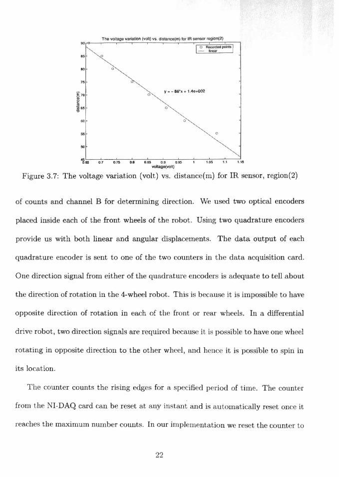
Figure 3.7: The voltage variation (volt) vs. distance(m) for IR ensor, region(2)

of counts and channel B for determining direction. We used two optical encoders

placed inside each of the front wheels of the robot. Using two quadrature encoders

provide us with both linear and angular displacements. The data output of each

quadrature encoder is sent to one of the two count r' in th data cqui ition ard.

One direction signal from either of th quadratur n oders i ad quat to t 1L bout

the direction of rotation in the 4-wheel robot. Thi is b au e it i impo ibl to h v

opposite direction of rotation in each of the front or r ar wh I. In a difF r ntial

drive robot, two direction signals are requir d b caus it i po ible to hav on whe I

rotating in opposite direction to the other wh 1, and hence it is po sible to spin in

its location.

The counter counts the rising edges for a sp cified period of time. The count r

from the NI-DAQ card can be reset at any in tant and i' automatically r set on e it

reaches the maximum number count. In our impl mentation we reset the count r to

22�

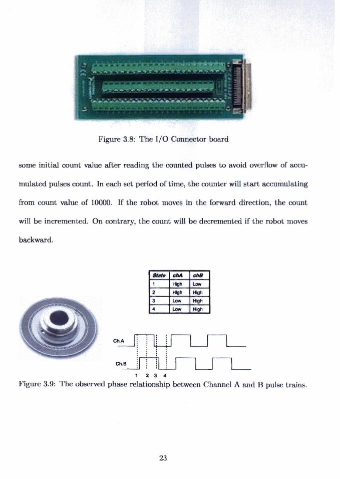
Figur 3.8: The I/O onn ct.or board

orne initial count value aft r r ading th count d p to avoid v rHow of accu­

mulated pulses count. In each s t period of tim, th counter will tart accumula(,ing

from count value of 10000. If the robot move in th forward dir ction th ount

will be incremented. On contrary, tb count will be d cpm nt d if tb robot move

backward.

StMlI eM ebB

1 High Low

2 HIgh High

3 Low High

4 Low High

1 2 3 4

Figure 3.9: The ob rved phase r lation hip betw n bann 1A and B pul train.

23�

3.4.2 Installing Optical Encoder for the Car

We have used optical encoder from Agil nt 'D elm l.ogi s. Th odom r

consists of the HEDR-8000/8100 S ri s ncod r. It u s r fI. tiv t hnology to

sense rotary or linear position. This sen or con i ts of an LED light our and a

photodetector IC in a single SO-8 surface mount packag . W hav 1.1 d r fl ctive

codewheel HEDR-5120-H-12. The numb r of puis for one ompl te r volution i

408. The surface mount chip is mostly affect d by ambi nt lights, therefore, th best

place to install it is inside the wheel. Doing 0 will al 0 give the odometry system

protection against any damages from crashing.

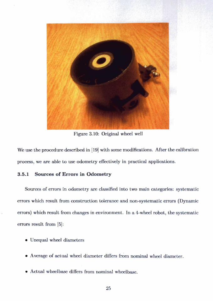
For installing the code wheel on the shaft, we first have to provide enough pace

inside the unmodified upright part. This is done by milling a distance equal to the

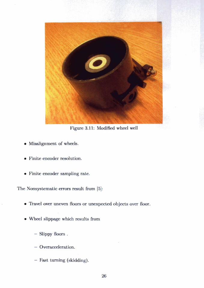
width of the codewheel. Figure 3.10 and Figure 3.11 how the wheel well before and

after modifications. The codewheel is mounted on th h ft of th ar wh I in the

milled space as shown in Figure 3.12. From th data h t, it an b s n that the

spacing between the code wheel and the chip is v ry important and should b done

as specified (2.03 ± 0.51mm) to get good results. The 1 troni cir uit board of the

chip is placed inside the end of the upright, ke ping r comm nd d spacing distan

with codewheel.

3-.5� Calibrating the Mobile Robot

Since the odometry syst m will depend on s~me parameters of the robot, the

robot must be calibrated. Calibrating odometry for a 4-wh el robot is bas d on

accurate measurement of the orientation angle as w 11 as translations and rotations.

24�

We use the procedure de cribed in [19] with orne modifications. Aft r th alibration

pro w., ar abl to u' adorn try fli LiV1 ly in pr eLi aI appli ati n1

3.5.1 Sources of Errors in Odometry

Sources of errors in adam tryar clas ifi dint two main yet maLic

error which r uit from construction tol ran and non-s t mati fror (Dynamic

error) which r ult from chang- in environm nl. 1n a 4.-wh I robot, th yst matic

error re ult from [5]:

• Unequal wheel diameters

• Average of actual wheel diam ter differs fr~m nominal wheel diam t r.

• Actual wh lbase differs from nominal whe Ibase.

25�

• Mi� alignment of wheel .

• Finit� lution.

• hnit ncod r sampling rat.

The on y t, matic error r suit [rom [51:

• Tra'" l OVi r un '" n floor or unexp t d obj OV r fI r.

•� Wh I lippage wbich r ult [rom�

- tippy floors.�

- Ov race leraLioIl.�

-� as turning ( kidding).�

26�

Figur 3.12: InstaLLed codcwh ei and phoL d t or

- External forces (interaction with xt mal bodi ).�

- Internal forces (castor wh is).�

- lon-point whe 1contact with th floor.�

The calibration proc i don to minimiz syst mali ITor.

3.5.2 Odometry Equations and Calibration Param t rs

Wh n th wheels of the robot roU n tb ground, th numb r of pul g n rat d

from rotary encoder inside each front wh "i i proporLi nal to th tra\!' U d dis tan .

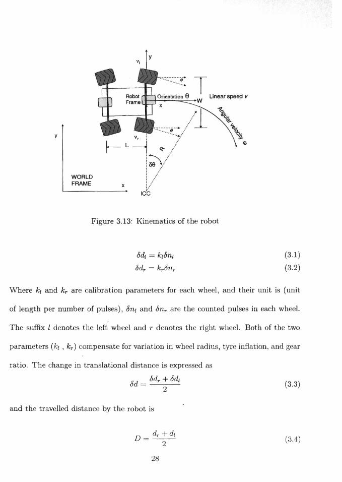
The kinematic modeling of the robot requir [ram. Figur 3.13 how

the robot and its reference fram (x, y, 0) Locat midway b Lw n h fr nt wb t.

In our robot, two encod rs are installed insid ach front wb I.

The equation, which r tat s the change in travelled d' tance with the hang of

number of puts in each wh el, is

27

y

WORLD FRAME

Figure 3.13: Kinematics of the robot

od[ = k[on[ (3.1)

8dr = kronr (3.2)

Where k[ and kr are calibration paramet r for each wheel, nd th ir unit i (unit

of length per number of pulses), on[ and onr are th ount d pulse' in each wh 1.

The suffix l denotes the left wheel and r denot th right whe 1. Both of the two

parameters (k[ , kr ) compensate for variation in wh el radiu , tyre inflation, and g ar

ratio. The change in translational di tance i expressed as

(3.3)

and the travelled distance by th robot i

(3.4)

2

where d.r and dl ar evaluat d at a h tim p

(3.5)

(3.6)

The orientation angle of the robot 8 after trav lling a di tanc D i xpr d in

terms of each wheel travelled distance as

8 = dr - dl (3.7)W

and the rotational displacement is computed in the same manner as

08 = ocl.,. - odl (3.8)W

where W is the robot base width.

The effective width in this case is the distance between the two encoders. By deriving

equations (3.3) and (3.4), we can decompo e the robot motion into translation

component and a rotation component. Th lin ar v 10 ity v and an r v 1 ity w

of equation (2.1) are now expressed as

V r +VI V=--- (3.9)

2

V r - VI W= (3.10)HI

3.5.3 Calibration Procedure

First, the robot's front and rear wheels must be aligned at 0° st ring angl . This

is done using a traight edge that touches both sid tire. To calibrat both k1 and

kr parameters, we run the robot in a straight path for short distanc (5 m ter ) and

29

measure the tra lled di tanc u ing m uring tap . B knowing numb r of pul s

accumulated during this travelled di tan ,w f th two

parameters. The final paramet r to calibrate i th width, whi h is done by

running the robot one complete eirel that nd at th am initi 1 t rting point. W

initialize the robot heading angle to be 0° in Cart sian oordinat . Th r ultant

orientation angle after returning to the starting point of th ir ular path will be

21r after one complete circle. By knowing both of the a cumulat d pul es from the

front wheels, we can calculate the base width from equation (3.). ow we an do

fine tuning for the three parameters kl , kr and W by commanding the robot to

move for larger distance (20 m or more) in straight and circular paths many times.

We use the kinematic model to update (x, y, 0) based on odometric displacements.

Each time we tune the three parameters to match real position until we get the best

position results. In the case of straight line path the final heading angle should be

zero as we start from zero head angle. So w modify both kl and kr to g t 0° head

angle. Table 3.2 show the final valu s of calibration param t r .

Table 3.2: Calibration param t rs

Parameter Value k l 0.1178 em/pulse count kr 0.1184 em/pulse count W 22.9 em

30

3.6 Vision Cams Unit

The vi ion ensors are important for navigation and ob ta 1 avoi In. W us d

two cameras mounted on the front of the v hid facing forward. Tb the robot

its exact position at all time, allowing it to sen tb 10 ation of obj t and to tra k

a predefine color. In our work, we use a simple color d t tion b d on a t reo

vision system to compute the distance from the robot to a targ t. Tb

of the cameras used are shown in Table 3.3.

Table 3.3: Camera specifications

I Interface IEEE-1394a (FireWire) 400 Mbps, 2 ports (6 pins) Camera Type IIDC-1394 Digital Camera, Vl.04 Specification compliant Sensor Type . Sony Wfine* 1/4" CCD Color, progressive, square pixels Resolution VGA 640 x 480 I

Optics Built-in f 4.65 mm lens, anti-reflective coating Power Supply 8 to 30 VDC, by 1394 bus or external jack input

Consumption 1W max, 0.9 W typical, 0.4 W sleep mode Dimensions (W x H x D) 62 x 62 x 35 mm

3.7 Compass Sensor

Electronic compass is an essential component of the olution to n of the long-

standing robotics problems Where am I? The compas is n d d b cau e it an

compensate for the foremost weakness of odometry. In an odometry b d position­

ing method, any mall momentary orientation error will cau e a con tantly growing

lateral positioning error [5]. The advantage of u ing a compas rath r than a gyro

is that a compass gives the heading angle directly. The gyro require integrating

the angular velocity to get the heading angle. The compas will provide th hading

31

angle me urement updat in th K lman filt r w will xplain lat r. d id d

to use th 1655 analog comp n or from Din mor In trum nt ompan. Thi

sensor provides a ratiom tri output on two hann I Th outpu wing from ap­

proximately 3.2 V to 1.8 V in a in jcosin f hion. It will r turn t th indi at d

direction from a 90° displacement in approximat ly 2.5 conds with no ov r wing.

Technical Specifications of 1655 analog comp sen or ar list d in Tabl 3.4.

Table 3.4: Specifications of 1655 analog ompass sensor from Din mol' Sen or

Power 5-volts DC @ 19 rnA. Since rise time is only 90 nanosecond , input current may be pulsed to save power.

Outputs Dual analog channels, 2.5 V ± 0.75 V swing (total voltage swing rail to rail, approximately 1.50 V), 4 rnA DC signal. May feed direct to A-D front end of microprocessor.

Weight 2.25 grams Size 12.7 mm diameter, 16 mm tall Pins 3 pins on 2 sides on .050 centers Temp -40 to +85 degrees C

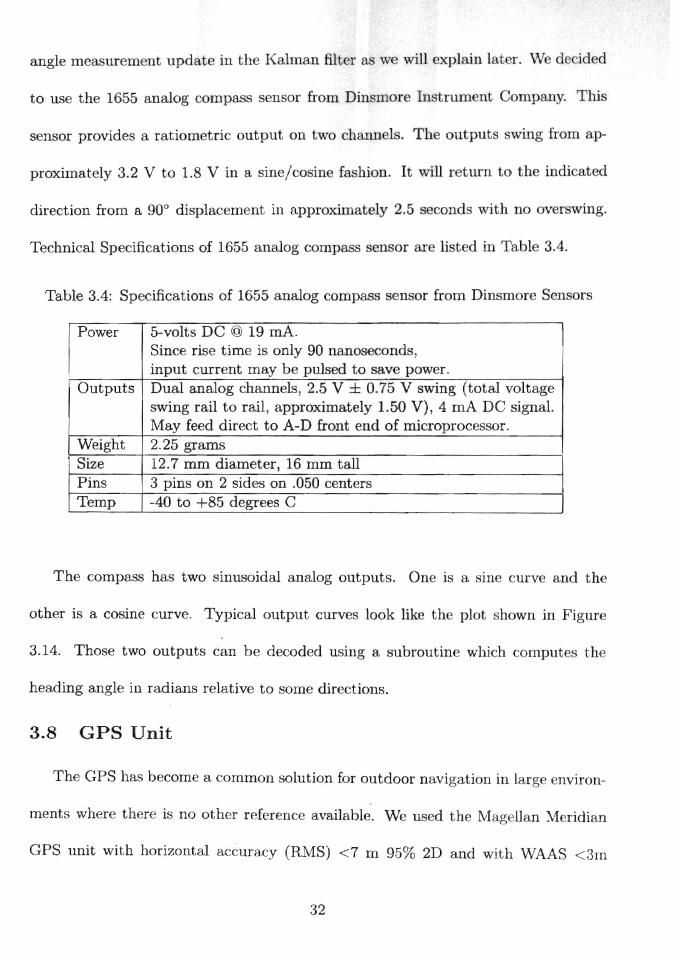
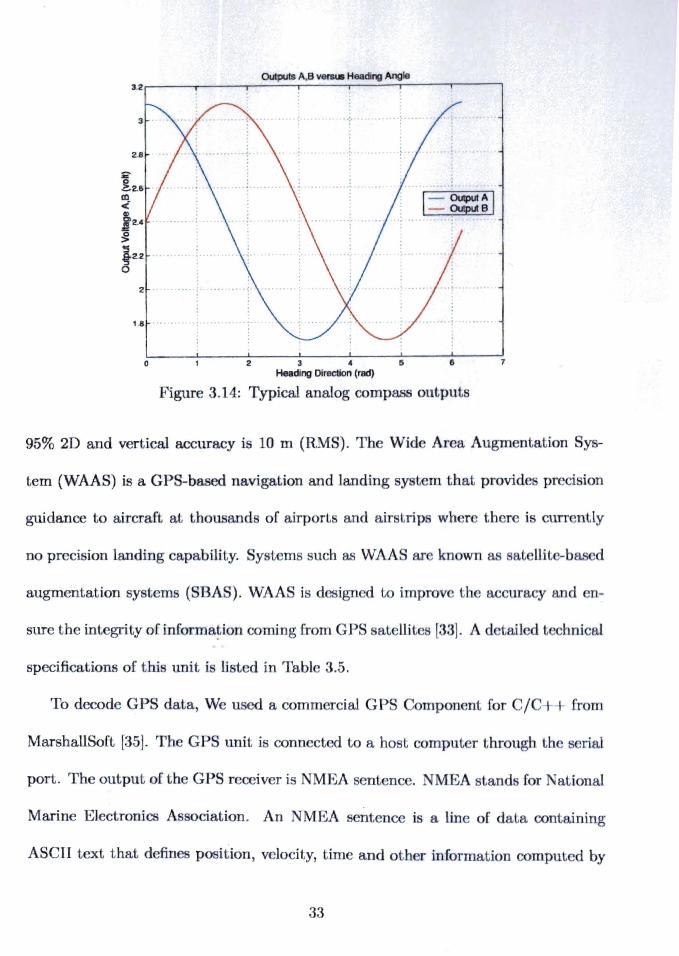
The compass has two inusoidal analog outputs. On i a in urv and the

other is a cosine curve. Typical output curve look lik th pI t shown in Figur

3.14. Those two outputs can be decod d using a subroutin whi h comput the

heading angle in radians relativ to orne dir ctions.

3.8 GPS Unit

The GPS has become a common solution for outdoor navigation ill larg nVlron­

ments where there is no other reference available. We used the Mag Han M rid ian

GPS unit with horizontal accura y (RMS) <7 m 95% 2D and with WAAS <3m

32

Outpuis A,B v 1S1.8 Heading Angle3.2.-----.----.-....:.--,-----.--.=.-,---,..--------,

2.8

2" o ~2.6 lD <{

&1l! 2.4

~ '5 ~2.2

o 2

1,8

o 2 3 4 !5 6 7

Heading Direction (rad)

Figure 3.14: Typical analog compas outputs

95% 2D and vertical accuracy is 10 m (RMS). Tb Wid Ar a Augm ntation S ­

tern (WAAS) is a GPS-ba ed navigation and landing y t In \'hat provide pr ci ion

guidance to aircraft at, Lhou and of airp rL and air Lrip

no pr ci ion Landin capability. Sy L much as WAA 1m wn d

augm ntation y t m ( BA ). WAA i d ign d \'0 impr Vi Lh aura yan n­

ure the integri ty of infarma~ioncami og from P at II it [331. A d tail d I, hn i aL

sp cifications of thi unit i ti ted in Tabl 3.5,

To decode CPS data, We us d a camm rcial GP amp n nt [or I + 1- from

Mar haUSoR (35}. Th GE S unit is connected La a bo Lcomput r through h rial

port. The output of the GPS river is MEA ent nee. M· A Land [; rational

Marin ELectronics A 0 iaLion. An MEA ent n a lin of data containing

ASCII text that d fin po i ion, Vi Iocity, time and oth r information comput d by

33

Table 3.5: CPS t chnical sp cification

Position Update Rate (per second) 1 Time to First Fix: Cold <2 Time to First Fix: Warm <1i

Time to First Fix: Hot (seconds) 15 Maximum Velocity (mph) 951 Maximum Velocity (km/h) 1530 Weight (gm) 227

. Display Size Height (inches) 2.2 Display Size Height (mm) 55.9 Display Size Width (inches) 1.75 Antenna Quadifiler Helix. Horizontal Accuracy (meters) <7 Horizontal Accuracy (RMS) 95 % 2D Horizontal Accuracy -RMS wi WAAS (meters) <3 Horizontal Accuracy (% RMS/WAAS) 95 % 2D Vertical Accuracy (meters RMS) 10 Velocity (knots RMS) 0.1 Battery Type AA Battery Quantity 2 Battery Life (hours) 14 Receiver WAAS Enabled Yes Waterproof (IEC-529 IPX7 Standard) Yes Operating Temp Min (C) -10 Operating Temp Max (C) 60

34

the GPS river. tting r ud with hi f d t no

parity, and no top bit. tandard provid a larg rang of nt n

but many relate to non-GPS devi and om oth r ar GPS r 1 t d but rar ly

used. Most GPS receivers al 0 have a binary mod but it i normall b t to I' rYe

the use of binary GPS proto ols for appli ation that rally r quir th ir u , u h

those requiring position updates of greater than once per and. In our work w will

be dealing with two cornman types of MEA sentence which are the GPGGA and

GPRMC. The GPGGA stands for Global Positioning Sy tern Fix Data. An exampi

of the structure of the GPGGA sentence is shown below:

$GPGGA, 123519,4807.038 ,N ,01131.000,E,l ,08,0.9,545.4,M,46.9,M" *47

An explanation of this MEA sentence is given in Table 3.6 [34]. The GPRMC

NMEA sentence gives position, velocity, time and course data. It stands for the

Recommended Minimum. An example of th structur of th GPRMC nt n

shown below :

$GPRMC,123519,A,4807.0~8,N,01131.000,E,022.4,084.4,230394,003.1,W*6A

An explanation of this GPRMC NMEA senten e is giv n in Tabl 3.7 [34].

3.9 Power System

An important problem to overcome was supplying different voltage 1 v Is to op­

erate the additional hardwar components. We' have solved this probl m with the

addition of a Battery Booster 12 circuit. This circuit eliminate the n ed for a 9 V

battery for the Mini SSC II serial servo controller b' ard from Scott Edwards Ele _

35

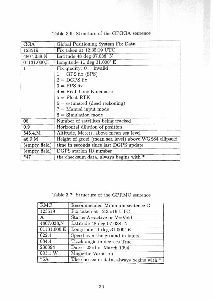
Table 3.6: Stru tur of th GPGGA nt n

GGA Global Positioning System Fix Data 123519 Fix tak n at 12:35:19 UTe 4807.038,N Latitude 48 deg 07.038' N 01131.000,E Longitude 11 deg 31.000' E 1 Fix quality: 0 = invalid

1 = GPS fix (SPS) 2 = DGPS fix 3 = PPS fix 4 = Real Time Kinematic 5 = Float RTK 6 = estimated (dead reckoning) 7 = Manual input mode 8 = Simulation mode

08 Number of satellites being tracked 0.9 Horizontal dilution of position 545.4,M Altitude, Meters, above mean sea level 46.9,M Height of geoid (mean sea level) above WGS84 ellipsoid (empty field) time in seconds since last DGPS update (empty field) DGPS station ID number *47 the checksum data, always begins with *

Table 3.7: Structure of the GPRMC nt n

RMC Recommended Minimum sentence C 123519 Fix taken at 12:35:19 UTC A Status A=active or V=Void. 4807.038,N Latitude 48 deg 07.038' N 01131.000,E Longitude 11 deg 31.000' E 022.4 Speed over the ground in knots 084.4 Track angle in degrees True 230394 Date - 23rd of March 1994 003.1,W Magnetic Variation . *6A The checksum data, always begins with *

36

tronies. The lR n or I' qUIr a 5 volt D uppl. u d th r gula d 5 v I

from the connector board of the a qui i ion ard that i uppli d b th not book

battery. The second problem w upplying nough pow I' to th v hi 1, inc it

carries more weight than it was d igned for and al 0 now h high torque rv

sensors, speed controller, etc., which are xtra load on th p w r t m. Th two

options to solve those probl m are adding additional batteri or r placing th x­

isting battery with a more powerful one. The problem with adding more batteries

is that there is no convenient place on the chassis to store th m. Also adding xtra

batteries will increase the load on the robot. Our po ible solution is to have a single

battery with large battery capacity (5000 mAh). Using a fully harged 7.2 V battery

with 3000 mAh capacity, the average runtime is about 30 minutes.

3.10 On Board Computer

The ouboard comput r along with th multifun tion a qui ition 'ard provid a

computational power for sensory data pro ssing. We d id d to us a S ny VAl

SRX77P notbook. Using su h a not book sav s th tim f building a PC on th

robot. The notebook is fast, lightweight, and has low pow r consumption. Th

processing unit used in other exp rimental testbeds vehicles ar bas d on a micro­

controller [20],[14], ihis might limit the capabilities of th robot. Using a notebook

will provide a large disc space for writing code, a fast processing speed, a standard

communication interfaces and a built in efficient battery. Two serial ports wer

needed to interface both the sse and GPS r iv r. An USB to serial port converter

from Keyspan was u ed Becau e th notebook doe not have a serial port. The

37

I e span USB 4- Port rial ad pt r aHo\) f ur rial d vi to b nn t d to

single USB port.

Table 3.8: otebook p cifi ati n

Processor Low Voltage Mobil Int I PentiumIII processor 800A MHz

L2 Cache Memory 512 KB (CPU Integrated) Hard Disk Drive 20 GB C/D Partition 40% and 60% (approximation) Standard RAM 128 MB SDRAM (Expandable to 256 MB)

(PClDO unbuffered DIMM memory modules) LCD Screen 10.4" XGA (1240 x 768) Wireless LAN ' Communication IEEE802.11 b

(IBSS Ad hoc mode support, DS-SS modulation) Max. 11 Mbps data transfer speed (approximation) Max. 100 meter communication di tance(approximation) 2.4 GHz band frequency Wireless channels 1 to 11 64, 128 bit Network key length

Power Source 16V DC/AC 100-240V Battery Lithium-ion Dimensions 10.2" (w) x 1.1" (h) x 7.7" (d)

(259 mm x 27.8 mm x 194 mm) Connection Capabilities 1 USB port Phon line (RJ-ll) p rt

Ethernet port LLINK (IEEE 1394) p rt, 4-pin S400 styIe

In the next chapter, we will discuss the oftware archite ture impl m nt d in this

thesis.

38

Chapter 4 Software Integration

This hapt r pr sent the oftwar d v 1 pm nt of our d ign d hi 1 .

4.1 Software Architecture

The current softwar ar hitecture i impl and fl. xibl for an futur updat.

The block diagram shown in Figure 4.1 give a d tail d stru tur of th on ral

architecture implemented on the ARHES TXT robot. It on i t of hardwar

dependent software, logical sensors and controllers. Thi architecture allow the ve­

hide to exhibit intelligent autonomous behavior. We used an object-ori nt d C++

decomposition to provide abstractions for the component of the y terns. Compo­

nents are implemented using classe .

4.2 Real-Time Issues

Our vehicle control r quir s 11 al-time p rforman finiti n

of real-time. The definition given in [31J is as follow "A real-time y tem i on in

which the correctness of the computation not only depend upon th logi al orr ct­

ness of the computation but also upon the time at which the r ult i produced. If

the timing constraints of the system are not met, ystem failure i said to have oc­

curred." A brief discu sion of real-time issue lik d termini m and jitter is giv n in

[18]. Real-time control applications p rform a d fin d task periodi ally. Th task is

performed b fore the new pro essor period tarts. Figure 4.2 how proc s or activ­

ity during running time. Th hard r aI-time performance i difficult to b achi v d

39

Logical Sensors Controllers

Obst. voidanc

,,,,,

. ,

~ ~ •• .. .. • ... __ ... _J

Figure 4.1: Control ar hitecture scheme.

using gene

Processor Activity

J_T~k m···l····~·············i .. T"k I..~ Lj T...

Time

Figur 4.2: Real-time control.

4.2.1 Windows Family Operating Systems

The operating sy tern u d was Micro oft Windows XP. Some of th re on for

this hoice include[36]

40

• Th incr asing pow 1: and d lining pri of Window XP pI tform .

• Th many appli ations allabl on th pIa £ rro.

• The vari ty of developm nt tools availabl on th platform.

• The richnes of the Mi ro oft win32 Application Pr grammin Int rf (API).

• The large number of d veloper , support p r onn I, and nd u r who r

familiar with the system.

The Windows XP is not inheren ly a real-time op rating sy t m.

method to improve its performance is by using real time extensions. Venturcom is

providing RTX extensions for real-time performance. RTX enabi Windows XP,

Windows 2000, or Windows NT to function as both a general-purpos op rating

system and a high-performance real-time operating [37J. In our operating system

we did not experience with th xt n ion , how v r, th y ould b olution t

improve the performance.

4.3 Multi-Threading and Timing Functions

In most PC operating sy tern' the central pro sing unit C.P.U i not abl to

run two piec s of code at exactly at th am tim. The op rating y t m olv s

this problem using time slicing. In time slicing, th microproce or tim har d

among piec of code called thread . Each thr ad i giv n a portion of th micropro­

ces or's time. Hence the thread thinks it h the whol mi ropro e or tim whil

it is actually shared among other thread . The d tail of how th operating ystem

implements multi-thr ading ar b yond th op of his the is.

41

gr at advantag of u ing window b d p ra ing m i h up rt

of multi-thr ading. ulti-thr ading i a wa to I t pI'ogr m do m r than n thing

at a time. It i implemented within a ingl pr gram running n a ingl m.

It involves an operating sy t m allowing pI' gram to pli t tw n multipl

thr ads of x cution. In our main program w n d im d fun tion alls

at exact sp cific rates. We need to run our dill r nt ind p nd ntl, h

at a specific rate to get good r suIts. On m thod to do this i t u int rrupts

but this method is not recommend d under Window XP. Th oth r m thod i

to use the multimedia library. This multimedia tim r provid s a high ac uracy of

timing schedule as we monitored the microproce or p rformanc. This ac uracy

is extremely lowered when using functions that are computationally intensive like

image processing routines. The multimedia timer u es a eparate hread to generate

timed function calls in the applicati n. Th handling of th thr ad is done internally

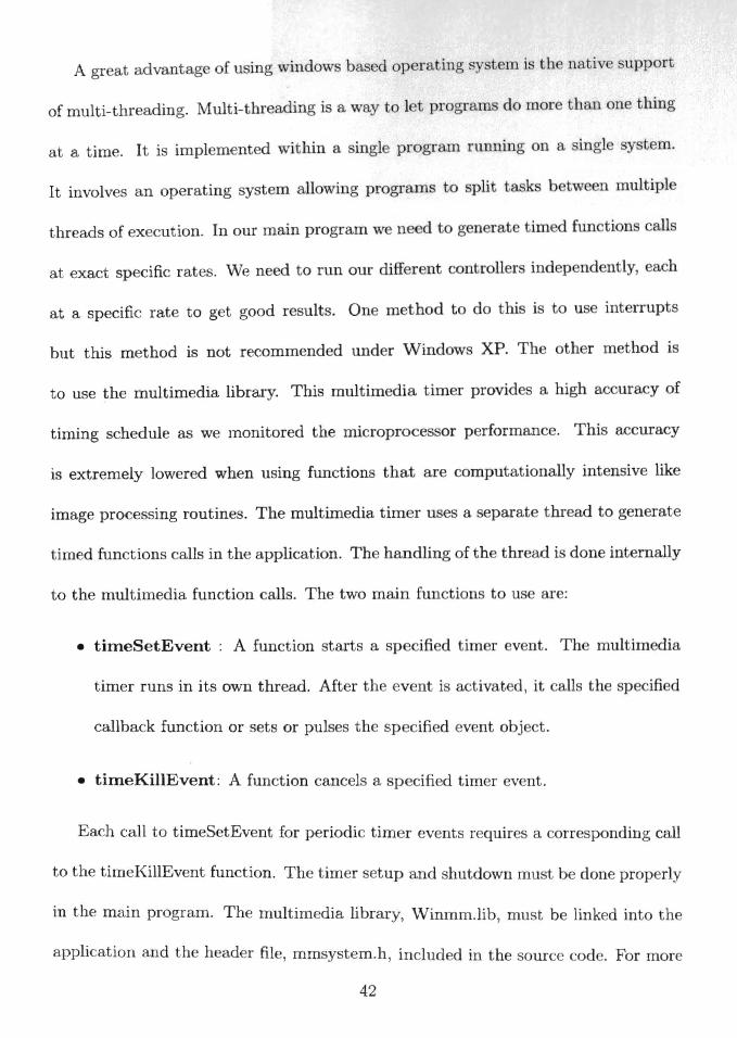
to the multimedia function alls. Th two main fun ti n t u ar:

• timeSetEvent : A function tarts a sp ifi d tim r v nt. Th multim di

tim r runs in its own thread. Aft r th v nt is tiv t d, it Us th

callback function or sets or pulses th sp ifi d ev nt obj t.

• timeKillEvent: A function cancel a p 'ifi d tim r ev nt.

Each call to timeSetEvent for periodi timer ev nts r quir s a orresponding call

to the timeKillEvent function. Th timer etup nd hutdown mu t b done properly

in the main program. Th multimedia library, Winmm.lib, mu t be link d into the

application and th h ad r file, mmsy tem.h includ d in the sour e code. For more

42

information about multirn dia library, th M D librar. ing multi-thr ading

enables us to switch b tw en behavior through g n r ting and t rmina ing tim d

events.

43

Chapter 5 Tools for Vehicle Control

This chapter d cribes the tool w implem nt d for our d ign d robot.

5.1 Velocity Controlled Robot

Working with a kinematic model only is impl and mak th r aliz tion of th

controller possible. The usual input for a 4 wheel mobile robot ar th t ering angle

¢ and speed. Dealing with these two input might in rease th difficulty of control­

ling the robot since many control laws are express d in t rms of linear and angular

velocity. One can think that a higher level controller (plann r) generate the de ired

velocities and a lower level controller deals with the car dynami (mass, inertia,

etc.). As a result, we need a transformation that transforms the input commands

of linear velocity (v) and angular velocity (w) to motor peed and steering angle ¢.

Most application for controlling mobile robots requir ur t mat hing b tw n

commanded velocity and the actual velocity. This prop rty n not b a hi v d using

an open loop controller. Hence there is a need for a do d loop ontroller to n ur

the convergence of the actual velocity to the command d v 10 ity. PID cantrall rs

have been used effectively for many years in indu try. i e [23] has a good di ussion

of adjusting the PID gain, K p , K i , and K d . Figure 5.1 show a blo k diagram of

the velocity controlled robot. The PID controller is design d to match the m asur d

velocity with commanded one.

44

Kinematically Controlled Robot

Actual Robot

VmeasuredVdesired

prD (OmeasuredController(Odesired

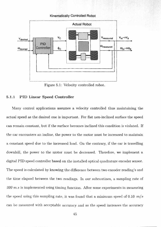
Figure 5.1: Velocity controlled robot.

5.1.1 PIn Linear Speed Controller

Many control applications assumes a velocity controlled thus maintaining the

actual speed as the desired one is important. For flat non-inclined surface the speed

can remain constant, but if the surface b comes inclined thi ondition i viol t d .. If

the car encounters an incline, th power to the motor mu t b in r as d to maint in

a constant speed due to the incr as d load. On th ontrary, if th ar i traY lling

downhill, the power to the motor must b d creased. Therefor, w· impl m nt a

digital PID speed controller based on the in tailed optical quadratur ncod r n or.

The speed is calculated by knowing the differ nce between two ncod r r ading' and

the time elapsed between the two I' adings. In our ubroutin , a ampling rate of

200 m. s is implemented using timing function. After om xp rim nts in m asuring

the speed using thi sampling rate, it was found that a minimum sp ed of 0.10 m/s

can be measured with acceptable accuracy and as the spe diner as the accuracy

45

improve. The robot lin r locit i a tuat d b two D m t r . pr ximat

the y tern as a fiT t ord r tern. A fir t ord r t m h th form

} (5.1)G(s) = 1 + 7S

where K is a constant and T is the tim can taut of th sy m r pan which is th

time it takes for the step r ponse to rise 63% of it final vall. Th tim onstant

depends upon the robot's environment. It was found xp rim ntaH to b around

1.5 seconds for even ground. A simple standard digital PID ontroller shown in

F}gure 5.2, has the general form:

(5.2)

R(s) +

Figure 5.2: A PID controll r

wh r u i the change in velocity, the variabl repr ent th tracking error

(the difference between the desired input value and· the actual output), kp i the

proportional gain, ki is the integral gain and kd is the derivative gain. The gain

46

parameters kp , ~ and kd re ho n 0 g th b m p rform 11 and

stability.

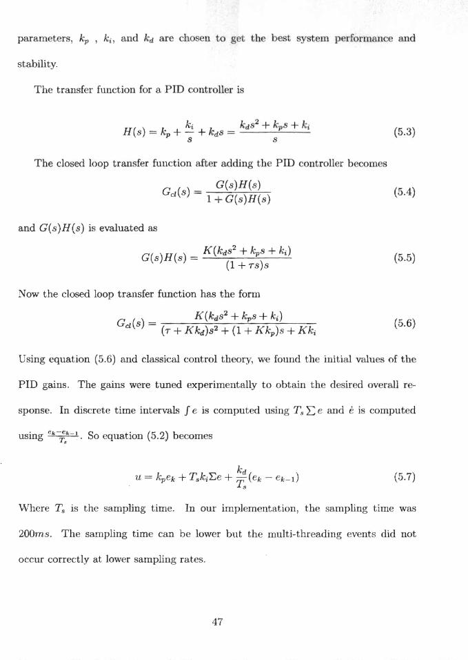
The transfer flmction for a PID controll r i

(5.3)

The closed loop transfer function after adding th PID ontroll r b om

G( )H(s) Gcl(s) = 1 + G(s)H(s) (5.4)

and G(s)H(s) is evaluated as

(5.5)

Now the closed loop transfer function has the form

Using equation (5.6) and classical control th ory, we found th initi I valu of th

PID gains. The gains were tuned xperim ntally to obtain th d sir d v rall r

sponse. In discrete time intervals Ie i computed uing Ts E and' i omputed

llsing ek-;.k-I. So equation (5.2) becomes

(5.7)

Where Ts is the sampling time. In our implementation, the sampling tim was

200ms. The sampling time can be lower but the multi-threading v nts did not

a 'cur correctly at lower sampling rates.

47

Smoothing Filter Using Holt Exponential Smooth r

This simpl and wid ly u d r cur ive £11 r is obt on d b it ring

Yt = aXt + (1 - a)Yt-1 (5. )

where a < 1 is a tunable smoothing pararn t r. Thi filt r can bud onlin to

smooth the output commands and sensor' measur ment . Thi allow u t 'rnootb

the output commands of digital PID spe d controller. This low-p filter giv s most

weight to most recent historical values and thus provides the b is for a nsible

forecasting procedure when applied to trend, seasonal, and irregular components

(Holt-Winters forecasting). The parameter a was tuned experim ntally to g t the

best possible performance.

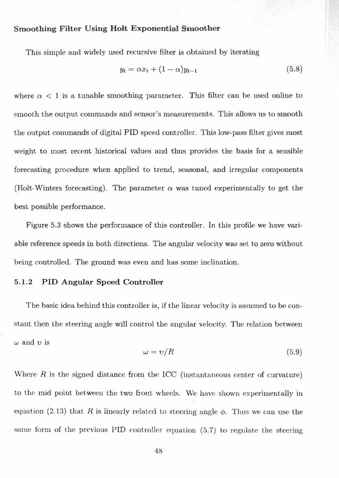
Figure 5.3 shows the performance of this controller. In this profile we have vari­

able reference speeds in both directions. The angular velocity was set to zero without

being controlled. The ground was ev n and has om in lination.

5.1.2 PIn Angular Speed Controller

The basic id a behind this controller is, if th linear v I ity is . urn d to b c n­

stant then the teering angle will control the angular v locity. Th r lation b tw n

wand v is w = viR (5.9)

Wh re R is the signed distance from the ICC (in tantan ous nter of curvature)

to th mid point between the two front wheel. We hay shown -xp rimentally in

equation (2.13) that R is linearly relat d to steering angle cPo Thus we can u e the

same form of the previous PID controller equation (5.7) to r gulat the steering

4

Measured and Reference linear veloclty

801--r---r---~--:;::=:::;:;=r:::::;:;:=::=:::;::C;=:;-1 : - Meaaured lnear velocity : - Reference linear Y8loc

. .60 . ................................. .

· . . .40t---.~t-7"r1"' ~. : ~ : : . · . . . .· . . . .· . . . .· . . . .· . . . .. , . .· . .· . .· . .20 ~ ~ ·4-.,.....;Pr#t.H : : ~ .

., .,.., . ... . . .. . . · .· .· .· . · .o , ;. . •••• , ••••••• :•••••••••••••• ••••••••••••.•• t •••••••••••• · .· .· .

· .-20 : : :.~--lI~~ rlHIrPrl'tA~ ... . ...... · .

-40 : ~ ; ~

· . .· .

-601....-__-..L. ..!- L-__-..L. -'-- L.-__~

o 10 20 30 40 50 60 70 t(Sec)

Figure 5.3: Measured and reference velocity

commands instead. One important parameter to consider is the sampling time. The

sampling time is limited by the ste ring rvo r pon tim (i., th ampling tim

can not be smaller than steering rvo re pon e tim). Th r pon tim of th

servo is constant at no load but it varie according to the whe l-ground friction. Th

design of the PIn controller will be for a nominal value of v b caus w is coupl d with

v as in equation (2.19). The angular speed controller as ume v icon tanto This

problem is eliminated by having a dynamic Pill gains. In other word ,th PIn gain

will vary based on the value of desired linear velocity. We used the the sam teps

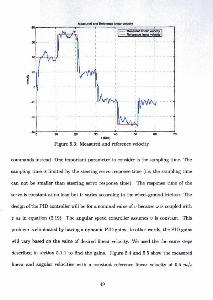
described in section 5.1.1 to find the gains. Figure 5.4 and 5.5 show the measured

linear and angular velocities with a constant reference linear velocity of 0.5 m/s

49

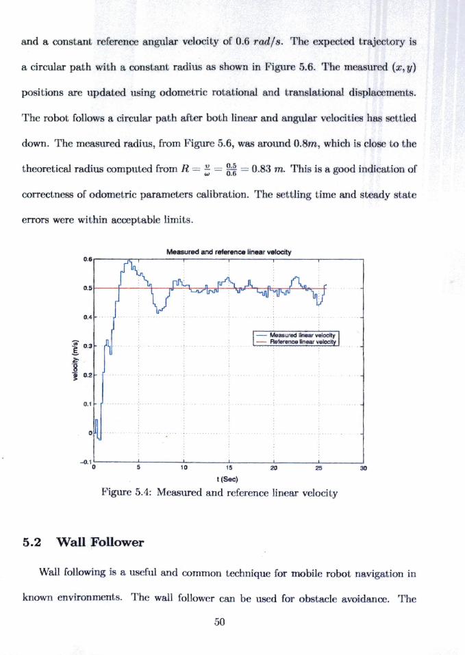
and a con tant r fer nc anglllar v loeiL of 0.6 radls. Tb xp t d Lraj cLory i

a circular path witb a consLan radiu as hown in I'igur 5.6. Th m ur d ( ,y)

po Won are updat d using odometri ro alional and tran lational di pIa m nt .

The robot follow a circlllar paLh aft r botb lin ar and angular v 10 iLi h eLL! d

down. The measured radiu ,from igure 5.6, was around O. m whi b i clo to Lh

theoretical radius computed from R = ~ = g:~ = 0.83 m. Thi i a good indicati.on of

correctness of odom Lric paramet rs caUbration. Th- ULing tim and Leady tat

errors were within acceptable HmiLs.

Measured and reference linear velocity 0.6.----;r-,--------,,--------,r-------.------.----,

0.4

- Measured "near velocny - Reference "near veloc ! 0.3 .

~

'Sl 0.2

0.1

o

-o.10:-----:5~---Jl:-0 ---...J'------1-----'-25----..J 15 20 30

t (Sec)

Figure 5.4: M asured and reC r nc lin ar velociLy

5.2 Wall Follower

Wall following i a useful and common L chni.que for mobile robot naviga ion in

known environm nts. The wall follower can be used for ob tad avoidance. Tb

50�

Measured and reference angular velocity 0.8r---,---......---r----;==::;;r==::;::::::;:::r:::;::::;:::;-i

:.0.7

Ii) 0.5

l .~ 0.4 •••.••..•••••••••• - •••• I' .•••••••••• • •••••• , ••••• 0 •••" ••••••••

~ ~ Iii 0.3 .. . .. : .. . " :­ . '3 g' < 0.2

0.1

o

-0.1 0 5 10 15 20 25 30

t (Sec)

Figure 5.5: Measured and reference angular velocity

execution of a planed path can be prevented by unexpected obstacle. When the

path can not be replanned, a imple strat gy con i t in following ~h c ntour of th

obstacle by using distance sensors [17]. The common nor u ed for w II [oUowing

is an ultrasonic transducer [28],[3]. In our impl m ntation , tb IR s n or w r m­

ployed for measuring the di t~ce to wall. A imple PID controll r was impl ment d

to achieve wall following.

5.3� Obstacle avoidance

Obstacle avoidance is an important behavior in autonomous v hicle. Th re are

many techniques to implements obstacle avoidance.. One of the olutions is to use

a potential field. In this approach, the obstacles are modeled as carrying electrical

charges. The robot is modeled as a charged point having the same charge as obstacles

51�

(X,y) Trajectrory Path 2

...• ·0 ...1.8

1.6

. I - Trajeclrory Path I 1.4

1.2

I >0­

0.8

0.6

0.4

0.2

O'----..l------'-------l---::::---'------'-------' -1 -0.5 0 0.5

X (m)

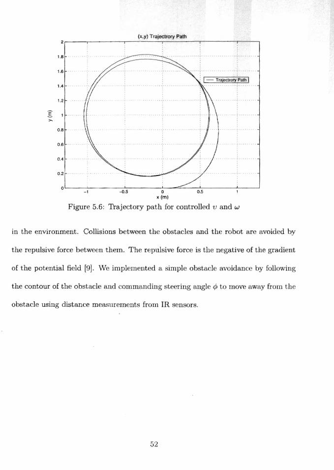
Figure 5.6: Trajectory path for controlled v and w

in the environment. Collisions between the obstacles and the robot are avoided by

the repulsive force between them. The repulsive force is the negative of the gradient

of the potential field [9}. W implem nted a impl ob tacl avoidan by fall wing

the contour of the obstacle and commanding te ring angl ¢ t mov way fr m th

obstacle using distance measurements from IR en ors.

52�

Chapter 6� Navigation Control and Localization�

This chapter de rib a localization m thod for outdoor 11 vio-ation u ing x-

tended Kalman (EKF) tilt r which fus odom try input 1 CPS and omp m a­

surernents.

6.1� Introduction

In this section, we discuss the effectivene of our designed robot by te ting 10 al­

ization algorithm using Kalman filter. Determining the robot location from physical

sensors has been referred to as [6] " the most fundamental problem to providing

the mobile robot with autonomous capabilities." Because of GPS position fixe are

inaccurate and at times may not be available, other navigation aids are used in con­

junction with GPS to enhance system performance. Dead reckoning sensors can not

be used alone for indefinitely long p riods, ince rrors grow without bound. Th y

accurately measure chang s in a v hid ' position ov r hort tim (can b us d al n

when GPS fixes becorn unavailabl for short p riods). The natur of th errors in

GPS position fixes is somewhat differ nt than that of the errors in d d r koning.

The errors appear in GPS position fixes and the errors in dead r ckoning ar ompl­

mentary in nature. Proper fusion of the GPS position fixes with th d ad re koning

sensor data can take advantage of the omplementary errors producing positioning

performance bett r than either type of data alone [1J.

There are a few example of. autonomous outdoor navigation robot and most

of them are costly re arch prototype . Another xarnple is given [24] but it u e a

53�

Laser canner which as urn prior knO'li I dg about th nviromn nt m r

set of sensors (Laser s ann r L 18220 and in rtial pI tform D U-6 ) u d in b t

experiment are very exp n ive. In [25] and [24] th ATRV-Jr platform manufa tur d

by iRobot used in the experiment I v r xpen iv ompar d to th 0 t of our

platform.

Outdoor environments are very difficult to work with b cau knowl dg , and th

terrain characteristics may not be available. The sonar, IR, or L r ann r u d f r

localization in indoors become useless in outdoors, though th y might still b 1.1 ed

as bumpers for obstacle avoidance. The next section explains how the localization

problem is solved.

6.2 Odometric Kalman Filter

Kalman filters have been efficiently used for state estimation. A common filter

type, is the odometric filter where r ading from th adorn try y t m n th rob t

are used together with the g om try of the robot mov m nt as a mod I f th r bot.

In order to be able to use the Kalman filter the proces model in quation (2.2) ne d

to be discretized first and then lineariz d. The di cr tiz d proc mod 1is xplain d

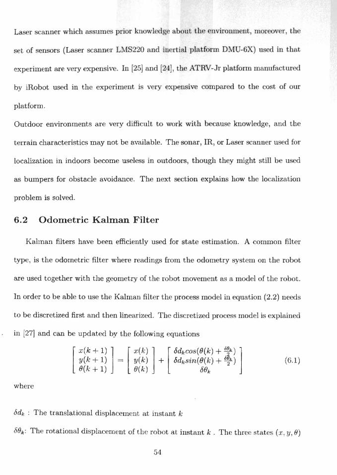
in [27] and can be updated by th following equation

x(k + 1) ] [ X(k)] [ e5dkcos(B(k) + t) ]'y(k + 1) . = ,y(k) + e5dksin(B(k) + ~) (6.1)

[ B(k + 1) O(k) , e5Bk

where

c5dk : The translational displacement at instant k�

e5Bk : The rotational di plac ment of the robot at instant k. Th three tates (x, y, B)�

54�

constitute the pro tat v tor. B on id ring 8dk and 8Bk input u(k) w(k)

system noise, and '"'((k) input noi e w r writ th nonlin r fun tion in quati n

(6.1) as:

x(k + 1) = f(x(k), u(k)' w(k), '"'((k)) (6.2)

The system and input noi e are assumed to be Gau ian with z ro m an and th ir

covariance matrices Q(k) and r(k) respectively (i.e. w(k) N(O, Q(k)),'"'((k) rv rv

N(O, r(k)) ).

An extended Kalman filter can be designed using the system mod 1in equation(6.1).

Denoting B(k) +~ as cp and linearizing the process model we get the following yst m

A and input G matrices

(6.3)

(6.4)

(6.5)

cos(cp) G(k + 1, k) = sin~cp) (6.6)

[

The measurements z(k) is expres d as:

z(k) = C(k)x(k) + v(k) (6.7)

Where v(k) is the measurement Doi e and it is assumed to he Gau sian with Z 1'0

mean and covarianc matrix R (i.e. v(k) N(O, R(k») ),rv

55�

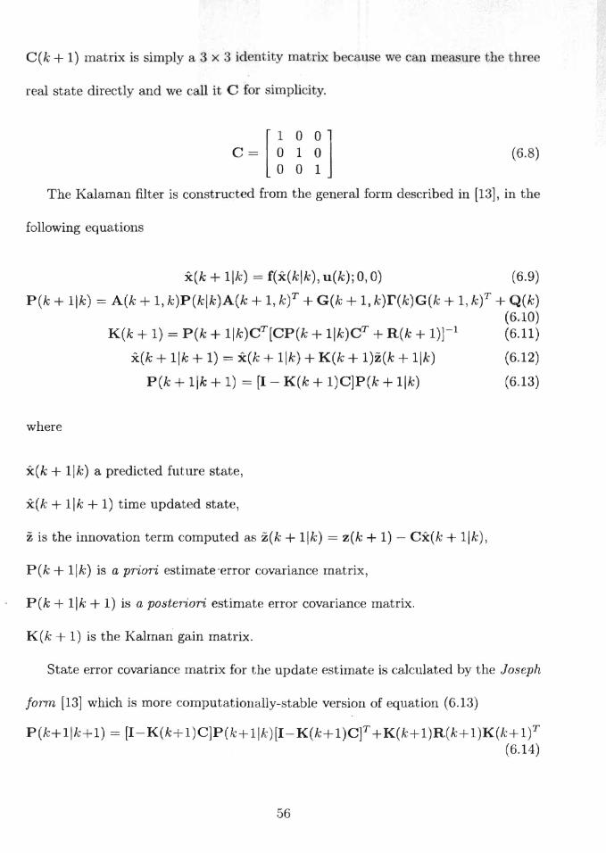
C(k + 1) matrix i simpl a 3 x 3 id n it matrix b w n m ure h thr

real state directly and w call it C for impli ity.

1 0 0]C = 0 1 0 (6.8)

[ 001

The Kalaman filter is construct d from the gen ral form d rib d in [13], in th

following equations

x(k + 11k) = f(x(klk), u(k); 0, 0) (6.9)

P(k + 11k) = A(k + 1, k)P(klk)A(k + 1, kf + G(k + I, k)r(k)G(k + 1, kf + Q(k) (6.10)

K(k + 1) = P(k + llk)CT[CP(k + llk)CT + R(k + l)r1 (6.11)

x(k + 11k + 1) = x(k + 11k) + K(k + l)z(k + 11k) (6.12)

P(k + 11k + 1) = [I - K(k + I)C]P(k + 11k) (6.13)

where

x(k + 11k) a predicted future state,�

x(k + 11k + 1) time updat d state,�

z is the innovation term comput d as z(k + 11k) = z(k + 1) - Cx(k + 11k),�

P(k + 11k) is a priori estimate"error covariance matrix,�

P(k + 11k + 1) is a posteriori estimate error covariance matrix.�

K(k + 1) is the Kalman gain matrix.�

State error covariance matrix for the update e timate is calculated by the Jo eph

form [13] which is more computationally- table version of quation (6.13)

P(k+lJk+l) = [1-K(k+l)C]P(k+llk)[I-K(k+ I)C]T +K(k+l)R(k+l)K(k+If (6.14)

56

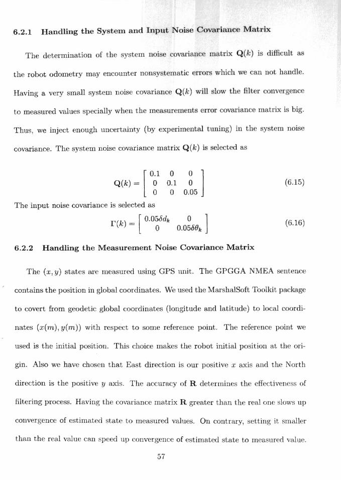
6.2.1 Handling the System and Input Nois Covariance Matrix

The determination of th ovarian rna rix Q(k) i diffi ult

the robot odometry may ncount r non y temati rr r whi h w an not 11 ndle.

Having a very small ystem nois covarianc Q (k) will low th flIt r

to measured values specially when the me urem nt nor covarian matrix i big.

Thus, we inject enough uncertainty (by xp rim ntal tuning) in th

covariance. The system noise covariance matrix Q(k) i 1 ct d as

0.1 (6.15)Q(k) = ~ [

The input noise covariance is selected as

r(k) = ,[ O.056dk 0 ] (6.16)0 O.050t'h

6.2.2 Handling the Measurement Noise Covariance Matrix

The (x, y) states are measured using GPS nnit. Th GPGGA NMEA nt n e

contains the position in global coordinates. We us d the MarshalSoft To lkit p kag

to covert from geodeti global oordinat s (longitud and latitude) t 10 1 coordi­

nates (x(m), y(m)) with resp ct to som referen point. Th r f r nc point w

used is the initial position. Thi choice makes the robot initial position at th ori­

gin. Also we have chosen that East dir ction is our po itive x axis and th orth

direction is the positiv y axis. The accuracy of R det rmines th ffe tiveness of

filtering process. Having the covariance matrix R gr ater than th real one slows up

convergence of estimat d stat to measured values. On contrary, setting it maller

than the real value can pe d up converg nce of estimat d state to measured value.

57�

In reality R i no stationar and h rr r in po ition ar ightl r lated. \M will

assume it is stationar for impli ity. Having can tan R during filt ring pr

may not result a good localization ac uracy a it v ri d p nding d p ndin n th

number of visible sat llite and iono ph ri audition. To hand I thi w n d to

have a dynamic R that chang based on GPS data quality. Th Diluti n Of Pr ­

cision DOP can tell about the quality of GPS dat . DOP i updat d b d on the

alignment, or geometry, of the group of atellites ( on tellation) from whi h 'ignal

are being received. We used this to modify the ubmatrix of R. How ver, th re

is no guarantee that the estimated state will converge to the actual state wh n the

measurements are not available for long time. For Heading angle m asur ment we

used both GPS and compass to give heading angle. Heading angle from GPS is

available at the GPRMC NMEA sentence. The GPS unit must be moving to get

accurate reading from GPS heading angle. The accuracy depends upon the speed

of the vehicle. It is very accurate at higher sp ds and 'ompl t ly fal wh n th

robot does not move. Ther fore, the heading angle m asur m nt from GPS ar

disregarded at very low speeds and th varian e of m ur d f:} i ill difi d bas d n

the speed of the robot. Fortunat ly, the compas has oppo it b havior. W will

switch between GPS and compas readings, how v r, the GPS will b th dominant

sensor for providing heading angle m asurements be ause the robot i moving rna t

of time. The heading submratix of R is updated by the varian e of th s nsor used

for measuring heading angle.

58�

6.2.3 Handling the Different Sampling Rat 5

The dead reckoning data i given at a higher fr qu n y (e r 200 Tn. e ond) , th n

the information availabl from CPS ( v r 1 econd) h n tim upd t and the

measurement update part operate at differ nt rat . W in orpar m ur m nt

when it is available. When th measur m nt i not availabl th pI' di t d futur

state and the a priori state error covariance are u d a po teriori tat timat

and state error covariance for the next iteration.

6.3� Navigation Controller

This section describes different controllers that us the e timated po ition giv n

by EKF to reach a desired target position. This problem is solved using different

controllers [2].

6.3.1 Target Acquisition Using Leader Following Approach

We use the leader following control algorithm to r a had sir d d stinatiol1 (i. .,

the leader robot is at reset). We us a velo ity ontrolled v hi 1 that u s th

kinematic model only. The convergenc to command d v locity an be guar nt d

by our previous PID v locity controller. The formation control law w I' d riv d

using input-output feedback linearization [15]. The kinematics of both I ad rand

follower are represented by the unicycle model giv n in equation (2.2). We on id r

two robots shown in Figure 6.1, where Vj and Wj are the linear and angular v 10 iti s

of the follower at midpoint on the front axle.

We� will describe the kinematic controller for leader following, present d in [8].

59�

R·I Vi' O>i

'-'--" y \,8.

, I ,.

X Figure 6.1: Two robots in a leader following configuration.

The leader will benxed at the d tination point with both lin ar and angul r v 10 i-

ties are set to zero. By applying input/output lin arization t g nerat a ntr llaw

that gives an exponentially onv rgent solution in th vari hI iij and 'l/Jij w g t

Vj = k1(j cos "'Yij - iij in "'Yij (k2~j + Wi) + Vi 0 (3ij (6.17)

1 - -Wj = dlkliij sin "'Yij + iij cos "'Yij(k21/Jij + wd + Vi sin (3ij] (6.18)

where

d is an offset distance to the midpoint of front axle P j of the robot, and k1 and k2

are the user selected control gains. The closed-loop linearized system b come

60�

- -

ij = k2 ij (6.19)

Because we are using Cart ian oordinat I \. an omput u in lT

/3 = atan2(ii; - Yi i - Xj) (6.20)

where

Xj = Xj + dcose, Yj = Yj + d in e,

By setting the angular and linear speed of the lead r at z w, th control input

become Vj = k1lij cos 'Yij - lij sin 'Yij k2'l/Jij (6.21)

1 - -Wj = d[k1lij sin 'Yij + iij cos 'Yij k2'l/Jij] (6.22)

6.3.2 Experimental Results

In this experiment we initiated the robot at (x(O), yeO), 11(0» = (0,0,0) and

set the target position at (Xt> yd = (20,9). Th po ition was timat d using th

Kalman filter. We do not have a ground truth for r al traj tory trav r d by th

robot, however, the final position reached by th rohot w within 1m rr r from th

position of the target. Figure 6.2 shows the trajectori cornput d from stirnat cl

state of Kalman filter, measured po ition from GPS, and odometric upd t d po ition.

The odometric trajectory is updated using the kin matic mod I d scrib d in quation

(6.1) without taking the advantage of GPS and compass. Th odometric tat i

correct in the beginning) however, in th middle of the path the rror ac umul ted

to give completely wrong y position at the end. The GPS reading are corr ct and

within the device accuracy. The e timated po ition agree with the ob rvation that

61�

tru robo follow a traighl. line toward l.h ar l..

EstImated, odometry (process),and Measured(GPS) trajectortes 12 ,--....,---,.--.,.---,---,----r----,,---....,---,.----,

10

8 .

6

4. • .••...••••••. /

2 ...

o....--..------~

- estimated polltlon - Position updated using odometry - Position lrom GPS

-2 L~L.____JI__----l_--1_--l.____=:::::r:=::::t=:::=r:==:::::i;=__~ o 2 4 6 B to 12 14 16 16 20

x(m)

Figure 6.2: Estimated, measured and proc s traj clori

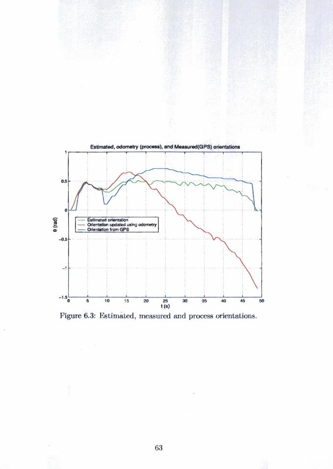
To analyze tbis xperirnent in mor d tail, w pioU d th h adin)" an 1 ri. v n

by timated tate (Kalman filter d), m ur d hading angl ( P and omp )

and odom try (proce only withoul. incorpora ing any m UT m. nts) as hown in

Figure 6.3. As we ee from Figure 6.3) the ori ntation angl from b lh odom ryand

estimated state wer almost the sam in th b ginning. Th ill asur d hading anglo

provides corrections for the filter once tb lin ar spe d is in p d. Th stimal d

heading angle takes the advantag of tb correct m. asur m nL while odom tri'tat

heading angt accumulate rrors to reacb completely incorr cl final valu .

62�

Estimated. odornetry (process), and Measured(GPS) orientations

0.5

- Estlmated orientation - Or1entation updated using odOmelry - Or1entation from GPS

-0.5

-1

~_---'-Ul __---L__...L.__....L.- .L.-_---JL...-_......J.. --L ....L.-_-.J__ __ __

o 5 10 15 20 25 30 35 <10 45 50 t (s)

Figure 6.3: Estimated, measured and pro

63�

----------- - --

Chapter 7� Conclusion and Future Work�

7.1 Concluding Remarks

This thesis has de cribed th d v loping of a modul r mobil t tb db· mod­

ifying the standard chassis of a omm r ial in xpen iv R/ tru k. Th v hi 1 i

equipped with a suite of ensor to op rate autonomou ly. Th

cludes IR, odometer, GPS, and vision y t m. Th onbo rd not book along with

the multifunction acquisition card provided a computational pow r for s nsory data

processing.

The kinematic model for the vehicle was derived and it was shown that th

unicycle model is a valid model for the vehicle under some conditions. Tools for robot

control have been designed and implemented and their performance is promising. A

control archite ture utilizing obje t ori nt d multi-thr ading was u d to

modularity.

Also we have demonstrated that good r suIts of loc lizati n ar obt in bi by

using only an inexpensive well alibrated d ad r ckoning s nsors and an in xp nsiv

commercial GPS unit. The target acquisition is achi v d by applying Input/Output

feed back linearized controller for leader following. Further exp rim nt 1r s arch an

be carried out using the de igned vehi Ie to verify th oreti al r suIt that hay b en

validated using only simulation.

64�

7.2 Future Work

There are some modification n d t b don to g tab tt I' P r£ I'm n f th

robot.

7.2.1� Hardware Modifications

The following ar some suggestions for modifi tion on hardwar .

•� Adding a gyro to measure angular velocity so we can avoid non y temati rror

in odometry.

•� Building power monitoring system to give the statu of remaining pow I' in

batteries.

7.2.2� Software Modifications

Here are some suggestions for software improvement

•� Devlop the communication network betw n vehi 1 s. On pos ibl olution i

to use . Net.

•� Improving real-time performance by adding I' aI-time xtensions.

•� Impl menting more functions that take the advantag of vision unit.

7.2.3 Localization Algorithm Improvement

Though the localization algorithm using Kalman filt I' works fine, th following

suggestion can improve the filter performance

•� Extending the state of the filter to includ both angular and linear velocity.

65�

• Improving m asur m n a cur

the CPS unit and compass pI'

y b

i ion.

u in high I' pr i ion d vi

• Extending th measurements vector of th

measured by a gyro.

tilt I' to in Iud angular I ity

66�

Company Product Address Telephone Web Site

Company Product Address Telephone Web Site

Company Product Address Telephone Web Site

Company Product Addre Telephone Web Site

Company Product Address Telephone Web Site

Company Product Address Telephone Web Site

Company Product Address

Appendix A� Hardware Sources�

Tamiya Am rica, Inc. RC car chasis 2 Orion Aliso Vi jO,CA 92656-4200 1-800-TAMIYA-A http://www.tamiyausa.om

Sony Electroni sIne. Notebook Sony VAIO SRX SRX99 1 Sony Drive MD TA3-12 Park Ridg , N w J r y 07656 (877) 865-S0NY(7669) http://www.sonystyle.com

Sharp Electronics Corporation [U.S.A.] JR Distance measuring sensor 1300 Naperville Drive, Romeoville, IL 60446 1-800-237-4277 / 1-800-BE SHARP http://www.sharp.co.jp

National Instruments Corporation I DAQCard-6024E for PCMCIA and CB-68LPR DAQ

11500 N Mopac Expwy Au tin, TX 7 759-3504 1-512-683-0100 http) /www.nLcom

Agilent Technologies, Inc. Reflective optical surface mount neod rand odewh Is 395 Page Mill Rd.P.O. Box 10395 Pal Alto, A 94303 1 650 752-5000 http://wwwagilent.com/emi ondu tor

Hitec RCD USA, Inc. Servos 12115 Paine St. Poway CA, 92064 1-858-748-6948 http://www.hitecrcd.com

Digi-Key Electronic component· 701 Brooks Avenu South Thief River Falls, M 56701

G7�

Telephon Web Site

Company Product Addre s Telephone Web Site

Company Product Address Telephone Web Site

Company Product Address Telephone Web Site

Company Product Address Telephone Web Site

Company Product Address Telephone Web Site

1-800-DIGI-I EY http://www.digik . om

Thale avigation lagellan GPS

471 El Camino R al Santa Clar CA 95050-4300 1-408-615-5100 http://www.magellangps.om

Scott Edwards Electronic In . Serial Servo Controll 1's (SSC ) 1939 S. Frontage Rd. #F, Si rra Vista, AZ 85635 1-520-459-4802 http://www.seetron.com

Tower Hobbies RC car upgrade components PO Box 9078 Champaign, IL 61826-9078 1-800-637-6050 www.towerhobbies.com

Robson Company, Inc. 1655 Analog Compass Sensor 227 Hathaway St. E. Girard, PA 16417 1-814-774-5914 http://www.dinsmore n or·. m

Novak Electronics, Inc. Electronic speed control 18910 Teller Avenue Irvin, CA 92612 1-949-833-8873 http://www.teamnovak.com

68�

I

References�

1.� E. Abbott, D. Pow 11 Land-vebi I navigation u ing GP Pro .IEEE vol. 87 I ue: 1 Jan. 1999 pp. 145 - 162.

2.� M. Aicardi, G. Casalino, A. Bic bi, A. B Ie rino, Cl d loop t ring of unicycle like v hicles via Lyapunov t bniqu ,IEEE Roboti & Automation Magazine, vol. 2 Is ue: 1 I March 1995, pp. 27 - 35.

3.� A. Bemporad, M. Di Marco, A. Tesi, "Wall-following ontr 11 r for n r-b ed mobile robots", in Proc. IEEE Con! Decision and Control, D c. 1997 pp. 3063 - 3068.

4.� R. Bishop, "Intelligent vehicle applications worldwide", Int lUg nt Systems IEEE, , vol.15 Issue: 1 , Jan.-Feb. 2000, pp.78 - 81.

5.� J. Borenstein, H. R. Everett, and 1. Feng contributing authors: S.W. L e and R. H. Byrne, WheTe am I? sensors and methods for mobile robot positioning, April 1996.

6.� I.J. Cox, "An experiment in guidance and navigation of an autonomou robot vehicle", IEEE Transactions on Robotics and Automation" voL 7 Issu : 2, April 1991, pp. 193 - 204.

7.� A. K. Das, R. Fierro, V. Kumar, J. P. Ostrowski, J. Spletzer, and C. J. Taylor, "A vision based formation control framework, " IEEE Transactions on Robotics and Automation, voL 18, no. 5, Oct. 2002, pp. 813 - 25.

8.� J. Desai, J.P. 0 trowski, and V. Kumar, " Controlling formation of multipl mobile robots", in Proc. IEEE Int rnational Confi rence on Roboti and Au­tomation, Leuven, Belgium, May 1998, pp. 2864 - 2869.

9.� G. Dudek, M. Jenkin, Computational principle of mobil roboti ,Cambridg University press 2000.

10.� G.D. Dunlap, H.H Shufeldt, "Dutton's Navigation and piloting", Naval in titut press, pp.557 - 579.

11.� L Erkmen, A.M. Erkmen, F. Matsuno, R. Chatterje , T. Karn gawa, "Snak robots to the rescue! ", Robotics & Automation Magazin , IEEE, vol. 9, Sept. 2002 pp. 17 - 25.

12.� R. Fierro and E. Edwan, " The OSU multi-vehicle coordination t tbed", The 2002 45th Midwest Symposium on Circuits and Systems , vol. 3 , Augu t 2002,pp. 41 - 44.

13.� R. Grover, B. Patrick, Y. C. Hwang, Introduct'ion to random signal and applied Kalman filtering: with MATLAB ex rcises and solutions, 3rd Ed., John Wiley Son Inc., 1997.

69�

14.� R. D. Hem, Automotiv ultrasonic headway control for a s aled robotic ar , Th is, Virginia Pol chnlc In titut nd ta Univ r ity 2001.

15. A. Isidori,� Nonlinear Control Sy terns Spring r- V< rlag Lond n rd dition 1995.

16.� J. Laumond, "Robot Motion Planning and ontrol , Spring r 199

17.� J.C. Latombe, "Robot motion Planning", KAP, Bo ton, 1991.

18.� "Measurment and Automation CATALOG 2003', ATIONAL INSTUR­ME TS, pp.772 - 773.

19.� P.J. McKerrow, D. Ratner, "Calibrating a 4-wh 1 mobil robot', in Proc. IEEE/RSJ International Conference on Intelligent Robots and Sy tem, vol.1 , Oct. 2002 pp. 859 - 864.

20.� P. Mellodge, "Feedback control for a path following 'rObotic car' , The is, Virginia Polytechnic Institute and State University, 2002.

21.� N. Miyake, T. Aono, K. Fujii, Y. Matsuda, S. Hatsumoto, "Poition estimation and path control of an autonomous land vehicle", in Proc. IEEE/RSJ, Interna­tional Conference on Intelligent Robots and Systems, vo1.2 , Sept. 1997, pp. 690 - 696.

22.� S. Murata, T. Hirose, "Onboard location system using real-time image process­ing for self navigating vehicle", IEEE Transactions on Industrial Eelectronics, vol. 40 Issue: 1 , February 1993, pp. 145 - 154.

23.� N. S. Nise, Control Systems Engineering, 2nd Ed., Addi n-W ly, Y, 1995.

24.� S. Panzieri, F. Pascuc i, G. Ulivi, " An outdoor navigation y t m u ing PS and inertial platform" , IEEE/A SME Transactions on Mechatronics, vol. 7 Is u 2 , Jun 2002, pp. 134 - 142.

25.� R. Thrapp, C. Westbrook, D. Subramanian, "Robust 10 alization Igorithm f r an autonomous campus tour guide" , in Proc. IEEE International Conferenc on Robotics and Automation, vol. 2 , 2001 pp. 2065 - 2071.

26.� S. Thrun, M. Bennewitz, W. Burgard, A.B. Cremers, F. D lla rt, D. Fox, D. Hahnel, C. Rosenberg, N. Roy, J. Schulte, D. S hulz, "MINERVA: a s cond­generation museum tour-guide robot", in Proc. IEEE International Confer, nce on Robotics and Automation, vo1.3 , May 1999 pp. 1999 - 2005.

27.� C.M. Wang, "Location stimation and uncertainty analy is for mobile robots", in Proc. IEEE International Conference on Robotics and Automation, Apr 19 8 pp. 1231 - 1235.

70

28.� T. Yata, L. I I man S. Yuta Wall f llov ing u ing an I inform ti n m ur d by a single ultr onie tran du r in Pro. IEEE Int rnational Confer n on Robot Automatation vo1.2 fa 199 pp. 15 0 - 1596.

29.� http://www.evoluion.om

30.� http://www.u.aibo.com

31.� http://www.faqs.org/faq Ir altime-computing/faq

32.� http://www.irohot.com

33.� http://gps.faa.gov/Programs/WAAS/waas.htm

34.� http://www.gpsinformation.org/dale/nmea.htm

35.� MarshallSoft Computing, http://www.marshallsoft.com/mgc4c.htm

36. MSDN� Library, http://msdn.microsoft.com/libraryIdefault.asp?url=/librarylen­us/ dnxpembed/html/hardrealtime.asp

37. Venturcom, Inc. http://www.vci.com/

71�

d ...

VITA�

EZZALDEEN EDWAN�

Candidate for the degree of�

Master of Science�

Thesis: DESIGN OF A MODULAR AUTONOMOUS ROBOT VEHICLE

Major Field: Electrical EngineeIing

Biographical:

Personal Data: Born in Rafah, Palestine, On November 17, 1973.

Education: Received Bachelor of Science def,'Tee in lectrical engineering from Birzeit University, Birzeit, Palestine in March 1997. Completed the requirements for the Master of Science degree with a major in Electrical Engineering at Oklahoma State University in (August, 2003).

Experience: Employed as lecturer engineer by Palestine Technical College, 1997 to 2001.

Professional MemJJerships: Institute of Electrical and Electronic Engineers, Phi Kappa Phi.