Design of evolutionary methods applied to the learning of Bayesian network structures Thierry BROUARD, Alain DELAPLACE, Muhammad Muzzamil LUQMAN, Hubert CARDOT and Jean-Yves RAMEL University François Rabelais France 1. Introduction Bayesian networks (BN) are a family of probabilistic graphical models representing a joint distribution for a set of random variables. Conditional dependencies between these variables are symbolized by a Directed Acyclic Graph (DAG). Two classical approaches are often encountered when automatically determining an appropriate graphical structure from a database of cases. The first one consists in the detection of (in)dependencies between the variables (Cheng et al., 2002; Spirtes et al., 2001). The second one uses a scoring metric (Chickering, 2002a). But neither the first nor the second are really satisfactory. The first one uses statistical tests which are not reliable enough when in presence of small datasets. If numerous variables are required, it is the computing time that highly increases. Even if score-based methods require relatively less computation, their disadvantage lies in that the searcher is often confronted with the presence of many local optima within the search space of candidate DAGs. Finally, in the case of the automatic determination of the appropriate graphical structure of a BN, it was shown that the search space is huge (Robinson, 1976) and that is a NP-hard problem (Chickering et al., 1994) for a scoring approach. In this field of research, evolutionary methods such as Genetic Algorithms (GA) (De Jong, 2006) have already been used in various forms (Acid & de Campos, 2003; Larrañaga et al., 1996; Muruzábal & Cotta, 2004; Van Dijk, Thierens & Van Der Gaag, 2003; Wong et al., 1999; 2002). Among these works, two lines of research are interesting. The first idea is to effectively reduce the search space using the notion of equivalence class (Pearl, 1988). In (Van Dijk, Thierens & Van Der Gaag, 2003) for example the authors have tried to implement a genetic algorithm over the partial directed acyclic graph space in hope to benefit from the resulting non-redundancy, without noticeable effect. Our idea is to take advantage both from the (relative) simplicity of the DAG space in terms of manipulation and fitness calculation and the unicity of the equivalence classes’ representations. One major difficulty when tackling the problem of structure learning with scoring methods – evolutionary methods included – is to avoid the premature convergence of the population to a local optimum. When using a genetic algorithm, local optima avoidance is often ensured by preserving some genetic diversity. However, the latter often leads to slow convergence and difficulties in tuning the GA parameters. 2

Welcome message from author
This document is posted to help you gain knowledge. Please leave a comment to let me know what you think about it! Share it to your friends and learn new things together.
Transcript
Design of evolutionary methods applied to the learning of Bayesian network structures 13
Design of evolutionary methods applied to the learning of Bayesian network structures
Thierry Brouard, Alain Delaplace, Muhammad Muzzamil Luqman, Hubert Cardot and Jean-Yves Ramel
0
Design of evolutionary methods applied to thelearning of Bayesian network structures
Thierry BROUARD, Alain DELAPLACE, Muhammad MuzzamilLUQMAN, Hubert CARDOT and Jean-Yves RAMEL
University François RabelaisFrance
1. Introduction
Bayesian networks (BN) are a family of probabilistic graphical models representing a jointdistribution for a set of random variables. Conditional dependencies between these variablesare symbolized by a Directed Acyclic Graph (DAG). Two classical approaches are oftenencountered when automatically determining an appropriate graphical structure from adatabase of cases. The first one consists in the detection of (in)dependencies between thevariables (Cheng et al., 2002; Spirtes et al., 2001). The second one uses a scoring metric(Chickering, 2002a). But neither the first nor the second are really satisfactory. The firstone uses statistical tests which are not reliable enough when in presence of small datasets.If numerous variables are required, it is the computing time that highly increases. Even ifscore-based methods require relatively less computation, their disadvantage lies in that thesearcher is often confronted with the presence of many local optima within the search spaceof candidate DAGs. Finally, in the case of the automatic determination of the appropriategraphical structure of a BN, it was shown that the search space is huge (Robinson, 1976) andthat is a NP-hard problem (Chickering et al., 1994) for a scoring approach.
In this field of research, evolutionary methods such as Genetic Algorithms (GA) (De Jong,2006) have already been used in various forms (Acid & de Campos, 2003; Larrañaga et al.,1996; Muruzábal & Cotta, 2004; Van Dijk, Thierens & Van Der Gaag, 2003; Wong et al., 1999;2002). Among these works, two lines of research are interesting. The first idea is to effectivelyreduce the search space using the notion of equivalence class (Pearl, 1988). In (Van Dijk,Thierens & Van Der Gaag, 2003) for example the authors have tried to implement a geneticalgorithm over the partial directed acyclic graph space in hope to benefit from the resultingnon-redundancy, without noticeable effect. Our idea is to take advantage both from the(relative) simplicity of the DAG space in terms of manipulation and fitness calculation andthe unicity of the equivalence classes’ representations.
One major difficulty when tackling the problem of structure learning with scoring methods –evolutionary methods included – is to avoid the premature convergence of the population toa local optimum. When using a genetic algorithm, local optima avoidance is often ensured bypreserving some genetic diversity. However, the latter often leads to slow convergence anddifficulties in tuning the GA parameters.
2
Bayesian Network14
To overcome these problems, we designed a general genetic algorithm based upon dedicatedoperators: mutation, crossover but also a mutual information-driven repair operator whichensures the closeness of the previous. Various strategies were then tested in order to find abalance between speed of convergence and avoidance of local optima. We focus particularlyonto two of these: a new adaptive scheme to the mutation rate on one hand and sequentialniching techniques on the other.
The remaining of the chapter is structured as follows: in the second section we will definethe problem, ended by a brief state of the art. In the third section, we will show how anevolutionary approach is well suited to this kind of problem. After briefly recalling the theoryof genetic algorithms, we will describe the representation of a Bayesian network adapted togenetic algorithms and all the needed operators necessary to take in account the inherentconstraints to Bayesian networks. In the fourth section the various strategies will then bedeveloped: adaptive scheme to the mutation rate on one hand and niching techniques on theother hand. The fifth section will describe the test protocol and the results obtained comparedto other classical algorithms. A study of the behavior of the used strategies will also be given.And finally, the sixth section will present an application of these algorithms in the field ofgraphic symbol recognition.
2. Problem settings and related work
2.1 SettingsA probabilistic graphical model can represent a whole of conditional relations within a fieldX = {X1, X2, . . . , Xn} of random variables having each one their own field of definition.Bayesian networks belong to a specific branch of the family of the probabilistic graphicalmodels and appear as a directed acryclic graph (DAG) symbolizing the various dependencesexisting between the variables represented. An example of such a model is given Fig. 1.
A Bayesian network is denoted B = {G, θ}. Here, G = {X, E} is a directed acyclic graphwhose set of vertices X represents a set of random variables and its set of arcs E represents thedependencies between these variables. The set of parameters θ holds the conditional proba-bilities for each vertices, depending on the values taken by its parents in G. The probabilityk = {P(Xk|Pa(Xk))}, where Pa(Xk) are the parents of variable Xk in G. If Xk has no parents,then Pa(Xk) = ∅.The main convenience of Bayesian networks is that, given the representation of conditionalindependences by its structure and the set θ of local conditional distributions, we can writethe global joint probability distribution as:
P(X1, . . . , Xn) =n
∏k=1
P(Xk|Pa(Xk)) (1)
2.2 Field of applications of Bayesian networksBayesian networks are encountered in various applications like filtering junk e-mail (Sahamiet al., 1998), assistance for blind people (Lacey & MacNamara, 2000), meteorology (Cano et al.,2004), traffic accident reconstruction (Davis, 2003), image analysis for tactical computer-aideddecision (Fennell & Wishner, 1998), market research (Jaronski et al., 2001), user assistance in
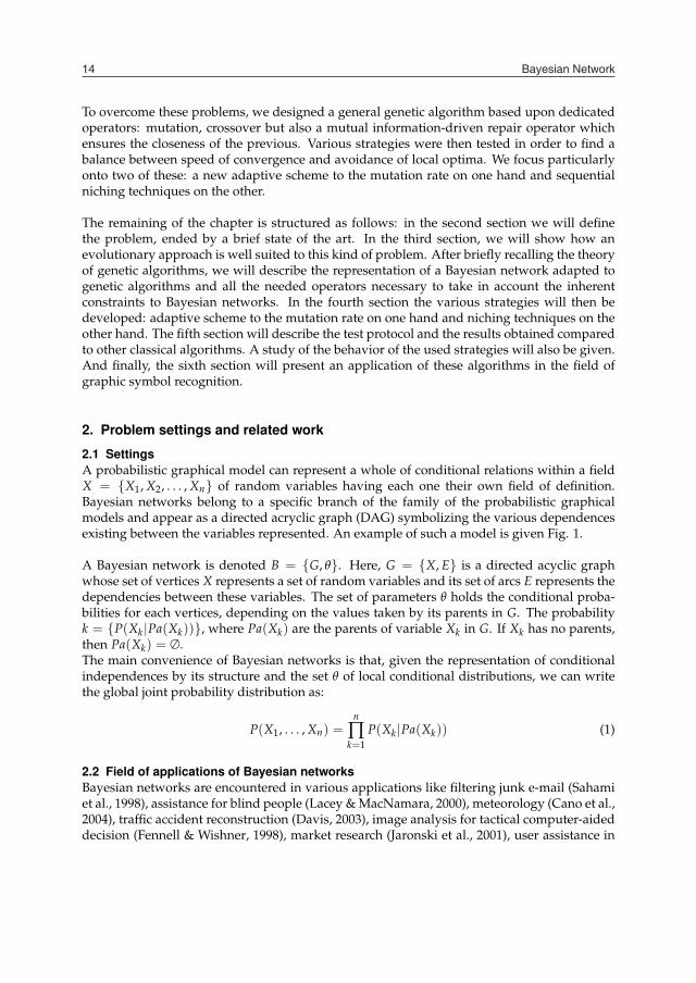
Fig. 1. Example of a Bayesian network.
software use (Horvitz et al., 1998), fraud detection (Ezawa & Schuermann, 1995), human-machine interaction enhancement (Allanach et al., 2004).
The growing interest, since the mid-nineties, that has been shown by the industry for Bayesianmodels is growing particularly through the widespread process of interaction between manand machine to accelerate decisions. Moreover, it should be emphasized their ability, incombination with Bayesian statistical methods (i.e. taking into account prior probabilitydistribution model) to combine the knowledge derived from the observed domain with aprior knowledge of that domain. This knowledge, subjective, is frequently the product ofthe advice of a human expert on the subject. This property is valuable when it is known thatin the practical application, data acquisition is not only costly in resources and in time, but,unfortunately, often leads to a small knowledge database.
2.3 Training the structure of a Bayesian networkLearning Bayesian network can be broken up into two phases. As a first step, the networkstructure is determined, either by an expert, either automatically from observations madeover the studied domain (most often). Finally, the set of parameters θ is defined here too byan expert or by means of an algorithm.
The problem of learning structure can be compared to the exploration of the data, i.e. theextraction of knowledge (in our case, network topology) from a database (Krause, 1999). Itis not always possible for experts to determine the structure of a Bayesian network. In somecases, the determination of the model can therefore be a problem to resolve. Thus, in (Yu et al.,2002) learning the structure of a Bayesian network can be used to identify the most obviousrelationships between different genetic regulators in order to guide subsequent experiments.

Design of evolutionary methods applied to the learning of Bayesian network structures 15
To overcome these problems, we designed a general genetic algorithm based upon dedicatedoperators: mutation, crossover but also a mutual information-driven repair operator whichensures the closeness of the previous. Various strategies were then tested in order to find abalance between speed of convergence and avoidance of local optima. We focus particularlyonto two of these: a new adaptive scheme to the mutation rate on one hand and sequentialniching techniques on the other.
The remaining of the chapter is structured as follows: in the second section we will definethe problem, ended by a brief state of the art. In the third section, we will show how anevolutionary approach is well suited to this kind of problem. After briefly recalling the theoryof genetic algorithms, we will describe the representation of a Bayesian network adapted togenetic algorithms and all the needed operators necessary to take in account the inherentconstraints to Bayesian networks. In the fourth section the various strategies will then bedeveloped: adaptive scheme to the mutation rate on one hand and niching techniques on theother hand. The fifth section will describe the test protocol and the results obtained comparedto other classical algorithms. A study of the behavior of the used strategies will also be given.And finally, the sixth section will present an application of these algorithms in the field ofgraphic symbol recognition.
2. Problem settings and related work
2.1 SettingsA probabilistic graphical model can represent a whole of conditional relations within a fieldX = {X1, X2, . . . , Xn} of random variables having each one their own field of definition.Bayesian networks belong to a specific branch of the family of the probabilistic graphicalmodels and appear as a directed acryclic graph (DAG) symbolizing the various dependencesexisting between the variables represented. An example of such a model is given Fig. 1.
A Bayesian network is denoted B = {G, θ}. Here, G = {X, E} is a directed acyclic graphwhose set of vertices X represents a set of random variables and its set of arcs E represents thedependencies between these variables. The set of parameters θ holds the conditional proba-bilities for each vertices, depending on the values taken by its parents in G. The probabilityk = {P(Xk|Pa(Xk))}, where Pa(Xk) are the parents of variable Xk in G. If Xk has no parents,then Pa(Xk) = ∅.The main convenience of Bayesian networks is that, given the representation of conditionalindependences by its structure and the set θ of local conditional distributions, we can writethe global joint probability distribution as:
P(X1, . . . , Xn) =n
∏k=1
P(Xk|Pa(Xk)) (1)
2.2 Field of applications of Bayesian networksBayesian networks are encountered in various applications like filtering junk e-mail (Sahamiet al., 1998), assistance for blind people (Lacey & MacNamara, 2000), meteorology (Cano et al.,2004), traffic accident reconstruction (Davis, 2003), image analysis for tactical computer-aideddecision (Fennell & Wishner, 1998), market research (Jaronski et al., 2001), user assistance in
Fig. 1. Example of a Bayesian network.
software use (Horvitz et al., 1998), fraud detection (Ezawa & Schuermann, 1995), human-machine interaction enhancement (Allanach et al., 2004).
The growing interest, since the mid-nineties, that has been shown by the industry for Bayesianmodels is growing particularly through the widespread process of interaction between manand machine to accelerate decisions. Moreover, it should be emphasized their ability, incombination with Bayesian statistical methods (i.e. taking into account prior probabilitydistribution model) to combine the knowledge derived from the observed domain with aprior knowledge of that domain. This knowledge, subjective, is frequently the product ofthe advice of a human expert on the subject. This property is valuable when it is known thatin the practical application, data acquisition is not only costly in resources and in time, but,unfortunately, often leads to a small knowledge database.
2.3 Training the structure of a Bayesian networkLearning Bayesian network can be broken up into two phases. As a first step, the networkstructure is determined, either by an expert, either automatically from observations madeover the studied domain (most often). Finally, the set of parameters θ is defined here too byan expert or by means of an algorithm.
The problem of learning structure can be compared to the exploration of the data, i.e. theextraction of knowledge (in our case, network topology) from a database (Krause, 1999). Itis not always possible for experts to determine the structure of a Bayesian network. In somecases, the determination of the model can therefore be a problem to resolve. Thus, in (Yu et al.,2002) learning the structure of a Bayesian network can be used to identify the most obviousrelationships between different genetic regulators in order to guide subsequent experiments.

Bayesian Network16
The structure is then only a part of the solution to the problem but itself a solution.
Learning the structure of a Bayesian network may need to take into account the nature of thedata provided for learning (or just the nature of the modeled domain): continuous variables– variables can take their values in a continuous space (Cobb & Shenoy, 2006; Lauritzen &Wermuth, 1989; Lerner et al., 2001) –, incomplete databases (Heckerman, 1995; Lauritzen,1995). We assume in this work that the variables modeled take their values in a discreteset, they are fully observed, there is no latent variable i.e. there is no model in the field ofnon-observable variable that is the parent of two or more observed variables.
The methods used for learning the structure of a Bayesian network can be divided into twomain groups:
1. Discovery of independence relationships: these methods consist in the testing proce-dures on allowing conditional independence to find a structure;
2. Exploration and evaluation: these methods use a score to evaluate the ability of thegraph to recreate conditional independence within the model. A search algorithm willbuild a solution based on the value of the score and will make it evolve iteratively.
Without being exhaustive, belonging to the statistical test-based methods it should be notedfirst the algorithm PC, changing the algorithm SGS (Spirtes et al., 2001). In this approach,considering a graph G = {X, E, θ}), two vertices Xi and Xj from X and a subset of verticesSXi ,Xj ∈ X/{Xi, Xj}, the vertices Xi and Xj are connected by an arc in G if there is no SXi ,Xj
such as (Xi⊥Xj|SXi ,Xj ) where ⊥ denotes the relation of conditional independence. Basedon an undirected and fully connected graph, the detection of independence allows us toremove the corresponding arcs until the obtention the skeleton of the expected DAG. Thenfollow two distinct phases: i) detection and determination of the V-structures1 of the graphand ii) orientation of the remaining arcs. The algorithm returns a directed graph belongingto the Markov’s equivalence class of the sought model. The orientation of the arcs, exceptthose of V-structures detected, does not necessarily correspond to the real causality of thismodel. In parallel to the algorithm PC, another algorithm, called IC (Inductive Causation)has been developed by the team of Judea Pearl (Pearl & Verma, 1991). This algorithm issimilar to the algorithm PC, but starts with an empty structure and links couples of variablesas soon as a conditional dependency is detected (in the sense that there is no identifiedsubset conditioning SXi ,Xj such as (Xi⊥Xj|SXi ,Xj )). The common disadvantage to the twoalgorithms is the numerous tests required to detect conditional independences. Finally, thealgorithm BNPC – Bayes Net Power Constructor – (Cheng et al., 2002) uses a quantitativeanalysis of mutual information between the variables in the studied field to build a structureG. Tests of conditional independence are equivalent to determine a threshold for mutualinformation (conditional or not) between couples of involved variables. In the latter case, awork (Chickering & Meek, 2003) comes to question the reliability of BNPC.
Many algorithms, by conducting casual research, are quite similar. These algorithms proposea gradual construction of the structure returned. However, we noticed some remainingshortcomings. In the presence of an insufficient number of cases describing the observeddomain, the statistical tests of independence are not reliable enough. The number of teststo be independently carried out to cover all the variables is huge. An alternative is the
1 We call V-structure, or convergence, a triplet (x, y, z) such as y depends on x and z(x → y ← z).
use of a measure for evaluating the quality of a structure knowing the training database incombination with a heuristic exploring a space of options.
Scoring methods use a score to evaluate the consistency of the current structure with theprobability distribution that generated the data. Thus, in (Cooper & Herskovits, 1992)a formulation was proposed, under certain conditions, to compute the Bayesian score,(denoted BD and corresponds in fact to the marginal likelihood we are trying to maximizethrough the determination of a structure G). In (Heckerman, 1995) a variant of Bayesianscore based on an assumption of equivalency of likelihood is presented. BDe, the resultingscore, has the advantage of preventing a particular configuration of a variable Xi and of itsparents Pa(Xi) from being regarded as impossible. A variant, BDeu, initializes the priorprobability distributions of parameters according to a uniform law. In (Kayaalp & Cooper,2002) authors have shown that under certain conditions, this algorithm was able to detectarcs corresponding to low-weighted conditional dependencies. AIC, the Akaike InformationCriterion (Akaike, 1970) tries to avoid the learning problems related to likelihood alone.When penalizing the complexity of the structures evaluated, the AIC criterion focuses thesimplest model being the most expressive of extracted knowledge from the base D. AIC isnot consistent with the dimension of the model, with the result that other alternatives haveemerged, for example CAIC – Consistent AIC – (Bozdogan, 1987). If the size of the databaseis very small, it is generally preferable to use AICC – Akaike Information Corrected Criterion– (Hurvich & Tsai, 1989). The MDL criterion (Rissanen, 1978; Suzuki, 1996) incorporatesa penalizing scheme for the structures which are too complex. It takes into account thecomplexity of the model and the complexity of encoding data related to this model. Finally,the BIC criterion (Bayesian Information Criterion), proposed in (Schwartz, 1978), is similarto the AIC criterion. Properties such as equivalence, breakdown-ability of the score andconsistency are introduced. Due to its tendency to return the simplest models (Bouckaert,1994), BIC is a metric evaluation as widely used as the BDeu score.
To efficiently go through the huge space of solutions, algorithms use heuristics. We can foundin the literature deterministic ones like K2 (Cooper & Herskovits, 1992), GES (Chickering,2002b), KES (Nielsen et al., 2003) or stochastic ones like an application of Monte Carlo MarkovChains methods (Madigan & York, 1995) for example. We particularly notice evolutionarymethods applied to the training of a Bayesian network structure. Initial work is presentedin (Etxeberria et al., 1997; Larrañaga et al., 1996). In this work, the structure is build usinga genetic algorithm and with or without the knowledge of a topologically correct order onthe variables of the network. In (Larrañaga et al., 1996) an evolutionary algorithm is usedto conduct research over all topologic orders and then the K2 algorithm is used to train themodel. Cotta and Muruzábal (Cotta & Muruzábal, 2002) emphasize the use of phenotypicoperators instead of genotypic ones. The first one takes into account the expression of theindividual’s allele while the latter uses a purely random selection. In (Wong et al., 1999),structures are learned using the MDL criterion. Their algorithm, named MDLEP, does notrequire a crossover operator but is based on a succession of mutation operators. An advancedversion of MDLEP named HEP (Hybrid Evolutionary Programming) was proposed (Wonget al., 2002). Based on a hybrid technique, it limits the search space by determining in advancea network skeleton by conducting a series of low-order tests of independence: if X and Yare independent variables, the arcs X → Y and X ← Y can not be added by the mutationoperator. The algorithm forbids the creation of a cycle during and after the mutation. In
Design of evolutionary methods applied to the learning of Bayesian network structures 17
The structure is then only a part of the solution to the problem but itself a solution.
Learning the structure of a Bayesian network may need to take into account the nature of thedata provided for learning (or just the nature of the modeled domain): continuous variables– variables can take their values in a continuous space (Cobb & Shenoy, 2006; Lauritzen &Wermuth, 1989; Lerner et al., 2001) –, incomplete databases (Heckerman, 1995; Lauritzen,1995). We assume in this work that the variables modeled take their values in a discreteset, they are fully observed, there is no latent variable i.e. there is no model in the field ofnon-observable variable that is the parent of two or more observed variables.
The methods used for learning the structure of a Bayesian network can be divided into twomain groups:
1. Discovery of independence relationships: these methods consist in the testing proce-dures on allowing conditional independence to find a structure;
2. Exploration and evaluation: these methods use a score to evaluate the ability of thegraph to recreate conditional independence within the model. A search algorithm willbuild a solution based on the value of the score and will make it evolve iteratively.
Without being exhaustive, belonging to the statistical test-based methods it should be notedfirst the algorithm PC, changing the algorithm SGS (Spirtes et al., 2001). In this approach,considering a graph G = {X, E, θ}), two vertices Xi and Xj from X and a subset of verticesSXi ,Xj ∈ X/{Xi, Xj}, the vertices Xi and Xj are connected by an arc in G if there is no SXi ,Xj
such as (Xi⊥Xj|SXi ,Xj ) where ⊥ denotes the relation of conditional independence. Basedon an undirected and fully connected graph, the detection of independence allows us toremove the corresponding arcs until the obtention the skeleton of the expected DAG. Thenfollow two distinct phases: i) detection and determination of the V-structures1 of the graphand ii) orientation of the remaining arcs. The algorithm returns a directed graph belongingto the Markov’s equivalence class of the sought model. The orientation of the arcs, exceptthose of V-structures detected, does not necessarily correspond to the real causality of thismodel. In parallel to the algorithm PC, another algorithm, called IC (Inductive Causation)has been developed by the team of Judea Pearl (Pearl & Verma, 1991). This algorithm issimilar to the algorithm PC, but starts with an empty structure and links couples of variablesas soon as a conditional dependency is detected (in the sense that there is no identifiedsubset conditioning SXi ,Xj such as (Xi⊥Xj|SXi ,Xj )). The common disadvantage to the twoalgorithms is the numerous tests required to detect conditional independences. Finally, thealgorithm BNPC – Bayes Net Power Constructor – (Cheng et al., 2002) uses a quantitativeanalysis of mutual information between the variables in the studied field to build a structureG. Tests of conditional independence are equivalent to determine a threshold for mutualinformation (conditional or not) between couples of involved variables. In the latter case, awork (Chickering & Meek, 2003) comes to question the reliability of BNPC.
Many algorithms, by conducting casual research, are quite similar. These algorithms proposea gradual construction of the structure returned. However, we noticed some remainingshortcomings. In the presence of an insufficient number of cases describing the observeddomain, the statistical tests of independence are not reliable enough. The number of teststo be independently carried out to cover all the variables is huge. An alternative is the
1 We call V-structure, or convergence, a triplet (x, y, z) such as y depends on x and z(x → y ← z).
use of a measure for evaluating the quality of a structure knowing the training database incombination with a heuristic exploring a space of options.
Scoring methods use a score to evaluate the consistency of the current structure with theprobability distribution that generated the data. Thus, in (Cooper & Herskovits, 1992)a formulation was proposed, under certain conditions, to compute the Bayesian score,(denoted BD and corresponds in fact to the marginal likelihood we are trying to maximizethrough the determination of a structure G). In (Heckerman, 1995) a variant of Bayesianscore based on an assumption of equivalency of likelihood is presented. BDe, the resultingscore, has the advantage of preventing a particular configuration of a variable Xi and of itsparents Pa(Xi) from being regarded as impossible. A variant, BDeu, initializes the priorprobability distributions of parameters according to a uniform law. In (Kayaalp & Cooper,2002) authors have shown that under certain conditions, this algorithm was able to detectarcs corresponding to low-weighted conditional dependencies. AIC, the Akaike InformationCriterion (Akaike, 1970) tries to avoid the learning problems related to likelihood alone.When penalizing the complexity of the structures evaluated, the AIC criterion focuses thesimplest model being the most expressive of extracted knowledge from the base D. AIC isnot consistent with the dimension of the model, with the result that other alternatives haveemerged, for example CAIC – Consistent AIC – (Bozdogan, 1987). If the size of the databaseis very small, it is generally preferable to use AICC – Akaike Information Corrected Criterion– (Hurvich & Tsai, 1989). The MDL criterion (Rissanen, 1978; Suzuki, 1996) incorporatesa penalizing scheme for the structures which are too complex. It takes into account thecomplexity of the model and the complexity of encoding data related to this model. Finally,the BIC criterion (Bayesian Information Criterion), proposed in (Schwartz, 1978), is similarto the AIC criterion. Properties such as equivalence, breakdown-ability of the score andconsistency are introduced. Due to its tendency to return the simplest models (Bouckaert,1994), BIC is a metric evaluation as widely used as the BDeu score.
To efficiently go through the huge space of solutions, algorithms use heuristics. We can foundin the literature deterministic ones like K2 (Cooper & Herskovits, 1992), GES (Chickering,2002b), KES (Nielsen et al., 2003) or stochastic ones like an application of Monte Carlo MarkovChains methods (Madigan & York, 1995) for example. We particularly notice evolutionarymethods applied to the training of a Bayesian network structure. Initial work is presentedin (Etxeberria et al., 1997; Larrañaga et al., 1996). In this work, the structure is build usinga genetic algorithm and with or without the knowledge of a topologically correct order onthe variables of the network. In (Larrañaga et al., 1996) an evolutionary algorithm is usedto conduct research over all topologic orders and then the K2 algorithm is used to train themodel. Cotta and Muruzábal (Cotta & Muruzábal, 2002) emphasize the use of phenotypicoperators instead of genotypic ones. The first one takes into account the expression of theindividual’s allele while the latter uses a purely random selection. In (Wong et al., 1999),structures are learned using the MDL criterion. Their algorithm, named MDLEP, does notrequire a crossover operator but is based on a succession of mutation operators. An advancedversion of MDLEP named HEP (Hybrid Evolutionary Programming) was proposed (Wonget al., 2002). Based on a hybrid technique, it limits the search space by determining in advancea network skeleton by conducting a series of low-order tests of independence: if X and Yare independent variables, the arcs X → Y and X ← Y can not be added by the mutationoperator. The algorithm forbids the creation of a cycle during and after the mutation. In

Bayesian Network18
(Van Dijk & Thierens, 2004; Van Dijk, Thierens & Van Der Gaag, 2003; Van Dijk, Van DerGaag & Thierens, 2003) a similar method was proposed. The chromosome contains all thearcs of the network, and three alleles are defined: none, X → Y and X → Y. The algorithmacts as Wong’s one (Wong et al., 2002) but only recombination and repair are used to makethe individuals evolve. The results presented in (Van Dijk & Thierens, 2004) are slightlybetter than these obtained by HEP. A search, directly done in the equivalence graph space,is presented in (Muruzábal & Cotta, 2004; 2007). Another approach, where the algorithmworks in the limited partially directed acyclic graph is reported in (Acid & de Campos,2003). These are a special form of PDAG where many of these could fit the same equivalenceclass. Finally, approaches such as Estimation of Distribution Algorithms (EDA) are appliedin (Mühlenbein & PaaB, 1996). In (Blanco et al., 2003), the authors have implemented twoapproaches (UMDA and PBIL) to search structures over the PDAG space. These algorithmswere applied to the distribution of arcs in the adjacency matrix of the expected structure.The results appear to support the approach PBIL. In (Romero et al., 2004), two approaches(UMDA and MIMIC) have been applied to the topological orders space. Individuals (i.e.topological orders candidates) are themselves evaluated with the Bayesian scoring.
3. Genetic algorithm design
Genetic algorithms are a family of computational models inspired by Darwin’s theory of Evo-lution. Genetic algorithms encode potential solutions to a problem in a chromosome-like datastructure, exploring and exploiting the search space using dedicated operators. Their actualform is mainly issued from the work of J.Holland (Holland, 1992) in which we can find thegeneral scheme of a genetic algorithm (see Algorithm. 1) called canonical GA. Throughout theyears, different strategies and operators have been developed in order to perform an efficientsearch over the considered space of individuals: selection, mutation and crossing operators,etc.
Algorithm 1 Holland’s canonical genetic algorithm (Holland, 1992)
/* Initialization */t ← 0Randomly and uniformly generate an initial population P0 of λ individuals and evaluatethem using a fitness function f/* Evolution */repeat
Select Pt for the reproductionBuild new individuals by application of the crossing operator on the beforehand selectedindividualsApply a mutation operator to the new individuals: individuals obtained are affected tothe new population Pt+1/* Evaluation */Evaluate the individuals of Pt+1 using ft ← t + 1;/* Stop */
until a definite criterion is met
Applied to the search for Bayesian networks structures, genetic algorithm pose two problems:
1. The constraint on the absence of circuits in the structures creates a strong link betweenthe different genes and alleles of a person, regardless of the chosen representation. Ide-ally, operators should reflect this property.
2. Often, a heuristic searching over the space of solutions (genetic algorithm, greedy algo-rithm and so on.) finds itself trapped in a local optimum. This makes it difficult to finda balance between a technique able to avoid this problem, with the risk of overlookingmany quality solutions, and a more careful exploration with a good chance to computeonly a locally-optimal solution.
If the first item involves essentially the design of a thoughtful and evolutionary approach tothe problem, the second point characterizes an issue relating to the multimodal optimization.For this kind of problem, there is a particular methodology: the niching.
We now proceed to a description of a genetic algorithm adapted to find a good structure for aBayesian network.
3.1 RepresentationAs our search is performed over the space of directed acyclic graphs, each invidual isrepresented by an adjacency matrix. Denoting with N the number of variables in the domain,an individual is thus described by an N × N binary matrix Adjij where one of its coefficientsaij is equal to 1 if an oriented arc going from Xi to Xj in G exists.
Whereas the traditional genetic algorithm considers chromosomes defined by a binary alpha-bet, we chose to model the Bayesian network structure by a chain of N genes (where N isthe number of variables in the network). Each gene represents one row of the adjacency ma-trix, that’s to say each gene corresponds to the set of parents of one variable. Although thisnon-binary encoding is unusual in the domain of structure learning, it is not an uncommonpractice among genetic algorithms. In fact, this approach turns out to be especially practicalfor the manipulation and evaluation of candidate solutions.
3.2 Fitness FunctionWe chose to use the Bayesian Information Criterion (BIC) score as the fitness function for ouralgorithm:
SBIC(B, D) = log(
L(D|B, θMAP))− 1
2× dim(B)× log(N) (2)
where D represents the training data, θMAP the MAP-estimated parameters, and dim() is thedimension function defined by Eq. 3:
dim(B) =n
∑i=1
(ri − 1)× ∏Xk∈Pa(Xk)
rk (3)
where ri is the number of possible values for Xi. The fitness function f (individual) can bewritten as in Eq. 4:
f (individual) =n
∑k=1
fk(Xk, Pa(Xk)) (4)

Design of evolutionary methods applied to the learning of Bayesian network structures 19
(Van Dijk & Thierens, 2004; Van Dijk, Thierens & Van Der Gaag, 2003; Van Dijk, Van DerGaag & Thierens, 2003) a similar method was proposed. The chromosome contains all thearcs of the network, and three alleles are defined: none, X → Y and X → Y. The algorithmacts as Wong’s one (Wong et al., 2002) but only recombination and repair are used to makethe individuals evolve. The results presented in (Van Dijk & Thierens, 2004) are slightlybetter than these obtained by HEP. A search, directly done in the equivalence graph space,is presented in (Muruzábal & Cotta, 2004; 2007). Another approach, where the algorithmworks in the limited partially directed acyclic graph is reported in (Acid & de Campos,2003). These are a special form of PDAG where many of these could fit the same equivalenceclass. Finally, approaches such as Estimation of Distribution Algorithms (EDA) are appliedin (Mühlenbein & PaaB, 1996). In (Blanco et al., 2003), the authors have implemented twoapproaches (UMDA and PBIL) to search structures over the PDAG space. These algorithmswere applied to the distribution of arcs in the adjacency matrix of the expected structure.The results appear to support the approach PBIL. In (Romero et al., 2004), two approaches(UMDA and MIMIC) have been applied to the topological orders space. Individuals (i.e.topological orders candidates) are themselves evaluated with the Bayesian scoring.
3. Genetic algorithm design
Genetic algorithms are a family of computational models inspired by Darwin’s theory of Evo-lution. Genetic algorithms encode potential solutions to a problem in a chromosome-like datastructure, exploring and exploiting the search space using dedicated operators. Their actualform is mainly issued from the work of J.Holland (Holland, 1992) in which we can find thegeneral scheme of a genetic algorithm (see Algorithm. 1) called canonical GA. Throughout theyears, different strategies and operators have been developed in order to perform an efficientsearch over the considered space of individuals: selection, mutation and crossing operators,etc.
Algorithm 1 Holland’s canonical genetic algorithm (Holland, 1992)
/* Initialization */t ← 0Randomly and uniformly generate an initial population P0 of λ individuals and evaluatethem using a fitness function f/* Evolution */repeat
Select Pt for the reproductionBuild new individuals by application of the crossing operator on the beforehand selectedindividualsApply a mutation operator to the new individuals: individuals obtained are affected tothe new population Pt+1/* Evaluation */Evaluate the individuals of Pt+1 using ft ← t + 1;/* Stop */
until a definite criterion is met
Applied to the search for Bayesian networks structures, genetic algorithm pose two problems:
1. The constraint on the absence of circuits in the structures creates a strong link betweenthe different genes and alleles of a person, regardless of the chosen representation. Ide-ally, operators should reflect this property.
2. Often, a heuristic searching over the space of solutions (genetic algorithm, greedy algo-rithm and so on.) finds itself trapped in a local optimum. This makes it difficult to finda balance between a technique able to avoid this problem, with the risk of overlookingmany quality solutions, and a more careful exploration with a good chance to computeonly a locally-optimal solution.
If the first item involves essentially the design of a thoughtful and evolutionary approach tothe problem, the second point characterizes an issue relating to the multimodal optimization.For this kind of problem, there is a particular methodology: the niching.
We now proceed to a description of a genetic algorithm adapted to find a good structure for aBayesian network.
3.1 RepresentationAs our search is performed over the space of directed acyclic graphs, each invidual isrepresented by an adjacency matrix. Denoting with N the number of variables in the domain,an individual is thus described by an N × N binary matrix Adjij where one of its coefficientsaij is equal to 1 if an oriented arc going from Xi to Xj in G exists.
Whereas the traditional genetic algorithm considers chromosomes defined by a binary alpha-bet, we chose to model the Bayesian network structure by a chain of N genes (where N isthe number of variables in the network). Each gene represents one row of the adjacency ma-trix, that’s to say each gene corresponds to the set of parents of one variable. Although thisnon-binary encoding is unusual in the domain of structure learning, it is not an uncommonpractice among genetic algorithms. In fact, this approach turns out to be especially practicalfor the manipulation and evaluation of candidate solutions.
3.2 Fitness FunctionWe chose to use the Bayesian Information Criterion (BIC) score as the fitness function for ouralgorithm:
SBIC(B, D) = log(
L(D|B, θMAP))− 1
2× dim(B)× log(N) (2)
where D represents the training data, θMAP the MAP-estimated parameters, and dim() is thedimension function defined by Eq. 3:
dim(B) =n
∑i=1
(ri − 1)× ∏Xk∈Pa(Xk)
rk (3)
where ri is the number of possible values for Xi. The fitness function f (individual) can bewritten as in Eq. 4:
f (individual) =n
∑k=1
fk(Xk, Pa(Xk)) (4)
Bayesian Network20
where fk is the local BIC score computed over the family of variable Xk.
The genetic algorithm takes advantage of the breakdown of the evaluation function and eval-uates new individuals from their inception, through crossing, mutation or repair. The impactof any change – on local – an individual’s genome shall be immediately passed on to the phe-notype of it through the computing of the local score. The direct consequence is that the eval-uation phase of the generated population took actually place for each individual – dependingon the changes made – as a result of changes endured by him.
3.3 Setting up the populationWe choose to initialize the population of structures by the various trees (depending on thechosen root vertex) returned by the MWST algorithm. Although these n trees are Markov-equivalent, the initialization can generate individuals with relevant characteristics. Moreover,since early generations, the combined action of the crossover and the mutation operators pro-vides various and good quality individuals in order to significantly improve the convergencetime. We use the undirected tree returned by the algorithm: each individual of the popula-tion is initialized by a tree directed from a randomly-chosen root. This mechanism introducessome diversity in the population.
3.4 Selection of the individualsWe use a rank selection where each one of the λ individuals in the population is selected witha probability equal to:
Pselect(individual) = 2 × λ + 1 − rank(individual)λ × (λ + 1)
(5)
This strategy allows promote individuals which best suit the problem while leaving the weak-est one the opportunity to participate to the evolution process. If the major drawback of thismethod is to require a systematic classification of individuals in advance, the cost is neg-ligible. Other common strategies have been evaluated without success: the roulette wheel(prematured convergence), the tournament (the selection pressure remained too strong) andthe fitness scaling (Forrest, 1985; Kreinovich et al., 1993). The latter aims to allow in the firstinstance to prevent the phenomenon of predominance of "super individuals" in the early gen-erations while ensuring when the population converges, that the mid-quality individuals didnot hamper the reproduction of the best ones.
3.5 Repair operatorIn order to preserve the closeness of our operators over the space of directed acyclic graphs,we need to design a repair operator to convert those invalid graphs (typically, cyclic directedgraphs) into valid directed acyclic graphs. When one cycle is detected within a graph, theoperator suppresses the one arc in the cycle bearing the weakest mutual information. Themutual information between two variables is defined as in (Chow & Liu, 1968):
W(XA, XB) = ∑XA ,XB
NabN
× log(
Nab × NNa × Nb
)(6)
Where the mutual information W(XA, XB) between two variables XA and XB is calculatedaccording to the number of times Nab that XA = a and XB = b, Na the number of timesXA = a and so on. The mutual information is computed once for a given database. It may
happen that an individual has several circuits, as a result of a mutation that generated and/orinverted several arcs. In this case, the repair is iteratively performed, starting with deletingthe shortest circuit until the entire circuit has been deleted.
3.6 Crossover OperatorA first attempt was to create a one-point crossover operator. At least, the operator used hasbeen developed from the model of (Vekaria & Clack, 1998). This operator is used to generatetwo individuals with the particularity of defining the crossing point as a function of the qualityof the individual. The form taken by the criterion (BIC and, in general, by any decomposablescore) makes it possible to assign a local score to the set {Xi, Pa(Xi)}. Using these different lo-cal scores we can therefore choose to generate an individual which received the best elementsof his ancestors. This operation is shown Fig. 2. This generation can be performed only if aDAG is produced (the operator is closed). In our experiments, Pcross, the probability that anindividual is crossed with another is set to 0.8.
Fig. 2. The crossover operator and the transformation it performs over two DAGs
3.7 Mutation operatorEach node of one individual has a Pmute probability of losing or gaining one parent or to seeone of its incoming arcs reverted (ie. reversing the relationship with one parent).
3.8 Other ParametersThe five best individuals from the previous population are automatically transferred to thenext one. The rest of the population at t + 1 is composed of the S − 5 best children where S isthe size of the population.

Design of evolutionary methods applied to the learning of Bayesian network structures 21
where fk is the local BIC score computed over the family of variable Xk.
The genetic algorithm takes advantage of the breakdown of the evaluation function and eval-uates new individuals from their inception, through crossing, mutation or repair. The impactof any change – on local – an individual’s genome shall be immediately passed on to the phe-notype of it through the computing of the local score. The direct consequence is that the eval-uation phase of the generated population took actually place for each individual – dependingon the changes made – as a result of changes endured by him.
3.3 Setting up the populationWe choose to initialize the population of structures by the various trees (depending on thechosen root vertex) returned by the MWST algorithm. Although these n trees are Markov-equivalent, the initialization can generate individuals with relevant characteristics. Moreover,since early generations, the combined action of the crossover and the mutation operators pro-vides various and good quality individuals in order to significantly improve the convergencetime. We use the undirected tree returned by the algorithm: each individual of the popula-tion is initialized by a tree directed from a randomly-chosen root. This mechanism introducessome diversity in the population.
3.4 Selection of the individualsWe use a rank selection where each one of the λ individuals in the population is selected witha probability equal to:
Pselect(individual) = 2 × λ + 1 − rank(individual)λ × (λ + 1)
(5)
This strategy allows promote individuals which best suit the problem while leaving the weak-est one the opportunity to participate to the evolution process. If the major drawback of thismethod is to require a systematic classification of individuals in advance, the cost is neg-ligible. Other common strategies have been evaluated without success: the roulette wheel(prematured convergence), the tournament (the selection pressure remained too strong) andthe fitness scaling (Forrest, 1985; Kreinovich et al., 1993). The latter aims to allow in the firstinstance to prevent the phenomenon of predominance of "super individuals" in the early gen-erations while ensuring when the population converges, that the mid-quality individuals didnot hamper the reproduction of the best ones.
3.5 Repair operatorIn order to preserve the closeness of our operators over the space of directed acyclic graphs,we need to design a repair operator to convert those invalid graphs (typically, cyclic directedgraphs) into valid directed acyclic graphs. When one cycle is detected within a graph, theoperator suppresses the one arc in the cycle bearing the weakest mutual information. Themutual information between two variables is defined as in (Chow & Liu, 1968):
W(XA, XB) = ∑XA ,XB
NabN
× log(
Nab × NNa × Nb
)(6)
Where the mutual information W(XA, XB) between two variables XA and XB is calculatedaccording to the number of times Nab that XA = a and XB = b, Na the number of timesXA = a and so on. The mutual information is computed once for a given database. It may
happen that an individual has several circuits, as a result of a mutation that generated and/orinverted several arcs. In this case, the repair is iteratively performed, starting with deletingthe shortest circuit until the entire circuit has been deleted.
3.6 Crossover OperatorA first attempt was to create a one-point crossover operator. At least, the operator used hasbeen developed from the model of (Vekaria & Clack, 1998). This operator is used to generatetwo individuals with the particularity of defining the crossing point as a function of the qualityof the individual. The form taken by the criterion (BIC and, in general, by any decomposablescore) makes it possible to assign a local score to the set {Xi, Pa(Xi)}. Using these different lo-cal scores we can therefore choose to generate an individual which received the best elementsof his ancestors. This operation is shown Fig. 2. This generation can be performed only if aDAG is produced (the operator is closed). In our experiments, Pcross, the probability that anindividual is crossed with another is set to 0.8.
Fig. 2. The crossover operator and the transformation it performs over two DAGs
3.7 Mutation operatorEach node of one individual has a Pmute probability of losing or gaining one parent or to seeone of its incoming arcs reverted (ie. reversing the relationship with one parent).
3.8 Other ParametersThe five best individuals from the previous population are automatically transferred to thenext one. The rest of the population at t + 1 is composed of the S − 5 best children where S isthe size of the population.
Bayesian Network22
4. Strategies
Now, after describing our basic GA, we will present how it can be improved by i) a specificadaptive mutation scheme and ii) an exploration strategy: the niching.
The many parameters of a GA are usually fixed by the user and, unfortunately, usually leadto sub-optimal choices. As the amount of tests required to evaluate all the conceivable sets ofparameters will be eventually exponential, a natural approach consists in letting the differentparameters evolve along with the algorithm. (Eiben et al., 1999) defines a terminology forself-adaptiveness which can be resumed as follows:
• Deterministic Parameter Control: the parameters are modified by a deterministic rule.
• Adaptive Parameter Control: consists in modifying the parameters using feedback fromthe search.
• Self-adaptive Parameter Control: parameters are encoded in the individuals and evolvealong.
We now present three techniques. The first one, an adaptive parameter control, aims at man-aging the mutation rate. The second one, an evolutionary method tries to avoid local optimausing a penalizing scheme. Finaly, the third one, another evolutionary method, makes manypopulations evolve granting sometimes a few individuals to go from one population to an-other.
4.1 Self-adaptive scheme of the mutation rateAs for the mutation rate, the usual approach consists in starting with a high mutation rateand reducing it as the population converges. Indeed, as the population clusters near oneoptimum, high mutation rates tend to be degrading. In this case, a self-adaptive strategywould naturally decrease the mutation rate of individuals so that they would be more likelyto undergo the minor changes required to reach the optimum.
Other strategies have been proposed which allow the individual mutation rates to either in-crease or decrease, such as in (Thierens, 2002). There, the mutation step of one individualinduces three differently rated mutations: greater, equal and smaller than the individual’s ac-tual rate. The issued individual and its mutation rate are chosen accordingly to the qualitativeresults of the three mutations. Unfortunately, as the mutation process is the most costly oper-ation in our algorithm, we obviously cannot choose such a strategy. Therefore, we designedthe following adaptive policy.We propose to conduct the search over the space of solutions by taking into account infor-mation on the quality of later search. Our goal is to define a probability distribution whichdrives the choice of the mutation operation. This distribution should reflect the performanceof the mutation operations being applied over the individuals during the previous iterationsof the search.
Let us define P(i, j, opmute) the probability that the coefficient aij of the adjacency matrix ismodified by the mutation operation opmute. The mutation decays according to the choice of i, jand opmute. We can simplify the density of probability by conditioning a subset of {i, j, opmute}by its complementary. This latter being activated according to a static distribution of probabil-ity. After studying all the possible combination, we have chosen to design a process to control
P(i|opmute, j). This one influences the choice of the source vertex knowing the destination ver-tex and for a given mutation operation. So the mutation operator can be rewritten such asshown by Algorithm 2.
Algorithm 2 The mutation operator scheme
for j = 1 to n doif Pa(Xj) mute with a probability Pmute then
choose a mutation operation among these allowed on Pa(Xj)apply opmute(i, j) with the probability P(i|opmute, j)
end ifend for
Assuming that the selection probability of Pa(Xj) is uniformly distributed and equals a givenPmute, Eq. 7 must be verified:
∑opmuteδ(i,j)opmute P(i|opmute, j) = 1
δ(i,j)opmute =
{1 if opmute(i, j) is allowed0 else
(7)
The diversity of the individuals lay down to compute P(i|opmute, j) for each allowed opmuteand for each individual Xj. We introduce a set of coefficients denoted ζ(i, j, opmute(i, j)) where1 ≤ i, j ≤ n and i �= j to control P(i|opmute, j). So we define:
P(i|opmute, j) =ζ(i, j, opmute(i, j))
∑ δ(i,j)opmute ζ(i, j, opmute(i, j))
(8)
During the initialization and without any prior knowledge, ζ(i, j, opmute(i, j)) follows an uni-form distribution:
ζ(i, j, opmute(i, j)) =1
n − 1
{∀ 1 ≤ i, j ≤ n∀ opmute
(9)
Finally, to avoid the predominance of a given opmute (probability set to 1) and a total lack of agiven opmute (probability set to 0) we add a constraint given by Eq. 10:
0.01 ≤ ζ(i, j, opmute(i, j)) ≤ 0.9{
∀ 1 ≤ i, j ≤ n∀ opmute
(10)
Now, to modify ζ(i, j, opmute(i, j)) we must take in account the quality of the mutations andeither their frequencies. After each evolution phase, the ζ(i, j, opmute(i, j)) associated to theopmute applied at least one time are reestimated. This compute is made according to a param-eter γ which quantifies the modification range of ζ(i, j, opmute(i, j)) and depends on ω whichis computed as the number of successful applications of opmute minus the number of detri-mental ones in the current population. Eq. 11 gives the computation. In this relation, if we setγ =0 the algorithm acts as the basic genetic algorithm previoulsy defined.
ζ(i, j, opmute(i, j)) ={
min (ζ(i, j, opmute(i, j))× (1 − γ)ω , 0.9) if ω > 0max (ζ(i, j, opmute(i, j))× (1 − γ)ω , 0.01) else (11)
The regular update ζ(i, j, opmute(i, j)) leads to standardize the P(i|opmute, j) values and avoidsa prematured convergence of the algorithm as seen in (Glickman & Sycara, 2000) in which

Design of evolutionary methods applied to the learning of Bayesian network structures 23
4. Strategies
Now, after describing our basic GA, we will present how it can be improved by i) a specificadaptive mutation scheme and ii) an exploration strategy: the niching.
The many parameters of a GA are usually fixed by the user and, unfortunately, usually leadto sub-optimal choices. As the amount of tests required to evaluate all the conceivable sets ofparameters will be eventually exponential, a natural approach consists in letting the differentparameters evolve along with the algorithm. (Eiben et al., 1999) defines a terminology forself-adaptiveness which can be resumed as follows:
• Deterministic Parameter Control: the parameters are modified by a deterministic rule.
• Adaptive Parameter Control: consists in modifying the parameters using feedback fromthe search.
• Self-adaptive Parameter Control: parameters are encoded in the individuals and evolvealong.
We now present three techniques. The first one, an adaptive parameter control, aims at man-aging the mutation rate. The second one, an evolutionary method tries to avoid local optimausing a penalizing scheme. Finaly, the third one, another evolutionary method, makes manypopulations evolve granting sometimes a few individuals to go from one population to an-other.
4.1 Self-adaptive scheme of the mutation rateAs for the mutation rate, the usual approach consists in starting with a high mutation rateand reducing it as the population converges. Indeed, as the population clusters near oneoptimum, high mutation rates tend to be degrading. In this case, a self-adaptive strategywould naturally decrease the mutation rate of individuals so that they would be more likelyto undergo the minor changes required to reach the optimum.
Other strategies have been proposed which allow the individual mutation rates to either in-crease or decrease, such as in (Thierens, 2002). There, the mutation step of one individualinduces three differently rated mutations: greater, equal and smaller than the individual’s ac-tual rate. The issued individual and its mutation rate are chosen accordingly to the qualitativeresults of the three mutations. Unfortunately, as the mutation process is the most costly oper-ation in our algorithm, we obviously cannot choose such a strategy. Therefore, we designedthe following adaptive policy.We propose to conduct the search over the space of solutions by taking into account infor-mation on the quality of later search. Our goal is to define a probability distribution whichdrives the choice of the mutation operation. This distribution should reflect the performanceof the mutation operations being applied over the individuals during the previous iterationsof the search.
Let us define P(i, j, opmute) the probability that the coefficient aij of the adjacency matrix ismodified by the mutation operation opmute. The mutation decays according to the choice of i, jand opmute. We can simplify the density of probability by conditioning a subset of {i, j, opmute}by its complementary. This latter being activated according to a static distribution of probabil-ity. After studying all the possible combination, we have chosen to design a process to control
P(i|opmute, j). This one influences the choice of the source vertex knowing the destination ver-tex and for a given mutation operation. So the mutation operator can be rewritten such asshown by Algorithm 2.
Algorithm 2 The mutation operator scheme
for j = 1 to n doif Pa(Xj) mute with a probability Pmute then
choose a mutation operation among these allowed on Pa(Xj)apply opmute(i, j) with the probability P(i|opmute, j)
end ifend for
Assuming that the selection probability of Pa(Xj) is uniformly distributed and equals a givenPmute, Eq. 7 must be verified:
∑opmuteδ(i,j)opmute P(i|opmute, j) = 1
δ(i,j)opmute =
{1 if opmute(i, j) is allowed0 else
(7)
The diversity of the individuals lay down to compute P(i|opmute, j) for each allowed opmuteand for each individual Xj. We introduce a set of coefficients denoted ζ(i, j, opmute(i, j)) where1 ≤ i, j ≤ n and i �= j to control P(i|opmute, j). So we define:
P(i|opmute, j) =ζ(i, j, opmute(i, j))
∑ δ(i,j)opmute ζ(i, j, opmute(i, j))
(8)
During the initialization and without any prior knowledge, ζ(i, j, opmute(i, j)) follows an uni-form distribution:
ζ(i, j, opmute(i, j)) =1
n − 1
{∀ 1 ≤ i, j ≤ n∀ opmute
(9)
Finally, to avoid the predominance of a given opmute (probability set to 1) and a total lack of agiven opmute (probability set to 0) we add a constraint given by Eq. 10:
0.01 ≤ ζ(i, j, opmute(i, j)) ≤ 0.9{
∀ 1 ≤ i, j ≤ n∀ opmute
(10)
Now, to modify ζ(i, j, opmute(i, j)) we must take in account the quality of the mutations andeither their frequencies. After each evolution phase, the ζ(i, j, opmute(i, j)) associated to theopmute applied at least one time are reestimated. This compute is made according to a param-eter γ which quantifies the modification range of ζ(i, j, opmute(i, j)) and depends on ω whichis computed as the number of successful applications of opmute minus the number of detri-mental ones in the current population. Eq. 11 gives the computation. In this relation, if we setγ =0 the algorithm acts as the basic genetic algorithm previoulsy defined.
ζ(i, j, opmute(i, j)) ={
min (ζ(i, j, opmute(i, j))× (1 − γ)ω , 0.9) if ω > 0max (ζ(i, j, opmute(i, j))× (1 − γ)ω , 0.01) else (11)
The regular update ζ(i, j, opmute(i, j)) leads to standardize the P(i|opmute, j) values and avoidsa prematured convergence of the algorithm as seen in (Glickman & Sycara, 2000) in which

Bayesian Network24
the mutation probability is strictly decreasing. Our approach is different from an EDA one:we drive the evolution by influencing the mutation operator when an EDA makes the bestindividuals features probability distribution evolve until then generated.
4.2 NichingNiching methods appear to be a valuable choice for learning the structure of a Bayesian net-work because they are well-adapted to multi-modal optimization problem. Two kind of nich-ing techniques could be encountered: spatial ones and temporal ones. They all have in com-mon the definition of a distance which is used to define the niches. In (Mahfoud, 1995), itseemed to be expressed a global consensus about performance: spatial approach gives bet-ter results than temporal one. But the latter is easier to implement because it consists in theaddition of a penalizing scheme to a given evolutionary method.
4.2.1 Sequential NichingSo we propose two algorithms. The first one is apparented to a sequential niching. It makesa similar trend to that of a classic genetic algorithm (iterated cycles evaluation, selection,crossover, mutation and replacement of individuals) except for the fact that a list of optima ismaintained. Individuals matching these optima see their fitness deteriorated to discourageany inspection and maintenance of these individuals in the future.
The local optima, in the context of our method, correspond to the equivalence classes in themeaning of Markov. When at least one equivalence class has been labelled as correspondingto an optimum value of the fitness, the various individuals in the population belonging tothis optimum saw the value of their fitness deteriorated to discourage any further use of theseparts of the space of solutions. The determination of whether or not an individual belongsto a class of equivalence of the list occurs during the evaluation phase, after generation bycrossover and mutation of the new population. The graph equivalent of each new individualis then calculated and compared with those contained in the list of optima. If a match isdetermined, then the individual sees his fitness penalized and set to at an arbitrary value(very low, lower than the score of the empty structure).
The equivalence classes identified by the list are determined during the course of the algo-rithm: if, after a predetermined number of iterations Iteopt, there is no improvement of thefitness of the best individual, the algorithm retrieves the graph equivalent of the equivalenceclass of it and adds it to the list.
It is important to note here that the local optima are not formally banned in the population.The registered optima may well reappear in our population due to a crossover. The eval-uation of these equivalence classes began, in fact until the end of a period of change. Anoptimum previously memorized may well reappear at the end of the crossover operationand the individual concerned undergo mutation allowing to explore the neighborhood of theoptimum.
The authors of (Beasley et al., 1993) carry out an evolutionary process reset after each deter-mination of an optimum. Our algorithm continues the evolution considering the updatedlist of these optima. However, by allowing the people to move in the neighborhood of thedetected optima, we seek to preserve the various building blocks hitherto found, as well as
reducing the number of evaluations required by multiple launches of the algorithm.
At the meeting of a stopping criterion, the genetic algorithm completes its execution thusreturning the list of previously determined optima. The stopping criterion of the algorithmcan also be viewed in different ways, for example:
• After a fixed number of local optima detected.
• After a fixed number of iterations (generations).
We opt for the second option. Choosing a fixed number of local optima may, in fact,appear to be a much more arbitrary choice as the number of iterations. Depending on theproblem under consideration and/or data learning, the number of local optima in which theevolutionary process may vary. The algorithm returns a directed acyclic graph correspondingto the instantiation of the graph equivalent attached to the highest score in the list of optima.
An important parameter of the algorithm is, at first glance, the threshold beyond which anindividual is identified as an optimum of the evaluation function. It is necessary to define avalue of this parameter, which we call Iteopt that is:
• Neither too small: too quickly consider an equivalence class as a local optimum slowsexploring the search space by the genetic algorithm, which focuses on many local op-tima.
• Nor too high: loss of the benefit of the method staying too long in the same point inspace research: the local optima actually impede the progress of the research.
Experience has taught us that Iteopt value of between 15 and 25 iterations can get good results.The value of the required parameter Iteopt seems to be fairly stable as it allows both to staya short time around the same optimum while allowing solutions to converge around it. Thevalue of the penalty imposed on equivalence classes is arbitrary. The only constraint is thatthe value is lowered when assessing the optimum detected is lower than the worst possiblestructure, for example: −1015.
4.2.2 Sequential and spatial niching combinedThe second algorithm uses the same approach as for the sequential niching combined witha technique used in parallels GAs to split the population. We use an island model approachfor our distributed algorithm. This model is inspired from a model used in genetic ofpopulations (Wright, 1964). In this model, the population is distributed to k islands. Eachisland can exchange individuals with others avoiding the uniformization of the genome ofthe individuals. The goals of all of this is to preserve (or to introduce) genetic diversity.
Some additional parameters are required to control this second algorithm. First, we denoteImig the migration interval, i.e. the number of iteration of the GA between two migrationphases. Then, we use Rmig the migration rate: the rate of individuals selected for a migration.Nisl is the number of islands and finally Isize represents the number of individuals in eachisland.
In order to remember the local optima encountered by the populations, we follow the nextprocess:
• The population of each island evolves during Imig iterations and then transfer Rmig ×Isize individuals.

Design of evolutionary methods applied to the learning of Bayesian network structures 25
the mutation probability is strictly decreasing. Our approach is different from an EDA one:we drive the evolution by influencing the mutation operator when an EDA makes the bestindividuals features probability distribution evolve until then generated.
4.2 NichingNiching methods appear to be a valuable choice for learning the structure of a Bayesian net-work because they are well-adapted to multi-modal optimization problem. Two kind of nich-ing techniques could be encountered: spatial ones and temporal ones. They all have in com-mon the definition of a distance which is used to define the niches. In (Mahfoud, 1995), itseemed to be expressed a global consensus about performance: spatial approach gives bet-ter results than temporal one. But the latter is easier to implement because it consists in theaddition of a penalizing scheme to a given evolutionary method.
4.2.1 Sequential NichingSo we propose two algorithms. The first one is apparented to a sequential niching. It makesa similar trend to that of a classic genetic algorithm (iterated cycles evaluation, selection,crossover, mutation and replacement of individuals) except for the fact that a list of optima ismaintained. Individuals matching these optima see their fitness deteriorated to discourageany inspection and maintenance of these individuals in the future.
The local optima, in the context of our method, correspond to the equivalence classes in themeaning of Markov. When at least one equivalence class has been labelled as correspondingto an optimum value of the fitness, the various individuals in the population belonging tothis optimum saw the value of their fitness deteriorated to discourage any further use of theseparts of the space of solutions. The determination of whether or not an individual belongsto a class of equivalence of the list occurs during the evaluation phase, after generation bycrossover and mutation of the new population. The graph equivalent of each new individualis then calculated and compared with those contained in the list of optima. If a match isdetermined, then the individual sees his fitness penalized and set to at an arbitrary value(very low, lower than the score of the empty structure).
The equivalence classes identified by the list are determined during the course of the algo-rithm: if, after a predetermined number of iterations Iteopt, there is no improvement of thefitness of the best individual, the algorithm retrieves the graph equivalent of the equivalenceclass of it and adds it to the list.
It is important to note here that the local optima are not formally banned in the population.The registered optima may well reappear in our population due to a crossover. The eval-uation of these equivalence classes began, in fact until the end of a period of change. Anoptimum previously memorized may well reappear at the end of the crossover operationand the individual concerned undergo mutation allowing to explore the neighborhood of theoptimum.
The authors of (Beasley et al., 1993) carry out an evolutionary process reset after each deter-mination of an optimum. Our algorithm continues the evolution considering the updatedlist of these optima. However, by allowing the people to move in the neighborhood of thedetected optima, we seek to preserve the various building blocks hitherto found, as well as
reducing the number of evaluations required by multiple launches of the algorithm.
At the meeting of a stopping criterion, the genetic algorithm completes its execution thusreturning the list of previously determined optima. The stopping criterion of the algorithmcan also be viewed in different ways, for example:
• After a fixed number of local optima detected.
• After a fixed number of iterations (generations).
We opt for the second option. Choosing a fixed number of local optima may, in fact,appear to be a much more arbitrary choice as the number of iterations. Depending on theproblem under consideration and/or data learning, the number of local optima in which theevolutionary process may vary. The algorithm returns a directed acyclic graph correspondingto the instantiation of the graph equivalent attached to the highest score in the list of optima.
An important parameter of the algorithm is, at first glance, the threshold beyond which anindividual is identified as an optimum of the evaluation function. It is necessary to define avalue of this parameter, which we call Iteopt that is:
• Neither too small: too quickly consider an equivalence class as a local optimum slowsexploring the search space by the genetic algorithm, which focuses on many local op-tima.
• Nor too high: loss of the benefit of the method staying too long in the same point inspace research: the local optima actually impede the progress of the research.
Experience has taught us that Iteopt value of between 15 and 25 iterations can get good results.The value of the required parameter Iteopt seems to be fairly stable as it allows both to staya short time around the same optimum while allowing solutions to converge around it. Thevalue of the penalty imposed on equivalence classes is arbitrary. The only constraint is thatthe value is lowered when assessing the optimum detected is lower than the worst possiblestructure, for example: −1015.
4.2.2 Sequential and spatial niching combinedThe second algorithm uses the same approach as for the sequential niching combined witha technique used in parallels GAs to split the population. We use an island model approachfor our distributed algorithm. This model is inspired from a model used in genetic ofpopulations (Wright, 1964). In this model, the population is distributed to k islands. Eachisland can exchange individuals with others avoiding the uniformization of the genome ofthe individuals. The goals of all of this is to preserve (or to introduce) genetic diversity.
Some additional parameters are required to control this second algorithm. First, we denoteImig the migration interval, i.e. the number of iteration of the GA between two migrationphases. Then, we use Rmig the migration rate: the rate of individuals selected for a migration.Nisl is the number of islands and finally Isize represents the number of individuals in eachisland.
In order to remember the local optima encountered by the populations, we follow the nextprocess:
• The population of each island evolves during Imig iterations and then transfer Rmig ×Isize individuals.

Bayesian Network26
• Local optima detected in a given island are registered in a shared list. Then they can beknown by all the islands.
5. Evaluation and discussion
From an experimental point of view, the training of the structure of a Bayesian network con-sists in:
• To have an input database containing examples of instantiation of the variables.
• To determine the conditional relationship between the variables of the model :
– Either from statistical tests performed on several subsets of variables.
– Either from measurements of a match between a given solution and the trainingdatabase.
• To compare the learned structures to determine the respective qualities of the differentalgorithms used.
5.1 Tested methodsSo that we can compare with existing methods, we used some of the most-used learning meth-ods: the K2 algorithm, the greedy algorithm applied to the structures space, noted GS; thegreedy algorithm applied to the graph equivalent space, noted GES; the MWST algorithm,the PC algorithm. These methods are compared to our four evolutionary algorithms learning:the simple genetic algorithm (GA); genetic algorithm combined with a strategy of sequentialniching (GA-SN); the hybrid sequential-spatial genetic approach (GA-HN); the genetic algo-rithm with the dynamic adaptive mutation scheme GA-AM.
5.2 The Bayesian networks usedWe apply the various algorithms in search of some common structures like: Insurance (Binderet al., 1997) consisting of 27 variables and 52 arcs; ALARM (Beinlich et al., 1989) consisting of37 variables and 46 arcs. We use each of these networks to summarize:
• Four training data sets for each network, each one containing a number of databases ofthe same size (250, 500, 1000 & 2000 samples).
• A single and large database (20000 or 30000 samples) for each network. This one is sup-posed to be sufficiently representative of the conditional dependencies of the networkit comes from.
All these data sets are obtained by logic probabilistic sampling (Henrion, 1988): the value ofvertices with no predecessors is randomly set, according to the probability distributions of theguenine network, and then the remaining variables are sampled following the same principle,taking into account the values of the parent vertices. We use several training databases for agiven network and for a given number of cases, in order to reduce any bias due to samplingerror. Indeed, in the case of small databases, it is possible (and it is common) that the extractedstatistics are not exactly the conditional dependencies in the guenine network. After trainingwith small databases, the BIC score of the returned structures by the different methods arecomputed from the large database mentioned earlier, in order to assess qualitative measures.
5.3 ExperimentsGAs: The parameters of the evolutionary algorithms are given in Table 1.GS: This algorithm is initialized with a tree returned by the MWST method, where the rootvertex is randomly chosen.GES: This algorithm is initialized with the empty structure.MWST: it is initialized with a root node randomly selected (it had no effect on the score of thestructure obtained).K2: This algorithm requires a topological order on the vertices of the graph. We used for thispurpose two types of initialization:
• The topological order of a tree returned by the MWST algorithm (method K2-T)
• A topological order random (method K2-R)
Parameter Value RemarksPopulation size 150Mutation probability 1/nCrossover probability 0.8Recombination scheme elitist The best solution is never lostStop criterion 1000 iter.Initialisation See footnote2
Iteopt 20 For GA-SN onlyγ 0.5 For GA-AM onlyImig 20 For GA-HN onlyRmig 0.1 For GA-HN onlyNisl 30 For GA-HN onlyIsize 30 For GA-HN only
Table 1. Parameters used for the evolutionary algorithms.
For each instance of K2-R – i.e. for each training database considered – we are proceedingwith 5 × n random initialization for choosing only those returning the best BIC score.
Some of these values (crossover, mutation probability) are coming from some habits of thedomain (Bäck, 1993) but especially from experiments too. The choice of the iteration numberis therefore sufficient to monitor and interpret the performance of the method consideredwhile avoiding a number of assessments distorting the comparison of results with greedymethods.
We evaluate the quality of the solutions with two criteria: the BIC score from one hand, anda graphic distance measuring the number of differences between two graphs on the otherhand. The latter is defined from 4 terms: (D) the total number of different arcs between twographs G1 and G2, (⊕) the number of arcs existing in G1 but not in G2, (�) the number ofarcs existing in G2 but not in G1 and (inv) the number of arcs inverted in G1 comparing to G2.These terms are important because, when considering two graphs of the same equivalenceclass, some arcs could be inverted. This implies that the corresponding arcs are not orientedin the corresponding PDAG. The consequence is that G1 and G2 have the same BIC score butnot the same graphic distance. To compare the results with we also give the score of the emptystructure G0 and the score of the reference network GR.

Design of evolutionary methods applied to the learning of Bayesian network structures 27
• Local optima detected in a given island are registered in a shared list. Then they can beknown by all the islands.
5. Evaluation and discussion
From an experimental point of view, the training of the structure of a Bayesian network con-sists in:
• To have an input database containing examples of instantiation of the variables.
• To determine the conditional relationship between the variables of the model :
– Either from statistical tests performed on several subsets of variables.
– Either from measurements of a match between a given solution and the trainingdatabase.
• To compare the learned structures to determine the respective qualities of the differentalgorithms used.
5.1 Tested methodsSo that we can compare with existing methods, we used some of the most-used learning meth-ods: the K2 algorithm, the greedy algorithm applied to the structures space, noted GS; thegreedy algorithm applied to the graph equivalent space, noted GES; the MWST algorithm,the PC algorithm. These methods are compared to our four evolutionary algorithms learning:the simple genetic algorithm (GA); genetic algorithm combined with a strategy of sequentialniching (GA-SN); the hybrid sequential-spatial genetic approach (GA-HN); the genetic algo-rithm with the dynamic adaptive mutation scheme GA-AM.
5.2 The Bayesian networks usedWe apply the various algorithms in search of some common structures like: Insurance (Binderet al., 1997) consisting of 27 variables and 52 arcs; ALARM (Beinlich et al., 1989) consisting of37 variables and 46 arcs. We use each of these networks to summarize:
• Four training data sets for each network, each one containing a number of databases ofthe same size (250, 500, 1000 & 2000 samples).
• A single and large database (20000 or 30000 samples) for each network. This one is sup-posed to be sufficiently representative of the conditional dependencies of the networkit comes from.
All these data sets are obtained by logic probabilistic sampling (Henrion, 1988): the value ofvertices with no predecessors is randomly set, according to the probability distributions of theguenine network, and then the remaining variables are sampled following the same principle,taking into account the values of the parent vertices. We use several training databases for agiven network and for a given number of cases, in order to reduce any bias due to samplingerror. Indeed, in the case of small databases, it is possible (and it is common) that the extractedstatistics are not exactly the conditional dependencies in the guenine network. After trainingwith small databases, the BIC score of the returned structures by the different methods arecomputed from the large database mentioned earlier, in order to assess qualitative measures.
5.3 ExperimentsGAs: The parameters of the evolutionary algorithms are given in Table 1.GS: This algorithm is initialized with a tree returned by the MWST method, where the rootvertex is randomly chosen.GES: This algorithm is initialized with the empty structure.MWST: it is initialized with a root node randomly selected (it had no effect on the score of thestructure obtained).K2: This algorithm requires a topological order on the vertices of the graph. We used for thispurpose two types of initialization:
• The topological order of a tree returned by the MWST algorithm (method K2-T)
• A topological order random (method K2-R)
Parameter Value RemarksPopulation size 150Mutation probability 1/nCrossover probability 0.8Recombination scheme elitist The best solution is never lostStop criterion 1000 iter.Initialisation See footnote2
Iteopt 20 For GA-SN onlyγ 0.5 For GA-AM onlyImig 20 For GA-HN onlyRmig 0.1 For GA-HN onlyNisl 30 For GA-HN onlyIsize 30 For GA-HN only
Table 1. Parameters used for the evolutionary algorithms.
For each instance of K2-R – i.e. for each training database considered – we are proceedingwith 5 × n random initialization for choosing only those returning the best BIC score.
Some of these values (crossover, mutation probability) are coming from some habits of thedomain (Bäck, 1993) but especially from experiments too. The choice of the iteration numberis therefore sufficient to monitor and interpret the performance of the method consideredwhile avoiding a number of assessments distorting the comparison of results with greedymethods.
We evaluate the quality of the solutions with two criteria: the BIC score from one hand, anda graphic distance measuring the number of differences between two graphs on the otherhand. The latter is defined from 4 terms: (D) the total number of different arcs between twographs G1 and G2, (⊕) the number of arcs existing in G1 but not in G2, (�) the number ofarcs existing in G2 but not in G1 and (inv) the number of arcs inverted in G1 comparing to G2.These terms are important because, when considering two graphs of the same equivalenceclass, some arcs could be inverted. This implies that the corresponding arcs are not orientedin the corresponding PDAG. The consequence is that G1 and G2 have the same BIC score butnot the same graphic distance. To compare the results with we also give the score of the emptystructure G0 and the score of the reference network GR.

Bayesian Network28
5.4 Results for the INSURANCE networkResults are given Table 2 & Table 3. The evaluation is averaged over 30 databases. Table 2shows the means and the standard deviations of the BIC scores. For a better seeing, valuesare all divided by 10. Values labelled by † are significantly different from the best mean score(Mann-Whitney’s test).
The results in Table 2 give an advantage to evolutionary methods. While it is impossible todistinguish clearly the performance of the different evolutionary methods, it is interesting tonote that these latter generally outperform algorithms like GES and GS. Only the algorithmGS has such good results as the evolutionary methods on small databases (250 and 500). Wecan notice too, according to a Mann-Whitney’s test that, for large datasets, GA-SN & GA-AMreturns a structure close to the original one. Standard deviations are not very large for theGAs, showing a relative stability of the algorithms and so, a good avoidance of local optima.
Table 3 shows the mean structural differences between the original network and these deliv-ered by some learning algorithms. There, we can see that evolutionary methods, particularlyGA-SN, return the structures which are the closest to the original one. This network was cho-sen because it contains numerous low-valued conditional probabilities. These are difficult tofind using small databases. So even if the BIC score is rather close to the original one, graph-ical distances reveals some differences. First, we can see that D is rather high (the originalnetwork GR is made with only 52 arcs, compared to D which minimum is 24.4) even if the BICscore is very close (resp. -28353 compared to -28681). Second, as expected, D decreases whenthe size of the learning database grows, mainly because of the (-) term. Third, GAs obtains theclosest models to the original in 11 cases over 16; the 5 others are provided by GES.
5.5 Results for the ALARM networkThis network contains more vertices than the INSURANCE one, but less low-valued arcs. Theevaluation is averaged over 30 databases. Evolutionary algorithms obtain the best scores. Butwhile GES provides less qualitative solutions accordingly to the BIC score, these solutions areclosest to the original one if we consider the graphical distance. Here, a strategy consisting ingradually building a solution seems to produce better structures than an evolutionary search.In this case, a GA has a huge space (3 × 10237 when applying the Robinson’s formula) intowhich one it enumerates solutions. If we increases the size of the population the results arebetter than these provided by GES.
5.6 Behavior of the GAsNow look at some measures in order to evaluate the behavior of our genetic algorithms.
A repair operator was designed to avoid individuals having a cycle. Statistics computedduring the tests show that the rate of individuals repaired does not seem to depend neitheron the algorithm used nor on the size of the training set. It seems to be directly related to thecomplexity of the network. Thus, this rate is about 15% for the INSURANCE network andabout 7% for the ALARM network.
The mean number of iterations before the GA found the best solution returned for theINSURANCE network is given Table 4. The data obtained for the ALARM network are thesame order of magnitude. We note here that GA-HN quickly gets the best solution. This
Insurance250 500 1000 2000
GA −32135 ± 290 −31200 ± 333 −29584 ± 359 −28841 ± 89†GA-SN −31917 ± 286 −31099 ± 282 −29766 ± 492 -28681±156GA-AM -31826±270 −31076 ± 151 −29635 ± 261 −28688 ± 165GA-HN −31958 ± 246 -31075±255 -29428±290 −28715 ± 164
GS −32227 ± 397 −31217 ± 314 −29789 ± 225† −28865 ± 151†GES −33572 ± 247† −31952 ± 273† −30448 ± 836† −29255 ± 634†K2-T −32334 ± 489† −31772 ± 339† −30322 ± 337† −29248 ± 163†K2-R −33002 ± 489† −31858 ± 395† −29866 ± 281† −29320 ± 245†
MWST −34045 ± 141† −33791 ± 519† −33744 ± 296† −33717 ± 254†Original −28353
G0 −45614
Table 2. Means and standard deviations of the BIC scores (INSURANCE).
Insurance250 500
D ⊕ Inv � D ⊕ Inv �GA 39, 6 4, 4 7, 2 28 34 3, 1 7, 6 23, 3
GA-SN 37 3, 5 7, 1 26, 4 35, 1 3, 7 7, 4 24GA-AM 37, 5 4, 3 6, 6 26, 6 33, 9 3, 2 7, 7 23GA-HN 38, 1 3, 5 7, 5 27, 1 33,3 3 7, 3 23
GS 42, 1 4, 6 9, 4 28, 1 37, 7 4, 5 9, 4 23, 8GES 39, 5 3, 7 7, 1 28, 7 35, 1 3 7, 1 25K2-T 42, 7 5, 1 8, 4 29, 2 40, 8 5, 4 8, 8 26, 6K2-R 42, 4 4, 8 7, 2 30, 4 41, 8 6, 5 8, 8 26, 6
MWST 41, 7 4 7, 7 30 41, 3 3, 5 8, 3 29, 51000 2000
D ⊕ Inv � D ⊕ Inv �GA 39, 6 4, 4 7, 2 28 27, 8 4, 7 8 15, 1
GA-SN 30, 8 3, 8 7, 4 19, 6 24,4 3, 4 6, 7 14, 3GA-AM 31, 4 4 8 19, 4 27 4, 3 8, 4 14, 3GA-HN 29,3 3, 6 6, 5 19, 2 26, 6 3, 6 8, 6 14, 4
GS 35, 9 5, 1 10 20, 8 31, 9 5, 2 11, 4 15, 3GES 32, 4 4, 1 8, 1 20, 2 27, 5 4 8, 4 15, 1K2-T 38, 7 5, 9 11 21, 8 34, 6 7, 3 10, 9 16, 4K2-R 39, 6 8, 3 8, 3 23 36, 1 8, 5 8, 5 9, 1
MWST 37, 7 1, 7 8, 3 27, 7 36, 3 1, 2 7, 9 27, 2
Table 3. Mean structural differences between the original INSURANCE network and the bestsolutions founded by some algorithms.

Design of evolutionary methods applied to the learning of Bayesian network structures 29
5.4 Results for the INSURANCE networkResults are given Table 2 & Table 3. The evaluation is averaged over 30 databases. Table 2shows the means and the standard deviations of the BIC scores. For a better seeing, valuesare all divided by 10. Values labelled by † are significantly different from the best mean score(Mann-Whitney’s test).
The results in Table 2 give an advantage to evolutionary methods. While it is impossible todistinguish clearly the performance of the different evolutionary methods, it is interesting tonote that these latter generally outperform algorithms like GES and GS. Only the algorithmGS has such good results as the evolutionary methods on small databases (250 and 500). Wecan notice too, according to a Mann-Whitney’s test that, for large datasets, GA-SN & GA-AMreturns a structure close to the original one. Standard deviations are not very large for theGAs, showing a relative stability of the algorithms and so, a good avoidance of local optima.
Table 3 shows the mean structural differences between the original network and these deliv-ered by some learning algorithms. There, we can see that evolutionary methods, particularlyGA-SN, return the structures which are the closest to the original one. This network was cho-sen because it contains numerous low-valued conditional probabilities. These are difficult tofind using small databases. So even if the BIC score is rather close to the original one, graph-ical distances reveals some differences. First, we can see that D is rather high (the originalnetwork GR is made with only 52 arcs, compared to D which minimum is 24.4) even if the BICscore is very close (resp. -28353 compared to -28681). Second, as expected, D decreases whenthe size of the learning database grows, mainly because of the (-) term. Third, GAs obtains theclosest models to the original in 11 cases over 16; the 5 others are provided by GES.
5.5 Results for the ALARM networkThis network contains more vertices than the INSURANCE one, but less low-valued arcs. Theevaluation is averaged over 30 databases. Evolutionary algorithms obtain the best scores. Butwhile GES provides less qualitative solutions accordingly to the BIC score, these solutions areclosest to the original one if we consider the graphical distance. Here, a strategy consisting ingradually building a solution seems to produce better structures than an evolutionary search.In this case, a GA has a huge space (3 × 10237 when applying the Robinson’s formula) intowhich one it enumerates solutions. If we increases the size of the population the results arebetter than these provided by GES.
5.6 Behavior of the GAsNow look at some measures in order to evaluate the behavior of our genetic algorithms.
A repair operator was designed to avoid individuals having a cycle. Statistics computedduring the tests show that the rate of individuals repaired does not seem to depend neitheron the algorithm used nor on the size of the training set. It seems to be directly related to thecomplexity of the network. Thus, this rate is about 15% for the INSURANCE network andabout 7% for the ALARM network.
The mean number of iterations before the GA found the best solution returned for theINSURANCE network is given Table 4. The data obtained for the ALARM network are thesame order of magnitude. We note here that GA-HN quickly gets the best solution. This
Insurance250 500 1000 2000
GA −32135 ± 290 −31200 ± 333 −29584 ± 359 −28841 ± 89†GA-SN −31917 ± 286 −31099 ± 282 −29766 ± 492 -28681±156GA-AM -31826±270 −31076 ± 151 −29635 ± 261 −28688 ± 165GA-HN −31958 ± 246 -31075±255 -29428±290 −28715 ± 164
GS −32227 ± 397 −31217 ± 314 −29789 ± 225† −28865 ± 151†GES −33572 ± 247† −31952 ± 273† −30448 ± 836† −29255 ± 634†K2-T −32334 ± 489† −31772 ± 339† −30322 ± 337† −29248 ± 163†K2-R −33002 ± 489† −31858 ± 395† −29866 ± 281† −29320 ± 245†
MWST −34045 ± 141† −33791 ± 519† −33744 ± 296† −33717 ± 254†Original −28353
G0 −45614
Table 2. Means and standard deviations of the BIC scores (INSURANCE).
Insurance250 500
D ⊕ Inv � D ⊕ Inv �GA 39, 6 4, 4 7, 2 28 34 3, 1 7, 6 23, 3
GA-SN 37 3, 5 7, 1 26, 4 35, 1 3, 7 7, 4 24GA-AM 37, 5 4, 3 6, 6 26, 6 33, 9 3, 2 7, 7 23GA-HN 38, 1 3, 5 7, 5 27, 1 33,3 3 7, 3 23
GS 42, 1 4, 6 9, 4 28, 1 37, 7 4, 5 9, 4 23, 8GES 39, 5 3, 7 7, 1 28, 7 35, 1 3 7, 1 25K2-T 42, 7 5, 1 8, 4 29, 2 40, 8 5, 4 8, 8 26, 6K2-R 42, 4 4, 8 7, 2 30, 4 41, 8 6, 5 8, 8 26, 6
MWST 41, 7 4 7, 7 30 41, 3 3, 5 8, 3 29, 51000 2000
D ⊕ Inv � D ⊕ Inv �GA 39, 6 4, 4 7, 2 28 27, 8 4, 7 8 15, 1
GA-SN 30, 8 3, 8 7, 4 19, 6 24,4 3, 4 6, 7 14, 3GA-AM 31, 4 4 8 19, 4 27 4, 3 8, 4 14, 3GA-HN 29,3 3, 6 6, 5 19, 2 26, 6 3, 6 8, 6 14, 4
GS 35, 9 5, 1 10 20, 8 31, 9 5, 2 11, 4 15, 3GES 32, 4 4, 1 8, 1 20, 2 27, 5 4 8, 4 15, 1K2-T 38, 7 5, 9 11 21, 8 34, 6 7, 3 10, 9 16, 4K2-R 39, 6 8, 3 8, 3 23 36, 1 8, 5 8, 5 9, 1
MWST 37, 7 1, 7 8, 3 27, 7 36, 3 1, 2 7, 9 27, 2
Table 3. Mean structural differences between the original INSURANCE network and the bestsolutions founded by some algorithms.
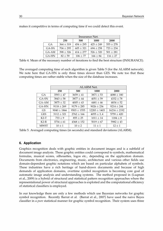
Bayesian Network30
makes it competitive in terms of computing time if we could detect this event.
Insurance Net.250 500 1000 2000
GA 364 ± 319 454 ± 295 425 ± 249 555 ± 278GA-SN 704 ± 295 605 ± 321 694 ± 258 723 ± 234GA-AM 398 ± 326 414 ± 277 526 ± 320 501 ± 281GA-HN 82 ± 59 106 ± 77 166 ± 84 116 ± 27
Table 4. Mean of the necessary number of iterations to find the best structure (INSURANCE).
The averaged computing time of each algorithm is given Table 5 (for the ALARM network).We note here that GA-HN is only three times slower than GES. We note too that thesecomputing times are rather stable when the size of the database increases.
ALARM Net.250 500 1000 2000
GA 3593 ± 47 3659 ± 41 3871 ± 53 4088 ± 180GA-SN 3843 ± 58 3877 ± 44 4051 ± 59 4332 ± 78GA-AM 3875 ± 32 4005 ± 43 4481 ± 46 4834 ± 52GA-HN 9118 ± 269 9179 ± 285 9026 ± 236 9214 ± 244
GS 9040 ± 1866 9503 ± 1555 12283 ± 1403 16216 ± 2192GES 3112 ± 321 2762 ± 166 4055 ± 3, 4 5759 ± 420K2-T 733 ± 9 855 ± 25 1011 ± 14 1184 ± 8K2-R 3734 ± 61 4368 ± 152 5019 ± 67 5982 ± 43
MWST 10 ± 1 10 ± 2 11 ± 1 12 ± 1
Table 5. Averaged computing times (in seconds) and standard deviations (ALARM).
6. Application
Graphics recognition deals with graphic entities in document images and is a subfield ofdocument image analysis. These graphic entities could correspond to symbols, mathematicalformulas, musical scores, silhouettes, logos etc., depending on the application domain.Documents from electronics, engineering, music, architecture and various other fields usedomain-dependent graphic notations which are based on particular alphabets of symbols.These industries have a rich heritage of hand-drawn documents and because of highdemands of application domains, overtime symbol recognition is becoming core goal ofautomatic image analysis and understanding systems. The method proposed in (Luqmanet al., 2009) is a hybrid of structural and statistical pattern recognition approaches where therepresentational power of structural approaches is exploited and the computational efficiencyof statistical classifiers is employed.
In our knowledge there are only a few methods which use Bayesian networks for graphicsymbol recognition. Recently Barrat et al. (Barrat et al., 2007) have used the naive Bayesclassifier in a pure statistical manner for graphic symbol recognition. Their system uses three
shape descriptors: Generic Fourier Descriptor, Zernike descriptor & R-Signature 1D, andapplies dimensionality reduction for extracting the most relevant and discriminating featuresto formulate a feature vector. This reduces the length of their feature vector and eventuallythe number of variables (nodes) in Bayesian network. The naive Bayes classifier is a powerfulBayesian classifier but it assumes a strong independence relationship among attributes giventhe class variable. We believe that the power of Bayesian networks is not fully explored;as instead of using predefined dependency relationships, if we find dependencies betweenall variable pairs from underlying data we can obtain a more powerful Bayesian networkclassifier. This will also help to ignore irrelevant variables and exploit the variables that areinteresting for discriminating symbols in underlying symbol set.
Our method is an original adaptation of Bayesian network learning for the problem ofgraphic symbol recognition. For symbol representation, we use a structural signature. Thesignature is computed from the attributed relational graph (ARG) of symbol and is composedof geometric & topologic characteristics of the structure of symbol. We use (overlapping)fuzzy intervals for computing noise sensitive features in signature. This increases the abilityof our signature to resist against irregularities (Mitra & Pal, 2005) that may be introduced inthe shape of symbol by deformations & degradations. For symbol recognition, we employa Bayesian network. This network is learned from underlying training data by using theGA-HN algorithm. A query symbol is classified by using Bayesian probabilistic inference(on encoded joint probability distribution). We have selected the features in signature verycarefully to best suit them to linear graphic symbols and to restrict their number to minimum;as Bayesian network algorithms are known to perform better for a smaller number of nodes.Our structural signature makes the proposed system robust & independent of applicationdomains and it could be used for all types of 2D linear graphic symbols.
After representing the symbols in learning set by ARG and describing them by structuralsignatures, we proceed to learning of a Bayesian network. The signatures are first dis-cretized. We discretize each feature variable (of signature) separately and independentlyof others. The class labels are chosen intelligently in order to avoid the need of any dis-cretization for them. The discretization of number of nodes and number of arcs achieves acomparison of similarity of symbols (instead of strict comparison of exact feature values).This discretization step also ensures that the features in signature of query symbol will lookfor symbols whose number of nodes and arcs lie in same intervals as that of the query symbol.
The Bayesian network is learned in two steps. First we learn the structure of the network.Despite the training algorithms are evolutionary one, they have provided stable results (fora given dataset multiple invocations always returned identical network structures). Eachfeature in signature becomes a node of network. The goal of structure learning stage is tofind the best network structure from underlying data which contains all possible dependencyrelationships between all variable pairs. The structure of the learned network depicts thedependency relationships between different features in signature. Fig.3 shows one of thelearned structures from our experiments. The second step is learning of parameters ofnetwork; which are conditional probability distributions Pr(nodei|parentsi) associated tonodes of the network and which quantify the dependency relationships between nodes.The network parameters are obtained by maximum likelihood estimation (MLE); which is arobust parameter estimation technique and assigns the most likely parameter values to best

Design of evolutionary methods applied to the learning of Bayesian network structures 31
makes it competitive in terms of computing time if we could detect this event.
Insurance Net.250 500 1000 2000
GA 364 ± 319 454 ± 295 425 ± 249 555 ± 278GA-SN 704 ± 295 605 ± 321 694 ± 258 723 ± 234GA-AM 398 ± 326 414 ± 277 526 ± 320 501 ± 281GA-HN 82 ± 59 106 ± 77 166 ± 84 116 ± 27
Table 4. Mean of the necessary number of iterations to find the best structure (INSURANCE).
The averaged computing time of each algorithm is given Table 5 (for the ALARM network).We note here that GA-HN is only three times slower than GES. We note too that thesecomputing times are rather stable when the size of the database increases.
ALARM Net.250 500 1000 2000
GA 3593 ± 47 3659 ± 41 3871 ± 53 4088 ± 180GA-SN 3843 ± 58 3877 ± 44 4051 ± 59 4332 ± 78GA-AM 3875 ± 32 4005 ± 43 4481 ± 46 4834 ± 52GA-HN 9118 ± 269 9179 ± 285 9026 ± 236 9214 ± 244
GS 9040 ± 1866 9503 ± 1555 12283 ± 1403 16216 ± 2192GES 3112 ± 321 2762 ± 166 4055 ± 3, 4 5759 ± 420K2-T 733 ± 9 855 ± 25 1011 ± 14 1184 ± 8K2-R 3734 ± 61 4368 ± 152 5019 ± 67 5982 ± 43
MWST 10 ± 1 10 ± 2 11 ± 1 12 ± 1
Table 5. Averaged computing times (in seconds) and standard deviations (ALARM).
6. Application
Graphics recognition deals with graphic entities in document images and is a subfield ofdocument image analysis. These graphic entities could correspond to symbols, mathematicalformulas, musical scores, silhouettes, logos etc., depending on the application domain.Documents from electronics, engineering, music, architecture and various other fields usedomain-dependent graphic notations which are based on particular alphabets of symbols.These industries have a rich heritage of hand-drawn documents and because of highdemands of application domains, overtime symbol recognition is becoming core goal ofautomatic image analysis and understanding systems. The method proposed in (Luqmanet al., 2009) is a hybrid of structural and statistical pattern recognition approaches where therepresentational power of structural approaches is exploited and the computational efficiencyof statistical classifiers is employed.
In our knowledge there are only a few methods which use Bayesian networks for graphicsymbol recognition. Recently Barrat et al. (Barrat et al., 2007) have used the naive Bayesclassifier in a pure statistical manner for graphic symbol recognition. Their system uses three
shape descriptors: Generic Fourier Descriptor, Zernike descriptor & R-Signature 1D, andapplies dimensionality reduction for extracting the most relevant and discriminating featuresto formulate a feature vector. This reduces the length of their feature vector and eventuallythe number of variables (nodes) in Bayesian network. The naive Bayes classifier is a powerfulBayesian classifier but it assumes a strong independence relationship among attributes giventhe class variable. We believe that the power of Bayesian networks is not fully explored;as instead of using predefined dependency relationships, if we find dependencies betweenall variable pairs from underlying data we can obtain a more powerful Bayesian networkclassifier. This will also help to ignore irrelevant variables and exploit the variables that areinteresting for discriminating symbols in underlying symbol set.
Our method is an original adaptation of Bayesian network learning for the problem ofgraphic symbol recognition. For symbol representation, we use a structural signature. Thesignature is computed from the attributed relational graph (ARG) of symbol and is composedof geometric & topologic characteristics of the structure of symbol. We use (overlapping)fuzzy intervals for computing noise sensitive features in signature. This increases the abilityof our signature to resist against irregularities (Mitra & Pal, 2005) that may be introduced inthe shape of symbol by deformations & degradations. For symbol recognition, we employa Bayesian network. This network is learned from underlying training data by using theGA-HN algorithm. A query symbol is classified by using Bayesian probabilistic inference(on encoded joint probability distribution). We have selected the features in signature verycarefully to best suit them to linear graphic symbols and to restrict their number to minimum;as Bayesian network algorithms are known to perform better for a smaller number of nodes.Our structural signature makes the proposed system robust & independent of applicationdomains and it could be used for all types of 2D linear graphic symbols.
After representing the symbols in learning set by ARG and describing them by structuralsignatures, we proceed to learning of a Bayesian network. The signatures are first dis-cretized. We discretize each feature variable (of signature) separately and independentlyof others. The class labels are chosen intelligently in order to avoid the need of any dis-cretization for them. The discretization of number of nodes and number of arcs achieves acomparison of similarity of symbols (instead of strict comparison of exact feature values).This discretization step also ensures that the features in signature of query symbol will lookfor symbols whose number of nodes and arcs lie in same intervals as that of the query symbol.
The Bayesian network is learned in two steps. First we learn the structure of the network.Despite the training algorithms are evolutionary one, they have provided stable results (fora given dataset multiple invocations always returned identical network structures). Eachfeature in signature becomes a node of network. The goal of structure learning stage is tofind the best network structure from underlying data which contains all possible dependencyrelationships between all variable pairs. The structure of the learned network depicts thedependency relationships between different features in signature. Fig.3 shows one of thelearned structures from our experiments. The second step is learning of parameters ofnetwork; which are conditional probability distributions Pr(nodei|parentsi) associated tonodes of the network and which quantify the dependency relationships between nodes.The network parameters are obtained by maximum likelihood estimation (MLE); which is arobust parameter estimation technique and assigns the most likely parameter values to best

Bayesian Network32
describe a given distribution of data. We avoid null probabilities by using Dirichlet priorswith MLE. The learned Bayesian network encodes joint probability distribution of the symbolsignatures.
N
B1
C
A1B2B3
C1 C2
C3D2D3
A2A3
A4
A5 D1 A6
Fig. 3. Example of a Bayesian network : C = class, N = number of nodes, A1 = number ofconnections, A2 = number of L-junctions, A3 = number of T-junctions, A4 = number of in-tersections, A5 = number of parallel connections, A6 = number of successive connections, B1(resp. B2 and B3) = number of nodes with low (resp. medium and high) density of connec-tions, C1 (resp. C2 and C3) = number of small-length (resp. medium-length and full-length)primitives, D1 = number of small-angle (resp. medium-angle and full-angle) connections.
The conditional independence property of Bayesian networks helps us to ignore irrelevantfeatures in structural signature for an underlying symbol set. This property states thata node is conditionally independent of its non-descendants given its immediate parents(Charniak, 1991). Conditional independence of a node in Bayesian network is fully ex-ploited during probabilistic inference and thus helps us to ignore irrelevant features foran underlying symbol set while computing posterior probabilities for different symbol classes.
For recognizing a query symbol we use Bayesian probabilistic inference on the encoded jointprobability distribution. This is achieved by using junction tree inference engine which isthe most popular exact inference engine for Bayesian probabilistic inference. The inferenceengine propagates the evidence (signature of query symbol) in network and computes poste-rior probability for each symbol class. Equation 12 gives Bayes rule for our system. It statesthat posterior probability or probability of a symbol class ci given a query signature evidencee is computed from likelihood (probability of e given ci), prior probability of ci and marginallikelihood (prior probability of e). The marginal likelihood Pr(e) is to normalize the posteriorprobability; it ensures that the probabilities fall between 0 and 1.
Pr(ci|e) =Pr(e, ci)
Pr(e)=
Pr(e|ci)× Pr(ci)
Pr(e)(12)
where,{
e = f1, f2, f3, ..., f16Pr(e) = Pr(e, ci) = ∑k
i=1 Pr(e|ci)× Pr(ci)(13)
The posterior probabilities are computed for all k symbol classes and the query symbol is thenassigned to class which maximizes the posterior probability i.e. which has highest posteriorprobability for the given query symbol.
6.1 Symbols with vectorial and binary noiseThe organization of four international symbol recognition contests over last decade (Aksoyet al., 2000; Dosch & Valveny, 2005; Valveny & Dosch, 2003; Valveny et al., 2007), has providedour community an important test bed for evaluation of methods over a standard dataset.These contests were organized to evaluate and test the symbol recognition methods fortheir scalability and robustness against binary degradation and vectorial deformations.The contests were run on pre-segmented linear symbols from architectural and electronicdrawings, as these symbols are representative of a wide range of shapes (Valveny & Dosch,2003). GREC2005 (Dosch & Valveny, 2005) & GREC2007 (Valveny et al., 2007) databases arecomposed of the same set of models, whereas GREC2003 (Valveny & Dosch, 2003) databaseis a subset of GREC2005.
Fig. 4. Model symbols from electronic drawings and from floor plans.
We experimented with synthetically generated 2D symbols of models collected from databaseof GREC2005. In order to get a true picture of the performance of our proposed methodon this database, we have experimented with 20, 50, 75, 100, 125 & 150 symbol classes. Wegenerated our own learning & test sets (based on deformations & degradations of GREC2005)for our experiments. For each class the perfect symbol (the model) along with its 36 rotatedand 12 scaled examples was used for learning; as the features have already been showninvariant to scaling & rotation and because of the fact that generally Bayesian networklearning algorithms perform better on datasets with large number of examples. The systemhas been tested for its scalability on clean symbols (rotated & scaled), various levels ofvectorial deformations and for binary degradations of GREC symbol recognition contest.Each test dataset was composed of 10 query symbols for each class.
Number of classes (models) 20 50 75 100 125 150Clean symbols (rotated & scaled) 100% 100% 100% 100% 100% 99%Hand-drawn deform. Level-1 99% 96% 93% 92% 90% 89%Hand-drawn deform. Level-2 98% 95% 92% 90% 89% 87%Hand-drawn deform. Level-3 95% 77% 73% 70% 69% 67%Binary degrade 98% 96% 93% 92% 89% 89%
Table 6. Results of symbol recognition experiments.
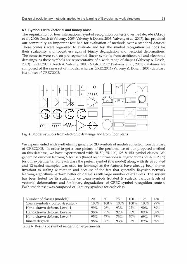
Design of evolutionary methods applied to the learning of Bayesian network structures 33
describe a given distribution of data. We avoid null probabilities by using Dirichlet priorswith MLE. The learned Bayesian network encodes joint probability distribution of the symbolsignatures.
N
B1
C
A1B2B3
C1 C2
C3D2D3
A2A3
A4
A5 D1 A6
Fig. 3. Example of a Bayesian network : C = class, N = number of nodes, A1 = number ofconnections, A2 = number of L-junctions, A3 = number of T-junctions, A4 = number of in-tersections, A5 = number of parallel connections, A6 = number of successive connections, B1(resp. B2 and B3) = number of nodes with low (resp. medium and high) density of connec-tions, C1 (resp. C2 and C3) = number of small-length (resp. medium-length and full-length)primitives, D1 = number of small-angle (resp. medium-angle and full-angle) connections.
The conditional independence property of Bayesian networks helps us to ignore irrelevantfeatures in structural signature for an underlying symbol set. This property states thata node is conditionally independent of its non-descendants given its immediate parents(Charniak, 1991). Conditional independence of a node in Bayesian network is fully ex-ploited during probabilistic inference and thus helps us to ignore irrelevant features foran underlying symbol set while computing posterior probabilities for different symbol classes.
For recognizing a query symbol we use Bayesian probabilistic inference on the encoded jointprobability distribution. This is achieved by using junction tree inference engine which isthe most popular exact inference engine for Bayesian probabilistic inference. The inferenceengine propagates the evidence (signature of query symbol) in network and computes poste-rior probability for each symbol class. Equation 12 gives Bayes rule for our system. It statesthat posterior probability or probability of a symbol class ci given a query signature evidencee is computed from likelihood (probability of e given ci), prior probability of ci and marginallikelihood (prior probability of e). The marginal likelihood Pr(e) is to normalize the posteriorprobability; it ensures that the probabilities fall between 0 and 1.
Pr(ci|e) =Pr(e, ci)
Pr(e)=
Pr(e|ci)× Pr(ci)
Pr(e)(12)
where,{
e = f1, f2, f3, ..., f16Pr(e) = Pr(e, ci) = ∑k
i=1 Pr(e|ci)× Pr(ci)(13)
The posterior probabilities are computed for all k symbol classes and the query symbol is thenassigned to class which maximizes the posterior probability i.e. which has highest posteriorprobability for the given query symbol.
6.1 Symbols with vectorial and binary noiseThe organization of four international symbol recognition contests over last decade (Aksoyet al., 2000; Dosch & Valveny, 2005; Valveny & Dosch, 2003; Valveny et al., 2007), has providedour community an important test bed for evaluation of methods over a standard dataset.These contests were organized to evaluate and test the symbol recognition methods fortheir scalability and robustness against binary degradation and vectorial deformations.The contests were run on pre-segmented linear symbols from architectural and electronicdrawings, as these symbols are representative of a wide range of shapes (Valveny & Dosch,2003). GREC2005 (Dosch & Valveny, 2005) & GREC2007 (Valveny et al., 2007) databases arecomposed of the same set of models, whereas GREC2003 (Valveny & Dosch, 2003) databaseis a subset of GREC2005.
Fig. 4. Model symbols from electronic drawings and from floor plans.
We experimented with synthetically generated 2D symbols of models collected from databaseof GREC2005. In order to get a true picture of the performance of our proposed methodon this database, we have experimented with 20, 50, 75, 100, 125 & 150 symbol classes. Wegenerated our own learning & test sets (based on deformations & degradations of GREC2005)for our experiments. For each class the perfect symbol (the model) along with its 36 rotatedand 12 scaled examples was used for learning; as the features have already been showninvariant to scaling & rotation and because of the fact that generally Bayesian networklearning algorithms perform better on datasets with large number of examples. The systemhas been tested for its scalability on clean symbols (rotated & scaled), various levels ofvectorial deformations and for binary degradations of GREC symbol recognition contest.Each test dataset was composed of 10 query symbols for each class.
Number of classes (models) 20 50 75 100 125 150Clean symbols (rotated & scaled) 100% 100% 100% 100% 100% 99%Hand-drawn deform. Level-1 99% 96% 93% 92% 90% 89%Hand-drawn deform. Level-2 98% 95% 92% 90% 89% 87%Hand-drawn deform. Level-3 95% 77% 73% 70% 69% 67%Binary degrade 98% 96% 93% 92% 89% 89%
Table 6. Results of symbol recognition experiments.
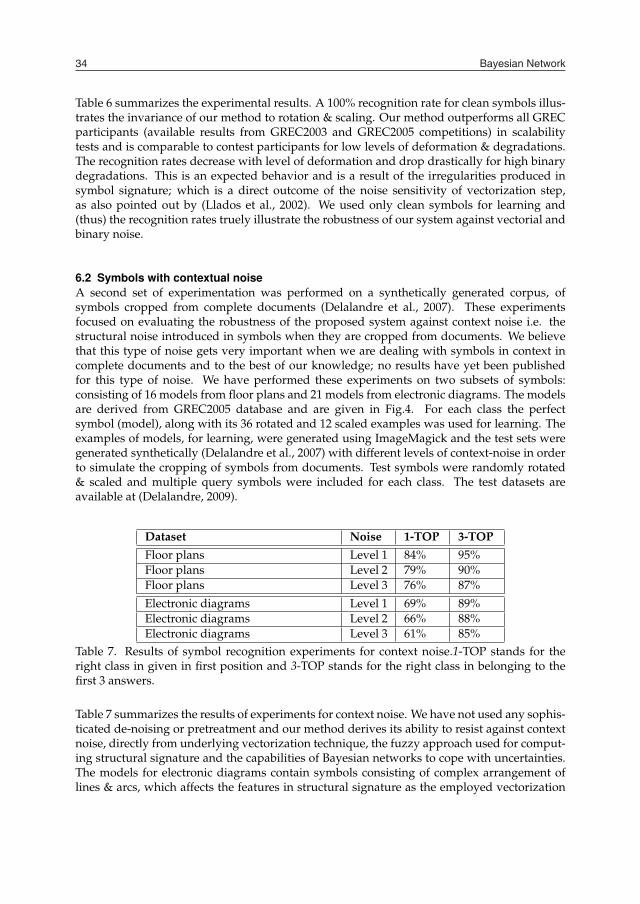
Bayesian Network34
Table 6 summarizes the experimental results. A 100% recognition rate for clean symbols illus-trates the invariance of our method to rotation & scaling. Our method outperforms all GRECparticipants (available results from GREC2003 and GREC2005 competitions) in scalabilitytests and is comparable to contest participants for low levels of deformation & degradations.The recognition rates decrease with level of deformation and drop drastically for high binarydegradations. This is an expected behavior and is a result of the irregularities produced insymbol signature; which is a direct outcome of the noise sensitivity of vectorization step,as also pointed out by (Llados et al., 2002). We used only clean symbols for learning and(thus) the recognition rates truely illustrate the robustness of our system against vectorial andbinary noise.
6.2 Symbols with contextual noiseA second set of experimentation was performed on a synthetically generated corpus, ofsymbols cropped from complete documents (Delalandre et al., 2007). These experimentsfocused on evaluating the robustness of the proposed system against context noise i.e. thestructural noise introduced in symbols when they are cropped from documents. We believethat this type of noise gets very important when we are dealing with symbols in context incomplete documents and to the best of our knowledge; no results have yet been publishedfor this type of noise. We have performed these experiments on two subsets of symbols:consisting of 16 models from floor plans and 21 models from electronic diagrams. The modelsare derived from GREC2005 database and are given in Fig.4. For each class the perfectsymbol (model), along with its 36 rotated and 12 scaled examples was used for learning. Theexamples of models, for learning, were generated using ImageMagick and the test sets weregenerated synthetically (Delalandre et al., 2007) with different levels of context-noise in orderto simulate the cropping of symbols from documents. Test symbols were randomly rotated& scaled and multiple query symbols were included for each class. The test datasets areavailable at (Delalandre, 2009).
Dataset Noise 1-TOP 3-TOPFloor plans Level 1 84% 95%Floor plans Level 2 79% 90%Floor plans Level 3 76% 87%
Electronic diagrams Level 1 69% 89%Electronic diagrams Level 2 66% 88%Electronic diagrams Level 3 61% 85%
Table 7. Results of symbol recognition experiments for context noise.1-TOP stands for theright class in given in first position and 3-TOP stands for the right class in belonging to thefirst 3 answers.
Table 7 summarizes the results of experiments for context noise. We have not used any sophis-ticated de-noising or pretreatment and our method derives its ability to resist against contextnoise, directly from underlying vectorization technique, the fuzzy approach used for comput-ing structural signature and the capabilities of Bayesian networks to cope with uncertainties.The models for electronic diagrams contain symbols consisting of complex arrangement oflines & arcs, which affects the features in structural signature as the employed vectorization
technique is not able to cope with arcs & circles; as is depicted by the recognition rates forthese symbols. But keeping in view the fact that we have used only clean symbols for learn-ing and noisy symbols for testing, we believe that the results show the ability of our signatureto exploit the sufficient structural details of symbols and it could be used to discriminate andrecognize symbols with context noise.
7. Conclusion
We have presented three methods for learning the structure of a Bayesian network. The firstone consists in the control of the probability distribution of mutation in the genetic algorithm.The second one is to incorporate a scheme penalty in the genetic algorithm so that it avoidscertain areas of space research. The third method is to search through several competingpopulations and to allow timely exchange among these populations. We have shown experi-mentally that different algorithms behaved satisfactorily, in particular that they were provingto be successful on large databases. We also examined the behavior of proposed algorithms.Niching strategies are interesting, especially using the spatial one, which focuses quickly onthe best solutions.
8. Acknowledgements
This work was realized using Matlab and two toolboxes dedicated to Bayesian networks ma-nipulation: Bayesian Net Toolbox from K. P. Murphy (Murphy, 2001) and Structure LearningPackage (SLP) from P. Leray & O. François (Francois & Leray, 2004).
9. References
Acid, S. & de Campos, L. M. (2003). Searching for bayesian network structures in the space ofrestricted acyclic partially directed graphs, Journ. of Art. Int. Res. 18: 445–490.
Akaike, H. (1970). Statistical predictor identification, Ann. Inst. Stat. Math. 22(1): 203–217.Aksoy, S., Ye, M., Schauf, M., Song, M., Wang, Y., Haralick, R., Parker, J., Pivovarov, J., Royko,
D., Sun, C. & Farneback, G. (2000). Algorithm performance contest, Proc. of ICPR,pp. 4870–4876.
Allanach, J., Tu, H., Singh, S., Pattipati, K. & Willett, P. (2004). Detecting, tracking and coun-teracting terrorist networks via hidden markov models, Proc. of IEEE Aero. Conf.
Bäck, T. (1993). Optimal mutation rates in genetic search, Proc. of Int. Conf. on Genetic Algo-rithms, Morgan Kaufmann, San Mateo (CA), pp. 2–8.
Barrat, S., Tabbone, S. & Nourrissier, P. (2007). A bayesian classifier for symbol recognition,Proc. of GREC.
Beasley, D., Bull, D. R. & Martin, R. R. (1993). A sequential niche technique for multimodalfunction optimization, Evolutionary Computation 1(2): 101–125.
Beinlich, I. A., Suermondt, H. J., Chavez, R. M. & Cooper, G. F. (1989). The alarm monitoringsystem: A case study with two probabilistic inference techniques for belief networks,Proc. of Eur. Conf. Art. Int. in Med., Springer Verlag, Berlin, pp. 247–256.
Binder, J., Koller, D., Russell, S. J. & Kanazawa, K. (1997). Adaptive probabilistic networkswith hidden variables, Machine Learning 29(2-3): 213–244.
Blanco, R., Inza, I. & Larrañaga, P. (2003). Learning bayesian networks in the space of struc-tures by estimation of distribution algorithms., Int. Jour. of Int. Syst. 18(2): 205–220.
Bouckaert, R. (1994). Properties of bayesian belief network learning algorithms, Proc. of Un-certainty in Artificial Intelligence, Morgan Kaufmann, San Francisco, CA, pp. 102–110.

Design of evolutionary methods applied to the learning of Bayesian network structures 35
Table 6 summarizes the experimental results. A 100% recognition rate for clean symbols illus-trates the invariance of our method to rotation & scaling. Our method outperforms all GRECparticipants (available results from GREC2003 and GREC2005 competitions) in scalabilitytests and is comparable to contest participants for low levels of deformation & degradations.The recognition rates decrease with level of deformation and drop drastically for high binarydegradations. This is an expected behavior and is a result of the irregularities produced insymbol signature; which is a direct outcome of the noise sensitivity of vectorization step,as also pointed out by (Llados et al., 2002). We used only clean symbols for learning and(thus) the recognition rates truely illustrate the robustness of our system against vectorial andbinary noise.
6.2 Symbols with contextual noiseA second set of experimentation was performed on a synthetically generated corpus, ofsymbols cropped from complete documents (Delalandre et al., 2007). These experimentsfocused on evaluating the robustness of the proposed system against context noise i.e. thestructural noise introduced in symbols when they are cropped from documents. We believethat this type of noise gets very important when we are dealing with symbols in context incomplete documents and to the best of our knowledge; no results have yet been publishedfor this type of noise. We have performed these experiments on two subsets of symbols:consisting of 16 models from floor plans and 21 models from electronic diagrams. The modelsare derived from GREC2005 database and are given in Fig.4. For each class the perfectsymbol (model), along with its 36 rotated and 12 scaled examples was used for learning. Theexamples of models, for learning, were generated using ImageMagick and the test sets weregenerated synthetically (Delalandre et al., 2007) with different levels of context-noise in orderto simulate the cropping of symbols from documents. Test symbols were randomly rotated& scaled and multiple query symbols were included for each class. The test datasets areavailable at (Delalandre, 2009).
Dataset Noise 1-TOP 3-TOPFloor plans Level 1 84% 95%Floor plans Level 2 79% 90%Floor plans Level 3 76% 87%
Electronic diagrams Level 1 69% 89%Electronic diagrams Level 2 66% 88%Electronic diagrams Level 3 61% 85%
Table 7. Results of symbol recognition experiments for context noise.1-TOP stands for theright class in given in first position and 3-TOP stands for the right class in belonging to thefirst 3 answers.
Table 7 summarizes the results of experiments for context noise. We have not used any sophis-ticated de-noising or pretreatment and our method derives its ability to resist against contextnoise, directly from underlying vectorization technique, the fuzzy approach used for comput-ing structural signature and the capabilities of Bayesian networks to cope with uncertainties.The models for electronic diagrams contain symbols consisting of complex arrangement oflines & arcs, which affects the features in structural signature as the employed vectorization
technique is not able to cope with arcs & circles; as is depicted by the recognition rates forthese symbols. But keeping in view the fact that we have used only clean symbols for learn-ing and noisy symbols for testing, we believe that the results show the ability of our signatureto exploit the sufficient structural details of symbols and it could be used to discriminate andrecognize symbols with context noise.
7. Conclusion
We have presented three methods for learning the structure of a Bayesian network. The firstone consists in the control of the probability distribution of mutation in the genetic algorithm.The second one is to incorporate a scheme penalty in the genetic algorithm so that it avoidscertain areas of space research. The third method is to search through several competingpopulations and to allow timely exchange among these populations. We have shown experi-mentally that different algorithms behaved satisfactorily, in particular that they were provingto be successful on large databases. We also examined the behavior of proposed algorithms.Niching strategies are interesting, especially using the spatial one, which focuses quickly onthe best solutions.
8. Acknowledgements
This work was realized using Matlab and two toolboxes dedicated to Bayesian networks ma-nipulation: Bayesian Net Toolbox from K. P. Murphy (Murphy, 2001) and Structure LearningPackage (SLP) from P. Leray & O. François (Francois & Leray, 2004).
9. References
Acid, S. & de Campos, L. M. (2003). Searching for bayesian network structures in the space ofrestricted acyclic partially directed graphs, Journ. of Art. Int. Res. 18: 445–490.
Akaike, H. (1970). Statistical predictor identification, Ann. Inst. Stat. Math. 22(1): 203–217.Aksoy, S., Ye, M., Schauf, M., Song, M., Wang, Y., Haralick, R., Parker, J., Pivovarov, J., Royko,
D., Sun, C. & Farneback, G. (2000). Algorithm performance contest, Proc. of ICPR,pp. 4870–4876.
Allanach, J., Tu, H., Singh, S., Pattipati, K. & Willett, P. (2004). Detecting, tracking and coun-teracting terrorist networks via hidden markov models, Proc. of IEEE Aero. Conf.
Bäck, T. (1993). Optimal mutation rates in genetic search, Proc. of Int. Conf. on Genetic Algo-rithms, Morgan Kaufmann, San Mateo (CA), pp. 2–8.
Barrat, S., Tabbone, S. & Nourrissier, P. (2007). A bayesian classifier for symbol recognition,Proc. of GREC.
Beasley, D., Bull, D. R. & Martin, R. R. (1993). A sequential niche technique for multimodalfunction optimization, Evolutionary Computation 1(2): 101–125.
Beinlich, I. A., Suermondt, H. J., Chavez, R. M. & Cooper, G. F. (1989). The alarm monitoringsystem: A case study with two probabilistic inference techniques for belief networks,Proc. of Eur. Conf. Art. Int. in Med., Springer Verlag, Berlin, pp. 247–256.
Binder, J., Koller, D., Russell, S. J. & Kanazawa, K. (1997). Adaptive probabilistic networkswith hidden variables, Machine Learning 29(2-3): 213–244.
Blanco, R., Inza, I. & Larrañaga, P. (2003). Learning bayesian networks in the space of struc-tures by estimation of distribution algorithms., Int. Jour. of Int. Syst. 18(2): 205–220.
Bouckaert, R. (1994). Properties of bayesian belief network learning algorithms, Proc. of Un-certainty in Artificial Intelligence, Morgan Kaufmann, San Francisco, CA, pp. 102–110.
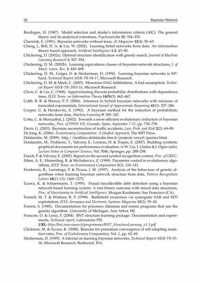
Bayesian Network36
Bozdogan, H. (1987). Model selection and akaike’s information criteria (AIC): The generaltheory and its analytical extentions, Psychometrika 52: 354–370.
Charniak, E. (1991). Bayesian networks without tears, AI Magazine 12(4): 50–63.Cheng, J., Bell, D. A. & Liu, W. (2002). Learning belief networks from data: An information
theory based approach, Artificial Intelligence 1-2: 43–90.Chickering, D. (2002a). Optimal structure identification with greedy search, Journal of Machine
Learning Research 3: 507–554.Chickering, D. M. (2002b). Learning equivalence classes of bayesian-network structures, J. of
Mach. Learn. Res. 2: 445–498.Chickering, D. M., Geiger, D. & Heckerman, D. (1994). Learning bayesian networks is NP-
hard, Technical Report MSR-TR-94-17, Microsoft Research.Chickering, D. M. & Meek, C. (2003). Monotone DAG faithfulness: A bad assumption, Techni-
cal Report MSR-TR-2003-16, Microsoft Research.Chow, C. & Liu, C. (1968). Approximating discrete probability distributions with dependence
trees, IEEE Trans. on Information Theory 14(3)(3): 462–467.Cobb, B. R. & Shenoy, P. P. (2006). Inference in hybrid bayesian networks with mixtures of
truncated exponentials, International Jounal of Approximate Reasoning 41(3): 257–286.Cooper, G. & Herskovits, E. (1992). A bayesian method for the induction of probabilistic
networks from data, Machine Learning 9: 309–347.Cotta, C. & Muruzábal, J. (2002). Towards a more efficient evolutionary induction of bayesian
networks., Proc. of PPSN VII, Granada, Spain, September 7-11, pp. 730–739.Davis, G. (2003). Bayesian reconstruction of traffic accidents, Law, Prob. and Risk 2(2): 69–89.De Jong, K. (2006). Evolutionary Computation: A Unified Approach, The MIT Press.Delalandre, M. (2009). http://mathieu.delalandre.free.fr/projects/sesyd/queries.html.Delalandre, M., Pridmore, T., Valveny, E., Locteau, H. & Trupin, E. (2007). Building synthetic
graphical documents for performance evaluation, in W. Liu, J. Llados & J. Ogier (eds),Lecture Notes in Computer Science, Vol. 5046, Springer, pp. 288–298.
Dosch, P. & Valveny, E. (2005). Report on the second symbol recognition contest, Proc. of GREC.Eiben, A. E., Hinterding, R. & Michalewicz, Z. (1999). Parameter control in evolutionary algo-
rithms, IEEE Trans. on Evolutionary Computation 3(2): 124–141.Etxeberria, R., Larrañaga, P. & Picaza, J. M. (1997). Analysis of the behaviour of genetic al-
gorithms when learning bayesian network structure from data, Pattern RecognitionLetters 18(11-13): 1269–1273.
Ezawa, K. & Schuermann, T. (1995). Fraud/uncollectible debt detection using a bayesiannetwork based learning system: A rare binary outcome with mixed data structures,Proc. of Uncertainty in Artificial Intelligence, Morgan Kaufmann, San Francisco (CA).
Fennell, M. T. & Wishner, R. P. (1998). Battlefield awareness via synergistic SAR and MTIexploitation, IEEE Aerospace and Electronic Systems Magazine 13(2): 39–43.
Forrest, S. (1985). Documentation for prisoners dilemma and norms programs that use thegenetic algorithm. University of Michigan, Ann Arbor, MI.
Francois, O. & Leray, P. (2004). BNT structure learning package: Documentation and experi-ments, Technical report, Laboratoire PSI.URL: http://bnt.insa-rouen.fr/programmes/BNT_StructureLearning_v1.3.pdf
Glickman, M. & Sycara, K. (2000). Reasons for premature convergence of self-adapting muta-tion rates, Proc. of Evolutionary Computation, Vol. 1, pp. 62–69.
Heckerman, D. (1995). A tutorial on learning bayesian networks, Technical Report MSR-TR-95-06, Microsoft Research, Redmond, WA.
Henrion, M. (1988). Propagation of uncertainty by probabilistic logic sampling in bayes net-works, Proc. of Uncertainty in Artificial Intelligence, Vol. 2, Morgan Kaufmann, SanFrancisco (CA), pp. 149–164.
Holland, J. H. (1992). Adaptation in natural and artificial systems, MIT Press.Horvitz, E., Breese, J., Heckerman, D., Hovel, D. & Rommelse, K. (1998). The lumiere project:
Bayesian user modeling for inferring the goals and needs of software users, Proc. ofUncertainty in Artificial Intelligence, Morgan Kaufmann, San Francisco (CA).
Hurvich, C. M. & Tsai, C.-L. (1989). Regression and time series model selection in small sam-ples, Biometrika 76(2): 297–307.
Jaronski, W., Bloemer, J., Vanhoof, K. & Wets, G. (2001). Use of bayesian belief networks tohelp understand online audience, Proc. of the ECML/PKDD, Freiburg, Germany.
Kayaalp, M. & Cooper, G. F. (2002). A bayesian network scoring metric that is based on glob-ally uniform parameter priors, Proc. of Uncertainty in Artificial Intelligence, MorganKaufmann, San Francisco, CA, pp. 251–258.
Krause, P. J. (1999). Learning probabilistic networks, Know. Eng. Rev. Arc. 13(4): 321–351.Kreinovich, V., Quintana, C. & Fuentes, O. (1993). Genetic algorithms: What fitness scaling is
optimal?, Cybernetics and Systems 24(1): 9–26.Lacey, G. & MacNamara, S. (2000). Context-aware shared control of a robot mobility aid for
the elderly blind, Int. Journal of Robotic Research 19(11): 1054–1065.Larrañaga, P., Poza, M., Yurramendi, Y., Murga, R. & Kuijpers, C. (1996). Structure learn-
ing of bayesian networks by genetic algorithms: A performance analysis of controlparameters., IEEE Trans. on PAMI 18(9): 912–926.
Lauritzen, S. L. (1995). The EM algorithm for graphical association models with missing data.,Computational Statistics & Data Analysis 19(2): 191–201.
Lauritzen, S. L. & Wermuth, N. (1989). Graphical models for associations between variables,some of which are qualitative and some quantitative, Annals of Statistics 17(1): 31–57.
Lerner, U., Segal, E. & Koller, D. (2001). Exact inference in networks with discrete children ofcontinuous parents, Proc. of UAI, Morgan Kaufmann, San Francisco, CA, pp. 319–332.
Llados, J., Valveny, E., Sanchez, G. & Marti, E. (2002). Symbol recognition: Current advancesand perspectives, Lecture Notes in Computer Science, Vol. 2390, Springer, pp. 104–128.
Luqman, M. M., Brouard, T. & Ramel, J.-Y. (2009). Graphic symbol recognition using graphbased signature and bayesian network classifier, International Conference on DocumentAnalysis and Recognition, IEEE Comp. Soc., Los Alamitos, CA, USA, pp. 1325–1329.
Madigan, D. & York, J. (1995). Bayesian graphical models for discrete data, Int. Stat. Rev.63(2): 215–232.
Mahfoud, S. W. (1995). Niching methods for genetic algorithms, PhD thesis, University of Illinoisat Urbana-Champaign, Urbana, IL, USA. IlliGAL Report 95001.
Mitra, S. & Pal, S. (2005). Fuzzy sets in pattern recognition and machine intelligence, FuzzySets and Systems 156(3): 381–386.
Mühlenbein, H. & PaaB, G. (1996). From recombination of genes to the estimation of distribu-tions, Proc. of PPSN, Vol. 1411, pp. 178–187.
Murphy, K. (2001). The bayes net toolbox for matlab, Comp. Sci. and Stat. 33: 331–350.Muruzábal, J. & Cotta, C. (2004). A primer on the evolution of equivalence classes of bayesian-
network structures, Proc. of PPSN, Birmingham, UK, pp. 612–621.Muruzábal, J. & Cotta, C. (2007). A study on the evolution of bayesian network graph struc-
tures, Studies in Fuzziness and Soft Computing 213: 193–214,.

Design of evolutionary methods applied to the learning of Bayesian network structures 37
Bozdogan, H. (1987). Model selection and akaike’s information criteria (AIC): The generaltheory and its analytical extentions, Psychometrika 52: 354–370.
Charniak, E. (1991). Bayesian networks without tears, AI Magazine 12(4): 50–63.Cheng, J., Bell, D. A. & Liu, W. (2002). Learning belief networks from data: An information
theory based approach, Artificial Intelligence 1-2: 43–90.Chickering, D. (2002a). Optimal structure identification with greedy search, Journal of Machine
Learning Research 3: 507–554.Chickering, D. M. (2002b). Learning equivalence classes of bayesian-network structures, J. of
Mach. Learn. Res. 2: 445–498.Chickering, D. M., Geiger, D. & Heckerman, D. (1994). Learning bayesian networks is NP-
hard, Technical Report MSR-TR-94-17, Microsoft Research.Chickering, D. M. & Meek, C. (2003). Monotone DAG faithfulness: A bad assumption, Techni-
cal Report MSR-TR-2003-16, Microsoft Research.Chow, C. & Liu, C. (1968). Approximating discrete probability distributions with dependence
trees, IEEE Trans. on Information Theory 14(3)(3): 462–467.Cobb, B. R. & Shenoy, P. P. (2006). Inference in hybrid bayesian networks with mixtures of
truncated exponentials, International Jounal of Approximate Reasoning 41(3): 257–286.Cooper, G. & Herskovits, E. (1992). A bayesian method for the induction of probabilistic
networks from data, Machine Learning 9: 309–347.Cotta, C. & Muruzábal, J. (2002). Towards a more efficient evolutionary induction of bayesian
networks., Proc. of PPSN VII, Granada, Spain, September 7-11, pp. 730–739.Davis, G. (2003). Bayesian reconstruction of traffic accidents, Law, Prob. and Risk 2(2): 69–89.De Jong, K. (2006). Evolutionary Computation: A Unified Approach, The MIT Press.Delalandre, M. (2009). http://mathieu.delalandre.free.fr/projects/sesyd/queries.html.Delalandre, M., Pridmore, T., Valveny, E., Locteau, H. & Trupin, E. (2007). Building synthetic
graphical documents for performance evaluation, in W. Liu, J. Llados & J. Ogier (eds),Lecture Notes in Computer Science, Vol. 5046, Springer, pp. 288–298.
Dosch, P. & Valveny, E. (2005). Report on the second symbol recognition contest, Proc. of GREC.Eiben, A. E., Hinterding, R. & Michalewicz, Z. (1999). Parameter control in evolutionary algo-
rithms, IEEE Trans. on Evolutionary Computation 3(2): 124–141.Etxeberria, R., Larrañaga, P. & Picaza, J. M. (1997). Analysis of the behaviour of genetic al-
gorithms when learning bayesian network structure from data, Pattern RecognitionLetters 18(11-13): 1269–1273.
Ezawa, K. & Schuermann, T. (1995). Fraud/uncollectible debt detection using a bayesiannetwork based learning system: A rare binary outcome with mixed data structures,Proc. of Uncertainty in Artificial Intelligence, Morgan Kaufmann, San Francisco (CA).
Fennell, M. T. & Wishner, R. P. (1998). Battlefield awareness via synergistic SAR and MTIexploitation, IEEE Aerospace and Electronic Systems Magazine 13(2): 39–43.
Forrest, S. (1985). Documentation for prisoners dilemma and norms programs that use thegenetic algorithm. University of Michigan, Ann Arbor, MI.
Francois, O. & Leray, P. (2004). BNT structure learning package: Documentation and experi-ments, Technical report, Laboratoire PSI.URL: http://bnt.insa-rouen.fr/programmes/BNT_StructureLearning_v1.3.pdf
Glickman, M. & Sycara, K. (2000). Reasons for premature convergence of self-adapting muta-tion rates, Proc. of Evolutionary Computation, Vol. 1, pp. 62–69.
Heckerman, D. (1995). A tutorial on learning bayesian networks, Technical Report MSR-TR-95-06, Microsoft Research, Redmond, WA.
Henrion, M. (1988). Propagation of uncertainty by probabilistic logic sampling in bayes net-works, Proc. of Uncertainty in Artificial Intelligence, Vol. 2, Morgan Kaufmann, SanFrancisco (CA), pp. 149–164.
Holland, J. H. (1992). Adaptation in natural and artificial systems, MIT Press.Horvitz, E., Breese, J., Heckerman, D., Hovel, D. & Rommelse, K. (1998). The lumiere project:
Bayesian user modeling for inferring the goals and needs of software users, Proc. ofUncertainty in Artificial Intelligence, Morgan Kaufmann, San Francisco (CA).
Hurvich, C. M. & Tsai, C.-L. (1989). Regression and time series model selection in small sam-ples, Biometrika 76(2): 297–307.
Jaronski, W., Bloemer, J., Vanhoof, K. & Wets, G. (2001). Use of bayesian belief networks tohelp understand online audience, Proc. of the ECML/PKDD, Freiburg, Germany.
Kayaalp, M. & Cooper, G. F. (2002). A bayesian network scoring metric that is based on glob-ally uniform parameter priors, Proc. of Uncertainty in Artificial Intelligence, MorganKaufmann, San Francisco, CA, pp. 251–258.
Krause, P. J. (1999). Learning probabilistic networks, Know. Eng. Rev. Arc. 13(4): 321–351.Kreinovich, V., Quintana, C. & Fuentes, O. (1993). Genetic algorithms: What fitness scaling is
optimal?, Cybernetics and Systems 24(1): 9–26.Lacey, G. & MacNamara, S. (2000). Context-aware shared control of a robot mobility aid for
the elderly blind, Int. Journal of Robotic Research 19(11): 1054–1065.Larrañaga, P., Poza, M., Yurramendi, Y., Murga, R. & Kuijpers, C. (1996). Structure learn-
ing of bayesian networks by genetic algorithms: A performance analysis of controlparameters., IEEE Trans. on PAMI 18(9): 912–926.
Lauritzen, S. L. (1995). The EM algorithm for graphical association models with missing data.,Computational Statistics & Data Analysis 19(2): 191–201.
Lauritzen, S. L. & Wermuth, N. (1989). Graphical models for associations between variables,some of which are qualitative and some quantitative, Annals of Statistics 17(1): 31–57.
Lerner, U., Segal, E. & Koller, D. (2001). Exact inference in networks with discrete children ofcontinuous parents, Proc. of UAI, Morgan Kaufmann, San Francisco, CA, pp. 319–332.
Llados, J., Valveny, E., Sanchez, G. & Marti, E. (2002). Symbol recognition: Current advancesand perspectives, Lecture Notes in Computer Science, Vol. 2390, Springer, pp. 104–128.
Luqman, M. M., Brouard, T. & Ramel, J.-Y. (2009). Graphic symbol recognition using graphbased signature and bayesian network classifier, International Conference on DocumentAnalysis and Recognition, IEEE Comp. Soc., Los Alamitos, CA, USA, pp. 1325–1329.
Madigan, D. & York, J. (1995). Bayesian graphical models for discrete data, Int. Stat. Rev.63(2): 215–232.
Mahfoud, S. W. (1995). Niching methods for genetic algorithms, PhD thesis, University of Illinoisat Urbana-Champaign, Urbana, IL, USA. IlliGAL Report 95001.
Mitra, S. & Pal, S. (2005). Fuzzy sets in pattern recognition and machine intelligence, FuzzySets and Systems 156(3): 381–386.
Mühlenbein, H. & PaaB, G. (1996). From recombination of genes to the estimation of distribu-tions, Proc. of PPSN, Vol. 1411, pp. 178–187.
Murphy, K. (2001). The bayes net toolbox for matlab, Comp. Sci. and Stat. 33: 331–350.Muruzábal, J. & Cotta, C. (2004). A primer on the evolution of equivalence classes of bayesian-
network structures, Proc. of PPSN, Birmingham, UK, pp. 612–621.Muruzábal, J. & Cotta, C. (2007). A study on the evolution of bayesian network graph struc-
tures, Studies in Fuzziness and Soft Computing 213: 193–214,.
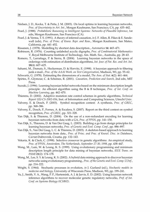
Bayesian Network38
Nielsen, J. D., Kocka, T. & Peña, J. M. (2003). On local optima in learning bayesian networks,Proc. of Uncertainty in Art. Int., Morgan Kaufmann, San Francisco, CA, pp. 435–442.
Pearl, J. (1988). Probabilistic Reasoning in Intelligent Systems: Networks of Plausible Inference, 1stedn, Morgan Kaufmann, San Francisco (CA).
Pearl, J. & Verma, T. S. (1991). A theory of inferred causation, in J. F. Allen, R. Fikes & E. Sande-wall (eds), Proc. of Princ. of Know. Repr. and Reas., Morgan Kaufmann, San Mateo,California, pp. 441–452.
Rissanen, J. (1978). Modelling by shortest data description., Automatica 14: 465–471.Robinson, R. (1976). Counting unlabeled acyclic digraphs, Proc. of Combinatorial Mathematics
V, Royal Melbourne Institute of Technology, Am. Math. Soc., Australia, pp. 28–43.Romero, T., Larrañaga, P. & Sierra, B. (2004). Learning bayesian networks in the space of
orderings with estimation of distribution algorithms, Int. Jour. of Pat. Rec. and Art. Int.18(4): 607–625.
Sahami, M., Dumais, S., Heckerman, D. & Horvitz, E. (1998). A bayesian approach to filteringjunk e-mail., Proc. of the AAAI Work. on Text Categorization, Madison, WI, pp. 55–62.
Schwartz, G. (1978). Estimating the dimensions of a model, The Ann. of Stat. 6(2): 461–464.Spirtes, P., Glymour, C. & Scheines, R. (2001). Causation, Prediction and Search, 2nd edn, MIT
Press.Suzuki, J. (1996). Learning bayesian belief networks based on the minimum description length
principle: An efficient algorithm using the B & B technique, Proc. of Int. Conf. onMachine Learning, pp. 462–470.
Thierens, D. (2002). Adaptive mutation rate control schemes in genetic algorithms, TechnicalReport UU-CS-2002-056, Inst. of Information and Computing Sciences, Utrecht Univ.
Valveny, E. & Dosch, P. (2003). Symbol recognition contest: A synthesis, Proc. of GREC,pp. 368–386.
Valveny, E., Dosch, P., Fornes, A. & Escalera, S. (2007). Report on the third contest on symbolrecognition, Proc. of GREC, pp. 321–328.
Van Dijk, S. & Thierens, D. (2004). On the use of a non-redundant encoding for learningbayesian networks from data with a GA, Proc. of PPSN, pp. 141–150.
Van Dijk, S., Thierens, D. & Van Der Gaag, L. (2003). Building a ga from design principles forlearning bayesian networks, Proc. of Genetic and Evol. Comp. Conf., pp. 886–897.
Van Dijk, S., Van Der Gaag, L. C. & Thierens, D. (2003). A skeleton-based approach to learningbayesian networks from data., Proc. of Princ. and Prac. of Knowl. Disc. in Databases,Cavtat-Dubrovnik, Croatia, pp. 132–143.
Vekaria, K. & Clack, C. (1998). Selective crossover in genetic algorithms: An empirical study,Proc. of PPSN, Amsterdam, The Netherlands, September 27-30, 1998, pp. 438–447.
Wong, M., Lam, W. & Leung, K. S. (1999). Using evolutionary programming and minimumdescription length principle for data mining of bayesian networks, IEEE Trans. onPAMI 21(2): 174–178.
Wong, M., Lee, S. Y. & Leung, K. S. (2002). A hybrid data mining approach to discover bayesiannetworks using evolutionary programming., Proc. of the Genetic and Evol. Comp. COnf.,pp. 214–222.
Wright, S. (1964). Stochastic processes in evolution, in J. Gurland (ed.), Stochastic models inmedecine and biology, University of Wisconsin Press, Madison, WI, pp. 199–241.
Yu, J., Smith, V. A., Wang, P. P., Hartemink, A. J. & Jarvis, E. D. (2002). Using bayesian networkinference algorithms to recover molecular genetic regulatory networks, Prof. of Int.Conf. on Systems Biology (ICSB02).
Related Documents