Design of a SystemView Simulation of a Stepped Frequency Continuous Wave Ground Penetrating Radar Prepared By Andile Mngadi Final year Electrical Engineering Student University of Cape Town This thesis is submitted to the Department of Electrical Engineering, University of Cape Town, in partial fulfilment of the requirements for the degree of Bachelor of Science in Engineering. Cape Town, October 2004 25th October 2004 Document No: rrsg:00

Welcome message from author
This document is posted to help you gain knowledge. Please leave a comment to let me know what you think about it! Share it to your friends and learn new things together.
Transcript

Design of a SystemView Simulation of a Stepped
Frequency Continuous Wave Ground Penetrating
Radar
Prepared By
Andile Mngadi
Final year Electrical Engineering Student
University of Cape Town
This thesis is submitted to the Department of Electrical Engineering,
University of Cape Town, in partial fulfilment of the requirements
for the degree of Bachelor of Science in Engineering.
Cape Town, October 2004
25th October 2004
Document No: rrsg:00

UCT Radar RemoteSensing Group
Department ofElectrical Engineering
Approval
Name Designation Affiliation Date Signature
SubmittedbyReviewedbyAcceptedbyApprovedbyApprovedbyApprovedby
Document History
Revision Date of Issue RRSG Number Comments
A25th October
2004rrsg:00
Document Software
Package Version Filename
Text Processor LYX 1.3.4
Document No. rrsg:00Document Rev. A
25th October 2004Page: 1 of 90

UCT Radar RemoteSensing Group
Department ofElectrical Engineering
Company Details
Name Radar Remote Sensing Group, University of Cape Town
Physical AddressDepartment of Electrical Engineering, Robert Menzies Room609, Universityof Cape Town, Upper Campus, Rondebosch
Postal AddressDepartment of Electrical Engineering, Robert Menzies Room609, Universityof Cape Town, Private Bag, Rondebosch 7701, South Africa
Telephone +27 (0)21 650 2799Fax +27 (0)21 650 3465Email [email protected]
Document No. rrsg:00Document Rev. A
25th October 2004Page: 2 of 90

UCT Radar RemoteSensing Group
Department ofElectrical Engineering
Declaration
I declare that this thesis is my own, unaided work. It is submitted for the degree of Bachelor of
Science in Engineering at the University of Cape Town. It hasnot been submitted before for any
degree or examination in any other university.
Signature of Author....................................
Department of Electrical Engineering,
Cape Town , October 2004
Document No. rrsg:00Document Rev. A
25th October 2004Page: 3 of 90

UCT Radar RemoteSensing Group
Department ofElectrical Engineering
Acknowledgements
I would like to thank my supervisor, Professor Michael Inggs, for his continual support and guidance
throughout the project period. Without his assistance, completion of this project would not have been
possible.
For financially assistance, I am grateful to Denel Pty (Ltd) for their financial assistance throughout
these years.
Thanks to Busisiwe Paliso for keeping me sane, and her support and patience. Many thanks for always
lending a helping hand and keeping me up to date.
To Georgie Goerge, I am thankful for the trouble he went through helping me with simulating the
stepped frequency waveform.
Thanks to Richard Lord, and Andrew Wilkinson for all their support and patience.
Finally I wish to thank the members of the Radar and Remote Sensing Group at University of Cape
Town for their support whenever possible.
To my family.
Document No. rrsg:00Document Rev. A
25th October 2004Page: 4 of 90
UCT Radar RemoteSensing Group
Department ofElectrical Engineering
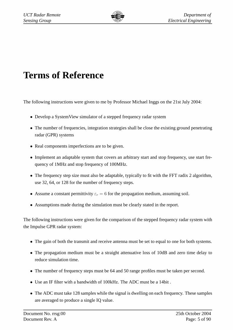
Terms of Reference
The following instructions were given to me by Professor Michael Inggs on the 21st July 2004:
• Develop a SystemView simulator of a stepped frequency radarsystem
• The number of frequencies, integration strategies shall beclose the existing ground penetrating
radar (GPR) systems
• Real components imperfections are to be given.
• Implement an adaptable system that covers an arbitrary start and stop frequency, use start fre-
quency of 1MHz and stop frequency of 100MHz.
• The frequency step size must also be adaptable, typically tofit with the FFT radix 2 algorithm,
use 32, 64, or 128 for the number of frequency steps.
• Assume a constant permittivityεr = 6 for the propagation medium, assuming soil.
• Assumptions made during the simulation must be clearly stated in the report.
The following instructions were given for the comparison ofthe stepped frequency radar system with
the Impulse GPR radar system:
• The gain of both the transmit and receive antenna must be set to equal to one for both systems.
• The propagation medium must be a straight attenuative loss of 10dB and zero time delay to
reduce simulation time.
• The number of frequency steps must be 64 and 50 range profiles must be taken per second.
• Use an IF filter with a bandwidth of 100kHz. The ADC must be a 14bit .
• The ADC must take 128 samples while the signal is dwelling on each frequency. These samples
are averaged to produce a single IQ value.
Document No. rrsg:00Document Rev. A
25th October 2004Page: 5 of 90

UCT Radar RemoteSensing Group
Department ofElectrical Engineering
• The transmit signal power is 10 dBm and the receiver noise figure is 5dB.
The working simulation scripts, test results and the final report are to be submitted on the 19th October
2004.
Document No. rrsg:00Document Rev. A
25th October 2004Page: 6 of 90

UCT Radar RemoteSensing Group
Department ofElectrical Engineering
Synopsis
Research into stepped frequency continuous wave ground penetrating radar (SFCW GPR) has been
carried out since 1990 at UCT. However, this is the first thesis that discusses the simulation of SFCW
GPR using SystemView. SystemView is a time domain system simulator environment for the design
and analysis of engineering, mathematical and scientific systems. Frequency domain analysis of the
signals in SystemView analysis window is also possible.
A SFCW GPR system was simulated in SystemView. Various transmitter configuration were dis-
cussed and the variable parameter configuration was found most suitable and therefore was used for
the simulation. The variable parameter configuration was found most suitable because of its easily
adaptable characteristics. When the variable parameter configuration was used, it was found that
transmitter frequency can be made to cover any arbitrary frequency range, by a simple mouse click.
Also the frequency stepsize and the number of frequency steps were automated when the increment
value was changed, in this configuration. For the simulation, the transmitter covered the 1-100 MHz
frequency band with the transmitter power of 10 mW.
The propagation medium, assumed soil with a constant relative permittivity, was simulated from a
simple attenuator. For a constant relative permittivity, it was found that there is a linear relationship
between the attenuation and frequency. Therefore, the realground characteristics were simulated
based on the attenuation versus frequency relationship. A heterodyne receiver architecture for the
1-100 MHz signal was simulated, to mix the signal to an IF of 1 MHz and demodulate the signal.
Digitisation was performed by a 14 bit quantiser with a 2 V voltage span. The mean noise value
was found important for signal averaging in post processing. Signal processing was not satisfactory,
even though the performance was better than the Impulse GPR system. Zero-padding the range
profile in signal processing improved the high range resolution profile. Stacking was found difficult
in SystemView for the SFCW GPR, the machine ran out of memory when stacking was attempted.
Therefore the alternative was found to be Matlab. This was left out for future work.
The system performance was tested by comparing the SFCW GPR to the Impulse GPR. In terms of
the dynamic range, SNR, and transmit power, the SFCW performance was found better. Advanced
signal processing methods were recommended for the SFCW to further shows its capabilities over the
Impulse GPR. Other recommendations include medium and antenna future work.
Document No. rrsg:00Document Rev. A
25th October 2004Page: 7 of 90

UCT Radar RemoteSensing Group
Department ofElectrical Engineering
List of Symbols
A Amplitude [m]
B Bandwidth [Hz]
Btot Total radar bandwidth [Hz]
c Speed of light [m/s]
F Noise figure [dB]
f Frequency [Hz]
fad A/D sampling frequency [Hz]
fb Beat frequency [Hz]
fc Radar centre transmit frequency [Hz]
fL Lower frequency [Hz]
f0 Start frequency
fs Frequency shift
fU Upper frequency [Hz]
∆f Frequency step size [Hz]
Ga Antenna gain
Gt Transmitter antenna gain
Gr Receiver antenna gain
Hi Range profile transfer function
i A positive integer
n Number of frequency steps
N Number of pulses or signals
N0 Output noise power [dBm]
Pave Average transmitted power [W]
Ppeak Peak transmitted power [W]
P1 1 dB compression point [dB]
P3 Third-order intercept point [dBm]
R Range [m]
Rmax Maximum range [m]
Runam Maximum unambiguous range [m]
Document No. rrsg:00Document Rev. A
25th October 2004Page: 8 of 90

UCT Radar RemoteSensing Group
Department ofElectrical Engineering
S0 Output signal power [dBm]
Tdwell Dwell time per frequency
t Time [s]
T Signal period [s]
tt Travel time [s]
∆t Two-way time resolution [s]
φi Phase of the signal i [rad]
∆φ Phase difference [rad]
∆z Range bin spacing [m]
ω Angular frequency [rad/s]
λ Wavelength [m]
Document No. rrsg:00Document Rev. A
25th October 2004Page: 9 of 90

UCT Radar RemoteSensing Group
Department ofElectrical Engineering
Nomenclature
A/D Analogue to Digital converter
Beamwidth The angular width of a slice through the mainlobe of the radiation pattern of an antenna
in the horizontal, vertical or other plane.
BHR Bore Hole Radar
Burst Set of frequencies required to produce a synthetic range profile.
Coherence A continuity or consistency in the phase of successive radarpulses.
CPI Coherent Processing Interval
CW Continuous Wave
DC Direct current
EM Electromagnetic
FFT Fast Fourier Transform
FM Frequency Modulation.
FMCW Frequency Modulation Continuous Wave.
GPR Ground Penetrating Radar.
I In-phase
IDFT Inverse Discrete Fourier Transform
IF Intermediate Frequency
IFFT Inverse Fast Fourier Transform.
LNA Low Noise Amplifier
Document No. rrsg:00Document Rev. A
25th October 2004Page: 10 of 90

UCT Radar RemoteSensing Group
Department ofElectrical Engineering
LO Local Oscillator
Narrowband Describes radar systems that transmit and receive waveforms with instantaneous band-
widths less than 1 percent of centre frequency (Taylor 2001).
Profile Contour of the target outline which is deduced from reflectedsignals in a radar system.
Q Quadrature
Radar Radar Detection and Ranging.
Range The radial distance from a radar to the target.
RF Radio Frequency
RFI Radio Frequency Interference.
RRSG Radar Remote Sensing Group (UCT).
RX Receiver
SFCW Stepped Frequency Continuous Waveform
SFGPR Stepped Frequency Ground Penetrating Radar
SNR Signal to noise ratio
SRP Synthetic Range Profile.
SV SystemView
TX Transmit
Wideband Describes radar systems that transmit and receive waveforms with instantaneous band-
widths between 1 percent and 25 percent of centre frequency (Taylor 2001)
Document No. rrsg:00Document Rev. A
25th October 2004Page: 11 of 90

UCT Radar RemoteSensing Group
Department ofElectrical Engineering
Contents
1 Introduction 19
1.1 Background to Study . . . . . . . . . . . . . . . . . . . . . . . . . . . . . . .. . . 19
1.2 Problems to be Investigated . . . . . . . . . . . . . . . . . . . . . . . .. . . . . . . 19
1.3 Thesis Objectives . . . . . . . . . . . . . . . . . . . . . . . . . . . . . . . .. . . . 20
1.4 Scope and Limit of the study . . . . . . . . . . . . . . . . . . . . . . . . .. . . . . 20
1.5 About SystemViewTM . . . . . . . . . . . . . . . . . . . . . . . . . . . . . . . . . 20
1.6 Radar Background Theory . . . . . . . . . . . . . . . . . . . . . . . . . . .. . . . 21
1.6.1 Definition . . . . . . . . . . . . . . . . . . . . . . . . . . . . . . . . . . . . 21
1.6.2 The Radar Equation . . . . . . . . . . . . . . . . . . . . . . . . . . . . . .21
1.7 Plan of Development . . . . . . . . . . . . . . . . . . . . . . . . . . . . . . .. . . 22
2 Literature Review 26
2.1 Introduction . . . . . . . . . . . . . . . . . . . . . . . . . . . . . . . . . . . .. . . 26
2.2 Stepped Frequency Continuous Wave Radar . . . . . . . . . . . . .. . . . . . . . . 27
2.3 Stepped Frequency Ground Penetrating Radar . . . . . . . . . .. . . . . . . . . . . 28
2.4 Modelling Transmitted and Received Signals . . . . . . . . . .. . . . . . . . . . . 29
2.5 Introducing Simulation Specifications . . . . . . . . . . . . . .. . . . . . . . . . . 31
2.5.1 Transmitter Specifications . . . . . . . . . . . . . . . . . . . . . .. . . . . 31
2.5.1.1 Bandwidth . . . . . . . . . . . . . . . . . . . . . . . . . . . . . . 31
2.5.1.2 Frequency Stepsize . . . . . . . . . . . . . . . . . . . . . . . . . 31
2.5.1.3 Transmitter Power . . . . . . . . . . . . . . . . . . . . . . . . . . 32
2.5.2 Propagation Medium Specifications . . . . . . . . . . . . . . . .. . . . . . 32
Document No. rrsg:00Document Rev. A
25th October 2004Page: 12 of 90

UCT Radar RemoteSensing Group
Department ofElectrical Engineering
2.5.3 Receiver Requirements . . . . . . . . . . . . . . . . . . . . . . . . . .. . . 33
2.5.3.1 Bandwidth . . . . . . . . . . . . . . . . . . . . . . . . . . . . . . 33
2.5.3.2 Dynamic Range . . . . . . . . . . . . . . . . . . . . . . . . . . . 33
2.5.3.3 Analogue to Digital Conversion . . . . . . . . . . . . . . . . .. . 33
2.5.3.4 Typical Receiver Requirements . . . . . . . . . . . . . . . . .. . 34
2.6 Summary of Simulation Requirements . . . . . . . . . . . . . . . . .. . . . . . . . 34
2.7 Distinction between SFCW and FMCW . . . . . . . . . . . . . . . . . . .. . . . . 35
2.8 Summary . . . . . . . . . . . . . . . . . . . . . . . . . . . . . . . . . . . . . . . . 36
3 The Transmitter 38
3.1 Introduction . . . . . . . . . . . . . . . . . . . . . . . . . . . . . . . . . . . .. . . 38
3.2 Frequency Synthesizer Design . . . . . . . . . . . . . . . . . . . . . .. . . . . . . 38
3.3 Various Transmitter Simulation Designs . . . . . . . . . . . . .. . . . . . . . . . . 39
3.3.1 Staircase waveform mixed with a Voltage Controlled Oscillator . . . . . . . 39
3.3.2 Matlab in SystemView . . . . . . . . . . . . . . . . . . . . . . . . . . . .. 39
3.4 Stepped Frequency Continuous Wave Generation . . . . . . . .. . . . . . . . . . . 40
3.5 Transmit Antenna Simulation . . . . . . . . . . . . . . . . . . . . . . .. . . . . . 42
3.6 Transmitter Performance . . . . . . . . . . . . . . . . . . . . . . . . . .. . . . . . 42
3.6.1 Spectral Purity . . . . . . . . . . . . . . . . . . . . . . . . . . . . . . . .. 44
3.6.2 Phase Noise . . . . . . . . . . . . . . . . . . . . . . . . . . . . . . . . . . . 44
3.6.3 Frequency jitter . . . . . . . . . . . . . . . . . . . . . . . . . . . . . . .. . 44
3.6.4 Range-Profile Distortion Produced By Frequency Error. . . . . . . . . . . 44
3.7 Summary . . . . . . . . . . . . . . . . . . . . . . . . . . . . . . . . . . . . . . . . 45
4 The Propagation Medium 47
4.1 Introduction . . . . . . . . . . . . . . . . . . . . . . . . . . . . . . . . . . . .. . . 47
4.2 Background . . . . . . . . . . . . . . . . . . . . . . . . . . . . . . . . . . . . . .. 47
4.3 Simulation of the Propagation Medium . . . . . . . . . . . . . . . .. . . . . . . . . 48
4.3.1 Simple Attenuative Medium . . . . . . . . . . . . . . . . . . . . . . .. . . 49
4.3.2 Frequency Dependent Medium . . . . . . . . . . . . . . . . . . . . . .. . . 49
Document No. rrsg:00Document Rev. A
25th October 2004Page: 13 of 90

UCT Radar RemoteSensing Group
Department ofElectrical Engineering
4.4 Performance of the Propagation Medium . . . . . . . . . . . . . . .. . . . . . . . 50
4.4.1 Frequency Dependent Medium . . . . . . . . . . . . . . . . . . . . . .. . . 51
4.5 Summary . . . . . . . . . . . . . . . . . . . . . . . . . . . . . . . . . . . . . . . . 51
5 The Receiver 52
5.1 Introduction . . . . . . . . . . . . . . . . . . . . . . . . . . . . . . . . . . . .. . . 52
5.2 Receiver Architectures . . . . . . . . . . . . . . . . . . . . . . . . . . .. . . . . . 52
5.2.1 Homodyne Architecture . . . . . . . . . . . . . . . . . . . . . . . . . .. . 53
5.2.2 Heterodyne Architecture . . . . . . . . . . . . . . . . . . . . . . . .. . . . 53
5.3 Heterodyne Receiver Simulation . . . . . . . . . . . . . . . . . . . .. . . . . . . . 54
5.3.1 Radio Frequency (RF) Stage . . . . . . . . . . . . . . . . . . . . . . .. . . 54
5.3.1.1 Simulation of the Radio Frequency Stage . . . . . . . . . .. . . . 55
5.3.2 Intermediate Frequency Stage . . . . . . . . . . . . . . . . . . . .. . . . . 56
5.3.2.1 Simulation of the Intermediate Frequency Stage . . .. . . . . . . 56
5.3.3 The IF I-Q Demodulation Stage . . . . . . . . . . . . . . . . . . . . .. . . 57
5.3.3.1 Simulation of the Demodulation Stage . . . . . . . . . . . .. . . 58
5.3.3.2 Analogue to Digital Conversion or Quantisation . . .. . . . . . . 58
5.4 Receiver Performance . . . . . . . . . . . . . . . . . . . . . . . . . . . . .. . . . 60
5.4.1 Signal to Noise Ratio . . . . . . . . . . . . . . . . . . . . . . . . . . . .. . 60
5.4.2 Noise Figure . . . . . . . . . . . . . . . . . . . . . . . . . . . . . . . . . . 60
5.4.3 Compression and Third-Order Intermodulation . . . . . .. . . . . . . . . . 62
5.4.4 Receiver Dynamic Range . . . . . . . . . . . . . . . . . . . . . . . . . .. . 62
5.5 Summary . . . . . . . . . . . . . . . . . . . . . . . . . . . . . . . . . . . . . . . . 62
6 The Comparison of SFCW GPR to Impulse GPR 65
6.1 Introduction . . . . . . . . . . . . . . . . . . . . . . . . . . . . . . . . . . . .. . . 65
6.2 Modifying the existing system . . . . . . . . . . . . . . . . . . . . . .. . . . . . . 65
6.3 Testing The Modified System . . . . . . . . . . . . . . . . . . . . . . . . .. . . . 66
6.4 Range Binning . . . . . . . . . . . . . . . . . . . . . . . . . . . . . . . . . . . .. 69
6.5 Range Profiling . . . . . . . . . . . . . . . . . . . . . . . . . . . . . . . . . . .. . 69
Document No. rrsg:00Document Rev. A
25th October 2004Page: 14 of 90

UCT Radar RemoteSensing Group
Department ofElectrical Engineering
6.6 GeoMole BoreHole Impulse Radar Specifications . . . . . . . .. . . . . . . . . . . 72
6.6.1 GeoMole Impulse Radar Transmitter . . . . . . . . . . . . . . . .. . . . . 72
6.6.2 GeoMole Impulse Radar Receiver . . . . . . . . . . . . . . . . . . .. . . . 72
6.7 SFCW GPR vs GeoMole BHR Impulse GPR . . . . . . . . . . . . . . . . . . .. . 72
6.8 Summary . . . . . . . . . . . . . . . . . . . . . . . . . . . . . . . . . . . . . . . . 73
7 Conclusion and Recommendations 74
7.1 Transmit Antenna Improvements . . . . . . . . . . . . . . . . . . . . .. . . . . . . 75
7.2 Propagation Medium . . . . . . . . . . . . . . . . . . . . . . . . . . . . . . .. . . 75
7.3 Signal Processing . . . . . . . . . . . . . . . . . . . . . . . . . . . . . . . .. . . . 76
A Dynamic Range 79
A.1 The Dynamic Range . . . . . . . . . . . . . . . . . . . . . . . . . . . . . . . . .. 79
A.1.1 Intermodulation Distortion . . . . . . . . . . . . . . . . . . . . .. . . . . . 79
A.1.2 Third-Order Intercept Point . . . . . . . . . . . . . . . . . . . . .. . . . . 80
A.2 Receiver Dynamic Range . . . . . . . . . . . . . . . . . . . . . . . . . . . .. . . . 81
B SystemView Figures 83
C Matlab Signal Processing 87
Document No. rrsg:00Document Rev. A
25th October 2004Page: 15 of 90

UCT Radar RemoteSensing Group
Department ofElectrical Engineering
List of Figures
2.1 A simple block diagram of a SFCW GPR radar, taken from Noon[2], redrawn by the
writer using Xfig. . . . . . . . . . . . . . . . . . . . . . . . . . . . . . . . . . . . .29
3.1 Block diagram of an antenna showing how different tokensare connected. . . . . . 43
3.2 Power spectrum for the transmitted signal at 1 MHz. . . . . .. . . . . . . . . . . . 43
3.3 Time Domain Representation of the transmitted SFCW waveform . . . . . . . . . . 45
4.1 Schematic diagram of GPR System . . . . . . . . . . . . . . . . . . . . .. . . . . 48
4.2 The block diagram of an attenuator . . . . . . . . . . . . . . . . . . .. . . . . . . 49
4.3 Attenuation versus frequency plot showing the linear relationship. . . . . . . . . . . 50
5.1 Block diagram of a Homodyne Architecture. This figure wastaken from [1], and
redrawn by the writer using Xfig. . . . . . . . . . . . . . . . . . . . . . . . .. . . . 53
5.2 Block diagram of a heterodyne architecture. . . . . . . . . . .. . . . . . . . . . . . 54
5.3 Block diagram of the Receiver chain. . . . . . . . . . . . . . . . . .. . . . . . . . . 55
5.4 Diagram showing how the I-Q Demodulation in SystemView was achieved. . . . . . 58
5.5 The In-phase and Quadrature time domain plots before thequantisation or digitisa-
tion. . . . . . . . . . . . . . . . . . . . . . . . . . . . . . . . . . . . . . . . . . . . 59
5.6 Power Spectra at the receiver output. . . . . . . . . . . . . . . . .. . . . . . . . . 61
5.7 Diagram of noise and signal at consecutive stages of the receiver. . . . . . . . . . . 63
6.1 Figure 6.1 (a) shows the transmitted spectrum of the firsttransmitted signal. Figure
6.1 (b) shows the received spectrum with a power level close to zero. . . . . . . . . . 67
6.2 Power Spectrum of the Receiver Output. . . . . . . . . . . . . . . .. . . . . . . . 68
Document No. rrsg:00Document Rev. A
25th October 2004Page: 16 of 90

UCT Radar RemoteSensing Group
Department ofElectrical Engineering
6.4 This figure shows the number of samples that are taken for each frequency. An av-
erage of the sample values is then taken which gives one I value. This figure only
depicts three frequencies. . . . . . . . . . . . . . . . . . . . . . . . . . . .. . . . . 69
6.3 The time domain representation of the I and Q signals before quantisation. . . . . . 70
6.5 The Range Profiles of both the SFCW GPR and the GeoMole BHR Impulse radar
systems. . . . . . . . . . . . . . . . . . . . . . . . . . . . . . . . . . . . . . . . . . 71
A.1 Output spectrum of second and third order two-tone intermodulation products, as-
sumingω1 < ω2 . This figure was taken from [12], but redrawn by the writer using
Xfig. . . . . . . . . . . . . . . . . . . . . . . . . . . . . . . . . . . . . . . . . . . 80
A.2 Illustrating linear dynamic range and spurious free dynamic range. This figure was
taken from [12] , and redrawn by the writer using Xfig. . . . . . . .. . . . . . . . . 81
B.1 SystemView Transmit Antenna . . . . . . . . . . . . . . . . . . . . . . .. . . . . . 84
B.2 Receiver showing the down-conversion of the RF signal. The reference is mixed with
the local oscillator and the output mixed with the received signal. . . . . . . . . . . . 85
B.3 Demodulation in SystemView. . . . . . . . . . . . . . . . . . . . . . . .. . . . . . 86
C.1 Range profiles for the comparison system showing before zero padding and after zero
padding. . . . . . . . . . . . . . . . . . . . . . . . . . . . . . . . . . . . . . . . . 89
Document No. rrsg:00Document Rev. A
25th October 2004Page: 17 of 90

UCT Radar RemoteSensing Group
Department ofElectrical Engineering
List of Tables
2.1 Summary of the 32 frequency step SFGPR simulation requirements. . . . . . . . . . 35
5.1 GALI-52 Low Noise RF Amplifier Specifications . . . . . . . . . .. . . . . . . . . 56
5.2 ADE-3L Mini-Circuits Mixer Specifications . . . . . . . . . . .. . . . . . . . . . 57
5.3 VAM-93 Mini-Circuits IF Amplifier Specifications. . . . . .. . . . . . . . . . . . . 57
6.1 GeoMole Transmitter Specifications . . . . . . . . . . . . . . . . .. . . . . . . . . 72
6.2 GeoMole Receiver Specifications . . . . . . . . . . . . . . . . . . . .. . . . . . . 72
6.3 The SFCW versus GeoMole BHR Impulse Radar. . . . . . . . . . . . .. . . . . . 73
Document No. rrsg:00Document Rev. A
25th October 2004Page: 18 of 90

UCT Radar RemoteSensing Group
Department ofElectrical Engineering
Chapter 1
Introduction
1.1 Background to Study
It is essential to understand today’s scope of ground penetrating radar systems. Ground penetrating
radar (GPR) is simply a technology that canseeunderground. A ground penetrating radar sensor
is needed to provide information which will allow the user toextract the geometrical and physical
properties of the targets that are buried or located beneatha particular surface [1].
In GPR radars, the more information the sensor captures, thegreater the chance of solving the problem
of locating, detection and identifying subsurface features and then possibly relate the data to some
physical phenomena. However, the information captured from the target is limited by the properties
of the media, the dielectric permittivity and conductivity(σ, ε) . Most media will show increased
losses with increased frequency. This forces a practical limit on the maximum bandwidth of the
transmit waveform. Hence, in deciding what signal to transmit, one must consider a waveform that
will maximize the information returned from the target.
Various researchers [1, 2, 3] have shown that the Stepped Frequency Continuous Wave (SFCW) mod-
ulation offers greater bandwidth, transmit power, spectral control, sensitivity and dynamic range than
equivalent modulation systems. This is the motivation behind this thesis project.
1.2 Problems to be Investigated
The following problems will be investigated in this report:
1. The use of stepped frequency waveforms to obtain larger total radar bandwidth and eventually
improve the range resolution, and
Document No. rrsg:00Document Rev. A
25th October 2004Page: 19 of 90

UCT Radar RemoteSensing Group
Department ofElectrical Engineering
2. The performance of a stepped frequency continuous wave ground penetrating radar compared
to an impulse ground penetrating radar.
3. Stacking the radar signals to improve the signal to noise ratio.
The two systems will be simulated and basis of comparison areas stipulated in the terms of reference.
The simulation of the stepped frequency system will be done by the writer and discussed in this
report. The reader is referred to a thesis by Guma et al [4] forthe simulation of the Impulse ground
penetrating radar system.
1.3 Thesis Objectives
The three main problems to investigated quantify the thesisobjectives as to:
1. Create a SystemView simulation of a stepped frequency continuous wave ground penetrating
radar
2. Obtain high range resolution profiles of the simulated SFCW GPR radar system
3. Compare the performance of the SFCW system to that of the impulse GPR with and without
stacking.
1.4 Scope and Limit of the study
This thesis describes the design of a simulation of a SteppedFrequency Continuous Wave (SFCW)
Ground Penetrating Radar(GPR), using SystemView. The scope of the thesis further includes com-
parison of Stepped-Frequency GPR radar with the impulse GPRradar system. The scope does not
however include the simulation of the impulse radar system.The simulation of the impulse ground
penetrating radar system is tackled separately as a thesis project by a fellow member of the Radar and
Remote Sensing Group (RRSG) at the University of Cape Town. Also because of time constraints,
the simulation of real systems of the radar, are kept simple without being simplistic.
1.5 About SystemViewTM
Chapter 1 of the SystemView’s user guide manual, which can beobtained from the help menu of
SystemView (SV), describes SystemView as follows. “SystemView is a comprehensive dynamic
Document No. rrsg:00Document Rev. A
25th October 2004Page: 20 of 90

UCT Radar RemoteSensing Group
Department ofElectrical Engineering
system analysis environment for the design and simulation of engineering or scientific systems. From
analog or digital signal processing, filter design, controlsystems, and communication systems to
general mathematical systems modeling, SystemView provides a sophisticated analysis engine”.
SystemView is a time domain simulator, however, the powerful sink calculator of SystemView allows
frequency domain analysis of the signals. In SystemView large systems can be easily simplified by
defining groups of tokens as a MetaSystem. A MetaSystem allows a single token to represent a com-
plete system or subsystem. A simple mouse click opens a window showing the complete subsystem
contained in the MetaSystem.
1.6 Radar Background Theory
1.6.1 Definition
RADAR stands for RAdio Detection And Ranging. This acronym is falling short of defining the scope
of today’s electromagnetic surveillance. Radar now includes other important functions in addition to
detection and ranging. Modern high resolution radars provide ground mapping, and, more recently,
target recognition and imaging. Nonetheless, the basic equation governing the range at which the
target can be detected remains fundamental to modern radar design [5].
Most radars developed in the past were pulsed radars. These radars have a power and bandwidth
limitation. In overcoming the power and bandwidth limitations of the simple pulsed radar, alternative
waveforms were developed which allow mean power through thetransmission of longer pulses for
extending the range capability, yet retaining wide bandwidth for high resolution. Radar systems
generating these waveforms are calledwidebandor high resolution, where fractional bandwidth of up
to 20% are possible. Stepped Frequency GPR radars are one such radar systems.
1.6.2 The Radar Equation
Radars operate by transmitting powerPt, which is the mean radio frequency (RF) power in watts
from a transmitting antenna, which has anantenna gainof Gt. The power density(in Watts per
square metres) of a transmitted signal incident on a target at range R isPtGt
4πR2 . The target scatters
incident power in all directions including back to the radar. The scattered power from a target of
radar cross sectionσt (in square metres) isPtGtσ4πR2 . The resulting reflected power density at the radar
receiver antenna isPtGtσ4πR2 × 1
4πR2 × 1L
. The factor “L” compensates for the “loss “ in the signal power
during propagation to and from the target. The receiver antenna has aneffective apertureof Grλ2
4π
square metres, whereGr is thereceiver antenna gain,andλ is thepropagation wavelength( λ = c/f
Document No. rrsg:00Document Rev. A
25th October 2004Page: 21 of 90

UCT Radar RemoteSensing Group
Department ofElectrical Engineering
in free space, where f is the frequency). The received signalpowerPr from the point target measured
at the radar is given by the equation below:
Pr =PtGtGrλ
2σt
(4π)3R4L
This equation is known as theradar equation[5]. The maximum range of the radar can be calculated
by
Rmax =
[
PtGtGrλ2σt
(4π)3FkT0Bn(SNR)L
]1/4
Most of the parameters on the right hand side of the above equation can be controlled by the radar
designer, who is most concerned with finding the most appropriate values of the parameters to suit
the particular application. The reader is referred to [2, 5,6, 7] for a detailed discussion and derivation
of this principle. Important equations governing stepped-frequency waveforms and ground penetrat-
ing radars are discussed in the next chapter. The radar equation mentioned above will be modified
appropriately for ground penetrating radar applications.
1.7 Plan of Development
This chapter is an overview of the thesis report. It has presented the thesis objectives, the thesis scope
and a brief definition of the radar term and the fundamental range equation which is the backbone
of radar system design. Also presented is the problems that GPR systems are facing, which is the
motivation for undergoing this study. We now give an overview of the next chapters of the thesis
report.
Chapter 2 starts with a summarised description of stepped frequency continuous wave (SFCW) radars.
The chapter briefly describes how these SF waveforms are attained and how they are used to obtain
distance information of the target. In section 2.3, the writer describes how SF waveforms are used
in GPR radars. This section describes in simple terms how a SFGPR radar operate and how a high
range-resolution profile is obtained using SF waveforms. A simple manner for the modelling of
transmitted waveforms in a generally lossy medium is introduced and simple equations relating to the
unambiguous range and the range-resolution are also introduced. The equations are used to introduce
the simulation requirements in terms of the system bandwidth, the frequency step size, the number
of frequency steps and the relative permittivity of the propagation medium. The propagation medium
and the receiver specifications are also presented and further dicussed in chapters 4 and 5 respectively.
The chapter ends with an extract from Noon [2] of the distinction between SFCW and FMCW. FMCW
Document No. rrsg:00Document Rev. A
25th October 2004Page: 22 of 90

UCT Radar RemoteSensing Group
Department ofElectrical Engineering
measure the travel time of a signal directly from the difference in frequency (that is, the beat frequency,
fb = Btt/Tdwell , wherett is the travel time of the signal andTdwell is the dwell time) between the
receiver and reference paths. The IDFT is used to transform the different beat frequencies of the
targets to a time profile where the travel times to the targetsare well resolved according to the FMCW
bandwidth. On the other hand, the stepped-frequency radar measures the travel time of the reflected
signals by measuring the phase difference between the receiver and reference paths at each frequency.
In-phase and quadrature samples must be taken at each frequency step to measure the phase.
The transmitter is discussed in Chapter 3. The transmitter is the heart of a continuous wave system,
since the coherency of the transmit-receive signals determines the accuracy of the measurements
[ 8] . This chapter discusses the simulation design of the transmitter of a stepped frequency ground
penetrating radar and its performance. It was noted that arenumerous ways of simulating a stepped
frequency radar transmitter in SystemView. Two of these methods are mentioned in passing in this
chapter, however emphasis is given to the simulation that was chosen for this project . The reader
must note that the design used for the transmitter is not similar to the one described in most textbooks
[5, 6, 7, 9], but rather serves the purpose. In SystemView there are ways in which most of the practical
design requirements (for instance, the actual frequency synthesizer block in the transmitter) can be
eliminated without losing the essence of the simulation. Inthe simulation of the transmitter, the main
interest lies in the output of the transmitter.
The simulation of the transmitter can be summarised as follows. A stepped frequency continuous
wave transmitter was simulated. It has a start and stop frequency of 1 MHz and 100 MHz respectively.
Each frequency is transmitted for a millisecond, this is what we call the dwell time per frequency. The
number of frequency steps taken isn equal to 32 for a frequency stepsize equals of 3.2 MHz. Both the
number of frequency steps taken and the frequency stepsize are easily adaptable in SystemView. This
means to change the number of steps and the stepsize simply requires retyping the correct values in
SystemView. This is one major advantage of using the Token Parameter Variation method, instead of
using the two methods described in subsection 3.3.1 and 3.3.2. The maximum transmitted frequency
sets the sample rate of the transmitter system to 400 MHz. Theperformance of the transmitter was
evaluated by viewing the spectrum of the transmitted waveform. As required by the specification of
the simulation the transmitter power was 10 dBm, which is equivalent to 10 mW. The spectral purity
of the transmitter was justified by the signal to noise ratio of 110 dB at the output of the transmitter.
Phase noise was observed at the point where each frequency changes. Even though it does not satisfy
the definition of frequency jitter, it was observed that not all signals have power levels at 10 dBm.
This however was regarded as the only frequency jitter. The little spikes at the end of each dwell time
caused phase noise. This is however not frequency jitter seefigure 3.3. The frequency accuracy of
the transmitted frequencies was also observed from the spectrum plots and each signal was seen to be
located at its transmit frequency.
Chapter 4 discusses the simulation of the propagation medium in which the transmitted signal prop-
Document No. rrsg:00Document Rev. A
25th October 2004Page: 23 of 90

UCT Radar RemoteSensing Group
Department ofElectrical Engineering
agates and the target is located. This chapter can be summarised as follows. From the theory on
ground penetrating radar systems, it is generally difficultto calculate the penetration depth as it is
a complex function of the ground characteristics. Therefore, two propagation medium simulations
were discussed, depicting both the simple ground model and the real ground characteristics. The first
medium was a straight attenuative medium with 10 dB loss. Thesecond simulation of the medium
attempts to simulate the real behavior of ground characteristics. The second simulation was based
on the theory investigated by Noon et al [2] , that there is relationship between the attenuation and
the frequency for a constant relative permittivityεr . An attenuation versus frequency curve (4.3)
can be simulated using filter models in SystemView to characterise this behaviour of the propagation
medium.
Chapter 5 starts with a brief summary of receiver architectures that are available to the radar design
engineer. The reasons for the preferred architecture for a SFCW radar are explained. Section 5.3
discusses in great detail the simulation of the heterodyne receiver architecture. Each stage (RF stage,
IF stage and the demodulation stage) of the receiver simulation is discussed independently, and the
selection of the components that were used is briefed. The chapter ends with a section that shows the
performance of the receiver system. The performance of the receiver system was based on the output
SNR, the receiver dynamic range, and the minimum detectablesignal (MDS). To avoid intermodu-
lation distortion, a diagram showing the noise and the signal power levels through the stages of the
receiver is included. The diagram ensures thatP1 andP3 are not exceeded.
Chapter 6 presents the results of the final simulated SFCW GPRsystem. In chapters 3, 4, and 5 the
performance of the transmitter, the medium and the receiverwere discussed and results with regard
to their performance were shown. For the transmitter, its performance is investigated in section 3.6.
The propagation medium performance is shown in section 4.4.The receiver performance is tested in
section 5.4. Therefore those results are not repeated in this chapter. This chapter mainly presents the
signal processing results. Signal processing was done in Matlab. Appendix D shows the programming
code that was used to generate the range profile from the data of the quantiser. The system was tested
by measuring the response for various attenuators and plotting the range profiles for each attenuation.
This means, the system is tested for different soil types characterised by the attenuation. The results
are discussed in terms of the range resolution and the maximum range to the target. The concept of
stacking is discussed and the effects it has on the signal to noise ratio. Further implications of running
multiple waveforms and lopping the simulation are shown.
The comparison of the SFCW GPR to the Impulse GPR system is also discussed in Chapter 6. For
comparison purposes, both the Impulse and SFGPR radar systems were modified to have the same
parameters. The modification that was made to the existing system is described in section 6.2. Range
profiles of the two system are discussed in section 6.5. The last section briefly summarise the perfor-
mance of the SFCW GPR compared to the Impulse GPR. A brief discussion on how the number of
frequency steps influence the performance of the SFCW GPR ends the chapter
Document No. rrsg:00Document Rev. A
25th October 2004Page: 24 of 90

UCT Radar RemoteSensing Group
Department ofElectrical Engineering
Conclusion and Recommendations on the performance of the simulation system are made in chapter
7. The expereinced gained in this thesis is used to make recommendations on the future work and
improvements that can be done to the SFCW GPR system simulated.
Document No. rrsg:00Document Rev. A
25th October 2004Page: 25 of 90

UCT Radar RemoteSensing Group
Department ofElectrical Engineering
Chapter 2
Literature Review
2.1 Introduction
High range resolution has many advantages in radar. Apart from providing the ability to resolve
closely spaced targets in range, it improves the range accuracy, reduces the amount of clutter within
the resolution cell, reduces multi path, provides high-resolution range profiles, and aids in target-
classification [9]. High range resolution techniques can begrouped in three main categories: impulse,
conventional pulse compression, and frequency-step. Bandwith is achieved in a different manner in
each category. In this report the writer investigates frequency-step continuous wave radars. Radars
employing a stepped frequency continuous waveform increase the frequency of successive signals
linearly in discrete steps.
This chapter starts with a summarised description of stepped frequency continuous wave (SFCW)
radars. The chapter briefly describes how these SF waveformsare attained and how they are used to
obtain distance information of the target. In section 2.3, the writer describes how SF waveforms are
used in GPR radars. This section describes in simple terms how a SFGPR radar operate and how a
high range-resolution profile is obtained using SF waveforms. A simple manner for the modelling of
transmitted waveforms in a generally lossy medium is introduced and simple equations relating to the
unambiguous range and the range-resolution are also introduced. The equations are used to introduce
the simulation requirements in terms of the system bandwidth, the frequency step size, the number
of frequency steps and the relative permittivity of the propagation medium. The propagation medium
and the receiver specifications are also presented and further dicussed in chapters 4 and 5 respectively.
The chapter ends with an extract from Noon [2] of the distinction between SFCW and FMCW.
Document No. rrsg:00Document Rev. A
25th October 2004Page: 26 of 90

UCT Radar RemoteSensing Group
Department ofElectrical Engineering
2.2 Stepped Frequency Continuous Wave Radar
Frequency-stepping is a modulation technique used to increase the total bandwidth of the radar. In
stepped frequency radars, the frequency of each signal in the waveform is linearly increased in discrete
frequency steps, by a fixed frequency step. Stepped frequency continuous waves are different from
stepped frequency pulses see the two theses by Langman [1] and Lord [1] . In this thesis investigate
SFCW, hence the use of the word signal rather than pulse.
The waveform for a stepped frequency continuous wave radar consists of a group ofN coherent
signals whose frequencies are increased from signal-to-signal by a fixed frequency increment∆f .
The frequency of the Nth signal can be written as
fi = f0 + i∆f
wheref0 is the starting carrier frequency,∆f is the frequency step size, that is, the change in fre-
quency from signal to signal, and0 ≤ i ≤ n − 1. Each signal dwells at each frequency long enough
to allow the received returns to reach the receiver, such that we have a stationary situation. Groups
of N signals, also called aburst, are transmitted and received before any processing is initiated to
realize the high-resolution potential of the waveform. Theburst time, that is, the time corresponding
to transmission ofN signals, will be called the coherent processing interval (CPI) [9].
A stepped frequency continuous wave radar determines distance information from the phase shift in
a target-reflected signal. Stepped-frequency radar determines the distance to targets by constructing a
synthetic range profile in the spatial time domain using the Inverse Fast Fourier Transform. The IFFT
method is described in detail by Wehner [5]. The synthetic range profile is a time domain approxi-
mation of the frequency response of a combination of the medium through which the electromagnetic
radiation propagates, and any targets or dielectric interfaces present in the beamwidth of the radar [5]
If the transmitted signal for the Nth signal isA1cos2π(f0 + i∆f)t, then the target signal return after
the round trip time(2R/c) is A2cos2π(f0 + i∆f)(t − 2Rc
). The output of the phase detector can be
modelled as the product of the received signal with the reference signal followed by a lowpass filter.
This is equivalent to the difference frequency term of the above-mentioned product. For real sampling
the phase detector output for theNth signal isAcosφN , and for the quadrature sampling it isAe−jφN
, where
φN = 2π(f0 + i∆f)2R
c=
4πf0R
c+ 2π
∆f
T
2R
ciT
for a stationary target case. The first term of this equation represents a constant phase shift. The
second term represents a shift in frequency during the roundtrip time. The second term is the multi-
Document No. rrsg:00Document Rev. A
25th October 2004Page: 27 of 90

UCT Radar RemoteSensing Group
Department ofElectrical Engineering
plication of the rate of change of frequency∆fT
with the round trip time. The range is converted into
a frequency shiftfs . Thus it is possible to resolve and measure the range to the target by resolving
the frequency shift in the phase equation. The range to the target can be obtained by rewriting R in
terms offs asR = c2
T∆f
×fs . The output of the phase detector is quadrature sampled intoN complex
samples. The DFT of N data samples resolves the range bin intofine range bins of width,c/2N∆f .
DFT coefficients represent the target reflectivity of different parts of a range bin or an extended target
within a range bin. Plots of the magnitude of DFT coefficientsare often called high resolution range
profiles [9].
For a single target at a constant range , R, there will be a linear change in the phase for each frequency
stepfi . The real and imaginary parts of the data will therefore be sinusoidal with a frequency
corresponding to the phase unwrapping rate. Targets closerand further away are expected to produce
respectively lower and higher phase unwrapping rates. The reader is referred to appendix A of this
dissertation for a comprehensive treatment of the principle of SFCW radar. Rerefences [5, 6, 7, 2, 9]
also cover this principle in detail. Earlier work was done byFowler et al [10].
2.3 Stepped Frequency Ground Penetrating Radar
Stepped frequency continuous waves used in GPR radars are very powerful. This is because in ground
penetrating applications, large bandwidth is required to solving the problem of locating, detection and
identifying subsurface features as explained in section 1.1. Figure 2.1 shows a simple block diagram
of a stepped frequency ground penetrating radar. In practise a signal generator generates a single
frequency pulse and the frequency synthesizer allows the pulse-to-pulse frequency variation. A single
frequency is transmitted into the propagation medium at a time . If there is some discontinuity in the
dielectric property of the material, a fraction of the transmitted power will be reflected back. In the
block diagram, figure 2.1, a simple case of a buried object is shown under a few meters of soil.
Document No. rrsg:00Document Rev. A
25th October 2004Page: 28 of 90

UCT Radar RemoteSensing Group
Department ofElectrical Engineering
I(t)
Q(t)
D[f]IDFT C
D
A
Narrow Baseband Receiver
d(t)
Generator
Coupler
Frequency Synthesizer
y(t)
QuadratureMixer
Receive
Transmit
x(t)
received
transmitted
Buried object
soil
CW
Figure 2.1: A simple block diagram of a SFCW GPR radar, taken from Noon [2], redrawn by thewriter using Xfig.
There is a difference in the dielectric propertyεr of soil and the buried object, this difference is what
we generally call discontinuity. Therefore, the transmitted signal experiences attenuation when it
enters the medium and discontinuity when it propagates fromsoil to the object. The reflected signal
is “picked up” by the receive antenna, and compared to the transmitted signal, both magnitude and
phase measurements are taken. The complex frequency information is mapped into the time domain
by the Inverse Discrete Fourier Transform (IDFT). The time domain representation is what we call
the synthetic range-profile. Reference [9] discusses this theory in detail.
2.4 Modelling Transmitted and Received Signals
TheHelmholtz wave equation,which can be derived from Maxwell’s equations for plane waves prop-
agating through ageneral lossy mediumis used and is described by Langman et al [1] and Noon et al
[2]. A solution to the Helmholtz wave equation is the electric field E(z), described by the following
equation:
E(z) = Eoe−γz = Eoe
−αze−jβz
Eo is an electric field constant,γ is the propagation constant, which is made up of real and imaginary
component: attenuation constantα and phase constantβ. For different media, the Helmholtz wave
equation is exploited as described by Langman [1]. If the transmitted signal isEt = Eoe−jwt, where
w is the angular frequency (w = 2πf , wheref is the electromagnetic frequency). Since the interface
Document No. rrsg:00Document Rev. A
25th October 2004Page: 29 of 90

UCT Radar RemoteSensing Group
Department ofElectrical Engineering
has some complex reflection coefficients. The received signal at a distance R beneath the surface is
given by
Er = sEt
d2e(−2αR)e(jwt−2βR)
If more targets are present, the reflections will add up both in magnitude and phase. By stepping
through the frequency throughn steps and taking the Fourier transform, the individual targets can be
resolved. According to Kabutz et al [ 8], it has been shown that the range bin spacing∆z based on
the Fourier series is
∆z =c
2n∆f√
εr
where∆f is the frequency step,n is the total number of frequency steps,εr is the relative dielectric
constant (or relative permittivity) of the propagation medium, andc is the speed of light. Kabutz [ 8]
further explains that the corresponding unambiguous rangeof the stepped frequency GPR radar in a
lossy medium is thus:
Runam = (n − 1)∆z
The range resolution is given by this code computes the average sample value per frequency for the
Q channel
%there should be 64 average values since there are 64 frequencies per channel
∆R =c
2Btot√
εr
The required bandwidth to achieve this resolution and this unambiguous range is thus:
Btot = (n − 1)∆f
The equations described in this section are used to introduce the simulation requirements in terms of
the system bandwidth, the frequency step size, the number offrequency steps and the relative permit-
tivity of the medium. The modification of the radar equation to account for the medium characteristics
is further discussed in chapter 4.
Document No. rrsg:00Document Rev. A
25th October 2004Page: 30 of 90

UCT Radar RemoteSensing Group
Department ofElectrical Engineering
2.5 Introducing Simulation Specifications
2.5.1 Transmitter Specifications
2.5.1.1 Bandwidth
In stepped-frequency continuous waves, the total radar bandwidth is wide but the instantaneous band-
width is narrow, since a group of narrow band continuous waves are transmitted. A known relationship
between a waveform of widthτ and bandwidth isB = 1/τ . Thus for large bandwidths, the pulse
width must be small. But to obtain high resolution, wide bandwidth is necessary for SFCW GPR
radars. For this simulation, the required transmitter bandwidth is the range 1MHz - 100MHz. In soil
with a dielectric constantεr = 6, this 99MHz bandwidth provides a range resolution given by:
∆R =c
2Btot√
εr
=2.998 × 10⁸
2 × 99 × 106 ×√
6= 618.15mm
This is high range resolution. The above-used permittivityconstant value for the medium (soil) was
taken from the terms of reference. The simulation can be easily adaptable to a wide range of soil types
and resolution requirements, simply by solving for the range resolution above and adjusting the losses
in the simulation appropriately. That is, for a certain resolution between targets buried in a medium
with a known permittivity, the bandwidth can be computed by rearranging the equation. Then the
simulation will be properly adjusted.
2.5.1.2 Frequency Stepsize
The frequency stepsize,∆f , is the amount by which the frequency changes from signal to signal.
Frequency stepsize is given by
∆f = Btot/(n − 1) =99 × 106
(32 − 1)= 3.2MHz
for n = 32, where n is the number of frequency steps taken. The unambiguous range of the SFGPR
radar depends on the number of steps taken and the bandwidth used. Since a Discrete Fourier trans-
form is used on the received data only powers of 2 are taken, that is,n = 2x. For this simulation the
writer usedn = 25 = 32. The theoretical unambiguous range required for this specific application
can be found by calculating at what range the return form a particular target in the lossy medium will
no longer be visible. The theoretical unambiguous range is obtained to be:
Runam =c
2Btot√
εr(n − 1) =
2.998 × 10⁸
2 × 99 × 106√
6(32 − 1) = 19.163m
Document No. rrsg:00Document Rev. A
25th October 2004Page: 31 of 90

UCT Radar RemoteSensing Group
Department ofElectrical Engineering
For purposes of the simulation and for most GPR applications, a theoretical unambiguous range of this
magnitude ('19 m ) is sufficient. Also this is the range where we begin to be unable to differentiate
between two targets separated by a small distance which is satisfactory for a GPR.
2.5.1.3 Transmitter Power
The transmitted power,Pt , from a transmitting antenna is required to be 10 dBm. The gain of
the antennaGt equals 0 dB and the temperature of the antenna can be taken as room temperature
Ta = T0 = 290K , in Kelvin.
2.5.2 Propagation Medium Specifications
A propagation medium has an electric permittivityε and conductivityσ . A plane wave propagating
in the z direction into the medium can be described by the Helmholtz wave equation shown in section
2.4. The attenuation constant in the Helmholtz equationα is expressed in Nepers per metre [Np/m].
However the ground material attenuation is expressed in decibels per metre [dB/m],α[dB/m] =
8.686α[Np/m]. Most media are low loss non-magnetic ( that isµ = µ0) media, and approximations
of the attenuation constant and phase constant for such media are:
α =188.5σ√
εr
and
β = ω√
µεr
whereεr = ε/ε0, the relative permittivity or the dielectric constant of the medium. The phase constant
β can be converted to a phase velocityν = c/√
εr. It has been shown, [2] , that a constantεr across a
frequency range results in a constant phase velocity and a linear relationship in the attenuation versus
frequency graph. For a permittivityεr = 6, the phase velocity isν = 1.2239m/s and the attenuation
constant isα = 76.955σ . This attenuation, caused by the ground, modifies the radar equation by
e−4αR such that the received power, assuming the far filed pattern antenna,Pr , is then given by
Pr =PtGtGrλ
2σte−4αR
(4π)3R4Ls
[W ]
whereσt is the radar cross section of the target,λ the wavelength in the ground,Ls accounts for all
the losses in the system and R is the range to the target. The radar cross section in this case can be
calculated from the permittivity change between the surrounding medium and the target as shown by
Noon [2] .
Document No. rrsg:00Document Rev. A
25th October 2004Page: 32 of 90

UCT Radar RemoteSensing Group
Department ofElectrical Engineering
However for our simulation purposes and for comparison to impulse GPR purposes, the main require-
ment of the propagation medium is that it should attenuate the signal with an attenuative loss of 10
dB. Furthermore as already mentioned above the permittivity of the medium can be assumed as a
constant valueεr = 6 .
2.5.3 Receiver Requirements
2.5.3.1 Bandwidth
The entire transmitted frequency range must be recovered by the RF stage of the receiver. The RF
stage is where the frequency of the received waveform is still equal to the frequency of the transmitted
waveform. Too muchgain in the RF stage of the receiver can easily causesaturationin the receiver
and eventually a loss in the dynamic range.Gain can be simply described as the amount of signal
amplification in the receiver architecture andsaturation is simply a term used when a device has
reached the point where the output signal cannot go up in magnitude irrespective of the input. The
gain of the system must be evenly distributed throughout theRF and IF stages of the receiver. The
Intermediate Frequency stage is the frequency stage between baseband and RF frequency stage.
2.5.3.2 Dynamic Range
It is a known fact that non-linear devices such as amplifiers generate spurious frequency components
at very high frequencies. In either case, these effects set aminimum and maximum realistic power
range over which a given component or network will operate asdesired. This power range is termed
the Dynamic Range .Dynamic range can be divided intolinear Dynamic rangeandspurious-free
Dynamic range.
Thelinear dynamic range is limited by noise at low end and by the 1dB compression point at high end,
that is ,DRl = P1 −No. Thespurious-freeDynamic range is the range where spurious responses are
minimal, it is limited by the noise at low end and by maximum power level for which intermodulation
distortion becomes unaccepatbleDRf = 23(P3 − No − SNR). The reader is referred to Appendix
A of this dissertation for a well summarised description of the Dynamic range. The design of the
simulation was made to attempt to achieve a dynamic range according to the ADC specifications as
follows.
2.5.3.3 Analogue to Digital Conversion
According to Farquharson et al [11] , the receiver dynamic range specifies the number of bits required
by the radar sampling system. A 12 bit analogue to digital converter can achieve a theoretical 65 dB
Document No. rrsg:00Document Rev. A
25th October 2004Page: 33 of 90

UCT Radar RemoteSensing Group
Department ofElectrical Engineering
signal to noise ratio (SNR), a 14 bit 77 dB SNR and a 16 bit 89 dB SNR. If the receiver dynamic range
is greater than that of the ADC, then the required dynamic range will determine the requirements of
the analogue to digital converter. The user requested a 14 bit ADC or quantiser, this ADC will yield a
theoretical 77 dB dynamic range of the receiver. Therefore the dynamic range of the simulation was
made to attempt to achieve this theoretical value. The sampling frequency for the ADC is one mega
samples per second (1MS/s) and 128 samples per frequency must be taken.
2.5.3.4 Typical Receiver Requirements
Furthermore, Pozer et al [12] reckons a well-designed receiver must provide the following require-
ments:
• High gain(∼100 dB) to restore the low power of the received signal to a level near its original
baseband value
• Selectivity, in order to receive the desired signal while rejecting adjacent channels, image fre-
quencies and interferences
• Down-conversionfrom the received RF frequency to an IF frequency for processing
• Detectionof the received analog or digital information
• Isolationfrom the transmitter to avoid saturation of the receiver.
The simulation bears the above-stated requirements. The writer explains in subsequent chapters the
methods used to meet these requirements and give reason where these requirements were not met.
The next section summarises the simulation design requirements in table form.
2.6 Summary of Simulation Requirements
The following table summarises the above requirements thatthe simulation must meet:
Document No. rrsg:00Document Rev. A
25th October 2004Page: 34 of 90

UCT Radar RemoteSensing Group
Department ofElectrical Engineering
Parameter Symbol Formula Valuestart frequency f0 1MHzstop frequency fU 100.2MHztotal bandwidth Btot fU − f0 99MHz
number of frequency steps n 32frequency step size ∆f Btot/(n − 1) 3.2MHz
coherent processing interval CPI 32msdwell time per frequency Tdwell CPI/n 1ms
range resolution ∆R c2Btot
√εr
618.15mm
maximum unambiguous range Runamc
2Btot√
εr(n − 1) 19.163m
time resolution (two way) ∆t 1/Btot 10.10 nsrelative permittivity of medium εr 6
Transmitter Power Pt 10mWAnalogue to Digital converter ADC 14bit
Dynamic Range DR 23(P3 − N0 − SNR) > 77dB
Table 2.1: Summary of the 32 frequency step SFGPR simulationrequirements.
These above mentioned requirements set a standard for our radar simulation. The calculated values
are used as basis for simulating both the transmitter and thereceiver architecture. The next section
briefly explains the important distinction between a SFCW radar and FMCW radar system.
2.7 Distinction between SFCW and FMCW
The ability of the FMCW radar to sweep across wide frequency bands and obtains high resolution is
attractive to GPR. However, due to its continuous nature, FMCW radar has a major limitation of a
reduced receiver dynamic range. The IDFT is used to transform the different beat frequencies of the
targets to a time profile where the travel times to the targetsare well resolved according to the FMCW
bandwidth. The FMCW radar instantaneously transmits and receives signals using two antennas. The
range sidelobes of the leakage signal between the two antennas can " mask" the smaller signals re-
flected from deeper targets. Because of the continuous nature of the waveform it is not possible to use
sensitivity time control commonly used in impulse radars. Methods have been investigated two cancel
the leakage signal in the FMCW receiver [13], however to the author’s knowledge the techniques does
not offer a practical solution for GPR, where the leakage signal can change dramatically in amplitude
and phase with small variations in surface roughness.
Stepped-frequency radars are quite often confused with FMCW or swept-FM radars because of their
linear frequency transmission, down-conversion in the receiver and the IDFT performed on the sam-
pled data. There is, however, a technical distinction between these radar types. FMCW measure
the travel time of a signal directly from the difference in frequency (that is, the beat frequency,
Document No. rrsg:00Document Rev. A
25th October 2004Page: 35 of 90

UCT Radar RemoteSensing Group
Department ofElectrical Engineering
fb = Btt/td , wherett is the travel time of the signal andTdwell is the dwell time ) between the
receiver and reference paths. The IDFT is used to transform the different beat frequencies of the tar-
gets to a time profile where the travel times to the targets arewell resolved according to the FMCW
bandwidth. FMCW do not require the in-phase and quadrature components of the received signals to
reconstruct the time profile Taylor et al [9].
On the other hand, the stepped-frequency radar measures thetravel time of the reflected signals by
measuring the phase difference between the receiver and reference paths at each frequency. In-phase
and quadrature samples must be taken at each frequency step to measure the phase. An IDFT is
then used as a matched-filter, to properly construct the synthesised time profile [5]. This discrete
distinction is an extract from David Noon’s PhD thesis [2] section 1.2.1.
2.8 Summary
Concepts developed in this chapter can be summarised as follows. A stepped frequency waveform
can be realised by linearly incrementing the frequency of each of then pulses by a fixed frequency
stepsize∆f . The resultant stepped frequency waveform will have a bandwidth B = ∆f(n − 1).
The return from a target at distance R from the radar will be shifted in phase. A SFCW radar then
determines distance information from the phase shift in a target-reflected signal. The output of the
phase detector is
φN =4πf0R
c+ 2π
∆f
T
2R
ciT
The second term,∆fT
2Rc
, represents a shift in frequency during the round trip time.The range (or
distance) R is converted in the frequency shiftfs . The range to the target can be obtained by rewriting
R in terms offs asR = c2
T∆f
× fs . The output of the phase detector is quadrature sampled intoN
complex samples. The DFT of N data samples resolves the rangebin into fine range bins of width,
∆z . Plots of the magnitude of DFT coefficients are often called high resolution range profiles.
When the stepped frequency waveforms described above are used in ground penetrating radars, the
range bin spacing equation, the unambiguous range and the range resolution are modified as shown
in section 2.4. The modified equations take into account the ground characteristics. The simulation
specifications are well summarised in table 2.1, where forn equals 32 the theoretical unambiguous
range is 19.163 m, for a constant relative permittivity of the ground ofεr = 6 . The terms of reference
specifies an analogue to digital converter using 14 bit, which means the theoretical dynamic range
must be greater than 77 dB [11]. For completeness, Noon’s differentiation of SFCW and FMCW is
included [2] . The main difference between the two is, FMCW measure the travel time of a signal
directly from the difference in frequency (that is, the beatfrequency,fb = Btt/td , wherett is
the travel time of the signal andtd is the dwell time ) between the receiver and reference paths.
On the other hand, the SFCW measures the travel time of the reflected signals by measuring the
Document No. rrsg:00Document Rev. A
25th October 2004Page: 36 of 90

UCT Radar RemoteSensing Group
Department ofElectrical Engineering
phase difference between the receiver and reference paths at each frequency. In-phase and quadrature
samples must be taken at each frequency step to measure the phase. The following chapters introduce
the simulation design using the above calculated parameters. We firstly start the simulation design
with transmitter simulation discussed in chapter 3.
Document No. rrsg:00Document Rev. A
25th October 2004Page: 37 of 90

UCT Radar RemoteSensing Group
Department ofElectrical Engineering
Chapter 3
The Transmitter
3.1 Introduction
The transmitter is the heart of a continuous wave system, since the coherency of the transmit-receive
signals determines the accuracy of the measurements [ 8] . This chapter discusses the simulation
design of the transmitter of a stepped frequency ground penetrating radar and its performance. It
was noted that there are numerous ways of simulating a stepped frequency radar transmitter in Sys-
temView. Two of these methods are mentioned in passing in this chapter, however emphasis is given
to the simulation that was chosen for this project . The reader must note that the design used for
the transmitter is not similar to the one described in most textbooks [5, 6, 7, 9], but rather serves
the purpose. In SystemView there are ways in which most of thepractical design requirements (for
instance, the actual frequency synthesizer block in the transmitter) can be eliminated without losing
the essence of the simulation. In the simulation of the transmitter, the main interest lies in the output
of the transmitter.
3.2 Frequency Synthesizer Design
In practise a frequency synthesizer is the ideal Stepped Frequency Continuous Wave transmitter in
terms of frequency stability and reproducibility [5, 8, 9] .The frequency can be made highly sta-
ble and accurate at the cost of increasing complexity. This design has been widely used in stepped
frequency radar and is very successful. However simulatinga frequency synthesizer can be time con-
suming for this project, therefore alternatives have been investigated. For reasons mentioned above, a
less time consuming simulation was used and the synthesizeris mentioned here for completeness.
Document No. rrsg:00Document Rev. A
25th October 2004Page: 38 of 90

UCT Radar RemoteSensing Group
Department ofElectrical Engineering
3.3 Various Transmitter Simulation Designs
There are various ways one can simulate a stepped frequency radar transmitter in SystemView. These
methods are briefly described below and depending on the reader’s knowledge of SytemView, im-
provements can be made. The project supervisor, Professor Michael Inggs, suggested these different
configurations of the transmitter design, except where stated.
3.3.1 Staircase waveform mixed with a Voltage Controlled Oscillator
• By creating a staircase waveform with the number a steps equal to the number of frequency
steps. Then driving the input of a Voltage Controlled Oscillator with the staircase, a stepped
frequency continuous wave can be realised. The staircase waveform can be produced by com-
bining a number of step functions shifted in time. An Alternative to producing a staircase
will be to use the custom token from the Function library and define an algebraic equation for
the staircase of interest. A Voltage Controlled Oscillatorcan simply be realised by appropri-
ately defining the Frequency Modulation (Fm) token of SystemView, this operation is briefly
described by the help document of SystemView.
Disadvantages of this configuration
There are three major disadvantages of this configuration. First, to generate the staircase, eithern step
functions need to be combined to obtainn steps in the staircase, or some complex algebra has to be
integrated to achieve the desired number of steps in the staircase if the custom token is used. Secondly,
the start and stop time, that is, the dwell time, for each frequency is difficult to set accurately. Thirdly,
voltage controlled oscillators normally produce lots of harmonics which can result in the drift of the
carrier frequency. Suppression of the frequency drift, will require extra time for the phase-locked
loop design. Phase-locked loop systems are available in SystemView but their analysis needs careful
thinking.
3.3.2 Matlab in SystemView
• The second configuration will be to write a Matlab code that produces the stepped frequency
continuous wave and use the code as an input to a SystemView system. Incorporating Matlab
into SystemView is found in the C++ link in SystemView. This configuration was suggested by
Guma Kahimbaara, a member of RRSG.
Document No. rrsg:00Document Rev. A
25th October 2004Page: 39 of 90

UCT Radar RemoteSensing Group
Department ofElectrical Engineering
Disadvantages of this configuration
With Matlab being another complex programming language, for non-programmers or design engi-
neers not familiar with Matlab, creating a Matlab code that simulates a stepped frequency is difficult.
This is one major drawback of this configuration. However fordesign engineers familiar with Matlab,
this operation can be fairly easy and this configuration can be a good option. However, linking Matlab
into SystemView can be a thought provoking process.
Advantages of this configuration
If the code for a stepped frequency waveform is correctly synthesised, a powerful stepped frequency
generator can be realised. This is because, the Matlab code can be accurately programmed without
any frequency errors, such that the stepped frequency signal has a specific unchanging start time and
stop time. The frequency transition at the end of each dwell time can be made extremely smooth and
accurate, avoiding errors associated with frequency inaccuracy.
Other methods are also available, but those are left out in this thesis. The writer now describes
the configuration used to simulate the stepped frequency continuous waveforms and eventually the
transmitter.
3.4 Stepped Frequency Continuous Wave Generation
Since this project has time constraints, the disadvantagesassociated with the above-mentioned meth-
ods cannot be tolerated. They can waste a lot of time and therefore not desirable in this project. The
transmitter simulation used is discussed in this section. The simulation of the transmitter is divided
into two parts. The first part discussed is the generation of the stepped frequency waveform. The
second part is the transmit antenna.
A far less time consuming configuration, was the use of the Variable Parameter Editing token found
under Tokens in the SytemView horizontal toolbar. By specifying the number of system loops in the
variable parameter specification window and the variable whose value had to be change after every
system loop (in this case, frequency ), a desired stepped frequency signal was obtained.
Simple SystemView Method of Stepped Frequency Simulation
To generate a stepped frequency wave simulation with:f0 = 1MHz fU = 100.2MHz ∆f =
3.2MHz andn = 32 frequency steps. The writer started with a sinusoid at 1 MHz and 10 mV, from
the Source token. In the system window under Tokens, the New Variable Token option was selected.
Document No. rrsg:00Document Rev. A
25th October 2004Page: 40 of 90

UCT Radar RemoteSensing Group
Department ofElectrical Engineering
A New Variable Token Specification window appeared, in this window the frequency of the sinusoid
was selected as a parameter whose value was going to be variable during the simulation execution.
SystemView calls the number of frequency steps, the number of loops. Thus 32 was used for the
number of loops. The frequency step size value,∆f was specified under Auto Increment Parameters.
Clicking on increment automatically stepped the frequencyby the specified ,∆f , value from signal
to signal. The increment button also automatically set the amplitude of all signals at the same value
of 10 mV. However the order is important, number of loops first, the frequency increment value, then
increment.
To control how long each signal was transmitted before moving on to another frequency, that is, the
dwell time, the writer used the system time window. The dwellmust be equal to the stop time. To
avoid the dwell time from changing, the start and stop time were locked. If the start and stop times are
not locked, then changing either the system sample rate or the number of samples will change the start
and stop time as well. If the maximum frequency in the simulation isf , then make the sample rate four
times f , this is a special requirement by SystemView. For this simulation the system sample rate was
400MHz. The above-described SV operation completed the desired stepped frequency continuous
wave generator.
A note on the stop time
For this simulation, each frequency in the waveform was transmitted for T = 1ms allowing at least a
thousand cycles of each frequency to be transmitted before stepping into another frequency. It was
important to specify a stop time larger than1/fi, for eachfi transmitted, to ensure that the entire signal
bandwith was transmitted. For instance, for this simulation f0 = 1MHz implying thatT0 = 1000ns,
therefore the stop time must be more than a thousand nanoseconds to be able to transmit the entire
f0 signal. A dwell time equals one millisecond is sufficient to allow also the transmitted signal to be
received before moving on to the next frequency. This dwell time yields a total transmitting time (or
CPI) of 32 ms. To avoid using the output of the previous loop (or frequency step) as the input to the
next loop, the Reset System on loop condition was set in the system time window. It was noted that
the number of loops in the system time window, was already changed to 32. This was because the
number of loops was already specified in the New Variable Token Specification window. Again the
order is important.
Advantages of this Configuration
The following are the advantages of using this configurationto simulate a stepped frequency contin-
uous waveform in SystemView:
Document No. rrsg:00Document Rev. A
25th October 2004Page: 41 of 90

UCT Radar RemoteSensing Group
Department ofElectrical Engineering
1. To the writer’s knowledge, this is the most simple and lessdemanding method of generating the
SFCW waveform in SystemView.
2. The technical facts involved in generating a SFCW are eliminated without any loss in the in-
tegrity of the output signal. The technical facts might be, simulating frequency synthesisers, or
voltage controlled oscillators which is eliminated by thismethodology.
3. The simulation is highly adaptable, that is, the number offrequency steps can be easily changed
by simply changing the number of system loops. This is the major advantage of using this
method compared to others. Also, the frequency stepsize canbe easily changed by redefining
the increment value in the variable parameter token
3.5 Transmit Antenna Simulation
The simulation of the transmit antenna was kept simple. Fromthe theory of antennas it is known
that antennas would provide a gainGa of certain magnitude to the transmitted signal. The gain of
an antenna is given byGa = Ae4πλ2 . Ae is the effective aperture area of an antenna, related to the
directivity of the antenna, andλ is the operating wavelength of the antenna. Most antennas behave
differently, but there is one common factor in them. They allprovide a certain gain to the signal and
to the writer knowledge, almost all the time introduce noiseinto the signal.
For the simulation of the transmit antenna, a filter model wasused to simulate the behavior of an
antenna at the frequency range of interest. The gain of the antenna was made 0 dB for the frequency
range of 1-100.2 MHz. A three-pole Butterworth Lowpass Infinite Impulse Response (IIR) filter with
a cutoff frequency of 100.2 MHz was designed. The gain versusfrequency plot of this filter design
shows a constant gain of 0dB from 0-100 MHz. The noise that theantenna introduces was simulated
thermal noise at 300 K added to the signal. Not all antennas, simply just amplify the signal, signal
attenuation in some of the antennas takes place. The reader is referred to [12] chapter 4, page 131,
about practical antennas. The RF and Analog library attenuator was used to simulate the attenuation
introduced by some antennas. The block diagram showing how the noise, the attenuator and the filter
model are connected in the system is shown in figure 3.1 . The SystemView diagram of the simulated
antenna can be found in Appendix B.
3.6 Transmitter Performance
The performance of the transmitter was analysed by viewing the frequency spectrum of the transmit-
ted signals from the antenna. This was done by sweeping the transmitter over the entire frequency
range, and observing the power spectrum of the transmitted signals. It is known from theory that, the
Document No. rrsg:00Document Rev. A
25th October 2004Page: 42 of 90

UCT Radar RemoteSensing Group
Department ofElectrical Engineering
+
attenuator filteradder
input output
Noise
Figure 3.1: Block diagram of an antenna showing how different tokens are connected.
Figure 3.2: Power spectrum for the transmitted signal at 1 MHz.
power spectrum of stepped frequency waveforms in the frequency domain looks like a train of spikes
(or dirac deltas). Each spike in the train is located at everysignal frequency, that isfi = f0 + i∆f .
This fundamental theory was used to test the performance of the transmitter. Shown in figure 3.2 , is
the spectrum for one transmitted signal at 1 MHz.
The observed spike for the power spectrum is located at 1MHz.The difference between the location
of the spikes is∆f = 3.2MHz . The power spectrum plot indicates an average 10 dBm value of
the transmitted power, which is equal to the 10 mW. Furthermore, not all the signals have the same
transmitter power of 10 dBm, but this cannot be regarded as frequency drift. Therefore, the generated
SF wave has no frequency drift, even though some signals do not exactly have a power level at 10
dBm.
Document No. rrsg:00Document Rev. A
25th October 2004Page: 43 of 90

UCT Radar RemoteSensing Group
Department ofElectrical Engineering
3.6.1 Spectral Purity
The enlarged version of the power spectrum of the transmitted stepped frequency waveform is shown
in the figure 3.2 . It serves to show the purity of the spectrum.Each transmitted signal stands out
from the noise and peaks at the carrier frequency. It is apparent from this figure that the transmitted
waveform has a power level of 10 dBm at 1MHz and at most frequencies. Some frequencies are in
the 10 dBm vicinity throughout the entire bandwidth of 99 MHz.
The signal to noise of the stepped frequency is the best way oftesting for the purity of the signal. The
statistics button in the Analysis Window of SystemView provides useful information about the win-
dows open in the Analysis Window. It provides the mean value of the noise in dBm and the minimum
and maximum value of the signal in dBm. By taking a differencebetween the signal and the noise,
we obtain the signal to noise ratio of the stepped frequency waveform. For the transmitted stepped
frequency waveform, the maximum signal value, after the transmit antenna described in section 3.5,
is S = 10dBm. The mean value of noise isN = −79.3dBm. This gives a signal to noise ratio of
S/N = 89.3dB. This is a good signal to noise ratio at the transmit side of a radar system.
3.6.2 Phase Noise
The time domain plot of the transmitted stepped frequency waveform depicts little unwanted spikes
(pointed with an arrow in figure 3.3 ) which represent the sudden frequency changes at the end of each
dwell time. This sudden change in the frequency results in the sudden change in the phase, which
causes phase noise. Figure 3.3 depict the continuous waveform at the end of the first transmitted
signal and beginning of the second signal.
3.6.3 Frequency jitter
Kabutz [ 8] , defines frequency jitter as any unwanted phenomena that was observed on the transmit
frequency. To have a clear vision of the frequency jitter, itwas required that the power spectrum of
one signal be taken, enlarged and observed over the dwell time 3.2. Even though it does not satisfy
the definition of frequency jitter, it was observed that not all signals have power levels at 10 dBm.
This was regarded as the only frequency jitter. The little spikes at the end of each dwell time caused
phase noise. This is however not frequency jitter see figure 3.3.
3.6.4 Range-Profile Distortion Produced By Frequency Error
It is important that frequency accuracy be achieved. According to Wehner et al [5] , any frequency
deviation fromfi = fo + i∆f results in distortion of the synthetic range profile. However, a constant
Document No. rrsg:00Document Rev. A
25th October 2004Page: 44 of 90

UCT Radar RemoteSensing Group
Department ofElectrical Engineering
Figure 3.3: Time Domain Representation of the transmitted SFCW waveform
error in the frequency over the measurement bandwidth does not degrade the range resolution and
the unambiguous range since these two quantities do not depend on the actual frequency (see their
respective equations above)but rather on the total radar bandwidth. An error in∆f will cause a limit
in the dynamic range of the synthetic range profile after FastFourier Transform (FFT) processing.
This is because the magnitude of the synthetic range profile at range R and zero target velocity is
defined by
|Hi| =
∣
∣
∣
∣
∣
sin(πy)
n.sin(πy/n)
∣
∣
∣
∣
∣
wherey = −2nR∆fc
+ i and a positive intergeri is 0 ≤ i ≤ n − 1 . Wehner et al [5] , further explains
how to ensure frequency accuracy using a standard deviationtechnique, however this is not necessary
in this simulation since SytemView ensures frequency accuracy by allowing the user to preset the
desired frequency values before running the simulation. These frequency values are not changing
during the simulation as shown by the plots above.
3.7 Summary
The simulation of the transmitter can be summarised as follows. A stepped frequency continuous
wave transmitter was simulated. It has a start and stop frequency of 1 MHz and 100 MHz respectively.
Document No. rrsg:00Document Rev. A
25th October 2004Page: 45 of 90

UCT Radar RemoteSensing Group
Department ofElectrical Engineering
Each frequency is transmitted for a millisecond, this is what we call the dwell time per frequency.
The number of frequency steps taken isn equal to 32 for a frequency stepsize of 3.2 MHz. Both the
number of frequency steps taken and the frequency stepsize are easily adaptable in SystemView. This
means to change the number of steps and the stepsize simply requires retyping the correct values in
SystemView. This is one major advantage of using the Token Parameter Variation method, instead of
using the two methods described in subsection 3.3.1 and 3.3.2. The maximum transmitted frequency
sets the system sample rate to 400 MHz, this is a special SystemView requirement. The performance
of the transmitter was evaluated by viewing the spectrum of the transmitted waveform. As required by
the specifications of the transmitter simulation, the transmitter power was 10 dBm, which is equivalent
to 10 mW. The spectral purity of the transmitter was justifiedby the signal to noise ratio of 110 dB at
the output of the transmitter. Phase noise was observed at the point where each frequency changes.
Even though it does not satisfy the definition of frequency jitter, it was observed that not all signals
have power levels at 10 dBm. This was regarded as the only frequency jitter. The little spikes at the
end of each dwell time caused phase noise. This is however notfrequency jitter see figure 3.3. The
accuracy of the transmitted frequencies was also observed from the spectrum plots and each signal
was seen to be located at its transmit frequency.
Document No. rrsg:00Document Rev. A
25th October 2004Page: 46 of 90

UCT Radar RemoteSensing Group
Department ofElectrical Engineering
Chapter 4
The Propagation Medium
4.1 Introduction
The propagation of electromagnetic energy is the key physical phenomenon that makes wireless com-
munication possible [12] . The medium in which these electromagnetic waves propagate is investi-
gated in this chapter. The writer characterise the propagation medium into a simple model. The word
medium in this report will mean the propagation medium. The simulation of both the simple model
and the real ground characteristics of the medium are discussed. Since a GPR system simulation is
being described in this report, the medium is the subsurface, to be more exact, simple ground soil.
GPR radars operate by transmitting electromagnetic waves into the ground, to obtain information
about the subsurface features. According to Noon [2] , GPR performance is expressed in terms of two
interdependent characteristics:maximum penetration depthanddepth resolution. For GPR, maximum
penetration depth relates to the maximum depth at which a buried target can be detected, and the depth
resolution is the minimum separation in depth between two buried targets that can be detected. The
penetration depth is difficult to calculate as it is a complexfunction of the ground characteristics [2].
However estimates can be made from simple ground models, this chapter discusses the simulation of
these simple ground models.
4.2 Background
GPR is a geophysical method that has been developed over the past thirty years for shallow, high-
resolution, subsurface investigations of the earth. GPR uses electromagnetic waves (generally 10MHz
to 1000MHz in practise) to acquire subsurface information [14]. Electromagnetic waves are radiated
from a transmitting antenna and travel through the materialat a velocity determined by the electrical
properties of the material. As the wave spreads out and travels downward, if it hits a buried object
Document No. rrsg:00Document Rev. A
25th October 2004Page: 47 of 90

UCT Radar RemoteSensing Group
Department ofElectrical Engineering
or boundary with different electrical properties, then part of the wave energy is reflected or scattered
back to the surface, while part of it continues to travel downward as shown in figure 4.1 . These
electrical contrasts results in losses of the signal strength, the medium that causes these losses is
simulated below.
Transmitter Receiver
displaydatadata
storagecontrol
unit
Ground Penetrating Radar
Tx signal
Bedrock
refle
cted
ene
rgy
Buried Object
Scattered energy
Soil
Figure 4.1: Schematic diagram of GPR System
4.3 Simulation of the Propagation Medium
There are two simulations for the propagation medium that were developed. The first simulation was
a straight attenuative medium with a loss of 10 dB and a time delay τ . The second medium was the
frequency dependent medium, which is the real medium of a GPR, simplified. The second simulation
is only discussed in this report, no test are conducted. Thissimulation attempts to simulate the real
behavior of ground characteristics. The two media are described below. Both ideas of the medium
come form the writer.
Document No. rrsg:00Document Rev. A
25th October 2004Page: 48 of 90

UCT Radar RemoteSensing Group
Department ofElectrical Engineering
delayattenuator
outputinput+
Figure 4.2: The block diagram of an attenuator
4.3.1 Simple Attenuative Medium
When a signal enters the medium, it gets attenuated as explained above. This medium bears only
this fact in mind about the medium. In SystemView the received signal was delayed by312.5µs.
The signal was then attenuated by an attenuator from the RF/Analog library of SystemView. The
attenuator was set to have the desired value of 10dB. Thermalnoise which accounts for the noise that
is picked up the signal as it propagates to and from the targetwas also added. The default value of
300K for the noise was taken for this token as its noise figure is defined by the noise temperature that
is close to room temperature. The block diagram of figure 4.2 shows how the tokens of SystemView
are interconnected. The SytemView diagram is included in the Appendix B figure B.2.
4.3.2 Frequency Dependent Medium
The frequency dependent simulation of the medium attempts to simulate the behavior of ground char-
acteristics. In the simulation of this medium the followingassumptions were made. Electromagnetic
waves travel at a specific velocity determined primarily by the electricalpermittivityε , of the ma-
terial. Permittivity is the property that describes the ability of a material to store electric energy by
separating opposite polarity charges in space. Relative dielectric permittivityεr (previuously called
dielectric constant) is the ratio of the permittivity of a material to that of free space. This quantity is
of great importance in ground penetrating radars. Considera plane wave propagating through a linear
homogeneous and non-dispersive medium which can be characterised by its complex permittivityεr
and its complex conductivityσ . The attenuation caused by the ground modifies the radar equation by
e−4αR such that the received power, assuming the far filed pattern antenna,Pr , is then given by
Pr =PtGtGrλ
2σte−4αR
(4π)3R4Ls[W ]
whereα = 188.5σ√
εris the attenuation constant of the propagation medium. The permittivity constant
for the medium of our choice was 6. Therefore, the attenuation constant isα = 76.955σ. It is
therefore obvious that the attenuation of a medium increases with its conductivity. In general soil
Document No. rrsg:00Document Rev. A
25th October 2004Page: 49 of 90

UCT Radar RemoteSensing Group
Department ofElectrical Engineering
Figure 4.3: Attenuation versus frequency plot showing the linear relationship.
permittivity vary with frequency. Noon et al [2] , page 32 , has shown that a constant permittivity
across a frequency range in the GHz region results in a linearrelationship in the attenuation versus
frequency graph. This fact was used to simulate a model for the medium such that for the frequency
range of this simulation, there is a linear relationship between the attenuation and the frequency. The
attenuation versus frequency plot taken from Noon [2] is shown in figure 4.3.
In SystemView, from the Operator library a linear system filter can be designed. This can be done
by designing a custom FIR filter from the filter design choice.The points of the design can be
approximated with the attenuation versus frequency plot shown in figure4.3.
To implement the design the following can be done in SystemView. Starting from the operator library,
then chose the linear system filters. The linear filter systemwindow has choices of the type of filter
one wants to design, chose the custom filter. Remember that SystemView is designing a filter but this
filter is the ground characteristics simulation. Entering the attenuation values for the y-axis and the
frequency for the x-axis completes the design of the behavior of the medium.
4.4 Performance of the Propagation Medium
The performance of the simple delaying and attenuating medium is conducted in chapter 6. The
effects of the medium are shown at the output of the receive antenna as the received signal. The
performance of the frequency dependent medium is shown below.
Document No. rrsg:00Document Rev. A
25th October 2004Page: 50 of 90

UCT Radar RemoteSensing Group
Department ofElectrical Engineering
4.4.1 Frequency Dependent Medium
Since this method was not required for this project, performance testing was not done. This simulation
is mentioned as a recommendation for the real ground characteristics.
4.5 Summary
This chapter can be summarised as follows. From the theory onground penetrating radar systems,
it is generally difficult to calculate the penetration depthas it is a complex function of the ground
characteristics. Therefore, two propagation medium simulations were made, depicting both the simple
ground model and the real ground characteristics. The first medium was a straight attenuative medium
with 10 dB loss. The second simulation of the medium attempted to simulate the real behavior of
ground characteristics. The second simulation was based onthe theory investigated by Noon et al [2] ,
that there is relationship between the attenuation and the frequency for a constant relative permittivity
εr . A attenuation versus frequency curve can be simulated using filter models in SystemView to
characterise this behaviour of the propagation medium. Theperformance of the simple medium is
shown in chapter 6 and the frequency dependent medium performance is not discussed in this report.
Document No. rrsg:00Document Rev. A
25th October 2004Page: 51 of 90

UCT Radar RemoteSensing Group
Department ofElectrical Engineering
Chapter 5
The Receiver
5.1 Introduction
This chapter introduces the receiver simulation. A well designed receiver will have a high gain to
restore the low power of the received signal to a level near its original baseband value. It must
also provide selectivity in order to receive the desired signal while rejecting adjacent channels, image
frequencies and interferences. Lastly, it must provide isolation from the transmitter to avoid saturation
of the receiver [12]. The design of the receiver below strives to meet all these requirements of a well
designed receiver.
The chapter starts with a brief summary of receiver architectures that are available to the radar design
engineer. The reasons for the preferred architecture for a SFCW radar are explained. Section 5.3
discusses in great detail the simulation of the heterodyne receiver architecture. Each stage of the
receiver simulation is discussed independently, and the selection of the components that were used
is briefed. The chapter ends with a section that shows the performance of the receiver system. The
performance of the receiver system was based on the output SNR, the receiver dynamic range, and
the minimum detectable signal (MDS). To avoid intermodulation distortion, a diagram showing the
noise and the signal power levels through the stages of the receiver is included. The diagram ensures
thatP1 andP3 are not exceeded.
5.2 Receiver Architectures
There are various receiver architectures that can be designed. The choice of which one to use lies on
the particular application and advantages. For a SFCW system, the heterodyne receiver architecture is
the best [1]. The homodyne architecture and the heterodyne architecture are briefly discussed below.
The advantages of using a heterodyne architecture are the given.
Document No. rrsg:00Document Rev. A
25th October 2004Page: 52 of 90

UCT Radar RemoteSensing Group
Department ofElectrical Engineering
Tx
90o
I Q
Rx
−
fc
Figure 5.1: Block diagram of a Homodyne Architecture. This figure was taken from [1], and redrawnby the writer using Xfig.
5.2.1 Homodyne Architecture
The homodyne receiver also called thedirect conversionreceiver uses a mixer and local oscillator to
perform frequency down-conversion with a zero IF frequencyor DC as shown in figure 5.1 below.
The local oscillator is set to the same frequency as the transmitted signal, which then converts it
directly to baseband. Langman [1] explains that the homodyne has fundamental limitations which
limit its use in the development of low cost and high performance SFCW GPR’s. These limitations
include:
1. The filtering of the RF harmonics across a wide transmit bandwidth
2. The demodulation of the received signals to extract the amplitude and phase information
These problems cannot be neglected and are difficult to solveeffectively. This being the reason for
the heterodyne system preference.
5.2.2 Heterodyne Architecture
By far the most popular type of receiver today is thesuper heterodyne receivershown in figure
5.2. A heterodyne radar architecture synchronously detects the radar returns by mixing the received
Document No. rrsg:00Document Rev. A
25th October 2004Page: 53 of 90

UCT Radar RemoteSensing Group
Department ofElectrical Engineering
signal down to an intermediate frequency (IF), and in so doing overcome all of the limitation of the
homodyne system. Practically this radar architecture reduces filtering of the harmonics at the RF
to a simpler problem of filtering the harmonics at IF. Extracting the I and Q values from the IF can
be achieved digitally, by direct IF sampling and quadraturedemodulation. The reader is referred to
Langman et al [1] ,(pg 137-141), for more details on the homodyne and heterodyne architectures.
−100 MHz1
1 − 100MHzRx
Tx
1MHz
2 101MHz
0 − 99MHz
1MHz
& higherproducts
BPF
1MHz
L.O
90o
Q
I
Figure 5.2: Block diagram of a heterodyne architecture.
5.3 Heterodyne Receiver Simulation
For reasons explained above a single conversion heterodynearchitecture was simulated. The block
diagrams of figure 5.2 and figure 5.3 shows the values that wereused for the simulation. The receiver
simulation design can be split into three interdependent stages as follows:
• the Radio frequency (RF) stage, and
• the intermediate frequency (IF) stage.
• the demodulation stage (discussed in section 5.5)
Figure 5.3 shows these three stages in block diagram form. The three stages are briefly discussed
below and their simulations presented subsequently.
5.3.1 Radio Frequency (RF) Stage
The RF stage of a heterodyne receiver typically consist of a low-noise RF amplifier and apreselect
bandpass filter. Apreselectfilter is usually placed ahead of the first RF amplifier, set to the RF
Document No. rrsg:00Document Rev. A
25th October 2004Page: 54 of 90

UCT Radar RemoteSensing Group
Department ofElectrical Engineering
LO @ 1MHz
Reference of Tx
1 − 100MHz
Rx
LNA
100kHz
IF Filter IF Amp
1MHz
Mixer
100MHz G=16dB
L =6.5dB
Mixer
L = 6.5dB
G=17dB 100kHz
So To
Demodulation
Antenna
Receive
PreselectBPF BPF
Figure 5.3: Block diagram of the Receiver chain.
tuning range of the receiver. The function of thepreselectfilter, amongst others, is to reject out-
of-band interference, which is particularly important forpreventing strong interference signals from
saturating the RF amplifier or mixer. The noise figure of this filter must be kept as low as possible, in
order to reduce the total noise figure of the system. This means the cutoff characteristics of this filter
will not be sharp, and therefore will not provide much rejection of the image frequency.
5.3.1.1 Simulation of the Radio Frequency Stage
Preselect Bandpass Filter
To simulate this stage of the receiver, the above theory was used. Since the received signals from the
receive antenna cover the frequency range from 1MHz to 100.2MHz, giving a spectrum of 99.2MHz.
The preselect bandpass filter was made to have a low cutoff frequency of 950 kHz and high cutoff
frequency of 101.2 MHz, which is a bandwidth of 100.25 MHz. This filter was design to have a gain
of 0dB and 2 dB insertion loss, to avoid amplifying the noise and image frequencies. A Butterworth
3 pole filter was used. This is because not a very sharp cutoff was needed in this stage, only the
maximally flat response that it provides was of interest.
Low Noise RF Amplifier
For the frequency range of 1MHz up to 100 MHz, a suitable low cost amplifier to use in the RF
front-end is the GALI-52 Mini-circuit monolithic amplifier[16]. The specifications of this GALI-52
amplifier are as follows:
Document No. rrsg:00Document Rev. A
25th October 2004Page: 55 of 90

UCT Radar RemoteSensing Group
Department ofElectrical Engineering
Frequency(MHz) Gain (Min) Output (1dBComp.) Noise Figure (dB) IP3 Power Max.
fU − fL G(dB) dBm dB (dBm) P(mW)DC-2000 16 15.5 2.7 32 350
Table 5.1: GALI-52 Low Noise RF Amplifier Specifications
The noise figure of the receiver is primarily dependant on thenoise figure of the first stage [17].
However if the gain of the first stage is not sufficient, a high noise figure of the successive stage will
increase the receiver noise figure significantly [6, 7].
5.3.2 Intermediate Frequency Stage
In the IF stage, the bandpass filtered output of the low-noiseamplifier is down-converted to an in-
termediate frequency. A reference of the transmitted frequency is mixed with the local oscillator
frequencyfL0 . This RF mixing signal is then used to drive the receiver mixer. Thus the received
frequencyfRx is mixed byfTx ± fLO , the transmit frequency offset by the IF frequency. The output
of the receiver mixer will consist of the two difference terms added at the IF and the two sum terms
which are rejected by the IF filter. The local oscillator, thetransmitted and received frequencies for
the simulation are shown in figure 5.2.
5.3.2.1 Simulation of the Intermediate Frequency Stage
Down-conversion Mixer
The theory above was used to down-convert the RF signal to an IF of 1 MHz. The mixing system
consisted of two monolithic mixers. ADE-3L Mini-Circuits mixers were used for both the reference
mixer and the receive mixer.
For the reference mixer: A local oscillator at 1 MHz was mixedwith a reference of the transmitted
signal at the frequency range of 1-100 MHz. The reference mixer choice, took into account that, the
performance of a mixer starts to deteriorate towards the upper frequency range. In Mini-Circuits,
the conversion loss of the mixer was specified to have an average of 6.6 dB.The performance of the
receiver system was based on the output SNR, the receiver dynamic range, the MDS The frequency
range was specified as 1-100 MHz for the LO/RF ports and DC-100MHz for the IF port. The RF port
of the reference mixer was at 0 dBm . The local oscillator portwas at 10 dBm , thus a local oscillator
power of 10 dBm was specified in Mini-Circuits.
For the receive mixer: this mixer was driven by two sideband on the local oscillator port and the re-
ceived signal at the RF port. The RF port was connected to the output of the GALI-52 low-noise front
end amplifier. The output of this mixer, that is the IF signal,was at 1 MHz and higher frequencies.
Document No. rrsg:00Document Rev. A
25th October 2004Page: 56 of 90

UCT Radar RemoteSensing Group
Department ofElectrical Engineering
Frequency MHz Frequency MHz Conversion Loss LO-RF Isolation LO-IF Isolation
LO/RF IF Mid-Band dB dB0.2-400 DC-400 6.5 50 50
Table 5.2: ADE-3L Mini-Circuits Mixer Specifications
Frequency(MHz) Gain (Min) Output (1dBComp.) Noise Figure (dB) IP3 Power Max.
fU − fL G(dB) dBm dB dBm mWDC-3000 17 12.7 3.7 27 330
Table 5.3: VAM-93 Mini-Circuits IF Amplifier Specifications.
The same reference mixer specifications were used for the receive mixer. The specifications for the
mixer are as shown in table 5.2.
The IF Filter
The output of the receive mixer was filtered by a bandpass filter such that the higher frequencies were
rejected. The output of the filter was a signal with a carrier frequency at 1 MHz. A filter with a
bandwidth of 100 kHz and insertion loss of 5 dB was simulated in SystemView. It was done using
a three pole Butterworth with a cutoff at 950 kHz and 1.05 MHz.Therefore the bandwidth of the IF
filter was 100 kHz. Another filter that would be suitable for this task would be a Bessel filter, because
of its sharper cutoff compared to the Butterworth.
The IF Amplifiers
Because of lower gain in the LNA and the losses in the mixer, the gain of one amplifier was not
sufficient to optimise the dynamic range of the receiver. It was therefore noted that, two IF amplifiers
one of 17 dB and the other of 12.6 dB and one final IF filters described above were needed to drive
the output of to the desired 0 dBm. VAM-93 Mini-Circuits operational amplifiers with a fixed gain of
17 dB at 1 MHz were used. The specifications for the two IF amplifiers are shown in table 5.3. The
specifications for the two amplifiers are similar, the only difference being the gain and that the 12.6
dB amplifier is called the VAM-90 in Mini-Circuits.
5.3.3 The IF I-Q Demodulation Stage
The output of the receiver chain was demodulated into the In-phase and Quadrature channels. The
aim of the demodulation is to ensure that both the phase and amplitude information about the target is
retained. Here the output signal is split into narrow baseband I and Q channels. Each channel is then
sampled using a high precision , low speed digitiser [3].
Document No. rrsg:00Document Rev. A
25th October 2004Page: 57 of 90

UCT Radar RemoteSensing Group
Department ofElectrical Engineering
So
Spitter L.O @ 1MHz
90
0
Spitter90
o
Resampler
Resampler Quantizer
QuantizerI signal
Q signal Q
I
LPF
LPF
IFcos(w t )cos(wt)
Figure 5.4: Diagram showing how the I-Q Demodulation in SystemView was achieved.
5.3.3.1 Simulation of the Demodulation Stage
The output of the receiver chain was demodulated into the In-phase and Quadrature channels as shown
in figure 5.4 . SystemView does not have a I-Q demodulator, thus a group of tokens were assembled
together to simulate the demodulator. The final output IF signal from the IF filter, was split into two
similar signals using a SystemView splitter PSplitter-2. Because the output signal is at 1 MHz, the
local oscillator shown in figure 5.3 was used for demodulation. The one signal was demodulated
with a local oscillator signal, that iscos(ωIF tn) , to produce the In-phase. The other signal was
demodulated using the900 phase shifted local oscillator signal, that issin(ωIF tn) , to produce the
Quadrature signal. This means that the reference of the local oscillator was split into two signal, one
of them shifted by900. The two I and Q signals were lowpass filtered using a 3 pole Butterworth IIR
filter with a cutoff frequnecy of 1.05 MHz. The I and Q time representation before the quantisation
of the signals is shown in figure 5.5 for the first three frequencies.
5.3.3.2 Analogue to Digital Conversion or Quantisation
The analogue to digital conversion was done using a quantiser. In SystemView a quantiser performs
the same task as the analogue to digital converter. But is simpler because the quantiser does not need
clock synchronisation. The I and Q signals have a quoted minimum signal value of -2.686 mV and
-2.441 mV respectively. And a quoted maximum value of 5.371 mV and 18.42 mV respectively. The
I and Q signals have a quoted mean noise value of7.201 × 10−2mV and4.682mV respectively. A
14 bit quantiser with a voltage span of 2 V was used. The stepsize of the quantiser therefore was
a = Vspan
214 = 122 × 10−3mV and the number of quantisation levels is214 − 1 = 16383 . To be able
to do signal integration of the system, the thermal noise must be greater thana/2 . The minimum
noise value was7.201 × 10−2mV which is greater than61.035µV . When no signal was present the
Document No. rrsg:00Document Rev. A
25th October 2004Page: 58 of 90

UCT Radar RemoteSensing Group
Department ofElectrical Engineering
(a)
(b)
Figure 5.5: The In-phase and Quadrature time domain plots before the quantisation or digitisation.
Document No. rrsg:00Document Rev. A
25th October 2004Page: 59 of 90

UCT Radar RemoteSensing Group
Department ofElectrical Engineering
noise toggled the quantiser and it sampled even when no signal was present. The output data values
of the quantiser were then taken to Matlab for further signalprocessing. A SystemView diagram of
the completed receiver is shown in Appendix C. The range profile plots of Matlab are also shown in
Appendix C.
5.4 Receiver Performance
The performance of the receiver system was based on the output SNR, the receiver dynamic range,
the MDS. The purity of the power spectrum of the output signalwas also observed. Figure 5.6 show
the output spectrum of the receiver given that the transmitted signal was 10 dBm and the medium was
10 dB. The power of the output signal was observed to be -7 dBm.The I and Q plots show an average
noise of 7.201x10⁻² [mV] as as input to the quantiser. Thus the toggles the quantiser to sample even
when no input signal is present.
5.4.1 Signal to Noise Ratio
.
5.4.2 Noise Figure
When the receiver simulation was designed above, it was found that more gain was needed in the
IF stage in order to optimise the dynamic range of the receiver. It was therefore noted that, two
IF amplifiers one of 17 dB and the other of 12.6 dB and one final IFfilters described above were
needed to drive the output of to the desired 0 dBm. The input signal to noise ratio at the input of the
receiver was calculated atSi
Ni= 89.54dB. From the above section the output signal to noise ratio is
S0
N0
= 126.89dB with the noise atN0 = −126.9dBm, all being system values. Thus the noise figure isSi/Ni
S0/N0= −37.356dB. This value of the noise figure does not make sense. The longhand-calculation
of the noise figure gives
F = F1 +F2 − 1
G1+
F3 − 1
G1G2+ ...... = 5dB
whereF1 = 2.7dB andG1 = 16dB. The long hand calculation gives a noise figure better thanthe
specifications requirements. This is the genuine noise figure of the system for the following reason.
The writer found that the dBm values of SystemView are in essence dB. Because of that error in
the SystemView analysis window, the successive mean, minimum and maximum values for the noise
Document No. rrsg:00Document Rev. A
25th October 2004Page: 60 of 90

UCT Radar RemoteSensing Group
Department ofElectrical Engineering
(a)
Figure 5.6: Power Spectra at the receiver output.
Document No. rrsg:00Document Rev. A
25th October 2004Page: 61 of 90

UCT Radar RemoteSensing Group
Department ofElectrical Engineering
and signal are circumstantially erroneous. However, the writer decided to use the SystemView noise
figure value for the rest of the receiver analysis for simplicity reasons.
5.4.3 Compression and Third-Order Intermodulation
The power levels that exceed the 1 dB compression pointP1 of an amplifier will cause harmonic
distortion and power levels in excess of the third order intercept pointP3 will cause intermodulation
distortion. Therefore it is important to track the power levels through the stages of the receiver to
ensure thatP1 andP3 are not exceeded. This was conveniently done with a graph of the form shown
in figure 5.7. It was found that theP1 andP3 of the amplifiers and mixer were not exceeded as shown
in the figure 5.7.
The third-order intercept pointP3 was taken as the smallest of all the components in the system since
that is the minimumP3 that should not be exceeded by the signal. Similar analogy was used forP1
. Thus the values forP1 andP3 respectively are 12.7 and 27 dBm. TheP3 values are not shown in
figure 5.7, because they are well above theP1. If P1 cannot be exceed,P3 cannot be exceeded as well.
5.4.4 Receiver Dynamic Range
The linear dynamic range of the system was calculated at
DRl = P1 − N0 = 12.7 − (−126.9) = 139.6dB
The spurious free dynamic range was calculated at
DRf =2
3(P3 − N0 − SNR) =
2
3(27 − (−126.9) − 119.9) = 22.67dB
5.5 Summary
This chapter can be summarised as follows. A heterodyne architecture was chosen because the homo-
dyne architecture has limitations that the heterodyne easily overcome. Thus the receiver simulation
was a single conversion heterodyne with three stages. The first stage was the RF stage with a preselect
filter of 100MHz bandwith and a Mini-Circuit GALI-52 LNA RF amplifier. The function of thepre-
selectfilter is to reject out-of-band interference, which is particularly important for preventing strong
interference signals from saturating the RF amplifier or mixer.The second stage, the IF stage, the
bandpass filtered output of the low-noise amplifier is down-converted to an intermediate frequency.
Document No. rrsg:00Document Rev. A
25th October 2004Page: 62 of 90

UCT Radar RemoteSensing Group
Department ofElectrical Engineering
LO @ 1MHz
Reference of Tx
1 − 100MHz
Rx
LNA
100kHz
IF Filter IF Amp
1MHz
Mixer
100MHz G=16dB
L =6.5dB
Mixer
L = 6.5dB
100kHz
So To
Demodulation
Antenna
Receive
PreselectBPF BPF
20
10
0
10
20
30
40
50
60
70
80
90
100
110
120
130
140
Pow
er−
level
dB
m
−
−
−
−
−
−
−
−
−
−
−
−
−
−
Input Signal
G=29.6dBL = 5 dB
L = 5 dB L = 1 dB
−27.06
LNA P1
(output)15.5
IF AMP P1(output)12.7
Noise
Figure 5.7: Diagram of noise and signal at consecutive stages of the receiver.
Document No. rrsg:00Document Rev. A
25th October 2004Page: 63 of 90

UCT Radar RemoteSensing Group
Department ofElectrical Engineering
A reference of the transmitted frequency is mixed with the local oscillator frequencyfL0 . This RF
mixing signal is then used to drive the receiver mixer. Thus the received frequencyfRx is mixed by
fTx ± fLO , the transmit frequency offset by the IF frequency. The output of the receiver mixer will
consist of the two difference terms added at the IF and the twosum terms which are rejected by the
IF filter. The two mixers used in the simulation were Mini-Circuit ADE-3L mixers with a conversion
loss of 6.5 dB. The bandwidth of the IF filter was 100 kHz. This filter was designed in SystemView
using a three pole Butterworth filter with a cutoff at 950 kHz and 1.05 MHz. The output of the filter
was a signal with a 1 MHz carrier frequency. The third stage was the demodulation stage where the 1
MHz signal was demodulated into In-phase and Quadrature components using the local oscillator sig-
nal. The 1 MHz was split into two equal signals using SystemView’s power splitter. The two signals
were then mixed with local oscillator at 1 MHz to baseband using ADE-3L mixers. The basebanded
signals were then digitised using high precision and low speed 14 bit quantisers. The data was kept
into a file for further analysis in Matlab. The performance ofthe receiver was then conducted based
on the SNR, the third-order intermodulation and the dynamicrange.
Document No. rrsg:00Document Rev. A
25th October 2004Page: 64 of 90

UCT Radar RemoteSensing Group
Department ofElectrical Engineering
Chapter 6
The Comparison of SFCW GPR to Impulse
GPR
6.1 Introduction
In this chapter the results of the comparison simulated SFCWGPR system will be presented. In
chapters 3, 4, and 5 the performance of the transmitter, the medium and the receiver was discussed
and results with regard their performance were shown. For the transmitter, its performance is inves-
tigated in section 3.6. The propagation medium performanceis shown in section 4.4. The receiver
performance is tested section 5.4. Therefore those resultswill not be repeated in this chapter.
For comparison purposes, both the Impulse and SFGPR radar systems were modified to have the
same propagation medium characteristics. Further modification that was made to the existing SFCW
system is described in section 6.2. The modified SFCW GPR system performance is discussed in
section 6.3. A summary of how range profiling and what it meansis included followed by range
profiles of the two systems in section 6.5. The last section briefly summarise the performance of the
SFCW GPR compared to the Impulse GPR.
6.2 Modifying the existing system
When the SFGPR system performance was compared to the Impulse radar system the following
modifications were made to the SFGPR.
• The system was simulated to do 50 profile per second, with eachprofile made up of 64 frequen-
cies. The number of frequency stepsn, was equal to 64. The 64 frequencies were transmitted
for a total of 20 milliseconds, such that 50 profiles were taken in one second. This required that
Document No. rrsg:00Document Rev. A
25th October 2004Page: 65 of 90

UCT Radar RemoteSensing Group
Department ofElectrical Engineering
each frequency be transmitted at most for a dwell time,Tdwell = 20x10−3/64 = 312.5µs . For
the first carrier frequency,f0 = 1MHz , the period isT0 = 1000ns . Therefore the dwell time
of 312.5µs was adequate to allow a few cycles of each frequency to be transmitted as explained
in subsection 3.4. Thus the stop time in SystemView was set atthe dwell time value to allow
50 profiles to be taken per second.
• The total radar bandwidth was made 100 MHz for the 64 frequencies transmitted. This resulted
in a calculated frequency stepsize of∆f = Btot/(n−1) = 1.5873MHz . The theoretical range
resolution of the system therefore was∆R = 611.96mm for the same relative permittivityεr
. The theoretical unambiguous range for the medium wasRunam = 37.95m, which is 18.79
m better than for the above system which had 32 frequency steps. The range bin spacing was
calculated at∆z = 602.4mm .
• The IF filter bandwith was not changed, it was 100 kHz. The digitisation of the analogue
signal was being performed by a 14 bit quantiser. The quantiser was set to take 129 sample
per frequency which required a sample rate of 407.6 kHz . The quantiser sample rate did not
change the system sample rate which was 400 MHz.
• The transmit signal power was 10mW into 50 ohm and the receiver was simulated to have a
noise figure of 5dB.
6.3 Testing The Modified System
The modified system performance was tested for the signal to noise ratio and the minimum detectable
signal and dynamic range. The test results are shown below.
Signal to Noise Ratio
The performance of the modified system was tested briefly as follows. First to ensure that the trans-
mitted signal had a power level of 10 dBm, the power spectrum of the transmitted signal was observed
figure 6.1 (a). The transmitted signal propagated into a 10 dBattenuative medium. The input to the
receiver, which is the output form the medium is shown in figure 6.1 (b). From the two plots, the side-
lobes are very tightly packed and narrower, because the number of frequency steps was increased and
the frequency stepsize decreased. At a carrier frequency of1 MHz, the first transmitted and received
signal peaks. Theoretically, a 10 dB attenuator with an input power of 10 dBm, has a 0 dBm power
output.
Practically, the signal at the output of the medium was not zero but -7.129 dB. The SNR of the input
to the receiver was calculated atSNRi = S0 − N0 = −7.129 − (−83.47) = 76.34 dB. The received
Document No. rrsg:00Document Rev. A
25th October 2004Page: 66 of 90

UCT Radar RemoteSensing Group
Department ofElectrical Engineering
(a)
(b)
Figure 6.1: Figure 6.1 (a) shows the transmitted spectrum ofthe first transmitted signal. Figure 6.1(b) shows the received spectrum with a power level close to zero.
Document No. rrsg:00Document Rev. A
25th October 2004Page: 67 of 90

UCT Radar RemoteSensing Group
Department ofElectrical Engineering
Figure 6.2: Power Spectrum of the Receiver Output.
signal entered the receiver described in section 5.3. The output power spectrum at the receiver chain
is shown in figure 6.2
The output power spectrum of this system had a peak power level of -40 dBm at 1 MHz. The SNR
at the output is 101.3 dB, with the mean noise value at the output beingN0 = −141.3dBm. Thus
the noise figure of the receiver wasF = SNRi − SNR0 = 76.34 − 101.3 = −24.959 dB. This was
another error by SystemView. Notice that adding 30 dB to thisvalue gives 5 dB. This also proves that
the SystemView analysis window is giving erroneous values in dBm.
Minimum Detectable Signal
The minimum detectable signal calculated from the above values and from the fact thatP1andP3
equal to 12.7 and 27 dBm,see5.4.3, is shown here. The linear dynamic range was calculated at
DRl = 154 dB and the spurious free dynamic range was calculated atDRf = 44.67 dB.
I-Q Demodulation
The output signals at the output of the I and Q channels are shown in figure 6.3. The time domain plots
shown here are at the input of the quantiser, before quantisation. The important aspect of this figure
is the average signal and noise voltage. The average noise voltage is important because it toggles the
Document No. rrsg:00Document Rev. A
25th October 2004Page: 68 of 90

UCT Radar RemoteSensing Group
Department ofElectrical Engineering
quantiser. As explained in subsection 5.3.3.2, a 14 bit quantiser with a 2 V voltage span has a stepsize
a = Vspan
214 = 122 × 10−3mV . To be able to do signal integration of the system, the thermal noise
must be greater thana/2 . The minimum average noise value between I and Q for this system was
1.879 × 10⁻¹mV which is greater thana/2 . This is done so that signal averaging in post processing
can be possible. The peak quantisation power for this systemis Pqnt,pk = 30 + 10log(a2/1250
) =
−16.05[dBm].
6.4 Range Binning
The first step in the computer processing of the stepped frequency signals is range binning, that is
organising the data in a range-frequency matrix. Each of the64 frequencies has 129 samples of it
taken both in the I and the Q channel. Each sample is a number. In each frequency an average value
of the sample numbers was taken for each I and Q. Since there are 64 frequency steps, it means 64
averages were taken forming 64 complex samplesI + jQ . This is shown below for onlyf0 , f1 and
f2 of the I channel.
1
fo f1 f2
channel
Io I I21
average average average
In Phase
129 258 387
Figure 6.4: This figure shows the number of samples that are taken for each frequency. An averageof the sample values is then taken which gives one I value. This figure only depicts three frequencies.
These complex samples form an array with 64 rows. The inversefast Fourier transform of these
complex was taken and the time plot is called the high range resolution profile. The number of
frequencies is in the x-axis of the plot and the y-axis represent the magnitude of the IFFT.
6.5 Range Profiling
The final step in the processing of the stepped frequency signal is range profiling. This was also done
using Matlab. The Matlab code shown in Appendix D, was used toplot the range profiles for this
comparison system. The formula of subsection 3.6.4 was usedto plot the range profile. This was
done in Matlab. The Matlab code is included in apppendix D. Figure 6.5 shows the range profiles of
Document No. rrsg:00Document Rev. A
25th October 2004Page: 69 of 90

UCT Radar RemoteSensing Group
Department ofElectrical Engineering
Figure 6.3: The time domain representation of the I and Q signals before quantisation.
Document No. rrsg:00Document Rev. A
25th October 2004Page: 70 of 90

UCT Radar RemoteSensing Group
Department ofElectrical Engineering
(a)
0 2 4 6 8 10 12
−0.04
−0.03
−0.02
−0.01
0
0.01
0.02
GeoMole BHR Model Pulse Range Profile
Range in metres
Pul
se A
mpl
itude
(b)
Figure 6.5: The Range Profiles of both the SFCW GPR and the GeoMole BHR Impulse radar systems.
Document No. rrsg:00Document Rev. A
25th October 2004Page: 71 of 90

UCT Radar RemoteSensing Group
Department ofElectrical Engineering
Transmitted Power,Pt Generated PowerP Transmitter Bandwidth Pulse Repetitive Period
26 dBm 48 dBm 100 MHz 550 ns
Transmitted VoltageVp Generated VoltageVp Pulse Repetition Frequency Pulse width
-65.29 V 1000 V 1.8018 MHz 8 ns
Table 6.1: GeoMole Transmitter Specifications
Gain Bandwidth Noise Figure Dynamic Range Penetration Depth Range Resolution
100 MHz 5 dB
Table 6.2: GeoMole Receiver Specifications
the SFCW and the impulse system. Because zero padding was notdone for the SFCW shown here,
the smooth peaking of the sinusoid with noise is now shown as noise. This was done so as to show the
effect of zero padding in signal processing. Plots are included in Appendix D that show a zero padded
signal and a signal that is not zero padded. With zero padding, the signal would be smooth. The peak
signal value at R = 15 m wasVp =0.055 and the average noise isVrms =0.015 for the SFCW. From
figure 6.5 (b) it was noted that the peak signal value at R = 5 m was 0.02 and the average noise is 0.
The peak signal to noise power for the SFCW is thereforePSNR = V 2p /Vrms =
6.6 GeoMole BoreHole Impulse Radar Specifications
The reader is referred to a dissertation by Guma et al [4] for the simulation, discussion and per-
formance testing of the GeoMole BHR impulse radar system referred to here. The transmitter and
receiver specification values for the GeoMole impulse radarare summarised in tables ?/ and ?/.
6.6.1 GeoMole Impulse Radar Transmitter
6.6.2 GeoMole Impulse Radar Receiver
6.7 SFCW GPR vs GeoMole BHR Impulse GPR
From table 6.2, the impulse radar has a receiver dynamic range of 74.8 dB and the SFCW GPR has
a dynamic range of 154 dB . The comparison between the SFCW andthe Impulse is shown in table
6.3. The stepped frequency radar transmits the smallest power but still proves to be the better system.
Document No. rrsg:00Document Rev. A
25th October 2004Page: 72 of 90

UCT Radar RemoteSensing Group
Department ofElectrical Engineering
SFCW GPR GeoMole BHR Impulse GPR
Pt 10 dBm 26 dBmL 10 dB 10 dB
SNR0 101.3 dB 5.09 dBDRl 154 dB 74.8 dBDRf 44.67 dB 47.47 dBRmax 15m [no stacking] 13.5 m [no stacking]
P1 12.7 dBm 13 dBm
P3 27 dBm 14.5 dBm
Table 6.3: The SFCW versus GeoMole BHR Impulse Radar.
6.8 Summary
The performance of a SFGPR system was found to be better than the impulse system as shown in
the table6.3. The SNR and linear DR of the SFCW was better thanthe impulse. The spurious free
dynamic range of the impulse is greater than that of the SFCW.The receiver of the SFCW was seen
to have a lower first order compression point, but a higher third-order point. The general SFCW
compared to the GeoMole BHR Impulse system was better.
Nonetheless, it was found that stacking of signals was impossible in SystemView for a SFCW since
memory ran out. This resulted into stacking not being performed for the SFCW system. It was
however found that stacking would possible in Matlab. This was not done because of time constraints.
A Matlab code for stacking 64 signals would have consumed much time and affect the completion of
the project. The stacking is thus mentioned here for future work.
Document No. rrsg:00Document Rev. A
25th October 2004Page: 73 of 90

UCT Radar RemoteSensing Group
Department ofElectrical Engineering
Chapter 7
Conclusion and Recommendations
Based on the findings of this report and the experience gainedduring the work, the following conclu-
sion can be drawn:
• A stepped frequency continuous wave ground penetrating radar was simulated using SystemView
and found to operate satisfactorily. Several limitations were found and recommendations on an
improved second simulation are given.
• A 1-100 MHz CW transmitter was simulated using the variable parameter method, and its
performance was tested. The transmitter performance was exceptional well. The spectrum
purity of the transmitter led to a good signal to noise ratio at the transmitter output. The phase
noise was found not degrading the performance of the transmitter. Even thou not all transmitted
signals were observed to have power level of 10 dBm, no frequency jitter was experienced in
the transmitter. The transmitter simulation was completedwith a transmit antenna simulated
with filter models and attenuators.
• The propagation medium simulation was kept simple. A bettermedium simulation was sug-
gested where the attenuation versus frequency relationship was used. Research had shown that
attenuation increases with frequency, this fact was used tosuggest an alternative to the simple
ground simulation. Furthermore, how this can be done in SystemView was described in great
detail.
• A heterodyne architecture receiver system was chosen over the homodyne because of its capa-
bilities. A 1-100 MHz CW receiver using a single IF system wassimulated, and its performance
tested. The dynamic range of this receiver was measured to bewhich is less than or greater than
. Improvements on the receiver simulation to increase the dynamic range are given in the rec-
ommendations.
Document No. rrsg:00Document Rev. A
25th October 2004Page: 74 of 90

UCT Radar RemoteSensing Group
Department ofElectrical Engineering
• The demodulation stage of the receiver was simulated and found to operate satisfactory. The
amount of noise signal at the demodulator output was found tobe important of signal averaging.
The mean noise value was used to toggle the quantiser, so thatwhen signal integration takes
place the signal would separates itself from noise.
• A Signal processing code was compiled in Matlab and used to obtain the high range resolution
of the radar. The code was found to operate unsatisfactory. The range profile obtained from the
code is shown in Appendix D. Improvements on the code are given in the recommendations.
The performance of the completed simulation was tested against a Geo Mole BHR impulse
radar system. Practically , the performance of the SFCW was found satisfactory. The linear
dynamic range of the SFCW was 79.2 dB above the impulse systemwhen the transmit power
of SFCW was 10 dBm. The transmit power of the GeoMole Impulse radar was calculated at
26 dBm and the losses in both systems were 10 dB. Also, both systems were simulated to have
antenna gains of 0 dB. The overall performance of the SFGPR radar compared to impulse radar
system is better.
Based on the findings of this report, the experienced gained through the work and the above conclu-
sions, recommendations on improvements on the system and future work are made. These recom-
mendations should be used to optimise the simulation into the next level.
7.1 Transmit Antenna Improvements
The transmit antenna simulation was merely done using filtermodels with a gain of 0 dB in the
passband for this simulation. It is recommended that , real antenna imperfections used in SFCW
GPR, be simulated and incorporated with this design. This will improve the signal to noise ratio at
the output of the transmitter even more.
7.2 Propagation Medium
The concept of developed in chapter 4, of the linear relationship between the attenuation and the
frequency should be investigated further. Ground models based on that concept will then be simulated
and incorporated in the simulation. This will drive the simulation more to the real SFCW GPR
simulator.
Document No. rrsg:00Document Rev. A
25th October 2004Page: 75 of 90

UCT Radar RemoteSensing Group
Department ofElectrical Engineering
7.3 Signal Processing
The time extent to which this project could be finished was underestimated. Therefore better signal
processing methods could not be covered. It is highly recommended to improve the signal processing
code used. Improvements on the code will result in huge improvements in the range profile plots.
Because also SystemView runs out of memory when stacking wasdone, methods that will eliminate
this problem can be of great significance.
Document No. rrsg:00Document Rev. A
25th October 2004Page: 76 of 90

UCT Radar RemoteSensing Group
Department ofElectrical Engineering
Bibliography
[1] Alan Langman,”Design of Hardware and Signal Processingfor a Stepped Frequency Continuous
Wave Ground Penetrating Radar”, PhD Thesis, University of Cape Town, March 2002
[2] D.A.Noon, “Stepped-Frequency Radar Design and Signal Processing Enhances Ground Pene-
trating Radar Performance”, PhD Thesis, Univeristy of Queensland,1996
[3] Richard Thomas Lord, “Aspects of Stepped-frequency Processing for Low-Frequency SAR sys-
tems”, PhD Thesis, University of Cape Town, 2000
[4] G.M. Kahimbaara, “Investigation and Simulation of an Impulse Ground Penetrating Radar Ap-
plication”, BSc. Thesis, University of Cape Town, 2004
[5] D.R. Wehner,“High Resolution Radar”, Norwood, MA : Artech House ,1995,
[6] M.I. Skolnik, “Introduction to Radar Systems”, McGraw-Hill, New York , USA, 1962
[7] M.I.Skolnik, “Radar Handbook”, McGraw-Hill, New York,NY, USA, 1990
[ 8] Marten Kabutz, “RF Hardware Design of a Stepped Frequency Continuous Wave Ground Pen-
etrating Radar”, MSc. Thesis, University of Cape Town, 1995
[9] James D. Taylor, “Ultra Wideband Radar Technology”, CRCPress, Boca Raton, FL, 2001
[10] J.C. Fowler, S.D. Hale, and R.T. Houck. Coal Mine HazardDetection Using Sythetic Pulse
Radar. RnMines OFR 79-81,ENSCO Inc., US Bereau of Mines Contract HO292925, January
1981.
[11] Gordon Farquharson, “Design and Implementing of a 200 -1600 MHz Stepped Frequency
Ground Penetrating Radar”, MSc. Thesis, University of CapeTown, 1999
[12] David M. Pozar, “ Microwave and RF Design, John Wiley & Sons, Inc. New York, 2001
[13] A.G. Stove, “Linear FMCW radar techniques”, IEE Proc, F, Comm, Radar & Signal Process-
ing,1992
Document No. rrsg:00Document Rev. A
25th October 2004Page: 77 of 90

UCT Radar RemoteSensing Group
Department ofElectrical Engineering
[14] http://fate.clu-in.org/gpr.asp?techtypeid=41
[15] Michael K. Cope, ” Design, Simulation and Implementation of a digital Quadrature Demodula-
tor for a Stepped Frequency Radar”
[16] http:www//minicircuits.com/
[17] S.A. Hovanessian, “Radar System Design and Analysis”,Artech House, Norwood, MA, January
1984
Document No. rrsg:00Document Rev. A
25th October 2004Page: 78 of 90

UCT Radar RemoteSensing Group
Department ofElectrical Engineering
Appendix A
Dynamic Range
A.1 The Dynamic Range
Since thermal noise is generated by almost any lossy realistic component, the ideal linear component
does not exist in the sense that its output is always exactly proportional to its input excitation. Thus
all realistic components are non-linear at very low power levels due to noise effects. And all practi-
cal components become non-linear at high power levels.For instance, in amplifiers the gain tend to
decrease for large values of the output voltage, this effectis calledgain compressionor saturation.
Physically, this is usually due to the fact that the instantaneous output voltage of an amplifier is limited
by the power supply voltage used to bias the active device. Ineither case, these effects set a minimum
and maximum realistic power range ordynamic rangeover which a given component will operate as
desired.
To quantify the linear operating range of the amplifier, we define the1dB compression pointas the
power level for which the output power has decreased by 1dB from the ideal characteristic. This
power level is usually denoted byP1 , and can be stated in terms of either the input or the output
power. That is, either referred to the input or referred to the output. We then define intermodulation
distortion.
A.1.1 Intermodulation Distortion
Consider atwo toneinput voltage, consisting of two closely spaced frequencies,ω1 andω2 :
vi = V0(cosω1t + cosω2t)
The output voltage will consist of harmonics of the form
Document No. rrsg:00Document Rev. A
25th October 2004Page: 79 of 90

UCT Radar RemoteSensing Group
Department ofElectrical Engineering
ww
1w
22w−− w
12w − w
1 22w − w
2 1
2w2
2w1
3w 3w1 2
0
Figure A.1: Output spectrum of second and third order two-tone intermodulation products, assumingω1 < ω2 . This figure was taken from [12], but redrawn by the writer using Xfig.
mω1 + nω2
with m, n = 0,±1±2 ±3,.......These combinations of the two inputs frequencies are calledintermodu-
lation products, and theorderof a given product is defined as|m|+ |n|. All the second order products
are undesired in an amplifier, but in a mixer the sum or difference form the desired outputs. In either
case, ifω1 andω2 are close, all the second-order products will be far fromω1 or ω2, and can easily be
filtered (either passed or rejected) from the output of the component.
The cube term leads to six intermodulation products:3ω1, 3ω2, 2ω1 + ω2, 2ω2 + ω1, 2ω1 − ω2 and
2ω2 − ω1. The first four of these will be located far fromω1andω2 and will typically be outside the
passband of the component. But the two difference terms produce products located near the original
input signals as shown in figure A.1 , and so cannot be easily filtered from the passband of an amplifier.
Figure A.1 shows a typical spectrum of the second- and third-order two tone intermodulation products.
For an arbitrary input signal consisting of many frequencies of varying amplitude and phase, the
resulting in-band intermodulation products will cause distortion of the output signal. This effect is
calledthird order intermodulation distortion. Finally we define the third-order intercept point.
A.1.2 Third-Order Intercept Point
The output power of the first order, or linear product, is proportional to the input power and so the line
describing this response has a slope of unity before compression. The line describing the response
of the third-order products has a slope of three. The second-order products are outside the passband,
therefore do not affect the response. The linear and third -order responses will exhibit compression at
Document No. rrsg:00Document Rev. A
25th October 2004Page: 80 of 90

UCT Radar RemoteSensing Group
Department ofElectrical Engineering
high input powers, we show the extension of their idealised responses with dotted lines. Since the two
lines have different slopes, they will intersect at a point above the onset of compression, as shown in
the figure. This hypothetical intersection point, where thefirst order and third order powers are equal
is called thethird-order intercept point, denotedP3 , and specified as either an input or an output
power.
P1
P3
Noise level
P (dBm)i
Po dBm
1dB
P P31
fD
R
DR
l
Figure A.2: Illustrating linear dynamic range and spuriousfree dynamic range. This figure was takenfrom [12] , and redrawn by the writer using Xfig.
The linear dynamic rangeof a power amplifier, therefore will be, the power range that is limited at
the low end by noise and at the high end by the 1dB compression point. That is,DRl = P1 − N0.
For low-noise amplifiers, operation may be limited by noise at low end and the maximum power level
for which intermodulation becomes unacceptable. Thespurious free dynamic rangeis defined as the
maximum output signal power for which the power of the third-order intermodulation product is equal
to the noise level of the component. That isDRf(dB) = 23(P3 − N0) .
A.2 Receiver Dynamic Range
The linear dynamic range and spurious free dynamic range described above are useful in the context of
characterising an individual component. The receiving system dynamic range involves the minimum
detectable signal power, which is dependent on the type of modulation used in the receiving system,
as well as the noise characteristics of the antenna and receiver. The receiver dynamic range is defined
as
DRr =maximum
minimum
allowable
detectable
signal
signal
power
power
where the minimum detectable signal is defined as
Document No. rrsg:00Document Rev. A
25th October 2004Page: 81 of 90

UCT Radar RemoteSensing Group
Department ofElectrical Engineering
Simin= kB(Ta + Te)(
S0
N0)min
and Ta is the antenna temperature,Te is the equivalent temperature of the receiving system, and
( S0
N0
)min is the minimum SNR required for that application. This appendix is an extract from Pozar et
al [12] , summarised by the writer.
Document No. rrsg:00Document Rev. A
25th October 2004Page: 82 of 90

UCT Radar RemoteSensing Group
Department ofElectrical Engineering
Appendix B
SystemView Figures
Because SystemView does not support copy of its token figuresinto Lyx. The SystemView token
figures were printed separately.
Figure B.1 is the simulation of the transmit antenna system,showing also the sinusoid that generates
the SFCW.
Figure B.2 is the figure showing demodulation.
Document No. rrsg:00Document Rev. A
25th October 2004Page: 83 of 90

UCT Radar RemoteSensing Group
Department ofElectrical Engineering
Figure B.1: SystemView Transmit Antenna
Document No. rrsg:00Document Rev. A
25th October 2004Page: 84 of 90

UCT Radar RemoteSensing Group
Department ofElectrical Engineering
Figure B.2: Receiver showing the down-conversion of the RF signal. The reference is mixed with thelocal oscillator and the output mixed with the received signal.
Document No. rrsg:00Document Rev. A
25th October 2004Page: 85 of 90

UCT Radar RemoteSensing Group
Department ofElectrical Engineering
Figure B.3: Demodulation in SystemView.
Document No. rrsg:00Document Rev. A
25th October 2004Page: 86 of 90

UCT Radar RemoteSensing Group
Department ofElectrical Engineering
Appendix C
Matlab Signal Processing
This is a Matlab code that was used to compute the average value per frequency for the I channel. The
code below was used in the comparison system of chapter 7, hence 64 frequencies. All these Matlab
code were compiled with the assistance of Guma Kahimbaara.
% this code computes the average sample
%value per frequency for the I channel
%there should be 64 average values since
%there are 64 frequencies per channel
I = Finalvalue_3pulses_Iout;
N =64; %Number of frequency steps
n =129; %Number of samples per frequency
Sv =0; %sum of all sample values per frequency
Sav = []; %average sample value for 129 samples
for i =1:N
for j = 1+((i-1)*129):129+((i-1)*129)
if j < 8193
Sv = Sv + I(j,2) %jth row second column
end
end
Sav(i)= Sv/129; %taking the average value of the sum
Sv = 0;
end
Sav
A similar code was used to obtain the 64 average values for theQ channel. The difference being the
data values that were used.
Document No. rrsg:00Document Rev. A
25th October 2004Page: 87 of 90

UCT Radar RemoteSensing Group
Department ofElectrical Engineering
Q = Finalvalue_3pulses_Iout;
N =64;
n =129;
Sv =0;
Sqav = [];
for i =1:N
for j = 1+((i-1)*129):129+((i-1)*129)
if j < 8193
Sv = Sv + I(j,2)
end
end
Sqav(i)= Sv/130;
Sv = 0;
end
Sqav
When the 64 I and Q channels average samples were taken, a complex I +j Q was formed. The
magnitude response of the inverse FFT of the complex sampleswas then plotted as follows:
%this code forms the 64
&complex samples I+jQ
%plots the absolute value of
%the ifft for the 64 frequencies
%this is what we call the high
%resolution range profile
p = 8192;% does the zero padding
&to obtain a smooth plot
N_samples = 8192;
dt = 8.138e-11;
t_start = 0;
df =1/(N_samples*dt);
V = complex(Sav, Sqav);
f = [0:1:(N_samples)/2-1,-(N_samples+1)/2:1:-1]*df;%sets the range domain
plot (f, abs(ifft(V,p)));
figure
The first plot shows the range profile before zero padding. Thesecond plot shows the same figure
after zero padding .
Document No. rrsg:00Document Rev. A
25th October 2004Page: 88 of 90

UCT Radar RemoteSensing Group
Department ofElectrical Engineering
(a)
(b)
Figure C.1: Range profiles for the comparison system showingbefore zero padding and after zeropadding.
Document No. rrsg:00Document Rev. A
25th October 2004Page: 89 of 90

UCT Radar RemoteSensing Group
Department ofElectrical Engineering
Zero padding was done onto the 64 frequencies in order to smooth the range profile plot. The plot had
sharp corners without zero padding. Thus it was very important that zero padding be implemented.
The concept of zero padding comes from the relationship between the number of frequency steps and
the range resolution. For a SFCW GPR withn = 64 and∆f = 1.5MHz , and bandwidth of 100
MHz transmitted for 20 ms. Each frequency is transmitted for312.5 microseconds. Without zero
padding or adding extra samples, the same time spacing wouldapply to the range profile in the time
domain. This will not lead to HRR, 312.5 IS > 10 ns.The IFFT of the 64 frequency steps leads to a
time domain profile with a two way time resolution of 10 nanoseconds.This is the ability to resolve
between two targets separated by a time t seconds.Nw zero padding adds extra samples in the time
domain, which makes high range resolution possible. With zero padding the samples are separated by
a very small time interval, and thus can resolve targets separated by small time space. That is, targets
separated by a small amount t will be resolved because there are more samples taken in the time plot.
As the number of frequency steps increases, the range resolution alos becomes better.
Document No. rrsg:00Document Rev. A
25th October 2004Page: 90 of 90
Related Documents


