DESIGN OF A NEUTRON SPECTROMETER AND SIMULATIONS OF NEUTRON MULTIPLICITY EXPERIMENTS WITH NUCLEAR DATA PERTURBATIONS by SIMON R. BOLDING B.S., Kansas State University, 2011 A THESIS submitted in partial fulfillment of the requirements for the degree MASTER OF SCIENCE Department of Mechanical and Nuclear Engineering College of Engineering KANSAS STATE UNIVERSITY Manhattan, Kansas 2013 Approved by: Major Professor J. Kenneth Shultis

Welcome message from author
This document is posted to help you gain knowledge. Please leave a comment to let me know what you think about it! Share it to your friends and learn new things together.
Transcript
DESIGN OF A NEUTRON SPECTROMETER AND
SIMULATIONS OF NEUTRON MULTIPLICITY
EXPERIMENTS WITH NUCLEAR DATA
PERTURBATIONS
by
SIMON R. BOLDING
B.S., Kansas State University, 2011
A THESIS
submitted in partial fulfillment of the
requirements for the degree
MASTER OF SCIENCE
Department of Mechanical and Nuclear Engineering
College of Engineering
KANSAS STATE UNIVERSITY
Manhattan, Kansas
2013
Approved by:
Major Professor
J. Kenneth Shultis
Abstract
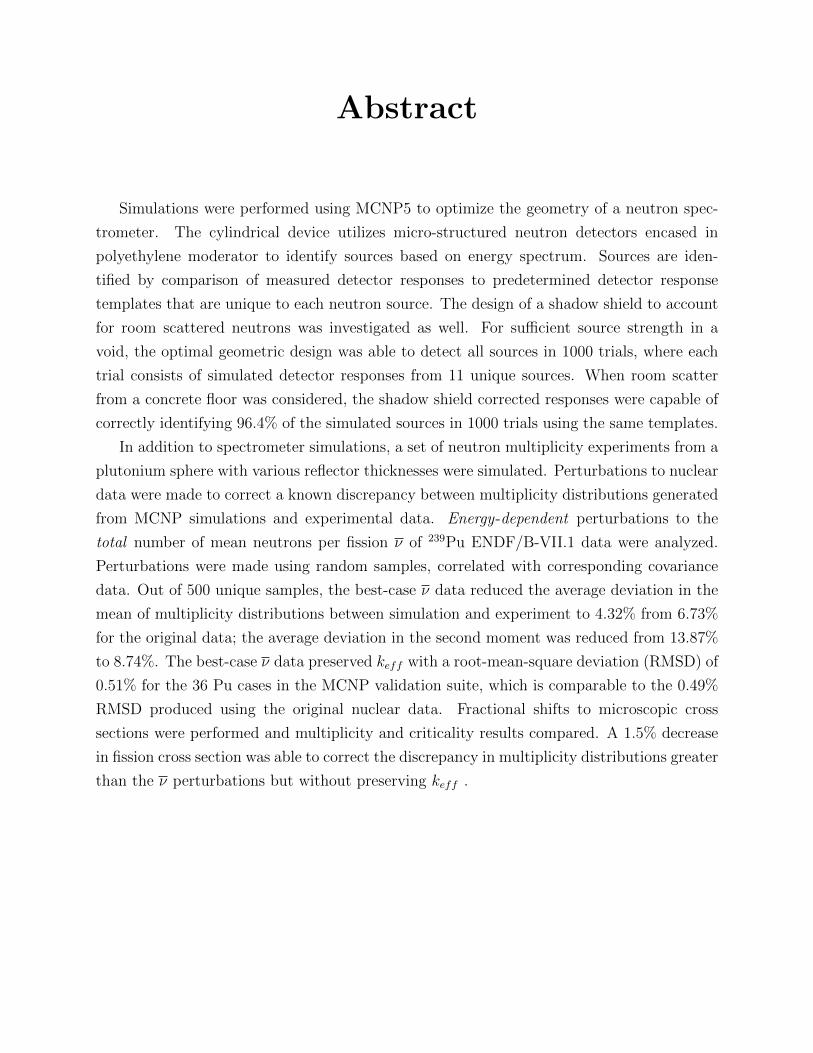
Simulations were performed using MCNP5 to optimize the geometry of a neutron spec-
trometer. The cylindrical device utilizes micro-structured neutron detectors encased in
polyethylene moderator to identify sources based on energy spectrum. Sources are iden-
tified by comparison of measured detector responses to predetermined detector response
templates that are unique to each neutron source. The design of a shadow shield to account
for room scattered neutrons was investigated as well. For sufficient source strength in a
void, the optimal geometric design was able to detect all sources in 1000 trials, where each
trial consists of simulated detector responses from 11 unique sources. When room scatter
from a concrete floor was considered, the shadow shield corrected responses were capable of
correctly identifying 96.4% of the simulated sources in 1000 trials using the same templates.
In addition to spectrometer simulations, a set of neutron multiplicity experiments from a
plutonium sphere with various reflector thicknesses were simulated. Perturbations to nuclear
data were made to correct a known discrepancy between multiplicity distributions generated
from MCNP simulations and experimental data. Energy-dependent perturbations to the
total number of mean neutrons per fission ν of 239Pu ENDF/B-VII.1 data were analyzed.
Perturbations were made using random samples, correlated with corresponding covariance
data. Out of 500 unique samples, the best-case ν data reduced the average deviation in the
mean of multiplicity distributions between simulation and experiment to 4.32% from 6.73%
for the original data; the average deviation in the second moment was reduced from 13.87%
to 8.74%. The best-case ν data preserved keff with a root-mean-square deviation (RMSD) of
0.51% for the 36 Pu cases in the MCNP validation suite, which is comparable to the 0.49%
RMSD produced using the original nuclear data. Fractional shifts to microscopic cross
sections were performed and multiplicity and criticality results compared. A 1.5% decrease
in fission cross section was able to correct the discrepancy in multiplicity distributions greater
than the ν perturbations but without preserving keff .
Table of Contents
Table of Contents iii
List of Figures vi
List of Tables ix
Acknowledgements xi
1 Introduction 11.1 A Neutron Source Identification Spectrometer . . . . . . . . . . . . . . . . . 11.2 Simulations of Multiplicity Distributions . . . . . . . . . . . . . . . . . . . . 4
2 Theory 62.1 Relevant Probability and Statistics . . . . . . . . . . . . . . . . . . . . . . . 6
2.1.1 Random Variables and Probability Distribution Functions . . . . . . 62.1.2 Expectation Values and Moments . . . . . . . . . . . . . . . . . . . . 72.1.3 Covariance and Correlation Matrices . . . . . . . . . . . . . . . . . . 82.1.4 Sample Mean and Variance . . . . . . . . . . . . . . . . . . . . . . . 82.1.5 Useful Distributions . . . . . . . . . . . . . . . . . . . . . . . . . . . 92.1.6 Generating Random Samples from a Distribution . . . . . . . . . . . 112.1.7 Generating a Set of Correlated Random Samples . . . . . . . . . . . 122.1.8 Error Propagation Formula . . . . . . . . . . . . . . . . . . . . . . . 132.1.9 χ2 Goodness-of-Fit Statistic . . . . . . . . . . . . . . . . . . . . . . . 15
2.2 Nuclear Data and Radiation Interactions . . . . . . . . . . . . . . . . . . . . 162.2.1 Attenuation of Neutral Particles . . . . . . . . . . . . . . . . . . . . . 162.2.2 Microscopic Cross Section . . . . . . . . . . . . . . . . . . . . . . . . 172.2.3 Neutron Flux Density . . . . . . . . . . . . . . . . . . . . . . . . . . 182.2.4 Effective Neutron Multiplication Factor . . . . . . . . . . . . . . . . . 192.2.5 Neutrons Released per Fission ν . . . . . . . . . . . . . . . . . . . . . 20
2.3 Monte Carlo Transport Code . . . . . . . . . . . . . . . . . . . . . . . . . . . 212.3.1 The Monte Carlo Method and MCNP . . . . . . . . . . . . . . . . . . 212.3.2 Non-Analog Variance Reduction in MCNP . . . . . . . . . . . . . . . 21
iii
3 Review of Neutron Spectrometry 243.1 The Unfolding Problem . . . . . . . . . . . . . . . . . . . . . . . . . . . . . . 24
3.1.1 The Unfolding Equation . . . . . . . . . . . . . . . . . . . . . . . . . 243.1.2 Regularizing the Set of Algebraic Equations . . . . . . . . . . . . . . 26
3.2 Solution Methods . . . . . . . . . . . . . . . . . . . . . . . . . . . . . . . . . 273.3 Neutron Spectrometer Designs . . . . . . . . . . . . . . . . . . . . . . . . . . 28
3.3.1 Single Detector Response Systems . . . . . . . . . . . . . . . . . . . . 283.3.2 Multiple Detector Response Systems . . . . . . . . . . . . . . . . . . 28
4 Simulations of a Neutron Source Identification Spectrometer 314.1 Methodology . . . . . . . . . . . . . . . . . . . . . . . . . . . . . . . . . . . 31
4.1.1 Overview . . . . . . . . . . . . . . . . . . . . . . . . . . . . . . . . . 314.1.2 Source Identification Based on a FOM . . . . . . . . . . . . . . . . . 32
4.2 MCNP5 Model . . . . . . . . . . . . . . . . . . . . . . . . . . . . . . . . . . 364.2.1 Geometry and Neutron Sources . . . . . . . . . . . . . . . . . . . . . 364.2.2 Simplified Model of Perforated Neutron Detectors . . . . . . . . . . . 374.2.3 Detector Response in MCNP5 . . . . . . . . . . . . . . . . . . . . . . 394.2.4 Boron in Circuit Boards . . . . . . . . . . . . . . . . . . . . . . . . . 404.2.5 Variance Reduction and MCNP5 Parameters . . . . . . . . . . . . . . 404.2.6 Verifying Artificial Detector Model Using MCNP6 . . . . . . . . . . . 41
4.3 Geometric Optimization . . . . . . . . . . . . . . . . . . . . . . . . . . . . . 464.3.1 Motivation . . . . . . . . . . . . . . . . . . . . . . . . . . . . . . . . . 464.3.2 Development of Objective Function . . . . . . . . . . . . . . . . . . . 504.3.3 Simulated Responses . . . . . . . . . . . . . . . . . . . . . . . . . . . 52
4.4 Automation of Simulations and Data analysis . . . . . . . . . . . . . . . . . 544.5 Corrections to the FOM for MCNP Simulations . . . . . . . . . . . . . . . . 554.6 Optimization Results . . . . . . . . . . . . . . . . . . . . . . . . . . . . . . . 56
4.6.1 Optimal Detector Spacing for a Fixed Radius . . . . . . . . . . . . . 574.6.2 Determination of Threshold Source Strength and Θ for Correct Source
Identification . . . . . . . . . . . . . . . . . . . . . . . . . . . . . . . 634.6.3 Radius of the Moderator . . . . . . . . . . . . . . . . . . . . . . . . . 694.6.4 Optimal Moderator Aspect Ratio with a Fixed Weight . . . . . . . . 70
4.7 Detecting WGPu versus 240Pu . . . . . . . . . . . . . . . . . . . . . . . . . 724.8 Shadow Shield Design and Optimization . . . . . . . . . . . . . . . . . . . . 74
4.8.1 Motivation . . . . . . . . . . . . . . . . . . . . . . . . . . . . . . . . . 744.8.2 Source Identification with Shadow Shield Measurements . . . . . . . 774.8.3 Comparison of Shield Designs . . . . . . . . . . . . . . . . . . . . . . 784.8.4 MCNP Model . . . . . . . . . . . . . . . . . . . . . . . . . . . . . . . 784.8.5 Shadow Shield Thickness . . . . . . . . . . . . . . . . . . . . . . . . . 824.8.6 Optimal Shield Location . . . . . . . . . . . . . . . . . . . . . . . . . 834.8.7 Results with Optimal Shield Design . . . . . . . . . . . . . . . . . . . 87
4.9 Conclusions, Recommendations, and Future Work . . . . . . . . . . . . . . . 91
iv

5 Simulations of Neutron Multiplicity Measurements with Perturbations toNuclear Data 935.1 Motivation . . . . . . . . . . . . . . . . . . . . . . . . . . . . . . . . . . . . . 935.2 Background . . . . . . . . . . . . . . . . . . . . . . . . . . . . . . . . . . . . 94
5.2.1 Neutron Multiplicity Distributions . . . . . . . . . . . . . . . . . . . 945.2.2 Application of Multiplicity Distributions . . . . . . . . . . . . . . . . 95
5.3 Pu Experiments and Multiplicity Measurements . . . . . . . . . . . . . . . . 975.3.1 Overview of Experimental Setup . . . . . . . . . . . . . . . . . . . . . 975.3.2 Previous Modeling Work . . . . . . . . . . . . . . . . . . . . . . . . . 98
5.4 Methodology . . . . . . . . . . . . . . . . . . . . . . . . . . . . . . . . . . . 995.4.1 Modifying Nuclear Data Files . . . . . . . . . . . . . . . . . . . . . . 995.4.2 Correlated Random Sampling of ν in ACE Files . . . . . . . . . . . . 1005.4.3 Energy-Averaged Perturbations of Capture Cross Section . . . . . . . 1025.4.4 Energy-Averaged Perturbations of Fission Cross Section . . . . . . . 1035.4.5 Quantifying Shifts in Cross Sections . . . . . . . . . . . . . . . . . . . 104
5.5 Data Generation, Simulations, and Comparison to Experimental Data . . . . 1045.6 Results for ν Perturbations . . . . . . . . . . . . . . . . . . . . . . . . . . . . 1065.7 Results of Cross Section Perturbations . . . . . . . . . . . . . . . . . . . . . 115
5.7.1 Results of Capture Cross Section Perturbations . . . . . . . . . . . . 1155.7.2 Results of Fission Cross Section Perturbations . . . . . . . . . . . . . 1205.7.3 Results of Altering both Fission and Capture . . . . . . . . . . . . . 121
5.8 Conclusions . . . . . . . . . . . . . . . . . . . . . . . . . . . . . . . . . . . . 1265.9 Summary and Suggestions for Future Work . . . . . . . . . . . . . . . . . . . 127
Bibliography 128
A Changes in Probabilities of Interaction Events 133
B Spectrometer Scripts and Codes 135
C Spectrometer MCNP Files 175
D Example Tabulated Data for Spectrometer Simulations 186
E Multiplicity Scripts and Codes 197
F Multiplicity and Criticality MCNP Input Files 247
v
List of Figures
1.1 Cylindrical neutron spectrometer with illustration of materials and possibleneutron paths . . . . . . . . . . . . . . . . . . . . . . . . . . . . . . . . . . . 3
2.1 Neutrons incident upon an infinite slab of thickness T . . . . . . . . . . . . . 17
4.1 Simulated spectrometer responses from various sources, followed by the nor-malized spectra, where the counts in each detector is divided by the counts inthe second detector. The relative standard error for all data points is < 0.5%. 33
4.2 Illustration of section of double-stacked straight-trenched detector concept,not to scale. . . . . . . . . . . . . . . . . . . . . . . . . . . . . . . . . . . . . 37
4.3 Dimensions of a unit cell of a perforated, straight-trenched detector . . . . . 424.4 Comparison of detector responses for AmBe, PuBe, and 14.1 MeV fusion
sources. All responses are normalized to second detector. All relative errorsare less that 0.7%. The dashed line indicates the artificial detectors, and thesolid line indicates an explicit MCNP6 model. . . . . . . . . . . . . . . . . . 48
4.5 Comparison of detector responses for 252Cf and 240Pu sources. All responsesare normalized to second detector. All relative errors are less that 0.7%. Thedashed line indicates the artificial detectors, and the solid line indicates anexplicit MCNP6 model. . . . . . . . . . . . . . . . . . . . . . . . . . . . . . . 49
4.6 Illustration of dimensions for axial cross section of spectrometer with Ndet = 6detectors. . . . . . . . . . . . . . . . . . . . . . . . . . . . . . . . . . . . . . 57
4.7 Comparison of various values of uniform detector spacing t for various numbersof detectors and fixed r=10cm. . . . . . . . . . . . . . . . . . . . . . . . . . 59
4.8 Comparison of Θ for different values of Ndet with optimal values of t. . . . . 604.9 Comparison of spectrometer intrinsic efficiency (εspec) and Θ for various t and
11 detectors. . . . . . . . . . . . . . . . . . . . . . . . . . . . . . . . . . . . . 614.10 Comparison of normalized spectrometer intrinsic efficiencies (εspec) and Θs for
various t and 10 and 11 detectors . . . . . . . . . . . . . . . . . . . . . . . . 624.11 Comparison of Θ and psucc, the probability of correctly identifying all sources
in a trial, for various source strengths. . . . . . . . . . . . . . . . . . . . . . 674.12 Comparison of Θ for various source strengths and Ndet. . . . . . . . . . . . . 684.13 Comparison of Θ and radius of moderator r. . . . . . . . . . . . . . . . . . . 704.14 Comparison of Θ for different geometries with a fixed value of w of 4.84 kg. . 714.15 Comparison of neutron source energy spectra for WGPu, 240Pu, and 252Cf. . 734.16 Comparison of detector spectra from different fission neutron sources. . . . . 74
vi

4.17 Illustration of the two shadow shield measurements. Several possible neu-tron paths are illustrated: (A) neutrons deflected or absorbed in the shield,(B) neutrons scattered off of the environment entering the front of the spec-trometer without interacting in the shield, (C line-of-site neutrons, and (D)neutrons scattered off of the environment entering the front of the device. . 76
4.18 Geometry for room shine scenario. . . . . . . . . . . . . . . . . . . . . . . . . 794.19 Dimensions for room shine scenario. . . . . . . . . . . . . . . . . . . . . . . . 804.20 Comparison of room-scatter spectra with no correction and void spectra. . . 844.21 Axial slice of shadow shield with dimension labels. . . . . . . . . . . . . . . . 844.22 Comparison of net detector spectra for various shadow shield thicknesses. . . 854.23 Comparison of net detector spectra at last few detector positions. . . . . . . 864.24 Comparison of net detector spectra with void spectra for a 20-cm thick shadow
shield at a location of z = 0.5. . . . . . . . . . . . . . . . . . . . . . . . . . . 884.25 Comparison of net spectra with room scatter included and void for various z,
using a 20-cm thick shadow shield. . . . . . . . . . . . . . . . . . . . . . . . 894.26 Comparison of the effect of room type on detector spectra. . . . . . . . . . . 91
5.1 Illustration of construction of a multiplicity distribution from a neutron pulsetrain. Multiplicity is the number of neutrons detected in one gate width;frequency is the number of gates with a certain multiplicity in counting timeT . . . . . . . . . . . . . . . . . . . . . . . . . . . . . . . . . . . . . . . . . . 95
5.2 Illustration of multiplicity experiments (not to scale). . . . . . . . . . . . . . 975.3 Semi-log plot of ν versus energy for trial 303 and ENDF/B-VII.1. . . . . . . 1105.4 Plot of ν versus energy for trial 303 and ENDF/B-VII.1 for energies 85 to 150
eV. . . . . . . . . . . . . . . . . . . . . . . . . . . . . . . . . . . . . . . . . . 1115.5 Plot of number of standard deviations that trial 303 shifted ν from original
ENDF/B-VII.1 data by energy bin. . . . . . . . . . . . . . . . . . . . . . . . 1125.6 Plot of percent deviation of ν for trial 303 from the original ENDF/B-VII.1
data at each evaluated energy. . . . . . . . . . . . . . . . . . . . . . . . . . . 1125.7 Comparison of multiplicity distributions using original ENDF/B-VII.1 data
and experimental multiplicity distributions. Distributions are for (A) bare Pusphere, (B) 0.5-cm reflector, (C) 1.0-cm reflector, (D) 1.5-cm reflector, and(E) 3.0-cm reflector. . . . . . . . . . . . . . . . . . . . . . . . . . . . . . . . 113
5.8 Comparison of multiplicity distributions using trial 303 (modified ENDF/B-VII.1 ν data) and experimental multiplicity distributions. Distributions arefor (A) bare Pu sphere, (B) 0.5-cm reflector, (C) 1.0-cm reflector, (D) 1.5-cmreflector, and (E) 3.0-cm reflector. . . . . . . . . . . . . . . . . . . . . . . . . 114
5.9 Comparison of multiplicity distributions for the 3.0-cm polyethylene reflectedsphere of Pu. . . . . . . . . . . . . . . . . . . . . . . . . . . . . . . . . . . . 117
5.10 Comparison of multiplicity distributions for -1.14% reduced energy averagedν and experimental multiplicity distributions. Distributions are for (A) barePu sphere, (B) 0.5-cm reflector, (C) 1.0-cm reflector, (D) 1.5-cm reflector,and (E) 3.0-cm reflector. . . . . . . . . . . . . . . . . . . . . . . . . . . . . . 123
vii

5.11 Comparison of multiplicity distributions for 16% increased σc from case 1 andexperimental multiplicity distributions. Distributions are for (A) bare Pusphere, (B) 0.5-cm reflector, (C) 1.0-cm reflector, (D) 1.5-cm reflector, and(E) 3.0-cm reflector. . . . . . . . . . . . . . . . . . . . . . . . . . . . . . . . 124
5.12 A comparison of multiplicity distributions for σf reduced 1.5% and experi-mental multiplicity distributions; σs was increased to compensate for changesin σf , as described in case 4 of Section 5.4.3. Distributions are for (A) barePu sphere, (B) 0.5-cm reflector, (C) 1.0-cm reflector, (D) 1.5-cm reflector,and (E) 3.0-cm reflector. . . . . . . . . . . . . . . . . . . . . . . . . . . . . . 125
viii
List of Tables
4.1 Neutron sources used for spectrometer simulations. . . . . . . . . . . . . . . 364.2 Geometric specifications for unit cell of a perforated, straight-trenched device. 434.3 Crystalline LiF (ρ = 2.635g cm−3) material composition for MCNP6 model. . 444.4 Natural Si (ρ = 2.3290g cm−3) material composition for MCNP6 model. . . . 444.5 FR4 printed circuit board (ρ = 2.635g cm−3) material composition for MCNP6
model. . . . . . . . . . . . . . . . . . . . . . . . . . . . . . . . . . . . . . . . 444.6 Comparison of detector responses generated using artificial MCNP5 and ex-
plicit MCNP6 detector models. The detector indexing is i = Position /( 3.0 cm).Errors are reported as absolute. . . . . . . . . . . . . . . . . . . . . . . . . . 47
4.7 Comparison of optimal value of Θ with respect to t for the values of Ndet fromFig. 4.7. . . . . . . . . . . . . . . . . . . . . . . . . . . . . . . . . . . . . . . 58
4.8 Comparison of Θ and psucc, the probability of correctly identifying all sourcesin a trial, for various source values of total incident neutrons S0. . . . . . . . 65
4.9 Comparison of σ(∆(n)min), Θ, and S0 for a spectrometer with 11 detectors, r = 10
cm, and t = 3.5 cm. Note, σ(∆(n)min) here is the sample standard deviation for
∆(n)min, not the standard error in the mean of the ∆(n)
min σ(Θ). The relation is
σ(∆(n)min) =
√Ncorrσ(Θ). . . . . . . . . . . . . . . . . . . . . . . . . . . . . . . 66
4.10 Comparison of aspect ratios and Θ for a variety of Ndet and a fixed weight ofw at 4.84 kg. . . . . . . . . . . . . . . . . . . . . . . . . . . . . . . . . . . . 72
4.11 Concrete (ρ = 2.70 g cm−3) material composition for room scatter simulations. 804.12 Comparison of χ2
red values for different shadow shield thicknesses. . . . . . . 854.13 Comparison of χ2
red for different locations of a 20-cm thick shadow shield. . . 874.14 Source identification data with room scatter from an enclosed room. . . . . . 904.15 Source identification data with room scatter from a concrete floor. . . . . . . 91
5.1 FOM and χ2 values for ten trials with lowest FOM values, and original andshifted ENDF/B-VII.1 data. . . . . . . . . . . . . . . . . . . . . . . . . . . 107
5.2 Comparison of keff for different data with the MCNP criticality validationbenchmark suite. . . . . . . . . . . . . . . . . . . . . . . . . . . . . . . . . . 108
5.3 Comparison of first and second multiplicity moments for different thicknessesof polyethylene reflector. . . . . . . . . . . . . . . . . . . . . . . . . . . . . 109
5.4 A comparison of results for case 1 where σc was increased and σt was increasedto compensate for the change, at each energy. . . . . . . . . . . . . . . . . . 117
ix
5.5 A comparison of results for case 2 in which σc was increased and σs wasincreased to keep the ratio of scattering to σt the same as in the original data;σt was increased to compensate for the changes in σc and σs. . . . . . . . . . 118
5.6 A comparison of results for case 3 in which σc was increased and σs wasincreased to keep the ratio of σc to σs the same as in the original data; σt wasincreased to compensate for the change in σc and σs. . . . . . . . . . . . . . 118
5.7 A comparison of results for case 4 in which σc was increased and σs wasdecreased to keep σt the same as in the original data, for neutron energiesgreater than 1 keV. . . . . . . . . . . . . . . . . . . . . . . . . . . . . . . . . 119
5.8 A comparison of results for case 1 in which σc was increased and σs wasdecreased to keep σt the same. Changes were made to cross sections forneutron energies above Ecut. . . . . . . . . . . . . . . . . . . . . . . . . . . 119
5.9 A comparison of results for reduced σf with σt reduced to compensate for thechanges, as described in case 1. . . . . . . . . . . . . . . . . . . . . . . . . . 120
5.10 A comparison of results for σf alterations of case 4. Cross sections were alteredfor neutron energies greater than 1 keV. . . . . . . . . . . . . . . . . . . . . 121
5.11 A comparison of the results for case 5 in which σc was increased and σf wasdecreased to keep σt the same as in the original data, for energies above Ecut. 121
D.1 Simulation data for spectrometer with geometry parameters Ndet = 11, r =10.00 cm, and t = 2.00 cm. . . . . . . . . . . . . . . . . . . . . . . . . . . . . 187
D.2 Simulation data for spectrometer with geometry parameters Ndet = 11, r =10.00 cm, and t = 3.00 cm. . . . . . . . . . . . . . . . . . . . . . . . . . . . . 188
D.3 Simulation data for spectrometer with geometry parameters Ndet = 11, r =10.00 cm, and t = 3.50 cm. . . . . . . . . . . . . . . . . . . . . . . . . . . . . 189
D.4 Simulation data for spectrometer with geometry parameters Ndet = 11, r =10.00 cm, and t = 4.00 cm. . . . . . . . . . . . . . . . . . . . . . . . . . . . . 190
D.5 Simulation data for spectrometer with geometry parameters Ndet = 11, r =10.00 cm, and t = 4.50 cm. . . . . . . . . . . . . . . . . . . . . . . . . . . . . 191
D.6 Simulation data for spectrometer with geometry parameters Ndet = 11, r =10.00 cm, and t = 5.00 cm. . . . . . . . . . . . . . . . . . . . . . . . . . . . . 192
D.7 Simulated counting data from point sources of strength s0 = 109 n cm−2 abovea concrete floor; FOMmin and FOMmin + represent the lowest and secondlowest FOM values, respectively, and Cnet
i is the room shine net spectra, i.e.,Cneti = C ns
i − Csi . Values in the table of “Correct” and “Inorrect” indicate
whether the source was correctly identified. . . . . . . . . . . . . . . . . . . . 193
x
Acknowledgments
First and foremost, I would like to thank Dr. Shultis for taking me back as a graduatestudent. His constant wisdom, patience, and easy-going personality made this a relativelypainless process. I would like to acknowledge Dr. C.J. Solomon at LANL for his mentorshipand assistance while producing this work. In addition, I would like to thank my parents for20 some odd years of guidance and support, as well as for embracing my choice to departthe farmstead to pursue academic ventures. Finally, I would like to thank Madeline Millerfor accepting two years of long distance, albeit they were great years, without professing asingle complaint on the matter.
This research was performed using funding received from the DOE Office of Nuclear En-ergy’s Nuclear Energy University Programs. The spectrometer design work was supported inpart by the Defense Threat Reduction Agency (DTRA) contracts DTRA-12-C-0004, DTRA-01-03-C-0051, and DTRA-01-02-0-0067-003.
xi
Chapter 1
Introduction
This thesis discusses results of simulations related to two unique applications of neutron
measurements: neutron spectrometry and multiplicity counting. Chapter 2 provides the
necessary statistics and theory of radiation to understand the computations and modeling
for the spectrometer and nuclear data studies. A summary of previous methods and designs
in neutron spectrometry are given in Chapter 3. Chapter 4 focuses on the spectrometer design
methodology for this work, as well as presenting optimization results. Finally, nuclear data
perturbations and simulated multiplicity distribution results are discussed in Chapter 5.
1.1 A Neutron Source Identification Spectrometer
As nuclear safeguards become increasingly important, a method for quickly discriminating
among different types of neutron sources is vital. The measurement and rapid identification
of the distribution of the kinetic energy of neutrons has seen broad study and application
since the 1960s with the invention of portable neutron spectrometers. The primary utility
of neutron spectrometry has been the ability to estimate the dose experienced by radiation
workers. Neutron spectrometry has seen resent resurgence in the field of nuclear safeguards.
The control and identification of special nuclear material is important for global security,
and the ability to quantify fissionable materials is crucial for fuel reprocessing and modern
reactor designs to be viable. Research in design of spectrometers for dosimetry has provided
a framework of methods for determining neutron energy spectra based on the theory of
unfolding the original spectra from a set of energy-dependant measurements. However,
unfolding is a complex, subjective, and generally unstable numerical process. A spectrometer
that does not depend on unfolding neutron spectra has been developed at Kansas State
University. The device and methodology has been demonstrated to be effective at identifying
neutron sources based on direct analysis of energy-dependent measurements [Cooper et al.,
1

2011]. This neutron source identification spectrometer is optimized and evaluated via Monte
Carlo simulations in this work.
The neutron source identification spectrometer design in this thesis uses micro-structured
semiconductor neutron detectors (MSNDs) described by Shultis and McGregor [2009]. These
MSNDs are efficient at detecting thermal-energy neutrons (with kinetic energy near 0.025
eV) and are capable of 43% efficiency through summation of the output from two stacked, off-
set detection volumes [Bellinger et al., 2010]. The thickness of the detection volume (parallel
to the direction of irradiation) for a double-stacked device is around 0.1 cm deep, a desir-
able feature for creating a compact spectrometer. The cross sectional area of the devices
can be increased to the necessary areas by placing multiple MSNDs together and summing
their outputs. In addition to the small thickness and high efficiency, the semiconductor de-
tectors are made primarily of silicon, which has a relatively low neutron interaction cross
section. This results in detectors that cause minimal perturbance of the neutron field at
non-thermal energies. The low perturbance allows multiple detectors to be placed within
the same moderator and provide multiple energy-dependent data points from a single geo-
metric configuration and measurement. Not needing multiple time-consuming measurements
significantly improves the overall speed of source identification.
The geometry of the spectrometer consists of an array of MSNDs placed along the axis of a
cylinder of high density polyethylene (HDPE) moderator. A sheet of Cd is placed behind each
detector to prevent backscattered thermal neutrons from being detected. Figure 1.1 depicts
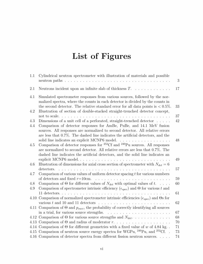
the basic geometric features of a spectrometer consisting of 11 thermal neutron detectors;
Detail View A provides an illustration of materials and possible neutron trajectories through
the spectrometer. As neutrons travel through the moderator, they lose kinetic energy through
scattering collisions. If a neutron slows to thermal energies within a detection volume, the
probability of absorption and identification at position is extremely high. For neutrons with
higher initial energies, more scattering collisions are required to reach thermal energy, on
average. This leads to higher energy neutrons having a higher probability of being absorbed
at deeper positions in the spectrometer. Thus, each detector position has a particular energy
of incident neutrons on the spectrometer that it is most likely to detect. It is noted that
because of the stochastic behavior of neutron scattering, each detector is sensitive to a range
of energies, i.e., a fast, mono-energetic source would produce counts in multiple detectors.
The sheets of Cd help to limit the range of energies each detector is sensitive to by preventing
backscattered thermal neutrons from entering detector volumes from the back.
Because each detector position is sensitive to a particular energy, with some distribution
about that energy, the set of detector responses are unique for a particular energy distribution
of incident neutrons. Because all bare neutron sources have a particular energy distribution,
2
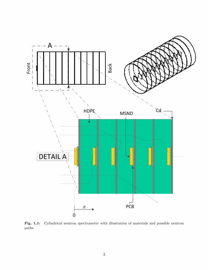
HDPE MSND
x
0
Cd
PCB
A
DETAIL A
Fro
nt
Bac
k
Fig. 1.1: Cylindrical neutron spectrometer with illustration of materials and possible neutronpaths
3
the expected response in each detector per incident neutron is unique to a source. By
normalizing the responses in all of the responses to one detector position, the dependence
on source strength can be removed. Thus, if room scatter can be accounted for, a library
of normalized responses for different sources can be created. An experimental measured
response is then compared to the different responses in the library to identify the most likely
source. The source library can be created from either experimental measurements or accurate
simulations. Comparison of a measured response to the library templates is computationally
very efficient and simple, which leads to rapid source identification by a low-power on-board
microprocessor; post-processing of measured data and user input required for unfolding is
not needed with this template matching method.
First, this work develops a method to quantify the quality of a neutron spectrometer via
an objective function based on the statistical confidence of neutron source identifications.
This objective function is then applied to the spectrometer through many Monte Carlo
simulations to optimize the geometry of the device. The Monte Carlo N-Particle (MCNP5)
code was used for these simulations. Simulation studies are also performed to determine
the design and effect of location of a shadow shield to account for roomshine. The shadow
shield is a known method for calibrating neutron spectrometry experiments that attempts to
remove the effect of room-scattered neutrons. Remarks and considerations for future work
for the source identification spectrometer are then discussed.
1.2 Simulations of Multiplicity Distributions
The second main focus of this work applies MCNP simulations to a different field of neutron
measurements. In particular, use of time dependent data from neutron measurements to
construct multiplicity distributions is investigated. A neutron multiplicity distribution de-
picts the probability of a particular number of neutrons created within a multiplying system
being measured over some fixed short amount of time, and is discussed more thoroughly in
Chapter 5. Multiplicity distributions are based on coincident events, and they are used to
quantify neutron multiplication parameters in a system. Multiplicity distributions have seen
their main application in the passive assay of subcritical multiplying systems, specifically
quantifying the fissionable material in a device. The validation of simulation tools for mod-
eling such measurements is of great importance to nuclear safeguards and control of special
nuclear materials. Monte Carlo modeling is known to inaccurately recreate a particular set of
relatively simple multiplicity experiments of reflected plutonium spheres, consisting mostly
of the isotope 239Pu [Mattingly, 2009]. The cause of this discrepancy has been narrowed
down to the nuclear data [Miller et al., 2010].
4
Investigation of these experiments has an arguably more important auxiliary benefit.
When nuclear data are tabulated for use in simulation codes, there are adjustments performed
to the original experimental data with the interest of matching the results of benchmark
criticality experiments. The data are not well validated against subcritical experiments.
The results in this work demonstrate that subcritical results need to be considered when
nuclear data evaluations are performed to create simulation tools that can correctly model
such systems. The framework for the work herein can be applied to develop a set of data for
a specific task, in this case highly multiplying, fast, subcritical systems.
For this work, perturbations are made to nuclear data to correct the discrepancy between
experimental and simulated multiplicity experiments. The focus of perturbations is correctly
preserving statistical correlations and uncertainties from experimental measurements of the
nuclear data. The primary nuclear data type of interest is the average number of neutrons
produced per fission ν. Energy-dependent perturbations are made to help conserve the
overall balance of neutrons in the system, as increases at one energy may be compensated
by decreases at another energy. Additionally, energy-averaged shifts to cross sections are
analyzed to determine the sensitivity of the system to ν , relative to cross section alterations.
In Chapter 5, a brief overview of neutron multiplicity distributions is given. Then,
the experiments to be analyzed and previous simulation work are described. The methods
for generating correlated, perturbed nuclear data and comparing the results of multiplicity
simulations for the perturbed data sets are discussed. Perturbations were made to nuclear
data for 239Pu and simulations of multiplicity distributions performed to determine the effect
and correction caused by the individual perturbations. Simulations were performed using
the sets of perturbed data as the input for the MCNP5 code with special subroutines for
studying subcritical systems. The reflected plutonium spheres are modeled explicitly and
neutron multiplicity distributions are generated using a post-processing script. Results are
discussed and compared.
5
Chapter 2
Theory
2.1 Relevant Probability and Statistics
2.1.1 Random Variables and Probability Distribution Functions
A continuous random variable is a variable that maps the occurrence of a particular event
onto a set of real numbers, in a one-to-one manner [Hogg et al., 2013]. The value of the
random variable is in general unknown until a realization (i.e., an observation or sampling) of
the variable occurs. Typically upper-case characters are used to indicate a random variable,
whereas lower-case is used to indicate the value of a sample on the variable. It is noted that
samples are a random variable themselves until realization occurs [Hogg et al., 2013], but in
this work samples refer to the value of realizations on a random variable. The probability
of the random variable taking on a particular value can be known in advance and is defined
using probability distribution functions. The cumulative distribution function (CDF) is a
non-decreasing, positive function F (x) whose values lie between 0 and 1. For a random
variable X with CDF F (x), the value of F (x) represents the probability that X will have a
value less than or equal to x (in standard notation F (x) = P (X ≤ x)). Related to the CDF,
is the probability density function (PDF). The PDF f(x) is defined as
f(x) =dF (X)
dx. (2.1)
Explicitly, the value f(x) dx represents the probability of finding X in dx about x. Therefore,
normalization requires ∫ ∞−∞
f(x) dx = 1. (2.2)
6
From the above definitions, it is straightforward that the PDF can be used to compute the
probability of finding X between a and b, where a < b and a, b ∈ SX , as
P (a < x < b) =
∫ b
a
f(x) dx. (2.3)
It is noted that the PDF and CDF are defined for all real numbers by definition, even though
the random variable may be defined for some subset of all real numbers. The support (SX
above) of a random variable is defined as the points in the domain of a random variable for
which the probability is positive; in this work the supports of random variables are given to
identify their domain; it is assumed the PDF is zero elsewhere. The discussion in this section
is for continuous random variables but can be easily extended to discrete random variables,
as discussed in literature [Hogg et al., 2013; Shultis and Dunn, 2011].
2.1.2 Expectation Values and Moments
An expectation value for a function g(x) is defined as
E[g(x)] =
∫ ∞−∞
g(x)f(x) dx, (2.4)
where f(x) is the PDF for the random variable X. The expected value of a function rep-
resents the mean, or average, value of the function that would be calculated using repeated
observed values of x. Some special expectations are useful to define the shape and behavior
of a distributions, in particular the moments and their combinations. The n-th moment of
a PDF is defined as
Mn = E(xn) =
∫ ∞−∞
xn, f(x) dx. (2.5)
The first moment is the mean value of the random variable X, notated as µ. A particularly
useful combination of moments is defined as the variance, σ2, which can be shown to be [Hogg
et al., 2013]
σ2 =
∫ ∞−∞
(x− µ)2 f(x) dx = M2 − (M1)2. (2.6)
The square root of the variance is defined as the standard deviation. The standard deviation
is useful in defining statistical confidence intervals about the mean.
7
2.1.3 Covariance and Correlation Matrices
Consider a set of N dependent random variables Xi : i = 1, 2, . . . , N . The covariance
between two of any variables in this set, Xi and Xj, is
Cov(Xi, Xj) = E(XiXj)− E(Xi)E(Xj). (2.7)
From the above definition of variance, Cov(Xi, Xi) = σ2(i). From the covariance between
each all pairs of terms, a covariance matrix Σ is formed as
Σij = Cov(Xi, Xj) : i = 1, 2, . . . , N ; j = 1, 2, . . . , N. (2.8)
The syntax here is Σij is the matrix element of the i-th row and j-th column of a matrix Σ.
Directly related to a covariance matrix Σ is its correlation matrix, C, with elements, known
as correlation coefficients,
Cij =Σij√ΣiiΣjj
: i = 1, 2, . . . , N ; j = 1, 2, . . . , N. (2.9)
The correlation matrix provides a measure of the interdependence between the i-th and j-th
variable, i.e., on average if the value of one variable is observed, the correlation coefficient
provides the expected behavior of the second. All values of the correlation matrix are between
-1 and 1. A negative value indicates that if the probability of observing large values of the i-
th variable is high, then the second variable is expected to be small, on average; the converse
is also true. Positive correlation coefficients indicate that if the probability of observing
a large value of a variable is high, then the probability of observing large values of the
second variable is also high; again, the converse is also true. The magnitudes of the values
indicate the strength of the correlation, with the diagonal terms being the strongest at 1
(the correlation of a variable with itself is perfect). A set of independent variables would
have zero for all off-diagonal terms of C.
2.1.4 Sample Mean and Variance
Often, the exact moments of a distribution (population moments) are unknown because the
CDF and PDF can be complicated or unknown; population moments can also be undefined
if the integrals in the previous section diverge. However, samples from a distribution can
be used to estimate the population moments. Here, a set of samples is formally a set of
independent, random observations of a random variable with some distribution. The sample
mean X is simply the average of a set of N discrete samples xi : i = 1, 2, . . . , N on the
8
random variable X with PDF f(x), i.e.,
x =1
N
N∑i=1
xi. (2.10)
Similarly, the sample variance s2 is given by
s2 =1
N − 1
N∑i=1
(xi − x)2. (2.11)
The subtraction of one from N in the above equation comes as a result of a loss of a
degree of freedom by approximating the population mean with the sample mean [Shultis
and Dunn, 2011]. The sample mean and variance can be shown to be unbiased estimates of
the population mean and variance, respectively [Hogg et al., 2013]. An estimator T is an
unbiased estimator of Y if E(T ) = Y ; an estimate is just the realization of an estimator T .
It can also be shown that as N →∞, the sample mean and variance converge in probability
to the population mean and variance [Hogg et al., 2013]. It is noted that the notation for
sample and population statistics is poor (particularly for the variance), where population
statistics are discussed and notated, where sample statistics are actually applied.
2.1.5 Useful Distributions
Several distributions are used throughout this work. The PDFs for these distributions are
stated here with justification for application. In all cases, the random variable of interest is
X with PDF f(x; θ), where θ is one or more distribution parameters required to fully define
the distribution. Derivations, sampling methods, and other relations for these distributions
can be found in literature [Shultis and Dunn, 2011; Press et al., 1992].
Binomial Distribution
The binomial distribution has application for a sequence of discreet, independent random
trials which have a binomial outcome, i.e., either the outcome occurs or does not occur, with
the same probability of success p for each trial. Radiation counting measurements have a
binary outcome, i.e., either a count was made or not, so the number of counts observed in a
detector can be modeled as a binomial distributed variable. The number of successes X in
N independent trials, with probability of success in each trial p, is described as
f(x; p,N) =N !
(N − x)!x!px(1− p)N−x x = 0, 1, . . . , N. (2.12)
9
Poisson Distribution
The Poisson distribution is a discreet distribution that is useful for describing independent,
identical trials that have a low probability of success in each trial, where the number of trials is
large (usually the number of trials occurs over some relatively large, fixed time interval). For
a binomial distributed variable, if the value of N is very large with a small value of p, then the
Poisson distribution is a good approximation for the binomial distribution; the approximation
is applicable for N & 20, provided that Np < 5 [Shultis and Dunn, 2011]. Radiation counting
measurements can be appropriately modeled as a Poisson process [Tsoulfanidis, 1995]. The
distribution is fully-defined by the mean, µ, of the distribution, which is also the rate of
successful trials occurring. The number of successful trials X has the distribution:
f(x;µ) =µxe−µ
x!x = 0, 1, . . . . (2.13)
Unit Uniform Distribution
The unit uniform distribution is for a continuous random variable X between 0 and 1 ex-
clusive, with equal probability of occurrence at each X. The unit uniform distribution has
utility in sampling pseudo-random numbers from other distributions. The unit uniform
distribution has no distribution parameters and PDF
f(x) = 1 x ∈ (0, 1). (2.14)
Chi-squared Distribution
The χ2 distribution is for continuous random variables X defined over (0,∞). The distribu-
tion has application in optimization schemes and hypothesis testing. The degrees of freedom,
r, is the mean of X and used to fully define the distribution as
f(x; r) =1
Γ(r/2)2r/2x
r/2−1 e−x/2 x ∈ (0,∞), (2.15)
where Γ is the standard gamma function [Hogg et al., 2013]; for integers α, Γ(α) = (α− 1)!.
Gaussian (Normal) Distribution
The Gaussian (normal) distribution is for continuous random variables X ∈ (∞,∞). Al-
though it has many applications, its primary use in this work is for confidence intervals
based on the central limit theorem, as discussed in Hogg et al. [2013]. It can also used to
approximate binomial and Poisson distributions accurately in some cases. The distribution
10
is fully-defined by its mean µ and variance σ2, notated as N(µ, σ2), with PDF
f(x;µ, σ2) =1√2πσ
e−(µ−N)2/(2σ2) x ∈ (−∞,∞). (2.16)
The multivariate normal distribution is more complicated, but can be used to fully described
the distribution of multiple variables which have normal distributions with different means,
variances, and correlation between variables; the mean of each variable and the correlation
matrix fully defines the multivariate normal distribution.
2.1.6 Generating Random Samples from a Distribution
In any Monte Carlo simulation, it is necessary to sample random numbers from various
distributions. There have been many algorithms developed for efficiently sampling pseudo-
random numbers from a unit uniform distribution [Shultis and Dunn, 2011; Press et al.,
1992]. The unit uniform distribution for a random variable U has a PDF defined as fU(u) =
1, u ∈ [0, 1]. The CDF of this distribution is given by FU(u) = u, u ∈ [0, 1]. Since numbers
can efficiently be sampled from this distribution, it is useful to know the transformation
between random variables that allows for a variable with a uniform distribution to take on
any other distribution.
To determine the transformation, consider a continuous random variable X defined to be
the transformation X = F−1(U), where F−1(y) is the solution to the equation F (x) = y, for
any continuous CDF F (x). The goal is to determine the distribution of X, i.e. FX(x), and
if it is F (X), then the transformation performs the desired goal. Because F is a CDF, it
is a monotonically non-decreasing function between 0 and 1, therefore the relation between
X and U is one-to-one. Transformations between variables without a one-to-one relation
require regions of the support to be analyzed individually, as demonstrated in [Hogg et al.,
2013]. Since the transformation is one-to-one, the distribution of X is given by
FX(x) = P (X ≤ x) = P (F−1(U) ≤ x). (2.17)
Applying F to both sides of the inequality in the right most term yields
FX(x) = P (F [F−1(U)] ≤ F (x)) = P (U ≤ F (x)). (2.18)
But the probability of U being less than some value is simply the CDF of U . The CDF of
U is FU(u) = u, therefore:
FX(x) = P (U ≤ F (x)) = FU [F (X)] = F (X). (2.19)
11
Hence, the distribution of X is the CDF of interest F , which had no constraints other
than continuity. Since samples from a distribution are distributed with that distribution,
samples from the unit uniform distribution can be transformed to create samples from an-
other distribution by simply applying the inverse CDF. There are many efficient sampling
techniques developed for when the inverse does not exist [Hogg et al., 2013; Shultis and
Dunn, 2011].
2.1.7 Generating a Set of Correlated Random Samples
Normally-distributed, independent random variables, and samples of them, can be correlated
using data from a corresponding covariance matrix (with corresponding correlation matrix).
In general, to correlate a vector of normally distributed random variables using a N × N
correlation matrix C, a decomposition of the form [Rousseuw and Molenberghs, 1993]
VVT = C. (2.20)
is needed. Here V, with transpose VT , is any matrix that obeys the above equation, and C
is the correlation matrix associated with the set of data that is being sampled.
Once a matrix V is found, a vector R of n independent, normally-distributed random
numbers is correlated via [Rousseuw and Molenberghs, 1993]
R = VR. (2.21)
where R is the vector of correlated random numbers. The vector R is sampled from the
standard normal distribution, i.e., N(0, 1), and then modified to match the desired mean
and variance after correlation [Rousseuw and Molenberghs, 1993].
There are multiple types of decomposition that produce a V that is valid for Eq. (2.20).
Two common decompositions for correlated sampling are Cholesky and eigenvalue decom-
positions; the latter is more robust. For the Cholesky decomposition of a matrix C, V in
Eq. (2.21) is a lower-triangular (or symmetric upper-triangular) matrix. In an eigenvalue
decomposition of a matrix C, V of Eq. (2.21) takes the form
V = QD. (2.22)
Here, Q is a matrix where the j-th column vector represents the orthonormal eigenvector
corresponding to the j-th eigenvalue, λj, of the matrix C. The matrix D is a diagonal
matrix with the j-th diagonal element Djj =√λj. The eigenvalue decomposition may
require orthogonalization after decomposition if C contains degenerate (repeated) eigenval-
12
ues [Rousseuw and Molenberghs, 1993]. For an intuitive understanding of how these methods
sample from the correlation matrix, consider that the matrix Q is an orthonormal basis for
C. Thus, the multiplication VR is transforming the vector R into the basis of Q, such that
the distribution of variables in R is now the multivariate normal distribution with correlation
matrix C.
Cholesky decomposition is only valid for symmetric, positive-definite (PD) matrices, but
the eigenvalue decomposition described above is valid for (at least) positive-semidefinite
(PSD) matrices [Rousseuw and Molenberghs, 1993]. A matrix A is PD if XTAX > 0, for
all real vectors X; the matrix A is PSD if XTAX ≥ 0. For the eigenvalue decomposition, if
C is non-PSD the eigenvalues will be negative, resulting in non-real elements of D. A true
covariance matrix is PD, but the statistical techniques used to estimate covariance matrices
from observed data can lead to PSD and non-PSD matrices [Rousseuw and Molenberghs,
1993]. A fix-up method can be applied to correct non-PSD matrices using the eigenvalue
decomposition method. The fix-up method generates a modified C that is PSD given by
C ′ = (QD ′)(QD ′)T. (2.23)
In the above equation, D′ is a diagonal matrix with matrix elements: D′jj =√|λj|. Q is the
same orthonormal eigenvector matrix from the initial decomposition in Eq. (2.22).1
The now PSD matrix C ′ is then transformed into a correlation matrix such that the
diagonal elements are all unity, i.e.,
Cij =C ′ij√C ′ii C
′jj
(2.24)
The new correlation matrix, C, has different off-diagonal (co-relation) values than the original
correlation matrix. However, for a C with negative eigenvalues relatively small in magnitude,
the new off-diagonal elements change minimally from the original values. The new matrix
C can then be decomposed to find a V for sampling.
2.1.8 Error Propagation Formula
It is often of interest to determine the uncertainty, stochastic or systematic, in a computed
result. The uncertainty in a computed result comes directly from the uncertainty in the
1Although the elements of D in the original decomposition are complex, numerical eigenvalue decom-position methods (e.g. those in Press et al. [1992]) determine the eigenvalues (i.e., λi = (DTD)ii) andeigenvectors of a matrix, rather than the decomposition given in Eq. (2.22). Thus, the matrix of eigenvectorsQ and eigenvalues can be obtained from a non-PSD matrix.
13
observed values of the variables used to calculate it. If a functional relation between the
observed variables and the final result is known, then the error propagation equation provides
a method of approximating the uncertainties in the result, based on the independent variables
the result depends on [Dunn, 2005].
The following derivation of the general error propagation equation is for independent
distributed statistical errors, but the result can be directly applied to independent systematic
errors; the requirement in both cases is that the observed variables are generally distributed
near the observed values (e.g., normally distributed) [Dunn, 2005].
Consider a result f that is a function of a vector of n independent random variables
X = Xi : i = 1, 2, . . . , n, i.e., f = f(X). A random variable is simply a variable whose
value is unknown before observation and follows some distribution. Although there are some
special cases [Dunn, 2005], in general the exact relation between uncertainties of independent
observed variables and a functional result is unknown. An approximation is introduced by
expanding f as a first order Taylor polynomial [Dunn, 2005], i.e.,
f(X) ≈ f(Xobs) +n∑i=1
∂f
∂Xi
(Xi −Xi,obs). (2.25)
In the above equation, the vector Xobs represents the observed values of each variable Xi
used to compute the result f . For a linear combination of independent random variables,
T =∑n
i=1 aiYi, with combination coefficients ai, the variance can be shown to be [Hogg
et al., 2013]
σ2(T ) =n∑i=1
a2iσ
2(Yi) (2.26)
With the assumption all variances are defined.
In Eq. (2.25), f(X) is written as a linear combination with ai = ∂f/∂Xi and a constant
term f(Xobs). The constant term does not contribute to the variance σ2[f(X)]. Combining
these results with Eq. (2.26) yields the result for any X near Xobs (to first order):
σ(f) =
√(∂f
∂X1
σ(X1)
)2
+
(∂f
∂X2
σ(X2)
)2
+ · · ·+(∂f
∂Xn
σ(Xn)
)2
, (2.27)
where the square root has been taken to yield the standard deviation of f , σ(f), about
the observed value Xobs. The above equation is referred to as the general formula for error
propagation and can be applied to determine the uncertainty about any observed value; lower
case variables have been used to indicate that this result applies to any observed variables,
not exclusively to stochastic errors. The truncation error introduced by the first order Taylor
14
approximation is relatively small because the uncertainties are generally assumed to be small.
This approximation may be very poor, depending on the functional form of f [Taylor, 1997].
2.1.9 χ2 Goodness-of-Fit Statistic
A chi-squared goodness-of-fit statistic can be used to compare the accuracy of a set of
statistical observed data to some reference set of data (e.g. an exact solution or experimental
data). A statistic is simply a function of a set of random samples on random variables that
provides information about those random variables [Hogg et al., 2013]. Consider the random
variable Y specified as
Y =N∑i=1
(Xi − µiσi
)2
, (2.28)
where µi and σi are respectively the mean and variance of the i-th random variable Xi.
Random samples of the random variable Y are defined as the χ2 goodness-of-fit statistic. If
the set of n random variables Xi : i = 1, 2, . . . , N are normally distributed, i.e., Xi ∼N(µi, σ
2i ), then Y has a χ2 distribution with n degrees of freedom (labeled as χ2(n)) [Hogg
et al., 2013]. The set of random variables Xi will take on a χ2 distribution for various
other distributions of Xi as well.
An approximate chi-squared goodness-of-fit statistic can be used to compare the accuracy
of a set of statistical observed data to some reference set of data (e.g. an analytical solution,
expected value, or experimental data). The true mean and variance of the distribution may
not be known and there may be statistical uncertainty in the estimated mean that needs to be
accounted for as well. To account for these statistical uncertainites one uses the chi-squared
statistic
χ2 =N∑i=1
(Ri − Si)2
σ2(Ri) + σ2(Si), (2.29)
where Ri and Si are the observed and reference value of the i-th of N measurements, with
their respective sample variances σ2(Ri) and σ2(Si). The two sample variances may be
approximated as the square of the standard errors of Ri and Si, respectively. The value
of χ2 gives a measure of the accuracy of each observed data point as compared to the
corresponding reference data point, weighted by the uncertainty in each. For comparing the
quality of unique sets of observed data (or multiple sets of reference data), the set with the
lowest χ2 value produces a result that is closest to the reference measurements.
Application of the standard error propagation formula and ignoring the variance of the
15
variances, the standard error for χ2, σ(χ2), is given by
σ( χ2) = 2√χ2. (2.30)
The above equation is used to determine if sets of observed data whose chi-squared values
are near each other produce distinguishable results. It is of note that this is not the true
variance of the statistic, but an approximation which can be very poor depending on the
functional behavior of the values of Ri and Si.
A reduced chi squared value can also be used for goodness of fit tests. The reduced
chi-squared value, χ2red, is given as
χ2red =
χ2
η. (2.31)
Here η is the number of degrees of freedom and the remaining variables are as before. The
approximate uncertainty in χ2red is similar for χ2, i.e.,
σ( χ2red) = 2
√χ2red
η. (2.32)
The utility of the reduced chi-squared value is that it normalizes for the number of data
points. The normalization allows for a comparison to multiple sets of data, allowing for each
set of data to carry equal weight in the comparison. It is noted that a χ2red statistic is not
distributed as χ2(1), as might be expected [Hogg et al., 2013].
2.2 Nuclear Data and Radiation Interactions
2.2.1 Attenuation of Neutral Particles
Consider a uniform beam of neutrons I0 (n cm−2 ) incident upon an infinite slab of an
isotropic medium, as depicted in Fig. 2.1. The total probability of interaction per unit
differential length is defined as the macroscopic cross section, Σt (cm−1). The probability of a
neutron interacting in a differential pathlength dx is Σt dx [Shultis and Dunn, 2011]. Defining
x to be the coordinate along the transverse axis of the slab, the intensity of uncollided
neutrons I0(x) at a distance x into the slab is of interest. The rate of change of I0(x) with
respect to x at some value of x is proportional to the amount of uncollided particles at x,
therefore
dI0(x)
dx= −P (Interaction in dx) ∗ I0(x) = −ΣtI
0(x). (2.33)
16
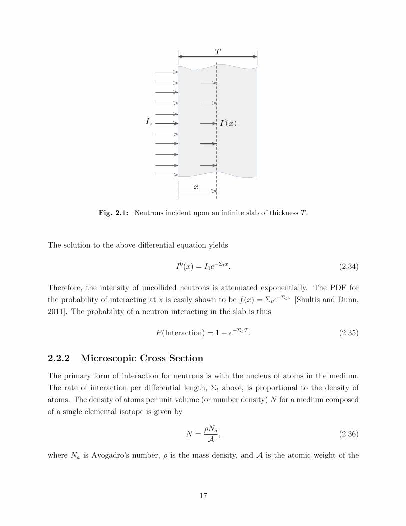
x
T
I 0 I 0( )x
Fig. 2.1: Neutrons incident upon an infinite slab of thickness T .
The solution to the above differential equation yields
I0(x) = I0e−Σtx. (2.34)
Therefore, the intensity of uncollided neutrons is attenuated exponentially. The PDF for
the probability of interacting at x is easily shown to be f(x) = Σte−Σt x [Shultis and Dunn,
2011]. The probability of a neutron interacting in the slab is thus
P (Interaction) = 1− e−Σt T . (2.35)
2.2.2 Microscopic Cross Section
The primary form of interaction for neutrons is with the nucleus of atoms in the medium.
The rate of interaction per differential length, Σt above, is proportional to the density of
atoms. The density of atoms per unit volume (or number density) N for a medium composed
of a single elemental isotope is given by
N =ρNa
A , (2.36)
where Na is Avogadro’s number, ρ is the mass density, and A is the atomic weight of the
17
element. With the above definition, the definition of Σt becomes
Σt ∝ N = σtN. (2.37)
The proportionality constant σt (cm2) is defined as the microscopic cross section and in-
dependent of N . The value of σt represents the total probability of interaction per unit
differential path length, normalized to a single target atom [Shultis and Faw, 2000]. Because
the values of σ are very small, the unit of barns is typically used, defined as 1b = 10−24cm2.
For an isotropic medium, the microscopic cross section is typically a function of the energy of
neutron and the particular isotope of nuclei present. In general, cross sections are relatively
larger at lower energies.
Cross sections are typically tabulated for each fundamental type of interaction, and the
occurrence of types of interactions are mutually exclusive events, therefore
σt =n∑i=1
σi, (2.38)
where σi is the cross section for the i-th of n types of interactions. The main interactions
for neutrons are absorption, fission, and elastic and inelastic scattering, which are discussed
thoroughly in [Shultis and Faw, 2000]. The terminology of absorption and capture can vary in
literature. Often absorption includes the fission and capture cross section, whereas capture
usually refers to (n, γ) reaction; the notation is target nucleus(incident particle, outgoing
particle)resulting nucleus, where the two nuclei are often omitted in a general case. For
clarity, herein neutron capture cross section is used to refer to any interaction in which a
neutron is absorbed without reemission of any neutrons (sometimes called a removal cross
section), i.e. σc = σn,γ + σn,p + σn,α + · · · .For a composite medium of isotopes, the total macroscopic cross section is given by
Σt =
niso∑j=1
Njσt, j, (2.39)
where the subscript j represents the j-th of niso isotopes.
2.2.3 Neutron Flux Density
An important property used to quantify a field of neutrons in a medium is the neutron
fluence. Consider a hypothetical sphere of volume ∆V with a field of neutrons traversing
the volume in any direction over some time t. The neutron fluence is defined as [Shultis and
18
Faw, 2000]
Φ = lim∆V→∞
[∑i si
∆V
], (2.40)
where si is the path length traversed through the volume by the i-th neutron track. In an
alternative definition, the neutron fluence (units of cm−2) is the number of particles that
have traversed a sphere of differential cross-sectional area, at a point. The neutron flux
density (abbreviated as flux) is the time-derivative of the fluence, i.e.,
φ =dΦ(t)
dt(2.41)
which is constant in time for steady-state applications. In general, the steady-state flux is a
function of neutron energy, direction, and position; respectively, φ = φ(E,Ω, ~r). The scalar
flux is the angular integrated flux, i.e., φ(E,~r), and in many detection application cases
the energy dependence is also integrated out. The flux can be defined alternatively as the
product of the neutron density per volume and the neutron speed. The flux is referring to
the scalar flux throughout this work.
The utility of the neutron flux is to directly calculate the reaction rate density using the
macroscopic cross section. The reaction rate density is the average number of interactions
occurring per unit volume, per unit time. Using the definition of flux as the differential
total path length traversed by all neutrons at a point, per unit time, and the macroscopic
cross section Σt as the differential probability of interaction per unit length, the reaction
rate density is
R(~r) = Σt(~r)φ(~r). (2.42)
Another useful parameter is the neutron current. The neutron current is the first angular
moment of the directionally dependent neutron flux. The current is useful because it provides
a measure of the net number of particles per unit area entering a surface.
2.2.4 Effective Neutron Multiplication Factor
In a system in which fission is present, the criticality of the system can be quantified by the
effective neutron multiplication factor, keff . Here, fission is referring to the process of an
unstable nucleus decomposing into two or more fragments. Fission can occur spontaneously
from unstable isotopes (e.g. 240Pu), or it can be induced by an incident neutron. When fission
occurs, multiple neutrons can be released. Thus, induced fission allowing for a self-sustaining
chains of neutron reactions to occur. Such a system is said to be critical. Quantifying the
sustainability of the population neutrons in a system is the value of keff defined as [Shultis
19
and Faw, 2008]
keff =# neutrons produced from fission in one generation
# of neutrons removed from the system in preceding generation. (2.43)
The value of keff is a product of the material properties and geometry of the system. A
system which produces a value of keff of unity is critical. In a critical system, the fission
process allows for the population of neutrons to remain constant in time. If keff > 1, then
the system is said to be supercritical. If keff < 1, the system is subcritical.
2.2.5 Neutrons Released per Fission ν
Typically, when fission occurs, one or more neutrons of varying energy are released from
the excessively energetic fission products, effectively instantaneously. The number of free
neutrons produced per fission, ν, is a vital parameter in modeling systems in which fission
occurs. In this work, ν is used to refer to the mean number of neutrons produced from induced
fission only, as it is the main interest. It is also noted that typically ν is divided into prompt
(induced fission) and delayed (fission fragments releasing neutrons through radioactive decay
at a later time) components. For this work, ν is referring to the sum of the prompt and
delayed neutrons, i.e., the total number of neutrons released per fission.
The parameter ν is formally a discrete random variable. The distribution of ν is de-
pendent upon the energy of incident neutron (i.e., ν = ν(E)) and the isotope of the target
nucleus. The distribution of ν(E) at an energy E is in general binomial, but it is known
to be well-approximated by shifted Gaussian distributions [X-5 Monte Carlo Team, 2003].
Typically, the mean of the distribution, ν , and variance σ2 are used to quantify unique dis-
tributions for each energy and isotope. Typical values of ν range from 1-4 for fissile isotopes,
generally increasing with the energy the of incident neutron.
For Monte Carlo simulations that investigate criticality, only sampling of ν(E) is needed
to properly recreate average macroscopic quantities (such as tallies or the neutron multi-
plication factor keff ) [X-5 Monte Carlo Team, 2003]. This is due to the large number of
neutrons present in the system. To sample ν , such criticality simulations typically sample
the integer values that bracket ν(E), such that the mean of the sampled values is ν(E). For
subcritical simulations, the distribution of ν(E) must be more accurately sampled. The typ-
ical sampling method is to sample integer values of ν(E) based on a Gaussian distribution
that properly identifies the distribution of ν(E) for a particular isotope and energy. The
Gaussian distribution has ν(E) as a mean at each energy E, but the value of the variance is
typically a constant for each isotope.
20

2.3 Monte Carlo Transport Code
2.3.1 The Monte Carlo Method and MCNP
The Monte Carlo method is a stochastic method, which can be used estimate average values
of physical parameters by simulating realistic behavior of the system of interest. In short, the
Monte Carlo method is to generate a large number of simulated trials (known as histories),
and then look at the average behavior of the histories. For radiation transport, a history
consists of creating and tracking a particle through a medium, using appropriate radiation
physics, until the particle terminates through leakage or absorption. The simulation uses
appropriate probability distributions (based on nuclear data) to simulate interactions and
trajectories of particles. Tallies are used to estimate some aspect of the radiation field.
Tallies are an estimate of the mean of some random variable (e.g. the neutron fluence).
A tally is estimated by taking the average of the contributions to some physical feature of
the neutron field of all particle histories. The statistical error associated with tallies is also
estimated, typically using the sample standard deviation of the tally of interest. The theory
behind the Monte Carlo method is discussed in detail in literature [Shultis and Dunn, 2011].
The majority of raw data in this work are generated from the Monte Carlo N-Particle
(MCNP) code (primarily version 5.1.51). The MCNP code is a general-purpose, fully 3-
dimensional transport code that allows for simulations of coupled neutron, photon, and
charge particle phenomena [X-5 Monte Carlo Team, 2003]. The code contains tabulated
nuclear data for all isotopes of interest. MCNP performs simulations by interpreting user-
created text input files which specify geometry, material properties, and physics and simula-
tion parameters. MCNP uses a Monte Carlo method that is continuous in phase space, i.e.,
particle tracks are continuous in energy, direction, and location. Tallies allow estimates of
the neutron flux, current, and reaction rate densities, as well as their respective statistical
uncertainties. MCNP6 is capable of accurate estimation of charge deposition by charge par-
ticles in a radiation detector. Along with the uncertainty in tallies, MCNP performs a series
of ten statistical tests to determine the statistical validity and convergence of tally scores
and uncertainties. A full description of specific features of the code, as well as an overview
of Monte Carlo modeling of radiation physics, can be found in the manual [X-5 Monte Carlo
Team, 2003].
2.3.2 Non-Analog Variance Reduction in MCNP
Various non-analog simulation techniques are available to reduce the uncertainty in tallies
and to help pass the ten statistical tests without increasing the number of particle histories.
21
Several of these techniques used in design of the spectrometer to improve the efficiency of
simulations are discussed here. There are other analog truncation methods (such as particle
energy cut-offs) implemented implicitly, which are straight forward and discussed in Shultis
and Faw [2004].
The basic goal of variance reduction techniques is to decrease the uncertainty in a tally,
without increasing the number of histories. Additionally, variance reduction helps to improve
convergence of the problem and pass the ten statistical tests provided by MCNP. Passing
these tests provides assurance that the central limit theorem (see Shultis and Dunn [2011])
is valid for the tally of interest. When the central theorem is valid, the tally has a Gaussian
distribution with a mean and standard deviation given by the tally’s reported value and
sample standard deviation. To ensure that variance reduction techniques do not introduce
bias into the mean, the techniques must also operate on the so-called weight, or importance,
of the particle history. When tallies sum a property of a particle during a history, the partic-
ular properties are multiplied by the corresponding weight of the particle in the summation.
This prevents biasing of results [X-5 Monte Carlo Team, 2003].
Implicit Capture
Implicit capture is a feature that is turned on by default in MCNP5. When a particle
undergoes an absorption event, rather than terminating the history, the history is continued
with the particle’s weight reduced by a factor equal to the conditional probability of non-
absorption (1− σc/σt). This feature cannot be used in charge deposition simulations, where
the exact location of absorption is of importance [X-5 Monte Carlo Team, 2003].
Cell-Based Splitting
MCNP geometry is divided into contiguous geometric regions known as cells, which have
an importance assigned to them. Non-void cells that are closer to a tally are generally
considered more important to the problem. The importance in these cells can be increased
as the position gets closer to tallies of interest as a form of variance reduction.
If a particle crosses from one cell to another with higher importance, the particle is
divided into n particles with the same velocity as the original particle; the weight of each
new particle is the original particle weight reduced by a factor of 1/n. The factor n is the
ratio of the importance of the cell the particle is entering to the importance of the cell the
particle is exiting. A form of uniform random sampling is performed to produce an integer
number of new histories. If a particle enters a cell with lower importance than its current
cell, then the history is either terminated with a probability proportional to the ratio of the
22
importances, or it is continued with the weight increased by a factor equal to the inverse of
the ratio. It is noted that the ratio is independent of the weight of the particle traversing
the surface; it is only dependent upon the two cell importances.
Cell splitting can cause a bias in results by truncating the model if the splitting being
performed is too extreme. As a good rule of thumb, it is ideal to have the number of particles
in each cell to be approximately equal [X-5 Monte Carlo Team, 2003]. It is also important
that adjacent cells should not increase or decrease in importance by more than a factor of 4.
Russian Roulette
Similar to splitting is the Russian roulette technique. Russian roulette is performed to
terminate histories that are very unlikely to contribute to a tally, based on the weight of
the particle. When the weight of a particle drops below a certain threshold value during a
history (the weight is reduced by other variance reduction techniques), the history is either
terminated or continued. The probability of terminating the history is inversely proportional
to weight of the particle. If the history continues, then it is continued with a weight increased
by a factor equal to the inverse of the weight.
Directional Source Biasing
Biasing the emission direction of created source particles can produce very effective results
in MCNP. This is typically useful for isotropic point sources. To illustrate the technique,
consider a point source and a detector in a void. Then, only neutrons traveling directly at
the detector volume would be detected. The remaining histories would terminate without
interacting or contributing to the tally. To improve efficiency, the simulation should only
sample source particles with directions that will contribute to the tally. Assuming some
reference direction is specified, source biasing is typically performed based on the cosine
of the polar angle between the reference and particle emission directions. Emission over
the azimuthal angle as measured from the reference direction is assumed to be isotropic.
To prevent biasing, the weight of each emitted source particle is reduced by the fractional
subtended solid angle. If particles are only emitted between polar angles with cosines between
µmin and µmax, the weights are given by (assuming all particles would otherwise start with
a weight of 1) (µmax−µmin)/2. In other cases, source particles in a particular direction may
be required to back-scatter from a distant wall before reaching the tally. Performing source
biasing in this case introduces modeling truncation error, essentially replacing that region of
the problem with a void. This truncation error may be negligible in many cases to the mean,
but the loss of those rare events will significantly improve the convergence of the problem.
23

Chapter 3
Review of Neutron Spectrometry
This chapter reviews current and previous methods for neutron spectrometry. Only portable,
relatively quick discriminating spectrometer designs are of interest, so methods (e.g. time of
flight) used for discerning neutron energies for precise needs are not discussed, but can be
found in the literature [Tsoulfanidis, 1995; Brooks and Klein, 2002]. The general unfolding
problem and solution methods are developed, then designs utilizing this method, as well as
others, are discussed.
3.1 The Unfolding Problem
3.1.1 The Unfolding Equation
The general approach of spectrum unfolding is to identify a source spectrum from a series of
measured responses that represent different unique energy ranges. The general relation for
an unfolding problem for an energy spectrum can be stated as [Tsoulfanidis, 1995]
M(E) =
∫ ∞0
R(E,E ′)S(E ′) dE ′, (3.1)
where M(E) is the measured distribution function with respect to energy E, S(E ′) is the
distribution of the number of source particles emitted as a function of E ′, and R(E,E ′) is a
kernel that represents the probability an emitted source neutron at energy E ′ is measured at
energy E and is known as the response function. Often response functions are adjusted to
account for dose. The general term dose refers to some measure of the correlation between
biological effect and an observed response based on deposited energy and type of radiation,
as a function of incident particle energy. Although the focus of this work is in identifying the
type of neutron sources based on energy spectrum, most spectrometry designs and research
24
focus on estimating radiation dose. The primary difference between unfolding a dose and an
energy spectrum is in the definition of the response functions.
Eq. (3.1) is a Fredholm integral equation of the first kind [Twomey, 1963]. The general
method is to solve for S(E ′), assuming the response function is known via measurement or
simulations, by inverting the measured responses M(E). The function M(E) is generally
not continuous. Rather, discrete values are measured which represent the energy-integrated
response over a certain energy range, i.e.,
M(E) ≈Mi, Ei < E < Ei+1, (3.2)
where
Mi =
∫ Ei+1
Ei
M(E) dE, i = 1, 2, . . . , Ndet. (3.3)
Here Ndet is the number of unique energy-dependent detector measurements. The response
function R(E,E ′) can be determined by experiment or simulation.
The inverse problem of Eq. (3.1) can be discretized by application of some appropriate
numerical quadrature scheme, i.e.,
∞∫0
f(E ′) dE ′ 'Nerg∑j=1
wjf(E ′j), (3.4)
where f(E ′) is any continuous function of E ′, and Nerg is the number of discrete energy
groups of the solution. Application of this numerical quadrature to the right hand side
of Eq. (3.1), with the substitution of Eq. (3.3) for M(E), yields the set of linear algebra
equations
Mi =
Nerg∑j=1
RijSj, i = 1, 2, . . . , Ndet, (3.5)
where R(E,E ′) has been discretized to form a response matrix with elements
Rij = wj
∫ Ei+1
Ei
R(E,Ej) dE, j = 1, 2, . . . , Nerg and i = 1, 2, . . . , Ndet. (3.6)
The desired solution is the discretized source energy spectrum, i.e., Sj = S(Ej) for j =
1, 2, . . . , Nerg. Typically in neutron detection measurements, primarily only thermal neutrons
are detected directly because of higher absorption probabilities in detection materials at lower
energies. Higher energy neutrons are lowered to thermal energies for detection by adding
moderator to the system. Therefore, a unique detector-moderator arrangement is needed for
25
each value Mi, so generally the number of measurements is limited.
3.1.2 Regularizing the Set of Algebraic Equations
As neutron energies are typically continuous, inferring a neutron energy spectrum from a
limited number of detector measurements is a difficult problem. For continuous energy
sources, unfolding the discrete measured spectrum usually leads to an underdetermined
system of linear equations (i.e., Nerg > Ndet). An underdetermined problem is one in which
there are more unknowns than equations, which leads to an infinite number of solutions or
no solution. An underdetermined set of equations is an ill-posed problem mathematically.
In the case of unfolding, there are typically an infinite number of solutions so that some a
priori information must be input into the solution method. The additional information is
applied to achieve a unique and realistic (e.g., non-negative) solution.
The general approach of solving an underdetermined system is to regularize the set of
equations. Regularization is a process that introduces assumptions about the solution that
provide additional equations. After regularization, the total number of equations equals the
number of variables, leading to a solvable set of linear equations. The general approach of
regularization is to minimize the expression [Press et al., 1992]
A[S] + λB[S], (3.7)
where S is a column vector containing the desired solution spectrum Sj : j = 1, 2, . . . , Nerg,A[S] is a positive functional that measures how well the solution S satisfies Eq. (3.5), and
B[S] is a positive functional that measures how well S satisfies some a priori information
applied to regularize the system. Here, the weighting factor λ is a parameter of the solution.
For increasing values of λ, between 0 and ∞, the solution S(λ) provides a trade-off of the
minimization of A and B. The choice of λ is determined by the user. Although the choice
of λ is subjective, a common choice is to determine λ such that A[S] ensures S agrees with
the values of Mi within one standard deviation, for all i [Press et al., 1992].
The forms of A and B vary with solution method, in some cases leading to non-linear
equations [Press et al., 1992]. A common choice for A is a χ2 goodness-of-fit statistic.
The functional B provides a numerical measure of the smoothness of each of the Sj(E) or
their derivatives. For linear regularization, B = STHS, where H is a smoothing matrix.
The smoothing matrix is chosen such that the functional form of the Sj is assumed (e.g.,
quadratic or cubic). The matrix H applies finite differencing to the derivatives of the Sj
such that the minimization of B produces the desired shape of the solution. The specific
form of smoothing matrices, as well as higher-order and non-linear regularization methods,
26
can be found in [Press et al., 1992].
3.2 Solution Methods
Many methods and computer codes have been developed to regularize equations and un-
fold the source energy spectrum. Often the methods of constraining the solution are semi-
empirical and subjective, requiring the user to have substantial experience. Smoothing of
data after unfolding is often applied [Tsoulfanidis, 1995]. Historically, a constrained linear-
least-squares method was utilized, but suffered from numerical instability [Twomey, 1963].
The linear-least-squares method is a zeroth-order regularization method, i.e., there is no
constraint on the smoothness of the derivatives of the solution [Press et al., 1992]. Itera-
tive solution methods are far more common and have been used and studied extensively.
The class of iterative solution methods involved in underdetermined problems are often nu-
merically instable and computationally demanding (relative to an on-board processor for
real time spectrometry). Also, an estimated solution from the user is typically required,
so the user must have a good estimate of what the source is to begin with. Two of the
more common commercial codes which modern codes have adapted and improved upon are
SPUNIT [Brackenbush, 1983] and BUNKI [Miller, 1993]. Neural-networking and genetic
based algorithm codes have been developed more recently to unfold spectra that have the
potential to be more efficient and portable [Fayegh, 1993; Mukherjee, 2002]. To simplify
the process of unfolding, recently a more user-friendly rendition of SPUNIT has been devel-
oped by Vega-Carrillo et al. [2012], as well as a user interface compilation of unfolding codes
by Sweezy et al. [2002].
Although smoothing of calculated data is generally not desired, it has been shown in
application to improve unfolding results [Tsoulfanidis, 1995]. Data smoothing attempts to
make the spectrum more continuous and physically realistic based on an expected solution
and behavior of the data curve. The general approach to smoothing is to estimate the
expected average behavior of the true spectrum, at some point in the unfolded spectrum,
based on the behavior of surrounding energy points and fitting some form of a polynomial
between those points. This is repeated in a pointwise manner, essentially removing distortion
from statistical noise. A brief overview of smoothing methods can be found in [Grissom and
Koehler, 1971].
27
3.3 Neutron Spectrometer Designs
In this section, neutron spectrometer designs are divided into two categories. The first set of
designs are those that use a single energy-averaged measurement to estimate the response or
dose from a multiple-energy neutron field. The second are those which use multiple energy-
dependent observations to calculate the response or dose, typically through unfolding. The
latter are more comparable in application to the design in this work, while the former is
discussed briefly because it is the most commonplace use of neutron spectrometry in study
and application [Thomas and Alevra, 2002].
3.3.1 Single Detector Response Systems
Detection systems used for estimating a dose from a variable energy neutron field via a sin-
gle detector response are the most commonplace application of energy-dependent neutron
data Brooks and Klein [2002]. The Bonner sphere [ICRU, 2001] is the most commonly used
device to estimate neutron dose. The basic design of a Bonner sphere is a thermal neutron de-
tector surrounded by a sphere of polyethylene moderator. The encapsulated detector demon-
strates a similar energy-dependent response function to that of a human phantom [ICRU,
2001]. Thus, a single measurement from a Bonner sphere is directly comparable to the ex-
pected dose experienced by a human in the same neutron field. Many models of spherical
and cylindrical designs have been implemented since Bonner sphere was introduced in 1960,
as discussed by Thomas and Alevra [2002]. Modifications to the design over the last decade
have focused on reducing weight (e.g. the WENDI design [Olsher, 2000] and [Yoshida et al.,
2011]). For neutron dose measurements near high-energy particle accelerators, several recent
designs [Biju et al., 2012; McLean and Justus, 2012; Yoshida et al., 2011] utilize a heavy
metal, e.g. tungsten or zirconium, to convert very high energy neutrons (10 MeV–1 GeV)
into multiple neutrons at lower energies via (n, xn) reactions.
3.3.2 Multiple Detector Response Systems
The historical method of gathering energy dependent information about a neutron field is
through measurements from multiple Bonner spheres of differing diameters, first proposed
in Bramblett [1960]. The Bonner sphere spectrometry (BSS) system is based on taking
individual measurements with a thermal neutron detector surrounded by spheres of vary-
ing radius of polyethylene. The measurements are typically unfolded to estimate either
the energy spectrum or an energy-dependent dose. The number of measurements needed
to identify an energy spectrum correctly may vary, but usually a minimum of around six
28
measurements is needed [Thomas and Alevra, 2002]. Additionally, although each sphere is
primarily sensitive to a single range of neutron energies, there is overlap of response func-
tions in different energy ranges (i.e., multiple spheres demonstrate a measurable response
from a monoenergetic source) [Brooks and Klein, 2002]. This is the fundamental difficulty
in unfolding energy spectra from a BSS system. Overall, BSS systems are able to cover a
wider range of energies with a higher efficiency than most other systems, but the unfolded
spectrum has poor energy resolution [Thomas and Alevra, 2002]. A BSS system is not ideal
for identification of special nuclear material because of the requirement of individual device
measurements, large moderator weight, and poor resolution.
An alternative design that has been studied extensively is proton recoil spectrometers.
Proton recoil spectrometers are based on interactions of a neutron with a proton (in the form
of hydrogen within the detection volume), and the measurement of the kinetic energy of the
resulting recoil proton after the collision. As the proton is of similar mass as the neutron,
it can potentially absorb all of the kinetic energy of an interacting neutron. All the data
to determine the spectra can be obtained from a single measurement using a multichannel
analyzer [Flaska and Pozzi, 2007a], rather than the multiple individual measurements needed
with a BSS system. Organic scintillators are favorable for recoil spectrometers because they
allow discrimination of gamma and neutron signal through pulse-shape analysis of the time-
dependent detector output voltage [Brooks and Klein, 2002].
The application of recoil spectrometers for quick source identification is limited by their
relatively small energy range and low efficiency. Proton recoil spectrometers are typically
only effective within the range of 50 keV – 4 MeV [Brooks and Klein, 2002]. PRESCILA is a
current mixed detector design that is capable of unfolding dose estimates over a much wider
energy range [Olsher, 2004]. PRESCILA utilizes a proton recoil and cadmium coated thermal
neutron detector to measure fast, epithermal, and thermal neutrons simultaneously. The
device provides wide-range dose in a single measurement, but demonstrates large inaccuracies
in some energy ranges (as high as 300%) [Caruso et al., 2011].
For the specific application of source identification, a neutron scatter camera using recoil
spectrometers and time of flight measurements has been used to distinguish among different
neutron sources [Brennan et al., 2011]. The device utilizes 32 liquid scintillator sections where
proton recoils are measured and time of flight is coupled to scattering events to determine
the angle and energy of incident neutrons; the resulting spectra are then unfolded. The
device has been shown to identify individual sources correctly, but is not portable and the
required neutron population for identification is not discussed in the article.
A different method utilizing proton recoil which does not depend on energy unfolding has
been studied previously by Flaska and Pozzi [2007b]. The method utilizes a well-developed
29

method for discriminating gamma rays from neutrons based on the difference in the magni-
tude and shape of detector output pulse heights, relative to the pulse tails. In addition to
no unfolding, another favorable attribute of the method is the potential ability to identify
sources in the presence of shielding, as the pulse height shapes showed minimal change [Flaska
and Pozzi, 2007a]. Another advantage of this method is that it potentially will require far
fewer neutron counts than other methods. Experiments and simulations have been per-
formed, demonstrating proof of concept. The robustness and applicability of the method
have not been studied beyond identification of 252Cf, americium-beryllium, and americium-
lithium sources.
Some recent spectrometer designs have used multiple detectors encased in a single large
moderator. The appeal of this design is to obtain the efficient, wide-range energy measure-
ments of a BSS system in a single measurement. Having all the detectors in the moderator
and making the measurements simultaneously requires detectors that provide high efficiency
for minimal volume and perturb the neutron flux minimally. A design using three 3He po-
sition sensitive thermal neutron detectors in a sphere of polyethylene was built and tested
by Toyokawa et al. [1997]. The device was able to estimate dose over a wide energy range,
but it was not as accurate as BSS systems (typically underestimating at most energies), and
dose estimates were directionally dependent. A design similar in construction to that of this
work has been implemented which utilizes an array of pixelated detectors embedded in a
cylinder of HDPE by Caruso et al. [2011]. The pixelated detectors consist of a hexagonal
array of high-efficiency perforated neutron detectors [Shultis and McGregor, 2009]. The pix-
elated detectors allow radial information about the neutron field to be measured, making
spectrum unfolding more accurate and efficient. Unfolded dose estimates were able to match
dose curves to within 15% for several sources over a large energy range; these dose estimates
are more accurate than designs currently available utilizing a single detection measurement.
30
Chapter 4
Simulations of a Neutron Source
Identification Spectrometer
The focus of this chapter is the optimization and design of a new type of neutron spectrom-
eter [Cooper et al., 2011]. Although it is referred to as a spectrometer, the device discussed
herein identifies the type of a neutron source based on measurements which implicitly de-
pend on the neutron energy spectrum. The actual energy spectrum of a source is never
explicitly determined from the detector measurements. However, any unfolding techniques
used by other spectrometers could, in principle, be applied to measurements made with this
spectrometer.
First, the methodology for the source identification technique used by the spectrometer
being studied is presented. Then, the geometry and the MCNP model is discussed. After
that, methodology and results for optimizing the geometry of the system are given. A method
utilizing a neutron shadow shield to correct measurements for room-scattered neutrons is also
investigated. Finally, closing remarks and suggestions for future design work are given.
4.1 Methodology
4.1.1 Overview
As discussed in Chapter 1, the spectrometer consists of cylindrical sections of HDPE with
high efficiency thermal neutron detectors contained within. A sheet of Cd is placed behind
each detector to reduce the effect of backscattered neutrons. A large library of unique
spectrometer responses, known as templates, is pre-generated. On page 33, Fig. 4.1 plots
several example spectrometer responses for different types of bare neutron sources that were
simulated with the MCNP5 model discussed later in Section 4.2.1; the detector responses
31
are given as counts per neutron incident upon the front of the spectrometer. The detector
responses are then normalized by dividing the response at each detector position by the
response in the second detector position, as demonstrated in the figure. The normalization
removes dependence of the detector responses on the intensity of incident neutrons. Each
set of normalized detector responses forms a template. As discussed in Chapter 1, each
template is unique to an incident neutron energy spectra. Ideally, templates are generated
for all possible neutron sources for the particular spectrometry application. To identify a
neutron source, a measured spectrum of detector counts (normalized to the second detector
position) is compared against each template in the library. The template which is most
similar to the measured spectra identifies the most likely neutron neutron source.
Although there are relatively few neutron sources (e.g., AmBe, PuBe, and spontaneous
fission sources) compared to the number of different radioisotopes, the neutron spectra emit-
ted by these sources can be many as a consequence of inert material surrounding the source
material perturbing the original source spectrum. The effect of shielding materials must be
accounted for in application by including templates for different source and shielding com-
binations. The required robustness of templates to account for the effect of shielding on
spectrometer responses is not considered in this work.
4.1.2 Source Identification Based on a FOM
To determine the most likely source for a set of observed detector measurements (herein
referred to as a detector spectrum), the individual measurements at each detector position
are compared to corresponding reference values for different sources. Comparisons are made
using an approximate χ2 statistic as a figure of merit (FOM). As discussed above, the
reference spectra are unique to each neutron source1. For a particular measured spectrum,
a FOM is calculated for each template. The template that produces the lowest FOM is
identified as the most likely source.
For a spectrometer with Ndet detectors irradiated by neutrons with some unknown energy
distribution, a set of measurements Ci : i = 1, 2, . . . , Ndet is observed. Here, Ci is the
counts recorded by the detector in the i-th position (position indices are indexed with 1
being nearest the source, and Ndet being farthest from the source). To remove dependence
in these values on the strength of the neutron source under investigation, the set of counts
is normalized such that one of the detector’s counts is unity. Then, the logarithm of each
normalized value is taken to simplify error propagation calculations later on. The set of
1Although only bare neutron sources are considered in this work, templates could account for factors suchas shielding. Thus, a particular energy distribution of incident neutrons is all that is specified by a unique“neutron source” in this chapter.
32
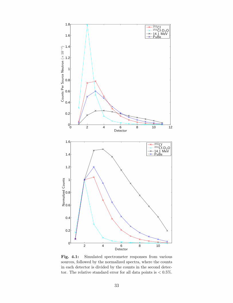
0 2 4 6 8 10 120
0.2
0.4
0.6
0.8
1
1.2
1.4
1.6
1.8
Counts
Per
SourceNeutron(×
10−3)
Detector
252Cf252Cf-D2O14.1 MeVPuBe
2 4 6 8 100
0.2
0.4
0.6
0.8
1
1.2
1.4
1.6
Norm
alized
Counts
Detector
252Cf252Cf-D2O14.1 MeVPuBe
Fig. 4.1: Simulated spectrometer responses from varioussources, followed by the normalized spectra, where the countsin each detector is divided by the counts in the second detec-tor. The relative standard error for all data points is < 0.5%.
33
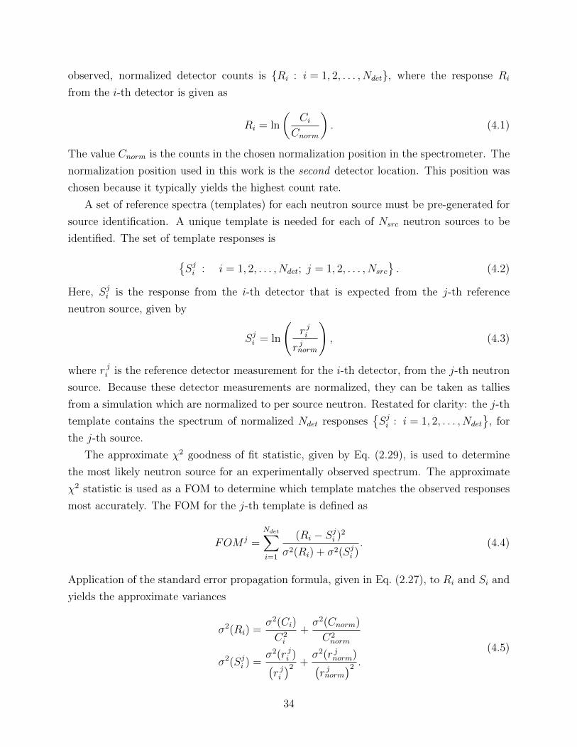
observed, normalized detector counts is Ri : i = 1, 2, . . . , Ndet, where the response Ri
from the i-th detector is given as
Ri = ln
(Ci
Cnorm
). (4.1)
The value Cnorm is the counts in the chosen normalization position in the spectrometer. The
normalization position used in this work is the second detector location. This position was
chosen because it typically yields the highest count rate.
A set of reference spectra (templates) for each neutron source must be pre-generated for
source identification. A unique template is needed for each of Nsrc neutron sources to be
identified. The set of template responses is
Sji : i = 1, 2, . . . , Ndet; j = 1, 2, . . . , Nsrc
. (4.2)
Here, Sji is the response from the i-th detector that is expected from the j-th reference
neutron source, given by
Sji = ln
(r jir jnorm
), (4.3)
where r ji is the reference detector measurement for the i-th detector, from the j-th neutron
source. Because these detector measurements are normalized, they can be taken as tallies
from a simulation which are normalized to per source neutron. Restated for clarity: the j-th
template contains the spectrum of normalized Ndet responsesSji : i = 1, 2, . . . , Ndet
, for
the j-th source.
The approximate χ2 goodness of fit statistic, given by Eq. (2.29), is used to determine
the most likely neutron source for an experimentally observed spectrum. The approximate
χ2 statistic is used as a FOM to determine which template matches the observed responses
most accurately. The FOM for the j-th template is defined as
FOM j =
Ndet∑i=1
(Ri − Sji )2
σ2(Ri) + σ2(Sji ). (4.4)
Application of the standard error propagation formula, given in Eq. (2.27), to Ri and Si and
yields the approximate variances
σ2(Ri) =σ2(Ci)
C2i
+σ2(Cnorm)
C2norm
σ2(Sji ) =σ2(r ji )(r ji)2 +
σ2(r jnorm)(r jnorm
)2 .
(4.5)
34
Because the distribution of observed counts in a detector usually follows a Poisson dis-
tribution, as described in Section 2.1.5, the observed counts is used as the mean of the
Poisson distribution, and the uncertainty for a particular observed measurement is taken as
σ2(Ci) = Ci. When this result is substituted into Eq. (4.5), the uncertainties above reduce
to
σ2(Ri) =1
Ci+
1
Cnorm
σ2(S ji ) =
σ2(r ji )(r ji)2 +
σ2(r jnorm)(r jnorm
)2 .(4.6)
The lower the value of FOM j, relative to the FOM of other sources, the more accurately
the j-th template spectrum matches the observed spectrum. Thus, the FOM corresponding
to the template which is most likely the source is given by
FOMmin = min FOM j : j = 1, 2, . . . , Ntemp, (4.7)
where Ntemp is the number of templates and FOMmin is the minimum of the set of FOM
values. It is noted that typically a system is optimized by increasing the FOM, unlike here,
where lower values are preferred. The FOM nomenclature was chosen to prevent confusion
with χ2 hypothesis testing (as well as other χ2 values in this work) and to emphasize that
the FOM statistic is approximate and not necessarily sampled from a χ2 distribution.
The random variables, from which the values FOM j are sampled, follow distributions
that are generally unknown. As a result, the source corresponding to FOM(0) is not nec-
essarily the correct source (particularly when there are insufficient counts in the detectors).
To give a measure of how uncertain a source identification is, an approximate standard devi-
ation of the FOM values is used. From Eq. (2.30), the standard deviation in a FOM value
is approximated as
σ(FOM) = 2√FOM. (4.8)
It is of note that Eq. (4.8) is not the true standard deviation; it is an approximation based
on the standard error propagation formula, which predicts the behavior of FOM values from
uncertainty in the counting and template measurements. The error propagation formula uses
a first order Taylor series approximation, which can be very inaccurate for some functions.
It is also noted that because FOM ∈ [0,∞), the confidence intervals are asymmetrical. In
general, standard Gaussian confidence intervals are not applicable here.
The degrees of freedom of the FOM value is Ndet − 1. The reduction by one degree is
because the detector spectra are normalized to the counts in one detector; the values Rnorm
and Snorm will always be 1, and thus that detector never contributes to the FOM .
35
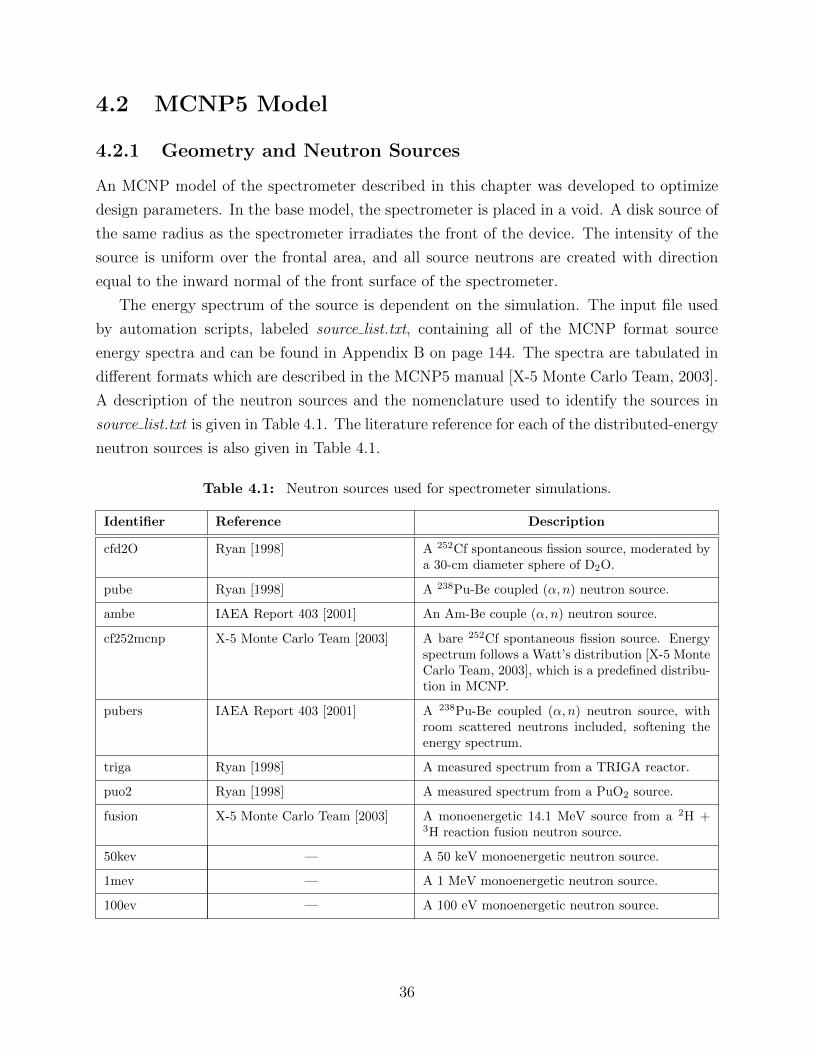
4.2 MCNP5 Model
4.2.1 Geometry and Neutron Sources
An MCNP model of the spectrometer described in this chapter was developed to optimize
design parameters. In the base model, the spectrometer is placed in a void. A disk source of
the same radius as the spectrometer irradiates the front of the device. The intensity of the
source is uniform over the frontal area, and all source neutrons are created with direction
equal to the inward normal of the front surface of the spectrometer.
The energy spectrum of the source is dependent on the simulation. The input file used
by automation scripts, labeled source list.txt, containing all of the MCNP format source
energy spectra and can be found in Appendix B on page 144. The spectra are tabulated in
different formats which are described in the MCNP5 manual [X-5 Monte Carlo Team, 2003].
A description of the neutron sources and the nomenclature used to identify the sources in
source list.txt is given in Table 4.1. The literature reference for each of the distributed-energy
neutron sources is also given in Table 4.1.
Table 4.1: Neutron sources used for spectrometer simulations.
Identifier Reference Description
cfd2O Ryan [1998] A 252Cf spontaneous fission source, moderated bya 30-cm diameter sphere of D2O.
pube Ryan [1998] A 238Pu-Be coupled (α, n) neutron source.
ambe IAEA Report 403 [2001] An Am-Be couple (α, n) neutron source.
cf252mcnp X-5 Monte Carlo Team [2003] A bare 252Cf spontaneous fission source. Energyspectrum follows a Watt’s distribution [X-5 MonteCarlo Team, 2003], which is a predefined distribu-tion in MCNP.
pubers IAEA Report 403 [2001] A 238Pu-Be coupled (α, n) neutron source, withroom scattered neutrons included, softening theenergy spectrum.
triga Ryan [1998] A measured spectrum from a TRIGA reactor.
puo2 Ryan [1998] A measured spectrum from a PuO2 source.
fusion X-5 Monte Carlo Team [2003] A monoenergetic 14.1 MeV source from a 2H +3H reaction fusion neutron source.
50kev — A 50 keV monoenergetic neutron source.
1mev — A 1 MeV monoenergetic neutron source.
100ev — A 100 eV monoenergetic neutron source.
36
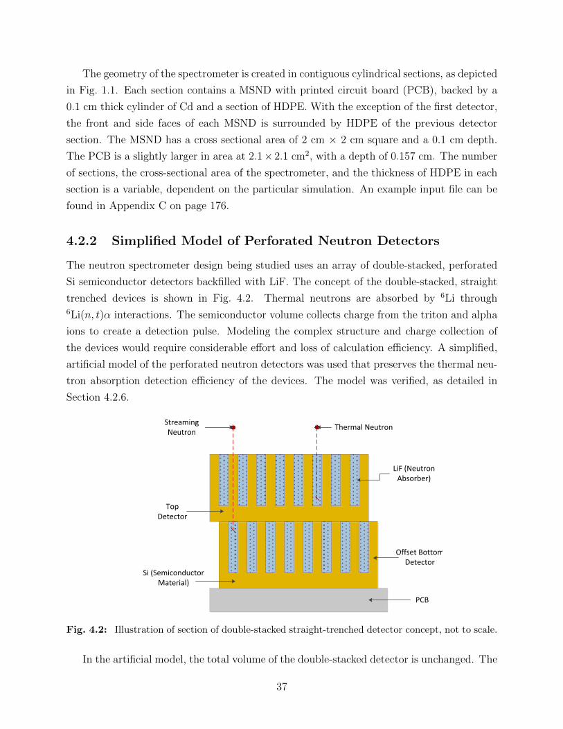
The geometry of the spectrometer is created in contiguous cylindrical sections, as depicted
in Fig. 1.1. Each section contains a MSND with printed circuit board (PCB), backed by a
0.1 cm thick cylinder of Cd and a section of HDPE. With the exception of the first detector,
the front and side faces of each MSND is surrounded by HDPE of the previous detector
section. The MSND has a cross sectional area of 2 cm × 2 cm square and a 0.1 cm depth.
The PCB is a slightly larger in area at 2.1× 2.1 cm2, with a depth of 0.157 cm. The number
of sections, the cross-sectional area of the spectrometer, and the thickness of HDPE in each
section is a variable, dependent on the particular simulation. An example input file can be
found in Appendix C on page 176.
4.2.2 Simplified Model of Perforated Neutron Detectors
The neutron spectrometer design being studied uses an array of double-stacked, perforated
Si semiconductor detectors backfilled with LiF. The concept of the double-stacked, straight
trenched devices is shown in Fig. 4.2. Thermal neutrons are absorbed by 6Li through6Li(n, t)α interactions. The semiconductor volume collects charge from the triton and alpha
ions to create a detection pulse. Modeling the complex structure and charge collection of
the devices would require considerable effort and loss of calculation efficiency. A simplified,
artificial model of the perforated neutron detectors was used that preserves the thermal neu-
tron absorption detection efficiency of the devices. The model was verified, as detailed in
Section 4.2.6.
Heading
Offset Bottom Detector
LiF (Neutron Absorber)
Top Detector
Si (Semiconductor Material)
PCB
Thermal NeutronStreaming Neutron
Fig. 4.2: Illustration of section of double-stacked straight-trenched detector concept, not to scale.
In the artificial model, the total volume of the double-stacked detector is unchanged. The
37
detector volume is modeled in MCNP as 6Li at a reduced density that produces the same
probability of absorbing a thermal neutron as the thermal neutron absorption detection effi-
ciency of the device. Here, detection efficiency is defined as the probability of an absorption
event depositing enough charge to be an observable event. In the artificial model, the Si
and F are ignored as they have minimal effect on thermal neutron interactions relative to
the high absorption in 6Li. Although Si and F have larger interaction coefficients at higher
energies, relative to the moderator they have a minimal effect.
Because interactions besides absorption are negligible in 6Li at thermal energies, expo-
nential attenuation of neutrons via the absorption cross section can be assumed. For a
normally-incident beam of thermal neutrons, the probability of neutron absorption in a slab
of thickness T of 6Li is
εthermal = 1− exp
[−ρ(6Li)Na
A(6Li)σn,t(
6Li)T
], (4.9)
where Na is Avagadro’s constant, σn,t(6Li) is the thermal-averaged cross section, ρ(6Li) is
the effective density, and A(6Li) is the atomic weight of 6Li. Solving for ρ(6Li) required to
achieve a given efficiency ε produces
ρ(6Li) = − ln(1− ε)A(6Li)
Naσn,t(6Li)T. (4.10)
The thermal (2200 m s−1) cross section σn,t(6Li) is 940 b [Chart of the Nuclides, 16th Ed.].
The (n, t) cross section is assumed to have a 1/√E behavior with respect to incident neutron
energy E over the thermal energy range. With this assumption, and the assumption that
the thermal neutrons are in equilibrium at room temperature, the thermal-averaged cross
section becomes [Stacey, 2007]
σn,t(6Li) =
√π
2σn,t(
6Li) = 833 b. (4.11)
The detection region for each module of the spectrometer consists of a 2 × 2 array of 1
cm2 devices, with a total detector thickness of 0.1 cm. The region was modeled in MCNP
as a 2 cm × 2 cm, 0.1 cm thick rectangular box (a detector volume, Vd, of 0.4 cm3). The
intrinsic detection of efficiency of the devices was taken as 50%; this is an achievable detection
efficiency of a dual-stacked device with this thickness [Shultis and McGregor, 2009]. Although
this may not be the actual efficiency of the devices, it will not affect the optimization results
of the spectrometer. As long as the efficiency of the devices is uniform, the results will not
be affected because a different detection efficiency can be compensated for by increasing the
38
total count time. The effective density of 6Li given by Eq. (4.10) for a rectangular box that
is 0.1 cm thick with a 4 cm2 face was found to be ρ(6Li) = 0.08353 g cm−3.
4.2.3 Detector Response in MCNP5
The FM card (text input parameters in MCNP are referred to as cards) in MCNP5 was
used to convert the F4 cell-volume averaged flux tally to counts per source neutron [X-5
Monte Carlo Team, 2003]. The FM card was used with 2 options: the reaction id, rid, for
the interaction of interest and the constant multiplier C. The FM card with these options
modifies an F4 response to be
R (counts per source neut.) = C
∫ ∞0
σn,t(E)Φ(E) dx, (4.12)
where R is the simulated detector response and Φ(E) is the average fluence over the detector
volume Vd per source particle (the result of the F4 tally). For the detection volume discussed
in Section 4.2.2, C is given by
C = Vdρ(6Li)Na
A(6Li)× 10−24. (4.13)
The rid for the (n, t) reaction is 105, and for ε = 50%, Eq. (4.13) reduces to C = 0.0083216Vd.
For the particular case of the detectors modeled here with Vd = 0.4 cm3 for each artificial
double-stacked detector volume, the value is C = 0.0033286. It should be noted that the FM
card in this case is specific to a material card, but also specific to the volume of the cells
of the F4 tally. The use of the FM card in this manner determines the expectation value
of a particular reaction rate in a volume by integrating the product of the energy-depedent
neutron flux and cross section of the reaction over all neutron energies. Thus, the result of
this tally is approximating the number of neutrons, per source particle, that would deposit
at least 300 keV of energy in an explicit model of a detector.
The tallies for the response from each detectors are grouped into a single input tally
card. MCNP then multiplies the individual responses for the F4 tallies by the necessary
multiplier. The detector volume cells in the model begin at cell 10, increasing by 10 with
increasing detector depth. For example, the tally specification for a spectrometer with 5
detectors would be
F4:N 10 20 30 40 50
FM4 0.0033286 2 105
where 2 is the detection material number and 105 is the rid. The TF input parameter was then
39
used to modify how MCNP checks statistical convergence. The deepest detector position for
any particular spectrometer is the most likely tally to have poor statistics because particle
histories are less likely to reach it. As an example input, to get the statistical tests for the
last cell for the above F4 tally, the TF4 input would be
TF4 5 7j
where 5 indicates to use the fifth entry on the tally card F4 for statistical convergence tests,
and 7j simply skips the remaining optional inputs for the card.
4.2.4 Boron in Circuit Boards
The PCBs on the back of perforated semiconductor detectors used in the spectrometer are
placed on contain neutron absorbers, namely B and Br used for flame retardant purposes, as
well as other materials such as Cu and C. The thermal neutron absorption cross section of10B is large (3,840 b [Chart of the Nuclides, 16th Ed.]). The concentration of these materials
in PCBs is proprietary to manufacturers, and thus generally unknown.
To include the amount of 10B in the models, an equivalent atom density of 10B over the
volume of the PCB board was modeled. The amount of 10B in the device was determined
based on thermal neutron absorption efficiency of the board, as measured by experiments
performed at Kansas State University. The determined atom density is 5.3×10²⁰ 10B atoms
cm−3. Although other materials may be accounting for thermal absorption, this should
result in the thermal absorption of the board being modeled accurately. Other materials
were not included. With the exception of Br, the other materials should have minimal effect
on the non-thermal energy spectrum. Because the PCB is so thin, scattering interactions at
higher energies are minimal, relative to the HDPE moderator. Although Br has absorption
resonances at epithermal energies, it is not included because it can not be estimated easily
through absorption efficiency experiments. The added B in PCBs had negligible effect on
results because the Cd sheets prevent thermal neutrons backscattering into detectors anyway.
4.2.5 Variance Reduction and MCNP5 Parameters
Several variance reduction techniques, discussed in Section 2.3.2, were employed for all the
MCNP simulations of the spectrometer in this chapter. Implicit capture (a default setting
in MCNP) was used. Also, cell splitting was performed over the region of the spectrometer.
The goal of splitting in the spectrometer simulation is to increase the likelihood of particles
reaching the detectors deeper in the spectrometer. Cell splitting was automated with a
script because the ideal cell importances will vary depending on the source and geometry.
40
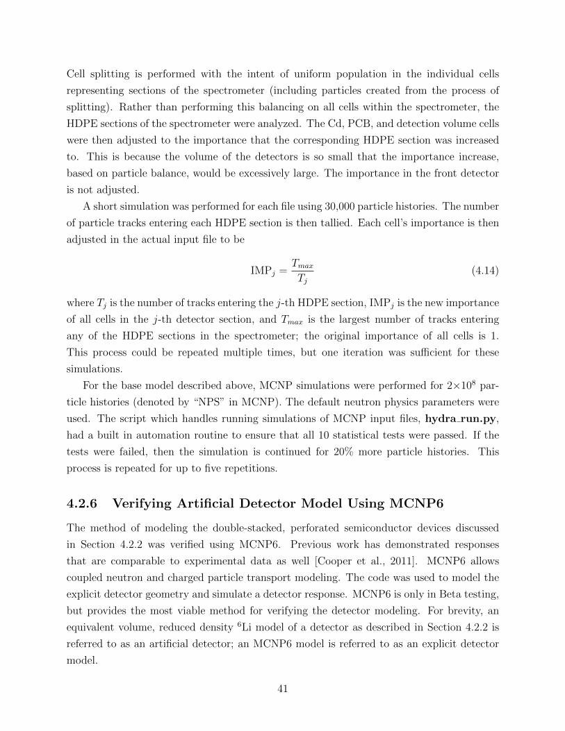
Cell splitting is performed with the intent of uniform population in the individual cells
representing sections of the spectrometer (including particles created from the process of
splitting). Rather than performing this balancing on all cells within the spectrometer, the
HDPE sections of the spectrometer were analyzed. The Cd, PCB, and detection volume cells
were then adjusted to the importance that the corresponding HDPE section was increased
to. This is because the volume of the detectors is so small that the importance increase,
based on particle balance, would be excessively large. The importance in the front detector
is not adjusted.
A short simulation was performed for each file using 30,000 particle histories. The number
of particle tracks entering each HDPE section is then tallied. Each cell’s importance is then
adjusted in the actual input file to be
IMPj =TmaxTj
(4.14)
where Tj is the number of tracks entering the j-th HDPE section, IMPj is the new importance
of all cells in the j-th detector section, and Tmax is the largest number of tracks entering
any of the HDPE sections in the spectrometer; the original importance of all cells is 1.
This process could be repeated multiple times, but one iteration was sufficient for these
simulations.
For the base model described above, MCNP simulations were performed for 2×10⁸ par-
ticle histories (denoted by “NPS” in MCNP). The default neutron physics parameters were
used. The script which handles running simulations of MCNP input files, hydra run.py,
had a built in automation routine to ensure that all 10 statistical tests were passed. If the
tests were failed, then the simulation is continued for 20% more particle histories. This
process is repeated for up to five repetitions.
4.2.6 Verifying Artificial Detector Model Using MCNP6
The method of modeling the double-stacked, perforated semiconductor devices discussed
in Section 4.2.2 was verified using MCNP6. Previous work has demonstrated responses
that are comparable to experimental data as well [Cooper et al., 2011]. MCNP6 allows
coupled neutron and charged particle transport modeling. The code was used to model the
explicit detector geometry and simulate a detector response. MCNP6 is only in Beta testing,
but provides the most viable method for verifying the detector modeling. For brevity, an
equivalent volume, reduced density 6Li model of a detector as described in Section 4.2.2 is
referred to as an artificial detector; an MCNP6 model is referred to as an explicit detector
model.
41
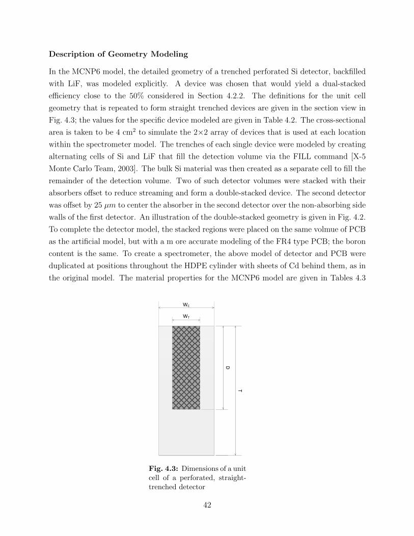
Description of Geometry Modeling
In the MCNP6 model, the detailed geometry of a trenched perforated Si detector, backfilled
with LiF, was modeled explicitly. A device was chosen that would yield a dual-stacked
efficiency close to the 50% considered in Section 4.2.2. The definitions for the unit cell
geometry that is repeated to form straight trenched devices are given in the section view in
Fig. 4.3; the values for the specific device modeled are given in Table 4.2. The cross-sectional
area is taken to be 4 cm2 to simulate the 2×2 array of devices that is used at each location
within the spectrometer model. The trenches of each single device were modeled by creating
alternating cells of Si and LiF that fill the detection volume via the FILL command [X-5
Monte Carlo Team, 2003]. The bulk Si material was then created as a separate cell to fill the
remainder of the detection volume. Two of such detector volumes were stacked with their
absorbers offset to reduce streaming and form a double-stacked device. The second detector
was offset by 25 µm to center the absorber in the second detector over the non-absorbing side
walls of the first detector. An illustration of the double-stacked geometry is given in Fig. 4.2.
To complete the detector model, the stacked regions were placed on the same volmue of PCB
as the artificial model, but with a m ore accurate modeling of the FR4 type PCB; the boron
content is the same. To create a spectrometer, the above model of detector and PCB were
duplicated at positions throughout the HDPE cylinder with sheets of Cd behind them, as in
the original model. The material properties for the MCNP6 model are given in Tables 4.3
WC
WT
D
T
Fig. 4.3: Dimensions of a unitcell of a perforated, straight-trenched detector
42
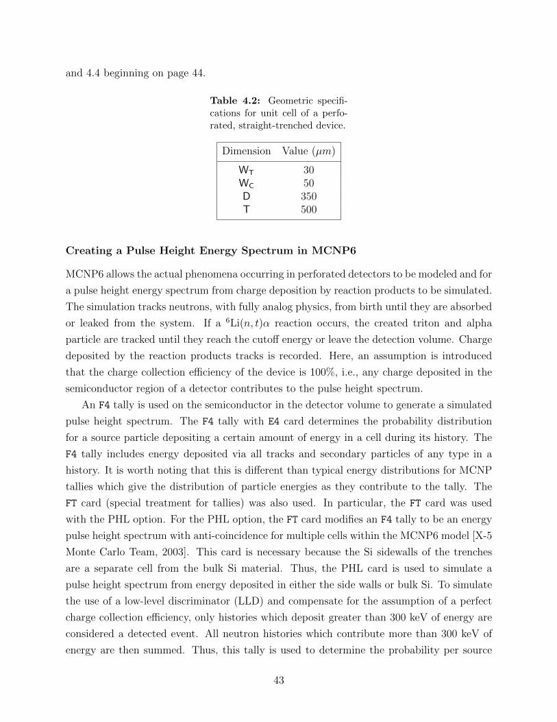
and 4.4 beginning on page 44.
Table 4.2: Geometric specifi-cations for unit cell of a perfo-rated, straight-trenched device.
Dimension Value (µm)
WT 30WC 50D 350T 500
Creating a Pulse Height Energy Spectrum in MCNP6
MCNP6 allows the actual phenomena occurring in perforated detectors to be modeled and for
a pulse height energy spectrum from charge deposition by reaction products to be simulated.
The simulation tracks neutrons, with fully analog physics, from birth until they are absorbed
or leaked from the system. If a 6Li(n, t)α reaction occurs, the created triton and alpha
particle are tracked until they reach the cutoff energy or leave the detection volume. Charge
deposited by the reaction products tracks is recorded. Here, an assumption is introduced
that the charge collection efficiency of the device is 100%, i.e., any charge deposited in the
semiconductor region of a detector contributes to the pulse height spectrum.
An F4 tally is used on the semiconductor in the detector volume to generate a simulated
pulse height spectrum. The F4 tally with E4 card determines the probability distribution
for a source particle depositing a certain amount of energy in a cell during its history. The
F4 tally includes energy deposited via all tracks and secondary particles of any type in a
history. It is worth noting that this is different than typical energy distributions for MCNP
tallies which give the distribution of particle energies as they contribute to the tally. The
FT card (special treatment for tallies) was also used. In particular, the FT card was used
with the PHL option. For the PHL option, the FT card modifies an F4 tally to be an energy
pulse height spectrum with anti-coincidence for multiple cells within the MCNP6 model [X-5
Monte Carlo Team, 2003]. This card is necessary because the Si sidewalls of the trenches
are a separate cell from the bulk Si material. Thus, the PHL card is used to simulate a
pulse height spectrum from energy deposited in either the side walls or bulk Si. To simulate
the use of a low-level discriminator (LLD) and compensate for the assumption of a perfect
charge collection efficiency, only histories which deposit greater than 300 keV of energy are
considered a detected event. All neutron histories which contribute more than 300 keV of
energy are then summed. Thus, this tally is used to determine the probability per source
43
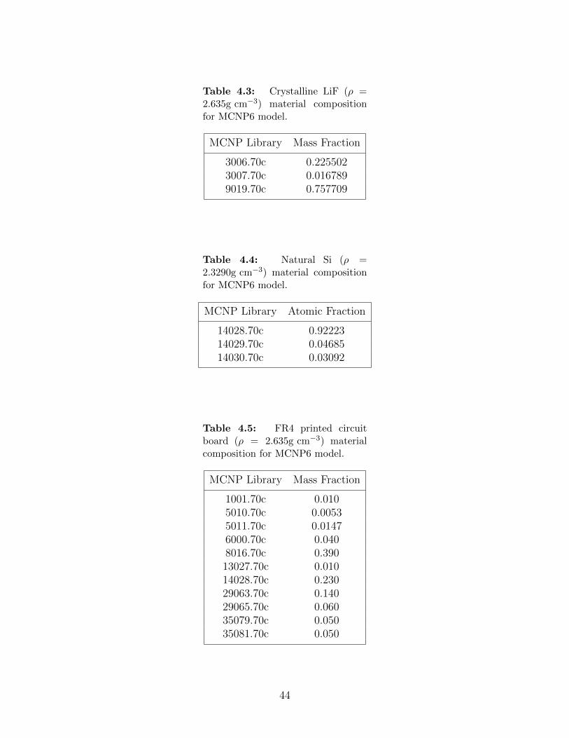
Table 4.3: Crystalline LiF (ρ =2.635g cm−3) material compositionfor MCNP6 model.
MCNP Library Mass Fraction
3006.70c 0.2255023007.70c 0.0167899019.70c 0.757709
Table 4.4: Natural Si (ρ =2.3290g cm−3) material compositionfor MCNP6 model.
MCNP Library Atomic Fraction
14028.70c 0.9222314029.70c 0.0468514030.70c 0.03092
Table 4.5: FR4 printed circuitboard (ρ = 2.635g cm−3) materialcomposition for MCNP6 model.
MCNP Library Mass Fraction
1001.70c 0.0105010.70c 0.00535011.70c 0.01476000.70c 0.0408016.70c 0.39013027.70c 0.01014028.70c 0.23029063.70c 0.14029065.70c 0.06035079.70c 0.05035081.70c 0.050
44
neutron of at least 300 keV of energy being deposited within the semiconductor region of
the detector.
Thermal Efficiency Verificiation
Efficiency simulation were performed in MCNP6 and MCNP5 to verify the artificial detector
model described in Section 4.2.2. First, the dual-stacked device placed on a PCB described in
Section 4.2.6 was modeled in MCNP6. The surface of the top detector was irradiated with a
thermal, normal-incident neutron beam of the same cross sectional area as the top detector.
The neutron beam was assumed to have a Maxwellian Energy distribution (see [X-5 Monte
Carlo Team, 2003]) with a mode of 0.0254 eV. The pulse height spectrum tally described in
Section 4.2.6 was used to determine the number of events that deposit greater than 300 keV
per source neutron. The number of particle histories simulated was 107.
The result of the thermal beam illuminating a double-stacked device produced 0.4728±0.0001
counts per source neutron. All source neutrons entered the device, thus the thermal efficiency
of this dual-stacked device was found to be 47.28±0.01%. This efficiency agrees with previous
simulations [Shultis and McGregor, 2009]. Using ε = 0.4728 in Eq. 4.10 yields an artificial6Li density of 0.07134 g cm−3. This density substituted into Eq. 4.13 yields C = 0.002857.
An MCNP5 input file was created using this C and ρ(6Li). The input file had the same
geometry and source specification as the MCNP6 model except for the detection region of
the explicit model was replaced with the artificial model. The tally method described in
Section 4.2.3 was used. 108 neutron histories were simulated. The only variance reduction
technique used in the artificial model is the default implicit capture method. The same 6Li
cross section library as the MCNP6 simulation was used, i.e., 3006.70c.
The MCNP5 simulation produced a thermal detector efficiency of 49.25± 0.01%. This is
in good agreement with the effiency of the MCNP6 simulation that was used to produce the
artificial model for the MCNP5 simulation. Accuracy is expected at thermal energies where
the large (n, t) cross section of 6Li dominates all interaction types.
Spectrometer Response Verification
A second scenario was simulated to verify the use of the artificial detector models. The
main phenomena of interest is streaming of high energy neutrons through the spectrometer.
Additionally, the accuracy of detector efficiency for the artificial model may be reduced when
neutrons entering the MSNDs are not uniform in direction, traversing the device at all angles.
Because only the relative responses are important in the FOM calculations, the detector
responses are normalized to the second detector. A spectrometer was modeled with five
45
detector positions and a 6.0 cm radius of the cylindrical HDPE sections. The front faces of
the detectors were 3.0 cm apart. The spectrometer model used the same detector and PCB
dimensions as the above results, with 0.1 cm of natural Cd behind each PCB. The beam
was of the same cross sectional area as the moderator. An MCNP6 and MCNP5 model
of the spectrometer were made. The only difference was the explicit and artificial detector
models for the MCNP6 and MCNP5 models, respectively. The number of histories for both
simulations was 109. The input file for the MCNP6 model is given on page 183.
Five different neutron sources were analyzed with both the MCNP5 and MCNP6 models:
AmBe, PuBe, a monoenergetic fusion source (14.1 MeV), and spontaneous fission sources of252Cf and 240Pu. The simulated detector spectrum from each source was normalized to the
second detector. The counts per source neutron and normalized detector responses, as well
as their associated errors, are given for each source simulation for the artificial and explicit
detector models are given in Table 4.6. A plot of the results from the 14.1 MeV, AmBe,
and PuBe sources is given in Fig. 4.4, and the results from spontaneous fission sources are
depicted in Fig. 4.5.
The unnormalized responses are inaccurate, particularly in the first detector, even though
the normalized responses appear to agree. The shape of the normalized curves, and how they
compare to each other, is all that is of interest; differences in the responses are compensated
for by increasing the number of neutrons. In all detector spectra, the artificial model slightly
overpredicts the explicit model, but is in good agreement. The main emphasis of the differ-
ence in the two models is that the spectrum shows the same shape, and that for different
sources the detector is higher. For 252Cf and 240Pu the simulated responses become very
close, and for one detector location, the artificial 252Cf response is higher than the 240Pu
response. This indicates that for this point, a 240Pu source may be incorrectly identified.
This simply suggests that care must be taken for sources that are close together, and that
these artificial templates although good enough for the process of optimization, may not be
able to be used as templates for identifying actual sources from experiment.
4.3 Geometric Optimization
4.3.1 Motivation
Simulations were performed to determine the optimal geometric configuration for the spec-
trometer. The optimal geometric configuration has the best ability to identify neutron
sources without additional complexity or weight from the moderator. The parameters that
were optimized for the spectrometer included the thickness of moderator between each de-
46
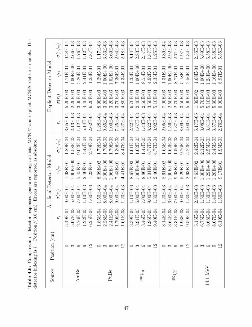
Tab
le4.6
:C
omp
aris
on
ofd
etec
tor
resp
onse
sge
ner
ated
usi
ng
arti
fici
alM
CN
P5
and
exp
lici
tM
CN
P6
det
ecto
rm
od
els.
Th
ed
etec
tor
ind
exin
gisi
=P
osi
tion/(
3.0
cm).
Err
ors
are
rep
orte
das
abso
lute
.
Sou
rce
Pos
itio
n(c
m)
Art
ifici
alD
etec
tor
Model
Explici
tD
etec
tor
Model
r iσ
(ri)
r i/r
2σ
(ri /r 2
)r i
σ(ri)
r i/r
2σ
(ri /r 2
)
Am
Be
05.
49E
-04
9.00
E-0
41.
08E
-01
1.89
E-0
43.
65E
-04
5.20
E-0
31.
71E
-01
9.28
E-0
43
5.07
E-0
35.
00E
-04
1.00
E+
001.
58E
-03
2.13
E-0
32.
20E
-03
1.00
E+
002.
66E
-03
62.
76E
-03
7.00
E-0
45.
45E
-01
9.02
E-0
41.
12E
-03
3.00
E-0
35.
26E
-01
1.76
E-0
39
1.22
E-0
31.
10E
-03
2.40
E-0
14.
47E
-04
5.14
E-0
44.
40E
-03
2.41
E-0
11.
12E
-03
126.
25E
-04
1.60
E-0
31.
23E
-01
2.70
E-0
42.
62E
-04
6.20
E-0
31.
23E
-01
7.87
E-0
4
PuB
e
01.
85E
-04
1.50
E-0
38.
09E
-02
1.72
E-0
41.
28E
-04
8.90
E-0
31.
29E
-01
1.17
E-0
33
2.28
E-0
38.
00E
-04
1.00
E+
001.
70E
-03
9.85
E-0
43.
20E
-03
1.00
E+
003.
53E
-03
62.
41E
-03
8.00
E-0
41.
06E
+00
1.79
E-0
31.
00E
-03
3.20
E-0
31.
02E
+00
3.60
E-0
39
1.70
E-0
39.
00E
-04
7.43
E-0
11.
30E
-03
7.25
E-0
43.
70E
-03
7.36
E-0
12.
94E
-03
121.
01E
-03
1.20
E-0
34.
41E
-01
8.47
E-0
44.
27E
-04
4.80
E-0
34.
34E
-01
2.18
E-0
3
240P
u
03.
39E
-04
1.10
E-0
38.
67E
-02
1.61
E-0
42.
22E
-04
6.70
E-0
31.
33E
-01
9.14
E-0
43
3.91
E-0
36.
00E
-04
1.00
E+
001.
62E
-03
1.67
E-0
32.
40E
-03
1.00
E+
002.
83E
-03
63.
46E
-03
7.00
E-0
48.
86E
-01
1.47
E-0
31.
43E
-03
2.60
E-0
38.
55E
-01
2.57
E-0
39
1.96
E-0
39.
00E
-04
5.01
E-0
18.
77E
-04
8.22
E-0
43.
50E
-03
4.92
E-0
11.
87E
-03
129.
40E
-04
1.30
E-0
32.
40E
-01
4.77
E-0
43.
92E
-04
5.10
E-0
32.
35E
-01
1.25
E-0
3
252C
f
03.
14E
-04
1.20
E-0
38.
61E
-02
1.65
E-0
42.
05E
-04
7.00
E-0
31.
31E
-01
9.39
E-0
43
3.64
E-0
36.
00E
-04
1.00
E+
001.
62E
-03
1.56
E-0
32.
50E
-03
1.00
E+
002.
92E
-03
63.
31E
-03
7.00
E-0
49.
08E
-01
1.50
E-0
31.
37E
-03
2.70
E-0
38.
77E
-01
2.71
E-0
39
1.93
E-0
39.
00E
-04
5.29
E-0
19.
26E
-04
8.09
E-0
43.
50E
-03
5.18
E-0
11.
97E
-03
129.
59E
-04
1.30
E-0
32.
63E
-01
5.22
E-0
44.
00E
-04
5.00
E-0
32.
56E
-01
1.34
E-0
3
14.1
MeV
05.
15E
-05
2.80
E-0
37.
63E
-02
2.42
E-0
45.
17E
-05
1.39
E-0
21.
68E
-01
2.35
E-0
33
6.75
E-0
41.
50E
-03
1.00
E+
002.
12E
-03
3.08
E-0
45.
70E
-03
1.00
E+
005.
89E
-03
68.
68E
-04
1.30
E-0
31.
29E
+00
2.55
E-0
33.
81E
-04
5.10
E-0
31.
24E
+00
6.58
E-0
39
8.07
E-0
41.
40E
-03
1.20
E+
002.
45E
-03
3.57
E-0
45.
30E
-03
1.16
E+
006.
38E
-03
126.
19E
-04
1.50
E-0
39.
17E
-01
1.95
E-0
32.
76E
-04
6.00
E-0
38.
97E
-01
5.55
E-0
3
47
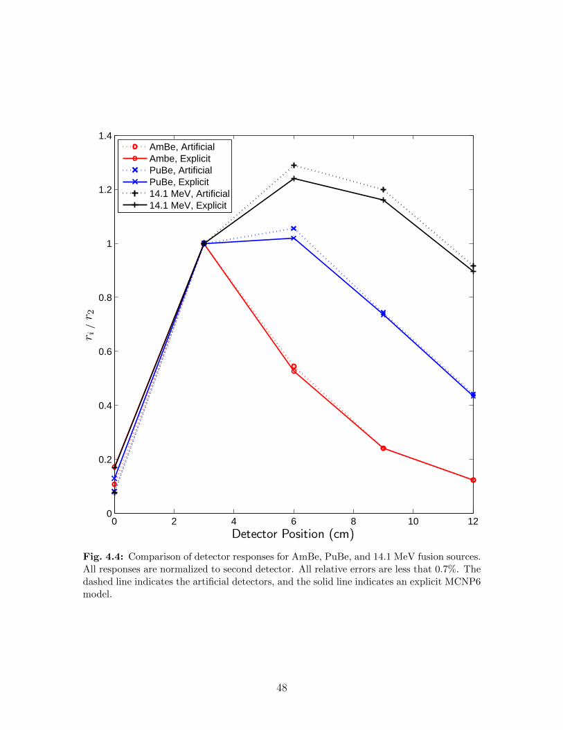
0 2 4 6 8 10 120
0.2
0.4
0.6
0.8
1
1.2
1.4
r i/r 2
Detector Position (cm)
AmBe, ArtificialAmbe, ExplicitPuBe, ArtificialPuBe, Explicit14.1 MeV, Artificial14.1 MeV, Explicit
Fig. 4.4: Comparison of detector responses for AmBe, PuBe, and 14.1 MeV fusion sources.All responses are normalized to second detector. All relative errors are less that 0.7%. Thedashed line indicates the artificial detectors, and the solid line indicates an explicit MCNP6model.
48
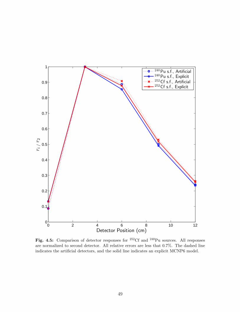
0 2 4 6 8 10 120
0.1
0.2
0.3
0.4
0.5
0.6
0.7
0.8
0.9
1
r i/r 2
Detector Position (cm)
240Pu s.f., Artificial240Pu s.f., Explicit252Cf s.f., Artificial252Cf s.f., Explicit
Fig. 4.5: Comparison of detector responses for 252Cf and 240Pu sources. All responsesare normalized to second detector. All relative errors are less that 0.7%. The dashed lineindicates the artificial detectors, and the solid line indicates an explicit MCNP6 model.
49
tector, the cross sectional area of the moderator, and the number of detectors in the spec-
trometer. The weight of the device was also considered, but a specific weight criteria was not
specified other than usability as a hand-held device. The optimization was multidimensional
and thus performed in several iterative steps. As there were minimal design criteria for the
device, several constraints for the optimization were set based on initial simulation results. A
general brute-force search was employed for optimization, as the tolerance on optimizations
is sufficiently imprecise that more precise methods are not necessary.
4.3.2 Development of Objective Function
An objective function was developed to compare geometries based on their ability to identify
sources via FOM values. An objective function provides a quantifiable measure of the
quality of the results for a particular set of optimization parameters. Either the minimum
or maximum of the objective function, depending on the definition of the function, provides
the optimal set of parameters.
The goal of a spectrometer is to identify all sources accurately and with statistical con-
fidence. For a particular experimentally measured spectrum, a FOM value is generated for
each reference spectrum in the library. For correct identification of the neutron source, the
lowest calculated FOM value should correspond to the reference spectrum associated with
that source; the difference between the lowest value and the next closest must also be statis-
tically significant for the source to have been identified with confidence. Thus, a deviation is
formed for a particular source as the difference between the lowest and second lowest FOM
values, relative to the larger uncertainty of the two values, i.e.,
∆ =FOMmin+ − FOMmin
σ(FOMmin+), (4.15)
where FOMmin is the lowest FOM value, FOMmin+ is the second lowest FOM value, and
σ(FOMmin+) is the standard deviation of FOMmin+. The largest uncertainty of the two
FOM values is σ(FOMmin+) rather than σ(FOMmin) because σ(FOM) ∝√FOM . Us-
ing the larger of the two uncertainties is more conservative. By dividing by the standard
deviation, Eq. (4.15) removes any difference in FOM values caused by different numbers
of detectors (increasing the degrees of freedom which proportionally increases the expected
mean of FOM values). The spectrometer must be able to identify all neutron sources in a
set of reference spectra in this manner. The case in which the spectrometer identifies the
source with the lowest confidence is the minimum value of ∆ for the set of all possible sources
50
∆min = min ∆i : i = 1, 2, ..., Nsrc , (4.16)
where Nsrc is the number of sources reference spectra are available for. The set of values ∆iare stochastic, so ∆min is a random variable with some distribution. An expectation value
for ∆min can be determined by averaging ∆min for many measured spectra that provides
a measure of the ability of a particular geometry to discriminate between FOM values
for various sources. Thus, the objective function Θ for the spectrometer is taken as the
expectation value of ∆min, i.e.,
Θ =1
Ncorr
Ncorr∑n=1
∆(n)min. (4.17)
Here, ∆(n)min is the n-th ∆min of Ncorr trials in which all sources were correctly identified.
Each trial contains a measured spectra for each of the Nsrc sources. It is noted that Ntrials is
the total number of trials simulated; however, Ncorr in Eq. (4.17) only includes trials which
identify all sources correctly. The sample standard deviation for Θ is computed as
σ(Θ) =1√
Ncorr − 1
√∆2
min −Θ2, (4.18)
where
∆2min =
1
Ncorr
Ncorr∑n=1
(∆(n)min)2, (4.19)
is the expected value of the square of ∆min.
For a correctly identified source, a relatively high value of Θ indicates a large difference
between the two lowest FOM values, relative to the statistical uncertainty in the values; this
is considered to indicate a higher quality spectrometer. The confidence of identification is
also dependent on the location of the lowest FOM value and its uncertainty. This is not
considered because in general if Θ is high, then the separation is high, and the uncertainty
in the lowest detector is proportional to the square root of that FOM.
The percentage of the Ntrials that correctly identify a source is also tabulated as a statistic
and considered a measure of quality. Here, frequentist statistics is assumed. Explicitly,
P (correct identification of all Sources in a trial) = psucc, where
psucc =# of trials where all sources were correctly identified
Ntrials
. (4.20)
51
4.3.3 Simulated Responses
The calculation of FOM requires the comparison of an observed detector spectrum to a
reference spectrum. The reference spectra can be generated from the simulated detector
responses of an MCNP simulation. For the purpose of optimization, it is not feasible to
collect the many observed detector responses experimentally. As an alternative method,
measured detector spectra can be generated by using counting statistics to sample from the
reference spectra, as described in the remainder of this section. With artificially generated
data, Monte Carlo sampling can be used to generate FOM values.
To generate an observed detector spectra, a response is sampled from an appropriate
PDF for each detector in the spectrometer. The type and parameters of the PDF depend
on the expected number of counts (i.e., the mean number of counts) present in the detector.
The number of counts observed in a detector is a random variable which follows a Poisson
distribution. A Poisson distribution for a random variable is fully defined by the mean of the
random variable. Thus, if the mean number of counts observed in a detector is known, the
observed number of counts is distributed as a Poisson distribution with that mean. Here,
electronic noise and other phenomena in a detector that would distort the distribution are
ignored.
The F4 MCNP tallies used to simulate detector responses discussed in Section 4.2.2
provide a normalized response function for each detector in the spectrometer. Each response
function estimates the expected value of counts observed in a particular detector, per source
neutron. The total number of source neutrons S0 multiplied by the response function can be
taken as the mean of the distribution that observed counts in such a detector would follow.
Therefore, for a particular neutron source strength, the simulated observed number of counts
in a detector would follow a Poisson distribution with a mean µ given by:
µi = S0ri. (4.21)
Here, ri is the MCNP response (tally) for the detector position of interest. For the MCNP
model used for optimization, the number of neutrons incident upon the spectrometer is the
same as S0 because the beam is uniform and of the same size as the cross sectional area of
the device. As a result, the nomenclature of neutron source strength is used throughout this
chapter to refer to the total number of neutrons incident upon the spectrometer.
In application, the spectrometer will count for some fixed period of time, so for a uniform
incident beam, the total incident neutrons would be given by
S0 = s0AT, (4.22)
52
where s0 is the neutron source strength per unit time per unit area (n cm−2 s−1 ), A is
the cross-sectional area of the spectrometer, and T is the total count time. It should be
remembered that this discussion is for a source beam of the same cross sectional area as the
device.
For the purpose of comparing spectrometers with different cross sectional areas, it is more
physically realistic to keep the source strength per unit area the same. Also, because T is a
variable that can be linearly scaled in application to achieve a particular value of S0, it has
no over all effect on optimizations. Thus, for a particular neutron field, the total number
of incident neutrons per unit area over a certain time s0 is kept constant when comparing
different spectrometer geometries. The relation between S0 and s0 for a uniform, normal
incident beam is s0 = S0/A. Although s0 remains constant, S0 is needed to determine
detector responses, and is thus typically used to characterize the neutron source strength in
this work.
A pseudo-random number generator is used to sample a random floating point number
between 0 and 1. This random number is transformed to sample values from the appro-
priate Poisson PDF. For large values of µ, sampling from a Poisson distribution becomes
computationally difficult and another method must be used. For a mean greater than 20,
a particular Poisson distribution can be well approximated by a Gaussian distribution with
the same mean as the Poisson distribution and a variance given by the square root of that
mean [Tsoulfanidis, 1995]. Combining these results with the distributions defined in Sec-
tion 2.1.5, the observed response in each detector is sampled from the PDF
f(N) =
1√2πσ
e−(µ−N)2/(2σ2) µ ≥ 20
µN
N !e−µ 0 ≤ µ < 20
. (4.23)
where σ =√µ is the standard deviation for the Gaussian PDF and N is rounded to be a
discrete number after sampling for the Gaussian PDF. The pseudo-random number generator
used was the Park and Miller Generator described in detail by Press et al. [1992]. The random
variable with a uniform distribution was transformed to the appropriate distributions for N
using methods and algorithms from Numerical Recipes by Press et al. [1992]. The Fortran90
code that performs the sampling is an executable generated from the simul resp.f90 source
code, found on page 166. The random number seed for the random number generator is
written to a file and passed between directories to ensure random numbers are not reused
across trials.
It is noted that when comparing different cross-sectional areas of the spectrometer, the
53
input to the simulated response codes for the source strength can be confusing. As mentioned
above, the source strength per unit area is kept constant, not the total number of neutrons
incident upon the spectrometer. However, the input for source strength in the codes is given
as the total number of incident neutrons. The source strength is scaled internally in the
code by cross-sectional area to keep the source strength per unit area constant. Explicitly,
the source strength that is input is scaled by the ratio of the cross-sectional area of the
spectrometer of interest to that of a 10-cm radius spectrometer.
4.4 Automation of Simulations and Data analysis
To automate the procedure of performing the large number of simulations and process-
ing data for optimization, a set of interconnected Python scripts (modules) was developed.
Python is an efficient scripting language with many integrated pre-existing numerical analy-
sis packages. In general, the Python modules created for the work described in this chapter
are a mix of procedural and object-oriented programs. For the numerical analysis portion of
the work, Fortran90 programs were written. These programs are executed using a Python
wrapper script. Appendix B summarizes the function of each Python module and Fortran90
program on page 135. The actual source code and scripts are included in Appendix B as well,
with the exception of straightforward modules. It is noted that the majority of the modules
were not sufficiently robust enough to perform all simulations of interest, so modifications
to the base code were made throughout.
The general procedure for performing simulations and data processing is as follows:
1. For each geometry and neutron source, create an MCNP input file.
2. Perform all MCNP simulations, ensuring that statistical tests are passed.
3. Organize output tallies from each file into individual tallies
4. For many trials:
(a) Simulate observed data from all sources
(b) Perform FOM calculations between all templates and simulated data
(c) Calculate Θ (and other parameters of interest) and add them to large data array
5. Average results from many trials
54
4.5 Corrections to the FOM for MCNP Simulations
Adjustments must be made to the FOM equations to correct for artificial biases in results
introduced by MCNP simulations in the σ(Sji ) term. The corrections are artificial and are
only necessary for optimization comparisons. The modified FOM statistic is given as
FOM j =
Ndet∑i=1
(Ri − Sji )2
σ2(Ri) + βradβNPS σ2(Sji ), (4.24)
where the factors βNPS and βrad are described below and all other factors are the same as
before. This equation was used for comparing all optimization simulations.
Cross Sectional Area of Moderator
Adjusting the cross-sectional area of the spectrometer requires adjustment to the uncertainty
σ(Sji ). The correction arises because tallies in MCNP are normalized to a response per source
neutron, rather than per source per unit area. To explain this correction, consider the tally
response of a particular detector in a spectrometer with some reference radius rref . In the
MCNP simulations, the source is a uniform disk of the same orientation and radius as the
spectrometer. In an analog sense, the tally gives the average response in the detector per
neutron from a total source strength equal to the number of particle histories, NPS. The tally
will have some sample standard deviation, σ(0). Now, consider a simulation with the same
value of NPS but a smaller radius r. In this case, because the value of NPS is the same, the
number of particle histories per source area has been increased, and thus particle histories
are more likely to contribute to the tally, producing a smaller relative error (the tally is
larger, but this is accounted for by how sampling is performed as discussed in Section 4.3.3).
The smaller uncertainty in the smaller radius case introduces a bias into the values of
σ(Sji ). For comparison purposes, it is not reasonable for the geometry with a smaller radius
to have a lower variance; in an experimentally collected template, a lower radius would not
have a lower variance as the source strength per unit area is the same. To correct the bias in
optimization simulations, a correction factor βrad is applied to the uncertainties, rather than
altering the value of NPS, to make all geometries have roughly equal relative errors. Scaling
the relative errors by a ratio of the areas, and applying error propagation, the result is
βrad =r2ref
r2. (4.25)
The value of rref is 10 cm for the optimization results in this chapter. The correction is
performed in the executable with source code fom.f90.
55
Different Number of Particle Histories
A similar bias occurs when different values of NPS are used. The value of NPS is increased
in some simulations to ensure that the 10 statistical tests in MCNP are passed. In general,
for all tallies σ ∝ 1/√NPS [X-5 Monte Carlo Team, 2003]. Thus, the correction factor is
βNPS =
√NPS
NPS(0), (4.26)
where NPS is the number of particle histories in the simulation which passes all statisti-
cal tests, and NPS(0) is the number of histories in the original simulation; all simulations
are performed for the same number of histories initially. For the optimization simula-
tions, NPS(0) = 2 × 10⁸. The correction for this factor takes place in the code module
FOM output.py.
4.6 Optimization Results
For all of the optimization results in this section, Eq. (4.17) was used to determine Θ, a mea-
sure of the quality of a spectrometer. In all cases, Ntrials = 1000 trials were performed. The
number of trials that all sources were correctly identified was calculated as psucc (Eq. (4.20)).
For each trial, observed detector spectra were generated for each neutron source using the
procedure described in Section 4.3.3. A uniform beam of incident neutrons was normally-
incident upon a spectrometer surrounded by a void, as described in Section 4.2.1. An
illustration of a spectrometer with labeled dimensions can be seen in Fig. 4.6. The integer
Ndet refers to the number of detector positions in a spectrometer.
The only two sources simulated for the optimization studies were the spontaneous fission
sources 240Pu and 252Cf. Only two sources were used for the optimization to limit the compu-
tational cost of simulations. Initial work determined that these two sources were consistently
the most difficult to distinguish because of their similar Watt energy spectra. If these sources
can be properly identified, all other sources should also be correctly identified. Additionally,
these two sources have neutrons covering the spectrum of most neutron sources, with the
exception of thermal neutrons. However, thermal neutrons are not a focus of optimization.
Because there is no moderator between the source and the front detector, thermal neutrons
are detected in the first detector, independent of the spectrometer geometry. It is of note
that the 240Pu source is exclusively fission neutrons from 240Pu, and does not include neu-
trons from induced fission from 239Pu that would be found in a mixture of 239Pu and 240Pu.
The energy spectrum of neutrons leaving a sphere of Pu with a mix of 239Pu and 240Pu is
56
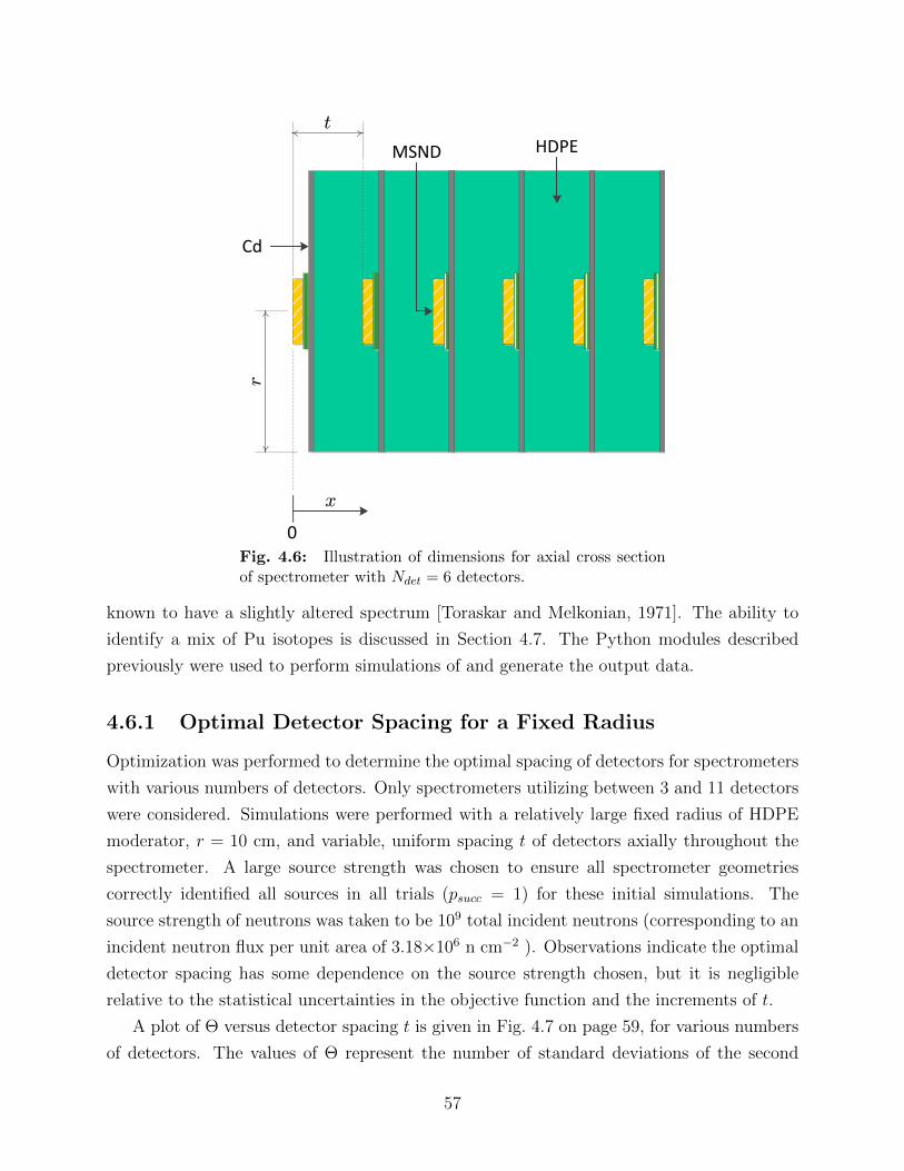
t
r
HDPEMSND
Cd
x
0Fig. 4.6: Illustration of dimensions for axial cross sectionof spectrometer with Ndet = 6 detectors.
known to have a slightly altered spectrum [Toraskar and Melkonian, 1971]. The ability to
identify a mix of Pu isotopes is discussed in Section 4.7. The Python modules described
previously were used to perform simulations of and generate the output data.
4.6.1 Optimal Detector Spacing for a Fixed Radius
Optimization was performed to determine the optimal spacing of detectors for spectrometers
with various numbers of detectors. Only spectrometers utilizing between 3 and 11 detectors
were considered. Simulations were performed with a relatively large fixed radius of HDPE
moderator, r = 10 cm, and variable, uniform spacing t of detectors axially throughout the
spectrometer. A large source strength was chosen to ensure all spectrometer geometries
correctly identified all sources in all trials (psucc = 1) for these initial simulations. The
source strength of neutrons was taken to be 109 total incident neutrons (corresponding to an
incident neutron flux per unit area of 3.18×10⁶ n cm−2 ). Observations indicate the optimal
detector spacing has some dependence on the source strength chosen, but it is negligible
relative to the statistical uncertainties in the objective function and the increments of t.
A plot of Θ versus detector spacing t is given in Fig. 4.7 on page 59, for various numbers
of detectors. The values of Θ represent the number of standard deviations of the second
57
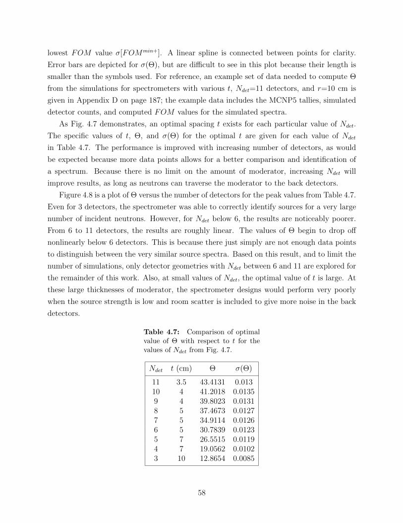
lowest FOM value σ[FOMmin+]. A linear spline is connected between points for clarity.
Error bars are depicted for σ(Θ), but are difficult to see in this plot because their length is
smaller than the symbols used. For reference, an example set of data needed to compute Θ
from the simulations for spectrometers with various t, Ndet=11 detectors, and r=10 cm is
given in Appendix D on page 187; the example data includes the MCNP5 tallies, simulated
detector counts, and computed FOM values for the simulated spectra.
As Fig. 4.7 demonstrates, an optimal spacing t exists for each particular value of Ndet.
The specific values of t, Θ, and σ(Θ) for the optimal t are given for each value of Ndet
in Table 4.7. The performance is improved with increasing number of detectors, as would
be expected because more data points allows for a better comparison and identification of
a spectrum. Because there is no limit on the amount of moderator, increasing Ndet will
improve results, as long as neutrons can traverse the moderator to the back detectors.
Figure 4.8 is a plot of Θ versus the number of detectors for the peak values from Table 4.7.
Even for 3 detectors, the spectrometer was able to correctly identify sources for a very large
number of incident neutrons. However, for Ndet below 6, the results are noticeably poorer.
From 6 to 11 detectors, the results are roughly linear. The values of Θ begin to drop off
nonlinearly below 6 detectors. This is because there just simply are not enough data points
to distinguish between the very similar source spectra. Based on this result, and to limit the
number of simulations, only detector geometries with Ndet between 6 and 11 are explored for
the remainder of this work. Also, at small values of Ndet, the optimal value of t is large. At
these large thicknesses of moderator, the spectrometer designs would perform very poorly
when the source strength is low and room scatter is included to give more noise in the back
detectors.
Table 4.7: Comparison of optimalvalue of Θ with respect to t for thevalues of Ndet from Fig. 4.7.
Ndet t (cm) Θ σ(Θ)
11 3.5 43.4131 0.01310 4 41.2018 0.01359 4 39.8023 0.01318 5 37.4673 0.01277 5 34.9114 0.01266 5 30.7839 0.01235 7 26.5515 0.01194 7 19.0562 0.01023 10 12.8654 0.0085
58
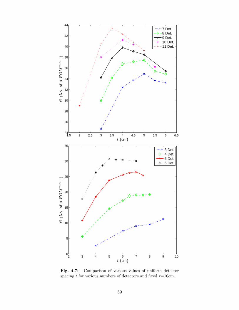
1.5 2 2.5 3 3.5 4 4.5 5 5.5 6 6.524
26
28
30
32
34
36
38
40
42
44
Θ(N
o.ofσ[F
OM
min
+])
t (cm)
7 Det.8 Det.9 Det.10 Det.11 Det.
2 3 4 5 6 7 8 9 100
5
10
15
20
25
30
35
Θ(N
o.ofσ[F
OM
min
+])
t (cm)
3 Det.4 Det.5 Det.6 Det.
Fig. 4.7: Comparison of various values of uniform detectorspacing t for various numbers of detectors and fixed r=10cm.
59
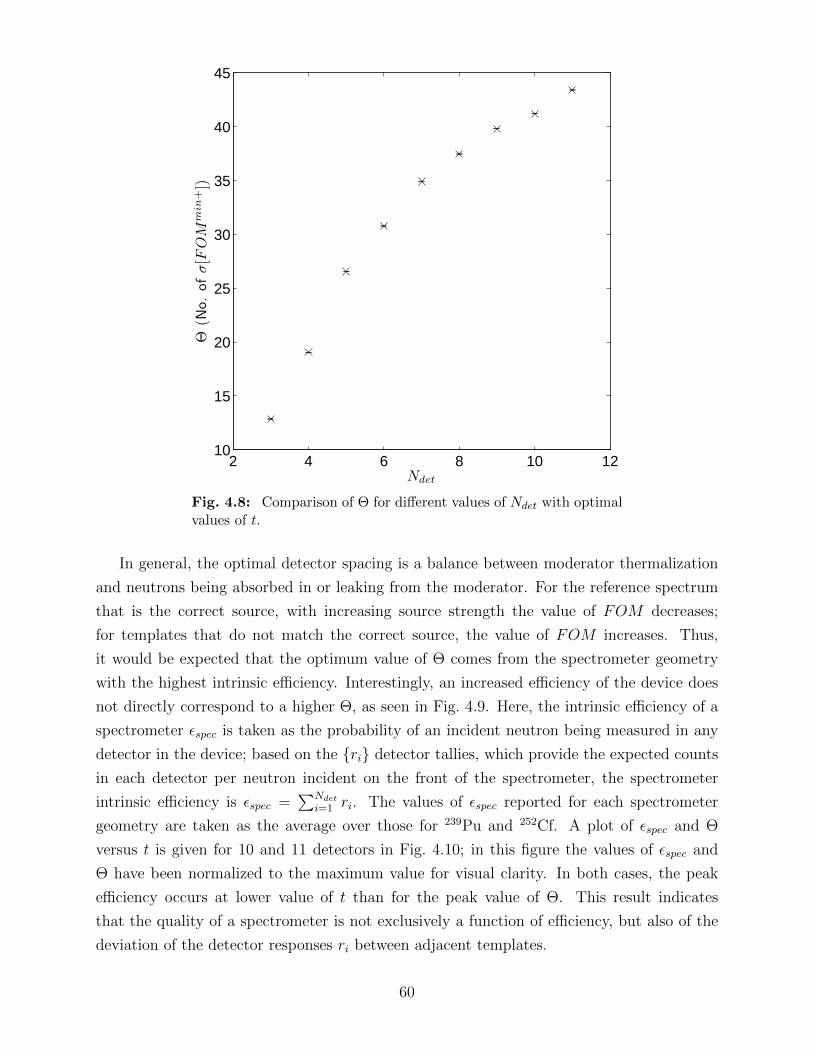
2 4 6 8 10 1210
15
20
25
30
35
40
45
Θ(N
o.ofσ[F
OM
min
+])
Ndet
Fig. 4.8: Comparison of Θ for different values of Ndet with optimalvalues of t.
In general, the optimal detector spacing is a balance between moderator thermalization
and neutrons being absorbed in or leaking from the moderator. For the reference spectrum
that is the correct source, with increasing source strength the value of FOM decreases;
for templates that do not match the correct source, the value of FOM increases. Thus,
it would be expected that the optimum value of Θ comes from the spectrometer geometry
with the highest intrinsic efficiency. Interestingly, an increased efficiency of the device does
not directly correspond to a higher Θ, as seen in Fig. 4.9. Here, the intrinsic efficiency of a
spectrometer εspec is taken as the probability of an incident neutron being measured in any
detector in the device; based on the ri detector tallies, which provide the expected counts
in each detector per neutron incident on the front of the spectrometer, the spectrometer
intrinsic efficiency is εspec =∑Ndet
i=1 ri. The values of εspec reported for each spectrometer
geometry are taken as the average over those for 239Pu and 252Cf. A plot of εspec and Θ
versus t is given for 10 and 11 detectors in Fig. 4.10; in this figure the values of εspec and
Θ have been normalized to the maximum value for visual clarity. In both cases, the peak
efficiency occurs at lower value of t than for the peak value of Θ. This result indicates
that the quality of a spectrometer is not exclusively a function of efficiency, but also of the
deviation of the detector responses ri between adjacent templates.
60
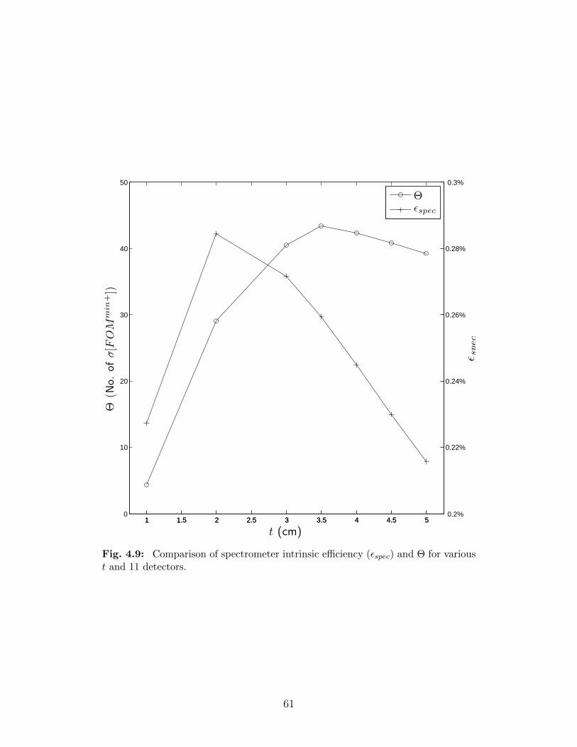
1 1.5 2 2.5 3 3.5 4 4.5 50
10
20
30
40
50
t (cm)
Θ(N
o.ofσ[F
OM
min
+])
1 1.5 2 2.5 3 3.5 4 4.5 5 0.2%
0.22%
0.24%
0.26%
0.28%
0.3%
ε spec
Θεspec
Fig. 4.9: Comparison of spectrometer intrinsic efficiency (εspec) and Θ for varioust and 11 detectors.
61
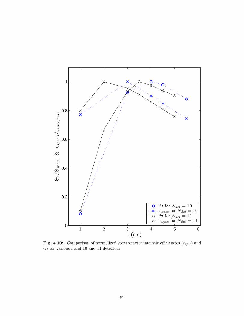
1 2 3 4 5 60
0.2
0.4
0.6
0.8
1
Θi/Θ
max
&ε s
pec,i/ε s
pec,m
ax
t (cm)
Θ for Ndet = 10εspec for Ndet = 10Θ for Ndet = 11εspec for Ndet = 11
Fig. 4.10: Comparison of normalized spectrometer intrinsic efficiencies (εspec) andΘs for various t and 10 and 11 detectors
62
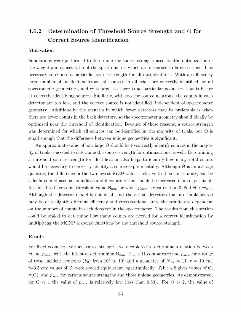
4.6.2 Determination of Threshold Source Strength and Θ for
Correct Source Identification
Motivation
Simulations were performed to determine the source strength used for the optimization of
the weight and aspect ratio of the spectrometer, which are discussed in later sections. It is
necessary to choose a particular source strength for all optimizations. With a sufficiently
large number of incident neutrons, all sources in all trials are correctly identified for all
spectrometer geometries, and Θ is large, so there is no particular geometry that is better
at correctly identifying sources. Similarly, with too few source neutrons, the counts in each
detector are too few, and the correct source is not identified, independent of spectrometer
geometry. Additionally, the scenario in which fewer detectors may be preferable is when
there are lower counts in the back detectors, so the spectrometer geometry should ideally be
optimized near the threshold of identification. Because of these reasons, a source strength
was determined for which all sources can be identified in the majority of trials, but Θ is
small enough that the difference between unique geometries is significant.
An approximate value of how large Θ should be to correctly identify sources in the major-
ity of trials is needed to determine the source strength for optimizations as well. Determining
a threshold source strength for identification also helps to identify how many total counts
would be necessary to correctly identify a source experimentally. Although Θ is an average
quantity, the difference in the two lowest FOM values, relative to their uncertainty, can be
calculated and used as an indicator of if counting time should be increased in an experiment.
It is ideal to have some threshold value Θmin for which psucc is greater than 0.95 if Θ > Θmin.
Although the detector model is not ideal, and the actual detectors that are implemented
may be of a slightly different efficiency and cross-sectional area, the results are dependent
on the number of counts in each detector in the spectrometer. The results from this section
could be scaled to determine how many counts are needed for a correct identification by
multiplying the MCNP response functions by the threshold source strength.
Results
For fixed geometry, various source strengths were explored to determine a relation between
Θ and psucc, with the intent of determining Θmin. Fig. 4.11 compares Θ and psucc for a range
of total incident neutrons (S0) from 105 to 107 and a geometry of Ndet = 11, r = 10 cm,
t=3.5 cm; values of S0 were spaced equidistant logarithmically. Table 4.8 gives values of Θ,
σ(Θ), and psucc for various source strengths and three unique geometries. As demonstrated,
for Θ < 1 the value of psucc is relatively low (less than 0.80). For Θ > 2, the value of
63
psucc is much higher (greater than 0.99 in all cases). Therefore, it is proposed that values of
Θ greater than 2 have at least a 95% statistical confidence of correct source identification,
and values of Θ < 1 have no statistical significance of correct identification. It is noted
that no general relation between confidence of identification and Θ is made here, other than
these two proposed limits. The true distribution of Θ is unknown, and σ(FOM) is a very
approximate standard deviation. The values of Θ are formed with data randomly sampled
from the precise means of distributions. In reality, because of neutrons scattering from the
room, detector noise, and general differences between simulation and reality, the observed
data points will be different than the means of the distributions. This will result in the
values of FOM that correspond to the correct source being much larger than the ones found
here. This may require the cutoff for theta to be higher, and that the relation between psucc
and Θ may demonstrate a different trend. Caution is advised in application of these results.
However, for optimization purposes, a value of Θmin = 2.0 is more than sufficient.
Several sample statistics of ∆(n)min (described by Eq. (4.16)) were computed for the Ncorr
trials where sources were correctly identified; the sample statistics are compared for various
source strengths. The sample standard deviation of ∆(n)min for n = 1, 2, . . . , Ncorr, notated
σ(∆(n)min), is given in Table 4.9. The average of the ∆(n)
min is Θ. The minimum and maximum
values of ∆(n)min from the Ncorr trials1 are also compared. For Θ > 2, the values of ∆
(n)min are
fairly centralized around the mean, justifying the value of Θmin = 2 being used as a similar
threshold of identification for ∆(n)min with individual measured spectra in application.
With a value of Θmin set, various values of S0 were explored for a variety of geometries
to determine a source strength for the remainder of optimization simulations. Geometries
that cover the spectrum of possible designs from 6 to 11 detectors were chosen for this set
of simulations. The value of t for each value of Ndet was based on the results for optimal
spacing from Table 4.7. Fig. 4.12 gives a plot of Θ versus the number of detectors (with
respective optimal thicknesses), for various values of S0. For 106 source neutrons, Θ was
near 1 or slightly below for all 3 geometries, whereas for 107, Θ was well above 3 in all cases.
Thus, 107 is taken to be the value of S0 for correct identification in the majority of trials, for
all geometries, and used for the remainder of optimizations; this corresponds to a neutron
source strength of 3.18×10⁴ n cm−2 . The source strength is only determined to best order of
magnitude because simulated detector efficiencies are not accurate necessarily with the real
design, and the strength is primarily for optimization purposes. Also, the source strength
chosen produces a Θ well above Θmin = 2 for all geometries, which is favorable because the
amount of moderator is later decreased in Section 4.6.3.
1It is noted for clarity that ∆(n)min is the minimum value of the ∆i : i = 1, 2, . . . , Ntemp for the n-th trial
(in this case there are only two templates), and min∆(n)min is the minimum of that value from all trials.
64
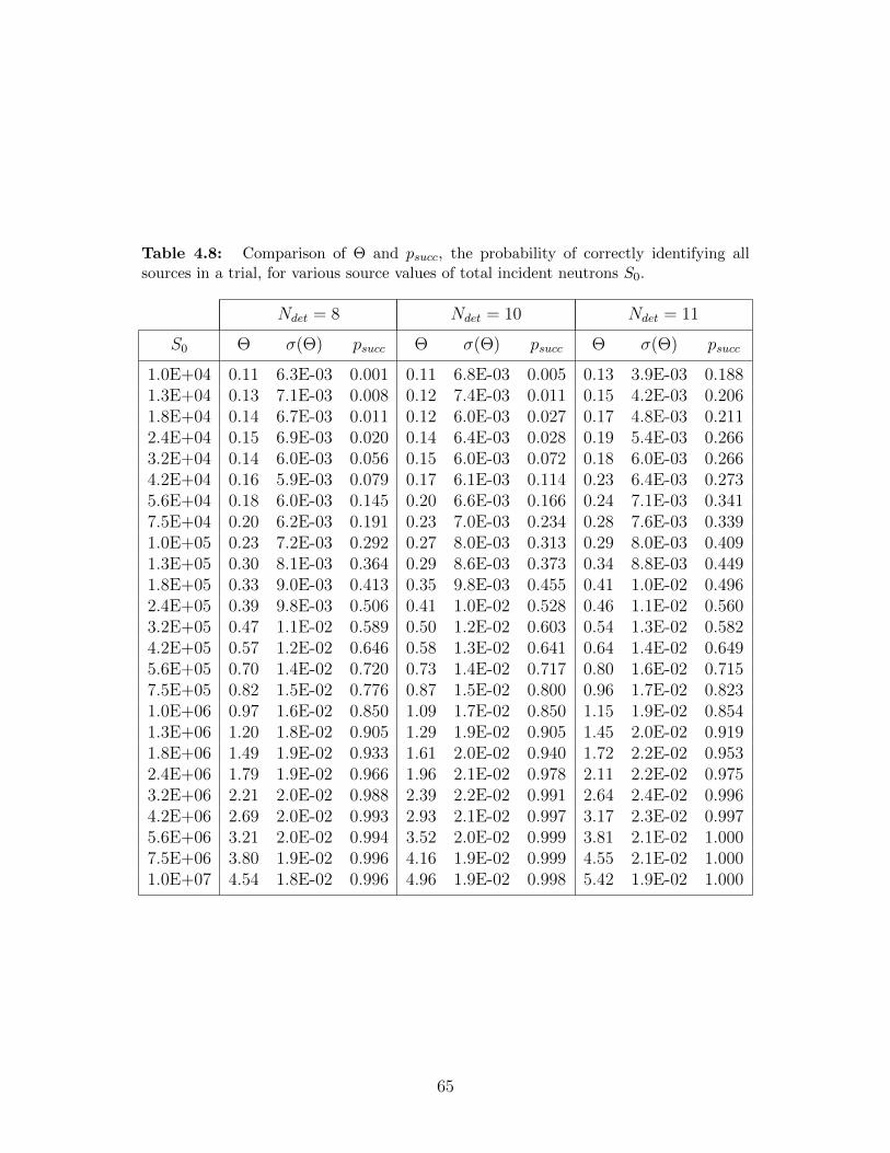
Table 4.8: Comparison of Θ and psucc, the probability of correctly identifying allsources in a trial, for various source values of total incident neutrons S0.
Ndet = 8 Ndet = 10 Ndet = 11
S0 Θ σ(Θ) psucc Θ σ(Θ) psucc Θ σ(Θ) psucc
1.0E+04 0.11 6.3E-03 0.001 0.11 6.8E-03 0.005 0.13 3.9E-03 0.1881.3E+04 0.13 7.1E-03 0.008 0.12 7.4E-03 0.011 0.15 4.2E-03 0.2061.8E+04 0.14 6.7E-03 0.011 0.12 6.0E-03 0.027 0.17 4.8E-03 0.2112.4E+04 0.15 6.9E-03 0.020 0.14 6.4E-03 0.028 0.19 5.4E-03 0.2663.2E+04 0.14 6.0E-03 0.056 0.15 6.0E-03 0.072 0.18 6.0E-03 0.2664.2E+04 0.16 5.9E-03 0.079 0.17 6.1E-03 0.114 0.23 6.4E-03 0.2735.6E+04 0.18 6.0E-03 0.145 0.20 6.6E-03 0.166 0.24 7.1E-03 0.3417.5E+04 0.20 6.2E-03 0.191 0.23 7.0E-03 0.234 0.28 7.6E-03 0.3391.0E+05 0.23 7.2E-03 0.292 0.27 8.0E-03 0.313 0.29 8.0E-03 0.4091.3E+05 0.30 8.1E-03 0.364 0.29 8.6E-03 0.373 0.34 8.8E-03 0.4491.8E+05 0.33 9.0E-03 0.413 0.35 9.8E-03 0.455 0.41 1.0E-02 0.4962.4E+05 0.39 9.8E-03 0.506 0.41 1.0E-02 0.528 0.46 1.1E-02 0.5603.2E+05 0.47 1.1E-02 0.589 0.50 1.2E-02 0.603 0.54 1.3E-02 0.5824.2E+05 0.57 1.2E-02 0.646 0.58 1.3E-02 0.641 0.64 1.4E-02 0.6495.6E+05 0.70 1.4E-02 0.720 0.73 1.4E-02 0.717 0.80 1.6E-02 0.7157.5E+05 0.82 1.5E-02 0.776 0.87 1.5E-02 0.800 0.96 1.7E-02 0.8231.0E+06 0.97 1.6E-02 0.850 1.09 1.7E-02 0.850 1.15 1.9E-02 0.8541.3E+06 1.20 1.8E-02 0.905 1.29 1.9E-02 0.905 1.45 2.0E-02 0.9191.8E+06 1.49 1.9E-02 0.933 1.61 2.0E-02 0.940 1.72 2.2E-02 0.9532.4E+06 1.79 1.9E-02 0.966 1.96 2.1E-02 0.978 2.11 2.2E-02 0.9753.2E+06 2.21 2.0E-02 0.988 2.39 2.2E-02 0.991 2.64 2.4E-02 0.9964.2E+06 2.69 2.0E-02 0.993 2.93 2.1E-02 0.997 3.17 2.3E-02 0.9975.6E+06 3.21 2.0E-02 0.994 3.52 2.0E-02 0.999 3.81 2.1E-02 1.0007.5E+06 3.80 1.9E-02 0.996 4.16 1.9E-02 0.999 4.55 2.1E-02 1.0001.0E+07 4.54 1.8E-02 0.996 4.96 1.9E-02 0.998 5.42 1.9E-02 1.000
65
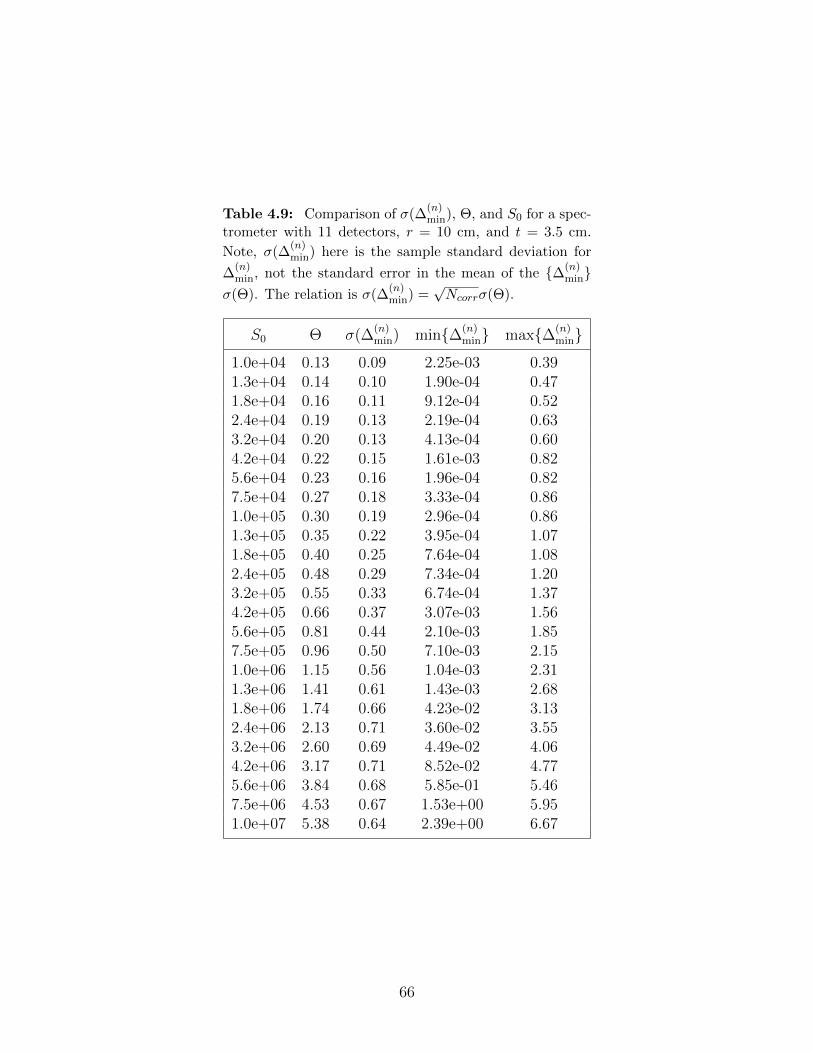
Table 4.9: Comparison of σ(∆(n)min), Θ, and S0 for a spec-
trometer with 11 detectors, r = 10 cm, and t = 3.5 cm.
Note, σ(∆(n)min) here is the sample standard deviation for
∆(n)min, not the standard error in the mean of the ∆(n)
minσ(Θ). The relation is σ(∆
(n)min) =
√Ncorrσ(Θ).
S0 Θ σ(∆(n)min) min∆(n)
min max∆(n)min
1.0e+04 0.13 0.09 2.25e-03 0.391.3e+04 0.14 0.10 1.90e-04 0.471.8e+04 0.16 0.11 9.12e-04 0.522.4e+04 0.19 0.13 2.19e-04 0.633.2e+04 0.20 0.13 4.13e-04 0.604.2e+04 0.22 0.15 1.61e-03 0.825.6e+04 0.23 0.16 1.96e-04 0.827.5e+04 0.27 0.18 3.33e-04 0.861.0e+05 0.30 0.19 2.96e-04 0.861.3e+05 0.35 0.22 3.95e-04 1.071.8e+05 0.40 0.25 7.64e-04 1.082.4e+05 0.48 0.29 7.34e-04 1.203.2e+05 0.55 0.33 6.74e-04 1.374.2e+05 0.66 0.37 3.07e-03 1.565.6e+05 0.81 0.44 2.10e-03 1.857.5e+05 0.96 0.50 7.10e-03 2.151.0e+06 1.15 0.56 1.04e-03 2.311.3e+06 1.41 0.61 1.43e-03 2.681.8e+06 1.74 0.66 4.23e-02 3.132.4e+06 2.13 0.71 3.60e-02 3.553.2e+06 2.60 0.69 4.49e-02 4.064.2e+06 3.17 0.71 8.52e-02 4.775.6e+06 3.84 0.68 5.85e-01 5.467.5e+06 4.53 0.67 1.53e+00 5.951.0e+07 5.38 0.64 2.39e+00 6.67
66
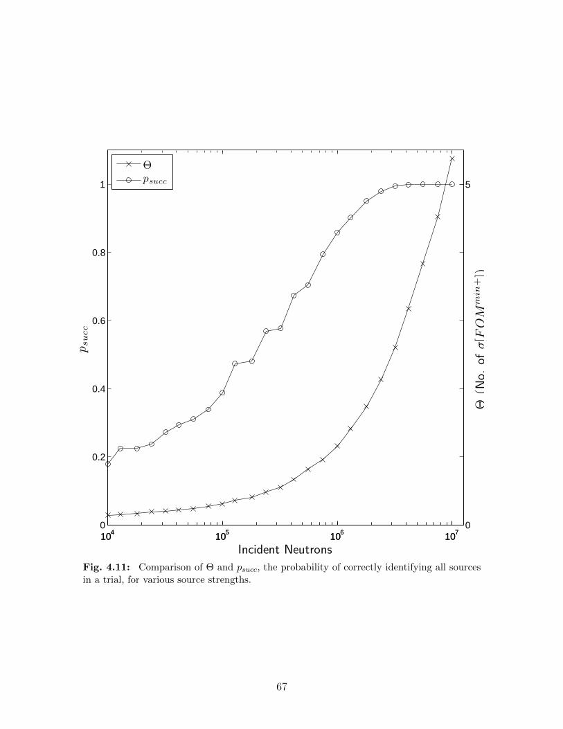
104 105 106 1070
0.2
0.4
0.6
0.8
1
psucc
Incident Neutrons104 105 106 107
0
5
Θ(N
o.ofσ[F
OM
min
+])
Θpsucc
Fig. 4.11: Comparison of Θ and psucc, the probability of correctly identifying all sourcesin a trial, for various source strengths.
67
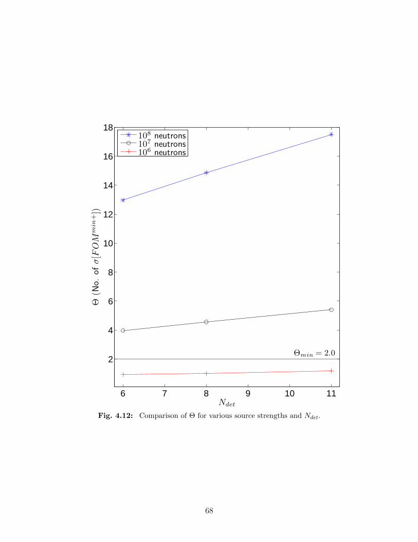
6 7 8 9 10 11
2
4
6
8
10
12
14
16
18
Θ(N
o.ofσ[F
OM
min
+])
Ndet
Θmin = 2.0
108 neutrons107 neutrons106 neutrons
Fig. 4.12: Comparison of Θ for various source strengths and Ndet.
68
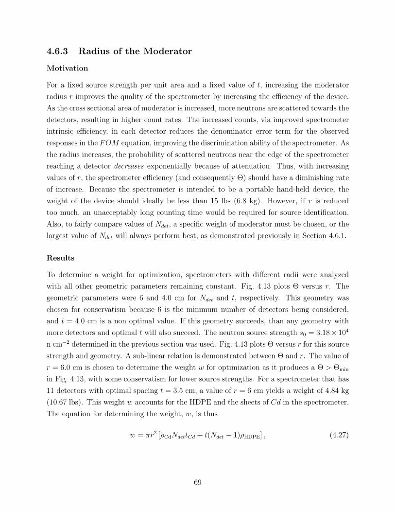
4.6.3 Radius of the Moderator
Motivation
For a fixed source strength per unit area and a fixed value of t, increasing the moderator
radius r improves the quality of the spectrometer by increasing the efficiency of the device.
As the cross sectional area of moderator is increased, more neutrons are scattered towards the
detectors, resulting in higher count rates. The increased counts, via improved spectrometer
intrinsic efficiency, in each detector reduces the denominator error term for the observed
responses in the FOM equation, improving the discrimination ability of the spectrometer. As
the radius increases, the probability of scattered neutrons near the edge of the spectrometer
reaching a detector decreases exponentially because of attenuation. Thus, with increasing
values of r, the spectrometer efficiency (and consequently Θ) should have a diminishing rate
of increase. Because the spectrometer is intended to be a portable hand-held device, the
weight of the device should ideally be less than 15 lbs (6.8 kg). However, if r is reduced
too much, an unacceptably long counting time would be required for source identification.
Also, to fairly compare values of Ndet, a specific weight of moderator must be chosen, or the
largest value of Ndet will always perform best, as demonstrated previously in Section 4.6.1.
Results
To determine a weight for optimization, spectrometers with different radii were analyzed
with all other geometric parameters remaining constant. Fig. 4.13 plots Θ versus r. The
geometric parameters were 6 and 4.0 cm for Ndet and t, respectively. This geometry was
chosen for conservatism because 6 is the minimum number of detectors being considered,
and t = 4.0 cm is a non optimal value. If this geometry succeeds, than any geometry with
more detectors and optimal t will also succeed. The neutron source strength s0 = 3.18× 10⁴
n cm−2 determined in the previous section was used. Fig. 4.13 plots Θ versus r for this source
strength and geometry. A sub-linear relation is demonstrated between Θ and r. The value of
r = 6.0 cm is chosen to determine the weight w for optimization as it produces a Θ > Θmin
in Fig. 4.13, with some conservatism for lower source strengths. For a spectrometer that has
11 detectors with optimal spacing t = 3.5 cm, a value of r = 6 cm yields a weight of 4.84 kg
(10.67 lbs). This weight w accounts for the HDPE and the sheets of Cd in the spectrometer.
The equation for determining the weight, w, is thus
w = πr2 [ρCdNdettCd + t(Ndet − 1)ρHDPE] , (4.27)
69
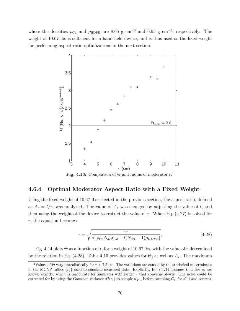
where the densities ρCd and ρHDPE are 8.65 g cm−3 and 0.95 g cm−3, respectively. The
weight of 10.67 lbs is sufficient for a hand held device, and is thus used as the fixed weight
for performing aspect ratio optimizations in the next section.
3 4 5 6 7 8 9 10 111
1.5
2
2.5
3
3.5
4Θ
(No.ofσ[F
OM
min
+])
r (cm)
Θmin = 2.0
Fig. 4.13: Comparison of Θ and radius of moderator r.1
4.6.4 Optimal Moderator Aspect Ratio with a Fixed Weight
Using the fixed weight of 10.67 lbs selected in the previous section, the aspect ratio, defined
as Ar = t/r, was analyzed. The value of Ar was changed by adjusting the value of t, and
then using the weight of the device to restrict the value of r. When Eq. (4.27) is solved for
r, the equation becomes
r =
√w
π [ρCdNdettCd + t(Ndet − 1)ρHDPE], (4.28)
Fig. 4.14 plots Θ as a function of t, for a weight of 10.67 lbs, with the value of r determined
by the relation in Eq. (4.28). Table 4.10 provides values for Θ, as well as Ar. The maximum
1Values of Θ vary unrealistically for r > 7.5 cm. The variations are caused by the statistical uncertaintiesin the MCNP tallies rji used to simulate measured data. Explicitly, Eq. (4.21) assumes that the µi areknown exactly, which is inaccurate for simulates with larger r that converge slowly. The noise could becorrected for by using the Gaussian variance σ2(ri) to sample a µi, before sampling Ci, for all i and sources.
70
2 2.5 3 3.5 4 4.5
2.4
2.6
2.8
3
3.2
3.4
3.6
3.8
Θ(N
o.ofσ[F
OM
min
+])
t (cm)
Ndet = 9Ndet = 10Ndet = 11
2.5 3 3.5 4 4.5 5 5.52.4
2.6
2.8
3
3.2
3.4
3.6
Θ(N
o.ofσ[F
OM
min
+])
t (cm)
Ndet = 6Ndet = 8
Fig. 4.14: Comparison of Θ for different geometries with afixed value of w of 4.84 kg.
71
values are slightly different in this case as compared to the fixed radius results. It is of
note that for a fixed weight, the 10 detector case performs very similarly to the 11 detectors
case (the optima agree within one standard deviation). So, for the same weight (the main
constraint on optimization), the number of detectors becomes relatively negligible at 10
detectors. With some conservatism, 11 detectors is a sufficient number of detector positions.
To determine if the aspect ratio (a dimensionless parameter) is the key factor in the quality
of the spectrometer, this process was repeated for different weights for the 9, 10, and 11
detector cases and found to produce optima at the same values of Ar , at least for the coarse
spacing used here.
Table 4.10: Comparison of aspect ratios and Θfor a variety of Ndet and a fixed weight of w at4.84 kg.
Ndet r t Ar Θ σ(Θ)
6 7.61 4.5 0.591 3.17 0.0217 7.69 3.5 0.455 3.35 0.0228 7.14 3.5 0.490 3.50 0.0229 6.69 3.5 0.523 3.48 0.02110 6.70 3.0 0.448 3.56 0.02211 6.80 2.5 0.368 3.59 0.026
4.7 Detecting WGPu versus 240Pu
The difference in energy spectra between 240Pu and Weapons Grade Plutonium (WGPu) is
due to the difference between energy of neutrons released from induced fission of 239Pu and
spontaneous fission of 240Pu [Toraskar and Melkonian, 1971]. The optimization simulations
were performed using the spontaneous fission energy spectrum of 240Pu. To determine the
ability of the spectrometer to identify a source of WGPu, simulations were performed and
compared against that of the pure 240Pu case.
The energy spectrum of WGPu is primarily a mix of neutrons from spontaneous fission
of 240Pu and induced fission of 239Pu, some of which will be moderated to lower energies.
The fractions of neutrons from induced and spontaneous fission will depend on the size and
mixture of the WGPu. The larger the device is, the more readily induced fissions will occur,
thus shifting the spectrum to consist more of energy of induced fission neutrons. The exact
mixture and density of WGPu can vary, and in general is not known. For the simulations
in this section, WGPu is taken to be a 4.0 kg sphere of a homogeneous mixture of 93%
72
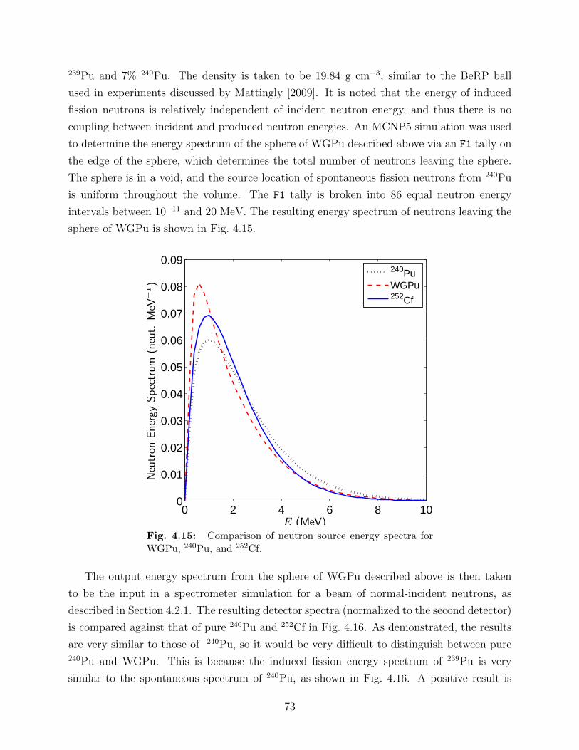
239Pu and 7% 240Pu. The density is taken to be 19.84 g cm−3, similar to the BeRP ball
used in experiments discussed by Mattingly [2009]. It is noted that the energy of induced
fission neutrons is relatively independent of incident neutron energy, and thus there is no
coupling between incident and produced neutron energies. An MCNP5 simulation was used
to determine the energy spectrum of the sphere of WGPu described above via an F1 tally on
the edge of the sphere, which determines the total number of neutrons leaving the sphere.
The sphere is in a void, and the source location of spontaneous fission neutrons from 240Pu
is uniform throughout the volume. The F1 tally is broken into 86 equal neutron energy
intervals between 10−11 and 20 MeV. The resulting energy spectrum of neutrons leaving the
sphere of WGPu is shown in Fig. 4.15.
0 2 4 6 8 100
0.01
0.02
0.03
0.04
0.05
0.06
0.07
0.08
0.09
E (MeV)
NeutronEnergySpectrum
(neut.
MeV
−1)
240PuWGPu252Cf
Fig. 4.15: Comparison of neutron source energy spectra forWGPu, 240Pu, and 252Cf.
The output energy spectrum from the sphere of WGPu described above is then taken
to be the input in a spectrometer simulation for a beam of normal-incident neutrons, as
described in Section 4.2.1. The resulting detector spectra (normalized to the second detector)
is compared against that of pure 240Pu and 252Cf in Fig. 4.16. As demonstrated, the results
are very similar to those of 240Pu, so it would be very difficult to distinguish between pure240Pu and WGPu. This is because the induced fission energy spectrum of 239Pu is very
similar to the spontaneous spectrum of 240Pu, as shown in Fig. 4.16. A positive result is
73
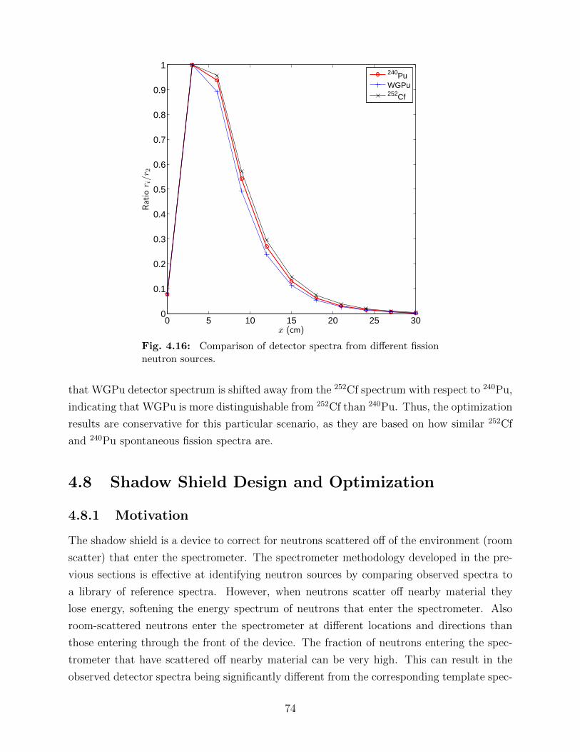
0 5 10 15 20 25 300
0.1
0.2
0.3
0.4
0.5
0.6
0.7
0.8
0.9
1
x (cm)
Ratio
r i/r 2
240PuWGPu252Cf
Fig. 4.16: Comparison of detector spectra from different fissionneutron sources.
that WGPu detector spectrum is shifted away from the 252Cf spectrum with respect to 240Pu,
indicating that WGPu is more distinguishable from 252Cf than 240Pu. Thus, the optimization
results are conservative for this particular scenario, as they are based on how similar 252Cf
and 240Pu spontaneous fission spectra are.
4.8 Shadow Shield Design and Optimization
4.8.1 Motivation
The shadow shield is a device to correct for neutrons scattered off of the environment (room
scatter) that enter the spectrometer. The spectrometer methodology developed in the pre-
vious sections is effective at identifying neutron sources by comparing observed spectra to
a library of reference spectra. However, when neutrons scatter off nearby material they
lose energy, softening the energy spectrum of neutrons that enter the spectrometer. Also
room-scattered neutrons enter the spectrometer at different locations and directions than
those entering through the front of the device. The fraction of neutrons entering the spec-
trometer that have scattered off nearby material can be very high. This can result in the
observed detector spectra being significantly different from the corresponding template spec-
74
tra (particularly in the first few detectors, which detect lower energy neutrons). For accurate
identification of sources in application, room-scatter effects must be corrected.
One solution to correct room-scatter neutrons is to account for room scatter in the tem-
plates. However, it would be difficult to develop a manageable number of templates that
covers the large variety of possible environments that could be encountered. Another ap-
proach would be to prevent room-scattered neutrons from entering the spectrometer. A layer
of Cd around the cylindrical and back surface of the spectrometer, followed by a layer of sev-
eral centimeters of HDPE would prevent the majority of neutrons from entering the side and
back of the device. Although this would provide some correction, the overall weight would
be significantly increased, and it would not account for room-scattered neutrons entering the
front of the device, an issue discussed further in Section 4.8.6.
The shadow shield provides an alternative method that accounts for room-scattered neu-
trons by taking two separate measurements. For the first measurement, the shadow shield
is placed between the source and the spectrometer. Ideally, the shield absorbs or deflects
all neutrons traveling directly from the source to the front of the device, masking the spec-
trometer from the line-of-sight (LOS) response. In the second measurement, the shield is
removed and the spectrometer measures the response from both the LOS and room-scattered
neutrons. Fig. 4.17 illustrates the two measurements, as well as possible neutron paths. Be-
cause the second measurement is a superposition of LOS and room-scattered neutrons, the
difference of the first measurement from the second results in the line of sight response (the
shadow of the shield). This net response is much closer to that of a void and can be used
to identify the source via comparison to templates from void simulations, eliminating de-
pendence on the environment. It is noted the counting time of these two measurements
is the same, with the neutron source and environment unchanged. Although taking two
separate measurements is not ideal in practice, it is no different than background measure-
ments required in the vast majority of radiation detection applications. Additionally, any
non-directional background source that is constant in time (such as cosmic neutrons or a
reactor) will be included in both measurements and thus eliminated from the net response.
Although bursts of spallation neutrons in Fe produced by cosmic background (known as the
“ship effect”) could be an issue, these can potentially be accounted for via temporal analysis
of the measurements, as discussed in Kouzes et al. [2007].
Shadow shields (typically referred to as shadow cones) are commonly used for precise
measurement of neutron energy spectra [ISO, 2000]. This section explores the utility of a
shadow shield and optimizes the design and implementation of the shield via MCNP simula-
tions. The procedure of identifying sources using FOM values is modified and demonstrated
for a variety of sources for the optimal shield design and location. The impact of different
75

Omni-directional Source
SpectrometerRemovable
Shield
B
A
x
L
D
C
Fig. 4.17: Illustration of the two shadow shield measurements. Several possible neutron pathsare illustrated: (A) neutrons deflected or absorbed in the shield, (B) neutrons scattered off of theenvironment entering the front of the spectrometer without interacting in the shield, (C line-of-siteneutrons, and (D) neutrons scattered off of the environment entering the front of the device.
76
types of rooms is briefly analyzed as well.
4.8.2 Source Identification with Shadow Shield Measurements
The difference in the detector spectra from the two shadow shield measurements described
in the previous section (referred to herein as the net spectra) are used to identify observed
sources by comparing the net spectra against templates created in a void using FOM values
as before. The equation for the FOM value of the j-th source is
FOM j =
Ndet∑i=1
(Ri − Sji )2
σ2(Ri) + σ2(Sji ). ((4.4))
The terms Ri and σ2(Ri) of the above equation are modified from the original definitions in
Section 4.1.2 to account for the two different shadow shield measurements. The value Ri is
the logarithm of the normalized difference in the two counting measurements, observed at
the i-th detector position, i.e.,
Ri = ln
(Cnsi − Cs
i
Cnsnorm − Cs
norm
), (4.29)
where the superscript ns indicates the observed counts with no shield present, the superscript
s is the observed counts with the shield in place, and the subscript norm indicates the chosen
normalization detector position. The uncertainty term, σ2(Ri), is by definition
σ2(Ri) = σ2
[ln
(Cnsi − Cs
i
Cnsnorm − Cs
norm
)]. (4.30)
Application of the error propagation formula (Eq. (2.27)) to the term in brackets reduces
the above equation to
σ2(Ri) =(Cns
i + Csi )
(Cnsi − Cs
i )2
+(Cns
norm + Csnorm)
(Cnsnorm − Cs
norm)2. (4.31)
There are no changes required to the template values Si to account for room scatter,
except that the templates are generated using an isotropic point source; template simulations
are still performed with the spectrometer and source present in a void. Tallies from void
simulations are labeled with the superscript void. Values of FOM calculated using the
modified definitions given above are referred to as FOMroom throughout this section for
clarity.
77
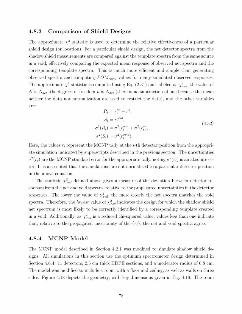
4.8.3 Comparison of Shield Designs
The approximate χ2 statistic is used to determine the relative effectiveness of a particular
shield design (or location). For a particular shield design, the net detector spectra from the
shadow shield measurements are compared against the template spectra from the same source
in a void, effectively comparing the expected mean response of observed net spectra and the
corresponding template spectra. This is much more efficient and simple than generating
observed spectra and computing FOMroom values for many simulated observed responses.
The approximate χ2 statistic is computed using Eq. (2.31) and labeled as χ2red; the value of
N is Ndet, the degrees of freedom µ is Ndet (there is no subtraction of one because the mean
neither the data nor normalization are used to restrict the data), and the other variables
are:Ri = rnsi − rs,Si = rvoidi ,
σ2(Ri) = σ2(rnsi ) + σ2(rsi ),
σ2(Si) = σ2(rvoidi ).
(4.32)
Here, the values ri represent the MCNP tally at the i-th detector position from the appropri-
ate simulation indicated by superscripts described in the previous section. The uncertainties
σ2(ri) are the MCNP standard error for the appropriate tally, noting σ2(ri) is an absolute er-
ror. It is also noted that the simulations are not normalized to a particular detector position
in the above equation.
The statistic χ2red defined above gives a measure of the deviation between detector re-
sponses from the net and void spectra, relative to the propagated uncertainties in the detector
responses. The lower the value of χ2red, the more closely the net spectra matches the void
spectra. Therefore, the lowest value of χ2red indicates the design for which the shadow shield
net spectrum is most likely to be correctly identified by a corresponding template created
in a void. Additionally, as χ2red is a reduced chi-squared value, values less than one indicate
that, relative to the propagated uncertainty of the ri, the net and void spectra agree.
4.8.4 MCNP Model
The MCNP model described in Section 4.2.1 was modified to simulate shadow shield de-
signs. All simulations in this section use the optimum spectrometer design determined in
Section 4.6.4: 11 detectors, 2.5 cm thick HDPE sections, and a moderator radius of 6.8 cm.
The model was modified to include a room with a floor and ceiling, as well as walls on three
sides. Figure 4.18 depicts the geometry, with key dimensions given in Fig. 4.19. The room
78
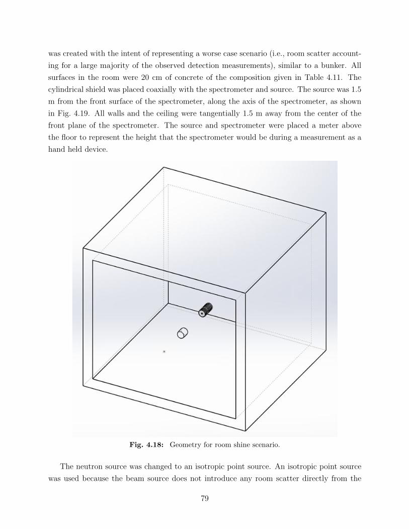
was created with the intent of representing a worse case scenario (i.e., room scatter account-
ing for a large majority of the observed detection measurements), similar to a bunker. All
surfaces in the room were 20 cm of concrete of the composition given in Table 4.11. The
cylindrical shield was placed coaxially with the spectrometer and source. The source was 1.5
m from the front surface of the spectrometer, along the axis of the spectrometer, as shown
in Fig. 4.19. All walls and the ceiling were tangentially 1.5 m away from the center of the
front plane of the spectrometer. The source and spectrometer were placed a meter above
the floor to represent the height that the spectrometer would be during a measurement as a
hand held device.
Fig. 4.18: Geometry for room shine scenario.
The neutron source was changed to an isotropic point source. An isotropic point source
was used because the beam source does not introduce any room scatter directly from the
79
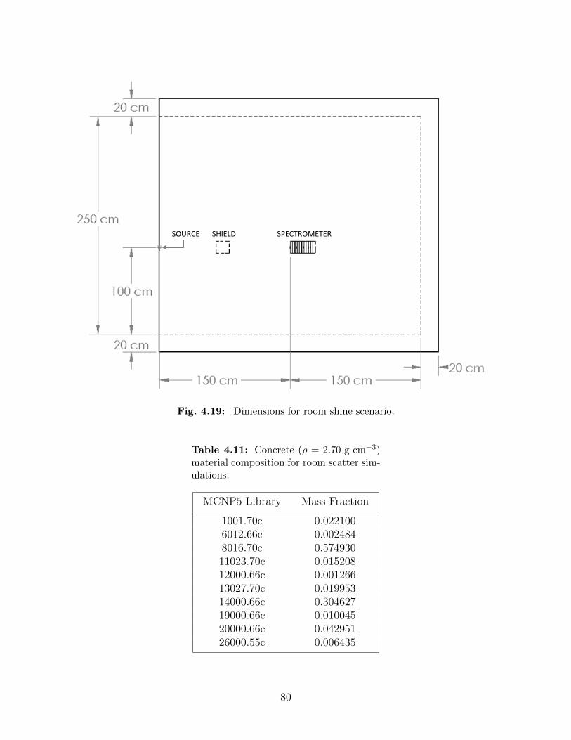
SOURCE SHIELD SPECTROMETER
Fig. 4.19: Dimensions for room shine scenario.
Table 4.11: Concrete (ρ = 2.70 g cm−3)material composition for room scatter sim-ulations.
MCNP5 Library Mass Fraction
1001.70c 0.0221006012.66c 0.0024848016.70c 0.57493011023.70c 0.01520812000.66c 0.00126613027.70c 0.01995314000.66c 0.30462719000.66c 0.01004520000.66c 0.04295126000.55c 0.006435
80
source. Also, fewer histories are required to reduce the variance for a point than a disk
source. The reduced number of histories was of particular interest for the simulations with
the shadow shield in place because the shield prevents the majority of neutron histories from
reaching the tallies. The directional source biasing variance reduction method described in
Section 2.3.2 was used. Particles were only created in direction cosines between 0 and 1,
as measured from the central axis of the spectrometer and source. It is noted that here,
because the source is a point, and room scatter is modeled, the tally per source particle is
different than the rally per incident neutron on the device, unlike that in the previous beam
source simulations.
To simulate the two shadow shield measurements, two simulations were performed. One
with the shield in place, and another with the shield removed (the cells are replaced by a void
in the model). The shield is of a cylindrical shape the same diameter as the spectrometer.
The cylindrical shield’s central axis is colinear with the axis of the spectrometer and source.
It is noted that typically shadow shields are referred to as a shadow cone, because the shape
is usually tapered towards the source [ISO, 2000]. The tapering is to prevent as little room
scatter from the source from being shielded, while still blocking the entire LOS response.
This geometry is not used here to help eliminate human error in lining up the shield in
application.
The room scatter simulations are very inefficient computationally because many neutrons
are terminated in the shield, and scattered neutrons have to go through multiple scatters
in the room to reach the source; these effects lead to poor convergence. To limit the total
number of simulations, a single neutron source was used for optimizing shield thickness and
location. The 30-cm D20 moderated 252Cf neutron source from Table 4.1 (252Cf - D2O )
was chosen. The 252Cf - D2O source features a relatively strong epithermal energy neutron
source, as well as covering the energy range of fast neutrons seen in the majority of neutron
sources. The epithermal and lower energy neutrons are of particular interest when analyzing
the room-scatter scenario because neutrons with low numbers of scatters in the room are the
most likely to reach the first and last few detectors, where the biggest deviation from void
templates is seen.
For optimization of shield thickness, an additional simulation was performed with the
shadow shield and spectrometer in a void to determine the probability LOS neutrons escape
the shield. A parallel uniform neutron beam of the same diameter as the shield was used.
Parallel incident neutrons represent the highest probability of escaping the shield. An F1
tally, labeled as Jshield, was used on the front surface of the spectrometer to determine the
probability, per source neutron, that a neutron escapes the shield and enters the spectrom-
eter. An F1 tally determines the number of neutrons that cross a surface in any direction,
81
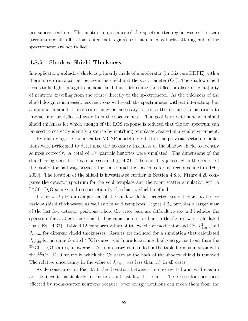
per source neutron. The neutron importance of the spectrometer region was set to zero
(terminating all tallies that enter that region) so that neutrons backscattering out of the
spectrometer are not tallied.
4.8.5 Shadow Shield Thickness
In application, a shadow shield is primarily made of a moderator (in this case HDPE) with a
thermal neutron absorber between the shield and the spectrometer (Cd). The shadow shield
needs to be light enough to be hand-held, but thick enough to deflect or absorb the majority
of neutrons traveling from the source directly to the spectrometer. As the thickness of the
shield design is increased, less neutrons will reach the spectrometer without interacting, but
a minimal amount of moderator may be necessary to cause the majority of neutrons to
interact and be deflected away from the spectrometer. The goal is to determine a minimal
shield thickness for which enough of the LOS response is reduced that the net spectrum can
be used to correctly identify a source by matching templates created in a void environment.
By modifying the room-scatter MCNP model described in the previous section, simula-
tions were performed to determine the necessary thickness of the shadow shield to identify
sources correctly. A total of 109 particle histories were simulated. The dimensions of the
shield being considered can be seen in Fig. 4.21. The shield is placed with the center of
the moderator half way between the source and the spectrometer, as recommended in [ISO,
2000]. The location of the shield is investigated further in Section 4.8.6. Figure 4.20 com-
pares the detector spectrum for the void template and the room scatter simulation with a252Cf - D2O source and no correction by the shadow shield method.
Figure 4.22 plots a comparison of the shadow shield corrected net detector spectra for
various shield thicknesses, as well as the void templates; Figure 4.23 provides a larger view
of the last few detector positions where the error bars are difficult to see and includes the
spectrum for a 20-cm thick shield. The values and error bars in the figures were calculated
using Eq. (4.32). Table 4.12 compares values of the weight of moderator and Cd, χ2red , and
Jshield for different shield thicknesses. Results are included for a simulation that calculated
Jshield for an unmoderated 252Cf source, which produces more high-energy neutrons than the252Cf - D2O source, on average. Also, an entry is included in the table for a simulation with
the 252Cf - D2O source in which the Cd sheet at the back of the shadow shield is removed
The relative uncertainty in the value of Jshield was less than 1% in all cases.
As demonstrated in Fig. 4.20, the deviation between the uncorrected and void spectra
are significant, particularly in the first and last few detectors. These detectors are most
affected by room-scatter neutrons because lower energy neutrons can reach them from the
82
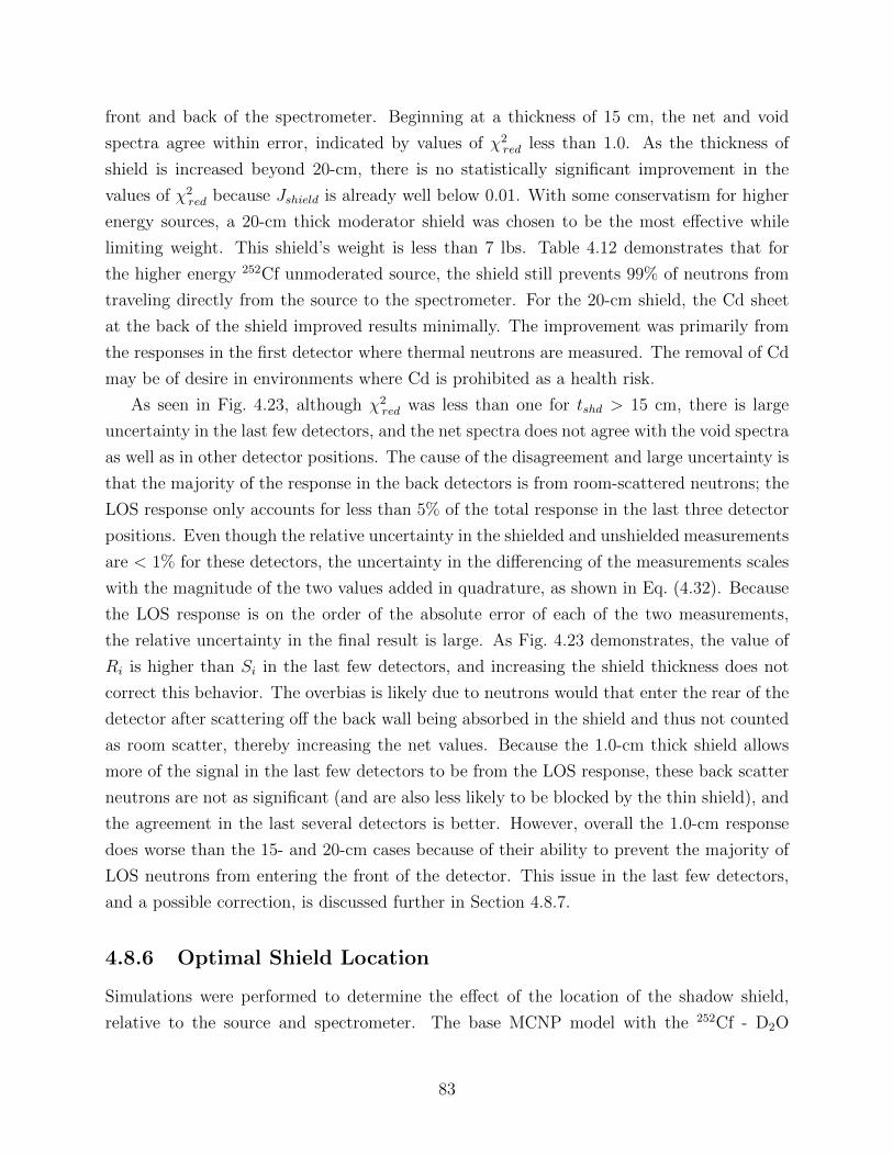
front and back of the spectrometer. Beginning at a thickness of 15 cm, the net and void
spectra agree within error, indicated by values of χ2red less than 1.0. As the thickness of
shield is increased beyond 20-cm, there is no statistically significant improvement in the
values of χ2red because Jshield is already well below 0.01. With some conservatism for higher
energy sources, a 20-cm thick moderator shield was chosen to be the most effective while
limiting weight. This shield’s weight is less than 7 lbs. Table 4.12 demonstrates that for
the higher energy 252Cf unmoderated source, the shield still prevents 99% of neutrons from
traveling directly from the source to the spectrometer. For the 20-cm shield, the Cd sheet
at the back of the shield improved results minimally. The improvement was primarily from
the responses in the first detector where thermal neutrons are measured. The removal of Cd
may be of desire in environments where Cd is prohibited as a health risk.
As seen in Fig. 4.23, although χ2red was less than one for tshd > 15 cm, there is large
uncertainty in the last few detectors, and the net spectra does not agree with the void spectra
as well as in other detector positions. The cause of the disagreement and large uncertainty is
that the majority of the response in the back detectors is from room-scattered neutrons; the
LOS response only accounts for less than 5% of the total response in the last three detector
positions. Even though the relative uncertainty in the shielded and unshielded measurements
are < 1% for these detectors, the uncertainty in the differencing of the measurements scales
with the magnitude of the two values added in quadrature, as shown in Eq. (4.32). Because
the LOS response is on the order of the absolute error of each of the two measurements,
the relative uncertainty in the final result is large. As Fig. 4.23 demonstrates, the value of
Ri is higher than Si in the last few detectors, and increasing the shield thickness does not
correct this behavior. The overbias is likely due to neutrons would that enter the rear of the
detector after scattering off the back wall being absorbed in the shield and thus not counted
as room scatter, thereby increasing the net values. Because the 1.0-cm thick shield allows
more of the signal in the last few detectors to be from the LOS response, these back scatter
neutrons are not as significant (and are also less likely to be blocked by the thin shield), and
the agreement in the last several detectors is better. However, overall the 1.0-cm response
does worse than the 15- and 20-cm cases because of their ability to prevent the majority of
LOS neutrons from entering the front of the detector. This issue in the last few detectors,
and a possible correction, is discussed further in Section 4.8.7.
4.8.6 Optimal Shield Location
Simulations were performed to determine the effect of the location of the shadow shield,
relative to the source and spectrometer. The base MCNP model with the 252Cf - D2O
83
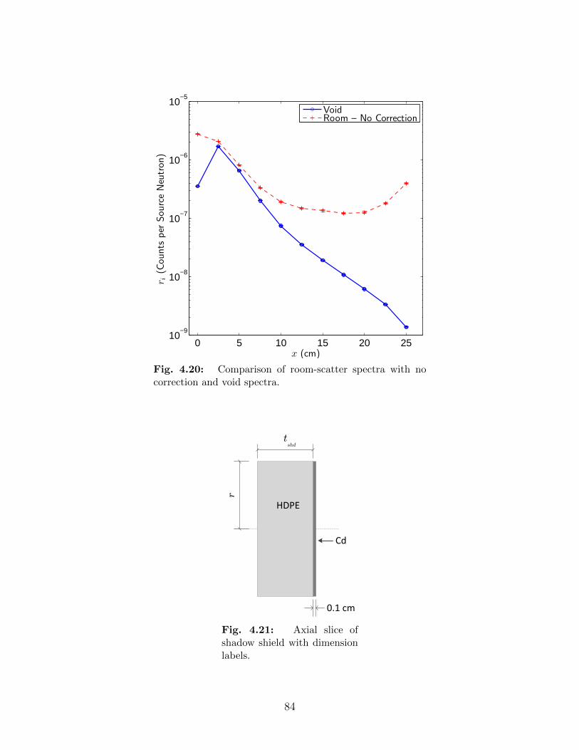
0 5 10 15 20 2510
−9
10−8
10−7
10−6
10−5
x (cm)
r i(Counts
per
SourceNeutron)
VoidRoom – No Correction
Fig. 4.20: Comparison of room-scatter spectra with nocorrection and void spectra.
HDPE
Cd
t
shd
r
0.1 cm
Fig. 4.21: Axial slice ofshadow shield with dimensionlabels.
84
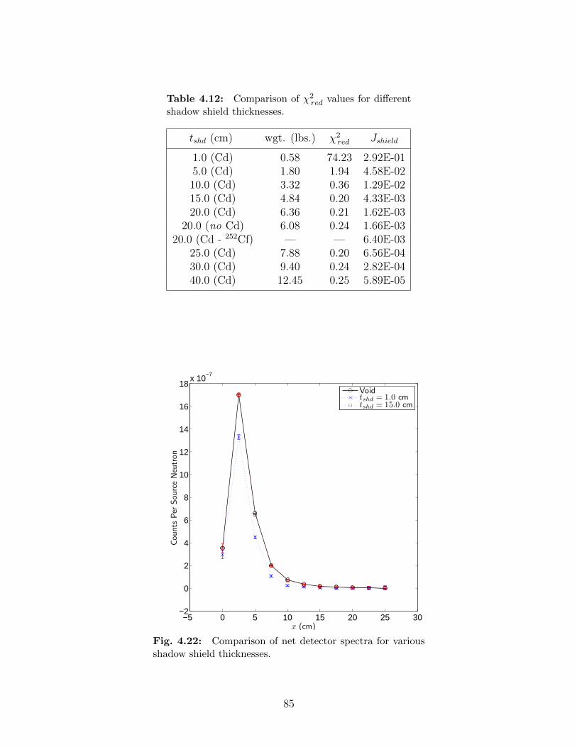
Table 4.12: Comparison of χ2red values for different
shadow shield thicknesses.
tshd (cm) wgt. (lbs.) χ2red Jshield
1.0 (Cd) 0.58 74.23 2.92E-015.0 (Cd) 1.80 1.94 4.58E-0210.0 (Cd) 3.32 0.36 1.29E-0215.0 (Cd) 4.84 0.20 4.33E-0320.0 (Cd) 6.36 0.21 1.62E-03
20.0 (no Cd) 6.08 0.24 1.66E-0320.0 (Cd - 252Cf) — — 6.40E-03
25.0 (Cd) 7.88 0.20 6.56E-0430.0 (Cd) 9.40 0.24 2.82E-0440.0 (Cd) 12.45 0.25 5.89E-05
−5 0 5 10 15 20 25 30−2
0
2
4
6
8
10
12
14
16
18x 10
−7
Counts
Per
SourceNeutron
x (cm)
Voidtshd = 1.0 cmtshd = 15.0 cm
Fig. 4.22: Comparison of net detector spectra for variousshadow shield thicknesses.
85
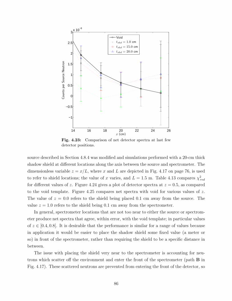
14 16 18 20 22 24 26
−1
−0.5
0
0.5
1
1.5
2
2.5
3x 10
−8
Counts
per
SourceNeutron
x (cm)
Void
tshd = 1.0 cm
tshd = 15.0 cm
tshd = 20.0 cm
Fig. 4.23: Comparison of net detector spectra at last fewdetector positions.
source described in Section 4.8.4 was modified and simulations performed with a 20-cm thick
shadow shield at different locations along the axis between the source and spectrometer. The
dimensionless variable z = x/L, where x and L are depicted in Fig. 4.17 on page 76, is used
to refer to shield locations; the value of x varies, and L = 1.5 m. Table 4.13 compares χ2red
for different values of z. Figure 4.24 gives a plot of detector spectra at z = 0.5, as compared
to the void template. Figure 4.25 compares net spectra with void for various values of z.
The value of z = 0.0 refers to the shield being placed 0.1 cm away from the source. The
value z = 1.0 refers to the shield being 0.1 cm away from the spectrometer.
In general, spectrometer locations that are not too near to either the source or spectrom-
eter produce net spectra that agree, within error, with the void template; in particular values
of z ∈ [0.4, 0.8]. It is desirable that the performance is similar for a range of values because
in application it would be easier to place the shadow shield some fixed value (a meter or
so) in front of the spectrometer, rather than requiring the shield to be a specific distance in
between.
The issue with placing the shield very near to the spectrometer is accounting for neu-
trons which scatter off the environment and enter the front of the spectrometer (path B in
Fig. 4.17). These scattered neutrons are prevented from entering the front of the detector, so
86
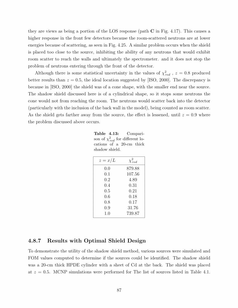
they are views as being a portion of the LOS response (path C in Fig. 4.17). This causes a
higher response in the front few detectors because the room-scattered neutrons are at lower
energies because of scattering, as seen in Fig. 4.25. A similar problem occurs when the shield
is placed too close to the source, inhibiting the ability of any neutrons that would exhibit
room scatter to reach the walls and ultimately the spectrometer. and it does not stop the
problem of neutrons entering through the front of the detector.
Although there is some statistical uncertainty in the values of χ2red , z = 0.8 produced
better results than z = 0.5, the ideal location suggested by [ISO, 2000]. The discrepancy is
because in [ISO, 2000] the shield was of a cone shape, with the smaller end near the source.
The shadow shield discussed here is of a cylindrical shape, so it stops some neutrons the
cone would not from reaching the room. The neutrons would scatter back into the detector
(particularly with the inclusion of the back wall in the model), being counted as room scatter.
As the shield gets farther away from the source, the effect is lessened, until z = 0.9 where
the problem discussed above occurs.
Table 4.13: Compari-son of χ2
red for different lo-cations of a 20-cm thickshadow shield.
z = x/L χ2red
0.0 879.880.1 107.560.2 4.890.4 0.310.5 0.210.6 0.180.8 0.170.9 31.761.0 739.87
4.8.7 Results with Optimal Shield Design
To demonstrate the utility of the shadow shield method, various sources were simulated and
FOM values computed to determine if the sources could be identified. The shadow shield
was a 20-cm thick HPDE cylinder with a sheet of Cd at the back. The shield was placed
at z = 0.5. MCNP simulations were performed for The list of sources listed in Table 4.1.
87
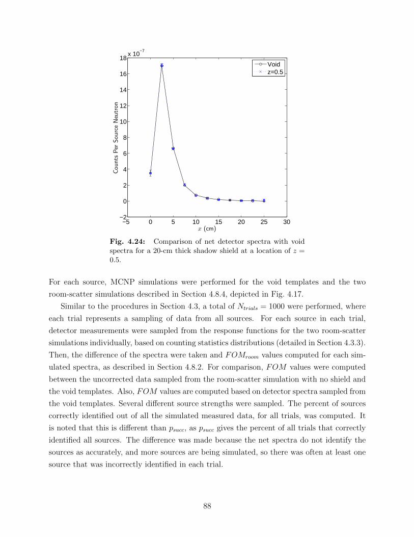
−5 0 5 10 15 20 25 30−2
0
2
4
6
8
10
12
14
16
18x 10
−7
Counts
Per
SourceNeutron
x (cm)
Voidz=0.5
Fig. 4.24: Comparison of net detector spectra with voidspectra for a 20-cm thick shadow shield at a location of z =0.5.
For each source, MCNP simulations were performed for the void templates and the two
room-scatter simulations described in Section 4.8.4, depicted in Fig. 4.17.
Similar to the procedures in Section 4.3, a total of Ntrials = 1000 were performed, where
each trial represents a sampling of data from all sources. For each source in each trial,
detector measurements were sampled from the response functions for the two room-scatter
simulations individually, based on counting statistics distributions (detailed in Section 4.3.3).
Then, the difference of the spectra were taken and FOMroom values computed for each sim-
ulated spectra, as described in Section 4.8.2. For comparison, FOM values were computed
between the uncorrected data sampled from the room-scatter simulation with no shield and
the void templates. Also, FOM values are computed based on detector spectra sampled from
the void templates. Several different source strengths were sampled. The percent of sources
correctly identified out of all the simulated measured data, for all trials, was computed. It
is noted that this is different than psucc, as psucc gives the percent of all trials that correctly
identified all sources. The difference was made because the net spectra do not identify the
sources as accurately, and more sources are being simulated, so there was often at least one
source that was incorrectly identified in each trial.
88
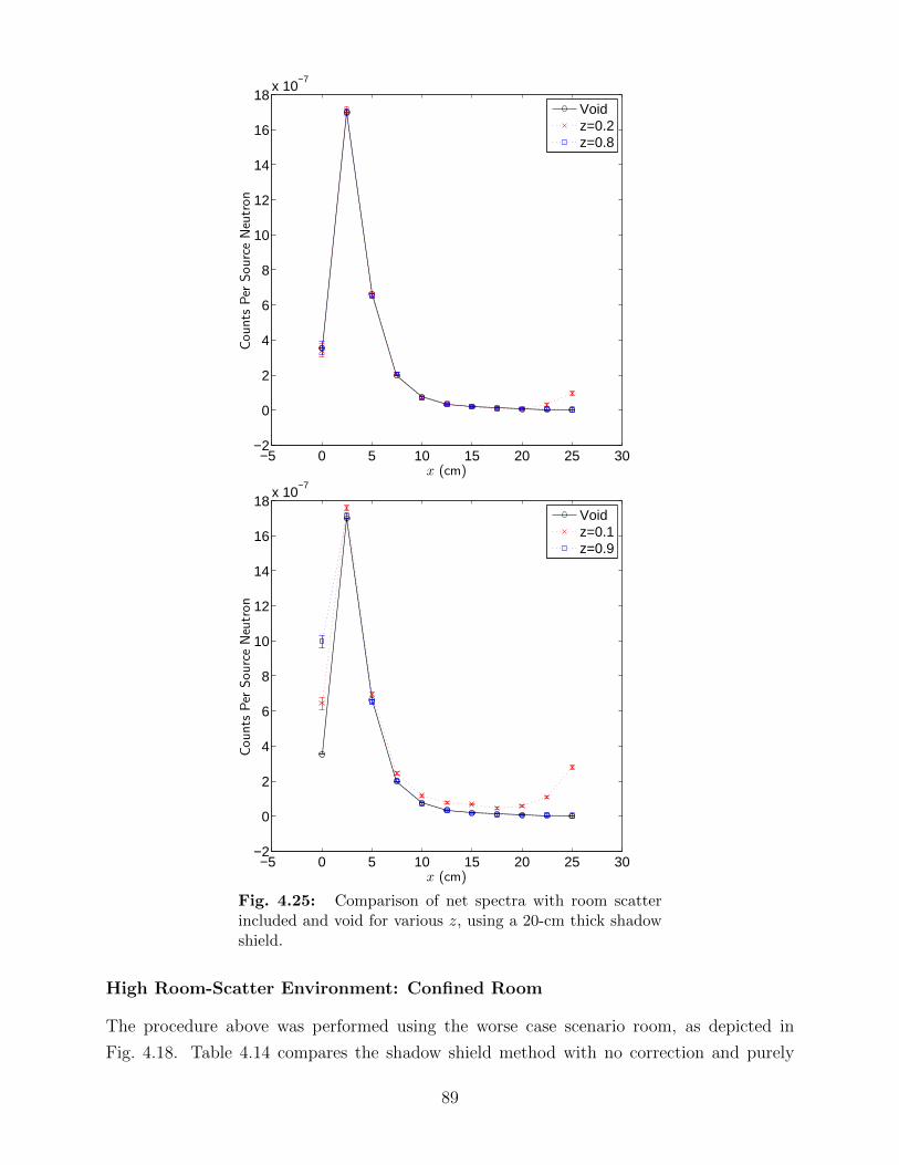
−5 0 5 10 15 20 25 30−2
0
2
4
6
8
10
12
14
16
18x 10
−7
Counts
Per
SourceNeutron
x (cm)
Voidz=0.2z=0.8
−5 0 5 10 15 20 25 30−2
0
2
4
6
8
10
12
14
16
18x 10
−7
x (cm)
Counts
Per
SourceNeutron
Voidz=0.1z=0.9
Fig. 4.25: Comparison of net spectra with room scatterincluded and void for various z, using a 20-cm thick shadowshield.
High Room-Scatter Environment: Confined Room
The procedure above was performed using the worse case scenario room, as depicted in
Fig. 4.18. Table 4.14 compares the shadow shield method with no correction and purely
89
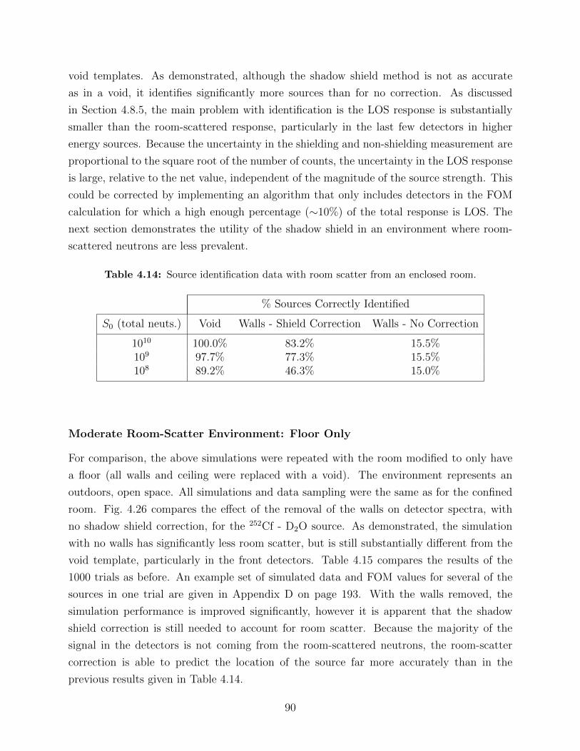
void templates. As demonstrated, although the shadow shield method is not as accurate
as in a void, it identifies significantly more sources than for no correction. As discussed
in Section 4.8.5, the main problem with identification is the LOS response is substantially
smaller than the room-scattered response, particularly in the last few detectors in higher
energy sources. Because the uncertainty in the shielding and non-shielding measurement are
proportional to the square root of the number of counts, the uncertainty in the LOS response
is large, relative to the net value, independent of the magnitude of the source strength. This
could be corrected by implementing an algorithm that only includes detectors in the FOM
calculation for which a high enough percentage (∼10%) of the total response is LOS. The
next section demonstrates the utility of the shadow shield in an environment where room-
scattered neutrons are less prevalent.
Table 4.14: Source identification data with room scatter from an enclosed room.
% Sources Correctly Identified
S0 (total neuts.) Void Walls - Shield Correction Walls - No Correction
1010 100.0% 83.2% 15.5%109 97.7% 77.3% 15.5%108 89.2% 46.3% 15.0%
Moderate Room-Scatter Environment: Floor Only
For comparison, the above simulations were repeated with the room modified to only have
a floor (all walls and ceiling were replaced with a void). The environment represents an
outdoors, open space. All simulations and data sampling were the same as for the confined
room. Fig. 4.26 compares the effect of the removal of the walls on detector spectra, with
no shadow shield correction, for the 252Cf - D2O source. As demonstrated, the simulation
with no walls has significantly less room scatter, but is still substantially different from the
void template, particularly in the front detectors. Table 4.15 compares the results of the
1000 trials as before. An example set of simulated data and FOM values for several of the
sources in one trial are given in Appendix D on page 193. With the walls removed, the
simulation performance is improved significantly, however it is apparent that the shadow
shield correction is still needed to account for room scatter. Because the majority of the
signal in the detectors is not coming from the room-scattered neutrons, the room-scatter
correction is able to predict the location of the source far more accurately than in the
previous results given in Table 4.14.
90
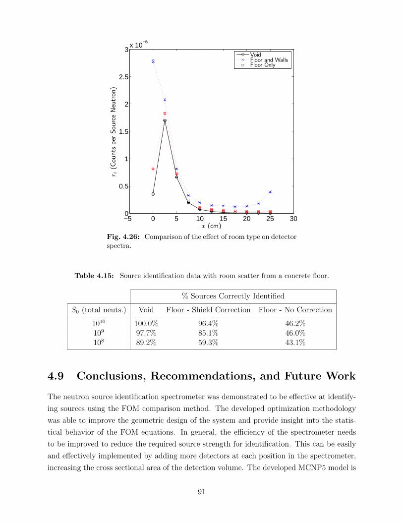
−5 0 5 10 15 20 25 300
0.5
1
1.5
2
2.5
3x 10
−6
r i(Counts
per
SourceNeutron)
x (cm)
VoidFloor and WallsFloor Only
Fig. 4.26: Comparison of the effect of room type on detectorspectra.
Table 4.15: Source identification data with room scatter from a concrete floor.
% Sources Correctly Identified
S0 (total neuts.) Void Floor - Shield Correction Floor - No Correction
1010 100.0% 96.4% 46.2%109 97.7% 85.1% 46.0%108 89.2% 59.3% 43.1%
4.9 Conclusions, Recommendations, and Future Work
The neutron source identification spectrometer was demonstrated to be effective at identify-
ing sources using the FOM comparison method. The developed optimization methodology
was able to improve the geometric design of the system and provide insight into the statis-
tical behavior of the FOM equations. In general, the efficiency of the spectrometer needs
to be improved to reduce the required source strength for identification. This can be easily
and effectively implemented by adding more detectors at each position in the spectrometer,
increasing the cross sectional area of the detection volume. The developed MCNP5 model is
91
in general accurate, but the fidelity can be improved by explicit modeling of the detectors in
MCNP6. For actual detection of spontaneous fission sources, which have very similar energy
spectra, templates should be generated from experimental data. For high energy neutron
sources, which will register counts at deeper detector positions, the front response should
not be included in FOM calculations. In general, the response of the first detector is not well
modeled by the MCNP5 artificial detector model. Additionally, most thermal neutrons are
actually from moderation through either room scatter or moderator surrounding the source,
so the first position would not match well to experiments. However, the front detector is
still very useful for identifying the presence of thermal neutron sources. The shadow shield
method is an effective method, except for cases with extremely low LOS signal.
A simple simulation study still to be investigated would be adjusting the way that the
algorithm accounts for detectors with low numbers of counts. The current algorithm con-
tributes scores to the FOM from detector positions with non-zero counts. If this cutoff is
raised from zero to a higher value, e.g., 20 then the FOM calculations would be improved,
as the low count rates are mostly just contributing statistical noise to FOM calculations.
Also, the effects on detector spectra from shielding and moderator placed around a neutron
source should be investigated.
A more important and involved study would be to determine the confidence intervals for
source identification. Although the relation of Θ and psucc provided some insight, the actual
distribution of the FOM values is unknown. Initial Monte Carlo studies demonstrate that
for the template that matches the source, FOM has a χ2(Ndet − 1) distribution, and the
error propagation estimate of σ(FOM) is very accurate. However, the distribution of the
FOM values for the incorrect templates are not χ2, and the estimate of σ(FOM) is very
poor, differing from the sample standard deviation by up to 150%. Additionally, in real
application, the templates will not match measured spectra perfectly because of differences
between reality and simulations. The differences would result in relatively large values of
FOMmin, i.e., the FOM for the correct template. Thus, confidence of identification based
on a χ2 distribution is unlikely, even for the correct source1. Future simulated data should
add some form of a random term into the simulated responses to account for detector noise
and modeling inaccuracies. Also, the inaccuracies in the estimated standard deviation can
be improved by removing the logarithms from the FOM, as the error propagation estimate
for logarithms is known to be very poor for large values [Taylor, 1997].
1The majority of FOMmin values would be relatively large and located in the region of the domain thatshould be the low-probability tail of a χ2(Ndet − 1) distribution [Hogg et al., 2013]. Thus, FOMmin wouldnot be distributed as χ2(Ndet − 1).
92

Chapter 5
Simulations of Neutron Multiplicity
Measurements with Perturbations to
Nuclear Data
5.1 Motivation
This chapter provides a summary of initial studies performed to analyze a known discrepancy
between multiplicity distributions generated by MCNP modeling and experimental data.
MCNP simulations have been known to demonstrate an overbias in multiplicity distributions
from a sphere of WGPu [Miller et al., 2010; Sood et al., 2011], and the cause of the overbias
is believed to be inaccuracies in the nuclear data, as demonstrated in Miller et al. [2010].
Perturbations were made to nuclear data for 239Pu ENDF/B-VII.1 data in ACE format to
attempt to correct the overbias.
Simulations of multiplicity and criticality experiments were performed to determine the
correction of overbias caused by the individual perturbations. The sets of resulting data
were compared using chi-squared analysis with the intent of reducing the bias in multiplicity
distributions without sacrificing the accuracy of keff in criticality experiments. Energy-
dependent perturbations to the mean of the total number of neutrons produced per fission,
ν, of 239Pu were analyzed. Also, energy-independent perturbations to microscopic neutron
capture, elastic scattering, and fission cross sections were performed. Several methods were
used to maintain realistic cross section relations from the original data. The main goal of
the cross section alterations is to determine how effective the perturbations are, relative to ν
alterations; if the cross section alterations are ineffective, then simulations of the multiplicity
experiments provide a useful tool for verifying tabulated ν data.
93
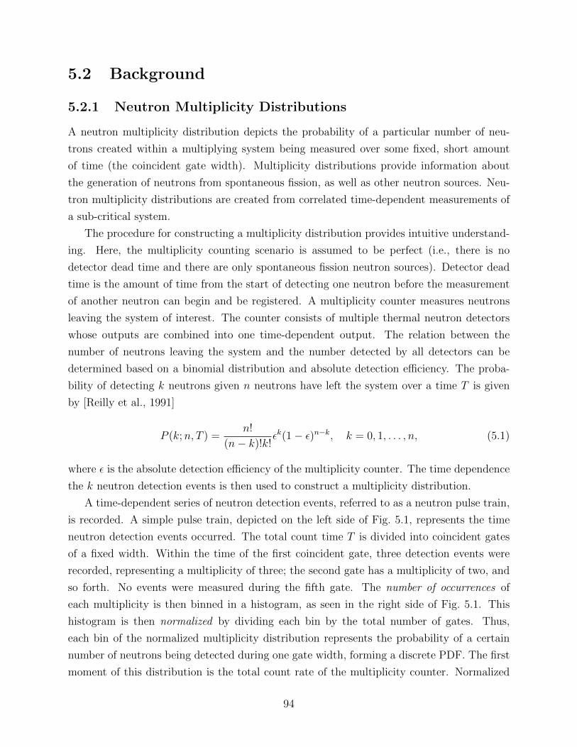
5.2 Background
5.2.1 Neutron Multiplicity Distributions
A neutron multiplicity distribution depicts the probability of a particular number of neu-
trons created within a multiplying system being measured over some fixed, short amount
of time (the coincident gate width). Multiplicity distributions provide information about
the generation of neutrons from spontaneous fission, as well as other neutron sources. Neu-
tron multiplicity distributions are created from correlated time-dependent measurements of
a sub-critical system.
The procedure for constructing a multiplicity distribution provides intuitive understand-
ing. Here, the multiplicity counting scenario is assumed to be perfect (i.e., there is no
detector dead time and there are only spontaneous fission neutron sources). Detector dead
time is the amount of time from the start of detecting one neutron before the measurement
of another neutron can begin and be registered. A multiplicity counter measures neutrons
leaving the system of interest. The counter consists of multiple thermal neutron detectors
whose outputs are combined into one time-dependent output. The relation between the
number of neutrons leaving the system and the number detected by all detectors can be
determined based on a binomial distribution and absolute detection efficiency. The proba-
bility of detecting k neutrons given n neutrons have left the system over a time T is given
by [Reilly et al., 1991]
P (k;n, T ) =n!
(n− k)!k!εk(1− ε)n−k, k = 0, 1, . . . , n, (5.1)
where ε is the absolute detection efficiency of the multiplicity counter. The time dependence
the k neutron detection events is then used to construct a multiplicity distribution.
A time-dependent series of neutron detection events, referred to as a neutron pulse train,
is recorded. A simple pulse train, depicted on the left side of Fig. 5.1, represents the time
neutron detection events occurred. The total count time T is divided into coincident gates
of a fixed width. Within the time of the first coincident gate, three detection events were
recorded, representing a multiplicity of three; the second gate has a multiplicity of two, and
so forth. No events were measured during the fifth gate. The number of occurrences of
each multiplicity is then binned in a histogram, as seen in the right side of Fig. 5.1. This
histogram is then normalized by dividing each bin by the total number of gates. Thus,
each bin of the normalized multiplicity distribution represents the probability of a certain
number of neutrons being detected during one gate width, forming a discrete PDF. The first
moment of this distribution is the total count rate of the multiplicity counter. Normalized
94
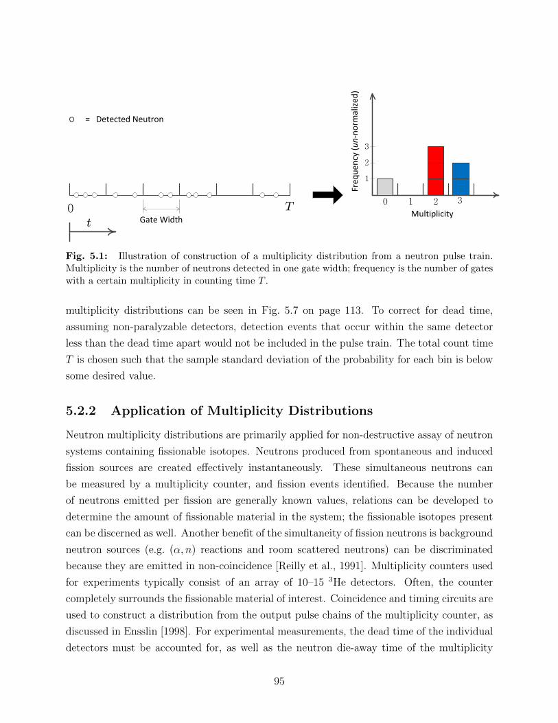
T
t
0Gate Width
Fre
qu
ency
(un
-no
rmal
ized
)
Multiplicity
0 1 2 3
= Detected Neutron
1
2
3
Fig. 5.1: Illustration of construction of a multiplicity distribution from a neutron pulse train.Multiplicity is the number of neutrons detected in one gate width; frequency is the number of gateswith a certain multiplicity in counting time T .
multiplicity distributions can be seen in Fig. 5.7 on page 113. To correct for dead time,
assuming non-paralyzable detectors, detection events that occur within the same detector
less than the dead time apart would not be included in the pulse train. The total count time
T is chosen such that the sample standard deviation of the probability for each bin is below
some desired value.
5.2.2 Application of Multiplicity Distributions
Neutron multiplicity distributions are primarily applied for non-destructive assay of neutron
systems containing fissionable isotopes. Neutrons produced from spontaneous and induced
fission sources are created effectively instantaneously. These simultaneous neutrons can
be measured by a multiplicity counter, and fission events identified. Because the number
of neutrons emitted per fission are generally known values, relations can be developed to
determine the amount of fissionable material in the system; the fissionable isotopes present
can be discerned as well. Another benefit of the simultaneity of fission neutrons is background
neutron sources (e.g. (α, n) reactions and room scattered neutrons) can be discriminated
because they are emitted in non-coincidence [Reilly et al., 1991]. Multiplicity counters used
for experiments typically consist of an array of 10–15 3He detectors. Often, the counter
completely surrounds the fissionable material of interest. Coincidence and timing circuits are
used to construct a distribution from the output pulse chains of the multiplicity counter, as
discussed in Ensslin [1998]. For experimental measurements, the dead time of the individual
detectors must be accounted for, as well as the neutron die-away time of the multiplicity
95
counter. The neutron die-away time is a time constant which describes the exponential decay
of a neutron population in a multiplicity counter over time because of the finite thermalization
and detection time of the device. Counter die-away and dead time are typically on the order
of a few µs, compared to gate widths, which are on the order of 1000 µs.
The theory relating a measured distribution to the multiplication properties of a fission-
able system has been applied since Feynman [1946], based on a simplified point model of
the system. Typically multiplicity counting analysis does not use the entire multiplicity dis-
tribution. Instead, the first three factorial moments of the distribution are used. The n-th
factorial moment of X is defined as E[X(X − 1)(X − 2) · · · (X − n + 1)]. In the case of
multiplicity distributions, X is the discreet random variable defined as the number of mea-
sured events in one gate. The factorial moments of the measured multiplicity distribution
are related to the moments of the spontaneous fission and induced fission rates of the system
that is being studied [Reilly et al., 1991]. The first moment of a measured multiplicity distri-
bution is the total neutron count rate. The second factorial moment (E[ν(ν−1)]) determines
the “doubles” rate. The doubles rate is the expected number of true coincident events of
two neutrons [Reilly et al., 1991], i.e., the rate that fission events releasing two neutrons
occur and are measured. The triples rate is similarly defined. Multiplicity distributions can
be misleading in that the measured multiplicities (the abscissa of the distribution) do not
represent true coincidence. The true coincidence of 3 neutrons in a sample is rare [Reilly
et al., 1991], even though multiplicities are much higher because there are many fission events
happening randomly throughout the sample.
Other distribution parameters of interest in measurements are the divergence of the ratio
of the variance to the mean from unity (unity is expected for a Poisson distribution), termed
the Feynman-Y statistic. The Feynman-Y can be related to the subcritical multiplication of
the system and used to verify the functionality of a multiplicity counter, as discussed in Croft
et al. [2012]. The relations of factorial moments and other statistics to the fission rates of
the system being measured are complex and beyond the scope and application of this work,
but the relations are derived and explained in Ensslin [1998]. In this chapter, multiplicity
distributions are used as a measure of subcritical multiplication, rather than to determine
spontaneous fission rates, doubles rates, etc.
96
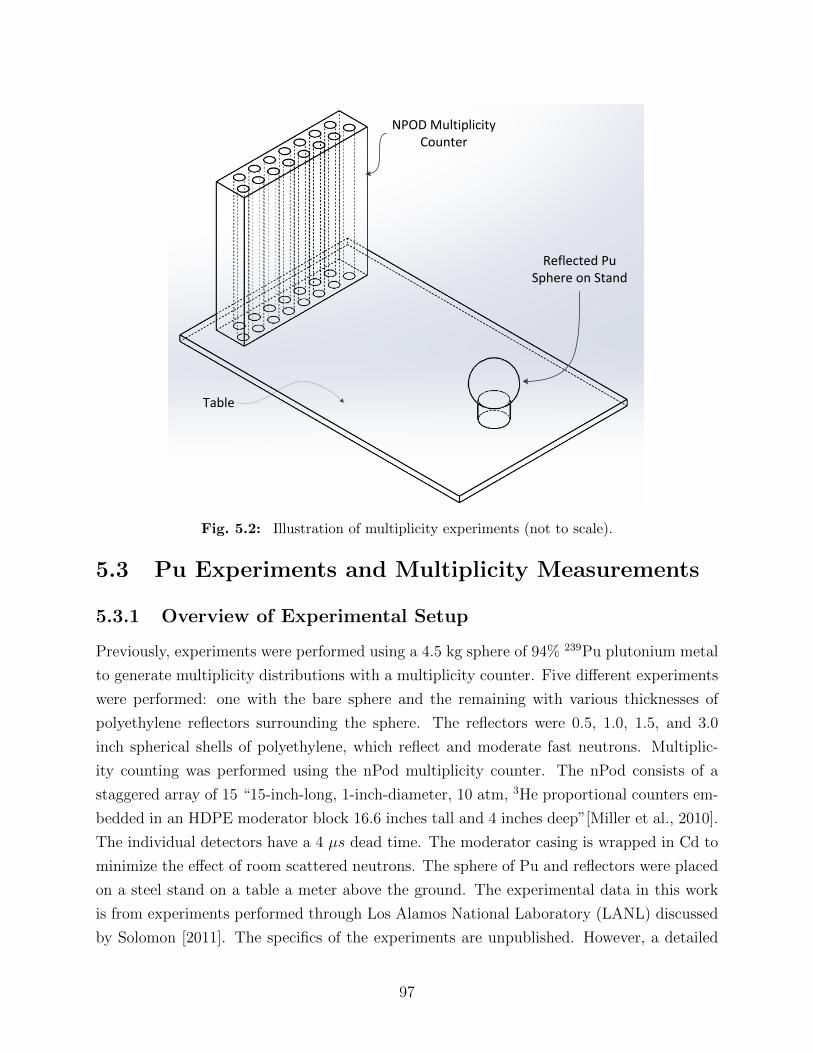
NPOD Multiplicity Counter
Table
Reflected Pu Sphere on Stand
Fig. 5.2: Illustration of multiplicity experiments (not to scale).
5.3 Pu Experiments and Multiplicity Measurements
5.3.1 Overview of Experimental Setup
Previously, experiments were performed using a 4.5 kg sphere of 94% 239Pu plutonium metal
to generate multiplicity distributions with a multiplicity counter. Five different experiments
were performed: one with the bare sphere and the remaining with various thicknesses of
polyethylene reflectors surrounding the sphere. The reflectors were 0.5, 1.0, 1.5, and 3.0
inch spherical shells of polyethylene, which reflect and moderate fast neutrons. Multiplic-
ity counting was performed using the nPod multiplicity counter. The nPod consists of a
staggered array of 15 “15-inch-long, 1-inch-diameter, 10 atm, 3He proportional counters em-
bedded in an HDPE moderator block 16.6 inches tall and 4 inches deep”[Miller et al., 2010].
The individual detectors have a 4 µs dead time. The moderator casing is wrapped in Cd to
minimize the effect of room scattered neutrons. The sphere of Pu and reflectors were placed
on a steel stand on a table a meter above the ground. The experimental data in this work
is from experiments performed through Los Alamos National Laboratory (LANL) discussed
by Solomon [2011]. The specifics of the experiments are unpublished. However, a detailed
97
explanation of experiments very similar to the experiments used in this work can be found
in [Mattingly, 2009]; the article discusses corrections to account for dead time and other
factors, as well as the use of multiplicity factorial moments to validate the experiments. The
primary difference between the experiments studied in this work (and by Solomon [2011])
and [Mattingly, 2009] is the reflector thicknesses. Another difference is the design of the
stands that the Pu spheres are placed on. The experimental multiplicity distributions and
their estimated statistical uncertainties are of high accuracy and validity in both cases, and
separate modeling of the systems demonstrate similar results. A diagram from an MCNP
model of the experiments in this work is given in Fig. 5.2. A SNAP-3 total neutron counter
is modeled as well (not pictured). This detector was used to verify that the simulated source
is accurate. Details on the SNAP-3 detector can be found in [Mattingly, 2009].
5.3.2 Previous Modeling Work
The LANL multiplicity experiments described above were previously modeled in a modified
version of MCNP5 with a multiplication patch, MCNP5 mult [Sood et al., 2011; Solomon,
2011]. The patch allows sampling of spontaneous fission source events and produces list-
mode tallies that provide time-dependent tally data. The detector geometry was modeled
explicitly and the list-mode tallies can provide the number of absorptions that have occured,
as well as when each absorption occured. The time-dependent tally data from the simulated
multiplicity-counter detector array are used to reconstruct multiplicity distributions with
the mtool.pl script. The mtool.pl script (used for work in Solomon [2011]) is a Perl script
which takes the time-dependent tallies from the MCNP list-mode tallies and constructs a
multiplicity distribution using a non-paralyzable dead-time correction. The non-paralyzable
dead-time correction is such that if multiple events occur within the dead time interval, only
one event is counted. This is alternative to a paralyzable dead-time correction where a second
event occurring resets the dead time window, allowing the detector to become completely
paralyzed. Previous studies using this MCNP5 model found that MCNP simulations predict
the mean and variance of the multiplicity distributions to be significantly larger values than
the multiplicity experiments [Miller et al., 2010; Solomon, 2011]. However, simulations were
able to accurately predict multiplicity distributions for a 252Cf source. The overbias was
found to worsen as the amount of multiplication in the system was increased by surrounding
the sphere with more polyethylene. A comparison of the experimental and MCNP5 mult
generated multiplicity distributions1 can be seen in Fig. 5.7 on page 113.
1The measured and simulated multiplicity distributions throughout this work are normalized. The verticalaxes are labeled as “Frequency”, referring to the probability of occurrence per multiplicity bin, i.e., therelative frequency, rather than the number of occurrences. Multiplicity bins are labeled as “Multiplets”.
98
Work has been done to determine the cause and magnitude of the overbias in MCNP using
MCNP PoliMi by [Miller et al., 2010], as well as from internal LANL analysis [Solomon,
2011; Sood et al., 2011]. Sensitivity studies on physical parameters were explored: diameter
of device, dead time, 239Pu mass density, etc. Previous results demonstrated that the bias
can be reduced by modifying the value of ν directly in the induced fission sampling routines
by Miller et al. [2010]; this effectively changes the energy-averaged value of ν by reducing all
of the tabular ν data by the same fraction. As a consequence, the computed values of keff
for simulations using the shifted ν data are very inaccurate. Because the MCNP bias over
experimental data increases with the amount of surrounding moderator, an energy-dependent
alteration of ν should reduce the bias more effectively. Additionally, it is known that the ν
data tend to be artificially high below 1.5 MeV [Chadwick et al., 2006]. In order to match
the JEZEBEL fast critical experiment [ICSBEP Handbook, 2004], ν values were increased
in the ENDF/B-VII.1 nuclear data. Below 1.5 MeV, ν tends to lie around two standard
deviations above the experimental data, as determined by covariance analysis by Chadwick
et al. [2006].
5.4 Methodology
5.4.1 Modifying Nuclear Data Files
In this work, the nuclear data read by MCNP5 mult was modified. The United States
Cross Section Evaluation Working Group is a collective group across many universities
and national laboratories which maintains nuclear data. In particular, they manage the
Evaluated Nuclear Data Files (ENDF) library. The current release of the ENDF library is
ENDF/B-VII.1 [Chadwick et al., 2006], where VII.1 is the version and B indicates the release
recommended for use (other versions contain non-verified data). The ENDF libraries con-
tain all cross sections and other tabulated nuclear data needed to perform most Monte Carlo
radiation transport simulations. The VII.1 release also contains experimentally-determined
covariance matrices, in many arbitrary formats, for neutron cross section and ν data.
The code MCNP5 reads data from “A Compact ENDF” (ACE) format files. The ACE
format files contain large arrays of numbers, typically organized by energy data points and
the value of the nuclear data of interest at that energy. Different portions of the nuclear
data are indexed by chains of pointers and numerical flags, whose meanings are given in Vol.
III of the MCNP manual [X-5 Monte Carlo Team, 2003]. Covariance data are only present
in the ENDF format. The covariance data of interest in this work are, in general, organized
as relative covariance terms, averaged over an energy group, divided into sub-matrices by
99
energy. However, the specific formats vary greatly.
The Nuclear Data Verification & Validation (NDVV) Python modules available at LANL
were used and expanded for reading and modifying nuclear data, with the intent of being
versatile enough to be applicable to other covariance data analyses. As the NDVV tools
are large codes, only newly created modules that are specifically relevant to the results in
this work are given. The modules added to NDVV for handling ENDF covariance matrices
in this work are the mf33.py and cov matrices.py modules. The ENDF format manual
can be used to understand the behaviour of these files. All ACE data are handled using the
ace sb.py module written for this work. These Python modules can be found in Appendix E,
with description on page 197.
5.4.2 Correlated Random Sampling of ν in ACE Files
Unique sets of correlated random ν data were used instead of employing a linear opti-
mization or some subjective method. The methods discussed in Section 2.1.7 were used to
sample correlated random values from covariance data. Both the Cholesky and eigenvalue
decomposition methods, with optional correction for non-positive-semidefinite matrices were
implemented. The decompositions were implemented using prebuilt Python linear algebra
models with PyLab, a modified version of Python; open-source documentation is available
at <www.scipy.org/PyLab>.
A small perturbation to ν data can have a large effect on results because the many fission-
based neutron multiplications that potentially take place throughout a single history. These
multiplications result in a non-linear change in results with respect to ν perturbations. A
linear optimization problem would likely get stuck in a local minima. Additionally, because
the problem was under-constrained (50 variables with only 6 sets of results), it is likely
a standard step-descent method (e.g. as gradient descent [Press et al., 1992]) would find
a minima that is not physically realistic. Using a covariance matrix to sample data adds
statistical confinement to potential values of the data, but requires some form of random
sampling of the space.
The covariance data used to correlate the randomly sampled numbers was read from the239Pu ENDF/B-VII.1 data library1. The library that was used to compile the ACE libraries
used in this work was ENDF/BVII.0. However, ENDF/B-VII.1 possesses the same values for
ν and all neutron cross sections as ENDF/B-VII.0 for 239Pu. The ν data for 239Pu contain
one row (and symmetric column) in the covariance matrix with all zeros. To handle this, the
1For some nuclear data, the ENDF/B-VII.1 covariance data contain co-relation terms between differentdata types and isotopes, for different energy groups. Only co-relation terms between energy groups, for aparticular type of nuclear data of 239Pu, are considered in this work.
100
submatrix of the correlation matrix with the row and column of zeros absent was used for
the decomposition and sampling process. Because there is no information on the variance
for that row, that sampled value is taken as the original value. For ν of 239Pu, below thermal
energies there is no covariance data.
The covariance matrix for ν data of 239Pu is positive definite and the Cholesky decompo-
sition was used. The covariance data are given as averages over certain energy groups. The
ν data are evaluated at certain energies for which linear interpolation is applied in between
to evaluate ν during simulations [ENDF-6 Manual, 2011]. There are also more energies for
which ν is evaluated than corresponding covariance energy groups. To map the sampled
covariance data to the ν data points, ν data was sampled as
ν ′(E) = σrel(Eg)ν(E)R(Eg) + ν(E). (5.2)
Here, ν(E) is the original value of ν at energy E, ν ′(E) is the perturbed ν data, Eg is
the covariance energy group that E lies in, σrel(Eg) is the relative standard deviation in
group Eg, and R(Eg) is the correlated standard normal random sample in group Eg as
described in Eq. (2.21) on page 12. The standard-normal-distributed random numbers were
generated using pre-built Python routines, which utilize the Mersenne Twister algorithm
and allows for specification of the random number generator state through a numerical
seed. Details on the sampling algorithms can be found in the open-source documentation at
<www.python.org/doc>
Observation on Sampling Correlation Matrix
The sampling method described above was tested to determine if the method was sampling
covariance matrices as intended. To verify the method, a unique vector of correlated values
was generated 10,000 times for the covariance matrix data for ν of 239Pu. The samples were
then used to generate a covariance matrix. It was found that the covariances were roughly
two orders of magnitude higher in the generated correlation matrix than in the original
correlation matrix for 239Pu, or non-zero where zero was expected.
For another test the sampling routines were tested for an arbitrary matrix with cross-
correlation values much higher (O(10−1), rather than the O(10−5) of 239Pu). The correlation
matrix was recreated accurately. These results demonstrate that the inability to recreate
the correlation matrix has to do with the relatively small values in the covariance data and
that, within statistics, the method is sampling accurately. As a comparison, a correlation
matrix was generated from 10,000 vectors, each with 50 uncorrelated, normally-distributed
random numbers. The numbers in these vectors should display no correlation. However, the
101
covariance values in the correlation matrix showed correlations on the same order as those of
the regenerated correlation matrix for 239Pu. The cross-correlations between energy groups
are very small relative to the variances (the majority are O(10−6)). The effect of covariance
between energy groups, thus, has very minimal constraint on the data for 239Pu. However,
the samples are still confined statistically by the variance terms.
5.4.3 Energy-Averaged Perturbations of Capture Cross Section
Here, σc is referring to the microscopic capture cross section related to the probability of a
neutron absorption event that results in no reemission of one or more neutrons, sometimes
referred to as the removal cross section1. It is noted that in the case of ACE format 239Pu
data, the capture cross section only includes the (n, γ) radiative capture reaction. Alterations
to σc of 239Pu were made by increasing the energy-averaged value of σc, given analytically
as σc =∫ Emax
0σc(E) dE/Emax, where Emax is the maximum energy that σc is tabulated for.
Multiple increases were investigated to determine their effect on the simulated multiplicity
distributions. Alterations to the ACE data were performed by adjusting the tabular cross
sections from the ESZ block, described in Vol. III of [X-5 Monte Carlo Team, 2003]. The
ESZ block in an ACE file contains data for σc, σt, and σs, as functions of energy, separate
from the typical MT reaction data in ENDF format [ENDF-6 Manual, 2011]. Although the
only constituent of σc for 239Pu is the (n, γ) cross section, the ACE data for (n, γ) cross
section are not altered because only data in the ESZ block is used for determining the
probability of capture reactions during transport of neutrons ((n, γ) and other MT reactions
that due not emit neutrons are tabulated in ACE files for use with tallies). Each capture
cross section data point (representing the microscopic cross section evaluated at some energy)
was increased by a fixed percentage. This increases σc by the same percentage; all reference
to increasing or decreasing nuclear data in this work is performed in this manner unless
otherwise indicated. Because MCNP demonstrates an overbias in multiplicity distributions,
an increase in the probability of capture in the system should decrease the probability of
neutrons leaving the system and reaching the detectors, decreasing the discrepancy between
MCNP and experiments.
Since σt is defined as the sum of all other individual cross sections, an adjustment of
some form must be made to compensate for changes in σc . Different methods were explored
for compensating for this change in either σt or σs. Also, the relation between σc and σs
was adjusted in various ways to determine the effect on the system. One other case was
1The nomenclature for a neutron absorption without reemission varies in nuclear data libraries. Absorp-tion without reemission is described by the total absorption and disappearance cross sections in ACE andENDF format data, respectively. Typically, the absorption cross section refers to σa = σf + σc.
102

considered in which σf was adjusted to compensate for the changes. It is useful to categorize
the different methods by the change in σc and σt in each case. To describe the various cross
section adjustments investigated, define the amount εi (E) that the i-th cross section σi (E)
was adjusted to become the perturbed value σ′i(E), at each energy, i.e.,
σ′i(E) = σi (E) + εi (E). (5.3)
Then in all cases the changes in σc and σt are given by
εc(E) = α σc(E), (5.4)
εt(E) = εc(E) + εs(E), (5.5)
where α is the signed fractional change in σc(E), i.e., α = [σc′(E)−σc(E)]/σc(E). Dropping
the energy notation, the value of εs for the various methods, at each energy for which cross
sections are evaluated, is described and labeled as follows:
case 1. Only σt was adjusted to account for the increase in σc , therefore εs = 0.
case 2. The scattering ratio c = σs/σt remained constant, so that εs = εc [c/(1− c)].
case 3. The ratio of the scattering to capture cross sections remained constant, i.e., σ ′s/σ′c =
σs/σc, so that εs = εcσs/σc.
case 4. The sum of σc and σs remained constant (εt = 0) for energies greater than 1 keV,
i.e., εs = −εc, for E > 1 keV.
case 5. The sum of σc and σf remained constant (εt = 0 and εs = 0), i.e., εf = −εc.
Case 4 alters cross sections only for energies greater than 1 keV because at low energies
capture is much more dominant than scattering. For any α greater than 0.25%, subtracting
εc(E) from σs would yield an unrealistic negative value for σ ′s(E). Additionally, the systems
being studied are relatively fast with the majority of neutrons and fission interactions at
energies above 1 keV, so changes made below 1 keV are expected to have minimal effect on
results anyways. No alterations other than those described in the cases above were made to
the ACE file. A unique ACE file was made for each set of altered cross sections. The XSn
card was used in the MCNP input files to input the modified sets of data into simulations.
5.4.4 Energy-Averaged Perturbations of Fission Cross Section
The fission cross section modifications were made in the same manner as the capture cross
section, with the exception of the location of the fission data within the ACE files. In ACE
103
format, the FIS block contains the energy-dependent total fission cross section data and was
thus modified. All changes to other cross sections occur in the ESZ block, as described in
Section 5.4.3. The methods in the previous section were performed with the exchange of σf
and εf in place of σc and εc, respectively. Only case 1 and case 4 were explored for the fission
cross section because of initial results, as discussed later in Section 5.7.1.
5.4.5 Quantifying Shifts in Cross Sections
In all cross section manipulations, a measure of how statistically realistic the alterations
were was computed as how much a cross section had been shifted, relative to the variance
of that cross section. The average number of standard deviations that the i-th cross section
was shifted in the positive or negative direction, #s(σi), is thus calculated as
#s(σi) =1
Nerg
Nerg∑j=1
εi(Ej)
s(σi(Ej)). (5.6)
Here Ej is the j-th of Nerg energy at which σi(E) was modified, and s(σi(Ej)) is the stan-
dard deviation for σi(Ej). The values s(σi(Ej)) are taken from the energy group averaged
covariance matrices from File 33 of ENDF/B-VII.1 library. Here the values for s(σi(Ej))
only consider variance within energy group, for the same material, for the i-th reaction. The
sample standard deviation, s(#s(σi)), of #s(σi) was also computed to demonstrate that the
values of #s(σi) are not caused by to a very small variance in a particular energy regime.
5.5 Data Generation, Simulations, and Comparison to
Experimental Data
Unique sets of nuclear data were generated and analyzed for many trials. Here, for clarity
and brevity, a trial refers to a unique set of nuclear data. For each trial, the original nuclear
data was read from the MCNP ACE format nuclear data files. The data was then perturbed
via a method described earlier, depending on the nuclear data of interest, and written to a
unique ACE format file.
For trials where ν was sampled, correlated random samples of ν were generated based
on the procedure discussed in Section 5.4.2. The random number generator seeds used to
generate the data were saved to regenerate ACE files at a later time and ensure each trial
was unique. For cross sections, data points were shifted uniformly for multiple trials, based
on the value of α (see Eq. (5.4)). Data was generated with the five different cases for the
104
capture cross section. The process was repeated with cases 1 and 4 for the fission cross
section.
For each trial, the five different multiplicity simulations of the plutonium sphere sur-
rounded by various thickness of reflectors, as described in Section 5.3.1, were performed.
The simulations used the same MCNP input files as in Solomon [2011]. In the MCNP input
files, the FISNU setting on the PHYS:N card was set to 1. This particular setting uses an
evaluated Gaussian width to provide more accurate sampling of the number of neutrons per
fission, which is better for sub-critical systems [X-5 Monte Carlo Team, 2003]. In addition
to the multiplicity simulations, the JEZEBEL fast-critical bare Pu sphere experiment was
simulated for each trial. The JEZEBEL benchmark consists of a critical, bare Pu sphere
(primarily 239Pu). This simulation measures how well MCNP5 would model a critical system
using the perturbed sets of data, a critical feature in the simulation tools. The only modifi-
cations to the input files was an XS card used to specify the location of modified ACE file for
each trial. All modified ACE file data libraries are labeled with the nomenclature 94239.99c
to prevent the use of incorrect data. The simulations were performed using MCNP5 mult.
Sample input files are available in Appendix F.
Multiplicity distributions were generated for each of the five multiplicity simulations in
each trial using mtool.pl. The distributions were created with a coincident gate width of
2000 µs. To compare the simulation results to the experimental multiplicity distributions,
a chi-squared goodness of fit statistic was computed. A reduced chi-squared value was
computed for each of the five multiplicity experiments between the reference experimental
data and the simulation as described in Eq. (2.29). Specifically, for the m-th multiplicity
experiment
χ2mult,m =
1
NB − 1
NB∑i=1
(Si − Ei)2
σ2(Si) + σ2(Ei). (5.7)
Here, Si and Ei are the probabilities (i.e., the normalized frequencies) from the i-th bin of
the multiplicity histograms of the j-th scenario for the simulation trial and experimental
data, respectively; NB is the number of bins that had a non-zero frequency in either the
reference or simulated multiplicity distribution (different for each trial and experiment). For
each bin, if either the reference or simulated value had a non-zero score it contributed to the
total score, even if the other had a zero score. A chi-square statistic was also calculated for
keff between the JEZEBEL criticality experiment and simulation labeled as χ2keff
.
Reduced chi-squared values were used to increase the importance of the constraint that
a trial produce a critical system. An individual reduced chi-square test was calculated for
each of the multiplicity scenarios and the criticality simulation. The degrees of freedom η in
Eq. (2.31) for each multiplicity distribution is NB − 1, where NB is the number of bins that
105
had a non-zero score in either the reference or simulated multiplicity distribution. For the
criticality simulation, η is unity.
The χ2red values for all six simulations were then summed to form a FOM for each trial,
i.e.,
FOM =5∑
m=1
χ2red,mult,m + χ2
red,keff. (5.8)
Here, the subscripts mult,m and keff indicate the χ2red value for the m-th multiplicity ex-
periment and the JEZEBEL experiment, respectively. The trial with the lowest FOM value
represents the best match to the experimental multiplicity distributions and criticality bench-
mark. In the above equation, FOM is composed such that each simulation carries equal
weight.
The summation of the multiplicity reduced χ2 values χ2red,mult,m are also used to compare
trials, i.e.,
χ2mult =
5∑i=1
χ2red,mult,m. (5.9)
The lower the value of χ2mult, the better that particular set of nuclear data corrects the
discrepancy in multiplicity distributions between simulation and experiment. The code that
makes these comparisons is mult chi sq.py, a stand alone script, given on page 238.
5.6 Results for ν Perturbations
The methodology described above was applied for 500 trials. The computed FOM value
described in Eq. (5.8) and the χ2 values for keff and χ2mult are given in Table 5.1 below;
entries are only included for the ten trials which produced the lowest FOM values. The
numbering of the trials is arbitrary other than to refer to their random number generator
seeds. Entries are also included in Table 5.1 for the original ENDF/B-VII.1 data, labeled
as “Original”, and the best-case energy averaged ν from Miller et al. [2010], labeled as “ν
-1.14%”, throughout. The energy-averaged case shifts all values of ν down by 1.14%. This is
not necessarily the best-case shift for this set of experimental data; it is given for comparison
of FOM and χ2 results to demonstrate that energy-dependent perturbations to ν has the
potential to match multiplicity distributions while maintaining accuracy in keff .
As expected, Table 5.1 demonstrates that the original data matches keff within statistical
error but has significant inaccuracy for the multiplicity distributions. Since ν was shifted
down at all points for the energy-averaged case, criticality is not preserved, and the χ2keff
value was significantly higher than the best energy-dependent cases. The energy-dependent
106
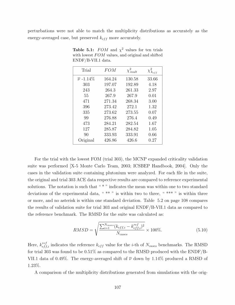
perturbations were not able to match the multiplicity distributions as accurately as the
energy-averaged case, but preserved keff more accurately.
Table 5.1: FOM and χ2 values for ten trialswith lowest FOM values, and original and shiftedENDF/B-VII.1 data.
Trial FOM χ2mult χ2
keff
ν -1.14% 164.24 130.58 33.66303 197.07 192.89 4.18243 264.3 261.33 2.9755 267.9 267.9 0.01471 271.34 268.34 3.00396 273.42 272.1 1.32335 273.62 273.55 0.0799 276.88 276.4 0.49473 284.21 282.54 1.67127 285.87 284.82 1.0590 333.93 333.91 0.66
Original 426.86 426.6 0.27
For the trial with the lowest FOM (trial 303), the MCNP expanded criticality validation
suite was performed [X-5 Monte Carlo Team, 2003; ICSBEP Handbook, 2004]. Only the
cases in the validation suite containing plutonium were analyzed. For each file in the suite,
the original and trial 303 ACE data respective results are compared to reference experimental
solutions. The notation is such that “ * ” indicates the mean was within one to two standard
deviations of the experimental data, “ ** ” is within two to three, “ *** ” is within three
or more, and no asterisk is within one standard deviation. Table 5.2 on page 108 compares
the results of validation suite for trial 303 and original ENDF/B-VII.1 data as compared to
the reference benchmark. The RMSD for the suite was calculated as:
RMSD =
√∑Ncases
i=1 (keff,i − krefeff,i)2
Ncases
× 100%. (5.10)
Here, krefeff,i indicates the reference keff value for the i-th of Ncases benchmarks. The RMSD
for trial 303 was found to be 0.51% as compared to the RMSD produced with the ENDF/B-
VII.1 data of 0.49%. The energy-averaged shift of ν down by 1.14% produced a RMSD of
1.23%.
A comparison of the multiplicity distributions generated from simulations with the orig-
107
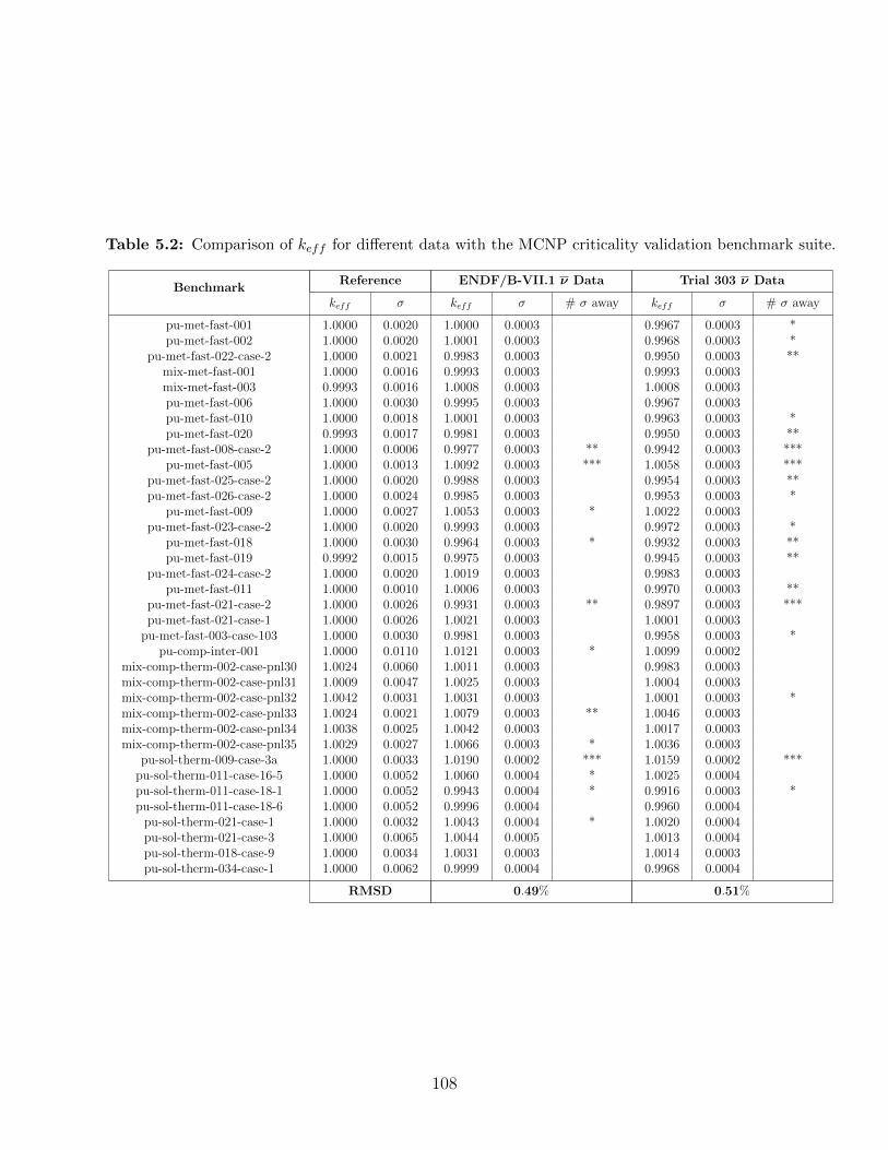
Table 5.2: Comparison of keff for different data with the MCNP criticality validation benchmark suite.
BenchmarkReference ENDF/B-VII.1 ν Data Trial 303 ν Data
keff σ keff σ # σ away keff σ # σ away
pu-met-fast-001 1.0000 0.0020 1.0000 0.0003 0.9967 0.0003 *pu-met-fast-002 1.0000 0.0020 1.0001 0.0003 0.9968 0.0003 *
pu-met-fast-022-case-2 1.0000 0.0021 0.9983 0.0003 0.9950 0.0003 **mix-met-fast-001 1.0000 0.0016 0.9993 0.0003 0.9993 0.0003mix-met-fast-003 0.9993 0.0016 1.0008 0.0003 1.0008 0.0003pu-met-fast-006 1.0000 0.0030 0.9995 0.0003 0.9967 0.0003pu-met-fast-010 1.0000 0.0018 1.0001 0.0003 0.9963 0.0003 *pu-met-fast-020 0.9993 0.0017 0.9981 0.0003 0.9950 0.0003 **
pu-met-fast-008-case-2 1.0000 0.0006 0.9977 0.0003 ** 0.9942 0.0003 ***pu-met-fast-005 1.0000 0.0013 1.0092 0.0003 *** 1.0058 0.0003 ***
pu-met-fast-025-case-2 1.0000 0.0020 0.9988 0.0003 0.9954 0.0003 **pu-met-fast-026-case-2 1.0000 0.0024 0.9985 0.0003 0.9953 0.0003 *
pu-met-fast-009 1.0000 0.0027 1.0053 0.0003 * 1.0022 0.0003pu-met-fast-023-case-2 1.0000 0.0020 0.9993 0.0003 0.9972 0.0003 *
pu-met-fast-018 1.0000 0.0030 0.9964 0.0003 * 0.9932 0.0003 **pu-met-fast-019 0.9992 0.0015 0.9975 0.0003 0.9945 0.0003 **
pu-met-fast-024-case-2 1.0000 0.0020 1.0019 0.0003 0.9983 0.0003pu-met-fast-011 1.0000 0.0010 1.0006 0.0003 0.9970 0.0003 **
pu-met-fast-021-case-2 1.0000 0.0026 0.9931 0.0003 ** 0.9897 0.0003 ***pu-met-fast-021-case-1 1.0000 0.0026 1.0021 0.0003 1.0001 0.0003
pu-met-fast-003-case-103 1.0000 0.0030 0.9981 0.0003 0.9958 0.0003 *pu-comp-inter-001 1.0000 0.0110 1.0121 0.0003 * 1.0099 0.0002
mix-comp-therm-002-case-pnl30 1.0024 0.0060 1.0011 0.0003 0.9983 0.0003mix-comp-therm-002-case-pnl31 1.0009 0.0047 1.0025 0.0003 1.0004 0.0003mix-comp-therm-002-case-pnl32 1.0042 0.0031 1.0031 0.0003 1.0001 0.0003 *mix-comp-therm-002-case-pnl33 1.0024 0.0021 1.0079 0.0003 ** 1.0046 0.0003mix-comp-therm-002-case-pnl34 1.0038 0.0025 1.0042 0.0003 1.0017 0.0003mix-comp-therm-002-case-pnl35 1.0029 0.0027 1.0066 0.0003 * 1.0036 0.0003
pu-sol-therm-009-case-3a 1.0000 0.0033 1.0190 0.0002 *** 1.0159 0.0002 ***pu-sol-therm-011-case-16-5 1.0000 0.0052 1.0060 0.0004 * 1.0025 0.0004pu-sol-therm-011-case-18-1 1.0000 0.0052 0.9943 0.0004 * 0.9916 0.0003 *pu-sol-therm-011-case-18-6 1.0000 0.0052 0.9996 0.0004 0.9960 0.0004
pu-sol-therm-021-case-1 1.0000 0.0032 1.0043 0.0004 * 1.0020 0.0004pu-sol-therm-021-case-3 1.0000 0.0065 1.0044 0.0005 1.0013 0.0004pu-sol-therm-018-case-9 1.0000 0.0034 1.0031 0.0003 1.0014 0.0003pu-sol-therm-034-case-1 1.0000 0.0062 0.9999 0.0004 0.9968 0.0004
RMSD 0.49% 0.51%
108
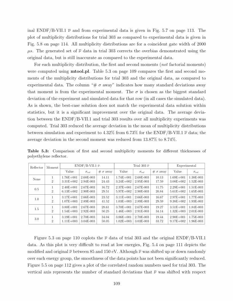
inal ENDF/B-VII.1 ν and from experimental data is given in Fig. 5.7 on page 113. The
plot of multiplicity distributions for trial 303 as compared to experimental data is given in
Fig. 5.8 on page 114. All multiplicity distributions are for a coincident gate width of 2000
µs. The generated set of ν data in trial 303 corrects the overbias demonstrated using the
original data, but is still inaccurate as compared to the experimental data.
For each multiplicity distribution, the first and second moments (not factorial moments)
were computed using mtool.pl. Table 5.3 on page 109 compares the first and second mo-
ments of the multiplicity distributions for trial 303 and the original data, as compared to
experimental data. The column “# σ away” indicates how many standard deviations away
that moment is from the experimental moment. The σ is chosen as the biggest standard
deviation of the experiment and simulated data for that row (in all cases the simulated data).
As is shown, the best-case solution does not match the experimental data solution within
statistics, but it is a significant improvement over the original data. The average devia-
tion between the ENDF/B-VII.1 and trial 303 results over all multiplicity experiments was
computed. Trial 303 reduced the average deviation in the mean of multiplicity distributions
between simulation and experiment to 4.32% from 6.73% for the ENDF/B-VII.1 ν data; the
average deviation in the second moment was reduced from 13.87% to 8.74%.
Table 5.3: Comparison of first and second multiplicity moments for different thicknesses ofpolyethylene reflector.
Reflector MomentENDF/B-VII.1 ν Trial 303 ν Experimental
Value σrel # σ away Value σrel # σ away Value σrel
None1 1.76E+001 2.68E-003 14.11 1.74E+001 2.68E-003 10.13 1.69E+001 1.38E-0032 3.31E+002 2.94E-003 24.43 3.24E+002 2.95E-003 17.59 3.08E+002 1.52E-003
0.51 2.40E+001 2.67E-003 16.72 2.37E+001 2.67E-003 11.75 2.29E+001 1.51E-0032 6.13E+002 2.90E-003 29.51 5.97E+002 2.90E-003 20.84 5.61E+002 1.65E-003
1.01 3.17E+001 2.66E-003 23.52 3.11E+001 2.66E-003 16.67 2.97E+001 1.77E-0032 1.07E+003 2.89E-003 41.52 1.03E+003 2.89E-003 29.59 9.38E+002 1.93E-003
1.51 3.80E+001 2.67E-003 28.61 3.70E+001 2.67E-003 19.27 3.51E+001 1.84E-0032 1.54E+003 2.92E-003 50.25 1.46E+003 2.91E-003 34.14 1.32E+003 2.01E-003
3.01 3.19E+001 2.70E-003 34.04 3.06E+001 2.70E-003 19.44 2.90E+001 1.75E-0032 1.11E+003 3.04E-003 58.05 1.02E+003 3.03E-003 33.72 9.17E+002 1.96E-003
Figure 5.3 on page 110 coplots the ν data of trial 303 and the original ENDF/B-VII.1
data. As this plot is very difficult to read at low energies, Fig. 5.4 on page 111 depicts the
modified and original ν between 85 and 150 eV. Although ν was shifted up or down randomly
over each energy group, the smoothness of the data points has not been significantly reduced.
Figure 5.5 on page 112 gives a plot of the correlated random numbers used for trial 303. The
vertical axis represents the number of standard deviations that ν was shifted with respect
109
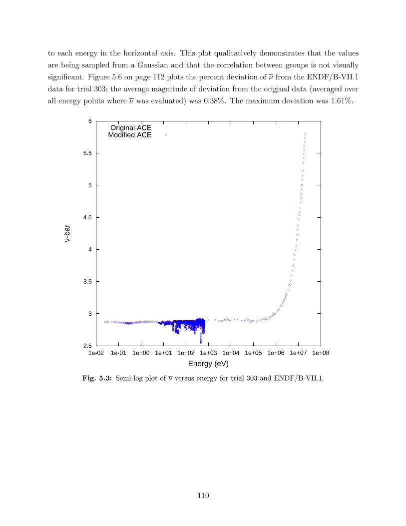
to each energy in the horizontal axis. This plot qualitatively demonstrates that the values
are being sampled from a Gaussian and that the correlation between groups is not visually
significant. Figure 5.6 on page 112 plots the percent deviation of ν from the ENDF/B-VII.1
data for trial 303; the average magnitude of deviation from the original data (averaged over
all energy points where ν was evaluated) was 0.38%. The maximum deviation was 1.61%.
2.5
3
3.5
4
4.5
5
5.5
6
1e-02 1e-01 1e+00 1e+01 1e+02 1e+03 1e+04 1e+05 1e+06 1e+07 1e+08
ν-bar
Energy (eV)
Original ACEModified ACE
Fig. 5.3: Semi-log plot of ν versus energy for trial 303 and ENDF/B-VII.1.
110
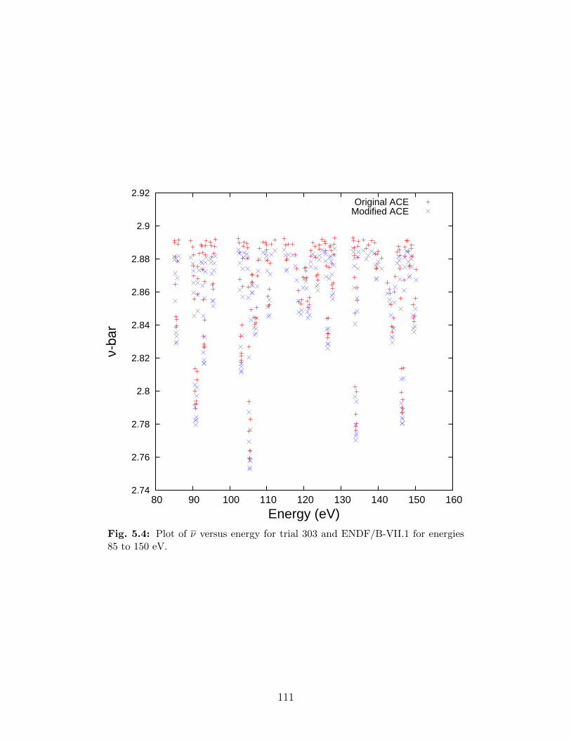
2.74
2.76
2.78
2.8
2.82
2.84
2.86
2.88
2.9
2.92
80 90 100 110 120 130 140 150 160
ν-b
ar
Energy (eV)
Original ACEModified ACE
Fig. 5.4: Plot of ν versus energy for trial 303 and ENDF/B-VII.1 for energies85 to 150 eV.
111
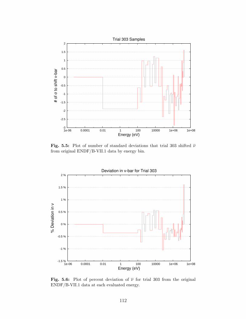
-3
-2.5
-2
-1.5
-1
-0.5
0
0.5
1
1.5
2
1e-06 0.0001 0.01 1 100 10000 1e+06 1e+08
# o
f σ
to s
hift
ν-bar
Energy (eV)
Trial 303 Samples
Fig. 5.5: Plot of number of standard deviations that trial 303 shifted νfrom original ENDF/B-VII.1 data by energy bin.
-1.5 %
-1 %
-0.5 %
0 %
0.5 %
1 %
1.5 %
2 %
1e-06 0.0001 0.01 1 100 10000 1e+06 1e+08
% D
evia
tio
n in
ν
Energy (eV)
Deviation in ν-bar for Trial 303
Fig. 5.6: Plot of percent deviation of ν for trial 303 from the originalENDF/B-VII.1 data at each evaluated energy.
112
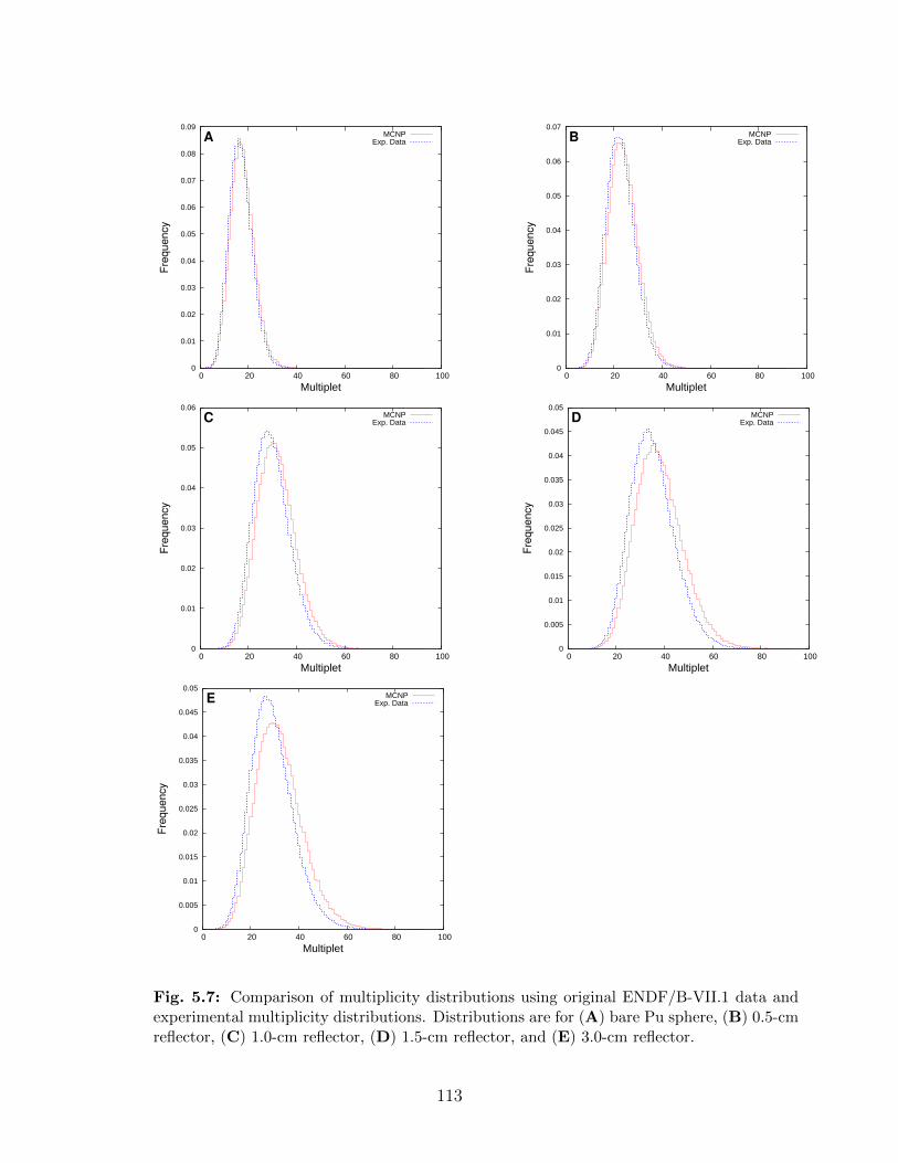
0
0.01
0.02
0.03
0.04
0.05
0.06
0.07
0.08
0.09
0 20 40 60 80 100
Fre
qu
en
cy
Multiplet
A MCNPExp. Data
0
0.01
0.02
0.03
0.04
0.05
0.06
0.07
0 20 40 60 80 100
Fre
qu
en
cy
Multiplet
B MCNPExp. Data
0
0.01
0.02
0.03
0.04
0.05
0.06
0 20 40 60 80 100
Fre
qu
en
cy
Multiplet
C MCNPExp. Data
0
0.005
0.01
0.015
0.02
0.025
0.03
0.035
0.04
0.045
0.05
0 20 40 60 80 100
Fre
qu
en
cy
Multiplet
D MCNPExp. Data
0
0.005
0.01
0.015
0.02
0.025
0.03
0.035
0.04
0.045
0.05
0 20 40 60 80 100
Fre
qu
en
cy
Multiplet
E MCNPExp. Data
Fig. 5.7: Comparison of multiplicity distributions using original ENDF/B-VII.1 data andexperimental multiplicity distributions. Distributions are for (A) bare Pu sphere, (B) 0.5-cmreflector, (C) 1.0-cm reflector, (D) 1.5-cm reflector, and (E) 3.0-cm reflector.
113
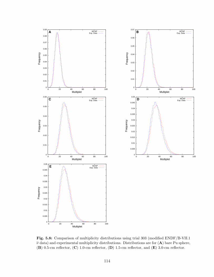
0
0.01
0.02
0.03
0.04
0.05
0.06
0.07
0.08
0.09
0 20 40 60 80 100
Fre
quency
Multiplet
A MCNPExp. Data
0
0.01
0.02
0.03
0.04
0.05
0.06
0.07
0 20 40 60 80 100
Fre
quency
Multiplet
B MCNPExp. Data
0
0.01
0.02
0.03
0.04
0.05
0.06
0 20 40 60 80 100
Fre
quency
Multiplet
C MCNPExp. Data
0
0.005
0.01
0.015
0.02
0.025
0.03
0.035
0.04
0.045
0.05
0 20 40 60 80 100
Fre
quency
Multiplet
D MCNPExp. Data
0
0.005
0.01
0.015
0.02
0.025
0.03
0.035
0.04
0.045
0.05
0 20 40 60 80 100
Fre
quency
Multiplet
E MCNPExp. Data
Fig. 5.8: Comparison of multiplicity distributions using trial 303 (modified ENDF/B-VII.1ν data) and experimental multiplicity distributions. Distributions are for (A) bare Pu sphere,(B) 0.5-cm reflector, (C) 1.0-cm reflector, (D) 1.5-cm reflector, and (E) 3.0-cm reflector.
114
5.7 Results of Cross Section Perturbations
The effect of the different cross section alteration schemes, discussed in Sections 5.4.3
and 5.4.4, are compared by the sum of the reduced chi-squared values for the multiplic-
ity distributions χ2mult given by Eq. (5.9). The first and second moments of multiplicity
distributions are compared to experimental results to determine when cross section alter-
ations produce high values of χ2mult because of over-correcting the original overbias in the
distributions. The average number of standard deviations that cross sections are shifted,
as calculated with Eq. (5.6), are given as a measure of how realistic the cross section alter-
ations are (where the variance data for that cross section were readily available); the sample
standard deviation of the number of standard deviations data was shifted is also given. The
chi-squared values for keff are also tabulated for comparison of the effect on the system to ν
alterations discussed in the previous section. Trials are labeled by the signed percent change
in a cross section of interest (α in Eq. (5.4)). For reference, a comparison of the multiplicity
distributions generated from simulations with the original ENDF/B-VII.1 cross sections and
from experimental data is given in Fig. 5.7 on page 113; the distributions for the “ν -1.14%”
trial are given in Fig. 5.10 on page 123.
5.7.1 Results of Capture Cross Section Perturbations
The results for case 1 of altering σc and σt discussed in Section 5.4.3 is given in Table 5.4 on
page 117. The plot of multiplicity distributions produced with 16% increased σc from case 1
and the five experimental distributions is given in Fig. 5.11 on page 124. Based on the values
of χ2mult in Table 5.4, increasing the value of σc decreases the discrepancy between the MCNP
and experimental multiplicity distributions. Significant alterations to the capture (and thus
total) cross section had to be made to create a noticeable improvement in χ2mult. As seen in
Table 5.4, the 16% increase in σc corresponds to a 3.5 and 6.9 standard deviation increase
in σf and σt , respectively. This set of data is well outside of statistical confidence, and the
correction to the multiplicity distributions is still not as good as that of the ν case. For
comparison, in the “-1.14% ν ” trial the value of ν was decreased 3.9 standard deviations,
on average, with s(#s(ν)) = 1.82 standard deviations. For most values of α, keff is not
effected in any statistically significant manner.
As demonstrated in Fig. 5.11, a 16% increase in σc with compensation in σt corrects the
overbias in multiplicity data produced by the original ENDF/B-VII.1 239Pu data, but in
most cases is still inaccurate as compared to the experimental data. The 3.0-cm scenario is
accurate to a high degree of precision. This indicates that χ2mult improvements are dominated
by corrections in the 3.0 cm scenario and energy-dependent alterations to σc may be able
115
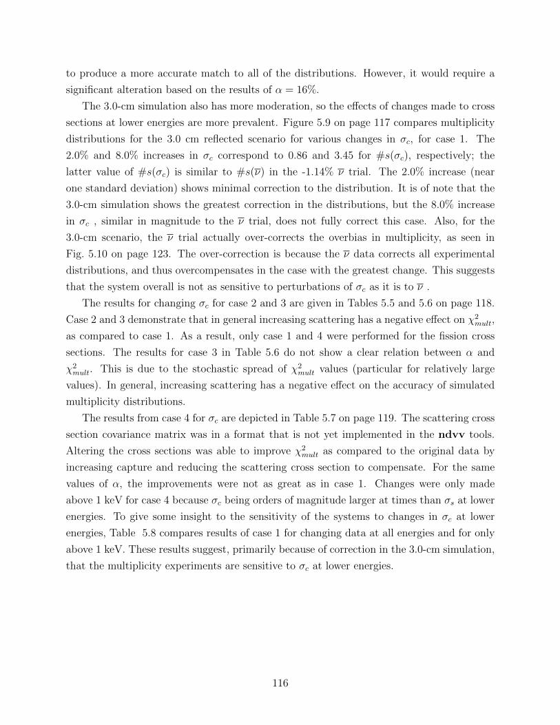
to produce a more accurate match to all of the distributions. However, it would require a
significant alteration based on the results of α = 16%.
The 3.0-cm simulation also has more moderation, so the effects of changes made to cross
sections at lower energies are more prevalent. Figure 5.9 on page 117 compares multiplicity
distributions for the 3.0 cm reflected scenario for various changes in σc, for case 1. The
2.0% and 8.0% increases in σc correspond to 0.86 and 3.45 for #s(σc), respectively; the
latter value of #s(σc) is similar to #s(ν) in the -1.14% ν trial. The 2.0% increase (near
one standard deviation) shows minimal correction to the distribution. It is of note that the
3.0-cm simulation shows the greatest correction in the distributions, but the 8.0% increase
in σc , similar in magnitude to the ν trial, does not fully correct this case. Also, for the
3.0-cm scenario, the ν trial actually over-corrects the overbias in multiplicity, as seen in
Fig. 5.10 on page 123. The over-correction is because the ν data corrects all experimental
distributions, and thus overcompensates in the case with the greatest change. This suggests
that the system overall is not as sensitive to perturbations of σc as it is to ν .
The results for changing σc for case 2 and 3 are given in Tables 5.5 and 5.6 on page 118.
Case 2 and 3 demonstrate that in general increasing scattering has a negative effect on χ2mult,
as compared to case 1. As a result, only case 1 and 4 were performed for the fission cross
sections. The results for case 3 in Table 5.6 do not show a clear relation between α and
χ2mult. This is due to the stochastic spread of χ2
mult values (particular for relatively large
values). In general, increasing scattering has a negative effect on the accuracy of simulated
multiplicity distributions.
The results from case 4 for σc are depicted in Table 5.7 on page 119. The scattering cross
section covariance matrix was in a format that is not yet implemented in the ndvv tools.
Altering the cross sections was able to improve χ2mult as compared to the original data by
increasing capture and reducing the scattering cross section to compensate. For the same
values of α, the improvements were not as great as in case 1. Changes were only made
above 1 keV for case 4 because σc being orders of magnitude larger at times than σs at lower
energies. To give some insight to the sensitivity of the systems to changes in σc at lower
energies, Table 5.8 compares results of case 1 for changing data at all energies and for only
above 1 keV. These results suggest, primarily because of correction in the 3.0-cm simulation,
that the multiplicity experiments are sensitive to σc at lower energies.
116
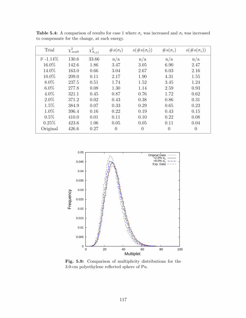
Table 5.4: A comparison of results for case 1 where σc was increased and σt was increasedto compensate for the change, at each energy.
Trial χ2mult χ2
keff#s(σt) s(#s(σt)) #s(σc) s(#s(σc))
ν -1.14% 130.6 33.66 n/a n/a n/a n/a16.0% 142.6 1.86 3.47 3.05 6.90 2.4714.0% 163.0 0.66 3.04 2.67 6.03 2.1610.0% 209.0 0.11 2.17 1.90 4.31 1.558.0% 237.5 0.51 1.74 1.52 3.45 1.246.0% 277.8 0.08 1.30 1.14 2.59 0.934.0% 321.1 0.45 0.87 0.76 1.72 0.622.0% 371.2 0.02 0.43 0.38 0.86 0.311.5% 384.9 0.07 0.33 0.29 0.65 0.231.0% 396.4 0.16 0.22 0.19 0.43 0.150.5% 410.0 0.01 0.11 0.10 0.22 0.080.25% 423.6 1.06 0.05 0.05 0.11 0.04
Original 426.6 0.27 0 0 0 0
0
0.005
0.01
0.015
0.02
0.025
0.03
0.035
0.04
0.045
0.05
0 20 40 60 80 100
Fre
qu
en
cy
Multiplet
Original Data+2.0% σc+8.0% σcExp. Data
Fig. 5.9: Comparison of multiplicity distributions for the3.0-cm polyethylene reflected sphere of Pu.
117
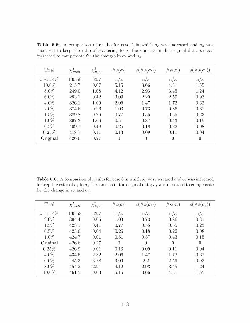
Table 5.5: A comparison of results for case 2 in which σc was increased and σs wasincreased to keep the ratio of scattering to σt the same as in the original data; σt wasincreased to compensate for the changes in σc and σs.
Trial χ2mult χ2
keff#s(σt) s(#s(σt)) #s(σc) s(#s(σc))
ν -1.14% 130.58 33.7 n/a n/a n/a n/a10.0% 215.7 0.07 5.15 3.66 4.31 1.558.0% 249.0 1.08 4.12 2.93 3.45 1.246.0% 283.1 0.42 3.09 2.20 2.59 0.934.0% 326.1 1.09 2.06 1.47 1.72 0.622.0% 374.6 0.26 1.03 0.73 0.86 0.311.5% 389.8 0.26 0.77 0.55 0.65 0.231.0% 397.3 1.66 0.51 0.37 0.43 0.150.5% 409.7 0.48 0.26 0.18 0.22 0.080.25% 418.7 0.11 0.13 0.09 0.11 0.04
Original 426.6 0.27 0 0 0 0
Table 5.6: A comparison of results for case 3 in which σc was increased and σs was increasedto keep the ratio of σc to σs the same as in the original data; σt was increased to compensatefor the change in σc and σs.
Trial χ2mult χ2
keff#s(σt) s(#s(σt)) #s(σc) s(#s(σc))
ν -1.14% 130.58 33.7 n/a n/a n/a n/a2.0% 394.4 0.05 1.03 0.73 0.86 0.311.5% 423.1 0.41 0.77 0.55 0.65 0.230.5% 423.6 0.04 0.26 0.18 0.22 0.081.0% 424.7 0.01 0.51 0.37 0.43 0.15
Original 426.6 0.27 0 0 0 00.25% 426.9 0.01 0.13 0.09 0.11 0.044.0% 434.5 2.32 2.06 1.47 1.72 0.626.0% 445.3 3.28 3.09 2.2 2.59 0.938.0% 454.2 2.91 4.12 2.93 3.45 1.2410.0% 461.5 9.03 5.15 3.66 4.31 1.55
118
Table 5.7: A comparison of results for case 4 in which σc wasincreased and σs was decreased to keep σt the same as in theoriginal data, for neutron energies greater than 1 keV.
Trial χ2mult χ2
keff#s(σc) s(#s(σc))
ν -1.14% 130.58 33.7 n/a n/a10.0% 345.1 0.22 4.04 1.218.0% 359.9 0.04 3.23 0.966.0% 372.7 1.11 2.42 0.724.0% 390.9 0.01 1.62 0.482.0% 408.8 0.13 0.81 0.241.5% 410.9 0.02 0.61 0.181.0% 417.9 0.01 0.40 0.120.5% 422.1 0.18 0.20 0.060.25% 425.4 0.04 0.10 0.03
Original 426.6 0.27 0 0
Table 5.8: A comparison of results for case 1 in which σc was increased and σs was decreasedto keep σt the same. Changes were made to cross sections for neutron energies above Ecut.
αχ2mult #s(σc) s(#s(σc))
Ecut = 1 keV Ecut = 0 Ecut = 1 keV Ecut = 0 Ecut = 1 keV Ecut = 0
10.0% 349.9 209.03 4.04 4.31 1.21 1.554.0% 395.35 321.1 1.62 1.72 0.48 0.622.0% 410.0 371.15 0.81 0.86 0.24 0.311.0% 420.7 396.4 0.40 0.43 0.12 0.150.5% 421.2 410.02 0.20 0.22 0.06 0.080.25% 423.5 423.59 0.10 0.11 0.03 0.04
119
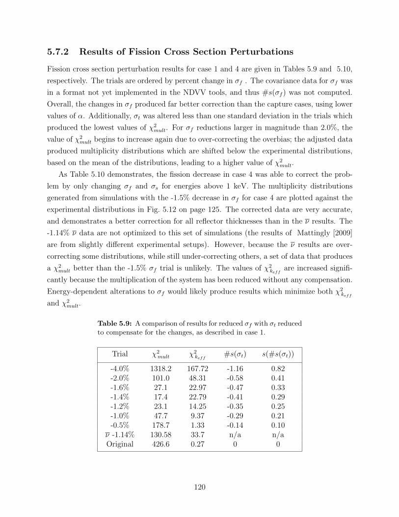
5.7.2 Results of Fission Cross Section Perturbations
Fission cross section perturbation results for case 1 and 4 are given in Tables 5.9 and 5.10,
respectively. The trials are ordered by percent change in σf . The covariance data for σf was
in a format not yet implemented in the NDVV tools, and thus #s(σf ) was not computed.
Overall, the changes in σf produced far better correction than the capture cases, using lower
values of α. Additionally, σt was altered less than one standard deviation in the trials which
produced the lowest values of χ2mult. For σf reductions larger in magnitude than 2.0%, the
value of χ2mult begins to increase again due to over-correcting the overbias; the adjusted data
produced multiplicity distributions which are shifted below the experimental distributions,
based on the mean of the distributions, leading to a higher value of χ2mult.
As Table 5.10 demonstrates, the fission decrease in case 4 was able to correct the prob-
lem by only changing σf and σs for energies above 1 keV. The multiplicity distributions
generated from simulations with the -1.5% decrease in σf for case 4 are plotted against the
experimental distributions in Fig. 5.12 on page 125. The corrected data are very accurate,
and demonstrates a better correction for all reflector thicknesses than in the ν results. The
-1.14% ν data are not optimized to this set of simulations (the results of Mattingly [2009]
are from slightly different experimental setups). However, because the ν results are over-
correcting some distributions, while still under-correcting others, a set of data that produces
a χ2mult better than the -1.5% σf trial is unlikely. The values of χ2
keffare increased signifi-
cantly because the multiplication of the system has been reduced without any compensation.
Energy-dependent alterations to σf would likely produce results which minimize both χ2keff
and χ2mult.
Table 5.9: A comparison of results for reduced σf with σt reducedto compensate for the changes, as described in case 1.
Trial χ2mult χ2
keff#s(σt) s(#s(σt))
-4.0% 1318.2 167.72 -1.16 0.82-2.0% 101.0 48.31 -0.58 0.41-1.6% 27.1 22.97 -0.47 0.33-1.4% 17.4 22.79 -0.41 0.29-1.2% 23.1 14.25 -0.35 0.25-1.0% 47.7 9.37 -0.29 0.21-0.5% 178.7 1.33 -0.14 0.10
ν -1.14% 130.58 33.7 n/a n/aOriginal 426.6 0.27 0 0
120
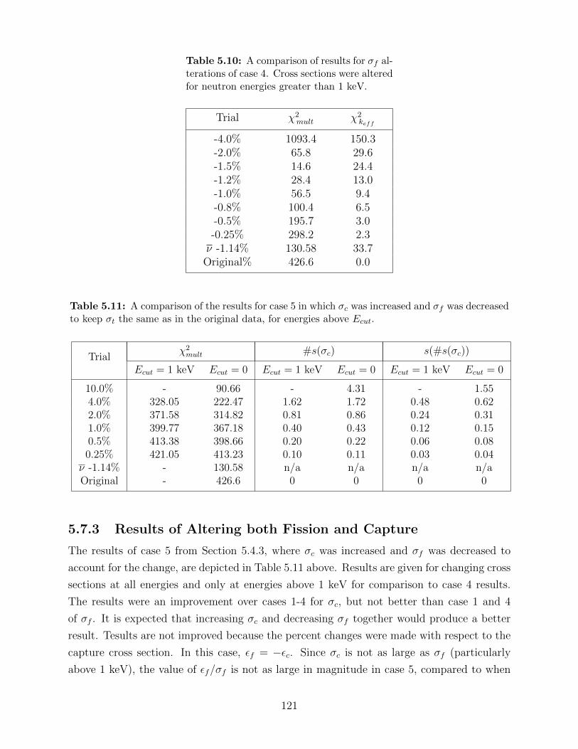
Table 5.10: A comparison of results for σf al-terations of case 4. Cross sections were alteredfor neutron energies greater than 1 keV.
Trial χ2mult χ2
keff
-4.0% 1093.4 150.3-2.0% 65.8 29.6-1.5% 14.6 24.4-1.2% 28.4 13.0-1.0% 56.5 9.4-0.8% 100.4 6.5-0.5% 195.7 3.0-0.25% 298.2 2.3ν -1.14% 130.58 33.7Original% 426.6 0.0
Table 5.11: A comparison of the results for case 5 in which σc was increased and σf was decreasedto keep σt the same as in the original data, for energies above Ecut.
Trialχ2mult #s(σc) s(#s(σc))
Ecut = 1 keV Ecut = 0 Ecut = 1 keV Ecut = 0 Ecut = 1 keV Ecut = 0
10.0% - 90.66 - 4.31 - 1.554.0% 328.05 222.47 1.62 1.72 0.48 0.622.0% 371.58 314.82 0.81 0.86 0.24 0.311.0% 399.77 367.18 0.40 0.43 0.12 0.150.5% 413.38 398.66 0.20 0.22 0.06 0.080.25% 421.05 413.23 0.10 0.11 0.03 0.04ν -1.14% - 130.58 n/a n/a n/a n/aOriginal - 426.6 0 0 0 0
5.7.3 Results of Altering both Fission and Capture
The results of case 5 from Section 5.4.3, where σc was increased and σf was decreased to
account for the change, are depicted in Table 5.11 above. Results are given for changing cross
sections at all energies and only at energies above 1 keV for comparison to case 4 results.
The results were an improvement over cases 1-4 for σc, but not better than case 1 and 4
of σf . It is expected that increasing σc and decreasing σf together would produce a better
result. Tesults are not improved because the percent changes were made with respect to the
capture cross section. In this case, εf = −εc. Since σc is not as large as σf (particularly
above 1 keV), the value of εf/σf is not as large in magnitude in case 5, compared to when
121

σf is altered directly. This result indicates that compensating for a change in σf with σc is
not effective relative to the statistical uncertainty in σc ; compensating for σf in σt or σs
produces a better result.
122
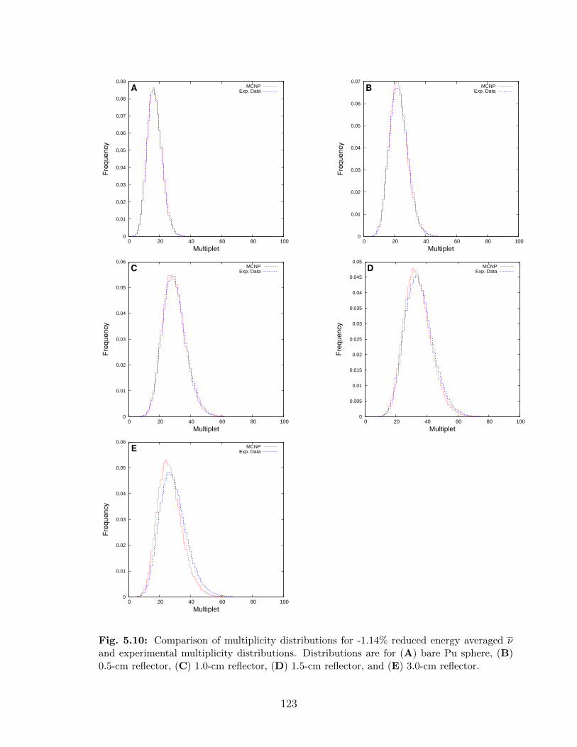
0
0.01
0.02
0.03
0.04
0.05
0.06
0.07
0.08
0.09
0 20 40 60 80 100
Fre
qu
en
cy
Multiplet
A MCNPExp. Data
0
0.01
0.02
0.03
0.04
0.05
0.06
0.07
0 20 40 60 80 100
Fre
qu
en
cy
Multiplet
B MCNPExp. Data
0
0.01
0.02
0.03
0.04
0.05
0.06
0 20 40 60 80 100
Fre
qu
en
cy
Multiplet
C MCNPExp. Data
0
0.005
0.01
0.015
0.02
0.025
0.03
0.035
0.04
0.045
0.05
0 20 40 60 80 100
Fre
qu
en
cy
Multiplet
D MCNPExp. Data
0
0.01
0.02
0.03
0.04
0.05
0.06
0 20 40 60 80 100
Fre
qu
en
cy
Multiplet
E MCNPExp. Data
Fig. 5.10: Comparison of multiplicity distributions for -1.14% reduced energy averaged νand experimental multiplicity distributions. Distributions are for (A) bare Pu sphere, (B)0.5-cm reflector, (C) 1.0-cm reflector, (D) 1.5-cm reflector, and (E) 3.0-cm reflector.
123
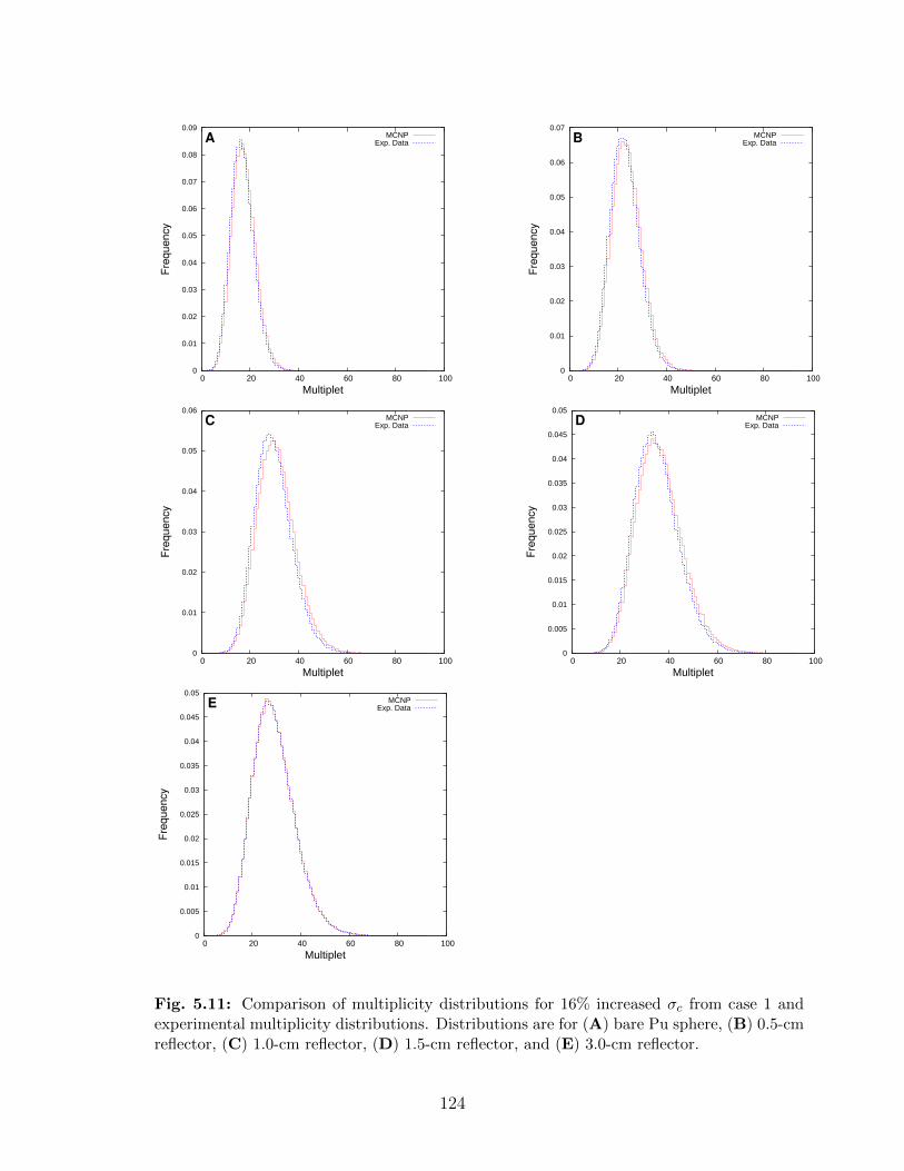
0
0.01
0.02
0.03
0.04
0.05
0.06
0.07
0.08
0.09
0 20 40 60 80 100
Fre
qu
en
cy
Multiplet
A MCNPExp. Data
0
0.01
0.02
0.03
0.04
0.05
0.06
0.07
0 20 40 60 80 100
Fre
qu
en
cy
Multiplet
B MCNPExp. Data
0
0.01
0.02
0.03
0.04
0.05
0.06
0 20 40 60 80 100
Fre
qu
en
cy
Multiplet
C MCNPExp. Data
0
0.005
0.01
0.015
0.02
0.025
0.03
0.035
0.04
0.045
0.05
0 20 40 60 80 100
Fre
qu
en
cy
Multiplet
D MCNPExp. Data
0
0.005
0.01
0.015
0.02
0.025
0.03
0.035
0.04
0.045
0.05
0 20 40 60 80 100
Fre
qu
en
cy
Multiplet
E MCNPExp. Data
Fig. 5.11: Comparison of multiplicity distributions for 16% increased σc from case 1 andexperimental multiplicity distributions. Distributions are for (A) bare Pu sphere, (B) 0.5-cmreflector, (C) 1.0-cm reflector, (D) 1.5-cm reflector, and (E) 3.0-cm reflector.
124
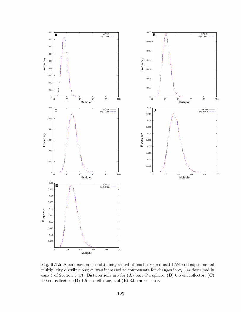
0
0.01
0.02
0.03
0.04
0.05
0.06
0.07
0.08
0.09
0 20 40 60 80 100
Fre
qu
en
cy
Multiplet
A MCNPExp. Data
0
0.01
0.02
0.03
0.04
0.05
0.06
0.07
0 20 40 60 80 100
Fre
qu
en
cy
Multiplet
B MCNPExp. Data
0
0.01
0.02
0.03
0.04
0.05
0.06
0 20 40 60 80 100
Fre
qu
en
cy
Multiplet
C MCNPExp. Data
0
0.005
0.01
0.015
0.02
0.025
0.03
0.035
0.04
0.045
0.05
0 20 40 60 80 100
Fre
qu
en
cy
Multiplet
D MCNPExp. Data
0
0.005
0.01
0.015
0.02
0.025
0.03
0.035
0.04
0.045
0.05
0 20 40 60 80 100
Fre
qu
en
cy
Multiplet
E MCNPExp. Data
Fig. 5.12: A comparison of multiplicity distributions for σf reduced 1.5% and experimentalmultiplicity distributions; σs was increased to compensate for changes in σf , as described incase 4 of Section 5.4.3. Distributions are for (A) bare Pu sphere, (B) 0.5-cm reflector, (C)1.0-cm reflector, (D) 1.5-cm reflector, and (E) 3.0-cm reflector.
125
5.8 Conclusions
The work presented in this chapter demonstrates that by exclusively changing ν in an energy-
dependent manner, multiplicity distributions can be recreated more accurately than with
the original ENDF/B-VII.1 data, without changing criticality results significantly. Although
energy-dependent perturbations were not as effective as shifting the entire spectrum of ν,
the perturbations preserved keff and the statistical uncertainties. More trials would likely
produce an energy-dependent modified set of data that would preserve keff while matching
multiplicity distributions at least as accurately as an energy-averaged shift. The results
also demonstrate that when ν is calibrated during creation of nuclear data these multiplicity
experiments should be considered. Although the accuracy of criticality problems was reduced
somewhat for the new data, this is not entirely unexpected. If, on average, ν has been shifted
down to ensure multiplicity distributions match, it is likely some other area in the nuclear
data needs adjustment to compensate.
Upon review of the cross section results, increasing the value of σc generally decreases
the discrepancy between the MCNP and experimental multiplicity distributions. However,
the multiplicity results are not sensitive to σc relative to the uncertainties in σc and σt. De-
creasing σf was able to produce multiplicity distributions which match experimental results
very well, particularly by increasing σs to compensate. This is to be expected because ν
alterations improved multiplicity results. If relatively small decreases in the mean number of
fission neutrons released per fission improve results, then minor decreases in the probability
of fission occurring should also be effective. The covariance data would be needed to ensure
the alterations to σf were not statistically unreasonable. However, based on the best-case
results from changing σt and σf , increasing σt by less than one standard deviation, it is
likely that the σf perturbations are small relative to the statistical uncertainties in σf (σf is
a significant portion of σt, particularly for energies above 1 keV).
The results of case 2 and 3 for σc suggest that increasing σs has a negative effect on
multiplicity distributions, although case 4 decreased σf and was able to match multiplicity
distributions very well by increasing σs. In case 4 for σc , σs is decreased, but the results were
not able to produce a better improvement over changes in σt and σc. It is of note that when
a cross section of interest is increased and σt is adjusted to compensate, the probability of all
other events occurring is inherently decreased. Appendix A provides some insight into this
phenomena. These results suggest that the effectiveness of case 1 for σc is partially because
of the fact that the probability of fission occurring has been decreased. It is noted that the
χ2keff
value was not statistically increased in the majority of the σc alterations, unlike in the
σf cases, even at the large value of 16%.
126

5.9 Summary and Suggestions for Future Work
Future work should include more correlated sampling trials of ν data for 239Pu. Energy-
dependent sampling of σf , compensating with σs, should also be pursued in future work,
as it has the potential to provide the best correction to multiplicity distributions, while
preserving keff . For futures samples, more criticality test cases should be included to
introduce more energy-dependent restrictions on the data. For sampling of σf , a global
optimization scheme may need to be applied. Cross sections have many covariance energy
groups (400 for σt of 239Pu), as compared to the 50 groups of ν, and will require far more
trials and constraining problems if the purely random sampling approach is used. A global
optimization approach should be used that takes random walks through the phase space
(preventing the method from finding local minima) but is biased to pick results that produce
better solutions. Additionally, the global optimization scheme should generate data that is
statistically realistic, based on the covariance data.
In the ideal case, both ν and sets of cross sections would be simultaneously sampled
from covariance data. The ideal set of nuclear data would then be determined based on
simulation results. This approach is inherently limited by the large degrees of freedom
and heavy computational cost. The beginning of the necessary methods and programs
to perturb energy-dependent nuclear data to match multiplicity distributions have been
developed and tested. Additionally, by adjusting the Figure of Merit parameters, a better
match to criticality problems as desired by the user can be found. Results have demonstrated
that these simulations should be considered in validation and calibration of nuclear data,
particularly ν. Initial findings are encouraging that this method will provide a tool for
validating nuclear data, and generating data sets purposed for simulating specific problems
in nuclear engineering
127

Bibliography
Baum, E. M., Knox, H. D. and Miller, T. R. [2002], Nuclides and Isotopes: Chart of the
Nuclides, 16th edn.
Bellinger, S., Fronk, R., McNeil, W., Sobering, T. and McGregor, D. [2010], High Efficiency
Dual-Integrated Stacked Microstructured Solid-State Neutron Detectors, in “IEEE NSS
Conf”, Knoxville, TN, pp. 2008–2012.
Biju, K., Tripathy, S., Sunil, C. and Sarkar, P. [2012], “FLUKA Simulations of a Mod-
erated Reduced Weight High Energy Neutron Detection System”, Nuclear Instruments
and Methods in Physics Research Section A: Accelerators, Spectrometers, Detectors and
Associated Equipment 682(0), 54 – 58.
Brackenbush, L. W. [1983], “Spunit: A Computer Code for Multisphere Unfolding”.
Bramblett, R. [1960], “A New Type of Neutron Spectrometer”, Nuclear Instruments and
Methods 9(1), 1–12.
Brennan, J., Brubaker, E., Cooper, R., Gerling, M., Greenberg, C., Marleau, P., Mascaren-
has, N. and Mrowka, S. [2011], “Measurement of the Fast Neutron Energy Spectrum of
an 241Am-Be Source Using a Neutron Scatter Camera”, IEEE Transactions on Nuclear
Science 58(5), 2426 –2430.
Brooks, F. and Klein, H. [2002], “Neutron Spectrometry: a Historical Review and Present
Status”, Nuclear Instruments and Methods in Physics Research Section A: Accelerators,
Spectrometers, Detectors and Associated Equipment 476(1-2), 1 – 11. Int. Workshop on
Neutron Field Spectrometry in Science, Technology, and Radiation Protection.
Caruso, A. N., Oakes, T., Miller, W. et al. [2011], High Intrinsic Efficiency Solid State
Neutron Detector and Spectrometer, Presented at IEEE Nuclear Science Symposium: 3He
Replacement, Valencia, Spain.
128
Chadwick, M., Oblozinsky, P. et al. [2006], ENDF/B-VII.0: Next Generation Evaluated
Nuclear Data Library for Nuclear Science and Technology, in “Nuclear Data Sheets”,
107th edn, pp. 2931–3060.
Cooper, B., Bellinger, S., Caruso, A., Fronk, R., Miller, W., Oakes, T., Shultis, J., Sobering,
T. and McGregor, D. [2011], Neutron Energy Spectrum with Microstructured Semicon-
ductor Neutron Detectors, in “IEEE Nuclear Science Symposium”, Valencia, Spain.
Croft, S., Favalli, A., Hauck, D. K., Henzlova, D. and Santi, P. A. [2012], “Feynman Variance-
to-Mean in the Context of Passive Neutron Coincidence Counting”, Nuclear Instruments
and Methods in Physics Research Section A: Accelerators, Spectrometers, Detectors and
Associated Equipment 686(0), 136–144.
Dunn, P. F. [2005], Measurement and Data Analysis for Engineering and Science, McGraw
Hill, 1221 Avenue of the Americas, New York, NY 10020.
ENDF-6 Manual [2011], ENDF-6 Formats Manual, 2nd edn, Upton, NY.
Ensslin, N. [1998], “Application Guide to Neutron Multiplicity Counting”. Los Alamos
Report LA-13422-M.
Fayegh, R. K. [1993], “Neural Network Unfolding of Photon and Neutron Spectra Using an
NE-213 Scintillation Detector”, Nuclear Instruments Methods in Physics Research: Section
A, Accelerators, Spectrometers, Detectors and Associated Equipment 329(1-2), 269–276.
Feynman, R. P. [1946], “Statistical Behavior of Neutron Chains”. Los Alamos Report LA-
591-DEL.
Flaska, M. and Pozzi, S. [2007a], “Identification of Shielded Neutron Sources with the Liq-
uid Scintillator BC-501A Using a Digital Pulse Shape Discrimination Method”, Nuclear
Instruments and Methods in Physics Research Section A: Accelerators, Spectrometers, De-
tectors and Associated Equipment 577(3), 654 – 663.
Flaska, M. and Pozzi, S. [2007b], Pulse-Shape Discrimination got Identification of Neutron
Sources Using The BC-501A Liquid Scintillator, Oak ridge National Laboratory, Presented
at M&C + SNA, Monterey, California.
Grissom, J. T. and Koehler, D. R. [1971], “Data Smoothing”, American Journal of Physics
39(11), 1314–1320.
Hogg, R. V., McKean, J. W. and Craig, A. T. [2013], Introduction to Mathematical Statistics,
7th edn, Pearson Education, Inc., 501 Boylston Street, Suite 900, Boston, MA 02116.
129
IAEA Report 403 [2001], “Compendium of Neutron Spectra and Detector Responses for Ra-
diation Protection Purposes: Supplement to Technical Reports Series no. 318”, Technical
Report Series no. 403.
ICRU [2001], “Determination of Operational Dose Equivalent Quantities for Neutrons”,
ICRU Report 66.
ICSBEP Handbook [2004], “International Handbook of Evaluated Criticality Safety Bench-
mark Experiments”, Nuclear Energy Agency, NEA/NSC/DOC(95)03/I.
ISO [2000], Reference Neutron Radiations – Part 2: Calibration Fundamentals of Radiation
Protection Devices Related to the Basic Quantities Characterizing the Radiation Field,
Technical Report ISO 8529-2, Geneva, Switzerland.
Kouzes, R., Siciliano, E., Ely, J., Keller, P. and McConn, R. [2007], Passive Neutron De-
tection at Borders, in “Nuclear Science Symposium Conference Record, 2007. NSS ’07.
IEEE”, Vol. 2, pp. 1115 –1119.
Mattingly, J. K. [2009], Polyethylene-Reflected Plutonium Metal Sphere: Subcritical Neu-
tron and Gamma Measurements, Revision 2, Technical Report SAND2009-5804, Sandia
National Laboratory.
McLean, T. D. and Justus, A. L. [2012], “EAGLE Neutron Rem-Meter Dose Meaurements
at the Trident Laser Facility”, (LAUR-12-26418).
Miller, E. C., Mattingly, J. K. et al. [2010], “Simulations of Neutron Multiplicity Measure-
ments with MCNP-PoliMi”, (SAND2010-6830).
Miller, S. C. [1993], AFITBUNKI: A Modified Iterative Code to Unfold Neutron Spectra from
Bonner Sphere Detector Data, Master’s thesis, Air Force Inst. of Tech. Write-Patterson.
Mukherjee, B. [2002], “A High-Resolution Neutron Spectra Unfolding Method Using the
Genetic Algorithm Technique”, Nuclear Instruments and Methods in Physics Research
Section A: Accelerators, Spectrometers, Detectors and Associated Equipment 476, 247 –
251. International Workshop on Neutron Field Spectrometry in Science, Technology and
Radiation Protection.
Olsher, R. [2004], “Prescila: A New, Lightweight Neutron Rem Meter”, Health physics
86(6), 603–12.
Olsher, R. H. [2000], “Wendi: An Improved Neutron Rem Meter”, Health physics 79(2), 170–
81.
130
Press, W. H., Teukolsky, S. A., Vetterling, W. T. and Flannery, B. P. [1992], Numerical
Recipes in C: The Art of Scientific Computing, 2nd edn.
Reilly, D., Ensslin, N., Jr., H. S. and Kreiner, S., eds [1991], Passive Nondestructive Assay
of Nuclear Materials, Los Alamos National Laboratory, P.O. Box 1663, MS E540, Los
Alamos, NM 87545.
Rousseuw, P. J. and Molenberghs, G. [1993], “Transformation of Non Positive Semidefinite
Correlation Matrices”, Communication in Statistics: Theory and Methods 22(4), 965–984.
Ryan, B. C. [1998], Analysis Methods for Bonner Sphere Spectrometry, Master’s thesis,
Kansas State University, Manhattan, KS.
Shultis, J. and Faw, R. [2004], “An MCNP Primer”, Dept. of Mechanical and Nuclear
Engineering, Kansas State University.
Shultis, J. K. and Dunn, W. L. [2011], Exploring Monte Carlo Methods, 1st edn, Elsevier
Science, San Diego, CA.
Shultis, J. K. and Faw, R. E. [2000], Radiation Shielding, American Nuclear Society, Inc.,
555 North Kensignton Ave., La Grange Park, IL 60526.
Shultis, J. K. and Faw, R. E. [2008], Fundamentals of Nuclear Science and Engineering,
Taylor & Francis Group, 6000 Broken Sound Parkway NW, Suit 300, Boca raton, FL
33487.
Shultis, J. and McGregor, D. [2009], Design and performance considerations of perforated
semiconductor thermal-neutron detectors.
Solomon, C. J. [2011], Polyethylene Reflected Pu Multiplication Inference Simulations, num-
ber LAUR-11-03933, Los Alamos National Laboratory, Presented at Nuclear Criticality
Safety Program Subcritical Measurement Workshop, Los Alamos National Laboratory.
Sood, A., Solomon, C. J. et al. [2011], Direct Calculation of Measured Observables in a Mul-
tiplying Sub-Critical System, number LAUR-11-02434, Los Alamos National Laboratory,
Presented at INC, Edinburg, Scottland.
Stacey, W. [2007], Nuclear Reactor Physics, John Wiley & Sons.
Sweezy, J., Hertel, N. and Veinot, K. [2002], “BUMS: A Bonner Sphere Unfolding Made
Simple: An HTML Based Multisphere Neutron Spectrometer Unfolding Package”, Nuclear
Instruments and Methods in Physics Research Section A: Accelerators, Spectrometers,
131
Detectors and Associated Equipment 476, 263 – 269. International Workshop on Neutron
Field Spectrometry in Science, Technology and Radiation Protection.
Taylor, J. R. [1997], An Introduction to Error Analysis, 2nd edn, University Science Books,
Sausalito, California.
Thomas, D. and Alevra, A. [2002], “Bonner Sphere Spectrometers: A Critical Review”,
Nuclear Instruments and Methods in Physics Research Section A: Accelerators, Spectrom-
eters, Detectors and Associated Equipment 476(1–2), 12 – 20. Int. Workshop on Neutron
Field Spectrometry in Science, Technology and Radiation Protection.
Toraskar, J. and Melkonian, E. [1971], “Spontaneous Fission of 240Pu: Comparison with the
Slow-Neutron-Induced Fission of 239Pu”, Physical Review .
Toyokawa, H., Yohizawa, M., Uritani, A., Mori, C., Takeda, N. and Kudo, K. [1997], “Per-
formance of a Spherical Neutron Counter for Spectroscopy and Dosimetry”, IEEE Trans-
actions on Nuclear Science 44(3), 788 –791.
Tsoulfanidis, N. [1995], Measurement and Detection of Radiation, 2nd edn, Taylor & Francis,
Bristol, PA.
Twomey, S. [1963], “On the Numerical Solution of Fredholm Integral Equations of the First
Kind by the Inversion of the Linear System Produced by Quadrature”, J. ACM 10(1), 97–
101.
Vega-Carrillo, H., Ortiz-Rodriguez, J. and Martinez-Blanco, M. [2012], “NSDUAZ Unfolding
Package for Neutron Spectrometry and Dosimetry with Bonner Spheres”, Applied Radi-
ation and Isotopes 71, Supplement(0), 87 – 91. XII International Symposium on Solid
State Dosimetry.
X-5 Monte Carlo Team [2003], MCNP - A General N-Particle Transport Code, Version 5,
Volume I,II,II, Los Alamos National Laboratory. LA-UR-03-1987.
Yoshida, T., Tsujimura, N. and Yamano, T. [2011], “Development of a Hand-Held Fast
Neutron Survey Meter”, Radiation Protection Dosimetry 146(1-3), 72–75.
132
Appendix A
Changes in Probabilities ofInteraction Events
This section develops an intuitive explanation of the behavior caused by altering the total
interaction cross section, through a simplified example. Consider neutrons of a particular
energy traveling through a homogeneous system. Consider only two reactions: a reaction
of interest a and the occurrence of any other reaction, labeled as b. The total interaction
cross section is σt = σa + σb. The cross section σa is to be perturbed, and σt must be
adjusted to compensate. The probability of a neutron traveling a distance x to where it has
an interaction of type i is
P (Interaction i, x) = P (Interaction, x) ∗ P (Interaction i | Interaction, x)
= [1− e−σtx] σiσt,
(A.1)
where P (Interaction i | Interaction, x) denotes the conditional probability that an interactino
of type i occurs, given that an interaction at x has occured. This conditional probability,
given by σi/σt, is what was altered in in Section 5.7 by adjusting the cross sections. How-
ever, the marginal probability of interaction (the term in squared brackets) is also implicitly
adjusted. Consider the case in which σa is altered by εa, i.e., σ ′a = σa + εa. The total cross
section is then adjusted to compensate as σ ′t = σt + εa. For the value of P (Interaction a, x),
both the conditional and marginal probability in Eq. (A.1) have increased from the original
values to the perturbed values in a straightforward manner, so the probability of that inter-
action occurring has increased. Now, consider the change in probability for the unperturbed
reaction b. The probability of a neutron undergoing interaction b at x in the perturbed
system is given by
P ′(Interaction b) = p′b(x) =[1− e−σ ′
tx] σbσ ′t. (A.2)
In this case, since σ ′t is greater than σt, the probability of an interaction occuring has
133
increased, but the conditional probability of interaction b occurring has decreased. To de-
termine the net effect on pb(x) consider the Maclaurin series for exp (−σ ′tx):
p′b(x) =
[1− (1− σ ′tx+
(σ ′tx)2
2+O(σ ′3t x
3))
]σbσ ′t. (A.3)
Simplification yields
p′b(x) = σb x−σ ′tx
2
2−O(σ ′2t x
3)). (A.4)
In the original, unperturbed system, the probability of interaction b at x is given by
Eq. (A.4) with σt replacing σ ′t . The difference in pb(x) of the perturbed and original system
is
∆pb(x) = p′b(x)− pb(x) = −(σ ′t − σt)x2
2+O((σ ′2t − σ2
t )x3). (A.5)
Substituting for σ′t in the first term yields:
∆pb(x) = −εax2
2+O((σ ′2t − σ2
t )x3) (A.6)
The overall probability of interaction b occurring is ∝ −εa. Thus, altering a cross section
and adjusting the total cross section to compensate for the change inherently alters the
probablity of all other reactions occuring in the opposite direction.
134
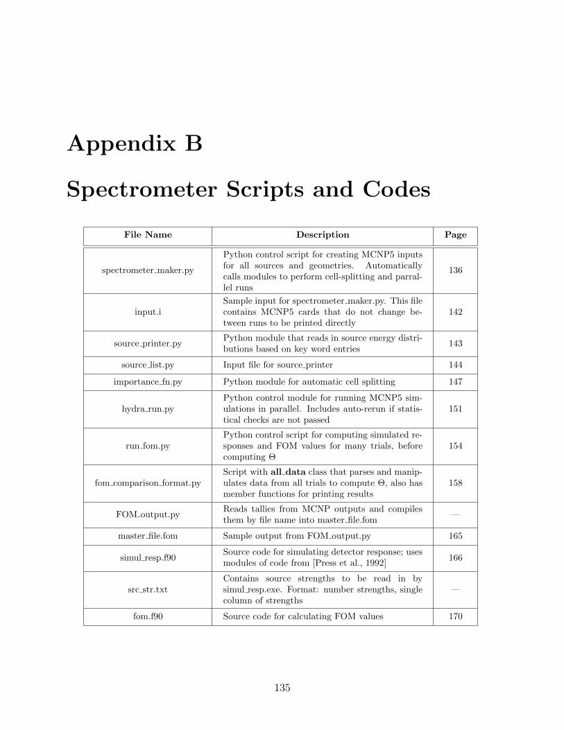
Appendix B
Spectrometer Scripts and Codes
File Name Description Page
spectrometer maker.py
Python control script for creating MCNP5 inputsfor all sources and geometries. Automaticallycalls modules to perform cell-splitting and parral-lel runs
136
input.iSample input for spectrometer maker.py. This filecontains MCNP5 cards that do not change be-tween runs to be printed directly
142
source printer.pyPython module that reads in source energy distri-butions based on key word entries
143
source list.py Input file for source printer 144
importance fn.py Python module for automatic cell splitting 147
hydra run.pyPython control module for running MCNP5 sim-ulations in parallel. Includes auto-rerun if statis-tical checks are not passed
151
run fom.pyPython control script for computing simulated re-sponses and FOM values for many trials, beforecomputing Θ
154
fom comparison format.pyScript with all data class that parses and manip-ulates data from all trials to compute Θ, also hasmember functions for printing results
158
FOM output.pyReads tallies from MCNP outputs and compilesthem by file name into master file.fom
—
master file.fom Sample output from FOM output.py 165
simul resp.f90Source code for simulating detector response; usesmodules of code from [Press et al., 1992]
166
src str.txtContains source strengths to be read in bysimul resp.exe. Format: number strengths, singlecolumn of strengths
—
fom.f90 Source code for calculating FOM values 170
135

spectrometer maker.py: Generate and Run MCNP5 Filesimport shutil # for copying files
import os # for directories and chmod etc.
import stat # for chmoding to user access
import subprocess # for running programs
import re # for regexps
import source_printer #reads sources from master file and prints them
import importance_fn #deternubes the "imp:n/p" in a file
import hydra_run #runs mcnp on hydra
# function for default file reading
def readinput(inputfilename):
input = open(inputfilename)
a = []
for line in input:
a.append(line)
input.close()
return a;
# directorymaker
def makedirectory(dir):
if not os.path.exists(dir):
os.makedirs(dir)
os.chmod(dir, stat.S_IRWXU)
else:
os.chmod(dir, stat.S_IRWXU)
# prints a list of stuff with some justification to a file
def printer(file, stuff, justified):
for item in stuff:
temp = str(item)
if(len(temp) < justified):
file.write(temp.ljust(justified))
else:
file.write(temp.ljust(len(temp)+2))
return
# prints stuff from the initial file
def initial_printer(ifile, initialfile, initialfile_counter):
count = 0;
for line in initialfile:
if (count < initialfile_counter):
count +=1
continue
else:
# prints from initialfile until it finds a "c *" line
temp = line.split()
if (len(temp) > 1):
if (temp[1] == ’*’):
break
ifile.write(line)
count+=1
return count+1
#moves file to a directory OVERWRITING any files in the way
def move_dir(file_name, dir):
os.chdir(dir)
if os.path.exists(file_name):
print "IM IN YOUR DIRECTORY DELETING YOUR FILES!"
os.remove(file_name)
os.chdir("..")
shutil.move(file_name, dir)
136
#makes a batch file for all mcnp files. A list of lists of names of files for each directory in directories.
def make_batch(mcnp_names, directories):
print "Enter in the name of the batch file (no extension)"
name = raw_input()
print "How many nodes (seperate files to run) do you want?"
number = raw_input()
batch = []
for t in range(int(number)): #open a file for each node
batch.append(open(name+str(t)+".bat", "w"))
#determine number of files to be printed per batch
files_per_batch = 0
for i in mcnp_names:
files_per_batch += len(i)
files_per_batch = int(files_per_batch/float(number))
filecount = 0 #keep track of how many files have been printed on each
t=0 #which batch file are you in
for direct in range(len(directories)): #loop through each directory
batch[t].write("cd %s\n" % directories[direct]) #change from the main directory to the current one
for name in mcnp_names[direct]: #writes
if (filecount == files_per_batch and t != (int(number)-1)): #extra file because of odd numbers
t+=1 #next file
batch[t].write("cd %s\n" %directories[direct])
filecount=0
tempstring = name.replace(".i",".o")
batch[t].write("mcnp5 i=%s o= %s\n" % (name, tempstring))
filecount+=1 #increment nout of how many files printed per batch
batch[t].write("erase runt*\n")
batch[t].write("cd ..\n")
for t in batch:
t.close()
#searchs a line for a string, returns true if found, else false
def search_for(line, string):
pattern = re.compile(str(string))
if (pattern.search(line)):
return True
else:
return False
# ***********main ****************
def main():
#output info
all_source_names = []
# constants throughout
mat_li = 2
mat_hdpe = 1
mat_board = 4
mat_cd = 3
source_erg_dist = 1
#densities
dens_li = -0.0835
dens_hdpe = -0.9500
dens_board = 0.00053
dens_cd = -8.65
#input data
output_data = [] #output list to be printed
names = [] #output file names
137
directories = [] #name of detector types that directories are made to store all the different stuff
detector_start = 100.0
cyl_radius = [10.0, 9.5, 9.0, 8.0, 7.5, 7.0, 6.5, 6.0, 5.5, 5.0, 4.5, 4.0] #outer radius of HDPE
#must be bigger than the size of the detectors and the board
number_detectors =[6,6,6,6,6,6,6,7,7,7,7,7,7,7,8,8,8,8,8,8,8]
poly_thick = [4.0, 4.5, 5.0, 5.5, 6.0, 6.5, 7.0, \
3.5, 4.0, 4.5, 5.0, 5.5, 6.0, 6.5, \
3.0, 3.5, 4.0, 4.5, 5.0, 5.5, 6.0 ]
cyl_radius = [6.0]*len(poly_thick)
if (len(poly_thick) != len(number_detectors)):
print "your lengths don’t match"
exit()
cd_thick = 0.1
board_thick = 0.157
board_width = 1.1
li_thick = 0.1
normalization = 0.00333286*li_thick/0.1 # constant used for FMn tally card to account for efficiency
#cell numbers for the RPP that define the detector and the boards and CYL for boundary
det_box = 35
board_box = 40
outer_cyl = 30
source_list = readinput("source_names.txt")
for i in range(len(source_list)):
source_list[i] =source_list[i].strip(’\n’)
#check to see if this is on hydra or a pc. Use hydra_check for particle balance function and mcnp runs
hydra_check = hydra_run.hydra_machine()
if hydra_check:
num_nodes = raw_input("Enter the number of nodes: ")
for det in range(len(number_detectors)):
initialfile = readinput(’input.i’) #stuff to print throughout
directories.append("Det"+str(number_detectors[det])+"PE"+str(poly_thick[det])+"R"+str(cyl_radius[det]))
makedirectory(directories[det])
names = []
for source in source_list:
#open a file for each source
names.append(source+".i")
ifile = open(source+".i", "w")
initialfile_counter = 0 # keeps track of where you are in the prebuilt input file
initialfile_counter = initial_printer(ifile, initialfile, initialfile_counter) #returns
#where you are at in the file, after the "*" break, see function for more details
li_front = ([],[]) #[surface numbers], [locations in x plane], front is front of li cell
li_back = ([],[]) #back of li cell
cd_front = ([],[])
li_cells = []
poly_cells = []
poly_cells_annulus=[]
cd_cells = []
cd_back = ([], [])
board_cells = []
#Create surfaces of the detector, front surfaces 100’s, back 1100’s, cd front 200’s, cd back 1200’s
for i in range((number_detectors[det])):
#front of detectors
if (i==0):
li_front[1].append(detector_start) #create the initial surface
else:
li_front[1].append(li_front[1][-1]+poly_thick[det]) #start of the current detector
#other surfaces - each one is a thickness offset by the thickness of the last detector
li_back[1].append(li_front[1][-1]+li_thick)
cd_front[1].append(li_back[1][-1]+board_thick)
cd_back[1].append(cd_front[1][-1]+cd_thick)
138
#create surface numbers and cell numbers for all surfaces
# --- cd cells: 500, polycells around detectors 11, 21, etc, licells: 10, 20, 30.., board_cells: 600’s,
# poly behind cd: 400’s---
for i in range((number_detectors[det])):
li_front[0].append(100+i)
li_back[0].append(1100+i)
cd_front[0].append(200+i)
cd_back[0].append(1200+i)
cd_cells.append(500+i)
#label detectors in increments of 10
li_cells.append(10*(i+1))
poly_cells_annulus.append(10*(i+1)+1) #annulus of HDPE around the lithium and board
poly_cells.append(400+i)
board_cells.append(600+i)
#add one more li_cell that is equal to the back of the detector
li_front[0].append(li_front[0][-1]+1)
li_front[1].append(li_front[1][-1]+poly_thick[det])
#print the cell cards:
# **************************************************************************************
#DEBUG: DIfferent for if you want a poly sheet in back or not
poly_sheet = False
if(not poly_sheet):
print poly_cells.pop(-1) #DEBUG is there a poly sheet in back or not
li_front[1][-1] = li_front[1][-2]+cd_thick+board_thick+li_thick
#determine the array_width, the width of the RPP that holds all the poly
array_width = li_front[1][-1] - li_front[1][0]
#print the Li regions, board, and the poly around them
imp = 1.0
ifile.write("c ---- detector chunks, breadboards, and surounding poly annuli ----\n")
for cell in range(number_detectors[det]):
#print detector
printer(ifile, [li_cells[cell], mat_li, str(dens_li), " "], 4)
printer(ifile, [li_front[0][cell], -1*li_back[0][cell], -1*det_box], 6)
ifile.write(" imp:n=%6.2f $detector at %.0f cm \n" % (imp, li_front[1][cell]-100))
#print bread board
printer(ifile, [board_cells[cell], mat_board, str(dens_board), " "], 4)
printer(ifile, [li_back[0][cell], -1*cd_front[0][cell], -1*board_box], 6)
ifile.write(" imp:n=%6.2f $breadboard at %.0f cm \n" % (imp, li_front[1][cell]-100))
#print poly annuli outside of the lithium and breadboard
if (cell == 0):
printer(ifile, [poly_cells_annulus[cell], "0", " ", " "], 4)
printer(ifile, [li_front[0][cell], -1*cd_front[0][cell], -1*outer_cyl, "(("+str(det_box)+" "+
str(-1*li_back[0][cell])+"):"+str(board_box)+")"], 4)
ifile.write("imp:n=%6.2f $Voided annulus at %.0f cm \n" % (imp, li_front[1][cell]-100))
else:
printer(ifile, [poly_cells_annulus[cell], mat_hdpe, str(dens_hdpe)+"00", " "], 4)
printer(ifile, [li_front[0][cell], -1*cd_front[0][cell], -1*outer_cyl, "(("+str(det_box)+" "+
str(-1*li_back[0][cell])+"):"+str(board_box)+")"], 4)
ifile.write("imp:n=%6.2f $HDPE annulus at %.0f cm \n" % (imp, li_front[1][cell]-100))
#print the Cd behind the detectors
ifile.write("c ---- Cd slices behind detectors ----\n")
imp= 1.0
for cell in range(len(cd_cells)):
printer(ifile, [cd_cells[cell], mat_cd, str(dens_cd)+"00", " "], 4)
printer(ifile, [cd_front[0][cell], -1*cd_back[0][cell], -1*outer_cyl], 6)
139
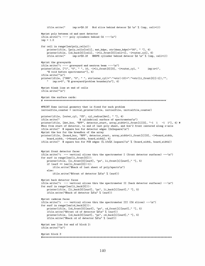
ifile.write(" imp:n=%6.2f $cd slice behind detecor %d \n" % (imp, cell+1))
#print poly between cd and next detector
ifile.write("c ---- poly cylinders behind Cd ----\n")
imp = 1.0
for cell in range(len(poly_cells)):
printer(ifile, [poly_cells[cell], mat_hdpe, str(dens_hdpe)+"00", " "], 4)
printer(ifile, [cd_back[0][cell], -1*li_front[0][cell+1], -1*outer_cyl], 6)
ifile.write(" imp:n=%6.2f $HDPE cylinder behind detecor %d \n" % (imp, cell+1))
#print the graveyards
ifile.write("c ---- graveyard and neutron beam ----\n")
printer(ifile, ["1", "0", " ", 10, -1*li_front[0][0], -1*outer_cyl, " imp:n=1",
"$ void before spectrometer"], 4)
ifile.write("\n")
printer(ifile, ["999", "0", " ", str(outer_cyl)+":"+str(-10)+":"+str(li_front[0][-1]),"",
" imp:n=0", "$ graveyard/problem boundary\n"], 4)
#print blank line at end of cells
ifile.write("\n")
#print the surface cards:
# **************************************************************************************
#PRINT Some initial geometry that is fixed for each problem
initialfile_counter = initial_printer(ifile, initialfile, initialfile_counter)
printer(ifile, [outer_cyl, "CX", cyl_radius[det], " "], 4)
ifile.write(" $ cylindrical surface of spectrometer\n")
printer(ifile, [det_box, "RPP", detector_start, array_width+li_front[1][0], "-1 1 -1 1"], 4) #
#box from start of detector, to end of last poly sheet, and 4cm^2 front centered along x-axis
ifile.write(" $ square box for detector edges (2x2square)\n")
#print the box for the breadbox of the array
printer(ifile, [board_box, "RPP", detector_start, array_width+li_front[1][0], -1*board_width,
board_width, -1*board_width, board_width], 4)
ifile.write(" $ square box for PCB edges (%.1fx%f.1square)\n" % (board_width, board_width))
#print front detector faces
ifile.write("c --- vertical slices thru the spectrometer I (front detector surfaces) ---\n")
for surf in range(len(li_front[0])):
printer(ifile, [li_front[0][surf], "px", li_front[1][surf]," "], 5)
if (surf == len(li_front[0])-1):
ifile.write("$back of last sheet of poly/spectr\n")
else:
ifile.write("$front of detector %d\n" % (surf))
#print back detector faces
ifile.write("c --- vertical slices thru the spectrometer II (back detector surfaces) ---\n")
for surf in range(len(li_back[0])):
printer(ifile, [li_back[0][surf], "px", li_back[1][surf]," "], 5)
ifile.write("$back of detector %d\n" % (surf))
#print cadmium faces
ifile.write("c --- vertical slices thru the spectrometer III (Cd slices) ---\n")
for surf in range(len(cd_back[0])):
printer(ifile, [cd_front[0][surf], "px", cd_front[1][surf]," "], 5)
ifile.write("$front cd of detector %d\n" % (surf))
printer(ifile, [cd_back[0][surf], "px", cd_back[1][surf]," "], 5)
ifile.write("$back cd of detector %d\n" % (surf))
#print new line for end of block 2:
ifile.write("\n")
#print block 3
#*******************************************************************************************
140
#print the source spatial definition
initialfile_counter = initial_printer(ifile, initialfile, initialfile_counter)
ifile.write("SI2 0 %.2f $ radial sampling range: 0 to Rmax\n" % float(cyl_radius[det]))
#print the source energy distribution:
source_data = source_printer.get_source("source_list.txt", source)
source_printer.print_source(ifile, source_data, source_erg_dist)
#print some physics settings
initialfile_counter = initial_printer(ifile, initialfile, initialfile_counter)
#print detector:
ifile.write("F4:N ")
for cell in li_cells:
ifile.write("%d " % cell) #print each of the detector cells
ifile.write("\nTF4 %d 7j\n" % len(li_cells)) #tells the tally fluctuation chart to optimize
#the last detector cell (the normalization cell), the 7j just means skip all the other
#entries, ncessary for the card used
#print the rest of the detector and the material cards
initialfile_counter = initial_printer(ifile, initialfile, initialfile_counter)
ifile.close()
# RUN PARTICLE BALANCE ON EACH FILE TO GET THE CORRECT IMPORTANCE FUNCTION FOR EACH:
# *******************************************************************************************
importance_fn.particle_balance(names[-1], cd_cells, [li_cells, poly_cells, poly_cells_annulus,
board_cells], 300000, ’n’, 1.00, hydra_check) #names[-1] is curent source file name, li_cells
#is the ones being balance, particle type is , hydra_check is whether or not this is a hydra run
#also case sensitive
#move the source files to the correct directory so you dont overwrite them
move_dir(source+".i", directories[det]) #store files
#append name
all_source_names.append(names)
#create an output list of all the directories
print directories
directories_file = open("directories.txt", "w")
for derp in directories:
directories_file.write(derp+"\n")
directories_file.close()
if (hydra_check == True):
count = 0
for i in directories:
for name in names:
count +=1
print "Running file: %s/%s, file %i of %i" % (i, name, count, len(directories)*len(names))
hydra_run.hydra_mcnp_run(name, i, "same", num_nodes, auto_rerun = True, tallies = ["4"])
#^^^i is directory of files, "same" for no output directory, auto rerun reruns if not
# enough particles, tallies is which to make sure converged
else: #Local run with batch files on 4 processors
break_check = True
make_batch(all_source_names, directories)
if __name__ == "__main__":
main()
141
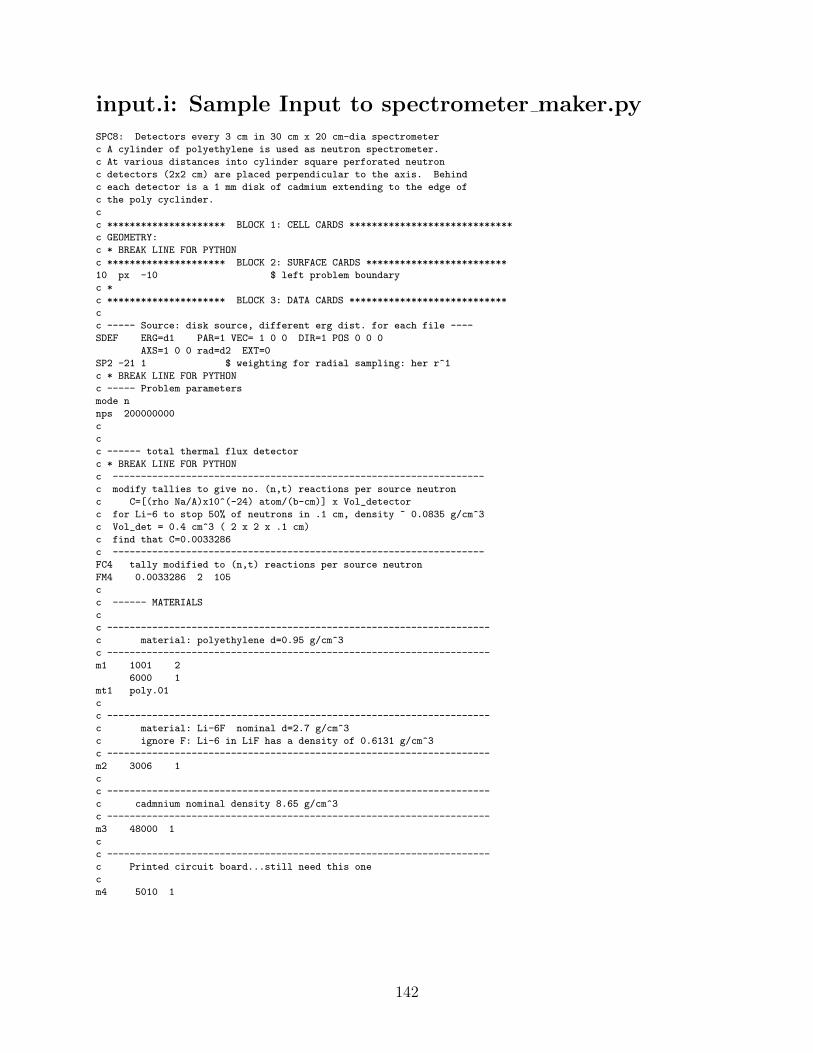
input.i: Sample Input to spectrometer maker.pySPC8: Detectors every 3 cm in 30 cm x 20 cm-dia spectrometer
c A cylinder of polyethylene is used as neutron spectrometer.
c At various distances into cylinder square perforated neutron
c detectors (2x2 cm) are placed perpendicular to the axis. Behind
c each detector is a 1 mm disk of cadmium extending to the edge of
c the poly cyclinder.
c
c ********************* BLOCK 1: CELL CARDS *****************************
c GEOMETRY:
c * BREAK LINE FOR PYTHON
c ********************* BLOCK 2: SURFACE CARDS *************************
10 px -10 $ left problem boundary
c *
c ********************* BLOCK 3: DATA CARDS ****************************
c
c ----- Source: disk source, different erg dist. for each file ----
SDEF ERG=d1 PAR=1 VEC= 1 0 0 DIR=1 POS 0 0 0
AXS=1 0 0 rad=d2 EXT=0
SP2 -21 1 $ weighting for radial sampling: her r^1
c * BREAK LINE FOR PYTHON
c ----- Problem parameters
mode n
nps 200000000
c
c
c ------ total thermal flux detector
c * BREAK LINE FOR PYTHON
c ------------------------------------------------------------------
c modify tallies to give no. (n,t) reactions per source neutron
c C=[(rho Na/A)x10^(-24) atom/(b-cm)] x Vol_detector
c for Li-6 to stop 50% of neutrons in .1 cm, density ~ 0.0835 g/cm^3
c Vol_det = 0.4 cm^3 ( 2 x 2 x .1 cm)
c find that C=0.0033286
c ------------------------------------------------------------------
FC4 tally modified to (n,t) reactions per source neutron
FM4 0.0033286 2 105
c
c ------ MATERIALS
c
c --------------------------------------------------------------------
c material: polyethylene d=0.95 g/cm^3
c --------------------------------------------------------------------
m1 1001 2
6000 1
mt1 poly.01
c
c --------------------------------------------------------------------
c material: Li-6F nominal d=2.7 g/cm^3
c ignore F: Li-6 in LiF has a density of 0.6131 g/cm^3
c --------------------------------------------------------------------
m2 3006 1
c
c --------------------------------------------------------------------
c cadmnium nominal density 8.65 g/cm^3
c --------------------------------------------------------------------
m3 48000 1
c
c --------------------------------------------------------------------
c Printed circuit board...still need this one
c
m4 5010 1
142

source printer.py: Module for Source Distributionsimport re
import os
# This is a functinon that will open a file of sources listed and find the
# source desired and print its distribution to a file with a particular
# distribution number. The sources should be found in the file by having: *
# source_name, including the *, as the line before the source distribution
# information. The source info is for the source energy distribution and the
# distribution number should be included, but will be disregarded when the info
# is read in. the name of the source file is also passed in.
#
# Note, could be easily modified to handle material properites
#find the source and read in its data to a list. NOTE: this data has the Dn and Pn # still in it,
#the calling function must get rid of these
def get_source(source_filename, source_name):
source_file = open(source_filename, "r")
source_flag = False
source_data = []
#search the file for the line containing the source name
for line in source_file:
if(not source_flag):
if(search_for(line, source_name)):
line_data = line.split()
if(line_data[0] == "#"):
source_flag = True
else: #in a source region
if(search_for(line, "END")): #terminates each source
line_data = line.split()
if(line_data[0] == "#"):
source_file.close()
return source_data
else:
source_data.append(line)
source_file.close()
#print source_data to file output_file, with energy distribtuion given by distribution_number
def print_source(output_file, source_data, distribution_number):
for line in source_data:
if search_for(line, "[^\s]+[iI]\d+"): #find lines that have SI in them and change the dist number
m = re.search("[^\s]+[iI]\d+", line)
line = line[:m.start()] + line[m.end():]
line = "SI" + str(distribution_number) + line
elif search_for(line, "[^\s]+[pP]\d+"):
m = re.search("[^\s]+[pP]\d+", line)
line = line[:m.start()] + line[m.end():]
line = "SP" + str(distribution_number) + line
elif search_for(line, "[^\s]+[bB]\d+"):
m = re.search("[^\s]+[bB]\d+", line)
line = line[:m.start()] + line[m.end():]
line = "SB" + str(distribution_number) + line
output_file.write(line) #print each line to the file :D
#searchs a line for a string, returns true if found, else false
def search_for(line, string):
pattern = re.compile(str(string))
if (pattern.search(line)):
return True
else:
return False
143
source list.txt: Input for source printer.py# cfd2o
c UN PG 82 ISO SOURCE 8529 IS ORIGINAL REFERENCE
c ---- source is for a Cf-252 _D2O moderated (UN-403 p. 82
SI1 H 0.0 0.2150E-06 0.4640E-06 0.1000E-05 0.2150E-05
0.4640E-05 0.1000E-04 0.2150E-04 0.4640E-04 0.1000E-03
0.2150E-03 0.4640E-03 0.1000E-02 0.2150E-02 0.4640E-02
0.1000E-01 0.1260E-01 0.1580E-01 0.2000E-01 0.2510E-01
0.3160E-01 0.3980E-01 0.5010E-01 0.6310E-01 0.7940E-01
0.1000E+00 0.1260E+00 0.1580E+00 0.2000E+00 0.2510E+00
0.3160E+00 0.3980E+00 0.5010E+00 0.6310E+00 0.7940E+00
0.1000E+01 0.1260E+01 0.1580E+01 0.2000E+01 0.2510E+01
0.3160E+01 0.3980E+01 0.5010E+01 0.6310E+01 0.7940E+01
0.1000E+02 1.5807E+01
SP1 D 0.0 0.0 0.1838E-01 0.1850E-01 0.1883E-01 0.1969E-01
0.2150E-01 0.2564E-01 0.3346E-01 0.3954E-01 0.4271E-01
0.4907E-01 0.5275E-01 0.5970E-01 0.5330E-01 0.6534E-01
0.2020E-01 0.2025E-01 0.2154E-01 0.1990E-01 0.1930E-01
0.1919E-01 0.1926E-01 0.1912E-01 0.1833E-01 0.1739E-01
0.1650E-01 0.1539E-01 0.1494E-01 0.1342E-01 0.1273E-01
0.1052E-01 0.6375E-02 0.1255E-01 0.1360E-01 0.1135E-01
0.1172E-01 0.1656E-01 0.2011E-01 0.2725E-01 0.2717E-01
0.1774E-01 0.1784E-01 0.1195E-01 0.6157E-02 0.2445E-02
0.7821E-03
# END
# pube
c Pu-238Be spectrum: Lehman (Ryan T-A.4)
SI1 H 0.250 0.500 0.750 1.250 1.500
1.750 2.000 2.375 2.875 3.000
3.500 4.250 4.500 5.000 5.250
5.500 5.750 6.000 6.250 6.500
7.125 7.625 8.000 8.375 8.750
9.125 9.625 10.000 10.380
SP1 D 0.0 0.3421E-01 0.2955E-01 0.5288E-01 0.2384E-01
0.1970E-01 0.2384E-01 0.4510E-01 0.5183E-01 0.1892E-01
0.1068E+00 0.1151E+00 0.4250E-01 0.1099E+00 0.3836E-01
0.3006E-01 0.2695E-01 0.1970E-01 0.1451E-01 0.1348E-01
0.4277E-01 0.3732E-01 0.3266E-01 0.2100E-01 0.1244E-01
0.6998E-02 0.1244E-01 0.1089E-01 0.6303E-02
# END
# ambe
c ---- source is for a AmBe (alpha,n) (UN-403 p. 82)
SI1 H 0.0 0.1000E+00 0.1260E+00 0.1580E+00 0.2000E+00
0.2510E+00 0.3160E+00 0.3980E+00 0.5010E+00 0.6310E+00
0.7940E+00 0.1000E+01 0.1260E+01 0.1580E+01 0.2000E+01
0.2510E+01 0.3160E+01 0.3980E+01 0.5010E+01 0.6310E+01
0.7940E+01 0.1000E+02 0.1580E+03
SP1 D 0.0 0.0 0.3838E-02 0.5003E-02 0.6767E-02
0.8339E-02 0.1071E-01 0.1332E-01 0.1625E-01 0.1957E-01
0.2209E-01 0.2446E-01 0.2728E-01 0.2875E-01 0.4268E-01
0.5521E-01 0.9698E-01 0.1318E+00 0.1579E+00 0.1500E+00
0.1329E+00 0.3830E-01 0.7870E-02
# END
# cf252mcnp
SP1 -3 1.025 2.926 $ Watt distn for f-252
# END
# pubers
c source is for a PuBe + room scat (UN-403 p 106)
SI1 H 0.0 0.1000E-07 0.2150E-07 0.4640E-07 0.1000E-06
0.2150E-06 0.4640E-06 0.1000E-05 0.2150E-05 0.4640E-05
144
0.1000E-04 0.2150E-04 0.4640E-04 0.1000E-03 0.2150E-03
0.4640E-03 0.1000E-02 0.2150E-02 0.4640E-02 0.1000E-01
0.1260E-01 0.1580E-01 0.2000E-01 0.2510E-01 0.3160E-01
0.3980E-01 0.5010E-01 0.6310E-01 0.7940E-01 0.1000E+00
0.1260E+00 0.1580E+00 0.2000E+00 0.2510E+00 0.3160E+00
0.3980E+00 0.5010E+00 0.6310E+00 0.7940E+00 0.1000E+01
0.1260E+01 0.1580E+01 0.2000E+01 0.2510E+01 0.3160E+01
0.3980E+01 0.5010E+01 0.6310E+01 0.7940E+01 0.1000E+02
0.1580E+02
SP1 D 0.0 0.6186E-02 0.7848E-02 0.1006E-01 0.1118E-01
0.1062E-01 0.7626E-02 0.5842E-02 0.4809E-02 0.3740E-02
0.3131E-02 0.2039E-02 0.2028E-02 0.1577E-02 0.1308E-02
0.1060E-02 0.1011E-02 0.9771E-03 0.1021E-02 0.3352E-03
0.3690E-03 0.3867E-03 0.3907E-03 0.4330E-03 0.4938E-03
0.5340E-03 0.6115E-03 0.7768E-03 0.9575E-03 0.1181E-02
0.1453E-02 0.1898E-02 0.2317E-02 0.3432E-02 0.3692E-02
0.5824E-02 0.8122E-02 0.1142E-01 0.1816E-01 0.2774E-01
0.2761E-01 0.5635E-01 0.9223E-01 0.1053E+00 0.1576E+00
0.1372E+00 0.1308E+00 0.1066E+00 0.1200E-01 0.1546E-02
0.1565E-03
# END
# triga
c West and Larsen’s TRIGA reflector spectrum (Ryan T-A.7)
SI1 H 0.1000E-07 0.2600E-07 0.6000E-07 0.1400E-06 0.2600E-06
0.4200E-06 0.6500E-06 0.1000E-05 0.3060E-05 0.2260E-04
0.1670E-03 0.1230E-02 0.9120E-02 0.2480E-01 0.6740E-01
0.1830E+00 0.4980E+00 0.8210E+00 0.1350E+01 0.2230E+01
0.3680E+01 0.4720E+01 0.6070E+01 0.7790E+01 0.1000E+02
SP1 D 0.0 0.2233E+00 0.2938E+00 0.2198E+00 0.1970E-01
0.3519E-02 0.2615E-02 0.2401E-02 0.1444E-01 0.4812E-01
0.4836E-01 0.4373E-01 0.3909E-01 0.7676E-02 0.7377E-02
0.7661E-02 0.9298E-02 0.2379E-02 0.2445E-02 0.2404E-02
0.1343E-02 0.1892E-03 0.2311E-03 0.7431E-04 0.6805E-05
# END
# puo2
c source is for a PuO2 (UN-403 p 106)
SI1 H 0.0 0.1000E-06 0.2150E-06 0.4640E-06 0.1000E-05
0.2150E-05 0.4640E-05 0.1000E-04 0.2150E-04 0.4640E-04
0.1000E-03 0.2150E-03 0.4640E-03 0.1000E-02 0.2150E-02
0.4640E-02 0.1000E-01 0.1260E-01 0.1580E-01 0.2000E-01
0.2510E-01 0.3160E-01 0.3980E-01 0.5010E-01 0.6310E-01
0.7940E-01 0.1000E+00 0.1260E+00 0.1580E+00 0.2000E+00
0.2510E+00 0.3160E+00 0.3980E+00 0.5010E+00 0.6310E+00
0.7940E+00 0.1000E+01 0.1260E+01 0.1580E+01 0.2000E+01
0.2510E+01 0.3160E+01 0.3980E+01 0.5010E+01 0.6310E+01
0.7940E+01 0.1000E+02 0.1580E+02 0.2510E+02
SP1 D 0.0 0.2328E+00 0.1123E+00 0.2135E-01 0.9035E-01
0.1423E-01 0.1068E-01 0.8039E-02 0.5817E-02 0.3994E-02
0.3568E-02 0.2778E-02 0.2166E-02 0.1715E-02 0.2139E-02
0.2850E-02 0.8854E-03 0.9530E-03 0.1191E-02 0.1343E-02
0.1587E-02 0.1848E-02 0.2169E-02 0.2677E-02 0.3402E-02
0.4499E-02 0.6034E-02 0.8149E-02 0.1193E-01 0.1631E-01
0.2350E-01 0.3323E-01 0.4328E-01 0.5031E-01 0.4574E-01
0.4453E-01 0.4022E-01 0.3712E-01 0.2546E-01 0.1254E-01
0.1776E-01 0.8123E-02 0.1278E-02 0.7384E-02 0.8090E-02
0.9691E-02 0.6772E-02 0.7130E-02 0.7839E-04
# END
# fusion
c ----- 14.1 MeV neutron source
SI1 L 14.1
SP1 D 1.0
# END
145
# 50kev
c ----- 50 keV monoenergetic source
SI1 L 5.0E-02
SP1 D 1.0
# END
# 1mev
c ----- 1 MeV monoenergetic source
SI1 L 1.0
SP1 D 1.0
# END
# 100ev
c 100 ev monoenergetic
c ----- 100 eV monoenergetic source
SI1 L 1.0E-04
SP1 D 1.0
# END
146
importance fn.py: Script for Automatic Cell Splittingimport shutil # for copying files
import os # for directories and chmod etc.
import stat # for chmoding to user access
import subprocess # for running programs
import re # for regexps
import hydra_run #for hydra runs
#searchs a line for a string, returns true if found, else false
def search_for(line, string):
pattern = re.compile(str(string))
if (pattern.search(line)):
return True
else:
return False
#Runs MCNP for a given file and moves them to some output directory w/ same name as input file
#-MPI RUN
def mcnp_run_hydra(name):
output_name_final = name #store file name
output_name_final = output_name_final.replace(".i", ".o")
output_name = "temp_pb.o"
if os.path.exists(output_name):
print "I DELETED A FILE!"
os.remove(output_name)
temp_string = "mpirun -n 16 /usr/local/bin/mcnp5.mpi"+" i=" + name + " o=" +
output_name + " xsdir=/usr/local/data/MCNPDATA/xsdir"
print temp_string
#subprocess.check_call(temp_string) #run mcnp with output file name temp.o
os.system(temp_string)
if os.path.exists(output_name_final): #checks to make sure ouptut file name not already there
print "I DELETED A FILE!"
os.remove(output_name_final)
os.rename(output_name, output_name_final) #change name to name of input with .o extension
eraser_hydra()
#Deletes all teh mcnp worhtless files
def eraser_hydra():
os.system("rm"+" runt*") #remove runtape files
#LOCAL RUN
def mcnp_run(name):
output_name_final = name #store file name
output_name_final = output_name_final.replace(".i", ".o")
output_name = "temp_pb.o"
if os.path.exists(output_name):
print "I DELETED A FILE!"
os.remove(output_name)
temp_string = "mcnp5"+" i=" + name + " o=" + output_name
subprocess.check_call(temp_string) #run mcnp with output file name temp.o
if os.path.exists(output_name_final): #checks to make sure ouptut file name not already there
print "I DELETED A FILE!"
os.remove(output_name_final)
os.rename(output_name, output_name_final) #change name to name of input with .o extension
eraser()
#Deletes all teh mcnp shit files
def eraser():
temp_file = open("eraser.bat","w")
temp_file.write("erase runt*")
temp_file.close()
subprocess.check_call("eraser.bat") #remove runtape files
os.remove("eraser.bat")
147

#performes the particle_balance to determine importance fn, also truncates if there is a jump of more than 4
#
# particle type is either "n", or "p" for neutron or photon, respectively double_cells is a list of lists
# of cells that will have same importance as there corresponding neighbor in the imp_cells list
# normalization is the number of the cell of least importance (most number of counts, therfore normalized
# to it), later in the function it is set to be the index of said cell.
def particle_balance(original_filename, imp_cells, double_cells, NPS, particle_type, initial_importance, hydra):
#change particle type for search patterns
#DEBUG DEBUG
#open input file
original_file = open(original_filename, "r")
#name of particle balance file
balance_name = "dragonfly.i"
ifile = open(balance_name, "w")
flag = False
for line in original_file:
if ((search_for(line, "^((NPS)|(nps)|(Nps))")) or (search_for(line, "^((ctme)|(CTME))"))):
ifile.write("NPS " + str(NPS)+"\n")
flag = True
else:
ifile.write(line)
if (not flag):
ifile.write("NPS" + str(NPS))
ifile.close()
#run mcnp for the quick file to get a rough particle balance
if (hydra):
mcnp_run_hydra(balance_name)
elif (not hydra):
mcnp_run(balance_name)
os.remove(balance_name) #delete quick file
#open output file and look for cell balance
out_file = open(balance_name.replace(".i", ".o"),"r")
flag = False
cell_data = []
for line in out_file:
if (search_for(line, "population\s+collisions\s+")): #found start of particle balance stuff
flag = True
elif(search_for(line, "^\s+total\s+")): # found end of particle balance stuff
flag = False
else:
if(flag):
if(search_for(line, "^\s*\d+\s+")):
cell_data.append(line)
#Loop through all the imp_cells, and if they match one of them, append the population to a list. Normalize
#to the least important cell.
imp_function = []
maximum = 0
print imp_cells
for cell in imp_cells:
for line in cell_data: #loop through all the data
line_data = line.split()
if(line_data[1] == str(cell)): #found a population of a correct cell
imp_function.append(line_data[3]) # add population of that cell
if (float(line_data[3]) > float(maximum)): #find the biggest one
maximum = line_data[3]
normalization_index = len(imp_function) - 1
#now normalize
148

temp_list = []
for value in range(len(imp_function)):
try:
check = float(initial_importance)*float(imp_function[normalization_index])/float(imp_function[value])
#intiial importance is what the cell was originally incase there is other cell splitting already done
except ZeroDivisionError:
if temp_list != []:
check = temp_list[-1]
else:
check = 1.0
if (value !=0):
if (check/temp_list[-1] < 4):
temp_list.append(check)
elif(check > 9999):
temp_list.append(9999)
else:
temp_list.append(4*temp_list[-1])
else:
temp_list.append(check)
imp_function = temp_list
#make less digits so it doesnt print a bunch of numbers:
temp_list = []
for i in imp_function:
if(i < 10.0):
i = ’%.2f’ % i
temp_list.append(i)
elif(i > 10.0 and i < 1000):
i = ’%.1f’ %i
temp_list.append(i)
else:
i = str(int(i))
temp_list.append(i)
#overwrite:
imp_function = temp_list
print imp_function
#delete output file
out_file.close()
#open a temp input file that will eventually over write actual input file
temp_name = ’derpalerp.i’
ifile = open(temp_name, "w")
#read in all the lines of original_file and over write the old importances with the new ones
double_cells.append(imp_cells) #make a list of lists of cells so that you can check all at once
master_list = double_cells
imp_string = "imp:" + particle_type + "="
#make sure all the doubles_cells lists have the same name, if not you add a number tha tis fake.
#This is for the case that there is not poly behind the last detector so that the loops come out right:
for i in range(len(master_list)):
for j in master_list:
if (len(master_list[i]) < len(j)):
master_list[i].append("999999999")
print "i added a cell"
print master_list[i], j
else:
continue
#repopen the original_file to start from beginning
original_file.close()
original_file = open(original_filename, "r")
for line in original_file:
if( search_for(line, imp_string+"\s*\d+.\d+")): #found a cell line
printed_cell_flag = True
149

for cell_list in master_list: # loop throuhg all the possible lists
for i in range(len(cell_list)): # loop through all the possible cells in lists
if (line.split()[0] == str(cell_list[i])): #one of the possible cells has been found,
ifile.write(re.sub(imp_string+"\s*\d+.\d+", imp_string+str(imp_function[i]), line))
printed_cell_flag = False
if printed_cell_flag:
#If cell was just not one of the ones being balanced then you need to write it to the file
ifile.write(line)
else:
ifile.write(line)
#overwrite files
original_file.close()
ifile.close()
os.remove(original_filename)
os.rename(temp_name, original_filename)
os.remove(balance_name.replace(".i", ".o"))
150
hydra run.py: Script for Running MCNP5 simulationsimport os
import subprocess
import re
import shutil
import time
from FOM_output import Tally
#UPDATE: 01172013. The main has been updated to just run with autorerun activated, all the
#.i files in current directory. If you want use auto rerun you would need to change the tallies
#to list all tallies of interest, it is currently only set #for the tally 4, which was used for spectrometer.
#moves file to a directory OVERWRITING any files in the way
def move_dir(file_name, dir):
os.chdir(dir)
if os.path.exists(file_name):
print "IM IN YOUR DIRECTORY DELETING YOUR FILES!"
os.remove(file_name)
os.chdir("..")
shutil.move(file_name, dir)
#The following code checks an output to make sure a certain tally is converged or not
def check_statistics(output_name, tallies):
#Get the errors if there are any from FOM_output module
tally = Tally() #initialize a variable that will find all tallies in a file
tally.clear_all() #
tally.tally_file = output_name #name of the tally
tally.get_tallies(output_name) #find all the tallies in a file with name ofile and get data about them
#check all errors to see if any missed
for err in tally.errors:
for line in err:
for cell in tallies:
# check for name in errors
if re.match("^\s+"+str(cell)+"\s+missed", line):
return False
#if not fails return True
return True
#Runs MCNP for a given file and moves them to some output directory w/ same name as input file
def hydra_mcnp_run(name, input_direct, directory, num_nodes, auto_rerun = True, tallies = None):
flag = False
if os.path.exists(input_direct):
os.chdir(input_direct)
flag = True
output_name_final = name #store file name
output_name_final = output_name_final.replace(".i", ".o")
output_name = "tempr.o" #Temp output name
#Remove temp file if it exists
if os.path.exists(output_name):
print "I removed the temp file on first pass"
os.remove(output_name)
eraser()
151
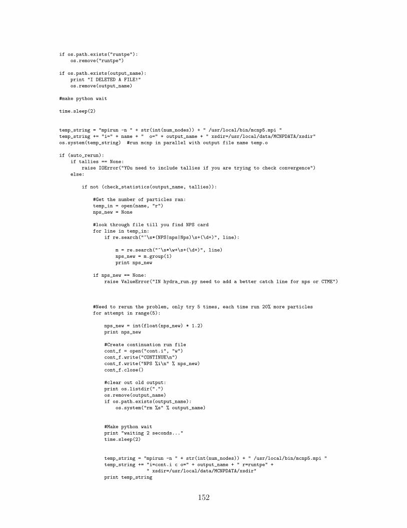
if os.path.exists("runtpe"):
os.remove("runtpe")
if os.path.exists(output_name):
print "I DELETED A FILE!"
os.remove(output_name)
#make python wait
time.sleep(2)
temp_string = "mpirun -n " + str(int(num_nodes)) + " /usr/local/bin/mcnp5.mpi "
temp_string += "i=" + name + " o=" + output_name + " xsdir=/usr/local/data/MCNPDATA/xsdir"
os.system(temp_string) #run mcnp in parallel with output file name temp.o
if (auto_rerun):
if tallies == None:
raise IOError("YOu need to include tallies if you are trying to check convergence")
else:
if not (check_statistics(output_name, tallies)):
#Get the number of particles ran:
temp_in = open(name, "r")
nps_new = None
#look through file till you find NPS card
for line in temp_in:
if re.search("^\s*(NPS|nps|Nps)\s+(\d+)", line):
m = re.search("^\s*\w+\s+(\d+)", line)
nps_new = m.group(1)
print nps_new
if nps_new == None:
raise ValueError("IN hydra_run.py need to add a better catch line for nps or CTME")
#Need to rerun the problem, only try 5 times, each time run 20% more particles
for attempt in range(5):
nps_new = int(float(nps_new) * 1.2)
print nps_new
#Create continuation run file
cont_f = open("cont.i", "w")
cont_f.write("CONTINUE\n")
cont_f.write("NPS %i\n" % nps_new)
cont_f.close()
#clear out old output:
print os.listdir(".")
os.remove(output_name)
if os.path.exists(output_name):
os.system("rm %s" % output_name)
#Make python wait
print "waiting 2 seconds..."
time.sleep(2)
temp_string = "mpirun -n " + str(int(num_nodes)) + " /usr/local/bin/mcnp5.mpi "
temp_string += "i=cont.i c o=" + output_name + " r=runtpe" +
" xsdir=/usr/local/data/MCNPDATA/xsdir"
print temp_string
152

os.system(temp_string)
os.remove("cont.i")
if check_statistics(output_name, tallies):
os.remove("runtpe")
break
if os.path.exists(output_name_final): #checks to make sure ouptut file name not already there
print "I DELETED A FILE!"
os.remove(output_name_final)
os.rename(output_name, output_name_final) #change name to name of input with .o extension
if os.path.exists(directory):
move_dir(output_name_final, directory)
move_dir(name, directory) #store files
eraser()
if flag:
os.chdir("..")
#Deletes all teh mcnp shit files
def eraser():
os.system("rm runt*")
#determine if hydra machine or not
def hydra_machine():
print "Is this a hydra (0) or PC (1) run?: "
hydra_flag = raw_input()
if (hydra_flag == "0"):
hydra_check = True
else:
hydra_check = False
return hydra_check
def main():
files = os.listdir(os.getcwd())
derp = []
for f in files:
if re.search(".i$", f):
derp.append(f)
files = list(derp)
num_nodes = raw_input("Input the number of nodes to use: ")
for name in files:
print "Running File "+name+", which is File %i of %i" % ((int(files.index(name))+1), len(files))
hydra_mcnp_run(name, "nodirectorychange", "same", num_nodes, auto_rerun = True, tallies = ["4"])
if __name__ == "__main__":
main()
153
run fom.py: Control Script for Simulated Data and FOM
calculations# This module runs all the other codes to generate responses and fom results
# In the main it calls fom_comparison_format which calculates Theta
#UPDATE: 081412: Added the ability to run multiple trials and average results with statistical error
#UPDATE: 103012: Added ability to keep going if it fails. Also in fom_comparison_format changed
#a bug that was adding incorrect amounts to the average.
#Added ability to rerun file and only redo those that failed by default. Adding a -new
#to command line execution will initiate an overwrite of the old file
import shutil # for copying files
import os # for directories and chmod etc.
import stat # for chmoding to user access
import subprocess # for running programs
import re # for regexps
import FOM_output #gets outputs and prints htem as response functions
import time # to tell program to wait
import fom_comparison_format
from sys import argv
import gc
#moves file to a directory OVERWRITING any files in the way
def move_dir(file_name, dir):
os.chdir(dir)
if os.path.exists(file_name):
os.remove(file_name)
os.chdir("..")
shutil.move(file_name, dir)
def makedirectory(dir):
if (not os.path.exists(dir)):
os.mkdir(dir)
os.chmod(dir, stat.S_IRWXU)
else:
os.chmod(dir, stat.S_IRWXU)
def main():
# - - - - - - - - - - -- - - - - -
#How many trials of results do you want to run and average?:
num_trials = 1000
nps = 2.E8 #number of histroies to scale to
#changeable filenames:
fom_name = "fom.exe"
resp_name = "simul_resp.exe"
src_str = "src_str.txt"
fom_output = "FOM.out"
#get the list of directories
directories = [] #list of directories that contain output files
completed_directories = [] #list of directories that have already been completed
#If list of completed directories already exists, read in names from file
if os.path.exists("completed_directories.txt"):
if len(argv) > 1:
if re.search("-n", argv[1]):
#Will make new files later
print "Creating new completed_directories file"
154
else:
comp_dir_file = open("completed_directories.txt", "r")
for line in comp_dir_file:
if len(line) > 0:
completed_directories.append(line.strip())
comp_dir_file.close()
comp_dir_file = open("completed_directories.txt", "a")
print "The following directories are complete: "
print completed_directories
time.sleep(1.5)
else:
comp_dir_file = open("completed_directories.txt", "w")
dir_list = os.listdir(os.getcwd())
for name in dir_list:
if re.search("Det\d+PE", name.strip()):
if os.path.isdir(name):
directories.append(name.strip())
#rip the outputs from the files in each directory
#The main function will return a list of all the files in each one
file_list = []
print directories
for dir in directories:
file_list.append(FOM_output.main(dir, scale=nps))
#create an initial ’irand’ file which is used for the simulated response data as a random number seed
if os.path.exists(’irand’):
os.remove(’irand’)
irand = open(’irand’,"w")
irand.write("73907\n")
irand.close()
makedirectory("FOM_outputs")
#open output file, if rerun (option "-n" not specified), then append to file, dont make new one,
#Else Make new one, also make new completed_directories file
if len(argv) > 1:
if re.search("-n", argv[1]):
outfile = open("FOM_outputs"+"/"+"FOM_comparison.out", "w")
comp_dir_file = open("completed_directories.txt", "w")
else:
outfile = open("FOM_outputs"+"/"+"FOM_comparison.out", "a")
first_time = True
for dir in directories:
#Skip directories that have already been completed
if dir in completed_directories:
continue
#Initialize instance of class. Each Class recieves the same output file, and when called to print will
#just print to the end of it
all_data = fom_comparison_format.all_data(outfile, dir+".fomout")
average_theta = []
print "Comparing data for geometry: %s... " % dir
for i in range(num_trials):
155

if i % int(0.1*num_trials) == 0:
print "Completed %.0f%% of %i trials" % (100*float(i)/float(num_trials), num_trials)
if i == 0:
shutil.copy(fom_name, dir)
shutil.copy(resp_name, dir)
shutil.copy(src_str, dir)
move_dir(’irand’, dir)
os.chdir(dir)
#run fom codes
if i % 900 == 0:
time.sleep(2)
try:
subprocess.check_call(resp_name)
subprocess.check_call(fom_name)
except:
print "HAD ONE FILE FAIL, DOES NOT AFFECT AVERAGE"
time.sleep(1.0)
continue
#change name of output and make copy in parent directory in folder "fom_results"
out_name_str = dir+".fomout"
if os.path.exists(out_name_str):
try:
os.remove(out_name_str)
except:
time.sleep(1.0)
print "Waiting to delete file: ", out_name_str
os.remove(out_name_str)
os.rename(fom_output, out_name_str)
#Get data
# - - - - - -- - - - - -- - - - - -- - -
all_data.parse()
average_theta.append(all_data.get_last_value(0))
if i == (num_trials - 1):
#delete duplicate files
os.remove(fom_name)
os.remove(resp_name)
os.remove(src_str)
shutil.move(’irand’,"..") #move current random number seed back to parent directory
shutil.copy(out_name_str, "../"+"FOM_outputs")
#return to parent directory
os.chdir("..")
else:
#Need to remove all files that are not being kept, except on last trial
try:
#os.remove("FOM.plt")
os.remove(out_name_str)
os.remove("simul_resp.out")
except:
try:
time.sleep(0.0001)
os.remove("simul_resp.out")
os.remove(out_name_str)
except:
continue
156

#averages output
averages_output = open("average.out","w")
for i in average_theta:
averages_output.write("%f\n" % i)
all_data.average_results()
if first_time:
first_time = False
fp = None
else:
fp = True
all_data.fprint(average=True, format=1, format_printed=fp)
#force so doesn’t reuse same one, seems to be a wierd bug elsewhere
del all_data
gc.collect()
#Write out completed directories to a file, skip these directories if no errors
comp_dir_file.write(dir+"\n")
#when done get rid of ’irand’ to not mess up the next time someone uses this code
os.remove(’irand’)
comp_dir_file.close()
if True:
main()
157
fom comparison format.py: Data Utility Class
# Load local modules
# ------------------------------------------------------------------------------------
import os
import re
# ------------------------------------------------------------------------------------
#UPDATE: July 11 2012
#Added ability to generate many responses and average results
class all_data(object):
"""Each instance of this class contains all the data for all of the responses for one particular geometry.
Averaging can be done more easily this way inside the class"""
# - - - - - - -- - - - - - -- - - - - - -- - - - - - -- - - - - - -- - - - - - -- - - - - - -
def __init__(self, outfile, infile_handle):
#Get rid of the old data
self.clear()
self.outfile = outfile
if self.outfile.closed:
raise ValueError("Somehow you closed the file you passed in")
self.file_name = infile_handle
return None
# - - - - - - -- - - - - - -- - - - - - -- - - - - - -- - - - - - -- - - - - - -- - - - - - -
def clear(self):
"""Clears and initializes all data"""
self.strength = []
self.difference = []
self.lowest_fom = []
self.original_source = []
self.closest_template = []
self.smallest_template = []
self.avg_eff = []
self.not_matches = []
self.outfile = None
self.geometry = None
self.diff_std_dev = None
self.averaged = False
self.format_printed = False
self.functions_list = ["functions_list", "clear", "parse", "initialize_lists", "fprint",
"outfile", "file_name", "geometry", "average_results", "averaged",
"diff_std_dev","format_printed"]
self.file_name = None
return None
# - - - - - - -- - - - - - -- - - - - - -- - - - - - -- - - - - - -- - - - - - -- - - - - - -
def initialize_lists(self, num_strengths):
"""makes all attributes be lists of the appropriate length so u can store data for each source strenght"""
attributes = dir(self)
#Get rid of the default functions
temp_list = []
for i in attributes:
158
if not search_for(i, "__\S+__"):
if i not in self.functions_list:
temp_list.append(i)
else:
continue
attributes = temp_list
#Initialize each list
for j in attributes:
exec("self.%s = [ [] for i in range(num_strengths)] " % (j))
return None
# - - - - - - -- - - - - - -- - - - - - -- - - - - - -- - - - - - -- - - - - - -- - - - - - -
def parse(self):
"""Reads in the data for a single geometry/configuration folder, and appends sorted data of it to each
list. You can read in multiple sampling of the same geometry, but not different files
The way it works is each item (e.g.) efficiency has a list for each source strength, then with in
each source strength is a list for each trial. The last member is made the average eventually"""
#open file passed in during init
print "comparing data for:", self.file_name
if self.file_name == None:
raise ValueError("need to pass in a filename to be parsed")
if (not search_for(self.file_name, ".fomout")):
print self.file_name, "had no data"
return None
file_handle = open(self.file_name, "r")
#Local variables.
new_strength_flag = False
temp_list = []
counter_flag = 0
first_time_flag = True
efficiency = []
strength = []
difference = []
lowest_fom = []
closest_template = []
smallest_template = []
original_source = []
avg_eff = []
master_list = [] #Each member of list is for a specific energy
for line in file_handle: #loop through all the lines in each file
line_data = line.split()
if search_for(line, ’c\*’):
#Start of a new set of FOM data, figure out the actual source:
source = line.split()[3]
elif search_for(line, "total incident"):
#Find and get the efficiency for this source strength
159
new_strength_flag = True
counter_flag = 0
#Reinitialize list for storing the first and second smallest FOM’s:
temp_list = []
efficiency.append(line_data[14].rstrip(’%’))
strength.append(line_data[10].strip())
elif search_for(line, ’c--+’):
#All data has been read in for a particular source, now store it and reset lists
if first_time_flag == True:
#initialize the list of all results to have a slot for each source strength
for i in strength:
master_list.append([])
avg_eff.append([])
first_time_flag = False
for each in range(len(strength)): #store each of the results, for each strength, then compare
data_temp = [difference[each], strength[each], lowest_fom[each], original_source[each],
smallest_template[each], closest_template[each], efficiency[each]]
master_list[each].append(data_temp)
avg_eff[each].append(efficiency[each])
# Organized by [difference[2], strength[2], smallest_template[2],
# closest_template[2], original_source[2], lowest_fom[2], efficiency[2]
new_strength_flag = False
temp_list = []
counter_flag = 0
efficiency = []
strength = []
difference = []
lowest_fom = []
closest_template = []
smallest_template = []
original_source = []
elif new_strength_flag:
#Data for a new source strength
#Counter flag is what line you are on in data for a particular source
if (counter_flag <1):
#Skip first line because it just contains the number of counts in each detector
counter_flag +=1
elif counter_flag < 3 :
#Read in the top two lowest FOM scores
if (search_for(line, "--ERROR:")): #when zero coutns make sure it catchs it by
#setting diff to zero
temp_list = [[0,0,0],[0,0,0]]
temp_list[1][1] = 1.
temp_list[0][1] = 1.
temp_list[1][2] = 1.
temp_list[0][0] = "ERROR: ZERO COUNTS"
temp_list[1][0] = "ERROR: ZERO COUNTSnUIMBER2"
counter_flag = 80
temp_list.append([line_data[0], line_data[2], line_data[4]])
160
counter_flag += 1
else:
#have the data you need:
#Templist[i] = [source type, FOM, std_dev]
if (float(temp_list[1][1]) < 0.0001):
#Make sure FOM not zero
diff = 0.0
source = "False Data, No counts in bins other than normaliz"
else:
diff = float(temp_list[1][1])-float(temp_list[0][1])
diff = diff/float(temp_list[1][2])
#Store data locally:
difference.append(diff)
original_source.append(source)
lowest_fom.append(temp_list[0][1])
smallest_template.append(temp_list[0][0])
closest_template.append(temp_list[1][0])
temp_list = []
new_strength_flag = False
#Sort all the data for this file and append to the instance’s lists
temp_master = []
for each in range(len(master_list)):
temp_master.append(sorted(master_list[each], key = lambda diff: diff[0]))
#Compute the average efficiency
asum = 0.0
for num in avg_eff[each]:
asum = asum + float(num)
avg_eff[each] = asum/float(len(avg_eff[each]))
master_list = list(temp_master)
#if necessary initialize lists to be smae length as source strengths:
if self.strength == []:
self.initialize_lists(len(master_list))
#determine the number of misses there are and store data:
for i in range(len(master_list)):
if self.not_matches[i] == []:
self.not_matches[i] = 0
else:
for data in master_list[i]:
if not search_for(data[4], data[3].rstrip(".i")) or data[0] < 0.0000000001:
master_list[i][master_list[i].index(data)][0] = 0.0
#Not a match
# print "adding to not matches"
self.not_matches[i] +=1
break #DEBUG TODO this break statemetn is for if you want to know that it failed
# in one "trial", somewhere, remove to know fails of all samples of all
# sources
else:
continue
161
#Store the worse case data:
for i in range(len(master_list)):
self.avg_eff[i].append(avg_eff[i])
self.difference[i].append(master_list[i][0][0])
self.strength[i].append(master_list[i][0][1])
self.lowest_fom[i].append(master_list[i][0][2])
self.smallest_template[i].append(master_list[i][0][4])
self.original_source[i].append(master_list[i][0][3])
self.closest_template[i].append(master_list[i][0][5])
return None
# - - - - - - - - - - - - - - - - - - - - - - - - - - - - - - - - - - - - - - - - - - - - - - - - - - - - -
def fprint(self, idx=None, average=None, format=None, format_printed=None):
"""Method that prints out to file nice and pretty. Only prints for case (geometry) specified by idx,
but prints for all source strengths"""
"""format is used to print in special formats. Format == 1 prints it so that all of the data from
the difference are printed for a single chi_sq value"""
#Default to self.averaged:
if average == None:
average = self.averaged
if format_printed != None:
self.format_printed = format_printed
#If not an averaged result
if not average:
self.outfile.write("\nc------------------------------")
self.outfile.write("\nc *** Geometry is: %s \n" % (self.file_name.strip()))
#Default print the first one
if idx == None:
idx = 0
self.outfile.write(" Source_Strength Difference(in sigma’s) SmallestFOM"
+" Source Number Misses Closest_Template AvgEfficiency")
for i in range(len(self.strength)):
self.outfile.write("\n %13s %19.4f %19s %15s %11i %23s %18.4f%s" % (self.strength[i][idx],
float(self.difference[i][idx]), self.lowest_fom[i][idx], self.original_source[i][idx],
self.not_matches[i], self.closest_template[i][idx], (self.avg_eff[i][idx]),"%"))
else:
#If is an averaged result, just print the last one cause thats where the average is
idx = -1
if format == None or format == 0:
self.outfile.write("\nc------------------------------")
self.outfile.write("\nc *** Geometry is: %s \n" % (self.file_name.strip()))
self.outfile.write("Averaged Result:\n")
self.outfile.write("Source_Strength Difference(in sigma’s) Std Dev of Difference"
+"SmallestFOM Number Misses AvgEfficiency")
for i in range(len(self.strength)):
self.outfile.write("\n %13s %19.4f %19.4f %18.3f %16.3f %18.4f%s" % (self.strength[i][idx],
float(self.difference[i][idx]), self.diff_std_dev[i], float(self.lowest_fom[i][idx]),
float(self.not_matches[i]), (self.avg_eff[i][idx]),"%"))
162
elif format == 1:
#print the diference and the errors for each source strength in a column
#for all thickness and such. Also print the thicknesses;
if not self.format_printed:
self.outfile.write(" GeometryName Radius No._Detectors Thickness ")
#print the source strengths:
for i in self.strength:
self.outfile.write("Str:%8s_(n’s) sig. number_miss " % i[0])
self.outfile.write("\n")
self.format_printed = True
#get the number of detectors and thickness:
m = re.search("Det(\d+)PE(\d+\.\d+)R(\d+\.\d+)\.fomout", self.file_name.strip())
m_num_det = float(m.group(1))
m_poly_thick = float(m.group(2))
m_radius = float(m.group(3))
#print name, geometry, etc.
self.outfile.write("%21s%8.2f%9i%14.2f " % (self.file_name.strip(), m_radius, m_num_det,
m_poly_thick))
for i in range(len(self.strength)):
self.outfile.write("%13.4f%11.4f%12.4f" % (self.difference[i][idx], self.diff_std_dev[i],
self.not_matches[i]))
self.outfile.write("\n")
else:
raise ValueError("Invalid format entry")
return None
# - - - - - - - - - - - - - - - - - - - - - - - - - - - - - - - - - - - - - - - - - - - - - - -
def average_results(self):
"""Method that averages all results and stores the average to the results as the last in the list"""
if self.averaged == True:
raise ValueError("already averaged, wont work right")
attributes = dir(self)
#local average values
avg_eff = [ 0. for i in range(len(self.strength))]
diff = [ 0. for i in range(len(self.strength))]
lowest_fom = [ 0. for i in range(len(self.strength))]
diff_sq = [ 0. for i in range(len(self.strength))]
not_matches = [ 0 for i in range(len(self.strength))]
std_dev = []
for i in range(len(self.not_matches)):
self.not_matches[i] = float(self.not_matches[i])
self.not_matches[i] /= float(len(self.strength[i]))
#compute sum of values and square
for idx in range(len(self.strength)):
num_trials = len(self.avg_eff[idx])
163
for i in range(len(self.avg_eff[idx])):
avg_eff[idx] += self.avg_eff[idx][i]
diff[idx] += self.difference[idx][i]
diff_sq[idx] += self.difference[idx][i]*self.difference[idx][i]
lowest_fom[idx] += float(self.lowest_fom[idx][i])
#compute average
avg_eff[idx] /= num_trials
diff[idx] /= num_trials
diff_sq[idx] /= num_trials
if num_trials != 1:
std_dev.append(1./(num_trials-1.)*(diff_sq[idx] - diff[idx]*diff[idx]))
else:
std_dev.append(1./(num_trials)*(diff_sq[idx] - diff[idx]*diff[idx]))
#store all average results as last member of list
self.diff_std_dev = std_dev
for src in range(len(self.strength)):
self.difference[src].append(diff[src])
self.avg_eff[src].append(avg_eff[src])
self.lowest_fom.append(lowest_fom[src])
self.averaged=True
return None
#searchs a line for a string, returns true if found, else false
def search_for(line, string):
pattern = re.compile(string)
if (pattern.search(line)):
return True
else:
return False
if __name__ == "__main__":
file = open("test.txt", "a")
os.chdir("FOM_outputs")
a = all_data(file, "Det6PE4.0R10.0.fomout")
a.parse()
os.chdir("..")
a.fprint(idx=0)
a.average_results()
print a.averaged
a.fprint(average=True)
a.average_results()
file.close()
# os.remove("test.txt")
164

master file.fom: Sample Output from FOM output.py’100ev’
11 6.8 ! number of detectors, radius of spectrometer
4.07152E-07 0.0250 ! r_i, sigma(r_i)/r_i
2.36026E-06 0.0235
5.25792E-07 0.0304
4.86122E-08 0.0637
3.87641E-09 0.2023
0.00000E+00 0.0000
0.00000E+00 0.0000
0.00000E+00 0.0000
0.00000E+00 0.0000
0.00000E+00 0.0000
0.00000E+00 0.0000
’ambe’
11 6.8
9.24320E-08 0.0572
8.26495E-07 0.0429
6.06992E-07 0.0408
2.93210E-07 0.0454
1.58648E-07 0.0501
1.11427E-07 0.0475
6.86984E-08 0.0474
4.63191E-08 0.0436
2.88369E-08 0.0405
1.71930E-08 0.0412
7.55912E-09 0.0573
’cf252mcnp’
11 6.8
5.20806E-08 0.0964
5.22608E-07 0.0511
5.91422E-07 0.0430
4.38491E-07 0.0409
2.64141E-07 0.0409
1.54190E-07 0.0420
8.01043E-08 0.0448
4.74482E-08 0.0437
2.73162E-08 0.0449
1.48358E-08 0.0440
5.94480E-09 0.0523
’cfd2oN’
11 6.8
3.36993E-07 0.0291
1.81081E-06 0.0272
6.92907E-07 0.0294
1.91853E-07 0.0338
6.97646E-08 0.0373
3.21269E-08 0.0434
1.85437E-08 0.0473
1.10869E-08 0.0561
5.49360E-09 0.0579
3.42547E-09 0.0544
1.39792E-09 0.0632
’fusionN’
11 6.8
9.17220E-09 0.1917
1.06044E-07 0.1095
1.39183E-07 0.0868
1.61640E-07 0.0848
1.38673E-07 0.0805
1.06838E-07 0.0808
9.37919E-08 0.0864
8.28473E-08 0.0817
5.87632E-08 0.0745
4.38710E-08 0.0836
2.08117E-08 0.1000
165

simul resp.f90: Source Code for Generating Simulated
ResponsesPROGRAM simul_resp
! Program to generate simulated count data from response functions
! Same as SIMUL but response functions are read from a file and not
! defined by DATA statements
IMPLICIT NONE
REAL, ALLOCATABLE, DIMENSION(:) :: resp, ecount, src
INTEGER, ALLOCATABLE, DIMENSION(:) :: ncount
CHARACTER(len=40) :: stype
REAL, PARAMETER :: PI = 3.14159265
COMMON/RANCOM/ISEED !Random Num_seed
INTEGER :: open_error !I/O STATUS
CHARACTER (len=20) :: output_name, infile_name !output file name
INTEGER :: STATUS !For dynamic memory status
INTEGER :: I, isrc, num_src, idet, iround, iseed!loop counters
REAL :: x, sig, cyl_rad, source
INTEGER :: n, num_det
! READ IN THE SOURCE INFORMATION FROM A FILE
OPEN(555,FILE=’src_str.txt’,STATUS=’OLD’,ACTION=’READ’, IOSTAT=open_error)
IF (open_error /= 0) THEN
STOP "Can’t find the src_str.txt file for source strengths"
END IF
READ (555,*) num_src
ALLOCATE(src(num_src), STAT=STATUS) !allocate memory for number of sources
IF (status /= 0) THEN
STOP "Problem allocating memory"
END IF
DO I=1,num_src,1
READ(555,*) src(I)
END DO
!Read iseed from a file so as not to use same random num every time
OPEN(UNIT=556,FILE=’irand’,STATUS=’OLD’,ACTION=’READ’, IOSTAT=open_error)
IF (open_error /= 0) THEN
write(*,*) "No file found, use default seed of 73907"
iseed = 73907
ELSE
READ(556,*) iseed
CLOSE(UNIT=556)
END IF
OPEN(11,FILE=’simul_resp.out’,STATUS=’UNKNOWN’)
!-- Begin loop to process all response functions
output_name = "master_file.fom"
OPEN (UNIT=10, FILE=output_name, STATUS=’UNKNOWN’, ACTION=’READ’, &
&IOSTAT=open_error)
IF (open_error /= 0) THEN
STOP "No response function, (master_file.fomin), file"
END IF
98 READ(10,*,END=99) stype
READ(10,*) num_det, cyl_rad
ALLOCATE(resp(num_det), ncount(num_det), ecount(num_det), STAT=STATUS)
IF (status /= 0) THEN
STOP "Problem allocating memory for detector arrays"
END IF
166
DO 97 i=1,num_det
READ(10,*) resp(i)
97 CONTINUE
!** process both spectra
stype= ’ ’’ ’//’Source is ’//stype
WRITE(11,50) stype,’ ’’ ’
WRITE(11,53) num_det, num_src, cyl_rad
53 FORMAT(1x, 2I5, 1F10.1)
50 FORMAT(A40,A3)
!-- loop over all source strengths
DO 20 isrc=1,num_src
!Normalize the responses to per area of 10cm^2. i.e., if you have
!an area of 10cm^2, then the total source is what is read in
source = src(isrc)*cyl_rad*cyl_rad/100.
!-- loop over all detector locations
DO 30 idet=1,num_det
ecount(idet)=resp(idet)*source
!-- sample from expected counts
IF (ecount(idet).LE.0.01) THEN
ncount(idet)=0
ELSEIF (ecount(idet) .GT. 20.) THEN
sig=SQRT(ecount(idet))
CALL Normal(ecount(idet),sig,x)
! -- round x to nearest integer
n=INT(x)
iround = INT(2*x-2*n)
ncount(idet)=n+iround
ELSE
CALL Poiss(ecount(idet),n)
ncount(idet)=n
ENDIF
30 CONTINUE
WRITE(11,52) source,(ncount(i),i=1,num_det)
52 FORMAT(1X, 1g14.4, 15I12)
20 CONTINUE
DEALLOCATE(resp, ncount, ecount)
GOTO 98
99 CLOSE(11)
DEALLOCATE(src)
!write the randomnumber seed to the directory
OPEN(UNIT=666,FILE=’irand’,STATUS=’REPLACE’, ACTION=’WRITE’, IOSTAT=open_error)
WRITE(666,*) iseed
CLOSE(UNIT=666)
END PROGRAM simul_resp
SUBROUTINE Normal(m,sig,x)
!---------------------------------------------------------------------
! Generates a random sample x from a normal N(m,sig) distribution
! using the Box-Muller method.
!
! INPUT: m = the mean of the Gaussian distribution
! sig = the standard deviation of the Gaussian distribution
!
! OUTPUT: x = a random sample from the Gaussian distribution
!
! NOTE: Although, in general, m and sig can be independent, for
! counting data m = sig^2
!---------------------------------------------------------------------
REAL m
rho1 = FLTRN()
rho2 = FLTRN()
167
y = SQRT(-2.*log(rho1))*COS(6.283185*rho2)
x = sig*y + m
RETURN
END
SUBROUTINE Poiss(m,n)
!---------------------------------------------------------------------
! Generates a random sample n from a Poisson distribution with mean m
!---------------------------------------------------------------------
REAL m,lnm
!-- initialize
rho = FLTRN()
n=0
em = EXP(-m)
fn = em
lnm = LOG(m)
FFn = fn
!-- use inverse CDF method
DO 10 i=1,45
IF (rho .GT. FFn) THEN
n=n+1
fn = EXP(n*lnm - m - gammln(FLOAT(n+1)))
FFn = FFn + fn
ELSE
RETURN
ENDIF
10 CONTINUE
WRITE(*,*)’ WARNING: Poisson sampling failed’
END
FUNCTION gammln(xx)
!----------------------------------------------------------------------
! Returns value of ln[Gamma(xx)]. From "Numerical Recipes"
!----------------------------------------------------------------------
REAL gammln,xx
INTEGER j
DOUBLE PRECISION ser,stp,tmp,x,y,cof(6)
SAVE cof,stp
DATA cof,stp/76.18009172947146d0,-86.50532032941677d0, &
& 24.01409824083091d0,-1.231739572450155d0,.1208650973866179d-2, &
& -.5395239384953d-5,2.5066282746310005d0/
x=xx
y=x
tmp=x+5.5d0
tmp=(x+0.5d0)*log(tmp)-tmp
ser=1.000000000190015d0
DO 10 j=1,6
y=y+1.d0
ser=ser+cof(j)/y
10 CONTINUE
gammln=tmp+log(stp*ser/x)
RETURN
END
REAL FUNCTION FLTRN()
!---------------------------------------------------------------------
! PURPOSE: Returns a single precision floating point random
! number in the open interval (0,1).
! Works on any system for which the maximum value
! of an integer variable is 2**31-1 or larger.
!
! ARGUMENTS: none (ISEED the seed number is kept in COMMON)
!
168

! METHOD: Minimal standard generator as specified in the article
! S.K. Park and K.W. Miller, "Random Number Generators:
! Good Ones are Hard to Find", Comm. ACM, vol. 31, no. 10,
! October 1988.
!---------------------------------------------------------------------
INTEGER a,m,q,r,lo,hi,test,iseed
REAL minv
COMMON/RANCOM/ISEED
PARAMETER(a=16807,m=2147483647,q=127773,r=2836)
PARAMETER(minv=4.6566129E-10)
hi = iseed/q
lo = MOD(iseed,q)
test = a*lo-r*hi
IF(test .GT. 0) THEN
iseed = test
ELSE
iseed = test + m
ENDIF
FLTRN = minv*REAL(iseed)
RETURN
END
169

fom.f90: Source Code for Computing FOM Values!******* Program for comparing a measured spectrometer response to templates
! The number 30 throughout is max number of different sources
! that are being simulated
!UPDATE 71112: Added ability to average results
PROGRAM fom_042412
IMPLICIT NONE
INTEGER, ALLOCATABLE, DIMENSION(:) :: ncount
REAL, ALLOCATABLE, DIMENSION(:) :: RR,sig2c
REAL, ALLOCATABLE, DIMENSION(:, :) :: rel
REAL, DIMENSION(30) :: fom,fom2,sigfom
REAL, DIMENSION(30,30) :: SS,sig2S, resp
CHARACTER(LEN=72) :: templ(30),templ2(30),label
INTEGER :: norm, nsrc, ndet,j,i,status,nresp
INTEGER :: nset, nsum, cnorm
REAL :: r2norm, Snorm, src, cyl_rad, eff
!** analysis parameters
norm = 2 !which detector to normalize to
!default is 10, radius of the spectrometer
!get number of source strengths
OPEN(UNIT=512,FILE=’simul_resp.out’,ACTION=’READ’,STATUS=’OLD’)
READ(512,*) label, ndet, nsrc !lable and ndet are just dummys here
CLOSE(UNIT=512)
!** open input/output files
OPEN(10,FILE=’simul_resp.out’,STATUS=’OLD’)
OPEN(11,FILE=’master_file.fom’,STATUS=’OLD’)
OPEN(12,FILE=’FOM.out’,STATUS=’UNKNOWN’)
OPEN(13,FILE=’FOM.plt’,STATUS=’UNKNOWN’)
!-- read in all templates and form ratios for the response functions
j=0
!-- loop to read response functions
40 j=j+1
READ(11,*,END=100) templ(j)
templ2(j)=templ(j)
READ(11,*) ndet, cyl_rad
ALLOCATE(RR(ndet), ncount(ndet), rel(30,ndet),&
&STAT=status)
IF (status /= 0) THEN
STOP "Problem allocating memory for detector arrays"
END IF
DO 15 i=1,ndet
READ(11,*) resp(j,i),rel(j,i)
15 CONTINUE
!-- calc ratios and variances
Snorm = resp(j,norm)
r2norm = rel(j,norm)**2
DO 16 i=1,ndet
SS(j,i) = LOG(resp(j,i)/Snorm)
sig2S(j,i) = (rel(j,i)**2 + r2norm)*100./(cyl_rad*cyl_rad)
16 CONTINUE
nresp=j
! DEALLOCATE MEMORY
DEALLOCATE(RR, ncount, rel,&
&)
GOTO 40
!-- big loop to read and process simulated count data
!** read in spectrometer count data
170

100 READ(10,*,END=300) label
READ(10,*) ndet, nsrc, cyl_rad
WRITE(12,31) label
WRITE(13,31) label
31 FORMAT( //’c****** ’,(A))
!Allocate memory
ALLOCATE(ncount(ndet), RR(ndet), sig2c(ndet))
nset=0
99 READ(10,306) src, (ncount(i),i=1,ndet)
306 FORMAT(1x, 1E14.4, 5000I12)
!-- find total number of counts
nsum=0
DO 35 i=1,ndet
nsum=nsum + ncount(i)
35 CONTINUE
eff = float(nsum)/(src)*100.
WRITE(12,38) nsum,src,eff,(ncount(i),i=1,ndet)
WRITE(13,34) label,nsum,(ncount(i),i=1,ndet)
34 FORMAT(/(A),/&
& ’Simulated count data: total counts = ’,I10,/4000I8)
38 FORMAT(/’Simulated count data: total counts = ’,I10,’ total incident&
& neutrons= ’,ES10.1,’ total efficiency = ’,F7.4, ’%’/40001I8)
nset=nset+1
!-- check that normalization counts are not zero
IF (ncount(norm).EQ.0) THEN
WRITE(12,36)norm
WRITE(12,333)
WRITE(13,333)
IF (nset.EQ.nsrc) THEN
DEALLOCATE(ncount, RR, sig2c)
WRITE(12,333)
WRITE(13,333)
GOTO 100
ELSE
GOTO 99
ENDIF
ENDIF
36 FORMAT(’--ERROR: normalization detector’,I2,’ has zero counts’)
!-- calculate log of ratios and stnd dev. for count data
cnorm = ncount(norm)
DO 11 i=1,ndet
IF (ncount(i).GT.0) THEN
sig2c(i) = 1./FLOAT(ncount(i)) + 1./FLOAT(cnorm) !Corrected
RR(i) = LOG(1.*ncount(i)/FLOAT(cnorm))
ELSE
sig2c(i)=0.0
RR(i) = LOG(1./cnorm)
ENDIF
11 CONTINUE
!** compare data to all response functions -- calc FOM and stnd dev.
DO 10 j=1,nresp
!-- calc figure of merit (FOM)
fom(j)=0.0
DO 30 i=1,ndet
IF((resp(j,i).GT.1E-15).AND.(ncount(i).GT.0)) THEN
fom(j)=fom(j)+(RR(i)-SS(j,i))**2/(sig2S(j,i) + sig2c(i))
ENDIF
30 CONTINUE
sigfom(j)=2*SQRT(fom(j))
fom2(j)=fom(j)
171
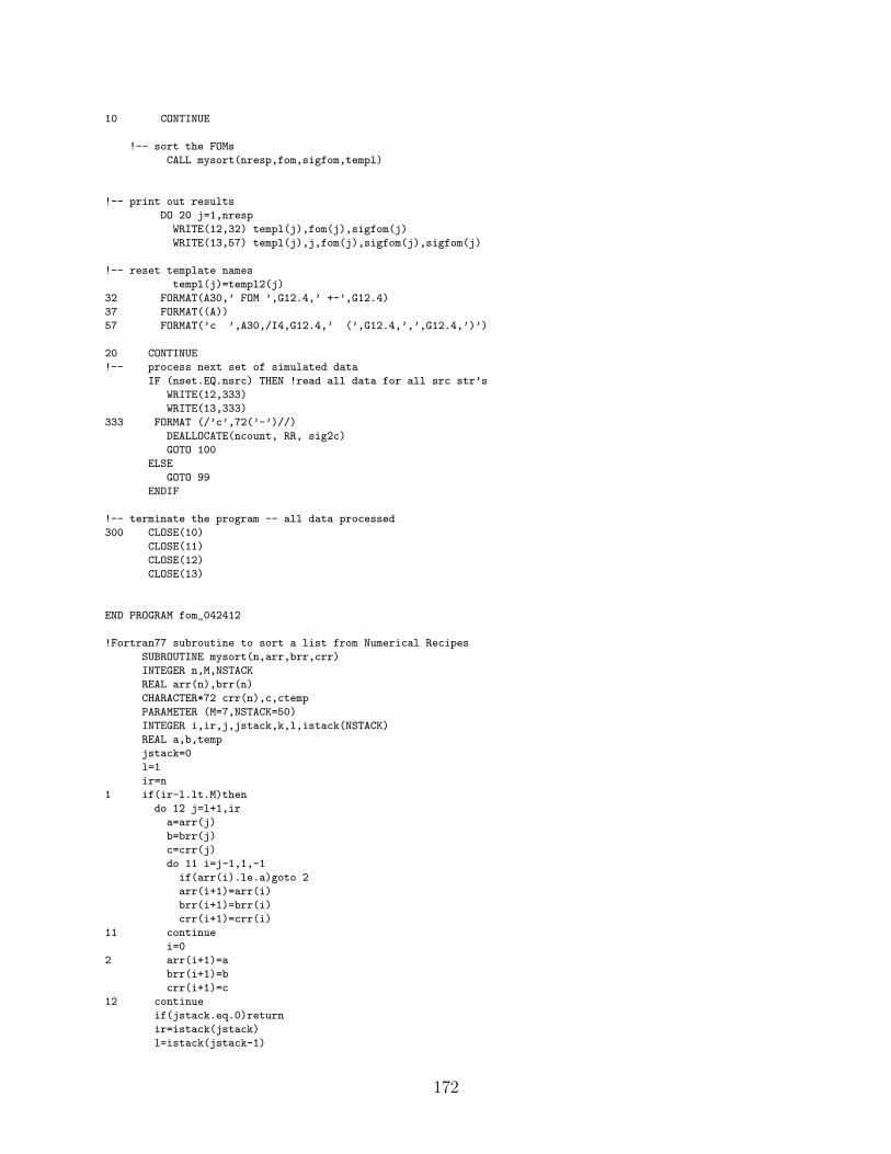
10 CONTINUE
!-- sort the FOMs
CALL mysort(nresp,fom,sigfom,templ)
!-- print out results
DO 20 j=1,nresp
WRITE(12,32) templ(j),fom(j),sigfom(j)
WRITE(13,57) templ(j),j,fom(j),sigfom(j),sigfom(j)
!-- reset template names
templ(j)=templ2(j)
32 FORMAT(A30,’ FOM ’,G12.4,’ +-’,G12.4)
37 FORMAT((A))
57 FORMAT(’c ’,A30,/I4,G12.4,’ (’,G12.4,’,’,G12.4,’)’)
20 CONTINUE
!-- process next set of simulated data
IF (nset.EQ.nsrc) THEN !read all data for all src str’s
WRITE(12,333)
WRITE(13,333)
333 FORMAT (/’c’,72(’-’)//)
DEALLOCATE(ncount, RR, sig2c)
GOTO 100
ELSE
GOTO 99
ENDIF
!-- terminate the program -- all data processed
300 CLOSE(10)
CLOSE(11)
CLOSE(12)
CLOSE(13)
END PROGRAM fom_042412
!Fortran77 subroutine to sort a list from Numerical Recipes
SUBROUTINE mysort(n,arr,brr,crr)
INTEGER n,M,NSTACK
REAL arr(n),brr(n)
CHARACTER*72 crr(n),c,ctemp
PARAMETER (M=7,NSTACK=50)
INTEGER i,ir,j,jstack,k,l,istack(NSTACK)
REAL a,b,temp
jstack=0
l=1
ir=n
1 if(ir-l.lt.M)then
do 12 j=l+1,ir
a=arr(j)
b=brr(j)
c=crr(j)
do 11 i=j-1,1,-1
if(arr(i).le.a)goto 2
arr(i+1)=arr(i)
brr(i+1)=brr(i)
crr(i+1)=crr(i)
11 continue
i=0
2 arr(i+1)=a
brr(i+1)=b
crr(i+1)=c
12 continue
if(jstack.eq.0)return
ir=istack(jstack)
l=istack(jstack-1)
172

jstack=jstack-2
else
k=(l+ir)/2
temp=arr(k)
arr(k)=arr(l+1)
arr(l+1)=temp
temp=brr(k)
brr(k)=brr(l+1)
brr(l+1)=temp
ctemp=crr(k)
crr(k)=crr(l+1)
crr(l+1)=ctemp
if(arr(l+1).gt.arr(ir))then
temp=arr(l+1)
arr(l+1)=arr(ir)
arr(ir)=temp
temp=brr(l+1)
brr(l+1)=brr(ir)
brr(ir)=temp
ctemp=crr(l+1)
crr(l+1)=crr(ir)
crr(ir)=ctemp
endif
if(arr(l).gt.arr(ir))then
temp=arr(l)
arr(l)=arr(ir)
arr(ir)=temp
temp=brr(l)
brr(l)=brr(ir)
brr(ir)=temp
ctemp=crr(l)
crr(l)=crr(ir)
crr(ir)=ctemp
endif
if(arr(l+1).gt.arr(l))then
temp=arr(l+1)
arr(l+1)=arr(l)
arr(l)=temp
temp=brr(l+1)
brr(l+1)=brr(l)
brr(l)=temp
ctemp=crr(l+1)
crr(l+1)=crr(l)
crr(l)=ctemp
endif
i=l+1
j=ir
a=arr(l)
b=brr(l)
c=crr(l)
3 continue
i=i+1
if(arr(i).lt.a)goto 3
4 continue
j=j-1
if(arr(j).gt.a)goto 4
if(j.lt.i)goto 5
temp=arr(i)
arr(i)=arr(j)
arr(j)=temp
temp=brr(i)
brr(i)=brr(j)
brr(j)=temp
ctemp=crr(i)
crr(i)=crr(j)
crr(j)=ctemp
goto 3
5 arr(l)=arr(j)
173

arr(j)=a
brr(l)=brr(j)
brr(j)=b
crr(l)=crr(j)
crr(j)=c
jstack=jstack+2
if(jstack.gt.NSTACK) STOP ’NSTACK too small in sort2’
if(ir-i+1.ge.j-l)then
istack(jstack)=ir
istack(jstack-1)=i
ir=j-1
else
istack(jstack)=j-1
istack(jstack-1)=l
l=i
endif
endif
goto 1
END
174
Appendix C
Spectrometer MCNP Files
Description Page
MCNP5 file for a uniform beam of 252Cf irradiat-ing a spectrometer in a void.
176
MCNP5 file for a point source of 252Cf irradiatinga spectrometer in an enclosed room with shadowshield included.
179
MCNP6 input file for verifying spectrometer re-sponse from 252.Cf
183
175
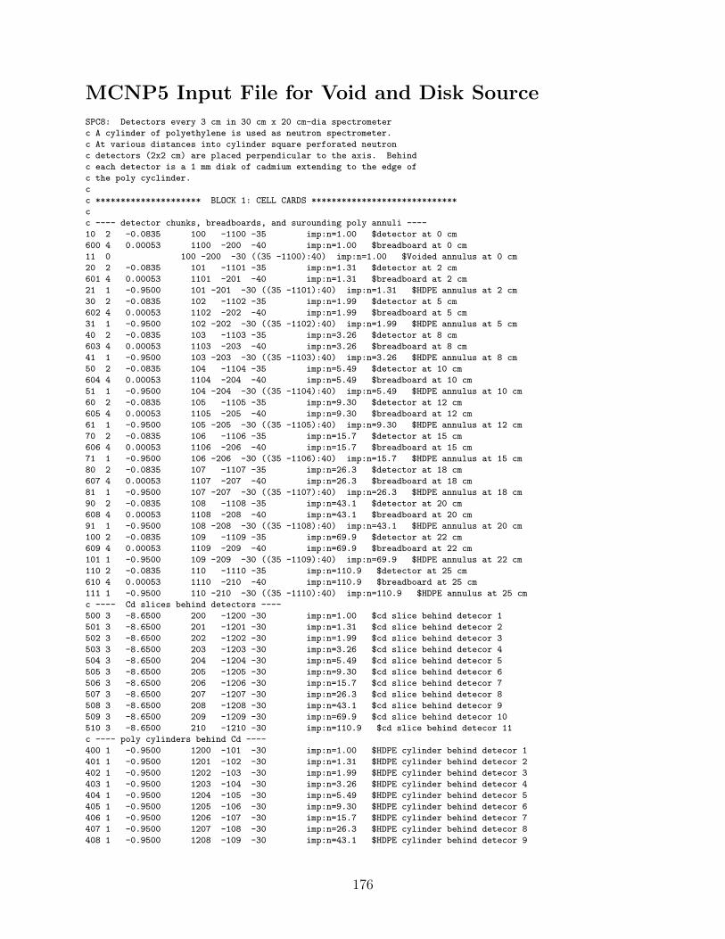
MCNP5 Input File for Void and Disk SourceSPC8: Detectors every 3 cm in 30 cm x 20 cm-dia spectrometer
c A cylinder of polyethylene is used as neutron spectrometer.
c At various distances into cylinder square perforated neutron
c detectors (2x2 cm) are placed perpendicular to the axis. Behind
c each detector is a 1 mm disk of cadmium extending to the edge of
c the poly cyclinder.
c
c ********************* BLOCK 1: CELL CARDS *****************************
c
c ---- detector chunks, breadboards, and surounding poly annuli ----
10 2 -0.0835 100 -1100 -35 imp:n=1.00 $detector at 0 cm
600 4 0.00053 1100 -200 -40 imp:n=1.00 $breadboard at 0 cm
11 0 100 -200 -30 ((35 -1100):40) imp:n=1.00 $Voided annulus at 0 cm
20 2 -0.0835 101 -1101 -35 imp:n=1.31 $detector at 2 cm
601 4 0.00053 1101 -201 -40 imp:n=1.31 $breadboard at 2 cm
21 1 -0.9500 101 -201 -30 ((35 -1101):40) imp:n=1.31 $HDPE annulus at 2 cm
30 2 -0.0835 102 -1102 -35 imp:n=1.99 $detector at 5 cm
602 4 0.00053 1102 -202 -40 imp:n=1.99 $breadboard at 5 cm
31 1 -0.9500 102 -202 -30 ((35 -1102):40) imp:n=1.99 $HDPE annulus at 5 cm
40 2 -0.0835 103 -1103 -35 imp:n=3.26 $detector at 8 cm
603 4 0.00053 1103 -203 -40 imp:n=3.26 $breadboard at 8 cm
41 1 -0.9500 103 -203 -30 ((35 -1103):40) imp:n=3.26 $HDPE annulus at 8 cm
50 2 -0.0835 104 -1104 -35 imp:n=5.49 $detector at 10 cm
604 4 0.00053 1104 -204 -40 imp:n=5.49 $breadboard at 10 cm
51 1 -0.9500 104 -204 -30 ((35 -1104):40) imp:n=5.49 $HDPE annulus at 10 cm
60 2 -0.0835 105 -1105 -35 imp:n=9.30 $detector at 12 cm
605 4 0.00053 1105 -205 -40 imp:n=9.30 $breadboard at 12 cm
61 1 -0.9500 105 -205 -30 ((35 -1105):40) imp:n=9.30 $HDPE annulus at 12 cm
70 2 -0.0835 106 -1106 -35 imp:n=15.7 $detector at 15 cm
606 4 0.00053 1106 -206 -40 imp:n=15.7 $breadboard at 15 cm
71 1 -0.9500 106 -206 -30 ((35 -1106):40) imp:n=15.7 $HDPE annulus at 15 cm
80 2 -0.0835 107 -1107 -35 imp:n=26.3 $detector at 18 cm
607 4 0.00053 1107 -207 -40 imp:n=26.3 $breadboard at 18 cm
81 1 -0.9500 107 -207 -30 ((35 -1107):40) imp:n=26.3 $HDPE annulus at 18 cm
90 2 -0.0835 108 -1108 -35 imp:n=43.1 $detector at 20 cm
608 4 0.00053 1108 -208 -40 imp:n=43.1 $breadboard at 20 cm
91 1 -0.9500 108 -208 -30 ((35 -1108):40) imp:n=43.1 $HDPE annulus at 20 cm
100 2 -0.0835 109 -1109 -35 imp:n=69.9 $detector at 22 cm
609 4 0.00053 1109 -209 -40 imp:n=69.9 $breadboard at 22 cm
101 1 -0.9500 109 -209 -30 ((35 -1109):40) imp:n=69.9 $HDPE annulus at 22 cm
110 2 -0.0835 110 -1110 -35 imp:n=110.9 $detector at 25 cm
610 4 0.00053 1110 -210 -40 imp:n=110.9 $breadboard at 25 cm
111 1 -0.9500 110 -210 -30 ((35 -1110):40) imp:n=110.9 $HDPE annulus at 25 cm
c ---- Cd slices behind detectors ----
500 3 -8.6500 200 -1200 -30 imp:n=1.00 $cd slice behind detecor 1
501 3 -8.6500 201 -1201 -30 imp:n=1.31 $cd slice behind detecor 2
502 3 -8.6500 202 -1202 -30 imp:n=1.99 $cd slice behind detecor 3
503 3 -8.6500 203 -1203 -30 imp:n=3.26 $cd slice behind detecor 4
504 3 -8.6500 204 -1204 -30 imp:n=5.49 $cd slice behind detecor 5
505 3 -8.6500 205 -1205 -30 imp:n=9.30 $cd slice behind detecor 6
506 3 -8.6500 206 -1206 -30 imp:n=15.7 $cd slice behind detecor 7
507 3 -8.6500 207 -1207 -30 imp:n=26.3 $cd slice behind detecor 8
508 3 -8.6500 208 -1208 -30 imp:n=43.1 $cd slice behind detecor 9
509 3 -8.6500 209 -1209 -30 imp:n=69.9 $cd slice behind detecor 10
510 3 -8.6500 210 -1210 -30 imp:n=110.9 $cd slice behind detecor 11
c ---- poly cylinders behind Cd ----
400 1 -0.9500 1200 -101 -30 imp:n=1.00 $HDPE cylinder behind detecor 1
401 1 -0.9500 1201 -102 -30 imp:n=1.31 $HDPE cylinder behind detecor 2
402 1 -0.9500 1202 -103 -30 imp:n=1.99 $HDPE cylinder behind detecor 3
403 1 -0.9500 1203 -104 -30 imp:n=3.26 $HDPE cylinder behind detecor 4
404 1 -0.9500 1204 -105 -30 imp:n=5.49 $HDPE cylinder behind detecor 5
405 1 -0.9500 1205 -106 -30 imp:n=9.30 $HDPE cylinder behind detecor 6
406 1 -0.9500 1206 -107 -30 imp:n=15.7 $HDPE cylinder behind detecor 7
407 1 -0.9500 1207 -108 -30 imp:n=26.3 $HDPE cylinder behind detecor 8
408 1 -0.9500 1208 -109 -30 imp:n=43.1 $HDPE cylinder behind detecor 9
176
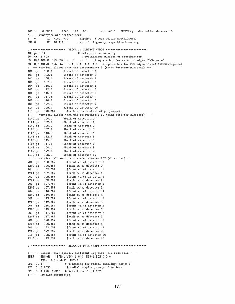
409 1 -0.9500 1209 -110 -30 imp:n=69.9 $HDPE cylinder behind detecor 10
c ---- graveyard and neutron beam ----
1 0 10 -100 -30 imp:n=1 $ void before spectrometer
999 0 30:-10:111 imp:n=0 $ graveyard/problem boundary
c ********************* BLOCK 2: SURFACE CARDS *************************
10 px -10 $ left problem boundary
30 CX 6.803 $ cylindrical surface of spectrometer
35 RPP 100.0 125.357 -1 1 -1 1 $ square box for detector edges (2x2square)
40 RPP 100.0 125.357 -1.1 1.1 -1.1 1.1 $ square box for PCB edges (1.1x1.100000.1square)
c --- vertical slices thru the spectrometer I (front detector surfaces) ---
100 px 100.0 $front of detector 0
101 px 102.5 $front of detector 1
102 px 105.0 $front of detector 2
103 px 107.5 $front of detector 3
104 px 110.0 $front of detector 4
105 px 112.5 $front of detector 5
106 px 115.0 $front of detector 6
107 px 117.5 $front of detector 7
108 px 120.0 $front of detector 8
109 px 122.5 $front of detector 9
110 px 125.0 $front of detector 10
111 px 125.357 $back of last sheet of poly/spectr
c --- vertical slices thru the spectrometer II (back detector surfaces) ---
1100 px 100.1 $back of detector 0
1101 px 102.6 $back of detector 1
1102 px 105.1 $back of detector 2
1103 px 107.6 $back of detector 3
1104 px 110.1 $back of detector 4
1105 px 112.6 $back of detector 5
1106 px 115.1 $back of detector 6
1107 px 117.6 $back of detector 7
1108 px 120.1 $back of detector 8
1109 px 122.6 $back of detector 9
1110 px 125.1 $back of detector 10
c --- vertical slices thru the spectrometer III (Cd slices) ---
200 px 100.257 $front cd of detector 0
1200 px 100.357 $back cd of detector 0
201 px 102.757 $front cd of detector 1
1201 px 102.857 $back cd of detector 1
202 px 105.257 $front cd of detector 2
1202 px 105.357 $back cd of detector 2
203 px 107.757 $front cd of detector 3
1203 px 107.857 $back cd of detector 3
204 px 110.257 $front cd of detector 4
1204 px 110.357 $back cd of detector 4
205 px 112.757 $front cd of detector 5
1205 px 112.857 $back cd of detector 5
206 px 115.257 $front cd of detector 6
1206 px 115.357 $back cd of detector 6
207 px 117.757 $front cd of detector 7
1207 px 117.857 $back cd of detector 7
208 px 120.257 $front cd of detector 8
1208 px 120.357 $back cd of detector 8
209 px 122.757 $front cd of detector 9
1209 px 122.857 $back cd of detector 9
210 px 125.257 $front cd of detector 10
1210 px 125.357 $back cd of detector 10
c ********************* BLOCK 3: DATA CARDS ****************************
c
c ----- Source: disk source, different erg dist. for each file ----
SDEF ERG=d1 PAR=1 VEC= 1 0 0 DIR=1 POS 0 0 0
AXS=1 0 0 rad=d2 EXT=0
SP2 -21 1 $ weighting for radial sampling: her r^1
SI2 0 6.8030 $ radial sampling range: 0 to Rmax
SP1 -3 1.025 2.926 $ Watt distn for f-252
c ----- Problem parameters
177
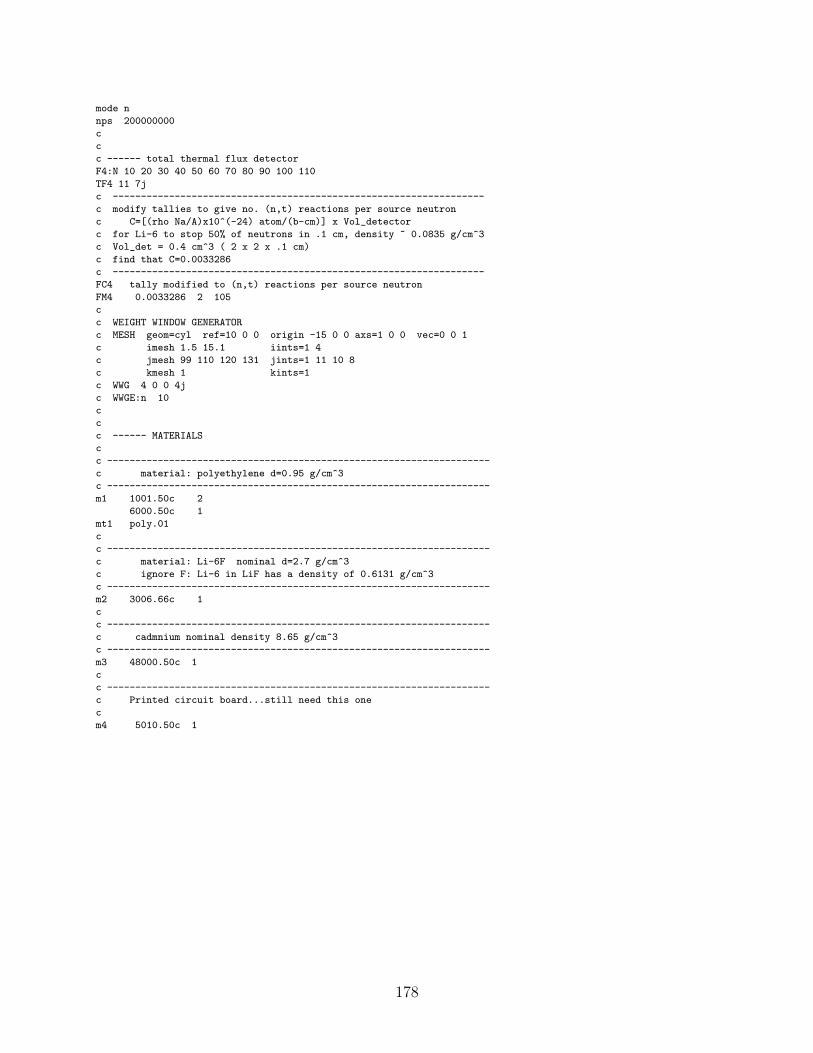
mode n
nps 200000000
c
c
c ------ total thermal flux detector
F4:N 10 20 30 40 50 60 70 80 90 100 110
TF4 11 7j
c ------------------------------------------------------------------
c modify tallies to give no. (n,t) reactions per source neutron
c C=[(rho Na/A)x10^(-24) atom/(b-cm)] x Vol_detector
c for Li-6 to stop 50% of neutrons in .1 cm, density ~ 0.0835 g/cm^3
c Vol_det = 0.4 cm^3 ( 2 x 2 x .1 cm)
c find that C=0.0033286
c ------------------------------------------------------------------
FC4 tally modified to (n,t) reactions per source neutron
FM4 0.0033286 2 105
c
c WEIGHT WINDOW GENERATOR
c MESH geom=cyl ref=10 0 0 origin -15 0 0 axs=1 0 0 vec=0 0 1
c imesh 1.5 15.1 iints=1 4
c jmesh 99 110 120 131 jints=1 11 10 8
c kmesh 1 kints=1
c WWG 4 0 0 4j
c WWGE:n 10
c
c
c ------ MATERIALS
c
c --------------------------------------------------------------------
c material: polyethylene d=0.95 g/cm^3
c --------------------------------------------------------------------
m1 1001.50c 2
6000.50c 1
mt1 poly.01
c
c --------------------------------------------------------------------
c material: Li-6F nominal d=2.7 g/cm^3
c ignore F: Li-6 in LiF has a density of 0.6131 g/cm^3
c --------------------------------------------------------------------
m2 3006.66c 1
c
c --------------------------------------------------------------------
c cadmnium nominal density 8.65 g/cm^3
c --------------------------------------------------------------------
m3 48000.50c 1
c
c --------------------------------------------------------------------
c Printed circuit board...still need this one
c
m4 5010.50c 1
178
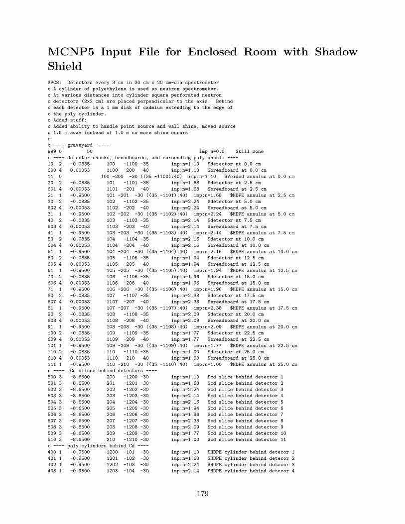
MCNP5 Input File for Enclosed Room with Shadow
ShieldSPC8: Detectors every 3 cm in 30 cm x 20 cm-dia spectrometer
c A cylinder of polyethylene is used as neutron spectrometer.
c At various distances into cylinder square perforated neutron
c detectors (2x2 cm) are placed perpendicular to the axis. Behind
c each detector is a 1 mm disk of cadmium extending to the edge of
c the poly cyclinder.
c Added stuff:
c Added ability to handle point source and wall shine, moved source
c 1.5 m away instead of 1.0 m so more shine occurs
c
c ---- graveyard ----
999 0 50 imp:n=0.0 $kill zone
c ---- detector chunks, breadboards, and surounding poly annuli ----
10 2 -0.0835 100 -1100 -35 imp:n=1.10 $detector at 0.0 cm
600 4 0.00053 1100 -200 -40 imp:n=1.10 $breadboard at 0.0 cm
11 0 100 -200 -30 ((35 -1100):40) imp:n=1.10 $Voided annulus at 0.0 cm
20 2 -0.0835 101 -1101 -35 imp:n=1.68 $detector at 2.5 cm
601 4 0.00053 1101 -201 -40 imp:n=1.68 $breadboard at 2.5 cm
21 1 -0.9500 101 -201 -30 ((35 -1101):40) imp:n=1.68 $HDPE annulus at 2.5 cm
30 2 -0.0835 102 -1102 -35 imp:n=2.24 $detector at 5.0 cm
602 4 0.00053 1102 -202 -40 imp:n=2.24 $breadboard at 5.0 cm
31 1 -0.9500 102 -202 -30 ((35 -1102):40) imp:n=2.24 $HDPE annulus at 5.0 cm
40 2 -0.0835 103 -1103 -35 imp:n=2.14 $detector at 7.5 cm
603 4 0.00053 1103 -203 -40 imp:n=2.14 $breadboard at 7.5 cm
41 1 -0.9500 103 -203 -30 ((35 -1103):40) imp:n=2.14 $HDPE annulus at 7.5 cm
50 2 -0.0835 104 -1104 -35 imp:n=2.16 $detector at 10.0 cm
604 4 0.00053 1104 -204 -40 imp:n=2.16 $breadboard at 10.0 cm
51 1 -0.9500 104 -204 -30 ((35 -1104):40) imp:n=2.16 $HDPE annulus at 10.0 cm
60 2 -0.0835 105 -1105 -35 imp:n=1.94 $detector at 12.5 cm
605 4 0.00053 1105 -205 -40 imp:n=1.94 $breadboard at 12.5 cm
61 1 -0.9500 105 -205 -30 ((35 -1105):40) imp:n=1.94 $HDPE annulus at 12.5 cm
70 2 -0.0835 106 -1106 -35 imp:n=1.96 $detector at 15.0 cm
606 4 0.00053 1106 -206 -40 imp:n=1.96 $breadboard at 15.0 cm
71 1 -0.9500 106 -206 -30 ((35 -1106):40) imp:n=1.96 $HDPE annulus at 15.0 cm
80 2 -0.0835 107 -1107 -35 imp:n=2.38 $detector at 17.5 cm
607 4 0.00053 1107 -207 -40 imp:n=2.38 $breadboard at 17.5 cm
81 1 -0.9500 107 -207 -30 ((35 -1107):40) imp:n=2.38 $HDPE annulus at 17.5 cm
90 2 -0.0835 108 -1108 -35 imp:n=2.09 $detector at 20.0 cm
608 4 0.00053 1108 -208 -40 imp:n=2.09 $breadboard at 20.0 cm
91 1 -0.9500 108 -208 -30 ((35 -1108):40) imp:n=2.09 $HDPE annulus at 20.0 cm
100 2 -0.0835 109 -1109 -35 imp:n=1.77 $detector at 22.5 cm
609 4 0.00053 1109 -209 -40 imp:n=1.77 $breadboard at 22.5 cm
101 1 -0.9500 109 -209 -30 ((35 -1109):40) imp:n=1.77 $HDPE annulus at 22.5 cm
110 2 -0.0835 110 -1110 -35 imp:n=1.00 $detector at 25.0 cm
610 4 0.00053 1110 -210 -40 imp:n=1.00 $breadboard at 25.0 cm
111 1 -0.9500 110 -210 -30 ((35 -1110):40) imp:n=1.00 $HDPE annulus at 25.0 cm
c ---- Cd slices behind detectors ----
500 3 -8.6500 200 -1200 -30 imp:n=1.10 $cd slice behind detector 1
501 3 -8.6500 201 -1201 -30 imp:n=1.68 $cd slice behind detector 2
502 3 -8.6500 202 -1202 -30 imp:n=2.24 $cd slice behind detector 3
503 3 -8.6500 203 -1203 -30 imp:n=2.14 $cd slice behind detector 4
504 3 -8.6500 204 -1204 -30 imp:n=2.16 $cd slice behind detector 5
505 3 -8.6500 205 -1205 -30 imp:n=1.94 $cd slice behind detector 6
506 3 -8.6500 206 -1206 -30 imp:n=1.96 $cd slice behind detector 7
507 3 -8.6500 207 -1207 -30 imp:n=2.38 $cd slice behind detector 8
508 3 -8.6500 208 -1208 -30 imp:n=2.09 $cd slice behind detector 9
509 3 -8.6500 209 -1209 -30 imp:n=1.77 $cd slice behind detector 10
510 3 -8.6500 210 -1210 -30 imp:n=1.00 $cd slice behind detector 11
c ---- poly cylinders behind Cd ----
400 1 -0.9500 1200 -101 -30 imp:n=1.10 $HDPE cylinder behind detecor 1
401 1 -0.9500 1201 -102 -30 imp:n=1.68 $HDPE cylinder behind detecor 2
402 1 -0.9500 1202 -103 -30 imp:n=2.24 $HDPE cylinder behind detecor 3
403 1 -0.9500 1203 -104 -30 imp:n=2.14 $HDPE cylinder behind detecor 4
179
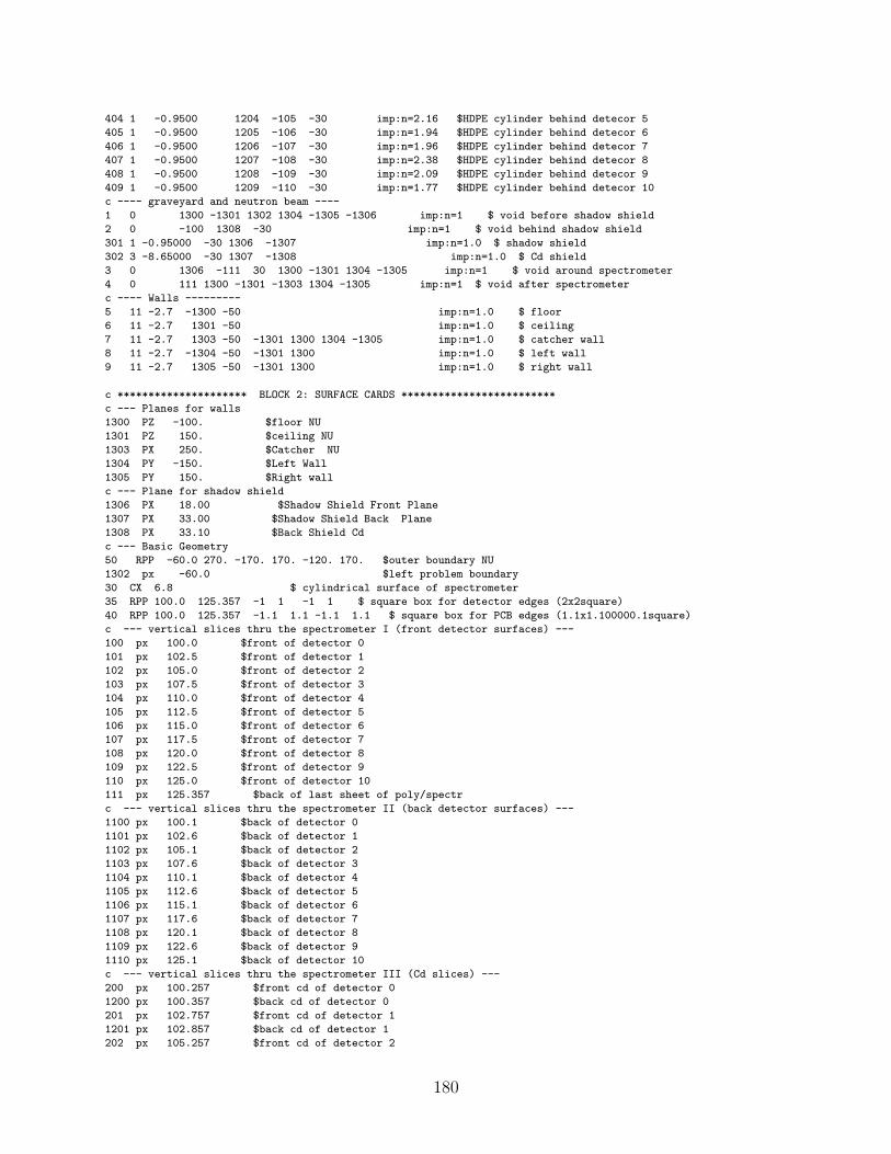
404 1 -0.9500 1204 -105 -30 imp:n=2.16 $HDPE cylinder behind detecor 5
405 1 -0.9500 1205 -106 -30 imp:n=1.94 $HDPE cylinder behind detecor 6
406 1 -0.9500 1206 -107 -30 imp:n=1.96 $HDPE cylinder behind detecor 7
407 1 -0.9500 1207 -108 -30 imp:n=2.38 $HDPE cylinder behind detecor 8
408 1 -0.9500 1208 -109 -30 imp:n=2.09 $HDPE cylinder behind detecor 9
409 1 -0.9500 1209 -110 -30 imp:n=1.77 $HDPE cylinder behind detecor 10
c ---- graveyard and neutron beam ----
1 0 1300 -1301 1302 1304 -1305 -1306 imp:n=1 $ void before shadow shield
2 0 -100 1308 -30 imp:n=1 $ void behind shadow shield
301 1 -0.95000 -30 1306 -1307 imp:n=1.0 $ shadow shield
302 3 -8.65000 -30 1307 -1308 imp:n=1.0 $ Cd shield
3 0 1306 -111 30 1300 -1301 1304 -1305 imp:n=1 $ void around spectrometer
4 0 111 1300 -1301 -1303 1304 -1305 imp:n=1 $ void after spectrometer
c ---- Walls ---------
5 11 -2.7 -1300 -50 imp:n=1.0 $ floor
6 11 -2.7 1301 -50 imp:n=1.0 $ ceiling
7 11 -2.7 1303 -50 -1301 1300 1304 -1305 imp:n=1.0 $ catcher wall
8 11 -2.7 -1304 -50 -1301 1300 imp:n=1.0 $ left wall
9 11 -2.7 1305 -50 -1301 1300 imp:n=1.0 $ right wall
c ********************* BLOCK 2: SURFACE CARDS *************************
c --- Planes for walls
1300 PZ -100. $floor NU
1301 PZ 150. $ceiling NU
1303 PX 250. $Catcher NU
1304 PY -150. $Left Wall
1305 PY 150. $Right wall
c --- Plane for shadow shield
1306 PX 18.00 $Shadow Shield Front Plane
1307 PX 33.00 $Shadow Shield Back Plane
1308 PX 33.10 $Back Shield Cd
c --- Basic Geometry
50 RPP -60.0 270. -170. 170. -120. 170. $outer boundary NU
1302 px -60.0 $left problem boundary
30 CX 6.8 $ cylindrical surface of spectrometer
35 RPP 100.0 125.357 -1 1 -1 1 $ square box for detector edges (2x2square)
40 RPP 100.0 125.357 -1.1 1.1 -1.1 1.1 $ square box for PCB edges (1.1x1.100000.1square)
c --- vertical slices thru the spectrometer I (front detector surfaces) ---
100 px 100.0 $front of detector 0
101 px 102.5 $front of detector 1
102 px 105.0 $front of detector 2
103 px 107.5 $front of detector 3
104 px 110.0 $front of detector 4
105 px 112.5 $front of detector 5
106 px 115.0 $front of detector 6
107 px 117.5 $front of detector 7
108 px 120.0 $front of detector 8
109 px 122.5 $front of detector 9
110 px 125.0 $front of detector 10
111 px 125.357 $back of last sheet of poly/spectr
c --- vertical slices thru the spectrometer II (back detector surfaces) ---
1100 px 100.1 $back of detector 0
1101 px 102.6 $back of detector 1
1102 px 105.1 $back of detector 2
1103 px 107.6 $back of detector 3
1104 px 110.1 $back of detector 4
1105 px 112.6 $back of detector 5
1106 px 115.1 $back of detector 6
1107 px 117.6 $back of detector 7
1108 px 120.1 $back of detector 8
1109 px 122.6 $back of detector 9
1110 px 125.1 $back of detector 10
c --- vertical slices thru the spectrometer III (Cd slices) ---
200 px 100.257 $front cd of detector 0
1200 px 100.357 $back cd of detector 0
201 px 102.757 $front cd of detector 1
1201 px 102.857 $back cd of detector 1
202 px 105.257 $front cd of detector 2
180
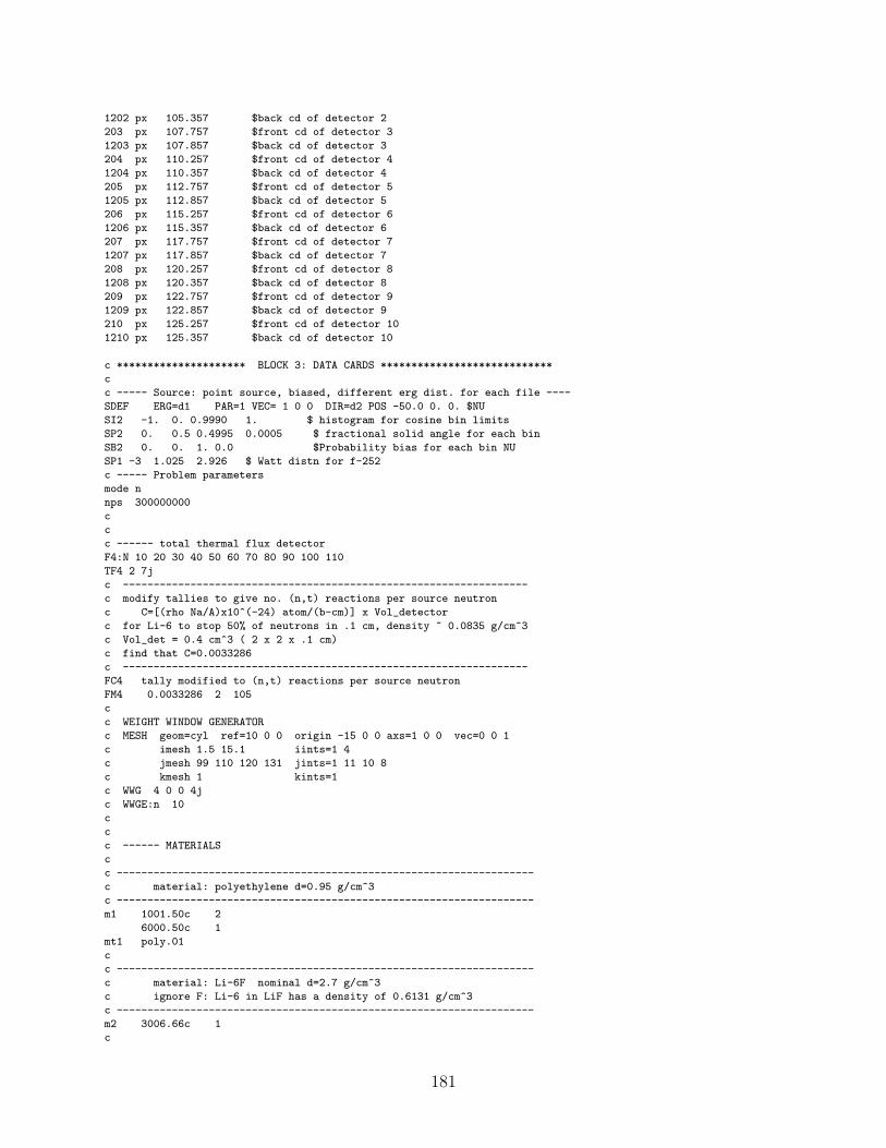
1202 px 105.357 $back cd of detector 2
203 px 107.757 $front cd of detector 3
1203 px 107.857 $back cd of detector 3
204 px 110.257 $front cd of detector 4
1204 px 110.357 $back cd of detector 4
205 px 112.757 $front cd of detector 5
1205 px 112.857 $back cd of detector 5
206 px 115.257 $front cd of detector 6
1206 px 115.357 $back cd of detector 6
207 px 117.757 $front cd of detector 7
1207 px 117.857 $back cd of detector 7
208 px 120.257 $front cd of detector 8
1208 px 120.357 $back cd of detector 8
209 px 122.757 $front cd of detector 9
1209 px 122.857 $back cd of detector 9
210 px 125.257 $front cd of detector 10
1210 px 125.357 $back cd of detector 10
c ********************* BLOCK 3: DATA CARDS ****************************
c
c ----- Source: point source, biased, different erg dist. for each file ----
SDEF ERG=d1 PAR=1 VEC= 1 0 0 DIR=d2 POS -50.0 0. 0. $NU
SI2 -1. 0. 0.9990 1. $ histogram for cosine bin limits
SP2 0. 0.5 0.4995 0.0005 $ fractional solid angle for each bin
SB2 0. 0. 1. 0.0 $Probability bias for each bin NU
SP1 -3 1.025 2.926 $ Watt distn for f-252
c ----- Problem parameters
mode n
nps 300000000
c
c
c ------ total thermal flux detector
F4:N 10 20 30 40 50 60 70 80 90 100 110
TF4 2 7j
c ------------------------------------------------------------------
c modify tallies to give no. (n,t) reactions per source neutron
c C=[(rho Na/A)x10^(-24) atom/(b-cm)] x Vol_detector
c for Li-6 to stop 50% of neutrons in .1 cm, density ~ 0.0835 g/cm^3
c Vol_det = 0.4 cm^3 ( 2 x 2 x .1 cm)
c find that C=0.0033286
c ------------------------------------------------------------------
FC4 tally modified to (n,t) reactions per source neutron
FM4 0.0033286 2 105
c
c WEIGHT WINDOW GENERATOR
c MESH geom=cyl ref=10 0 0 origin -15 0 0 axs=1 0 0 vec=0 0 1
c imesh 1.5 15.1 iints=1 4
c jmesh 99 110 120 131 jints=1 11 10 8
c kmesh 1 kints=1
c WWG 4 0 0 4j
c WWGE:n 10
c
c
c ------ MATERIALS
c
c --------------------------------------------------------------------
c material: polyethylene d=0.95 g/cm^3
c --------------------------------------------------------------------
m1 1001.50c 2
6000.50c 1
mt1 poly.01
c
c --------------------------------------------------------------------
c material: Li-6F nominal d=2.7 g/cm^3
c ignore F: Li-6 in LiF has a density of 0.6131 g/cm^3
c --------------------------------------------------------------------
m2 3006.66c 1
c
181
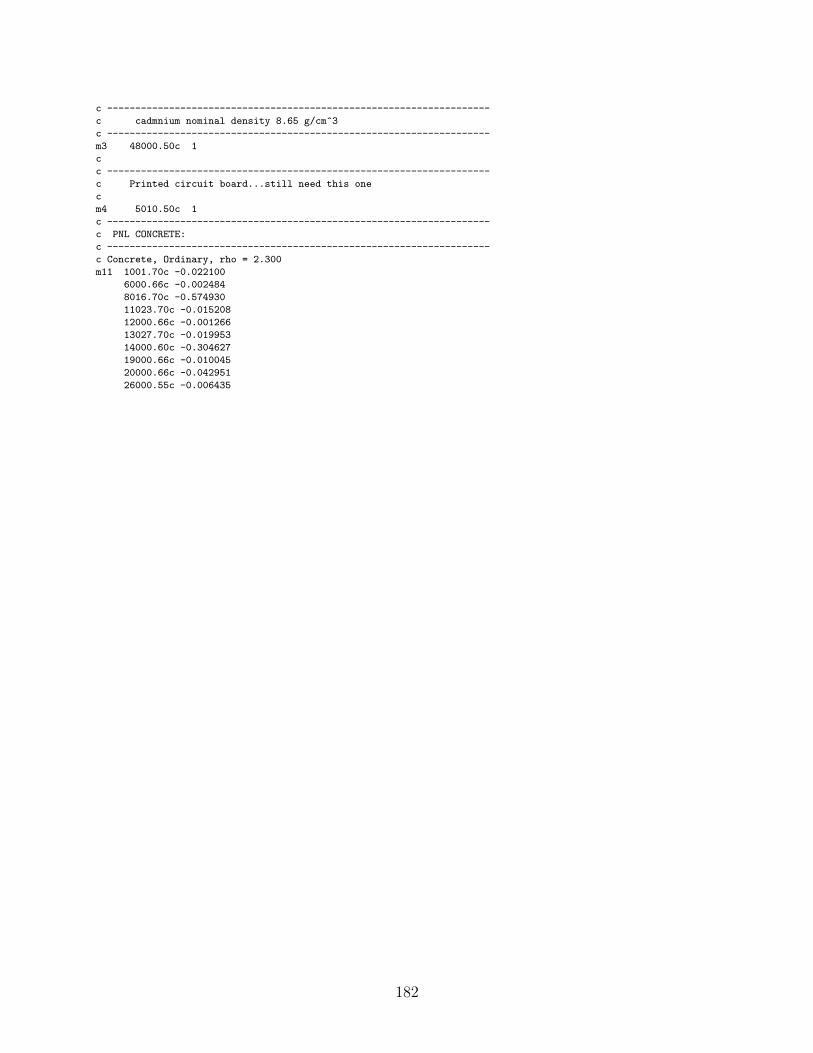
c --------------------------------------------------------------------
c cadmnium nominal density 8.65 g/cm^3
c --------------------------------------------------------------------
m3 48000.50c 1
c
c --------------------------------------------------------------------
c Printed circuit board...still need this one
c
m4 5010.50c 1
c --------------------------------------------------------------------
c PNL CONCRETE:
c --------------------------------------------------------------------
c Concrete, Ordinary, rho = 2.300
m11 1001.70c -0.022100
6000.66c -0.002484
8016.70c -0.574930
11023.70c -0.015208
12000.66c -0.001266
13027.70c -0.019953
14000.60c -0.304627
19000.66c -0.010045
20000.66c -0.042951
26000.55c -0.006435
182
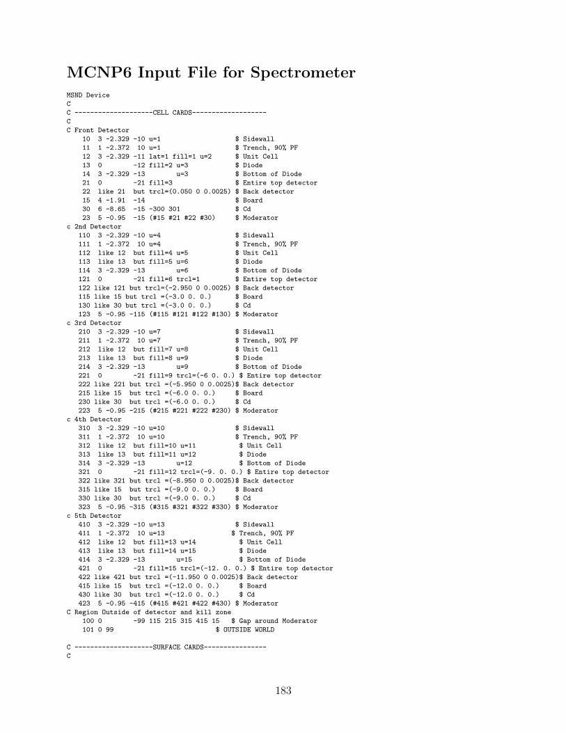
MCNP6 Input File for SpectrometerMSND Device
C
C --------------------CELL CARDS-------------------
C
C Front Detector
10 3 -2.329 -10 u=1 $ Sidewall
11 1 -2.372 10 u=1 $ Trench, 90% PF
12 3 -2.329 -11 lat=1 fill=1 u=2 $ Unit Cell
13 0 -12 fill=2 u=3 $ Diode
14 3 -2.329 -13 u=3 $ Bottom of Diode
21 0 -21 fill=3 $ Entire top detector
22 like 21 but trcl=(0.050 0 0.0025) $ Back detector
15 4 -1.91 -14 $ Board
30 6 -8.65 -15 -300 301 $ Cd
23 5 -0.95 -15 (#15 #21 #22 #30) $ Moderator
c 2nd Detector
110 3 -2.329 -10 u=4 $ Sidewall
111 1 -2.372 10 u=4 $ Trench, 90% PF
112 like 12 but fill=4 u=5 $ Unit Cell
113 like 13 but fill=5 u=6 $ Diode
114 3 -2.329 -13 u=6 $ Bottom of Diode
121 0 -21 fill=6 trcl=1 $ Entire top detector
122 like 121 but trcl=(-2.950 0 0.0025) $ Back detector
115 like 15 but trcl =(-3.0 0. 0.) $ Board
130 like 30 but trcl =(-3.0 0. 0.) $ Cd
123 5 -0.95 -115 (#115 #121 #122 #130) $ Moderator
c 3rd Detector
210 3 -2.329 -10 u=7 $ Sidewall
211 1 -2.372 10 u=7 $ Trench, 90% PF
212 like 12 but fill=7 u=8 $ Unit Cell
213 like 13 but fill=8 u=9 $ Diode
214 3 -2.329 -13 u=9 $ Bottom of Diode
221 0 -21 fill=9 trcl=(-6 0. 0.) $ Entire top detector
222 like 221 but trcl =(-5.950 0 0.0025)$ Back detector
215 like 15 but trcl =(-6.0 0. 0.) $ Board
230 like 30 but trcl =(-6.0 0. 0.) $ Cd
223 5 -0.95 -215 (#215 #221 #222 #230) $ Moderator
c 4th Detector
310 3 -2.329 -10 u=10 $ Sidewall
311 1 -2.372 10 u=10 $ Trench, 90% PF
312 like 12 but fill=10 u=11 $ Unit Cell
313 like 13 but fill=11 u=12 $ Diode
314 3 -2.329 -13 u=12 $ Bottom of Diode
321 0 -21 fill=12 trcl=(-9. 0. 0.) $ Entire top detector
322 like 321 but trcl =(-8.950 0 0.0025)$ Back detector
315 like 15 but trcl =(-9.0 0. 0.) $ Board
330 like 30 but trcl =(-9.0 0. 0.) $ Cd
323 5 -0.95 -315 (#315 #321 #322 #330) $ Moderator
c 5th Detector
410 3 -2.329 -10 u=13 $ Sidewall
411 1 -2.372 10 u=13 $ Trench, 90% PF
412 like 12 but fill=13 u=14 $ Unit Cell
413 like 13 but fill=14 u=15 $ Diode
414 3 -2.329 -13 u=15 $ Bottom of Diode
421 0 -21 fill=15 trcl=(-12. 0. 0.) $ Entire top detector
422 like 421 but trcl =(-11.950 0 0.0025)$ Back detector
415 like 15 but trcl =(-12.0 0. 0.) $ Board
430 like 30 but trcl =(-12.0 0. 0.) $ Cd
423 5 -0.95 -415 (#415 #421 #422 #430) $ Moderator
C Region Outside of detector and kill zone
100 0 -99 115 215 315 415 15 $ Gap around Moderator
101 0 99 $ OUTSIDE WORLD
C --------------------SURFACE CARDS----------------
C
183
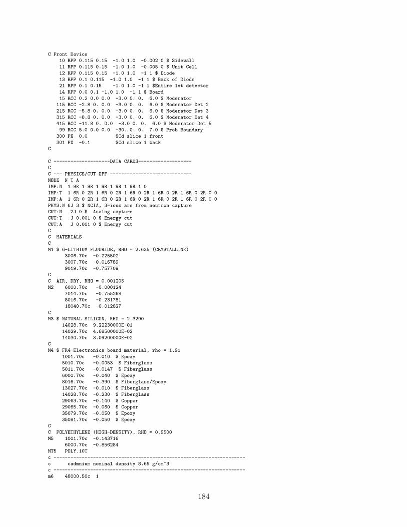
C Front Device
10 RPP 0.115 0.15 -1.0 1.0 -0.002 0 $ Sidewall
11 RPP 0.115 0.15 -1.0 1.0 -0.005 0 $ Unit Cell
12 RPP 0.115 0.15 -1.0 1.0 -1 1 $ Diode
13 RPP 0.1 0.115 -1.0 1.0 -1 1 $ Back of Diode
21 RPP 0.1 0.15 -1.0 1.0 -1 1 $Entire 1st detector
14 RPP 0.0 0.1 -1.0 1.0 -1 1 $ Board
15 RCC 0.2 0.0 0.0 -3.0 0. 0. 6.0 $ Moderator
115 RCC -2.8 0. 0.0 -3.0 0. 0. 6.0 $ Moderator Det 2
215 RCC -5.8 0. 0.0 -3.0 0. 0. 6.0 $ Moderator Det 3
315 RCC -8.8 0. 0.0 -3.0 0. 0. 6.0 $ Moderator Det 4
415 RCC -11.8 0. 0.0 -3.0 0. 0. 6.0 $ Moderator Det 5
99 RCC 5.0 0.0 0.0 -30. 0. 0. 7.0 $ Prob Boundary
300 PX 0.0 $Cd slice 1 front
301 PX -0.1 $Cd slice 1 back
C
C --------------------DATA CARDS-------------------
C
C --- PHYSICS/CUT OFF -----------------------------
MODE N T A
IMP:N 1 9R 1 9R 1 9R 1 9R 1 9R 1 0
IMP:T 1 6R 0 2R 1 6R 0 2R 1 6R 0 2R 1 6R 0 2R 1 6R 0 2R 0 0
IMP:A 1 6R 0 2R 1 6R 0 2R 1 6R 0 2R 1 6R 0 2R 1 6R 0 2R 0 0
PHYS:N 6J 3 $ NCIA, 3=ions are from neutron capture
CUT:N 2J 0 $ Analog capture
CUT:T J 0.001 0 $ Energy cut
CUT:A J 0.001 0 $ Energy cut
C
C MATERIALS
C
M1 $ 6-LITHIUM FLUORIDE, RHO = 2.635 (CRYSTALLINE)
3006.70c -0.225502
3007.70c -0.016789
9019.70c -0.757709
C
C AIR, DRY, RHO = 0.001205
M2 6000.70c -0.000124
7014.70c -0.755268
8016.70c -0.231781
18040.70c -0.012827
C
M3 $ NATURAL SILICON, RHO = 2.3290
14028.70c 9.22230000E-01
14029.70c 4.68500000E-02
14030.70c 3.09200000E-02
C
M4 $ FR4 Electronics board material, rho = 1.91
1001.70c -0.010 $ Epoxy
5010.70c -0.0053 $ Fiberglass
5011.70c -0.0147 $ Fiberglass
6000.70c -0.040 $ Epoxy
8016.70c -0.390 $ Fiberglass/Epoxy
13027.70c -0.010 $ Fiberglass
14028.70c -0.230 $ Fiberglass
29063.70c -0.140 $ Copper
29065.70c -0.060 $ Copper
35079.70c -0.050 $ Epoxy
35081.70c -0.050 $ Epoxy
C
C POLYETHYLENE (HIGH-DENSITY), RHO = 0.9500
M5 1001.70c -0.143716
6000.70c -0.856284
MT5 POLY.10T
c --------------------------------------------------------------------
c cadmnium nominal density 8.65 g/cm^3
c --------------------------------------------------------------------
m6 48000.50c 1
184
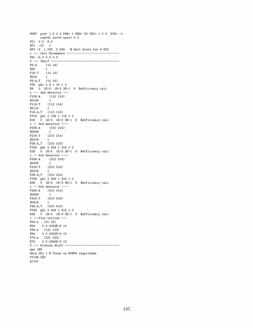
SDEF pos= 1.5 0 0 PAR= 1 ERG= D2 VEC= 1 0 0 DIR= -1.
rad=d1 ext=0 axs=1 0 0
SI1 0.0 6.0
SP1 -21 1
SP2 -3 1.025 2.926 $ Watt distn for f-252
c --- Cell Movements ------------------------------
TR1 -3.0 0.0 0.0
C --- TALLY ---------------------------------------
F6:A (10 14)
SD6 1
F16:T (10 14)
SD16 1
F8:A,T (10 14)
FT8 phl 2 6 1 16 1 0
E8 0 1E-5 1E-3 3E-1 5 $efficiency calc
c --- 2nd detector ---
F106:A (110 114)
SD106 1
F116:T (110 114)
SD116 1
F18:A,T (110 114)
FT18 phl 2 106 1 116 1 0
E18 0 1E-5 1E-3 3E-1 5 $efficiency calc
c -- 3rd detector ----
F206:A (210 214)
SD206 1
F216:T (210 214)
SD216 1
F28:A,T (210 214)
FT28 phl 2 206 1 216 1 0
E28 0 1E-5 1E-3 3E-1 5 $efficiency calc
c -- 4th detector ----
F306:A (310 314)
SD306 1
F316:T (310 314)
SD316 1
F38:A,T (310 314)
FT38 phl 2 306 1 316 1 0
E38 0 1E-5 1E-3 3E-1 5 $efficiency calc
c -- 5th detector ----
F406:A (410 414)
SD406 1
F416:T (410 414)
SD416 1
F48:A,T (410 414)
FT48 phl 2 406 1 416 1 0
E48 0 1E-5 1E-3 3E-1 5 $efficiency calc
c ---flux tallies ---
F54:n (21 22)
E54 0 0.0254E-6 10
F64:n (121 122)
E64 0 0.0254E-6 10
F74:n (221 222)
E74 0 0.0254E-6 10
C --- Problem Stuff -------------------------------
nps 1E8
dbcn 28j 1 $ Turns on MCNPX algorithms
FT138 CAP
185
Appendix D
Example Tabulated Data forSpectrometer Simulations
Description Starting Page
Example of simulation data for a neutron beamuniformly irradiating a spectrometer in a void forvarious values of t.
187
Example of simulated counting measurements forroom scatter and void template simulations fora point source with concrete floor. The opti-mal shadow shield and several sources were used.The spectrometer has the geometric parametersNdet = 11, r =6.8 cm, t = 2.5 cm.
193
186
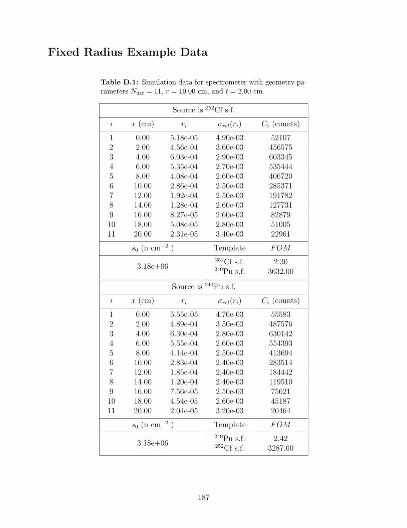
Fixed Radius Example Data
Table D.1: Simulation data for spectrometer with geometry pa-rameters Ndet = 11, r = 10.00 cm, and t = 2.00 cm.
Source is 252Cf s.f.
i x (cm) ri σrel(ri) Ci (counts)
1 0.00 5.18e-05 4.90e-03 521072 2.00 4.56e-04 3.60e-03 4565753 4.00 6.03e-04 2.90e-03 6033454 6.00 5.35e-04 2.70e-03 5354445 8.00 4.08e-04 2.60e-03 4067206 10.00 2.86e-04 2.50e-03 2853717 12.00 1.92e-04 2.50e-03 1917828 14.00 1.28e-04 2.60e-03 1277319 16.00 8.27e-05 2.60e-03 8287910 18.00 5.08e-05 2.80e-03 5100511 20.00 2.31e-05 3.40e-03 22961
s0 (n cm−2 ) Template FOM
3.18e+06252Cf s.f. 2.30240Pu s.f. 3632.00
Source is 240Pu s.f.
i x (cm) ri σrel(ri) Ci (counts)
1 0.00 5.55e-05 4.70e-03 555832 2.00 4.89e-04 3.50e-03 4875763 4.00 6.30e-04 2.80e-03 6301424 6.00 5.55e-04 2.60e-03 5543935 8.00 4.14e-04 2.50e-03 4136946 10.00 2.83e-04 2.40e-03 2835147 12.00 1.85e-04 2.40e-03 1844428 14.00 1.20e-04 2.40e-03 1195109 16.00 7.56e-05 2.50e-03 7562110 18.00 4.54e-05 2.60e-03 4518711 20.00 2.04e-05 3.20e-03 20464
s0 (n cm−2 ) Template FOM
3.18e+06240Pu s.f. 2.42252Cf s.f. 3287.00
187
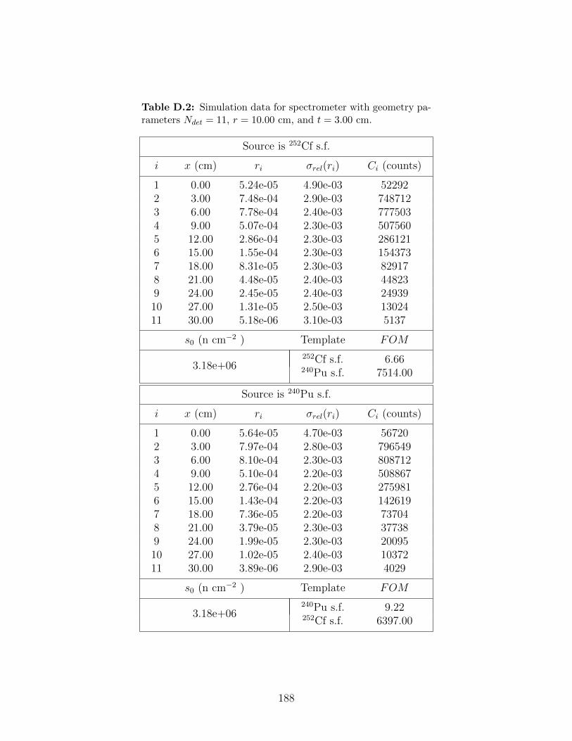
Table D.2: Simulation data for spectrometer with geometry pa-rameters Ndet = 11, r = 10.00 cm, and t = 3.00 cm.
Source is 252Cf s.f.
i x (cm) ri σrel(ri) Ci (counts)
1 0.00 5.24e-05 4.90e-03 522922 3.00 7.48e-04 2.90e-03 7487123 6.00 7.78e-04 2.40e-03 7775034 9.00 5.07e-04 2.30e-03 5075605 12.00 2.86e-04 2.30e-03 2861216 15.00 1.55e-04 2.30e-03 1543737 18.00 8.31e-05 2.30e-03 829178 21.00 4.48e-05 2.40e-03 448239 24.00 2.45e-05 2.40e-03 2493910 27.00 1.31e-05 2.50e-03 1302411 30.00 5.18e-06 3.10e-03 5137
s0 (n cm−2 ) Template FOM
3.18e+06252Cf s.f. 6.66240Pu s.f. 7514.00
Source is 240Pu s.f.
i x (cm) ri σrel(ri) Ci (counts)
1 0.00 5.64e-05 4.70e-03 567202 3.00 7.97e-04 2.80e-03 7965493 6.00 8.10e-04 2.30e-03 8087124 9.00 5.10e-04 2.20e-03 5088675 12.00 2.76e-04 2.20e-03 2759816 15.00 1.43e-04 2.20e-03 1426197 18.00 7.36e-05 2.20e-03 737048 21.00 3.79e-05 2.30e-03 377389 24.00 1.99e-05 2.30e-03 2009510 27.00 1.02e-05 2.40e-03 1037211 30.00 3.89e-06 2.90e-03 4029
s0 (n cm−2 ) Template FOM
3.18e+06240Pu s.f. 9.22252Cf s.f. 6397.00
188
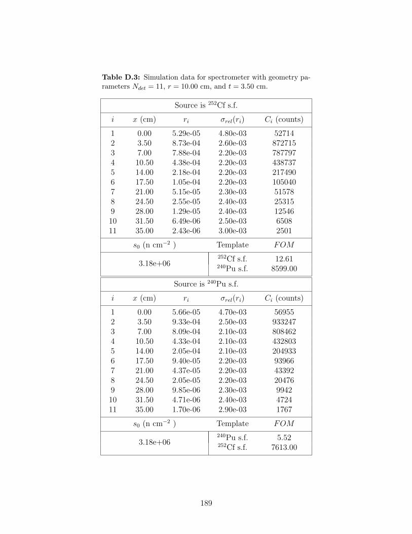
Table D.3: Simulation data for spectrometer with geometry pa-rameters Ndet = 11, r = 10.00 cm, and t = 3.50 cm.
Source is 252Cf s.f.
i x (cm) ri σrel(ri) Ci (counts)
1 0.00 5.29e-05 4.80e-03 527142 3.50 8.73e-04 2.60e-03 8727153 7.00 7.88e-04 2.20e-03 7877974 10.50 4.38e-04 2.20e-03 4387375 14.00 2.18e-04 2.20e-03 2174906 17.50 1.05e-04 2.20e-03 1050407 21.00 5.15e-05 2.30e-03 515788 24.50 2.55e-05 2.40e-03 253159 28.00 1.29e-05 2.40e-03 1254610 31.50 6.49e-06 2.50e-03 650811 35.00 2.43e-06 3.00e-03 2501
s0 (n cm−2 ) Template FOM
3.18e+06252Cf s.f. 12.61240Pu s.f. 8599.00
Source is 240Pu s.f.
i x (cm) ri σrel(ri) Ci (counts)
1 0.00 5.66e-05 4.70e-03 569552 3.50 9.33e-04 2.50e-03 9332473 7.00 8.09e-04 2.10e-03 8084624 10.50 4.33e-04 2.10e-03 4328035 14.00 2.05e-04 2.10e-03 2049336 17.50 9.40e-05 2.20e-03 939667 21.00 4.37e-05 2.20e-03 433928 24.50 2.05e-05 2.20e-03 204769 28.00 9.85e-06 2.30e-03 994210 31.50 4.71e-06 2.40e-03 472411 35.00 1.70e-06 2.90e-03 1767
s0 (n cm−2 ) Template FOM
3.18e+06240Pu s.f. 5.52252Cf s.f. 7613.00
189
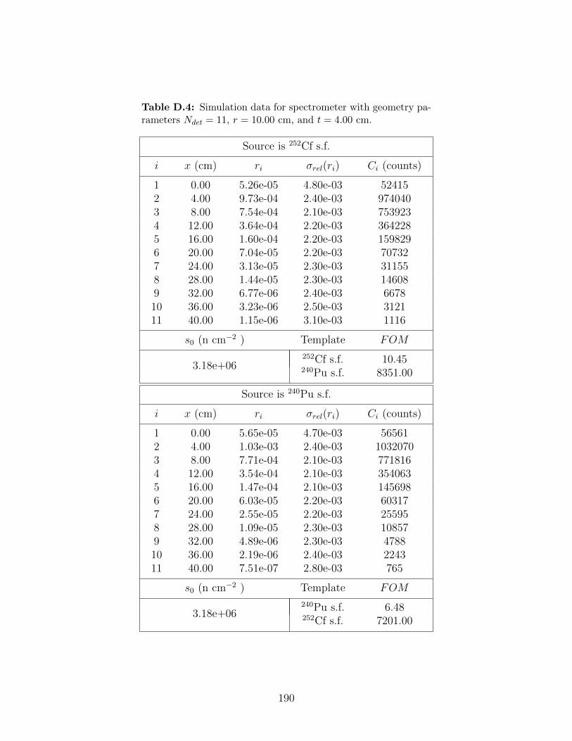
Table D.4: Simulation data for spectrometer with geometry pa-rameters Ndet = 11, r = 10.00 cm, and t = 4.00 cm.
Source is 252Cf s.f.
i x (cm) ri σrel(ri) Ci (counts)
1 0.00 5.26e-05 4.80e-03 524152 4.00 9.73e-04 2.40e-03 9740403 8.00 7.54e-04 2.10e-03 7539234 12.00 3.64e-04 2.20e-03 3642285 16.00 1.60e-04 2.20e-03 1598296 20.00 7.04e-05 2.20e-03 707327 24.00 3.13e-05 2.30e-03 311558 28.00 1.44e-05 2.30e-03 146089 32.00 6.77e-06 2.40e-03 667810 36.00 3.23e-06 2.50e-03 312111 40.00 1.15e-06 3.10e-03 1116
s0 (n cm−2 ) Template FOM
3.18e+06252Cf s.f. 10.45240Pu s.f. 8351.00
Source is 240Pu s.f.
i x (cm) ri σrel(ri) Ci (counts)
1 0.00 5.65e-05 4.70e-03 565612 4.00 1.03e-03 2.40e-03 10320703 8.00 7.71e-04 2.10e-03 7718164 12.00 3.54e-04 2.10e-03 3540635 16.00 1.47e-04 2.10e-03 1456986 20.00 6.03e-05 2.20e-03 603177 24.00 2.55e-05 2.20e-03 255958 28.00 1.09e-05 2.30e-03 108579 32.00 4.89e-06 2.30e-03 478810 36.00 2.19e-06 2.40e-03 224311 40.00 7.51e-07 2.80e-03 765
s0 (n cm−2 ) Template FOM
3.18e+06240Pu s.f. 6.48252Cf s.f. 7201.00
190
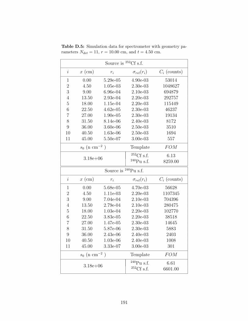
Table D.5: Simulation data for spectrometer with geometry pa-rameters Ndet = 11, r = 10.00 cm, and t = 4.50 cm.
Source is 252Cf s.f.
i x (cm) ri σrel(ri) Ci (counts)
1 0.00 5.29e-05 4.90e-03 530142 4.50 1.05e-03 2.30e-03 10486273 9.00 6.96e-04 2.10e-03 6948794 13.50 2.93e-04 2.20e-03 2927575 18.00 1.15e-04 2.20e-03 1154496 22.50 4.62e-05 2.30e-03 462377 27.00 1.90e-05 2.30e-03 191348 31.50 8.14e-06 2.40e-03 81729 36.00 3.60e-06 2.50e-03 351010 40.50 1.63e-06 2.50e-03 169411 45.00 5.50e-07 3.00e-03 557
s0 (n cm−2 ) Template FOM
3.18e+06252Cf s.f. 6.13240Pu s.f. 8259.00
Source is 240Pu s.f.
i x (cm) ri σrel(ri) Ci (counts)
1 0.00 5.68e-05 4.70e-03 566282 4.50 1.11e-03 2.20e-03 11073453 9.00 7.04e-04 2.10e-03 7043964 13.50 2.79e-04 2.10e-03 2804755 18.00 1.03e-04 2.20e-03 1027706 22.50 3.83e-05 2.20e-03 385187 27.00 1.47e-05 2.30e-03 146458 31.50 5.87e-06 2.30e-03 58839 36.00 2.43e-06 2.40e-03 240310 40.50 1.03e-06 2.40e-03 100811 45.00 3.33e-07 3.00e-03 301
s0 (n cm−2 ) Template FOM
3.18e+06240Pu s.f. 6.61252Cf s.f. 6601.00
191
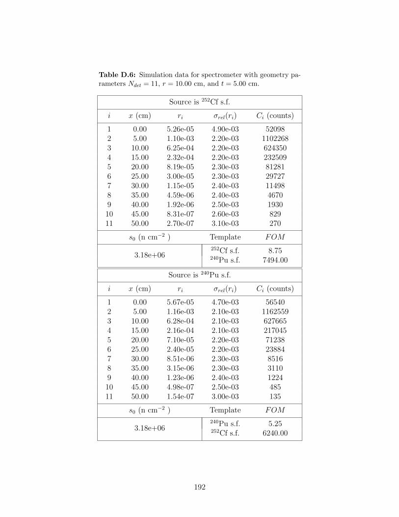
Table D.6: Simulation data for spectrometer with geometry pa-rameters Ndet = 11, r = 10.00 cm, and t = 5.00 cm.
Source is 252Cf s.f.
i x (cm) ri σrel(ri) Ci (counts)
1 0.00 5.26e-05 4.90e-03 520982 5.00 1.10e-03 2.20e-03 11022683 10.00 6.25e-04 2.20e-03 6243504 15.00 2.32e-04 2.20e-03 2325095 20.00 8.19e-05 2.30e-03 812816 25.00 3.00e-05 2.30e-03 297277 30.00 1.15e-05 2.40e-03 114988 35.00 4.59e-06 2.40e-03 46709 40.00 1.92e-06 2.50e-03 193010 45.00 8.31e-07 2.60e-03 82911 50.00 2.70e-07 3.10e-03 270
s0 (n cm−2 ) Template FOM
3.18e+06252Cf s.f. 8.75240Pu s.f. 7494.00
Source is 240Pu s.f.
i x (cm) ri σrel(ri) Ci (counts)
1 0.00 5.67e-05 4.70e-03 565402 5.00 1.16e-03 2.10e-03 11625593 10.00 6.28e-04 2.10e-03 6276654 15.00 2.16e-04 2.10e-03 2170455 20.00 7.10e-05 2.20e-03 712386 25.00 2.40e-05 2.20e-03 238847 30.00 8.51e-06 2.30e-03 85168 35.00 3.15e-06 2.30e-03 31109 40.00 1.23e-06 2.40e-03 122410 45.00 4.98e-07 2.50e-03 48511 50.00 1.54e-07 3.00e-03 135
s0 (n cm−2 ) Template FOM
3.18e+06240Pu s.f. 5.25252Cf s.f. 6240.00
192
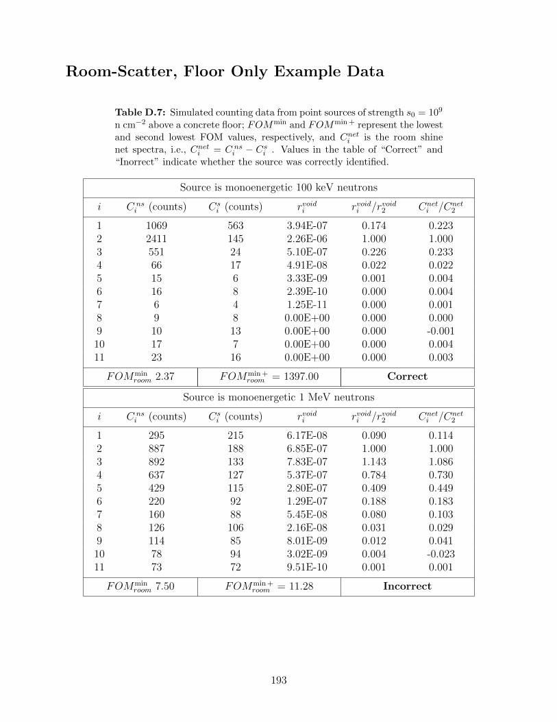
Room-Scatter, Floor Only Example Data
Table D.7: Simulated counting data from point sources of strength s0 = 109
n cm−2 above a concrete floor; FOMmin and FOMmin + represent the lowestand second lowest FOM values, respectively, and Cneti is the room shinenet spectra, i.e., Cneti = C ns
i − Csi . Values in the table of “Correct” and“Inorrect” indicate whether the source was correctly identified.
Source is monoenergetic 100 keV neutrons
i C nsi (counts) Cs
i (counts) rvoidi rvoidi /rvoid2 Cneti /Cnet
2
1 1069 563 3.94E-07 0.174 0.2232 2411 145 2.26E-06 1.000 1.0003 551 24 5.10E-07 0.226 0.2334 66 17 4.91E-08 0.022 0.0225 15 6 3.33E-09 0.001 0.0046 16 8 2.39E-10 0.000 0.0047 6 4 1.25E-11 0.000 0.0018 9 8 0.00E+00 0.000 0.0009 10 13 0.00E+00 0.000 -0.00110 17 7 0.00E+00 0.000 0.00411 23 16 0.00E+00 0.000 0.003
FOMminroom 2.37 FOMmin +
room = 1397.00 Correct
Source is monoenergetic 1 MeV neutrons
i C nsi (counts) Cs
i (counts) rvoidi rvoidi /rvoid2 Cneti /Cnet
2
1 295 215 6.17E-08 0.090 0.1142 887 188 6.85E-07 1.000 1.0003 892 133 7.83E-07 1.143 1.0864 637 127 5.37E-07 0.784 0.7305 429 115 2.80E-07 0.409 0.4496 220 92 1.29E-07 0.188 0.1837 160 88 5.45E-08 0.080 0.1038 126 106 2.16E-08 0.031 0.0299 114 85 8.01E-09 0.012 0.04110 78 94 3.02E-09 0.004 -0.02311 73 72 9.51E-10 0.001 0.001
FOMminroom 7.50 FOMmin +
room = 11.28 Incorrect
193
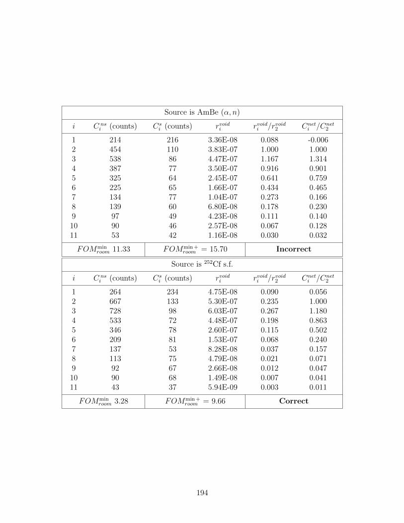
Source is AmBe (α, n)
i C nsi (counts) Cs
i (counts) rvoidi rvoidi /rvoid2 Cneti /Cnet
2
1 214 216 3.36E-08 0.088 -0.0062 454 110 3.83E-07 1.000 1.0003 538 86 4.47E-07 1.167 1.3144 387 77 3.50E-07 0.916 0.9015 325 64 2.45E-07 0.641 0.7596 225 65 1.66E-07 0.434 0.4657 134 77 1.04E-07 0.273 0.1668 139 60 6.80E-08 0.178 0.2309 97 49 4.23E-08 0.111 0.14010 90 46 2.57E-08 0.067 0.12811 53 42 1.16E-08 0.030 0.032
FOMminroom 11.33 FOMmin +
room = 15.70 Incorrect
Source is 252Cf s.f.
i C nsi (counts) Cs
i (counts) rvoidi rvoidi /rvoid2 Cneti /Cnet
2
1 264 234 4.75E-08 0.090 0.0562 667 133 5.30E-07 0.235 1.0003 728 98 6.03E-07 0.267 1.1804 533 72 4.48E-07 0.198 0.8635 346 78 2.60E-07 0.115 0.5026 209 81 1.53E-07 0.068 0.2407 137 53 8.28E-08 0.037 0.1578 113 75 4.79E-08 0.021 0.0719 92 67 2.66E-08 0.012 0.04710 90 68 1.49E-08 0.007 0.04111 43 37 5.94E-09 0.003 0.011
FOMminroom 3.28 FOMmin +
room = 9.66 Correct
194
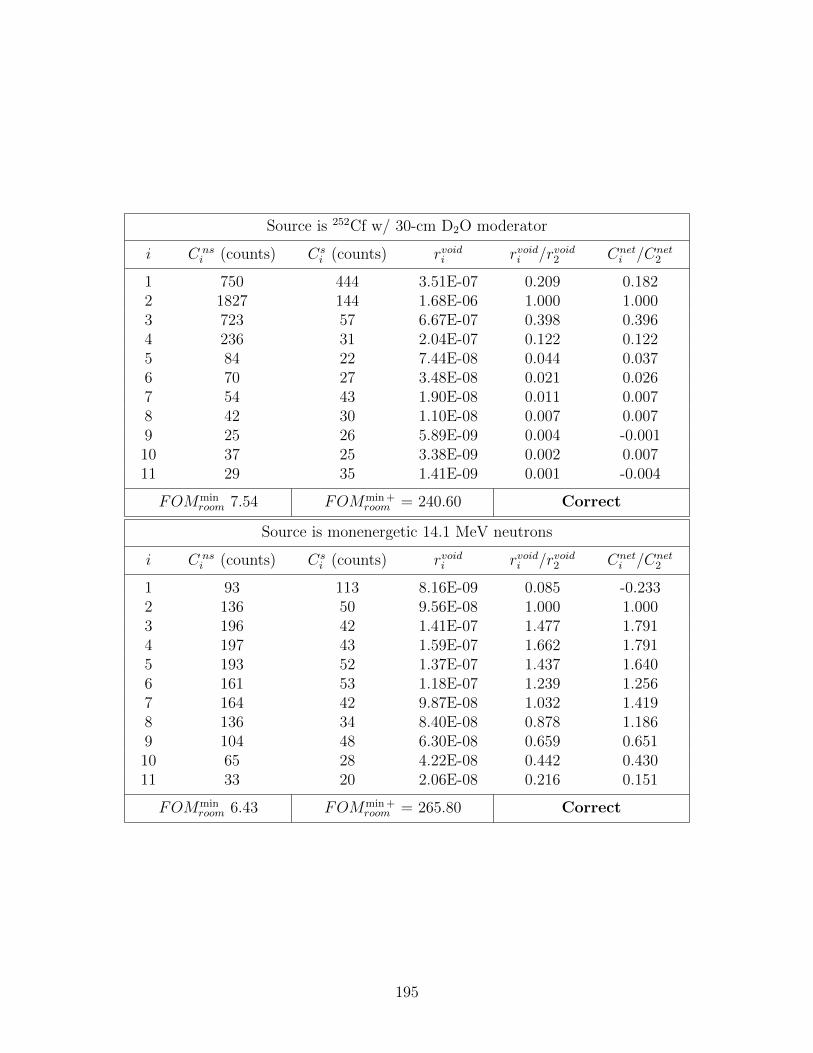
Source is 252Cf w/ 30-cm D2O moderator
i C nsi (counts) Cs
i (counts) rvoidi rvoidi /rvoid2 Cneti /Cnet
2
1 750 444 3.51E-07 0.209 0.1822 1827 144 1.68E-06 1.000 1.0003 723 57 6.67E-07 0.398 0.3964 236 31 2.04E-07 0.122 0.1225 84 22 7.44E-08 0.044 0.0376 70 27 3.48E-08 0.021 0.0267 54 43 1.90E-08 0.011 0.0078 42 30 1.10E-08 0.007 0.0079 25 26 5.89E-09 0.004 -0.00110 37 25 3.38E-09 0.002 0.00711 29 35 1.41E-09 0.001 -0.004
FOMminroom 7.54 FOMmin +
room = 240.60 Correct
Source is monenergetic 14.1 MeV neutrons
i C nsi (counts) Cs
i (counts) rvoidi rvoidi /rvoid2 Cneti /Cnet
2
1 93 113 8.16E-09 0.085 -0.2332 136 50 9.56E-08 1.000 1.0003 196 42 1.41E-07 1.477 1.7914 197 43 1.59E-07 1.662 1.7915 193 52 1.37E-07 1.437 1.6406 161 53 1.18E-07 1.239 1.2567 164 42 9.87E-08 1.032 1.4198 136 34 8.40E-08 0.878 1.1869 104 48 6.30E-08 0.659 0.65110 65 28 4.22E-08 0.442 0.43011 33 20 2.06E-08 0.216 0.151
FOMminroom 6.43 FOMmin +
room = 265.80 Correct
195
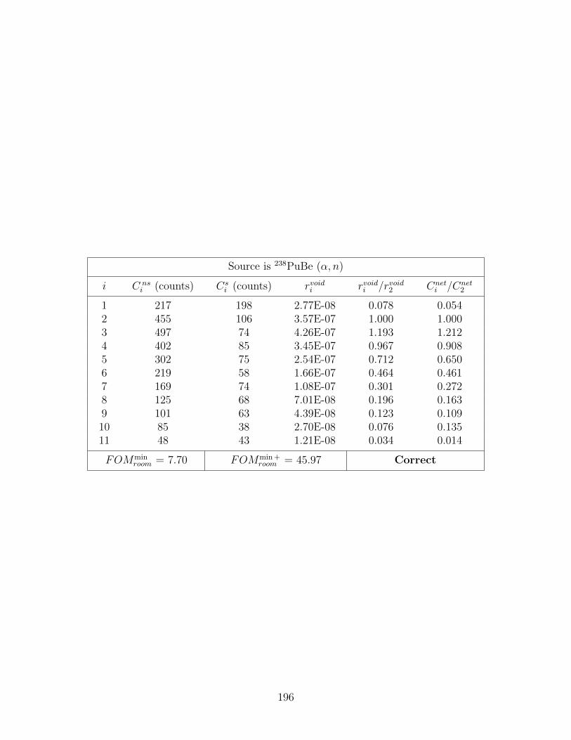
Source is 238PuBe (α, n)
i C nsi (counts) Cs
i (counts) rvoidi rvoidi /rvoid2 Cneti /Cnet
2
1 217 198 2.77E-08 0.078 0.0542 455 106 3.57E-07 1.000 1.0003 497 74 4.26E-07 1.193 1.2124 402 85 3.45E-07 0.967 0.9085 302 75 2.54E-07 0.712 0.6506 219 58 1.66E-07 0.464 0.4617 169 74 1.08E-07 0.301 0.2728 125 68 7.01E-08 0.196 0.1639 101 63 4.39E-08 0.123 0.10910 85 38 2.70E-08 0.076 0.13511 48 43 1.21E-08 0.034 0.014
FOMminroom = 7.70 FOMmin +
room = 45.97 Correct
196
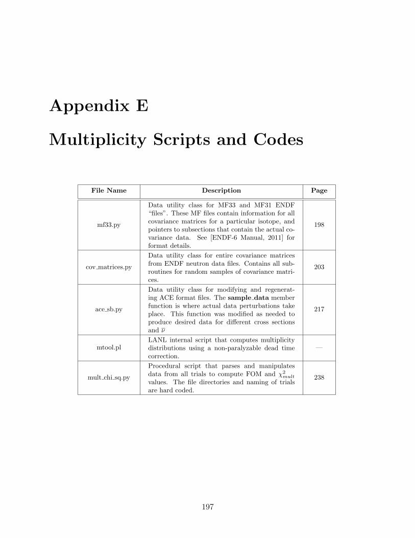
Appendix E
Multiplicity Scripts and Codes
File Name Description Page
mf33.py
Data utility class for MF33 and MF31 ENDF“files”. These MF files contain information for allcovariance matrices for a particular isotope, andpointers to subsections that contain the actual co-variance data. See [ENDF-6 Manual, 2011] forformat details.
198
cov matrices.py
Data utility class for entire covariance matricesfrom ENDF neutron data files. Contains all sub-routines for random samples of covariance matri-ces.
203
ace sb.py
Data utility class for modifying and regenerat-ing ACE format files. The sample data memberfunction is where actual data perturbations takeplace. This function was modified as needed toproduce desired data for different cross sectionsand ν
217
mtool.plLANL internal script that computes multiplicitydistributions using a non-paralyzable dead timecorrection.
—
mult chi sq.py
Procedural script that parses and manipulatesdata from all trials to compute FOM and χ2
mult
values. The file directories and naming of trialsare hard coded.
238
197
mf33.py: Utility Class for ENDF files#!/usr/bin/env python
"Provides methods for working with ENDF102 MF33 Records."
#===================================================================================================
__version__ = "$Id: mf33.py,v 1.9 2012/06/15 23:50:24 morgan Exp $"
#===================================================================================================
# Load local python modules
from ndvv.endf.records.control import controlRecord
from ndvv.endf.records.list import listRecord
from ndvv.log import devnull
from ndvv.endf.records.peek import peek_at_controlRecord
from ndvv.endf.cov_matrices import endfCovMatrix
from math import sqrt
from numpy import zeros, array, diag
#===================================================================================================
class mf33Record(object):
"""This class includes all of the combinations of mt’s (mt1 and mt).
33.2 Formats
Section:
[MAT, 33, MT/ ZA, AWR, 0, MTL, 0, NL] HEAD
<subsection for n = 1>
<subsection for n = 2>
<subsection for n = NL>
[MAT, 33, 0/ 0.0, 0.0, 0, 0, 0, 0] SEND
Subsection:
[MAT,33,MT/ XMF1, XLFS1, MAT1, MT1, NC, NI]CONT
<sub-subsection for n =1>
Sub-subsection:
NI-type:
LB=5: [MAT,33,MT/ 0.0, 0.0, LS, LB=5, NT, NE/ EkFk,k] LIST.
ariables : NT Total number of entries in the two arrays Ek and Fk,k.
NE Number of entries in the array Ek defining (NE-1) energy intervals.
LS Flag indicating whether the F_(k,k’) matrix is symmetric or not.
Definiton of Variables:
AWR - Atomic mass of target ratio to neutron mass
ZA - Atomic number Z*1000 plus atomic mass number A
XMF1 - Floating point equivalent of the MF for the 2nd energy-dependent cross section
of the pair, for which the correlation matrix is given. If MF1=MF,XMF1=0.0 or
blank.
XLFS1 - Floating point equivalent for the final excited state of the 2nd energy dependent
cross section. For MF1=10, XLFS1 = 10; if MF16=10, XLFS1=0.0 or blank.
MAT1 - MAT for the 2nd /energy-dependent cross section
MT1 - MT for the 2nd energy-dependent cross section
NC - Number of NC-type sub-subsections which follow the CONT record.
NI - Number of NI-type sub-subsections which follow the NC-type subsubsections.
MTL - Non-zero value of MTL is used as a flag to indicate that reaction MT is
one component of the evaluator-defined lumped reaction MTL
NL - Number of subsections within a section.
LB - Flag whose numerical value determines the meanings of the numbers given
198

in the arrays Ek, FkEl, Fl.
FOR LB=5:
NP - Total number of pairs of numbers in the arrays Ek, FkEl, Fl.
NT - Total number of numbers in the LIST record; NT=2*NP.
LT - Number of pairs of numbers in the second array, El, Fl.
If LT=0, the table contains a single array Ek, Fk.
If LT not = 0, the table contains two arrays; the first array, Ek, Fk, has
(NP - LT) pairs of numbers in it.
The first line read must contain a valid /MAT,MF,MT/. The loose variable may be used to ignore
subsequent values.
A python logger may be used to capture messages about the data as it is parsed, checked, or
manipulated.
"""
# ---------------------------------------------------------------------------------------------
def __init__(self, f=None, loose=False, logger=None):
"Initialize a MF33 covariance record possibly reading data from f[ile object]."
self.clear()
if f is not None:
self.parse(f=f,loose=loose,logger=logger)
return None
# ---------------------------------------------------------------------------------------------
def clear(self):
"Clear the current record."
self.__dict__[’endfRecords’] = controlRecord()
self.__dict__[’endfCovMatrices’] = [endfCovMatrix()]
return None
# ---------------------------------------------------------------------------------------------
def __getattr__(self, name):
"Override getattr to allow multiple ways of getting record values."
cr = self.__dict__[’endfRecords’]
endfCovMatrices = self.__dict__[’endfCovMatrices’]
d =
’cr’ : ’cr’,
’matmfmt’ : ’cr.mat, cr.mf, cr.mt’,
’mfmt’ : ’cr.mf, cr.mt’,
’mat’ : ’cr.mat’,
’mf’ : ’cr.mf’,
’mt’ : ’cr.mt’,
’za’ : ’cr.c1’,
’awr’ : ’cr.c2’,
’mtl’ : ’cr.l2’,
’nl’ : ’cr.n2’,
value = eval( d.get( name, ’None’ ) )
if value is not None:
return value
raise AttributeError("endf mf33 object has no attribute %s"%(name))
199
#-----------------------------------------------------------------------------------------------
def __setattr__(self, name, value):
"Override setattr to allow multiple ways of setting record values."
cr = self.__dict__[’endfRecords’]
endfCovMatrices = self.__dict__[’endfCovMatrices’]
d =
’matmfmt’ : ’self.mat, self.mf, self.mt = value’,
’mfmt’ : ’self.mf, self.mt = value’,
’mat’ : ’cr.mat= value’,
’mf’ : ’cr.mf=value’,
’mt’ : ’cr.mt= value’,
’za’ : ’cr.c1 = value’,
’awr’ : ’cr.c2 = value’,
’mtl’ : ’cr.l2 = value’,
’nl’ : ’cr.n2= value’
exec( d.get( name, "self.__dict__[name] = value" ) )
return None
# ---------------------------------------------------------------------------------------------
def parse( self, f, loose=False, logger=None):
"Read the MF33 data."
if logger is None:
logger = devnull
logger.log(9,"entered routine ndvv.endf.mf33.parse")
logger.log(8,"%s"%(__version__))
"Read in the head record first:"
cr = controlRecord(f=f, loose=loose, logger=logger)
if (cr.l2 != 0):
raise NotImplemented("There is a lumped reaction sum, not implemented in code yet, see section \
33.2 of ENDF6 Manual for more info")
#TODO
#loop through all the subsections, storing their particular cov matrix data.
covMatrixRecords = []
for subSection in range(cr.n2):
covMatrixRecords.append(endfCovMatrix(f=f, logger=logger, loose=loose))
self.__dict__[’endfCovMatrices’] = covMatrixRecords
self.__dict__[’endfRecords’] = cr
return None
#---------------------------------------------------------------------------------------------
def get_endfCovMatrix(self, mf1=None, mt1=None, mat1=None):
"""Returns the full covariance matrices for a particular mt1 & mf1 (certain subsection record
in the form of cov_matrices class) and corresponding energies. Note
that this is not all one cov matrix, but different pieces seperated by
energy"""
"Look for same mf1 and mat1 and mt1 if there is none specified"
if (mf1 == None):
mf1 = 0.0
if (mat1 == None):
mat1 = 0
if (mt1 == None):
mt1 = self.mt
"get the index of the covariance matrices you want by checking all subsections:"
200

counter = 0
for ss in self.endfCovMatrices:
#put in temp check to make sure no mat1’s different from mat TODO
if (ss.mat1 != 0) or (ss.xmf1 != 0.0):
raise NotImplementedError("There are mf1 and mat1 different from mf and mat")
elif (ss.mt1 == mt1 and ss.mat1 == mat1 and ss.xmf1 == mf1):
return self.endfCovMatrices[counter]
else:
counter += 1
return None
#---------------------------------------------------------------------------------------------
def get_full_matrix(self, mf1=None, mt1=None, mat1=None):
"""Returns a full covariance matrix (covers full energy range). If any entries are None,
the program assumes mf1=mf, or mt1=mt, etc."""
#find the write cov_matrices instance (sub section)
ss = self.get_endfCovMatrix(mf1=mf1, mt1=mt1, mat1=mat1)
#Generate full matrix
return ss.get_full_matrix()
#---------------------------------------------------------------------------------------------
def get_corr_matrix(self, mf1=None, mt1=None, mat1=None):
"""Returns a full covariance matrix (covers full energy range). If any entries are None,
the program assumes the same mat1mf1mt1 as section matmfmt"""
#find the write cov_matrices instance (sub section)
ss = self.get_endfCovMatrix(mf1=mf1, mt1=mt1, mat1=mat1)
#Generate corr matrix
return ss.get_corr_matrix()
#---------------------------------------------------------------------------------------------
def sample_cross_section(self, mf1=None,mt1=None,mat1=None, fi=None, cross_sections=None,
interpolation=None):
"""Samples a vector of ne-1 normally distributed random numbers using Mersenne twister
algorithm and then uses a specified correlation matrix to correlate the random numbers. If
no mf1 or mt1 are specified it is assumed that you want mf1=mf & mt1=mt.
This returns the modified cross sections as an array. WARNING: the fi in this class is not the fi that
this class is associated with, so modifying it will not modify the original fi."""
raise NotImplementedError("This function should work, but I have not explicitly tested it, so be wary."
+"The alg. worked for ACE files so it should be k")
#Generate the right cov_matrices instance (sub section)
ss = self.get_endfCovMatrix(mf1=mf1, mt1=mt1, mat1=mat1)
#Get the correct cross-sections out, noting that by default the mf is just mf - 30
if fi==None:
raise ValueError("Must pass in the file_index object you are working with")
exec("section=fi.get_section(mf=%d, mt=%d)" % (ss.mf-30, ss.mt))
#store cross sections in an array by finding the tab1 record:
endfRecords = section.endfRecords
201

for rec in endfRecords:
if getattr(rec, "line", False): #is it a TAB1 record?
rec.line.y = array(rec.line.y)
cross_sections = array(rec.line.y)
energies = array(rec.line.x)
endfRecord = rec
break
else:
continue
#Sample cross sections using the cov_matrices class
return cov_matrix.sample_cross_section(cross_sections, energies, interpolation)
#==================================================================================================
if __name__ == "main":
#file name and directory of endf file
endf_dir=’/home/sbolding/ENDF_Stuff/CrossX061212/neutrons/’
file_name=’n-094_Pu_239.endf’
# a = mf33Record(file_name)
202
cov matrices.py: Utility Class for ENDF Covariance Ma-
trices#!/usr/bin/env python
"""Provides methods for handling the Covariances matrices specified in 31 and 33 series of files
The subsubsections should really be read out into their own class so that each one will contain
its own energy etc, currnetly they are just lined up by index and two different members of this
class.
Need to be wary that if you were going to reprint these cov matrices to a file the NC
type subsubsections MUST come first. You would need to not sort them by energy.
WARNING: The current version creates the full matrix assuming that each sub_matrix is only for a
particular energy range, if there is overlap it probably won’t work. U235 nubar for example,
this will not work on. I didn’t add it simply because it wasnt in any of my cases.
Need to add logger statements to most of this file"""
#===================================================================================================
__version__ = "$Id: cov_matrices.py,v 1.0 2012/06/15 23:50:24 sbolding $"
#===================================================================================================
# Load local python modules
from ndvv.endf.records.control import controlRecord
from ndvv.endf.records.list import listRecord
from numpy import zeros, matrix
from math import sqrt
from numpy.linalg import cholesky, eig, LinAlgError, norm
from numpy import random, array, diag, transpose, dot, matrix, interp
from scipy import interpolate
#===================================================================================================
class endfCovMatrix(object):
"""This class will hold the information for a subsection from a 30’s series file that contains the
covariance data for a set of cross sections, nubar data, etc. Each instance of this class
contains the covariance matrix (stored as a bunch of submatrices) for a particular mf, mt1, mf1
and mt (subsection). The unique submatrices of the covariance matrix for a particular combination
of mt & mt1 (mostly by energy) are in a list for each instance called by self.covMatrices.
The class mf33 includes all of the combinations of mt’s (mt1 and mt).
EndfFormat Section"""
#-----------------------------------------------------------------------------------------------
def __init__(self, f=None, loose=False, logger=None, seed=None):
"Initialize a Covariance Matrix record"
self.clear()
#Initialize random number generator to arbitrary value
random.seed(self.seed)
if f is not None:
self.f = f
self.parse(f=f, loose=loose, logger=logger)
return None
#-----------------------------------------------------------------------------------------------
def clear(self):
203

"Clear the current record."
self.__dict__[’endfRecords’] = tuple([controlRecord(), listRecord()])
self.__dict__[’covMatrices’] = [] #contains the portions of covariance matrices for each case
# each member of the list ’covRecords’ is a full matrix
# that makes up some portion of a particular section. I
# think the portions have to do with energy, but i can’t
# tell for sure.
self.__dict__[’energies’] = [] #contains the energy bins for the corresponding covmatrix
self.__dict__[’sorted’] = False #is the data sorted in order of increasing energy?
self.relative = False #Is the cov matrix relative (vs absolute)?
self.f = None #File object
self.modified_corr_matrix = None #If a fixup is applied, a new correlation matrix is stored
self.sampling_matrix = None #The matrix used for sampling is stored
self.full_matrix = None #2d array that is the original full matrix, ignoring modifications
self.fixup_applied = False #If a fixup has been applied or not, may not be used
self.seed = 17
return None
#----------------------------------------------------------------------------------------------
def __getattr__(self, name):
"Override getattr to allow multiple ways of getting section values."
cr = self.__dict__[’endfRecords’][0]
lrs = self.__dict__[’endfRecords’][1:] #list of the list records
d =
’cr’ : ’cr’,
’matmfmt’ : ’cr.mat, cr.mf, cr.mt’,
’mfmt’ : ’cr.mf, cr.mt’,
’mat’ : ’cr.mat’,
’mf’ : ’cr.mf’,
’mt’ : ’cr.mt’,
’nc’ : ’cr.n1’,
’ni’ : ’cr.n2’,
’mat1’ : ’cr.l1’,
’mt1’ : ’cr.l2’,
’xmf1’ : ’cr.c1’,
’xlfs1’ : ’cr.c2’
value = eval(d.get(name,’None’))
if value is not None:
return value
raise AttributeError("endf covariance matrices object has no attribute %s"%(name))
#-----------------------------------------------------------------------------------------------
def __setattr__(self, name, value):
"Override setattr to allow multiple ways of setting record values."
cr = self.__dict__[’endfRecords’][0]
lrs = self.__dict__[’endfRecords’][1:] #list of the list records
d =
’cr’ : ’cr=value’,
’matmfmt’ : ’cr.mat, cr.mf, cr.mt=value’,
’mfmt’ : ’cr.mf=value’,
’mat’ : ’cr.mat=value’,
’mf’ : ’cr.mf=value’,
’mt’ : ’cr.mt=value’,
’nc’ : ’cr.n1=value’,
’ni’ : ’cr.n2=value’,
’mat1’ : ’cr.l1=value’,
’mt1’ : ’cr.l2=value’,
’xmf1’ : ’cr.c1=value’,
’xlfs1’ : ’cr.c2=value’
204

exec( d.get( name, "self.__dict__[name] = value" ) )
return None
#----------------------------------------------------------------------------------------------
def parse(self, f, loose=False, logger=None):
"Parses all sub and sub-sub section data and stores them into matrices and Records"
if logger is None:
logger=devNull
logger.log(9,"entered routine ndvv.endf.cov_matrices.parse")
logger.log(8,"%s"%(__version__))
"Read in the header of the sub section"
cr = controlRecord(f) #Control record for a single covariance matrix/single subsection
endfRecords = [cr]
#set subSection values
ni = cr.n2
nc = cr.n1
xmf1 = cr.c1
if (xmf1 != 0.0):
raise ValueError("There is a dependence on another MF, this is not coded. See the"+ \
"manual section 33.2.1")
#Temp Variables for storing after iteration into tuples:
covMatrices = []
energies = []
for nc in range(nc):
if nc > 0:
raise ValueError("Need to put in code to read in NC type sub-subsections")
#TODO
for ni in range(ni): #read in all of the NI sub-subsections
lr = listRecord(f)
lb = lr.l2 #type of cross section
logger.log(9,"entering code that parses the subsubsection matrices")
#------------------------------------------------------------------------------------
"Parse the subsubsection matrices"
#------------------------------------------------------------------------------------
if (lb not in [5]):
msg = "Need to put in code to read in LB=%d format NI sub-subsections" % lb
raise NotImplementedError(msg)
elif lb == 5:
"Direct matrix data section"
self.relative = True
ls = lr.l1 #symmetric or not
nt = lr.npl #total number of entries in lr.b
ne = lr.n2 #number of energies
m = zeros([ne-1,ne-1]) #create matrix to store data
erg = lr.b[0:ne] #store list of energies
205
if ls == 1:
"Read in an upper triangular (symmetric) format matrix:"
"Store the matrix elements:"
index=ne #start of b_n elements
for i in range(ne-1):
for j in range(i,ne-1):
m[i][j] = lr.b[index]
#Don’t overwrite diagonal element
if (j != i):
m[j][i] = lr.b[index]
index+=1 #increment location on data list
elif ls==0:
"Read in a full (asymmetric) matrix"
msg = "Warning, you have read in an asymmetric covariance matrix...whatever that " \
+"means, for mt1=%d, subsubsection #%d. See ENDF manual chpt 33 for more"\
% (cr.l2, len(covMatrices))+"info. May not actually be asymmetric, use"\
+" cov_matrices.symmetric to check\n"
print msg
logger.log(9,msg) #NOT SURE IF THIS IS THE RIGHT FORMAT TODO"
"Store the matrix elements:"
index=ne #start of b_n elements
for i in range(ne-1):
for j in range(ne-1):
m[i][j] = lr.b[index]
index+=1 #increment locatioon in list
else:
raise ValueError("Incorrect value for LS on an LB=5 card")
"Store the data after it is read in:"
energies.append(erg)
covMatrices.append(m)
endfRecords.append(lr)
"Store all data to instance:"
self.__dict__[’covMatrices’]=covMatrices
self.__dict__[’energies’]=energies
self.__dict__[’endfRecords’] = tuple(endfRecords)
return None
#-----------------------------------------------------------------------------------------------
def check(self):
#TODO
print """Need to write checks to make sure mf1 mt1 mat1 all the same for a particular
instance"""
#-----------------------------------------------------------------------------------------------
def get_full_matrix(self):
"""Returns a full matrix for a particular subsection (one covMatrices class). This requires
making the matrix out of its various energy components. The correct MT1 and MF1/Mat1 are
specified in higher class mf33Record"""
if self.full_matrix != None:
return self.full_matrix
206
"If the measurement is relative warn user:"
if self.relative == True:
print "WARNING: the covariance matrix you are using is for relative covariances"+ \
", the correlation matrix is correct and does not need to be changed"+\
". See ENDF Chapter 33.2.2.2\n"
#Sort energies if not already done:
if not self.sorted:
self.sort_by_energy()
#Determine the total number of energies:
energies = self.get_energies()
ne = len(energies)
#Create Matrix:
m = zeros([ne-1,ne-1])
xidx = 0
yidx = 0
counter=0
skip_cycles=0
for k in range(len(self.covMatrices)):
yidx_initial = xidx
for i in range(len(self.covMatrices[k])):
#Set col location in m to start at the location of where rows being changed start
yidx = yidx_initial
for item in range(len(self.covMatrices[k][i])):
if (k != 0):
#for the first cov matrix you just print the whole thing
if (item == 0) or ( i == 0):
#for higher k you need to skip the first entry in row and column
continue
m[xidx][yidx] = self.covMatrices[k][i][item]
yidx += 1
#Increment location in m after each row
if (i == 0 and k != 0):
continue
else:
xidx += 1
# CHECK MATRIX VALUES:
if not symmetric(m):
raise ValueError("Non-symmetric cov matrix, need to add code to accounts for this")
"""
print m[55][45], self.covMatrices[0][55][45]
print m[len(self.covMatrices[0])-1][len(self.covMatrices[0][0])-1], self.covMatrices[0][-1][-1]
print m[-1][-1], self.covMatrices[1][-1][-1]
print m[-4][-3], self.covMatrices[1][-4][-3]
print m[len(self.covMatrices[0])][len(self.covMatrices[0])], self.covMatrices[1][1][1]
"""
self.full_matrix = m
return m
#-----------------------------------------------------------------------------------------------
207
def get_energies(self):
"""Determine the total list of energies for this subsection. This data is in the endfRecords for a
cross section, but this class doesn’t have access to that data. I am not totally sure how
it stores the different sections, so it may be better to not duplicate by brute force"""
#Make sure in order of increasing energy:
if not self.sorted:
self.sort_by_energy()
#append non duplicate energies to the list [0,1,2,..,m,m+1,...,p,p+1...q-1,q]:
erg = []
for eng in range(len(self.energies)):
temp = self.energies[eng]
#The lowest one covers the full range of its energies [0,1, 2,..,m]
if eng == 0:
erg.extend(self.energies[eng])
#The Last one has a duplicate has two duplicates on its lower end [0,p,p+1,...q]:
elif eng == (len(self.energies)-1):
erg.extend(self.energies[eng][2:])
#Middle ones lose two to their bottom as well as a top energy [0,m,m+1,..,p-1,p,q]:
else:
erg.extend(self.energies[eng][2:])
return erg
#-----------------------------------------------------------------------------------------------
def sort_by_energy(self):
"""Need to be wary that if you were going to reprint these cov matrices to a file the NC
type subsubsections MUST come first. You would need to not sort them by energy"""
#sort in order of ascending energy
#put in debug error:
if(len(self.energies) > 2):
raise NotImplementedError("Has not been tested on data that has more than 2"
+"subsubsections,make sure energies and matrix have values for all energies ")
#create a list of data that can be sorted
if (len(self.energies) != len(self.covMatrices)):
raise ValueError("Somehow the number of energy arrays is different from the no. of matrices")
matrix_data = []
for erg in range(len(self.energies)):
matrix_data.append(tuple([self.energies[erg], self.covMatrices[erg],
self.endfRecords[erg+1]]))
#put in order of increasing energy range
matrix_data = sorted(matrix_data, key=lambda top_energy: top_energy[0][-1])
#Store sorted data back to instance data
self.energies = []
self.endfRecords = [self.__dict__[’endfRecords’][0]]
self.covMatrices = []
for erg in range(len(matrix_data)):
self.energies.append(matrix_data[erg][0])
self.endfRecords.append(matrix_data[erg][2])
self.covMatrices.append(matrix_data[erg][1])
self.sorted = True
self.__dict__[’endfRecords’] = tuple(self.__dict__[’endfRecords’])
return None
208
#-----------------------------------------------------------------------------------------------
def get_corr_matrix(self):
"Generates a correlation matrix for a particular subsection"
#First generate the covariance matrix
m = self.get_full_matrix()
corr = zeros([len(m), len(m[0])])
for i in range(len(m)):
for j in range(len(m)):
if (m[i][j] == 0.0):
corr[i][j]=0.0
else:
corr[i][j] = m[i][j]/(sqrt(m[i][i]*m[j][j]))
return corr
#-----------------------------------------------------------------------------------------------
def gen_sampling_matrix(self, m=None):
"""Returns a sampling matrix for generating correlated random samples. m (cov matrix) can be
specified. This is primarily for debugging and external use of this function"""
#Get the correct correlation matrix and check for symmetry:
if m==None:
m = self.get_corr_matrix()
#Check that none of the variances are zero, and if so store row and raise flag:
zero_variances = []
cov = self.full_matrix
for i in range(len(self.full_matrix)):
if cov[i][i] == 0.0:
print "Zero variance in correlation matrix, setting row/column to zero in sampling matrix"
zero_variances.append(cov[i][i])
#Check that all columns and rows of this one are zero:
for j in range(len(cov)):
if cov[i][j] != 0.0 or cov[j][i] != 0.0:
raise ValueError("There is zero variance, but non zero covariance...not possible")
#Remove the zero_variance rows and columns from the correlation matrix
if zero_variances != []:
temp_m = []
for i in range(len(m)):
if i in zero_variances:
continue
else:
temp_list = []
for j in range(len(m[i])):
if j in zero_variances:
continue
else:
temp_list.append(m[i][j])
temp_m.append(temp_list)
m = array(temp_m)
try:
#See if positive definite and cholesky decomposition will work (much more efficient)
if not symmetric(m):
209
raise LinAlgError("WARNING: non symmetric matrix")
print "\nChecked if matrix was symmetric or not..."
u = cholesky(m) #Will raise LinAlgError if it fails
except LinAlgError:
#Try eigenvalue decomposition
print "Not positive definite, trying singular Eigenvalue decomposition..."
evals, evecs = eig(m)
#Check for negative eigenvalues, if so, then need to make a PSD correlation matrix:
check = all(eval >= 0.0 for eval in evals)
zero_check = all(eval != 0.0 for eval in evals)
if not zero_check:
raise LinAlgError("There is a zero eigenvalue, need to account for this")
if not check:
print "Negative eigenvalues, indefinite matrix, applying Eigenvalue Fixup Method..."
m = self.eigenvalue_fixup(evals, evecs) #returns a new corr matrix that is PSD
print "Fixup applied"
evals, evecs = eig(m)
#make sure nothing failed in fixup
check = all(eval > 0 for eval in evals)
if not eigenmatrix_check(evals,evecs):
raise LinAlgError("Error in new eigenvector decomposition matrix")
if not check:
raise LinAlgError("Still have neg. eigenvalues, even after fixup method")
if not eigenmatrix_check(evals,evecs):
raise LinAlgError("Error in final eigenvector decompositon result")
#Generate u
sqrt_evals = []
for i in evals:
sqrt_evals.append(sqrt(i))
u = dot(evecs, sqrt_evals)
#If there were zero variances u need to set those values in sampling matrix to zero:
if zero_variances != []:
temp_m = []
x_idx = 0
for i in range(len(cov)):
temp_list = []
y_idx= 0
for j in range(len(cov[i])):
if j in zero_variances or i in zero_variances:
temp_list.append(0.0)
else:
temp_list.append(u[x_idx][y_idx])
y_idx+=1
210
if j in zero_variances:
y_idx -= 1
if i in zero_variances:
x_idx -= 1
temp_m.append(temp_list)
x_idx += 1
u = array(temp_m)
self.sampling_matrix = u
return None
#---------------------------------------------------------------------------------------------------
def eigenvalue_fixup(self, evals, evecs):
"""Fixup applied to correlation matrices with negative eigenvalues that are not semi-positive
definite. This method works by setting all the eigenvalues to positive and then generating
a new correlation matrix with a fixed set of values
This function returns the modified eigenvector matrix, but it stores the modified
correlation matrix to self.modified_corr_matrix for access later"""
#Check to make sure that the matrix is orthogonal etc. before applying fixup
if not eigenmatrix_check(evals, evecs):
raise LinAlgError("Need to apply Gramm-Schmidt method, not implemented")
#Make a new array of positive evals
pos_evals = []
for i in evals:
pos_evals.append(abs(i))
pos_evals = array(pos_evals)
#make diagonal matrix of pos eigenvalues:
d = matrix(diag(pos_evals))
#solve for new correlation matrix, use matrix module to simplify multiplication
tr = matrix(evecs.transpose())
emat = matrix(evecs)
new_corr = emat*d*tr
new_corr = array(new_corr)
#Need to make sure diagonal elements are 1. In most cases they will not be:
dd = diag(new_corr)
for i in range(len(new_corr)):
for j in range(len(new_corr)):
new_corr[i][j] = new_corr[i][j]/(sqrt(dd[i]*dd[j]))
self.modified_corr_matrix = new_corr
#check that new correlation matrix is normalized
for i in range(len(new_corr)):
if abs(new_corr[i][i] - 1.0) > 0.000001:
raise LinAlgError("Something has gone wrong in renormalizing the new corr matrix")
#return the modified correlation_matrix
return new_corr
#---------------------------------------------------------------------------------------------------
def sample_corr_matrix(self, seed=None):
"""samples a set of normally distributed random numbers from a correlation matrix. Uses
self.sampling_matrix if there is one, else reads it in using self.gen_sampling_matrix.
211

Returns correlated samples from a normal distribution with mean of zero and std deviation of one
The random seed can be specified here, or it uses the one stored. Self.seed is updated
BEFORE this function is ran. This is for storing the seed that generated each set of sampled
data external to this class"""
if self.sampling_matrix == None:
self.gen_sampling_matrix()
#Generate a vector of random numbers, distributed normally: use specified seed if one is given
if seed != None:
random.seed(seed)
self.seed = random.get_state()[1][0]
#Get the sampling matrix: sample_mat = self.sampling_matrix
#Generate normally distributed random numbers rand_array =
array(random.randn(len(sample_mat)))
#Sample 1000 numbers from the random number generator, this is so it
#jumps ahead in the period and the seed will be changed. The seed only
#changes every #623 samples because mersenne twister smaples 623 numbers
#at each state. This is much easier than trying to store
#the whole state. 1000 is arbitrary, and numbers were checked to be random
random.randn(1000)
#multiplication by hand
temp_array = []
for i in range(len(sample_mat)):
sum = 0.
for j in range(len(sample_mat[i])):
sum += sample_mat[i][j]*rand_array[j]
temp_array.append(sum)
temp_array = array(temp_array)
return temp_array
#-----------------------------------------------------------------------------------------------
def sample_cross_section(self, cross_sections, energies, seed=None, interpolation=None):
"""Samples a vector of ne-1 normally distributed random numbers using Mersenne twister
algorithm and then uses a specified correlation matrix to correlate the random numbers.
The energies in the input are those of the crossX, not those of the cov matrix.
The energies of the crossx are typically different than those of the cov matrix, therefore
the random numbers generated from the cov matrix have to be mapped onto the cross sections.
The cov matrix values are group averaged.
If any of the variances are zero, that cross section is not sampled and returned as the original
value and there is no correlation to it."""
#sample rand_array (generating sample matrix if one not already specified)
rand_array = self.sample_corr_matrix(seed=seed)
cov_energies = array(self.get_energies())
#Get out the std_dev into an array
cov = self.get_full_matrix()
std_dev = array([ sqrt(cov[i][i]) for i in range(len(cov))])
#If any of the variances are zero they will be canceled out by the way the corr_matrix is set up
212

#Map the variances on to the proper cross sections due to different numbers of energy pnts:
mapped_rand_array = []
mapped_std_dev= []
cov_idx = 0
#This next section makes a vector of correlated values that is same size as the number of cross sections
#by mapping values based on energies. The correlation matrix is for group averaged values, so if
#a cross section falls within that group, it is set to have the same relative variance/covariance
#that group corresponds to.
# - - - - - - -- - - - - - - - -- - - - - - - -- -- - - - - - - -- -- - - - - - - -- -- - - - - - - -
if not self.relative:
raise ValueError("The mapping of energies in this function only works for relative covariance data,"
+" need to rewrite if not relative")
#raise error if different endpoint energies
if abs(cov_energies[-1] - energies[-1]) > 0.000001:
print cov_energies[-1], energies[-1]
raise ValueError("Different Upper Endpoint Energies b/w cov and CX data, handling this case not "
+"implemented yet. Possible that energies of crossX not in eV, as they are in the cov data")
for i in range(len(energies)-1):
while True:
if (energies[i] - cov_energies[cov_idx]) >= -0.0000000001:
if (cov_energies[cov_idx+1] - energies[i]) > -0.0000000001:
#in the proper energy bin
mapped_rand_array.append(rand_array[cov_idx])
mapped_std_dev.append(std_dev[cov_idx])
break
else:
cov_idx+=1
else:
if cov_idx == 0:
#handle case where the cross sections have starting energies lower than the
#covariance data by setting the sampling of all cross sections below that value to 0.0.
#This effectively means no changes are made to those cross sections
mapped_rand_array.append(0.0)
mapped_std_dev.append(0.0)
raise ValueError("You probably shouldnt need this, make sure it’s actually how"
+"you want to handle this data. More details in source")
break
else:
raise ValueError("Energies got out of order somehow")
#Store the last case which is always the last variance
mapped_rand_array.append(rand_array[-1])
mapped_std_dev.append(std_dev[-1])
mapped_rand_array = array(mapped_rand_array)
mapped_std_dev = array(mapped_std_dev)
if self.relative:
mapped_std_dev = mapped_std_dev*cross_sections
#Generate modified cross section data
cx = mapped_rand_array*mapped_std_dev + cross_sections
#Use interpolation if desired
213
print interpolation
if interpolation != None:
return self.inter_cross_section(cx, energies, interpolation=interpolation)
else:
#DEBUG
temp_file = open("/scratch/sbolding/nubar_plot.txt","w")
for i in range(len(cx)):
temp_file.write("%s %s %s\n" % (energies[i], mapped_rand_array[i], mapped_std_dev[i]))
return cx
#-----------------------------------------------------------------------------------------------
def inter_cross_section(self, cross_sections, energies, interpolation="linear"):
"""Function reads in a set of sampled cross sections and adjusts them such that the center of each
cov energy group is the sampled value and in between some kind of interpolation method is used.
By default linear interpolation is assumed."""
#input check
if len(cross_sections) != len(energies):
raise ValueError("Length of cross sectios and energies do not match")
#intialize local variables
cov_energies = self.get_energies()
centered_cx = []
centered_energies = []
#find center point (or slightly lower energy) of each cov energy group and store cx and energy.
avg_energies = []
for i in range(len(cov_energies)-1):
avg_energies.append((cov_energies[i] + cov_energies[i+1])/2.)
#map centerpoints to energies and cross section values
idx = 0
for cx in range(len(cross_sections)):
if energies[cx] < avg_energies[idx]:
continue
elif energies[cx] >= avg_energies[idx]:
#Check to see if one above or below is closest
check_hi = abs(energies[cx] - avg_energies[idx])
check_low = abs(energies[cx-1] - avg_energies[idx])
if check_hi < check_low:
centered_cx.append(cross_sections[cx])
centered_energies.append(energies[cx])
else:
centered_cx.append(cross_sections[cx-1])
centered_energies.append(energies[cx-1])
idx += 1
if idx == len(avg_energies):
break
#add first and last value of cross_section and energy to make interpolation easier
centered_cx.insert(0, cross_sections[0])
centered_cx.append(cross_sections[-1])
centered_energies.insert(0, energies[0])
214
centered_energies.append(energies[-1])
#perform interpolation
if interpolation == "linear":
cx = interp(energies, centered_energies, centered_cx)
for i in range(len(cx)):
print energies[i], cross_sections[i], cx[i]
# for j in range(len(centered_energies)):
# print centered_energies[i], centered_cx[i]
exit()
return cx
elif interpolation == "cubic_spline":
tck = interpolate.splrep(centered_energies, centered_cx)
cx = interpolate.splev(energies, tck)
for i in range(len(cx)):
print cx[i]
exit()
return cx
else:
raise ValueError("Invalid, or unimplimented, entry for interpolation scheme")
exit() #STILL DEBUGGING
return cross_sections
#---------------------------------------------------------------------------------------------------
def eigenmatrix_check(evals, evecs):
"""Checks an eigenmatrix to ensure all columns are orthogonal and normalized to one
and that there are no degenerate eigenvalues. Need to be careful, lots of potential issues with
roundoff accumulation.
Prints out any errors to the screen, and returns False if any tests failed"""
TOL = 1.0e-05
no_errors = True
#CHeck for degenerate eigenvalues and zero eigenvalues
for i in range(len(evals)):
if evals[i] == 0.0:
print "Zero valued eigenvalue"
no_errors = False
for j in range(i,len(evals)):
if i != j:
if evals[i] == evals[j]:
print "Degenerate Eigenvalues, matrix will not be orthogonal", evals[i], evals[j]
no_errors = False
215

#Check for normalization of eigenvectors
for i in range(len(evecs)):
check = abs(norm(evecs[:][i]) - 1.0)
if check > TOL:
print "Not very-well normalized, most likely do to round off: norm = ",norm(evecs[:][i])
raise ValueError("Not normalized, may just be round off")
#Check for orthogonality of eigenvectors:
for i in range(len(evals)):
for j in range(len(evals)):
if i != j:
dp = dot(evecs[:][i],evecs[:][j])
if abs(dp) > TOL:
print "Not orthogonal for columns ", i, " and ", j, "dp = ", dp
no_errors = False
return no_errors
#---------------------------------------------------------------------------------------------------
def symmetric(m):
"""Check to see if a matrix is symmetric or not. Returns True if symmetric, else False"""
return all(all(float(m[i,j]) == float(m[j,i]) for j in range(i,len(m[i])))for i in range(len(m)))
216

ace sb.py: ACE Format Data Class
#!/usr/bin/env python
#!/home/sbolding/EPD/epd-7.3-1-rh5-x86_64/bin/python
# ===============================================================
#Local Modules
from numpy import array
from math import sqrt
import os
import linecache
#Module for reading in covariance data
from ndvv.endf.file_index import file_index
# ===============================================================
"""This module creates an ace file object from an ace file and contains
strategies for reading in a section from the file and reprinting a new ace file.
NOTE: If you change any of the cross sections stored in "self.data_arrays" in this file
it will be changed when you use fprint. To access the original data need to use
"self.orig_data_arrays".
NOTE: The indexing in this program typically starts from 0, but the ACE format
is based on starting from 1. At times this can be confusing, particularly with
line_cache.getline() and some of the get_array_element functions. In all cases the
values in this program are THE VALUE IN ACE FORMAT MANUAL - 1 so that they are indexed from 0
UPDATE 09/25/12: You can now change cross sections, not just nubar. All data is stored in
parrallel arrays and then accessed by an index. The indices are mapped using self.indices
dictionary and the names desired."""
# = = = = = = = = = = = = = = = = = = = = = = = = = = =
class ace_file_index:
"""This super class contains the files and such needed for parsing and to be used for printing etc.
Also contains the ace sections that have been called and changed"""
def __init__(self, section, xsdir_handle=None, output=None, dir=None):
#get rid of the old data
self.file_index_clear()
if dir == None:
#assume current directory
self.dir = os.curdir
else:
self.dir=dir
#open output file
if output==None:
print "must read in output file name later"
else:
self.output=output
self.__dict__[’outfile’] = open(self.output,"w")
self.section = section
#No XSDIR file:
if xsdir_handle == None:
217

raise IOError("need to specify a XSDIR file")
#XSDIR FILE READ
if xsdir_handle != None:
self.xsdir = open(self.dir+xsdir_handle, "r")
#Find line that has the file you need
flag=False
for line in self.xsdir:
if search_for(section, line):
flag=True #This is purely for reading the next line
#store section_info and initiate input file
self.sectionRecord = tuple(line.split())
#Check to see if endf file is not in current directory
if self.sectionRecord[4] == ’1’:
self.f_handle = self.dir+self.sectionRecord[2]
else:
if not search_for(self.sectionRecord[4], "$(/\s*"):
self.f_handle = self.sectionRecord[4]+"/"+self.sectionRecord[2]
else:
self.f_handle = self.sectionRecord[4]+self.sectionRecord[2]
raise NotImplementedError("This has not been debugged")
self.f = open(self.f_handle, "r")
if self.sectionRecord[0] != self.section:
raise IOError("Read in incorrect line in xsdir file")
elif flag:
#Get the stopping address from next line
self.stop_address = int(line.split()[5])
flag=False
return None
# - - - - - - - - -- - -- - - - - - - - - - - - - - -
def file_index_clear(self):
self.f = None #input ACE file that is being read in and modified
self.xsdir = None #xsdir file
self.xsdir_handle = None #name of xsdir file
self.output = None #name of output file
self.outfile = None #output file
self.of_idx = None #Line in output file
self.of_col = None #col in output file
self.dir = None #directory location of xsdir (and possible f)
self.section = None #The name of the section being modified, e.g. "94239.70c"
self.sectionRecord = None #Contains information about the section, such as location in f
self.f_handle = None #name of f
self.mod_secs = [] #list of classes containing all the info u need for new file
self.stop_address = None #The start of the next cross section data, when to stop printing
self.fi_object = None #File index object, has to do with getting covariance matrices
return None
218
# - - - - - - - - -- - -- - - - - - - - - - - - - - -
def lc_get_lines(self, fileName, start, nolines):
"returns a list of lines gotten using the get_lines function"
idx = start
lines = []
for i in range(nolines):
lines.append(linecache.getline(fileName, idx))
return lines
# = = = = = = = = = = = = = = = = = = = = = = = = = = = = = =
class ace_section(ace_file_index, object):
"""Contains the data for a particular section from an ace file"""
# - - - - - - - - -- - -- - - - - - - - - - - - - - -
def __init__(self, section, section_type, xsdir_handle = None, output=None, dir=None):
self.section_clear()
ace_file_index.__init__(self, section, xsdir_handle=xsdir_handle, output=output, dir=dir)
self.type = section_type
if self.f != None:
self.parse()
else:
raise ValueError("trouble opening input file from xsdir line")
return None
# - - - - - - - - -- - -- - - - - - - - - - - - - - -
def __getattr__(self, name):
#Cr is just a local variable for quick reference
cr = self.__dict__[’controlData’]
d =
’nu_ne’ : ’int(cr[3])’,
’lnu’ : ’int(cr[1])’,
’knu’ : ’int(cr[0])’,
’nr’ : ’int(cr[2])’,
’totnu’ : "self.__dict__[’data_arrays’][1]",
’promptnu’: "self.__dict__[’data_arrays’][0]"
value = eval( d.get( name, ’None’ ) )
if value is not None:
return value
raise AttributeError("ace_section object has no attribute %s"%(name))
# - - - - - - - - -- - -- - - - - - - - - - - - - - -
def __setattr__(self, name, value):
#Cr is just a local variable for quick reference
cr = self.__dict__[’controlData’]
d =
’nu_ne’ : ’cr[3]=value’,
’lnu’ : ’cr[1]=value’,
’knu’ : ’cr[0]=value’,
’nr’ : ’cr[2]=value’
219
exec( d.get( name, "self.__dict__[name] = value" ) )
return None
# - - - - - - - - -- - -- - - - - - - - - - - - - - -
def parse(self, f=None):
#parse file from superClass
if f == None:
f = self.f
fileName = self.f_handle
print "Parsing section..."
#Store relavent line info:
sr = tuple(self.sectionRecord)
self.address =int(sr[5])
self.table_length = sr[6]
self.idx = int(self.address) #index of where you are in the file
#++++++++++ Parse different types of data +++++++++++++++++++++
if self.type == "totnu" or self.type == "promptnu": #Need to parse both the totnu and promptnu data
#Get the relative location of the nubar data and figure out how much offset:
line_offset = self.get_jxs_value(1) #no. of data entries to skip from end of information block
if line_offset == "0":
raise ValueError("No nuBar data")
#there are 4 data entries per line and 12 lines of control information at the start:
self.data_addresses.append(int(line_offset/4)+ self.address + 12)
self.idx = int(self.data_addresses[-1]) #update the index
self.data_offset_col= line_offset % 4 #column # @ for the beggining of data
self.col = int(self.data_offset_col)
self.data_offsets.append(self.col)
#Read in the controlData:
self.controlData = self.get_data_points(4,update=True)
if self.knu < 0:
#Parse the total and fast nubar stuff
if self.lnu != 2:
raise ValueError("Coefficient stuff, dont have code to handle this yet")
#Read in the energies and the prompt nubar stuff efficiently
energies = []
for i in range(self.nu_ne):
energies.append(float(self.get_line_data_point(update=True)))
self.energies = array(energies)
#Read in the prompt nubar data
#Store the starting place of a modified section:
self.start_changes.append(tuple([self.idx, self.col]))
data_array = []
for i in range(abs(self.knu) - len(self.controlData) - self.nu_ne + 1):
data_array.append(float(self.get_line_data_point(update=True)))
self.data_arrays.append(array(data_array))
#Store the data_arrays as read in so u can access the original data when sampling
self.orig_data_arrays.append(array(data_array))
#Store the stopping place for data
self.stop_changes.append(tuple([self.idx, self.col]))
220
#Read in the next control data temporarily and store data indexing locations
self.data_addresses.append(self.idx)
self.data_offsets.append(self.col)
cr = tuple(self.get_data_points(3, update=True))
#Checks:
if int(cr[2]) != self.nu_ne:
raise ValueError("Different number of energies for prompt and total")
if int(cr[0]) != 2:
raise ValueError("Coefficient stuff, dont have code to handle this yet")
#Read in energies just to check
energies = []
for i in range(self.nu_ne):
energies.append(float(self.get_line_data_point(update=True)))
#Make sure energies are teh same:
if energies[-1] != self.energies[i]:
raise ValueError("Energy arrays are not the same for total and prompt nubar")
del energies
#Store starting place of next set of data:
self.start_changes.append(tuple([self.idx, self.col]))
#Read in the total nubar data
data_array = []
for i in range(self.nu_ne):
data_array.append(float(self.get_line_data_point(update=True)))
#store data and stopping point of data changes
self.data_arrays.append(array(data_array))
#Store the data_arrays as read in so u can access the original data when sampling
self.orig_data_arrays.append(array(data_array))
self.stop_changes.append(tuple([self.idx, self.col]))
#Store what the index is for total and prompt nubar:
self.data_indices["totnu"] = len(self.data_arrays) - 1
self.data_indices["promptnu"] = len(self.data_arrays) - 2
else:
raise NotImplementedError("need to add stuff to get just total or just fast nubar data")
elif self.type == "capture" or self.type == "total" or self.type == "fission":
#You have to read in the total to adjust capture or fission
print "Warning: This function adjusts the total absorption or fission"+
", and elastic scattering cross section to compensate for the increase."
+"This does not adjust the individual components of the absorption cross section"
+" (such as radiative capture) or individual fission components"""
#Get energy table, which starts at JXS(1):
self.go_to_xss(self.get_jxs_value(0))
ne = self.get_nxs_value(2) #number of energies
energies = []
for erg in range(ne):
energies.append(float(self.get_line_data_point(update=True)))
self.energies = energies #energies for the total, capture, or elastic cxs
#Read in the total cross section
#Store the starting place of a modified section for total:
self.start_changes.append(tuple([self.idx, self.col]))
221
data_array = []
for i in range(ne):
data_array.append(float(self.get_line_data_point(update=True)))
#store data and stopping point of data changes
self.data_arrays.append(array(data_array))
#Store the data_arrays as read in so u can access the original data when sampling
self.orig_data_arrays.append(array(data_array))
self.stop_changes.append(tuple([self.idx, self.col]))
#update data_index for total
self.data_indices["total"] = len(self.data_arrays)-1
#Read in the capture cross section
#Store the starting place of a modified section for total:
self.start_changes.append(tuple([self.idx, self.col]))
data_array = []
for i in range(ne):
data_array.append(float(self.get_line_data_point(update=True)))
#store data and stopping point of data changes
self.data_arrays.append(array(data_array))
#Store the data_arrays as read in so u can access the original data when sampling
self.orig_data_arrays.append(array(data_array))
self.stop_changes.append(tuple([self.idx, self.col]))
#update data_index for capture
self.data_indices["capture"] = len(self.data_arrays)-1
#Read in the elastic cross sections
self.go_to_xss((self.get_jxs_value(0)+3*ne))
print self.idx, self.col
#Store the starting place of a modified section for total:
self.start_changes.append(tuple([self.idx, self.col]))
data_array = []
for i in range(ne):
data_array.append(float(self.get_line_data_point(update=True)))
#store data and stopping point of data changes
self.data_arrays.append(array(data_array))
#Store the data_arrays as read in so u can access the original data when sampling
self.orig_data_arrays.append(array(data_array))
self.stop_changes.append(tuple([self.idx, self.col]))
#update data_index for total
self.data_indices["elastic"] = len(self.data_arrays)-1
#-------------------------------------------------------------------
#Read in the fission cross section
fis = self.get_jxs_value(20)
if int(fis) == 0:
raise IOError("There is no FIS block for this file")
# go to start of fis block and check ne is same as ESZ grid
self.go_to_xss(fis)
ie = int(self.get_line_data_point(update=True))
if ie != 1:
raise ValueError("The first value in the table is not that of the first energy point"
+", you need to change the code to handle this case, see manual_volIII page F-33")
222
num_entries = int(self.get_line_data_point(update=True))
if num_entries != ne:
raise ValueError("Have read in the wrong data block")
self.start_changes.append(tuple([self.idx, self.col]))
data_array = []
for i in range(ne):
data_array.append(float(self.get_line_data_point(update=True)))
#store data and stopping point of data changes
self.data_arrays.append(array(data_array))
#Store the data_arrays as read in so u can access the original data when sampling
self.orig_data_arrays.append(array(data_array))
self.stop_changes.append(tuple([self.idx, self.col]))
#update data_index for capture
self.data_indices["fission"] = len(self.data_arrays)-1
"""
#The following code is stuff for geting out the n, gamma reaction
mt_table = self.get_mt_table()
lsig_table = self.get_lsig_table()
print self.get_jxs_value(7)
print mt_table.index("102"), len(mt_table), "index should be -3"
self.go_to_xss(self.get_jxs_value(6)+int(lsig_table[mt_table.index("102")]))
print self.idx, "start line"
num_entries = int(self.get_line_data_point(update=True))
data_array = []
for i in range(num_entries):
data_array.append(float(self.get_line_data_point(update=True)))
data_array = array(data_array)
print data_array
print self.idx, "end line"
"""
else:
raise NotImplementedError("Need to write stuff to parse other data")
return None
# - - - - - -- - - - - - -- - - - - -- - - -- - - - --
def get_lsig_table(self):
"""Function returns lsig table, which is a bunch of poitners to all the cross section tables"""
#store the old address to change it back after you leave this function
original_idx = self.idx
original_col = self.col
#Need to get the MT_table first
self.get_mt_table()
#Go to the LSIG table. The 6th entry of the 8th line is the pointer to lsig table:
lsig = self.get_jxs_value(5)
self.go_to_xss(lsig)
nmt = self.get_nxs_value(3)
lsig_table = []
for i in range(nmt):
lsig_table.append(self.get_line_data_point(update=True))
if lsig == "0":
raise ValueError("No LSIG value to specify location for crossX tables")
223
return lsig_table
# - - - - - -- - - - - - -- - - - - -- - - -- - - - --
def get_mt_table(self):
"""generates self.mt_table which is a list of available mt values"""
# keep old self.idx and col
orig_idx = self.idx
orig_col = self.col
if self.mt_table != []:
return
#get the location of the mt_table
lmt = self.get_jxs_value(2)
#go to mtr table
self.go_to_xss(lmt)
#read in the values
nmt = self.get_nxs_value(3) # of MT elements
mt = [];
for val in range(nmt):
mt.append(self.get_line_data_point(update=True))
self.idx = int(orig_idx)
self.col = int(orig_col)
return mt
# - - - - - -- - - - - - -- - - - - -- - - -- - - - --
def get_jxs_value(self, value):
"""This function returns a specified value from the jxs array. It uses
self.address and lincache, so it doesnt actually have to change your
self.idx or self.address or self.col. This function subtracts number
by one automatically which is required for this program since indexing
is always from 0
NOTE: the values are offset from 0, so you should subtract 1 from the
value in the ACE format manual, e.g. if you wanted to get nubar (which
is JXS(2) in ACE manual), you would ask for get_jxs_value(1)."""
#go to the first point in the jxs array
idx = self.address + 8
#increase the necessary number of lines
idx += int(value/8)
col = value % 8
#get that data point
line_data = (linecache.getline(self.f_handle, idx).split())
return int(line_data[col])-1
# - - - - - -- - - - - - -- - - - - -- - - -- - - - --
def get_nxs_value(self, value):
"""This function returns a specified value from the nxs array. It uses
self.address and lincache, so it doesnt actually have to change your
self.idx or self.address or self.col. This function DOES NOT subtract
one from returned value automatically because in the NXS array, values
have different means, rather than JXS where they were all just
pointers.
224
NOTE: the values are offset from 0, so you should subtract 1 from the
value in the ACE format manual, e.g. if you wanted to get nubar (which
is NXS(2) in ACE manual), you would ask for get_nxs_value(1).
Not real scenario"""
#go to the first point in the nxs array
idx = self.address + 6
#increase the necessary number of lines
idx += int(value/8)
col = value % 8
#get that data point
line_data = (linecache.getline(self.f_handle, idx).split())
return int(line_data[col])
# - - - - - -- - - - - - -- - - - - -- - - -- - - - --
def go_to_xss(self, arr_index):
"""This function goes to the "value"-th member of the XSS array. This
is useful for getting to the start of specific data arrays. The
function updates self.idx and self.col to the appropriate value"""
self.idx = int(arr_index/4)+ self.address + 12
self.col = arr_index % 4
return
# - - - - - -- - - - - - -- - - - - -- - - -- - - - --
def sample_data(self, type=None, fi_handle=None, seed=None, scalar=None,
interpolation=None, scattering_ratio=None, energy_cutoff=None,
scat_fix_up=None):
"""Samples a set of data from a corresponding correlation matrix in an
ENDF file. fi_handle is the file name with full path that contains the
corresponding covariance matrix. This function returns the random
number seed that was used to generate the data. Although there is many
numbers that correspond to teh state of the generator, you can reseed
the generator with the seed returned by this function to get back to
the same state. Note that this function uses numpy’s random number
generator, not pythons default.
If scalar is specifed, then it simply multiplies original array by
scalar for each value and returns the number of sigma the total cross
section has been shifted by.
Both index and type are not really needed, index is just left over from
previous code, should probably be rewritten with just type and a
dictionary for each data array, and all data arrays should be in their
own class
Scattering_ratio determines how the scattering is adjusted when fission
and capture are adjusted. If it is set to be "total", then the ratio
of elastic scaterring to total is kept constant, if it is set to "cx"
then the ratio of elastic scattering to the cross section of interest
is kept the same. if it is "sum" then the sum of the cross section and
the elastic scattering cross section is kept constant, so total is not
effected, unless the scat_fix_up is set to "total" then any time
elastic goes negative, the difference will be stored in the total to
keep elastic non-negative. Energy_cutoff is the energy below which to
not change cross sections; it is passed in in MeV.
"""
if self.fi_handle == None:
self.fi_handle = fi_handle
#get data_index from the dictionary. The order is arbitrary
225
try:
data_index = self.data_indices[type]
except:
raise ValueError("Have not read in, or are not capable of reading in data you h"
+"ave specified in sample_data call")
if energy_cutoff == None:
#set to a negative value
energy_cutoff = -1.0
self.energy_cutoff = energy_cutoff #update cutoff energy to whatever the current is
#If scalar multiply crossX by scalar and return None:
if scalar != None:
temp_array = self.orig_data_arrays[data_index]*float(scalar)
#change cx only for energies >= energy_cutoff:
energies = list(self.energies)
new_data = []
for erg in range(0,len(self.energies)):
if energies[erg] >= energy_cutoff:
new_data.append(temp_array[erg])
else:
new_data.append(self.orig_data_arrays[data_index][erg])
self.data_arrays[data_index] = array(new_data)
self.store_modified_data(data_index)
if type == "capture" or type == "fission":
#need to adjust the elastic scattering cross section and total cross section to compensate
print "cross section before and after"
print self.orig_data_arrays[data_index]
print self.data_arrays[data_index]
#function that adjusts elastic and ttoal cross sections
self.balance_cross_sections(data_index, scalar, scattering_ratio, energy_cutoff=energy_cutoff)
print "elastic before and after"
print self.orig_data_arrays[self.data_indices["elastic"]]
print self.data_arrays[self.data_indices["elastic"]]
print "total before and after"
print self.orig_data_arrays[self.data_indices["total"]]
print self.data_arrays[self.data_indices["total"]]
print "fission before and after"
print self.orig_data_arrays[self.data_indices["fission"]]
print self.data_arrays[self.data_indices["fission"]]
#determine how many sigma cx and total have shifted
tot_avg_shift, tot_shift_std = self.get_sig_shifted("total")
avg_shift, shift_std = self.get_sig_shifted(type)
if self.output != None:
#create file with list of energies, old cross sections, and new cross sections
nubar_outfile = open(self.output+"_cxplot", "w")
nubar_outfile.write("#Energy Original New Elastic_Orig Elastic_New "
+"Total_Orig Total_new Tot_Sig_shifted Tot_Rel_sig\n")
energies = self.energies
226

for erg in range(len(energies)):
nubar_outfile.write("%s%s%s" % (str(energies[erg]*1000000).ljust(15),
str(self.orig_data_arrays[data_index][erg]).ljust(15),
str(self.data_arrays[data_index][erg]).ljust(15)))
nubar_outfile.write("%s%s" % (str(
self.orig_data_arrays[self.data_indices["elastic"]][erg]).ljust(15),
str(self.data_arrays[self.data_indices["elastic"]][erg]).ljust(15)))
nubar_outfile.write("%s%s\n" % (str(
self.orig_data_arrays[self.data_indices["total"]][erg]).ljust(15),
str(self.data_arrays[self.data_indices["total"]][erg]).ljust(15)))
nubar_outfile.close()
return tot_avg_shift, tot_shift_std, avg_shift, shift_std
else:
return None
else:
if type == "capture" or type == "fission":
raise NotImplementedError("Don’t have stuff to handle covariance for capture")
# -------------------------------------------------------------------------------------
#Sampling using covariance data
#--------------------------------------------------------------------------------------
#Read in the covariance matrices if one has not been specified:
if not self.cov_class.has_key(type):
if self.fi_object == None:
if self.fi_handle == None:
raise IOError("Need to input a path with name of endf file")
print "Reading in covariance data from ENDF file_index object..."
self.fi_object = file_index(self.fi_handle)
#get the cov_matrices class and store it
if type == ’totnu’:
section = self.fi_object.get_section(mf=31, mt=452)
elif type == ’promptnu’:
section = self.fi_object.get_section(mf=31, mt=456)
#store the cov_matrices class:
self.cov_class[type] = section.get_endfCovMatrix()
#store variance data
cov = self.cov_class[type].get_full_matrix()
#Generate random sample from covariance matrix. If a seed is specified, then it will be used
#sample_cross_section returns the sampled cross section data from input of cross_section,
#energies in ACE file are in MEV, rather than the eV that the covariance matrices are in:
energies = self.energies*1000000
self.data_arrays[data_index] = self.cov_class[type].sample_cross_section(
self.orig_data_arrays[data_index], energies, seed=seed, interpolation=interpolation)
#store data for printing
self.store_modified_data(data_index)
if self.output != None:
227

#create file with list of energies, old cross sections, and new cross sections
nubar_outfile = open(self.output+"_cxplot", "w")
nubar_outfile.write("Energy Original New\n")
for erg in range(len(energies)):
nubar_outfile.write("%s%s%s\n" % (str(energies[erg]).ljust(15),
str(self.orig_data_arrays[data_index][erg]).ljust(15),
str(self.data_arrays[data_index][erg]).ljust(15)))
nubar_outfile.close()
#return random number seed that was used to generate this data
return self.cov_class[type].seed
# ---------------------------------------------------------------------------------
def get_sig_shifted(self, type):
#Determines how many sigma the section "type" has shifted, if it can get the covariance data, if
#not, then it will return None and None.
#Get the covariance data out if possible:
if not self.var.has_key(type):
try:
self.init_covariance_data(type)
except:
print "Not able to get covariance data for %s data" % type
#No variance, so return none
return None, None
#values for how much stuff has shifted
sig_shifted = []
sig_shifted_sq = []
orig = (self.orig_data_arrays[self.data_indices[type]])
new = self.data_arrays[self.data_indices[type]]
mapped_var = self.var[type]
energy_cutoff = self.energy_cutoff
energies = self.energies
for i in range(len(mapped_var)):
if float(mapped_var[i]) != 0.0:
temp_var = ((new[i] - orig[i])/sqrt(mapped_var[i]))
if energies[i] < energy_cutoff:
#not shifted at this energy
continue
sig_shifted.append(temp_var)
sig_shifted_sq.append(temp_var*temp_var)
else:
continue
#determine average number shifted
avg_shift = sum(sig_shifted)/len(sig_shifted)
avg_shift_sq = sum(sig_shifted_sq)/len(sig_shifted)
shift_std = sqrt(avg_shift_sq - avg_shift*avg_shift)
return avg_shift, shift_std
228
# - ---------------------------------------------------------------------------------
def init_covariance_data(self, type, fi_handle=None):
"""Stores the variance and covariance data for a particular reaction, or nubar"""
if not self.cov_class.has_key(type):
if self.fi_object == None:
if self.fi_handle == None:
if fi_handle == None:
raise IOError("Need to input a path with name of endf file")
else:
self.fi_handle = fi_handle
print "Reading in covariance data from ENDF file_index object..."
self.fi_object = file_index(self.fi_handle)
#Determine section of ENDF file
mt_map = "fission":18, "capture":102, "total":1, "totnu":452, "promptnu":456
mt = mt_map[type]
if type == "promptnu" or type == "totnu":
mf = 31
else:
mf = 33
section = self.fi_object.get_section(mf=mf, mt=mt)
print "Getting out the %s cov matrix out..." % type
#Store cov_class
self.cov_class[type] = section.get_endfCovMatrix()
cov = self.cov_class[type].get_full_matrix()
if not self.cov_class[type].relative:
raise IOError("This is set up for relative covariance")
var = []
for i in range(len(cov)):
var.append(cov[i][i])
var = array(var)
#Get out the covariance energies
self.cov_energies[type] = array(self.cov_class[type].get_energies())*0.000001
cov_energies = self.cov_energies[type]
energies = self.energies
#Store variance
rel_var = self.map_array_by_energy(energies, cov_energies, var)
mapped_var = rel_var*self.orig_data_arrays[self.data_indices[type]]*
self.orig_data_arrays[self.data_indices[type]]
self.var[type] = array(mapped_var)
return None
# - -- - - - -- - -- - - - -- - -- - - - -- - -- - - - -- - -- - - - --
def map_array_by_energy(self, energies, cov_energies, cov_array):
"""This function takes the values of cov_array, and repeats them for any
time that energies[i] is between cov_energies[i] and cov_energies[i+1], and
returns it as an array that is len(energies) long. This assumes that
229
len(energies > cov_energies)"""
#raise error if different endpoint energies
if abs(cov_energies[-1] - energies[-1]) > 0.0000000001:
print cov_energies[-1], energies[-1]
raise ValueError("Different Upper Endpoint Energies b/w cov and crossX data")
if len(energies) < len(cov_energies):
raise ValueError
new_arr = []
cov_idx = 0
for i in range(len(energies)-1):
while True:
if (energies[i] - cov_energies[cov_idx]) > -1.0E-12:
if (cov_energies[cov_idx+1] - energies[i]) > -1.0E-12:
#in the proper energy bin
new_arr.append(cov_array[cov_idx])
break
else:
cov_idx+=1
else:
if cov_idx == 0:
break
else:
raise ValueError("Energies got out of order somehow")
#store last data point
new_arr.append(cov_array[-1])
return array(new_arr)
# - - - - - - - - -- - -- - - - - - - - - - - - - - -
def balance_cross_sections(self, data_index, scalar, scattering_ratio, energy_cutoff=None, scat_fix_up=None):
"""This function adjusts elastic scattering cross section and the total
cross section based on the difference of shift in the cross section
found at data_index, based on scalar shift. Note, it also shifts the
total cross section based on difference, so you do not need to do that
outside of this function if it is called. This function also stores
the modified data for printing new ACE file for scattering and total
cross section. If scattering ratio is "fission", then data_index must
be capture. In this case it will adjust the fission cross section to
compensate for changes in capture"""
es_idx = int(self.data_indices["elastic"])
tot_idx = int(self.data_indices["total"] )
cap_idx = int(self.data_indices["capture"])
#how much did cross section shift
cx_diff = self.data_arrays[data_index] - self.orig_data_arrays[data_index]
#determine how much to shift scattering cross section
scat_diff = []
fiss_diff = []
if energy_cutoff == None:
#change cx for all energies
energy_cutoff = -1.
230
energies = list(self.energies)
for j in range(len(cx_diff)):
if energies[j] < energy_cutoff:
#store a zero and continue
scat_diff.append(0.0)
fiss_diff.append(0.0)
continue
if scattering_ratio == "total":
# keep probability of scattering constant at each energy
#determine probability of scattering
prob_scat = self.orig_data_arrays[es_idx][j]/self.orig_data_arrays[tot_idx][j]
#det scattering shift
scat_diff.append(prob_scat/(1. - prob_scat) * cx_diff[j])
elif scattering_ratio == "None" or scattering_ratio == None:
#Don’t shift scattering cross section
scat_diff.append(0.0)
elif scattering_ratio == "cx":
#keep probability of scattering ratio to cross section probability same
#determine ratio
ratio_to_cx = self.orig_data_arrays[es_idx][j]/self.orig_data_arrays[data_index][j]
scat_diff.append(ratio_to_cx*cx_diff[j])
elif scattering_ratio == "sum":
#keep the sum of scattering and cx the same
scat_diff.append(-1.*cx_diff[j])
elif scattering_ratio == "fission":
#keep the sum of capture and fission the same
scat_diff.append(0.0)
fiss_diff.append(-1.*cx_diff[j])
cx_diff[j] = 0.0
else:
raise NotImplementedError("No method found for scattering ratio specified in call of sample_data")
#Shift total and scattering cross section
self.data_arrays[es_idx] = array(self.orig_data_arrays[es_idx] + scat_diff)
self.data_arrays[tot_idx] = array(self.orig_data_arrays[tot_idx] + scat_diff + cx_diff)
if scattering_ratio == "fission":
self.data_arrays[self.data_indices["fission"]] = array(
self.orig_data_arrays[self.data_indices["fission"]] + fiss_diff)
self.store_modified_data(self.data_indices["fission"])
if not scat_fix_up == None:
raise NotImplementedError("This is not meant to be used for fission and capture changes together")
#Go through scat data and make sure no negatives, if scat_fix_up is "total", then compensate for negative in
#the total cross section, else raise error
231
for j in range(len(self.data_arrays[es_idx])):
if self.data_arrays[es_idx][j] < 0.0:
if scat_fix_up == None:
raise ValueError("Changed CX too much, change can not be compensated for in scattering cross"
+"section producing a negative value. Should apply scat_fix_up")
elif scat_fix_up == "total":
self.data_arrays[tot_idx][j] -= self.data_arrays[es_idx][j]
self.data_arrays[es_idx][j] = 0.0
else:
raise IOError("You have passed in a scat_fix_up that is not recognized")
else:
continue
#store modified data for printing
self.store_modified_data(es_idx)
self.store_modified_data(tot_idx)
return None
# - - - - - - - - -- - -- - - - - - - - - - - - - - -
def store_modified_data(self, data_index):
#This function is called if you have changed data and stores the relevent info needed
#for printing that changed data later
self.mod_secs.append(modified_section(data_tuple = tuple([self.start_changes[data_index],
self.stop_changes[data_index]]), data_index = data_index,
data_array = self.data_arrays[data_index]))
return None
# - - - - - - -- - - - - - - - - - - - - - - -- - --
def clear_mod_secs(self):
#All this does is clear out the modified sections. Useful if creating multiple files
#from the same covariance matrix without
#creating a new instance of ace_section
self.mod_secs = []
return None
# - - - - - - - - -- - -- - - - - - - - - - - - - - -
def section_clear(self):
self.__dict__[’controlData’] = None
self.address = None #Line in file where section starts
self.data_addresses = [] #Location in file where data for a particular reaction starts
self.data_offsets = [] #Offset column in a file where a particular data section starts
self.table_length = None #Length in words of the table of data for whole section
# self.ne = None #Number of energy points
self.idx = 0 #Line in file you are at
self.col = 0 #column in line you are at
self.controlData = None #All the control data that you will need for printing
self.energies = None #List of energies for cross section or nubar being changed.
self.data_arrays = [] #List of the cross section/nubar data arryas
self.start_changes = [] #List of tuples of starting idx and column for each modified data
self.stop_changes = [] #List of tuples of stopping idx and column for each modified data
self.data_offset_col = None #The initial offset column
# self.lnu = None #2 for table, 1 for coefficient type table
# self.knu = None #first point at data_address, kind of wierd, but has to do with
232
#relative location of totnu data array of data
self.orig_data_arrays = [] #The data arrays as originally read in
self.cov_class = #This is the dict of endf covariance classes
self.cov_energies = #Energies of the cov matrices, may be different than cx
self.data_indices = #Maps the different types of cross sections to the data index
self.mt_table = [] #This is a list of all the possible MT values available
self.lsig_table = #Maps MT values to their location in the table, from JXS(7)
self.var = #Dict of the variance arrays
self.energy_cutoff = None #Energy cutoff for sampling, by default is none
self.fi_handle = None #Handle for file index
# - - - - - - - - -- - -- - - - - - - - - - - - - - -
def get_line_data_point(self, offset=None, update=False, line=False):
#Returns the data at a point in a row. Offset is how many data_points u
#want to offset from ur current idx and col in file. Only updates idx and
#column if update=True. IF update is true it sets the idx and col to be
#of the next point after the data_point you have gotten
#local var:
idx = int(self.idx)
col = int(self.col)
#Advance in file offset data points if requested
if offset != None:
offset = int(offset)
if (offset+col) > 3:
#Need to increase line
if (offset+col+1 > 8):
#need to increase line index multiple times
idx += int((offset+col+1)/4)
col = ((offset+col) % 4)
else:
idx+=1
col = ((offset+col) % 4)
else:
col += offset
if update == True:
#update location in file to location of next point after where you are at
if col == 3:
self.col=0
self.idx=idx+1
else:
self.col = col+1
self.idx = idx
if line == True:
if update == True:
self.idx += 1
#Return the full line
return tuple(linecache.getline(self.f_handle, idx).split())
else:
#Return a single data point
return str(linecache.getline(self.f_handle, idx).split()[col])
# - - - - - - - - -- - -- - - - - - - - - - - - - - -
def get_data_points(self, number, update=False):
233
#Returns several data points as a list and optionally updates
#the idx and col to be at the next location after the last data point
if float(number) < 2.:
raise ValueError("Use get_line_data_point to get single data point")
#all but last case
temp_data = [self.get_line_data_point(offset=i) for i in range(number-1)]
#last case you can update
temp_data.append(self.get_line_data_point(update=update, offset=number-1))
return temp_data
# - - - - - - - -- - - - - - --- - - - -- - - - - - - - - -- - - - - - - - - - - - -- - - -
def fprint(self):
#Prints a new outputfile with modified sections
print "Writing output..."
#Make sure outfile is open
if self.outfile == None:
self.outfile = open(self.output, "w")
#The only way outfile will be closed is if you have already written
#one outfile and are going to be writing a new one
if self.outfile.closed:
self.outfile = open(self.output, "w")
print "Opening new output file..."
#Make sure modified sections are in order if multiple
if len(self.mod_secs) > 1:
temp_list = self.mod_secs
temp_list.sort(key=lambda mod_sec : mod_sec.start_idx )
self.mod_secs = list(temp_list)
#Make sure there are not multiple modifications to the same section
for i in range(len(self.mod_secs)):
for j in range(len(self.mod_secs)):
sec = self.mod_secs[i]
sec2 = self.mod_secs[j]
if i != j:
if str(sec.data_index) == str(sec2.data_index):
raise ValueError("You have changed the same cross section"
+"twice without reseting the modsecs. fprint Does not know which one to print")
# - - - - Begin Printing - - - - - - - -
#Loop over all modified sections
of_idx = self.of_idx = int(self.address) # What line r u at in the original file
of_col = self.of_col = 0 # What column r u at in the original and new file
f_handle = self.f_handle
for sec in self.mod_secs:
#Print from original file until u reach modified line
for line in range(sec.start_idx - of_idx):
self.outfile.write(linecache.getline(f_handle, of_idx))
of_idx += 1
#Print first part of next line from input file if needed
self.of_idx = of_idx #Move to next line
if self.mod_secs.index(sec) != 0:
if sec.start_idx != self.mod_secs[self.mod_secs.index(sec)-1].stop_idx:
234
#Else: This has been printed from a previous modified section
for col in range(sec.start_col):
line_data = linecache.getline(self.f_handle, self.of_idx)[20*col:(20*(col+1))]
self.unformatted_write(line_data)
else:
for col in range(sec.start_col):
line_data = linecache.getline(self.f_handle, self.of_idx)[20*col:(20*(col+1))]
self.unformatted_write(line_data)
#Print the modified section (which updates self.of_idx)
print "Data modified from original file between lines ", sec.start_idx, " and ", sec.stop_idx
for pnt in range(len(sec.data_array)):
self.formatted_write(sec.data_array[pnt])
#Print rest of current line if needed:
if self.mod_secs.index(sec) != len(self.mod_secs)-1:
if sec.stop_idx != self.mod_secs[self.mod_secs.index(sec)+1].start_idx:
#ELSE: then the next modified section will print the portion of this line
if self.of_col != 0:
for col in range(4 - self.of_col):
line_data = linecache.getline(self.f_handle, self.of_idx).split()
self.unformatted_write(str(line_data[self.of_col]))
of_idx = self.of_idx
#Print the end of the file
print "Writing end of file..."
while True:
#Check to see if end of file has been reached:
if of_idx == self.stop_address:
break
self.outfile.write(linecache.getline(f_handle, of_idx))
of_idx+=1
print "..Output writing complete"
self.outfile.close()
# - - - - - - - - - - - - -- - - - - - - - - - - - - - -- - - - - - - - - - - - -
def formatted_write(self, dbl):
"Prints out a string formated as data tables are in ACE format w/ 11 strings"
temp_str = "%20.11e" % dbl
if self.of_col == 3:
temp_str += "\n"
self.of_idx += 1
self.of_col = -1
self.outfile.write(temp_str)
235
self.of_col +=1
return None
#- - - - - - - - - - - - -- - - - - - - - - - - - - - -- - - - - - - - - - - - -
def unformatted_write(self, string):
"Prints out a string to fit in 20 characters right justified, directly as passed in"
string.strip()
if self.of_col == 3:
self.of_idx += 1
self.of_col = -1
self.outfile.write(string.rjust(20))
self.outfile.write("\n")
else:
self.outfile.write(string.rjust(20))
self.of_col+=1
# ----------------------------------/--------------------------------------
def search_for(object, string):
import re
"""Reads in object, which is either a list of patterns or a single pattern
and searches string for pattern(s). Returns true if all match"""
"object is a list of patterns"
if getattr(object, "pop", False):
#loop through each pattern and search
for i in object:
if re.search(str(i), string, flags=re.IGNORECASE): #match
continue
else:
return False
return True #all matched
elif getattr(str(object), "lstrip", False):
#search for pattern in string
if re.search(str(object), string, flags=re.IGNORECASE):
return True
else:
return False
class modified_section(object):
def __init__(self, data_tuple=None, data_array=None, data_index = None):
#Gets passed in a data_tuple of all the info u need (optionally) in an order
#for passing to printer and stores it in more usable format
self.clear()
if data_tuple != None:
if len(data_tuple) == 2 and all(len(data_tuple[i]) == 2 for i in range(2)):
self.start_idx, self.start_col = data_tuple[0]
self.stop_idx, self.stop_col = data_tuple[1]
236

else:
raise ValueError("Did not pass proper data to modified_section.init")
if data_array != None and data_index != None:
self.data_array = data_array.copy()
self.data_index = int(data_index)
else:
raise IOError("Need to pass in the data_array and/or corresponding data_index")
return None
def clear(self):
self.start_col = None
self.stop_col = None
self.start_idx = None
self.stop_idx = None
self.data_index = None
self.data_array = None
return None
# ================================================================================================
def main():
#Directories and other changable variables:
dir = "/scratch/sbolding/ace_files/"
ace_file_handle = dir+"endf70j"
ace_file = open(ace_file_handle,"r")
section = "94239.99c"
output_dir = "/users/sbolding/src/sb_tools/"
xsdir = "xsdir"
section_type = "capture"
# spec = "totnu"
# section_type = "totnu"
endf_dir=’/scratch/sbolding/ENDF_files/’
file_name= ’n-094_Pu_239.endf’
fi_handle = endf_dir+file_name
fi=ace_section(section, section_type, output=output_dir+"test.out", dir = dir, xsdir_handle = xsdir)
changes = fi.sample_data(type = section_type,scalar=1.005,
scattering_ratio="None", fi_handle=fi_handle, energy_cutoff=None, scat_fix_up=None)
fi.fprint()
fi.clear_mod_secs()
changes2 = fi.sample_data(type = section_type,scalar=1.01, scattering_ratio="None",
fi_handle=fi_handle, energy_cutoff=None, scat_fix_up=None)
print "0.5", changes[0], changes[1], changes[2], changes[3]
print "1.0", changes2[0], changes2[1], changes2[2], changes2[3]
if __name__ == ’__main__’:
main()
237

mult chi sq.py: Multiplicity Distribution Data Analysis
Script"""Tool that reads in outputs from mtool and mparser scripts and computes chi-sq, which isn
then written to a file, along with keff results. Meant to be ran in directory containing
different trials"""
#==================================================================
#Local Modules
import os
import math
import re
import subprocess
import sys
#==================================================================
#UPDATES:
#on 08/24/12 added abilited to skip directories that are bad
#------------------------------------------------------------------
def main():
#--------------------------------------------------------------
#ADJUSTABLE VARIABLES
gate_widths = [1000,2000]
gate_widths = [str(i) for i in gate_widths]
det = ".lm14"
crits = ’CASE_1’
count_time_original = ’300.00’
dead_time = ’4’
mparser_path = "/users/sbolding/log_files"
chi_out_path = "/scratch/sbolding/"
chi_sq_output = "chi_squared.out"
all_data_list = [[] for i in gate_widths]
m1_list = [[] for i in gate_widths]
m2_list = [[] for i in gate_widths]
sort_data = True
bad_dir = [’trial-713-16’, ’debug-trial’]
#Get path from command line optionally
if len(sys.argv) > 1:
os.chdir(sys.argv[1])
chi_out_path = sys.argv[1]
#------------------------------------------------------------------------
"""Read in the experimental data using mparser"""
exp_data = []
for i in gate_widths:
out_name = "mparse_"+i+".mpout"
os.system("mparser -f %s/*.log -b %s -o %s -t" % (mparser_path, i, out_name) )
data_f = open(out_name, "r")
data_flag = False
names = []
multiplets = []
gate_times = []
list_of_mult = []
238
exp_m1 = []
exp_m2 = []
for line in data_f:
line_data = line.split()
if line_data[1] == "m1":
exp_m1.append(tuple([line_data[3], line_data[4]]))
elif line_data[1] == "m2":
exp_m2.append(tuple([line_data[3], line_data[4]]))
elif line_data[1] == "multiplet":
#read in file names, found data:
data_flag = True
line_of_names = line_data[2:]
for i in range(len(line_of_names)):
word = line_of_names.pop(0)
if i % 2 == 0:
names.append(word.rstrip(","))
else:
gate_times.append(word)
#Make an instance of multiplicity_data for each name
for i in range(len(names)):
list_of_mult.append(multiplicity_data(name=names[i], gate_width = gate_times[i]))
#store m1 and m2
for i in range(len(exp_m1)):
list_of_mult[i].m1 = exp_m1[i]
list_of_mult[i].m2 = exp_m2[i]
elif data_flag:
#store multi. distribution data
multiplets.append(line_data[0])
idx=1
for i in range(len(names)):
list_of_mult[i].mult_dist.append(float(line_data[idx]))
list_of_mult[i].abs_error.append(float(line_data[idx+1])*float(line_data[idx]))
idx += 2
#Store multiplet numbers to classes
for i in range(len(list_of_mult)):
list_of_mult[i].multiplets = multiplets
#Store to master list
exp_data.append(list_of_mult)
data_f.close()
#--------------------------------------------------------------
"""GETTING OUT MCNP DATA"""
#Get all the directories with mtoolout files:
base_dir = os.path.abspath(os.getcwd())
239

#open chi sq file for each gatewidth:
chi_out = []
for gw in gate_widths:
chi_out.append(open(chi_out_path+"chi_squared_gw"+gw+".out", "w"))
directories = []
for d in os.listdir(os.getcwd()):
if search_for("trial", d):
bad_dir_flag = False
for bad in bad_dir:
if search_for(bad, d):
print "\nSkipping directory %s \n" % d
bad_dir_flag = True
if not bad_dir_flag:
directories.append(d)
else:
continue
#Sort directories by date:
directories.sort(reverse=False)
#Print file header
for ff in chi_out:
ff.write("Data for list_mode tally: %s, reference keff value: 1.0000 +/- 0.0020\n\n" % det)
ff.write("%s%s%s%s%s%s%s%s\n" % ("Trial".center(27), "Chi-sq".center(21),
"Sigma Chi-sq".center(17),"Red. Chi-sq".center(21),
"Red. Sigma Chi-sq".center(17), "keff Chi-sq".center(15), "keff".center(13),
"Sigma-keff".center(15)))
#Get out mtool files for each directory
for d in directories:
os.chdir(d)
print "In directory %s\n" % d
sub_dir = os.listdir(os.curdir)
for dd in sub_dir:
if search_for("trial", dd):
os.chdir(dd)
print "Looking in subdirectory %s" % dd
#Look for the mtool.out files
files = os.listdir(os.curdir)
berp_files = []
mtool_files = []
for f_handle in files:
if search_for(’o\Z’, f_handle):
#Found an MCNP output file that should be appended
if search_for(crits, f_handle):
#---------------------------------------------------------
"""Get out the keff and error for each trial"""
kfile = open(f_handle, "r")
for line in kfile:
240
if search_for("the final estimated combined", line):
keff = float(line.split()[8])
keff_err = float(line.split()[15])*keff
kfile.close()
break
else:
continue
continue
else:
berp_files.append(re.search(’(\S+)o\Z’,f_handle).group(1))
elif search_for(’\.mtoolout’, f_handle):
mtool_files.append(f_handle)
else:
continue
#----------------------------------------------------------------------
"""Generate mtool.out files if there is not one for each case:"""
berp_files.sort()
for f in berp_files:
#Make sure that mtool files do not already exist:
if search_for(f, mtool_files, flags="any"):
#make sure a file exists for each gatewidth
for gw in gate_widths:
temp_list = []
for mf in mtool_files:
if f in mf:
temp_list.append(mf)
if search_for(gw, temp_list, flags="any"): #TODO
#if search_for("falsenamenfeauonflaef", temp_list, flags="any"): #DEBUG
for temp_f in temp_list:
if search_for(gw, temp_f):
temp_file = open(temp_f, "r")
line = temp_file.readline()
check = abs(float(line.split()[3]) -
float(count_time_original))
if check < 0.001:
temp_file.close()
continue
else:
print "failed", line.split()[3], count_time_original, check, line
print d+dd
os.system("mtool -f %s.lm14 %s.lm34 -c %s -d %s -b %s -o %s.mtoolout"
% (f, f, count_time_original, dead_time, gw, (f+"_"+gw)))
temp_file.close()
#####END TEMP STUFF
continue
else:
os.system("mtool -f %s.lm14 %s.lm34 -c %s -d %s -b %s -o %s.mtoolout" %
(f, f, count_time_original, dead_time, gw, (f+"_"+gw)))
else:
#no mtool file for this berp ball, generate using mtool:
241

for gw in gate_widths:
os.system("mtool -f %s.lm14 %s.lm34 -c %s -d %s -b %s -o %s.mtoolout" %
(f, f, count_time_original, dead_time, gw, (f+"_"+gw)))
#------------------------------------------------------------------------------------------
"""Parse the mcnp data"""
#Get new list of mtool files:
mtool_files = []
for file in os.listdir(os.getcwd()):
if search_for("\.mtoolout\Z", file):
mtool_files.append(file)
#Read in data:
mcnp_data = []
for gw in gate_widths:
#this list will contain data for all berp files and all detectors:
mcnp_temp_list = []
for file in mtool_files:
if not gw in file:
continue
data_f = open(file, "r")
data_flag = False
names = []
multiplets = []
gate_times = []
list_of_mult = []
mcnp_m1 = []
mcnp_m2 = []
first_line = True
for line in data_f:
line_data = line.split()
if first_line:
count_time = line_data[3]
dead_time = line_data[7]
gate_time = line_data[11]
first_line = False
elif line_data[1] == "m1":
mcnp_m1.append(tuple([line_data[3], line_data[4]]))
elif line_data[1] == "m2":
mcnp_m2.append(tuple([line_data[3], line_data[4]]))
elif search_for("#multiplet", line):
#read in file names (different detectors) found data:
data_flag = True
line_of_names = line_data[1:]
for i in line_of_names:
names.append(i)
242
#Make an instance of multiplicity_data for each name
for i in range(len(names)):
list_of_mult.append(multiplicity_data(name=names[i], gate_width = gate_time))
#Store m1 and m2
for i in range(len(names)):
list_of_mult[i].m1 = mcnp_m1[i]
list_of_mult[i].m2 = mcnp_m2[i]
elif data_flag:
#store multi. distribution data
multiplets.append(line_data[0])
idx=1
for i in range(len(names)):
list_of_mult[i].mult_dist.append(float(line_data[idx]))
list_of_mult[i].abs_error.append(float(line_data[idx+1])*float(line_data[idx]))
idx += 2
#Store multiplet numbers to classes
for i in range(len(list_of_mult)):
list_of_mult[i].multiplets = multiplets
#Store to master list
mcnp_temp_list += list_of_mult
data_f.close()
mcnp_data.append(mcnp_temp_list)
#------------------------------------------------------------------------------------------
"""Compute chi_sq of all the data for each trial, for each gatewidth"""
for gw in range(len(gate_widths)):
#Loop through all gate_widths
chi_sq = 0.0
red_chi_sq = 0.0
m1_mcnp_data = []
m2_mcnp_data = []
m1_exp_data = []
m2_exp_data = []
if berp_files == []:
error_flag = True
msg = "NO MCNP_OUTPUT FILES, MAJOR ERROR MADE"
print msg
for berp in berp_files:
#Loop through all berp_files
#Get out mcnp data and matching exp data:
mcnp = None
for data in mcnp_data[gw]:
if search_for(berp, data.name):
if search_for(gate_widths[gw], data.gate_width):
if search_for(det, data.name):
243
#Found the right one
m1_mcnp_data.append(data.m1)
m2_mcnp_data.append(data.m2)
mcnp = data
break
error_flag = False
#Shoudl not be missing anything:
if mcnp == None:
msg = "\nWARNING: MCNP output no good in %s for %s, ignoring in FOM calc" %
((d+dd), berp)
print msg
error_flag = True
continue
#Get corresponding exp_data:
for data in exp_data[gw]:
if search_for(berp, data.name):
if search_for(gate_widths[gw], data.gate_width):
#Found the right one
m1_exp_data.append(data.m1)
m2_exp_data.append(data.m2)
exp = data
break
# --------------------------------------------------------------------------
"""Compute the chi_sq value for each berp_file. The exp data usually has
less points, so loop over those only"""
if len(exp.mult_dist) > len(mcnp.mult_dist):
raise ValueError("Need to check this")
#Determine how many non zero bins are being compared each time
sum = 0
num_bins = 0
for i in range(len(exp.mult_dist)):
if (exp.mult_dist[i] == 0.0 and mcnp.mult_dist[i] == 0.0):
#zero_score, ignore
continue
else:
num_bins += 1
temp_val = exp.mult_dist[i] - mcnp.mult_dist[i]
temp_val = temp_val*temp_val
temp_val = temp_val/(math.pow(exp.abs_error[i],2)+math.pow(mcnp.abs_error[i], 2))
sum += temp_val
#Compute reduced chi-sq:
red_chi_sq += sum/(float(num_bins))
chi_sq += sum/(float(num_bins))
#Store m1 and m2 for mcnp
m1_list[gw].append(m1_mcnp_data)
m2_list[gw].append(m1_mcnp_data)
#Add in term for keff:
temp_val = (1.0 - keff)*(1.0 - keff)/(keff_err*keff_err+0.002*0.002)
k_chi = temp_val
red_chi_sq += temp_val
#Compute chi_sq standard error based on error propogation
244
chi_err = 2.*math.sqrt(chi_sq)
red_chi_err = 2.*math.sqrt(red_chi_sq)*1/math.sqrt(6)
all_data_list[gw].append([d+"/"+dd, chi_sq, chi_err, red_chi_sq, red_chi_err,
k_chi, keff, keff_err, m1_mcnp_data, m2_mcnp_data])
#print to output file for each gate_width
if error_flag:
all_data_list[gw][-1][0] = all_data_list[gw][-1][0]+msg
# chi_err, red_chi_sq, red_chi_err, k_chi, keff, keff_err))
os.chdir(base_dir)
os.chdir(d)
os.chdir(base_dir)
#Sort data or not?
if sort_data:
temp_all_data = []
for gw in all_data_list:
temp_sort = gw
gw.sort(key=lambda trial : trial[3])
temp_all_data.append(gw)
all_data_list = temp_all_data
#print to output file
for gw in range(len(gate_widths)):
for i in range(len(all_data_list[0])):
chi_out[gw].write("%27s %14.2f %17.2f %17.2f %17.2f %15.4f %14.4f +/-%10.4f" %
(all_data_list[gw][i][0], all_data_list[gw][i][1], all_data_list[gw][i][2],
all_data_list[gw][i][3], all_data_list[gw][i][4], all_data_list[gw][i][5],
float(all_data_list[gw][i][6]), float(all_data_list[gw][i][7])))
#Print out m1
chi_out[gw].write(" m1:")
for t in range(len(all_data_list[gw][i][8])):
chi_out[gw].write("%s %s " % (all_data_list[gw][i][8][t][0],
all_data_list[gw][i][8][t][1]))
chi_out[gw].write(" m2:")
for t in range(len(all_data_list[gw][i][8])):
chi_out[gw].write("%s %s " % (all_data_list[gw][i][9][t][0],
all_data_list[gw][i][9][t][1]))
chi_out[gw].write("\n")
#Print out m1
chi_out[gw].write("Exp Data: \n m1:")
for t in range(len(m1_exp_data)):
chi_out[gw].write("%s %s " % (m1_exp_data[t][0],m1_exp_data[t][1]))
chi_out[gw].write(" \n m2:")
for t in range(len(m2_exp_data)):
chi_out[gw].write("%s %s " % (m2_exp_data[t][0],m2_exp_data[t][1]))
for file in chi_out:
file.close()
return None
# ----------------------------------/--------------------------------------
class multiplicity_data(object):
"""Container for the data for a set of experimental data for a berpfile (multiplicity distr etc)"""
def __init__(self, name=None, gate_width=None):
245

self.clear()
self.gate_width = gate_width
self.name = name
return None
def clear(self):
self.name = None
self.multiplets = []
self.mult_dist = []
self.abs_error = []
self.gate_width = None
self.count_time = None
self.m1 = None
self.m2 = None
return None
# ----------------------------------/--------------------------------------
def search_for(pattern, strings, flags=None):
import re
"""Reads in strings, which is either a list of strings or a single string and searches string
for pattern. Returns true if all match by default."""
"strings is a list of strings"
if getattr(strings, "pop", False):
#loop through each pattern and search
for i in strings:
if re.search(pattern, str(i), flags=re.IGNORECASE): #matca
if flags == "any":
return True
else:
continue
else:
if flags == "all":
return False
else:
continue
if flags == "all":
return True #all matched
else:
return False
elif getattr(str(strings), "lstrip", False):
#search for pattern in string
if re.search(pattern, str(strings), flags=re.IGNORECASE):
return True
else:
return False
#CALL MAIN BY DEFAULT
if __name__ == ’__main__’:
main()
246
Appendix F
Multiplicity and Criticality MCNPInput Files
Description Page
MCNP5 mult input file for JEZEBEL fast criticalbenchmark.
248
MCNP5 mult file for a 3.0-cm reflected Pu spheremultiplicity experiment.
249
247

MCNP5 mult Input File for JEZEBEL Criticality Ex-
perimentBare Pu-239 Jezebel, ref. PU-MET-FAST-001
1 1 0.04029014 -1 imp:n=1
2 0 1 imp:n=0
1 so 6.3849
m1 94239.55c 0.037047
94240.50c 0.0017512
94241.50c 0.00011674
31000.50c 0.0013752
kcode 2500 1.0 10 110
ksrc 0 0 0
c m0303 is the ACE file for trial 303
XS1 94239.99c 236.998600 m0303 0 1 1 808738 0 0 2.5301E-08 ptable
248
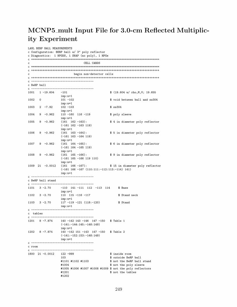
MCNP5 mult Input File for 3.0-cm Reflected Multiplic-
ity ExperimentLANL BERP BALL MEASUREMENTS
c Configuration: BERP ball w/ 3" poly reflector
c Diagnostics: 1 NPODS, 1 SNAP (no poly), 1 HPGe
c ==============================================================================
c CELL CARDS
c ==============================================================================
c ++++++++++++++++++++++++++++++++++++++++++++++++++++++++++++++++++++++++++++++
c begin non-detector cells
c ++++++++++++++++++++++++++++++++++++++++++++++++++++++++++++++++++++++++++++++
c --------------------------------------
c BeRP ball
c --------------------------------------
1001 1 -19.604 -101 $ (19.604 w/ rho,M,V; 19.655
imp:n=1
1002 0 101 -102 $ void between ball and ss304
imp:n=1
1003 2 -7.92 102 -103 $ ss304
imp:n=1
1004 9 -0.962 110 -160 116 -119 $ poly sleeve
imp:n=1
1005 9 -0.962 (161 162 -163): $ 4 in diameter poly reflector
(-161 162 -163 119)
imp:n=1
1006 9 -0.962 (161 163 -164): $ 5 in diameter poly reflector
(-161 163 -164 119)
imp:n=1
1007 9 -0.962 (161 164 -165): $ 6 in diameter poly reflector
(-161 164 -165 119)
imp:n=1
1008 9 -0.962 (161 165 -166): $ 9 in diameter poly reflector
(-161 165 -166 119 110)
imp:n=1
1009 21 -0.0012 (161 166 -167): $ 15 in diameter poly reflector
(-161 166 -167 (110:111:-112:113:-114) 141)
imp:n=1
c --------------------------------------
c BeRP ball stand
c --------------------------------------
1101 3 -2.70 -110 141 -111 112 -113 114 $ Base
imp:n=1
1102 3 -2.70 110 115 -116 -117 $ Stand neck
imp:n=1
1103 3 -2.70 117 -119 -121 (118:-120) $ Stand
imp:n=1
c --------------------------------------
c tables
c --------------------------------------
1201 8 -7.874 140 -142 143 -146 147 -150 $ Table 1
(-141:-144:145:-148:149)
imp:n=1
1202 8 -7.874 140 -142 151 -143 147 -150 $ Table 2
(-141:-152:153:-148:149)
imp:n=1
c --------------------------------------
c room
c --------------------------------------
1800 21 -0.0012 122 -999 $ inside room
103 $ outside BeRP ball
#1101 #1102 #1103 $ not the BeRP ball stand
#1004 $ not the poly sleeve
#1005 #1006 #1007 #1008 #1009 $ not the poly reflectors
#1201 $ not the tables
#1202
249
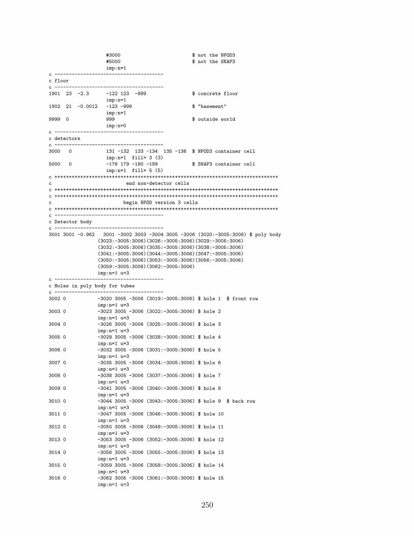
#3000 $ not the NPOD3
#5000 $ not the SNAP3
imp:n=1
c --------------------------------------
c floor
c --------------------------------------
1901 23 -2.3 -122 123 -999 $ concrete floor
imp:n=1
1902 21 -0.0012 -123 -999 $ "basement"
imp:n=1
9999 0 999 $ outside world
imp:n=0
c --------------------------------------
c detectors
c --------------------------------------
3000 0 131 -132 133 -134 135 -136 $ NPOD3 container cell
imp:n=1 fill= 3 (3)
5000 0 -178 179 -180 -199 $ SNAP3 container cell
imp:n=1 fill= 5 (5)
c ++++++++++++++++++++++++++++++++++++++++++++++++++++++++++++++++++++++++++++++
c end non-detector cells
c ++++++++++++++++++++++++++++++++++++++++++++++++++++++++++++++++++++++++++++++
c ++++++++++++++++++++++++++++++++++++++++++++++++++++++++++++++++++++++++++++++
c begin NPOD version 3 cells
c ++++++++++++++++++++++++++++++++++++++++++++++++++++++++++++++++++++++++++++++
c --------------------------------------
c Detector body
c --------------------------------------
3001 3001 -0.962 3001 -3002 3003 -3004 3005 -3006 (3020:-3005:3006) $ poly body
(3023:-3005:3006)(3026:-3005:3006)(3029:-3005:3006)
(3032:-3005:3006)(3035:-3005:3006)(3038:-3005:3006)
(3041:-3005:3006)(3044:-3005:3006)(3047:-3005:3006)
(3050:-3005:3006)(3053:-3005:3006)(3056:-3005:3006)
(3059:-3005:3006)(3062:-3005:3006)
imp:n=1 u=3
c --------------------------------------
c Holes in poly body for tubes
c --------------------------------------
3002 0 -3020 3005 -3006 (3019:-3005:3006) $ hole 1 $ front row
imp:n=1 u=3
3003 0 -3023 3005 -3006 (3022:-3005:3006) $ hole 2
imp:n=1 u=3
3004 0 -3026 3005 -3006 (3025:-3005:3006) $ hole 3
imp:n=1 u=3
3005 0 -3029 3005 -3006 (3028:-3005:3006) $ hole 4
imp:n=1 u=3
3006 0 -3032 3005 -3006 (3031:-3005:3006) $ hole 5
imp:n=1 u=3
3007 0 -3035 3005 -3006 (3034:-3005:3006) $ hole 6
imp:n=1 u=3
3008 0 -3038 3005 -3006 (3037:-3005:3006) $ hole 7
imp:n=1 u=3
3009 0 -3041 3005 -3006 (3040:-3005:3006) $ hole 8
imp:n=1 u=3
3010 0 -3044 3005 -3006 (3043:-3005:3006) $ hole 9 $ back row
imp:n=1 u=3
3011 0 -3047 3005 -3006 (3046:-3005:3006) $ hole 10
imp:n=1 u=3
3012 0 -3050 3005 -3006 (3049:-3005:3006) $ hole 11
imp:n=1 u=3
3013 0 -3053 3005 -3006 (3052:-3005:3006) $ hole 12
imp:n=1 u=3
3014 0 -3056 3005 -3006 (3055:-3005:3006) $ hole 13
imp:n=1 u=3
3015 0 -3059 3005 -3006 (3058:-3005:3006) $ hole 14
imp:n=1 u=3
3016 0 -3062 3005 -3006 (3061:-3005:3006) $ hole 15
imp:n=1 u=3
250
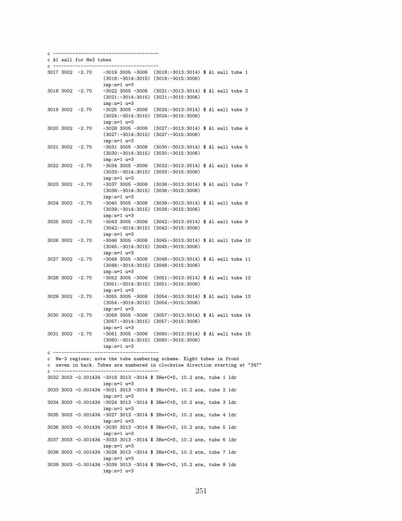
c --------------------------------------
c Al wall for He3 tubes
c --------------------------------------
3017 3002 -2.70 -3019 3005 -3006 (3018:-3013:3014) $ Al wall tube 1
(3018:-3014:3015) (3018:-3015:3006)
imp:n=1 u=3
3018 3002 -2.70 -3022 3005 -3006 (3021:-3013:3014) $ Al wall tube 2
(3021:-3014:3015) (3021:-3015:3006)
imp:n=1 u=3
3019 3002 -2.70 -3025 3005 -3006 (3024:-3013:3014) $ Al wall tube 3
(3024:-3014:3015) (3024:-3015:3006)
imp:n=1 u=3
3020 3002 -2.70 -3028 3005 -3006 (3027:-3013:3014) $ Al wall tube 4
(3027:-3014:3015) (3027:-3015:3006)
imp:n=1 u=3
3021 3002 -2.70 -3031 3005 -3006 (3030:-3013:3014) $ Al wall tube 5
(3030:-3014:3015) (3030:-3015:3006)
imp:n=1 u=3
3022 3002 -2.70 -3034 3005 -3006 (3033:-3013:3014) $ Al wall tube 6
(3033:-3014:3015) (3033:-3015:3006)
imp:n=1 u=3
3023 3002 -2.70 -3037 3005 -3006 (3036:-3013:3014) $ Al wall tube 7
(3036:-3014:3015) (3036:-3015:3006)
imp:n=1 u=3
3024 3002 -2.70 -3040 3005 -3006 (3039:-3013:3014) $ Al wall tube 8
(3039:-3014:3015) (3039:-3015:3006)
imp:n=1 u=3
3025 3002 -2.70 -3043 3005 -3006 (3042:-3013:3014) $ Al wall tube 9
(3042:-3014:3015) (3042:-3015:3006)
imp:n=1 u=3
3026 3002 -2.70 -3046 3005 -3006 (3045:-3013:3014) $ Al wall tube 10
(3045:-3014:3015) (3045:-3015:3006)
imp:n=1 u=3
3027 3002 -2.70 -3049 3005 -3006 (3048:-3013:3014) $ Al wall tube 11
(3048:-3014:3015) (3048:-3015:3006)
imp:n=1 u=3
3028 3002 -2.70 -3052 3005 -3006 (3051:-3013:3014) $ Al wall tube 12
(3051:-3014:3015) (3051:-3015:3006)
imp:n=1 u=3
3029 3002 -2.70 -3055 3005 -3006 (3054:-3013:3014) $ Al wall tube 13
(3054:-3014:3015) (3054:-3015:3006)
imp:n=1 u=3
3030 3002 -2.70 -3058 3005 -3006 (3057:-3013:3014) $ Al wall tube 14
(3057:-3014:3015) (3057:-3015:3006)
imp:n=1 u=3
3031 3002 -2.70 -3061 3005 -3006 (3060:-3013:3014) $ Al wall tube 15
(3060:-3014:3015) (3060:-3015:3006)
imp:n=1 u=3
c --------------------------------------
c He-3 regions; note the tube numbering scheme. Eight tubes in front
c seven in back. Tubes are numbered in clockwise direction starting at "347"
c --------------------------------------
3032 3003 -0.001434 -3018 3013 -3014 $ 3He+C+O, 10.2 atm, tube 1 ldr
imp:n=1 u=3
3033 3003 -0.001434 -3021 3013 -3014 $ 3He+C+O, 10.2 atm, tube 2 ldr
imp:n=1 u=3
3034 3003 -0.001434 -3024 3013 -3014 $ 3He+C+O, 10.2 atm, tube 3 ldr
imp:n=1 u=3
3035 3003 -0.001434 -3027 3013 -3014 $ 3He+C+O, 10.2 atm, tube 4 ldr
imp:n=1 u=3
3036 3003 -0.001434 -3030 3013 -3014 $ 3He+C+O, 10.2 atm, tube 5 ldr
imp:n=1 u=3
3037 3003 -0.001434 -3033 3013 -3014 $ 3He+C+O, 10.2 atm, tube 6 ldr
imp:n=1 u=3
3038 3003 -0.001434 -3036 3013 -3014 $ 3He+C+O, 10.2 atm, tube 7 ldr
imp:n=1 u=3
3039 3003 -0.001434 -3039 3013 -3014 $ 3He+C+O, 10.2 atm, tube 8 ldr
imp:n=1 u=3
251
3040 3003 -0.001434 -3042 3013 -3014 $ 3He+C+O, 10.2 atm, tube 9 ldr
imp:n=1 u=3
3041 3003 -0.001434 -3045 3013 -3014 $ 3He+C+O, 10.2 atm, tube 10 ldr
imp:n=1 u=3
3042 3003 -0.001434 -3048 3013 -3014 $ 3He+C+O, 10.2 atm, tube 11 ldr
imp:n=1 u=3
3043 3003 -0.001434 -3051 3013 -3014 $ 3He+C+O, 10.2 atm, tube 12 ldr
imp:n=1 u=3
3044 3003 -0.001434 -3054 3013 -3014 $ 3He+C+O, 10.2 atm, tube 13 ldr
imp:n=1 u=3
3045 3003 -0.001434 -3057 3013 -3014 $ 3He+C+O, 10.2 atm, tube 14 ldr
imp:n=1 u=3
3046 3003 -0.001434 -3060 3013 -3014 $ 3He+C+O, 10.2 atm, tube 15 ldr
imp:n=1 u=3
c
3047 3003 -0.001434 -3018 3014 -3015 $ 3He+C+O, 10.2 atm, tube 1 ar
imp:n=1 u=3
3048 3003 -0.001434 -3021 3014 -3015 $ 3He+C+O, 10.2 atm, tube 2 ar
imp:n=1 u=3
3049 3003 -0.001434 -3024 3014 -3015 $ 3He+C+O, 10.2 atm, tube 3 ar
imp:n=1 u=3
3050 3003 -0.001434 -3027 3014 -3015 $ 3He+C+O, 10.2 atm, tube 4 ar
imp:n=1 u=3
3051 3003 -0.001434 -3030 3014 -3015 $ 3He+C+O, 10.2 atm, tube 5 ar
imp:n=1 u=3
3052 3003 -0.001434 -3033 3014 -3015 $ 3He+C+O, 10.2 atm, tube 6 ar
imp:n=1 u=3
3053 3003 -0.001434 -3036 3014 -3015 $ 3He+C+O, 10.2 atm, tube 7 ar
imp:n=1 u=3
3054 3003 -0.001434 -3039 3014 -3015 $ 3He+C+O, 10.2 atm, tube 8 ar
imp:n=1 u=3
3055 3003 -0.001434 -3042 3014 -3015 $ 3He+C+O, 10.2 atm, tube 9 ar
imp:n=1 u=3
3056 3003 -0.001434 -3045 3014 -3015 $ 3He+C+O, 10.2 atm, tube 10 ar
imp:n=1 u=3
3057 3003 -0.001434 -3048 3014 -3015 $ 3He+C+O, 10.2 atm, tube 11 ar
imp:n=1 u=3
3058 3003 -0.001434 -3051 3014 -3015 $ 3He+C+O, 10.2 atm, tube 12 ar
imp:n=1 u=3
3059 3003 -0.001434 -3054 3014 -3015 $ 3He+C+O, 10.2 atm, tube 13 ar
imp:n=1 u=3
3060 3003 -0.001434 -3057 3014 -3015 $ 3He+C+O, 10.2 atm, tube 14 ar
imp:n=1 u=3
3061 3003 -0.001434 -3060 3014 -3015 $ 3He+C+O, 10.2 atm, tube 15 ar
imp:n=1 u=3
c
3062 3003 -0.001434 -3018 3015 -3006 $ 3He+C+O, 10.2 atm, tube 1 udr
imp:n=1 u=3
3063 3003 -0.001434 -3021 3015 -3006 $ 3He+C+O, 10.2 atm, tube 2 udr
imp:n=1 u=3
3064 3003 -0.001434 -3024 3015 -3006 $ 3He+C+O, 10.2 atm, tube 3 udr
imp:n=1 u=3
3065 3003 -0.001434 -3027 3015 -3006 $ 3He+C+O, 10.2 atm, tube 4 udr
imp:n=1 u=3
3066 3003 -0.001434 -3030 3015 -3006 $ 3He+C+O, 10.2 atm, tube 5 udr
imp:n=1 u=3
3067 3003 -0.001434 -3033 3015 -3006 $ 3He+C+O, 10.2 atm, tube 6 udr
imp:n=1 u=3
3068 3003 -0.001434 -3036 3015 -3006 $ 3He+C+O, 10.2 atm, tube 7 udr
imp:n=1 u=3
3069 3003 -0.001434 -3039 3015 -3006 $ 3He+C+O, 10.2 atm, tube 8 udr
imp:n=1 u=3
3070 3003 -0.001434 -3042 3015 -3006 $ 3He+C+O, 10.2 atm, tube 9 udr
imp:n=1 u=3
3071 3003 -0.001434 -3045 3015 -3006 $ 3He+C+O, 10.2 atm, tube 10 udr
imp:n=1 u=3
3072 3003 -0.001434 -3048 3015 -3006 $ 3He+C+O, 10.2 atm, tube 11 udr
imp:n=1 u=3
252
3073 3003 -0.001434 -3051 3015 -3006 $ 3He+C+O, 10.2 atm, tube 12 udr
imp:n=1 u=3
3074 3003 -0.001434 -3054 3015 -3006 $ 3He+C+O, 10.2 atm, tube 13 udr
imp:n=1 u=3
3075 3003 -0.001434 -3057 3015 -3006 $ 3He+C+O, 10.2 atm, tube 14 udr
imp:n=1 u=3
3076 3003 -0.001434 -3060 3015 -3006 $ 3He+C+O, 10.2 atm, tube 15 udr
imp:n=1 u=3
c --------------------------------------
c Cadmium Wrap
c --------------------------------------
3077 3004 -8.65 3007 -3008 3009 -3010 3011 -3005 $ bottom Cd
imp:n=1 u=3
3078 3004 -8.65 3007 -3001 3009 -3010 3005 -3006 $ Cd -x
imp:n=1 u=3
3079 3004 -8.65 3002 -3008 3009 -3010 3005 -3006 $ Cd +x
imp:n=1 u=3
3080 3004 -8.65 3001 -3002 3009 -3003 3005 -3006 $ Cd -y
imp:n=1 u=3
3081 3004 -8.65 3001 -3002 3004 -3010 3005 -3006 $ Cd +y
imp:n=1 u=3
c --------------------------------------
c Cadmium shield
c --------------------------------------
3082 3004 -8.65 3007 -3008 3009 -3010 3006 -3012 $ Cd top
imp:n=1 u=3
c --------------------------------------
c Pre-amp housing
c --------------------------------------
3083 3002 -2.7 3063 -3064 3065 -3066 3012 -3067
imp:n=1 u=3
3084 0 3069 -3070 3071 -3072 3067 -3068 $ inside housing
(-3073:3074:-3075:3076:-3077:3078)
(-3073:3074:-3075:3076:-3079:3080)
imp:n=1 u=3
3085 3002 -2.7 3063 -3064 3065 -3066 3067 -3068
(-3069:3070:-3071:3072:-3067:3068)
imp:n=1 u=3
3086 3004 -8.65 3073 -3074 3075 -3076 3077 -3078 $ rf shield
imp:n=1 u=3
3087 3006 -2.33 3073 -3074 3075 -3076 3079 -3080 $ dielectric circuit board
imp:n=1 u=3
c --------------------------------------
c Display Housing
c --------------------------------------
3088 0 3001 -3002 3009 -3081 3068 -3082
(-3001:3083:-3009:3081:-3068:3082)
(-3083:3084:-3009:3085:-3068:3082)
(-3084:3002:-3009:3081:-3068:3082)
(-3083:3084:-3086:3081:-3068:3082)
(-3083:3084:-3085:3086:-3087:3082)
(-3083:3084:-3085:3086:-3088:3089)
imp:n=1 u=3
3089 3002 -2.7 3001 -3083 3009 -3081 3068 -3082 $ Al wall, -x
imp:n=1 u=3
3090 3002 -2.7 3083 -3084 3009 -3085 3068 -3082 $ Al wall, -y
imp:n=1 u=3
3091 3002 -2.7 3084 -3002 3009 -3081 3068 -3082 $ Al wall, +x
imp:n=1 u=3
3092 3002 -2.7 3083 -3084 3086 -3081 3068 -3082 $ Al wall, +y
imp:n=1 u=3
3093 3002 -2.7 3083 -3084 3085 -3086 3087 -3082 $ Al top
imp:n=1 u=3
3094 3006 -2.33 3083 -3084 3085 -3086 3088 -3089 $ dielectric circuit board
imp:n=1 u=3
c
3999 0 (-3001:3002:-3003:3004:-3005:3006) $ outside detector
(-3007:3008:-3009:3010:-3011:3005) $ for use in universes
253
(-3007:3001:-3009:3010:-3005:3006)
(-3002:3008:-3009:3010:-3005:3006)
(-3001:3002:-3009:3003:-3005:3006)
(-3001:3002:-3004:3010:-3005:3006)
(-3007:3008:-3009:3010:-3006:3012)
(-3063:3064:-3065:3066:-3012:3067)
(-3063:3064:-3065:3066:-3067:3068)
(-3001:3002:-3009:3081:-3068:3082)
imp:n=1 u=3
c ++++++++++++++++++++++++++++++++++++++++++++++++++++++++++++++++++++++++++++++
c end NPOD version 3 cells
c ++++++++++++++++++++++++++++++++++++++++++++++++++++++++++++++++++++++++++++++
c ++++++++++++++++++++++++++++++++++++++++++++++++++++++++++++++++++++++++++++++
c begin SNAP3 cells
c ++++++++++++++++++++++++++++++++++++++++++++++++++++++++++++++++++++++++++++++
c --------------------------------------
c Tripod plate
c --------------------------------------
5001 5001 -2.7 5002 -5003 -5004 -5005 $ Aluminum
imp:n=1 u=5
c
c --------------------------------------
c Bottom cover
c --------------------------------------
5002 5002 -0.962 5003 -5006 -5007 -5008 $ High Density poly
imp:n=1 u=5
c --------------------------------------
c He3 Tube
c --------------------------------------
5003 5003 -0.001284 -5009 5011 -5012 $ lower dead region
imp:n=1 u=5
5004 5003 -0.001284 -5009 5012 -5013 $ active region l = 10.1
imp:n=1 u=5
5005 5003 -0.001284 -5009 5013 -5014 $ upper dead region
imp:n=1 u=5
5006 5001 -2.7 5010 -5015 -5016 (5009:-5011:5014) $ SST wall of he3 tube
imp:n=1 u=5
c --------------------------------------
c HN Connector
c --------------------------------------
5007 0 -5018 5015 -5027
imp:n=1 u=5
5008 5004 -7.89 -5017 5015 -5027 5018
imp:n=1 u=5
5009 5004 -7.89 5027 -5039 5018 -5017
imp:n=1 u=5
5010 5002 -0.962 5026 -5021 5019 -5020 $ poly sleeve
imp:n=1 u=5
5011 5005 -8.65 5021 -5022 5019 -5020 $ Cd top
imp:n=1 u=5
5012 5002 -0.962 5022 -5027 5019 -5020 $ top spacer - pol
imp:n=1 u=5
5013 5005 -8.65 5006 -5023 5024 -5025 $ Cd shield
imp:n=1 u=5
c --------------------------------------
c Detector body
c --------------------------------------
5014 5002 -0.962 5006 -5027 5028 -5007 -5008
(-5046:-5033: 5034)
(-5029: 5030)
5048
imp:n=1 u=5
5015 5002 -0.962 5006 -5027 5028 -5007 -5048
imp:n=1 u=5
c --------------------------------------
c Protective cover
c --------------------------------------
5016 5001 -2.7 5003 -5039 5007 -5032 -5008
254
imp:n=1 u=5
c --------------------------------------
c Inner front protective cover
c --------------------------------------
5017 5001 -2.7 5006 -5027 5033 -5034 5046 -5008
imp:n=1 u=5
c --------------------------------------
c Removable CH2 Shield
c --------------------------------------
5018 0 5008 -5047 5035 -5036 5003 -5039 $ NO CH2 in front of S
c 5018 5002 -0.962 5008 -5047 5035 -5036 5003 -5039 $ CH2 in front of SN
imp:n=1 u=5
c --------------------------------------
c Top cover
c --------------------------------------
5019 5002 -0.962 -5007 -5008 5027 -5039 (5019 (-5038:5037)) $ top plate
imp:n=1 u=5
c --------------------------------------
c MC PCB Housing
c --------------------------------------
5020 0 -5043 -5008 5039 -5044 (5043:5008:-5039:5041)
(5043:5008:-5041:5044) (5042:5040:-5041:5044)
imp:n=1 u=5
5021 5001 -2.7 -5043 -5008 5039 -5041
imp:n=1 u=5
5022 5001 -2.7 -5043 -5008 5041 -5044 (5042:5040:-5041:5044)
imp:n=1 u=5
5023 0 -5042 -5040 5041 -5044
imp:n=1 u=5
c --------------------------------------
c Display housing
c --------------------------------------
5024 5001 -2.7 -5043 -5008 5044 -5045
imp:n=1 u=5
c --------------------------------------
c Cd bottom shield
c --------------------------------------
5025 5005 -8.65 5006 -5026 -5024
imp:n=1 u=5
c --------------------------------------
c voids in detector
c --------------------------------------
5026 0 5010 -5015 5016 -5019
imp:n=1 u=5
5027 0 5015 -5027 5017 -5019
imp:n=1 u=5
5028 0 5023 -5027 5020 -5028
imp:n=1 u=5
5029 0 5026 -5023 5020 -5024
imp:n=1 u=5
5030 0 5006 -5023 5025 -5028
imp:n=1 u=5
5031 0 5026 -5010 -5019
imp:n=1 u=5
5032 0 5006 -5027 5029 -5030 5028 -5046 5048
imp:n=1 u=5
5033 0 5027 -5039 -5037 (5038:-5019) 5017
imp:n=1 u=5
5034 0 5027 -5039 -5018
imp:n=1 u=5
c --------------------------------------
c voids outside detector
c --------------------------------------
5035 0 5001 -5002 -5031
imp:n=1 u=5
5036 0 5002 -5003 5004 -5031
imp:n=1 u=5
5037 0 5002 -5003 5005 -5031 -5004
255
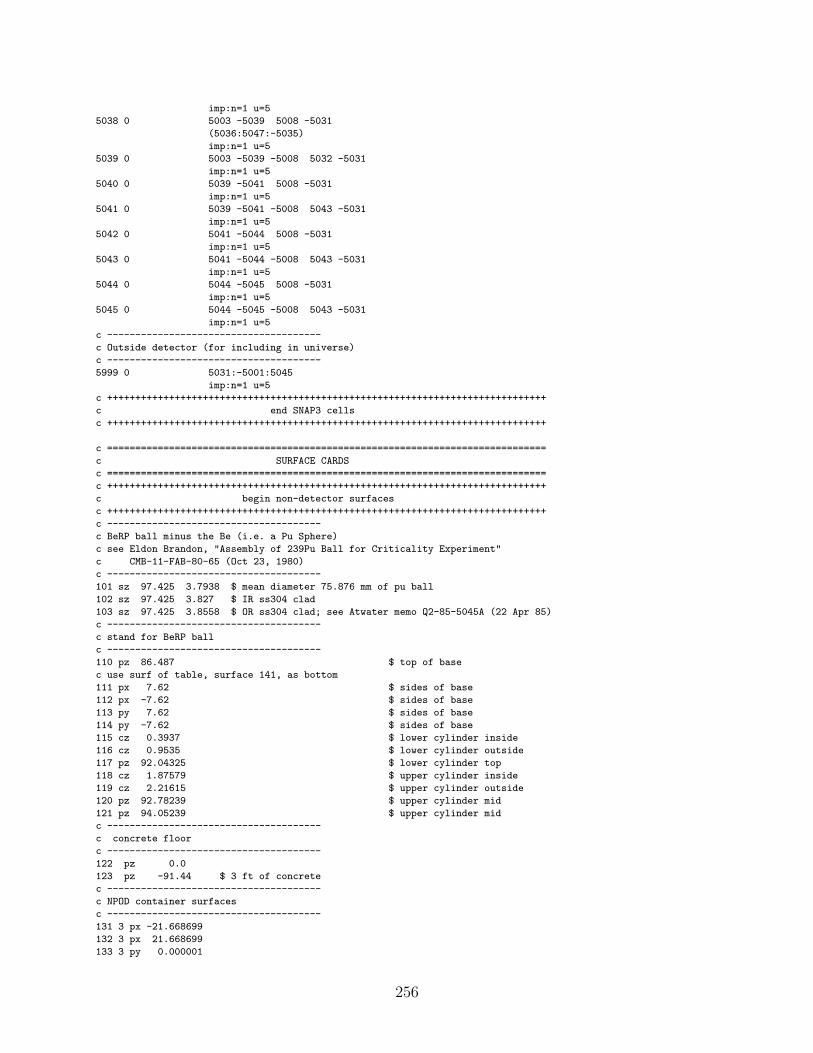
imp:n=1 u=5
5038 0 5003 -5039 5008 -5031
(5036:5047:-5035)
imp:n=1 u=5
5039 0 5003 -5039 -5008 5032 -5031
imp:n=1 u=5
5040 0 5039 -5041 5008 -5031
imp:n=1 u=5
5041 0 5039 -5041 -5008 5043 -5031
imp:n=1 u=5
5042 0 5041 -5044 5008 -5031
imp:n=1 u=5
5043 0 5041 -5044 -5008 5043 -5031
imp:n=1 u=5
5044 0 5044 -5045 5008 -5031
imp:n=1 u=5
5045 0 5044 -5045 -5008 5043 -5031
imp:n=1 u=5
c --------------------------------------
c Outside detector (for including in universe)
c --------------------------------------
5999 0 5031:-5001:5045
imp:n=1 u=5
c ++++++++++++++++++++++++++++++++++++++++++++++++++++++++++++++++++++++++++++++
c end SNAP3 cells
c ++++++++++++++++++++++++++++++++++++++++++++++++++++++++++++++++++++++++++++++
c ==============================================================================
c SURFACE CARDS
c ==============================================================================
c ++++++++++++++++++++++++++++++++++++++++++++++++++++++++++++++++++++++++++++++
c begin non-detector surfaces
c ++++++++++++++++++++++++++++++++++++++++++++++++++++++++++++++++++++++++++++++
c --------------------------------------
c BeRP ball minus the Be (i.e. a Pu Sphere)
c see Eldon Brandon, "Assembly of 239Pu Ball for Criticality Experiment"
c CMB-11-FAB-80-65 (Oct 23, 1980)
c --------------------------------------
101 sz 97.425 3.7938 $ mean diameter 75.876 mm of pu ball
102 sz 97.425 3.827 $ IR ss304 clad
103 sz 97.425 3.8558 $ OR ss304 clad; see Atwater memo Q2-85-5045A (22 Apr 85)
c --------------------------------------
c stand for BeRP ball
c --------------------------------------
110 pz 86.487 $ top of base
c use surf of table, surface 141, as bottom
111 px 7.62 $ sides of base
112 px -7.62 $ sides of base
113 py 7.62 $ sides of base
114 py -7.62 $ sides of base
115 cz 0.3937 $ lower cylinder inside
116 cz 0.9535 $ lower cylinder outside
117 pz 92.04325 $ lower cylinder top
118 cz 1.87579 $ upper cylinder inside
119 cz 2.21615 $ upper cylinder outside
120 pz 92.78239 $ upper cylinder mid
121 pz 94.05239 $ upper cylinder mid
c --------------------------------------
c concrete floor
c --------------------------------------
122 pz 0.0
123 pz -91.44 $ 3 ft of concrete
c --------------------------------------
c NPOD container surfaces
c --------------------------------------
131 3 px -21.668699
132 3 px 21.668699
133 3 py 0.000001
256
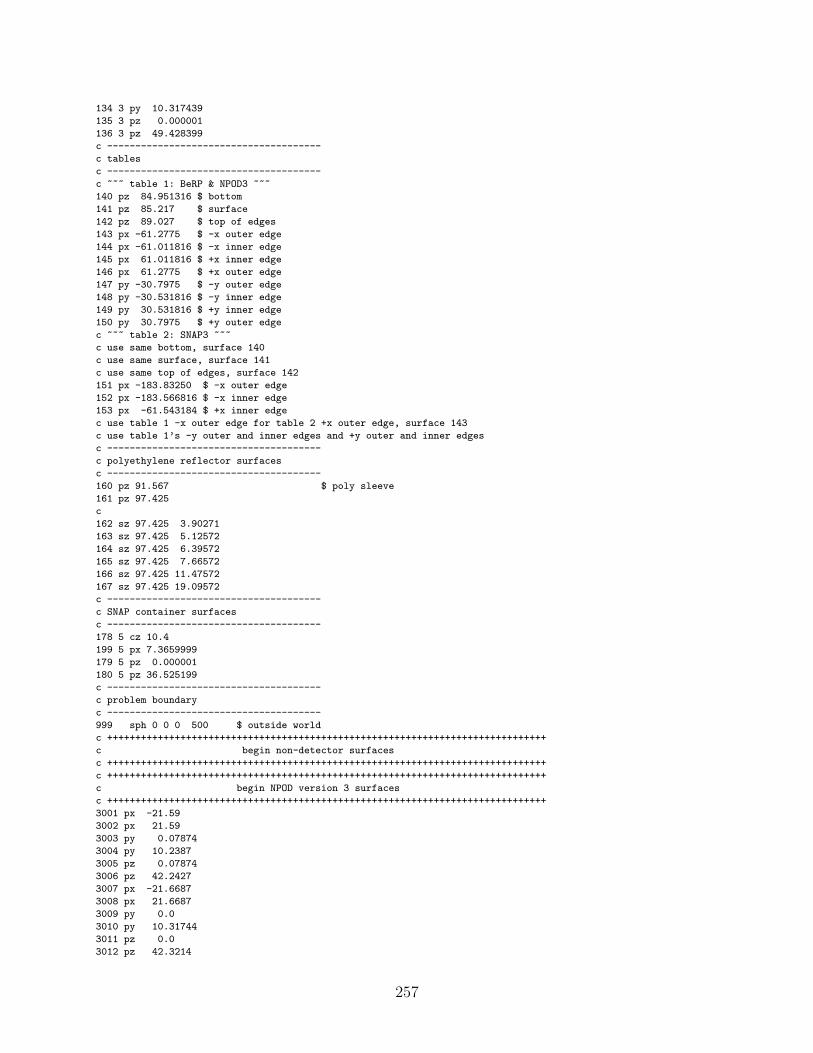
134 3 py 10.317439
135 3 pz 0.000001
136 3 pz 49.428399
c --------------------------------------
c tables
c --------------------------------------
c ~~~ table 1: BeRP & NPOD3 ~~~
140 pz 84.951316 $ bottom
141 pz 85.217 $ surface
142 pz 89.027 $ top of edges
143 px -61.2775 $ -x outer edge
144 px -61.011816 $ -x inner edge
145 px 61.011816 $ +x inner edge
146 px 61.2775 $ +x outer edge
147 py -30.7975 $ -y outer edge
148 py -30.531816 $ -y inner edge
149 py 30.531816 $ +y inner edge
150 py 30.7975 $ +y outer edge
c ~~~ table 2: SNAP3 ~~~
c use same bottom, surface 140
c use same surface, surface 141
c use same top of edges, surface 142
151 px -183.83250 $ -x outer edge
152 px -183.566816 $ -x inner edge
153 px -61.543184 $ +x inner edge
c use table 1 -x outer edge for table 2 +x outer edge, surface 143
c use table 1’s -y outer and inner edges and +y outer and inner edges
c --------------------------------------
c polyethylene reflector surfaces
c --------------------------------------
160 pz 91.567 $ poly sleeve
161 pz 97.425
c
162 sz 97.425 3.90271
163 sz 97.425 5.12572
164 sz 97.425 6.39572
165 sz 97.425 7.66572
166 sz 97.425 11.47572
167 sz 97.425 19.09572
c --------------------------------------
c SNAP container surfaces
c --------------------------------------
178 5 cz 10.4
199 5 px 7.3659999
179 5 pz 0.000001
180 5 pz 36.525199
c --------------------------------------
c problem boundary
c --------------------------------------
999 sph 0 0 0 500 $ outside world
c ++++++++++++++++++++++++++++++++++++++++++++++++++++++++++++++++++++++++++++++
c begin non-detector surfaces
c ++++++++++++++++++++++++++++++++++++++++++++++++++++++++++++++++++++++++++++++
c ++++++++++++++++++++++++++++++++++++++++++++++++++++++++++++++++++++++++++++++
c begin NPOD version 3 surfaces
c ++++++++++++++++++++++++++++++++++++++++++++++++++++++++++++++++++++++++++++++
3001 px -21.59
3002 px 21.59
3003 py 0.07874
3004 py 10.2387
3005 pz 0.07874
3006 pz 42.2427
3007 px -21.6687
3008 px 21.6687
3009 py 0.0
3010 py 10.31744
3011 pz 0.0
3012 pz 42.3214
257
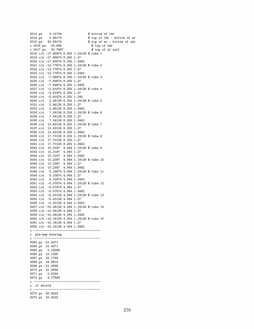
3013 pz 0.15748 $ bottom of ldr
3014 pz 2.49174 $ top of ldr - bottom of ar
3015 pz 40.59174 $ top of ar - bottom of udr
c 3016 pz 43.688 $ top of udr
c 3017 pz 43.7667 $ top of al wall
3018 c/z -17.85874 8.255 1.19126 $ tube 1
3019 c/z -17.85874 8.255 1.27
3020 c/z -17.85874 8.255 1.3462
3021 c/z -12.77874 8.255 1.19126 $ tube 2
3022 c/z -12.77874 8.255 1.27
3023 c/z -12.77874 8.255 1.3462
3024 c/z -7.69874 8.255 1.19126 $ tube 3
3025 c/z -7.69874 8.255 1.27
3026 c/z -7.69874 8.255 1.3462
3027 c/z -2.61874 8.255 1.19126 $ tube 4
3028 c/z -2.61874 8.255 1.27
3029 c/z -2.61874 8.255 1.346
3030 c/z 2.46126 8.255 1.19126 $ tube 5
3031 c/z 2.46126 8.255 1.27
3032 c/z 2.46126 8.255 1.3462
3033 c/z 7.54126 8.255 1.19126 $ tube 6
3034 c/z 7.54126 8.255 1.27
3035 c/z 7.54126 8.255 1.3462
3036 c/z 12.62126 8.255 1.19126 $ tube 7
3037 c/z 12.62126 8.255 1.27
3038 c/z 12.62126 8.255 1.3462
3039 c/z 17.70126 8.255 1.19126 $ tube 8
3040 c/z 17.70126 8.255 1.27
3041 c/z 17.70126 8.255 1.3462
3042 c/z 15.3187 4.064 1.19126 $ tube 9
3043 c/z 15.3187 4.064 1.27
3044 c/z 15.3187 4.064 1.3462
3045 c/z 10.2387 4.064 1.19126 $ tube 10
3046 c/z 10.2387 4.064 1.27
3047 c/z 10.2387 4.064 1.3462
3048 c/z 5.15874 4.064 1.19126 $ tube 11
3049 c/z 5.15874 4.064 1.27
3050 c/z 5.15874 4.064 1.3462
3051 c/z -0.07874 4.064 1.19126 $ tube 12
3052 c/z -0.07874 4.064 1.27
3053 c/z -0.07874 4.064 1.3462
3054 c/z -5.00126 4.064 1.19126 $ tube 13
3055 c/z -5.00126 4.064 1.27
3056 c/z -5.00126 4.064 1.3462
3057 c/z -10.08126 4.064 1.19126 $ tube 14
3058 c/z -10.08126 4.064 1.27
3059 c/z -10.08126 4.064 1.3462
3060 c/z -15.16126 4.064 1.19126 $ tube 15
3061 c/z -15.16126 4.064 1.27
3062 c/z -15.16126 4.064 1.3462
c --------------------------------------
c pre-amp housing
c --------------------------------------
3063 px -21.4071
3064 px 21.4071
3065 py 0.18288
3066 py 10.1295
3067 pz 42.7786
3068 pz 44.8614
3069 px -21.0566
3070 px 21.0566
3071 py 0.5334
3072 py 9.77898
c --------------------------------------
c rf shield
c --------------------------------------
3073 px -20.9423
3074 px 20.9423
258
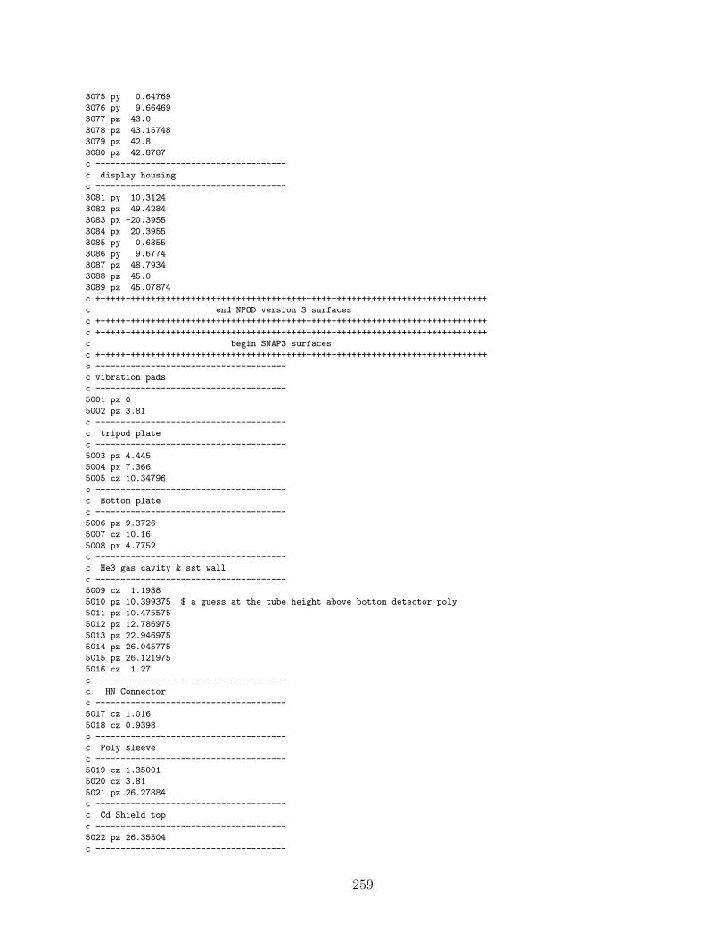
3075 py 0.64769
3076 py 9.66469
3077 pz 43.0
3078 pz 43.15748
3079 pz 42.8
3080 pz 42.8787
c --------------------------------------
c display housing
c --------------------------------------
3081 py 10.3124
3082 pz 49.4284
3083 px -20.3955
3084 px 20.3955
3085 py 0.6355
3086 py 9.6774
3087 pz 48.7934
3088 pz 45.0
3089 pz 45.07874
c ++++++++++++++++++++++++++++++++++++++++++++++++++++++++++++++++++++++++++++++
c end NPOD version 3 surfaces
c ++++++++++++++++++++++++++++++++++++++++++++++++++++++++++++++++++++++++++++++
c ++++++++++++++++++++++++++++++++++++++++++++++++++++++++++++++++++++++++++++++
c begin SNAP3 surfaces
c ++++++++++++++++++++++++++++++++++++++++++++++++++++++++++++++++++++++++++++++
c --------------------------------------
c vibration pads
c --------------------------------------
5001 pz 0
5002 pz 3.81
c --------------------------------------
c tripod plate
c --------------------------------------
5003 pz 4.445
5004 px 7.366
5005 cz 10.34796
c --------------------------------------
c Bottom plate
c --------------------------------------
5006 pz 9.3726
5007 cz 10.16
5008 px 4.7752
c --------------------------------------
c He3 gas cavity & sst wall
c --------------------------------------
5009 cz 1.1938
5010 pz 10.399375 $ a guess at the tube height above bottom detector poly
5011 pz 10.475575
5012 pz 12.786975
5013 pz 22.946975
5014 pz 26.045775
5015 pz 26.121975
5016 cz 1.27
c --------------------------------------
c HN Connector
c --------------------------------------
5017 cz 1.016
5018 cz 0.9398
c --------------------------------------
c Poly sleeve
c --------------------------------------
5019 cz 1.35001
5020 cz 3.81
5021 pz 26.27884
c --------------------------------------
c Cd Shield top
c --------------------------------------
5022 pz 26.35504
c --------------------------------------
259
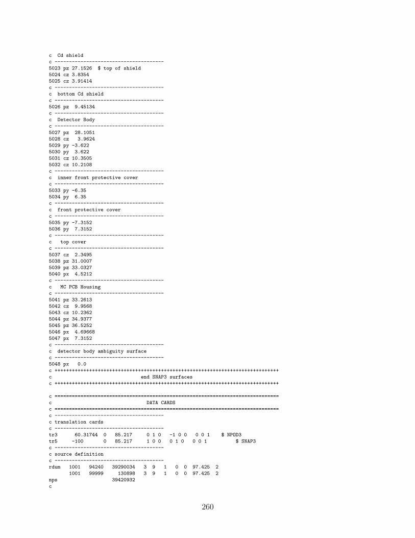
c Cd shield
c --------------------------------------
5023 pz 27.1526 $ top of shield
5024 cz 3.8354
5025 cz 3.91414
c --------------------------------------
c bottom Cd shield
c --------------------------------------
5026 pz 9.45134
c --------------------------------------
c Detector Body
c --------------------------------------
5027 pz 28.1051
5028 cz 3.9624
5029 py -3.622
5030 py 3.622
5031 cz 10.3505
5032 cz 10.2108
c --------------------------------------
c inner front protective cover
c --------------------------------------
5033 py -6.35
5034 py 6.35
c --------------------------------------
c front protective cover
c --------------------------------------
5035 py -7.3152
5036 py 7.3152
c --------------------------------------
c top cover
c --------------------------------------
5037 cz 2.3495
5038 pz 31.0007
5039 pz 33.0327
5040 px 4.5212
c --------------------------------------
c MC PCB Housing
c --------------------------------------
5041 pz 33.2613
5042 cz 9.9568
5043 cz 10.2362
5044 pz 34.9377
5045 pz 36.5252
5046 px 4.69668
5047 px 7.3152
c --------------------------------------
c detector body ambiguity surface
c --------------------------------------
5048 px 0.0
c ++++++++++++++++++++++++++++++++++++++++++++++++++++++++++++++++++++++++++++++
c end SNAP3 surfaces
c ++++++++++++++++++++++++++++++++++++++++++++++++++++++++++++++++++++++++++++++
c ==============================================================================
c DATA CARDS
c ==============================================================================
c --------------------------------------
c translation cards
c --------------------------------------
tr3 60.31744 0 85.217 0 1 0 -1 0 0 0 0 1 $ NPOD3
tr5 -100 0 85.217 1 0 0 0 1 0 0 0 1 $ SNAP3
c --------------------------------------
c source definition
c --------------------------------------
rdum 1001 94240 39290034 3 9 1 0 0 97.425 2
1001 99999 130898 3 9 1 0 0 97.425 2
nps 39420932
c
260

si2 0 3.7938
sp2 -21 2
c
sp3 -3 0.799 4.903
c
si9 0 300.0e8
sp9 0 1
c
c --------------------------------------
c tally cards
c --------------------------------------
c leakage tallies
f01:n 101
c01 0 1
fm01 39420932
fq01 c m
f11:n 103
c11 0 1
fm11 39420932
fq11 c m
c Detector Incident Spectra
f21:n 131 132 133 134 135 136
e21 1e-10 49ilog 1e1
c21 0 1
fm21 39420932
f31:n 178 179 180 199
e31 1e-10 49ilog 1e1
c31 0 1
fm31 39420932
c NPOD Tubes 2 ways
f04:n 3047 3048 3049 3050 3051 3052 3053 3054
3055 3056 3057 3058 3059 3060 3061 T
sd04 300 15r
e04 1e-10 49ilog 1e1
fm04 -39420932 3003 -2
t04 300e8 1e33
cf04 1901
fq04 f m
tf04 16 6j 1
c
f14:n 3047 3048 3049 3050 3051 3052 3053 3054
3055 3056 3057 3058 3059 3060 3061 T
sd14 300 15r
e14 1e-10 49ilog 1e1
fm14 39420932
fu14 2003 $ <- list-mode tally
t14 300e8 1e33
cf14 1901
fq14 f u
tf14 16 6j 1
c SNAP
f24:n 5004
sd24 300
e24 1e-10 49ilog 1e1
t24 300e8 1e33
fm24 -39420932 5003 -2
cf24 1901
fq24 f m
tf24 7j 1
c
f34:n 5004
sd34 300
e34 1e-10 49ilog 1e1
t34 300e8 1e33
fu34 2003
fm34 39420932
cf34 1901
fq34 u t
261
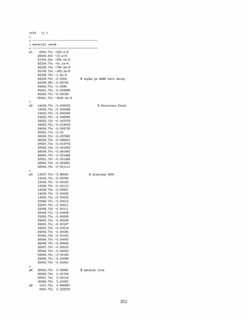
tf34 7j 1
c
c --------------------------------------
c material cards
c --------------------------------------
m1 6000.70c -230.e-6
26000.50c -10.e-6
31000.50c -335.0e-6
92234.70c -41.1e-6
92235.70c -786.6e-6
92236.70c -183.2e-6
92238.70c -1.5e-8
94238.70c -0.0002 $ alpha pu BeRP ball decay
94239.99c -0.93735
94240.70c -0.0595
94241.70c -0.002685
94242.70c -0.00028
95241.70c -2506.0e-6
c
m2 14028.70c -0.009223 $ Stainless Steel
14029.70c -0.000468
14030.70c -0.000309
24050.70c -0.008690
24052.70c -0.167578
24053.70c -0.019002
24054.70c -0.004730
25055.70c -0.02
26054.70c -0.037992
26056.70c -0.596401
26057.70c -0.013774
26058.70c -0.001833
28058.70c -0.081692
28060.70c -0.031468
28061.70c -0.001368
28062.70c -0.004361
28064.70c -0.001111
c
m3 13027.70c -0.96530 $ aluminum 6061
12024.70c -0.00790
12025.70c -0.00100
12026.70c -0.00110
14028.70c -0.00551
14029.70c -0.00029
14030.70c -0.00020
22046.70c -0.00012
22047.70c -0.00011
22048.70c -0.00111
22049.70c -0.00008
22050.70c -0.00008
24050.70c -0.00008
24052.70c -0.00167
24053.70c -0.00019
24054.70c -0.00005
25055.70c -0.00150
26054.70c -0.00040
26056.70c -0.00643
26057.70c -0.00015
26058.70c -0.00002
29063.70c -0.00192
29065.70c -0.00088
30000.70c -0.00250
c
m8 26054.70c 0.05845 $ natural iron
26056.70c 0.91754
26057.70c 0.02119
26058.70c 0.00282
m9 1001.70c 0.666667
6000.70c 0.333333
262
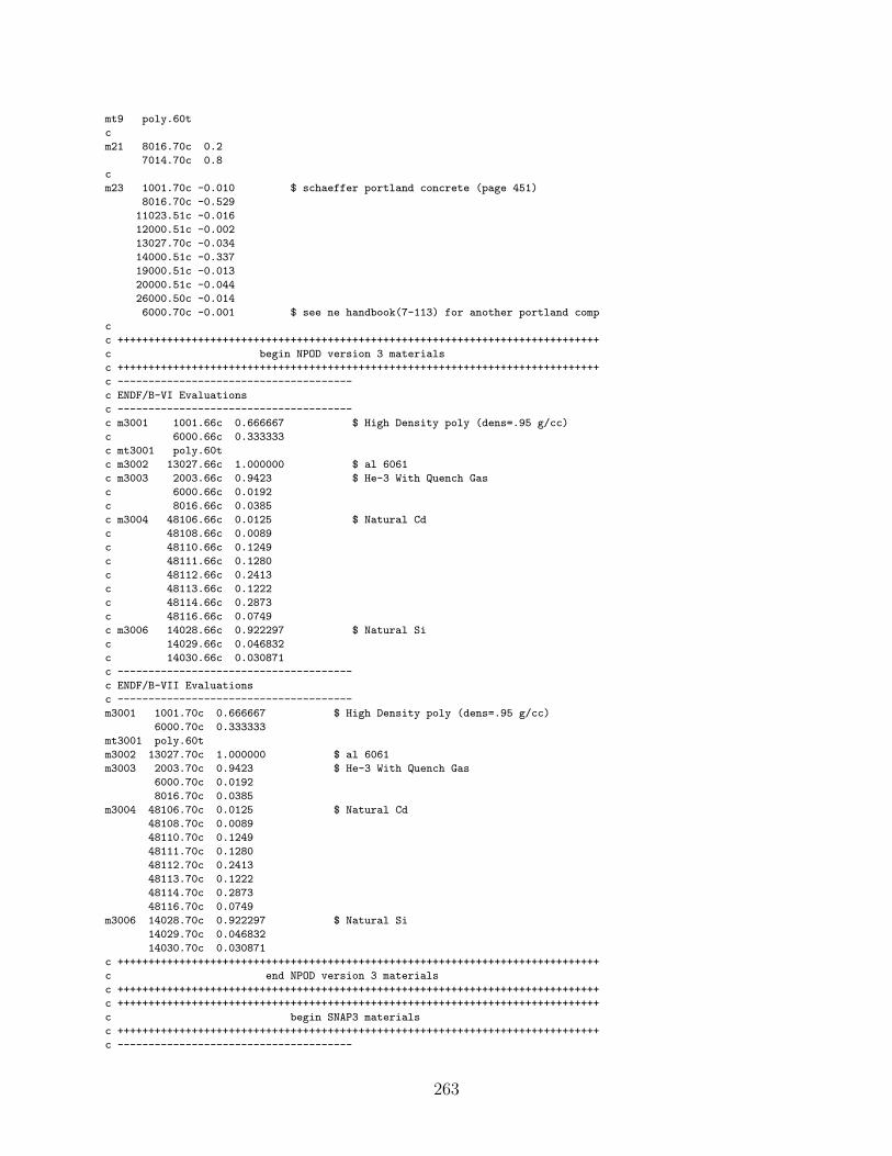
mt9 poly.60t
c
m21 8016.70c 0.2
7014.70c 0.8
c
m23 1001.70c -0.010 $ schaeffer portland concrete (page 451)
8016.70c -0.529
11023.51c -0.016
12000.51c -0.002
13027.70c -0.034
14000.51c -0.337
19000.51c -0.013
20000.51c -0.044
26000.50c -0.014
6000.70c -0.001 $ see ne handbook(7-113) for another portland comp
c
c ++++++++++++++++++++++++++++++++++++++++++++++++++++++++++++++++++++++++++++++
c begin NPOD version 3 materials
c ++++++++++++++++++++++++++++++++++++++++++++++++++++++++++++++++++++++++++++++
c --------------------------------------
c ENDF/B-VI Evaluations
c --------------------------------------
c m3001 1001.66c 0.666667 $ High Density poly (dens=.95 g/cc)
c 6000.66c 0.333333
c mt3001 poly.60t
c m3002 13027.66c 1.000000 $ al 6061
c m3003 2003.66c 0.9423 $ He-3 With Quench Gas
c 6000.66c 0.0192
c 8016.66c 0.0385
c m3004 48106.66c 0.0125 $ Natural Cd
c 48108.66c 0.0089
c 48110.66c 0.1249
c 48111.66c 0.1280
c 48112.66c 0.2413
c 48113.66c 0.1222
c 48114.66c 0.2873
c 48116.66c 0.0749
c m3006 14028.66c 0.922297 $ Natural Si
c 14029.66c 0.046832
c 14030.66c 0.030871
c --------------------------------------
c ENDF/B-VII Evaluations
c --------------------------------------
m3001 1001.70c 0.666667 $ High Density poly (dens=.95 g/cc)
6000.70c 0.333333
mt3001 poly.60t
m3002 13027.70c 1.000000 $ al 6061
m3003 2003.70c 0.9423 $ He-3 With Quench Gas
6000.70c 0.0192
8016.70c 0.0385
m3004 48106.70c 0.0125 $ Natural Cd
48108.70c 0.0089
48110.70c 0.1249
48111.70c 0.1280
48112.70c 0.2413
48113.70c 0.1222
48114.70c 0.2873
48116.70c 0.0749
m3006 14028.70c 0.922297 $ Natural Si
14029.70c 0.046832
14030.70c 0.030871
c ++++++++++++++++++++++++++++++++++++++++++++++++++++++++++++++++++++++++++++++
c end NPOD version 3 materials
c ++++++++++++++++++++++++++++++++++++++++++++++++++++++++++++++++++++++++++++++
c ++++++++++++++++++++++++++++++++++++++++++++++++++++++++++++++++++++++++++++++
c begin SNAP3 materials
c ++++++++++++++++++++++++++++++++++++++++++++++++++++++++++++++++++++++++++++++
c --------------------------------------
263
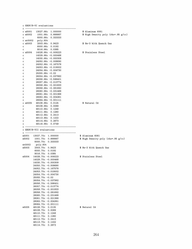
c ENDF/B-VI evaluations
c --------------------------------------
c m5001 13027.66c 1.000000 $ Aluminum 6061
c m5002 1001.66c 0.666667 $ High Density poly (rho=.95 g/cc)
c 6000.66c 0.333333
c mt5002 poly.60t
c m5003 2003.66c 0.9423 $ He-3 With Quench Gas
c 6000.66c 0.0192
c 8016.66c 0.0385
c m5004 14028.66c -0.009223 $ Stainless Steel
c 14029.66c -0.000468
c 14030.66c -0.000309
c 24050.66c -0.008690
c 24052.66c -0.167578
c 24053.66c -0.019002
c 24054.66c -0.004730
c 25055.66c -0.02
c 26054.66c -0.037992
c 26056.66c -0.596401
c 26057.66c -0.013774
c 26058.66c -0.001833
c 28058.66c -0.081692
c 28060.66c -0.031468
c 28061.66c -0.001368
c 28062.66c -0.004361
c 28064.66c -0.001111
c m5005 48106.66c 0.0125 $ Natural Cd
c 48108.66c 0.0089
c 48110.66c 0.1249
c 48111.66c 0.1280
c 48112.66c 0.2413
c 48113.66c 0.1222
c 48114.66c 0.2873
c 48116.66c 0.0749
c --------------------------------------
c ENDF/B-VII evaluations
c --------------------------------------
m5001 13027.70c 1.000000 $ Aluminum 6061
m5002 1001.70c 0.666667 $ High Density poly (rho=.95 g/cc)
6000.70c 0.333333
mt5002 poly.60t
m5003 2003.70c 0.9423 $ He-3 With Quench Gas
6000.70c 0.0192
8016.70c 0.0385
m5004 14028.70c -0.009223 $ Stainless Steel
14029.70c -0.000468
14030.70c -0.000309
24050.70c -0.008690
24052.70c -0.167578
24053.70c -0.019002
24054.70c -0.004730
25055.70c -0.02
26054.70c -0.037992
26056.70c -0.596401
26057.70c -0.013774
26058.70c -0.001833
28058.70c -0.081692
28060.70c -0.031468
28061.70c -0.001368
28062.70c -0.004361
28064.70c -0.001111
m5005 48106.70c 0.0125 $ Natural Cd
48108.70c 0.0089
48110.70c 0.1249
48111.70c 0.1280
48112.70c 0.2413
48113.70c 0.1222
48114.70c 0.2873
264

48116.70c 0.0749
c ++++++++++++++++++++++++++++++++++++++++++++++++++++++++++++++++++++++++++++++
c end SNAP3 materials
c ++++++++++++++++++++++++++++++++++++++++++++++++++++++++++++++++++++++++++++++
c --------------------------------------
c problem specifications
c --------------------------------------
mode n
phys:n 4j 1 $ analog
cut:n 2j 0 $ analog
totnu
prdmp 2j 1
c m0303 is the ACE file for trial 303
XS1 94239.99c 236.998600 m0303 0 1 1 808738 0 0 2.5301E-08 ptable
265
Related Documents