Design of a Chromatic 3D Camera with an End-to-End ... · Design of a chromatic 3D camera with an end-to-end performance model approach P. Trouv´e1 F. Champagnat1 G. Le Besnerais1

Design of a chromatic 3D camera with an end-to-end performance modelapproach

P. Trouve1 F. Champagnat1 G. Le Besnerais1 G. Druart1 J. Idier2

1ONERA-The French Aerospace Lab

F-91761 Palaiseau, France

{pauline.trouve,frederic.champagnat}@onera.fr{guy.le besnerais,guillaume.druart}@onera.fr

2LUNAM Universite, IRCCyN

UMR CNRS 6597 BP 92101

1 rue de la Noe, 44321 Nantes Cedex 3, France

[email protected]

Abstract

In this paper we present a new method for the design ofa 3D single-lens single-frame passive camera. This camerahas a chromatic lens and estimates depth based on a depthfrom defocus technique (DFD). First we develop an originalcalculation of the Cramer Rao Bound to predict the theo-retical camera accuracy. This model takes into account theoptical parameters through the camera Point Spread Func-tion (PSF) and the algorithms parameters applied to theraw image for depth estimation and image restoration. Thismodel is then used for the end-to-end design of a chromaticcamera, dedicated to a small UAV, that is realized and ex-perimentally validated.

1. Introduction

The increasing interest for 3D camera has led to the de-velopment of several depth measure techniques. For in-stance, cheap active cameras such as Kinect [7] are nowavailable. They estimate depth using a projected pattern butare sensitive to perturbation of this pattern, for instance dueto sunlight. Passive 3D cameras using parallax effects areeither cumbersome, when using two separated cameras asin stereoscopy, or reduce image resolution, in the case ofthe plenoptic camera [16], or reduce signal to noise ratio(SNR) in the case of the color filtered aperture of [1]. Otherpassive solutions use depth from focus (DFF), which relieson estimation of the sharpest image among a set of imagesacquired with varying focus [15], or depth from defocus(DFD), i.e. local estimation of the defocus blur by compar-ing two or more images [17]. Such multiple-frames DFDor DFF cameras require the scene to be static during the ac-quisitions which restricts the field of applications. Thus,although more computationally demanding, single frameDFD methods address a larger field [11, 14, 13, 22]. Yetthese techniques have limitations: they suffer from a dead

zone in the depth of field region where blur is quasi-uniformso that depth can not be estimated and there is an ambiguitybetween depths ahead and behind the in-focus plane, whichyield similar defocus blurs.

In the literature various modifications of the camera op-tics are proposed to overcome these defaults and to improvedepth estimation accuracy with a single frame DFD method.Coded apertures are thoroughly studied in [11, 14, 13].Another approach is to use a lens with spectrally varyingblur using either a chromatic aperture [2], or a chromaticlens with some amount of longitudinal chromatic aberration[8, 21]. The latter approach can avoid depth ambiguity ordead zone, in contrast with all other solutions [11, 14, 13, 2].Besides, the camera light intensity is not reduced as in[1, 11, 14, 13] which leads to a higher SNR. Finally as men-tioned in [9, 5, 21], the use of chromatic aberration tends toreduce the lens dimension.

Figure 1. Principle of a computational 3D camera.

Note that these various optical choices increase depth es-timation accuracy but also usually lead to a degradation ofthe image quality that has to be corrected by a dedicatedprocessing. Thus, as illustrated in figure 1, a computational3D camera will have two main processing blocks, one fordepth estimation and one for image restoration. Besides,such solutions also require to rethink the lens design.

Here we base the lens design on the optimization of atheoretical criterion which accounts for both optic and pro-cessing parameters, an approach referred to as codesign,that is briefly reviewed in the next section.

2013 IEEE Conference on Computer Vision and Pattern Recognition Workshops

978-0-7695-4990-3/13 $26.00 © 2013 IEEE

DOI 10.1109/CVPRW.2013.140

939

2013 IEEE Conference on Computer Vision and Pattern Recognition Workshops

978-0-7695-4990-3/13 $26.00 © 2013 IEEE

DOI 10.1109/CVPRW.2013.140

947

2013 IEEE Conference on Computer Vision and Pattern Recognition Workshops

978-0-7695-4990-3/13 $26.00 © 2013 IEEE

DOI 10.1109/CVPRW.2013.140

947

2013 IEEE Conference on Computer Vision and Pattern Recognition Workshops

978-0-7695-4990-3/13 $26.00 © 2013 IEEE

DOI 10.1109/CVPRW.2013.140

953

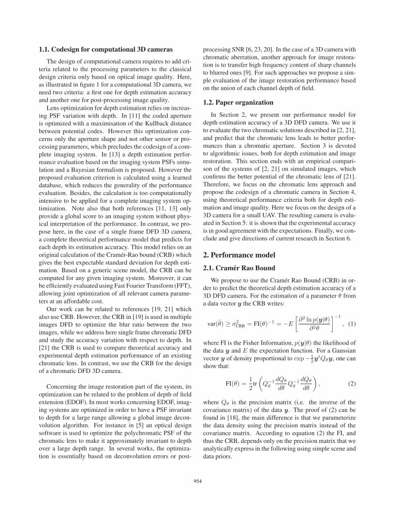
1.1. Codesign for computational 3D cameras

The design of computational camera requires to add cri-teria related to the processing parameters to the classicaldesign criteria only based on optical image quality. Here,as illustrated in figure 1 for a computational 3D camera, weneed two criteria: a first one for depth estimation accuracyand another one for post-processing image quality.

Lens optimization for depth estimation relies on increas-ing PSF variation with depth. In [11] the coded apertureis optimized with a maximisation of the Kullback distancebetween potential codes. However this optimization con-cerns only the aperture shape and not other sensor or pro-cessing parameters, which precludes the codesign of a com-plete imaging system. In [13] a depth estimation perfor-mance evaluation based on the imaging system PSFs simu-lation and a Bayesian formalism is proposed. However theproposed evaluation criterion is calculated using a learneddatabase, which reduces the generality of the performanceevaluation. Besides, the calculation is too computationallyintensive to be applied for a complete imaging system op-timization. Note also that both references [11, 13] onlyprovide a global score to an imaging system without phys-ical interpretation of the performance. In contrast, we pro-pose here, in the case of a single frame DFD 3D camera,a complete theoretical performance model that predicts foreach depth its estimation accuracy. This model relies on anoriginal calculation of the Cramer-Rao bound (CRB) whichgives the best expectable standard deviation for depth esti-mation. Based on a generic scene model, the CRB can becomputed for any given imaging system. Moreover, it canbe efficiently evaluated using Fast Fourier Transform (FFT),allowing joint optimization of all relevant camera parame-ters at an affordable cost.

Our work can be related to references [19, 21] whichalso use CRB. However, the CRB in [19] is used in multipleimages DFD to optimize the blur ratio between the twoimages, while we address here single frame chromatic DFDand study the accuracy variation with respect to depth. In[21] the CRB is used to compare theoretical accuracy andexperimental depth estimation performance of an existingchromatic lens. In contrast, we use the CRB for the designof a chromatic DFD 3D camera.

Concerning the image restoration part of the system, itsoptimization can be related to the problem of depth of fieldextension (EDOF). In most works concerning EDOF, imag-ing systems are optimized in order to have a PSF invariantto depth for a large range allowing a global image decon-volution algorithm. For instance in [5] an optical designsoftware is used to optimize the polychromatic PSF of thechromatic lens to make it approximately invariant to depthover a large depth range. In several works, the optimiza-tion is essentially based on deconvolution errors or post-

processing SNR [6, 23, 20]. In the case of a 3D camera withchromatic aberration, another approach for image restora-tion is to transfer high frequency content of sharp channelsto blurred ones [9]. For such approaches we propose a sim-ple evaluation of the image restoration performance basedon the union of each channel depth of field.

1.2. Paper organization

In Section 2, we present our performance model fordepth estimation accuracy of a 3D DFD camera. We use itto evaluate the two chromatic solutions described in [2, 21],and predict that the chromatic lens leads to better perfor-mances than a chromatic aperture. Section 3 is devotedto algorithmic issues, both for depth estimation and imagerestoration. This section ends with an empirical compari-son of the systems of [2, 21] on simulated images, whichconfirms the better potential of the chromatic lens of [21].Therefore, we focus on the chromatic lens approach andpropose the codesign of a chromatic camera in Section 4,using theoretical performance criteria both for depth esti-mation and image quality. Here we focus on the design of a3D camera for a small UAV. The resulting camera is evalu-ated in Section 5: it is shown that the experimental accuracyis in good agreement with the expectations. Finally, we con-clude and give directions of current research in Section 6.

2. Performance model

2.1. Cramer Rao Bound

We propose to use the Cramer Rao Bound (CRB) in or-der to predict the theoretical depth estimation accuracy of a3D DFD camera. For the estimation of a parameter θ froma data vector y the CRB writes:

var(θ) ≥ σ2CRB = FI(θ)−1 = −E

[∂2 ln p(y|θ)

∂2θ

]−1

, (1)

where FI is the Fisher Information, p(y|θ) the likelihood ofthe data y and E the expectation function. For a Gaussianvector y of density proportional to exp− 1

2ytQθy, one can

show that:

FI(θ) =1

2tr

(Q−1θ

dQθdθ

Q−1θ

dQθdθ

), (2)

where Qθ is the precision matrix (i.e. the inverse of thecovariance matrix) of the data y. The proof of (2) can befound in [18], the main difference is that we parameterizethe data density using the precision matrix instead of thecovariance matrix. According to equation (2) the FI, andthus the CRB, depends only on the precision matrix that weanalytically express in the following using simple scene anddata priors.

940948948954

2.2. Image model

Defocus blur is a spatially varying blur, so an imagepatch is usually modeled with the local convolution of ascene patch with the PSF and addition of random acqui-sition noise. Using the vector representation on image andscene patches we have:

Y = HX +N , (3)

with Y = [ytRytGy

tB]t, X = [xtRx

tGx

tB]t, where for each

channel c, yc (respectively xc) collects pixels of the image(resp. scene) patch in the lexicographical order. N standsfor the noise process which is modeled as a zero mean whiteGaussian noise (WGN) with variance σ2

n. The observationmatrix writes:

H(d) =

⎡⎣ HR(d) 0 0

0 HG(d) 00 0 HB(d)

⎤⎦ . (4)

Each Hc(d) is a convolution matrix which depends on thedefocus PSF of the channel c. As we consider small patches,some care has to be taken concerning boundary hypothe-ses. In particular the usual periodic model associated withFourier approaches is not suited here. In the sequel we use”valid” convolutions where the support of xc is enlargedwith respect to the one of yc according to the PSF support[10, Section 4.3.2]. N is the length of each vectors yc, Mthe length of each vector xc thus each Hc is a convolutionmatrix of size N ×M . Note that the proposed formalismallows to model both 3CCD and color filter array (CFA)sensors. Modeling a CFA sensor just amounts to removeadequate lines from full convolution matrices Hc.

2.3. Scene model

In the context of local PSF estimation, a Gaussian prioron the scene is often very effective as shown for instance in[12, 3, 22]. However as mentioned in [21], when dealingwith chromatic data the components in the RGB decompo-sition are partially correlated. Following [4, 21] we pro-pose to use the luminance (L) and the red-green (C1) andblue-yellow chrominance (C2) decomposition instead of theRGB decomposition using the transform:⎡

⎣ xRxGxB

⎤⎦ = T ⊗ IM,M ,

⎡⎣ xL

xC1

xC2

⎤⎦ (5)

where ⊗ stands for the Kronecker product, IM,M is theidentity matrix of size M ×M and:

T =

⎡⎢⎣

1√3

−1√2

−1√6

1√3

1√2

−1√6

1√3

0 2√6

⎤⎥⎦ . (6)

According to [4], the three components of the lumi-nance/chrominance (LC) decomposition can be assumed tobe uncorrelated. We then use the Gaussian prior:

p(XLC , σ2xC

) ∝ exp

(−‖DCX

LC‖22σ2

xC

)(7)

where XLC = [xtLxtC1

xtC2]t and:

DC =

⎡⎣√μcD 0 00 D 00 0 D

⎤⎦ . (8)

D is the vertical concatenation of the convolution matri-ces relative to the horizontal and vertical first order deriva-tion operator, and μC is the ratio of the luminance and thechrominance variances. As in [4] μc is fixed at 0.05. Thusthe image model becomes:

Y = HC(d)XLC +N (9)

HC(d) = H(d)T ⊗ IM,M . (10)

2.4. Likelihood marginalisation

The data likelihood is then derived through a marginali-sation of the scene [3, 12, 22],

p(Y |d, σ2n, σ

2xC

) = (11)∫p(Y |XLC , d, σ2

n)p(XLC , σ2

xC)dXLC , (12)

which is tractable only for a Gaussian prior on the scene.Replacing (7) into (12) and using a Gaussian density for thenoise process we obtain:

p(Y |θ) =∣∣∣∣Qθ

2π

∣∣∣∣12

+

exp

(−1

2Y tQθY

), (13)

where θ = {d, σ2n, σ

2xc} and |Qθ|+ is the product of the non

zero eigenvalues of Qθ which can be written as:

Qθ =1

σ2n

[I −HC(d)(H

tCHC(d) + αDt

CDC)−1HC(d)

t)].

(14)Parameter α = σ2

n/σ2xC

can be interpreted as the inverse ofa signal to noise ratio. Now by writing Pψ = σ2

nQθ andψ = {d, α} one can evaluate the Fisher Information matrix:

FI(ψ) =1

2tr

(P−1ψ

dPψdψ

P−1ψ

dPψdψ

). (15)

2.5. Computation of the CRB

To simplify the calculation of the CRB, we assume thatthe signal to noise ratio (i.e. α) is known and focus only ondepth estimation. This amounts to assume that ψ = {d}.

941949949955

For each depth d we compute the convolution matricesHR,HG and HB . These PSFs can be simulated either usinga simple Gaussian or pill-box model, or based on Fourieroptics principles or using an optical design software suchas Zemax. Then for a given value of α, we compute thematrice Pψ using (10), (14) and Pψ = σ2

nQθ. To computeFI(d) with (15), we use the numerical differentiation:

dPψdψ

� Pψ+δ − Pψ−δ2δ

, (16)

where δ is a small depth variation with respect to d. Tak-ing the inverse square root of the result gives the theoreticalminimum standard deviation σCRB of Eq. (1).

Note that to reduce calculation time, we decompose Pψwith a Fourier transform and reorganize the frequencies togather together the Fourier components of the three chan-nels at the same frequency. We then deal with a 3× 3 blockdiagonal matrix. Given the imaging system RGB PSFs atdepth (d, d− δ, d+ δ) and a patch size of 21× 21 pixels, avalue of σCRB is obtained in 80ms with a 3GHz processor.

2.6. Comparison of two 3D cameras performances

To illustrate the genericity of the proposed performancemodel, we compare the theoretical accuracy in depth esti-mation of two imaging systems. The first one has a chro-matic lens as in [21] and the other one a chromatic aper-ture as proposed in [2]. The two imaging systems have thesame main focal length, main f-number and detector pixelsize, in order to impose the same optical constraints on bothcamera. We simulate for both cases the PSFs of the threeRGB channels with Gaussian functions whose standard de-viations, normalized with the pixel size, are given by:

σc(d) = ρfcddetpxF#c

(1

fc− 1

d− 1

ddet

), (17)

where fc is the focal length of each channel c, F#c is thef-number of the channel c, ddet is the distance between theoptic and the detector, px the detector pixel size, and ρ is acorrective parameter set to 0.25, so as to fit a Fourier opticsmodel for defocusing.

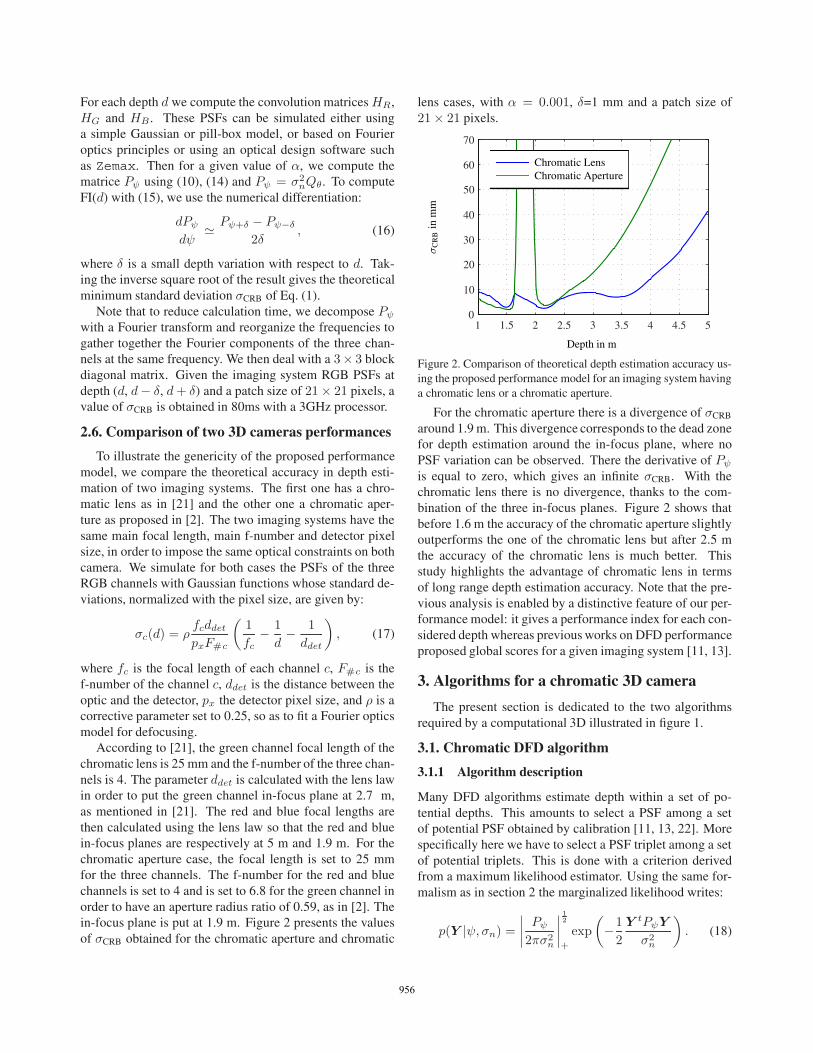
According to [21], the green channel focal length of thechromatic lens is 25 mm and the f-number of the three chan-nels is 4. The parameter ddet is calculated with the lens lawin order to put the green channel in-focus plane at 2.7 m,as mentioned in [21]. The red and blue focal lengths arethen calculated using the lens law so that the red and bluein-focus planes are respectively at 5 m and 1.9 m. For thechromatic aperture case, the focal length is set to 25 mmfor the three channels. The f-number for the red and bluechannels is set to 4 and is set to 6.8 for the green channel inorder to have an aperture radius ratio of 0.59, as in [2]. Thein-focus plane is put at 1.9 m. Figure 2 presents the valuesof σCRB obtained for the chromatic aperture and chromatic

lens cases, with α = 0.001, δ=1 mm and a patch size of21× 21 pixels.

Depth in m

σC

RB

inm

m

Chromatic LensChromatic Aperture

1 1.5 2 2.5 3 3.5 4 4.5 50

10

20

30

40

50

60

70

Figure 2. Comparison of theoretical depth estimation accuracy us-ing the proposed performance model for an imaging system havinga chromatic lens or a chromatic aperture.

For the chromatic aperture there is a divergence of σCRB

around 1.9 m. This divergence corresponds to the dead zonefor depth estimation around the in-focus plane, where noPSF variation can be observed. There the derivative of Pψis equal to zero, which gives an infinite σCRB. With thechromatic lens there is no divergence, thanks to the com-bination of the three in-focus planes. Figure 2 shows thatbefore 1.6 m the accuracy of the chromatic aperture slightlyoutperforms the one of the chromatic lens but after 2.5 mthe accuracy of the chromatic lens is much better. Thisstudy highlights the advantage of chromatic lens in termsof long range depth estimation accuracy. Note that the pre-vious analysis is enabled by a distinctive feature of our per-formance model: it gives a performance index for each con-sidered depth whereas previous works on DFD performanceproposed global scores for a given imaging system [11, 13].

3. Algorithms for a chromatic 3D camera

The present section is dedicated to the two algorithmsrequired by a computational 3D illustrated in figure 1.

3.1. Chromatic DFD algorithm

3.1.1 Algorithm description

Many DFD algorithms estimate depth within a set of po-tential depths. This amounts to select a PSF among a setof potential PSF obtained by calibration [11, 13, 22]. Morespecifically here we have to select a PSF triplet among a setof potential triplets. This is done with a criterion derivedfrom a maximum likelihood estimator. Using the same for-malism as in section 2 the marginalized likelihood writes:

p(Y |ψ, σn) =∣∣∣∣ Pψ2πσ2

n

∣∣∣∣12

+

exp

(−1

2

Y tPψY

σ2n

). (18)

942950950956

3 m

1.4 m1.6 m1.8 m2.2 m

2.4 m2.2 m

2.6 m2.8 m

Raw image Restored image Raw depth mapFigure 3. Example of input and outputs of the codesign 3D camera. Black label is for homogeneous regions insensitive to defocus blur.

This likelihood depends on depth, noise variance, and thescene variance. In order to reduce the number of parame-ters we maximise this likelihood with respect to the noisevariance. This leads to σ2

n = Y tPψY /(N − 3). Replacingσn into equation (18) gives:

p(Y |ψ, σ2n) ∝ |Pψ|

12+ (Y tPψY )−(

3N−32 ).

Maximisation of this generalized likelihood amounts tominimise the criterion:

CGL(ψ) = Y tPψY |Pψ|−1

(3N−3)

+ . (19)

where CGL stands for chromatic generalized likelihood. Ifone writes αk = argminα CGL(dk, α), depth can be esti-mated using the following criterion:

d = argmink

CGL(dk, αk). (20)

Note that this criterion can be seen as a generalization ofthe criterion proposed in [22] to the case of a chromaticlens. In this paper we use the same implementation than theone proposed in [22] based on generalized singular valuedecomposition of the matrices HC and DC .

3.1.2 Empirical chromatic DFD performance

Figure 4. Natural scenes used to simulate image patches.

In this section, we use the previous chromatic DFD algo-rithm on simulated images for the two chromatic imagingsystems: a chromatic aperture and chromatic lens, relatedto [2, 21] described in the section 2.6. For each imagingsystem, we generate 120 image patches of size 21 × 21pixels using scenes patches extracted from natural scenespresented in figure 4. For each depth and each imaging sys-tem the images are obtained with a convolution of scene

Depth 2 m 3 m 4 m 5 mRef. B S B S B S B S[21] 1 1.2 1.3 2.3 0.7 4.1 1.6 12[2] 1.7 2.2 0.3 9.3 0.3 22 4.1 36

Table 1. Bias (B) and standard deviation (S) in cm on depth esti-mation results for two chromatic optical solutions using simulatedimages.

patches with the corresponding Gaussian PSF. White Gaus-sian noise is added to the result with a standard deviationof 0.01, given that the scenes have a normalized intensity.Table 1 shows the bias and the standard deviation of thedepth estimation results. For depths below 3 m the perfor-mances of both imaging systems are quite close, but after3 m the chromatic lens system shows a much better perfor-mance than the chromatic aperture. This is consistent withthe theoretical accuracy comparison made in section 2.6.

3.2. Image restoration

Chromatic aberration induces a inhomogeneous resolu-tion among the RGB channels. Thus, as illustrated in Figure3, the raw RGB image is blurred and requires restorationprocessing. As proposed in [9] a high frequencies trans-fer can be used to improve image resolution. Formally therestored channel is the sum of the original image with aweighted sum of the high frequencies of each channels. In[9], the weights depend on a relative sharpness measure andare set with a calibration step. In our case we simply use thedepth map estimated to determine these weights. Thus wepropose to restore each channel image using:

yi,out = yi,in + ad,RHPR + ad,GHPG + ad,BHPB. (21)

HPc are the high frequencies of the channels c, obtainedwith a high pass filter. The values of ad,c are decreasingfunctions of |d − d0,c| and vary from 0 to 1 where d0 isthe in-focus plane position of the channel c. Figure 3 il-lustrates the resolution gain obtained with such restorationalgorithm and the corresponding depth map obtained withthe chromatic DFD algorithm on a real image acquired withthe camera described in section 4.

943951951957

4. Codesign of a chromatic 3D camera

The performance study conducted in section 2 illustratestheoretically and experimentally the high potential of achromatic lens for depth estimation. Besides, the chromaticlens has no ambiguity around the in-focus plane which en-larges the depth estimation range. Thus we now proceedwith the optimization of a DFD 3D camera with a chromaticlens using our performance model.

4.1. Specifications

Our aim is to design a 3D camera that could be embed-ded on a UAV that is moving in outdoor and indoor condi-tions. For this application we set the depth estimation rangefrom 1 to 5 m with a required depth accuracy of 10 cm. Thisimaging system intends to allow the UAV to reach a point infront of it, so it does not require to have a large field of view.Thus, we restrict the field of view at 25o. Since there is afinite family of existing color sensors, we can hardly contin-uously optimize the sensor parameters. Thus we choose acolor sensor and optimize a chromatic lens for it. The cho-sen color sensor has a pixel size of 3.45μm with a resolutionof 2046× 2452 pixels.

These specifications give us information about the cam-era. Indeed the values of the sensor size and the field of viewlead to a focal length of 25 mm. We choose a f-number of3 in order to have sufficient light intensity to use the cam-era for indoor and outdoor scenes without having too strongoptical design constraints. Besides, we want the UAV toidentify obstacles such as electric wires, posts or scaffolds,thus the depth map spatial X-Y resolution is fixed to approx-imately 2 cm at 3 m. Thus the depth map spatial resolutionis of 160 μm in the image plane. This resolution limits thepatch size to 46 × 46 pixels on the sensor. Since we usea Bayer color sensor it amounts to process patches of size23 × 23 pixels. Yet we need to define the amount of lon-gitudinal chromatic aberration of the lens, characterized bythe RGB in-focus planes positions.

4.2. Design criteria

4.2.1 Depth estimation accuracy

In order to optimize depth estimation for some depth rangewe propose a design criterion named C1 based on the meanvalue of the σCRB in the range L:

C1(L) =< σCRB(d) >d∈L . (22)

4.2.2 Image quality

As chromatic aberration reduces image quality and, as men-tioned in section 3.2, we use a high frequencies transfermethod to improve image resolution. To manage this trans-fer, we need to have at least a sharp channel at each depth.

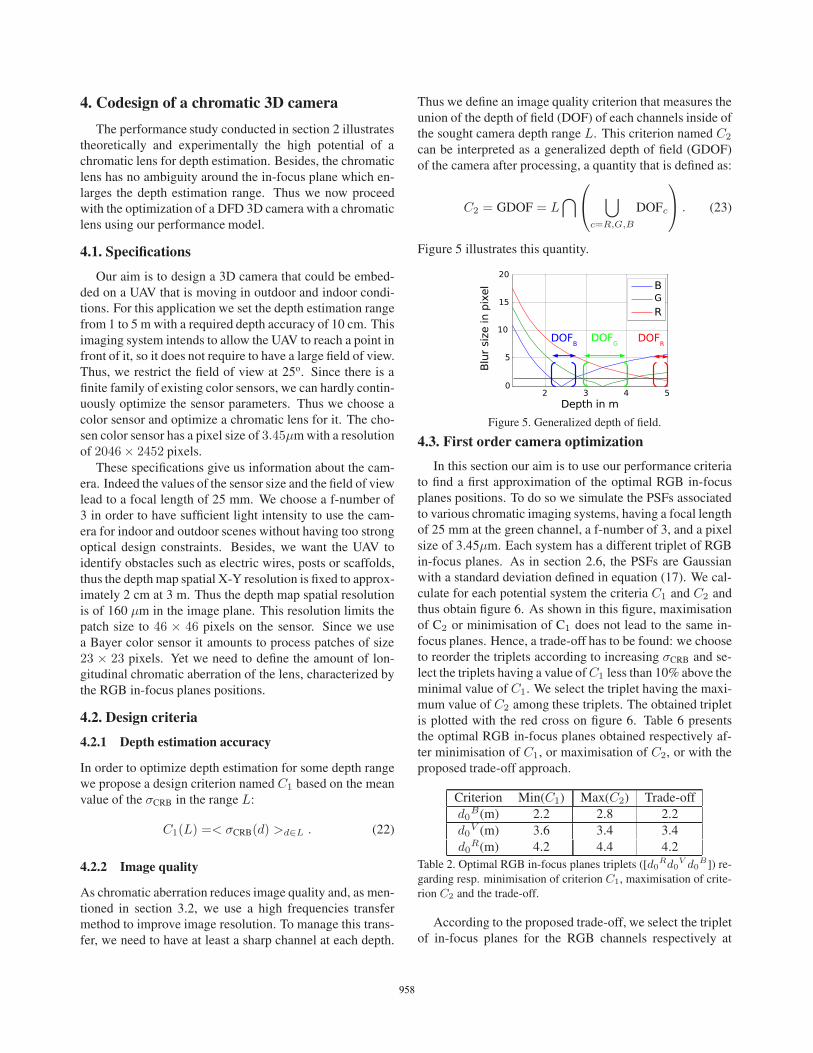
Thus we define an image quality criterion that measures theunion of the depth of field (DOF) of each channels inside ofthe sought camera depth range L. This criterion named C2

can be interpreted as a generalized depth of field (GDOF)of the camera after processing, a quantity that is defined as:

C2 = GDOF = L⋂⎛

⎝ ⋃c=R,G,B

DOFc

⎞⎠ . (23)

Figure 5 illustrates this quantity.

� � � ��

�

��

��

��

��������� �����

�

�

��

�

����������������������������������������

���

���

���

Figure 5. Generalized depth of field.

4.3. First order camera optimization

In this section our aim is to use our performance criteriato find a first approximation of the optimal RGB in-focusplanes positions. To do so we simulate the PSFs associatedto various chromatic imaging systems, having a focal lengthof 25 mm at the green channel, a f-number of 3, and a pixelsize of 3.45μm. Each system has a different triplet of RGBin-focus planes. As in section 2.6, the PSFs are Gaussianwith a standard deviation defined in equation (17). We cal-culate for each potential system the criteria C1 and C2 andthus obtain figure 6. As shown in this figure, maximisationof C2 or minimisation of C1 does not lead to the same in-focus planes. Hence, a trade-off has to be found: we chooseto reorder the triplets according to increasing σCRB and se-lect the triplets having a value ofC1 less than 10% above theminimal value of C1. We select the triplet having the maxi-mum value of C2 among these triplets. The obtained tripletis plotted with the red cross on figure 6. Table 6 presentsthe optimal RGB in-focus planes obtained respectively af-ter minimisation of C1, or maximisation of C2, or with theproposed trade-off approach.

Criterion Min(C1) Max(C2) Trade-offd0B(m) 2.2 2.8 2.2

d0V (m) 3.6 3.4 3.4

d0R(m) 4.2 4.4 4.2

Table 2. Optimal RGB in-focus planes triplets ([d0Rd0V d0B]) re-

garding resp. minimisation of criterion C1, maximisation of crite-rion C2 and the trade-off.

According to the proposed trade-off, we select the tripletof in-focus planes for the RGB channels respectively at

944952952958

Generalized DOF in m (C2)

<σ

CR

B>

inm

m(C

1)

+ Triplet+ Min C1

+ Max C2

+ Trade-off

0 1 2 33

4

5

6

7

Figure 6. Simulated systems scores with respect to C1 and C2.

4.2 m, 3.4 m and 2.2 m. This corresponds to a longitudi-nal chromatic aberration fR − fB around 130 μm.

4.4. Refining the lens optimization

The previews first order optimization gives us the ap-proximate optimal position of the RGB in-focus planes andthe required amount of longitudinal chromatic aberration.According to this constraints, a first architecture is designedusing the optical software Zemax. In contrast to section4.3, we now deal with the real physical lens parameters asfor instance lens curvature radius, thickness or glass type.Starting from this first architecture a more accurate opti-mization of the lens parameters is conducted. In this casewe use jointly the two criteria C1 and C2, evaluated usingthe PSF simulated by Zemax, and the image quality opti-mization algorithms of this software. This leads to a chro-matic lens of longitudinal chromatic aberration of 100μm,with RGB in-focus planes respectively at 3.7, 2.7 and 2.2 m.The resulting lens architecture is shown in figure 7.

� �

�����

60 mm�����

��� �� �� �� �� ��

Figure 7. Architecture of the codesigned lens.

5. Experimental results

We have realized the chromatic lens, according to thespecifications obtained in section 4.4 and evaluate here itsexperimental performance.

(a) (b) (c) (d)

Figure 8. Scenes used as targets in the experiments.

2 m

3 m

4 m

Figure 10. From left to right: RGB image, Kinect and codesignedcamera depth maps. Black label is for homogeneous regions.

5.1. On axis depth estimation accuracy

The PSFs of each channel of the codesigned chromaticlens are calibrated from 1 m to 5 m with a step of 5 cm, witha ground truth given by a telemeter. Acquisitions are madeof colored textured plane scenes put at different distancesfrom the lens. For each scene and at each distance, depth isestimated with the proposed DFD chromatic algorithm onimage patches of size 23 × 23 pixels inside a centred re-gion of size 240× 240 pixels, where the PSF is supposed tobe constant and with a patches overlapping of 50%. Figure8(a) to (d) show four of the scenes used in the experimentand figure 9(a) to (d) show the corresponding mean and thestandard deviation of the depth estimation results with re-spect to the ground truth. Table 3 gives the statistical resultsfor each scene on the full range 1 to 5 m.

Figure 9 (a) (b) (c) (d)Mean bias (absolute value)(cm) 4 4 10 4Mean standard deviation (cm) 7 6 7 6

Table 3. Experimental performances of the codesigned camera.

For each scene, bias is comparable to the PSF calibrationstep (5 cm) and standard deviation is on the order of 7 cm.This results illustrates the good performance of the camerafor depth estimation in the specified depth range.

5.2. Depth map

Figure 10 shows an example of depth map obtained withour camera. Because of the PSF variation with field angle,PSF calibration is carried out off axis for 9 image regionswhere the PSF is assumed to be constant. The depth mapobtained with the chromatic DFD algorithm is compared tothe depth map given by the Kinect. On textured regions,both 3D camera give the same depth levels. In contrast tothe Kinect, which is an active system, we do not estimatedepth on homogeneous regions, because they are insensitiveto defocus. On the other hand, the wire is visible in ourdepth map and does not appear with the Kinect.

945953953959

Depth in m(a)

Dep

thin

m

Depth in m(d)

Dep

thin

m

Depth in m(c)

Dep

thin

m

Depth in m(b)

Dep

thin

m

1.5 2.5 3.5 4.5 5.5 1.5 2.5 3.5 4.5 5.5 1.5 2.5 3.5 4.5 5.51.5 2.5 3.5 4.5 5.5

1.5

2.5

3.5

4.5

5.5

11.5

2.5

3.5

4.5

5.5

1.5

2.5

3.5

4.5

5.5

1.5

2.5

3.5

4.5

5.5

Figure 9. Four on axis depth estimation results resp. for the four targets presented in figure 8. Experimental mean and standard deviationare plotted with error bars (green) with respect to the ground truth given by a telemeter (blue).

6. Conclusion

In this paper we have presented the end-to-end designof a 3D chromatic camera. The accuracy of the depth esti-mation of such a camera is modeled using an original cal-culation of the CRB with generic prior on the scene. Themodel is used to compare a priori two chromatic concepts,namely chromatic lens and chromatic aperture. The modelpredicts a better depth accuracy on a larger range for thechromatic lens concept. This prediction is confirmed by em-pirical evaluation of the depth estimation error statistics fora proposed chromatic DFD estimator on simulated images.

Following the path of the chromatic lens concept, wehave designed a chromatic camera using two criteria: onefor the image quality and another one for depth estimationaccuracy. A prototype of the codesigned camera has beenbuilt and its depth estimation accuracy was empirically as-sessed to around 7 cm from 1 to 5 m range. The proto-type was able to locate fine structures (wires). Note that theproposed approach could be straightforwardly extended todifferent requirements as those used here for a small UAV.Further works involve comparisons of the codesigned chro-matic lens with existing chromatic lens cameras as in [21]and co-operation of a chromatic lens with a coded aperture.

References

[1] Y. Bando, B. Chen, and T. Nishita. Extracting depth andmatte using a color-filtered aperture. ACM TOG, 27(5), 2008.

[2] A. Chakrabarti and T. Zickler. Depth and deblurring from aspectrally varying depth of field. In ECCV, 2012.

[3] A. Chakrabarti, T. Zickler, and W. Freeman. Analyzingspatially-varying blur. In CVPR, 2010.

[4] L. Condat. A generic variational approach for demosaickingfrom an arbitrary color filter array. In ICIP, 2009.

[5] O. Cossairt and S. Nayar. Spectral focal sweep: Extendeddepth of field from chromatic aberrations. In ICCP, 2010.

[6] F. Diaz, F. Goudail, B. Loiseaux, and J. Huignard. Increasein depth of field taking into account deconvolution by opti-mization of pupil mask. Optics Letters, 34(19), 2009.

[7] B. Freedman, A. Shpunt, M. Meir, and A. Yoel. Depthmapping using projected patterns, US patent 20100118123.,2010.

[8] J. Garcia, J. Sanchez, X. Orriols, and X. Binefa. Chromaticaberration and depth extraction. In ICPR, 2000.

[9] F. Guichard, H. Nguyen, R. Tessieres, M. Pyanet, I. Tar-chouna, and F. Cao. Extended depth-of-field using sharpnesstransport across color channels. In Proc. of SPIE, 2009.

[10] J. Idier, editor. Bayesian approach to inverse problems. ISTELtd and John Wiley & Sons Inc, apr. 2008.

[11] A. Levin, R. Fergus, F. Durand, and W. Freeman. Imageand depth from a conventional camera with a coded aperture.ACM TOG, 26(3), 2007.

[12] A. Levin, Y. Weiss, F. Durand, and W. Freeman. Under-standing and evaluating blind deconvolution algorithms. InCVPR, 2009.

[13] M. Martinello and P. Favaro. Single image blind deconvo-lution with higher-order texture statistics. Video Proc. andComp. Video, 2011.

[14] H. Nagahara, C. Zhou, T. Watanabe, H. Ishiguro, and S. Na-yar. Programmable aperture camera using lcos. In ECCV,2010.

[15] H. Nair and C. Stewart. Robust focus ranging. In CVPR,1992.

[16] R. Ng, M. Levoy, M. Bredif, G. Duval, M. Horowitz, andP. Hanrahan. Light field photography with a hand-heldplenoptic camera. Comp. Science Tech. Report, 2005.

[17] A. Pentland. A new sense for depth of field. IEEE Trans. onPAMI, 4, 1987.

[18] B. Porat and B. Friedlander. Computation of the exact infor-mation matrix of gaussian time series with stationary randomcomponents. IEEE Trans. on ASSP, 34(1), 1986.

[19] A. Rajagopalan and S. Chaudhuri. Performance analysis ofmaximum likelihood estimator for recovery of depth fromdefocused images and optimal selection of camera parame-ters. In IJCV, volume 30, 1998.

[20] D. Stork and M. Robinson. Theoretical foundations for jointdigital-optical analysis of electro-optical imaging systems.Applied Optics, 47(10):64–75, 2008.

[21] P. Trouve, F. Champagnat, G. L. Besnerais, G. Druart, andJ. Idier. Chromatic depth from defocus : a theoretical andexperimental performance study. In COSI, 2012.

[22] P. Trouve, F. Champagnat, G. Le Besnerais, and J. Idier. Sin-gle image local blur identification. In ICIP, 2011.

[23] C. Zhou and S. Nayar. What are good apertures for defocusdeblurring? In ICCP, 2009.

946954954960