www.vadosezonejournal.org · Vol. 8, No. 1, February 2009 64 D ٮĥ®½ ãÙÄ«Ý in OWSs are used to distrib- ute septic tank effluent and allow it to infiltrate into the soil. Studies have shown that the wastewater infiltration rate in drainfield trenches declines with time due to the formation of a low-conductivity “biomat” at the soil–trench interface that impedes infiltration and causes ponding in the trench. e for- mation of a mature biomat may take as little as 20 wk (van Cuyk et al., 2001, 2004) or as much as 4 yr (Jenssen and Siegrist, 1991). Onsite wastewater systems can operate effectively in a ponded condition indefinitely but the designed service life of a system should be 20 yr or more (Siegrist, 2007). e biomat is also a zone of intense microbial activity and plays an important role in purifying wastewater. An estimate of the final steady wastewater infiltration rate is needed to evaluate the suitability of soils for installing an OWS and to determine the HLR D . Here, we use this term as one aspect of the long-term acceptance rate (LTAR) for an OWS. e LTAR must also consider the limiting organic loading rate that will result in adequate biological and chemical treatment of pollutants. In this study, we have only addressed hydraulic loading. Siegrist (2007) noted that HLR D values vary widely among states in the United States and are often based on limited empiri- cal evidence. He called for a more rational and uniform approach based on properties of the “soil treatment unit” (STU) and sug- gested using computer models as an aid for designing these systems. Siegrist (2007) recommended using the trench bottom infiltration rate to determine the HLR D and reserving the trench sidewall areas for handling peak flows. How the peak flow capac- ity compares with the HLR D is generally not known. Amoozegar et al. (2007) stressed that soil heterogeneity must be taken into account in estimated HLR D and LTAR values. Computer models of two-dimensional water flow in soils can improve our understanding of OWSs and STUs in a number of ways. ey can quantify processes that we know occur but can’t measure easily (an example is how much flow occurs through trench sidewalls). They can also validate or debunk simple approaches, surprise us with new concepts, identify research gaps, and serve as aides for teaching students and professionals. One such model is HYDRUS-2D, developed by Šimůnek et al. (2006), and it has been used in a number of studies to analyze OWSs (Beach and McCray, 2003; Beal et al., 2008; Bumgarner and McCray, 2007; Finch et al., 2008; Radcliffe et al., 2005; Radcliffe and West, 2007). Heatwole and McCray (2007) used HYDRUS-2D to model infiltration in trenches with simulated, fully developed (mature) biomats in four common soil types and two different OWS architectures (gravel and chamber). ey found that the unsaturated flow properties of the soil played Design Hydraulic Loading Rates for Onsite Wastewater Systems D. E. Radcliffe* and L. T. West Crop and Soil Sciences Dep., Univ. of Georgia, Athens, GA 30602. Received 25 Feb. 2008. *Corresponding author ([email protected]). Vadose Zone J. 8:64–74 doi:10.2136/vzj2008.0045 © Soil Science Society of America 677 S. Segoe Rd. Madison, WI 53711 USA. All rights reserved. No part of this periodical may be reproduced or transmiƩed in any form or by any means, electronic or mechanical, including photocopying, recording, or any informaƟon storage and retrieval system, without permission in wriƟng from the publisher. AÙò®ã®ÊÄÝ: HLR D , design hydraulic loading rate; LTAR, long-term acceptance rate; OWS, onsite wastewater system; STU, soil treat- ment unit. OÙ®¦®Ä½ RÝÙ« Design hydraulic loading rates (HLR D ) are used in specifying the area of the boƩom of drainfield trenches required for onsite wastewater systems (OWSs). Our objecƟve was to develop a method for esƟmaƟng the HLR D based on soil and biomat hydraulic proper Ɵes. We used a two-dimensional computer model to determine the steady flux through the trench boƩom for the 12 USDA soil textural classes with 5 cm of wastewater ponded in the trench as an esƟmate of the performance under normal operaƟng condiƟons. We used two sets of boundary condiƟons at the boƩom of the soil profile: a deep water table and a shallow water table. We also tested how well the simple Bouma equaƟon esƟmated the boƩom flux. To esƟmate the HLR D , we took 50% of the steady trench boƩom flux as a safety factor. Despite the wide range in saturated hydraulic conducƟviƟes of the soil textural classes (8.18–642.98 cm d −1 ), the steady flow through the boƩom of the trench in these soils fell in a narrow range of 2.92 to 10.43 cm d −1 . With a modificaƟon to account for unsaturated flow within the biomat, the Bouma equaƟon produced remarkably accurate esƟmates of trench boƩom flux for all soil textural classes. Based on our esƟmates of HLR D , we divided the soil textural classes into four groups. Our results show that medium-textured soils should have higher HLR D than has been assumed in some systems for esƟmat- ing HLR D due to the importance of unsaturated flow in OWS hydraulic performance.

Welcome message from author
This document is posted to help you gain knowledge. Please leave a comment to let me know what you think about it! Share it to your friends and learn new things together.
Transcript
www.vadosezonejournal.org · Vol. 8, No. 1, February 2009 64
D in OWSs are used to distrib-
ute septic tank effl uent and allow it to infi ltrate into the
soil. Studies have shown that the wastewater infi ltration rate in
drainfi eld trenches declines with time due to the formation of
a low-conductivity “biomat” at the soil–trench interface that
impedes infi ltration and causes ponding in the trench. Th e for-
mation of a mature biomat may take as little as 20 wk (van Cuyk
et al., 2001, 2004) or as much as 4 yr (Jenssen and Siegrist, 1991).
Onsite wastewater systems can operate eff ectively in a ponded
condition indefi nitely but the designed service life of a system
should be 20 yr or more (Siegrist, 2007). Th e biomat is also a
zone of intense microbial activity and plays an important role in
purifying wastewater. An estimate of the fi nal steady wastewater
infi ltration rate is needed to evaluate the suitability of soils for
installing an OWS and to determine the HLRD. Here, we use
this term as one aspect of the long-term acceptance rate (LTAR)
for an OWS. Th e LTAR must also consider the limiting organic
loading rate that will result in adequate biological and chemical
treatment of pollutants. In this study, we have only addressed
hydraulic loading.
Siegrist (2007) noted that HLRD values vary widely among
states in the United States and are often based on limited empiri-
cal evidence. He called for a more rational and uniform approach
based on properties of the “soil treatment unit” (STU) and sug-
gested using computer models as an aid for designing these
systems. Siegrist (2007) recommended using the trench bottom
infi ltration rate to determine the HLRD and reserving the trench
sidewall areas for handling peak fl ows. How the peak fl ow capac-
ity compares with the HLRD is generally not known. Amoozegar
et al. (2007) stressed that soil heterogeneity must be taken into
account in estimated HLRD and LTAR values.
Computer models of two-dimensional water fl ow in soils can
improve our understanding of OWSs and STUs in a number of
ways. Th ey can quantify processes that we know occur but can’t
measure easily (an example is how much fl ow occurs through
trench sidewalls). They can also validate or debunk simple
approaches, surprise us with new concepts, identify research gaps,
and serve as aides for teaching students and professionals.
One such model is HYDRUS-2D, developed by Šimůnek et
al. (2006), and it has been used in a number of studies to analyze
OWSs (Beach and McCray, 2003; Beal et al., 2008; Bumgarner
and McCray, 2007; Finch et al., 2008; Radcliff e et al., 2005;
Radcliff e and West, 2007). Heatwole and McCray (2007) used
HYDRUS-2D to model infi ltration in trenches with simulated,
fully developed (mature) biomats in four common soil types and
two diff erent OWS architectures (gravel and chamber). Th ey
found that the unsaturated fl ow properties of the soil played
Design Hydraulic Loading Rates for Onsite Wastewater SystemsD. E. Radcliff e* and L. T. West
Crop and Soil Sciences Dep., Univ. of Georgia, Athens, GA 30602. Received 25 Feb. 2008. *Corresponding author ([email protected]).
Vadose Zone J. 8:64–74doi:10.2136/vzj2008.0045
© Soil Science Society of America677 S. Segoe Rd. Madison, WI 53711 USA.All rights reserved. No part of this periodical may be reproduced or transmi ed in any form or by any means, electronic or mechanical, including photocopying, recording, or any informa on storage and retrieval system, without permission in wri ng from the publisher.
A : HLRD, design hydraulic loading rate; LTAR, long-term acceptance rate; OWS, onsite wastewater system; STU, soil treat-ment unit.
O R
Design hydraulic loading rates (HLRD) are used in specifying the area of the bo om of drainfi eld trenches required for onsite wastewater systems (OWSs). Our objec ve was to develop a method for es ma ng the HLRD based on soil and biomat hydraulic proper es. We used a two-dimensional computer model to determine the steady fl ux through the trench bo om for the 12 USDA soil textural classes with 5 cm of wastewater ponded in the trench as an es mate of the performance under normal opera ng condi ons. We used two sets of boundary condi ons at the bo om of the soil profi le: a deep water table and a shallow water table. We also tested how well the simple Bouma equa on es mated the bo om fl ux. To es mate the HLRD, we took 50% of the steady trench bo om fl ux as a safety factor. Despite the wide range in saturated hydraulic conduc vi es of the soil textural classes (8.18–642.98 cm d−1), the steady fl ow through the bo om of the trench in these soils fell in a narrow range of 2.92 to 10.43 cm d−1. With a modifi ca on to account for unsaturated fl ow within the biomat, the Bouma equa on produced remarkably accurate es mates of trench bo om fl ux for all soil textural classes. Based on our es mates of HLRD, we divided the soil textural classes into four groups. Our results show that medium-textured soils should have higher HLRD than has been assumed in some systems for es mat-ing HLRD due to the importance of unsaturated fl ow in OWS hydraulic performance.

www.vadosezonejournal.org · Vol. 8, No. 1, February 2009 65
an important role in determining the hydraulic performance
of the systems.
Bouma (1975) developed a simple equation for estimating
steady downward fl ow through the bottom of an OWS trench:
( )− +=0 s b
bs sb
h h ZK K h
Z [1]
where Kbs is the saturated hydraulic conductivity of the biomat
[L T−1], h0 is the height of water ponded in the trench [L], hs
is the pressure head in the soil just beneath the biomat [L], Zb
is the thickness of the biomat [L], and K(hs) is the unsaturated
hydraulic conductivity of the soil [L T−1] at a pressure head of hs.
Under the conditions present in OWS trenches, the fl ux through
the biomat is equal to the fl ux through the underlying soil. Th e
term on the left-hand side of Eq. [1] represents fl ux through
the biomat and the term on the right-hand side represents fl ux
through the underlying soil. Bouma (1975) used a unit hydraulic
gradient below the trench bottom by assuming that the pressure
head would be constant with depth for at least a short interval
beneath the biomat (dh/dz = 0), and hence fl ux would be equal
to the unsaturated hydraulic conductivity of the soil at the soil
water pressure head just beneath the biomat (hs) as shown in Eq.
[1]. To solve Eq. [1] under these conditions, an iterative approach
or a root solver must be used to fi nd the value of hs that will make
the fl uxes on both sides of the equation equal.
Beal et al. (2004a,b) used Eq. [1] to estimate steady fl uxes
through trench bottoms. Th ey showed that for six Australian soils
with saturated hydraulic conductivity (Ks) spanning four orders
of magnitude, the trench bottom fl uxes collapsed to within one
order of magnitude due to the limiting eff ect of the biomat. Th ey
developed a spreadsheet called FLUX (Flux for Septic Trenches)
to solve Eq. [1].
Our overall objective in this study was to develop a method
for estimating the HLRD for OWSs that was fi rmly based on soil
and biomat hydraulic properties. We fi rst used the HYDRUS
simulation model to determine the steady fl ux through the trench
bottom for a wide range of soils with shallow ponding in the
trench. We estimated the steady fl uxes under two sets of boundary
conditions at the bottom of the soil profi le: a deep water table and
a shallow water table. We also tested the eff ect of including soil
heterogeneity. Th en, we tested how well Eq. [1] might estimate
the bottom fl ux. If it were accurate, this method could serve as a
simple alternative to two-dimensional computer models in esti-
mating the bottom fl ux. We also used HYDRUS to determine
the peak fl ow capacity by modeling a trench nearly full of water
and compared the total fl ow out of this system with the total
fl ow under shallow ponding in the trench. Finally, we developed
a method to translate the steady bottom fl ux into a HLRD and
compared it with rates that have been proposed.
Materials and Methods
HYDRUS Simula ons
We used HYDRUS (beta version 7) to model two-dimen-
sional water fl ow in variably saturated soil. Th is new version of
the model is capable of modeling two- and three-dimensional
fl ow, but we used only a two-dimensional analysis. Th e HYDRUS
model is a fi nite-element model that uses a numerical solution to
the Richards (1931) equation. Various equations are available in
the model for describing the soil water retention and unsaturated
hydraulic conductivity functions. We used the van Genuchten
(1980) equation for the water retention curve:
( )( )
θ −θθ = + θ
+ α
s rr
1mn
h
h
[2]
where α [L−1], m (dimensionless), and n (dimensionless) are fi tted
parameters, θ(h) is the volumetric water content [L3 L−3], θs is
the saturated volumetric water content [L3 L−3], and θr is the
residual volumetric water content [L3 L−3]. We also used the
unsaturated hydraulic conductivity function K(h) [L T−1] from
van Genuchten (1980):
( )( ) ( )
⎛ ⎞⎧ ⎫ ⎟⎪ ⎪⎜⎡ ⎤ ⎡ ⎤ ⎟θ −θ θ −θ⎪ ⎪⎜ ⎪ ⎪ ⎟⎜⎢ ⎥ ⎢ ⎥ ⎟= − −⎨ ⎬⎜ ⎟⎢ ⎥ ⎢ ⎥⎜ ⎪ ⎪ ⎟θ −θ θ −θ ⎟⎜ ⎪ ⎪⎣ ⎦ ⎣ ⎦ ⎟⎜ ⎪ ⎪⎩ ⎭⎝ ⎠
0.5 1/
r rs
s r s r
1 1
mmh h
K h K [3]
where Ks is the saturated hydraulic conductivity [L T−1], m is the
fi tted parameter from Eq. [2], and it is assumed that m = 1 − 1/n.
Finch et al. (2007) reported the measured soil and biomat
properties of seven OWSs in Georgia. Th ey were able to calcu-
late a biomat saturated conductivity at six of these sites with soil
textures of clay, clay loam, loam, sandy clay loam, sandy clay,
and clay. In our simulations, we used a geometric mean Kbs of
0.23 cm d−1 (the experimental range was 0.03–1.29 cm d−1) and
an average biomat thickness of 0.5 cm. To test the eff ect of the
Kbs, we ran one soil textural class (loam) with a Kbs 10 times the
experimental geometric mean (2.30 cm d−1). We did not test the
eff ect of varying the biomat thickness because this would have
required a new fi nite element mesh.
Water retention and unsaturated hydraulic conductivity
parameters for Eq. [2–3] were predicted using the HYDRUS
implementation of the Rosetta database developed by Schaap
et al. (2001). Th is module uses a neural network to determine
soil hydraulic properties from a large database of retention and
conductivity parameters using diff erent levels of inputs. Th e sim-
plest level uses only the textural class as an input (higher levels
of inputs include bulk density and water contents at fi eld capac-
ity and the wilting point). We used the simplest level to obtain
retention and conductivity parameters for the 12 USDA soil
textural classes shown in Table 1. Th e Rosetta database includes
records from >2000 soils for water retention and >1000 soils for
Ks (Schaap et al., 2001).
For the biomat water retention parameters (θr, θs, α, and n),
we assumed that they were the same as those of the loam textural
class. Th is was a somewhat arbitrary assumption, but we thought
biomat retention properties did not vary as much as soil retention
parameters and chose the retention parameters of a medium-
textured soil. Beal et al. (2004a) assumed that the biomat in their
simulations had a silty clay texture, but noted the lack of informa-
tion in the literature on biomat retention properties. To test the
eff ect of the biomat water retention properties, we also ran all of
the soil textural classes with biomat water retention parameters
that were the same as the simulated soil.
Th e drainfi eld and trench were modeled in cross-section with
one axis vertical and the other horizontal (Fig. 1). In using a
two-dimensional analysis, we were assuming that most of the
horizontal forces driving water fl ow occurred in a plane per-
pendicular to the trench longitudinal axis. Th is was certainly a
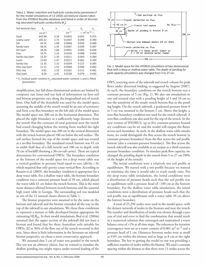
www.vadosezonejournal.org · Vol. 8, No. 1, February 2009 66
simplifi cation, but full three-dimensional analyses are limited by
computer run times and our lack of information on how soil
and biomat properties vary along the longitudinal axis of trench
lines. One half of the drainfi eld was used for the model space,
assuming the middle of the trench would be an axis of symmetry
and form a no-fl ux boundary on the left side of the model space.
Th e model space was 300 cm in the horizontal dimension. Th is
placed the right boundary at a suffi ciently large distance from
the trench that the contours of total potential near the trench
had ceased changing before the wetting front reached the right
boundary. Th e model space was 200 cm in the vertical dimension
with the trench bottom placed 100 cm below the soil surface. Th e
soil surface formed the top of the model space and was treated
as a no-fl ux boundary. Th e simulated trench bottom was 45 cm
in width (half that of a full trench) and 100 cm in depth, with
70 cm of backfi ll (forming a 30-cm-tall cavity). Th ese are typical
dimensions for conventional OWSs. Th e boundary condition
at the bottom of the model space for a deep water table was
a vertical gradient in pressure head equal to zero (dh/dz = 0),
which required that only gravity cause vertical fl ow. According to
Rassam et al. (2003), this boundary condition is appropriate for a
deep water table. For a shallow water table, the bottom boundary
condition was a constant pressure head of 39 cm, which placed
the water table 61 cm below the trench bottom. Th is is the mini-
mum distance allowed between trench bottoms and the seasonal
high water table in Georgia. Th e surrounding soil was modeled
as one of the 12 textural classes shown in Table 1.
Th e biomat properties were assumed to be the same on the
bottom and sidewall and the biomat extended all the way to the
top of the sidewall in our simulations. We chose these conditions
to represent a mature or fully developed biomat appropriate for
estimating HLRD. In their model simulations, Beal et al. (2004a)
assumed that the upper section of the sidewall did not have a
biomat and found that for three Australian soils suitable for
OWSs, 82 to 96% of the fl ow out of the trench occurred in this
area. Since there is little information in the literature on sidewall
biomat properties, we chose a more conservative approach.
We assumed that 5 cm of water was ponded in the trench.
Th is too was an arbitrary choice, but we wanted to simulate the
shallow ponding one might expect under normal loading of the
OWS, reserving most of the sidewall and trench volume for peak
fl ows under abnormal loading, as suggested by Siegrist (2007).
As such, the boundary condition on the trench bottom was a
constant pressure of 5 cm (Fig. 1). We also ran simulations in
one soil textural class with a ponding height of 1 and 10 cm to
test the sensitivity of the steady trench bottom fl ux to the pond-
ing height. On the trench sidewall, a graduated pressure from 0
to 5 cm was assumed in the bottom 5 cm. Above this height, a
zero-fl ux boundary condition was used for the trench sidewall. A
zero-fl ux condition was also used for the top of the trench. In the
new version of HYDRUS, up to fi ve constant-pressure bound-
ary conditions can be set and the model will output the fl uxes
across each boundary. As such, in the shallow water table simula-
tions, we could distinguish the fl ux across the trench bottom (a
constant-pressure boundary) from the fl ux across the soil profi le
bottom (also a constant-pressure boundary). Th e fl ux across the
trench sidewall was also available as an output as a third constant-
pressure boundary condition. To simulate peak fl ow capacity, we
changed the ponding depth in the trench from 5 to 27 cm (90%
of the height of the trench).
Th e initial conditions were a relatively wet soil profi le at
equilibrium. We started with a wet profi le because we wanted
to minimize the time it would take to reach steady state. For
the deep water table simulations, the initial conditions were
a distribution of pressure heads such that the soil profi le was
at equilibrium with a pressure head of −100 cm at the bottom
boundary. For the shallow water table simulations, the initial
conditions were a distribution of pressure heads such that the
soil profi le was at equilibrium with a water table 39 cm above
the bottom boundary.
A total of 25,296 nodes were used in the model space, with
the densest network of nodes in the biomats and near the trench.
Th e number and distribution of nodes was chosen through a pro-
cess of trial and error to fi nd the combination that would result
in a numerical solution that converged and maintained a water
balance error of <1% at all time steps. Th e tolerances for iteration
convergence were set at a water content of 0.001 m3 m−3 and a
pressure head of 1 cm. Distances between nodes were as small
as 0.05 cm within the biomat and as large as 8 cm at the right
boundary. Th e key to getting the model to run was providing a
suffi cient number of nodes within the biomat. We used a constant
spacing within the biomat so that there were 11 nodes across the
T 1. Water reten on and hydraulic conduc vity parameters† for the model simula ons of 12 USDA soil textural classes taken from the HYDRUS Rose a database and listed in order of decreas-ing saturated hydraulic conduc vity (Ks).
Soil textural class Ks n α θr θs
cm d−1 cm−1 — m3 m−3 —Sand 642.98 3.18 0.0353 0.053 0.375Loamy sand 105.12 1.75 0.0347 0.049 0.390Silt 43.74 1.68 0.0066 0.050 0.489Sandy loam 38.25 1.45 0.0267 0.039 0.387Silt loam 18.26 1.66 0.0051 0.065 0.439Clay 14.75 1.25 0.0150 0.098 0.459Sandy clay loam 13.19 1.33 0.0211 0.063 0.384Loam 12.04 1.47 0.0111 0.061 0.399Sandy clay 11.35 1.21 0.0334 0.117 0.385Silty clay loam 11.11 1.52 0.0084 0.090 0.482Silty clay 9.61 1.32 0.0162 0.111 0.481Clay loam 8.18 1.41 0.0158 0.079 0.442
† θr, residual water content; θs, saturated water content; α and n, fi ed parameters.
F . 1. Model space for the HYDRUS simula ons of two-dimensional fl ow with a deep or shallow water table. The depth of ponding for peak capacity simula ons was changed from 5 to 27 cm.
www.vadosezonejournal.org · Vol. 8, No. 1, February 2009 67
0.5-cm-thick biomat. Th e same fi nite element mesh was used for
all simulations. With a suffi ciently high density of nodes within
the biomat, it was not necessary to use the option of an air-entry
value of −2 cm with the K(h) function for clayey soils, unlike our
simulations in Radcliff e and West (2007).
We also ran a series of simulations where the model space
consisted of only the region below the trench. Th is was designed
to simulate purely vertical fl ow below the trench. Boundary and
initial conditions were the same as the deep water table simula-
tions described above. By comparing the simulations using the
region below the trench with the full simulations, the eff ect of
two-dimensional fl ow below the trench on the steady-state fl ux
through the trench bottom could be isolated.
To test the eff ect of soil heterogeneity, we used the stochastic
scaling factors feature in HYDRUS. Th is implements a scaling
procedure that assigns hydraulic parameter values to nodes in a
random manner such that the overall mean coincides with the
desired value but the distribution has a standard deviation set by
the user. We used the data from Schoeneberger and Amoozegar
(1990) to decide on what standard deviation to use for the soil
hydraulic conductivity. Th ese researchers reported on a study
where Ks was measured by horizon in soils of the Piedmont region
of North Carolina. We used the averaged data from two horizons:
a clay Bt and a clay loam B/C horizon. Pooling the values for
diff erent orientations and geomorphic positions, the mean Ks for
the clay horizon (based on a lognormal distribution) was 12.03
cm d−1 with a CV of 0.66. Th is mean Ks was quite close to the
clay textural class value from the HYDRUS database (14.75 cm
d−1 in Table 1). Th e mean Ks for the clay loam horizon was 0.333
cm d−1 with a CV of 3.17. Th is mean Ks was considerably lower
than the value for the clay loam textural class in the HYDRUS
database (8.18 cm d−1 in Table 1). Th e HYDRUS model assumes
a lognormal distribution of scaling factors. To convert the data
CV to a lognormal distribution standard deviation (σ), we used
the relationship given in Jury and Horton (2004):
( )= σ −2CV exp 1 [4]
Th is produced a scaling factor σ of 0.60 for the clay and
1.55 for the clay loam. Since the largest value that can be
used for σ is 1.00 in HYDRUS, we used that value for the
clay loam. We ran simulations for the clay and clay loam
textural classes using the soil parameter values in Table 1,
but specifi ed these values of σ for Ks. We ran fi ve “realiza-
tions” by recalculating the value for Ks at each node based
on the same σ each time before running the simulation.
We compared the trench bottom fl uxes in the simulations
including soil heterogeneity to simulations that did not
include soil heterogeneity. Scaling factors can be used for
water content and pressure head as well as for hydraulic
conductivity in HYDRUS. We did not use scaling factors
for these other two hydraulic parameters because these
parameters are much less variable than hydraulic conduc-
tivity (Jury and Horton, 2004).
Bouma Equa ons
Equation [1] (Bouma, 1975) was used to estimate
steady fl ux through the bottom of the trench for each soil
textural class for comparison with the steady-state fl ux
found by HYDRUS. In this equation, we used Kbs = 0.23 cm d−1,
Zb = 0.5 cm, h0 = 5 cm, and the K(h) function was expressed using
Eq. [3] with the parameters Ks, m = 1 − 1/n, α, θr, and θs taken
from Table 1 for the appropriate soil. When this was done, hs
appeared on both sides of the equation as an unknown. We then
used the Minerr function in Mathcad (Parametric Technology
Corp., Needham, MA) to solve for hs. Once hs was known, the
Bouma estimate of fl ux through the trench bottom was equal
to K(hs). We found that it was necessary to modify Eq. [1] to
account for unsaturated fl ow in the biomat and these modifi ca-
tions are described below.
Results and Discussion
HYDRUS Simula ons of Steady Trench Bo om Flux
HYDRUS automatically adjusts the time steps (within user-
specifi ed limits) to maintain an accurate water balance within the
model space so that run times for simulations vary, depending on
the diffi culty of the numerical problem. Run times to reach 30
d for the HYDRUS deep water table simulations with 5 cm of
ponded water in the trench varied substantially with soil textural
class. Using a Pentium 4 computer, the shortest run time was for
the silt class (665 s) and the longest run time was for the sandy
clay class (7879 s). Run times for the shallow water table simula-
tions were much shorter and in a narrow range from 230 to 321
s for all the soils except the sandy clay, which required the longest
time of any of the shallow ponding simulations, 12,307 s. Th e
longest run times were for the estimation of peak capacity when
water in the trench was ponded to a depth of 27 cm. Many of
these simulations ran >48 h and we stopped the runs before they
reached 30 d as long as the fl uxes out of the trench bottom and
sidewall had reached steady rates.
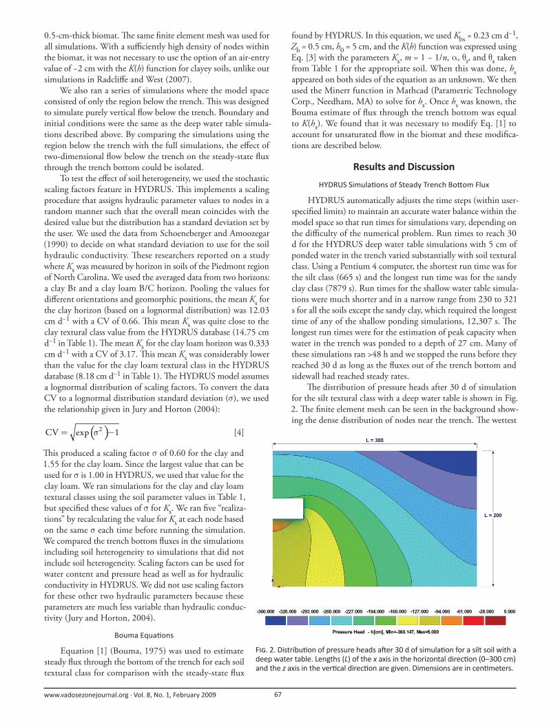
Th e distribution of pressure heads after 30 d of simulation
for the silt textural class with a deep water table is shown in Fig.
2. Th e fi nite element mesh can be seen in the background show-
ing the dense distribution of nodes near the trench. Th e wettest
F . 2. Distribu on of pressure heads a er 30 d of simula on for a silt soil with a deep water table. Lengths (L) of the x axis in the horizontal direc on (0–300 cm) and the z axis in the ver cal direc on are given. Dimensions are in cen meters.
www.vadosezonejournal.org · Vol. 8, No. 1, February 2009 68
region (highest pressure head) was imme-
diately below the trench and confi ned to a
relatively small hemispherical contour (Fig.
2). Contours of drier soil extended to the
right and above the trench, indicating that
capillarity had drawn water laterally and
even up into dry soil regions as the water
infi ltrated through the sidewall. Within the
wettest contour below the trench, pressure
heads varied between about −85 and −90
cm so that the entire profile remained
unsaturated, even after 30 d of infiltra-
tion. Th e silt textural class had the highest
steady-state infi ltration rate through the
trench bottom in the deep water table sim-
ulations (Table 2). Fluxes across the trench
boundaries were high at the beginning of
the simulation but declined to a steady rate
after about 3 d for both the trench bottom
and sidewall.
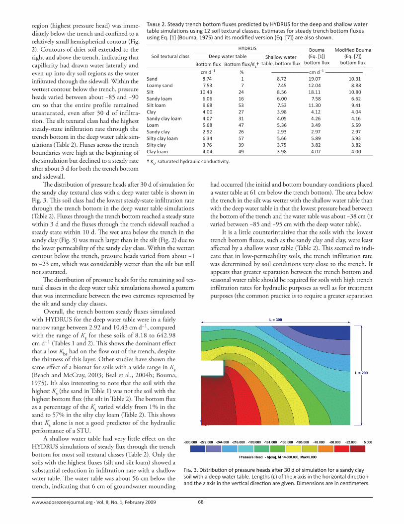
Th e distribution of pressure heads after 30 d of simulation for
the sandy clay textural class with a deep water table is shown in
Fig. 3. Th is soil class had the lowest steady-state infi ltration rate
through the trench bottom in the deep water table simulations
(Table 2). Fluxes through the trench bottom reached a steady state
within 3 d and the fl uxes through the trench sidewall reached a
steady state within 10 d. Th e wet area below the trench in the
sandy clay (Fig. 3) was much larger than in the silt (Fig. 2) due to
the lower permeability of the sandy clay class. Within the wettest
contour below the trench, pressure heads varied from about −1
to −23 cm, which was considerably wetter than the silt but still
not saturated.
Th e distribution of pressure heads for the remaining soil tex-
tural classes in the deep water table simulations showed a pattern
that was intermediate between the two extremes represented by
the silt and sandy clay classes.
Overall, the trench bottom steady fl uxes simulated
with HYDRUS for the deep water table were in a fairly
narrow range between 2.92 and 10.43 cm d−1, compared
with the range of Ks for these soils of 8.18 to 642.98
cm d−1 (Tables 1 and 2). Th is shows the dominant eff ect
that a low Kbs had on the fl ow out of the trench, despite
the thinness of this layer. Other studies have shown the
same eff ect of a biomat for soils with a wide range in Ks
(Beach and McCray, 2003; Beal et al., 2004b; Bouma,
1975). It’s also interesting to note that the soil with the
highest Ks (the sand in Table 1) was not the soil with the
highest bottom fl ux (the silt in Table 2). Th e bottom fl ux
as a percentage of the Ks varied widely from 1% in the
sand to 57% in the silty clay loam (Table 2). Th is shows
that Ks alone is not a good predictor of the hydraulic
performance of a STU.
A shallow water table had very little eff ect on the
HYDRUS simulations of steady fl ux through the trench
bottom for most soil textural classes (Table 2). Only the
soils with the highest fl uxes (silt and silt loam) showed a
substantial reduction in infi ltration rate with a shallow
water table. Th e water table was about 56 cm below the
trench, indicating that 6 cm of groundwater mounding
had occurred (the initial and bottom boundary conditions placed
a water table at 61 cm below the trench bottom). Th e area below
the trench in the silt was wetter with the shallow water table than
with the deep water table in that the lowest pressure head between
the bottom of the trench and the water table was about −38 cm (it
varied between −85 and −95 cm with the deep water table).
It is a little counterintuitive that the soils with the lowest
trench bottom fl uxes, such as the sandy clay and clay, were least
aff ected by a shallow water table (Table 2). Th is seemed to indi-
cate that in low-permeability soils, the trench infi ltration rate
was determined by soil conditions very close to the trench. It
appears that greater separation between the trench bottom and
seasonal water table should be required for soils with high trench
infi ltration rates for hydraulic purposes as well as for treatment
purposes (the common practice is to require a greater separation
F . 3. Distribu on of pressure heads a er 30 d of simula on for a sandy clay soil with a deep water table. Lengths (L) of the x axis in the horizontal direc on and the z axis in the ver cal direc on are given. Dimensions are in cen meters.
T 2. Steady trench bo om fl uxes predicted by HYDRUS for the deep and shallow water table simula ons using 12 soil textural classes. Es mates for steady trench bo om fl uxes using Eq. [1] (Bouma, 1975) and its modifi ed version (Eq. [7]) are also shown.
Soil textural class
HYDRUS Bouma (Eq. [1])
bo om fl ux
Modifi ed Bouma(Eq. [7])
bo om fl uxDeep water table Shallow water
table, bo om fl uxBo om fl ux Bo om fl ux/Ks†
cm d−1 % —————————— cm d−1 ——————————Sand 8.74 1 8.72 19.07 10.31Loamy sand 7.53 7 7.45 12.04 8.88Silt 10.43 24 8.56 18.11 10.80Sandy loam 6.06 16 6.00 7.58 6.62Silt loam 9.68 53 7.53 11.30 9.41Clay 4.00 27 3.98 4.12 4.04Sandy clay loam 4.07 31 4.05 4.26 4.16Loam 5.68 47 5.36 3.49 5.59Sandy clay 2.92 26 2.93 2.97 2.97Silty clay loam 6.34 57 5.66 5.89 5.93Silty clay 3.76 39 3.75 3.82 3.82Clay loam 4.04 49 3.98 4.07 4.00
† Ks, saturated hydraulic conduc vity.

www.vadosezonejournal.org · Vol. 8, No. 1, February 2009 69
distance for sandy soils to reduce pollutant levels before reaching
the groundwater).
Bouma Equa on Es mate of Steady Trench Bo om Flux
Th e estimated steady bottom fl uxes for the various soils using
the Bouma (1975) Eq. [1] are shown in Table 2 and plotted
against the HYDRUS simulated fl uxes for the deep water table
simulations in Fig. 4. Bouma’s equation accurately estimated trench
bottom fl uxes in the soil textural classes with low fl uxes but consid-
erably overestimated the fl ux in the fi ve textural classes with high
fl uxes: sand, silt, loamy sand, silt loam, and sandy loam.
Th ere are three simplifying assumptions in the Bouma (1975)
equation that are potential sources of error in estimating steady
bottom fl ux. Th ese assumptions are: a unit gradient (dh/dz = 0)
in the soil immediately below the biomat, saturated conditions in
the biomat, and one-dimensional vertical fl ow within the biomat
and the soil beneath the biomat. Since the HYDRUS simulations
do not make these assumptions, we could investigate their validity
by examining the simulation results. Pressure heads within the
biomat and immediately below the biomat midway between the
trench centerline and the trench sidewall in the HYDRUS simu-
lation of the sand textural class with a deep water table after 30
d are shown in Fig. 5. Below the biomat, the pressure heads are
constant at a value of about −44 cm. Th e constant values satisfy
the assumption that dh/dz = 0. Because of the large number of
nodes within the biomat cross-section, we were able to see clearly
the distribution of pressure heads within the biomat (the top 0.5
cm of the transect). Th ey were negative for most of the biomat
and reached the minimum pressure of −44 cm at the bottom of
the biomat. Th is indicated that the assumption of a saturated
biomat hydraulic conductivity (Kbs) in Eq. [1] was not valid and
could lead to an overestimation of the bottom fl ux. We modifi ed
Eq. [1] to account for unsaturated fl ow within the biomat by
substituting an eff ective biomat hydraulic conductivity (Kb eff )
appropriate for hydraulic resistances in series (Jury and Horton,
2004) in Eq. [1] for Kbs:
( )=
=⎡ ⎤⎣ ⎦∑
beff
b1
1
1k
ii
KkK h
[5]
where Kb(hi) is the unsaturated hydraulic conductivity for the
biomat in layer i and k is the number of subdivisions (of uniform
thickness) in the biomat. Th is function was based on the van
Genuchten (1980) equation we used for soil K(h) (Eq. [3]) with
Kbs for the saturated hydraulic conductivity of the biomat and
the retention parameters (θr, θs, α, and n) for the loam textural
class. Based on Fig. 5 (and similar plots for the other soil textural
classes), we assumed that the distribution of h within the biomat
could be described by a parabolic equation that has a value of h0 at the
top of the biomat and a value of hs at the bottom of the biomat:
( )⎡ ⎤−⎢ ⎥= − +⎢ ⎥⎣ ⎦
2s 0 b
02b
1i
h h Zh i h
kZ [6]
Th is distribution is shown in Fig. 5 for comparison with the dis-
tribution obtained in the HYDRUS simulations. Substituting Eq.
[5] and [6] into Eq. [1], we obtained
( )
( )=
− +⎛ ⎞⎧ ⎫⎪ ⎪⎡ ⎤ ⎟−⎜ ⎪ ⎪⎟⎜ − +⎢ ⎥ ⎟⎨ ⎬⎜ ⎟⎜ ⎪ ⎪⎢ ⎥ ⎟⎟⎜ ⎣ ⎦⎪ ⎪⎝ ⎠⎩ ⎭
=
∑
0 s b
2bs 0 b
b 021 b
s
1
1 1k
i
h h Z
Zh h ZkK i h
kZ
K h
[7]
We subdivided the biomat into fi ve even layers (k = 5) for all
our calculations.
Th e estimated steady fl uxes for the various soils using the
modifi ed Bouma Eq. [7] for bottom fl ux are shown in Table 2
and plotted against the HYDRUS simulated fl uxes for the deep
water table simulations in Fig. 6. Th e modifi ed equation improved
the agreement with the HYDRUS estimates, as indicated by the
improved r2, the regression line intercept near zero, and the slope
F . 4. Es mate of steady trench bo om fl ux obtained from Eq. [1] (Bouma, 1975) vs. HYDRUS-simulated trench bo om fl ux for 12 soil textural classes. The dashed line is the 1:1 line. The solid line is the least squares regression line for which the equa on and r2 are shown.
F . 5. Ver cal transect of pressure heads below the trench at a point midway between the trench centerline and the sidewall in the HYDRUS simula on of the sand soil with a deep water table a er 30 d (solid blue line with solid circles). Also shown is the assumed distribu on of pres-sure heads in the modifi ed Bouma equa on (Eq. [7]) (solid red line).

www.vadosezonejournal.org · Vol. 8, No. 1, February 2009 70
near one as shown in Fig. 6. Th e modifi cation reduced fl uxes in
the soil textural classes with high fl uxes but had little eff ect on
the classes with low fl uxes. Th is was because, in the soil classes
with low fl uxes, there was less of a diff erence between Kbs and Ks.
As a result, hs was closer to zero and there was less desaturation
in the biomat and less of a reduction in the eff ective hydraulic
conductivity of the biomat.
We tested for the third source of error in the Bouma (1975)
equation (i.e., assuming no lateral fl ow below the trench bottom)
by comparing the simulations described so far with simulations
using the model space confi ned to the area below the trench, which
restricted fl ow to the vertical dimension. Th e ratio of steady bottom
fl uxes (two-dimensional/one-dimensional) ranged from 1.0 in the
sand textural class to 1.17 in the silt loam. We would expect lateral
fl ow and the eff ect of a relatively dry region of soil surrounding the
trench corner to be least in a sand where capillarity is at a mini-
mum. Th us, lateral fl ow was only a very minor source of error in
using the original or the modifi ed Bouma equations. For narrower
trenches, however, we would expect a greater lateral fl ow eff ect.
Th e modifi ed Bouma equation provided a simple method for
estimating the steady fl ux through the trench bottom and also
provided insight into the HYDRUS simulations. Th e reason why
the silt textural class had the highest fl ux (despite the fact that
it did not have the highest Ks) was apparent when the modifi ed
Bouma equation for fl ux through the biomat was plotted with the
unsaturated hydraulic conductivity curves of the diff erent soils as
a function of pressure head (Fig. 7). Th e unsaturated hydraulic
conductivity curves are based on the parameters in Table 1. Th e
modifi ed Bouma estimates of fl ux are the values of K(h) where the
biomat fl ux curve intersects the K(h) curves. It is clear that the silt
textural class had the highest bottom fl ux because it had a rela-
tively high Ks and a K(h) curve that dropped off slowly, typical of
a medium-textured soil. Th is also applied to the silt loam textural
class. Th e sand and loamy sand soils had high estimated fl uxes
in spite of relatively steep K(h) curves due to their high Ks. Th e
sandy clay had the lowest estimated fl ux due to a low Ks and a
steep K(h) curve. Th e other soil textural classes had intermediate
K(h) curves and estimated fl uxes.
With Fig. 7 in mind, it’s easier to think about what eff ect a
higher or lower fl ux through the biomat might have on steady
trench bottom fl uxes and the order of the soil textural classes.
If the biomat is more conductive or thinner, or more water is
ponded in the trench, the biomat fl ux curve will move higher
in Fig. 7. Th is will push the point of intersection with the K(h)
curves closer to the y axis and the order of the soil textural classes
in terms of trench bottom fl uxes will more closely resemble the
order of Ks (it will be a better predictor of trench hydraulic per-
formance). Conversely, anything that reduces the fl ux through the
biomat will lower the biomat fl ux curve and Ks will be a poorer
predictor of hydraulic performance
Th e modifi ed Bouma equation (Eq. [7]) underpredicted
steady trench bottom fl ux in the silt and silt loam textural classes
for a shallow water table, but accurately predicted the fl ux for all
the other textural classes (Table 2). Th is was due to the assump-
tion (in the original as well as the modifi ed equations) that dh/
dz = 0 just below the trench. For these two soils with the highest
trench bottom fl uxes, a shallow water table reduced the pressure
head gradient slightly (dh/dz < 0) just below the biomat and
consequently Eq. [7] overestimated the bottom fl ux.
Biomat and Ponding Height Sensi vity Analysis
Increasing the Kbs 10-fold to 2.30 cm d−1 in the loam soil
textural class HYDRUS simulation with a deep water table
increased the steady trench bottom fl ux from 4.68 to 14.30 cm
F . 6. Bouma Eq. [7] es mate of steady trench bo om fl ux vs. HYDRUS-simulated fl ux for 12 soil textural classes. The dashed line is the 1:1 line. The solid line is the least squares regression line for which the equa on and r2 are shown.
F . 7. Unsaturated hydraulic conduc vity func ons for the 12 soil textural classes vs. pressure head. Also shown is the modifi ed Bouma equa on for fl ux through a biomat. The intersec on of the hydraulic conduc vity curve for a par cular soil and the Bouma curve gives the steady-state fl ux.

www.vadosezonejournal.org · Vol. 8, No. 1, February 2009 71
d−1. Assuming that the biomat water retention parameters
were the same as the soil simulated (but keeping Kbs at 0.23
cm d−1) resulted in a slightly wider range of steady trench
bottom fl uxes for all of the soil textural class simulations
with a deep water table (2.64–16.54 cm d−1) compared
with the simulations with a uniform loam-textured biomat
(2.92–10.43 cm d−1, Table 2). Th ese results showed that
Kbs was more important than the biomat water retention
parameters. Changing the ponding height in the trench
to 1 and 10 cm produced steady trench bottom fl uxes of
4.70 and 7.01 cm d−1 in the loam soil with a deep water
table, which were relatively close to the fl ux with 5 cm
of ponded water (5.68 cm d−1, Table 2), indicating that
ponding height was not a sensitive input variable.
Soil Heterogeneity
Th e eff ect of including soil heterogeneity on the dis-
tribution of pressure heads after 2 d is shown in Fig. 8
for the clay textural class with a deep water table after
2 d. Th e contour lines of pressure head are much more
variable than in the simulations where heterogeneity in
Ks was not included (Fig. 2–3). Th e mean trench bottom
fl ux for fi ve simulations with separate realizations of the
random values of Ks assigned to each node was 5.01 cm
d−1, compared with the fl ux for the simulations with uniform Ks
of 4.00 cm d−1 (see clay textural class in Table 2). Th e standard
deviation for the trench bottom fl ux in the fi ve realizations was
relatively small, 0.05 cm d−1. For the clay loam textural class,
the mean trench bottom fl ux for fi ve realizations was 6.17 cm
d−1, compared with 4.04 cm d−1 for simulations that did not
include heterogeneity (see clay loam textural class in Table 2), also
with a standard deviation of 0.05 cm d−1. Th us, including soil
heterogeneity increased the steady trench bottom fl ux by 25 to
53%. Basing HLRD on estimates of fl uxes in homogeneous soils
is therefore likely to underestimate the hydraulic performance
of soils with a high degree of heterogeneity, such as structured
clays. In this sense, assuming homogeneous soils results in a con-
servative estimate of the hydraulic performance but it probably
overestimates the capacity of the soil to treat wastewater (the
organic loading component of the LTAR).
Peak Flow Capacity
Our HYDRUS simulations of a trench nearly full of effl u-
ent (ponded to 27 cm) for the sand class showed that the total
fl ow out of the trench (including bottom and sidewalls) reached
a steady state of 1182 cm3 d−1 cm−1 of trench length in the
longitudinal (z axis) direction. Th is was 2.71 times the total fl ow
out of the trench for the same soil class with 5 cm of ponded
effl uent. Th e largest ratio for peak fl ow occurred in the sandy
clay textural class, where peak fl ow was 4.78 times the fl ow out
of the trench with 5 cm of water ponded. Th e lowest ratio (1.81)
occurred in the silt loam textural class. Th ese results indicate that
peak capacity is two to fi ve times that of normal operating condi-
tions (shallow ponding). Our simulations assumed that sidewall
biomat properties are identical to bottom biomat properties. Th at
is probably not the case in that biomats on the upper sidewall are
probably more permeable, thinner, or both (Keys et al., 1998).
Under these conditions, peak capacity would be greater than what
we estimated.
Design Hydraulic Loading Rate
As a safety factor, we have taken 50% of the HYDRUS-
simulated trench bottom fl ux with a shallow water table (Table
2) and used that as a proposed HLRD in Table 3. Th e soil textural
classes are shown in order based on the HLRD in centimeters
per day as well as gallons per square foot per day (gal ft−2 d−1),
which are the common units used in regulations (state and local)
for HLRD. We have grouped the soils into four classes based on
HLRD (Table 3). In Class I are the four soils with HLRD values
near 4 cm d−1. In Class II are three soils with HLRD values in a
narrow range near 3 cm d−1. In Class III are four soils with HLRD
values in a narrow range near 2 cm d−1. Class IV consists of only
one soil textural class, but we believe that there are other soil
classes that would fall in this category in the southern Piedmont
region of the United States. An example is the clay loam horizon
F . 8. Distribu on of pressure heads a er 2 d of simula on for a clay soil with a deep water table and soil heterogeneity included. Lengths (L) of the x axis in the horizontal direc on and the z axis in the ver cal direc on are given. Dimensions are in cen meters.
T 3. Design hydraulic loading rates (HLRD) for 12 soil textural classes based on the trench bo om fl ux es mated in the HYDRUS simula ons for a shallow water table and the modifi ed Bouma Eq. [7]. The values were calculated as 50% of the fl uxes shown in Table 2. Based on the HLRD, soil textural classes were divided into Class I, II, III, or IV.
Soil textural classHLRD based on HYDRUS
simula ons, shallow water table
HLRD based on modifi ed Bouma
Eq. [7]Class
cm d−1 (gal −2 d−1) cm d−1 (gal −2 d−1)Sand 4.36 (1.07) 5.16 (1.26) ISilt 4.28 (1.05) 5.40 (1.32) ISilt loam 3.77 (0.92) 4.71 (1.15) ILoamy sand 3.73 (0.91) 4.44 (1.09) ISandy loam 3.00 (0.74) 3.31 (0.81) IISilty clay loam 2.83 (0.69) 2.97 (0.73) IILoam 2.68 (0.66) 2.79 (0.68) IISandy clay loam 2.03 (0.50) 2.08 (0.51) IIIClay loam 1.99 (0.49) 2.00 (0.49) IIIClay 1.99 (0.49) 2.02 (0.49) IIISilty clay 1.87 (0.46) 1.91 (0.47) IIISandy clay 1.46 (0.36) 1.48 (0.36) IV

www.vadosezonejournal.org · Vol. 8, No. 1, February 2009 72
in the study by Schoeneberger and Amoozegar (1990) with a Ks
of 0.333 cm d−1 as we mentioned above. Th e Rosetta database
from which we drew our soil parameters has relatively few records
for soils from the clayey region of the soil textural triangle (clay,
silty clay, and sandy clay) (Schaap et al., 2001), and the fl ux
through these soils may be overestimated in our analysis.
We also used the modifi ed Bouma Eq. [7] to determine the
HLRD by taking 50% of the estimated trench bottom fl uxes
shown in Table 2. Th e resulting values are shown in Table 3. Th e
order of the soils in terms of HLRD was exactly the same as that
based on the HYDRUS simulations except that the sand and silt
textural classes reversed order, as did the clay loam and clay tex-
tural classes. Th e only substantial diff erence in estimated HLRD
occurred with the silt and silt loam soils, where a shallow water
table reduced fl ux (as we discussed above). Th e soil classes (I–IV)
were the same whether we used the HYDRUS simulations or
the modifi ed Bouma Eq. [7]. In our opinion, taking 50% of the
trench bottom fl ux estimated by the modifi ed Bouma Eq. [7] serves
quite well as a basis for estimating HLRD and grouping soils.
Siegrist (2007) proposed that HLRD should vary with the
type of OWS: a conventional system (Type I), a system with an
aerobic treatment unit or constructed wetland (Type II), and a
system with a packed bed fi lter or membrane bioreactor (Type
III), with the lowest rates for Type I systems. Since we simulated a
conventional OWS, we compared our values to the HLRD values
for Type I systems. Siegrist (2007) grouped soils into three classes
in terms of their HLRD (Table 4). Th e HLRD values ranged from
4 cm d−1 (1.0 gal ft−2 d−1) for Class I to 1.0 cm d−1 (0.25 gal ft−2
d−1) for Class III. Only seven of the 12 USDA textural classes
were included in that system.
Our values of HLRD in Table 3 ranged from 1.46 to 4.36 cm
d−1 (0.36–1.07 gal ft−2 d−1), which were quite close to the range
suggested by Siegrist (2007) (Table 4). Our system diff ers in that
it promotes the silt loam class to the highest category for HLRD
and promotes the silty clay loam and clay loam into the second
category. Th ese changes are due to the importance of unsaturated
hydraulic conductivity in determining the hydraulic performance
of these textural classes. Our analysis also provides information
on soil textural classes that were not included in Siegrist (2007).
Lindbo et al. (2007) described a decision-tree method for
determining the LTAR for OWSs in North Carolina. Th e method
consists of 10 steps, with the last step being an adjustment for
effl uent quality and dispersal method so that the fi rst nine steps
are a determination of the HLRD. Th ey used four groups for soils
and assigned a range and midpoint for HLRD. Th e midpoint
values for HLRD ranged from 4 cm d−1 (1.0 gal ft−2 d−1) for Class
I to 1.0 cm d−1 (0.25 gal ft−2 d−1) for Class IV. Th ese values are
also quite close to the range we propose and we have adopted
midpoint values for our four classes very similar to those in the
North Carolina system (Table 4). Our results suggest, however,
that the silt and silt loam soils should be moved from Class III
to Class I, the silty clay loam soil should be moved from Class
III to Class II, and the silty clay and clay should be moved from
Class IV to Class III. Th is would more accurately refl ect the high
infi ltration capacities of these soils.
ConclusionsWe found that the HYDRUS model or a modifi ed form of
the Bouma (1975) equation could be used to develop HLRD
values for OWSs based on soil hydraulic properties. Th e HYDRUS
simulations with 12 soil textural classes showed that steady trench
bottom fl uxes were in a fairly narrow range of 2.92 to 10.43 cm
d−1 with a deep water table, despite the wide range in Ks for these
soils of 8.18 to 642.98 cm d−1. Th is indicated the importance of a
biomat in restricting fl ow in OWSs. Saturated hydraulic conduc-
tivity was not a good predictor of trench bottom fl ux in that fl ux
as a percentage of Ks varied from 1 to 57%. A shallow water table
did not reduce the steady trench bottom fl ux except for the two
soil textural classes with the highest fl uxes: the silt and silt loam
textural classes. Th e Bouma (1975) equation, modifi ed to account
for unsaturated conditions in the biomat, accurately predicted
trench bottom fl uxes in all cases except the shallow water table
simulations with the silt and silt loam textural classes. Including
soil heterogeneity increased trench bottom fl uxes by 25 to 53%,
depending on the assumed degree of heterogeneity. Th erefore,
analyses such as ours that are based on assumptions of homoge-
neous soils are a conservative estimate of hydraulic performance.
Peak capacity with a nearly full trench was estimated to be two
to fi ve times the total infi ltration rate (trench bottom fl ow plus
sidewall fl ow) with 5 cm of water ponded in the trench. Th is is a
conservative estimate of peak capacity in that biomat properties
near the top of the sidewall are unlikely to be as fully developed
as those at the bottom of the trench.
To convert the steady trench bottom fl ux to a HLRD, we
took 50% of the fl ux simulated with HYDRUS or estimated
with the modifi ed Bouma (1975) equation. We then grouped
the 12 soil textural classes into four classes based on HLRD. Our
HLRD values ranged from 1.46 to 4.36 cm d−1 (0.36–1.07 gal
ft−2 d−1), which was very close to the systems proposed by Siegrist
(2007) and Lindbo et al. (2007). Our results diff er from these
T 4. Soil classes and design hydraulic loading rates (HLRD) for systems that are in use by states or have been proposed compared with our analysis.
System Class I Class II Class III Class IVSiegrist (2007) HLRD, cm d−1 (gal 2 d−1) 4 (1) 2 (0.5) 0.5 (0.12) Soil classes sand, loamy sand sandy loam, loam, silt loam silty clay loam, clay loamLindbo et al. (2007) HLRD, cm d−1 (gal 2 d−1) 4 (1) 3 (0.7) 1.8 (0.45) 1 (0.25) Soil classes sand, loamy sand sandy loam, loam silt loam, clay loam, sandy clay
loam, silty clay loam, siltsandy clay, silty clay, clay
Our analysis HLRD, cm d−1 (gal 2 d−1) 4 (1) 3 (0.75) 2 (0.50) 1 (0.25) Soil classes Sand, silt, silt loam,
loamy sandsandy loam, silty clay loam,
loamsandy clay loam, clay loam,
clay, silty claysandy clay
www.vadosezonejournal.org · Vol. 8, No. 1, February 2009 73
other systems primarily in that we show that medium-textured
soils with intermediate Ks should be in the higher categories for
HLRD due to their unsaturated hydraulic properties.
In this study, we are recommending a system for determining
HLRD rather than a particular set of values. Th ere are a number
of choices that can be made so that the method can be tailored
to the needs of diff erent jurisdictions. Th e system can be based
on HYDRUS simulations or the modifi ed Bouma (1975) equa-
tion. In either case, one can decide on what level of ponding
to assume in the trench (we chose 5 cm) for normal operating
conditions. One can also choose the properties of the biomat
to use (thickness, saturated hydraulic conductivity, and water
retention parameters). Th e eff ect of diff erent OWS pretreatment
systems and architectures could be incorporated by assuming
diff erent biomat properties for these systems. In converting the
estimated trench bottom fl ux to a HLRD, one can choose the
percentage of the fl ux to use as a safety factor (we used 50%),
how many groups to use (we used four), and where to make the
cuts between groups. Th e important feature of the process we
propose is that the method for determining the HLRD is based
on quantifi able soil hydraulic properties and the assumptions
are evident (and can be changed as more information becomes
available, using an adaptive management approach). To facilitate
the use of the modifi ed Bouma (1975) equation, we have devel-
oped a spreadsheet that uses an iterative process to solve Eq. [7].
Th is spreadsheet, along with a guidance document, is posted on
our website at mulch.cropsoil.uga.edu/soilphysics/research.html
(verifi ed 21 Nov. 2008).
One of the fi ndings of this study and that of Heatwole and
McCray (2007) is the importance of the unsaturated hydraulic
properties of soils and biomats. To use the method we propose,
an estimate of the retention properties of a soil (θr, θs, α, and n in
our case) are required as well as the saturated hydraulic conduc-
tivity. Th ese values can be obtained from soil databases such as
Rosetta using just textural class, or a more accurate estimate can
be obtained using additional information about the soil such as
bulk density and the fi eld capacity and permanent wilting point
water contents. Th e literature on pedotransfer functions provides
a rich source of information on the unsaturated hydraulic proper-
ties of soils (Wösten et al., 2001) as well. Our work also shows
the need for more information on biomat hydraulic properties
(thickness, saturated hydraulic conductivity, retention properties,
uniformity, and rate of development).
Like all model studies, our fi ndings are based on a number
of assumptions that may not hold true under various fi eld condi-
tions. Our HYDRUS simulation model, with the use of soil data
from Rosetta, needs to be verifi ed against fi eld data. Also, we
could not separate out the eff ect of soil structure or clay mineral-
ogy (which some state and local regulations consider) in that the
textural class hydraulic parameters in the Rosetta database are
an average of all the soils within that textural class, which may
include varying degrees of structure and diff erent clay mineralo-
gies. Th e methods we present here (the model and the modifi ed
form of the Bouma equation), however, provide an approach for
developing HLRD values for OWSs based on soil hydraulic prop-
erties as an alternative to the conventional empirical approach
used by most states and local jurisdictions.
ReferencesAmoozegar, A., K. Martin, C. Niewoehner, and D. Lindbo. 2007. Wastewater
infi ltration and water movement around trenches of septic systems. In K.
Mancl (ed.) Individual and Small Community Sewage Syst. Conf. Proc.,
11th, Warwick, RI. 20–24 Oct. 2007. ASABE Publ. 701P1107. Am. Soc.
Agric. Biol. Eng., St. Joseph, MI.
Beach, D.N.H., and J.E. McCray. 2003. Numerical modeling of unsaturated
fl ow in wastewater soil absorption systems. Ground Water Monit. Reme-
diat. 23:64–72.
Beal, C.D., T. Gardner, N.W. Menzies, D. Rassam, and A. Vieritz. 2004a.
Prediction of steady-state fl ux through variably saturated zones within a
septic absorption trench. Available at http://regional.org.au/au/asssi/super-
soil2004/s15/oral/1663_bealc.htm (verifi ed 17 Nov. 2008). In B. Singh
(ed.) SuperSoil 2004, Sydney, Australia. 5–9 Dec. 2004. Regional Inst.,
Gosford, NSW, Australia.
Beal, C.D., E.A. Gardner, A. Vieritz, and N.W. Menzies. 2004b. Th e role of
the biomat in the sustainable performance of soil absorption systems in
Australia: A review. p. 241–248. In K. Mancl (ed.) Individual and small
Community Sewage Systems, 10th, Sacremento, CA. 21–24 Mar. 2004.
Am. Soc. Agric. Biol. Eng., St Joseph, MI.
Beal, C.D., D.W. Rassam, E.A. Gardner, G. Kirchof, and N.W. Menzies. 2008.
Infl uence of hydraulic loading and effl uent fl ux on surface surcharging of
soil absorption systems. J. Hydrol. Eng. 13:681–692.
Bouma, J. 1975. Unsaturated fl ow during soil treatment of septic tank effl uent.
J. Environ. Eng. Div. Am. Soc. Civ. Eng. 101:967–983.
Bumgarner, J., and J.E. McCray. 2007. Estimating biozone hydraulic conductiv-
ity in wastewater soil-infi ltration systems using inverse numerical model-
ing. Water Res. 41:2349–2360.
Finch, S.D., D.E. Radcliff e, and L.T. West. 2008. Modeling trench sidewall and
bottom fl ow in on-site wastewater systems. J. Hydrol. Eng. 13:693–701.
Finch, S.D., L.T. West, D.E. Radcliff e, and E.V. Hufstetler. 2007. Th ickness and
hydraulic properties of drainfi eld trench biomats formed in Georgia soils.
In K. Mancl (ed.) Individual and Small Community Sewage Syst. Conf.
Proc., 11th, Warwick, RI. 20–24 Oct. 2007. ASABE Publ. 701P1107. Am.
Soc. Agric. Biol. Eng., St. Joseph, MI.
Heatwole, K.K., and J.E. McCray. 2007. Modeling potential vadose-zone trans-
port of nitrogen from onsite wastewater systems at the development scale
J. Contam. Hydrol. 91:184–201.
Jenssen, P.D., and R.L. Siegrist. 1991. Integrated loading rate determination for
wastewater infi ltration system sizing. p. 182–191. In On-site Wastewater
Treatment: Proc. Natl. Symp. on Individual and Small Community Sew-
age Systems, 6th, Chicago, IL. 16–17 Dec. 1991. Am. Soc. Agric. Eng.,
St. Joseph, MI.
Jury, W.A., and R. Horton. 2004. Soil physics. 6th ed. John Wiley & Sons,
Hoboken, NJ.
Keys, J.R., E.J. Tyler, and J.C. Converse. 1998. Predicting life for wastewater
absorption systems. p. 167–176. In Proc. Natl. Symp. on Individual And
Small Community Sewage Systems, 8th, Orlando, FL. 8–10 Mar. 1998.
ASAE Publ. 10–91:192–200. Am. Soc. Agric. Eng., St. Joseph, MI.
Lindbo, D.L., J. Lynn, K. Neal, G. Young, and A. Amoozegar. 2007. Applying
soil morphology to long term acceptance rate determination. In K. Mancl
(ed.) Individual and Small Community Sewage Syst. Conf. Proc., 11th,
Warwick, RI. 20–24 Oct. 2007. ASABE Publ. 701P1107. Am. Soc. Agric.
Biol. Eng., St. Joseph, MI.
Radcliff e, D.E., and L.T. West. 2007. Modeling long term acceptance rates for
OWMSs. In K. Mancl (ed.) Individual and Small Community Sewage
Syst. Conf. Proc., 11th, Warwick, RI. 20–24 Oct. 2007. ASABE Publ.
701P1107. Am. Soc. Agric. Biol. Eng., St. Joseph, MI.
Radcliff e, D.E., L.T. West, and J. Singer. 2005. Gravel eff ect on wastewater infi l-
tration from septic system trenches. Soil Sci. Soc. Am. J. 69:1217–1224.
Rassam, D., J. Šimůnek, and M.Th . van Genuchten. 2003. Modeling variably
saturated fl ow with HYDRUS-2D. ND Consulting, Brisbane, Australia.
Richards, L.A. 1931. Capillary conduction of liquids in porous mediums. Phys-
ics 1:318–333.
Schaap, M.G., F.J. Leij, and M.Th . van Genuchten. 2001. Rosetta: A computer
program for estimating soil hydraulic parameters with hierarchical pedo-
transfer functions. J. Hydrol. 251:163–176.
Schoeneberger, P., and A. Amoozegar. 1990. Directional saturated hydraulic
conductivity and macropore morphology of a soil–saprolite sequence.
Geoderma 46:31–49.

www.vadosezonejournal.org · Vol. 8, No. 1, February 2009 74
Siegrist, R.L. 2007. Engineering of a soil treatment unit as a unit operation in
an onsite wastewater system. In K. Mancl (ed.) Individual and Small Com-
munity Sewage Syst. Conf. Proc., 11th, Warwick, RI. 20–24 Oct. 2007.
ASABE Publ. 701P1107. Am. Soc. Agric. Biol. Eng., St. Joseph, MI.
Šimůnek, J., M.Th . van Genuchten, and M. Šejna. 2006. Th e HYDRUS soft-
ware package for simulating two- and three-dimensional movement of
water, heat, and multiple solutes in variably-saturated media. Version 1.0,
technical manual. PC Progress, Prague, Czech Republic.
van Cuyk, S., R. Siegrist, A. Logan, S. Masson, E. Fischer, and L. Figueroa. 2001.
Hydraulic and purifi cation behaviors and their interactions during waste-
water treatment in soil infi ltration systems. Water Res. 35:953–964.
van Cuyk, S., R.L. Siegrist, K. Lowe, and R.W. Harvey. 2004. Evaluating micro-
bial purifi cation during soil treatment of wastewater with multicomponent
tracer and surrogate tests. J. Environ. Qual. 33:316–329.
van Genuchten, M.Th . 1980. A closed form equation for predicting the hydrau-
lic conductivity of unsaturated soils. Soil Sci. Soc. Am. J. 44:892–898.
Wösten, J.H.M., Ya.A. Pachepsky, and W.J. Rawls. 2001. Pedotransfer functions:
Bridging the gap between available basic soil data and missing soil hydrau-
lic characteristics. J. Hydrol. 251:123–150.
Related Documents