2016s-09 Design choices and environmental policies Sophie Bernard Série Scientifique/Scientific Series

Welcome message from author
This document is posted to help you gain knowledge. Please leave a comment to let me know what you think about it! Share it to your friends and learn new things together.
Transcript

2016s-09
Design choices and environmental policies
Sophie Bernard
Série Scientifique/Scientific Series

Montréal
Février/February 2016
© 2016 Sophie Bernard. Tous droits réservés. All rights reserved. Reproduction partielle permise avec citation
du document source, incluant la notice ©.
Short sections may be quoted without explicit permission, if full credit, including © notice, is given to the source.
Série Scientifique
Scientific Series
2016s-09
Design choices and environmental policies
Sophie Bernard

CIRANO
Le CIRANO est un organisme sans but lucratif constitué en vertu de la Loi des compagnies du Québec. Le financement de son
infrastructure et de ses activités de recherche provient des cotisations de ses organisations-membres, d’une subvention
d’infrastructure du ministère de l’Économie, de l’Innovation et des Exportations, de même que des subventions et mandats
obtenus par ses équipes de recherche.
CIRANO is a private non-profit organization incorporated under the Quebec Companies Act. Its infrastructure and research
activities are funded through fees paid by member organizations, an infrastructure grant from the ministère de l’Économie, de
l’Innovation et des Exportations, and grants and research mandates obtained by its research teams.
Les partenaires du CIRANO
Partenaires corporatifs
Autorité des marchés financiers
Banque de développement du Canada
Banque du Canada
Banque Laurentienne du Canada
Banque Nationale du Canada
Bell Canada
BMO Groupe financier
Caisse de dépôt et placement du Québec
Fédération des caisses Desjardins du Québec
Financière Sun Life, Québec
Gaz Métro
Hydro-Québec
Industrie Canada
Intact
Investissements PSP
Ministère de l’Économie, de l’Innovation et des Exportations
Ministère des Finances du Québec
Power Corporation du Canada
Rio Tinto
Ville de Montréal
Partenaires universitaires
École Polytechnique de Montréal
École de technologie supérieure (ÉTS)
HEC Montréal
Institut national de la recherche scientifique (INRS)
McGill University
Université Concordia
Université de Montréal
Université de Sherbrooke
Université du Québec
Université du Québec à Montréal
Université Laval
Le CIRANO collabore avec de nombreux centres et chaires de recherche universitaires dont on peut consulter la liste sur son
site web.
ISSN 2292-0838 (en ligne)
Les cahiers de la série scientifique (CS) visent à rendre accessibles des résultats de recherche effectuée au CIRANO afin
de susciter échanges et commentaires. Ces cahiers sont écrits dans le style des publications scientifiques. Les idées et les
opinions émises sont sous l’unique responsabilité des auteurs et ne représentent pas nécessairement les positions du
CIRANO ou de ses partenaires.
This paper presents research carried out at CIRANO and aims at encouraging discussion and comment. The observations
and viewpoints expressed are the sole responsibility of the authors. They do not necessarily represent positions of CIRANO
or its partners.

Design choices and environmental policies*
Sophie Bernard†
Résumé/abstract
This paper studies the impact of environmental policies when firms can adjust product design as they
see fit. In particular, it considers cross relationships between product design dimensions. For example,
when products are designed to be more durable, this may add production steps and increase pollutant
emissions during production. More generally, changes applied to one dimension can affect the cost or
environmental performance of other dimensions. In this theoretical model, a firm interacts with
consumers and a regulator. Before the production stage, the firm must choose the levels of three design
dimensions: 1) energy performance during production, 2) energy performance during use, and
3) durability. Depending on the assumptions, the dimensions are said to be complementary, neutral, or
competitive. The regulator can promote greener designs by applying targeted environmental taxes on
emissions during production or consumption. The main results shed light on the consequences of
modifying public policies. When some design dimensions are competitive, a targeted emission tax can
result in environmental burden shifting, with an overall increase in pollution. This paper also explores
the social optimum and the development of second-best policies when some policy instruments are
imperfect. Under given conditions, a government would want to regulate and constraint the level of
durability.
Mots clés/keywords : green design, environmental policies, durability
Codes JEL/JEL Codes : L10, O13, Q53, Q55, Q58
* GMT Group, Department of Mathematics and Industrial Engineering, Polytechnique Montréal, Canada,
([email protected]). And CIRANO, Montreal, Canada. † Special thanks to Hassan Benchekroun, Pierre Lasserre, Etienne Billette de Villemeur, Manuele Margni for
their suggestions, and Mathieu Moze for his helpful contribution to numerical simulations. I also thank
participants at the Montreal Natural Resources and Environmental Economics Workshop (2015), SCSE
(Montreal, 2015), CEA (Toronto 2015), and CREE (Sherbrooke 2015).
1
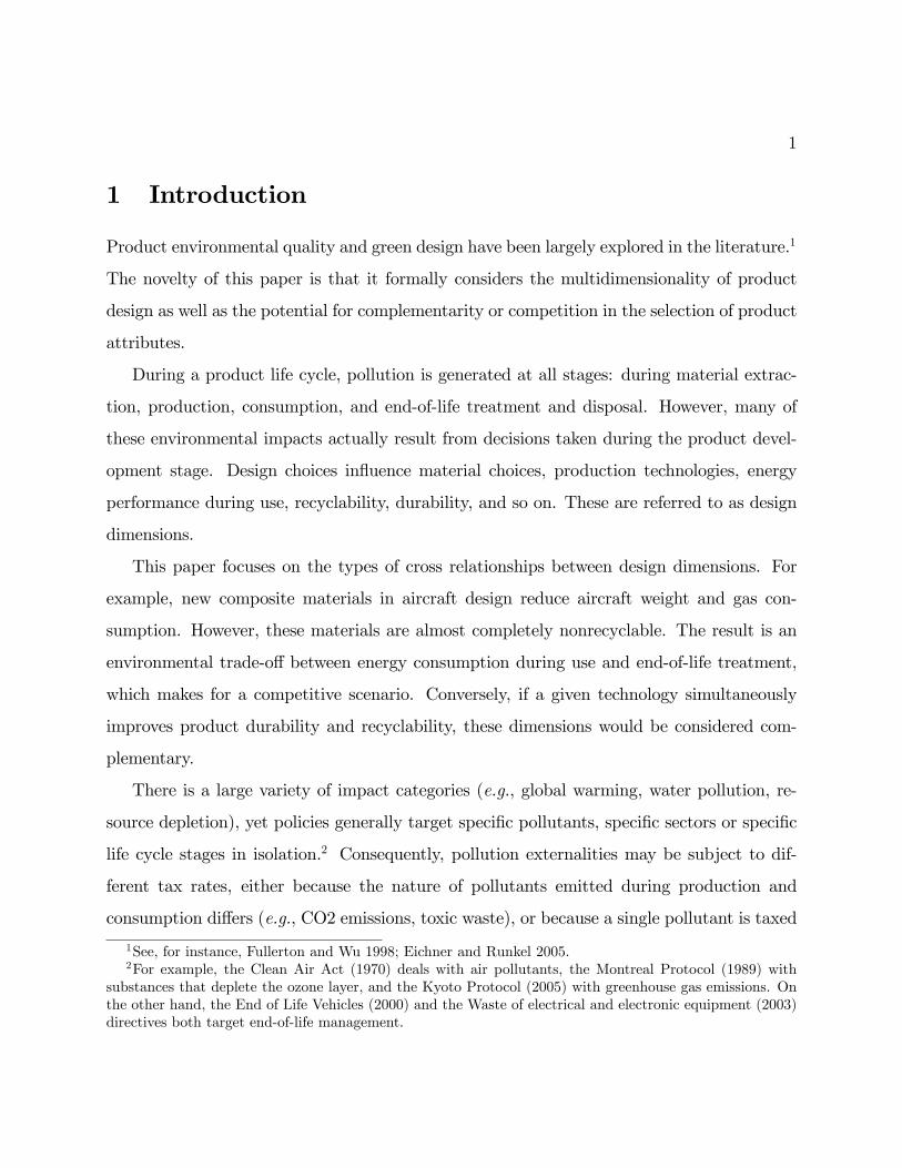
1 Introduction
Product environmental quality and green design have been largely explored in the literature.1
The novelty of this paper is that it formally considers the multidimensionality of product
design as well as the potential for complementarity or competition in the selection of product
attributes.
During a product life cycle, pollution is generated at all stages: during material extrac-
tion, production, consumption, and end-of-life treatment and disposal. However, many of
these environmental impacts actually result from decisions taken during the product devel-
opment stage. Design choices in�uence material choices, production technologies, energy
performance during use, recyclability, durability, and so on. These are referred to as design
dimensions.
This paper focuses on the types of cross relationships between design dimensions. For
example, new composite materials in aircraft design reduce aircraft weight and gas con-
sumption. However, these materials are almost completely nonrecyclable. The result is an
environmental trade-o¤ between energy consumption during use and end-of-life treatment,
which makes for a competitive scenario. Conversely, if a given technology simultaneously
improves product durability and recyclability, these dimensions would be considered com-
plementary.
There is a large variety of impact categories (e.g., global warming, water pollution, re-
source depletion), yet policies generally target speci�c pollutants, speci�c sectors or speci�c
life cycle stages in isolation.2 Consequently, pollution externalities may be subject to dif-
ferent tax rates, either because the nature of pollutants emitted during production and
consumption di¤ers (e.g., CO2 emissions, toxic waste), or because a single pollutant is taxed
1See, for instance, Fullerton and Wu 1998; Eichner and Runkel 2005.2For example, the Clean Air Act (1970) deals with air pollutants, the Montreal Protocol (1989) with
substances that deplete the ozone layer, and the Kyoto Protocol (2005) with greenhouse gas emissions. Onthe other hand, the End of Life Vehicles (2000) and the Waste of electrical and electronic equipment (2003)directives both target end-of-life management.
2
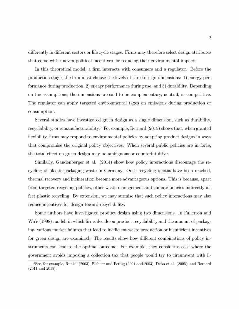
di¤erently in di¤erent sectors or life cycle stages. Firms may therefore select design attributes
that come with uneven political incentives for reducing their environmental impacts.
In this theoretical model, a �rm interacts with consumers and a regulator. Before the
production stage, the �rm must choose the levels of three design dimensions: 1) energy per-
formance during production, 2) energy performance during use, and 3) durability. Depending
on the assumptions, the dimensions are said to be complementary, neutral, or competitive.
The regulator can apply targeted environmental taxes on emissions during production or
consumption.
Several studies have investigated green design as a single dimension, such as durability,
recyclability, or remanufacturability.3 For example, Bernard (2015) shows that, when granted
�exibility, �rms may respond to environmental policies by adapting product designs in ways
that compromise the original policy objectives. When several public policies are in force,
the total e¤ect on green design may be ambiguous or counterintuitive.
Similarly, Gandenberger et al. (2014) show how policy interactions discourage the re-
cycling of plastic packaging waste in Germany. Once recycling quotas have been reached,
thermal recovery and incineration become more advantageous options. This is because, apart
from targeted recycling policies, other waste management and climate policies indirectly af-
fect plastic recycling. By extension, we may surmise that such policy interactions may also
reduce incentives for design toward recyclability.
Some authors have investigated product design using two dimensions. In Fullerton and
Wu�s (1998) model, in which �rms decide on product recyclability and the amount of packag-
ing, various market failures that lead to ine¢ cient waste production or insu¢ cient incentives
for green design are examined. The results show how di¤erent combinations of policy in-
struments can lead to the optimal outcome. For example, they consider a case where the
government avoids imposing a collection tax that people would try to circumvent with il-
3See, for example, Runkel (2003); Eichner and Pethig (2001 and 2003); Debo et al. (2005); and Bernard(2011 and 2015).

3
legal dumping. Applying a mixed policy that combines a packaging tax with recyclability
subsidies can also lead to the optimal social outcome. Although a pioneer in the �eld, their
study only considers two dimensions that show a neutral relationship.
Although Chen (2001), Eichner and Runkel (2003) and Subramanian et al. (2009) do not
formally de�ne cross relationships between dimensions, their implicit assumptions provide
interesting insights. Chen (2001) extends the multidimensionality of design attributes to
nonenvironmental dimensions. He proposes a scenario in which a �rm chooses the environ-
mental performance and a traditional attribute such as vehicle safety. His results indicate
that in order to prevent green customers from switching to a traditional product, the envi-
ronmental quality of the traditional product is decreased.
Eichner and Runkel (2003) argue that the use of thicker materials in product design
would not only improve durability, it would also facilitate product recuperation. In their
model, product weight correlates positively with both durability and recyclability. According
to our de�nitions, these dimensions would be considered complementary. This argument has
signi�cant implications for public policy making. For example, in a scenario where durability
is fully integrated in the market, market mechanisms will drive �rms to internalize consumer
preferences and choose optimal durability for their products. However, in the absence of a
market for recyclability, �rms will not choose optimal product recyclability. Consequently,
due to the complementarity between the two dimensions, the choice of durability would also
be inappropriate. Therefore, a public policy that encourages recycling could also restore
product durability to the optimal level.
Subramanian et al. (2009) examine design choices that a¤ect product environmental
performance during product use and product remanufacturability. Due to consumer hetero-
geneity, a trade-o¤ is made between the two dimensions, which therefore become competitive.
The "e¢ cient" consumer type is o¤ered a product with higher performance, which lowers
the usage cost such that the product is replaced less often. This results in lower disposal
costs, which in turn lowers the incentive for remanufacturability.
4
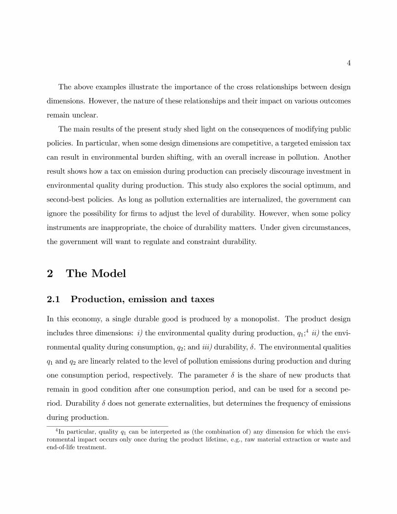
The above examples illustrate the importance of the cross relationships between design
dimensions. However, the nature of these relationships and their impact on various outcomes
remain unclear.
The main results of the present study shed light on the consequences of modifying public
policies. In particular, when some design dimensions are competitive, a targeted emission tax
can result in environmental burden shifting, with an overall increase in pollution. Another
result shows how a tax on emission during production can precisely discourage investment in
environmental quality during production. This study also explores the social optimum, and
second-best policies. As long as pollution externalities are internalized, the government can
ignore the possibility for �rms to adjust the level of durability. However, when some policy
instruments are inappropriate, the choice of durability matters. Under given circumstances,
the government will want to regulate and constraint durability.
2 The Model
2.1 Production, emission and taxes
In this economy, a single durable good is produced by a monopolist. The product design
includes three dimensions: i) the environmental quality during production, q1;4 ii) the envi-
ronmental quality during consumption, q2; and iii) durability, �. The environmental qualities
q1 and q2 are linearly related to the level of pollution emissions during production and during
one consumption period, respectively. The parameter � is the share of new products that
remain in good condition after one consumption period, and can be used for a second pe-
riod. Durability � does not generate externalities, but determines the frequency of emissions
during production.
4In particular, quality q1 can be interpreted as (the combination of) any dimension for which the envi-ronmental impact occurs only once during the product lifetime, e.g., raw material extraction or waste andend-of-life treatment.

5
Emissions ei(qi), for i = 1; 2, are such that e0i(qi) = �1. It is assumed that there is
no depreciation in the good�s quality when it lasts for two periods. Emission levels depend
strictly on the good�s qualities as selected at the production stage. The pollution generated
by one product over its lifetime is D = e1(q1) + (1 + ��)e2(q2), where � is a discount
factor. Because the product is useful for more than one period, it is said to provide 1 + ��
(discounted) functional units. Pollutant emissions can be expressed per functional unit as
follows:
Df =e1(q1)
(1 + ��)+ e2(q2):
The �rm�s unit production cost is c(q1;t; q2;t; �t) where c0(�) > 0, c00(�) > 0, and all the
cross derivatives follow the assumption made for the cost cross relationships between the three
dimensions. A positive (negative) cross derivative indicates a competitive (complementary)
relationship. For example, cq1� > 0 means that improving product durability raises the cost
of meeting a low-emission standard during production.
The social planner establishes a political platform where � 1 and � 2 are targeted environ-
mental taxes on emissions during production and during one consumption period, respec-
tively.
2.2 The demand and supply
An in�nitely lived representative household needs a given functionality or service supplied by
the produced good. For instance, the household needs one washing machine, one toaster, or
one vacuum cleaner. In this scenario, the parameter � represents the willingness to pay for
one consumption period, which is the corresponding welfare. At no time will the household
possess more than one of these goods.5 For instance, toasters sold at lower prices do not
5These assumptions allow us to focus the analysis on design choices and the corresponding pollutantemissions per unit of good. This avoids the time inconsistency problem, where �rms, in subsequent periods,
6
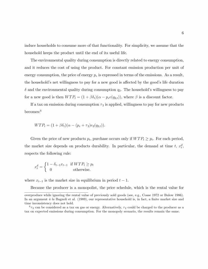
induce households to consume more of that functionality. For simplicity, we assume that the
household keeps the product until the end of its useful life.
The environmental quality during consumption is directly related to energy consumption,
and it reduces the cost of using the product. For constant emission production per unit of
energy consumption, the price of energy pe is expressed in terms of the emissions. As a result,
the household�s net willingness to pay for a new good is a¤ected by the good�s life duration
� and the environmental quality during consumption q2. The household�s willingness to pay
for a new good is then WTPt = (1 + ��t)(�� pee(q2;t)), where � is a discount factor.
If a tax on emission during consumption � 2 is applied, willingness to pay for new products
becomes:6
WTPt = (1 + ��t)(�� (pe + � 2)e2(q2;t)).
Given the price of new products pt, purchase occurs only if WTPt � pt. For each period,
the market size depends on products durability. In particular, the demand at time t, xdt ,
respects the following rule:
xdt =
�1� �t�1xt�1 if WTPt � pt0 otherwise.
where xt�1 is the market size in equilibrium in period t� 1.
Because the producer is a monopolist, the price schedule, which is the rental value for
overproduce while ignoring the rental value of previously sold goods (see, e.g., Coase 1972 or Bulow 1986).In an argument à la Bagnoli et al. (1989), our representative household is, in fact, a �nite market size andtime inconsistency does not hold.
6�2 can be considered as a tax on gas or energy. Alternatively, �2 could be charged to the producer as atax on expected emissions during consumption. For the monopoly scenario, the results remain the same.

7
the lifetime of each product, fully internalizes the consumer surplus:7
pt(q2;t; �t; � 2) = (1 + ��t)(�� (pe + � 2)e2(q2;t)):
With � being the producer�s pro�t, the supply function is such that:
xst =
�1� �t�1xt�1 if �(1� �t�1xt�1) � 0
0 otherwise.
In equilibrium, xdt = xst = xt, and it is assumed that �(1� �t�1xt�1) � 0 at all time so that
the market exists, i.e., xt = 1� �t�1xt�1 and pt(q2;t; �t; � 2) = (1 + ��t)(�� (pe + � 2)e2(q2;t)).
3 The equilibrium
The �rm�s intertemporal maximization problem is therefore:
maxfq1;t;q2;t;�t;xtg
V0 =TXt=0
�txt [p(q2;t; �t; � 2)� c(q1;t; q2;t; �t)� � 1e1(q1;t)]
s.t. xt+1 = 1� �txt (1)
x0 = x0 given
and where p(q2;t; �t; � 2) = (1 + ��t)(�� (pe + � 2)e2(q2;t));
where the state equation (1) can be written as xt+1 � xt = 1 � �txt � xt. To solve for the
dynamic problem, we use the Hamiltonian:
Ht = �txt [p(q2;t; �t; � 2)� c(q1;t; q2;t; �t)� � 1e1(q1;t)]+�t(1� �txt�xt) (t = 0; 1; :::; T )
7Bulow (1986) suggested that the monopolist could overcome the time inconsistency problem and increasepro�ts by renting the good instead of selling it. By assumption, we have that the monopolist will indi¤erentlysell or rent the good.
8
and the �rst order conditions are (for t = 0; 1; :::; T ):
@Ht
@q1;t= 0, �@c(q1;t; q2;t; �t)
@q1;t+ � 1 = 0
@Ht
@q2;t= 0, (1 + ��t)(pe + � 2)�
@c(q1;t; q2;t; �t)
@q2;t= 0
@Ht
@�t= 0, �txt
��(�� (pe + � 2)e2(q2;t))�
@c(q1;t; q2;t; �t)
@�t
�� �txt = 0
@Ht
@xt= �t�1 � �t , �t [p(q2;t; �t; � 2)� c(q1;t; q2;t; �t)� � 1e1(q1;t)]� �t�t � �t�1 = 0
@Ht
@�t= xt+1 � xt (t = 0; 1; :::; T � 1) :
In steady state, q1;t = q1;t+1 = q1; q2;t = q2;t+1 = q2; and �t = �t+1 = � 8t; and these
equilibrium conditions can be reduced to:
bq1(q1; q2; �; � 1) :) f1(q1; q2; �; � 1) = �@c(q1; q2; �)
@q1+ � 1 = 0 (2)
bq2(q1; q2; �; � 2) :) f2(q1; q2; �; � 2) = (1 + ��)(pe + � 2)�@c(q1; q2; �)
@q2= 0 (3)
b�(q1; q2; �; � 1) :)f�(q1; q2; �; � 1) = �
@c(q1; q2; �)
@�+
��
1 + ��
�[c(q1; q2; �) + � 1e1(q1)] = 0 (4)
and bx = 1
1 + b� : (5)
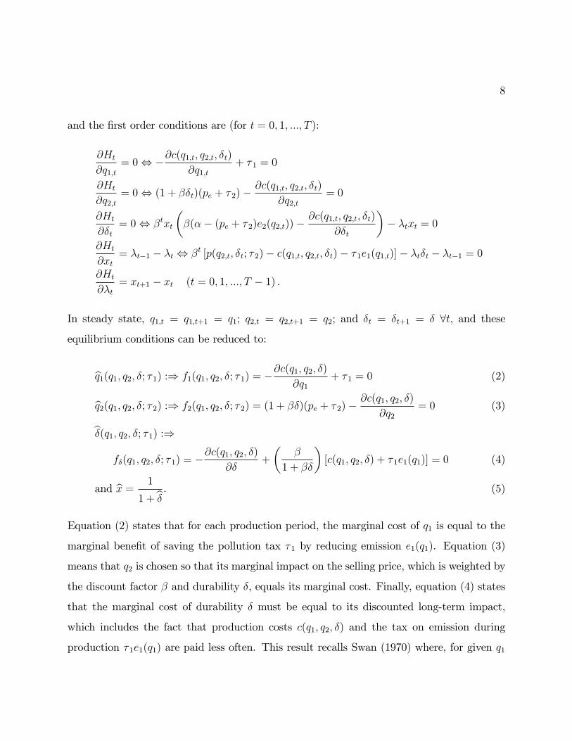
Equation (2) states that for each production period, the marginal cost of q1 is equal to the
marginal bene�t of saving the pollution tax � 1 by reducing emission e1(q1). Equation (3)
means that q2 is chosen so that its marginal impact on the selling price, which is weighted by
the discount factor � and durability �, equals its marginal cost. Finally, equation (4) states
that the marginal cost of durability � must be equal to its discounted long-term impact,
which includes the fact that production costs c(q1; q2; �) and the tax on emission during
production � 1e1(q1) are paid less often. This result recalls Swan (1970) where, for given q1
9
and q2, the choice of durability minimizes the cost of supplying a given functionality from a
stock of durable goods.
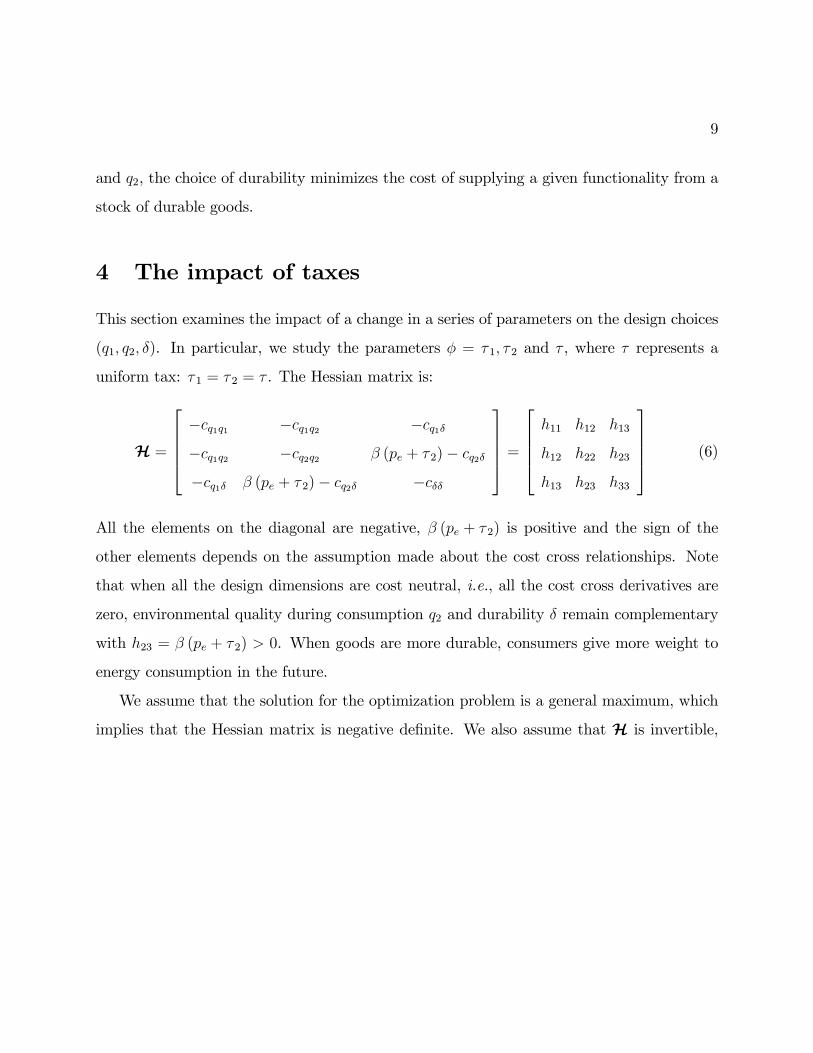
4 The impact of taxes
This section examines the impact of a change in a series of parameters on the design choices
(q1; q2; �). In particular, we study the parameters � = � 1; � 2 and � , where � represents a
uniform tax: � 1 = � 2 = � . The Hessian matrix is:
H =
26664�cq1q1 �cq1q2 �cq1��cq1q2 �cq2q2 � (pe + � 2)� cq2�
�cq1� � (pe + � 2)� cq2� �c��
37775 =26664h11 h12 h13
h12 h22 h23
h13 h23 h33
37775 (6)
All the elements on the diagonal are negative, � (pe + � 2) is positive and the sign of the
other elements depends on the assumption made about the cost cross relationships. Note
that when all the design dimensions are cost neutral, i.e., all the cost cross derivatives are
zero, environmental quality during consumption q2 and durability � remain complementary
with h23 = � (pe + � 2) > 0. When goods are more durable, consumers give more weight to
energy consumption in the future.
We assume that the solution for the optimization problem is a general maximum, which
implies that the Hessian matrix is negative de�nite. We also assume that H is invertible,
10
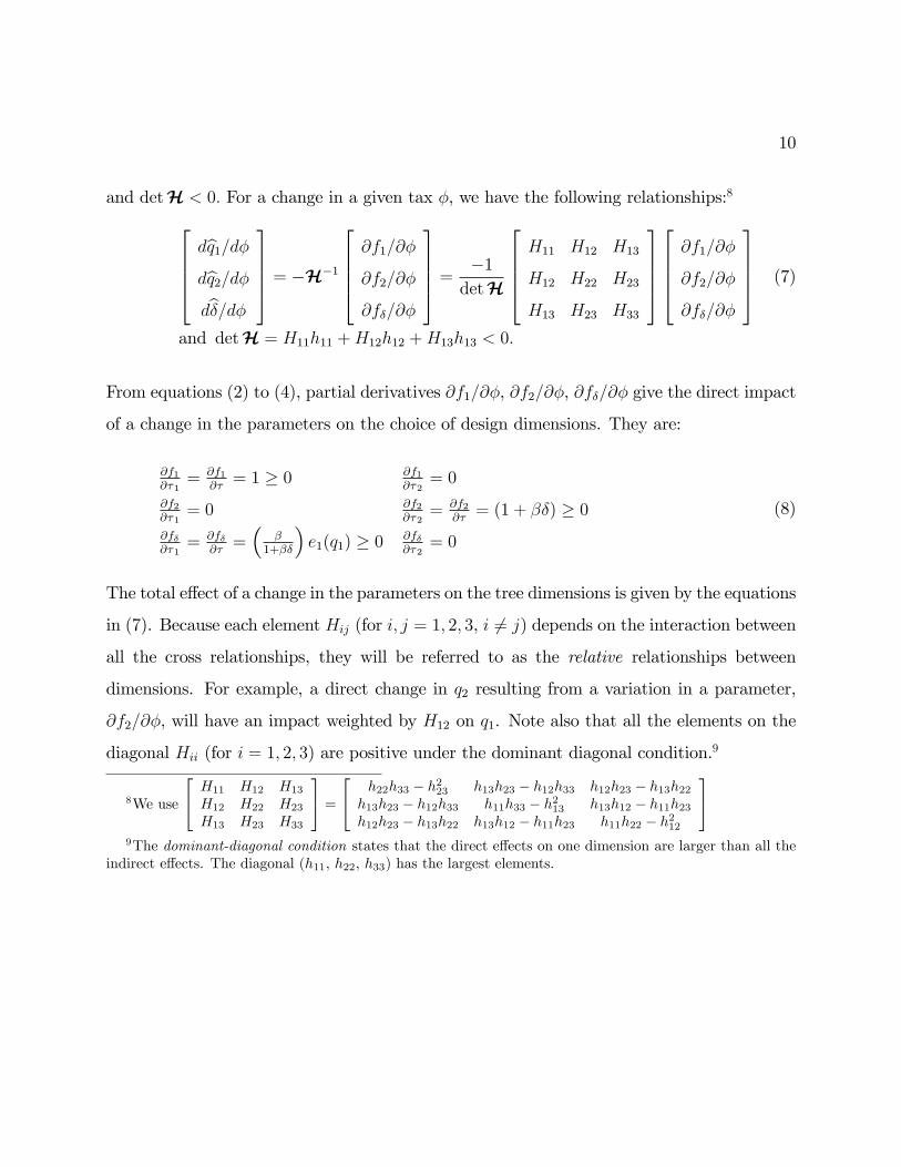
and detH < 0: For a change in a given tax �, we have the following relationships:826664dbq1=d�dbq2=d�db�=d�
37775 = �H�1
26664@f1=@�
@f2=@�
@f�=@�
37775 = �1detH
26664H11 H12 H13
H12 H22 H23
H13 H23 H33
3777526664@f1=@�
@f2=@�
@f�=@�
37775 (7)
and detH = H11h11 +H12h12 +H13h13 < 0:
From equations (2) to (4), partial derivatives @f1=@�, @f2=@�, @f�=@� give the direct impact
of a change in the parameters on the choice of design dimensions. They are:
@f1@�1
= @f1@�= 1 � 0 @f1
@�2= 0
@f2@�1
= 0 @f2@�2
= @f2@�= (1 + ��) � 0
@f�@�1
= @f�@�=�
�1+��
�e1(q1) � 0 @f�
@�2= 0
(8)
The total e¤ect of a change in the parameters on the tree dimensions is given by the equations
in (7). Because each element Hij (for i; j = 1; 2; 3, i 6= j) depends on the interaction between
all the cross relationships, they will be referred to as the relative relationships between
dimensions. For example, a direct change in q2 resulting from a variation in a parameter,
@f2=@�, will have an impact weighted by H12 on q1. Note also that all the elements on the
diagonal Hii (for i = 1; 2; 3) are positive under the dominant diagonal condition.9
8We use
24 H11 H12 H13H12 H22 H23H13 H23 H33
35 =24 h22h33 � h223 h13h23 � h12h33 h12h23 � h13h22h13h23 � h12h33 h11h33 � h213 h13h12 � h11h23h12h23 � h13h22 h13h12 � h11h23 h11h22 � h212
359The dominant-diagonal condition states that the direct e¤ects on one dimension are larger than all the
indirect e¤ects. The diagonal (h11, h22, h33) has the largest elements.
11
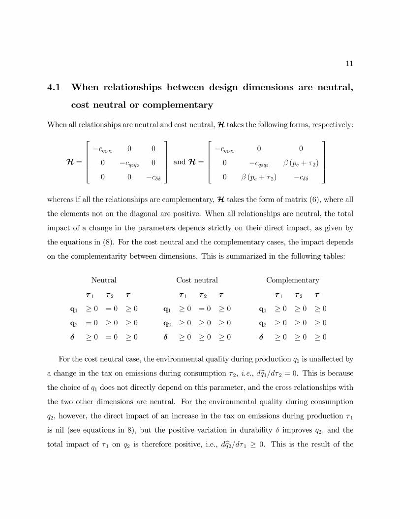
4.1 When relationships between design dimensions are neutral,
cost neutral or complementary
When all relationships are neutral and cost neutral,H takes the following forms, respectively:
H =
26664�cq1q1 0 0
0 �cq2q2 0
0 0 �c��
37775 and H =
26664�cq1q1 0 0
0 �cq2q2 � (pe + � 2)
0 � (pe + � 2) �c��
37775whereas if all the relationships are complementary,H takes the form of matrix (6), where all
the elements not on the diagonal are positive. When all relationships are neutral, the total
impact of a change in the parameters depends strictly on their direct impact, as given by
the equations in (8). For the cost neutral and the complementary cases, the impact depends
on the complementarity between dimensions. This is summarized in the following tables:
Neutral
� 1 � 2 �
q1 � 0 = 0 � 0
q2 = 0 � 0 � 0
� � 0 = 0 � 0
Cost neutral
� 1 � 2 �
q1 � 0 = 0 � 0
q2 � 0 � 0 � 0
� � 0 � 0 � 0
Complementary
� 1 � 2 �
q1 � 0 � 0 � 0
q2 � 0 � 0 � 0
� � 0 � 0 � 0
For the cost neutral case, the environmental quality during production q1 is una¤ected by
a change in the tax on emissions during consumption � 2, i.e., dbq1=d� 2 = 0. This is becausethe choice of q1 does not directly depend on this parameter, and the cross relationships with
the two other dimensions are neutral. For the environmental quality during consumption
q2, however, the direct impact of an increase in the tax on emissions during production � 1
is nil (see equations in 8), but the positive variation in durability � improves q2, and the
total impact of � 1 on q2 is therefore positive, i.e., dbq2=d� 1 � 0. This is the result of the

12
complementarity between the environmental quality during consumption q2 and durability
�, which also induces the positive e¤ect of a tax on emissions during consumption � 2 on
durability �, or db�=d� 2 > 0.Proposition 1 When the relationships between design dimensions q1, q2 and � are all neu-
tral or complementary,
� an increase in the tax on emissions during production � 1 or during consumption � 2,
or an increase in a uniform tax � always improve green design and reduces pollution
emissions per functional unit Df .
4.2 When some relationships between design dimensions are com-
petitive
The impact of a change in the tax on emission during production and consumption, � 1 and
� 2, are respectively:
dbq1d�1= �1
detH
�H11 +H13
��
1+��
�e1(q1)
�Q 0; dbq1
d�2= �1
detHH12(1 + ��) Q 0dbq2d�1= �1
detH
�H12 +H23
��
1+��
�e1(q1)
�Q 0; dbq2
d�2= �1
detHH22(1 + ��) > 0
db�d�1= �1
detH
�H13 +H33
��
1+��
�e1(q1)
�Q 0; db�
d�2= �1
detHH23(1 + ��) Q 0
Which gives us the following proposition.
Proposition 2 When some of the relationships between design dimensions q1, q2 and �
are competitive, the full impact of a change depend on the relative relationships between
dimensions.
� A change in the tax on emission during production � 1 has ambiguous e¤ects on the
three dimensions.
13
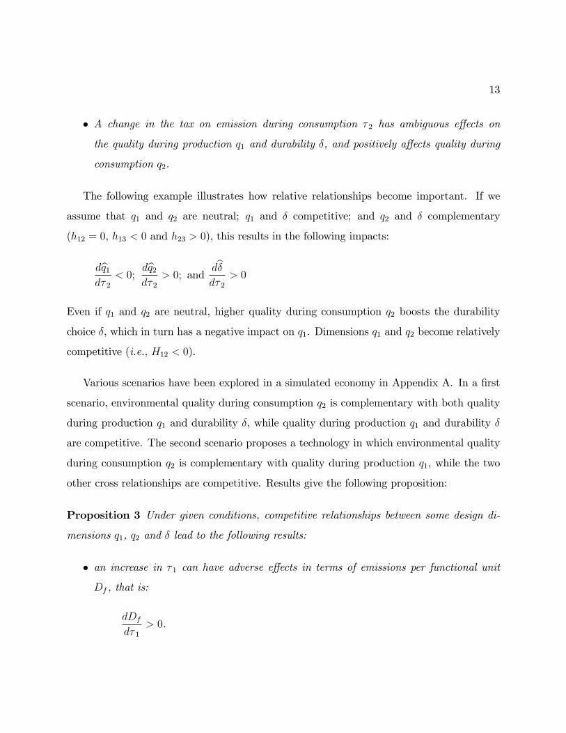
� A change in the tax on emission during consumption � 2 has ambiguous e¤ects on
the quality during production q1 and durability �, and positively a¤ects quality during
consumption q2.
The following example illustrates how relative relationships become important. If we
assume that q1 and q2 are neutral; q1 and � competitive; and q2 and � complementary
(h12 = 0, h13 < 0 and h23 > 0), this results in the following impacts:
dbq1d� 2
< 0;dbq2d� 2
> 0; anddb�d� 2
> 0
Even if q1 and q2 are neutral, higher quality during consumption q2 boosts the durability
choice �, which in turn has a negative impact on q1. Dimensions q1 and q2 become relatively
competitive (i.e., H12 < 0).
Various scenarios have been explored in a simulated economy in Appendix A. In a �rst
scenario, environmental quality during consumption q2 is complementary with both quality
during production q1 and durability �, while quality during production q1 and durability �
are competitive. The second scenario proposes a technology in which environmental quality
during consumption q2 is complementary with quality during production q1, while the two
other cross relationships are competitive. Results give the following proposition:
Proposition 3 Under given conditions, competitive relationships between some design di-
mensions q1, q2 and � lead to the following results:
� an increase in � 1 can have adverse e¤ects in terms of emissions per functional unit
Df , that is:
dDf
d� 1> 0.
14
� an increase in the tax on emissions during production � 1 can reduce the environmental
quality of the good during production q1, causing therefore an increase in emissions
during production e1, that is:
dbq1d� 1
< 0 andde1(q1)
d� 1> 0.
Proposition 3 says that a targeted tax on emissions during production possibly leads to
an increase in the overall emissions, or an increase in the targeted pollutant per unit of good.
While aiming for lower emissions of a speci�c pollutant, an environmental policy may have
adverse e¤ects.
5 Optimal policies
5.1 Social optimum
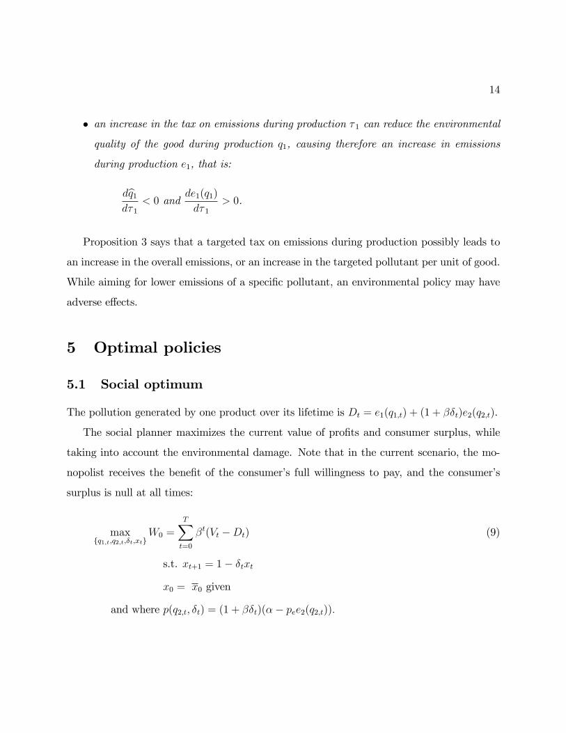
The pollution generated by one product over its lifetime is Dt = e1(q1;t) + (1 + ��t)e2(q2;t).
The social planner maximizes the current value of pro�ts and consumer surplus, while
taking into account the environmental damage. Note that in the current scenario, the mo-
nopolist receives the bene�t of the consumer�s full willingness to pay, and the consumer�s
surplus is null at all times:
maxfq1;t;q2;t;�t;xtg
W0 =
TXt=0
�t(Vt �Dt) (9)
s.t. xt+1 = 1� �txt
x0 = x0 given
and where p(q2;t; �t) = (1 + ��t)(�� pee2(q2;t)):
15
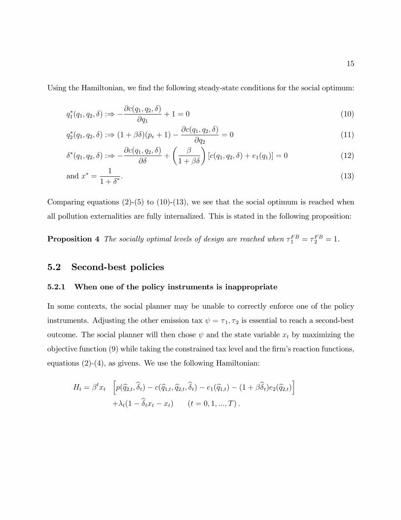
Using the Hamiltonian, we �nd the following steady-state conditions for the social optimum:
q�1(q1; q2; �) :) �@c(q1; q2; �)@q1
+ 1 = 0 (10)
q�2(q1; q2; �) :) (1 + ��)(pe + 1)�@c(q1; q2; �)
@q2= 0 (11)
��(q1; q2; �) :) �@c(q1; q2; �)@�
+
��
1 + ��
�[c(q1; q2; �) + e1(q1)] = 0 (12)
and x� =1
1 + ��: (13)
Comparing equations (2)-(5) to (10)-(13), we see that the social optimum is reached when
all pollution externalities are fully internalized. This is stated in the following proposition:
Proposition 4 The socially optimal levels of design are reached when �FB1 = �FB2 = 1.
5.2 Second-best policies
5.2.1 When one of the policy instruments is inappropriate
In some contexts, the social planner may be unable to correctly enforce one of the policy
instruments. Adjusting the other emission tax = � 1; � 2 is essential to reach a second-best
outcome. The social planner will then chose and the state variable xt by maximizing the
objective function (9) while taking the constrained tax level and the �rm�s reaction functions,
equations (2)-(4), as givens. We use the following Hamiltonian:
Ht = �txt
hp(bq2;t;b�t)� c(bq1;t; bq2;t;b�t)� e1(bq1;t)� (1 + �b�t)e2(bq2;t)i+�t(1� b�txt � xt) (t = 0; 1; :::; T ) :

16
In steady state, we have (see Appendix B.1 for details):��@c(q1; q2; �)
@q1+ 1
�dbq1d
+
�(1 + ��)pe �
@c(q1; q2; �)
@q2+ (1 + ��)
�dbq2d
���
1 + ��(�c(q1; q2; �)� e1(q1)) +
@c(q1; q2; �)
@�
�db�d
= 0 (14)
Scenario � 1 = � 1: the government faces a political constraint on the tax on emissions
during production � 1 = � 1 and chooses = � 2. Using (14) and the �rm�s reaction functions
(2)-(4), the optimal tax on emissions during consumption �SB2 for any given � 1 is such that:
�SB2 :) (1� � 1)dbq1d� 2
+ (1� �SB2 )(1 + ��)dbq2d� 2
+ (1� � 1)�
1 + ��(e1(q1))
db�d� 2
= 0
which can be rewritten as
�SB2 :) (1 + ��) (1� �SB2 ) + (1� � 1)
�H12
H22
+�
1 + ��e1(q1)
H23
H22
�= 0 (15)
where the relative relationships H12 and H23 also depend on the selected tax on emission
during consumption �SB2 . Using equation (15)�s �rst derivative, comparative static tells us
that
signd�SB2d� 1
= sign
�(1� �SB2 )
db�d� 1
��H12
H22
+�
1 + ��e1(q1)
H23
H22
�
�(1� � 1)
��
1 + ��
�2e1(q1)
db�d� 1
+�
1 + ��
dbq1d� 1
!H23
H22
!
When evaluated at � 1 = �FB1 = 1, and knowing that �SB2 (� 1 = �FB1 ) = 1, we have that
signd�SB2d� 1
�����1=1
= �sign�H12 +
�
1 + ��e1(q1)H23
�:
Scenario � 2 = � 2: the government faces a political constraint on the tax on emissions
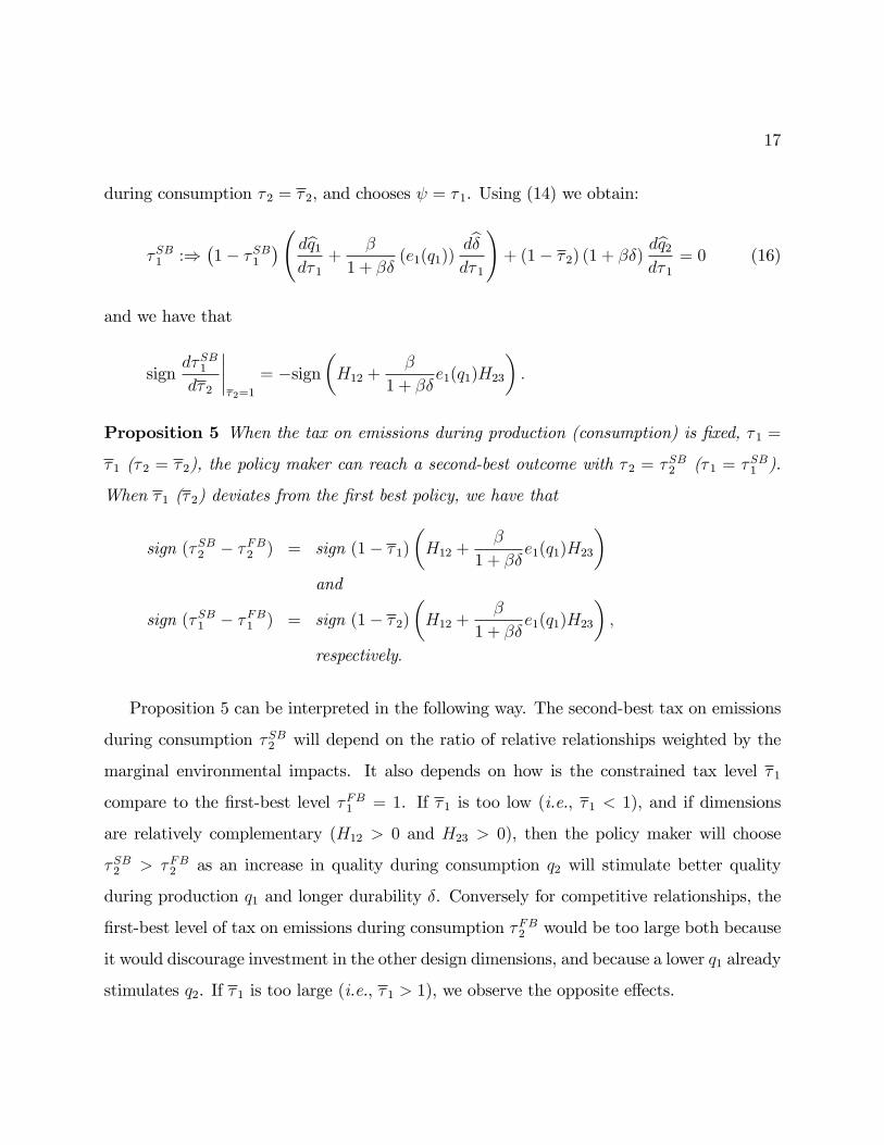
17
during consumption � 2 = � 2, and chooses = � 1. Using (14) we obtain:
�SB1 :)�1� �SB1
� dbq1d� 1
+�
1 + ��(e1(q1))
db�d� 1
!+ (1� � 2) (1 + ��)
dbq2d� 1
= 0 (16)
and we have that
signd�SB1d� 2
�����2=1
= �sign�H12 +
�
1 + ��e1(q1)H23
�:
Proposition 5 When the tax on emissions during production (consumption) is �xed, � 1 =
� 1 (� 2 = � 2), the policy maker can reach a second-best outcome with � 2 = �SB2 (� 1 = �SB1 ).
When � 1 (� 2) deviates from the �rst best policy, we have that
sign (�SB2 � �FB2 ) = sign (1� � 1)
�H12 +
�
1 + ��e1(q1)H23
�and
sign (�SB1 � �FB1 ) = sign (1� � 2)
�H12 +
�
1 + ��e1(q1)H23
�;
respectively:
Proposition 5 can be interpreted in the following way. The second-best tax on emissions
during consumption �SB2 will depend on the ratio of relative relationships weighted by the
marginal environmental impacts. It also depends on how is the constrained tax level � 1
compare to the �rst-best level �FB1 = 1. If � 1 is too low (i.e., � 1 < 1), and if dimensions
are relatively complementary (H12 > 0 and H23 > 0), then the policy maker will choose
�SB2 > �FB2 as an increase in quality during consumption q2 will stimulate better quality
during production q1 and longer durability �. Conversely for competitive relationships, the
�rst-best level of tax on emissions during consumption �FB2 would be too large both because
it would discourage investment in the other design dimensions, and because a lower q1 already
stimulates q2. If � 1 is too large (i.e., � 1 > 1), we observe the opposite e¤ects.
18
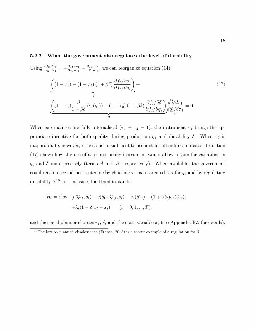
5.2.2 When the government also regulates the level of durability
Using @f2@q2
dbq2d�1= �@f2
@q1
dbq1d�1� @f2
@�df�d�1, we can reorganize equation (14):�
(1� � 1)� (1� � 2) (1 + ��)@f2=@q1@f2=@q2
�| {z }
A
+ (17)
�(1� � 1)
�
1 + ��(e1(q1))� (1� � 2) (1 + ��)
@f2=@�
@f2=@q2
�| {z }
B
db�=d� 1dbq1=d� 1
C
= 0
When externalities are fully internalized (� 1 = � 2 = 1), the instrument � 1 brings the ap-
propriate incentive for both quality during production q1 and durability �. When � 2 is
inappropriate, however, � 1 becomes insu¢ cient to account for all indirect impacts. Equation
(17) shows how the use of a second policy instrument would allow to aim for variations in
q1 and � more precisely (terms A and B, respectively). When available, the government
could reach a second-best outcome by choosing � 1 as a targeted tax for q1 and by regulating
durability �.10 In that case, the Hamiltonian is:
Ht = �txt [p(bq2;t; �t)� c(bq1;t; bq2;t; �t)� e1(bq1;t)� (1 + ��t)e2(bq2;t)]+�t(1� �txt � xt) (t = 0; 1; :::; T ) :
and the social planner chooses � 1, �t and the state variable xt (see Appendix B.2 for details).
10The law on planned obsolescence (France, 2015) is a recent example of a regulation for �.
19
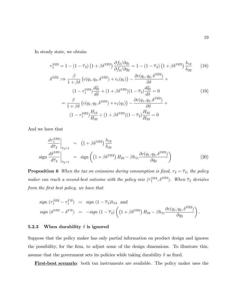
In steady state, we obtain:
�SB21 = 1� (1� � 2)�1 + ��SB2
� @f2=@q1@f2=@q2
= 1� (1� � 2)�1 + ��SB2
� h12h22
(18)
�SB2 :) �
1 + ��
�c(q1; q2; �
SB2) + e1(q1)�� @c(q1; q2; �
SB2)
@�+
(1� �SB21 )dbq1d�+ (1 + ��SB2)(1� � 2)
dbq2d�
= 0 (19)
=�
1 + ��
�c(q1; q2; �
SB2) + e1(q1)�� @c(q1; q2; �
SB2)
@�+
(1� �SB21 )H13
H33
+ (1 + ��SB2)(1� � 2)H23
H33
= 0
And we have that
d�SB21
d� 2
�����2=1
=�1 + ��SB2
� h12h22
signd�SB2
d� 2
�����2=1
= sign��1 + ��SB2
�H23 � �h11
@c(q1; q2; �SB2)
@q2
�(20)
Proposition 6 When the tax on emissions during consumption is �xed, � 2 = � 2, the policy
maker can reach a second-best outcome with the policy mix (�SB21 ; �SB2). When � 2 deviates
from the �rst best policy, we have that
sign (�SB21 � �FB1 ) = sign (1� � 2)h12 and
sign (�SB2 � �FB) = �sign (1� � 2)
��1 + ��SB2
�H23 � �h11
@c(q1; q2; �SB2)
@q2
�:
5.2.3 When durability � is ignored
Suppose that the policy maker has only partial information on product design and ignores
the possibility, for the �rm, to adjust some of the design dimensions. To illustrate this,
assume that the government sets its policies while taking durability � as �xed.
First-best scenario: both tax instruments are available. The policy maker uses the

20
optimality conditions for q1 and q2 (10) and (11), takes into account the �rm�s responses (2)
and (3), but ignores the choice of durability (4). The government sets � 1 = � 2 = �FB1 = �FB2 ,
and obtains the �rst-best outcome. When all externalities are internalized, incentives are in
place for the optimal choice of durability as well.
Scenario � 2 = � 2: the social planner uses the second-best strategy described by equation
(18) and sets e�SB1 . Then the �rm chooses the level of durability e�SB according to equation(4): e�SB = b�(e�SB1 ).
We have that
e�SB1 = 1� (1� � 2)�1 + �e�SB� @f2=@q1
@f2=@q2= 1� (1� � 2)
�1 + �e�SB� h12
h22(21)
e�SB :) �
1 + �e�SB!h
c(q1; q2;e�SB) + e�SB1 e1(q1)i� @c(q1; q2;e�SB)
@�= 0 (22)
and, using H22 = h11h33 � h213,
d e� 1SBd� 2
������2=1
=�1 + �e�SB� h12
h22
signde�SBd� 2
������2=1
= sign
�h33
�1 + �e�SB�H23 + �H22
@c(q1; q2;e�SB)@q2
!(23)
= sign
�1 + �e�SB�H23 � �h11
@c(q1; q2;e�SB)@q2
+ �h213h33
@c(q1; q2;e�SB)@q2
!:
When comparing the equilibrium conditions (18), (19), and (21), (22), we see that if the
tax on emissions during consumption is constrained to the �rst best value � 2 = �FB2 = 1,
the selected tax on emission during production will also be optimal whether or not the
government regulates the level of durability �SB21 = e�SB1 = �FB1 = 1. This results in the �rst
best level of durability �SB2 = e�SB = ��. Equations (20) and (23) describes what occurs
when the tax on emissions during consumption deviates from the �rst best value. This leads
to the following result:
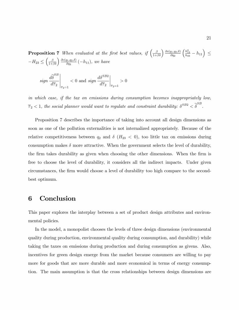
21
Proposition 7 When evaluated at the �rst best values, if�
�1+��
�@c(q1;q2;�)
@q2
�h213h33� h11
��
�H23 ��
�1+��
�@c(q1;q2;�)
@q2(�h11), we have
signde�SBd� 2
������2=1
< 0 and signd�SB2
d� 2
�����2=1
> 0
in which case, if the tax on emissions during consumption becomes inappropriately low,
� 2 < 1, the social planner would want to regulate and constraint durability: �SB2 < e�SB.
Proposition 7 describes the importance of taking into account all design dimensions as
soon as one of the pollution externalities is not internalized appropriately. Because of the
relative competitiveness between q2 and � (H23 < 0), too little tax on emissions during
consumption makes � more attractive. When the government selects the level of durability,
the �rm takes durability as given when choosing the other dimensions. When the �rm is
free to choose the level of durability, it considers all the indirect impacts. Under given
circumstances, the �rm would choose a level of durability too high compare to the second-
best optimum.
6 Conclusion
This paper explores the interplay between a set of product design attributes and environ-
mental policies.
In the model, a monopolist chooses the levels of three design dimensions (environmental
quality during production, environmental quality during consumption, and durability) while
taking the taxes on emissions during production and during consumption as givens. Also,
incentives for green design emerge from the market because consumers are willing to pay
more for goods that are more durable and more economical in terms of energy consump-
tion. The main assumption is that the cross relationships between design dimensions are
22
complementary, neutral, or competitive.
The impact of changes in tax policies was examined. When all design dimensions are
complementary or neutral, tax increases always spur greener design and reduce emissions.
However, when some design dimensions are competitive, the adverse e¤ects may occur when
a more stringent environmental tax induces the production of more polluting goods.
The social optimal taxation level implies a uniform tax on emissions during both pro-
duction and consumption. Any deviation from the optimal tax levels can impact all three
dimensions, with adverse environmental consequences. Second-best policies must take into
account crossed e¤ects.
To conclude, targeted environmental policies should take into account �rms�responses
in terms of product design, especially when design dimensions show competitive cross rela-
tionships.
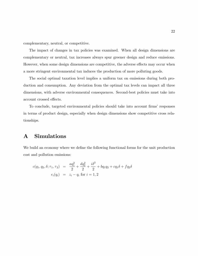
A Simulations
We build an economy where we de�ne the following functional forms for the unit production
cost and pollution emissions:
c(q1; q2; �; � 1; � 2) =aq212+dq222+i�2
2+ bq1q2 + cq1� + fq2�
ei(qi) = zi � qi for i = 1; 2
23
where the signs of b, c and f denote the cost cross relationship between the dimensions. The
Hessian matrix becomes:
H =
26664�cq1q1 �cq1q2 �cq1��cq1q2 �cq2q2 � (pe + � 2)� cq2�
�cq1� � (pe + � 2)� cq2� �c��
37775 =26664h11 < 0 h12 h13
h12 h22 < 0 h23
h13 h23 h33 < 0
37775 =26664�a �b �c
�b �d � (pe + � 2)� f
�c � (pe + � 2)� f �i
37775Note that optimality conditions for the choice of design, equations (2) to (4) can be
rewritten as:
bq1(�; � 1; � 2) = 1
H33
[d� 1 � b(pe + � 2) +H13�]
bq2(�; � 1; � 2) = 1
H33
[a(pe + � 2)� b� 1 +H23�]
b�(q1; q2; �; � 1; � 2)) �
�aq212+dq222� i�2
2+ bq1q2 + � 1(z1 � q1)
�� (i� + cq1 + fq2) = 0
which highlight the role of H13 and H23 in in�uencing the impact of � on q1 and q2, respec-
tively.
We assign the parameters the following values:
a = 5; d = i = 6; b = �1; f = �:5; and c = 4:5
which means that environmental quality during consumption q2 is complementary with both
quality during production q1 and durability �, whereas quality during production q1 and
24
durability � are competitive. Other parameters take the values:
� = :97; pe = 2:4; z1 = 1:8; z2 = 2:5 and � 2 = 1.
We obtain interior solutions for � 1 2 [8:3; 9]. The Hessian matrix is negative de�nite. In
the range of interior solutions, an increase in the targeted tax � 1 favors q1 and brings a
simultaneous reduction in q2 and �. The overall result is that for lower values of � 1, i.e., for
� 1 2 [8:3; 8:7], a tax increase increases the level of emission per functional unit Df . This is
illustrated in Figure 1.
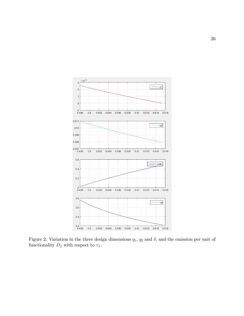
Figure 2 shows the results using the following set of parameters:
a = 1; 730; d = 6:69; i = :10; b = �8; f = 3:30; and c = 9:49
� = :97; pe = 2:4; z1 = 1:8; z2 = 2:5 and � 2 = 1,
which assume that environmental quality during consumption q2 is complementary with
quality during production q1, and that the other cross relationships are competitive. We
see that an increase in the targeted tax on pollution during production � 1 makes products
design more polluting during the production stage, i.e., q1 decreases.

25
Figure 1: Variation in the three design dimensions q1, q2 and �; and the emissions per unitof functionality Df with respect to � 1:
26
Figure 2: Variation in the three design dimensions q1, q2 and �; and the emission per unit offunctionality Df with respect to � 1:

27
B Second-best policies
B.1 When one of the policy instruments is inappropriate
The optimality conditions are (for t = 1; :::; T ):
@Ht
@ t= 0, �txt
���@c(q1;t; q2;t; �t)
@q1;t+ 1
�dbq1;td t
+�(1 + ��t)pe �
@c(q1;t; q2;t; �t)
@q2;t+ (1 + ��t)
�dbq2;td t
+��(�� pee2(q2;t))�
@c(q1;t; q2;t; �t)
@�t� �e2(q2;t)
�db�td t
#� �txt
db�td t
= 0
@Ht
@xt= �t�1 � �t , �t [p(q2;t; �t)� c(q1;t; q2;t; �t)� e1(q1;t)� (1 + ��t)e2(q2;t)]
� �t�t � �t�1 = 0
@Ht
@�t= xt+1 � xt t = 0; 1; :::; T � 1:
B.2 Scenario � 2 = � 2
When � 2 = � 2 and the government chooses � 1, �t, the �rm must take durability as given and
equation (4) is no longer applicable. The Hessian matrix (6) becomesH =
24 �cq1q1 �cq1q2�cq1q2 �cq2q2
35 =24 h11 h12
h12 h22
35 and the full impact of a change in a parameter (7) is24 dbq1=d�dbq2=d�
35 = �H�1
24 @f1=@�
@f2=@�
35 = �1detH
24 h22 �h12�h12 h11
3524 @f1=@�
@f2=@�
35and detH = h11h22 � h212 = H33 > 0:
28
The optimality conditions are (for t = 1; :::; T ):
@Ht
@� 1= 0,
��@c(q1;t; q2;t; �t)
@q1;t+ 1
�dbq1;td� 1
+�(1 + ��)pe �
@c(q1;t; q2;t; �t)
@q2;t+ (1 + ��t)
�dbq2;td� 1
= 0
@Ht
@�t= �txt
���(�� pee2(q2;t))�
@c(q1;t; q2;t; �t)
@�t� �e2(q2;t)
��� �txt+
@Ht
@q1;t
dbq1;td�t
+@Ht
@q2;t
dbq2;td�t
= 0
@Ht
@xt= �t�1 � �t , �t [p(q2;t; �t)� c(q1;t; q2;t; �t)� e1(q1;t)� (1 + ��t)e2(q2;t)]
� �t� � �t�1 = 0
@Ht
@�t= xt+1 � xt t = 0; 1; :::; T � 1:
and we use the following properties:
@f1@�
= �cq1� = h13
@f2@�
= �(pe + � 2)� cq2� = h23
dbq1d�
=�1detH(h22h13 � h12h23) =
H13
H33
dbq2d�
=�1detH(�h12h13 + h11h23) =
H23
H33
References
Bagnoli, Mark, Stephen W. Salant, and Joseph E. Swierzbinski (1989) �Durable-goodsmonopoly with discrete demand.�The Journal of Political Economy 97 (6), 1459�1478
Bernard, Sophie (2011) �Remanufacturing.�Journal of Environmental Economics and Man-agement 62, 337�351
(2015) �North-South trade in reusable goods: green design meets illegal shipments ofwaste.�Journal of Environmental Economics and Management 69, 22�35

29
Bulow, Jeremy (1986) �An economic theory of planned obsolescence.�The Quaterly Journalof Economics 101, 729�750
Chen, Chialin (2001) �Design for the environment: A quality-based model for green productdevelopment.�Management Science 47, 250�263
Coase, Ronald H. (1972) �Durability and monopoly.� Jounal of Law and Economics 15(1), 143�149
Debo, Laurens G., L. Beril Toktay, and Luk N. VanWassenhove (2005) �Market segmentationand product technology selection for remanufacturable products.�Management Science51, 1193�1205
Eichner, Thomas, and Marco Runkel (2003) �E¢ cient management of product durability andrecyclability under utilitarian and chichilnisky preferences.�Journal of Economics Vol.80, No. 1, 43�75
Eichner, Thomas, and Marco Runkel (2005) �E¢ cient policies for green design in a vintagedurable good model.�Environmental and Resource Economics (2005) 30, 259�278
Eichner, Thomas, and Rudiger Pethig (2001) �Product design and e¢ cient management ofrecycling and waste treatment.�Journal of Environmental Economics and Management41, 109�134
Eichner, Thomas, and Rüdiger Pethig (2003) �Corrective taxation for curbing pollution andpromoting green product design and recycling.�Environmental and Resource Economics25, 477�500
Fullerton, Don, and Wenbo Wu (1998) �Policies for green design.�Journal of EnvironmentalEconomics and Management 36, 131�148
Gandenberger, Carsten, Robert Orzanna, Sara KlingenfuSS, and Christian Sartorius (2014)�The impact of policy interactions on the recycling of plastic packaging waste in ger-many.�Technical Report Working Paper Sustainability and Innovation No. S8/2014,Econstor
Runkel, Marco (2003) �Product durability and extended producer responsibility in solid wastemanagement.�Environmental and Resource Economics 24, 161�182
Subramanian, Ravi, Sudheer Gupta, and Brian Talbot (2009) �Product design and supplychain coordination under extended producer responsibility.�Production and OperationsManagement 18, 259�277

30
Swan, Peter L. (1970) �Durability of consumption goods.�American Economic Review 60(5), 884�894
Related Documents


