Design and Simulation of Unified Power Flow Controller with Grid Storage by Christopher Beaudoin A Thesis submitted to the Faculty of Graduate Studies of The University of Manitoba in partial fulfilment of the requirements of the degree of MASTER OF SCIENCE Department of Electrical and Computer Engineering University of Manitoba Winnipeg Copyright 2021 Christopher Beaudoin

Welcome message from author
This document is posted to help you gain knowledge. Please leave a comment to let me know what you think about it! Share it to your friends and learn new things together.
Transcript

Design and Simulation of Unified Power Flow Controller with Grid Storage
by
Christopher Beaudoin
A Thesis submitted to the Faculty of Graduate Studies of
The University of Manitoba
in partial fulfilment of the requirements of the degree of
MASTER OF SCIENCE
Department of Electrical and Computer Engineering
University of Manitoba
Winnipeg
Copyright © 2021 Christopher Beaudoin

Abstract
Power flow between two transmission systems across an uncontrolled interface can be problematic
if there is unequal sharing between the tie lines. System configuration changes such as generation
dispatch, or out of service elements can cause thermal overloads. In addition, some weaker areas
of the system which may have insufficient transmission can have difficultly supporting the voltage
at buses with high loading particularly after the loss of one element.
This thesis presents a real transmission system which has two problems: a thermal limitation
caused by unequal tie-sharing across an uncontrolled interface, and a post-fault voltage stability
concern. Various potential solutions are analyzed and shown to address one or the other of these two
problems; none of which were capable of solving both. A Unified Power Flow Controller (UPFC)
is proposed which can effectively address both problems and can provide additional benefit in the
form of a grid storage interface.
The operational characteristics of a UPFC are analyzed and used to develop an electrical model
and control system topology. The model with its control system is implemented in PSCAD. The
UPFC is proven to be capable of effectively addressing the thermal limitation and voltage stability
issues of the system. Further, a battery is added to the UPFC to provide grid energy storage. Cost
saving measures through controller design are also proposed and implemented.
This work demonstrates that a UPFC can be an effective solution to typical problems (such as
thermal and voltage constraints) faced by a transmission system. A UPFC with grid storage can also
- ii -

provide an alternative to building costly transmission lines or generation by enhancing reliability,
reducing demand on generation cause by system peaks, smoothing intermittent generation, etc.
- iii -

Acknowledgments
I want to thank Dr. Filizadeh who has provide direction and assistance throughout the process of
completing this program. Also, I want to thank Manitoba Hydro for providing financial assistance,
simulation software, and modeling data, all of which were instrumental for the completion of this
program.
- iv -

TABLE OF CONTENTS
Table of Contents
Abstract . . . . . . . . . . . . . . . . . . . . . . . . . . . . . . . . . . . . . . . . . . . . . . ii
Acknowledgments . . . . . . . . . . . . . . . . . . . . . . . . . . . . . . . . . . . . . . . . . iv
Table of Contents . . . . . . . . . . . . . . . . . . . . . . . . . . . . . . . . . . . . . . . . . v
List of Figures . . . . . . . . . . . . . . . . . . . . . . . . . . . . . . . . . . . . . . . . . . ix
List of Tables . . . . . . . . . . . . . . . . . . . . . . . . . . . . . . . . . . . . . . . . . . . xii
Nomenclature . . . . . . . . . . . . . . . . . . . . . . . . . . . . . . . . . . . . . . . . . . . xiii
1 Introduction 1
1.1 Motivation . . . . . . . . . . . . . . . . . . . . . . . . . . . . . . . . . . . . . . . . . 1
1.2 Objective . . . . . . . . . . . . . . . . . . . . . . . . . . . . . . . . . . . . . . . . . . 2
1.3 Methodology and Contribution . . . . . . . . . . . . . . . . . . . . . . . . . . . . . . 2
1.4 Overview . . . . . . . . . . . . . . . . . . . . . . . . . . . . . . . . . . . . . . . . . . 4
2 Background and Literature Review 5
2.1 Flexible Alternating Current Transmission System Devices . . . . . . . . . . . . . . . 5
2.1.1 Static VAr Compensator . . . . . . . . . . . . . . . . . . . . . . . . . . . . . . 5
2.1.2 Static Synchronous Compensator . . . . . . . . . . . . . . . . . . . . . . . . . 6
2.1.3 Unified Power Flow Controller . . . . . . . . . . . . . . . . . . . . . . . . . . 7
2.2 VSC Switching Control Techniques . . . . . . . . . . . . . . . . . . . . . . . . . . . . 8
- v -

TABLE OF CONTENTS
2.2.1 Pulse Width Modulation . . . . . . . . . . . . . . . . . . . . . . . . . . . . . . 8
2.2.2 Hysteresis Current Control . . . . . . . . . . . . . . . . . . . . . . . . . . . . 9
2.3 Bulk Energy Storage Systems . . . . . . . . . . . . . . . . . . . . . . . . . . . . . . . 9
2.4 Interfacing . . . . . . . . . . . . . . . . . . . . . . . . . . . . . . . . . . . . . . . . . . 11
2.4.1 Synchronous Interfacing . . . . . . . . . . . . . . . . . . . . . . . . . . . . . . 11
2.4.2 Asynchronous Interfacing . . . . . . . . . . . . . . . . . . . . . . . . . . . . . 12
2.5 State of Grid Storage . . . . . . . . . . . . . . . . . . . . . . . . . . . . . . . . . . . . 12
2.5.1 Load Leveling . . . . . . . . . . . . . . . . . . . . . . . . . . . . . . . . . . . . 12
2.5.2 Frequency Regulation . . . . . . . . . . . . . . . . . . . . . . . . . . . . . . . 13
2.5.3 Voltage Support . . . . . . . . . . . . . . . . . . . . . . . . . . . . . . . . . . 14
2.6 Power System Security . . . . . . . . . . . . . . . . . . . . . . . . . . . . . . . . . . . 14
2.7 Transfer Capability . . . . . . . . . . . . . . . . . . . . . . . . . . . . . . . . . . . . . 16
3 Problem Statement 17
3.1 Overview . . . . . . . . . . . . . . . . . . . . . . . . . . . . . . . . . . . . . . . . . . 17
3.2 Voltage Stability . . . . . . . . . . . . . . . . . . . . . . . . . . . . . . . . . . . . . . 20
3.3 Summary . . . . . . . . . . . . . . . . . . . . . . . . . . . . . . . . . . . . . . . . . . 23
4 Proposed Solutions 24
4.1 Reactive Power Injection . . . . . . . . . . . . . . . . . . . . . . . . . . . . . . . . . . 24
4.1.1 Capacitors . . . . . . . . . . . . . . . . . . . . . . . . . . . . . . . . . . . . . 24
4.1.2 Continuously Controllable Reactive Power Injection . . . . . . . . . . . . . . 28
4.1.3 Transfer Capability Sensitivity to VAr Injection . . . . . . . . . . . . . . . . . 34
4.2 Unified Power Flow Controller . . . . . . . . . . . . . . . . . . . . . . . . . . . . . . 37
4.2.1 UPFC Steady State Analysis . . . . . . . . . . . . . . . . . . . . . . . . . . . 38
4.3 Summary . . . . . . . . . . . . . . . . . . . . . . . . . . . . . . . . . . . . . . . . . . 40
- vi -

TABLE OF CONTENTS
5 Dynamic Modeling 42
5.1 Control System . . . . . . . . . . . . . . . . . . . . . . . . . . . . . . . . . . . . . . . 42
5.1.1 UPFC Shunt Controls . . . . . . . . . . . . . . . . . . . . . . . . . . . . . . . 42
5.1.2 UPFC Series Controls . . . . . . . . . . . . . . . . . . . . . . . . . . . . . . . 46
5.1.3 Hysteresis Current Control . . . . . . . . . . . . . . . . . . . . . . . . . . . . 48
5.2 Model Schematic . . . . . . . . . . . . . . . . . . . . . . . . . . . . . . . . . . . . . . 52
5.3 Model Parameters . . . . . . . . . . . . . . . . . . . . . . . . . . . . . . . . . . . . . 54
5.3.1 PID Controllers . . . . . . . . . . . . . . . . . . . . . . . . . . . . . . . . . . . 56
5.4 Summary . . . . . . . . . . . . . . . . . . . . . . . . . . . . . . . . . . . . . . . . . . 58
6 Model Performance 59
6.1 Control system step responses . . . . . . . . . . . . . . . . . . . . . . . . . . . . . . . 59
6.1.1 Voltage Reference Step Response . . . . . . . . . . . . . . . . . . . . . . . . . 60
6.1.2 Active Power Reference Step Response . . . . . . . . . . . . . . . . . . . . . . 62
6.1.3 Reactive Power Reference Step Response . . . . . . . . . . . . . . . . . . . . 64
6.2 UPFC Fault Response . . . . . . . . . . . . . . . . . . . . . . . . . . . . . . . . . . . 66
6.3 Summary . . . . . . . . . . . . . . . . . . . . . . . . . . . . . . . . . . . . . . . . . . 66
7 Grid Storage 69
7.1 Adding a Battery . . . . . . . . . . . . . . . . . . . . . . . . . . . . . . . . . . . . . . 69
7.2 Battery Interface Topology . . . . . . . . . . . . . . . . . . . . . . . . . . . . . . . . 70
7.3 Model Parameters . . . . . . . . . . . . . . . . . . . . . . . . . . . . . . . . . . . . . 72
7.4 Battery Control System . . . . . . . . . . . . . . . . . . . . . . . . . . . . . . . . . . 74
7.4.1 Topology . . . . . . . . . . . . . . . . . . . . . . . . . . . . . . . . . . . . . . 74
7.4.2 Controller Gain . . . . . . . . . . . . . . . . . . . . . . . . . . . . . . . . . . . 75
7.5 Step Response with Battery . . . . . . . . . . . . . . . . . . . . . . . . . . . . . . . . 77
- vii -

TABLE OF CONTENTS
7.6 Fault Response with Battery . . . . . . . . . . . . . . . . . . . . . . . . . . . . . . . 81
7.7 Summary . . . . . . . . . . . . . . . . . . . . . . . . . . . . . . . . . . . . . . . . . . 81
8 Conclusion 83
8.1 Future Work . . . . . . . . . . . . . . . . . . . . . . . . . . . . . . . . . . . . . . . . 84
References 86
Appendix A PSCAD schematics 90
Appendix B Grid Energy Storage - Additional Details 95
B.1 Available Storage Technology . . . . . . . . . . . . . . . . . . . . . . . . . . . . . . . 95
B.1.1 Pumped Hydro . . . . . . . . . . . . . . . . . . . . . . . . . . . . . . . . . . . 95
B.1.2 Compressed air . . . . . . . . . . . . . . . . . . . . . . . . . . . . . . . . . . . 96
B.1.3 Flywheels . . . . . . . . . . . . . . . . . . . . . . . . . . . . . . . . . . . . . . 97
B.1.4 Chemical . . . . . . . . . . . . . . . . . . . . . . . . . . . . . . . . . . . . . . 97
- viii -

LIST OF FIGURES
List of Figures
3.1 System overview . . . . . . . . . . . . . . . . . . . . . . . . . . . . . . . . . . . . . . 19
3.2 Bus 1 PV curves . . . . . . . . . . . . . . . . . . . . . . . . . . . . . . . . . . . . . . 21
3.3 Bus 1 load duration curve . . . . . . . . . . . . . . . . . . . . . . . . . . . . . . . . . 22
4.1 Schematic of switched capacitor banks at Bus 1 as modeled . . . . . . . . . . . . . . 25
4.2 Switched capacitor banks - PV curves . . . . . . . . . . . . . . . . . . . . . . . . . . 27
4.3 Schematic of an SVC at Bus 1 . . . . . . . . . . . . . . . . . . . . . . . . . . . . . . 29
4.4 Schematic of a STATCOM at Bus 1 . . . . . . . . . . . . . . . . . . . . . . . . . . . 31
4.5 Schematic of the SVC as modeled . . . . . . . . . . . . . . . . . . . . . . . . . . . . . 32
4.6 Infinite SVC PV curve . . . . . . . . . . . . . . . . . . . . . . . . . . . . . . . . . . . 33
4.7 Infinite SVC PQ curve . . . . . . . . . . . . . . . . . . . . . . . . . . . . . . . . . . . 34
4.8 Line 2 flow vs Bus 1 load characteristic . . . . . . . . . . . . . . . . . . . . . . . . . 35
4.9 Line 2 flow vs Bus 1 voltage characteristic . . . . . . . . . . . . . . . . . . . . . . . . 36
4.10 Schematic of a basic UPFC . . . . . . . . . . . . . . . . . . . . . . . . . . . . . . . . 37
4.11 Schematic of the UPFC at Bus 1 as modeled . . . . . . . . . . . . . . . . . . . . . . 38
4.12 UPFC series impedance vs Line 2 current . . . . . . . . . . . . . . . . . . . . . . . . 39
4.13 Bus 1 UPFC series impedance vs Var injection . . . . . . . . . . . . . . . . . . . . . 40
5.1 A reactor with current flowing through it . . . . . . . . . . . . . . . . . . . . . . . . 43
- ix -

LIST OF FIGURES
5.2 UPFC shunt control system . . . . . . . . . . . . . . . . . . . . . . . . . . . . . . . . 45
5.3 Series components of a UPFC with current flow . . . . . . . . . . . . . . . . . . . . . 47
5.4 UPFC series control system . . . . . . . . . . . . . . . . . . . . . . . . . . . . . . . . 48
5.5 Single phase valve . . . . . . . . . . . . . . . . . . . . . . . . . . . . . . . . . . . . . 49
5.6 Hysteresis Current Control . . . . . . . . . . . . . . . . . . . . . . . . . . . . . . . . 50
5.7 Full UPFC Model . . . . . . . . . . . . . . . . . . . . . . . . . . . . . . . . . . . . . . 53
5.8 Valve Group . . . . . . . . . . . . . . . . . . . . . . . . . . . . . . . . . . . . . . . . . 54
6.1 Voltage reference step response . . . . . . . . . . . . . . . . . . . . . . . . . . . . . . 61
6.2 Active power reference step response . . . . . . . . . . . . . . . . . . . . . . . . . . . 63
6.3 Reactive power reference step response . . . . . . . . . . . . . . . . . . . . . . . . . . 65
6.4 Line 1 contingency without UPFC . . . . . . . . . . . . . . . . . . . . . . . . . . . . 67
6.5 Line 1 contingency with UPFC . . . . . . . . . . . . . . . . . . . . . . . . . . . . . . 68
7.1 UPFC with battery . . . . . . . . . . . . . . . . . . . . . . . . . . . . . . . . . . . . . 71
7.2 Battery interface topology . . . . . . . . . . . . . . . . . . . . . . . . . . . . . . . . . 72
7.3 Shepherd model . . . . . . . . . . . . . . . . . . . . . . . . . . . . . . . . . . . . . . . 73
7.4 Battery control system . . . . . . . . . . . . . . . . . . . . . . . . . . . . . . . . . . . 75
7.5 Shunt controller with droop . . . . . . . . . . . . . . . . . . . . . . . . . . . . . . . . 76
7.6 Voltage reference step response . . . . . . . . . . . . . . . . . . . . . . . . . . . . . . 78
7.7 Active power reference step response . . . . . . . . . . . . . . . . . . . . . . . . . . . 79
7.8 Reactive power reference step response . . . . . . . . . . . . . . . . . . . . . . . . . . 80
7.9 UPFC fault response with battery . . . . . . . . . . . . . . . . . . . . . . . . . . . . 82
A.1 UPFC - PSCAD screen capture . . . . . . . . . . . . . . . . . . . . . . . . . . . . . . 91
A.2 UPFC shunt - PSCAD screen capture . . . . . . . . . . . . . . . . . . . . . . . . . . 92
A.3 UPFC series - PSCAD screen capture . . . . . . . . . . . . . . . . . . . . . . . . . . 93
- x -

LIST OF FIGURES
A.4 UPFC battery - PSCAD screen capture . . . . . . . . . . . . . . . . . . . . . . . . . 94
- xi -

LIST OF TABLES
List of Tables
5.1 Transformer parameters . . . . . . . . . . . . . . . . . . . . . . . . . . . . . . . . . . 55
5.2 AC filter parameters . . . . . . . . . . . . . . . . . . . . . . . . . . . . . . . . . . . . 55
5.3 Controller gains . . . . . . . . . . . . . . . . . . . . . . . . . . . . . . . . . . . . . . . 57
7.1 Shepherd model parameters . . . . . . . . . . . . . . . . . . . . . . . . . . . . . . . . 73
7.2 Controller gains with battery . . . . . . . . . . . . . . . . . . . . . . . . . . . . . . . 77
- xii -

0. Nomenclature
Nomenclature
Symbol Description
AC Alternating Current.
BESS Bulk Energy Storage System.
DC Direct Current.
FACTS Flexible Alternating Current Transmission System.
Li-ion Lithium Ion.
MMC Modular Multilevel Converter.
OOS Out Of Service.
PI Proportional Integral.
PID Proportional Integral Derivative.
PLL Phase Locked Loop.
PWM Pulse Width Modulation.
SLI Starting, Lighting, and Ignition.
STATCOM Static synchronous Compensator.
SVC Static VAr Compensator.
UPFC Unified Power Flow Controller.
- xiii -

UPS Uninterruptible Power Supply.
VSC Voltage Source Converter.
- xiv -

1. Introduction
Chapter 1
Introduction
1.1 Motivation
The modern power grid faces a variety of problems. From the perspective of the transmission
system the goal is to flow power across the system and this goal is impeded by constraints. When
a constraint is reached, no further power can flow which results in potential lost revenue due to
inability to sell power, or worse, inability to serve load. These reliability or financial constraints
can be solved in many ways including simply building more transmission lines. However, this can
be expensive.
The cost to build transmission lines varies but can be around $400 000 to $500 000 per kilometer
[1]. This means that a line which is only a few kilometers long already costs several million dollars
and transmission lines can easily extend to over 100 km. If the transmission line would be longer
than about 20 km then Flexible Alternating Current Transmission Systems (FACTS) are similar
in cost by comparison while providing a much broader range of benefits [2].
Besides this, utilities will begin to face increasing problems on the generation side as the pen-
etration of intermittent generation increases. The intermittency itself is a major problem because
- 1 -

1.2 Objective
reliance on this type of generation could result in inability to meet peak loading as the generation
output fluctuates over the course of a day. Operational difficulties such as managing high ramp
rates are also problematic [3]. Adding energy storage to the grid has the potential to mitigate both
of these problems by smoothing the generation.
1.2 Objective
The objective of this thesis is to analyze a case study of a transmission system facing constraints
typical of the modern power grid and determine potential solutions to these constraints other than
building more transmission lines. The transmission system constraints, such as thermal overloading
and voltage stability issues, will be understood by modeling the system. Models of the proposed
solutions will be analyzed to determine suitability. The most suitable solution will be designed and
modeled in detail. The designed solution must resolve all of the constraints. Further enhancement
to the design in the form of grid energy storage will be investigated. The results of this thesis can
be used to inform utilities seeking to upgrade their infrastructure by providing evidence of suitable
alternatives when attempting to address transmission or generation system constraints.
1.3 Methodology and Contribution
This thesis presents an analysis of a detailed PSSE power flow model of the affected transmission
system. The specific details are withheld for confidentiality reasons. This model is used to evaluate
the steady state operational characteristics of several potential solutions to the constraints. The
most suitable of these solutions is designed is detail using PSCAD. Both the electrical and control
systems are built from the ground up and evaluated with electromagnetic transient simulation.
This thesis contributes the following:
- 2 -

1.3 Methodology and Contribution
1. The real transmission system with voltage stability and thermal constraints was introduced
and was modeled. A variety of solutions to the constraints were proposed including: switched
capacitors, SVC, phase shifting transformer, and UPFC.
2. Analysis of each of the proposed solutions was performed in steady state and most were
discarded as inadequate due to only being able to address at most either the voltage stability
problem or the thermal limitations but not both.
3. A UPFC is proposed as the solution to the problems faced by the transmission system. The
UPFC addresses the thermal limitation by effectively controlling the flow on the transmission
line and it addresses the voltage stability issue by providing reactive power support.
4. A mathematical analysis of the control characteristics of a UPFC was performed and a par-
tially decoupled control system was derived from the analysis. The decoupling significantly
improves the ability of the controller to respond to disturbances by allowing independent
control of active and reactive power.
5. The UPFC electrical and controller components were designed in detail and modeled in
PSCAD with the control system from the mathematical analysis. The control system was
tuned using an optimization technique.
6. The UPFC system was subjected to a variety of disturbances including fault analysis of the
actual transmission system constraint. The control system was shown to perform closely to
the expected results based on the mathematical analysis. The UPFC was shown to be capable
of addressing the thermal limitation and voltage stability issues of the transmission system.
7. A battery was added to the UPFC and shown to be equally capable of addressing the system
issues while also providing the benefit of grid energy storage. Cost saving measures through
controller design are also proposed and implemented.
- 3 -

1.4 Overview
1.4 Overview
Chapter 1: Motivation, Objective, Methodology and Contribution.
Chapter 2: Literature review providing relevant background information on FACTS devices,
grid energy storage, and transmission system security analysis.
Chapter 3: Discussion of the problem statement. Presentation of the transmission system to
be studied and details of the constraints.
Chapter 4: Evaluation of several proposed solutions: switched capacitors, static VAr compen-
sator, static synchronous compensator, and unified power flow controller.
Chapter 5: Detailed design and dynamic modeling of a unified power flow controller beginning
with mathematical analysis and moving into a PSCAD model.
Chapter 6: Evaluation of the performance of the dynamic model by subjecting the controllers
to a variety of step response tests and subjecting the completed system to a fault analysis.
Chapter 7: Addition of grid storage to the dynamic model and re-evaluation of its performance
by repeating all of the tests previously performed.
Chapter 8: Conclusion with discussion for future work.
- 4 -

2. Background and Literature Review
Chapter 2
Background and Literature Review
2.1 Flexible Alternating Current Transmission System Devices
Flexible Alternating Current Transmission System (FACTS) devices are a collection of semi-
conductor based devices which take advantage of the ability to switch the semi-conductors to
provide more flexible control over a transmission system. For example, dynamic levels of reactive
power compensation can be provided by switching whereas a typical passive device would only
provide static compensation [4].
2.1.1 Static VAr Compensator
Thyristor based devices such as a Static VAr Compensator (SVC) provide variable reactive power
injection. This is achieved by connecting a reactor in series with thyristors and placing the result
in shunt with the AC bus. Reactive power is modulated by controlling the phase angle at which
the reactor is inserted into the system in each cycle. The peak current can be reduced by delaying
the phase angle which has the effect of making the reactor appear to be equivalent to a smaller
static reactor for a given phase angle delay. The apparent size of the reactor can be reduced in this
- 5 -

2.1 Flexible Alternating Current Transmission System Devices
way however there is no way to increase the apparent size of the reactor. A full range of reactive
power compensation (including capacitive) can be accomplished by combining a thyristor switched
reactor with a switchable capacitor, sized to match the reactor. To absorb reactive power, the
capacitor is switched out and the reactor is operated as described. To provide reactive power, the
capacitor is switched in and the reactor is operated as described. In either case the reactor is the
component that provides the variability in reactive power output [4].
The major drawback of an SVC is that the switching frequency is near the line frequency
and therefore significant low order harmonics are generated. Expensive low frequency harmonic
filtering is necessary in order to meet typical transmission system harmonic criteria. Additionally
the reactive power capacity of the SVC is proportional to the AC voltage magnitude squared since
passive components are used. This means that the capacity of the SVC drops significantly when
voltage support is required (i.e. when voltage is low) [4].
2.1.2 Static Synchronous Compensator
A Static Synchronous Compensator (STATCOM) also provides variable reactive power injection
similar to an SVC. However, STATCOMs typically use transistor based switches rather than thyris-
tors. A STATCOM consists of a DC capacitor and a Voltage Source Converter (VSC) which is
connected to the AC system through a reactance (such as a transformer). The amount of power,
both active and reactive, can be directly controlled by modulating the voltage produced at the
terminal of the VSC. The details of this exchange are explored in Chapter 5. The active power
must be controlled to maintain the DC voltage which in the case of a STATCOM usually means
that active power will be consumed to power the system. No active power can be provided un-
less an additional energy storage device is added to the DC side. This is explored in Chapter 7.
Conversely, reactive power can be controlled independently as needed [4].
- 6 -

2.1 Flexible Alternating Current Transmission System Devices
The switching frequency of the STATCOM can be in the range of kHz. This means that
harmonics are typically at a much higher frequency than those of an SVC and therefore do not
require as much investment into filtering. However the higher switching frequency also contributes
to higher losses (i.e. operational costs). An additional benefit is that power output is directly
proportional to AC voltage magnitude rather than a squared relationship. This means that capacity
does not reduce as much when reactive power is needed (i.e. when voltage is low) [4].
2.1.3 Unified Power Flow Controller
A Unified Power Flow Controller is composed of two VSCs which share a single DC bus: one VSC
in STATCOM configuration, and one connected such that its terminal voltage is injected in series
with a transmission line. The series half’s injected voltage appears to the system as an impedance
in series with the line. The flow on this line can be controlled by varying the apparent impedance of
the line. The combined impedance of the transmission line and injected impedance can be increased
or decreased as required. Doing so in general may require a resistive component to the injected
impedance and as such may consume or supply active power. This power must be cycled through
the DC bus by the shunt half of the UPFC. A UPFC can provide voltage support equivalent to a
STATCOM while also allowing for control of the flow on a transmission line [4].
Switching for a UPFC is equivalent to a STATCOM and therefore generates high frequency
harmonics, allowing for reduced filtering requirements but with higher switching losses. The main
drawback is that a UPFC requires approximately double the components compared to a STATCOM
and therefore double the cost and complexity. Grid energy storage can also be added to a UPFC
through the shared DC bus similarly to a STATCOM [4].
- 7 -

2.2 VSC Switching Control Techniques
2.2 VSC Switching Control Techniques
There are many ways to control the switching of a VSC. Switching techniques can have varying ad-
vantages and disadvantages. For example, some techniques may increase complexity while reducing
harmonics or vice versa. This thesis will explore only two of them.
2.2.1 Pulse Width Modulation
Pulse Width Modulation (PWM) is probably the most simple switching technique to implement.
Let’s suppose there is some desired analog output voltage waveform with an upper bound on
frequency content. A two-level VSC can only output either its positive voltage, or its negative
voltage but it is possible to create a voltage waveform such that the low frequency content matches
the desired signal. This is accomplished by switching according to a comparison between the desired
signal and a constant high frequency carrier signal (typically a triangular waveform). The resultant
waveform only has two magnitudes where the high level is output if the signal exceeds the carrier
and low level is output if the carrier exceeds the signal. This two-level waveform has a lot of high
frequency content but the low frequency content matches the desired output. The desired voltage
waveform is recovered by using low pass filtering. If the desired waveform is a sinusoid then this
technique is called sinusoidal PWM [4].
The major advantage of this technique is the constant switching frequency and the simplicity of
implementation but there are some drawbacks. This simple PWM requires the carrier signal to have
a much higher frequency than the desired waveform which can contribute to higher switching losses
compared to other techniques [4]. Using PWM in this manner can actually complicate the controller
although the switching implementation is very simple. This happens when a control parameter
is not linear with respect to VSC terminal voltage. Compensating for the non-linearity adds
complexity to the controller but neglecting compensation may result in poor controller performance.
- 8 -

2.3 Bulk Energy Storage Systems
2.2.2 Hysteresis Current Control
It is possible to directly create a current signal using a VSC through a control scheme such as
Hysteresis Current Control (HCC). This is sometimes desirable when system parameters respond
linearly to current instead of voltage. The scheme works as follows. For a two level VSC, the high
level usually corresponds to increasing output current and the low level corresponds to decreasing
current. Upper and lower bounds are specified around the desired output current waveform. When
the output current exits the boundary around the desired waveform (in either direction), then the
VSC switches from one switching state to the other, causing a reversal of the current trajectory.
The name “hysteresis” comes from the fact that the switching behavior depends not only on the
current output but also the initial switching state [5].
The main advantage of HCC is that it is a very simple way to directly achieve current output.
Additionally, the precision of the output waveform can be easily controlled by tightening or loosen-
ing the boundaries. This comes with a serious drawback. Switching is not tied to any carrier signal
as in PWM, and depends on the current output and trajectory. This means that the switching
frequency changes as the output magnitude changes as well as for any changes to the AC network.
This complicates harmonic generation which is therefore more difficult to adequately filter. HCC
also can require a high switching frequency (similar to PWM) which contributes to losses [5].
2.3 Bulk Energy Storage Systems
A power system, or power grid, is a conductive network which distributes electrical energy from
sources to consumers. Generators create electricity by converting from some other form of energy
such as chemical (coal, natural gas), kinetic (hydraulic, wind), solar, etc. Loads receive the en-
ergy from the network and consume it. Two important parameters of the grid are voltage and
frequency; typically these are desired to remain constant which necessitates that the energy being
- 9 -

2.3 Bulk Energy Storage Systems
produced must exactly match the energy consumed. Otherwise, the parameters will deviate. En-
ergy mismatch will be compensated usually by the spinning masses of generators which changes the
frequency. Load is generally uncontrollable by the generator owners and fluctuates considerably.
This results in requiring generators which can change their output to match the load. This is com-
plicated by some types of generation which are unable to easily control their output. For example,
wind turbines cannot increase their output beyond the available wind power. One solution to this
problem is to store energy when there is excess generation available and use it when there is excess
load. This is referred to as grid storage.
To some extent there is already significant energy storage in the power grid as most generators
have a rotating mass which stores kinetic energy. During system disturbances, the energy stored
in the rotating mass can be relied upon for system stability. This is referred to as system inertia.
Generally these masses cannot be relied upon for energy since most generators are synchronous
and changes in the kinetic energy of the mass directly result in changes to the frequency of the
generated voltage, which is not desirable. Additionally most generators are not designed to provide
energy in the absence of fuel (or wind, or water), nor to convert excess energy back into fuel. The
ability to bidirectionally convert between fuel and energy is what separates conventional generation
from energy storage.
At its most basic level an energy storage system requires two components: a “fuel” source, and
a bidirectional interface. The “fuel” can be any substance, or mode of a substance, from which
energy can be extracted and returned. This includes reversible chemical reactions, pressurized gases,
pumped fluids, rotating masses, combustible materials, etc. In the case of combustible materials,
the material must be synthesizable on site without requiring additional consumable ingredients.
The interface must be bidirectional. If the direction is only from fuel to energy then it is no
different than a conventional generator. If the direction is only from energy to fuel then it is merely
a fuel factory, which from the grid’s perspective is just another load.
- 10 -

2.4 Interfacing
2.4 Interfacing
Energy storage systems can be interfaced with the grid in two ways: synchronous, or asynchronous.
It is always possible to interface asynchronously however some types of storage may also be in-
terfaced synchronously. The choice between the two depends largely on the method of energy
extraction from the fuel. Generally if the extraction is done by causing something to rotate, then
the interface can be synchronous. Of the previously mentioned types of fuel, this includes: pres-
surized gases, pumped fluids, and combustible materials. If the extraction is done without causing
something to rotate then the method must be asynchronous. Of the previously mentioned types of
fuel, this includes: reversible chemical reactions, and rotating masses (i.e. the rotation of the mass
is the “fuel”). Note that rotating masses must be interfaced asynchronously since energy extraction
necessarily changes the speed at which the mass rotates.
2.4.1 Synchronous Interfacing
Synchronous interfacing is a very mature technology. Most generation is synchronously connected
and has been for much of the history of the power grid. While supplying energy, a storage system
connected in this manner appears to the grid to be no different than any other synchronous gener-
ator. This type of storage system typically has a governor, an exciter, and a rotating mass. As a
consequence, the active power output of the generator tends to be somewhat slower to respond to
disturbances due to the need to physically move a governor. The reactive power response depends
on the exciter and can be relatively fast if required. While storing energy, the storage system typi-
cally appears as a motor load (e.g. a pump). The exception to this might be reversible combustion
type storage for which it depends on how the fuel is being synthesized.
- 11 -

2.5 State of Grid Storage
2.4.2 Asynchronous Interfacing
Asynchronous interfacing is a commercially newer technology by comparison to synchronous in-
terfacing. This type of interfacing requires active components, most recently consisting of solid
state power electronics. The storage medium produces either zero Hz or varying frequency voltages
and must be converting to the grid frequency. There is no rotating mass connected to the grid
and therefore no inertia, however pseudo-inertia is achievable through control techniques. This is
discussed in more detail in section 2.5.2. Since the interface is solid state and nothing has to physi-
cally move, both the active and reactive power responses are very fast and easily controllable. The
storage system can appear to the grid as either a load or generator by either storing or supplying
energy, and can dynamically adjust if required. The technology involved in this type of interface is
still maturing and there are likely still advances to be made.
2.5 State of Grid Storage
Grid energy storage devices can be used for several purposes beyond simply storing excess generation
such as: backup power, load leveling, frequency regulation, voltage support, etc [6].
2.5.1 Load Leveling
Load leveling (also peak shaving) is any process which has as its goal to smooth the consumption
profile of a load. This can be accomplished either through generation or energy storage. This
is typically done to take advantage of price differences at different times of day. In a generation
application, the load simply runs its generation during peak times to offset its consumption. In a
storage type application, energy is purchased during off-peak times when prices and load are low,
then the energy is released during peak times to compensate the load when prices are high [7].
At utility scale, load leveling has several benefits. The power grid must be built to accommodate
- 12 -

2.5 State of Grid Storage
the peak demand, however the peak demand only occurs for a small portion of the time. This
means that infrastructure and expensive peak generation must be built to accommodate this peak
loading. Load leveling can reduce both capital and operating costs associated with peak load. The
need for peaking generation can be reduced by storing cheaper base load generation during off-peak
and releasing the energy at peak time. In the same way, the build requirement for transmission or
distribution lines can be reduced by mitigating peak flows through storage during off peak times
[8][9].
2.5.2 Frequency Regulation
The frequency of the power grid is controlled primarily through the governor action of conven-
tional rotating mass generation. The rotating mass of the generators acts as a flywheel to feed or
consume any energy mismatch at the cost of maintaining rotational speed. Since most generators
are synchronous, the change in speed is observable on the grid. The governor action adjusts the
mechanical power (e.g. amount of fuel flowing to combustion turbine, amount of water flowing
through hydro turbine, etc.) to compensate the energy mismatch. This action is slow, taking time
on the order of several seconds. However this is acceptable due to the enormous combined inertia
of all the generators on the grid which does not allow the frequency to change quickly [10].
Some forms of energy storage, such as pumped hydro or compressed air, will have a rotating
mass with a governor and therefore have the equivalent response time to rotating mass generators
for frequency regulation. However, other types of storage such as battery or flywheel have very fast
response times on the order of a few milliseconds [6]. The increased penetration of generation sources
with no inertia (such as solar and wind) has had a detrimental impact on the frequency response of
the grid. Dispatch of these types of generation often replaces dispatch of traditional rotating mass
generation, thereby reducing system inertia [11] [12]. Energy storage allows for control techniques
which create a pseudo inertia and can be used both to lessen the rate of change of frequency
- 13 -

2.6 Power System Security
during disturbances or to increase damping of oscillatory modes. As such, frequency regulation as
it applies to energy storage will become increasingly important with increasing penetration of low
inertia generation [12].
2.5.3 Voltage Support
Conventional generators are the primary method of voltage support in a power grid. Generators
supply active power and can either supply or consume reactive power as necessary to control the
voltage. Secondary methods of voltage regulation include simple passive reactive devices such as
reactors and capacitors. Alternatively controllable reactive devices such as Static Var Compensators
or SVCs are also available. Some energy types such as battery or flywheel which are connected
to the grid through power electronics can regulate voltage in the same way as an SVC. Energy
storage types such as pumped hydro and compressed air are similar to conventional generators and
therefore can participate in the same manner as those types of generation. However energy storage
has additional ability to participate in voltage regulation since it is able to act as both a load and
a generator.
2.6 Power System Security
Power system security refers to the ability of a power system to operate reliably. Disturbances
frequently occur to the power system and can be caused by a variety of factors; they are often
weather or human error related for example. Generally the disturbance is a fault which is followed
by the loss of an element such as a generator, transmission line, or transformer. Operating criteria
specify safe limits of operation in order to maintain reliability. The operating criteria typically
falls into three time frames each of which may have different criteria to meet: pre-disturbance
(steady state), transient (typically a few seconds during and following the disturbance), and post-
disturbance (after the transient response of the system has settled). A power system is called
- 14 -

2.6 Power System Security
“secure” if it is capable of continuing to operate within acceptable operating criteria before, during,
and after a disturbance [13].
Operating criteria may be applied to any measurable system parameter; the most common type
of limits are applied to voltage and current. Limits on current are typically related to thermal capa-
bility, do not have a lower bound, and generally only apply before the disturbance (pre-disturbance)
and after the disturbance has settled (post-disturbance) but not during the transient portion of the
disturbance. Current based limits are usually intended to prevent overheating. Pre-disturbance
and post-disturbance limits may be different. Often the post-disturbance limit is less restrictive
and may allow for a short duration overload.
Voltage limits will have both an upper and lower limit, apply to all time frames, and can be
applied differently in each time frame. For example a pre-disturbance voltage limit may be more
restrictive than a post-disturbance limit. Transient voltage limits can either be a static limit or
take the form of a time dependent voltage envelope. The upper limit is intended to prevent damage
to equipment insulation and the lower limit is intended to maintain system stability. The voltage
must be operated between the two limits at all times. Violating any limit places the system or
its components at risk. There is generally no prescriptive way to determine limits and engineering
judgment must be used. Some typical voltage limits are: 0.95 pu to 1.05 pu in pre-disturbance,
0.70 pu to 1.3 pu during the disturbance, and 0.90 pu to 1.10 pu in post-disturbance.
A security assessment is the process by which a power system is determined to be secure or
not. In the process, a model of the system which contains all relevant components and ratings
is subjected to a variety of disturbances. Sometimes only a small area of interest within a larger
power system is tested for security. Often the list of disturbances will include only those that are
relevant to the area of interest. The system (or subsystem) is secure if the model shows that no
operating criteria will be violated for any of the disturbances [13].
- 15 -

2.7 Transfer Capability
2.7 Transfer Capability
An “interface” is defined as the set of elements that interconnects two parts of a power system.
Often an interface is selected where transfer of active power is desired and is potentially restricted
by one or more elements that make up the interface. The “transfer capability” of the interface
is defined to be the maximum amount of active power that can flow across the interface while
maintaining system security as determined by a security assessment (see section 2.6). The transfer
capability is determined using the following procedure:
1. Select a known secure starting transfer level,
2. Increment the transfer level, perform any necessary system posturing, and perform a security
assessment,
3. If the system is secure then return to step 2, otherwise proceed,
4. The transfer capability of the interface is determined to be the last secure level found in
step 3.
This procedure will find the transfer capability to within a margin determined by the size of
the increment chosen in step 2. Sometimes a transfer capability is dependent on some external
variable. In this case the procedure must be repeated across the range of the external variable in
order to find the dependency.
One objective of the power system owner is to maximize the amount of active power that can
be transferred from system A to system B. Line 3 is the highest rated line and thus typically carries
most of the power. However from time to time Line 3 is removed from service due to faults or
maintenance. During these times, the transfer capability from system A to system B is extremely
restricted and is limited by the rating of Line 2. This is not the only circumstance in which Line 2
is the most limiting element however it will serve as an excellent example for which to evaluate the
effectiveness of a solution which addresses transfer capability.
- 16 -

3. Problem Statement
Chapter 3
Problem Statement
3.1 Overview
Figure 3.1 shows a system schematic of the area of interest. This is a representation of a real
transmission system which has been given generic names in order to hide the identity of the owner.
System A and System B are two large interconnected AC power grids which are tied by high
voltage transmission lines: Line 1, Line 2, Line 3, Line 4, and Line 5. An Additional surrounding
network also connects these two systems and is represented by Line 6 in the schematic. It is difficult
to estimate the effective impedance of the surrounding network (Line 6) due to the complicated
interactions between various elements of the power system. Power and voltage control devices such
as switchable shunt reactive elements, DC lines, and phase shifting transformers create non-linear
relationships to power flow. The impedance shown in the schematic is simply an estimate to provide
context against the other lines.
The estimate of impedance for Line 6 was determined as follows. The system-intact power
system model was used to create four prior-outage cases, each with one of the lines 2 through 5
removed from service. An impedance multiplier was determined in each case by comparing the
- 17 -

3.1 Overview
amount of power that shifted to Line 6 with one transmission line out of service. Power transfer is
defined in equation 3.1. The impedance multiplier is defined in equation 3.2 where OOS stands for
Out Of Service.
transfer =5∑
n=2
line nactive power (3.1)
multipliern =transferline n OOS
transfersystem intact − transferline n OOS(3.2)
An estimate for the impedance of Line 6 is determined from the product of the multiplier from
equation 3.2 and the effective impedance of the remaining in-service parallel lines. Note that lines
2 through 5 are not directly in parallel and the power system is non-linear therefore this method
produces an approximate impedance for context only. The smallest impedance found for Line 6
using this method was for Line 3 out of service and is shown in the schematic.
The system owner has several requirements for this region: to maximize the active power
transfer capability from System A to System B, and to ensure that the load is served at Bus 1.
- 18 -

3.1 Overview
Lin
e 1
R:
0
.01
20
pu
X:
0.1
09
2 p
u
I rat
ed:
1.4
57
5 p
u
Sy
stem
A
Sy
stem
B
Bu
s 1
Lin
e 2
R:
0
.02
77
pu
X:
0.2
40
3 p
u
I rat
ed:
1.0
00
0 p
u
Lin
e 3
R:
0
.00
40
pu
X:
0.0
52
7 p
u
I rat
ed:
7.5
35
2 p
u
Lin
e 4
R:
0
.01
84
pu
X:
0.1
30
6 p
u
I rat
ed:
2.0
64
1 p
u
Lin
e 5
R:
0
.02
07
pu
X:
0.1
74
6 p
u
I rat
ed:
1.6
98
4 p
u
Lin
e 6
(bac
kg
roun
d
net
wo
rk e
stim
ate)
R:
0
.10
70
pu
X:
0.8
38
8 p
u
Fig.3.1:
Sys
tem
over
view
- 19 -

3.2 Voltage Stability
3.2 Voltage Stability
One objective of the system owner is to ensure that load buses are secure. This means that the
system owner wants to continue serving load at all buses even after the loss of one transmission
element. Referring to the system diagram in Figure 3.1, Bus 1 is served by two transmission lines:
Line 1 from system A, and Line 2 from system B. The source through Line 1 from system A is
relatively strong and the load at Bus 1 can easily be supplied for the loss of Line 2; however the
reverse is not true. The connection to Bus 1 through Line 2 from system B is weak and the load
is sometimes at risk due to low voltage after the loss of Line 1.
The load level which can no longer be served at Bus 1 for loss of Line 1 can be empirically
determined using a power flow model and solver such as Siemens’ PSSE. It is likely that a system is
stable when PSSE can solve the corresponding network (neglecting small signal instability). There
are a variety of reasons that PSSE is unable to find a solution. However if a stable network becomes
unstable by manipulating a single parameter, then the instability can be reasonably attributed to
that parameter.
In this case a voltage stability limit will be estimated by increasing the load at a single bus.
When the solver fails to solve after an incremental change to the load at Bus 1, then the last stable
load level will be called the load stability limit. Although the inability to obtain a solution from
the model is not directly indicative of the stability limit, it provides a reasonable estimate of where
the stability limit might be. Additionally, the stability limit search procedure can be repeated after
modeling some corrective action and the efficacy of the correction can be estimated. The corrective
active can be called successful if there is a significant increase in the stability limit.
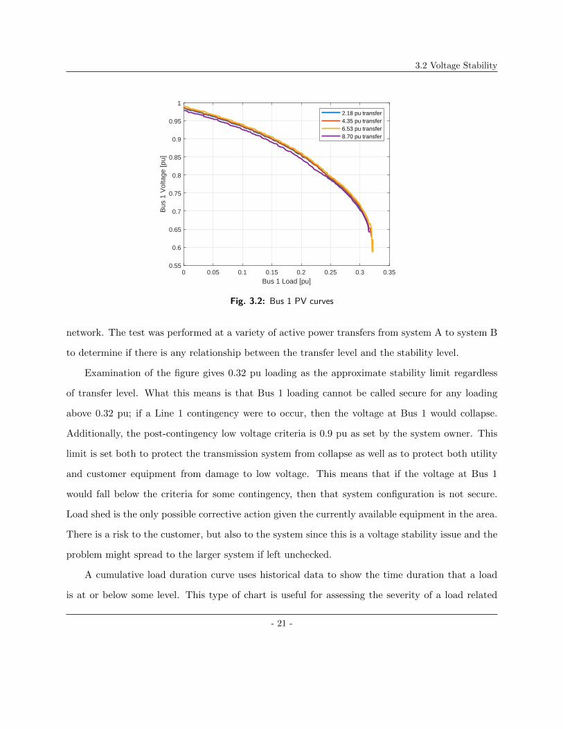
Figure 3.2 shows some partial PV curves where P is the load at Bus 1 and V is the voltage at
Bus 1 after Line 1 has been removed from service (i.e. serving Bus 1 load from system B). These
curves were empirically determined using a detailed system power flow model. Line 1 was removed
from service and the load at Bus 1 was increased incrementally until PSSE could not solve the
- 20 -
3.2 Voltage Stability
0 0.05 0.1 0.15 0.2 0.25 0.3 0.35
Bus 1 Load [pu]
0.55
0.6
0.65
0.7
0.75
0.8
0.85
0.9
0.95
1
Bus
1 V
olta
ge [p
u]
2.18 pu transfer4.35 pu transfer6.53 pu transfer8.70 pu transfer
Fig. 3.2: Bus 1 PV curves
network. The test was performed at a variety of active power transfers from system A to system B
to determine if there is any relationship between the transfer level and the stability level.
Examination of the figure gives 0.32 pu loading as the approximate stability limit regardless
of transfer level. What this means is that Bus 1 loading cannot be called secure for any loading
above 0.32 pu; if a Line 1 contingency were to occur, then the voltage at Bus 1 would collapse.
Additionally, the post-contingency low voltage criteria is 0.9 pu as set by the system owner. This
limit is set both to protect the transmission system from collapse as well as to protect both utility
and customer equipment from damage to low voltage. This means that if the voltage at Bus 1
would fall below the criteria for some contingency, then that system configuration is not secure.
Load shed is the only possible corrective action given the currently available equipment in the area.
There is a risk to the customer, but also to the system since this is a voltage stability issue and the
problem might spread to the larger system if left unchecked.
A cumulative load duration curve uses historical data to show the time duration that a load
is at or below some level. This type of chart is useful for assessing the severity of a load related
- 21 -

3.2 Voltage Stability
0 0.1 0.2 0.3 0.4 0.5 0.6
Bus 1 Load [pu]
0
10
20
30
40
50
60
70
80
90
100
Cum
ulat
ive
Dur
atio
n [%
of t
ime]
Load FrequencyStability Limit
Fig. 3.3: Bus 1 load duration curve
problem since the amount of time that the problem is present can be determined. Figure 3.3 shows
the load duration curve for Bus 1 using historical data from 2018. For example, the minimum
Bus 1 load approximately 0.13 pu during 2018. This is determined by looking at where the curve
first rises above the horizontal axis. Similarly, the bus load level never exceeded 0.52 pu since this
is where the curve reaches the top of the chart. The stability limit taken from Figure 3.2 is shown
as a red line on Figure 3.3.
Bus 1 was loaded at or below the stability limit of 0.32 pu for approximately 70% of 2018.
This means that Bus 1 presented a potential stability concern for 30% of 2018. Furthermore, the
post-contingency voltage criteria (0.9 pu voltage) is violated around 0.15 pu loading which means
that Bus 1 was not secure due to low voltage criteria for more than 90% of 2018. This issue was
addressed by the system owner through load transfers and using planned load shed.
Shedding load is obviously undesirable because this results in customers losing power. Load
transfers are also undesired because they typically require manpower to perform (which means they
- 22 -

3.3 Summary
are slow and operationally expensive) and while they mitigate the concern at Bus 1, it comes at
the cost of burdening other system buses (not shown in system schematic).
3.3 Summary
In this chapter, a transmission system with constraints is presented. Details of the voltage stability
constraint and its relationship to load level were explored.
- 23 -

4. Proposed Solutions
Chapter 4
Proposed Solutions
4.1 Reactive Power Injection
The voltage stability issue at Bus 1 may be sensitive to nearby reactive power injection. This can
easily be tested using the power flow model by injecting reactive power at Bus 1 and measuring the
voltage at some given operating point. If the relationship is strong then reactive power injection
is a viable solution to fix the voltage stability issue. There are many ways to implement reactive
power injection.
4.1.1 Capacitors
The simplest option to inject reactive power into the grid is by using capacitors. The capacitor
generates reactive power proportionally to the voltage squared and does not require any active power
(conductor losses aside). The squared relationship to voltage is problematic when using capacitors
to support voltage since when the voltage is low, the reactive power generating capability of the
capacitor is much lower. Conversely, when the capacitor is in service and the voltage is tending
upwards, it will generate more reactive power and thus exacerbate the voltage trend. Despite
- 24 -

4.1 Reactive Power Injection
Line 2Line 1
Bus 1
x N
Fig. 4.1: Schematic of switched capacitor banks at Bus 1 as modeled
this, capacitors can be an attractive solution to a utility when only basic controls are required
since this is the lowest cost solution to provide reactive power. Capacitor banks can either be
controlled manually or automatically however typically they have almost no ability to provide
transient voltage benefits. Fast switching capacitors are available which can switch quickly enough
to prevent transient drops in voltage but their benefit is limited to that. Transient controls related
to damping are not possible. In addition, capacitor banks must be switched in blocks which means
that reactive power can only be provided in discrete steps. Theoretically the steps can be made
very small, however in practice this does not work due to the increased cost of switches and controls
in comparison to the benefit gained with smaller steps.
• Power Flow Model Implementation
A detailed power flow based model was available for study. This model contains detailed steady
state models of the transmission systems in System A and System B as well as all of the surrounding
transmission systems and some of the more significant distribution systems. The model cannot be
disclosed due to the confidentiality agreements. A shunt capacitor was inserted at Bus 1 exactly as
shown in Figure 4.1. Note that the dotted line between Bus 1 and Line 1 represents an open branch.
This means that Bus 1 load is being fed radially by Line 2 which is the system configuration of
- 25 -

4.1 Reactive Power Injection
interest. The capacitor was sized with varying numbers of banks available; each bank was sized
to 0.1 pu. Note that this size is arbitrary and was simply selected at a reasonable and convenient
level consistent with other similar capacitors in the system.
The power flow model is not capable of simulating dynamic performance however in this case
that is not necessary. Instead, the control characteristic of the capacitor with respect to the voltage
can be determined by varying a model parameter by a small amount and then solving the model.
The capacitor banks were not modeled with any control system however in each step the capacitors
were controlled in a manner that would be consistent with how a human operator would control
the devices. In practice there would be some hysteretical effects however those are not of interest
to this study and were not considered.
A simple test procedure can be used to experimentally determine the effectiveness of a fixed
capacitor based solution. This procedure models how human system operators would control man-
ually switched capacitors:
1. Place a switchable capacitor with some number of blocks at Bus 1,
2. Increment the load at Bus 1 until one of the following:
(a) If the voltage at Bus 1 drops below 0.9 pu and a capacitor bank is available, then switch
in a capacitor bank and return to step 2
(b) Else if the model does not solve then stop
• Analysis
Figure 4.2 shows PV curves between load at Bus 1 and voltage at Bus 1 for a Line 1 contingency
which were generated using the test procedure. The number of available capacitor banks was varied
and is shown in the legend. The step changes in voltage that appear in the figure are the load levels
at which additional banks were required. The “0 cap banks” curve is the same curve as shown in
Figure 3.2 since this is the case where there are no capacitor banks available. Additional numbers
- 26 -

4.1 Reactive Power Injection
0 0.05 0.1 0.15 0.2 0.25 0.3 0.35 0.4 0.45 0.5
Bus 1 load [pu]
0.55
0.6
0.65
0.7
0.75
0.8
0.85
0.9
0.95
1
1.05
Bus
1 v
olta
ge [p
u]
0 cap banks1 cap banks2 cap banks3 cap banks
Fig. 4.2: Switched capacitor banks - PV curves
of available capacitor banks beyond 3 were simulated however it was found that the model would
stop solving before the 4th capacitor bank was required. Inspection of Figure 4.2 shows that adding
capacitor banks to Bus 1 would allow an increase in the stability limit up to approximately 0.45 pu
load. At this point the system becomes very unstable and the model is unable to solve even when
additional capacitor banks could be available.
By comparing the new stability limit against the load duration curve in Figure 3.3, it can be
seen that the increase in stability limit is insufficient to cover all expected load levels. The loading
at Bus 1 is below 0.45 pu approximately 95% of the time. This leaves 5% of the time where either
the system may be insecure, or load shedding may be required. It is possible that reducing the size
of individual capacitor blocks and having more blocks could extend the voltage stability beyond
0.45 pu; however this adds additional cost due to the extra switches and controls. Doing so would
move the system closer to a continuously controllable system.
- 27 -

4.1 Reactive Power Injection
4.1.2 Continuously Controllable Reactive Power Injection
There is more than one way to generate reactive power with continuous control. This section will
describe two possible devices which can both meet the requirement: Static VAr Compensator, and
Static Synchronous Compensator [14]. In a steady state power flow analysis, these two devices
appear to the system to be identical; therefore the analysis of one of them applies to both of them
and will appear at the end of this section. Note that the transient behavior of these devices is quite
different from each other and would require separate simulations for analysis.
• Static VAr Compensator
A Static VAr Compensator, or SVC, is a power electronics based device which can provide reactive
power support to the grid. A very simple SVC connected to Bus 1 is shown in Figure 4.3. It consists
of a capacitor and an inductor which are both individually switched with thyristors. In the design
shown in the figure, the capacitor provides reactive power and the inductor can absorb reactive
power which gives this device two modes of operation. In some cases the capacitor is not switched
via thyristor and instead is switched with a mechanical switch. In either case the inductor is required
in all modes of operation in order to provide continuous control when generating reactive power
since a switched capacitor is only discretely controllable. The advantage of switching the capacitor
with thyristors is enhanced speed of control of the capacitors. Mechanical switches could only react
to slowly varying system conditions. An SVC requires a power supply to perform switching and
thus consumes active power while operating. SVC switching is on the same order of magnitude
as the system frequency and thus generates significant low order harmonics. Harmonic filtering is
likely required (not shown in the figure), increasing both the cost and footprint of the device.
An SVC in steady state effectively switches the reactive elements in such a way that they
generate reactive power equivalent to a smaller static element. Thus the elements of an SVC
appear to the grid to be of varying size; however only smaller sizes are possible. For example, this
- 28 -

4.1 Reactive Power Injection
Line 2Line 1
Bus 1
Fig. 4.3: Schematic of an SVC at Bus 1
means that the SVC is not capable of generating more reactive power than the capacitor would have
been able to had it simply been a static capacitor. The maximum operating point of the SVC is the
same as the corresponding passive device (inductor or capacitor), had it been directly connected
to the grid. Since the SVC is just switching reactive devices, the squared voltage relationship
still remains. This is again problematic when voltage support is required since the reactive power
generating capability is reduced when it is needed most. However, an SVC provides an advantage
over a static capacitor when the voltage is high because it can switch its elements to provide less
reactive power.
The main benefit of an SVC over a simple capacitor is the ability to inject reactive power
across a continuous range (not just discrete values) and thus have better control over bus voltages.
The SVC allows for continuously variable output to meet the exact reactive power requirement. In
addition, SVCs can react quickly to transient conditions and can provide benefits such as damping
and transient voltage stability. The disadvantage compared to a simple capacitor is cost and
- 29 -

4.1 Reactive Power Injection
footprint. An SVC is much more expensive than fixed capacitors, it has a larger footprint (i.e.
occupies more physical space), and has a higher operating cost (both maintenance and flactive
power consumption). A utility may choose to incur the additional expense and build an SVC when
transient voltage support is required since a simple capacitor can not provide this.
• Static Synchronous Compensator
A Static synchronous Compensator, STATCOM, is also a power-electronics based device which
can provide reactive power support to the grid. It consists of a voltage source converter (VSC)
represented by the block with a diode and a DC capacitor. A simple schematic of a STATCOM
connected to Bus 1 is shown in Figure 4.4. The capacitor maintains a constant DC voltage which is
used by the VSC to generate an AC voltage in order to transmit reactive power. It functions very
similarly to an SVC in that it can provide reactive power to the grid in two modes of operation.
It can either generate or absorb reactive power; however the capacity of the STATCOM is directly
proportional to the terminal voltage. This is major advantage when compared to an SVC which has
a squared relationship to the voltage. This means that when reactive power generation is required,
the STATCOM’s capability is not reduced to the extent that an SVC’s capability would be.
An SVC is capable of generating or consuming only reactive power; the same is not true of
a STATCOM. A battery-based energy storage device typically uses an AC voltage source which
is converted to DC to charge the batteries. It is also capable of turning the DC back into AC to
discharge the batteries. If the device which is used to do this is a voltage source converter then
it is effectively a STATCOM with energy storage. The addition of energy storage is optional and
is not required for a STATCOM. However a device with energy storage would be capable of four
modes of operation since it could generate or consume both active and reactive power. For the
analysis performed in this section, only the reactive modes of operation will be considered. The
active modes of operation will be discussed in future sections.
- 30 -

4.1 Reactive Power Injection
Line 2Line 1
Bus 1
Fig. 4.4: Schematic of a STATCOM at Bus 1
A STATCOM should be switched at least at a switching frequency on the order of 1 kHz (at
least ten times the grid frequency). This reduces the filtering requirement by comparison to an
SVC. The footprint requirement of a STATCOM is comparable to an SVC however the reduced
filtering allows for a slightly smaller footprint for the STATCOM. A STATCOM also has comparable
requirements to an SVC for operating costs (maintenance and active power consumption).
• Analysis of SVC and STATCOM in Steady State
From a steady state perspective, both the SVC and the STATCOM inject reactive power into the
grid in the same way. This impact can be easily simulated using a detailed power flow model. The
same model was used as that which was used in section 4.1.1 to perform the analysis of the simple
capacitor solution. A shunt reactive device with continuous control and a voltage set point was
inserted at Bus 1 instead of a static shunt device with blocks. This is shown in Figure 4.5. Note that
the figure shows the label ”SVC” however the same variable shunt reactive model is representative
of a STATCOM in steady state. An SVC or STATCOM would require a control system with some
dynamic characteristic, however the dynamics of such a system cannot be modeled in a power flow
- 31 -

4.1 Reactive Power Injection
Line 2Line 1
Bus 1
SVC
Fig. 4.5: Schematic of the SVC as modeled
model. Therefore it is only possible to consider steady state performance of the control system.
For this study the control system is assumed to bring the voltage to 1 pu in steady state. A similar
test procedure can be used to determine the steady state control characteristic as in the simple
capacitor case:
1. Place an infinite variable capacitor at Bus 1 with voltage set-point at 1 pu
2. Increment the load at Bus 1 until the model no longer solves
Figures 4.6 and 4.7 were generated using this procedure and show the impact of an SVC at
Bus 1 for a Line 1 contingency. Each point on these plots was obtained by setting the load, solving
the power flow, and measuring the required reactive power injection. Putting all of the points
together forms the lines shown in each of the plots. Figure 4.6 shows a PV curve of voltage at
Bus 1 vs the load at Bus 1. Since the SVC is infinite, this PV curve is trivially just a straight line
with the voltage held at 1.0 pu for all load levels. The figure does indicate that an infinite SVC
could extend the voltage stability limit up to approximately 1.0 pu loading. This is more than
enough to cover the historical peak load of approximately 0.52 pu. No other information can be
obtained from the figure.
- 32 -

4.1 Reactive Power Injection
0 0.2 0.4 0.6 0.8 1 1.2
Bus 1 load [pu]
0
0.2
0.4
0.6
0.8
1
1.2
1.4
1.6
1.8
2
Bus
1 v
olta
ge [p
u]
Fig. 4.6: Infinite SVC PV curve
Figure 4.7 shows a PQ curve of the SVC output vs the load at Bus 1. This figure is much
more informative since it is the steady state control characteristic of an infinite SVC at Bus 1. It
demonstrates the VAr requirement for each load level. This information can be used to determine
the sizing requirement of an SVC. For example the required size for an SVC to ensure stability up
to the historical peak load is approximately 0.3 pu. This means that either an SVC or a STATCOM
of sufficient size is capable of resolving the voltage stability issue up to and beyond historical peak
loading.
- 33 -

4.1 Reactive Power Injection
0 0.2 0.4 0.6 0.8 1 1.2
Bus 1 load [pu]
-0.2
0
0.2
0.4
0.6
0.8
1
1.2
1.4
1.6
Bus
1 M
VA
r re
quire
men
t [pu
]
Fig. 4.7: Infinite SVC PQ curve
4.1.3 Transfer Capability Sensitivity to VAr Injection
Up to this point, voltage stability has been the main focus of the problem. From the results
demonstrated so far, it is clear that a simple capacitor based solution is insufficient to resolve the
voltage stability problem however a properly sized SVC or STATCOM based solution is sufficient.
The transfer capability issue must now be discussed.
Of the devices discussed so far, a STATCOM with energy storage will be the first device
considered for the transfer capability problem. This is because it has the most capability of any of
the devices since it has four modes of operation. The transfer capability problem requires a slightly
different model than for the voltage stability problem. In the voltage stability problem analysis,
a model with Line 1 out of service was used since this is when the problem manifests. However
with Line 1 out of service, Bus 1 becomes a radially fed load from system B and thus no transfer
is possible. Instead the system configuration of interest is when Line 1 is in service and Line 3 is
out of service. This system configuration will be used for the analysis. The same shunt reactive
- 34 -

4.1 Reactive Power Injection
0 0.05 0.1 0.15 0.2 0.25 0.3 0.35 0.4 0.45
Bus 1 load [pu]
0.68
0.7
0.72
0.74
0.76
0.78
0.8
0.82
Line
2 c
urre
nt [p
u]
Fig. 4.8: Line 2 flow vs Bus 1 load characteristic
device as for the STATCOM analysis is used again (see Figure 4.5). The difference for this analysis
is that the load at Bus 1 is modulated to model energy storage. At this stage, the energy capacity
of the device is not considered.
Considering a STATCOM with energy storage, there are two parameters at Bus 1 which can be
controlled in order to influence the flow on Line 2. Either reactive power injection or active power
injection are possible. Active power injection can be used to make the load at Bus 1 appear either
smaller or larger as required. Figure 4.8 shows the control characteristic of load changes at Bus 1
to the flow on Line 2. Each point on the line is obtained by setting the load at Bus 1 and solving
the power flow, then measuring the current flow on Line 2. The approximate sensitivity obtained
from the plot is -0.25. This is relatively small since it would take a variation in load of almost the
entire historical range just to influence the flow on the line by 0.1 pu. Given that the rating of the
line is 1.0 pu this is not a viable control parameter.
Reactive power injection can be used for voltage magnitude control. Figure 4.9 shows the
control characteristic of the voltage magnitude at Bus 1 to flow on Line 2. Each point on the
- 35 -

4.1 Reactive Power Injection
0.9 0.95 1 1.05 1.1 1.15
Bus 1 voltage [pu]
0.795
0.8
0.805
0.81
Line
2 c
urre
nt [p
u]
Fig. 4.9: Line 2 flow vs Bus 1 voltage characteristic
line is obtained by setting the reactive power injection at Bus 1 and solving the power flow, then
measuring both the current flow on Line 2 and the voltage at Bus 1. Note that the jagged parts
of the curve are caused by nearby voltage control devices such as transformer tap changers (not
shown in the system schematic). The approximate sensitivity obtained from the figure is -0.075.
This means that effective control of the flow on line is not possible even by varying the voltage
magnitude across the entire secure voltage range.
In both figures, the sensitivity of flow on the line to either voltage or load is very small.
Therefore, neither of these parameters can be used to solve the transfer capability problem. This
exhausts the control parameters of a STATCOM with energy storage and therefore such a device
is not sufficient to address the power transfer problem.
- 36 -

4.2 Unified Power Flow Controller
Fig. 4.10: Schematic of a basic UPFC
4.2 Unified Power Flow Controller
A Unified Power Flow Controller, or UPFC, is a power electronics based device which has two
functions. The first is to provide reactive power support to the grid in the same manner as a
STATCOM. In fact a UPFC contains a Statcom within it as one of its components. The additional
part of a UPFC that makes it different than a STATCOM is a second VSC which is connected to a
transformer which has one winding in series with a transmission line. Since a UPFC is essentially
two STATCOMs, it has approximately double the footprint and operating cost requirements [14].
A simple schematic of a UPFC is shown in Figure 4.10.
The additional series connection allows the UPFC to inject a series voltage onto the trans-
mission line. From the system perspective, this looks like a variable impedance in series with the
transmission line. By controlling the series voltage injected on the line, the UPFC can make the
transmission line appear to have a different impedance. This is useful when there are several paral-
lel lines and it is desired to control how power flow is shared among the parallel lines. For example,
the impedance of the line with the UPFC can be made to look larger than the other parallel lines
which would push power off of the controlled line and onto the other lines. Similarly, the apparent
impedance of the line could be made to look smaller which would cause more power to flow along
the line.
- 37 -

4.2 Unified Power Flow Controller
Line 1 Line 2
Bus 1
UPFC
Fig. 4.11: Schematic of the UPFC at Bus 1 as modeled
4.2.1 UPFC Steady State Analysis
Using the characteristics of a UPFC, a model suitable for a power flow solution can be constructed
using just 2 elements: a continuously variable impedance in series with a transmission line, and
a continuously variable shunt reactive device at a nearby bus. Figure 4.11 shows a schematic of
a UPFC model inserted into the system of interest in this way. The series impedance is inserted
in series with Line 2 and the shunt reactive element is located at Bus 1. Although the series
impedance is shown as an inductor, this does not fully represent the series part of a UPFC because
an inductor does not absorb or supply active power. In general it should be modeled as a variable
voltage source. Similarly, the shunt device is shown as a capacitor however again this does not
fully represent a UPFC. In general this should be modeled as a variable current source. In both
cases the active power characteristics of a UPFC can’t be represented with purely reactive devices.
A purely reactive UPFC model was used because a source-based model can’t be easily modeled in
PSSE and in this case a purely reactive model is sufficient to demonstrate that a UPFC has the
required control characteristics. This model was inserted into the detailed power flow model used
in previous sections. The parameters of the model were varied in order to obtain the steady state
control characteristic of the model.
This model was used in a system configuration set up such that Line 2 was overloaded in order
to demonstrate the ability to satisfactorily control the flow on the line and the voltage at Bus 1. The
- 38 -

4.2 Unified Power Flow Controller
0 0.1 0.2 0.3 0.4 0.5 0.6 0.7 0.8
Line 1 injected impedance [pu]
0.9
1
1.1
1.2
1.3
1.4
1.5
1.6
Line
2 c
urre
nt [p
u]
Fig. 4.12: UPFC series impedance vs Line 2 current
impedance was varied in small steps and the model was solved while monitoring the current flow
on Line 2. At the same time, the shunt device was used to control Bus 1 to 1.0 pu voltage. Each of
these solved power flows represents one point of data. Figure 4.12 shows a plot of the impedance
of the series element against the current on the line. This curve represents the steady state control
characteristic of current with respect to impedance for this system configuration. Figure 4.13 shows
a plot of the impedance of the series element against the reactive power injection required at Bus 1
in order to maintain the bus voltage at 1.0 pu. This curve can be thought of as a corollary control
characteristic for this system condition. The jagged parts of the curve are caused by nearby voltage
control devices reacting to the change in current on Line 2 and any associated voltage deviations
at their control buses. The voltage at Bus 1 is not shown in a figure since it is trivially held at
1.0 pu voltage identically to the curve shown in Figure 4.6.
The voltage stability problem is trivially solved since a UPFC has the same capability as a
STATCOM, and it was demonstrated in section 4.1.2 that a STATCOM is sufficient to resolve the
issue. Figure 4.12 demonstrates that it is feasible to solve the transfer capability problem using a
- 39 -
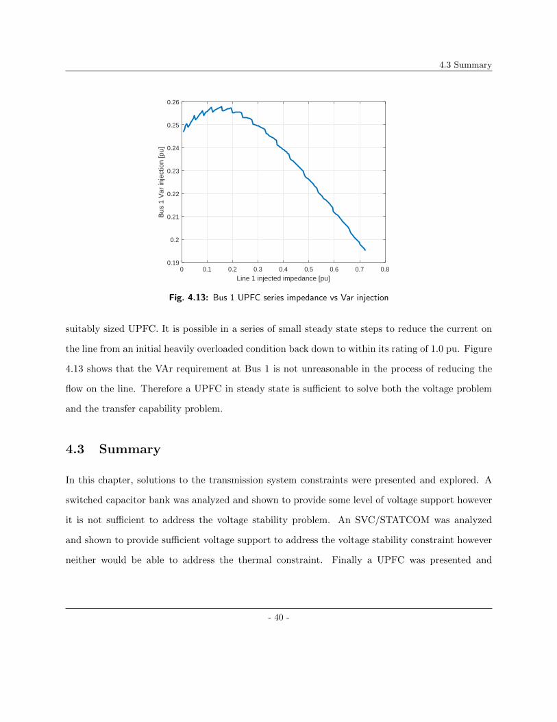
4.3 Summary
0 0.1 0.2 0.3 0.4 0.5 0.6 0.7 0.8
Line 1 injected impedance [pu]
0.19
0.2
0.21
0.22
0.23
0.24
0.25
0.26
Bus
1 V
ar in
ject
ion
[pu]
Fig. 4.13: Bus 1 UPFC series impedance vs Var injection
suitably sized UPFC. It is possible in a series of small steady state steps to reduce the current on
the line from an initial heavily overloaded condition back down to within its rating of 1.0 pu. Figure
4.13 shows that the VAr requirement at Bus 1 is not unreasonable in the process of reducing the
flow on the line. Therefore a UPFC in steady state is sufficient to solve both the voltage problem
and the transfer capability problem.
4.3 Summary
In this chapter, solutions to the transmission system constraints were presented and explored. A
switched capacitor bank was analyzed and shown to provide some level of voltage support however
it is not sufficient to address the voltage stability problem. An SVC/STATCOM was analyzed
and shown to provide sufficient voltage support to address the voltage stability constraint however
neither would be able to address the thermal constraint. Finally a UPFC was presented and
- 40 -

4.3 Summary
analyzed, and shown to sufficiently resolve both of the constraints. A UPFC is selected as the most
suitable solution and is the subject of study in subsequent chapters.
- 41 -

5. Dynamic Modeling
Chapter 5
Dynamic Modeling
5.1 Control System
5.1.1 UPFC Shunt Controls
All analysis until this point has been performed in a power flow program which requires only
minimally active controls (e.g. a voltage set point). A detailed analysis of the control action is
required before a dynamic model can be constructed. Let’s begin with a simple power transfer
across a reactor as shown in Figure 5.1. In this example the UPFC terminal would be on the
left side and the power grid would be on the right side. This is a useful analysis since the power
flow across a reactor provides insight into the characteristics of many devices, such as an ideal
transformer or a lossless transmission line. Note that a transmission line (lossless or otherwise) has
capacitance which may be significant however it is not necessary to model the capacitance for this
analysis. The shunt part of a UPFC is connected to the grid through a transformer therefore this
model is applicable. Consider the receiving end voltage with magnitude Vr as the reference voltage
with angle 0 and the sending end current with magnitude Is and phase angle θ with respect to the
- 42 -

5.1 Control System
Is∠θ Vr∠0jX
Fig. 5.1: A reactor with current flowing through it
receiving voltage. Convert the phasor from polar notation to rectangular notation with j as the
complex unit as follows
Vr 6 0 = Vrcos (0) + jVrsin (0) = Vr (5.1)
Is 6 θ = Iscos (θ) + jIssin (θ) (5.2)
Therefore the power which enters the grid at the receiving end is
P + jQ = Vr (Iscos (θ) + jIssin (θ))∗ (5.3)
From which is derived
P = VrIscos (θ) (5.4)
Q = −VrIssin (θ) (5.5)
Note that the power leaving the terminals of the UPFC must also include the power consumed
by the reactor and therefore is
Pt + jQt = Vr (Iscos (θ) + jIssin (θ))∗ + jI2sX (5.6)
- 43 -

5.1 Control System
However the extra power consumed by the reactor does not influence the behavior of the
receiving end and is therefore neglected. If the sending end current angle is set θ = 0◦, then
equations 5.4 and 5.5 simplify to
P = VrIs (5.7)
Q = 0 (5.8)
Observe that the reactive power transfer is zero. This means that if the sending end current is in
phase with the receiving end voltage then the active power transfer can be controlled independently
without any reactive power transfer. All that is needed to accomplish this is for the sending end
current to be in phase with the receiving end voltage and the magnitude can be varied to control
the power. Now set θ = 90◦, then equations 5.4 and 5.5 simplify to
P = 0 (5.9)
Q = −VrIs (5.10)
Note that in this case, the active power transfer is zero and the reactive power transfer is not.
All that is necessary to accomplish this is for the sending end current to be in quadrature with the
receiving end and then the magnitude can be varied to control the power.
With these two observations in mind, a sending end current will be constructed with two
components, one in phase and one in quadrature to the receiving end. The in-phase component
is designated Id and the quadrature component is designated Iq. These two components can
independently control both the active and reactive powers at the same time. A control system
- 44 -

5.1 Control System
mq cos(ωt + 𝛿)
md sin(ωt + 𝛿)
+ -
Vdc_ref
Vdc_meas
PLLVr_meas
md
𝛿
+-Vr_ref
Is+
mq
PID
PID
Id
Iq
LPfilter
LPfilter
Fig. 5.2: UPFC shunt control system
for the shunt part of a UPFC can be derived from this since the device is capable of producing
arbitrary voltage waveforms. The shunt device will be used for two purposes: to control the AC
bus voltage, and to control the DC bus voltage. The reactive power transfer from the shunt device
directly influences the bus voltage, and the active power transfer directly influences the DC bus
voltage. Therefore it is convenient to select these two quantities as the control variables rather
than directly controlling power transfer.
Note that the assumption that the receiving end voltage is constant may not be true. If
the receiving end voltage varies with power transfer then the active and reactive controls will
be coupled. Uncoupling the controls requires knowing how the receiving voltage varies with power
transfer which in turn requires knowing the network impedance behind the voltage. This is difficult
knowledge to obtain since measuring the network impedance in general is not easy and it may vary
with changing network conditions. Therefore the control system will assume constant receiving
voltage in favour of simplicity at the cost of some potential coupling between active and reactive
components.
- 45 -

5.1 Control System
Figure 5.2 shows the control system derived from the analysis. The signals in the figure are
as follows: Vdc ref is the DC voltage reference, Vdc meas is the measured DC voltage, Vr ref is the
grid bus voltage reference, Vr meas is the measured grid bus voltage, Is is the sending end current
signal. Both measured signals will go through low pass filters to remove high frequency noise
before entering the PID controllers. Two PID controllers are used to control the magnitudes of
the components based on error signals from the measured quantities. The mdsin(ωt + δ) block
will produce a sinusoid that is in phase with the measured AC bus voltage and therefore controls
active power as shown in equations 5.7 and 5.8. The mqcos(ωt + δ) block will produce a sinusoid
that is in quadrature with the measured AC bus voltage and therefore controls reactive power as
shown in equations 5.9 and 5.10. A Phase Locked Loop (PLL) is used to track the phase angle of
the receiving end voltage which then feeds into the two sinusoidal components. The sending end
current signal is constructed by summation. This signal will be passed to the UPFC shunt device
which will translate it from a signal into a physical current. The mechanism by which this is done
will be discussed in future sections.
5.1.2 UPFC Series Controls
A schematic of the series part of a UPFC is shown in Figure 5.3. The UPFC is connected to the
sending end of a transmission line through a transformer connected in series with the transmission
line. The transmission line is represented by the inductor on the right. The output current of the
UPFC will be directly proportional to the line current according to the transformer winding ratio.
Therefore if the control system directly controls the output current of the UPFC, then the power
flow down the line can be directly controlled. From this perspective the series control system and
equivalent circuit becomes identical to that considered in the shunt case. All of the same analysis
holds true and the control system is directly obtained.
- 46 -

5.1 Control System
Vs∠0 jXIs∠θ
Is∠θ
UPFC
Fig. 5.3: Series components of a UPFC with current flow
Figure 5.4 shows a schematic of the series element control system where Pmeas is the measured
active power flow down the line, Qmeas is the measure reactive power flow down the line, and
Vs is the sending end voltage (from the perspective of the transmission line). Error signals are
filtered before entering separated PID controllers. The PID controllers generate the component
magnitudes which are then constructed into a sinusoidal signal which is passed on to the valve
group. The control system architecture is identical to the shunt control system.
- 47 -

5.1 Control System
mq cos(ωt + 𝛿)
md sin(ωt + 𝛿)
+ -Pref
Pmeas
PLLVs_meas
md
𝛿
+ -Qref
Is+
mq
PID
PID
Id
Iq
Qmeas
LPfilter
LPfilter
Fig. 5.4: UPFC series control system
5.1.3 Hysteresis Current Control
Both shunt and series control systems directly generate the desired converter current output signal,
therefore a switching scheme which directly generates a physical current is required. Hysteresis
current control is the switching method selected.
For a PWM based voltage source converter, the control system directly generates the desired
voltage waveform signal and the switching is performed to convert it to a physical voltage. If the
switching frequency is very high compared to the signal, then the signal is converted approximately
one-to-one to the physical voltage (high order harmonics aside). In this paradigm, the switching
frequency can be specified as desired. Physical current appears as a secondary dynamic as a result
of whatever voltage waveform is generated. However it is possible instead to measure and directly
control the current.
- 48 -

5.1 Control System
+Vdc
L
-Vdc
Vdc(t) Vgrid(t)
iL(t)
Fig. 5.5: Single phase valve
Let’s consider Figure 5.5 which shows a single phase of a two-level valve group. The phase
current of this VSC obeys equation 5.11 where iL(t) is the phase current, Vdc(t) is the converter
output voltage waveform, Vgrid(t) is the AC grid voltage, and L is the phase reactor inductance.
d
dtiL(t) =
Vdc(t) − Vgrid(t)
L(5.11)
If the rate of change of current is very fast compared to Vgrid(t) then Vgrid(t) can be assumed
constant. This means that the current will simply increase or decrease linearly depending on
which level the VSC is outputting. The phase current will oscillate between linearly increasing and
linearly decreasing as the VSC switches between its two states. If the desired current signal also
varies slowly compared to the rate of change of current as determined by equation 5.11 then there
is the basis for a control system to directly generate a current waveform.
Let’s define Isig(t) to be the desired output current, and h to be the maximum deviation from
the desired current. Current directionality is with respect to exiting the converter. The control
method will be as follows. When the VSC is outputting its high voltage level then the current will
be increasing. When the current reaches Isig(t) + h then the VSC should switch to the low voltage
- 49 -

5.1 Control System
+Vdc
-Vdc
Isig + h
Isig - h
Fig. 5.6: Hysteresis Current Control
- 50 -

5.1 Control System
level. The current will decrease. When the current reaches Isig(t) − h then the VSC should switch
back to the high level. Figure 5.6 illustrates this control scheme. The vertical dotted lines in the
figure show the positive edge of the voltage waveform.
This is called hysteresis current control because the current waveform level oscillates within a
bound of the desired current signal. The current signal is directly generated and the voltage can
be thought of as a secondary dynamic of the current waveform. The disadvantage of this control
scheme is apparent in the figure. The spacing between vertical lines is the switching period and it is
not constant over one cycle; the switching period varies with the magnitude of the output current.
This makes AC filtering difficult compared to a voltage output control scheme. In a voltage output
scheme the switching frequency can be set constant and therefore AC filtering can be tuned to
match. With a varying switching frequency, the AC harmonics to filter out will also vary and
therefore passive tuned filters can’t be used.
Some basic characteristics of the frequency variation can be analyzed [15]. Assume switching is
fast enough that Vgrid(t) and Isig(t) are both approximately constant. The time tup of the current
increasing state is
tup =2hL
+Vdc − Vgrid(t)(5.12)
similarly, the time tdown spent in the current decreasing state will be
tdown =−2hL
−Vdc − Vgrid(t)(5.13)
the total switching period T is
T = tup + tdown =2hL
+Vdc − Vgrid(t)− 2hL
−Vdc − Vgrid(t)(5.14)
therefore switching frequency f is
- 51 -

5.2 Model Schematic
f =1
T=V 2dc − V 2
grid(t)
4VdchL(5.15)
The maximum switching frequency will occur when Vgrid(t) = 0 which gives
fmax =Vdc4hL
(5.16)
5.2 Model Schematic
Unlike in the steady state analysis, there was no model available to use for the dynamic analysis.
Therefore a model was developed in PSCAD and is shown in Figure 5.7. The solid lines represent
electrical components and the dotted lines and boxes represent control signals or measurements.
The voltage source on the left side of the figure is the Thevenin equivalent source for System A
and the voltage source on the right side of the figure is the Thevenin equivalent source for System
B. The angle of the System B source is arbitrary but was selected so that the initial flow on Line
2 was within its operating limits. The load on Bus 1 was set to a typical daily peak load.
The control system for the shunt part of the UPFC takes its measurements from the locations
shown in the figure. The voltage magnitude and angle from Bus 1, and the voltage magnitude of
the DC bus capacitor feed into the controller. The control system constructs the desired current
waveform and sends the control signals to the valve group.
The control system for the series part of the UPFC takes its measurements as shown in the
figure. The voltage angle from the sending end of Line 2, and the active and reactive power at the
sending end feed into the control system. The control system constructs the desired waveform and
feeds the control signals into the valve group.
Line 1 and Line 2 are modeled using the frequency dependent, conductor geometry based
models which are available in PSCAD. The geometrical parameters were obtained from the system
- 52 -

5.2 Model Schematic
ZaZb
Line 1 Line 2
Va∠0Vb∠θ
Bus 1
AC filters AC filters
ControlSystem
V, Ang V
ControlSystem
Ang,P, Q
Fig. 5.7: Full UPFC Model
- 53 -

5.3 Model Parameters
3
Fig. 5.8: Valve Group
owners and used in the model. Each of the shunt and series valve groups are made up of a two-level
VSC, each of which have AC filtering to remove some of the harmonics from the injected voltages.
The valve groups share a DC bus capacitor. Figure 5.8 shows a schematic of the valve group and
its AC filter. The AC filter is a simple second order low pass filter.
5.3 Model Parameters
The following sections detail the model parameters of the various components and control blocks.
• Station Load
The load on Bus 1 is a constant current load set to 0.482 pu active power and 0.104 pu reactive
power at 1.0 pu voltage.
• Transformers
The transformer parameters are shown in Table 5.1. The same transformer is used for both shunt
and series components.
- 54 -

5.3 Model Parameters
Table 5.1: Transformer parameters
MVA rating 0.65 pu
Winding ratio 10
Winding 1 Type wye
Winding 2 Type wye
Leakage reactance 0.06 pu
Copper losses 0.003 pu
Saturation None
Table 5.2: AC filter parameters
L 6.78 mH
C 115 µF
fo 300 Hz
• AC Filtering
The AC filtering for both the series and shunt elements are simple low pass LC filters. The
capacitor was selected to provide 0.1 pu MVAr at nominal voltage. The inductor was selected to
get the desired cutoff frequency of 300Hz. The parameters are shown in Table 5.2.
• DC Capacitor
The DC capacitor will provide the DC voltage which will be switched to produce an AC waveform
for interfacing with the grid. Nominal DC voltage will set at 123% of the nominal peak AC voltage.
This will provide ample room for variation in the AC output waveform.
The size of the capacitor will affect the size of the voltage ripple as well as converter dynamic
performance. The following equation relates the capacitor size C to its associate time constant τ
[16]
τ =energy stored
nominal power rating=CV 2
dc
2Pn(5.17)
- 55 -

5.3 Model Parameters
For this converter, the time constant has been selected as 2ms which produces capacitor size
of 375µF
• Current Hysteresis
The maximum switching frequency is selected to be 2000Hz. Equation 5.16 then provides the
maximum current error h to be 0.2pu.
• Control Signal Filtering
All error signals pass through a 4th order Butterworth low pass filter with cut off frequency of
500Hz.
5.3.1 PID Controllers
The integral components of every control system are internally limited to nominal peak current in
order to prevent windup. Additionally the sum of each PID group is hard limited to nominal peak
current to prevent the UPFC from attempting to produce current over nominal.
The shunt PID controllers have two sets of parameters. One set for strong-network conditions
(i.e. system intact) and a second set for weak-network conditions (i.e. post Line 1 contingency).
The controller parameters depend strongly on the coupling between the network and the UPFC.
When the network conditions change, the previous control parameters may no longer be suitable
for the new network condition. There are line protection relays at the station which detect fault
conditions and locations. These relays send signals to open the correct breakers to clear the fault.
The UPFC can co-opt the breaker open signal as a trigger for the controller to switch to the second
set of parameters. This signal will tell the controller to change its block gains and also to reset
the states in each integral block. Resetting the integral states is necessary because the faulted
network condition is likely to pin the internal integral state to one of its bounds which is a poor
- 56 -

5.3 Model Parameters
Table 5.3: Controller gains
PID component Strong network Weak network
shunt Id kp 1.72E-1 8.25E-2
shunt Id ki 2.51E+0 7.25E-1
shunt Id kd 0.00E+0 2.84E-5
shunt Iq kp 5.44E+1 7.44e+0
shunt Iq ki 3.60E+3 6.89E+1
shunt Iq kd 0.00E+0 9.41E-2
series Id kp 2.80E-4 N/A
series Id ki 1.26E+0 N/A
series Id kd 0.00E+0 N/A
series Iq kp 1.1E-3 N/A
series Iq ki 8.02E-1 N/A
series Iq kd 0.00E+0 N/A
initial condition for the UPFC to transition to post-fault operation. A typical time delay from fault
inception to fault clearing is five cycles (0.083 s).
Note that the loss of Line 1 will cause the station be radially fed from Line 2 which means that
the series element of the UPFC can no longer operate. Therefore the same trigger (fault clearing
signal to the breaker) will also cause the series element to block and bypass. In general, a different
parameter set could be determined for every relevant network condition. However in this case the
focus is the Line 1 contingency. The Line 2 contingency is not studied but may require a similar
study to determine suitable controller parameters for post fault network conditions.
Table 5.3 shows the gains for each block in every controller. The controller gains were de-
termined using simplex multi-variate optimization. This applies to both the strong-network and
weak-network parameter sets. The optimization was performed such that the sum of the control
error signal and DC voltage deviation were minimized. This approach provides a balance between
a fast control response and low DC voltage disturbance. DC voltage disturbance was selected as an
error signal source because DC voltage variation is detrimental to the UPFC performance. Note
that gains are displayed using shortened scientific notation.
- 57 -

5.4 Summary
5.4 Summary
In this chapter, a UPFC is designed in detail. The electrical components are selected. The control
system for the UPFC is built from a mathematical basis. The controller scheme is selected, designed,
and tuned using an optimization procedure.
- 58 -

6. Model Performance
Chapter 6
Model Performance
This chapter will present and discuss various performance aspects of the model developed in the
previous chapter.
6.1 Control system step responses
The first performance characteristic of the model which will be discussed is the step response to
the control parameters. Each of the following three parameters will be stepped: AC voltage, active
power, and reactive power. Note that the DC voltage control system will never receive any reference
changes since it is always controlled to 1 pu. Therefore, a step response for DC reference voltage
was not performed.
An acceptable step response must be obtained for each control parameter. This means that in
addition to a stable response, some criteria must be met. For controller step responses: controlled
parameter overshoot must not exceed 20% of the step size, AC bus voltage coupling must not exceed
0.01 pu, DC bus voltages must remain within the range 0.7 pu to 1.3 pu at all times, and power
coupling on Line 2 must not exceed 0.05 pu. Responses must settle within 0.167 s. The criteria
for system fault responses is different. During the fault, there is no criteria. Beginning with the
- 59 -

6.1 Control system step responses
first swing after the fault clears, both AC and DC voltages must remain within the range 0.7 pu
to 1.3 pu, and return to within the range 0.9 pu to 1.1 pu after the transient settles.
6.1.1 Voltage Reference Step Response
Figure 6.1 shows the step response to a 0.05 pu change in the AC voltage reference. Both a positive
step and a negative step are shown. The AC voltage response (top plot) shows a settling time of
approximately 0.1 s which is 6 cycles. There is some coupling to the DC voltage (middle plot)
which experiences an initial deviation of 0.08 pu followed by controller overshoot of approximately
0.025 pu. This is expected since the decoupling assumptions made in the design of the control
system are not perfectly accurate. The active power and reactive power response (bottom plot)
show almost no disturbance at all. Overall, these responses are well within the criteria.
- 60 -

6.1 Control system step responses
0 0.1 0.2 0.3 0.4 0.5 0.6 0.7 0.8 0.9 1
Time [s]
0.98
1
1.02
1.04
1.06
RM
S V
olta
ge [p
u]
VV
ref
0 0.1 0.2 0.3 0.4 0.5 0.6 0.7 0.8 0.9 1
Time [s]
0.9
0.95
1
1.05
1.1
DC
vol
tage
[pu]
VV
ref
0 0.1 0.2 0.3 0.4 0.5 0.6 0.7 0.8 0.9 1
Time [s]
0
0.1
0.2
0.3
0.4
0.5
Pow
er L
ine
1 [p
u]
PP
ref
ref
Fig. 6.1: Voltage reference step response
- 61 -

6.1 Control system step responses
6.1.2 Active Power Reference Step Response
Figure 6.2 shows the step response to a 0.1 pu change in the active power reference. Both a
positive step and a negative step are shown. The active power response (bottom plot) settling time
is approximately 0.15 s with a small overshoot of approximately 0.01 pu. The longer response is
intentional to minimize voltage disturbance caused by the change in power flow. The AC voltage
response (top plot) shows some coupling with a disturbance of approximately 0.003 pu. This is
well within the criteria. There is some coupling to the DC voltage (middle plot) which experiences
a deviation of approximately 0.015 pu. The reactive power response (bottom plot) shows coupling
of approximately 0.015 pu. There was no attempt to decouple the shunt elements (AC and DC
voltage control) from the series elements (active and reactive power control) therefore the coupling
is expected. The small amount of coupling between the active and reactive responses is due to the
assumptions made in the design stage. Namely, the transmission line was assumed to be lossless and
the source impedance behind the transmission line was not considered. However, these responses
are all within the criteria.
- 62 -

6.1 Control system step responses
0 0.1 0.2 0.3 0.4 0.5 0.6 0.7 0.8 0.9 1
Time [s]
0.98
1
1.02
1.04
1.06
RM
S V
olta
ge [p
u]
VV
ref
0 0.1 0.2 0.3 0.4 0.5 0.6 0.7 0.8 0.9 1
Time [s]
0.9
0.95
1
1.05
1.1
DC
vol
tage
[pu]
VV
ref
0 0.1 0.2 0.3 0.4 0.5 0.6 0.7 0.8 0.9 1
Time [s]
0
0.1
0.2
0.3
0.4
0.5
Pow
er L
ine
1 [p
u]
PP
ref
ref
Fig. 6.2: Active power reference step response
- 63 -

6.1 Control system step responses
6.1.3 Reactive Power Reference Step Response
Figure 6.3 shows the step response to a 0.1 pu change in the active power reference. Both a positive
step and a negative step are shown. The reactive power response (bottom plot) settling time is
approximately 0.15 s with a small overshoot of approximately 0.012 pu. Again, the longer response
is intentional to minimized voltage disturbance caused by the change in power flow. The AC voltage
response (top plot) shows some coupling with a disturbance of approximately 0.005 pu. This is
within the criteria. There is some coupling to the DC voltage (middle plot) which experiences
a deviation of approximately 0.025 pu. The active power response (bottom plot) shows coupling
of approximately 0.017 pu. There was no attempt to decouple the shunt elements (AC and DC
voltage control) from the series elements (active and reactive power control) therefore the coupling
is expected. The small amount of coupling between the active and reactive responses is due to the
assumptions made in the design stage. Namely, the transmission line was assumed to be lossless
and the source impedance behind the transmission line was not considered.
- 64 -

6.1 Control system step responses
0 0.1 0.2 0.3 0.4 0.5 0.6 0.7 0.8 0.9 1
Time [s]
0.98
1
1.02
1.04
1.06
RM
S V
olta
ge [p
u]
VV
ref
0 0.1 0.2 0.3 0.4 0.5 0.6 0.7 0.8 0.9 1
Time [s]
0.9
0.95
1
1.05
1.1
DC
vol
tage
[pu]
VV
ref
0 0.1 0.2 0.3 0.4 0.5 0.6 0.7 0.8 0.9 1
Time [s]
0
0.1
0.2
0.3
0.4
0.5
Pow
er L
ine
1 [p
u]
PP
ref
ref
Fig. 6.3: Reactive power reference step response
- 65 -

6.2 UPFC Fault Response
6.2 UPFC Fault Response
Figure 6.4 shows the baseline system response to a three-phase, close-in, bolted fault on Line 1
without the UPFC in service. The fault duration is five cycles. The bus voltage post fault is
0.82 pu. Therefore Line 2 cannot support the load at the station when the Line 1 breaker opens.
The bottom plot shows the power flow on Line 2. The power references are included on the plot
despite the UPFC being out of service.
Figure 6.5 shows the UPFC and system responses to the same fault. During the fault, the
AC bus voltage drops but recovers shortly after clearing with an overshoot of 0.05 pu. The DC
bus voltage drops during the fault but recovers with an overshoot of 0.07 pu. The bottom plot
shows the power flow on Line 2 which are controlled by the series element before the fault. The
blocking of the series element post-fault operates correctly, allowing the power to flow freely. The
fault response of the system meets the criteria.
6.3 Summary
In this chapter, all of the step responses are shown to be stable, and meet all criteria. The system
is shown to meet the fault response criteria.
- 66 -

6.3 Summary
0 0.1 0.2 0.3 0.4 0.5 0.6 0.7 0.8 0.9 1
Time [s]
0
0.2
0.4
0.6
0.8
1
1.2
RM
S V
olta
ge [p
u]
VV
ref
0 0.1 0.2 0.3 0.4 0.5 0.6 0.7 0.8 0.9 1
Time [s]
-0.6
-0.4
-0.2
0
0.2
0.4
0.6
Pow
er L
ine
1 [p
u]
PP
ref
ref
Fig. 6.4: Line 1 contingency without UPFC
- 67 -

6.3 Summary
0 0.1 0.2 0.3 0.4 0.5 0.6 0.7 0.8 0.9 1
Time [s]
0
0.2
0.4
0.6
0.8
1
1.2
RM
S V
olta
ge [p
u]
VV
ref
0 0.1 0.2 0.3 0.4 0.5 0.6 0.7 0.8 0.9 1
Time [s]
0
0.2
0.4
0.6
0.8
1
1.2
DC
vol
tage
[pu]
VV
ref
0 0.1 0.2 0.3 0.4 0.5 0.6 0.7 0.8 0.9 1
Time [s]
-0.6
-0.4
-0.2
0
0.2
Pow
er L
ine
1 [p
u]
PP
ref
ref
Fig. 6.5: Line 1 contingency with UPFC
- 68 -

7. Grid Storage
Chapter 7
Grid Storage
This chapter will explore the implications of combining grid storage with the UPFC from the
previous chapters.
7.1 Adding a Battery
There are two main components to a grid storage battery: the battery, and a DC-AC interface.
Additionally a buck-boost interface may be required for high voltage applications. The purpose of
the battery is self evident: to store and release the energy. Since batteries can only provide DC
voltage, the DC-AC interface must be able to translate the DC into AC for discharge operation
and also AC into DC for charging operation. In a low voltage application the battery voltage may
be high enough for the DC-AC interface to directly interface the battery with the AC system.
However, in a high voltage application, such as a grid storage battery, the battery voltage is not
likely to be large enough for direct interfacing. In cases such as these a buck-boost interface is
required. This interface can either be on the AC side in the form of a transformer or on the DC
side in the form of a DC-DC converter.
- 69 -

7.2 Battery Interface Topology
The UPFC that was presented in the previous chapter already contains a DC bus and a DC-
AC interface, therefore adding a battery to the system only requires interfacing the battery to
UPFC’s already existing DC bus. A buck-boost DC-DC converter fulfills the requirements. Figure
7.1 shows the UPFC system schematic with battery included. The battery controller uses the DC
link measurement and the battery voltage measurement as control inputs. It outputs switching
signals to the power electronics in the buck-boost converter, and a charge request signal to the
shunt controller.
Adding a battery to the system increases the cost of the system however it provides benefits to
the utility in the form of energy storage which may be used for things such as frequency control or
peak shaving. Further, active power injection may reduce the need to build additional generation
or transmission. The battery can store excess generation during periods of low loading and then
release it during periods of high loading. This allows for increased utilization of existing generation
while avoiding potential transmission constraints.
These benefits may be worth the additional costs on their own however the extra costs could be
offset by controller design. The series component of the UPFC must absorb or reject active power
in order to accomplish control of the flow on the transmission line. Typically the shunt system
will compensate for active power which is absorbed or released by the series system. However if
the battery instead provides the compensation then the shunt electrical components (such as AC
transformer) can be sized down to save on costs since they are no longer required to handle as much
power. The shunt controller instead acts as a low power battery charger without any series active
power delta compensation.
7.2 Battery Interface Topology
A simple 2-switch buck-boost converter will be used as the DC-DC interface for the battery. The
topology is shown in Figure 7.2. This converter has two switching states: S1 closed with S2 open
- 70 -

7.2 Battery Interface Topology
ZaZb
Line 1 Line 2
Va∠0Vb∠θ
Bus 1
AC filters AC filters
ControlSystem
V, Ang V
ControlSystem
Ang,P, Q
ControlSystem
V
Charge Request
Fig. 7.1: UPFC with battery
- 71 -

7.3 Model Parameters
+
L
-
Vbat(t)C
S1
S2
+
-
VUPFC-DC(t)
Ibat(t)
Fig. 7.2: Battery interface topology
which causes battery current Ibat(t) to decrease, and S1 open with S2 closed which causes battery
current to increase. The inductor L is required to smooth the battery current and the capacitor C
smooths the battery voltage.
7.3 Model Parameters
The converter uses an inductor size of 100 mH and capacitor size of 1 µF. The battery model is
a Shepherd model. A graphical depiction of the model is shown in Figure 7.3. The variables in
the figure are as follows. E(t) is the no load voltage, E0 is the battery constant voltage, K is
the polarization voltage, Q is the battery capacity, I(t) is the battery charge, A is the exponential
voltage amplitude, and B is the exponential zone time constant inverse [17]. Table 7.1 shows
the parameter values used in the model. Note that the parameters as shown in the table do not
correspond one-to-one with the variables in the equations shown in Figure 7.3 and they must be
transformed before use in the equations. The parameters are expressed in this way because this is
how they are entered in the PSCAD model.
- 72 -

7.3 Model Parameters
E(t)
+
-
Rbat
ibat(t)
(t)
E(t)
Vbat(t)
+
-Fig. 7.3: Shepherd model [17]
Table 7.1: Shepherd model parameters
Nominal voltage 25 % of UPFC DC nominal voltage
Rated capacity 0.217 pu
Loss of capacity at nominal current in an hour 100 %
Nominal capacity 0.95 pu
Resistive drop 0.0001 pu
Voltage at exponential point 1.03 pu
Capacity at exponential point 0.4 pu
Fully charged voltage 1.15 pu
- 73 -

7.4 Battery Control System
7.4 Battery Control System
7.4.1 Topology
The battery control system consists of a PID controller which generates the battery current refer-
ence. The reference current and the measured battery current feed into a hysteresis current control
signal generator which generates the switching signals for S1 and S2. This is shown in Figure 7.4.
In the previous iteration of the UPFC the shunt system was responsible for maintaining the DC
bus voltage. If the battery controller is added and also set to control the DC bus then these two
systems will fight for control of the bus. This is not desirable. To address this issue, the shunt
control system will be made to have a slow response to DC bus voltage deviations. Instead it will
be the responsibility of the battery control system to respond quickly to the DC bus voltage.
In many cases, a buck-boost DC-DC converter is used to control the output voltage of the
converter (in this case the output voltage is the effective battery voltage as seen by the DC bus
through the converter) however in this case current control is more appropriate. DC bus voltage
does not respond directly to the effective battery voltage but instead responds to the actual battery
current. Therefore current control will be able to respond more directly to bus voltage deviations.
A hysteresis current controller is used in order to simplify the controller topology at the cost of
variable switching frequency. Despite this, the target switching frequency is 2 kHz as in the other
UPFC components. A peak to peak current ripple of 0.03 pu accomplishes this.
Since the battery maintains the DC bus voltage, the shunt control system will handle the long
term charging of the battery. The modified shunt controller is shown in Figure 7.5; note that the
reactive power control is unchanged. Battery charging is accomplished by adding a droop feedback
with gain of 0.33 pu to the active power loop of the shunt control system and setting the shunt DC
bus voltage reference above nominal when the battery requests charging.
- 74 -

7.4 Battery Control System
+ -Vref
PID
Vmeas
LPfilter
S1(t)
S2(t)
HCC
Ibat(t)
Iref(t)
Fig. 7.4: Battery control system
Since the shunt system is now slow, it will slowly ramp up its active power intake until the
droop feedback causes the effective voltage reference to return to nominal. Meanwhile, the battery
will maintain the DC voltage at nominal and will absorb the excess power. When the battery has
reached its desired state of charge, it rescinds its request for charge which causes the shunt control
system voltage reference to return to nominal. The shunt control system will slowly ramp down the
active power consumption again until the effective voltage reference is nominal. When the battery’s
state of charge reduces sufficiently it will again request charge and the process will repeat.
7.4.2 Controller Gain
Battery and shunt system controller parameters were tuned using the same simplex optimization
procedure as before. However the battery control system was tuned by itself first with the new
shunt controller temporarily disabled. Then the shunt controller was enabled and re-tuned with
the new battery controller parameters in place. Tuning controllers in this order makes the battery
controller DC bus voltage response have priority while also making the shunt controller as fast as
possible without conflicting with the battery controller.
Unlike the shunt controller, the battery control response is not coupled to the network strength
in the same way that the shunt controller is. Therefore segmenting the controller parameters for
different network configurations is not necessary and the same controller gains can be used for
- 75 -

7.4 Battery Control System
+-+ -
mq cos(ωt + 𝛿)
md sin(ωt + 𝛿)
Vdc_ref
Vdc_meas
PLLVr_meas
md
𝛿
+-Vr_ref
Is+
mq
PID
PID
Id
Iq
LPfilter
LPfilter
kdroopChargeRequest
Fig. 7.5: Shunt controller with droop
both strong-network and weak-network conditions. However the shunt controller weak-network
parameters for active power were re-tuned due to the presence of the battery. Similar to before,
the UPFC will take advantage of the existing line protection to sense and signal the change of
network configuration. The UPFC shunt controllers will reset their integral states and switch to
weak-network gains. Although the battery will not switch its gains, it also must reset its integral
state. This is due to pinning of the controller during the fault which creates a poor initial condition
for post-fault-clearing operation.
- 76 -

7.5 Step Response with Battery
Table 7.2: Controller gains with battery
PID component Strong network Weak network
shunt Id kp 1.66E-2 1.22E-1
shunt Id ki 4.23E+0 1.11E-1
shunt Id kd 0.00E+0 1.34E-4
shunt Iq kp 5.44E+1 7.44e+0
shunt Iq ki 3.60E+3 6.89E+1
shunt Iq kd 0.00E+0 9.41E-2
series Id kp 2.80E-4 N/A
series Id ki 1.26E+0 N/A
series Id kd 0.00E+0 N/A
series Iq kp 1.1E-3 N/A
series Iq ki 8.02E-1 N/A
series Iq kd 0.00E+0 N/A
battery kp 7.11E-2 N/A
battery ki 1.29E+0 N/A
battery kd 5.33E-5 N/A
7.5 Step Response with Battery
All of the step response tests were redone and are shown in Figures 7.6, 7.7, and 7.8. The criteria
used to evaluate the system is the same as that used in the previous chapter. Comparison to the
previous step responses shows very similar results. When the battery is present, the DC voltage
response is slightly faster with slightly more overshoot. All of the step responses meet the criteria.
- 77 -

7.5 Step Response with Battery
0 0.1 0.2 0.3 0.4 0.5 0.6 0.7 0.8 0.9 1
Time [s]
0.98
1
1.02
1.04
1.06
RM
S V
olta
ge [p
u]
VV
ref
0 0.1 0.2 0.3 0.4 0.5 0.6 0.7 0.8 0.9 1
Time [s]
0.9
0.95
1
1.05
1.1
DC
vol
tage
[pu]
VV
ref
0 0.1 0.2 0.3 0.4 0.5 0.6 0.7 0.8 0.9 1
Time [s]
0
0.1
0.2
0.3
0.4
0.5
Pow
er L
ine
1 [p
u]
PP
ref
ref
Fig. 7.6: Voltage reference step response
- 78 -

7.5 Step Response with Battery
0 0.1 0.2 0.3 0.4 0.5 0.6 0.7 0.8 0.9 1
Time [s]
0.98
1
1.02
1.04
1.06
RM
S V
olta
ge [p
u]
VV
ref
0 0.1 0.2 0.3 0.4 0.5 0.6 0.7 0.8 0.9 1
Time [s]
0.9
0.95
1
1.05
1.1
DC
vol
tage
[pu]
VV
ref
0 0.1 0.2 0.3 0.4 0.5 0.6 0.7 0.8 0.9 1
Time [s]
0
0.1
0.2
0.3
0.4
0.5
Pow
er L
ine
1 [p
u]
PP
ref
ref
Fig. 7.7: Active power reference step response
- 79 -

7.5 Step Response with Battery
0 0.1 0.2 0.3 0.4 0.5 0.6 0.7 0.8 0.9 1
Time [s]
0.98
1
1.02
1.04
1.06
RM
S V
olta
ge [p
u]
VV
ref
0 0.1 0.2 0.3 0.4 0.5 0.6 0.7 0.8 0.9 1
Time [s]
0.9
0.95
1
1.05
1.1
DC
vol
tage
[pu]
VV
ref
0 0.1 0.2 0.3 0.4 0.5 0.6 0.7 0.8 0.9 1
Time [s]
0
0.1
0.2
0.3
0.4
0.5
Pow
er L
ine
1 [p
u]
PP
ref
ref
Fig. 7.8: Reactive power reference step response
- 80 -

7.6 Fault Response with Battery
7.6 Fault Response with Battery
The same fault test was applied to the UPFC system with a battery present: a five cycle, three-
phase, close-in, bolted fault on Line 1. Figure 7.9 shows the system response to the fault. The
response is very similar to the response of the system without the battery present. The main
difference is in the DC voltage response. A “spikey” overshoot of approximately 1.15 pu is observed
followed by a damped oscillation with approximately double the settling time. This response is a
direct result of the battery’s hysteresis control however the overshoot is within criteria and therefore
this response is acceptable. Another smaller difference is in the AC bus voltage response which
has no overshoot but a very long settling time compared to the no-battery system. This is caused
by the battery charging logic which continues after the fault. The shunt active power controller is
slowly ramping up power intake which dips the voltage. The power ramp can be observed in the
Line 1 power plot of the figure. However the AC voltage remains within criteria at all times and
therefore this response is also acceptable.
7.7 Summary
In this chapter, a battery is added to the UPFC to provide grid energy storage. The battery
controller is designed and associated modifications made to the existing UPFC controls. The
system was re-evaluated and performance was shown to meet all of the criteria.
- 81 -

7.7 Summary
0 0.1 0.2 0.3 0.4 0.5 0.6 0.7 0.8 0.9 1
Time [s]
0
0.2
0.4
0.6
0.8
1
RM
S V
olta
ge [p
u]
VV
ref
0 0.1 0.2 0.3 0.4 0.5 0.6 0.7 0.8 0.9 1
Time [s]
0
0.2
0.4
0.6
0.8
1
1.2
DC
vol
tage
[pu]
VV
ref
0 0.1 0.2 0.3 0.4 0.5 0.6 0.7 0.8 0.9 1
Time [s]
-0.6
-0.4
-0.2
0
0.2
0.4
Pow
er L
ine
1 [p
u]
PP
ref
ref
Fig. 7.9: UPFC fault response with battery
- 82 -

8. Conclusion
Chapter 8
Conclusion
The objective of this thesis is to analyze and resolve the problems faced by a real transmission
system and propose a solution.
1. The real transmission system with voltage stability and thermal constraints was introduced
and was modeled. A variety of solutions to the constraints were proposed including: switched
capacitors, SVC, phase shifting transformer, and UPFC.
2. Analysis of each of the proposed solutions was performed in steady state and most were
discarded as inadequate due to only being able to address at most either the voltage stability
problem or the thermal limitations but not both.
3. A UPFC is proposed as the solution to the problems faced by the transmission system. The
UPFC addresses the thermal limitation by effectively controlling the flow on the transmission
line and it addresses the voltage stability issue by providing reactive power support.
4. A mathematical analysis of the control characteristics of a UPFC was performed and a par-
tially decoupled control system was derived from the analysis. The decoupling significantly
- 83 -

8.1 Future Work
improves the ability of the controller to respond to disturbances by allowing independent
control of active and reactive power.
5. The UPFC electrical and controller components were designed in detail and modeled in
PSCAD with the control system from the mathematical analysis. The control system was
tuned using an optimization technique.
6. The UPFC system was subjected to a variety of disturbances including fault analysis of the
actual transmission system constraint. The control system was shown to perform closely to
the expected results based on the mathematical analysis. The UPFC was shown to be capable
of addressing the thermal limitation and voltage stability issues of the transmission system.
7. A battery was added to the UPFC and shown to be equally capable of addressing the system
issues while also providing the benefit of grid energy storage. Cost saving measures through
controller design are also proposed and implemented.
Overall, the proposed UPFC system successfully addresses the constraints of the transmission
system while also providing enhanced benefits to the grid through the addition of an energy storage
system. The benefits of access to active power injection include more flexibility to control the grid
and potential to reduce or defer investment in transmission.
8.1 Future Work
The UPFC presented in this paper is designed using some simplified network models and does not
include some controller functions which may be desired such as damping control. The following is
a list of potential future work.
- 84 -

8.1 Future Work
1. The system model can be enhanced to include more accurate system responses. For example,
the station load model can be improved to provide a more accurate fault response than the
constant current model.
2. Since the UPFC can control power on the lines, it is capable of damping inter-area oscillations.
This would require the enhanced system model and additions to the controller.
3. Further enhancements to the UPFC model are possible. Each of the AC switching modules
use simple two-level conversion. Alternate topologies such as Modular Multilevel Converter
(MMC) could be used to improve the quality of the AC output waveform and reduce filtering
requirements.
4. The battery model is just a simple Shepherd model which can be improved to more accurately
reflect the actual battery chemistry.
- 85 -

REFERENCES
References
[1] J. Yli-Hannuksela, “The transmission line cost calculation,” 2011.
[2] J. Muthukrishnan, S. Dash, H. Kiran, C. Subramani, and P. Panjamoorthy, “Comparison ofoptimization technique to find the optimal location of facts controllers for transmission line,”American Journal of Applied Sciences, vol. 11, pp. 280–290, 12 2013.
[3] A. Ramos, L. Olmos, J. M. Latorre, and I. Perez-Arriaga, “Modeling medium term hydroelec-tric system operation with large-scale penetration of intermittent generation,” in Proc. XIVLatin and Iberian Conf. Operations Research (CLAIO 2008), 2008, pp. 9–12.
[4] M. Rashid, Power electronics handbook, fourth edition. ed. Oxford, England ;: Butterworth-Heinemann, 2018 - 2018.
[5] Control of power electronic converters and systems. Volume I, First edition. ed. London,United Kingdom: Academic Press, an imprint of Elsevier, 2018.
[6] J. Janko, Grid energy storage : benefits and challenges to modernizing the electric grid, ser.Energy Science, Engineering and Technology. Nova Science Publishers, 2014.
[7] C. Cleveland and C. Morris, Eds., The Hutchinson Unabridged Encyclopedia With AtlasAnd Weather Guide. Helicon, 2016. [Online]. Available: http://search.credoreference.com/content/entry/heliconhe/the hutchinson encyclopedia/0
[8] Z. Taylor, H. Akhavan-Hejazi, E. Cortez, L. Alvarez, S. Ula, M. Barth, and H. Mohsenian-Rad, “Battery-assisted distribution feeder peak load reduction: Stochastic optimization andutility-scale implementation,” vol. 2016. IEEE Power and Energy Society, 2016, pp. 1–5.
[9] C. D. White and K. M. Zhang, “Using vehicle-to-grid technology for frequency regulation andpeak-load reduction,” Journal of Power Sources, vol. 196, no. 8, pp. 3972–3980, 2011.
[10] H. Bevrani, Robust Power System Frequency Control by Hassan Bevrani., 2nd ed., ser. PowerElectronics and Power Systems, 2014.
- 86 -

REFERENCES
[11] C. Seneviratne and C. Ozansoy, “Frequency response due to a large generator loss with theincreasing penetration of wind/pv generation – a literature review,” Renewable and SustainableEnergy Reviews, vol. 57, pp. 659–668, 2016.
[12] M. Dreidy, H. Mokhlis, and S. Mekhilef, “Inertia response and frequency control techniquesfor renewable energy sources: A review,” Renewable and Sustainable Energy Reviews, vol. 69,no. C, pp. 144–155, 2017.
[13] K. Morison, L. Wang, and P. Kundur, “Power system security assessment,” IEEE Power andEnergy Magazine, vol. 2, no. 5, pp. 30,39, 2004-09.
[14] C. Battistelli and A. Monti, Converter-based dynamics and control of modern power systems.London: Academic Press, 2021.
[15] Krismadinata, N. Rahim, and J. Selvaraj, “Implementation of hysteresis current control forsingle-phase grid connected inverter,” in 2007 7th International Conference on Power Elec-tronics and Drive Systems. IEEE, 2007, pp. 1097–1101.
[16] S. Chaudhary, “Control and protection of wind power plants with vsc-hvdc connection,” Ph.D.dissertation, Aalborg University, 2011.
[17] PSCAD X4 (v4.6) Online Help. Manitoba Hydro International, 2018.
[18] S. Rehman, L. M. Al-Hadhrami, and M. M. Alam, “Pumped hydro energy storage system:A technological review,” Renewable and Sustainable Energy Reviews, vol. 44, no. 1/2, pp.586–598, 2015.
[19] B. Steffen, “Prospects for pumped-hydro storage in germany,” Energy Policy, vol. 45, no. C,pp. 420–429, 2012.
[20] I. Krad, E. Ela, and V. Koritarov, “Quantifying the operational benefits of conventional andadvanced pumped storage hydro on reliability and efficiency,” vol. 2014-, no. October. IEEE,2014, pp. 1–5.
[21] P. Manos, “Energy storage: Let’s not neglect the potential for new pumpedhydro storage,” Transmission and Distribution World, 2016. [Online]. Available: http://search.proquest.com/docview/1850695422/
[22] A. A. Ter-Gazarian, Energy storage for power systems / A. Ter-Gazarian., ser. IEE energyseries. Institution of Engineering and Technology, 1994.
[23] B. Drazga, Utility energy storage profiles batteries, compressed air storage, flywheels, hydrogen,superconducting magnetic energy storage, thermal energy storage, ultracapacitors, and vehicle- to - grid / Barbara Drazga. Phoenix, Ariz.: Red Mountain Insights, 2012.
- 87 -

REFERENCES
[24] G. Osborne, “Flywheel energy storage,” Canadian Consulting Engineer, vol. 57, no. 3, 2016.[Online]. Available: http://search.proquest.com/docview/1795626241/
[25] B. Dunn, H. Kamath, and J. Tarascon, “Electrical energy storage for the grid: A battery ofchoices,” Science, vol. 334, no. 6058, pp. 928–935, 2011.
[26] X. Han, M. Ouyang, L. Lu, and J. Li, “A comparative study of commercial lithium ion batterycycle life in electric vehicle: Capacity loss estimation,” Journal of Power Sources, vol. 268,no. C, pp. 658–669, 2014.
[27] Z. Qiang, Y.-M. Chen, Y. Xia, W. Liang, Y. Zhu, and B. D. Vogt, “Ultra-long cycle life,low-cost room temperature sodium-sulfur batteries enabled by highly doped (n,s) nanoporouscarbons,” Nano Energy, vol. 32, pp. 59–66, 2017.
[28] D. Pavlov, Lead-acid batteries science and technology : a handbook of lead-acid battery tech-nology and its influence on the product, 1st ed. Amsterdam, The Netherlands: Elsevier,2011.
[29] J. Garche, E. Karden, P. Moseley, and D. Rand, Lead-acid batteries for future automobiles.Elsevier, 2017.
[30] J. Jung, L. Zhang, and J. Zhang, Lead-acid battery technologies : fundamentals, materials, andapplications, ser. Electrochemical energy storage and conversion (CRC Press). CRC Press,2016.
[31] P. T. Moseley, D. A. Rand, and B. Monahov, “Designing lead–acid batteries to meet energyand power requirements of future automobiles,” Journal of Power Sources, vol. 219, pp. 75–79,2012.
[32] B. Scrosati, “History of lithium batteries,” Journal of Solid State Electrochemistry, vol. 15,no. 7, pp. 1623–1630, 2011.
[33] Anonymous, “In search of the perfect battery,” The Economist, vol. 386, no. 8570, pp. 1–32,2008. [Online]. Available: http://search.proquest.com/docview/58774598/
[34] S. Santhanagopalan, Design and Analysis of Large Lithium-Ion Battery Systems. ArtechHouse Inc, 2015.
[35] J. Warner, The handbook of lithium-ion battery pack design : chemistry, components, typesand terminology, 2015.
[36] A. Kwade and J. Diekmann, Recycling of Lithium-Ion Batteries The LithoRec Way, ser. Sus-tainable Production, Life Cycle Engineering and Management, 2018.
- 88 -

REFERENCES
[37] C. Menictas, Advances in batteries for medium and large-scale energy storage / Chris Menictas,Maria Skyllas-Kazacos and Tuti Mariana Lim., first edition.. ed., ser. Woodhead PublishingSeries in Energy, 2015.
[38] J. Winsberg, T. Hagemann, T. Janoschka, M. D. Hager, and U. S. Schubert, “Redox-flowbatteries: From metals to organic redox-active materials,” Angewandte Chemie InternationalEdition, vol. 56, no. 3, pp. 686–711, 2017.
- 89 -

A. PSCAD schematics
Appendix A
PSCAD schematics
This appendix contains screen captures of the schematics of the UPFC model in PSCAD.
- 90 -
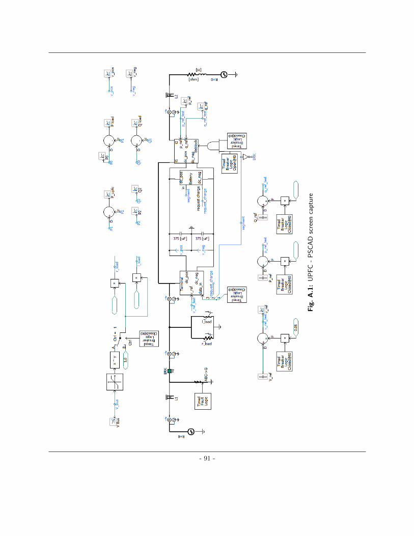
Fig.A.1:
UP
FC
-P
SC
AD
scre
enca
ptu
re
- 91 -

Fig. A.2: UPFC shunt - PSCAD screen capture
- 92 -

Fig.A.3:
UP
FC
seri
es-
PS
CA
Dsc
reen
cap
ture
- 93 -

Fig.A.4:
UP
FC
bat
tery
-P
SC
AD
scre
enca
ptu
re
- 94 -

B. Grid Energy Storage - Additional Details
Appendix B
Grid Energy Storage - Additional
Details
This appendix contains additional information on grid energy storage systems.
B.1 Available Storage Technology
There are a variety of technologies that can be used to store energy. These include but are not
limited to: pumped hydro, compressed air, batteries, flywheels, capacitors, etc. [6]. Each of these
has advantages and disadvantages depending on the application. Therefore some applications may
lend themselves better to one type of technology over another. In addition, some technologies have
specific site requirements which may limit where they can be constructed.
B.1.1 Pumped Hydro
Traditional hydro generation takes advantage of naturally occurring bodies of water in which the
water moves from a physically higher reservoir to a lower reservoir, such as a river. A dam is used
to direct water through a turbine which spins a generator such that the potential energy of the
- 95 -

B.1 Available Storage Technology
water is converted to electrical energy. This type of generation may have some inherent storage
capability. Energy storage is achieved by blocking the water and allowing it to pass through the
turbine at a later time. [7]. Pumped hydro storage combines traditional hydro generation with the
ability to pump the water back from the lower reservoir to the higher reservoir. This effectively
converts electricity back to potential energy in the water. This type of storage is geographically
limited since physical water and some form of reservoir are required [18].
Pumped hydro storage is one of the oldest and most well established forms of energy storage.
Capacity can range from hundreds to thousands of megawatt-hours and therefore pumped hydro
is well suited to large scale energy storage. Round trip efficiency for this type of storage is approx-
imately 80% [19] and the life span of pumped hydro plants is in the range of many decades [6].
Pumped hydro can be used for cost reduction in the form of peak shaving, or for reliability such
as backup power or smoothing renewable generation sources [20]. As of 2016, 98% of installed grid
level energy storage capacity world wide was in the form of pumped hydro storage [21].
B.1.2 Compressed air
Compressed air energy storage is also an old technology of energy storage. The concept is very
similar to pumped hydro in that air is pumped into a reservoir and then released through a turbine
at a later time to generate electricity. This process may require additional energy in the form of fuel
depending on the implementation. The reservoir used is often an underground geological feature
and therefore this technology is also geographically limited [22]. Compressed air is also suited for
large scale energy storage in the range of hundreds of megawatt-hours, but it does not boast the
same level of efficiency as pumped hydro. In theory, efficiency could be as high as 70% in a pure
storage application. However in practice, fossil fuels are required and actual efficiency (including
thermal efficiency associated with the fuel) is approximately 50% [23]. Applications for this type of
- 96 -

B.1 Available Storage Technology
storage are similar to pumped hydro: peak shaving, backup power, renewable generation smoothing,
etc [6].
B.1.3 Flywheels
A flywheel is a rotating mass in which energy is stored in the form of kinetic energy. Electricity
brings the mass up to speed at which point a converter can turn the kinetic energy back into
electrical energy. This type of storage has a fast response time and can be cycled nearly indefinitely
with no loss of capacity [24]. This type of storage is best suited to frequency control due to its fast
response time and relatively low energy capacity. There are no specific geological requirements for
this technology and therefore it can be deployed anywhere [6]. Currently flywheels have a small
capacity in the order of a few megawatt-hours. Flywheels are a relatively new technology and are
the subject of ongoing research [23].
B.1.4 Chemical
Chemical energy storage, more commonly called battery energy storage, is a form of electrochem-
ical storage where electrical energy is used to drive a chemical reaction that can be reversed to
extract some of the energy back. The merits of a battery are directly associated with its chemical
composition. Some of the commercially available chemistries are: Lead-acid, Lithium-Ion (Li-ion),
Sodium, and Redox Flow [23]. Battery capacity ranges from a few hundred kilowatt-hours to tens
of megawatt-hours depending on the chemistry [25]. Battery storage facilities have no geological
requirements and can be constructed almost anywhere. The wide range of capacity means that
batteries can be useful in a variety of applications. Li-ion batteries have high energy density but are
not as suited for extensive discharge and therefore lend themselves more to frequency management.
Sodium batteries can be discharged to a larger degree and for longer periods of time which makes
it more suitable for peak shaving or backup power. However, sodium batteries do not have as
- 97 -

B.1 Available Storage Technology
high of energy density. Lead-acid battery technology is the most mature and cheapest chemistry
but has the lowest energy density and therefore does not scale as easily. The low energy density
means that a utility scale battery would require more material to produce the batteries (i.e. either
physically larger or more numerous), resulting in a larger site requirement with more interfacing
infrastructure, all of which add cost [6].
The life span of a battery is possibly the biggest drawback of the technology. The capacity
of a battery is reduced over time as its chemical composition degrades and is not easily repaired.
This is affected by a large array of factors such as: cathode/anode material, operating temperature,
discharge current, charge current, depth of discharge, method of charge, method of discharge, etc.
For example, Li-ion batteries in an electric vehicle application can degrade to 80% of initial capacity
in anywhere from a few hundred to a few thousand cycles [26]. For comparison, a sodium-type
battery in a small scale application demonstrated a reduction in capacity to 80% after ten thousand
cycles [27].
• Lead-acid
Lead-acid batteries are perhaps the oldest commercially viable technology of battery. Working
examples of lead acid batteries have existed since the late 1800s [28]. At a minimum, a lead acid
battery requires a lead plate as the negative electrode and a lead-oxyide (PbO2) plate as the positive
electric. Both electrodes are submerged in sulfuric acid (H2SO4). When electrons are allowed to
flow from the negative plate to the positive plate, a reversible reaction occurs where both electrodes
react with the acid to produce water and PbSO4 which accumulates on both plates. When electrons
are forced back across the electrodes, the reaction reverses and the water and PbSO4 turns back
into the respective plate material [29].
Lead-acid batteries come in two main varieties. The first type is “Starting, Lighting, and
Ignition” or SLI type which is designed for high discharge current with low depth of discharge. The
- 98 -

B.1 Available Storage Technology
second type is referred to as “deep cycle” which is designed for high depth of discharge with low
discharge current. The battery must be constructed to accommodate the use type, and batteries
of one use type will not be compatible in an application requiring the other use type [30]. SLI
type lead-acid batteries are almost ubiquitous amongst conventional modern vehicles which use a
battery to start the vehicle’s engine and support auxiliary equipment within the vehicle [30]. Deep
cycle batteries are more often used in a stationary application for purposes such as Uninterruptible
Power Supply (UPS) or grid level energy storage. A UPS application will typically hold the state
of charge at maximum and only infrequently discharge. A grid level energy storage application
may hold the state of charge below maximum so that both charging and discharge are available as
required [30].
There are several advantages to lead-acid batteries. The primary advantage is that lead-acid
batteries are extremely low cost per unit energy to produce due to abundance of material and ease
of production. Lead is a relatively safe and inert material by comparison to alternative battery
materials. Lead-acid batteries are also highly recyclable. Approximately 98% of the material in
the battery is recyclable [28]. The primary disadvantage of lead-acid batteries is high weight which
results in low specific energy and specific power. In a stationary application such as grid energy
storage, high weight is less of a concern [28]. Lead-acid battery cycle life depends strongly on the
type of operation. Deep cycling results in a shorter cycle life of approximately 600 cycles [31].
Shallow cycling, where the battery is only partially discharged and subsequently recharged, and
particularly if the cycling occurs in the midrange of capacity (e.g. from 70% to 40%), can result
in much higher cycle life, potentially in excess of 1000 cycles [31]. In either case, however, this is
relatively low by comparison to other battery chemistries.
- 99 -

B.1 Available Storage Technology
• Lithium Ion
Lithium Ion (Li-ion) batteries rose to popularity in the late 20th century along with increasing
popularity of small household electronics such as watches, cameras, and toys. These electronics
were often intended to be portable and thus the desire was for lightweight, long lasting batteries.
Li-ion batteries were one response to this desire [32]. In large part, lithium batteries were the
catalyst which allowed the spread of cell phones. Since then, enormous amounts of money have
been spent to advance the state of lithium batteries. This has been particularly in response to
rising popularity of electric vehicles. In the vehicle application, the specific energy of the battery
is of primary importance since it directly determines the range and efficiency of the vehicle and
hence the vehicle’s practicality [33].
A Li-ion battery is constructed by having two different non-lithium lattice structures for the
positive and negative electrodes. The lithium ions move through an electrolyte between the two
electrodes. During charging, the positively charged lithium moves from the positive electrode to
the negative electrode and accumulates within the lattice structure while electrons flow through the
external circuit. This process is reversed during discharge [34]. Lithium battery cycle life depends
on the specific chemistry used and the mode of operation. Typically when used for deep cycling,
the cycle life is at least 1000 cycles and as high as 4000 cycles. The cycle life can be increased
further to many thousands of cycles through the use of partial cycling [35].
The major advantages of lithium ion batteries are: high cycle life, high specific power (ap-
proximately 1000-2000 W/kg), high specific energy (100-200 Wh/kg), and low self discharge rates
(1-10 %/month) [35]. These characteristics have made the lithium battery extremely popular for all
types of portable applications from hand held electronics to vehicles. Lithium batteries are also well
suited for stationary power systems applications due to lithium’s high performance. Lithium bat-
teries for stationary applications are available in a wide range of energy capacities from a few kWh
to many MWh. Applications include frequency regulation, backup power, and peak smoothing.
- 100 -

B.1 Available Storage Technology
The primary disadvantages when compared to other battery chemistries are as follows. Lithium
has a relatively high cost per unit energy capacity. Lithium is very temperature sensitive; it loses
capacity if allowed to become cold, and it degrades rapidly if allowed to overheat. Further, the
temperature at which it overheats is relatively low by comparison to other chemistries [35].
Lithium batteries can be recycled, however the process to recycle is somewhat challenging
since lithium is highly reactive. In addition, commonly used cathode materials such as nickel and
cobalt are toxic. Batteries must also be discharged prior to recycling since the energy contained in
the cells will be released in the recycling process. This can cause dangerous sparking or heating
and the byproducts of recycling are often flammable [36]. The recycling process is often energy
intensive and produces reduced quality materials. This in conjunction with the relatively low cost
by comparison of raw materials means there is very little financial incentive to perform recycling.
As such, there has been only moderate investment into recycling processes [35].
• Sodium Ion
Sodium batteries operate by using molten sodium as the anode and either molten sulfur or a
mixture of molten salt with metal halide as the cathode. The molten electrodes are separated by
an aluminum oxide electrolyte which selectively allows the passage of sodium ions. In the sodium-
sulfur battery, the sodium ions release electrons, pass through the electrolyte, and react with the
sulfur. In the sodium metal halide battery, again the sodium releases electrons and the ions pass
through the electrolyte to react with the halogen. In either case the reaction is reversible [37].
Both sodium-sulfur and sodium metal halide batteries have relatively high specific energy (at
least 100 Wh/kg) and extremely high cycle life of multiple thousands of deep cycles. Sodium-sulfur
has better specific energy and cycle by comparison to sodium metal halide, however, molten sulfur
is highly corrosive and can lead to corrosion of the electrolyte. Care must be taken to prevent this
[37].
- 101 -

B.1 Available Storage Technology
One of the major benefits of the sodium type battery is that the materials required in construc-
tion are all relatively common and thus low cost. This compensates for the lesser specific energy
and specific power ratings. Sodium batteries require liquid sodium and thus very high operating
temperatures in the range of at least 200◦C. High operating temperatures require additional ther-
mal insulation and therefore present difficulty to implement and potential danger to the user. If the
battery is allowed to cool below its operating temperature, the sodium solidifies and the battery
will stop conducting until the sodium is reheated and melted [35].
• Redox Flow
Redox flow batteries are a class of battery within which exists a variety of chemistries. There are
many combinations of anode, cathode, and electrolyte chemistries which have different modes of
operation and varying strengths and weaknesses. The chemistry generally can be selected to shift
the battery more towards either high energy or high power. Flow-type batteries consist of a cathode
material dissolved in a liquid electrolyte and stored in a tank, and similarly with the anode material
in a separate tank. The two solutions share the same electrolyte and are prevented from directly
interacting by a selectively permeable separating medium which passes only the electrolyte. The
cathode and anode materials cannot pass through the separator [38].
Redox flow batteries have some advantages compared to other batteries due to the nature of
their construction in addition to the selected chemistry. The construction allows for the major
advantage of flow-type batteries. The power rating depends mostly on the surface area of the
separator, and the energy rating depends mostly on the tank size used for storing the anode and
cathode. Therefore the energy capacity can be increased by increasing the tank size without
impacting the power rating. Additionally, this means that a single battery has effectively no limit
to maximum capacity since a larger tank can always be constructed. Similarly the power rating
can be increased by increasing the surface area of the separator without changing the tank size
- 102 -

B.1 Available Storage Technology
[38]. The ability to access the storage tanks also means that the battery can be “recharged”
without electricity by replacing the anode and cathode material. The battery is capable of very
fast response times and has high short term overload capability. Flow-type batteries can have very
low self-discharge rates. They also have very high cycle life, in the range of several thousand deep
cycles [23].
The disadvantage of this type of battery is that it requires significant supporting infrastructure
in the form of tanks and pumps and is therefore typically only suitable for stationary applications.
This type of battery also suffers from relatively low specific energy and low specific power. This
is partially made up for by the ease of increasing the overall ratings of a battery for both energy
and power [25]. Energy efficiency of this type of battery is relatively low by comparison to other
battery types [23].
Flow-type batteries are suitable for almost any stationary application since they can be built to
any power/energy specification, and have excellent dynamic characteristics. Suitable applications
include: backup power, peak shaving, frequency regulation, power quality, energy arbitrage, etc.
The technology is relatively new and not yet commercially mature [6].
- 103 -
Related Documents