© 2013, IJARCSSE All Rights Reserved Page | 991 Volume 3, Issue 4, April 2013 ISSN: 2277 128X International Journal of Advanced Research in Computer Science and Software Engineering Research Paper Available online at: www.ijarcsse.com Design and Performance Optimization of 8-Channel WDM System Arashid Ahmad Bhat Assistant Professor Deptt.of ECE BGSB University ,J & K, India. Anamika Basnotra * Dept. of ITTE ]BGSB University, J & K, India Nisha Sharma Deptt.of ITTE BGSB University, J& K, India Abstract—This paper focuses on design of an 8-channel WDM System and then optimizing its performance parameters. This paper also focuses on evaluation of dependencies of various performance evaluating parameters onto various system parameters. Thus evaluating optimum fiber length, Channel frequencies and frequency spacing.This paper also draws an effective comparison between Non-EDFA WDM system and an EDFA based WDM system. The system was simulated and analyzed with OPTISYSTEM9 Simulation Tool. Keywords—BER, EDFA Amplifiers, OSNR, WDM Dispersion, Wavelength Division Multiplexing I. INTRODUCTION In this digital era the communication demand has increased from previous eras due to introduction of new communication techniques. As we can see there is increase in clients day by day, so we need huge bandwidth and high speed networks to deliver good quality of service to clients. Fiber optics communication is one of the major communication systems in modern era, which meets up the above challenges. This utilizes different types of multiplexing techniques to maintain good quality of service without traffic, less complicated instruments with good utilization of available resources .Wavelength Division Multiplexing (WDM) is one of them with good efficiency. It is based on dynamic light-path allocation. Here we have to take into consideration the physical topology of the WDM network and the traffic. We have designed here an 8-channel WDM system and carried out detailed analysis to evaluate the dependencies of the performance evaluating parameters onto the various system parameters. II. WDM In optical communication, wavelength division multiplexing (WDM) is a technology which carries a number of optical carrier signals on a single fibre by using different wavelengths of laser light. This allows bidirectional communication over one standard fibre with in increased capacity. As optical network supports huge bandwidth; WDM network splits this into a number of small bandwidths optical channels. It allows multiple data stream to be transferred along a same fibre at the same time. A WDM system uses a number of multiplexers at the transmitter end, which multiplexes more than one optical signal onto a single fibre and de-multiplexers at the receiver to split them apart. Generally the transmitter consists of a laser and modulator. The light source generates an optical carrier signal at either fixed or a tuneable wavelength. The receiver consists of photodiode detector which converts an optical signal to electrical signal [1]. This new technology allows engineers to increase the capacity of network without laying more fibre. It has more security compared to other types of communication from tapping and also immune to crosstalk [2]. Fig. 1 Wavelength Division Multiplexing System III. WDM TYPES OF NETWORKS The optical network has huge bandwidth and capacity can be as high as 1000 times the entire RF spectrum. But this is not the case due to attenuation of signals, which is a function of its wavelength and some other fibre limitation factor like

Welcome message from author
This document is posted to help you gain knowledge. Please leave a comment to let me know what you think about it! Share it to your friends and learn new things together.
Transcript
© 2013, IJARCSSE All Rights Reserved Page | 991
Volume 3, Issue 4, April 2013 ISSN: 2277 128X
International Journal of Advanced Research in Computer Science and Software Engineering Research Paper Available online at: www.ijarcsse.com
Design and Performance Optimization of 8-Channel WDM System Arashid Ahmad Bhat
Assistant Professor Deptt.of ECE
BGSB University
,J & K, India.
Anamika Basnotra*
Dept. of ITTE
]BGSB University,
J & K, India
Nisha Sharma
Deptt.of ITTE
BGSB University,
J& K, India
Abstract—This paper focuses on design of an 8-channel WDM System and then optimizing its performance
parameters. This paper also focuses on evaluation of dependencies of various performance evaluating parameters
onto various system parameters. Thus evaluating optimum fiber length, Channel frequencies and frequency
spacing.This paper also draws an effective comparison between Non-EDFA WDM system and an EDFA based WDM
system. The system was simulated and analyzed with OPTISYSTEM9 Simulation Tool.
Keywords—BER, EDFA Amplifiers, OSNR, WDM Dispersion, Wavelength Division Multiplexing
I. INTRODUCTION
In this digital era the communication demand has increased from previous eras due to introduction of new
communication techniques. As we can see there is increase in clients day by day, so we need huge bandwidth and high
speed networks to deliver good quality of service to clients. Fiber optics communication is one of the major
communication systems in modern era, which meets up the above challenges. This utilizes different types of multiplexing
techniques to maintain good quality of service without traffic, less complicated instruments with good utilization of
available resources .Wavelength Division Multiplexing (WDM) is one of them with good efficiency. It is based on
dynamic light-path allocation. Here we have to take into consideration the physical topology of the WDM network and
the traffic. We have designed here an 8-channel WDM system and carried out detailed analysis to evaluate the
dependencies of the performance evaluating parameters onto the various system parameters.
II. WDM
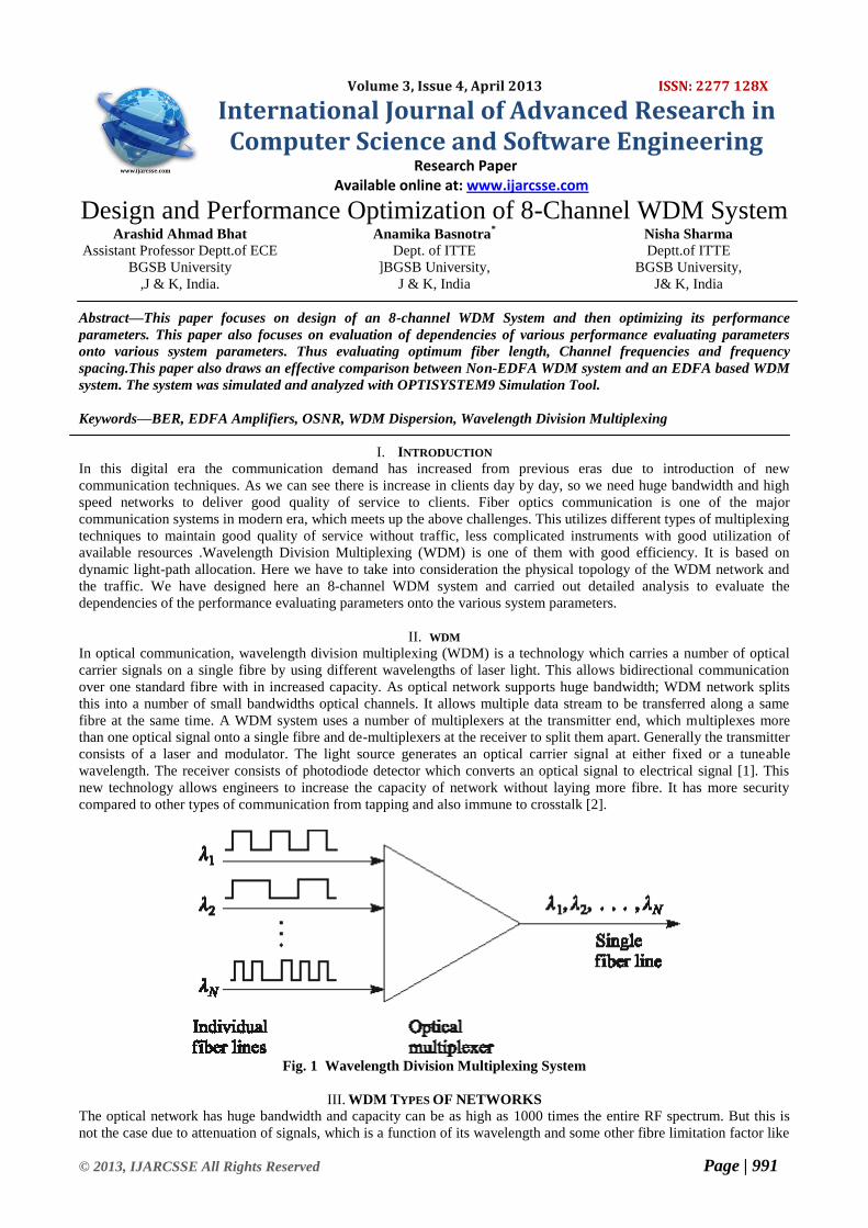
In optical communication, wavelength division multiplexing (WDM) is a technology which carries a number of optical
carrier signals on a single fibre by using different wavelengths of laser light. This allows bidirectional communication
over one standard fibre with in increased capacity. As optical network supports huge bandwidth; WDM network splits
this into a number of small bandwidths optical channels. It allows multiple data stream to be transferred along a same
fibre at the same time. A WDM system uses a number of multiplexers at the transmitter end, which multiplexes more
than one optical signal onto a single fibre and de-multiplexers at the receiver to split them apart. Generally the transmitter
consists of a laser and modulator. The light source generates an optical carrier signal at either fixed or a tuneable
wavelength. The receiver consists of photodiode detector which converts an optical signal to electrical signal [1]. This
new technology allows engineers to increase the capacity of network without laying more fibre. It has more security
compared to other types of communication from tapping and also immune to crosstalk [2].
Fig. 1 Wavelength Division Multiplexing System
III. WDM TYPES OF NETWORKS
The optical network has huge bandwidth and capacity can be as high as 1000 times the entire RF spectrum. But this is
not the case due to attenuation of signals, which is a function of its wavelength and some other fibre limitation factor like

Ahmad Bhat et al., International Journal of Advanced Research in Computer Science and Software Engineering 3(4),
April - 2013, pp. 991-1002
© 2013, IJARCSSE All Rights Reserved Page | 992
imperfection and refractive index fluctuation. So 1300nm (0.32dB/km)-1550nm (0.2dB/km) window with low
attenuation is generally used.
According to different wavelength pattern there are 3 existing types as:-
WDM (Wavelength Channel Multiplexing)
CWDM (Coarse Wavelength Division Multiplexing)
DWDM (Dense Wavelength Division Multiplexing)
Table1 Types of WDM Networks
Parameter WDM CWDM DWDM
Channel
Spacing
1310nm &
1550nm
Large,1.6nm-
25nm
Small,1.6nm or
less
No of base
bands used
C(1521-1560
nm)
S(1480-1520
nm)C(1521-
1560
nm),L(1561-
1620 nm)
C(1521-1560
nm),L(1561-
1620 nm
Cost per
Channel
Low Low High
No of
Channels
Delivered
2 17-18 most hundreds of
channel
possible
Best
application
PON Short haul,
Metro
Long Haul
III.WDM BENEFITS
Wavelength Channel Multiplexing (WDM) is important technology used in today’s telecommunication systems. It has
better features than other types of communication with client satisfaction. It has several benefits that make famous among
clients such as:
A. Capacity Upgrade
Communication using optical fibre provides very large bandwidth. Here the carrier for the data stream is light. Generally
a single light beam is used as the carries. But in WDM, lights having different wavelengths are multiplexed into a single
optical fibre. So in the same fibre now more data is transmitted. This increases the capacity of the network considerably
B. Transparency
WDM networks supports data to be transmitted at different bit rates. It also supports a number of protocols. So there is
not much constraint in how we want to send the data. So it can be used for various very high speed data transmission
applications.
C. Wavelength Reuse
WDM networks allows for wavelength routing. So in different fibre links the same wavelength can be used again and
again. This allows for wavelength reuse which in turn helps in increasing capacity [3].
D. Scalability
WDM networks are also very flexible in nature. As per requirement we can make changes to the network. Extra
processing units can be added to both transmitter and receiver ends. By this infrastructure can redevelop to serve more
number of people.
E. Reliability
WDM networks are extremely reliable and secure. Here chance of trapping the data and crosstalk is very low. It also can
recover from network failure in a very efficient manner. There is provision for rerouting a path between a source
destination node pair. So in case of link failure we will not lose any data [4].
IV.OPERATIONAL BLOCK DIAGRAM
The operational block diagram of a general WDM system is given below in Fig2
Fig. 2 Block Diagram of a general WDM System
Ahmad Bhat et al., International Journal of Advanced Research in Computer Science and Software Engineering 3(4),
April - 2013, pp. 991-1002
© 2013, IJARCSSE All Rights Reserved Page | 993
Here input data (Digitized) generated at different wavelengths is given to the input of a WDM multiplexer which
multiplexed them into a single data stream. This data after proper electro-opto conversion and external modulation is
transmitted to the desired length via single mode optical fiber. Proper amplification is provided by deployment of looped
EDFA amplifier with adequate gain. At reception the data streams are separated by WDM de-Mux and filtered to their
respective wavelengths after proper opto-electro conversion.
V. Performance Evaluating Parameters For Wdm System
The various parameters which give us a measure of how good or bad the transmission is are called as Performance
Evaluating parameters. The various Performance evaluating parameters are
Bit Error Rate (BER): In telecommunication transmission, the bit error rate (BER) is the percentage of bits that have
errors relative to the total number of bits received in a transmission, usually expressed as ten to a negative power.
Q-Factor: Physically speaking, Q is 2π times the ratio of the total energy stored divided by the energy lost in a single
cycle or equivalently the ratio of the stored energy to the energy dissipated per one radian of the oscillation. Equivalently,
it compares the frequency at which a system oscillates to the rate at which it dissipates its energy.
Eye Height: Eye diagrams show parametric information about the signal – effects deriving from physics such as system
bandwidth health, etc. It will not show protocol or logical problems – if logic 1 is healthy on the eye, this does not reveal
the fact that the system meant to send a zero. The height of such an eye diagram from bottom to top is called eye height
and is a performance evaluation component, the larger the eye height the better is the transmission.
OSNR: Optical Signal to Noise Ratio (OSNR) is defined as the ratio of optical signal power to the noise power within
the system. Higher the OSNR better is the signal reception.
VI. System Parameters
The various system parameters onto which the performance of the WDM system depends include Frequency Spacing
between adjacent channels, Fiber Length, EDFA Gain and operating Frequency of channels.
VII. Simulation Setup
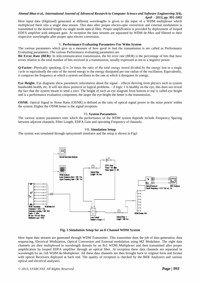
The system was simulated through optisystem9 simulator and the setup is shown in Fig3
Fig. 3 Simulation Setup for an 8-Channel WDM System
Here Input data streams are generated through WDM Transmitter. This transmitter does the job of data generation, data
sequencing, Electrical Modulation, Optical Conversion and External modulation using MZ Modulator. The eight data
channels are then multiplexed in wavelength domain by an 8x1 WDM Multiplexer and then transmitted after proper
amplification by looped EDFA amplifier through an optical fiber. At reception these data channels are separated in
wavelength by an 1x8 WDM de-Multiplexer. All these data channels are then brought back to original form and format
with optical Receivers deployed at back end. The quality of reception is checked by the BER Analyzers and various
optical and electrical analysers.
Ahmad Bhat et al., International Journal of Advanced Research in Computer Science and Software Engineering 3(4),
April - 2013, pp. 991-1002
© 2013, IJARCSSE All Rights Reserved Page | 994
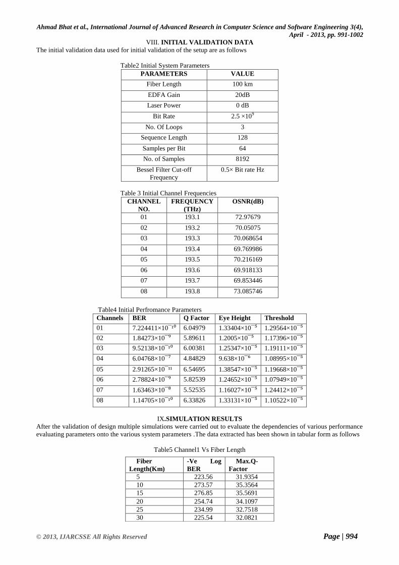
VIII. INITIAL VALIDATION DATA
The initial validation data used for initial validation of the setup are as follows
Table2 Initial System Parameters
PARAMETERS VALUE
Fiber Length 100 km
EDFA Gain 20dB
Laser Power 0 dB
Bit Rate 2.5 ×10⁹
No. Of Loops 3
Sequence Length 128
Samples per Bit 64
No. of Samples 8192
Bessel Filter Cut-off
Frequency
0.5× Bit rate Hz
Table 3 Initial Channel Frequencies
CHANNEL
NO.
FREQUENCY
(THz)
OSNR(dB)
01 193.1 72.97679
02 193.2 70.05075
03 193.3 70.068654
04 193.4 69.769986
05 193.5 70.216169
06 193.6 69.918133
07 193.7 69.853446
08 193.8 73.085746
Table4 Initial Perfromance Parameters
Channels BER Q Factor Eye Height Threshold
01 7.224411×10¯¹⁰ 6.04979 1.33404×10¯⁵ 1.29564×10¯⁵
02 1.84273×10¯⁹ 5.89611 1.2005×10¯⁵ 1.17396×10¯⁵
03 9.52138×10¯¹⁰ 6.00381 1.25347×10¯⁵ 1.19111×10¯⁵
04 6.04768×10¯⁷ 4.84829 9.638×10¯⁶ 1.08995×10¯⁵
05 2.91265×10¯¹¹ 6.54695 1.38547×10¯⁵ 1.19668×10¯⁵
06 2.78824×10¯⁹ 5.82539 1.24652×10¯⁵ 1.07949×10¯⁵
07 1.63463×10¯⁸ 5.52535 1.16027×10¯⁵ 1.24412×10¯⁵
08 1.14705×10¯¹⁰ 6.33826 1.33131×10¯⁵ 1.10522×10¯⁵
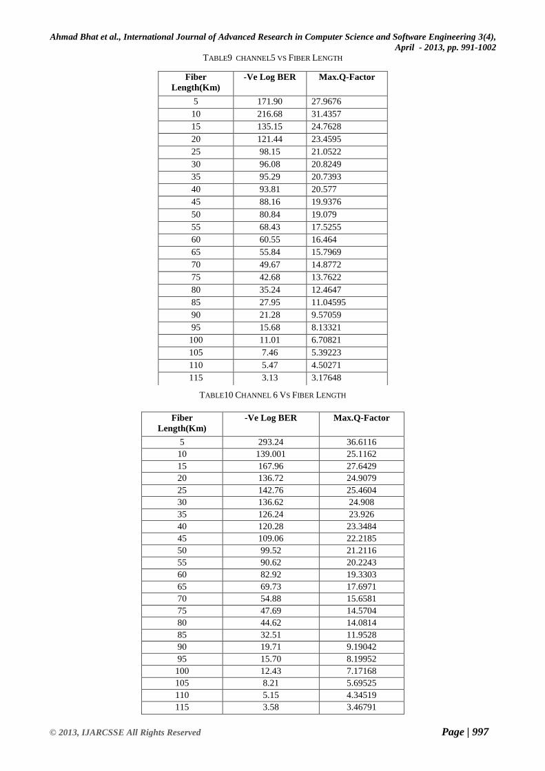
IX.SIMULATION RESULTS
After the validation of design multiple simulations were carried out to evaluate the dependencies of various performance
evaluating parameters onto the various system parameters .The data extracted has been shown in tabular form as follows
Table5 Channel1 Vs Fiber Length
Fiber
Length(Km)
-Ve Log
BER
Max.Q-
Factor
5 223.56 31.9354
10 273.57 35.3564
15 276.85 35.5691
20 254.74 34.1097
25 234.99 32.7518
30 225.54 32.0821

Ahmad Bhat et al., International Journal of Advanced Research in Computer Science and Software Engineering 3(4),
April - 2013, pp. 991-1002
© 2013, IJARCSSE All Rights Reserved Page | 995
TABLE6 CHANNEL2 VS FIBER LENGTH
Table7 channel3 vs fiber length
35 195.43 29.846
40 176.73 28.3692
45 148.92 26.0191
50 157.63 26.7776
55 117.90 23.1199
60 104.48 21.7445
65 88.11 19.9438
70 66.82 17.3223
75 56.25 15.8619
80 37.85 12.9357
85 32.50 11.9525
90 22.86 9.94237
95 17.44 8.61226
100 11.59 6.90343
105 6.15 4.82599
110 5.65 4.59146
115 3.38 3.34766
Fiber
Length(Km)
-Ve Log BER Max.Q-Factor
5 280.08 35.7755
10 239.37 33.0544
15 237.23 32.9058
20 239.25 33.0476
25 213.93 31.2356
30 219.57 31.6493
35 185.73 29.0885
40 180.57 28.6776
45 169.93 27.813
50 160.49 27.024
55 133.39 24.611
60 107.88 22.1023
65 91.47 20.3272
70 75.18 18.3975
75 80.43 19.0427
80 49.17 14.8047
85 31.66 11.7895
90 25.03 10.4263
95 16.35 8.31873
100 12.84 7.30006
105 7.09 5.23156
110 5.47 4.50271
115 3.72 3.5558
Fiber
Length(Km)
-Ve Log BER Max.Q-Factor
5 145.96 25.7458
10 193.37 29.6802
15 185.57 29.0693
20 177.64 28.4369
25 142.44 25.4329

Ahmad Bhat et al., International Journal of Advanced Research in Computer Science and Software Engineering 3(4),
April - 2013, pp. 991-1002
© 2013, IJARCSSE All Rights Reserved Page | 996
TABLE 8 CHANNEL4 VS FIBER LENGTH
30 155.04 26.5483
35 129.34 24.2222
40 111.22 23.4395
45 115.64 22.888
50 97.85 21.027
55 86.90 19.7981
60 70.85 17.8429
65 60.68 16.4845
70 56.99 15.9641
75 44.22 14.0115
80 34.74 12.369
85 25.86 10.6062
90 20.77 9.44832
95 12.73 7.26553
100 10.12 6.40351
105 7.07 5.23323
110 5.15 4.34519
115 3.10 3.15896
Fiber
Length(Km)
-Ve Log BER Max.Q-Factor
5 134.87 24.7347
10 81.04 19.0883
15 71.07 17.8494
20 58.67 16.1768
25 53.94 15.4941
30 49.15 14.7706
35 46.37 14.335
40 47.64 14.5401
45 47.94 14.5892
50 47.20 14.4723
55 46.94 14.4336
60 45.37 14.1796
65 40.85 13.4369
70 34.72 12.3538
75 28.98 11.2466
80 22.22 9.78307
85 16.53 8.35956
90 12.09 7.06072
95 9.84 6.3036
100 8.50 5.8108
105 6.90 5.15918
110 5.12 4.3303
115 3.70 3.54077
Ahmad Bhat et al., International Journal of Advanced Research in Computer Science and Software Engineering 3(4),
April - 2013, pp. 991-1002
© 2013, IJARCSSE All Rights Reserved Page | 997
TABLE9 CHANNEL5 VS FIBER LENGTH
TABLE10 CHANNEL 6 VS FIBER LENGTH
Fiber
Length(Km)
-Ve Log BER Max.Q-Factor
5 171.90 27.9676
10 216.68 31.4357
15 135.15 24.7628
20 121.44 23.4595
25 98.15 21.0522
30 96.08 20.8249
35 95.29 20.7393
40 93.81 20.577
45 88.16 19.9376
50 80.84 19.079
55 68.43 17.5255
60 60.55 16.464
65 55.84 15.7969
70 49.67 14.8772
75 42.68 13.7622
80 35.24 12.4647
85 27.95 11.04595
90 21.28 9.57059
95 15.68 8.13321
100 11.01 6.70821
105 7.46 5.39223
110 5.47 4.50271
115 3.13 3.17648
Fiber
Length(Km)
-Ve Log BER Max.Q-Factor
5 293.24 36.6116
10 139.001 25.1162
15 167.96 27.6429
20 136.72 24.9079
25 142.76 25.4604
30 136.62 24.908
35 126.24 23.926
40 120.28 23.3484
45 109.06 22.2185
50 99.52 21.2116
55 90.62 20.2243
60 82.92 19.3303
65 69.73 17.6971
70 54.88 15.6581
75 47.69 14.5704
80 44.62 14.0814
85 32.51 11.9528
90 19.71 9.19042
95 15.70 8.19952
100 12.43 7.17168
105 8.21 5.69525
110 5.15 4.34519
115 3.58 3.46791
Ahmad Bhat et al., International Journal of Advanced Research in Computer Science and Software Engineering 3(4),
April - 2013, pp. 991-1002
© 2013, IJARCSSE All Rights Reserved Page | 998
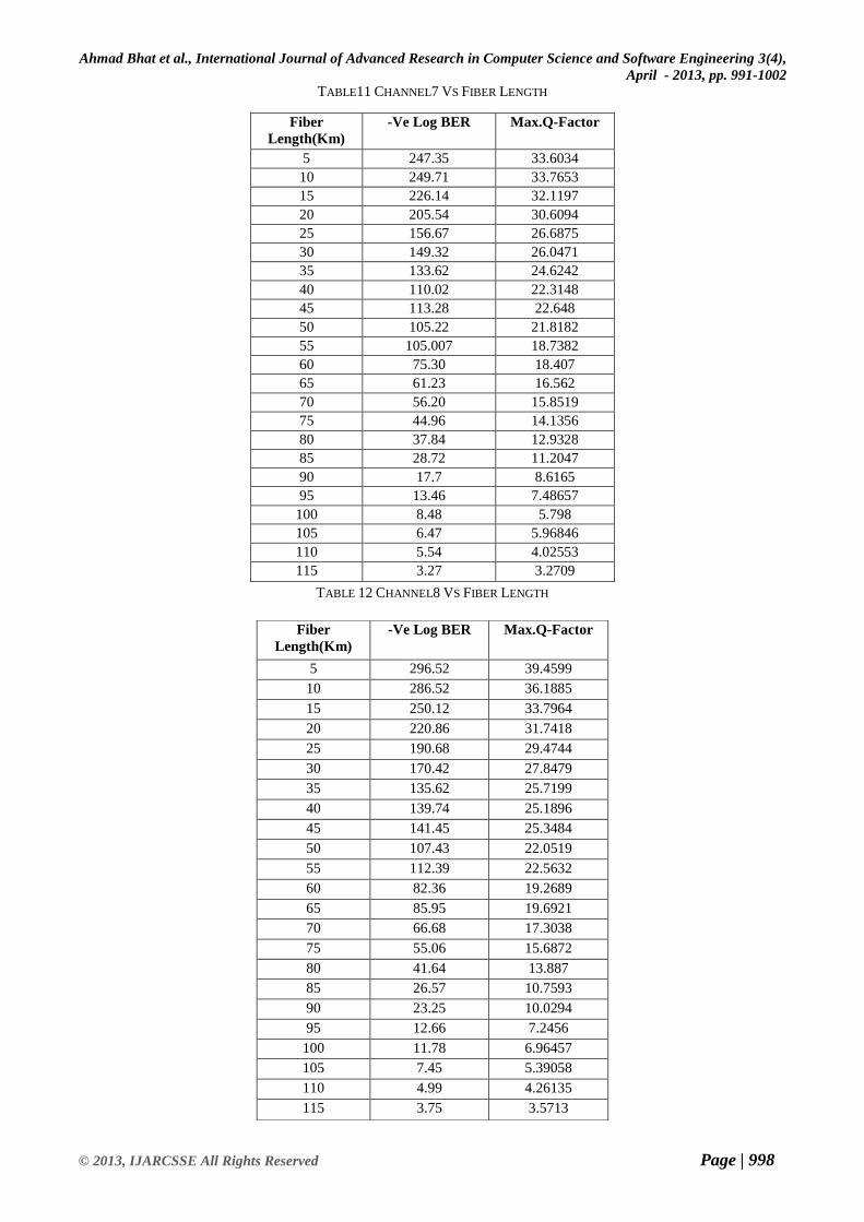
TABLE11 CHANNEL7 VS FIBER LENGTH
TABLE 12 CHANNEL8 VS FIBER LENGTH
Fiber
Length(Km)
-Ve Log BER Max.Q-Factor
5 247.35 33.6034
10 249.71 33.7653
15 226.14 32.1197
20 205.54 30.6094
25 156.67 26.6875
30 149.32 26.0471
35 133.62 24.6242
40 110.02 22.3148
45 113.28 22.648
50 105.22 21.8182
55 105.007 18.7382
60 75.30 18.407
65 61.23 16.562
70 56.20 15.8519
75 44.96 14.1356
80 37.84 12.9328
85 28.72 11.2047
90 17.7 8.6165
95 13.46 7.48657
100 8.48 5.798
105 6.47 5.96846
110 5.54 4.02553
115 3.27 3.2709
Fiber
Length(Km)
-Ve Log BER Max.Q-Factor
5 296.52 39.4599
10 286.52 36.1885
15 250.12 33.7964
20 220.86 31.7418
25 190.68 29.4744
30 170.42 27.8479
35 135.62 25.7199
40 139.74 25.1896
45 141.45 25.3484
50 107.43 22.0519
55 112.39 22.5632
60 82.36 19.2689
65 85.95 19.6921
70 66.68 17.3038
75 55.06 15.6872
80 41.64 13.887
85 26.57 10.7593
90 23.25 10.0294
95 12.66 7.2456
100 11.78 6.96457
105 7.45 5.39058
110 4.99 4.26135
115 3.75 3.5713
Ahmad Bhat et al., International Journal of Advanced Research in Computer Science and Software Engineering 3(4),
April - 2013, pp. 991-1002
© 2013, IJARCSSE All Rights Reserved Page | 999
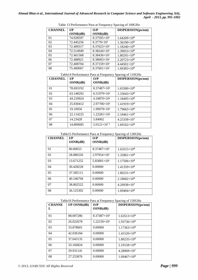
Table 13 Performance Para at Frequency Spacing of 100GHz
Table14 Performance Para at Frequency Spacing of 110GHz
CHANNEL I/P
OSNR(dB)
O/P
OSNR(dB)
DISPERSION(ps/nm)
01 78.693192 8.37487×10¹ 1.63580×10⁸
02 63.148292 6.51979×10¹ 1.33043×10⁸
03 44.210924 4.34870×10¹ 1.18495×10⁸
04 25.830412 2.97706×10¹ 1.41919×10⁸
05 19.10056 1.99079×10¹ 1.79665×10⁸
06 22.114225 1.22281×10¹ 2.18461×10⁸
07 14.23428 5.84062 4.25358×10⁷
08 14.800685 5.0121×10¯¹ 1.69162×10⁸
Table15 Performance Para at Frequency Spacing of 130GHz
CHANNEL I/P
OSNR(dB)
O/P
OSNR(dB)
DISPERSION(ps/nm)
01 80.80653 8.37487×10¹ 1.63515×10⁸
02 28.880226 2.97954×10¹ 1.32861×10⁸
03 13.671252 5.83081×10¹ 1.17506×10⁸
04 30.428228 0.00000 1.41359×10⁸
05 37.585111 0.00000 1.80231×10⁸
06 40.546794 0.00000 2.18682×10⁸
07 38.802522 0.00000 4.26938×10⁷
08 36.125302 0.00000 1.69404×10⁸
Table16 Performance Para at Frequency Spacing of 150GHz
CHANNE
L
I/P OSNR(dB) O/P
OSNR(dB)
DISPERSION(ps/nm)
01 88.007286 8.37487×10¹ 1.63513×10⁸
02 26.022678 1.22150×10¹ 1.93736×10⁸
03 33.878601 0.00000 1.17363×10⁸
04 42.036184 0.00000 1.41520×10⁸
05 37.043135 0.00000 1.80235×10⁸
06 33.166824 0.00000 2.19158×10⁸
07 29.931141 0.00000 4.28969×10⁷
08 27.253876 0.00000 1.69467×10⁸
CHANNEL I/P
OSNR(dB)
O/P
OSNR(dB)
DISPERSION(ps/nm)
01 74.928597 8.37595×10¹ 1.64209×10⁸
02 72.445256 8.3779×10¹ 1.36190×10⁸
03 72.409317 8.37623×10¹ 1.18240×10⁸
04 72.514949 8.38244×10¹ 1.39053×10⁸
05 72.461568 8.38436×10¹ 1.80291×10⁸
06 72.488921 8.38083×10¹ 2.20723×10⁸
07 72.408704 8.37159×10¹ 4.44501×10⁷
08 75.400067 8.37601×10¹ 1.69383×10⁸
Ahmad Bhat et al., International Journal of Advanced Research in Computer Science and Software Engineering 3(4),
April - 2013, pp. 991-1002
© 2013, IJARCSSE All Rights Reserved Page | 1000
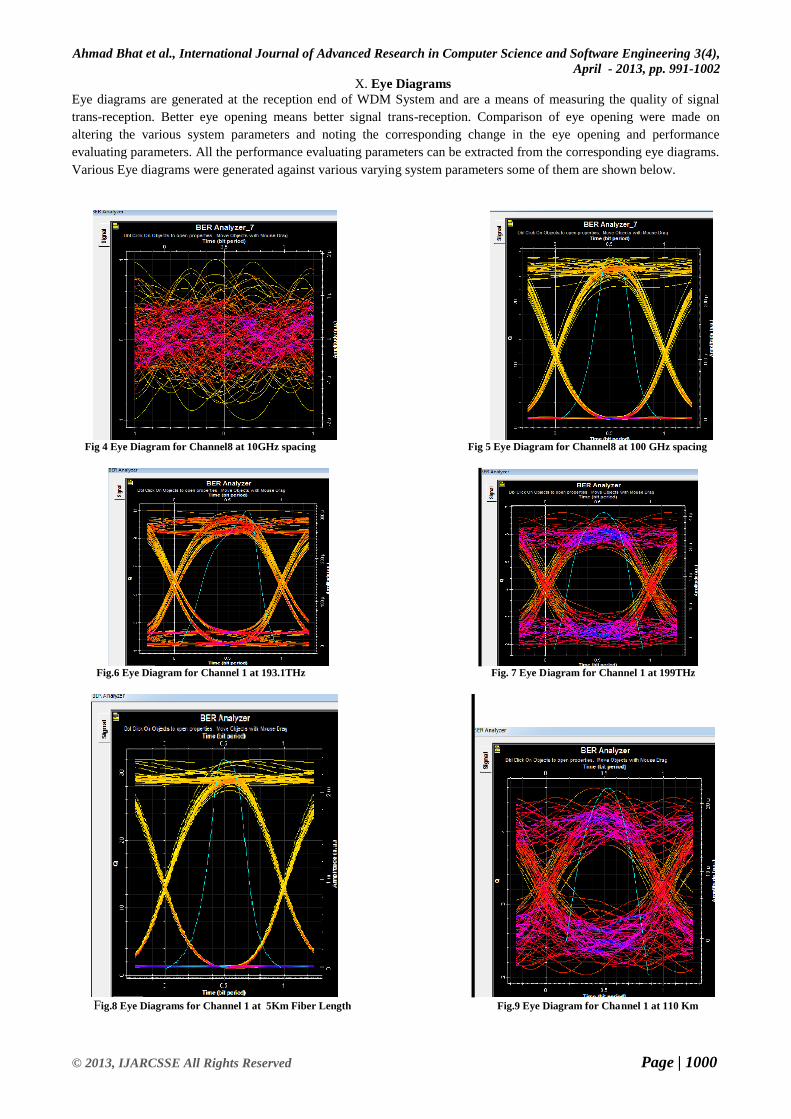
X. Eye Diagrams
Eye diagrams are generated at the reception end of WDM System and are a means of measuring the quality of signal
trans-reception. Better eye opening means better signal trans-reception. Comparison of eye opening were made on
altering the various system parameters and noting the corresponding change in the eye opening and performance
evaluating parameters. All the performance evaluating parameters can be extracted from the corresponding eye diagrams.
Various Eye diagrams were generated against various varying system parameters some of them are shown below.
Fig 4 Eye Diagram for Channel8 at 10GHz spacing Fig 5 Eye Diagram for Channel8 at 100 GHz spacing
Fig.6 Eye Diagram for Channel 1 at 193.1THz Fig. 7 Eye Diagram for Channel 1 at 199THz
Fig.8 Eye Diagrams for Channel 1 at 5Km Fiber Length Fig.9 Eye Diagram for Channel 1 at 110 Km
Ahmad Bhat et al., International Journal of Advanced Research in Computer Science and Software Engineering 3(4),
April - 2013, pp. 991-1002
© 2013, IJARCSSE All Rights Reserved Page | 1001
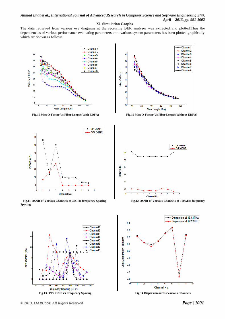
XI. Simulation Graphs
The data retrieved from various eye diagrams at the receiving BER analyser was extracted and plotted.Thus the
dependencies of various performance evaluating parameters onto various system parameters has been plotted graphically
which are shown as follows
Fig.10 Max Q-Factor Vs Fiber Length(With EDFA) Fig.10 Max Q-Factor Vs Fiber Length(Without EDFA)
Fig.11 OSNR of Various Channels at 30GHz frequency Spacing Fig.12 OSNR of Various Channels at 100GHz frequency
Spacing
Fig.13 O/P OSNR Vs Frequency Spacing Fig.14 Dispersion across Various Channels
Ahmad Bhat et al., International Journal of Advanced Research in Computer Science and Software Engineering 3(4),
April - 2013, pp. 991-1002
© 2013, IJARCSSE All Rights Reserved Page | 1002
XII. Discussions From Graphs
From the above graphs it was observed that
A. BER Increases with Fiber length,and maximum fiber length which the system could support was found out to be 110
Kms with EDFA and 90 Kms without EDFA
B.OSNR of all channels dropped as the frequency spacing was reduced and best OSNR was seen around frequency
spacing of 100GHz.
C. Difference between I/P OSNR and O/P OSNR was seen minimum when operated at frequency spacing of around
100GHz
D. Dispersion first increased reached a maximum and then decreased to reach a minimum (Channel7) at channel
frequency set at 193.8 THz.
XIII.Conclusion
Here the dependencies of various performance evaluating parameters i.e. Min.BER, Max. Q-Factor, Eye Opening,
Dispersion and OSNR on various system parameters i.e. Fiber length, Operating Channel Frequencies, Adjacent channel
spacing , and EDFA gain were evaluated .The obtained results were found in well accordance with real results.
REFERENCES
[1] Jun Zheng & Hussein T.Mouftah, Optical WDM networks, concepts and Design, IEEE press, John Wiley –
Sons, Inc., Publication, p.1-4, 2004.
[2] R. Ramaswami, K.N. Sivarajan, “Optical Networks-A Practical Perspective, Second Edition, Morgan Kaufmann
-Publishers An Imprint Of Elsevier , New Delhi, India, 2004
[3] G. Ramesh, S. Sundaravadivelu, “Reliable Routing and Wavelength Assignment Algorithm for Optical WDM
Networks”, European Journal of Scientific Research ISSN 1450-216X Vol.48 No.1, 2010.
[4] A.S. Acampora,” A multichannel multihop local light wave net-work”, Proceedings, IEEE Globecom’87,
Tokyo, Japan, Vol.3, 1987
Related Documents


