HAL Id: tel-01165064 https://tel.archives-ouvertes.fr/tel-01165064 Submitted on 18 Jun 2015 HAL is a multi-disciplinary open access archive for the deposit and dissemination of sci- entific research documents, whether they are pub- lished or not. The documents may come from teaching and research institutions in France or abroad, or from public or private research centers. L’archive ouverte pluridisciplinaire HAL, est destinée au dépôt et à la diffusion de documents scientifiques de niveau recherche, publiés ou non, émanant des établissements d’enseignement et de recherche français ou étrangers, des laboratoires publics ou privés. Design and optimization of wireless backhaul networks Alvinice Kodjo To cite this version: Alvinice Kodjo. Design and optimization of wireless backhaul networks. Other [cs.OH]. Université Nice Sophia Antipolis, 2014. English. NNT : 2014NICE4140. tel-01165064

Welcome message from author
This document is posted to help you gain knowledge. Please leave a comment to let me know what you think about it! Share it to your friends and learn new things together.
Transcript
HAL Id: tel-01165064https://tel.archives-ouvertes.fr/tel-01165064
Submitted on 18 Jun 2015
HAL is a multi-disciplinary open accessarchive for the deposit and dissemination of sci-entific research documents, whether they are pub-lished or not. The documents may come fromteaching and research institutions in France orabroad, or from public or private research centers.
L’archive ouverte pluridisciplinaire HAL, estdestinée au dépôt et à la diffusion de documentsscientifiques de niveau recherche, publiés ou non,émanant des établissements d’enseignement et derecherche français ou étrangers, des laboratoirespublics ou privés.
Design and optimization of wireless backhaul networksAlvinice Kodjo
To cite this version:Alvinice Kodjo. Design and optimization of wireless backhaul networks. Other [cs.OH]. UniversitéNice Sophia Antipolis, 2014. English. �NNT : 2014NICE4140�. �tel-01165064�
UNIVERSITÉ DE NICE - SOPHIA ANTIPOLISÉCOLE DOCTORALE DES SCIENCES ET TECHNOLOGIES DE
L’INFORMATION ET DE LA COMMUNICATION
THÈSEpour obtenir le titre de
Docteur en Sciencesde l’Université de Nice - Sophia Antipolis
Mention : Informatique
Présentée par
Alvinice KODJOTitre français
Dimensionnement et optimisation desréseaux de collecte sans fil
Equipe projet COATIINRIA, I3S (CNRS/UNS)
Thèse dirigée parDavid Coudert - COATI (INRIA, I3S (CNRS/UNS))
Soutenance le 18 Décembre 2014
Jury:
Président: Philippe Michelon - LIA (Avignon, France)Rapporteurs: Hervé Rivano - INRIA (Lyon, France)
Dritan Nace - UTC (Compiègne, France)Examinators: Brigitte Jaumard - CSE - UC (Montréal, Canada)
Patrick Beatini - 3ROAM (Sophia Antipolis, France)


Acknowledgements
I would not have been able to arrive at the end of this thesis without the support andthe encouragements of several people. I want to take this opportunity to sincerelythank them.
My heartfelt thanks to my advisor Dr David Coudert for all the confidence heplaced in me throughout these years. He was always available to discuss with mewhen I was lost and provided me precious advices for solving my difficult problems.I also thank him for for the great patience he showed during the review of mymanuscript.
I would like to thank Pr Dritan Nace and Dr Hervé Rivano who accepted toreview my thesis. Their comments and suggestions helped me to provide clearexplanations on essential elements of my thesis.
I am also thankful to all my co-authors without whom I would not certainly haveobtained such qualities of results. It was a pleasure and a good experience for meto work with all of them. A special thanks to Pr Brigitte Jaumard who welcomedme in her team during a month in Montreal and who also agreed to be a memberof my jury. I learnt a lot by working with her and I am grateful for the excellentexample she has provided me as researcher and teacher.
I thank all the current and past members of the Mascotte/Coati team thanksto who it was always a pleasure to come to work. Thank you for pleasant momentsshared together. My thanks also go to all my friends from Ubinet and Inria. Onethousand thanks to Patricia Lachaume for the friendship and the kindness whichshe always showed with me. She is a very beautiful and a great lady I can neverforget.
My life in Nice and Sophia would have been rather solitary without the presenceof the members of the Bisso family. Thank you infinitely for the love, the friendshipand the support during all this period.
To my dear Aminath Badarou who is more than a friend, I want to sincerelythank you for everything you have done for me in my life. She understands mebetter than anyone and always has the right words to confort me. We still have alot to share.
I would like to express my infinite gratitude and my love to my dear parents, mybrothers and sisters. Thank you Mom and Dad for your support and your prayers.You sacrificed a lot so I can be the woman I am today and I cannot thank youenough for that. A big thank to my sisters and brother for always being present bymy side.
Finally, I dedicate this thesis to my lovely son Leroy-Jethro who is and willforever be the main engine of my life.

iii
Résumé
L’essentiel des travaux de cette thèse porte sur les réseaux de collectes de donnéessans fil. Ce type de réseaux présente l’avantage de permettre un déploiement facileet rapide à des coûts relativement faibles tout en offrant des capacités pouvantaller jusqu’à 1Gbps sur des liens d’une centaine de kilomètres. Nous avons étudiédifférents problèmes d’optimisation dans ces réseaux qui représentent de vrais chal-lenges pour les industriels du secteur.
Le premier problème porte sur l’allocation de capacités sur les liens à coût min-imum. Il a été résolu par une approche de programmation linéaire avec générationde colonnes. Notre modèle permet de résoudre des problèmes de grandes tailles. Deplus, nous obtenons rapidement des solutions de très bonnes qualités.
Nous avons ensuite étudié le problème du partage d’infrastructure réseau entreopérateurs virtuels. L’objectif est alors de maximiser les revenus de l’opérateurde l’infrastructure physique tout en satisfaisant les demandes et les contraintes dequalité de service des opérateurs virtuels clients du réseau. Dans ce contexte, nousavons proposé une modélisation du problème en programmation linéaire en nombresentiers mixte. Notre formulation est robuste aux variations de trafic des opérateursvirtuels.
Un autre point de dépenses dans ce type de réseau est la consommation d’énergie.De nombreux opérateurs cherchent aujourd’hui à réduire la consommation d’énergiedes réseaux, à la fois en utilisant des équipements plus performants et en utilisantdes solutions de routage plus adaptées. Nous avons proposé une solution robuste, deroutage basée sur la consommation d’energie du réseau. Le modèle proposé est basésur les réseaux backbone mais il devrait être assez aisément adaptable aux réseauxde collectes sans fil. Notre solution a été formulée en utilisant un programme linéaireen nombre entiers mixte. Nous avons aussi proposé des heuristiques afin de trouverassez rapidement des solutions pour de grandes instances.
Le dernier travail de cette thèse porte sur les réseaux radio cognitifs et plusprécisément sur le problème de partage de bande passante. Nous l’avons formaliséen utilisant un programme linéaire mais avec une autre approche d’optimisationrobuste. Ce modèle diffère des autres cas d’optimization robuste abordé plus hautpar la position des termes incertains du modèle. Pour la résolution, nous noussommes basés sur la formulation linéaire à 2-niveaux proposé par Michel Minoux.
Cette thèse a été effectuée en partenariat avec la PME 3ROAM ((http://www.3roam.com) et en collaboration avec différents chercheurs de diverses universitésdans le monde. Elle a été co-financée par la région PACA et la PME 3ROAM.
iv
Abstract
The main work of this thesis focuses on the wireless backhaul networks. This type ofnetwork has the advantage of allowing rapid and easy deployment at relatively lowcosts while offering capacity of up to 1Gbps over links of a hundred of kilometers.We studied different optimization problems in such networks that represent realchallenges for industrial sector.
The first issue addressed in Chapter 3 focuses on the capacity allocation on thelinks at minimum cost. It was solved by a linear programming approach with columngeneration. Our method solves the problems on large size networks. In addition, wequickly obtain very good quality solutions.
We then studied the problem of network infrastructure sharing between virtualoperators. The objective is to maximize the revenue of the operator of the physicalinfrastructure while satisfying the demands (constraints of quality of service) ofvirtual operators customers of the network. In this context, we proposed a modelto the problem using mixed integer linear programming. Our formulation is robustto changes in traffic demands of virtual operators.
Another operational expenditure in this type of network is the energy consump-tion. Many operators are now seeking to reduce network energy consumption, bothby using more efficient equipments and by using more appropriate routing solutions.We proposed a robust energy-aware routing solution for the network. The proposedmodel is based on backbone networks, but it can easily be adapted to wireless back-haul networks. Our solution was formulated using a mixed integer linear program.We also proposed heuristics to find efficient solutions for large networks.
The last work of this thesis focuses on cognitive radio networks and more specifi-cally on the problem of bandwidth sharing. We formalized it using a linear programwith a different approach to robust optimization. This model differs from other casesof robust optimization discussed above by the position of the uncertain terms in themodel. We based our solution on the 2-stage linear robust formulation proposed byMichel Minoux.
This thesis was carried out in partnership with the SME 3ROAM (http://www.3roam.com) and in collaboration with various researchers from different universitiesin the world. It was co-funded by the PACA province and the SME 3ROAM.
Contents
1 Introduction 11.1 Motivation and Context . . . . . . . . . . . . . . . . . . . . . . . . . 11.2 Broadband Wireless Access technologies . . . . . . . . . . . . . . . . 41.3 Dimensioning and dynamic routing in Backhaul Networks . . . . . . 71.4 Routing real fluctuated traffic in microwave wireless networks . . . . 81.5 Energy saving . . . . . . . . . . . . . . . . . . . . . . . . . . . . . . . 81.6 Tools and Techniques . . . . . . . . . . . . . . . . . . . . . . . . . . . 91.7 Thesis Organization and Contributions . . . . . . . . . . . . . . . . . 101.8 List of publications . . . . . . . . . . . . . . . . . . . . . . . . . . . . 11
2 Preliminaries 132.1 Linear Programming . . . . . . . . . . . . . . . . . . . . . . . . . . . 132.2 Column generation . . . . . . . . . . . . . . . . . . . . . . . . . . . . 152.3 Robust optimization . . . . . . . . . . . . . . . . . . . . . . . . . . . 16
2.3.1 Γ−robustness . . . . . . . . . . . . . . . . . . . . . . . . . . . 172.3.2 2-stage Robust LP with RHS uncertainty . . . . . . . . . . . 18
2.4 Introduction to the Optimization Programming Language, OPL . . . 19
3 Dimensioning of Microwave Wireless Networks 233.1 Introduction . . . . . . . . . . . . . . . . . . . . . . . . . . . . . . . . 243.2 Related Work . . . . . . . . . . . . . . . . . . . . . . . . . . . . . . . 25
3.2.1 Literature Review . . . . . . . . . . . . . . . . . . . . . . . . 253.2.2 Budget Constrained Optimization Model . . . . . . . . . . . . 25
3.3 Network Model . . . . . . . . . . . . . . . . . . . . . . . . . . . . . . 273.3.1 Definitions and Assumptions . . . . . . . . . . . . . . . . . . 283.3.2 Problem formulation . . . . . . . . . . . . . . . . . . . . . . . 283.3.3 An Illustrative Example . . . . . . . . . . . . . . . . . . . . . 30
3.4 Solution of the Model . . . . . . . . . . . . . . . . . . . . . . . . . . 313.4.1 The Random Column Enumeration (RCE) heuristic . . . . . 343.4.2 The Modified Column Generation (MCG) heuristic . . . . . . 353.4.3 Initial Solution of the RMP . . . . . . . . . . . . . . . . . . . 36
3.5 Numerical Results . . . . . . . . . . . . . . . . . . . . . . . . . . . . 373.5.1 Resolution process . . . . . . . . . . . . . . . . . . . . . . . . 383.5.2 Solution quality . . . . . . . . . . . . . . . . . . . . . . . . . . 383.5.3 Validation of the Results: Comparison with those of [CKCN14] 40
3.6 Conclusion . . . . . . . . . . . . . . . . . . . . . . . . . . . . . . . . . 40
vi Contents
4 Infrastructure sharing 434.1 Introduction . . . . . . . . . . . . . . . . . . . . . . . . . . . . . . . . 434.2 Problem definition and nominal formulation . . . . . . . . . . . . . . 46
4.2.1 Problem situation . . . . . . . . . . . . . . . . . . . . . . . . 464.2.2 Static model formulation . . . . . . . . . . . . . . . . . . . . . 46
4.3 Robust model . . . . . . . . . . . . . . . . . . . . . . . . . . . . . . . 484.4 Computational results . . . . . . . . . . . . . . . . . . . . . . . . . . 50
4.4.1 Computation settings and test instances . . . . . . . . . . . . 504.4.2 Results and discussion . . . . . . . . . . . . . . . . . . . . . . 51
4.5 Model limits . . . . . . . . . . . . . . . . . . . . . . . . . . . . . . . . 564.6 Heuristics . . . . . . . . . . . . . . . . . . . . . . . . . . . . . . . . . 57
4.6.1 Powerset method . . . . . . . . . . . . . . . . . . . . . . . . . 574.6.2 Nominal-based method . . . . . . . . . . . . . . . . . . . . . . 574.6.3 Greedy method . . . . . . . . . . . . . . . . . . . . . . . . . . 594.6.4 Heuristics performance . . . . . . . . . . . . . . . . . . . . . . 59
4.7 Conclusion . . . . . . . . . . . . . . . . . . . . . . . . . . . . . . . . . 62
5 Energy-aware Routing in Backbone Networks 635.1 Context and motivation . . . . . . . . . . . . . . . . . . . . . . . . . 645.2 Related Works . . . . . . . . . . . . . . . . . . . . . . . . . . . . . . 66
5.2.1 Energy-aware Routing (EAR) . . . . . . . . . . . . . . . . . . 665.2.2 Redundancy Elimination . . . . . . . . . . . . . . . . . . . . . 685.2.3 GreenRE - Energy Savings with Redundancy Elimination . . 69
5.3 Robust-GreenRE Model . . . . . . . . . . . . . . . . . . . . . . . . . 725.3.1 Compact formulation . . . . . . . . . . . . . . . . . . . . . . . 755.3.2 Constraint generation (Exact Algorithm) . . . . . . . . . . . 765.3.3 Heuristic Algorithm . . . . . . . . . . . . . . . . . . . . . . . 78
5.4 Computational Evaluation . . . . . . . . . . . . . . . . . . . . . . . . 805.4.1 Test instances and Experimental settings . . . . . . . . . . . 805.4.2 Results and Discussion . . . . . . . . . . . . . . . . . . . . . . 81
5.5 Conclusion . . . . . . . . . . . . . . . . . . . . . . . . . . . . . . . . . 89
6 Conclusion 91
A Optimization in Cognitive Radio Networks 93A.1 Cognitive Radio Networks . . . . . . . . . . . . . . . . . . . . . . . . 94A.2 Related works and problem definition . . . . . . . . . . . . . . . . . . 95A.3 Nominal model . . . . . . . . . . . . . . . . . . . . . . . . . . . . . . 98A.4 Robust model . . . . . . . . . . . . . . . . . . . . . . . . . . . . . . 99A.5 Conclusion . . . . . . . . . . . . . . . . . . . . . . . . . . . . . . . . . 103
B Résumé des Travaux de thèse 105B.1 Contexte et motivation . . . . . . . . . . . . . . . . . . . . . . . . . . 105B.2 Les technologies d’accès à haut débit . . . . . . . . . . . . . . . . . . 108
Contents vii
B.3 Dimensionnement et routage dynamique dans les réseaux de collecteà micro ondes . . . . . . . . . . . . . . . . . . . . . . . . . . . . . . . 112
B.4 Routage des requêtes de volumes variables dans les réseaux de collecteà micro ondes . . . . . . . . . . . . . . . . . . . . . . . . . . . . . . . 113
B.5 Les économies d’énergie . . . . . . . . . . . . . . . . . . . . . . . . . 114B.6 Nos contributions . . . . . . . . . . . . . . . . . . . . . . . . . . . . . 115B.7 Liste des publications . . . . . . . . . . . . . . . . . . . . . . . . . . 121B.8 Conclusion . . . . . . . . . . . . . . . . . . . . . . . . . . . . . . . . . 121
Bibliography 123

List of Figures
1.1 Example of Wireless backhaul network . . . . . . . . . . . . . . . . . 21.2 Global microwave market [HR09] . . . . . . . . . . . . . . . . . . . . 31.3 Forecast backhaul connections in Europe [Obs10] . . . . . . . . . . . 41.4 Microwave link components . . . . . . . . . . . . . . . . . . . . . . . 6
2.1 Column generation algorithm flowchart . . . . . . . . . . . . . . . . . 172.2 OPL program of Example 2.1.1 . . . . . . . . . . . . . . . . . . . . . 22
3.1 Column Generation Process . . . . . . . . . . . . . . . . . . . . . . . 323.2 MCG Process . . . . . . . . . . . . . . . . . . . . . . . . . . . . . . . 363.3 Cost saving vs. the worst case . . . . . . . . . . . . . . . . . . . . . . 393.4 Reliability vs. the worst case . . . . . . . . . . . . . . . . . . . . . . 39
4.1 Example of fixed broadband wireless network . . . . . . . . . . . . . 444.2 Traffic demands in Abilene network [KKR13] . . . . . . . . . . . . . 494.3 Evolution of the revenus (4.3a), number of satisfied VNOs (4.3b), and
total number of satisfied demands (4.3c) as a function of Γ. . . . . . 524.4 Repartition of satisfied demands per VNO when Γ increases for Abi-
lene, Atlanta, and Polska. . . . . . . . . . . . . . . . . . . . . . . . . 534.5 Repartition of satisfied demand per VNO for Dfn. . . . . . . . . . . . 534.6 Evolution of the revenue (4.6a) and number of satisfied demands
(4.6b) on Dfn instance for different values of β and Γ. . . . . . . . . 544.7 Dfn instance with three VNOs such that |D1| = 65 = R1, |D2| =
25 = R2, and |D3| = 20 = R3. . . . . . . . . . . . . . . . . . . . . . . 554.8 Resolution performance comparison with Γ = 5 . . . . . . . . . . . . 614.9 Resolution performance comparison with Γ = 7 . . . . . . . . . . . . 62
5.1 Energy profiles . . . . . . . . . . . . . . . . . . . . . . . . . . . . . . 665.2 Example of Shortest Path Routing (SPR) vs. Energy-aware Routing
(EAR) . . . . . . . . . . . . . . . . . . . . . . . . . . . . . . . . . . . 675.3 Reduction of end-to-end link load using WOC . . . . . . . . . . . . . 685.4 GreenRE with 50% of traffic redundancy . . . . . . . . . . . . . . . . 695.5 Example of robustness . . . . . . . . . . . . . . . . . . . . . . . . . . 725.6 Diagram of constraint generation method . . . . . . . . . . . . . . . 765.7 Example of iterations of the CG method . . . . . . . . . . . . . . . . 785.8 Routing and RE-router placement on Abilene network . . . . . . . . 815.9 Upper bound and lower bound: Compact Formulation (CF) vs. Con-
straint Generation (CG) . . . . . . . . . . . . . . . . . . . . . . . . . 835.10 Optimality gaps: Compact Formulation (CF) vs. Constraint Gener-
ation (CG) . . . . . . . . . . . . . . . . . . . . . . . . . . . . . . . . 84
x List of Figures
5.11 Comparison of proposed methods on Abilene. . . . . . . . . . . . . . 855.12 Energy savings vs. robustness for Abilene, Geant and Germany50
network . . . . . . . . . . . . . . . . . . . . . . . . . . . . . . . . . . 865.13 CDF load of all links including links in sleep mode for Abilene, Geant
and Germany50 networks. . . . . . . . . . . . . . . . . . . . . . . . . 885.14 Robust-GreenRE vs. GreenRE vs. EAR. . . . . . . . . . . . . . . . . 89
A.1 Cognitive radio Network architecture [ALVM06] . . . . . . . . . . . . 95A.2 A CRN instance . . . . . . . . . . . . . . . . . . . . . . . . . . . . . 97A.3 Constraint generation process . . . . . . . . . . . . . . . . . . . . . . 103
B.1 Exemple d’un réseau de collecte sans fil . . . . . . . . . . . . . . . . 106B.2 Marché globale des liaisons à micro ondes [HR09] . . . . . . . . . . . 107B.3 Evolution et prévisions du nombre de liaisons des réseaux de collecte
en Europe [Obs10] . . . . . . . . . . . . . . . . . . . . . . . . . . . . 108B.4 Composants d’un lien à micro ondes . . . . . . . . . . . . . . . . . . 111B.5 Le processus d’exécution du MCG . . . . . . . . . . . . . . . . . . . 117B.6 Gain energétique vs. robustesse pour Abilene, Geant et Germany50
network . . . . . . . . . . . . . . . . . . . . . . . . . . . . . . . . . . 120B.7 Robust-GreenRE vs. GreenRE vs. EAR. . . . . . . . . . . . . . . . . 120
List of Tables
3.1 Modulation discrete probability distributions . . . . . . . . . . . . . 313.2 Configurations for z`1,b1 = z`2,b1 = z`3,b1 = 1 . . . . . . . . . . . . . . 313.3 Modulation schemes and Bandwidth efficiency . . . . . . . . . . . . . 373.4 CG Results . . . . . . . . . . . . . . . . . . . . . . . . . . . . . . . . 383.5 Resolution time (minutes) . . . . . . . . . . . . . . . . . . . . . . . . 40
4.1 Test instances settings . . . . . . . . . . . . . . . . . . . . . . . . . . 514.2 Dfn results in function of Γ . . . . . . . . . . . . . . . . . . . . . . . 554.3 Resolution time in seconds as function of Γ . . . . . . . . . . . . . . 56
5.1 Demands and redundancy rates variation . . . . . . . . . . . . . . . . 735.2 9 cases of the robustness . . . . . . . . . . . . . . . . . . . . . . . . . 735.3 Constraint Generation (CG) vs. Compact Formulation (CF) vs.
Heuristic for Abilene network. . . . . . . . . . . . . . . . . . . . . . . 82

Chapter 1
Introduction
Contents1.1 Motivation and Context . . . . . . . . . . . . . . . . . . . . . 1
1.2 Broadband Wireless Access technologies . . . . . . . . . . . 4
1.3 Dimensioning and dynamic routing in Backhaul Networks . 7
1.4 Routing real fluctuated traffic in microwave wireless networks 8
1.5 Energy saving . . . . . . . . . . . . . . . . . . . . . . . . . . . . 8
1.6 Tools and Techniques . . . . . . . . . . . . . . . . . . . . . . . 9
1.7 Thesis Organization and Contributions . . . . . . . . . . . . 10
1.8 List of publications . . . . . . . . . . . . . . . . . . . . . . . . 11
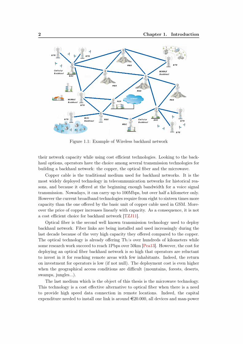
As the use of broadband services via mobile internet devices such as smartphonescontinues to grow, network operators have to regularly upgrade their network capac-ity to meet customers expectations. Among the available technologies, microwaveappears as a cost-effective transmission solution for extending the network cover-age and for providing bandwidth-intensive services to customers located in remoteareas.In this thesis, we study multiple optimization problems related to the cost-effectiveness of fixed microwave backhaul networks. The backhaul network can bedefined as the portion of the network infrastructure that provides interconnectionbetween the base station and the core network (see Fig. 1.1). In this chapter we firstmotivate the context of our work and then present the available broadband wirelesstechnologies. Finally, we briefly define the problems we studied, we introduce themethodologies used to solve them and we conclude this chapter by presenting ourcontributions and the thesis organisation.
1.1 Motivation and Context
The advent of broadband services (high definition TV, Voice over IP, Video OnDemand) has generated a rapid growth in data traffic, and consequently the needfor higher data bandwidth. Due to this growth, "Backhauling" that means "gettingdata to the backbone", has become a central challenge for network operators. Notonly do the operators need to improve customers experience, but they also have togenerate sufficient revenues with regard to their capital and operational expendi-tures. To solve this problem, operators have to install infrastructures that improve
2 Chapter 1. Introduction
Figure 1.1: Example of Wireless backhaul network
their network capacity while using cost efficient technologies. Looking to the back-haul options, operators have the choice among several transmission technologies forbuilding a backhaul network: the copper, the optical fiber and the microwave.
Copper cable is the traditional medium used for backhaul networks. It is themost widely deployed technology in telecommunication networks for historical rea-sons, and because it offered at the beginning enough bandwidth for a voice signaltransmission. Nowadays, it can carry up to 100Mbps, but over half a kilometer only.However the current broadband technologies require from eight to sixteen times morecapacity than the one offered by the basic unit of copper cable used in GSM. More-over the price of copper increases linearly with capacity. As a consequence, it is nota cost efficient choice for backhaul network [TZJ11].
Optical fiber is the second well known transmission technology used to deploybackhaul network. Fiber links are being installed and used increasingly during thelast decade because of the very high capacity they offered compared to the copper.The optical technology is already offering Tb/s over hundreds of kilometers whilesome research work succeed to reach 1Pbps over 50km [Pea13]. However, the cost fordeploying an optical fiber backhaul network is so high that operators are reluctantto invest in it for reaching remote areas with few inhabitants. Indeed, the returnon investment for operators is low (if not null). The deployment cost is even higherwhen the geographical access conditions are difficult (mountains, forests, deserts,swamps, jungles...).
The last medium which is the object of this thesis is the microwave technology.This technology is a cost effective alternative to optical fiber when there is a needto provide high speed data connection in remote locations. Indeed, the capitalexpenditure needed to install one link is around e20.000, all devices and man-power
1.1. Motivation and Context 3
included. The operational cost varies from one country to another. For instance,the cost for renting the frequency and the bandwidth for establishing one link inFrance ranges between e1.000 and e5.000 per year. This technology enables thedeployment of point-to-point communication links (with clear line-of-sight) with abit rate of up to 1Gbps between sites at distance up to 100km. It is therefore avery good choice for reaching remote locations, and so extending the coverage of anetwork operator.
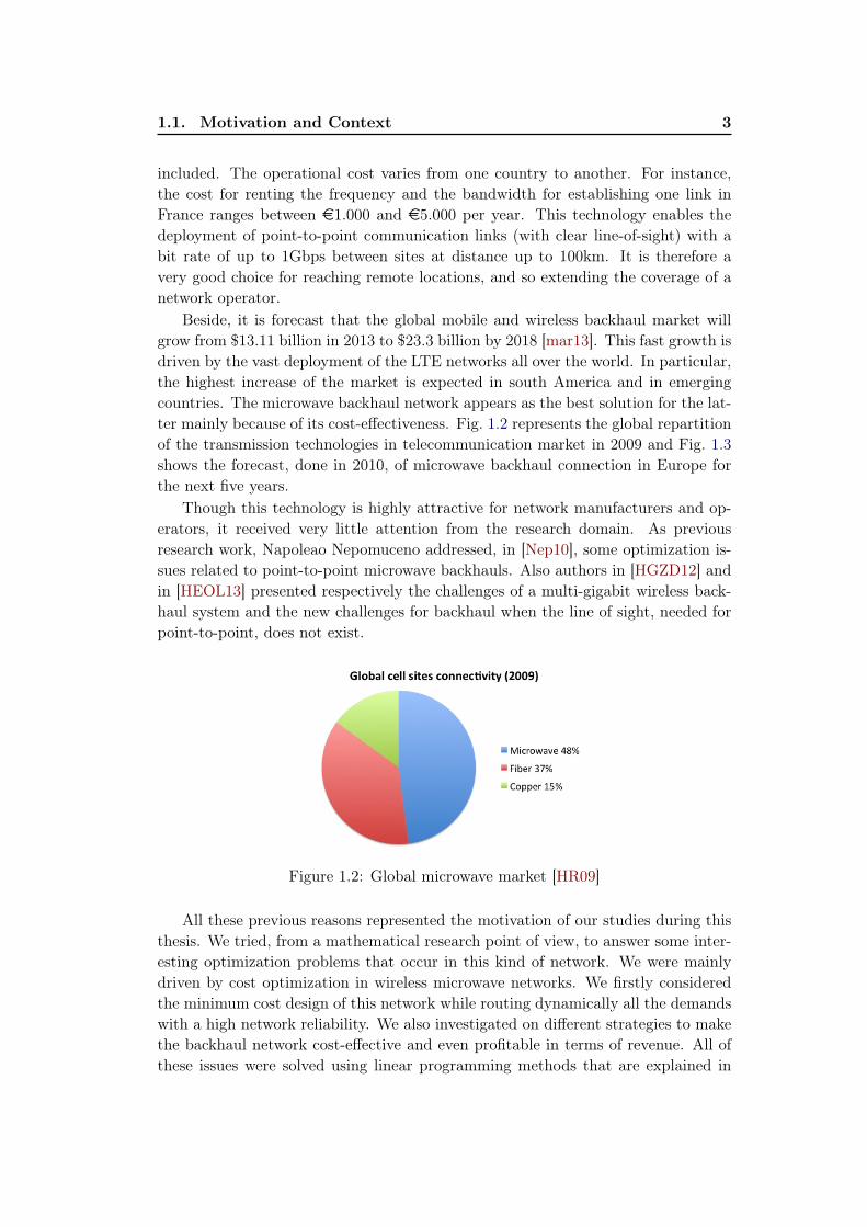
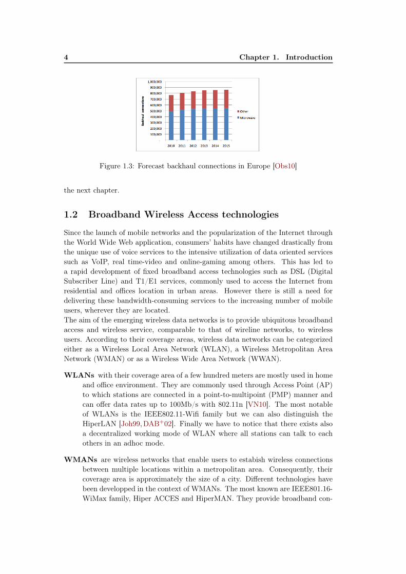
Beside, it is forecast that the global mobile and wireless backhaul market willgrow from $13.11 billion in 2013 to $23.3 billion by 2018 [mar13]. This fast growth isdriven by the vast deployment of the LTE networks all over the world. In particular,the highest increase of the market is expected in south America and in emergingcountries. The microwave backhaul network appears as the best solution for the lat-ter mainly because of its cost-effectiveness. Fig. 1.2 represents the global repartitionof the transmission technologies in telecommunication market in 2009 and Fig. 1.3shows the forecast, done in 2010, of microwave backhaul connection in Europe forthe next five years.
Though this technology is highly attractive for network manufacturers and op-erators, it received very little attention from the research domain. As previousresearch work, Napoleao Nepomuceno addressed, in [Nep10], some optimization is-sues related to point-to-point microwave backhauls. Also authors in [HGZD12] andin [HEOL13] presented respectively the challenges of a multi-gigabit wireless back-haul system and the new challenges for backhaul when the line of sight, needed forpoint-to-point, does not exist.
Figure 1.2: Global microwave market [HR09]
All these previous reasons represented the motivation of our studies during thisthesis. We tried, from a mathematical research point of view, to answer some inter-esting optimization problems that occur in this kind of network. We were mainlydriven by cost optimization in wireless microwave networks. We firstly consideredthe minimum cost design of this network while routing dynamically all the demandswith a high network reliability. We also investigated on different strategies to makethe backhaul network cost-effective and even profitable in terms of revenue. All ofthese issues were solved using linear programming methods that are explained in
4 Chapter 1. Introduction
Figure 1.3: Forecast backhaul connections in Europe [Obs10]
the next chapter.
1.2 Broadband Wireless Access technologies
Since the launch of mobile networks and the popularization of the Internet throughthe World Wide Web application, consumers’ habits have changed drastically fromthe unique use of voice services to the intensive utilization of data oriented servicessuch as VoIP, real time-video and online-gaming among others. This has led toa rapid development of fixed broadband access technologies such as DSL (DigitalSubscriber Line) and T1/E1 services, commonly used to access the Internet fromresidential and offices location in urban areas. However there is still a need fordelivering these bandwidth-consuming services to the increasing number of mobileusers, wherever they are located.The aim of the emerging wireless data networks is to provide ubiquitous broadbandaccess and wireless service, comparable to that of wireline networks, to wirelessusers. According to their coverage areas, wireless data networks can be categorizedeither as a Wireless Local Area Network (WLAN), a Wireless Metropolitan AreaNetwork (WMAN) or as a Wireless Wide Area Network (WWAN).
WLANs with their coverage area of a few hundred meters are mostly used in homeand office environment. They are commonly used through Access Point (AP)to which stations are connected in a point-to-multipoint (PMP) manner andcan offer data rates up to 100Mb/s with 802.11n [VN10]. The most notableof WLANs is the IEEE802.11-Wifi family but we can also distinguish theHiperLAN [Joh99,DAB+02]. Finally we have to notice that there exists alsoa decentralized working mode of WLAN where all stations can talk to eachothers in an adhoc mode.
WMANs are wireless networks that enable users to estabish wireless connectionsbetween multiple locations within a metropolitan area. Consequently, theircoverage area is approximately the size of a city. Different technologies havebeen developped in the context of WMANs. The most known are IEEE801.16-WiMax family, Hiper ACCES and HiperMAN. They provide broadband con-
1.2. Broadband Wireless Access technologies 5
nectivity to fixed, LOS (Line Of Sight), NLOS (Non-LOS) but also mobilesubscribers. They are based on cells covered using Base Station (BS) to whichSubscriber Stations (SS), that can be buildings or vehicles, are connected. Amesh topology mode is also supported by WMANs. WiMax helps to providean aggregate data raw rate of up to 135Mb/s based on the modulation used inLOS communication, while up to 75Mb/s is offered in NLOS communication,and HiperMAN can support up to 25Mb/s for each sector of an AP. Moretechnical details about these technologies are available in [KT07].
WWANs are commonly used to connect multiple WMANs located in physicallydistant areas. They mainly consist in satellite systems used principally inthe downlink way. Another WWAN technology developped is the IEEE802.20known as the Mobile Broadband Wireless Network (MBWA). The main goalof MBWA is to provide broadband access to highly mobile devices moving ata speed of up to 250km/h [BXG07] (in a car, a train, etc.).
Data from/to multiple WLANs can be aggregated and transmitted over aWMAN to the Internet and WWAN can help to interconnect different WMANscovering different areas. Beside these previous technologies, mobile technologiessuch as 3G (UMTS, HSPA, CDMA200, EV-DO) and 4G (LTE, LTE-Advanced)systems are also considered as broadband wireless access networks since they arenowadays providing high mobile data rates for their customers. They offer peakdata rates up to 14,4 Mb/s to mobile devices. All of these technologies are trans-mitting data through the air using radio frequencies (RF). In the context of ourresearch, we focused on the WMANs. More precisely, we studied problems relatedto a WMAN subnetwork that uses point-to-point (PtP) microwaves links to connectBase Stations (BSs) together and to route data traffic through the Internet or thebackbone network.
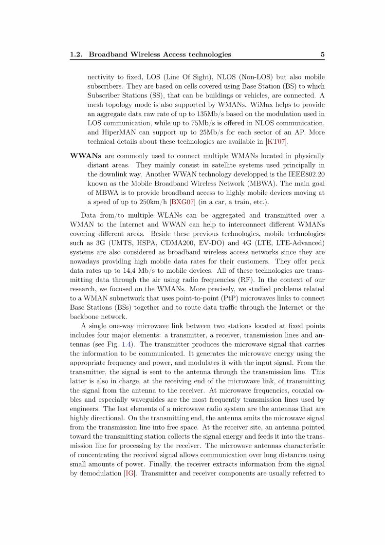
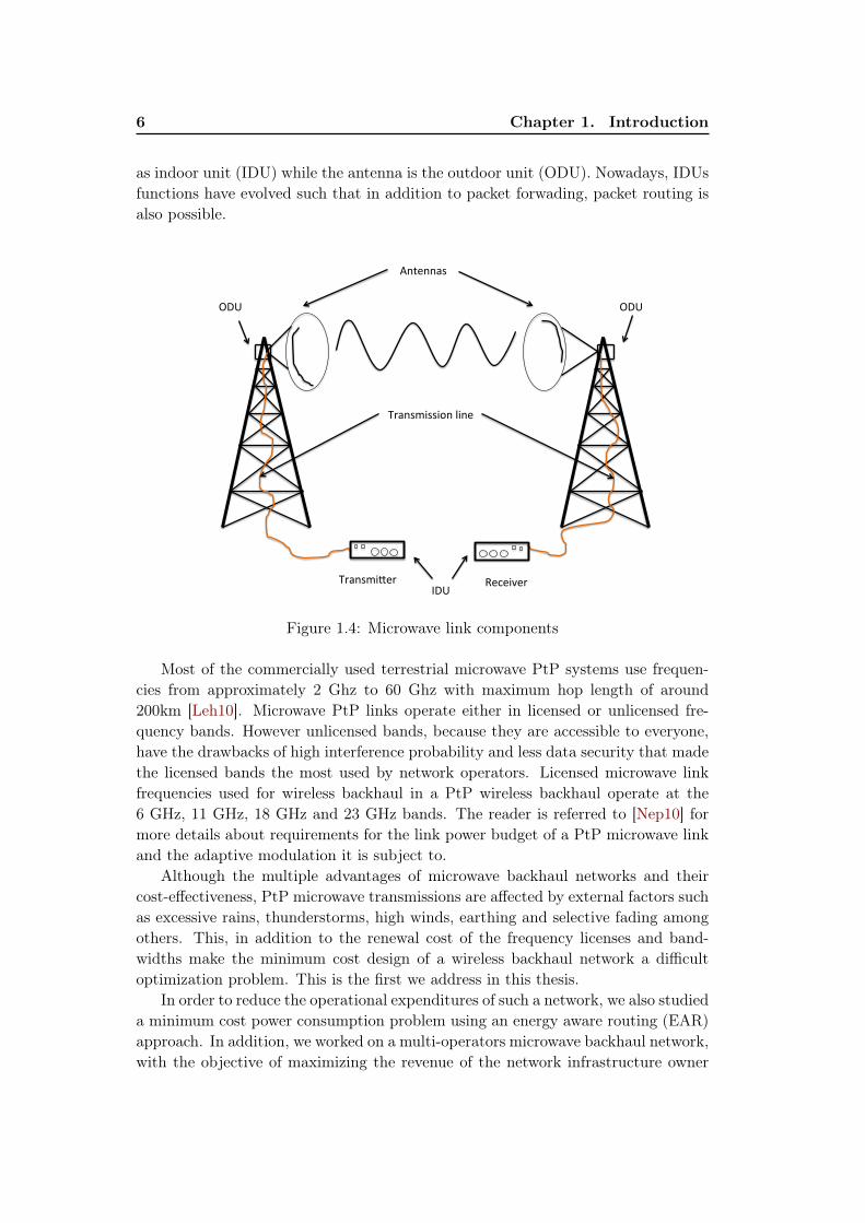
A single one-way microwave link between two stations located at fixed pointsincludes four major elements: a transmitter, a receiver, transmission lines and an-tennas (see Fig. 1.4). The transmitter produces the microwave signal that carriesthe information to be communicated. It generates the microwave energy using theappropriate frequency and power, and modulates it with the input signal. From thetransmitter, the signal is sent to the antenna through the transmission line. Thislatter is also in charge, at the receiving end of the microwave link, of transmittingthe signal from the antenna to the receiver. At microwave frequencies, coaxial ca-bles and especially waveguides are the most frequently transmission lines used byengineers. The last elements of a microwave radio system are the antennas that arehighly directional. On the transmitting end, the antenna emits the microwave signalfrom the transmission line into free space. At the receiver site, an antenna pointedtoward the transmitting station collects the signal energy and feeds it into the trans-mission line for processing by the receiver. The microwave antennas characteristicof concentrating the received signal allows communication over long distances usingsmall amounts of power. Finally, the receiver extracts information from the signalby demodulation [IG]. Transmitter and receiver components are usually referred to
6 Chapter 1. Introduction
as indoor unit (IDU) while the antenna is the outdoor unit (ODU). Nowadays, IDUsfunctions have evolved such that in addition to packet forwading, packet routing isalso possible.
Transmi(er Receiver
Antennas
Transmission line
ODU ODU
IDU
Figure 1.4: Microwave link components
Most of the commercially used terrestrial microwave PtP systems use frequen-cies from approximately 2 Ghz to 60 Ghz with maximum hop length of around200km [Leh10]. Microwave PtP links operate either in licensed or unlicensed fre-quency bands. However unlicensed bands, because they are accessible to everyone,have the drawbacks of high interference probability and less data security that madethe licensed bands the most used by network operators. Licensed microwave linkfrequencies used for wireless backhaul in a PtP wireless backhaul operate at the6 GHz, 11 GHz, 18 GHz and 23 GHz bands. The reader is referred to [Nep10] formore details about requirements for the link power budget of a PtP microwave linkand the adaptive modulation it is subject to.
Although the multiple advantages of microwave backhaul networks and theircost-effectiveness, PtP microwave transmissions are affected by external factors suchas excessive rains, thunderstorms, high winds, earthing and selective fading amongothers. This, in addition to the renewal cost of the frequency licenses and band-widths make the minimum cost design of a wireless backhaul network a difficultoptimization problem. This is the first we address in this thesis.
In order to reduce the operational expenditures of such a network, we also studieda minimum cost power consumption problem using an energy aware routing (EAR)approach. In addition, we worked on a multi-operators microwave backhaul network,with the objective of maximizing the revenue of the network infrastructure owner
1.3. Dimensioning and dynamic routing in Backhaul Networks 7
with respect to the demand satisfaction constraints. In this problem, we consideredtraffic volumes that vary in time and different quality of service (QoS) policy foreach network operator. These different problems are properly explained in the nextsections.
1.3 Dimensioning and dynamic routing in Backhaul Net-works
For any network operator or service provider, the main goal is to maximizeits revenue while ensuring the satisfaction of its customers. In the context oftelecommunication networks, in order to meet the needs of clients and offer thema good quality of experience, one of the key elements is to have a network withsufficient capacity on its links. Network operators should thus design their networkssuch that enough capacities are available on links to serve all clients needs anywhereand at anytime. For microwave backhaul network, this requirement has a centralplace since the base stations traffic needs have to be fully met. Otherwise the datathat have to be transported will either be delayed or lost. The capacity allocationon microwave network links is closely related to the efficient utilisation of the radiofrequency spectrum ressource. However this resource is limited and regulated, andthus expensive. The challenge here is then to cost-efficiently provide sufficientcapacity in order to meet customer satisfaction. From a technical point of view, todetermine the capacity of a microwave link, we need to know the channel bandwidthB and the modulation scheme m-QAM used to transmit data, with QAM standingfor Quadratic Adaptative Modulation. We use the following formula to calculatethe capacity:
Capacity[bps] = n.B[Hz] where n = log2 m
While the modulation scheme used in microwave radio systems is based on theadaptative modulation system, the bandwidth assignment on each link is a networkengineer’s decision. In fact, the adaptative modulation system refers to the au-tomatic modulation adjustment that a wireless system can make to prevent someweather-related fading. It has been developped mainly to help the radio network toadapt itself in bad transmission context in order to meet the bit error rate (BER)requirements. To reduce the total cost of bandwidths license renewal fees on thewhole network, there is a difficult optimization problem to be solved by the en-gineer at the network planning step. The main constraint of this problem is tosatisfy all the traffic demands. This constraint corresponds to the satisfaction ofthe well-known multi-commodities flow (MCF) problem [GCF99,Tom66,BCGT98].The MCF problem consists in routing commodities (here data traffic) from theirsources to their sinks through a given network with respect to the capacity of thelinks. The minimum cost bandwidth assignment problem, with the constraint ofhigh network reliability, was studied by Napoleão Nepomuceno in his thesis [Nep10]using a chance-constrained programming method.
8 Chapter 1. Introduction
Unlike the work of Nepomuceno, in this thesis we solved this problem whenconsidering a dynamic routing of demands. This differs from the previous workin the static data routing they have adopted. We also modeled the problem suchthat the solution is scalable and applicable to large networks (hundreds of links).This work, done in collaboration with David Coudert, Brigitte Jaumard (Concor-dia University, Canada), Mejdi Kaddour (Oran University, Algeria) and NapoleãoNepomuceno (Fortaleza University, Brazil), involves the utilization of mixed integerlinear programs (MILP) through a column generation method as well as a localsearch algorithm. Chapter 3 is devoted to the resolution of this problem.
1.4 Routing real fluctuated traffic in microwave wirelessnetworks
As pointed out previously, microwave backhaul network represents an attractivesolution for telecom operators and wireless Internet service providers to offer highspeed data rate to customers living in rural environment. However, it may not becost-effective for a network operator to fully deploy its own infrastructure, espe-cially when the number of targeted customers is small. An idea to overcome thisdifficulty is to share the network infrastructure among several network operatorsaiming at covering the same geographical area. This strategy is also recommendedby national telecommunications regulatory authorities for an efficient use of theradio spectrum among multiples operators. In this infrastructure sharing context,with the assumption that the network is already designed, we first investigated therevenue maximization problem for the network infrastructure owner. This objectivewas subject to the constraint of satisfying the maximum demands for each virtualnetwork operator with respect to their respective QoS policy. We then took in con-sideration the uncertainty of traffic demands to make the problem as realistic aspossible. To tackle this problem, we firstly propose an integer linear program (ILP)and a robust optimization method to handle the uncertainty factor. This problem,solved in collaboration with David Coudert and Christelle Caillouet (University ofNice Sophia Antipolis) is detailed in Chapter 4 of this thesis.
1.5 Energy saving
In the search for cost optimization strategies for backhaul networks, power con-sumption has been identified as a non-negligeable portion of operators operationalexpenditures (OPEX). In 2011, Tombaz et al have reported in [TMW+11], basedon [PVD+08], that 0,5% of the global energy is consumed by mobile communicationand around 80% of the power consumption in the mobile networks stems from theradio access network, namely radio base stations. With the installation of a largernumber of base stations required to satisfy the ever-increasing traffic demand, thisnumber is expected to double by 2020. This makes power consumption one of themajor issues to address by network operators especially in order to reduce their
1.6. Tools and Techniques 9
OPEX. It is mentionned in the Next Generation Mobile Networks optimised back-haul requirement [All08, requirement R88], that different consumption modes shouldbe available so that backhaul hadwares could automatically switch to the one withlowest power consumption. The idea, for backhaul network operators is then to finda solution to adapt their energy consumption to their traffic, in such a way thatunused base stations consume as few energy as possible.
The same problem also occurs in the Internet core network. Based on recentstudies, the power consumption of Internet’s infrastructure is estimated to be be-tween 1.1% and 1.9% of the 16 TW used by the humanity [BAH+09,RM11,BHT11,HBF+11]. In [TBA+08], authors identify that most Internet energy is consumed byaccess network and routers. They also state that this consumption will increase toover 4% as the access rate increases and that IP routers will be the energy bottleneckof the Internet.A proposal to limit this energy consumption growth is to use energy aware routing(EAR) [CSB+08, CMN09, BCRR12]. So together with Truong Khoa Phan, previ-ously PhD student in the Coati team, we decided to investigate this problem in thecontext of backbone networks. Our main objective was to minimize the total energyconsumption of the network under some specific constraints. Based on Phan’s previ-ous works [GMPR12,CKPT13], the problem was first tackled using EAR combinedto the so called Redundancy Elimination (RE) technique [AGA+08,ZCM11,ZA14].Then, using the robust optimization method, we extended the formulation intro-ducing some uncertainty on the traffic demand. Linear programs, a heuristic andan exact algorithms were developed to solve this problem. We present this work inChapter 5 of this manuscript.Even if EAR and RE are not yet available in microwave backhaul networks, webelieve that our models could be adapted and applicable to this kind of networks.
1.6 Tools and Techniques
Throughout this thesis, our approach was first to propose as simple as possiblemodels using linear programming (LP). This results either in simple LP models,or in an Integer Linear Program (ILP) or even in a Mixed Integer Linear Program(MILP). To handle uncertainties, when it is the case, we apply the adequate robustoptimization method with necessary modifications. When the model appears to bedifficult to solve or non linear, we investigate on the most suitable way to overpassthe difficulty, sometimes using column generation, constraint generation, constraintreformulation or heuristic method.
In order to validate the relevance and the quality of our models, we runsome experiments with test instances taken from available online libraries such asSNDlib [OWPT10], using a commercial solver, CPLEX [II14]. The models arecoded using different languages depending on the model complexity. Python, Javaand Optimization Programming Language (OPL) are the most used during our the-sis. Based on our simulation results, when the optimal solution appears difficult
10 Chapter 1. Introduction
to get, we try to propose some alternative approaches such as greedy algorithm orlocal search method. We finalize the work with a deep analysis of our results.
1.7 Thesis Organization and Contributions
We start this manuscript by defining and explaining the main concepts of the math-emathical tools we used to help the readers to understand our mathematical ap-proaches.
In Chapter 2, we first give a brief description of linear programming, the sub-class method of operation research commonly used in this thesis. We then introducethe readers to the Column Generation method, and how it helps to overpass reso-lution difficulties when facing big instances. The robust optimization concept, usedto handle uncertainties in our models is developped in the next section. We end thischapter by initiating the reader to a programming language, OPL for optimizationprogramming language, that we used to implement most of our models.
Chapter 3 is devoted to the minimum cost bandwidth assignment problem inmicrowave backhaul networks. The objective is to propose a solution that guaranteesa dynamic routing of traffic demand, even under bad channel conditions, and thatcan also be applied to big instances. The column generation method was used forthis purpose. A column generation heuristic combined with a local search approachis used to overcome a non-linear and non convex term in the objective function ofour model. Experimental tests on realistic network topologies using our resolutionapproach highlight a cost saving up to 45%. This work is concluded by a comparativestudy with the results gotten in [CKCN14].
This study has been done in collaboration with David Coudert, Brigitte Jau-mard (Concordia University, Canada), Mejdi Kaddour (Oran University, Algeria)and Napoleão Nepomuceno (Fortaleza University, Brazil) and the results have beensubmitted in [KJN+14].
In Chapter 4, we investigated on maximizing the total income of a physical net-work operator (PNO) when sharing its infrastructure with multiple virtual operators(VNO) under demand uncertainties and QoS constraints. The Γ-robust approachdevelopped by Bertsimas and Sim [BS04] helped to propose a solution in which thePNO can offer a best effort service to all its customers while maximizing its revenue.Finally, we proposed differents heuristics to solve this problem with larger networkinstances.
The results of this work, done in collaboration with David Coudert and ChristelleCaillouet-Molle (University of Nice Sophia-Antipolis, France), have been publishedin [CCK13,KCCM14].
1.8. List of publications 11
Chapter 5 concerns an advanced problem of energy consumption. Motivatedby the goal to adapt the energy consumption of the network to the quantity andthe content of the traffic, we used the GreenRE model proposed by Coudert etal [CKPT13] and extended it by considering uncertainties on traffic volume andcompression rate. The robust optimization model developped through a MILP, plusa heuristic, helped us to save from 16% to 28% of ernergy compared to the classicalGreenRE method.
This work has been done in collaboration with David Coudert and Truong KhoaPhan1 (University of Nice Sophia-Antipolis, France). The results of this chapterlead to the following publications [CKP14a,CKP14b].
Appendix A presents a preliminary work on cognitive radio mesh network. Thegoal of these networks is the utilization of unused radio spectrum. Unauthorizedusers, called secondary users, are allowed to transmit on unused frequency carrierseven if they are licensed bands. Nonetheless they have to release the channel as soonas a licensed user, called primary user, starts its transmission. We were interestedin this technology and more precisely in the spectrum assignment problem underuncertainty on the primary users transmission time. In the LP model we proposed,we tried to maximize the overall troughput of secondary users transmissions usingdifferent transmission channels. Unlike the precedent robust models we workedon before, in this case, the uncertainty is on the right-hand side of the LP whichforced us to apply the 2-stage robust method proposed by Minoux in [Min07]. Non-linearities of the model are tackled through a constraint generation method. Thisis an ongoing work that we have to conclude with consistent simulation results.
This work is done in collaboration with Mejdi Kaddour (University of Oran,Algeria).
1.8 List of publications
We list below the publications associated to the research presented in this thesis.
[KJN+14] A. Kodjo, B. Jaumard, N. Nepomuceno, M. Kaddour, D. Coudert.Dimensioning microwave wireless networks, submitted to IEEE InternationalConference on Communications (ICC), 2015, UK.
[CKP14a] D. Coudert, A. Kodjo, and T.K. Phan. Robust Energy-aware Routingwith Redundancy Elimination, 2014 (Research report and Journal in revision).
[CKP14b] D. Coudert, A. Kodjo and T.K. Phan. Robust Optimization forEnergy-aware Routing with Redundancy Elimination In ALGOTEL 2014,France.
1now at University College London, UK

12 Chapter 1. Introduction
[KCCM14] A. Kodjo, D. Coudert and C. Caillouet-Molle. Optimisation robustepour le partage de reseaux d’acces micro-ondes entre operateurs In ROADEF,2014, France.
[CCK13] C. Caillouet-Molle, D. Coudert and A. Kodjo Robust optimization inmulti-operators microwave backhaul networks. In IEEE Global InformationInfrastructure and Networking Symposium (GIIS) 2013, Italy.
This thesis was supported by SME 3ROAM based in Sophia Antipolis, and thePACA province.
Chapter 2
Preliminaries
Contents2.1 Linear Programming . . . . . . . . . . . . . . . . . . . . . . . 13
2.2 Column generation . . . . . . . . . . . . . . . . . . . . . . . . 15
2.3 Robust optimization . . . . . . . . . . . . . . . . . . . . . . . . 16
2.3.1 Γ−robustness . . . . . . . . . . . . . . . . . . . . . . . . . . . 17
2.3.2 2-stage Robust LP with RHS uncertainty . . . . . . . . . . . 18
2.4 Introduction to the Optimization Programming Language,OPL . . . . . . . . . . . . . . . . . . . . . . . . . . . . . . . . . 19
In this chapter, we briefly present the different mathematical methods used asmodelisation tools for the problems studied throughout this thesis. We start witha definition of the linear programming method and the presentation of the dualityconcept. Then, we introduce the column generation algorithm used in Chapter 3of this thesis. The robust optimization methods used to handle data uncertainty inthe problems we studied is also presented. We finally conclude this chapter with anintroduction to a mathematical programing language that made the development ofours models easier.
2.1 Linear Programming
Linear Programming (LP) is a fundamental area of mathematical programming.It is concerned with the optimization (maximization or minimization) of a linearfunction of the form f(x1, x2, . . . , xn) = c1x1 + c2x2 + · · · + cnxn, called objectivefunction, while satisfying a set of linear equality and/or inequality constraints.Let x = (x1, x2, . . . , xn)T be the vector of the decision variables and c =
(c1, c2, . . . , cn)T be the vector of coefficients of the objective function. When us-ing matrix notation, a linear program can therefore be of the form:
max∑j∈J
cjxj
s.t.∑j∈J
Ajxj ≤ b
xj ≥ 0 ∀ j ∈ J
(2.1)
14 Chapter 2. Preliminaries
where |J | = n and A ∈ Rm×n = {Aj , j ∈ J} is the constraint matrix in whichthe element aij corresponds to the coefficient of the variable xj in the ith constraintand b ∈ Rm, called the right-hand-side vector represents the maximal requirementsto be satisfied. The program constraints defines the feasible set corresponding to theset of vectors satisfying all the constraints of the program. A vector x∗ is called theoptimal solution or optimum of a LP if it is the one among the feasible set that hasthe best value of the objective function. Many combinatorial optimization problemsare modeled with linear programming. In this thesis, we use linear programming tomodel optimization problems arising in telecommunication networks. A modelisa-tion using LP of the so-called multicommodity flow (MCF) problem, which is thebasis of most of the problems studied in this thesis, is presented in Example 2.1.1.
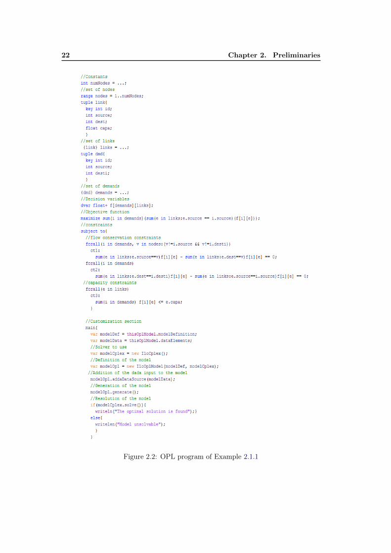
Example 2.1.1. Let G = (V,E) be a directed graph, where V is the set of nodes, Eis the set of edges and each edge (u, v) ∈ E has a capacity c(u, v) ≥ 0. Consider alsoa set D = {di = (si, ti), i = 1 . . . k} of k demands where si and ti are respectively thedemand source and destination. The objective of this MCF is to find the flows thatmaximize the network throughput while satisfying the capacity constraints. Thisproblem is modeled as follows:
LP
Maximize∑i=1...k
∑w∈V
fi(si, w)
subject to:∑v∈V
fi(u, v) =∑w∈V
fi(w, u) ∀ u ∈ V − {si, ti},∀ i = 1 . . . k∑w∈V
fi(w, ti) =∑v∈V
fi(si, v) ∀ i = 1 . . . k∑i=1...k
fi(u, v) ≤ c(u, v) ∀ (u, v) ∈ E
fi(u, v) ≥ 0 ∀ (u, v) ∈ E, ∀ i = 1 . . . k
The first two constraints are usually referred to as flow conservation constraintswhile the last constraint represents the capacity constraints. We talk about IntegerLinear Program (ILP) when all variables are integral and about Mixed Integer LinearProgram (MILP) when only some of the variables have to be integral.
One important property of linear programming is the notion of duality. To anylinear program of the form presented in Model (2.1), called primal, is associatedanother linear program, called dual of the following form:
min bT y
s.t. AT y ≥ c
y ∈ R+m (2.2)
2.2. Column generation 15
with the same vectors c and b and the same matrix A. y = (y1, y2, . . . , ym) is thevector of the dual variables where each variable yi is associated to the ith constraintof the primal model. Notice that the dual of the dual is the primal and that when theprimal has n variables andm constraints, its dual hasm variables and n constraints.Let x and y be feasible solutions of respectively the primal and the dual. Then:
bT y = yT b ≥ yT (Ax) = (yTA)x = (AT y)x ≥ cx (2.3)
This relation between the primal and the dual, called the weak duality theorem ,shows that the objective value of any feasible solution of a dual is an upper boundof the any feasible solution of the primal and consequently an upper bound of theoptimal solution of the primal. This is useful for estimating the gap between afeasible solution and the optimum when feasible solutions are available but findingthe optimal one is too hard.Furthermore, it has been proved through the strong duality theorem , that if theprimal has an optimal solution x∗, then the optimal solution y∗ of the dual is suchthat
cTx∗ = bT y∗
This relation is very important when solving some LP models. In Chapter 3 ofthis thesis, we use the dual values to express the reduced cost of variables, when ap-plying the column generation method presented in the next section. When dealingwith robust optimization method in Chapters 4 and 5, we use the strong duality the-orem. This allows us to express our optimization problem in a compact formulationthat is easier to solve than the original primal model.
2.2 Column generation
Column generation refers to linear programming (LP) algorithms designed to solvelarge-scale problems in which there are a huge number of variables compared to thenumber of constraints. In general, these linear programs are too large to considerall the variables explicitly. It is known that only a tiny fraction of the variables isneeded to prove optimality. So the goal of column generation is to find the optimalsolution of the problem without enumerating all variables, but by generating onlythe variables which have the potential to improve the objective function. To achievethat, the problem to be solved (the master problem, MP) is split into two sub-problems: the restricted master problem (RMP) and the pricing problem (PP).
Let us consider the MP of the form of the Model (2.1) and let J ′ ⊆ J be asubset of indices in J . The RMP is the master problem in which we consider onlythe variables with indices in J ′. Notice that when all the variables needed to findthe optimal solution of the MP will be generated and available in the RMP, then theRMP optimal solution will be the MP optimal solution. The PP is a new problemcreated to generate the variables that can improve the MP objective function. Thecolumn generation algorithm consists in solving iteratively the RMP followed by
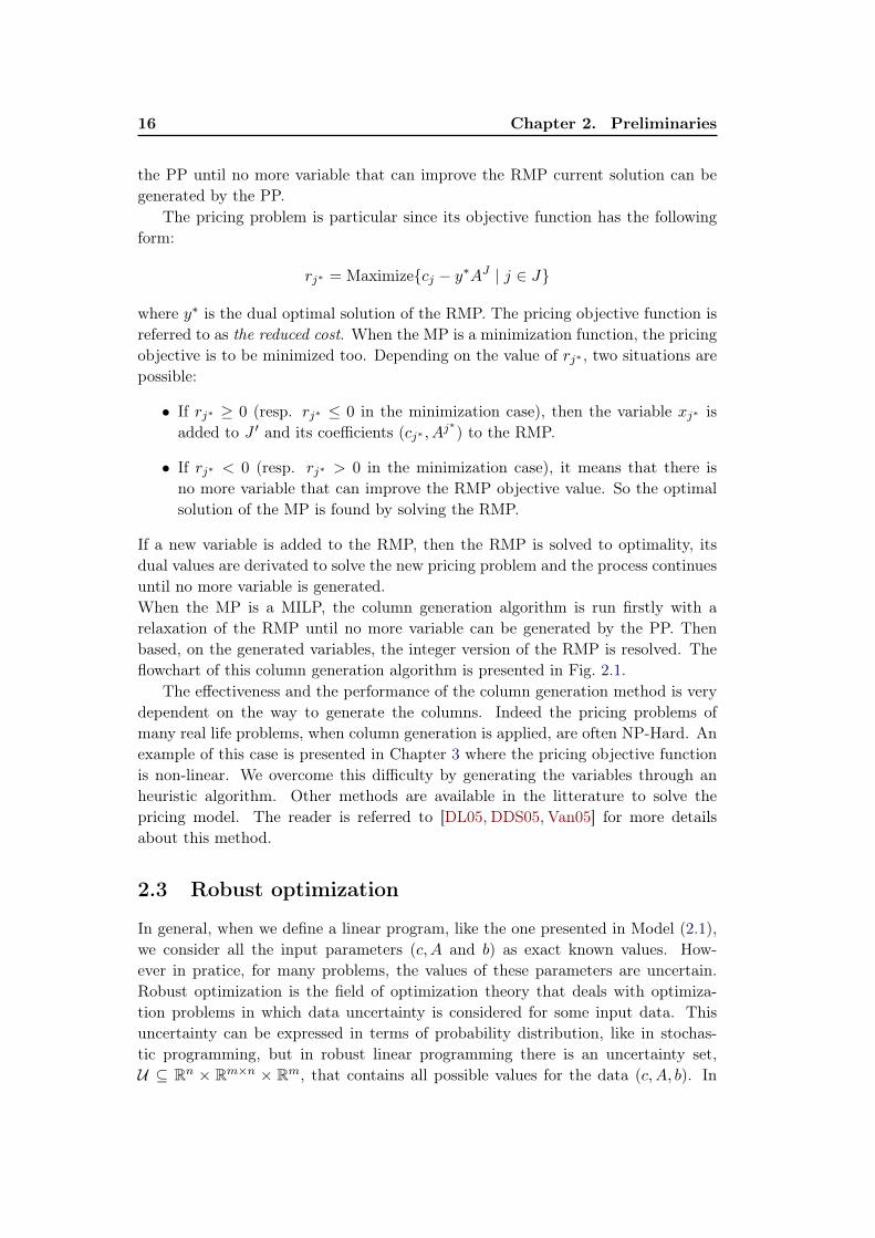
16 Chapter 2. Preliminaries
the PP until no more variable that can improve the RMP current solution can begenerated by the PP.
The pricing problem is particular since its objective function has the followingform:
rj∗ = Maximize{cj − y∗AJ | j ∈ J}
where y∗ is the dual optimal solution of the RMP. The pricing objective function isreferred to as the reduced cost. When the MP is a minimization function, the pricingobjective is to be minimized too. Depending on the value of rj∗ , two situations arepossible:
• If rj∗ ≥ 0 (resp. rj∗ ≤ 0 in the minimization case), then the variable xj∗ isadded to J ′ and its coefficients (cj∗ , Aj
∗) to the RMP.
• If rj∗ < 0 (resp. rj∗ > 0 in the minimization case), it means that there isno more variable that can improve the RMP objective value. So the optimalsolution of the MP is found by solving the RMP.
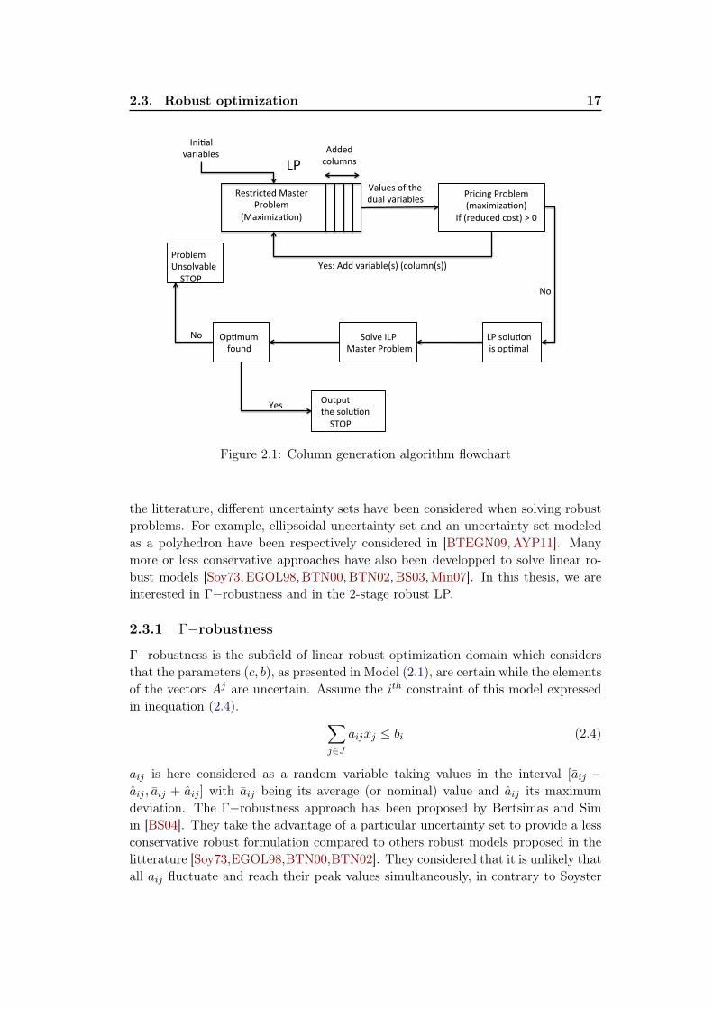
If a new variable is added to the RMP, then the RMP is solved to optimality, itsdual values are derivated to solve the new pricing problem and the process continuesuntil no more variable is generated.When the MP is a MILP, the column generation algorithm is run firstly with arelaxation of the RMP until no more variable can be generated by the PP. Thenbased, on the generated variables, the integer version of the RMP is resolved. Theflowchart of this column generation algorithm is presented in Fig. 2.1.
The effectiveness and the performance of the column generation method is verydependent on the way to generate the columns. Indeed the pricing problems ofmany real life problems, when column generation is applied, are often NP-Hard. Anexample of this case is presented in Chapter 3 where the pricing objective functionis non-linear. We overcome this difficulty by generating the variables through anheuristic algorithm. Other methods are available in the litterature to solve thepricing model. The reader is referred to [DL05, DDS05, Van05] for more detailsabout this method.
2.3 Robust optimization
In general, when we define a linear program, like the one presented in Model (2.1),we consider all the input parameters (c, A and b) as exact known values. How-ever in pratice, for many problems, the values of these parameters are uncertain.Robust optimization is the field of optimization theory that deals with optimiza-tion problems in which data uncertainty is considered for some input data. Thisuncertainty can be expressed in terms of probability distribution, like in stochas-tic programming, but in robust linear programming there is an uncertainty set,U ⊆ Rn × Rm×n × Rm, that contains all possible values for the data (c, A, b). In
2.3. Robust optimization 17
Restricted Master Problem
(Maximiza4on)
Added columns LP
Ini4al variables
Pricing Problem (maximiza4on)
If (reduced cost) > 0
Values of the dual variables
Yes: Add variable(s) (column(s))
LP solu4on is op4mal
Solve ILP Master Problem
Op4mum found
Output the solu4on STOP
Yes
No
Problem Unsolvable STOP
No
Figure 2.1: Column generation algorithm flowchart
the litterature, different uncertainty sets have been considered when solving robustproblems. For example, ellipsoidal uncertainty set and an uncertainty set modeledas a polyhedron have been respectively considered in [BTEGN09, AYP11]. Manymore or less conservative approaches have also been developped to solve linear ro-bust models [Soy73,EGOL98,BTN00,BTN02,BS03,Min07]. In this thesis, we areinterested in Γ−robustness and in the 2-stage robust LP.
2.3.1 Γ−robustness
Γ−robustness is the subfield of linear robust optimization domain which considersthat the parameters (c, b), as presented in Model (2.1), are certain while the elementsof the vectors Aj are uncertain. Assume the ith constraint of this model expressedin inequation (2.4). ∑
j∈Jaijxj ≤ bi (2.4)
aij is here considered as a random variable taking values in the interval [aij −aij , aij + aij ] with aij being its average (or nominal) value and aij its maximumdeviation. The Γ−robustness approach has been proposed by Bertsimas and Simin [BS04]. They take the advantage of a particular uncertainty set to provide a lessconservative robust formulation compared to others robust models proposed in thelitterature [Soy73,EGOL98,BTN00,BTN02]. They considered that it is unlikely thatall aij fluctuate and reach their peak values simultaneously, in contrary to Soyster
18 Chapter 2. Preliminaries
in [Soy73] that considered the same uncertain interval but proposed a model forthe case where all aij have a value equal to aij + aij . For that, they defined a realparameter 0 ≤ Γ ≤ |J | that represents the robustness level considered. Thus theΓ-robust solution stays optimal for all the cases where up to Γ of the uncertaincoefficients are allowed to change. For the sake of simplicity, we consider here Γ asan integer value. The objective of Γ−robustness is to find the optimal solution x
when Γ many (but arbitrary) coefficients deviate from their nominal values. Underthis assumption, Constraint (2.4) is replaced by:∑
j∈Jaijxj + max
{S|S⊆J ,|S|=Γ}
∑j∈S
aijxj ≤ bi (2.5)
where δ(x,Γ) = max{S|S⊆J ,|S|=Γ}∑
j∈S aijxj is the maximum deviation that can beintroduced in the constraint by at most Γ coefficients fluctuating simultaneously.Moreover, it has been proved by Bertsimas and Sim that given an arbitrary reali-sation, the probability that constraint (2.5) is violated is about 1− Φ(Γ−1√
p ), whereΦ is the cumulative distribution function of a standard normal and p is the numberof uncertain coefficients. With this model of uncertainty, Bertsimas and Sim showthat finding an optimal Γ−robust solution can be reduced to solving an ordinarylinear program only moderately increased in size, thus opening the way to largescale applications.
Γ−robustness is used in Chapters 4 and 5 of this thesis to model some traf-fic uncertainty considered in our problems. With this technique, we were ableto formulate the robust counterpart of the studied problems as linear programs.This method, applied in multiple network optimization problems in the littera-ture [KKR11, CKPT13, CKS13], has the main advantage to offer a good trade-offbetween the level of robustness and the cost of the solution. However this formula-tion is not satisfying when the uncertainty is on the Right-hand-side (RHS) of the LP.Indeed, when the objective is uncertain, Γ−robustness can be applied by transform-ing the objective into a constraint. Therefore, Minoux proposes a method to handlethis RHS uncertainty that is more natural in certain situations [Min07,Min11]. Wepresent it in the next section.
2.3.2 2-stage Robust LP with RHS uncertainty
RHS uncertainty in LP is a particular subclass of columnwise uncertainty model,unlike the "rowwise" when coefficents of a row are uncertain (Γ−robustness case).A first natural idea to handle such problems is to use the LP duality to reformulatethem as robust LPs with uncertainty on the objective. Minoux [Min07] shows inthis restrictive case that the objective of the robust counterpart of a dual problemis totally different from the one of the dual of a robust model. So one can not usestandard duality theory to convert a columnwise uncertain linear program into arowwise uncertain linear program while preserving equivalence.Also, Minoux proposed a model to handle the 2-stage robust LP problem with RHSuncertainty [Min11]. They are problems or applications in which the process of
2.4. Introduction to the Optimization Programming Language, OPL 19
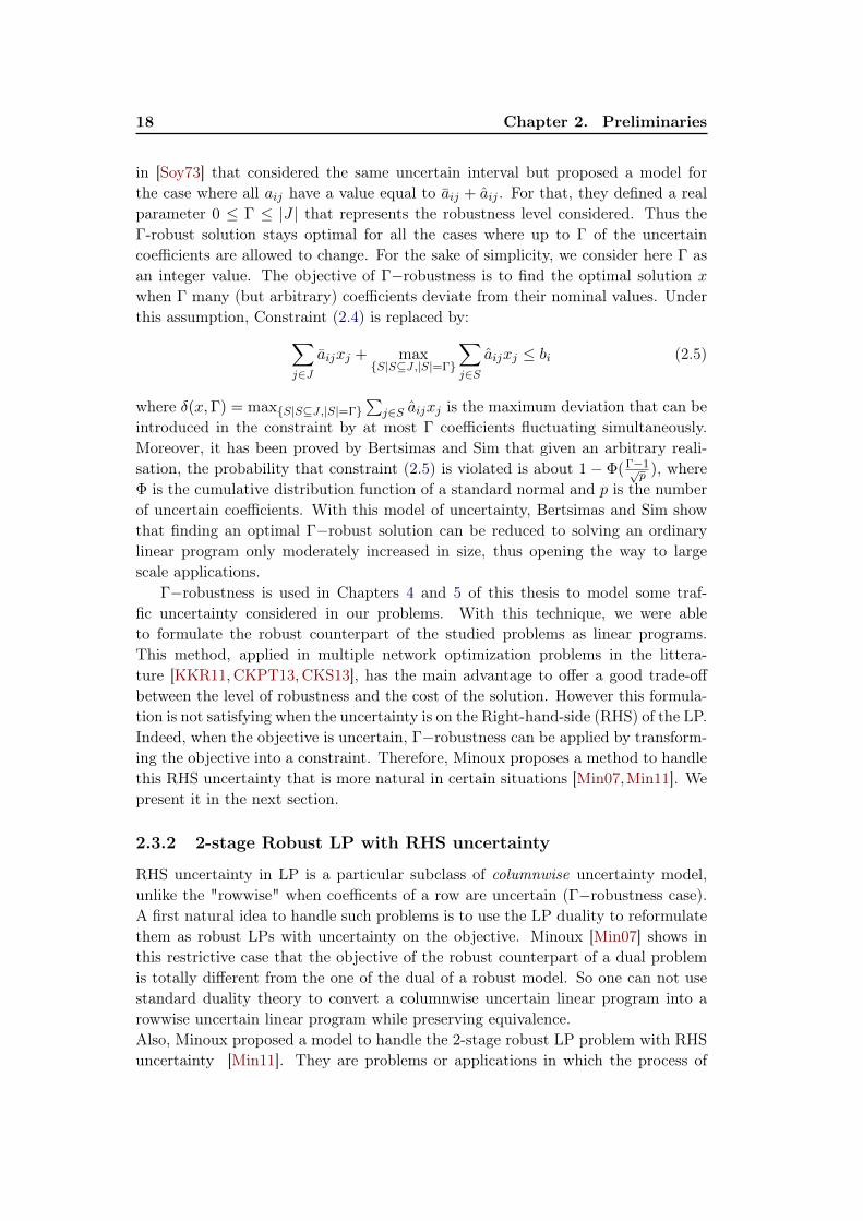
decision-making under uncertainty can be decomposed in two successive steps. Thefirst stage concerns the decisions to be made before knowing anything about whichrealization of uncertainty will arise while the second stage is related to the decisontaken after realization of uncertainty. The choice of this models was made becausethey can produce less conservative solutions as compared with single-stage robustLP models with RHS uncertainty. Model (2.6) represents the general form of theseproblems.
max cT y
s.t. A1y +A2z ≤ b
y, z ≥ 0(2.6)
with b taking value in the uncertainty set B. y and z are respectively the first andsecond stage variables. y is a feasible solution for the robust model when it belongsto the set Y = {y|y ≥ 0 and ∀ b ∈ B,∃ z ≥ 0 : A2z ≤ b − A1y} and the optimalsolution corresponds to
maxy∈Y
cT y
Based on Farka’s Lemma [DJ14], the author derives a large scale LP model forthe robust model. However a direct resolution of this model can be very difficultdue to its tremendeous number of constraints. A proposed way to overcome thisdifficulty is to apply the constraint generation method using a specific nonconvexseparation problem. It has been proved that these problems are generally NP-Hardbut polynomial algorithms can be found for some applications.
This method has been applyied to the cognitive network problem studied in theAppendix of this thesis. We detail there the methodology to obtain the large scaleLP of the robust model and also to define the specific separation problem adaptedto our application.
2.4 Introduction to the Optimization Programming Lan-guage, OPL
Once an optimization problem is modeled as a linear program, it remains to use itfor solving different problems instances. It is also important to compare the per-formances of the proposed model with other formulations, if any. This is useful foridentifying the advantages and the drawbacks of the formulation and eventually pro-pose improvements. To do so, we use various programming languages to implement(and solve) the mathematical model using some optimization solvers.
In the context of this thesis, different programming language have been used,depending on the model complexity: Python, Java and Optimization ProgrammingLanguage (OPL). Python and Java are well-known programming languages so we
20 Chapter 2. Preliminaries
will not present them here. OPL1 is a high-level optimization language currentlydevelopped by IBM to ease mathematical programming. For instance, it facilitatesthe implementation and test of linear programs using column generations. In thefollowing, we give a brief overview of the OPL language.
OPL, is a modeling language for mathematical programming and combinatorialoptimization problems modeled using LP, ILP, MILP or Constraint Programming(CP). It has originally been developped by Pascal van Hentenryck. Like othersmodeling languages such as AMPL [FGK93] and GAMS [BM04], OPL allows theuser to code mathematical models with a syntax similar to their algebraic notation.This allows for a very concise and readable definition of problems in the domain ofoptimization. Among its features, it proposes some new concepts for scheduling andresource allocation problems. It also allows to import data from databases or Excelspreasheets.
An OPL program consists of three (3) main sections:
1. Declaration of the constants and decision variables. This section is concernedwith the elements that compose the model. For each input of the problem,the user specifies its type and its value. OPL supports 2 data types, the basicones (integer, float, string, boolean) and the data collections (set, tuple, array,range). These constants can be initialized directly in the model file (.mod)or in a specific data file (.dat). Initializing the data in a separate file has theadvantage that it can be different for various problem instances. Concerningthe problem variables, the user defines their types and the domain of theirvalues. The decision variables are declared using the keyword dvar. Strictlypositive variables are declared using one of the data types int+ and float+.However variables in OPL can be of different types such as arrays.
2. Expression of the optimization model (objective function and constraints).The maximization or minimization objective is described and the user ex-presses the constraints that must be fulfilled for a solution to be feasible. Themodel is specified usingmaximize ... subject to.Though when no optimization is need, the set of constraints is specified usingthe keyword solve.
3. Customization of the search procedure or the solving algorithm. This sectionis dedicated to the expression of the searching method. This is the place wherethe user can implement a specific algorithm that uses the model variables andthat is needed to solve the problem. It is also the place where the model isgenerated and given to the solver for searching the solutions.
OPL allows multiple operations on the data. For instance, classical operationssuch as addition and multiplication are available on floats and integers. Other
1Although this section ressembles an advertisement for a commercial tool, this is not our ob-jective. The objective of this section is only to share a user experience on a tool that allowed usto implement quite easily complex formulations.
2.4. Introduction to the Optimization Programming Language, OPL 21
operations like getting the maximum or the minimum value of a set or rounding afloat are also possible. A complete list of available operations on data using OPLis referenced in [VH99] and also available online. Fig. 2.2 shows how to write theproblem of Example 2.1.1 using OPL.
As explained before, OPL is a modeling language that helps to express theconstraints on decision variables. However, an optimization application might alsoneed functionality for manipulating data. This “non-modeling” expressiveness of theOPL language is called scripting and available as OPL Script. It interacts with OPLmodels and helps to combine them. For instance, the customization of the searchprocedure is done using OPL Script. It manipulates scripting variables denotedby means of the keyword var. Note that these variables are different from OPLmodeling decision variables. OPL Script is used in three different situations:
• Preprocessing: to prepare the data that will be used by the model.
• Postprocessing: to work on or to manipulate model solutions
• Flow control: to define combinations of the data and the model and to solvethe model. It is also used to chain multiple models like in the case of columgeneration.
The development and the deployment of optimization problems modeled usingOPL are simplified when using the IBM ILOG CPLEX Optimization Studio [II14].This software package combines the solver engines such as IBM CPLEX and IBMCP Optimizer [II14] with a tightly integrated IDE and the modeling language OPL.With IBM academic Initiative, researchers and students can have a free acces toIBM ILOG CPLEX Optimization studio and CPLEX solvers. All documentationabout this language are available online. To get help when using this language, IBMteams and OPL users are reachable for technical discussions on the IBM forum.
22 Chapter 2. Preliminaries
Figure 2.2: OPL program of Example 2.1.1
Chapter 3
Dimensioning of MicrowaveWireless Networks
Contents3.1 Introduction . . . . . . . . . . . . . . . . . . . . . . . . . . . . 24
3.2 Related Work . . . . . . . . . . . . . . . . . . . . . . . . . . . . 25
3.2.1 Literature Review . . . . . . . . . . . . . . . . . . . . . . . . 25
3.2.2 Budget Constrained Optimization Model . . . . . . . . . . . 25
3.3 Network Model . . . . . . . . . . . . . . . . . . . . . . . . . . . 27
3.3.1 Definitions and Assumptions . . . . . . . . . . . . . . . . . . 28
3.3.2 Problem formulation . . . . . . . . . . . . . . . . . . . . . . . 28
3.3.3 An Illustrative Example . . . . . . . . . . . . . . . . . . . . . 30
3.4 Solution of the Model . . . . . . . . . . . . . . . . . . . . . . . 31
3.4.1 The Random Column Enumeration (RCE) heuristic . . . . . 34
3.4.2 The Modified Column Generation (MCG) heuristic . . . . . . 35
3.4.3 Initial Solution of the RMP . . . . . . . . . . . . . . . . . . . 36
3.5 Numerical Results . . . . . . . . . . . . . . . . . . . . . . . . . 37
3.5.1 Resolution process . . . . . . . . . . . . . . . . . . . . . . . . 38
3.5.2 Solution quality . . . . . . . . . . . . . . . . . . . . . . . . . . 38
3.5.3 Validation of the Results: Comparison with those of [CKCN14] 40
3.6 Conclusion . . . . . . . . . . . . . . . . . . . . . . . . . . . . . 40
We aim at dimensioning fixed broadband microwave wireless networks underunreliable channel conditions. As the capacity of microwave links is prone to vari-ations, such a dimensioning differs from the classical ones. Considering that linkcapacities of these networks vary depending on channel conditions, this problem canbe formulated as the determination of the minimum cost bandwidth assignment onthe links of the network in which the traffic requirements can be met with highprobability.
This problem was previously studied in [CKCN14]. The optimization modelproposed here represents a major step forward since we consider dynamic rout-ing. Experimental results show that the obtained solutions can save up to 45% ofbandwidth cost compared to the case where a bandwidth over-provisioning policy isapplied uniformly over all the links. Comparisons with previous work also show that
24 Chapter 3. Dimensioning of Microwave Wireless Networks
we can solve much larger instances than before in significantly shorter computingtimes, with a comparable reliability level.
3.1 Introduction
Offering a good quality service in telecommunications requires first of all a precisedesign and dimensioning of the network. The dimensioning consists in assigningsufficient ressources to networks to ensure in good conditions the routing of thetraffic. This step is much more crucial when designing microwave backauls to guar-antee a high network reliability. Actually, weather conditions and variability intime and in the space of the radio propagation channel introduce data transmissionoutage events. A common solution applied by network operators is the capacityover-provisioning of their networks.
In microwave networks, a link’s capacity is determined using the channel band-width and the modulation scheme used to transmit the traffic. However, the radiospectrum is a limited and expensive natural ressource whose efficient use is proned byregulatory authorithies. Thus, capacity overprovisioning is not cost effective for net-work operators, especially when extending their network coverage in remote areas.This is the reason that motivated us to study the minimum cost dimensioning prob-lem of microwave networks. We aim at assigning to each network link the minimumcost bandwidth that allow the routing of all traffic demands with high probability.This problem entails a complex design decision aiming at balancing bandwidth-costefficiency and network reliability in order to cope with channel fluctuations.
To overcome outage events due to fading phenomena, modern microwave systemsemploy adaptive modulation and coding which has been proved to considerablyenhance link performance [GC97,GC98]. In practice, to keep the BER (Bit errorrate) performance, this technique entails the variability of the link’s capacity.
Fading phenomena are described in statistical terms and the probabilityof fades of a particular magnitude can be evaluated through analytical tech-niques [Bar72,Vig75,Cra96]. Coudert et al proposed in [CNR10] to identify a finiteset of efficient radio configurations , for which no configuration that presents bet-ter bandwidth efficiency for a lower SNR (signal to noise ratio) requirement exists.They had then associated a discrete probability distribution with these selected con-figurations, derived either from statistical studies or from fading models and powerbudget calculations.
Under the assumption of a discrete probability distribution is known for eachmicrowave link and bandwidth, we propose here an optimization model to dimensionfixed broadband wireless microwave networks under unreliable channel conditions.The model determines the minimum cost bandwidth assignment of the links in thenetwork such that a required reliability level of the solution is satisfied, i.e., the se-lection of bandwidth is made in order to reduce bandwidth costs while guaranteeingthat traffic requirements can be met with high probability. We assume dynamicrouting (i.e., routing decisions are made according to channel conditions) so as to
3.2. Related Work 25
reduce the bandwidth over-provisioning during network planning.The chapter is organized as follows. In Section 3.2, we discuss the recent related
studies on dimensioning microwave networks. The proposed dimensioning model ispresented in Section 3.3 together with the assumed bandwidth/modulation prob-ability distribution. We then devise a solution of the model in Section 3.4. It isbased on a decomposition technique in order to ensure a scalable solution scheme.Numerical results are described in Section 3.5 and conclusions are drawn in the lastsection.
3.2 Related Work
We first survey the recent work on the dimensioning of microwave networks (Sec-tion 3.2.1), and then summarize the very recent work of [CKCN14] that we will usein order to validate the newly proposed dimensioning model (Section 3.2.2).
3.2.1 Literature Review
Computing the probability that a subset of nodes in a probabilistic network is con-nected is a classical computationally difficult problem [Bal86], even for the casein which the subset of nodes is restricted to a single source-destination pair, viz.the two-terminal network reliability problem [BJ88]. To the best of our knowl-edge, [DBH+07] was the first work to investigate the reliability of fixed broadbandwireless networks. The authors, however, assumed very strong hypotheses (e.g.single source-destination flow, uncapacitated network, unqualified failures) and ap-plied currently available algorithms for the two-terminal network reliability problem.They only presented results for a network with 5 nodes and 7 links.
Recently, the problem of determining the minimum cost bandwidth assign-ment of a network while guaranteeing a reliability level of the solution was studiedin [CCKN11a, CCKN11b, CKCN14]. The authors proposed a chance-constrainedprogramming approach in which, if the optimal bandwidth assignment and routingof traffic demands are accomplished, the reliability criterion guarantees that networkflows remain feasible with high probability. Under the assumption that links sufferfades independently, they proposed reformulations to standard MILP models.
One important remark to be made with respect to these previous approachesis that they consider static routing. In fact, bandwidth assignment and routingdecisions take place in different time and, therefore, it is possible to save bandwidthutilization by adopting dynamic routing.
3.2.2 Budget Constrained Optimization Model
In [CKCN14], to overcome the resolution challenges of the model defined for theoriginal problem, the authors proposed as well an alternative budget constrainedformulation for which they present a reliability analysis based on different budget
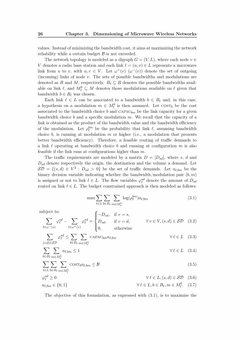
26 Chapter 3. Dimensioning of Microwave Wireless Networks
values. Instead of minimizing the bandwidth cost, it aims at maximizing the networkreliability while a certain budget B is not exceeded.
The network topology is modeled as a digraph G = (V,L), where each node v ∈V denotes a radio base station and each link ` = (u, v) ∈ L represents a microwavelink from u to v, with u, v ∈ V . Let ω+(v) (ω−(v)) denote the set of outgoing(incoming) links of node v. The sets of possible bandwidths and modulations aredenoted as B and M , respectively. B` ⊆ B denotes the possible bandwidths avail-able on link `, and M b
` ⊆ M denotes those modulations available on ` given thatbandwidth b ∈ B` was chosen.
Each link ` ∈ L can be associated to a bandwidth b ∈ B` and, in this case,a hypothesis on a modulation m ∈ M b
` is then assumed. Let costb be the costassociated to the bandwidth choice b and capacbm be the link capacity for a givenbandwidth choice b and a specific modulation m. We recall that the capacity of alink is obtained as the product of the bandwidth value and the bandwidth efficiencyof the modulation. Let ρbm` be the probability that link `, assuming bandwidthchoice b, is running at modulation m or higher (i.e., a modulation that presentsbetter bandwidth efficiency). Therefore, a feasible routing of traffic demands toa link ` operating at bandwidth choice b and running at configuration m is alsofeasible if the link runs at configurations higher than m.
The traffic requirements are modeled by a matrix D = [Dsd], where s, d andDsd denote respectively the origin, the destination and the volume a demand. LetSD = {(s, d) ∈ V 2 : Dsd > 0} be the set of traffic demands. Let a`,bm be thebinary decision variable indicating whether the bandwidth/modulation pair (b,m)
is assigned or not to link ` ∈ L. The flow variables ϕsd` denote the amount of Dsd
routed on link ` ∈ L. The budget constrained approach is then modeled as follows:
max∑`∈L
∑b∈B`
∑m∈Mb
`
log(ρbm` )a`,bm (3.1)
subject to:∑`∈ω−(v)
ϕsd` −∑
`∈ω+(v)
ϕsd` =
−Dsd, if v = s,Dsd, if v = d,0, otherwise
∀ v ∈ V, (s, d) ∈ SD (3.2)
∑(s,d)∈SD
ϕsd` ≤∑b∈B`
∑m∈Mb
`
capacbma`,bm ∀ ` ∈ L (3.3)
∑b∈B`
∑m∈Mb
`
a`,bm ≤ 1 ∀ ` ∈ L (3.4)
∑`∈L
∑b∈B`
∑m∈Mb
`
costba`,bm ≤ B (3.5)
ϕsd` ≥ 0 ∀ ` ∈ L, (s, d) ∈ SD (3.6)
a`,bm ∈ {0, 1} ∀ ` ∈ L, b ∈ B`,m ∈M b` . (3.7)
The objective of this formulation, as expressed with (3.1), is to maximize the
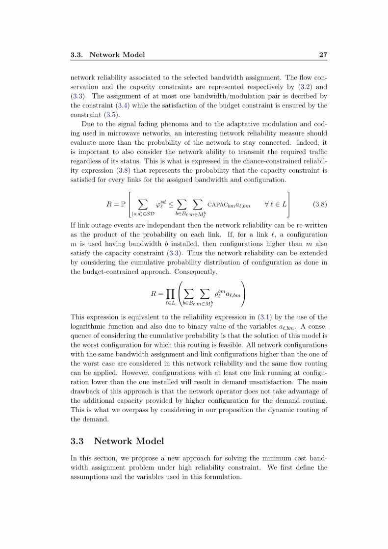
3.3. Network Model 27
network reliability associated to the selected bandwidth assignment. The flow con-servation and the capacity constraints are represented respectively by (3.2) and(3.3). The assignment of at most one bandwidth/modulation pair is decribed bythe constraint (3.4) while the satisfaction of the budget constraint is ensured by theconstraint (3.5).
Due to the signal fading phenoma and to the adaptative modulation and cod-ing used in microwave networks, an interesting network reliability measure shouldevaluate more than the probability of the network to stay connected. Indeed, itis important to also consider the network ability to transmit the required trafficregardless of its status. This is what is expressed in the chance-constrained reliabil-ity expression (3.8) that represents the probability that the capacity constraint issatisfied for every links for the assigned bandwidth and configuration.
R = P
∑(s,d)∈SD
ϕsd` ≤∑b∈B`
∑m∈Mb
`
capacbma`,bm ∀ ` ∈ L
(3.8)
If link outage events are independant then the network reliability can be re-writtenas the product of the probability on each link. If, for a link `, a configurationm is used having bandwidth b installed, then configurations higher than m alsosatisfy the capacity constraint (3.3). Thus the network reliability can be extendedby considering the cumulative probability distribution of configuration as done inthe budget-contrained approach. Consequently,
R =∏`∈L
∑b∈B`
∑m∈Mb
`
ρbm` a`,bm
This expression is equivalent to the reliability expression in (3.1) by the use of thelogarithmic function and also due to binary value of the variables a`,bm. A conse-quence of considering the cumulative probability is that the solution of this model isthe worst configuration for which this routing is feasible. All network configurationswith the same bandwidth assignment and link configurations higher than the one ofthe worst case are considered in this network reliability and the same flow routingcan be applied. However, configurations with at least one link running at configu-ration lower than the one installed will result in demand unsatisfaction. The maindrawback of this approach is that the network operator does not take advantage ofthe additional capacity provided by higher configuration for the demand routing.This is what we overpass by considering in our proposition the dynamic routing ofthe demand.
3.3 Network Model
In this section, we proprose a new approach for solving the minimum cost band-width assignment problem under high reliability constraint. We first define theassumptions and the variables used in this formulation.
28 Chapter 3. Dimensioning of Microwave Wireless Networks
3.3.1 Definitions and Assumptions
For the sake of clarity, our model is based on the same notations and definitionsrelated to network topology model, radio configurations and traffic demands, used inSection 3.2.2. Note however that we add hereM` ⊆M to denote all the modulationsavailable on link ` regardless on a particular bandwidth b, and the set BM` torepresent the bandwidth/modulation pairs available on `. Also, the definition of theprobability distribution associated to the pairs in BM` is slightly different. Insteadof using the cumulative probability distribution denoted by ρbm` above, we denoteby π`,bm the probability that exactly the modulation m is running on link ` havinginstalled the bandwidth b. Hence we have:
∑(b,m)∈BM`
π`,bm = 1 ∀` ∈ L,∀b ∈ B` (3.9)
We introduce in the following the notion of configuration which is defined as theset of links configurations in the network. In particular, a configuration c corre-sponds to a network dimensioning (i.e., bandwidth choice for each link) and, giventhe dimensioning, a radio configuration (i.e., modulation for each link). Formally,the binary parameters ac`,b and a
c`,m denote whether the link ` uses the bandwidth
b and the modulation m, respectively, within the configuration c. The parameterac`,bm is set to 1 for some link ` if the corresponding bandwidth and modulationparameters are also equal to 1. Naturally, only one bandwidth and one modulationcould be used by a link ` in a configuration c.
With the assumption of independence between the probability distribution ofeach link, the occurrence probability pc of a configuration c can be written as:
pc =∏`∈L
∑(b,m)∈BM`
π`,bm ac`,bm ∀c ∈ C (3.10)
where C represents the set of all possible configurations.Note that, in our model, it is possible that not all the traffic demands are com-
pletely satisfied by the configurations in C. Indeed, we define by the parameter δcsdthe amount of unsatisfied demand from source node s to destination node d, due tocapacity constraints of configuration c.
3.3.2 Problem formulation
Our objective is to assign the bandwidths on the links in L so that the total band-width renting cost is minimized but also the amount of unsatisfied demands. Asoutput of our solution, we will have a set of network configurations, all with theoptimal bandwidth assignment, that allow a dynamic routing of the traffic underradio propagation environment variation. The main variables of our model are:
• xc: set to 1 if the scenario c is considered, 0 otherwise
3.3. Network Model 29
• z`,b: set to 1 if bandwidth b is used on link ` in all the considered configurations,0 otherwise.
• z`: bandwidth cost of link `
Furthermore, we denote by the variable y`,bm the amount of unfeasibility withrespect to the discrete probability distribution of modulation for given link ` ∈ L and(b,m) ∈ BM`. An important point here is that we do not consider all the possibleconfigurations in our solution because many of them are very unlikely. Thus, if wedenote by C ′ the set of considered configurations (xc = 1, c ∈ C ′),
∑c∈C′
pc will be
strictly less than 1. So, the total probability that some link ` uses the configuration(b,m) in the solution does not necessarily match the given probability π`,bm. Here iswhere the variable y`,bm comes into play. Yet, we ensure that the solution providesa satisfactory grade of service to the network operator by enforcing that p =
∑c∈C′
pc
is at least some minimum value pmin, generally close to 1. In the sequel, we refer tothis probability sum p as the network reliability. So the configurations in C ′ coverthe scenarios that appear in the network p% of the time, and the model shouldensure a feasible routing for each of them.
Our optimization model can be stated as follows:
30 Chapter 3. Dimensioning of Microwave Wireless Networks
min∑`∈L
z` + penal1
∑(s,d)∈SD
∑c∈C
δcsdpc xc + penal2
∑`∈L
∑(b,m)∈BM`
y`,bm (3.11)
∑c∈C
pc xc ≥ pmin (3.12)∑c∈C
ac`,bm pc xc + y`,bm = z`,b π`,bm ∀ ` ∈ L,m ∈M`,
b ∈ B` : (b,m) ∈ BM` (3.13)∑b∈B`
z`,b = 1 ∀ ` ∈ L (3.14)
costb z`,b ≤ z` ∀ ` ∈ L, b ∈ B` (3.15)
z`,b ∈ {0, 1} ∀ ` ∈ L, b ∈ B` (3.16)
z` ≥ 0 ∀ ` ∈ L (3.17)
xc ∈ {0, 1} ∀ c ∈ C (3.18)
y`,bm ∈ [0, 1] ∀ ` ∈ L, (b,m) ∈ BM`. (3.19)
penal1 and penal2 are positive constants which penalize any amount of de-mand dissatisfaction and probability unfeasibility in the solution, respectively. Theprobability unfeasibility level of each link ` (y`,bm) is determined in constraint (3.13)according to the considered configurations (xc) and the assigned bandwidth b (z`,b).The constraint (3.15) determines the bandwidth cost value for a given link. Notethat the variables z` are not restricted in constraint(3.17) to be integers even if thecost values are always so: this will simplify the solution of the model.
The number of constraints of this problem is in the order of O(|L|× |BM|). Thisremains reasonable as the number of elements of BM is quite limited in practice.
3.3.3 An Illustrative Example
Consider a small microwave network with three links : `1, `2, `3. We use the followingbandwidth and modulation values:
• B = {b1 = 7MHz, b2 = 14MHz}
• M = {m1 = QPSK,m2 = 16QAM}
ThusBM = {(7MHz,QPSK), (7MHz, 16QAM), (14MHz,QPSK), (14MHz, 16QAM)}
The discrete probability distributions of the bandwidth/modulation pair of eachlink are given in Table 3.1. Note that the number of possible network configurationsin this example is 43 = 64. Table 3.2 shows only the network scenarios correspondingto the network dimensioning z`1,b1 = z`2,b1 = z`3,b1 = 1.
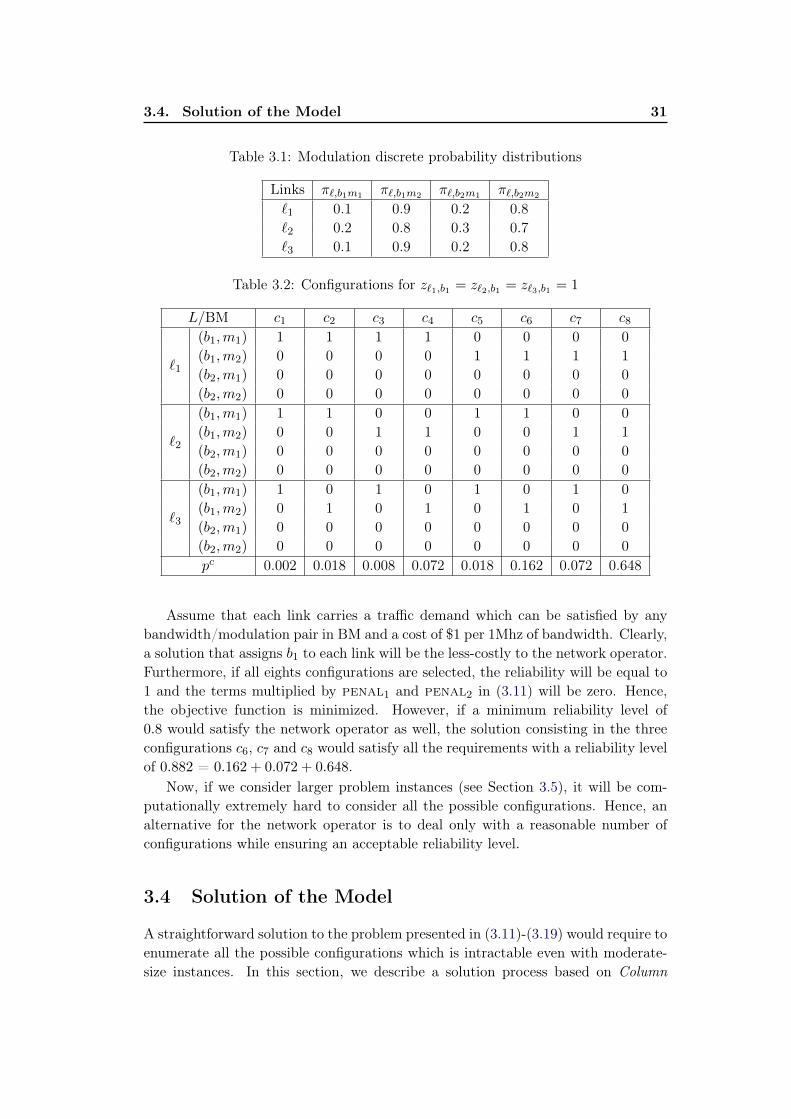
3.4. Solution of the Model 31
Table 3.1: Modulation discrete probability distributions
Links π`,b1m1 π`,b1m2 π`,b2m1 π`,b2m2
`1 0.1 0.9 0.2 0.8`2 0.2 0.8 0.3 0.7`3 0.1 0.9 0.2 0.8
Table 3.2: Configurations for z`1,b1 = z`2,b1 = z`3,b1 = 1
L/BM c1 c2 c3 c4 c5 c6 c7 c8
`1
(b1,m1) 1 1 1 1 0 0 0 0(b1,m2) 0 0 0 0 1 1 1 1(b2,m1) 0 0 0 0 0 0 0 0(b2,m2) 0 0 0 0 0 0 0 0
`2
(b1,m1) 1 1 0 0 1 1 0 0(b1,m2) 0 0 1 1 0 0 1 1(b2,m1) 0 0 0 0 0 0 0 0(b2,m2) 0 0 0 0 0 0 0 0
`3
(b1,m1) 1 0 1 0 1 0 1 0(b1,m2) 0 1 0 1 0 1 0 1(b2,m1) 0 0 0 0 0 0 0 0(b2,m2) 0 0 0 0 0 0 0 0pc 0.002 0.018 0.008 0.072 0.018 0.162 0.072 0.648
Assume that each link carries a traffic demand which can be satisfied by anybandwidth/modulation pair in BM and a cost of $1 per 1Mhz of bandwidth. Clearly,a solution that assigns b1 to each link will be the less-costly to the network operator.Furthermore, if all eights configurations are selected, the reliability will be equal to1 and the terms multiplied by penal1 and penal2 in (3.11) will be zero. Hence,the objective function is minimized. However, if a minimum reliability level of0.8 would satisfy the network operator as well, the solution consisting in the threeconfigurations c6, c7 and c8 would satisfy all the requirements with a reliability levelof 0.882 = 0.162 + 0.072 + 0.648.
Now, if we consider larger problem instances (see Section 3.5), it will be com-putationally extremely hard to consider all the possible configurations. Hence, analternative for the network operator is to deal only with a reasonable number ofconfigurations while ensuring an acceptable reliability level.
3.4 Solution of the Model
A straightforward solution to the problem presented in (3.11)-(3.19) would require toenumerate all the possible configurations which is intractable even with moderate-size instances. In this section, we describe a solution process based on Column
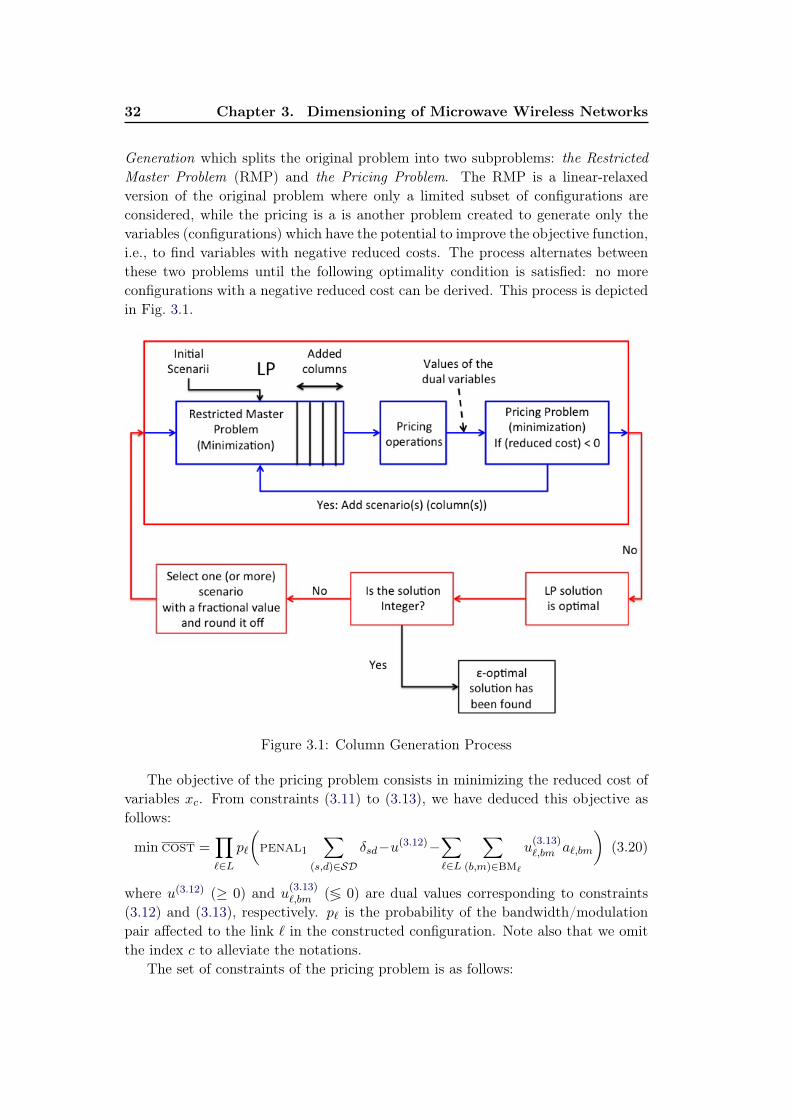
32 Chapter 3. Dimensioning of Microwave Wireless Networks
Generation which splits the original problem into two subproblems: the RestrictedMaster Problem (RMP) and the Pricing Problem. The RMP is a linear-relaxedversion of the original problem where only a limited subset of configurations areconsidered, while the pricing is a is another problem created to generate only thevariables (configurations) which have the potential to improve the objective function,i.e., to find variables with negative reduced costs. The process alternates betweenthese two problems until the following optimality condition is satisfied: no moreconfigurations with a negative reduced cost can be derived. This process is depictedin Fig. 3.1.
Figure 3.1: Column Generation Process
The objective of the pricing problem consists in minimizing the reduced cost ofvariables xc. From constraints (3.11) to (3.13), we have deduced this objective asfollows:
min cost =∏`∈L
p`
(penal1
∑(s,d)∈SD
δsd−u(3.12)−∑`∈L
∑(b,m)∈BM`
u(3.13)`,bm a`,bm
)(3.20)
where u(3.12) (≥ 0) and u(3.13)`,bm (≶ 0) are dual values corresponding to constraints
(3.12) and (3.13), respectively. p` is the probability of the bandwidth/modulationpair affected to the link ` in the constructed configuration. Note also that we omitthe index c to alleviate the notations.
The set of constraints of the pricing problem is as follows:
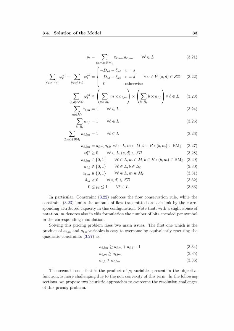
3.4. Solution of the Model 33
p` =∑
(b,m)∈BM`
π`,bm a`,bm ∀` ∈ L (3.21)
∑`∈ω−(v)
ϕsd` −∑
`∈ω+(v)
ϕsd` =
−Dsd + δsd v = s
Dsd − δsd v = d
0 otherwise
∀ v ∈ V, (s, d) ∈ SD (3.22)
∑(s,d)∈SD
ϕsd` ≤
∑m∈M`
m× a`,m
×∑b∈B`
b× a`,b
∀ ` ∈ L (3.23)
∑m∈M`
a`,m = 1 ∀` ∈ L (3.24)
∑b∈B`
a`,b = 1 ∀` ∈ L (3.25)
∑(b,m)∈BM`
a`,bm = 1 ∀` ∈ L (3.26)
a`,bm = a`,m a`,b ∀` ∈ L,m ∈M, b ∈ B : (b,m) ∈ BM` (3.27)
ϕsd` ≥ 0 ∀` ∈ L, (s, d) ∈ SD (3.28)
a`,bm ∈ {0, 1} ∀` ∈ L,m ∈M, b ∈ B : (b,m) ∈ BM` (3.29)
a`,b ∈ {0, 1} ∀` ∈ L, b ∈ B` (3.30)
a`,m ∈ {0, 1} ∀` ∈ L,m ∈M` (3.31)
δsd ≥ 0 ∀(s, d) ∈ SD (3.32)
0 ≤ p` ≤ 1 ∀` ∈ L (3.33)
In particular, Constraint (3.22) enforces the flow conservation rule, while theconstraint (3.23) limits the amount of flow transmitted on each link by the corre-sponding attributed capacity in this configuration. Note that, with a slight abuse ofnotation, m denotes also in this formulation the number of bits encoded per symbolin the corresponding modulation.
Solving this pricing problem rises two main issues. The first one which is theproduct of a`,m and a`,b variables is easy to overcome by equivalently rewriting thequadratic constraints (3.27) as:
a`,bm ≥ a`,m + a`,b − 1 (3.34)
a`,m ≥ a`,bm (3.35)
a`,b ≥ a`,bm (3.36)
The second issue, that is the product of p` variables present in the objectivefunction, is more challenging due to the non convexity of this term. In the followingsections, we propose two heuristic approaches to overcome the resolution challengesof this pricing problem.
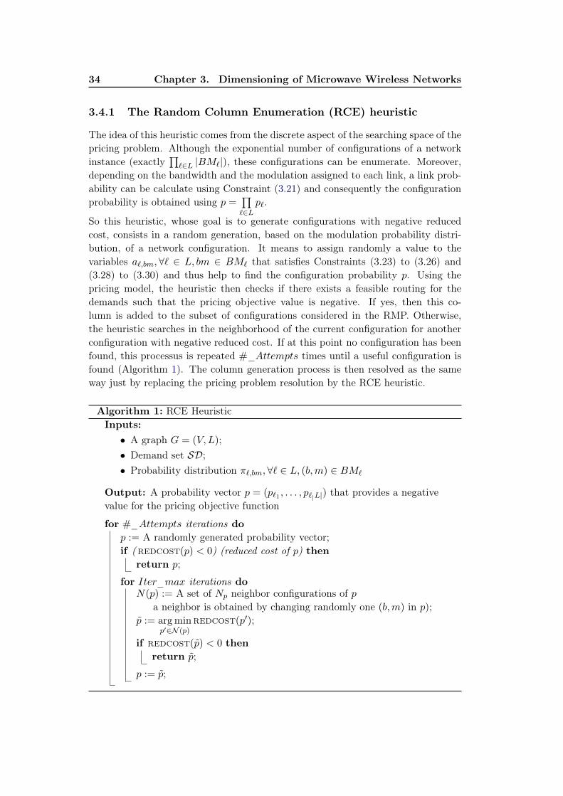
34 Chapter 3. Dimensioning of Microwave Wireless Networks
3.4.1 The Random Column Enumeration (RCE) heuristic
The idea of this heuristic comes from the discrete aspect of the searching space of thepricing problem. Although the exponential number of configurations of a networkinstance (exactly
∏`∈L |BM`|), these configurations can be enumerate. Moreover,
depending on the bandwidth and the modulation assigned to each link, a link prob-ability can be calculate using Constraint (3.21) and consequently the configurationprobability is obtained using p =
∏`∈L
p`.
So this heuristic, whose goal is to generate configurations with negative reducedcost, consists in a random generation, based on the modulation probability distri-bution, of a network configuration. It means to assign randomly a value to thevariables a`,bm,∀` ∈ L, bm ∈ BM` that satisfies Constraints (3.23) to (3.26) and(3.28) to (3.30) and thus help to find the configuration probability p. Using thepricing model, the heuristic then checks if there exists a feasible routing for thedemands such that the pricing objective value is negative. If yes, then this co-lumn is added to the subset of configurations considered in the RMP. Otherwise,the heuristic searches in the neighborhood of the current configuration for anotherconfiguration with negative reduced cost. If at this point no configuration has beenfound, this processus is repeated #_Attempts times until a useful configuration isfound (Algorithm 1). The column generation process is then resolved as the sameway just by replacing the pricing problem resolution by the RCE heuristic.
Algorithm 1: RCE HeuristicInputs:• A graph G = (V,L);• Demand set SD;• Probability distribution π`,bm, ∀` ∈ L, (b,m) ∈ BM`
Output: A probability vector p = (p`1 , . . . , p`|L|) that provides a negativevalue for the pricing objective function
for #_Attempts iterations dop := A randomly generated probability vector;if (redcost(p) < 0) (reduced cost of p) then
return p;
for Iter_max iterations doN(p) := A set of Np neighbor configurations of p
a neighbor is obtained by changing randomly one (b,m) in p);p := arg min
p′∈N (p)redcost(p′);
if redcost(p) < 0 thenreturn p;
p := p;
3.4. Solution of the Model 35
Though this heuristic has the hability to generate many configurations withnegative reduced cost for small size instances, applying it to larger size instances willnot be efficient due to the huge size of the search space. Indeed, the RCE heuristicsearches, at each iteration of the column generation process, for a configurationwith negative reduced cost in at most #_Attempts of different and randomly chosenneighborhoods. When no interesting configuration is found, the algorithm stops withthe assumption that no more useful configuration can be found. When the size ofthe search space is very large, this heuristic may miss many available configurationswith negative reduced cost at the time the algorithm ends. Hence we propose analternative method for generating the configurations that relies on a modified versionof the MILP pricing problem.
3.4.2 The Modified Column Generation (MCG) heuristic
To overcome the difficulty to solve the pricing problem because of the presence ofthe non convex term, we introduce here a slight transformation in this problem.As mentionned before, configurations generated by the pricing problem are onlythose for which the objective value of the pricing problem is negative. We knowthat the term
∏`∈L p` is always positive and thus will not affect the sign of the
pricing problem objective function. So the idea here is to generate the variables(configurations) using the same pricing problem from which the non-linear term ofthe objective is removed. In this way we are guaranteed to solve the pricing prob-lem while generating all useful configurations that can improve the RMP objectivefunction. Moreover, we consider only the configurations that satisfy all the trafficrequirements. After a new configuration c is found through this modified pricingmodel, we use a local search heuristic in order to generate other valid configurationsthat will also be added to the RMP. The aim of this heuristic is to speed up theresolution of the problem. These configurations are obtained from c by modifyingthe modulation of some randomly selected links of configuration c.
The resolution algorithm, (see Fig. 3.2), consists then in solving iteratively theRMP and the modified pricing problem until no more configuration with negativereduced cost can be find. This is followed by an ILP resolution of the RMP thatresults in a set of network configurations with a minimum bandwidth cost. Noticethat this algorithm, because of the use of the modified pricing problem is a heuristicmethod. In order to increase the solution reliability, we apply a post-optimizationprocedure.
It first chooses the configuration c1 that has the highest probability among thosethat were selected by the ILP resolution of the RMP. At this stage, the bandwidth ofeach link is already assigned. Then, we derive new configurations by modifying themodulation of some randomly chosen links of c1. Then using the modified pricingproblem, we verify the existence of a routing solution for these configurations. Ifit exists, then the new derivative configurations will be added to the RMP. Thiscontributes to increase the final solution reliability without changing the bandwidthassignment cost.
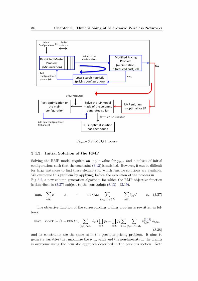
36 Chapter 3. Dimensioning of Microwave Wireless Networks
Added columns LP Ini0al
Configura0ons
Modified Pricing Problem
(minimiza0on) If (reduced cost) < 0
Values of the dual variables
No
Restricted Master Problem
(Minimiza0on)
Yes Local search heuris0c (pricing configura0on)
Add configura0on(s) (column(s))
RMP solu0on is op0mal for LP
Solve the ILP model made of the columns generated so far
Post-‐op0miza0on on the main
configura0on
1st ILP resolu0on
ILP ε-‐op0mal solu0on has been found
2nd ILP resolu0on
Add new configura0on(s) (column(s))
Figure 3.2: MCG Process
3.4.3 Initial Solution of the RMP
Solving the RMP model requires an input value for pmin and a subset of initialconfigurations such that the constraint (3.12) is satisfied. However, it can be difficultfor large instances to find these elements for which feasible solutions are available.We overcome this problem by applying, before the execution of the process inFig 3.2, a new column generation algorithm for which the RMP objective functionis described in (3.37) subject to the constraints (3.13) - (3.19).
max∑c∈C
pc xc − penal1
∑(vs,vd)∈SD
∑c∈C
δcsdpc xc (3.37)
The objective function of the corresponding pricing problem is rewritten as fol-lows:
max cost′ = (1− penal1
∑(s,d)∈SD
δsd)∏`∈L
p` −∏`∈L
p`∑`∈L
∑(b,m)∈BM`
u(3.13)`,bm a`,bm
(3.38)and its constraints are the same as in the previous pricing problem. It aims togenerate variables that maximize the pmin value and the non-linearity in the pricingis overcome using the heuristic approach described in the previous section. Note
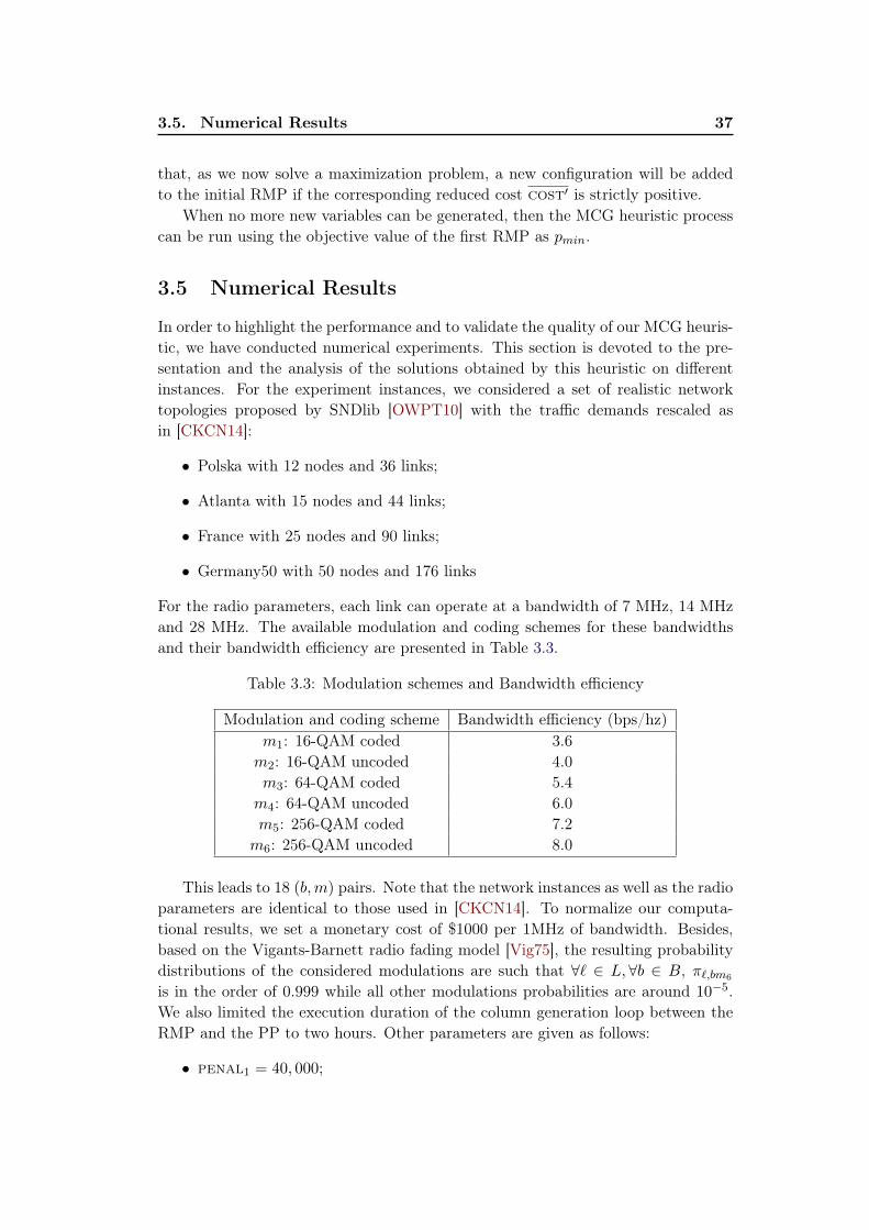
3.5. Numerical Results 37
that, as we now solve a maximization problem, a new configuration will be addedto the initial RMP if the corresponding reduced cost cost′ is strictly positive.
When no more new variables can be generated, then the MCG heuristic processcan be run using the objective value of the first RMP as pmin.
3.5 Numerical Results
In order to highlight the performance and to validate the quality of our MCG heuris-tic, we have conducted numerical experiments. This section is devoted to the pre-sentation and the analysis of the solutions obtained by this heuristic on differentinstances. For the experiment instances, we considered a set of realistic networktopologies proposed by SNDlib [OWPT10] with the traffic demands rescaled asin [CKCN14]:
• Polska with 12 nodes and 36 links;
• Atlanta with 15 nodes and 44 links;
• France with 25 nodes and 90 links;
• Germany50 with 50 nodes and 176 links
For the radio parameters, each link can operate at a bandwidth of 7 MHz, 14 MHzand 28 MHz. The available modulation and coding schemes for these bandwidthsand their bandwidth efficiency are presented in Table 3.3.
Table 3.3: Modulation schemes and Bandwidth efficiency
Modulation and coding scheme Bandwidth efficiency (bps/hz)m1: 16-QAM coded 3.6m2: 16-QAM uncoded 4.0m3: 64-QAM coded 5.4m4: 64-QAM uncoded 6.0m5: 256-QAM coded 7.2m6: 256-QAM uncoded 8.0
This leads to 18 (b,m) pairs. Note that the network instances as well as the radioparameters are identical to those used in [CKCN14]. To normalize our computa-tional results, we set a monetary cost of $1000 per 1MHz of bandwidth. Besides,based on the Vigants-Barnett radio fading model [Vig75], the resulting probabilitydistributions of the considered modulations are such that ∀` ∈ L,∀b ∈ B, π`,bm6
is in the order of 0.999 while all other modulations probabilities are around 10−5.We also limited the execution duration of the column generation loop between theRMP and the PP to two hours. Other parameters are given as follows:
• penal1 = 40, 000;

38 Chapter 3. Dimensioning of Microwave Wireless Networks
• penal2 = 50;
• pmin = 0.9.
3.5.1 Resolution process
The high variability of the probability distributions described above and the in-dependence between link probabilities produce a tremendous number of possibleconfigurations with very low probability value. In order to prevent generating suchmeaningless configurations, e.g., with probability in order of 10−75, we add thefollowing constraint to the modified pricing problem.
p` ≥ 0.1 ` ∈ L (3.39)
Table 3.4: CG Results
Polska Atlanta France Germany50# Generated conf. 606 635 629 454
# Used conf. 78 16 102 17
Table 3.4 shows that the number of total configurations generated by our res-olution process represents only a very tiny fraction of the number of possible con-figurations, which is
∏`∈L |BM`|. That means that our process focus primarily on
the most significant configurations in terms of probability and demand satisfaction.Also, we can observe that the best solutions in terms of cost will consider onlya limited number of configurations while reaching the desired reliability level, asdescribed below. Note that all the generated configurations satisfy the totality oftraffic demands, i.e., δsd = 0,∀(s, d) ∈ SD. This gives additional strength to ourdefinition of the network reliability since our solution now covers very high per-centage of the most frequent configurations while ensuring satisfaction of all trafficrequirement.
3.5.2 Solution quality
We highlight here the quality of the solutions obtained by our MCGmethod. Fig. 3.3shows, for each network topology, the cost saving that can be achieved by thenetwork operator compared to the worst case where the highest cost bandwidth isinstalled on every links. The results expose a significant cost saving ranging from33% to 45%, while achieving a high reliability level. As the saving increases with thenetwork size, one would also notice some decrease in the reliability. This is due inpart to Constraint (3.39) but mostly to the fact that it is much harder to maintainthe same reliability level because the configuration probabilities would decrease byan order of magnitude by just adding one link to the network.
The quality of our method can also be evaluated through the reliability gapsbetween our solutions and the worst case, as shown in Fig. 3.4. We can see that the
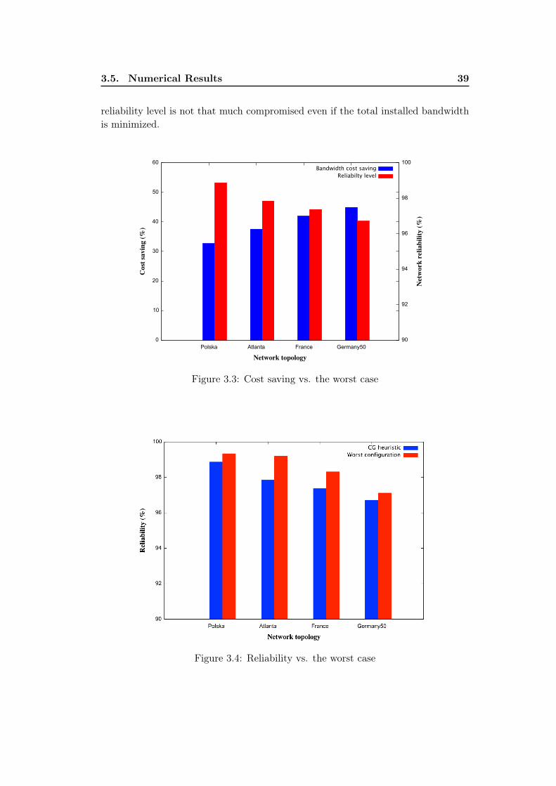
3.5. Numerical Results 39
reliability level is not that much compromised even if the total installed bandwidthis minimized.
Figure 3.3: Cost saving vs. the worst case
Figure 3.4: Reliability vs. the worst case
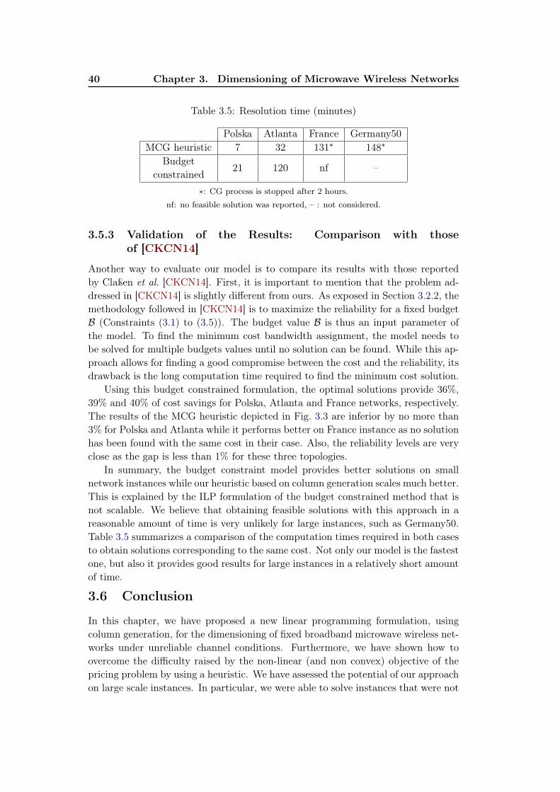
40 Chapter 3. Dimensioning of Microwave Wireless Networks
Table 3.5: Resolution time (minutes)
Polska Atlanta France Germany50MCG heuristic 7 32 131∗ 148∗
Budget21 120 nf –
constrained∗: CG process is stopped after 2 hours.
nf: no feasible solution was reported, – : not considered.
3.5.3 Validation of the Results: Comparison with thoseof [CKCN14]
Another way to evaluate our model is to compare its results with those reportedby Claßen et al. [CKCN14]. First, it is important to mention that the problem ad-dressed in [CKCN14] is slightly different from ours. As exposed in Section 3.2.2, themethodology followed in [CKCN14] is to maximize the reliability for a fixed budgetB (Constraints (3.1) to (3.5)). The budget value B is thus an input parameter ofthe model. To find the minimum cost bandwidth assignment, the model needs tobe solved for multiple budgets values until no solution can be found. While this ap-proach allows for finding a good compromise between the cost and the reliability, itsdrawback is the long computation time required to find the minimum cost solution.
Using this budget constrained formulation, the optimal solutions provide 36%,39% and 40% of cost savings for Polska, Atlanta and France networks, respectively.The results of the MCG heuristic depicted in Fig. 3.3 are inferior by no more than3% for Polska and Atlanta while it performs better on France instance as no solutionhas been found with the same cost in their case. Also, the reliability levels are veryclose as the gap is less than 1% for these three topologies.
In summary, the budget constraint model provides better solutions on smallnetwork instances while our heuristic based on column generation scales much better.This is explained by the ILP formulation of the budget constrained method that isnot scalable. We believe that obtaining feasible solutions with this approach in areasonable amount of time is very unlikely for large instances, such as Germany50.Table 3.5 summarizes a comparison of the computation times required in both casesto obtain solutions corresponding to the same cost. Not only our model is the fastestone, but also it provides good results for large instances in a relatively short amountof time.
3.6 Conclusion
In this chapter, we have proposed a new linear programming formulation, usingcolumn generation, for the dimensioning of fixed broadband microwave wireless net-works under unreliable channel conditions. Furthermore, we have shown how toovercome the difficulty raised by the non-linear (and non convex) objective of thepricing problem by using a heuristic. We have assessed the potential of our approachon large scale instances. In particular, we were able to solve instances that were not

3.6. Conclusion 41
reachable by other methods.As future work, we plan to improve the heuristic used to solve the pricing problem
in order to increase the reliability of the solutions, and eventually find solutions withsmaller cost. We would also like to propose a fixed budget formulation in order tobuild the Pareto front of the solution space. Moreover, we will investigate on thecorrelations of the links fades that are due to environmental (weather) conditions.

Chapter 4
Infrastructure sharing
Contents4.1 Introduction . . . . . . . . . . . . . . . . . . . . . . . . . . . . 43
4.2 Problem definition and nominal formulation . . . . . . . . . 46
4.2.1 Problem situation . . . . . . . . . . . . . . . . . . . . . . . . 46
4.2.2 Static model formulation . . . . . . . . . . . . . . . . . . . . 46
4.3 Robust model . . . . . . . . . . . . . . . . . . . . . . . . . . . . 48
4.4 Computational results . . . . . . . . . . . . . . . . . . . . . . 50
4.4.1 Computation settings and test instances . . . . . . . . . . . . 50
4.4.2 Results and discussion . . . . . . . . . . . . . . . . . . . . . . 51
4.5 Model limits . . . . . . . . . . . . . . . . . . . . . . . . . . . . 56
4.6 Heuristics . . . . . . . . . . . . . . . . . . . . . . . . . . . . . . 57
4.6.1 Powerset method . . . . . . . . . . . . . . . . . . . . . . . . . 57
4.6.2 Nominal-based method . . . . . . . . . . . . . . . . . . . . . 57
4.6.3 Greedy method . . . . . . . . . . . . . . . . . . . . . . . . . . 59
4.6.4 Heuristics performance . . . . . . . . . . . . . . . . . . . . . . 59
4.7 Conclusion . . . . . . . . . . . . . . . . . . . . . . . . . . . . . 62
In this chapter, we consider the problem of infrastructure sharing of a wirelessbackhaul network among multiple network operators for routing their traffic. Weinvestigate in particular on the revenue maximization problem for the infrastructureowner when subject to uncertain traffic requirements and prescribed service levelagreements (SLA). We use robust optimization to study the tradeoff between rev-enue maximization and the allowed level of uncertainty in the traffic demands. Wepropose a mixed integer linear program and some heuristics to solve the problem.To show the effectiveness of our model, we analyse based on test results on realisticscenarios, the price of robustness, i.e. the additional price to pay in order to obtaina feasible solution for the robust scheme.
4.1 Introduction
As explained before, microwave represents a promising technology for the deploy-ment of fixed broadband wireless (FBW) networks (Fig.4.1). It is used not onlyby network operators but also for deploying private networks, for instance between
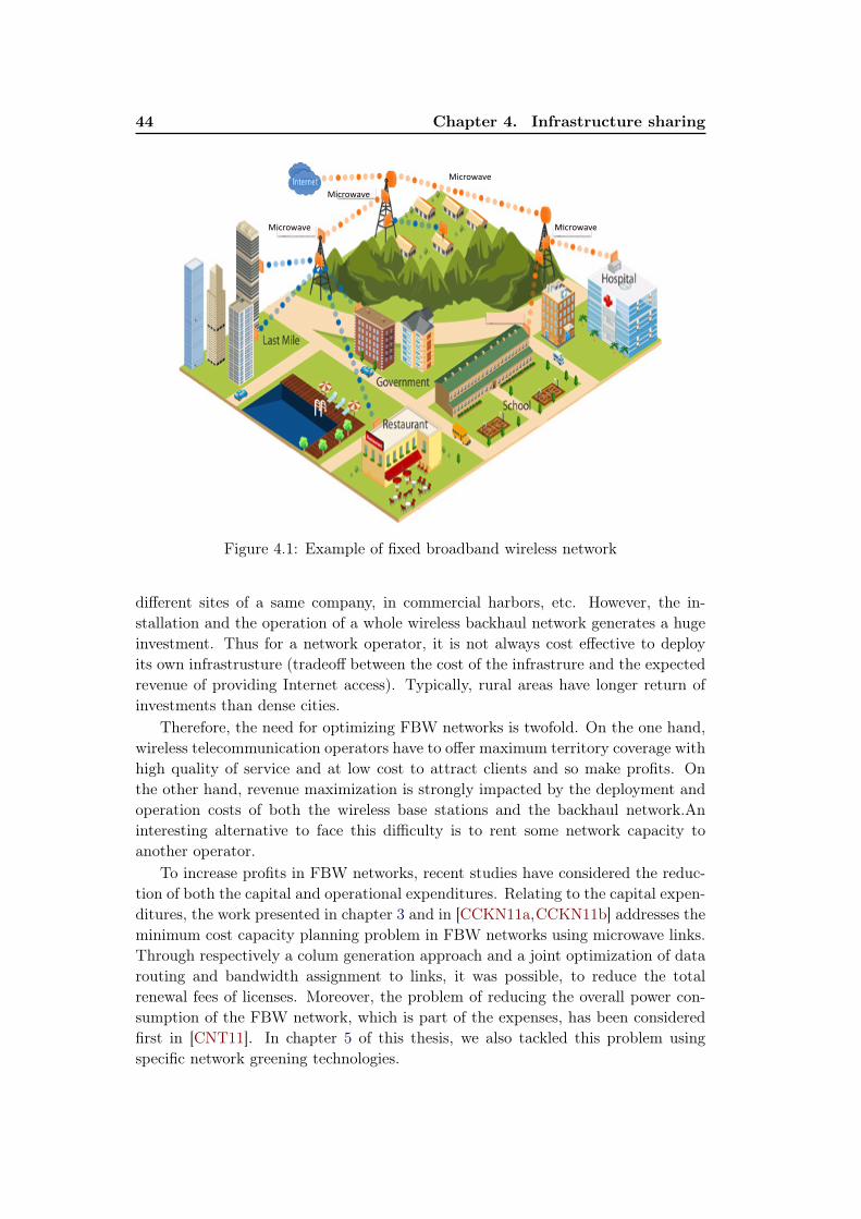
44 Chapter 4. Infrastructure sharing
Microwave
Microwave
Microwave
Microwave
Figure 4.1: Example of fixed broadband wireless network
different sites of a same company, in commercial harbors, etc. However, the in-stallation and the operation of a whole wireless backhaul network generates a hugeinvestment. Thus for a network operator, it is not always cost effective to deployits own infrastrusture (tradeoff between the cost of the infrastrure and the expectedrevenue of providing Internet access). Typically, rural areas have longer return ofinvestments than dense cities.
Therefore, the need for optimizing FBW networks is twofold. On the one hand,wireless telecommunication operators have to offer maximum territory coverage withhigh quality of service and at low cost to attract clients and so make profits. Onthe other hand, revenue maximization is strongly impacted by the deployment andoperation costs of both the wireless base stations and the backhaul network.Aninteresting alternative to face this difficulty is to rent some network capacity toanother operator.
To increase profits in FBW networks, recent studies have considered the reduc-tion of both the capital and operational expenditures. Relating to the capital expen-ditures, the work presented in chapter 3 and in [CCKN11a,CCKN11b] addresses theminimum cost capacity planning problem in FBW networks using microwave links.Through respectively a colum generation approach and a joint optimization of datarouting and bandwidth assignment to links, it was possible, to reduce the totalrenewal fees of licenses. Moreover, the problem of reducing the overall power con-sumption of the FBW network, which is part of the expenses, has been consideredfirst in [CNT11]. In chapter 5 of this thesis, we also tackled this problem usingspecific network greening technologies.
4.1. Introduction 45
In addition to these solutions, a new idea for optimizing FBW networks is toapply the concept of infrastructure sharing to generate new income. Infrastructuresharing consists in general, in renting some network equipments, such as sites, an-tennas or BTS, to other network operators. For instance, wireless base stations inremote areas with low traffic are often shared between operators to reduce invest-ment, and most of the high points where to install antennas are rented to dedicatedcompanies.
In this chapter, we assumed that the owner of the network infrastructure canlease the network capacity to others operators under commercial terms. Followingthe actual separation between infrastructure and services, we considered two kindsof network operators: the Physical Network Operator (PNO) that owns and oper-ates the FBW network infrastructure (antennas, radio links, etc.) and the VirtualNetwork Operator (VNO) that rents capacity from the PNO and uses the infras-tructure to deliver services to its clients. In fact, many network operators are ofboth kinds since it is hardly cost effective to fully deploy its own infrastructure forachieving full coverage of a country.
We considered that the service level agreement (SLA) signed between the PNOand a VNO includes not only quality-of-service (QoS) requirements such as delaysand satisfiability among concurrent flows, but also the capacity requirements overtime. Motivated by an efficient computation of the optimal solution of our problem,we first derived a mathematical formulation of the infrastructure sharing with SLAproblem with the objective of maximizing the PNO revenue. We then extendedthis formulation considering uncertain traffic demands, where aach demand has amean and peak value. To do so, we used the Γ-robustness approach mentionedin chapter 1. The Γ parameter here corresponds to the degree of robustness, i.e.the level of conservatism of the robust solution. This allows a better flexibilitythan traditional too conservative robust models like the model of Soyster. From apractical point of view, it is unlikely that all the VNO traffic requirements reachtheir peak value at the same time. Therefore we considered the case where thenumber of demands deviating from their mean value is bounded by Γ. Making Γ
vary from 0 to the total number of demands allows us to study the so-called priceof robustness, i.e. the additional price to pay in order to obtain a feasible solutionfor the robust scheme.
In Section 4.2, we carefully define the problem and present its mathematicalformulation when demands are considered static. Section 4.3 is devoted to therobust formulation adapted to the cases when demand requirements are consideredvariables. We report on computational results in Section 4.4 and we discuss themodel limits in Section 4.5. We then propose several methods to speed up theresolution in Section 4.6 and conclude with a perspective problem.
46 Chapter 4. Infrastructure sharing
4.2 Problem definition and nominal formulation
4.2.1 Problem situation
We consider a fixed broadband wireless network composed of multiple towers onwhich one or many Base Transciever Stations (BTS) are installed. Each BTS asexplained in the chapter 1 (Introduction) consists of three basic components: anindoor unit, an outdoor unit and the antenna used to transmit and receive thesignal into/from free space. Two BTS located on different towers can be connectedto each other with point-to-point wireless links, and two different BTS located onthe same tower are connected through a switch link connecting their indoor units.This network is owned by a PNO who wants to increase its revenue by sharing itsinfrastructure with interested VNOs. These latter are not willing at investing byconstructing their own networks but at serving their clients in the same geographicarea as the PNO. Together with the PNO, each VNO agrees n the SLA on itsamount of traffic requirements and the PNO’s revenue in case of satisfaction. Theyalso define the conditions of the VNO’s satisfaction and the level of QoS the PNOshould offer. The QoS parameter considered here is the end-to-end delay of eachdemand that should not exceed a predefined value. The goal of this study is todetermine the best set of VNOs that maximizes the total revenue of the PNO whilesatisfying all their constraints.
4.2.2 Static model formulation
We modeled our problem on a digraph G = (V,E) where V represents a set of towersand each link (u, v) ∈ E represents a fixed directed radio link from an antenna of aBTS located on node u to an antenna of a BTS located on node v. To each link (u, v)
is associated a capacity value Cuv. We were also given a set of n candidates VNOsand the traffic demand for a VNO q is represented by a set Dq = {(skq , tkq , dkq ), k =
1, . . . , |Dq|, q = 1, . . . , n} with skq , tkq and dkq respectively the source, the destinationand the volume of the kth demand of the qth VNO.
In order to efficiently compute the delay in the backhaul network, we made thefollowing two assumptions.
1. The propagation delay on a link (delay needed for a symbol to reach the recep-tion antenna from the emission one) is considered to be negligible regardingto its transmission delay in a router (delay needed to decode it, to send itfrom the antenna to the indoor unit, to treat it in the router, to send it toanother indoor unit, to re-code it and to send it to the antenna for emission).This hypothesis is based on the fact that in microwave networks, propagationdelays are in order of tens of microseconds (µs) while transmission delays arein order of milliseconds (ms) [Leh10].
2. We also consider the transmission delay of a unit of traffic demand in a routerof the infrastructure is known by advance and denoted by τ . It corresponds to
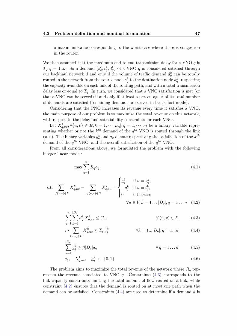
4.2. Problem definition and nominal formulation 47
a maximum value corresponding to the worst case where there is congestionin the router.
We then assumed that the maximum end-to-end transmission delay for a VNO q isTq, q = 1..n. So a demand (skq , t
kq , d
kq ) of a VNO q is considered satisfied through
our backhaul network if and only if the volume of traffic demand dkq can be totallyrouted in the network from the source node skq to the destination node dkq , respectingthe capacity available on each link of the routing path, and with a total transmissiondelay less or equal to Tq. In turn, we considered that a VNO satisfaction is met (orthat a VNO can be served) if and only if at least a percentage β of its total numberof demands are satisfied (remaining demands are served in best effort mode).
Considering that the PNO increases its revenue every time it satisfies a VNO,the main purpose of our problem is to maximize the total revenue on this network,with respect to the delay and satisfiability constraints for each VNO.
Let Xkq,uv, ∀{u, v} ∈ E, k = 1, · · · |Dq|, q = 1, · · · , n be a binary variable repre-
senting whether or not the kth demand of the qth VNO is routed through the link(u, v). The binary variables gkq and aq denote respectively the satisfaction of the kth
demand of the qth VNO, and the overall satisfaction of the qth VNO.From all considerations above, we formulated the problem with the following
integer linear model:
maxn∑q=1
Rqaq (4.1)
s.t.∑
v/(u,v)∈E
Xkq,uv −
∑v/(v,u)∈E
Xkq,vu =
gkq if u = skq ,
−gkq if u = tkq ,
0 otherwise
∀u ∈ V, k = 1 . . . |Dq|, q = 1 . . . n (4.2)
n∑q=1
|Dq |∑k=1
dkq Xkq,uv ≤ Cuv ∀ (u, v) ∈ E (4.3)
τ ·∑
(u,v)∈E
Xkq,uv ≤ Tq.gkq ∀k = 1...|Dq|, q = 1...n (4.4)
|Dq |∑k=1
gkq ≥ β|Dq|aq ∀ q = 1 . . . n (4.5)
aq, Xkq,uv, gkq ∈ {0, 1} (4.6)
The problem aims to maximize the total revenue of the network where Rq rep-resents the revenue associated to VNO q. Constraints (4.3) corresponds to thelink capacity constraints limiting the total amount of flow routed on a link, whileconstraint (4.2) ensures that the demand is routed on at most one path when thedemand can be satisfied. Constraints (4.4) are used to determine if a demand k is
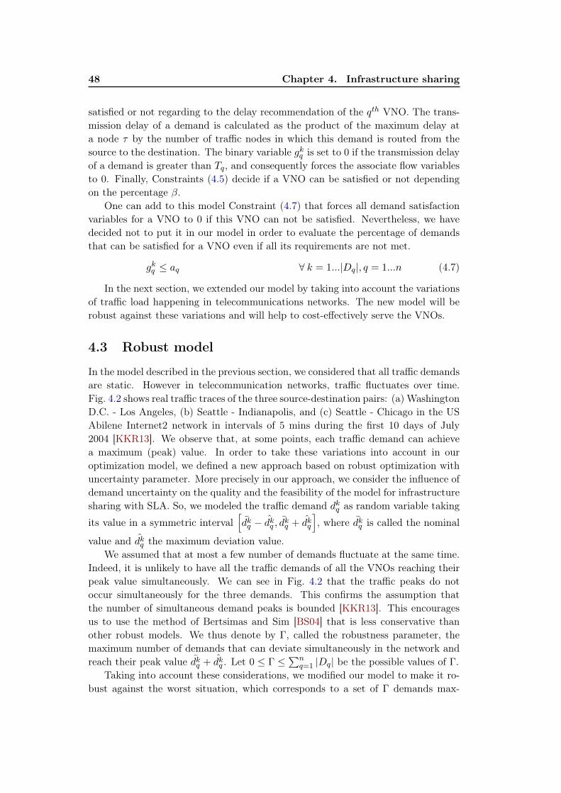
48 Chapter 4. Infrastructure sharing
satisfied or not regarding to the delay recommendation of the qth VNO. The trans-mission delay of a demand is calculated as the product of the maximum delay ata node τ by the number of traffic nodes in which this demand is routed from thesource to the destination. The binary variable gkq is set to 0 if the transmission delayof a demand is greater than Tq, and consequently forces the associate flow variablesto 0. Finally, Constraints (4.5) decide if a VNO can be satisfied or not dependingon the percentage β.
One can add to this model Constraint (4.7) that forces all demand satisfactionvariables for a VNO to 0 if this VNO can not be satisfied. Nevertheless, we havedecided not to put it in our model in order to evaluate the percentage of demandsthat can be satisfied for a VNO even if all its requirements are not met.
gkq ≤ aq ∀ k = 1...|Dq|, q = 1...n (4.7)
In the next section, we extended our model by taking into account the variationsof traffic load happening in telecommunications networks. The new model will berobust against these variations and will help to cost-effectively serve the VNOs.
4.3 Robust model
In the model described in the previous section, we considered that all traffic demandsare static. However in telecommunication networks, traffic fluctuates over time.Fig. 4.2 shows real traffic traces of the three source-destination pairs: (a) WashingtonD.C. - Los Angeles, (b) Seattle - Indianapolis, and (c) Seattle - Chicago in the USAbilene Internet2 network in intervals of 5 mins during the first 10 days of July2004 [KKR13]. We observe that, at some points, each traffic demand can achievea maximum (peak) value. In order to take these variations into account in ouroptimization model, we defined a new approach based on robust optimization withuncertainty parameter. More precisely in our approach, we consider the influence ofdemand uncertainty on the quality and the feasibility of the model for infrastructuresharing with SLA. So, we modeled the traffic demand dkq as random variable taking
its value in a symmetric interval[dkq − dkq , dkq + dkq
], where dkq is called the nominal
value and dkq the maximum deviation value.We assumed that at most a few number of demands fluctuate at the same time.
Indeed, it is unlikely to have all the traffic demands of all the VNOs reaching theirpeak value simultaneously. We can see in Fig. 4.2 that the traffic peaks do notoccur simultaneously for the three demands. This confirms the assumption thatthe number of simultaneous demand peaks is bounded [KKR13]. This encouragesus to use the method of Bertsimas and Sim [BS04] that is less conservative thanother robust models. We thus denote by Γ, called the robustness parameter, themaximum number of demands that can deviate simultaneously in the network andreach their peak value dkq + dkq . Let 0 ≤ Γ ≤
∑nq=1 |Dq| be the possible values of Γ.
Taking into account these considerations, we modified our model to make it ro-bust against the worst situation, which corresponds to a set of Γ demands max-
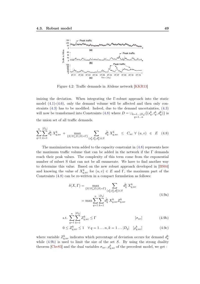
4.3. Robust model 49
Peak traffic
Peak traffic
Peak traffic
(a)
(b)
(c)
Figure 4.2: Traffic demands in Abilene network [KKR13]
imizing the deviation. When integrating the Γ-robust approach into the staticmodel (4.1)-(4.6), only the demand volume will be affected and then only con-straints (4.3) has to be modified. Indeed, due to the demand uncertainties, (4.3)will now be transformed into Constraints (4.8) where D = ∪k=1...|Dq |
q=1...n
{(skq , tkq , dkq )} is
the union set of all traffic demands.
n∑q=1
|Dq |∑k=1
dkq Xkq,uv + max
{S/S⊆D,|S|=Γ}
∑(skq ,t
kq ,d
kq )∈S
dkq Xkq,uv ≤ Cuv ∀ (u, v) ∈ E (4.8)
The maximization term added to the capacity constraint in (4.8) represents herethe maximum traffic volume that can be added in the network if the Γ demandsreach their peak values. The complexity of this term come from the exponentialnumber of subset S that can not be all enumerate. We have to find another wayto determine this value. Based on the new robust approach developed in [BS04]and knowing the value of Xk
q,uv for (u, v) ∈ E and Γ, the maximum part of theConstraints (4.8) can be re-written in a compact formulation as follows:
δ(X,Γ) = max{S/S⊆D,|S|=Γ}
∑(skq ,t
kq ,d
kq )∈S
dkq Xkq,uv
= maxn∑q=1
|Dq |∑k=1
dkq Xkq,uvZ
kq,uv
(4.9a)
s.t.n∑q=1
|Dq |∑k=1
Zkq,uv ≤ Γ [σuv] (4.9b)
0 ≤ Zkq,uv ≤ 1 ∀ q = 1 . . . n, k = 1 . . . |Dq| [ρkq,uv] (4.9c)
where variable Zkq,uv indicates which percentage of deviation occurs for demand dkqwhile (4.9b) is used to limit the size of the set S. By using the strong dualitytheorem [Chv83] and the dual variables σuv, ρkq,uv of the precedent model, we get :
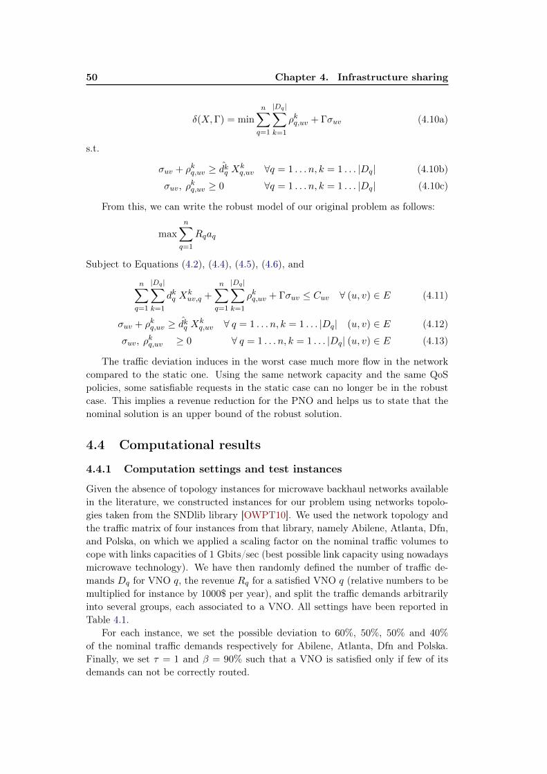
50 Chapter 4. Infrastructure sharing
δ(X,Γ) = minn∑q=1
|Dq |∑k=1
ρkq,uv + Γσuv (4.10a)
s.t.
σuv + ρkq,uv ≥ dkq Xkq,uv ∀q = 1 . . . n, k = 1 . . . |Dq| (4.10b)
σuv, ρkq,uv ≥ 0 ∀q = 1 . . . n, k = 1 . . . |Dq| (4.10c)
From this, we can write the robust model of our original problem as follows:
maxn∑q=1
Rqaq
Subject to Equations (4.2), (4.4), (4.5), (4.6), and
n∑q=1
|Dq |∑k=1
dkq Xkuv,q +
n∑q=1
|Dq |∑k=1
ρkq,uv + Γσuv ≤ Cuv ∀ (u, v) ∈ E (4.11)
σuv + ρkq,uv ≥ dkq Xkq,uv ∀ q = 1 . . . n, k = 1 . . . |Dq| (u, v) ∈ E (4.12)
σuv, ρkq,uv ≥ 0 ∀ q = 1 . . . n, k = 1 . . . |Dq| (u, v) ∈ E (4.13)
The traffic deviation induces in the worst case much more flow in the networkcompared to the static one. Using the same network capacity and the same QoSpolicies, some satisfiable requests in the static case can no longer be in the robustcase. This implies a revenue reduction for the PNO and helps us to state that thenominal solution is an upper bound of the robust solution.
4.4 Computational results
4.4.1 Computation settings and test instances
Given the absence of topology instances for microwave backhaul networks availablein the literature, we constructed instances for our problem using networks topolo-gies taken from the SNDlib library [OWPT10]. We used the network topology andthe traffic matrix of four instances from that library, namely Abilene, Atlanta, Dfn,and Polska, on which we applied a scaling factor on the nominal traffic volumes tocope with links capacities of 1 Gbits/sec (best possible link capacity using nowadaysmicrowave technology). We have then randomly defined the number of traffic de-mands Dq for VNO q, the revenue Rq for a satisfied VNO q (relative numbers to bemultiplied for instance by 1000$ per year), and split the traffic demands arbitrarilyinto several groups, each associated to a VNO. All settings have been reported inTable 4.1.
For each instance, we set the possible deviation to 60%, 50%, 50% and 40%of the nominal traffic demands respectively for Abilene, Atlanta, Dfn and Polska.Finally, we set τ = 1 and β = 90% such that a VNO is satisfied only if few of itsdemands can not be correctly routed.
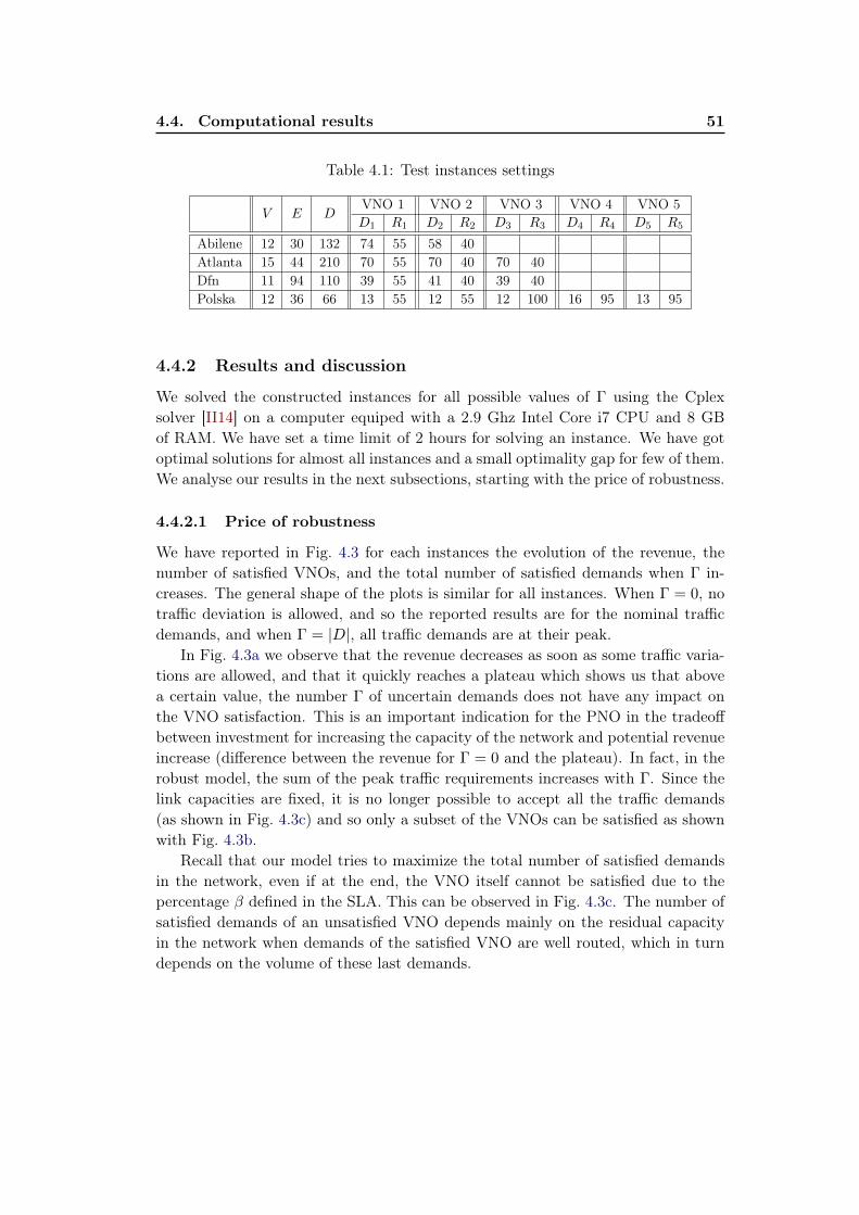
4.4. Computational results 51
Table 4.1: Test instances settings
V E DVNO 1 VNO 2 VNO 3 VNO 4 VNO 5D1 R1 D2 R2 D3 R3 D4 R4 D5 R5
Abilene 12 30 132 74 55 58 40Atlanta 15 44 210 70 55 70 40 70 40Dfn 11 94 110 39 55 41 40 39 40Polska 12 36 66 13 55 12 55 12 100 16 95 13 95
4.4.2 Results and discussion
We solved the constructed instances for all possible values of Γ using the Cplexsolver [II14] on a computer equiped with a 2.9 Ghz Intel Core i7 CPU and 8 GBof RAM. We have set a time limit of 2 hours for solving an instance. We have gotoptimal solutions for almost all instances and a small optimality gap for few of them.We analyse our results in the next subsections, starting with the price of robustness.
4.4.2.1 Price of robustness
We have reported in Fig. 4.3 for each instances the evolution of the revenue, thenumber of satisfied VNOs, and the total number of satisfied demands when Γ in-creases. The general shape of the plots is similar for all instances. When Γ = 0, notraffic deviation is allowed, and so the reported results are for the nominal trafficdemands, and when Γ = |D|, all traffic demands are at their peak.
In Fig. 4.3a we observe that the revenue decreases as soon as some traffic varia-tions are allowed, and that it quickly reaches a plateau which shows us that abovea certain value, the number Γ of uncertain demands does not have any impact onthe VNO satisfaction. This is an important indication for the PNO in the tradeoffbetween investment for increasing the capacity of the network and potential revenueincrease (difference between the revenue for Γ = 0 and the plateau). In fact, in therobust model, the sum of the peak traffic requirements increases with Γ. Since thelink capacities are fixed, it is no longer possible to accept all the traffic demands(as shown in Fig. 4.3c) and so only a subset of the VNOs can be satisfied as shownwith Fig. 4.3b.
Recall that our model tries to maximize the total number of satisfied demandsin the network, even if at the end, the VNO itself cannot be satisfied due to thepercentage β defined in the SLA. This can be observed in Fig. 4.3c. The number ofsatisfied demands of an unsatisfied VNO depends mainly on the residual capacityin the network when demands of the satisfied VNO are well routed, which in turndepends on the volume of these last demands.
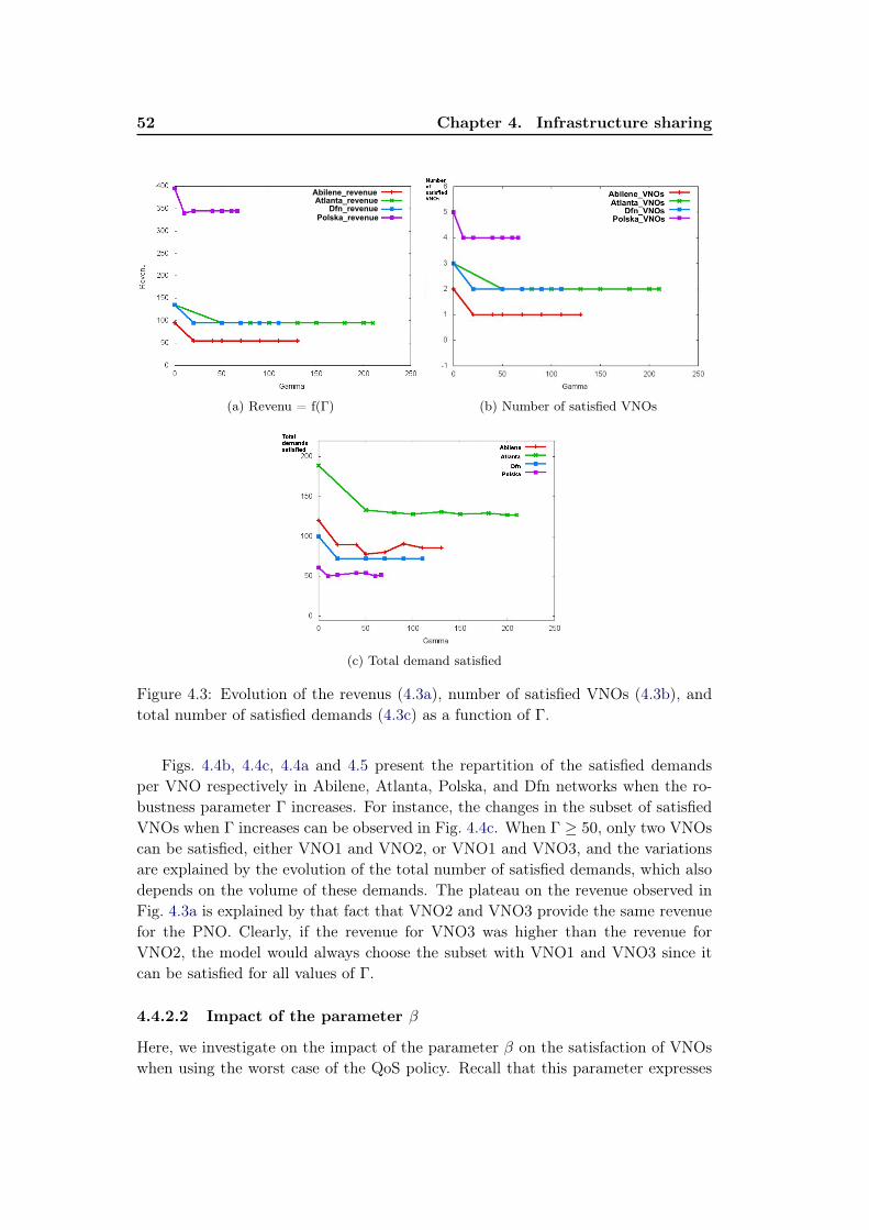
52 Chapter 4. Infrastructure sharing
Abilene_revenueAtlanta_revenue
Polska_revenueDfn_revenue
(a) Revenu = f(Γ) (b) Number of satisfied VNOs
(c) Total demand satisfied
Figure 4.3: Evolution of the revenus (4.3a), number of satisfied VNOs (4.3b), andtotal number of satisfied demands (4.3c) as a function of Γ.
Figs. 4.4b, 4.4c, 4.4a and 4.5 present the repartition of the satisfied demandsper VNO respectively in Abilene, Atlanta, Polska, and Dfn networks when the ro-bustness parameter Γ increases. For instance, the changes in the subset of satisfiedVNOs when Γ increases can be observed in Fig. 4.4c. When Γ ≥ 50, only two VNOscan be satisfied, either VNO1 and VNO2, or VNO1 and VNO3, and the variationsare explained by the evolution of the total number of satisfied demands, which alsodepends on the volume of these demands. The plateau on the revenue observed inFig. 4.3a is explained by that fact that VNO2 and VNO3 provide the same revenuefor the PNO. Clearly, if the revenue for VNO3 was higher than the revenue forVNO2, the model would always choose the subset with VNO1 and VNO3 since itcan be satisfied for all values of Γ.
4.4.2.2 Impact of the parameter β
Here, we investigate on the impact of the parameter β on the satisfaction of VNOswhen using the worst case of the QoS policy. Recall that this parameter expresses
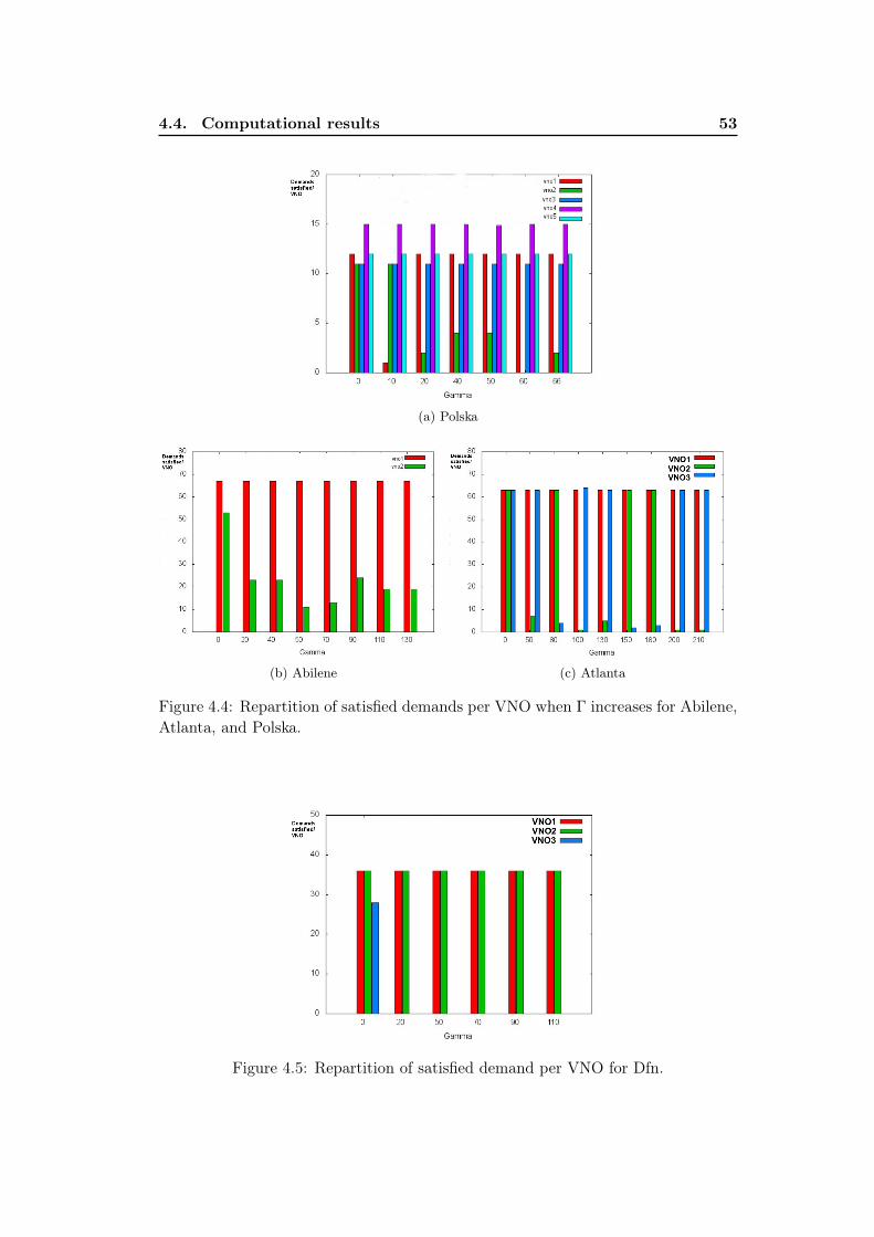
4.4. Computational results 53
(a) Polska
(b) Abilene (c) Atlanta
Figure 4.4: Repartition of satisfied demands per VNO when Γ increases for Abilene,Atlanta, and Polska.
Figure 4.5: Repartition of satisfied demand per VNO for Dfn.
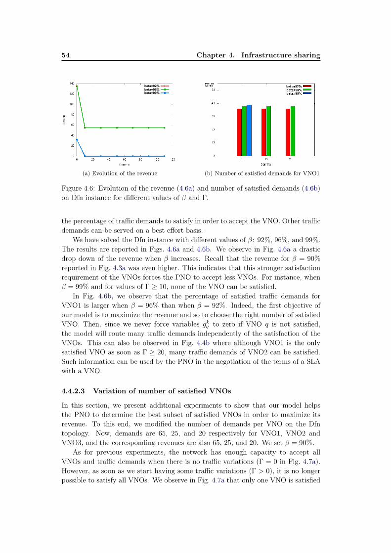
54 Chapter 4. Infrastructure sharing
beta=92%beta=96%beta=99%
(a) Evolution of the revenue (b) Number of satisfied demands for VNO1
Figure 4.6: Evolution of the revenue (4.6a) and number of satisfied demands (4.6b)on Dfn instance for different values of β and Γ.
the percentage of traffic demands to satisfy in order to accept the VNO. Other trafficdemands can be served on a best effort basis.
We have solved the Dfn instance with different values of β: 92%, 96%, and 99%.The results are reported in Figs. 4.6a and 4.6b. We observe in Fig. 4.6a a drasticdrop down of the revenue when β increases. Recall that the revenue for β = 90%
reported in Fig. 4.3a was even higher. This indicates that this stronger satisfactionrequirement of the VNOs forces the PNO to accept less VNOs. For instance, whenβ = 99% and for values of Γ ≥ 10, none of the VNO can be satisfied.
In Fig. 4.6b, we observe that the percentage of satisfied traffic demands forVNO1 is larger when β = 96% than when β = 92%. Indeed, the first objective ofour model is to maximize the revenue and so to choose the right number of satisfiedVNO. Then, since we never force variables gkq to zero if VNO q is not satisfied,the model will route many traffic demands independently of the satisfaction of theVNOs. This can also be observed in Fig. 4.4b where although VNO1 is the onlysatisfied VNO as soon as Γ ≥ 20, many traffic demands of VNO2 can be satisfied.Such information can be used by the PNO in the negotiation of the terms of a SLAwith a VNO.
4.4.2.3 Variation of number of satisfied VNOs
In this section, we present additional experiments to show that our model helpsthe PNO to determine the best subset of satisfied VNOs in order to maximize itsrevenue. To this end, we modified the number of demands per VNO on the Dfntopology. Now, demands are 65, 25, and 20 respectively for VNO1, VNO2 andVNO3, and the corresponding revenues are also 65, 25, and 20. We set β = 90%.
As for previous experiments, the network has enough capacity to accept allVNOs and traffic demands when there is no traffic variations (Γ = 0 in Fig. 4.7a).However, as soon as we start having some traffic variations (Γ > 0), it is no longerpossible to satisfy all VNOs. We observe in Fig. 4.7a that only one VNO is satisfied
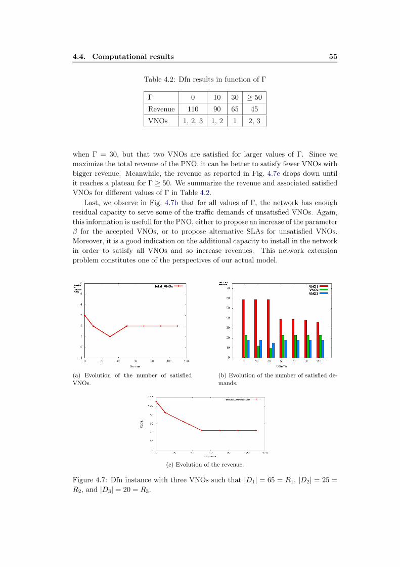
4.4. Computational results 55
Table 4.2: Dfn results in function of Γ
Γ 0 10 30 ≥ 50
Revenue 110 90 65 45
VNOs 1, 2, 3 1, 2 1 2, 3
when Γ = 30, but that two VNOs are satisfied for larger values of Γ. Since wemaximize the total revenue of the PNO, it can be better to satisfy fewer VNOs withbigger revenue. Meanwhile, the revenue as reported in Fig. 4.7c drops down untilit reaches a plateau for Γ ≥ 50. We summarize the revenue and associated satisfiedVNOs for different values of Γ in Table 4.2.
Last, we observe in Fig. 4.7b that for all values of Γ, the network has enoughresidual capacity to serve some of the traffic demands of unsatisfied VNOs. Again,this information is usefull for the PNO, either to propose an increase of the parameterβ for the accepted VNOs, or to propose alternative SLAs for unsatisfied VNOs.Moreover, it is a good indication on the additional capacity to install in the networkin order to satisfy all VNOs and so increase revenues. This network extensionproblem constitutes one of the perspectives of our actual model.
(a) Evolution of the number of satisfiedVNOs.
(b) Evolution of the number of satisfied de-mands.
total_revenue
(c) Evolution of the revenue.
Figure 4.7: Dfn instance with three VNOs such that |D1| = 65 = R1, |D2| = 25 =
R2, and |D3| = 20 = R3.
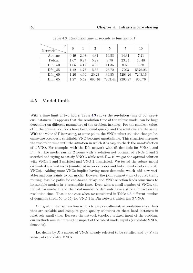
56 Chapter 4. Infrastructure sharing
Table 4.3: Resolution time in seconds as function of Γ
PPPPPPPPPNetworkΓ
0 1 3 5 7 10
Abilene 0.49 2.03 4.31 19.53 14.31 7.21Polska 1.67 9.27 5.28 8.78 23.24 16.48Dfn_50 1.05 4.17 4.99 11.35 8.66 6.38Dfn_55 1.12 4.77 5.55 26.72 7203 5576.23Dfn_60 1.20 4.69 20.23 39.55 7203.26 7203.16Dfn_65 1.27 5.52 683.46 7203.44 7203.27 860.76
4.5 Model limits
With a time limit of two hours, Table 4.3 shows the resolution time of our previ-ous instances. It appears that the resolution time of the robust model can be hugedepending on different parameters of the problem instance. For the smallest valuesof Γ, the optimal solutions have been found quickly and the solutions are the same.With the value of Γ increasing, at some point, the VNOs subset solution changes be-cause one previously satisfiable VNO becomes unsatisfiable. This situation increasesthe resolution time until the situation in which it is easy to check the unsatisfactionof a VNO. For example, with the Dfn network with 65 demands for VNO 1 andΓ = 5 , the model ran for 2 hours with a solution not optimal of VNOs 1 and 2satisfied and trying to satisfy VNO 3 while with Γ = 10 we got the optimal solutionwith VNOs 1 and 3 satisfied and VNO 2 unsatisfied. We tested the robust modelon limited size instances (number of network nodes and links, number of candidateVNOs). Adding more VNOs implies having more demands, which add new vari-ables and constraints to our model. However the joint computation of robust trafficrouting, feasible paths for end-to-end delay, and VNO selection leads sometimes tointractable models in a reasonable time. Even with a small number of VNOs, therobust parameter Γ and the total number of demands have a strong impact on theresolution time. That is the case when we considered in Table 4.3 different numberof demands (from 50 to 65) for VNO 1 in Dfn network which has 3 VNOs.
Our goal in the next section is thus to propose alternative resolution algorithmsthat are scalable and compute good quality solutions on these hard instances inrelatively small time. Because the network topology is fixed input of the problem,our methods aim at limiting the impact of the robust model inputs (candidate VNOs,demands).
Let define by X a subset of VNOs already selected to be satisfied and by Y thesubset of candidates VNOs.
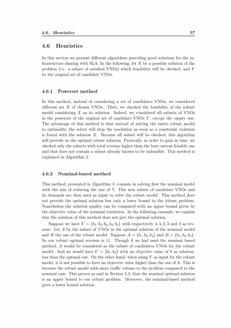
4.6. Heuristics 57
4.6 Heuristics
In this section we present different algorithms providing good solutions for the in-frastructure sharing with SLA. In the following, let X be a possible solution of theproblem (i.e. a subset of satisfied VNOs) which feasibility will be checked, and Ybe the original set of candidate VNOs.
4.6.1 Powerset method
In this method, instead of considering a set of candidates VNOs, we considereddifferent set X of chosen VNOs. Then, we checked the feasibility of the robustmodel considering X as its solution. Indeed, we considered all subsets of VNOsin the powerset of the original set of candidate VNOs Y , except the empty one.The advantage of this method is that instead of solving the entire robust modelto optimality, the solver will stop the resolution as soon as a constraint violationis found with the solution X. Because all subset will be checked, this algorithmwill provide us the optimal robust solution. Pratically, in order to gain in time, weckecked only the subsets with total revenue higher than the best current feasible oneand that does not contain a subset already known to be unfeasible. This method isexplained in Algorithm 2.
4.6.2 Nominal-based method
This method, presented in Algorithm 3, consists in solving first the nominal modelwith the aim of reducing the size of Y. This new subset of candidate VNOs andits demands are then used as input to solve the robust model. This method doesnot provide the optimal solution but only a lower bound to the robust problem.Nonetheless the solution quality can be compared with an upper bound given bythe objective value of the nominal resolution. In the following example, we explainwhy the solution of this method does not give the optimal solution.
Suppose we have Y = {b1, b2, b3, b4, b5} with respectively 4, 4, 2, 3 and 2 as rev-enue. Let A be the subset of VNOs in the optimal solution of the nominal modeland B the one of the robust model. Suppose A = {b1, b2, b4} and B = {b1, b2, b3}.So our robust optimal revenue is 11. Though if we had used the nominal basedmethod, A would be considered as the subset of candidates VNOs for the robustmodel. And we would have C = {b1, b2} with an objective value of 8 as solution,less than the optimal one. On the other hand, when using Y as input for the robustmodel, it is not possible to have an objective value higher than the one of A. This isbecause the robust model adds more traffic volume to the problem compared to thenominal case. This proves as said in Section 4.3, that the nominal optimal solutionis an upper bound to our robust problem. Moreover, the nominal-based methodgives a lower bound solution.
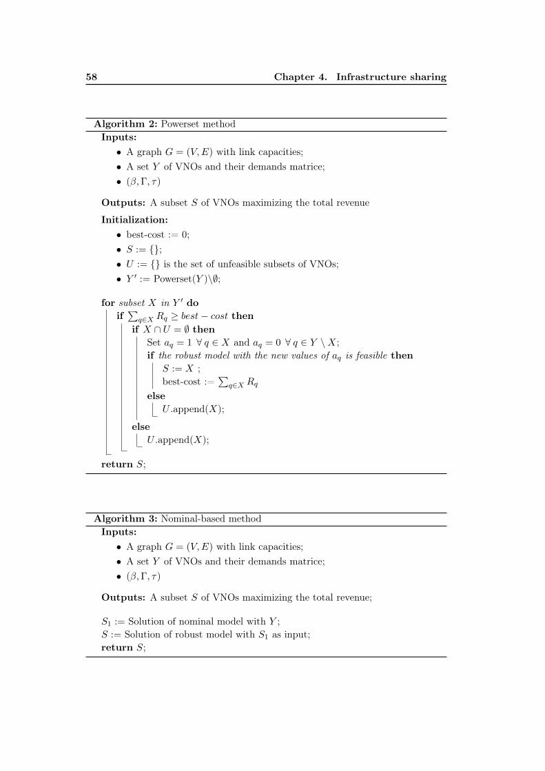
58 Chapter 4. Infrastructure sharing
Algorithm 2: Powerset methodInputs:• A graph G = (V,E) with link capacities;• A set Y of VNOs and their demands matrice;• (β,Γ, τ)
Outputs: A subset S of VNOs maximizing the total revenue
Initialization:• best-cost := 0;• S := {};• U := {} is the set of unfeasible subsets of VNOs;• Y ′ := Powerset(Y )\∅;
for subset X in Y ′ doif∑
q∈X Rq ≥ best− cost thenif X ∩ U = ∅ then
Set aq = 1 ∀ q ∈ X and aq = 0 ∀ q ∈ Y \X;if the robust model with the new values of aq is feasible then
S := X ;best-cost :=
∑q∈X Rq
elseU .append(X);
elseU .append(X);
return S;
Algorithm 3: Nominal-based methodInputs:• A graph G = (V,E) with link capacities;• A set Y of VNOs and their demands matrice;• (β,Γ, τ)
Outputs: A subset S of VNOs maximizing the total revenue;
S1 := Solution of nominal model with Y ;S := Solution of robust model with S1 as input;return S;
4.6. Heuristics 59
4.6.3 Greedy method
In this method, we searched for the best solution based on the price paid by a VNOwhen its satisfaction is met. The higher is this price paid by a VNO, the higher isthe PNO interest for him. We firstly sorted VNOs in the decreasing order of theirrevenue. Then, we searched for the best subset of VNOs S1 with the highest revenuethat is feasible for the robust model. As soon as S1 is found, at each iteration, weadded to it one VNO from those not in S1, starting from the one with the highestrevenue; and we checked the feasibility of this new subset. If it is not feasible, thenwe made the test with the next VNO otherwise we updated S1 before moving to thenext iteration. We iterated until all VNOs are checked. Once again, in this method,we just checked the feasibility of a predefined solution by finding a good routing.The heuristic is detailed in Algorithm 4.This method does not provide the optimal solution but a lower bound. For example,suppose we have found S1 with a revenue of 15 and that U = {b1, b2, b3, b4} withrespective revenues of 6, 4, 3 and 2. While testing the new VNOs subsets, we have:{{S1 + b1}, {S1 + b2 + b3}, {S1 + b2 + b4}} unsatisfiable and {S1 + b2} satisfied witha revenue of 19. At the same time, the subset {S1 + b3 + b4} with revenue 20 isalso satisfiable. The satisfaction of b2 in the greedy algorithm excludes the optimalsolution {S1 + b3 + b4}.
4.6.4 Heuristics performance
To evaluate the performance of our heuristics, we tested them on the last used Dfnnetwork with Γ = 5 and 7. It is the same instance as in Fig. 4.7. The robustresolution applied to this instance, with the solver, has run for more than 10000seconds without finding the optimal solution.
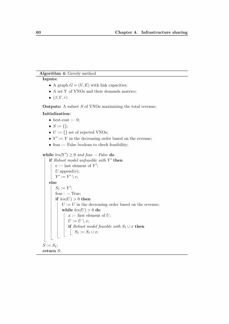
60 Chapter 4. Infrastructure sharing
Algorithm 4: Greedy methodInputs:• A graph G = (V,E) with link capacities;• A set Y of VNOs and their demands matrice;• (β,Γ, τ)
Outputs: A subset S of VNOs maximizing the total revenue;
Initialization:• best-cost := 0;• S := {};• U := {} set of rejected VNOs;• Y ′ := Y in the decreasing order based on the revenue;• feas := False boolean to check feasibility;
while len(Y ′) ≥ 0 and feas = False doif Robust model unfeasible with Y ′ then
e := last element of Y ′;U .append(e);Y ′ := Y ′ \ e;
elseS1 := Y ′;feas : = True;if len(U) > 0 then
U := U in the decreasing order based on the revenue;while len(U) > 0 do
x := first element of U ;U := U \ x;if Robust model feasible with S1 ∪ x then
S1 := S1 ∪ x;
S := S1;return S;
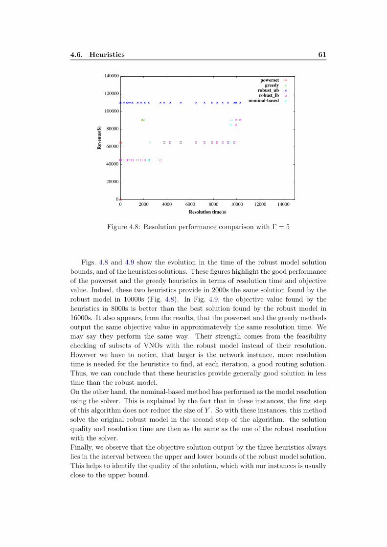
4.6. Heuristics 61
Figure 4.8: Resolution performance comparison with Γ = 5
Figs. 4.8 and 4.9 show the evolution in the time of the robust model solutionbounds, and of the heuristics solutions. These figures highlight the good performanceof the powerset and the greedy heuristics in terms of resolution time and objectivevalue. Indeed, these two heuristics provide in 2000s the same solution found by therobust model in 10000s (Fig. 4.8). In Fig. 4.9, the objective value found by theheuristics in 8000s is better than the best solution found by the robust model in16000s. It also appears, from the results, that the powerset and the greedy methodsoutput the same objective value in approximatevely the same resolution time. Wemay say they perform the same way. Their strength comes from the feasibilitychecking of subsets of VNOs with the robust model instead of their resolution.However we have to notice, that larger is the network instance, more resolutiontime is needed for the heuristics to find, at each iteration, a good routing solution.Thus, we can conclude that these heuristics provide generally good solution in lesstime than the robust model.On the other hand, the nominal-based method has performed as the model resolutionusing the solver. This is explained by the fact that in these instances, the first stepof this algorithm does not reduce the size of Y . So with these instances, this methodsolve the original robust model in the second step of the algorithm. the solutionquality and resolution time are then as the same as the one of the robust resolutionwith the solver.Finally, we observe that the objective solution output by the three heuristics alwayslies in the interval between the upper and lower bounds of the robust model solution.This helps to identify the quality of the solution, which with our instances is usuallyclose to the upper bound.
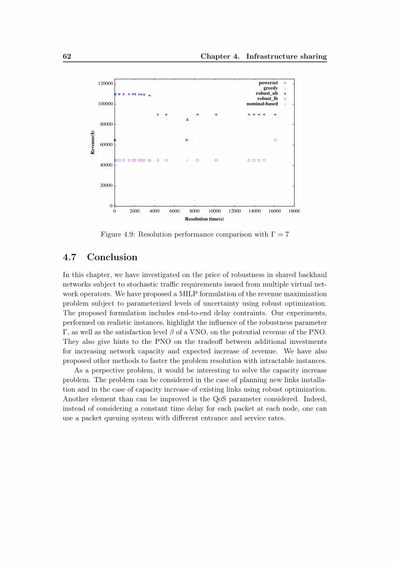
62 Chapter 4. Infrastructure sharing
Figure 4.9: Resolution performance comparison with Γ = 7
4.7 Conclusion
In this chapter, we have investigated on the price of robustness in shared backhaulnetworks subject to stochastic traffic requirements issued from multiple virtual net-work operators. We have proposed a MILP formulation of the revenue maximizationproblem subject to parameterized levels of uncertainty using robust optimization.The proposed formulation includes end-to-end delay contraints. Our experiments,performed on realistic instances, highlight the influence of the robustness parameterΓ, as well as the satisfaction level β of a VNO, on the potential revenue of the PNO.They also give hints to the PNO on the tradeoff between additional investmentsfor increasing network capacity and expected increase of revenue. We have alsoproposed other methods to faster the problem resolution with intractable instances.
As a perpective problem, it would be interesting to solve the capacity increaseproblem. The problem can be considered in the case of planning new links installa-tion and in the case of capacity increase of existing links using robust optimization.Another element than can be improved is the QoS parameter considered. Indeed,instead of considering a constant time delay for each packet at each node, one canuse a packet queuing system with different entrance and service rates.
Chapter 5
Energy-aware Routing inBackbone Networks
Contents5.1 Context and motivation . . . . . . . . . . . . . . . . . . . . . 645.2 Related Works . . . . . . . . . . . . . . . . . . . . . . . . . . . 66
5.2.1 Energy-aware Routing (EAR) . . . . . . . . . . . . . . . . . . 665.2.2 Redundancy Elimination . . . . . . . . . . . . . . . . . . . . . 685.2.3 GreenRE - Energy Savings with Redundancy Elimination . . 69
5.3 Robust-GreenRE Model . . . . . . . . . . . . . . . . . . . . . 725.3.1 Compact formulation . . . . . . . . . . . . . . . . . . . . . . 755.3.2 Constraint generation (Exact Algorithm) . . . . . . . . . . . 765.3.3 Heuristic Algorithm . . . . . . . . . . . . . . . . . . . . . . . 78
5.4 Computational Evaluation . . . . . . . . . . . . . . . . . . . . 805.4.1 Test instances and Experimental settings . . . . . . . . . . . 805.4.2 Results and Discussion . . . . . . . . . . . . . . . . . . . . . . 81
5.5 Conclusion . . . . . . . . . . . . . . . . . . . . . . . . . . . . . 89
The work of this chapter is motivated by the search of methods that can reducethe energy consumption of cellular mobile radio networks in order, firstly to makethem cost-effective and secondly to reduce the ICT impact on the global warming.Among the multiple approaches proposed in the litterature, we were interested inthe Energy Aware Routing (EAR) and the Redundancy Elimination (RE). Thesetechniques are applied to a backbone network with the goal to minimize its energyconsumption, even when variations in traffic load are registered.
We first model the problem in case of static traffic demands. The model combinesthe selection of the nodes where to install RE with EAR and so the minimizationof active links.
Then we extend the model to cope with fluctuations of trafficd and RE rate.We formulate this robust optimization problem as a Mixed Integer Linear Program(MILP). We also propose an efficient heuristic algorithm that is suitable for largenetworks.
We conduct a numerical evaluation of our models and heuristics using real traffictraces on Abilene, Geant and Germany50 networks. Our results show that ourapproach allows for 16-28% extra energy savings with respect to the classical EARmodel.
64 Chapter 5. Energy-aware Routing in Backbone Networks
5.1 Context and motivation
Recent studies have shown that ICT is responsible for 2% to 10% of the world-wide power consumption [Glo07,CMN11]. For example, the Global e-SustainabilityInitiative estimated the overall network energy requirement for European telecom-munication is around 35.8 TWh in 2020 [BDB+11]. The main consumers in cellularnetworks are data servers, backhaul routers and base stations (BS) which constitutesbetween 60 to 80% of the overall network power consumption [PVD+08]. With abase station consuming up to 700W during its active mode [PVD+08], backhaulnetwork represents a principal energy consumer and requires solutions to lower itspower consumption.Traditionally, networks are always designed to meet the peak-hour traffic demand.Therefore during normal periods, the traffic load is typically well below the net-work capacity. Following this observation, people have proposed, in the litterature,energy-aware routing (EAR) to minimize the number of used links while all thetraffic demands are routed without any overloaded links [CMN11,GS03, ZYLZ10].Another research topic that has also been active recently is traffic redundancy elim-ination (RE) [AGA+08,AMAR09, SGG10,ZCM11]. It consists in splitting packetsinto small chunks, each is indexed with a small key, that are cached along trafficflows as long as they are popular. Then, keys are substituted to chunks in trafficflows to avoid sending multiple times the same content, and the original data arerecovered on downstream routers based on the cache synchronization between thesending and the receiving routers. Therefore, traffic redundancy is removed andtraffic volumes of flows between the two routers are reduced. To apply RE to theBSs of a microwave backhaul networks, these infrastrusctures should be connected todevices having IP router functions. This is not yet the case today but a report con-ducted by Heavy Reading [HR13a,HR13b] on microwave backhaul evolution helpedto realise the wish of network operators (74% of those who answered) to have arouter connected to microwave node of their backhaul network that can apply L3protocols by 2016. This motivates us a good base to find an energy-aware routingsolution combined to RE technique for microwave backhaul network. Before thismethod could be tested with microwave backhaul networks, we use it to increasethe energy efficiency for IP backbone networks.In fact, in IP networks, the backbone and more precisely IP routers, are those thatconsume a majority of energy [TBA+08]. For simplicity, a traffic flow from whichredundancy has been removed is called a compressed flow. We use interchangeablythe notation compression rate or RE rate to denote how much traffic redundancycan be eliminated.
From energy savings perspective, RE has a drawback since it increases energyconsumption of routers [GMPR12]. To find a good trade-off, in [GMPR12], theauthors proposed GreenRE - a model that combines EAR and RE to increase energyefficiency for backbone network . In the GreenRE model, each of the demand hasa static traffic volume and is associated with a constant factor of redundant traffic.To handle future changes and guarantee a certain level of quality of service (QoS)
5.1. Context and motivation 65
(avoiding overloaded links), the peak volumes of traffic demand and the lowestRE rates are used as the worst case realization. Such assumption clearly leads toinefficient usage of network resources and poor energy savings. To alleviate thislimitation of the GreenRE model, we decided, here, to take into account in theoptimization process the uncertainty on traffic volumes and RE rates. By using thisextra information, we are able to obtain a design which would be closely relatedto the dynamics of the traffic pattern, hence significantly increase energy savingscompared to previous proposals.
In mathematical literature, the technology-independent Γ-robustness, presentedin Chapter 2, has been introduced in [BS03, BS04] and then successfully appliedto various network design problems [KKR13, CKPT13, CKS13]. This approach isbased on an observation that in real traffic traces, only a few of the demands aresimultaneously at their peaks. So, the authors considered a parameter Γ > 0 so thatat most Γ demands deviate simultaneously from their nominal traffic volumes. Basedon this assumption, the so-called robust solution is a solution that is feasible for anysubset of Γ demands simultaneously at their peaks, other demands are being at theirnominal values. The originality of the method is the expression of the maximumsum of deviation over all possible subsets of Γ demands as a unique linear program(LP). However, this LP formulation may have an exponential number of constraints.To overcome this issue, the LP formulation is transformed into a compact one usingthe duality theorem.
In the following, we first give a presentation of the EAR and RE concepts andtheir application in the research. Then we recall the definition and give a reformu-lation of the GreenRE model, which is the basis of our study. As contribution tothis work,
• First, we define and explain the impact of fluctuations in demands volumesand RE rates on the GreenRE formulation.
• Then we derive the robust model corresponding to ours problem using theΓ-robust model.
• Because of the exponential number of constraints in this model, we proposethree different methods to solve it. The first is a Mixed Integer Linear Program(MILP), called compact formulation, directly derived from the robust modelusing the duality property and some variables relaxations. Depending onthe problem instance, this method can provide the optimal solution, but ingeneral, it provides a lower bound of the energy savings. The second methodis an iterative algorithm, called Exact Algorithm. It aims at identifying thesubset of demands that will have the highest impact on the GReenRE modelwhen demands fluctuation are taken into account. It helps to find the exactvalue of the energy savings. The last method is a heuristic that is proposed toovercome the NP-Hardness of the Robust-GreenRE problem when applied tolarge instance. Its goal is to find a good quality solution in a relatively smallcomputation time.
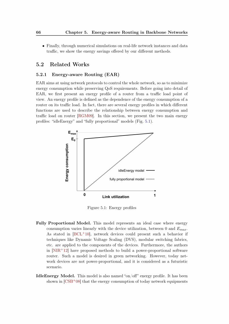
66 Chapter 5. Energy-aware Routing in Backbone Networks
• Finally, through numerical simulations on real-life network instances and datatraffic, we show the energy savings offered by our different methods.
5.2 Related Works
5.2.1 Energy-aware Routing (EAR)
EAR aims at using network protocols to control the whole network, so as to minimizeenergy consumption while preserving QoS requirements. Before going into detail ofEAR, we first present an energy profile of a router from a traffic load point ofview. An energy profile is defined as the dependence of the energy consumption of arouter on its traffic load. In fact, there are several energy profiles in which differentfunctions are used to describe the relationship between energy consumption andtraffic load on router [RGM09]. In this section, we present the two main energyprofiles: “idleEnergy” and “fully proportional” models (Fig. 5.1).
E0
Emax
Link utilization0 1
En
erg
y c
on
su
mp
tio
n
idleEnergy model
fully proportional model
Figure 5.1: Energy profiles
Fully Proportional Model. This model represents an ideal case where energyconsumption varies linearly with the device utilization, between 0 and Emax.As stated in [BCL+10], network devices could present such a behavior iftechniques like Dynamic Voltage Scaling (DVS), modular switching fabrics,etc. are applied to the components of the devices. Furthermore, the authorsin [NIR+12] have proposed methods to build a power-proportional softwarerouter. Such a model is desired in green networking. However, today net-work devices are not power-proportional, and it is considered as a futuristicscenario.
IdleEnergy Model. This model is also named “on/off” energy profile. It has beenshown in [CSB+08] that the energy consumption of today network equipments
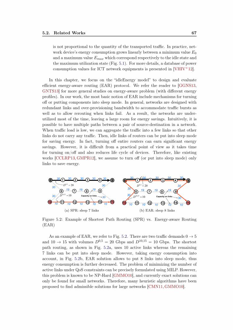
5.2. Related Works 67
is not proportional to the quantity of the transported traffic. In practice, net-work device’s energy consumption grows linearly between a minimum value E0
and a maximum value Emax which correspond respectively to the idle state andthe maximum utilization state (Fig. 5.1). For more details, a database of powerconsumption values for ICT network equipments is presented in [VHIV+12].
In this chapter, we focus on the “idleEnergy model” to design and evaluateefficient energy-aware routing (EAR) protocol. We refer the reader to [GGNS13,GNTS13] for more general studies on energy-aware problem (with different energyprofiles). In our work, the most basic notion of EAR include mechanisms for turningoff or putting components into sleep mode. In general, networks are designed withredundant links and over-provisioning bandwidth to accommodate traffic bursts aswell as to allow rerouting when links fail. As a result, the networks are under-utilized most of the time, leaving a large room for energy savings. Intuitively, it ispossible to have multiple paths between a pair of source-destination in a network.When traffic load is low, we can aggregate the traffic into a few links so that otherlinks do not carry any traffic. Then, idle links of routers can be put into sleep modefor saving energy. In fact, turning off entire routers can earn significant energysavings. However, it is difficult from a practical point of view as it takes timefor turning on/off and also reduces life cycle of devices. Therefore, like existingworks [CCLRP13,GMPR12], we assume to turn off (or put into sleep mode) onlylinks to save energy.
0
6 87
10
9
30 30 30 30
30
19 19 19
30
1010 10 10 10
5
15
30
3030
Capacity on links
1 2 3 4
11 12 13 14
0,520D =
10,1510D =
(a) SPR: sleep 7 links
6 87
10
9
11 12 13 14
30 30 30 30
30
19 19 19
30
1010 10 10 10
5
15
30
30
30
Capacity on links
0 1 2 3 4
0,520D =
10,1510D =
(b) EAR: sleep 8 links
Figure 5.2: Example of Shortest Path Routing (SPR) vs. Energy-aware Routing(EAR)
As an example of EAR, we refer to Fig. 5.2. There are two traffic demands 0→ 5
and 10 → 15 with volumes D0,5 = 20 Gbps and D10,15 = 10 Gbps. The shortestpath routing, as shown in Fig. 5.2a, uses 10 active links whereas the remaining7 links can be put into sleep mode. However, taking energy consumption intoaccount, in Fig. 5.2b, EAR solution allows to put 8 links into sleep mode, thusenergy consumption is further decreased. The problem of minimizing the number ofactive links under QoS constraints can be precisely formulated using MILP. However,this problem is known to be NP-Hard [GMMO10], and currently exact solutions canonly be found for small networks. Therefore, many heuristic algorithms have beenproposed to find admissible solutions for large networks [CMN11,GMMO10].
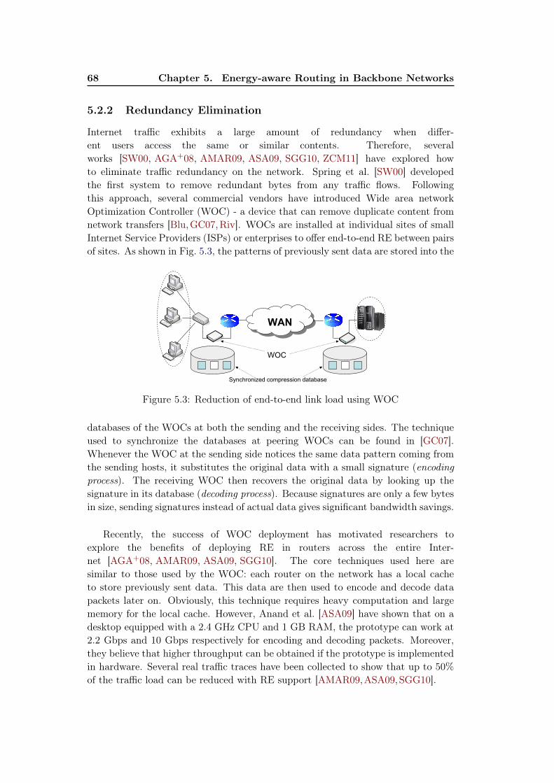
68 Chapter 5. Energy-aware Routing in Backbone Networks
5.2.2 Redundancy Elimination
Internet traffic exhibits a large amount of redundancy when differ-ent users access the same or similar contents. Therefore, severalworks [SW00, AGA+08, AMAR09, ASA09, SGG10, ZCM11] have explored howto eliminate traffic redundancy on the network. Spring et al. [SW00] developedthe first system to remove redundant bytes from any traffic flows. Followingthis approach, several commercial vendors have introduced Wide area networkOptimization Controller (WOC) - a device that can remove duplicate content fromnetwork transfers [Blu,GC07,Riv]. WOCs are installed at individual sites of smallInternet Service Providers (ISPs) or enterprises to offer end-to-end RE between pairsof sites. As shown in Fig. 5.3, the patterns of previously sent data are stored into the
WAN
` WOC
Synchronized compression database
Figure 5.3: Reduction of end-to-end link load using WOC
databases of the WOCs at both the sending and the receiving sides. The techniqueused to synchronize the databases at peering WOCs can be found in [GC07].Whenever the WOC at the sending side notices the same data pattern coming fromthe sending hosts, it substitutes the original data with a small signature (encodingprocess). The receiving WOC then recovers the original data by looking up thesignature in its database (decoding process). Because signatures are only a few bytesin size, sending signatures instead of actual data gives significant bandwidth savings.
Recently, the success of WOC deployment has motivated researchers toexplore the benefits of deploying RE in routers across the entire Inter-net [AGA+08, AMAR09, ASA09, SGG10]. The core techniques used here aresimilar to those used by the WOC: each router on the network has a local cacheto store previously sent data. This data are then used to encode and decode datapackets later on. Obviously, this technique requires heavy computation and largememory for the local cache. However, Anand et al. [ASA09] have shown that on adesktop equipped with a 2.4 GHz CPU and 1 GB RAM, the prototype can work at2.2 Gbps and 10 Gbps respectively for encoding and decoding packets. Moreover,they believe that higher throughput can be obtained if the prototype is implementedin hardware. Several real traffic traces have been collected to show that up to 50%of the traffic load can be reduced with RE support [AMAR09,ASA09,SGG10].
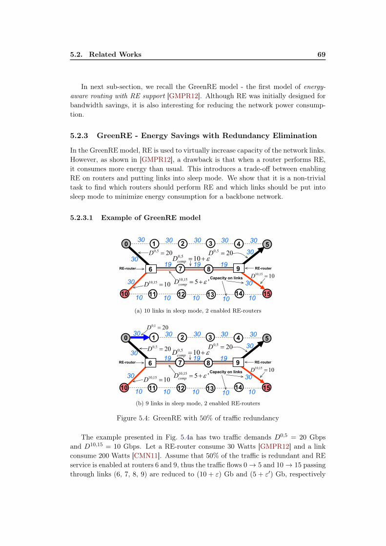
5.2. Related Works 69
In next sub-section, we recall the GreenRE model - the first model of energy-aware routing with RE support [GMPR12]. Although RE was initially designed forbandwidth savings, it is also interesting for reducing the network power consump-tion.
5.2.3 GreenRE - Energy Savings with Redundancy Elimination
In the GreenRE model, RE is used to virtually increase capacity of the network links.However, as shown in [GMPR12], a drawback is that when a router performs RE,it consumes more energy than usual. This introduces a trade-off between enablingRE on routers and putting links into sleep mode. We show that it is a non-trivialtask to find which routers should perform RE and which links should be put intosleep mode to minimize energy consumption for a backbone network.
5.2.3.1 Example of GreenRE model
0 1 2 3 4
10 11 12 13 14
30 30 30 30
30
19 19 19
30
1010 10 10 10
5
15
30
30
30
Capacity on links
RE-router RE-router7 86 9
0,520D =
10,1510D =
10,1510D =
0,520D =
0,510
compD ε= +
10,155 '
compD ε= +
(a) 10 links in sleep mode, 2 enabled RE-routers
0 1 2 3 4
10 11 12 13 14
30 30 30 30
30
19 19 19
30
1010 10 10 10
5
15
30
30
30
Capacity on links
RE-router RE-router7 86 9
0,520D =
10,1510D =
10,1510D =
0,520D =
0,120D =
0,510
compD ε= +
10,155 '
compD ε= +
(b) 9 links in sleep mode, 2 enabled RE-routers
Figure 5.4: GreenRE with 50% of traffic redundancy
The example presented in Fig. 5.4a has two traffic demands D0,5 = 20 Gbpsand D10,15 = 10 Gbps. Let a RE-router consume 30 Watts [GMPR12] and a linkconsume 200 Watts [CMN11]. Assume that 50% of the traffic is redundant and REservice is enabled at routers 6 and 9, thus the traffic flows 0→ 5 and 10→ 15 passingthrough links (6, 7, 8, 9) are reduced to (10 + ε) Gb and (5 + ε′) Gb, respectively
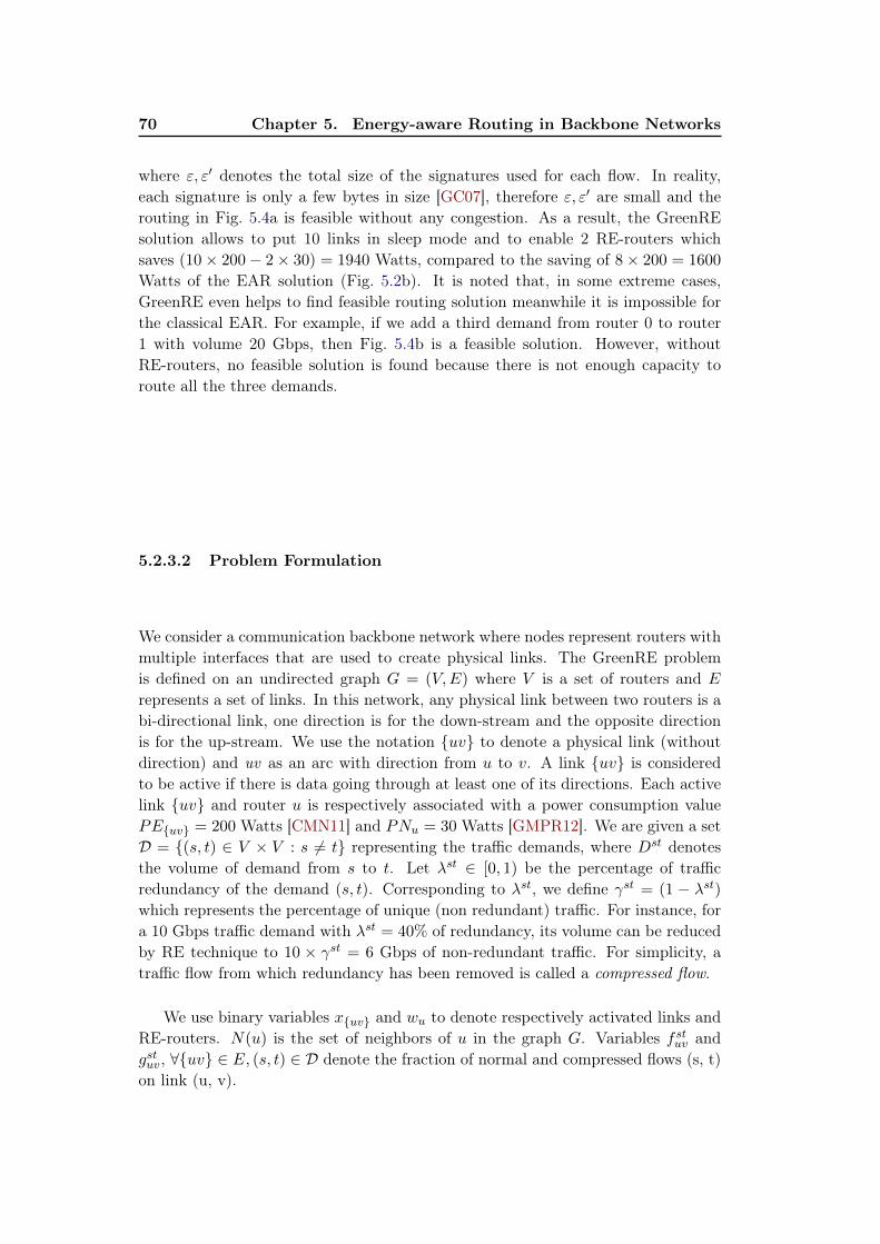
70 Chapter 5. Energy-aware Routing in Backbone Networks
where ε, ε′ denotes the total size of the signatures used for each flow. In reality,each signature is only a few bytes in size [GC07], therefore ε, ε′ are small and therouting in Fig. 5.4a is feasible without any congestion. As a result, the GreenREsolution allows to put 10 links in sleep mode and to enable 2 RE-routers whichsaves (10× 200− 2× 30) = 1940 Watts, compared to the saving of 8× 200 = 1600
Watts of the EAR solution (Fig. 5.2b). It is noted that, in some extreme cases,GreenRE even helps to find feasible routing solution meanwhile it is impossible forthe classical EAR. For example, if we add a third demand from router 0 to router1 with volume 20 Gbps, then Fig. 5.4b is a feasible solution. However, withoutRE-routers, no feasible solution is found because there is not enough capacity toroute all the three demands.
5.2.3.2 Problem Formulation
We consider a communication backbone network where nodes represent routers withmultiple interfaces that are used to create physical links. The GreenRE problemis defined on an undirected graph G = (V,E) where V is a set of routers and E
represents a set of links. In this network, any physical link between two routers is abi-directional link, one direction is for the down-stream and the opposite directionis for the up-stream. We use the notation {uv} to denote a physical link (withoutdirection) and uv as an arc with direction from u to v. A link {uv} is consideredto be active if there is data going through at least one of its directions. Each activelink {uv} and router u is respectively associated with a power consumption valuePE{uv} = 200 Watts [CMN11] and PNu = 30 Watts [GMPR12]. We are given a setD = {(s, t) ∈ V × V : s 6= t} representing the traffic demands, where Dst denotesthe volume of demand from s to t. Let λst ∈ [0, 1) be the percentage of trafficredundancy of the demand (s, t). Corresponding to λst, we define γst = (1 − λst)which represents the percentage of unique (non redundant) traffic. For instance, fora 10 Gbps traffic demand with λst = 40% of redundancy, its volume can be reducedby RE technique to 10 × γst = 6 Gbps of non-redundant traffic. For simplicity, atraffic flow from which redundancy has been removed is called a compressed flow.
We use binary variables x{uv} and wu to denote respectively activated links andRE-routers. N(u) is the set of neighbors of u in the graph G. Variables fstuv andgstuv, ∀{uv} ∈ E, (s, t) ∈ D denote the fraction of normal and compressed flows (s, t)on link (u, v).
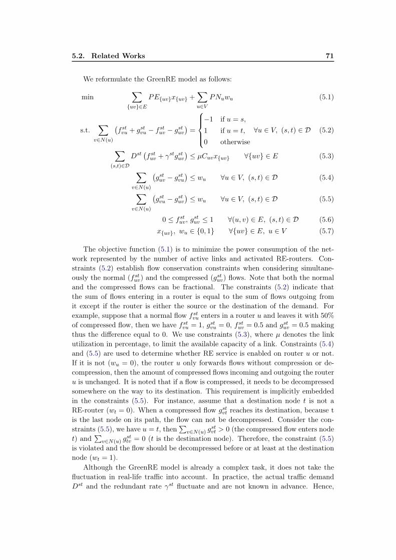
5.2. Related Works 71
We reformulate the GreenRE model as follows:
min∑{uv}∈E
PE{uv}x{uv} +∑u∈V
PNuwu (5.1)
s.t.∑
v∈N(u)
(fstvu + gstvu − fstuv − gstuv
)=
−1 if u = s,
1 if u = t,
0 otherwise
∀u ∈ V, (s, t) ∈ D (5.2)
∑(s,t)∈D
Dst(fstuv + γstgstuv
)≤ µCuvx{uv} ∀{uv} ∈ E (5.3)
∑v∈N(u)
(gstuv − gstvu
)≤ wu ∀u ∈ V, (s, t) ∈ D (5.4)
∑v∈N(u)
(gstvu − gstuv
)≤ wu ∀u ∈ V, (s, t) ∈ D (5.5)
0 ≤ fstuv, gstuv ≤ 1 ∀(u, v) ∈ E, (s, t) ∈ D (5.6)
x{uv}, wu ∈ {0, 1} ∀{uv} ∈ E, u ∈ V (5.7)
The objective function (5.1) is to minimize the power consumption of the net-work represented by the number of active links and activated RE-routers. Con-straints (5.2) establish flow conservation constraints when considering simultane-ously the normal (fstuv) and the compressed (gstuv) flows. Note that both the normaland the compressed flows can be fractional. The constraints (5.2) indicate thatthe sum of flows entering in a router is equal to the sum of flows outgoing fromit except if the router is either the source or the destination of the demand. Forexample, suppose that a normal flow fstvu enters in a router u and leaves it with 50%
of compressed flow, then we have fstvu = 1, gstvu = 0, fstuv = 0.5 and gstuv = 0.5 makingthus the difference equal to 0. We use constraints (5.3), where µ denotes the linkutilization in percentage, to limit the available capacity of a link. Constraints (5.4)and (5.5) are used to determine whether RE service is enabled on router u or not.If it is not (wu = 0), the router u only forwards flows without compression or de-compression, then the amount of compressed flows incoming and outgoing the routeru is unchanged. It is noted that if a flow is compressed, it needs to be decompressedsomewhere on the way to its destination. This requirement is implicitly embeddedin the constraints (5.5). For instance, assume that a destination node t is not aRE-router (wt = 0). When a compressed flow gstvt reaches its destination, because tis the last node on its path, the flow can not be decompressed. Consider the con-straints (5.5), we have u = t, then
∑v∈N(u) g
stvt > 0 (the compressed flow enters node
t) and∑
v∈N(u) gsttv = 0 (t is the destination node). Therefore, the constraint (5.5)
is violated and the flow should be decompressed before or at least at the destinationnode (wt = 1).
Although the GreenRE model is already a complex task, it does not take thefluctuation in real-life traffic into account. In practice, the actual traffic demandDst and the redundant rate γst fluctuate and are not known in advance. Hence,
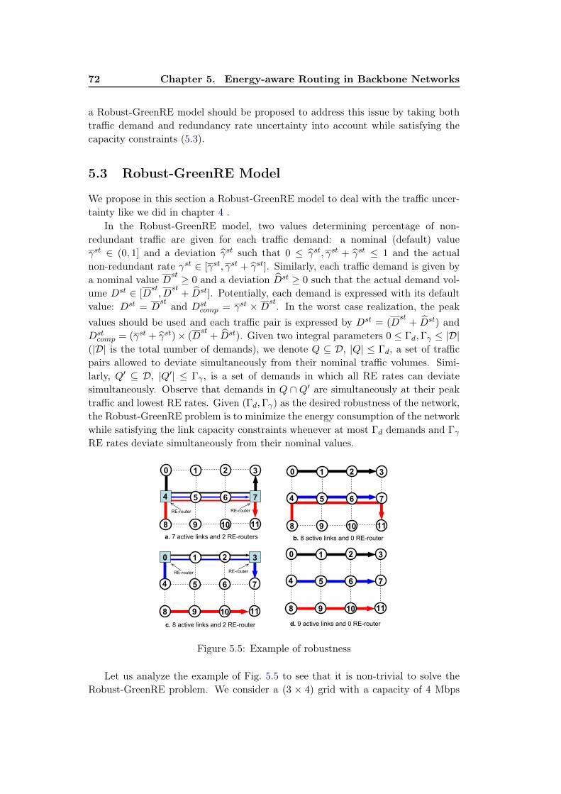
72 Chapter 5. Energy-aware Routing in Backbone Networks
a Robust-GreenRE model should be proposed to address this issue by taking bothtraffic demand and redundancy rate uncertainty into account while satisfying thecapacity constraints (5.3).
5.3 Robust-GreenRE Model
We propose in this section a Robust-GreenRE model to deal with the traffic uncer-tainty like we did in chapter 4 .
In the Robust-GreenRE model, two values determining percentage of non-redundant traffic are given for each traffic demand: a nominal (default) valueγst ∈ (0, 1] and a deviation γst such that 0 ≤ γst, γst + γst ≤ 1 and the actualnon-redundant rate γst ∈ [γst, γst + γst]. Similarly, each traffic demand is given bya nominal value Dst ≥ 0 and a deviation Dst ≥ 0 such that the actual demand vol-ume Dst ∈ [D
st, D
st+ Dst]. Potentially, each demand is expressed with its default
value: Dst = Dst and Dst
comp = γst × Dst. In the worst case realization, the peakvalues should be used and each traffic pair is expressed by Dst = (D
st+ Dst) and
Dstcomp = (γst + γst)× (D
st+ Dst). Given two integral parameters 0 ≤ Γd,Γγ ≤ |D|
(|D| is the total number of demands), we denote Q ⊆ D, |Q| ≤ Γd, a set of trafficpairs allowed to deviate simultaneously from their nominal traffic volumes. Simi-larly, Q′ ⊆ D, |Q′| ≤ Γγ , is a set of demands in which all RE rates can deviatesimultaneously. Observe that demands in Q ∩ Q′ are simultaneously at their peaktraffic and lowest RE rates. Given (Γd,Γγ) as the desired robustness of the network,the Robust-GreenRE problem is to minimize the energy consumption of the networkwhile satisfying the link capacity constraints whenever at most Γd demands and ΓγRE rates deviate simultaneously from their nominal values.
a. 7 active links and 2 RE-routers
0
10
5
1 2 3
11
6
8 9
0
10
5
1 2 3
4
11
6 7
8 9
4 7
RE-router RE-router
10
5
1 2
4
11
6 7
8 9
b. 8 active links and 0 RE-router
c. 8 active links and 2 RE-router
0
10
5
1 2 3
4
11
6 7
8 9
d. 9 active links and 0 RE-router
0 3
RE-router RE-router
Figure 5.5: Example of robustness
Let us analyze the example of Fig. 5.5 to see that it is non-trivial to solve theRobust-GreenRE problem. We consider a (3 × 4) grid with a capacity of 4 Mbps
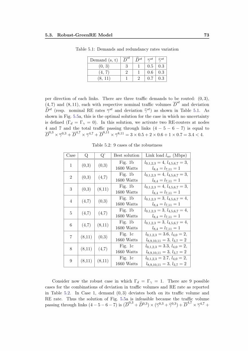
5.3. Robust-GreenRE Model 73
Table 5.1: Demands and redundancy rates variation
Demand (s, t) Dst
Dst γst γst
(0, 3) 3 1 0.5 0.3(4, 7) 2 1 0.6 0.3(8, 11) 1 2 0.7 0.3
per direction of each links. There are three traffic demands to be routed: (0, 3),(4, 7) and (8, 11), each with respective nominal traffic volumes Dst and deviationDst (resp. nominal RE rates γst and deviation γst) as shown in Table 5.1. Asshown in Fig. 5.5a, this is the optimal solution for the case in which no uncertaintyis defined (Γd = Γγ = 0). In this solution, we activate two RE-routers at nodes4 and 7 and the total traffic passing through links (4 − 5 − 6 − 7) is equal toD
0,3 × γ0,3 +D4,7 × γ4,7 +D
8,11 × γ8,11 = 3× 0.5 + 2× 0.6 + 1× 0.7 = 3.4 < 4.
Table 5.2: 9 cases of the robustness
Case Q Q’ Best solution Link load luv (Mbps)
1 (0,3) (0,3)Fig. 1b l0,1,2,3 = 4, l4,5,6,7 = 3,
1600 Watts l8,4 = l7,11 = 1
2 (0,3) (4,7)Fig. 1b l0,1,2,3 = 4, l4,5,6,7 = 3,
1600 Watts l8,4 = l7,11 = 1
3 (0,3) (8,11)Fig. 1b l0,1,2,3 = 4, l4,5,6,7 = 3,
1600 Watts l8,4 = l7,11 = 1
4 (4,7) (0,3)Fig. 1b l0,1,2,3 = 3, l4,5,6,7 = 4,
1600 Watts l8,4 = l7,11 = 1
5 (4,7) (4,7)Fig. 1b l0,1,2,3 = 3, l4,5,6,7 = 4,
1600 Watts l8,4 = l7,11 = 1
6 (4,7) (8,11)Fig. 1b l0,1,2,3 = 3, l4,5,6,7 = 4,
1600 Watts l8,4 = l7,11 = 1
7 (8,11) (0,3)Fig. 1c l0,1,2,3 = 3.6, l4,0 = 2,
1660 Watts l8,9,10,11 = 3, l3,7 = 2
8 (8,11) (4,7)Fig. 1c l0,1,2,3 = 3.3, l4,0 = 2,
1660 Watts l8,9,10,11 = 3, l3,7 = 2
9 (8,11) (8,11)Fig. 1c l0,1,2,3 = 2.7, l4,0 = 2,
1660 Watts l8,9,10,11 = 3, l3,7 = 2
Consider now the robust case in which Γd = Γγ = 1. There are 9 possiblecases for the combinations of deviation in traffic volumes and RE rate as reportedin Table 5.2. In Case 1, demand (0, 3) deviates both on its traffic volume andRE rate. Thus the solution of Fig. 5.5a is infeasible because the traffic volumepassing through links (4− 5− 6− 7) is (D
0,3+ D0,3)× (γ0,3 + γ0,3) +D
4,7 × γ4,7 +
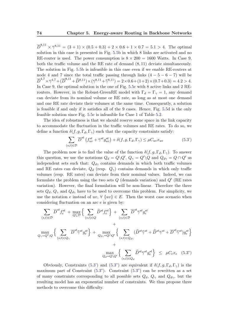
74 Chapter 5. Energy-aware Routing in Backbone Networks
D8,11 × γ8,11 = (3 + 1) × (0.5 + 0.3) + 2 × 0.6 + 1 × 0.7 = 5.1 > 4. The optimal
solution in this case is presented in Fig. 5.5b in which 8 links are activated and noRE-router is used. The power consumption is 8 × 200 = 1600 Watts. In Case 9,both the traffic volume and the RE rate of demand (8, 11) deviate simultaneously.The solution in Fig. 5.5b is infeasible in this case even if we enable RE-routers atnode 4 and 7 since the total traffic passing through links (4 − 5 − 6 − 7) will beD
4,7×γ4,7 +(D8,11
+D8,11)×(γ8,11 + γ8,11) = 2×0.6+(1+2)×(0.7+0.3) = 4.2 > 4.In Case 9, the optimal solution is the one of Fig. 5.5c with 8 active links and 2 RE-routers. However, in the Robust-GreenRE model with Γd = Γγ = 1, any demandcan deviate from its nominal volume or RE rate, as long as at most one demandand one RE rate deviate their volumes at the same time. Consequently, a solutionis feasible if and only if it satisfies all of the 9 cases. Hence, Fig. 5.5d is the onlyfeasible solution since Fig. 5.5c is infeasible for Case 1 of Table 5.2.
The idea of robustness is that we should reserve some space in the link capacityto accommodate the fluctuation in the traffic volumes and RE rates. To do so, wedefine a function δ(f, g,Γd,Γγ) such that the capacity constraints satisfy:∑
(s,t)∈D
Dst (
fstuv + γstgstuv)
+ δ(f, g,Γd,Γγ) ≤ µCuvxuv (5.3’)
The problem now is to find the value of the function δ(f, g,Γd,Γγ). To answerthis question, we use the notations Qd = Q\Q′, Qγ = Q′\Q and Qdγ = Q ∩ Q′ asindependent sets such that: Qdγ contains demands in which both traffic volumesand RE rates can deviate, Qd (resp. Qγ) contains demands in which only trafficvolumes (resp. RE rates) can deviate from their nominal values. Indeed, we canformulate the problem using the two sets Q (demands variation) and Q′ (RE ratesvariation). However, the final formulation will be non-linear. Therefore the threesets Qd, Qγ and Qdγ have to be used to overcome this problem. For simplicity, weuse the notation e instead of uv, ∀ {uv} ∈ E. Then the worst case scenario whenconsidering fluctuation on an arc e is given by:∑
(s,t)∈D
Dstfste + max
Q⊆D
{ ∑(s,t)∈Q
Dstfste
}+
∑(s,t)∈D
Dstγstgste
+
maxQγ=Q′\Q
{ ∑(s,t)∈Qγ
Dstγstgste
}+ max
Qdγ=Q∩Q′
{ ∑(s,t)∈Qdγ
(Dstγst + Dstγst +Dstγst)gste
}+
maxQd=Q\Q′
{ ∑(s,t)∈Qd
Dstγstgste
}≤ µCexe (5.3”)
Obviously, Constraints (5.3’) and (5.3”) are equivalent if δ(f, g,Γd,Γγ) is themaximum part of Constraint (5.3”). Constraint (5.3”) can be rewritten as a setof many constraints corresponding to all possible sets Qd, Qγ and Qdγ , but theresulting model has an exponential number of constraints. We thus propose threemethods to overcome this difficulty.
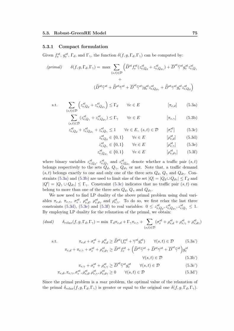
5.3. Robust-GreenRE Model 75
5.3.1 Compact formulation
Given fste , gste , Γd, and Γγ , the function δ(f, g,Γd,Γγ) can be computed by:
(primal) δ(f, g,Γd,Γγ) = max∑
(s,t)∈D
(Dstfste (zste,Qd + zste,Qdγ ) +D
stγstgste z
ste,Qγ
+
(Dstγst + Dstγst +Dstγst)gste z
ste,Qdγ
+ Dstγstgste zste,Qd
)
s.t.∑
(s,t)∈D
(zste,Qd + zste,Qdγ
)≤ Γd ∀e ∈ E [πe,d] (5.3a)
∑(s,t)∈D
(zste,Qγ + zste,Qdγ ) ≤ Γγ ∀e ∈ E [πe,γ ] (5.3b)
zste,Qd + zste,Qdγ + zste,Qγ ≤ 1 ∀e ∈ E, (s, t) ∈ D [σste ] (5.3c)
zste,Qd ∈ {0, 1} ∀e ∈ E [ρste,d] (5.3d)
zste,Qγ ∈ {0, 1} ∀e ∈ E [ρste,γ ] (5.3e)
zste,Qdγ ∈ {0, 1} ∀e ∈ E [ρste,dγ ] (5.3f)
where binary variables zste,Qd , zste,Qγ
and zste,Qdγ denote whether a traffic pair (s, t)
belongs respectively to the sets Qd, Qγ , Qdγ or not. Note that, a traffic demand(s, t) belongs exactly to one and only one of the three sets Qd, Qγ and Qdγ . Con-straints (5.3a) and (5.3b) are used to limit size of the set |Q| = |Qd∪Qdγ | ≤ Γd and|Q′| = |Qγ ∪ Qdγ | ≤ Γγ . Constraint (5.3c) indicates that no traffic pair (s, t) canbelong to more than one of the three sets Qd, Qγ and Qdγ .
We now need to find LP duality of the above primal problem using dual vari-ables πe,d, πe,γ , σste , ρste,d, ρ
ste,dγ and ρste,γ . To do so, we first relax the last three
constraints (5.3d), (5.3e) and (5.3f) to real variables: 0 ≤ zste,Qd , zste,Qdγ
, zste,Qγ ≤ 1.By employing LP duality for the relaxation of the primal, we obtain:
(dual) δrelax(f, g,Γd,Γγ) = min Γdπe,d + Γγπe,γ +∑
(s,t)∈D
(σste + ρste,d + ρste,γ + ρste,dγ)
s.t. πe,d + σste + ρste,d ≥ Dst(f ste + γstgste ) ∀(s, t) ∈ D (5.3a’)
πe,d + πe,γ + σste + ρste,dγ ≥ Dstfste +(Dstγst + Dstγst +D
stγst)gste
∀(s, t) ∈ D (5.3b’)
πe,γ + σste + ρste,γ ≥ Dstγstgste ∀(s, t) ∈ D (5.3c’)
πe,d, πe,γ , σste , ρ
ste,d, ρ
ste,γ , ρ
ste,dγ ≥ 0 ∀(s, t) ∈ D (5.3d’)
Since the primal problem is a max problem, the optimal value of the relaxation ofthe primal δrelax(f, g,Γd,Γγ) is greater or equal to the original one δ(f, g,Γd,Γγ).
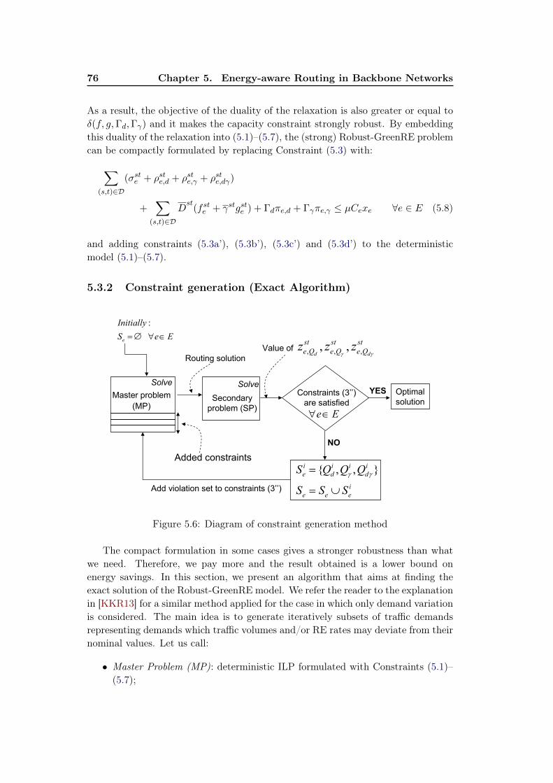
76 Chapter 5. Energy-aware Routing in Backbone Networks
As a result, the objective of the duality of the relaxation is also greater or equal toδ(f, g,Γd,Γγ) and it makes the capacity constraint strongly robust. By embeddingthis duality of the relaxation into (5.1)–(5.7), the (strong) Robust-GreenRE problemcan be compactly formulated by replacing Constraint (5.3) with:∑
(s,t)∈D
(σste + ρste,d + ρste,γ + ρste,dγ)
+∑
(s,t)∈D
Dst
(fste + γstgste ) + Γdπe,d + Γγπe,γ ≤ µCexe ∀e ∈ E (5.8)
and adding constraints (5.3a’), (5.3b’), (5.3c’) and (5.3d’) to the deterministicmodel (5.1)–(5.7).
5.3.2 Constraint generation (Exact Algorithm)
Master problem
(MP)
Routing solution
Add violation set to constraints (3’’)
Solve
:
e
Initially
S e E=∅ ∀ ∈
e E∀ ∈
Secondary
problem (SP)
Solve
Constraints (3’’)
are satisfied
, , ,, ,d d
st st st
e Q e Q e Qz z zγ γ
Value of
Optimal
solution
YES
{ , , }i i i i
e d d
i
e e e
S Q Q Q
S S S
γ γ=
= ∪
Added constraints
NO
Figure 5.6: Diagram of constraint generation method
The compact formulation in some cases gives a stronger robustness than whatwe need. Therefore, we pay more and the result obtained is a lower bound onenergy savings. In this section, we present an algorithm that aims at finding theexact solution of the Robust-GreenRE model. We refer the reader to the explanationin [KKR13] for a similar method applied for the case in which only demand variationis considered. The main idea is to generate iteratively subsets of traffic demandsrepresenting demands which traffic volumes and/or RE rates may deviate from theirnominal values. Let us call:
• Master Problem (MP): deterministic ILP formulated with Constraints (5.1)–(5.7);
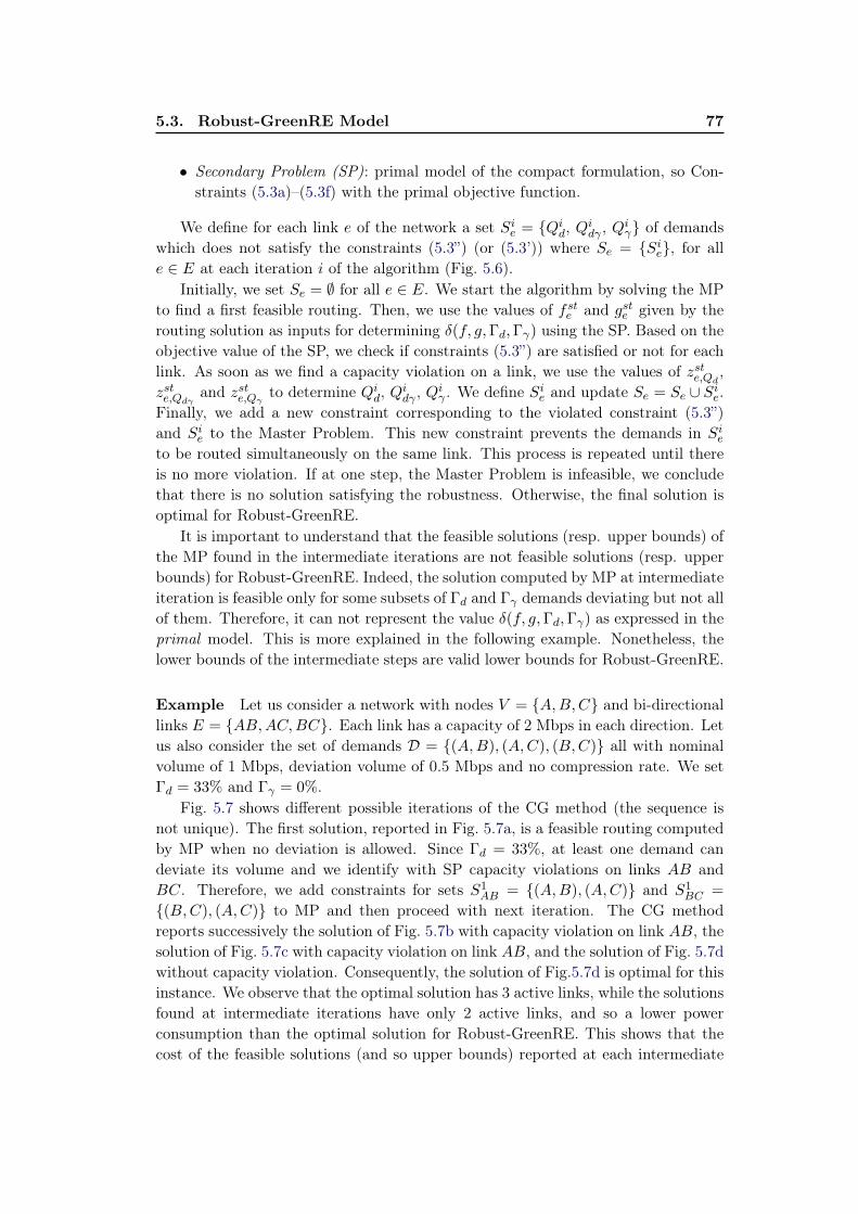
5.3. Robust-GreenRE Model 77
• Secondary Problem (SP): primal model of the compact formulation, so Con-straints (5.3a)–(5.3f) with the primal objective function.
We define for each link e of the network a set Sie = {Qid, Qidγ , Qiγ} of demandswhich does not satisfy the constraints (5.3”) (or (5.3’)) where Se = {Sie}, for alle ∈ E at each iteration i of the algorithm (Fig. 5.6).
Initially, we set Se = ∅ for all e ∈ E. We start the algorithm by solving the MPto find a first feasible routing. Then, we use the values of fste and gste given by therouting solution as inputs for determining δ(f, g,Γd,Γγ) using the SP. Based on theobjective value of the SP, we check if constraints (5.3”) are satisfied or not for eachlink. As soon as we find a capacity violation on a link, we use the values of zste,Qd ,zste,Qdγ and zste,Qγ to determine Qid, Q
idγ , Q
iγ . We define Sie and update Se = Se ∪ Sie.
Finally, we add a new constraint corresponding to the violated constraint (5.3”)and Sie to the Master Problem. This new constraint prevents the demands in Sieto be routed simultaneously on the same link. This process is repeated until thereis no more violation. If at one step, the Master Problem is infeasible, we concludethat there is no solution satisfying the robustness. Otherwise, the final solution isoptimal for Robust-GreenRE.
It is important to understand that the feasible solutions (resp. upper bounds) ofthe MP found in the intermediate iterations are not feasible solutions (resp. upperbounds) for Robust-GreenRE. Indeed, the solution computed by MP at intermediateiteration is feasible only for some subsets of Γd and Γγ demands deviating but not allof them. Therefore, it can not represent the value δ(f, g,Γd,Γγ) as expressed in theprimal model. This is more explained in the following example. Nonetheless, thelower bounds of the intermediate steps are valid lower bounds for Robust-GreenRE.
Example Let us consider a network with nodes V = {A,B,C} and bi-directionallinks E = {AB,AC,BC}. Each link has a capacity of 2 Mbps in each direction. Letus also consider the set of demands D = {(A,B), (A,C), (B,C)} all with nominalvolume of 1 Mbps, deviation volume of 0.5 Mbps and no compression rate. We setΓd = 33% and Γγ = 0%.
Fig. 5.7 shows different possible iterations of the CG method (the sequence isnot unique). The first solution, reported in Fig. 5.7a, is a feasible routing computedby MP when no deviation is allowed. Since Γd = 33%, at least one demand candeviate its volume and we identify with SP capacity violations on links AB andBC. Therefore, we add constraints for sets S1
AB = {(A,B), (A,C)} and S1BC =
{(B,C), (A,C)} to MP and then proceed with next iteration. The CG methodreports successively the solution of Fig. 5.7b with capacity violation on link AB, thesolution of Fig. 5.7c with capacity violation on link AB, and the solution of Fig. 5.7dwithout capacity violation. Consequently, the solution of Fig.5.7d is optimal for thisinstance. We observe that the optimal solution has 3 active links, while the solutionsfound at intermediate iterations have only 2 active links, and so a lower powerconsumption than the optimal solution for Robust-GreenRE. This shows that thecost of the feasible solutions (and so upper bounds) reported at each intermediate
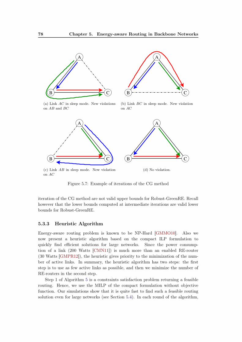
78 Chapter 5. Energy-aware Routing in Backbone Networks
A
B C
(a) Link AC in sleep mode. New violationson AB and BC
A
B C
(b) Link BC in sleep mode. New violationon AC
A
B C
(c) Link AB in sleep mode. New violationon AC
A
B C
(d) No violation.
Figure 5.7: Example of iterations of the CG method
iteration of the CG method are not valid upper bounds for Robust-GreenRE. Recallhowever that the lower bounds computed at intermediate iterations are valid lowerbounds for Robust-GreenRE.
5.3.3 Heuristic Algorithm
Energy-aware routing problem is known to be NP-Hard [GMMO10]. Also wenow present a heuristic algorithm based on the compact ILP formulation toquickly find efficient solutions for large networks. Since the power consump-tion of a link (200 Watts [CMN11]) is much more than an enabled RE-router(30 Watts [GMPR12]), the heuristic gives priority to the minimization of the num-ber of active links. In summary, the heuristic algorithm has two steps: the firststep is to use as few active links as possible, and then we minimize the number ofRE-routers in the second step.
Step 1 of Algorithm 5 is a constraints satisfaction problem returning a feasiblerouting. Hence, we use the MILP of the compact formulation without objectivefunction. Our simulations show that it is quite fast to find such a feasible routingsolution even for large networks (see Section 5.4). In each round of the algorithm,
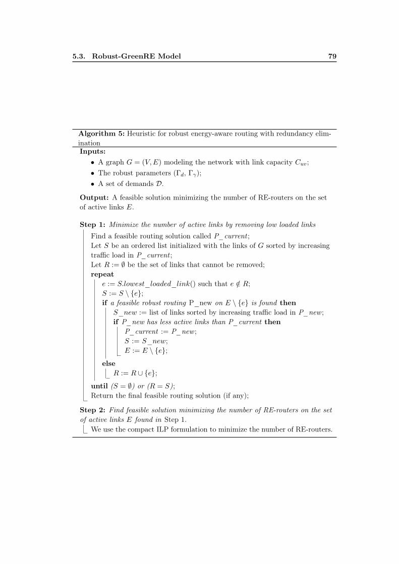
5.3. Robust-GreenRE Model 79
Algorithm 5: Heuristic for robust energy-aware routing with redundancy elim-inationInputs:• A graph G = (V,E) modeling the network with link capacity Cuv;• The robust parameters (Γd, Γγ);• A set of demands D.
Output: A feasible solution minimizing the number of RE-routers on the setof active links E.
Step 1: Minimize the number of active links by removing low loaded linksFind a feasible routing solution called P_current ;Let S be an ordered list initialized with the links of G sorted by increasingtraffic load in P_current ;Let R := ∅ be the set of links that cannot be removed;repeat
e := S.lowest_loaded_link() such that e /∈ R;S := S \ {e};if a feasible robust routing P_new on E \ {e} is found then
S_new := list of links sorted by increasing traffic load in P_new ;if P_new has less active links than P_current then
P_current := P_new ;S := S_new;E := E \ {e};
elseR := R ∪ {e};
until (S = ∅) or (R = S);Return the final feasible routing solution (if any);
Step 2: Find feasible solution minimizing the number of RE-routers on the setof active links E found in Step 1.
We use the compact ILP formulation to minimize the number of RE-routers.
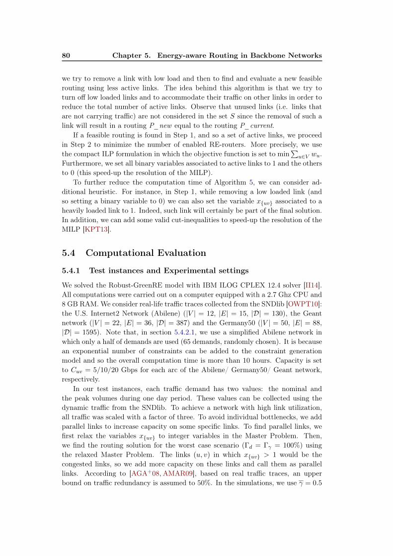
80 Chapter 5. Energy-aware Routing in Backbone Networks
we try to remove a link with low load and then to find and evaluate a new feasiblerouting using less active links. The idea behind this algorithm is that we try toturn off low loaded links and to accommodate their traffic on other links in order toreduce the total number of active links. Observe that unused links (i.e. links thatare not carrying traffic) are not considered in the set S since the removal of such alink will result in a routing P_new equal to the routing P_current.
If a feasible routing is found in Step 1, and so a set of active links, we proceedin Step 2 to minimize the number of enabled RE-routers. More precisely, we usethe compact ILP formulation in which the objective function is set to min
∑u∈V wu.
Furthermore, we set all binary variables associated to active links to 1 and the othersto 0 (this speed-up the resolution of the MILP).
To further reduce the computation time of Algorithm 5, we can consider ad-ditional heuristic. For instance, in Step 1, while removing a low loaded link (andso setting a binary variable to 0) we can also set the variable x{uv} associated to aheavily loaded link to 1. Indeed, such link will certainly be part of the final solution.In addition, we can add some valid cut-inequalities to speed-up the resolution of theMILP [KPT13].
5.4 Computational Evaluation
5.4.1 Test instances and Experimental settings
We solved the Robust-GreenRE model with IBM ILOG CPLEX 12.4 solver [II14].All computations were carried out on a computer equipped with a 2.7 Ghz CPU and8 GB RAM. We consider real-life traffic traces collected from the SNDlib [OWPT10]:the U.S. Internet2 Network (Abilene) (|V | = 12, |E| = 15, |D| = 130), the Geantnetwork (|V | = 22, |E| = 36, |D| = 387) and the Germany50 (|V | = 50, |E| = 88,|D| = 1595). Note that, in section 5.4.2.1, we use a simplified Abilene network inwhich only a half of demands are used (65 demands, randomly chosen). It is becausean exponential number of constraints can be added to the constraint generationmodel and so the overall computation time is more than 10 hours. Capacity is setto Cuv = 5/10/20 Gbps for each arc of the Abilene/ Germany50/ Geant network,respectively.
In our test instances, each traffic demand has two values: the nominal andthe peak volumes during one day period. These values can be collected using thedynamic traffic from the SNDlib. To achieve a network with high link utilization,all traffic was scaled with a factor of three. To avoid individual bottlenecks, we addparallel links to increase capacity on some specific links. To find parallel links, wefirst relax the variables x{uv} to integer variables in the Master Problem. Then,we find the routing solution for the worst case scenario (Γd = Γγ = 100%) usingthe relaxed Master Problem. The links (u, v) in which x{uv} > 1 would be thecongested links, so we add more capacity on these links and call them as parallellinks. According to [AGA+08, AMAR09], based on real traffic traces, an upperbound on traffic redundancy is assumed to 50%. In the simulations, we use γ = 0.5
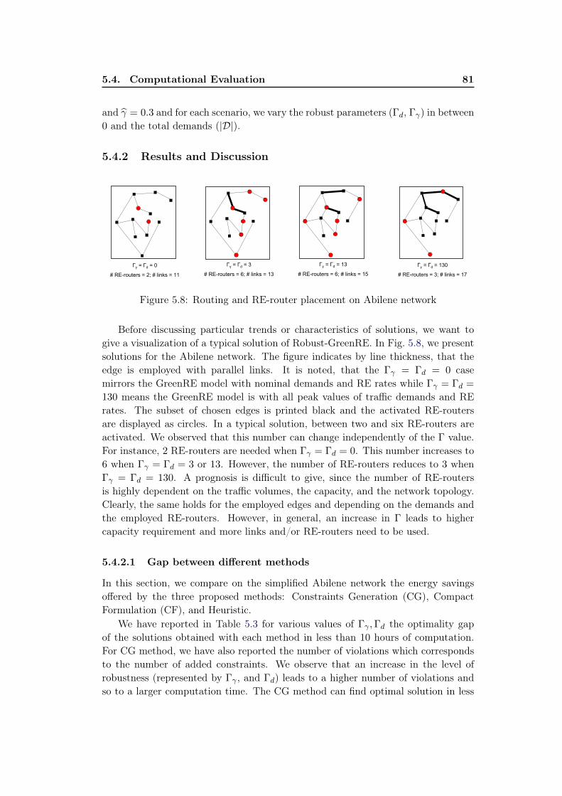
5.4. Computational Evaluation 81
and γ = 0.3 and for each scenario, we vary the robust parameters (Γd, Γγ) in between0 and the total demands (|D|).
5.4.2 Results and Discussion
Гγ = Гd = 130
# RE-routers = 3; # links = 17
Гγ = Гd = 0
# RE-routers = 2; # links = 11
Гγ = Гd = 3
# RE-routers = 6; # links = 13
Гγ = Гd = 13
# RE-routers = 6; # links = 15
Figure 5.8: Routing and RE-router placement on Abilene network
Before discussing particular trends or characteristics of solutions, we want togive a visualization of a typical solution of Robust-GreenRE. In Fig. 5.8, we presentsolutions for the Abilene network. The figure indicates by line thickness, that theedge is employed with parallel links. It is noted, that the Γγ = Γd = 0 casemirrors the GreenRE model with nominal demands and RE rates while Γγ = Γd =
130 means the GreenRE model is with all peak values of traffic demands and RErates. The subset of chosen edges is printed black and the activated RE-routersare displayed as circles. In a typical solution, between two and six RE-routers areactivated. We observed that this number can change independently of the Γ value.For instance, 2 RE-routers are needed when Γγ = Γd = 0. This number increases to6 when Γγ = Γd = 3 or 13. However, the number of RE-routers reduces to 3 whenΓγ = Γd = 130. A prognosis is difficult to give, since the number of RE-routersis highly dependent on the traffic volumes, the capacity, and the network topology.Clearly, the same holds for the employed edges and depending on the demands andthe employed RE-routers. However, in general, an increase in Γ leads to highercapacity requirement and more links and/or RE-routers need to be used.
5.4.2.1 Gap between different methods
In this section, we compare on the simplified Abilene network the energy savingsoffered by the three proposed methods: Constraints Generation (CG), CompactFormulation (CF), and Heuristic.
We have reported in Table 5.3 for various values of Γγ ,Γd the optimality gapof the solutions obtained with each method in less than 10 hours of computation.For CG method, we have also reported the number of violations which correspondsto the number of added constraints. We observe that an increase in the level ofrobustness (represented by Γγ , and Γd) leads to a higher number of violations andso to a larger computation time. The CG method can find optimal solution in less
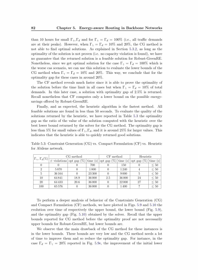
82 Chapter 5. Energy-aware Routing in Backbone Networks
than 10 hours for small Γγ ,Γd and for Γγ = Γd = 100% (i.e., all traffic demandsare at their peaks). However, when Γγ = Γd = 10% and 20%, the CG method isnot able to find optimal solutions. As explained in Section 5.3.2, as long as theoptimality of the solution is not proven (i.e. no capacity violation is found), we haveno guarantee that the returned solution is a feasible solution for Robust-GreenRE.Nonetheless, since we get optimal solution for the case Γγ = Γd = 100% which isthe worse cas scenario, we can use this solution to evaluate the lower bounds of theCG method when Γγ = Γd = 10% and 20%. This way, we conclude that for theoptimality gap for these cases in around 20%.
The CF method reveals much faster since it is able to prove the optimality ofthe solution before the time limit in all cases but when Γγ = Γd = 10% of totaldemands. In this later case, a solution with optimality gap of 2.5% is returned.Recall nonetheless that CF computes only a lower bound on the possible energy-savings offered by Robust-GreenRE.
Finally, and as expected, the heuristic algorithm is the fastest method. Allfeasible solutions are found in less than 50 seconds. To evaluate the quality of thesolutions returned by the heuristic, we have reported in Table 5.3 the optimalitygap as the ratio of the value of the solution computed with the heuristic over thebest lower bound returned by the solver for the CG method. The optimality gap isless than 5% for small values of Γγ ,Γd, and it is around 25% for larger values. Thisindicates that the heuristic is able to quickly returned good solutions.
Table 5.3: Constraint Generation (CG) vs. Compact Formulation (CF) vs. Heuristicfor Abilene network.
Γγ , Γd(%)CG method CF method Heuristic
# violations opt gap (%) time (s) opt gap (%) time (s) opt gap (%) time (s)0 0 0 700 0 150 0 ≤ 502 5 870 0 1 800 0 1 240 4 ≤ 505 36 164 0 23 300 0 9 000 5 ≤ 5010 64 841 18.9 36 000 2.5 36 000 24 ≤ 5020 64 433 20.6 36 000 0 22 000 27 ≤ 50100 65 576 0 36 000 0 1 400 7 ≤ 50
To perform a deeper analysis of behavior of the Constraints Generation (CG)and Compact Formulation (CF) methods, we have plotted in Figs. 5.9 and 5.10 theevolution over time of respectively the upper bound, the lower bound (Fig. 5.9),and the optimality gap (Fig. 5.10) obtained by the solver. Recall that the upperbounds reported for CG method before the optimality proof are not necessarilyupper bounds for Robust-GreenRE, but lower bounds are.
We observe that the main drawback of the CG method for these instances isin the lower bounds. These bounds are very low and the CG method needs a lotof time to improve them and so reduce the optimality gap. For instance, in thecase Γd = Γγ = 20% reported in Fig. 5.9e, the improvement of the initial lower
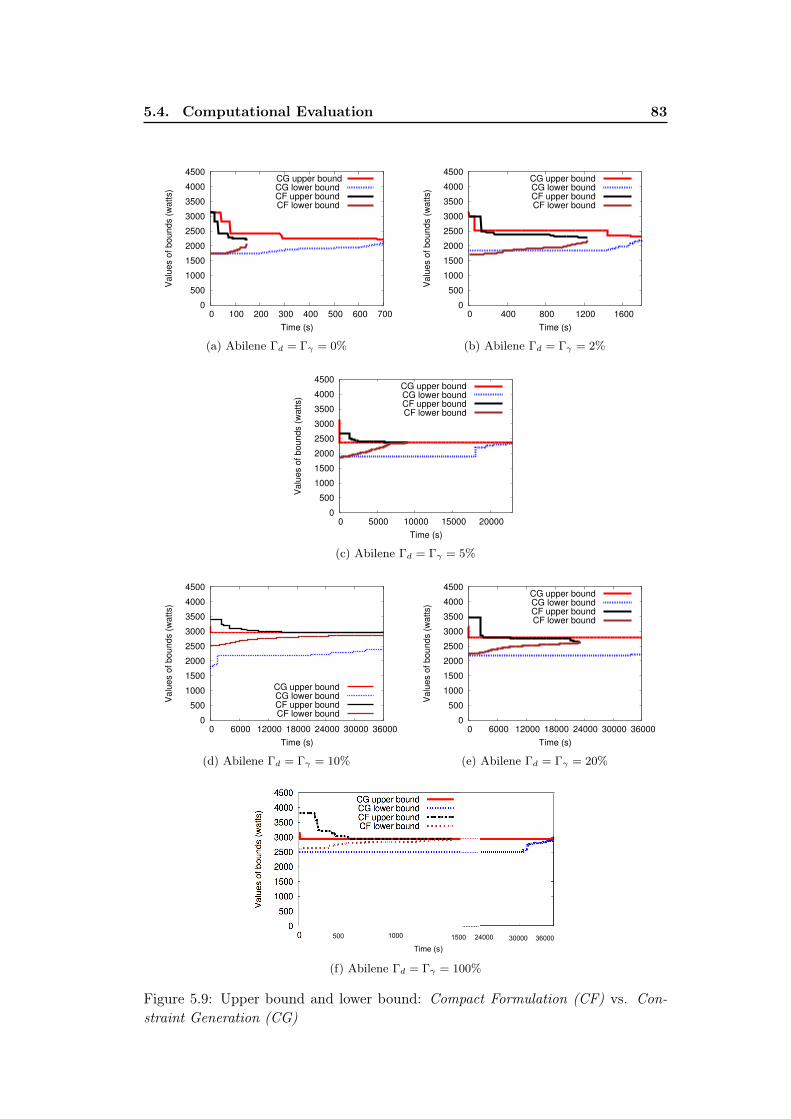
5.4. Computational Evaluation 83
0
500
1000
1500
2000
2500
3000
3500
4000
4500
0 100 200 300 400 500 600 700
Val
ues
of b
ound
s (w
atts
)
Time (s)
CG upper boundCG lower bound CF upper bound CF lower bound
(a) Abilene Γd = Γγ = 0%
0
500
1000
1500
2000
2500
3000
3500
4000
4500
0 400 800 1200 1600
Val
ues
of b
ound
s (w
atts
)
Time (s)
CG upper bound CG lower bound CF upper bound CF lower bound
(b) Abilene Γd = Γγ = 2%
0
500
1000
1500
2000
2500
3000
3500
4000
4500
0 5000 10000 15000 20000
Val
ues
of b
ound
s (w
atts
)
Time (s)
CG upper bound CG lower bound CF upper bound CF lower bound
(c) Abilene Γd = Γγ = 5%
0
500
1000
1500
2000
2500
3000
3500
4000
4500
0 6000 12000 18000 24000 30000 36000
Val
ues
of b
ound
s (w
atts
)
Time (s)
CG upper bound CG lower bound CF upper bound CF lower bound
(d) Abilene Γd = Γγ = 10%
0
500
1000
1500
2000
2500
3000
3500
4000
4500
0 6000 12000 18000 24000 30000 36000
Val
ues
of b
ound
s (w
atts
)
Time (s)
CG upper bound CG lower bound CF upper bound CF lower bound
(e) Abilene Γd = Γγ = 20%
1500500 1000 24000 30000 36000
Time (s)
(f) Abilene Γd = Γγ = 100%
Figure 5.9: Upper bound and lower bound: Compact Formulation (CF) vs. Con-straint Generation (CG)
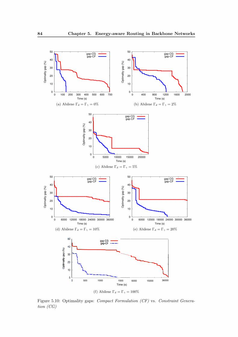
84 Chapter 5. Energy-aware Routing in Backbone Networks
0
10
20
30
40
50
0 100 200 300 400 500 600 700
Opt
imal
ity g
ap (%
)
Time (s)
gap-CG gap-CF
(a) Abilene Γd = Γγ = 0%
0
10
20
30
40
50
0 400 800 1200 1600 2000
Opt
imal
ity g
ap (%
)
Time (s)
gap-CG gap-CF
(b) Abilene Γd = Γγ = 2%
0
10
20
30
40
50
0 5000 10000 15000 20000
Opt
imal
ity g
ap (%
)
Time (s)
gap-CG gap-CF
(c) Abilene Γd = Γγ = 5%
0
10
20
30
40
50
0 6000 12000 18000 24000 30000 36000
Opt
imal
ity g
ap (%
)
Time (s)
gap-CG gap-CF
(d) Abilene Γd = Γγ = 10%
0
10
20
30
40
50
0 6000 12000 18000 24000 30000 36000
Opt
imal
ity g
ap (%
)
Time (s)
gap-CG gap-CF
(e) Abilene Γd = Γγ = 20%
1500500 1000
Time (s)
6000 3600015000
(f) Abilene Γd = Γγ = 100%
Figure 5.10: Optimality gaps: Compact Formulation (CF) vs. Constraint Genera-tion (CG)
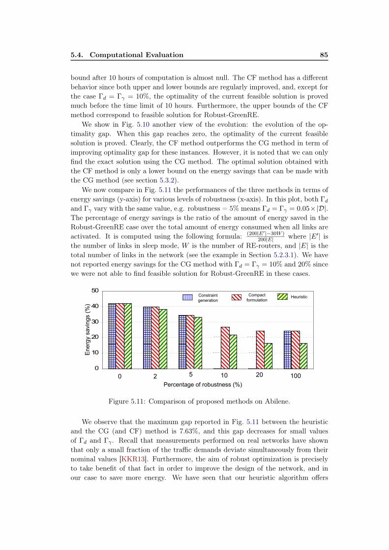
5.4. Computational Evaluation 85
bound after 10 hours of computation is almost null. The CF method has a differentbehavior since both upper and lower bounds are regularly improved, and, except forthe case Γd = Γγ = 10%, the optimality of the current feasible solution is provedmuch before the time limit of 10 hours. Furthermore, the upper bounds of the CFmethod correspond to feasible solution for Robust-GreenRE.
We show in Fig. 5.10 another view of the evolution: the evolution of the op-timality gap. When this gap reaches zero, the optimality of the current feasiblesolution is proved. Clearly, the CF method outperforms the CG method in term ofimproving optimality gap for these instances. However, it is noted that we can onlyfind the exact solution using the CG method. The optimal solution obtained withthe CF method is only a lower bound on the energy savings that can be made withthe CG method (see section 5.3.2).
We now compare in Fig. 5.11 the performances of the three methods in terms ofenergy savings (y-axis) for various levels of robustness (x-axis). In this plot, both Γdand Γγ vary with the same value, e.g. robustness = 5% means Γd = Γγ = 0.05×|D|.The percentage of energy savings is the ratio of the amount of energy saved in theRobust-GreenRE case over the total amount of energy consumed when all links areactivated. It is computed using the following formula: (200|E′|−30W )
200|E| where |E′| isthe number of links in sleep mode, W is the number of RE-routers, and |E| is thetotal number of links in the network (see the example in Section 5.2.3.1). We havenot reported energy savings for the CG method with Γd = Γγ = 10% and 20% sincewe were not able to find feasible solution for Robust-GreenRE in these cases.
0
10
20
30
40
50
1 2 3 4 5 6
Energ
y s
avin
gs (
%)
2 5 10 20
Constraint
generationHeuristicCompact
formulation
Percentage of robustness (%)
1000
Figure 5.11: Comparison of proposed methods on Abilene.
We observe that the maximum gap reported in Fig. 5.11 between the heuristicand the CG (and CF) method is 7.63%, and this gap decreases for small valuesof Γd and Γγ . Recall that measurements performed on real networks have shownthat only a small fraction of the traffic demands deviate simultaneously from theirnominal values [KKR13]. Furthermore, the aim of robust optimization is preciselyto take benefit of that fact in order to improve the design of the network, and inour case to save more energy. We have seen that our heuristic algorithm offers
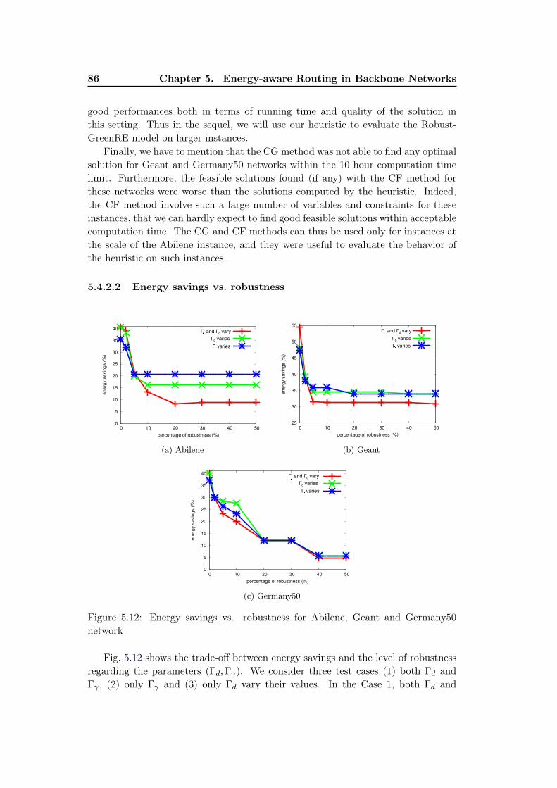
86 Chapter 5. Energy-aware Routing in Backbone Networks
good performances both in terms of running time and quality of the solution inthis setting. Thus in the sequel, we will use our heuristic to evaluate the Robust-GreenRE model on larger instances.
Finally, we have to mention that the CG method was not able to find any optimalsolution for Geant and Germany50 networks within the 10 hour computation timelimit. Furthermore, the feasible solutions found (if any) with the CF method forthese networks were worse than the solutions computed by the heuristic. Indeed,the CF method involve such a large number of variables and constraints for theseinstances, that we can hardly expect to find good feasible solutions within acceptablecomputation time. The CG and CF methods can thus be used only for instances atthe scale of the Abilene instance, and they were useful to evaluate the behavior ofthe heuristic on such instances.
5.4.2.2 Energy savings vs. robustness
0
5
10
15
20
25
30
35
40
0 10 20 30 40 50
ener
gy s
avin
gs (%
)
percentage of robustness (%)
1
2
3
Гd varies
Г varies
Г and Гd vary
(a) Abilene
25
30
35
40
45
50
55
0 10 20 30 40 50
ener
gy s
avin
gs (%
)
percentage of robustness (%)
1
2
3
Г and Гd vary
Гd varies
Г varies
(b) Geant
0
5
10
15
20
25
30
35
40
0 10 20 30 40 50
ener
gy s
avin
gs (%
)
percentage of robustness (%)
1
2
3
Г and Гd vary
Гd varies
Г varies
(c) Germany50
Figure 5.12: Energy savings vs. robustness for Abilene, Geant and Germany50network
Fig. 5.12 shows the trade-off between energy savings and the level of robustnessregarding the parameters (Γd,Γγ). We consider three test cases (1) both Γd andΓγ , (2) only Γγ and (3) only Γd vary their values. In the Case 1, both Γd and
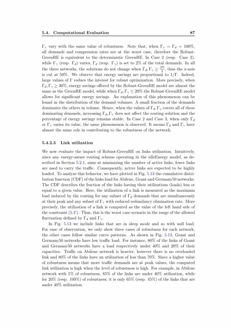
5.4. Computational Evaluation 87
Γγ vary with the same value of robustness. Note that, when Γγ = Γd = 100%,all demands and compression rates are at the worst case, therefore the Robust-GreenRE is equivalent to the deterministic GreenRE. In Case 2 (resp. Case 3),while Γγ (resp. Γd) varies, Γd (resp. Γγ) is set to 2% of the total demands. In allthe three networks, the solutions do not change when Γd,Γγ ≥ |D|2 , thus the x-axisis cut at 50%. We observe that energy savings are proportional to 1/Γ. Indeed,large values of Γ reduce the interest for robust optimization. More precisely, whenΓd,Γγ ≥ 30%, energy savings offered by the Robust-GreenRE model are almost thesame as the GreenRE model, while when Γd,Γγ ≤ 20% the Robust-GreenRE modelallows for significant energy savings. An explanation of this phenomenon can befound in the distribution of the demand volumes. A small fraction of the demandsdominates the others in volume. Hence, when the values of Γd,Γγ covers all of thesedominating demands, increasing Γd,Γγ does not affect the routing solution and thepercentage of energy savings remains stable. In Case 2 and Case 3, when only Γdor Γγ varies its value, the same phenomenon is observed. It means Γd and Γγ havealmost the same role in contributing to the robustness of the network.
5.4.2.3 Link utilization
We now evaluate the impact of Robust-GreenRE on links utilization. Intuitively,since any energy-aware routing scheme operating in the idleEnergy model, as de-scribed in Section 5.2.1, aims at minimizing the number of active links, fewer linksare used to carry the traffic. Consequently, active links are expected to be highlyloaded. To analyze this behavior, we have plotted in Fig. 5.13 the cumulative distri-bution function (CDF) of the links load for Abilene, Geant and Germany50 networks.The CDF describes the fraction of the links having their utilizations (loads) less orequal to a given value. Here, the utilization of a link is measured as the maximumload induced by the routing for any subset of Γd demands that are simultaneouslyat their peak and any subset of Γγ with reduced redundancy elimination rate. Moreprecisely, the utilization of a link is computed as the value of the left hand side ofthe constraint (5.3’). Thus, this is the worst case scenario in the range of the allowedfluctuation defined by Γd and Γγ .
In Fig. 5.13 we include links that are in sleep mode and so with null load.For ease of observation, we only show three cases of robustness for each network,the other cases follow similar curve patterns. As shown in Fig. 5.13, Geant andGermany50 networks have low traffic load. For instance, 80% of the links of Geantand Germany50 networks have a load respectively under 40% and 20% of theircapacities. Traffic on Abilene network is heavier, however there is no overloadedlink and 80% of the links have an utilization of less than 70%. Since a higher valueof robustness means that more traffic demands are at peak values, the computedlink utilization is high when the level of robustness is high. For example, in Abilenenetwork with 5% of robustness, 85% of the links are under 40% utilization, whilefor 20% (resp. 100%) of robustness, it is only 65% (resp. 45%) of the links that areunder 40% utilization.
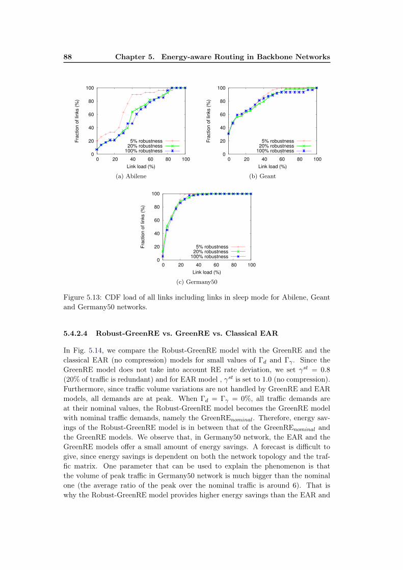
88 Chapter 5. Energy-aware Routing in Backbone Networks
0
20
40
60
80
100
0 20 40 60 80 100
Frac
tion
of li
nks
(%)
Link load (%)
5% robustness20% robustness
100% robustness
(a) Abilene
0
20
40
60
80
100
0 20 40 60 80 100
Frac
tion
of li
nks
(%)
Link load (%)
5% robustness20% robustness
100% robustness
(b) Geant
0
20
40
60
80
100
0 20 40 60 80 100
Frac
tion
of li
nks
(%)
Link load (%)
5% robustness20% robustness
100% robustness
(c) Germany50
Figure 5.13: CDF load of all links including links in sleep mode for Abilene, Geantand Germany50 networks.
5.4.2.4 Robust-GreenRE vs. GreenRE vs. Classical EAR
In Fig. 5.14, we compare the Robust-GreenRE model with the GreenRE and theclassical EAR (no compression) models for small values of Γd and Γγ . Since theGreenRE model does not take into account RE rate deviation, we set γst = 0.8
(20% of traffic is redundant) and for EAR model , γst is set to 1.0 (no compression).Furthermore, since traffic volume variations are not handled by GreenRE and EARmodels, all demands are at peak. When Γd = Γγ = 0%, all traffic demands areat their nominal values, the Robust-GreenRE model becomes the GreenRE modelwith nominal traffic demands, namely the GreenREnominal. Therefore, energy sav-ings of the Robust-GreenRE model is in between that of the GreenREnominal andthe GreenRE models. We observe that, in Germany50 network, the EAR and theGreenRE models offer a small amount of energy savings. A forecast is difficult togive, since energy savings is dependent on both the network topology and the traf-fic matrix. One parameter that can be used to explain the phenomenon is thatthe volume of peak traffic in Germany50 network is much bigger than the nominalone (the average ratio of the peak over the nominal traffic is around 6). That iswhy the Robust-GreenRE model provides higher energy savings than the EAR and
5.5. Conclusion 89
0
10
20
30
40
50
60
70
1 2 3
En
erg
y s
avin
gs (
%)
Network topologies
Abilene Geant Germany50
Гd = Гγ = 0% Гd = Гγ = 2%Гd = 2%
Гγ = 5%
Гd = 5%
Гγ = 2%GreenRE EAR
Figure 5.14: Robust-GreenRE vs. GreenRE vs. EAR.
the GreenRE model in Germany50 network. It is noted that the Robust-GreenREmodel is more efficient than the GreenRE model when only few traffic demandsfluctuate their volumes and RE rates (Γ is relatively small). When Γ is quite big,e.g. Γ >= 20%, the Robust-GreenRE and the GreenRE models yield almost thesame amount of energy saving (as shown in Fig. 5.12). However, this result does notinvalidate the benefit of Γ-robustness because in real-life traffic, only a few demandswill vary their traffic simultaneously [KKR13]. In summary, when Γ = 2 − 5%,the Robust-GreenRE model outperforms the other models and allows for 16− 28%
additional energy savings in all the considered networks.
5.5 Conclusion
In this work, we have formally defined and modeled the Robust-GreenRE problemand applyied it to backbone networks. Taking into account the uncertainties oftraffic volumes and redundancy elimination rates, the Robust-GreenRE model pro-vides a more accurate evaluation of energy savings for backbone networks. Basedon real-life traffic traces, we have shown a significant improvement of energy savingscompared with other models. As future work, we shall investigate implementationissues and impacts of Robust-GreenRE model on QoS and fault tolerance. We shallalso look into other available methods that together with EAR, could be directlyapplied to wireless backhaul networks.

Chapter 6
Conclusion
With the increasing demand of data bandwidth, high-speed and reliable services bymobile subscribers and with the improvements in the access networks, the capacitybottleneck of cellular networks has moved toward the backhaul. In this thesis,we have studied several optimization problems related to the minimization of theCAPEX and OPEX of backhaul networks, and on the improvement of the revenuesof the network operator.
In Chapter 3, we studied the problem of dimensioning a fixed broadband wirelessnetwork under unreliable conditions. It consists in assigning bandwidth, thus capac-ity, to the links in order to minimize the annual fees of renting the bandwidth whileall the demands are satisfied with high probability. In our formulation, we consid-ered a dynamic routing approach of demands and we proposed a column generationalgorithm to solve the problem. To assess our method, we have performed numer-ical evaluation on realistic network instances. Our results show that our approachallows for up to 45% of cost savings regarding to the worst case. A comparisonof our results with those of previous work validates the efficiency of our solution,specifically on large instances.
In Chapter 4, we applied the infrastructure sharing concept to backhaul net-works, that is highly recommanded by regulatory authorithies. The goal was tohelp the owner of the network infrastructure to increase its income by renting itsnetwork to other operators. We thus investigate the problem of maximizing the totalrenting revenue of the PNO in a multi-operator network context and under demanduncertainties and QoS requirements. We formally defined a Γ-robust Mixed IntegerLinear Program (MILP) to model the problem, and we evaluated our formulationon several real-life network topologies. In particular, we analyzed the impact of therobustness level and that of the agreed SLA on the PNO revenue. However, ourILP formulation is hard to solve on large-scale networks. Also, we proposed differ-ent heuristics to find efficient solutions in lower resolution time. Our experimentsshowed the computation time reductions offered by the greedy and the powersetheuristics with almost the same solutions quality.
Besides, we worked on the green networking field, more specifically we investi-gated the problem of reducing the energy consumption of backbone networks. Wecombined the strengths of energy-aware routing (EAR) with the concept of datatraffic redundancy elimination (RE) to maximize the energy saving in the contextof variable demand volumes and RE rates. We formalized the problem as a MILPusing Γ-robustness method. We proposed three different resolution methods for this
92 Chapter 6. Conclusion
NP-hard problem. The simulation results on different network instances highlightedan extra energy savings from 16% to 28% with respect to the simple EAR model.
In this thesis, we have investigated some open questions related to the opti-mization and the cost-effectiveness of microwave backhaul networks. Nonetheless,many questions remain open. For instance, further algorithmic improvements areneeded for the resolution of the problem of dimensioning a fixed broadband wirelessnetworks under unreliable conditions, in particular to speed up the exploration ofthe feasibility set of the pricing problem and improve the reliability of the solutions.Another research direction is to introduce in this design problem some correlationbetween microwave links configurations. More precisely, environmental conditionsmay affect simultaneously geographically localized links. For instance, a storm willaffect the radio propagation of all links incident to a particular node of the network.The inclusion of such correlation into the design problem may lead to another ex-pression of a network scenario probability, and help to propose a more realisticsolution to this problem.
Another interesting question is related to the long term deployment and im-provement of backhaul networks. Typically, the network operator needs accuraterecommandations on where and when to invest for either adding new microwavelinks (densification or coverage extension), or to connect to a neighboring opticalnetwork, or to install a new optical link, or even to stop using a link that is no longeruseful. This raised many challenging questions that are hard to solve.
With respect to the energy-efficiency of microwave backhaul networks, somehardware and software innovations should be done in the IDU and ODU equipmentsto enable the use of our solution. It has been proved in [TMF+14] that the powerconsumption of the wireless backhaul networks can account for up to 50% of thetotal power consumption of the wireless access network. Greening and designingenergy-efficient backhaul network will then become a hot research topic. We planto investigate other methods, more adapted to backhaul networks, like the dynamicadaptation of BS power consumption as a function of the traffic load.
Finally, we are currently studying a radio spectrum efficiency problem in the con-text of Cognitive Radio Networks (CRNs). In the first step of this work, presentedin the Appendix of this thesis, we formalized how to maximize a CRN throughputwhen exploiting unused radio spectrum. We also intend to adapt the robustnessconcept to the many optimization problems related to this highly variable network.
Appendix A
Optimization in Cognitive RadioNetworks
ContentsA.1 Cognitive Radio Networks . . . . . . . . . . . . . . . . . . . . 94
A.2 Related works and problem definition . . . . . . . . . . . . . 95
A.3 Nominal model . . . . . . . . . . . . . . . . . . . . . . . . . . . 98
A.4 Robust model . . . . . . . . . . . . . . . . . . . . . . . . . . . 99
A.5 Conclusion . . . . . . . . . . . . . . . . . . . . . . . . . . . . . 103
In this last chapter, we investigate on maximizing the throughput of the sec-ondary users of a cognitive radio network (CRN). This problem is derived from theefficient utilization problem of the radio spectrum. We first propose a basic LPmodel that ensures the good use of each channel under interference conditions, theuse of channels by the primary users whenever needed and the respect of the capac-ity constraints.Primary Licensed users have high priority to communicate on the radio channels.Secondary users, in turn, operate on the channels when they are not in use byany primary user. However, a secondary user must stop an ongoing transmissionwhenever it detects the presence of a primary user on the channel. Because of theirpriority, the occupancy of each channel by the primary users is uncertain. Our objec-tive, here, is to propose a robust optimization model that considers this uncertaintywhile maximizing the amount of data traffic transmitted by a set of secondary usersin a multihop fashion to a set of gateways.
The remainder of this chapter is organized as follows. We present in section A.1,more details about CRNs and their characteristics. This is followed by a brief stateof the art of our problem in section A.2. In section A.3, we introduce our problemsettings and present the nominal problem formulation. Section A.4 is devoted tothe transformation of the nominal model in the robust one when considering uncer-tainties on primary users transmission. We also present the resolution algorithm ofthe problem using this robust model. We then conclude this chapter by presentingsome perspectives for this work.
94 Appendix A. Optimization in Cognitive Radio Networks
A.1 Cognitive Radio Networks
The radio frequency spectrum is a limited natural resource regulated by governe-mental or international agencies. It is assigned to wireless or mobile networks opera-tors with a license (annual or pluri-annual fees). However, this assignment results inunused portions of spectrum, called spectrum holes or white space, and in an under-utilization of the assigned ones. Cognitive Radio (CR) has emerged as a promisingtechnology to exploit the existing spectrum in an opportunistic manner.CR is a radio or a system that can sense the environment and dynamically andautonomously adjusts its radio operating parameters to modify the system opera-tion [TZFS13]. CR techniques enable four main functions [ALVM06,TZFS13] :
i The Spectrum sensing that helps to determine which portions of the spectrumis available.
ii The Spectrum management or assignment function which selects the bestavailable band or channel according to some criteria.
iii The Spectrum sharing enables access coordination to the selected channel withothers users.
iv The Spectrum mobility that incorporates the handover between channels inorder to avoid interfering with primary transmissions.
In CRNs, there are two types of users: primary users (PU) and secondary users(SU). PU are the prioritary spectrum users, that have been assigned spectrum li-cense for long-term usage. SU are users that have no license for accessing spectrumbands [DVT08]. They are equiped with CR device designed, among others, to sensethe presence of primary users and to tune the radio interfaces to the spectrum bandwhich is not in use at any point of time for their own communication [KAA09].
A CR network architecture basically consists of primary networks and secondarynetworks [CPP+08] as shown in Fig. A.1. Primary networks are the existing wirelessnetwork infrastructures like GSM, UMTS, Wifi that have been assigned licenses tooperate in specific frequency bands. They consist of base stations, access pointsand primary users. They generally do not have any functionnalities for sharingthe spectrum with secondary users. Secondary networks are cognitive networkswhose components do not have license to access any frequency bands. Howeverthe spectrum access is allowed opportunistically. Secondary networks can operateeither in infrastructure or in ad hoc modes. In infrastructure mode, secondary basestations provide one-hop communication to SU and they have the ability to discoverspectrum holes [TZFS13]. In ad hoc mode, each SU needs to have all CR capabilitiesand is responsible for determining its actions based on the local observation [ALC09].
Due to the fluctuating nature of the available spectrum, cognitive radio networkfaces multiple challenges, all associated to each of its functionalities. For example,concerning the spectrum sensing, a SU should be able to detect a primary usertransmitting on a channel in few second. Though the required SNR for detection
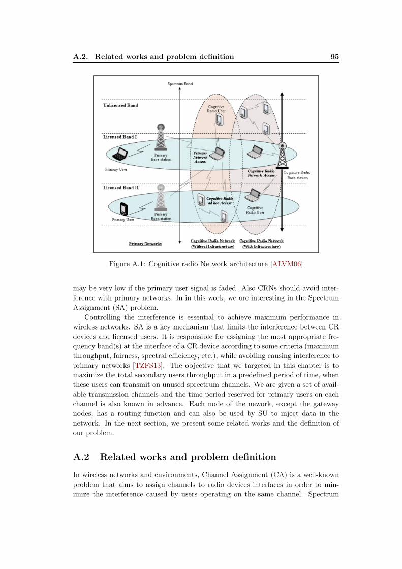
A.2. Related works and problem definition 95
Figure A.1: Cognitive radio Network architecture [ALVM06]
may be very low if the primary user signal is faded. Also CRNs should avoid inter-ference with primary networks. In in this work, we are interesting in the SpectrumAssignment (SA) problem.
Controlling the interference is essential to achieve maximum performance inwireless networks. SA is a key mechanism that limits the interference between CRdevices and licensed users. It is responsible for assigning the most appropriate fre-quency band(s) at the interface of a CR device according to some criteria (maximumthroughput, fairness, spectral efficiency, etc.), while avoiding causing interference toprimary networks [TZFS13]. The objective that we targeted in this chapter is tomaximize the total secondary users throughput in a predefined period of time, whenthese users can transmit on unused sprectrum channels. We are given a set of avail-able transmission channels and the time period reserved for primary users on eachchannel is also known in advance. Each node of the nework, except the gatewaynodes, has a routing function and can also be used by SU to inject data in thenetwork. In the next section, we present some related works and the definition ofour problem.
A.2 Related works and problem definition
In wireless networks and environments, Channel Assignment (CA) is a well-knownproblem that aims to assign channels to radio devices interfaces in order to min-imize the interference caused by users operating on the same channel. Spectrum
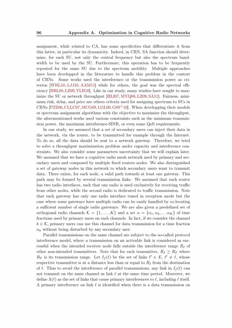
96 Appendix A. Optimization in Cognitive Radio Networks
assignment, while related to CA, has some specificities that differentiate it fromthis latter, in particular its dynamicity. Indeed, in CRN, SA function should deter-mine, for each SU, not only the central frequency but also the spectrum band-width to be used by the SU. Furthermore, this operation has to be frequentlyrepeated for the same SU due to the spectrum mobility. Multiple approacheshave been developped in the litterature to handle this problem in the contextof CRNs. Some works used the interference or the transmission power as cri-terion [WRL10, LJJ10, AAM11] while for others, the goal was the spectral effi-ciency [BBL08,LZ09,YLH10]. Like in our study, many studies have sought to max-imize the SU or network throughput [HLI07,MYQ08,LZ09, SA11]. Fairness, mini-mum risk, delay, and price are others criteria used for assigning spectrum to SUs inCRNs [PZZ06,CLLC07,MCG09,LGL09,GSS+10]. When developping their modelsor spectrum assignment algorithms with the objective to maximize the throughput,the aforementioned works used various constraints such as the minimum transmis-sion power, the maximum interference-SINR, or even some QoS requirements.
In our study, we assumed that a set of secondary users can inject their data inthe network, via the router, to be transmitted for example through the Internet.To do so, all the data should be sent to a network gateway. Therefore, we triedto solve a throughput maximization problem under capacity and interference con-straints. We also consider some parameters uncertainty that we will explain later.We assumed that we have a cognitive radio mesh network used by primary and sec-ondary users and composed by multiple fixed routers nodes. We also distinguisheda set of gateway nodes in this network to which secondary users want to transmitdata. There exists, for each node, a valid path towards at least one gateway. Thispath may be formed by several transmission links. We assumed that each routerhas two radio interfaces, such that one radio is used exclusively for receiving trafficfrom other nodes, while the second radio is dedicated to traffic transmission. Notethat each gateway has only one radio interface tuned in reception mode but thecase where some gateways have multiple radio can be easily handled by co-locatinga sufficient number of single radio gateways. We are also given a predefined set oforthogonal radio channels K = {1, . . . ,K} and a set α = {α1, α2, . . . αK} of timefractions used by primary users on each channels. In fact, if we consider the channelk ∈ K, primary users can use this channel for data transmission for a time fractionαk without being disturbed by any secondary user.
Parallel transmissions on the same channel are subject to the so-called protocolinterference model, where a transmission on an activable link is considered as suc-cessful when the intended receiver node falls outside the interference range RI ofother non-intended transmitters. Note that for each transmitter, RI ≥ RT whereRT is its transmission range. Let If (`) be the set of links `′ ∈ E, `′ 6= `, whoserespective transmitter is at a distance less than or equal to RI from the destinationof `. Thus to avoid the interference of parallel transmissions, any link in If (`) cannot transmit on the same channel as link ` at the same time period. Moreover, wedefine Λ(`) as the set of links that cause primary interferences to `, including ` itself.A primary interference on link ` is identified when there is a data transmission on
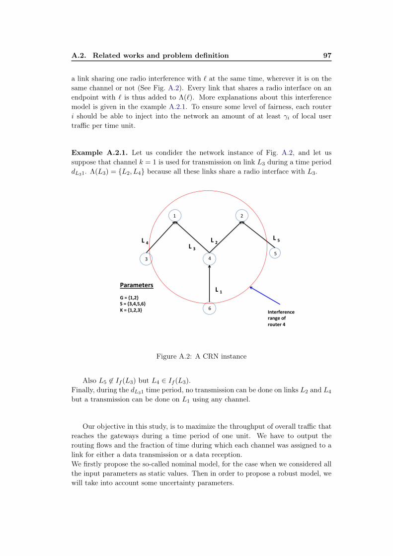
A.2. Related works and problem definition 97
a link sharing one radio interference with ` at the same time, wherever it is on thesame channel or not (See Fig. A.2). Every link that shares a radio interface on anendpoint with ` is thus added to Λ(`). More explanations about this interferencemodel is given in the example A.2.1. To ensure some level of fairness, each routeri should be able to inject into the network an amount of at least γi of local usertraffic per time unit.
Example A.2.1. Let us condider the network instance of Fig. A.2, and let ussuppose that channel k = 1 is used for transmission on link L3 during a time perioddL31. Λ(L3) = {L2, L4} because all these links share a radio interface with L3.
3
1
4
2
5
6
L 1
L 2 L 3
L 4 L 5
Parameters G = {1,2} S = {3,4,5,6} K = {1,2,3} Interference
range of router 4
Figure A.2: A CRN instance
Also L5 6∈ If (L3) but L4 ∈ If (L3).Finally, during the dL31 time period, no transmission can be done on links L2 and L4
but a transmission can be done on L1 using any channel.
Our objective in this study, is to maximize the throughput of overall traffic thatreaches the gateways during a time period of one unit. We have to output therouting flows and the fraction of time during which each channel was assigned to alink for either a data transmission or a data reception.We firstly propose the so-called nominal model, for the case when we considered allthe input parameters as static values. Then in order to propose a robust model, wewill take into account some uncertainty parameters.
98 Appendix A. Optimization in Cognitive Radio Networks
A.3 Nominal model
This network is represented as a directed graph D = (S ∪G,E) where S is the setof routers that injects in the network and relay the traffic of secondary users, and Gis the set of gateways nodes. E represents the sets of activable links in D, i.e., linkswhere the distance between the origin and the destination is less than RT . Becauseof the spectrum mobility in CRN, a channel is not assigned to a unique SU for thewhole transmission time like in traditional wireless networks. Instead we considerthat one SU can use channel c1 to transmit for time period d1 and then channel c2
for another time period d2 and so on. So in our model, what matters is the timeperiod during which a link has used a channel to transmit or to receive data. Inthe sequel, the transmitter and the receiver of a link ` are denoted by t(`) and r(`),respectively.
To model properly our problem, we need to define the following variables:
• f` represents for each link ` ∈ E, the traffic flow transmitted from router t(`)to router r(`) during a time unit.
• d`k denotes for each link ` ∈ E and each channel k in {1, . . . ,K}, the timefraction where link ` is activated on channel k.
The data rate that can be supported on a link ` per time unit is denoted asθ`. We assume that as long as a primary user is transmitting over a channel, allsecondary users must remain silent on that channel. Now, the problem could bestated as follows:
Model (1)
max∑`∈Er(`)∈G
f` (A.1)
s.t. ∑`∈E,r(`)=i
f` −∑
`∈E,t(`)=i
f` ≤ −γi, ∀ i ∈ S (A.2.1)
f` ≤ θ`K∑k=1
d`k ∀` ∈ E (A.2.2)
d`k +∑
`′∈If (`)
d`′k +K∑
k′=1,k′ 6=k
∑`′∈Λ(`)
d`′k′ ≤ 1− αk ∀ ` ∈ E, k = 1, . . . ,K (A.2.3)
f` ≥ 0 ∀ ` ∈ E (A.2.4)
d`k ≥ 0 ∀ ` ∈ E,∀ k = 1, . . . ,K (A.2.5)
Constraint (A.2.1) states that the difference between outgoing and ingoing flowson a router must be at least γi. Constraint (A.2.2) expresses that the flow routed
A.4. Robust model 99
on link ` should be at most equal to its capacity calculated as the product of θ` andthe sum of time period in which a channel is assigned to this link. θ` representshere the capacity of each link in terms of the number of packets per time unit.Constraint (A.2.3) provides a sufficient condition on each channel k so that a givenlink ` with transmission duration fraction d`,k could be scheduled with both primaryand secondary interfering links in non-overlapping time intervals. This constraintalso considers the time fraction αk reserved to primary users. For instance, thisconstraint expresses the impossibility of transmission by links in If (`) using channelk and by links in Λ(`) using any channel during the time period when a link ` istransmitting over channel k. Moreover, with these d`k, we are able to establish achannel assignment scheduling in the total transmission period without any conflict.
A.4 Robust model
In the sequel, we assume there exists m primary users. Each such user may possiblytransmits on any channel k = 1 . . .K, but with a known time fraction equal to λp(p = 1, . . . ,m). Hence, the vector α = (α1, α2, . . . , αK) denoting the time fractionoccupied by primary users becomes uncertain. This vector belongs to an uncertaintyset β defined with the binary parameters bpk which indicate if primary user p istransmitting on channel k. In particular, each element αk is upper bounded by 1and defined as:
αk =
m∑p=1
bpkλp (A.3)
where the parameters bpk are subject to the following constraint that states thata primary user occupies at most one channel at the time:
K∑k=1
bpk ≤ 1, p = 1 . . .m (A.4)
To handle the parameters uncertainty, a branch of Operational Research has pro-posed multiple methods using robust linear programming [Soy73,BTEGN09,BS04,Min11]. These works are different from stochastic programming methods which relyon probability distributions of uncertain problem parameters. Two classes of robustoptimization methods can be distinguished: those using column-wise uncertaintyand those using row-wise uncertainty. Our model falls inside the class of robust LPwith RHS uncertainty which is a particular type of column-wise uncertainty.
Our model can be viewed as a problem in which the process of decision-makingunder uncertainty can be decomposed in two successive steps (two-stage decisionmaking). For instance, in the first stage and without knowing any realization of theuncertainty, we can guarantee a certain throughput for the network. Then, afterthe realization of the uncertainty, the goal would be to find a channel assignment
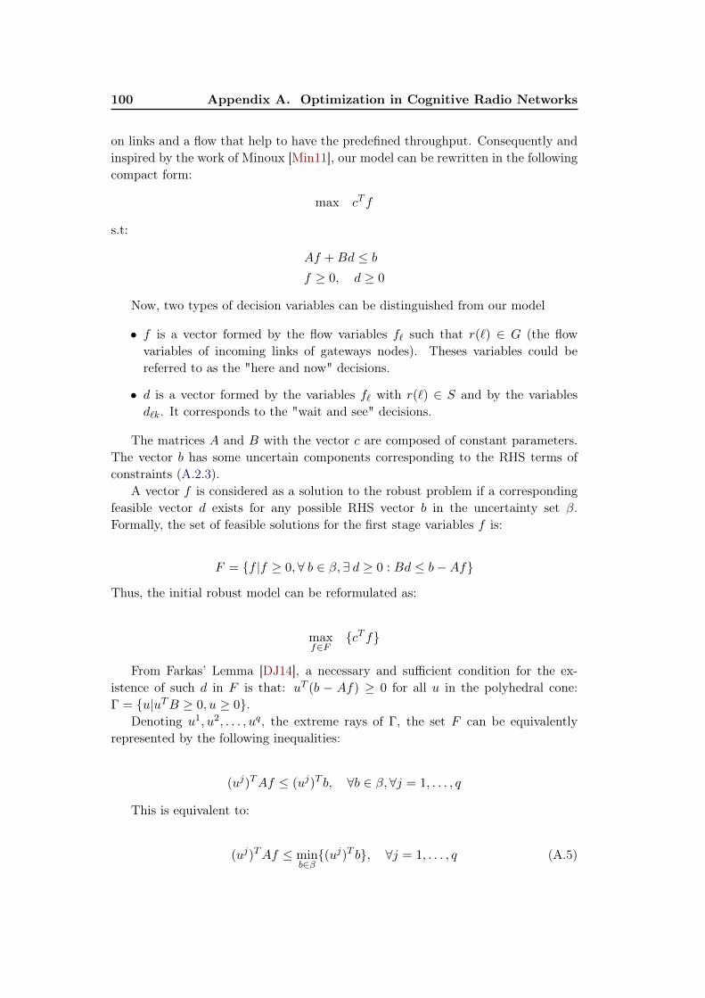
100 Appendix A. Optimization in Cognitive Radio Networks
on links and a flow that help to have the predefined throughput. Consequently andinspired by the work of Minoux [Min11], our model can be rewritten in the followingcompact form:
max cT f
s.t:
Af +Bd ≤ bf ≥ 0, d ≥ 0
Now, two types of decision variables can be distinguished from our model
• f is a vector formed by the flow variables f` such that r(`) ∈ G (the flowvariables of incoming links of gateways nodes). Theses variables could bereferred to as the "here and now" decisions.
• d is a vector formed by the variables f` with r(`) ∈ S and by the variablesd`k. It corresponds to the "wait and see" decisions.
The matrices A and B with the vector c are composed of constant parameters.The vector b has some uncertain components corresponding to the RHS terms ofconstraints (A.2.3).
A vector f is considered as a solution to the robust problem if a correspondingfeasible vector d exists for any possible RHS vector b in the uncertainty set β.Formally, the set of feasible solutions for the first stage variables f is:
F = {f |f ≥ 0, ∀ b ∈ β,∃ d ≥ 0 : Bd ≤ b−Af}
Thus, the initial robust model can be reformulated as:
maxf∈F
{cT f}
From Farkas’ Lemma [DJ14], a necessary and sufficient condition for the ex-istence of such d in F is that: uT (b − Af) ≥ 0 for all u in the polyhedral cone:Γ = {u|uTB ≥ 0, u ≥ 0}.
Denoting u1, u2, . . . , uq, the extreme rays of Γ, the set F can be equivalentlyrepresented by the following inequalities:
(uj)TAf ≤ (uj)T b, ∀b ∈ β,∀j = 1, . . . , q
This is equivalent to:
(uj)TAf ≤ minb∈β{(uj)T b}, ∀j = 1, . . . , q (A.5)
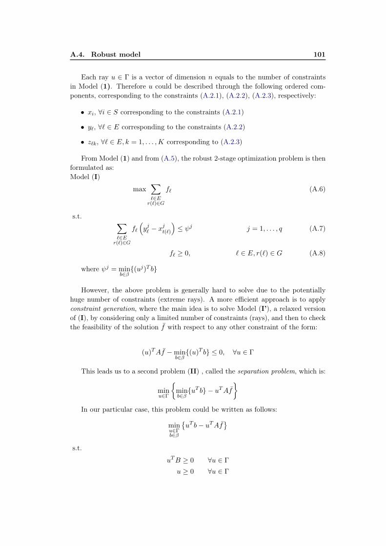
A.4. Robust model 101
Each ray u ∈ Γ is a vector of dimension n equals to the number of constraintsin Model (1). Therefore u could be described through the following ordered com-ponents, corresponding to the constraints (A.2.1), (A.2.2), (A.2.3), respectively:
• xi, ∀i ∈ S corresponding to the constraints (A.2.1)
• y`, ∀` ∈ E corresponding to the constraints (A.2.2)
• z`k, ∀` ∈ E, k = 1, . . . ,K corresponding to (A.2.3)
From Model (1) and from (A.5), the robust 2-stage optimization problem is thenformulated as:Model (I)
max∑`∈Er(`)∈G
f` (A.6)
s.t. ∑`∈Er(`)∈G
f`
(yj` − x
jt(`)
)≤ ψj j = 1, . . . , q (A.7)
f` ≥ 0, ` ∈ E, r(`) ∈ G (A.8)
where ψj = minb∈β{(uj)T b}
However, the above problem is generally hard to solve due to the potentiallyhuge number of constraints (extreme rays). A more efficient approach is to applyconstraint generation, where the main idea is to solve Model (I’), a relaxed versionof (I), by considering only a limited number of constraints (rays), and then to checkthe feasibility of the solution f with respect to any other constraint of the form:
(u)TAf −minb∈β{(u)T b} ≤ 0, ∀u ∈ Γ
This leads us to a second problem (II) , called the separation problem, which is:
minu∈Γ
{minb∈β{uT b} − uTAf
}In our particular case, this problem could be written as follows:
minu∈Γb∈β
{uT b− uTAf
}s.t.
uTB ≥ 0 ∀u ∈ Γ
u ≥ 0 ∀u ∈ Γ
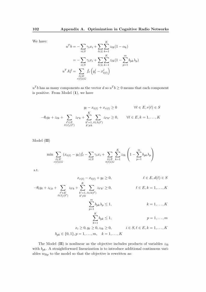
102 Appendix A. Optimization in Cognitive Radio Networks
We have:uT b = −
∑i∈S
γixi +∑`∈L
K∑k=1
z`k(1− αk)
= −∑i∈S
γixi +∑`∈L
K∑k=1
z`k(1−m∑p=1
bpkλp)
uTAf =∑`∈Er(`)∈G
f`
(yj` − x
jt(`)
)
uT b has as many components as the vector d so uT b ≥ 0 means that each componentis positive. From Model (1), we have
yl − xt(`) + xr(`) ≥ 0 ∀` ∈ E, r(`) ∈ S
−θ`y` + z`k +∑`′∈E
`∈If (`′)
z`′k +
K∑k′=1,k′ 6=k
∑`∈Λ(`′)
z`′k′ ≥ 0, ∀` ∈ E, k = 1, . . . ,K
Model (II)
min∑`∈Er(`)∈G
(xt(`) − y`)f` −∑i∈S
γixi +∑`∈Et(`)∈G
K∑k=1
z`k
1−m∑p=1
bpkλp
s.t.
xr(`) − xt(`) + y` ≥ 0, ` ∈ E, d(`) ∈ S
−θ`y` + z`,k +∑`′∈E
`∈If (`′)
z`′k +K∑
k′=1,k′ 6=k
∑`∈Λ(`′)
z`′k′ ≥ 0, ` ∈ E, k = 1, . . . ,K
m∑p=1
bpkλp ≤ 1, k = 1, . . . ,K
K∑k=1
bpk ≤ 1, p = 1, . . . ,m
xi ≥ 0, y` ≥ 0, z`k ≥ 0, i ∈ S, ` ∈ E, k = 1, . . . ,K
bpk ∈ {0, 1}, p = 1, . . . ,m, k = 1, . . . ,K
The Model (II) is nonlinear as the objective includes products of variables z`kwith bpk. A straightforward linearization is to introduce additional continuous vari-ables wlkp to the model so that the objective is rewritten as:
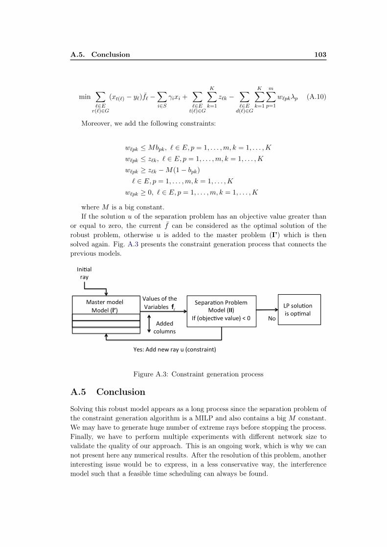
A.5. Conclusion 103
min∑`∈Er(`)∈G
(xt(`) − y`)f` −∑i∈S
γixi +∑`∈Et(`)∈G
K∑k=1
z`k −∑`∈Ed(`)∈G
K∑k=1
m∑p=1
w`pkλp (A.10)
Moreover, we add the following constraints:
w`pk ≤Mbpk, ` ∈ E, p = 1, . . . ,m, k = 1, . . . ,K
w`pk ≤ z`k, ` ∈ E, p = 1, . . . ,m, k = 1, . . . ,K
w`pk ≥ z`k −M(1− bpk)` ∈ E, p = 1, . . . ,m, k = 1, . . . ,K
w`pk ≥ 0, ` ∈ E, p = 1, . . . ,m, k = 1, . . . ,K
where M is a big constant.If the solution u of the separation problem has an objective value greater than
or equal to zero, the current f can be considered as the optimal solution of therobust problem, otherwise u is added to the master problem (I’) which is thensolved again. Fig. A.3 presents the constraint generation process that connects theprevious models.
Figure A.3: Constraint generation process
A.5 Conclusion
Solving this robust model appears as a long process since the separation problem ofthe constraint generation algorithm is a MILP and also contains a big M constant.We may have to generate huge number of extreme rays before stopping the process.Finally, we have to perform multiple experiments with different network size tovalidate the quality of our approach. This is an ongoing work, which is why we cannot present here any numerical results. After the resolution of this problem, anotherinteresting issue would be to express, in a less conservative way, the interferencemodel such that a feasible time scheduling can always be found.

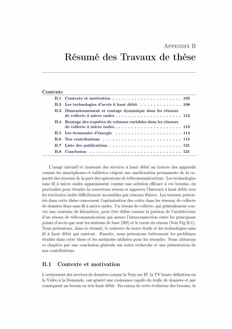
Appendix B
Résumé des Travaux de thèse
ContentsB.1 Contexte et motivation . . . . . . . . . . . . . . . . . . . . . . 105
B.2 Les technologies d’accès à haut débit . . . . . . . . . . . . . 108
B.3 Dimensionnement et routage dynamique dans les réseauxde collecte à micro ondes . . . . . . . . . . . . . . . . . . . . . 112
B.4 Routage des requêtes de volumes variables dans les réseauxde collecte à micro ondes . . . . . . . . . . . . . . . . . . . . . 113
B.5 Les économies d’énergie . . . . . . . . . . . . . . . . . . . . . 114
B.6 Nos contributions . . . . . . . . . . . . . . . . . . . . . . . . . 115
B.7 Liste des publications . . . . . . . . . . . . . . . . . . . . . . . 121
B.8 Conclusion . . . . . . . . . . . . . . . . . . . . . . . . . . . . . 121
L’usage intensif et croissant des services à haut débit au travers des appareilscomme les smartphones et tablettes exigent une amélioration permanente de la ca-pacité des réseaux de la part des opérateurs de télécommunications. Les technologiessans fil à micro ondes apparaisssent comme une solution efficace à ces besoins, enparticulier pour étendre la couverture réseau et apporter l’Internet à haut débit versles territoires isolés difficilement accessibles par réseaux filaires. Les travaux présen-tés dans cette thèse concernent l’optimisation des coûts dans les réseaux de collectede données fixes sans fil à micro ondes. Un réseau de collecte, qui généralement cou-vre une centaine de kilomètres, peut être défini comme la portion de l’architectured’un réseau de télécommunication qui assure l’interconnection entre les principauxpoints d’accès que sont les stations de base (BS) et le coeur du réseau (Voir Fig B.1).Nous présentons, dans ce résumé, le contexte de notre étude et les technologies sansfil à haut débit qui existent. Ensuite, nous présentons brièvement les problèmesétudiés dans cette thèse et les méthodes utilisées pour les résoudre. Nous clôturonsce chapitre par une conclusion générale sur notre recherche et une présentation denos contributions.
B.1 Contexte et motivation
L’avènement des services de données comme la Voix sur IP, la TV haute définition oula Vidéo à la Demande, ont généré une croissance rapide du trafic de données et parconséquent un besoin en très haut débit. En raison de cette évolution des besoins, la
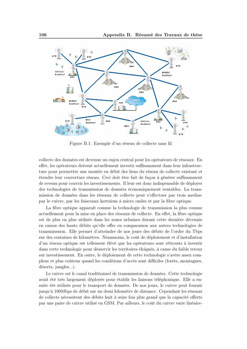
106 Appendix B. Résumé des Travaux de thèse
Figure B.1: Exemple d’un réseau de collecte sans fil
collecte des données est devenue un enjeu central pour les opérateurs de réseaux. Eneffet, les opérateurs doivent actuellement investir suffisamment dans leur infrastruc-ture pour permettre une montée en débit des liens du réseau de collecte existant etétendre leur couverture réseau. Ceci doit être fait de façon à générer suffisammentde revenu pour couvrir les investissements. Il leur est donc indispensable de déployerdes technologies de transmission de données économiquement rentables. La trans-mission de données dans les réseaux de collecte peut s’effectuer par trois medias:par le cuivre, par les faisceaux hertziens à micro ondes et par la fibre optique.
La fibre optique apparaît comme la technologie de transmission la plus connueactuellement pour la mise en place des réseaux de collecte. En effet, la fibre optiqueest de plus en plus utilisée dans les zones urbaines durant cette dernière décennieen raison des hauts débits qu’elle offre en comparaison aux autres technologies detransmisssion. Elle permet d’atteindre de nos jours des débits de l’ordre du Tbpssur des centaines de kilomètres. Néanmoins, le coût de déploiement et d’installationd’un réseau optique est tellement élévé que les opérateurs sont réticents à investirdans cette technologie pour désservir les territoires éloignés, à cause du faible retoursur investissement. En outre, le déploiement de cette technologie s’avère assez com-plexe et plus coûteux quand les conditions d’accès sont difficiles (forêts, montagnes,déserts, jungles...).
Le cuivre est le canal traditionnel de transmission de données. Cette technologieavait été très largement déployée pour établir les liaisons téléphonique. Elle a en-suite été utilisée pour le transport de données. De nos jours, le cuivre peut fournirjusqu’à 100Mbps de débit sur un demi kilomètre de distance. Cependant les réseauxde collecte nécessitent des débits huit à seize fois plus grand que la capacité offertepar une paire de cuivre utilisé en GSM. Par ailleurs, le coût du cuivre varie linéaire-
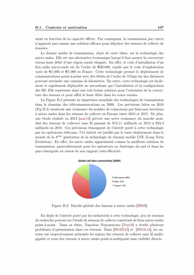
B.1. Contexte et motivation 107
ment en fonction de la capacité offerte. Par conséquent, la transmission par cuivren’apparait pas comme une solution efficace pour dépolyer des réseaux de collecte dedonnées.
Le dernier média de transmission, objet de cette thèse, est la technologie desmicro ondes. Elle est une alternative économique lorsqu’il faut assurer la couvertureréseau haut débit d’une région rurale éloignée. En effet, le coût d’installation d’unlien radio micro-onde est de l’ordre de e20.000, tandis que le coût d’exploitationvarie de e1.000 et e5.000 en France. Cette technologie permet le déploiement decommunications point-à-point avec des débits de l’ordre de 1Gbps sur des distancespouvant atteindre une centaine de kilomètres. En outre, cette technologie est facile-ment et rapidement déployable ne nécessitant que l’installation et la configurationdes BS. Elle représente ainsi une très bonne solution pour l’extension de la couver-ture des réseaux et pour offrir le haut débit dans les zones rurales.
La Figure B.2 présente la répartition mondiale des technologies de transmissiondans le domaine des télécommunications en 2009. Les prévisions faites en 2010(Fig B.3) montrent une croissance du nombre de connexions par faisceaux hertziensà micro ondes dans les réseaux de collecte en Europe entre 2010 et 2015. De plus,une étude réalisée en 2013 [mar13] prévoit une nette croissance du marché mon-dial des réseaux de collectes sans fil passant de $13.11 milliards en 2013 à $23.3milliards en 2018. Ces prévisions témoignent de l’intérêt porté à cette technologiepar les opérateurs télécoms. Cet intérêt est justifié par le vaste déploiement dans lemonde de la 4ime génération de la technologie de réseaux mobile LTE (Long TermEvolution). En effet, les micro ondes apparaissent comme la meilleure solution detransmission, particulièrement pour les opérateurs en Amérique du sud et dans lespays émergents en raison de son rapport coût-efficacité.
Figure B.2: Marché globale des liaisons à micro ondes [HR09]
En dépit de l’intérêt porté par les industriels à cette technologie, peu de travauxde recherche portent sur l’étude de réseaux de collecte constitués de liens micro-ondespoint-à-point. Dans sa thèse, Napoleao Nepomuceno [Nep10] a étudié plusieursproblèmes d’optimisation dans ces réseaux. Dans [HGZD12] et [HEOL13], les au-teurs ont respectivement présentés les enjeux des réseaux de collecte sans fil multi-gigabit et ceux des réseaux à micro ondes point-à-multipoint sans visibilté directe.
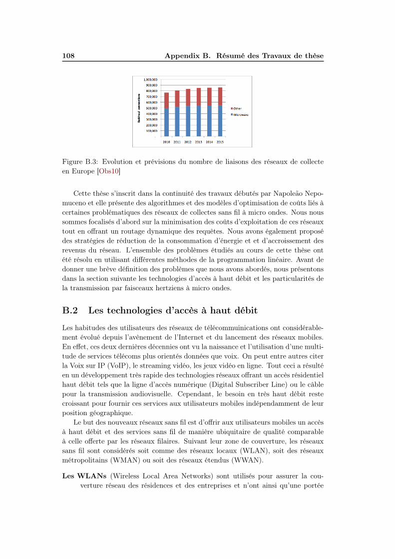
108 Appendix B. Résumé des Travaux de thèse
Figure B.3: Evolution et prévisions du nombre de liaisons des réseaux de collecteen Europe [Obs10]
Cette thèse s’inscrit dans la continuité des travaux débutés par Napoleão Nepo-muceno et elle présente des algorithmes et des modèles d’optimisation de coûts liés àcertaines problématiques des réseaux de collectes sans fil à micro ondes. Nous noussommes focalisés d’abord sur la minimisation des coûts d’exploitation de ces réseauxtout en offrant un routage dynamique des requêtes. Nous avons également proposédes stratégies de réduction de la consommation d’énergie et et d’accroissement desrevenus du réseau. L’ensemble des problèmes étudiés au cours de cette thèse ontété résolu en utilisant différentes méthodes de la programmation linéaire. Avant dedonner une brève définition des problèmes que nous avons abordés, nous présentonsdans la section suivante les technologies d’accès à haut débit et les particularités dela transmission par faisceaux hertziens à micro ondes.
B.2 Les technologies d’accès à haut débit
Les habitudes des utilisateurs des réseaux de télécommuinications ont considérable-ment évolué depuis l’avènement de l’Internet et du lancement des réseaux mobiles.En effet, ces deux dernières décennies ont vu la naissance et l’utilisation d’une multi-tude de services télécoms plus orientés données que voix. On peut entre autres citerla Voix sur IP (VoIP), le streaming vidéo, les jeux vidéo en ligne. Tout ceci a résultéen un développement très rapide des technologies réseaux offrant un accès résidentielhaut débit tels que la ligne d’accès numérique (Digital Subscriber Line) ou le câblepour la transmission audiovisuelle. Cependant, le besoin en très haut débit restecroissant pour fournir ces services aux utilisateurs mobiles indépendamment de leurposition géographique.
Le but des nouveaux réseaux sans fil est d’offrir aux utilisateurs mobiles un accèsà haut débit et des services sans fil de manière ubiquitaire de qualité comparableà celle offerte par les réseaux filaires. Suivant leur zone de couverture, les réseauxsans fil sont considérés soit comme des réseaux locaux (WLAN), soit des réseauxmétropolitains (WMAN) ou soit des réseaux étendus (WWAN).
Les WLANs (Wireless Local Area Networks) sont utilisés pour assurer la cou-verture réseau des résidences et des entreprises et n’ont ainsi qu’une portée
B.2. Les technologies d’accès à haut débit 109
d’environ une centaine de mètres. Ils offrent des débits pouvant atteindre100Mbps avec le 802.11n [VN10] et sont utilisés au travers de points d’accèsauxquels peuvent se connecter les stations de travail. La technologie WLANla plus répandue est le IEEE 802.11 plus connu sous le nom de WiFi. Maisdans ce type de réseaux nous dinstinguons également la technologie HiperLAN(High Performance Radio LAN) [Joh99,DAB+02]. Notons qu’il est égalementpossible de configurer les WLANs en mode ad hoc de sorte que toutes les sta-tions puissent communiquer directement entre elles sans passer par un pointd’accès.
Les WMANs (Wireless Metropolitan Area Networks) sont des réseaux permettantaux utilisateurs d’établir des connexions sans fil entre plusieurs emplacementsau sein d’une région urbaine. Par conséquent, ces réseaux couvrent des zonesde la taille d’une ville. Ils permettent d’interconnecter plusieurs WLANs.Plusieurs technologies ont été développées dans le contexte des WMANs, lesplus répandues étant les réseaux de la famille IEEE801.16-WiMax, les réseauxHiperMANs et le Hiper Acces. Ils fournissent une connectivité à haut débitaux utilisateurs fixes, en visibilité directe ou non mais aussi aux utilisateursmobiles. Ils fonctionnent sur le principe de couverture cellulaire assurée parles stations de bases auxquelles se connectent les stations d’abonnés pouvantetre des immeubles ou des véhicules, soit en mode point à point ou point àmultipoint. Les WMANs supportent également les topologies maillées doncsans insfrastructures. Le Wimax fournit un débit aggrégé de 135Mbps suivantla modulation utilisée en visibilité directe alors qu’un débit allant jusqu’à75Mbps peut être atteint pour des communications en absence de visibilitédirecte. Les réseaux HiperMANs peuvent supporter des débits de 25Mbpspour chaque secteur du point d’accès. Le lecteur est invité à se reporter à[KT07] pour plus de détails sur ces technologies.
Les WWANs (Wireless Wide Area Networks) sont communément utilisés pourconnecter différents WMANs situés dans des régions assez éloignées. Ils sontprincipalement constitués de systèmes satellitaires utilisés essentiellement entransmission descendante. Le IEEE802.20 connu sous le nom de Réseauxmobile sans fil à haut débit (MBWA) est une autre technologie WWAN. Sonobjectif principal est de fournir un accès haut débit aux appareils hautementmobiles et se déplaçant à des vitesses de l’ordre de 250km/h comme les voitureset trains [BXG07].
Pour résumer, Les utilisateurs transmettent grâce aux WLANs leurs données quisont aggrégées et transmis à travers les réseaux WMANs vers l’Internet. Ensuiteles WWANs assurent l’interconnection entre plusieurs WMANs de diverses zones dumonde. En dehors des technologies mentionnées précemment, on distingue aussi lestechnologies mobiles tels que les systèmes 3G (UMTS, HSPA, CDMA2000, EV-DO)et 4G (LTE, LTE-Avancé) qui sont également considérés comme des réseaux sansfil à haut débit. En effet, ils fournissent des débits pouvant atteindre 14,4 Mbps
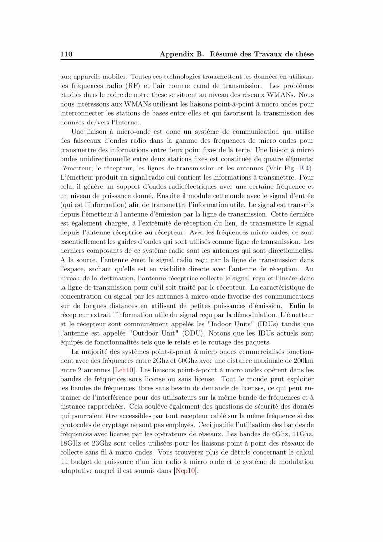
110 Appendix B. Résumé des Travaux de thèse
aux appareils mobiles. Toutes ces technologies transmettent les données en utilisantles fréquences radio (RF) et l’air comme canal de transmission. Les problèmesétudiés dans le cadre de notre thèse se situent au niveau des réseaux WMANs. Nousnous intéressons aux WMANs utilisant les liaisons point-à-point à micro ondes pourinterconnecter les stations de bases entre elles et qui favorisent la transmission desdonnées de/vers l’Internet.
Une liaison à micro-onde est donc un système de communication qui utilisedes faisceaux d’ondes radio dans la gamme des fréquences de micro ondes pourtransmettre des informations entre deux point fixes de la terre. Une liaison à microondes unidirectionnelle entre deux stations fixes est constituée de quatre éléments:l’émetteur, le récepteur, les lignes de transmission et les antennes (Voir Fig. B.4).L’émetteur produit un signal radio qui contient les informations à transmettre. Pourcela, il génère un support d’ondes radioélectriques avec une certaine fréquence etun niveau de puissance donné. Ensuite il module cette onde avec le signal d’entrée(qui est l’information) afin de transmettre l’information utile. Le signal est transmisdepuis l’émetteur à l’antenne d’émission par la ligne de transmission. Cette dernièreest également chargée, à l’extrémité de réception du lien, de transmettre le signaldepuis l’antenne réceptrice au récepteur. Avec les fréquences micro ondes, ce sontessentiellement les guides d’ondes qui sont utilisés comme ligne de transmission. Lesderniers composants de ce système radio sont les antennes qui sont directionnelles.A la source, l’antenne émet le signal radio reçu par la ligne de transmission dansl’espace, sachant qu’elle est en visibilité directe avec l’antenne de réception. Auniveau de la destination, l’antenne réceptrice collecte le signal reçu et l’insère dansla ligne de transmission pour qu’il soit traité par le récepteur. La caractéristique deconcentration du signal par les antennes à micro onde favorise des communicationssur de longues distances en utilisant de petites puissances d’émission. Enfin lerécepteur extrait l’information utile du signal reçu par la démodulation. L’émetteuret le récepteur sont communément appelés les "Indoor Units" (IDUs) tandis quel’antenne est appelée "Outdoor Unit" (ODU). Notons que les IDUs actuels sontéquipés de fonctionnalités tels que le relais et le routage des paquets.
La majorité des systèmes point-à-point à micro ondes commercialisés fonction-nent avec des fréquences entre 2Ghz et 60Ghz avec une distance maximale de 200kmentre 2 antennes [Leh10]. Les liaisons point-à-point à micro ondes opèrent dans lesbandes de fréquences sous license ou sans license. Tout le monde peut exploiterles bandes de fréquences libres sans besoin de demande de licenses, ce qui peut en-trainer de l’interférence pour des utilisateurs sur la même bande de fréquences et àdistance rapprochées. Cela soulève également des questions de sécurité des donnésqui pourraient être accessibles par tout recepteur cablé sur la même fréquence si desprotocoles de cryptage ne sont pas employés. Ceci justifie l’utilisation des bandes defréquences avec license par les opérateurs de réseaux. Les bandes de 6Ghz, 11Ghz,18GHz et 23Ghz sont celles utilisées pour les liaisons point-à-point des réseaux decollecte sans fil à micro ondes. Vous trouverez plus de détails concernant le calculdu budget de puissance d’un lien radio à micro onde et le système de modulationadaptative auquel il est soumis dans [Nep10].
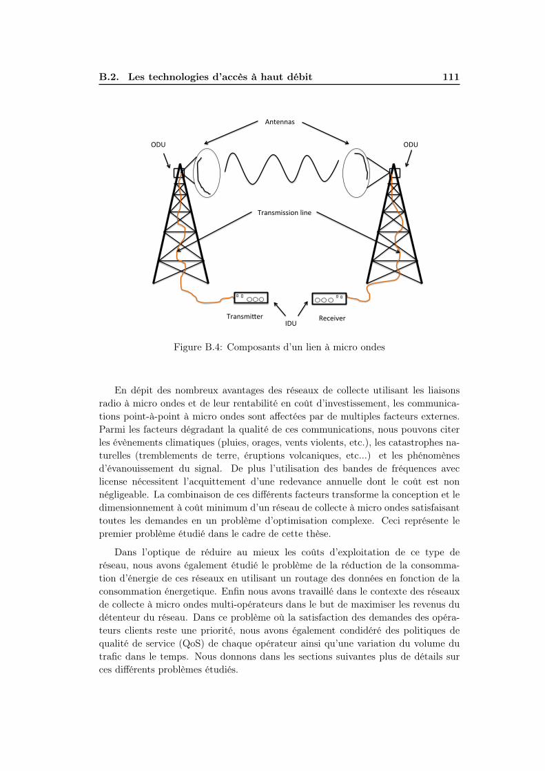
B.2. Les technologies d’accès à haut débit 111
Transmi(er Receiver
Antennas
Transmission line
ODU ODU
IDU
Figure B.4: Composants d’un lien à micro ondes
En dépit des nombreux avantages des réseaux de collecte utilisant les liaisonsradio à micro ondes et de leur rentabilité en coût d’investissement, les communica-tions point-à-point à micro ondes sont affectées par de multiples facteurs externes.Parmi les facteurs dégradant la qualité de ces communications, nous pouvons citerles évènements climatiques (pluies, orages, vents violents, etc.), les catastrophes na-turelles (tremblements de terre, éruptions volcaniques, etc...) et les phénomènesd’évanouissement du signal. De plus l’utilisation des bandes de fréquences aveclicense nécessitent l’acquittement d’une redevance annuelle dont le coût est nonnégligeable. La combinaison de ces différents facteurs transforme la conception et ledimensionnement à coût minimum d’un réseau de collecte à micro ondes satisfaisanttoutes les demandes en un problème d’optimisation complexe. Ceci représente lepremier problème étudié dans le cadre de cette thèse.
Dans l’optique de réduire au mieux les coûts d’exploitation de ce type deréseau, nous avons également étudié le problème de la réduction de la consomma-tion d’énergie de ces réseaux en utilisant un routage des données en fonction de laconsommation énergetique. Enfin nous avons travaillé dans le contexte des réseauxde collecte à micro ondes multi-opérateurs dans le but de maximiser les revenus dudétenteur du réseau. Dans ce problème où la satisfaction des demandes des opéra-teurs clients reste une priorité, nous avons également condidéré des politiques dequalité de service (QoS) de chaque opérateur ainsi qu’une variation du volume dutrafic dans le temps. Nous donnons dans les sections suivantes plus de détails surces différents problèmes étudiés.
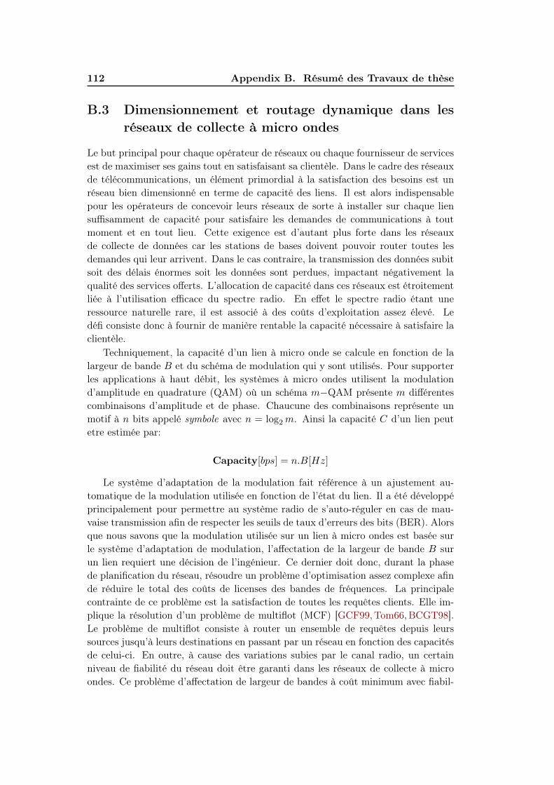
112 Appendix B. Résumé des Travaux de thèse
B.3 Dimensionnement et routage dynamique dans lesréseaux de collecte à micro ondes
Le but principal pour chaque opérateur de réseaux ou chaque fournisseur de servicesest de maximiser ses gains tout en satisfaisant sa clientèle. Dans le cadre des réseauxde télécommunications, un élément primordial à la satisfaction des besoins est unréseau bien dimensionné en terme de capacité des liens. Il est alors indispensablepour les opérateurs de concevoir leurs réseaux de sorte à installer sur chaque liensuffisamment de capacité pour satisfaire les demandes de communications à toutmoment et en tout lieu. Cette exigence est d’autant plus forte dans les réseauxde collecte de données car les stations de bases doivent pouvoir router toutes lesdemandes qui leur arrivent. Dans le cas contraire, la transmission des données subitsoit des délais énormes soit les données sont perdues, impactant négativement laqualité des services offerts. L’allocation de capacité dans ces réseaux est étroitementliée à l’utilisation efficace du spectre radio. En effet le spectre radio étant uneressource naturelle rare, il est associé à des coûts d’exploitation assez élevé. Ledéfi consiste donc à fournir de manière rentable la capacité nécessaire à satisfaire laclientèle.
Techniquement, la capacité d’un lien à micro onde se calcule en fonction de lalargeur de bande B et du schéma de modulation qui y sont utilisés. Pour supporterles applications à haut débit, les systèmes à micro ondes utilisent la modulationd’amplitude en quadrature (QAM) où un schéma m−QAM présente m différentescombinaisons d’amplitude et de phase. Chaucune des combinaisons représente unmotif à n bits appelé symbole avec n = log2m. Ainsi la capacité C d’un lien peutetre estimée par:
Capacity[bps] = n.B[Hz]
Le système d’adaptation de la modulation fait référence à un ajustement au-tomatique de la modulation utilisée en fonction de l’état du lien. Il a été développéprincipalement pour permettre au système radio de s’auto-réguler en cas de mau-vaise transmission afin de respecter les seuils de taux d’erreurs des bits (BER). Alorsque nous savons que la modulation utilisée sur un lien à micro ondes est basée surle système d’adaptation de modulation, l’affectation de la largeur de bande B surun lien requiert une décision de l’ingénieur. Ce dernier doit donc, durant la phasede planification du réseau, résoudre un problème d’optimisation assez complexe afinde réduire le total des coûts de licenses des bandes de fréquences. La principalecontrainte de ce problème est la satisfaction de toutes les requêtes clients. Elle im-plique la résolution d’un problème de multiflot (MCF) [GCF99,Tom66,BCGT98].Le problème de multiflot consiste à router un ensemble de requêtes depuis leurssources jusqu’à leurs destinations en passant par un réseau en fonction des capacitésde celui-ci. En outre, à cause des variations subies par le canal radio, un certainniveau de fiabilité du réseau doit être garanti dans les réseaux de collecte à microondes. Ce problème d’affectation de largeur de bandes à coût minimum avec fiabil-
B.4. Routage des requêtes de volumes variables dans les réseaux decollecte à micro ondes 113
ité a été étudié par Nepomuceno durant sa thèse [Nep10] en utilisant une approcheprobabilistique de chance-constrained programming.
Contrairement aux travaux de Nepomuceno, nous avons dans cette thèse résoluce problème en considérant un routage dynamique des demandes. Ainsi suivantles atténuations de signal sur les liens et les adaptations de modulation requises, lesrequêtes pourront etre re-acheminées suivant les nouvelles capacités des liens, modifi-ant ainsi les flots. Cette approche apporte beaucoup plus de souplesse dans le réseaucontrairement aux travaux précédents qui ont considéré un routage totalement sta-tique. Un unique schéma d’acheminement des données était utilisé indépendemmentde l’état du canal. Nous avons également modelisé ce problème de sorte à appliquersa solution à des réseaux de larges tailles, ce qui était difficilement possible. L’étudeet la résolution de ce problème ont été fait en collaboration avec Brigitte Jaumard(Université de Concordia, Montréal, Canada), Mejdi Kaddour (Université d’Oran,Algérie), Napoleão Nepomuceno (Univeristé de Fortaleza, Brésil) et David Coudert(Université de Nice Sophia Antipolis). Nous avons modélisé ce problème sous formed’un programme linéaire en nombre entiers mixtes (MILP). Il fut résolu en utilisantune méthode de génération de colonnes et une heuristique de recherche locale.
B.4 Routage des requêtes de volumes variables dans lesréseaux de collecte à micro ondes
Comme mentionné précédemment, les réseaux sans fil à micro onde représententune solution attractive pour les opérateurs afin de déployer leurs réseaux de col-lecte dans les zones rurales. Cependant, il peut s’avérer non rentable pour unopérateur de déployer sa propre infrastructure de réseaux de collecte à micro on-des, en particulier dans les zones à faible densité d’habitation à cause du faibleretour sur investissement. Une solution pour contourner cet obstacle est le conceptde partage d’infrastructure entre opérateurs proné par les autorités de régulationdepuis plusieurs années. Contrairement au partage de sites ou d’équipements queconseillent ces autorités, nous avons étudié le problème de partage de capacité duréseau entre plusieurs opérateurs. Dans le contexte d’un réseau de collecte déployépar un opérateur (le détenteur de l’infrastructure réseau) que nous nommons le PNO(Physical Network Operator), la capacité des liens de ce réseaux est louée à d’autresopérateurs virtuels VNOs(Virtual Network Operators) qui souhaitent acheminer lesrequêtes de leurs clients. L’objectif que nous avons visé est de maximiser le revenutotal du PNO sous les contraintes de satisfaction des demandes des VNOs tout enrespectant leurs différentes politiques de qualité de services. Nous avons en premierlieu formulé le problème en considérant des volumes de trafic fixes et de ce modèlenous avons déduit le modèle robuste dans lequel le volume de plusieurs requêtespeut varier. Ce problème étudié en collaboration avec David Coudert et ChristelleCaillouet (Université de Nice Sophia-Antipolis) a été résolu avec une formulation enprogramme linéaire en nombre entiers (ILP).
114 Appendix B. Résumé des Travaux de thèse
B.5 Les économies d’énergie
Dans la recherche de stratégies d’optimisation des coûts pour les réseaux de collectesans fil à micro ondes, la consommation d’énergie a été identifiée comme prenantune part non négligeable dans les coûts d’exploitation de ces réseaux. En 2011,Tombaz et al, dans leurs travaux [TMW+11] ont reporté que les communicationsmobiles occupent 0.05% de la consommation mondiale d’énergie et que 80% decette énergie provient des réseaux d’accès et plus précisément des stations de bases.Avec le grand nombre de stations de base à installer pour satisfaire la demandetoujours croissante en trafic, la consommation d’énergie des réseaux mobiles devraitdoubler d’ici 2020. Par conséquent la consommation d’énergie est amenée à devenirune problématique importante à régler pour les opérateurs télécoms afin de réduireleurs coûts d’exploitation. La recommandation R88 [All08, requirement R88] duforum des opérateurs mobiles appelé NGMN (Next Generation Mobile Networks)stipule que plusieurs modes de consommation d’énergie devraient être définies afinque les équipements des réseaux de collecte puissent automatiquement basculer verscelui qui permet de minimiser leur taux de consommation d’énergie. Les opérateursdoivent donc trouver les méchanismes pour adapter la consommation d’énergie desstations de base en fonction du volume de trafic en transit dans ces stations.
Ce problème de consommation d’énergie se pose également dans le "cœur" deréseau Internet. Basée sur des études récentes, la consommation d’énergie des in-frastructures d’Internet est estimée entre 1.1% et 1.9% des 16 TW que consommele monde [BAH+09,RM11,BHT11,HBF+11]. Dans [TBA+08], les auteurs ont re-marqué que la majeure partie de la consommation d’énergie de l’Internet provientdes réseaux d’accès et des routeurs. Ils ont prévu une augmentation rapide de cetteconsommation de 4% au vue de l’augmentation des débits d’accès transformant ainsiles routeurs IPs en goulots d’étranglement énergétique de l’Internet.
Une proposition pour limiter cette croissance de la consommation d’énergie estd’utiliser une technique de routage des données en fonction de la consommationd’énergie dans le réseau nommée EAR (Energy Aware Routing) [CSB+08,CMN09,BCRR12]. A cause de l’inexistence actuelle d’équipements permettant d’éteindre lesliens des réseaux de collecte, nous avons étudié ensemble avec Truong Khoa Phan(Université de Nice sophia Antipolis) l’optimisation de la consommation d’énergieappliquée aux réseaux backbones. Notre objectif était de minimiser la consommationd’énergie dans le réseau tout en étant en mesure de router l’ensemble des requêtes.Nous avons proposé plusieurs formulations du modèle en combinant l’utilisation del’EAR et d’une autre méthode, nommée RE (Redundancy Elimation) [AGA+08,ZCM11, ZA14] avec des valeurs de demandes fixes ou variables. Le problème futmodélisé dans sa forme robuste par des programmes linéaires en nombres entiersmixtes (MILP) et nous avons proposé différents algorithmes et heuristiques pour sarésolution. Ces travaux ont été effectué en espérant une application de cette méthodeaux réseaux de collecte sans fil une fois les équipements physiques disponibles.
L’ensemble des différents problèmes étudiés dans le cadre de cette thèse ontété modélisés en utilisant la programmation linéaire résultant ainsi en des modèles
B.6. Nos contributions 115
soit ILP ou MILP. Ensuite nous avons appliqué la méthode de la Γ−robustesseaux modèles contenant des variables dont les valeurs sont incertaines. Les solu-tions optimales obtenues grace aux modèles robustes restent réalisables et optimalesquelque soient les valeurs que prennent les variables incertaines. Enfin pour chaquemodèle proposé, un ensemble de tests numériques ont été effectués avec plusieursinstances de simulation de la librairy SNDlib [OWPT10] afin de déterminer lesforces et faiblesses des méthodes de résolution. Les différents algorithmes ont étéimplémentés soit en utilisant le langage de prommation Python, soit Java ou soitOPL(Optimization Programming Language). Ce dernier a la particularité d’êtreun langage de modélisation mathématique de haut niveau permettant une implé-mentation rapide d’algorithmes complexes tels que la génération de colonnes oude contraintes. Plus encore, ce langage est spécifiquement adapté à la rechercheopérationnelle (Programmation linéaire et programmation par contrainte) et offreune interface pour communiquer avec le solveurs CPLEX [II14] de IBM ILOG. Lesrésultats des simulations sont ensuite analysés suivant les différents paramètres enentrée au problème. Dans le cas où le modèle s’avère difficile à résoudre pour delarges instances, nous proposons, des heuristiques dont l’objectif est de trouver dessolutions réalisables proche de l’optimal dans des délais plus courts.
Dans la section suivante, nous présentons brièvement le développement de nostravaux de même que les résultats obtenus.
B.6 Nos contributions
Dans le Chapitre 2 de ce manuscrit, nous définissons en détail les concepts de laprogrammation linéaire. Nous avons également présenté la notion de la dualité etdeux théorèmes de la dualité qui nous ont été utiles durant nos travaux. Il s’agitde la dualité faible et de la dualité forte. Nous introduisons ensuite l’algorithmede génération de colonnes. Cet algorithme nous a été utile pour proposer une so-lution qui passe à l’échelle pour le problème de dimensionnement de réseau. Cetteméthode est essentiellement utilisée dans le cas de modèles linéaires contenant untrès grand nombre de variables. A l’optimum, la plupart des variables étant nulles,seul un petit sous-ensemble de variables doit être pris en compte pour résoudre leproblème. L’algorithme permet alors d’identifier uniquement les variables qui sontsusceptibles d’améliorer la solution courante. Nous présentons également en détaille sous-domaine de la recherche opérationnelle qu’est l’optimisation robuste. Nousdéfinissons deux méthodes d’optimisation robuste: la Γ−robustesse et la méthodede résolution des programmes linéaires à 2 étapes avec l’incertitude à droite. Nousclôturons ce chapitre par une introduction au langage de programmation OPL avecen appui un exemple pratique.
Le Chapitre 3 est consacré au problème de dimensionnement des réseaux decollecte avec liaisons à micro onde. Nous avons commencé par définir le problèmequi nous intéressait ainsi que les différents paramètres qui le complexifie. On peutmentionner entre autres les phénomènes d’atténuation qui affectent la qualité du
116 Appendix B. Résumé des Travaux de thèse
signal et l’utilisation de la modulation adaptative pour y remédier. Cela entrainedes variations de la capacité des liens. Cette variation des capacités des liens définitun environnement de routage des informations incertain. Afin de s’y adapter, nousavons opté pour un routage dynamique des requêtes contrairement à une précédenteétude [CKCN14] qui utilisait du routage statique. La principale contrainte du prob-lème consiste à garantir un haut niveau de fiabilité du réseau pour le routage desdemandes. Le but de ce problème est d’allouer les largeurs de bandes aux différentsliens afin de minimiser le coût total de dimensionnement du réseau. L’affectationde largeurs de bandes est équivalente à la définition de la capacité du lien à causede la relation existente entre les deux paramètres mentionnée plus haut. Dans laprécédente étude de ce problème, les auteurs avaient utilisé une approche chance-constrained qui a résulté en un modèle difficile à résoudre. Le problème a alors étéreformulé en un problème à budget fixé. Il s’agit alors de maximiser la fiabilité duréseau pour un budget B sur le coût des largeurs de bandes. Ceci permet d’obtenirune solution dont le coût est une borne supérieure à la solution optimale du prob-lème original.Pour la résolution de ce modèle, nous avons supposé connaitre la distribution deprobabilité des modulations sur la base de la largeur de bande utilisée. Cela nous apermis de définir la notion de configuration de lien et de configuration du réseau.Laconfiguration d’un lien représente la paire (b,m) de largeur de bande b et de modu-lation m qui y sont utilisées. La configuration du réseau représente l’ensemble desconfigurations des liens qui le composent. La modulation des liens étant variable,différentes configurations de réseau sont possibles. A partir de la distribution deprobabilité des modulations sur chaque lien, nous pouvons estimer la probabilité pc
que le réseau utilise la configuration c. Ensuite, en utilisant l’ensemble des config-urations valides (i.e., permettant de router le trafic), nous formulons le problèmed’affectation des largeurs de bandes sous forme de programme linéaire en nombreentiers mixtes. L’objectif est de minimiser le coût de l’affectation tout en offrantune fiabilité de réseau élévé. Cela revient à trouver un ensemble de configurationsde réseaux, dans lequel c’est la même largeur de bande qui est affectée à un mêmelien donné dans toutes les configurations. La fiabilité du réseau est obtenue en som-mant les probabilités des configurations sélectionnées. Le nombre de configurationspossible étant exponentiel, nous utilisons le principe de la génération de colonnes ensubdivisant le problème original en deux sous-problèmes:
MP : Le master problem permet de sélectionner un sous-ensemble des configura-tions considérées dont le coût de l’affectation de largeur de bande est minimal;
PP : Le pricing problem détermine de nouvelles configurations valides permettantd’améliorer la fonction objective du MP.
Du fait de l’expression du calcul de la probabilité d’une configuration, le PPest non-linéaire. Pour contourner cette difficulté, nous supprimons ce calcul duPP, résolvons une version plus contrainte du PP (recherche dans un sous-espace des
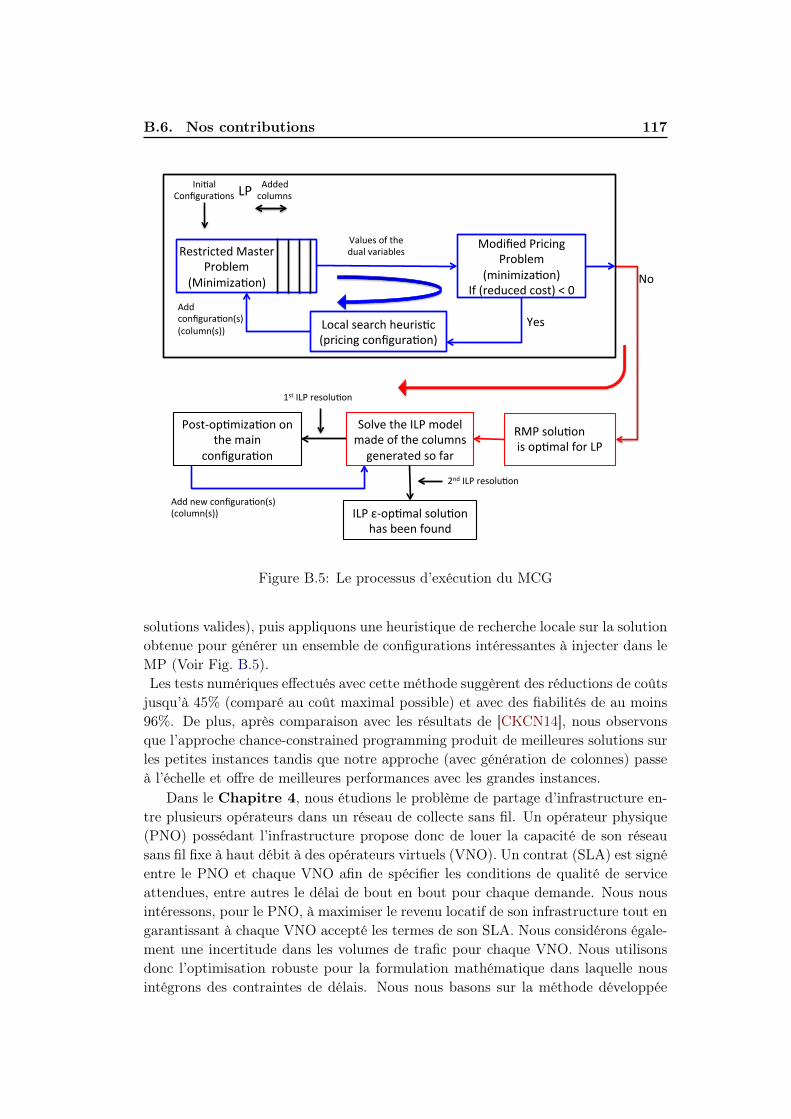
B.6. Nos contributions 117
Added columns LP Ini0al
Configura0ons
Modified Pricing Problem
(minimiza0on) If (reduced cost) < 0
Values of the dual variables
No
Restricted Master Problem
(Minimiza0on)
Yes Local search heuris0c (pricing configura0on)
Add configura0on(s) (column(s))
RMP solu0on is op0mal for LP
Solve the ILP model made of the columns generated so far
Post-‐op0miza0on on the main
configura0on
1st ILP resolu0on
ILP ε-‐op0mal solu0on has been found
2nd ILP resolu0on
Add new configura0on(s) (column(s))
Figure B.5: Le processus d’exécution du MCG
solutions valides), puis appliquons une heuristique de recherche locale sur la solutionobtenue pour générer un ensemble de configurations intéressantes à injecter dans leMP (Voir Fig. B.5).Les tests numériques effectués avec cette méthode suggèrent des réductions de coûtsjusqu’à 45% (comparé au coût maximal possible) et avec des fiabilités de au moins96%. De plus, après comparaison avec les résultats de [CKCN14], nous observonsque l’approche chance-constrained programming produit de meilleures solutions surles petites instances tandis que notre approche (avec génération de colonnes) passeà l’échelle et offre de meilleures performances avec les grandes instances.
Dans le Chapitre 4, nous étudions le problème de partage d’infrastructure en-tre plusieurs opérateurs dans un réseau de collecte sans fil. Un opérateur physique(PNO) possédant l’infrastructure propose donc de louer la capacité de son réseausans fil fixe à haut débit à des opérateurs virtuels (VNO). Un contrat (SLA) est signéentre le PNO et chaque VNO afin de spécifier les conditions de qualité de serviceattendues, entre autres le délai de bout en bout pour chaque demande. Nous nousintéressons, pour le PNO, à maximiser le revenu locatif de son infrastructure tout engarantissant à chaque VNO accepté les termes de son SLA. Nous considérons égale-ment une incertitude dans les volumes de trafic pour chaque VNO. Nous utilisonsdonc l’optimisation robuste pour la formulation mathématique dans laquelle nousintégrons des contraintes de délais. Nous nous basons sur la méthode développée
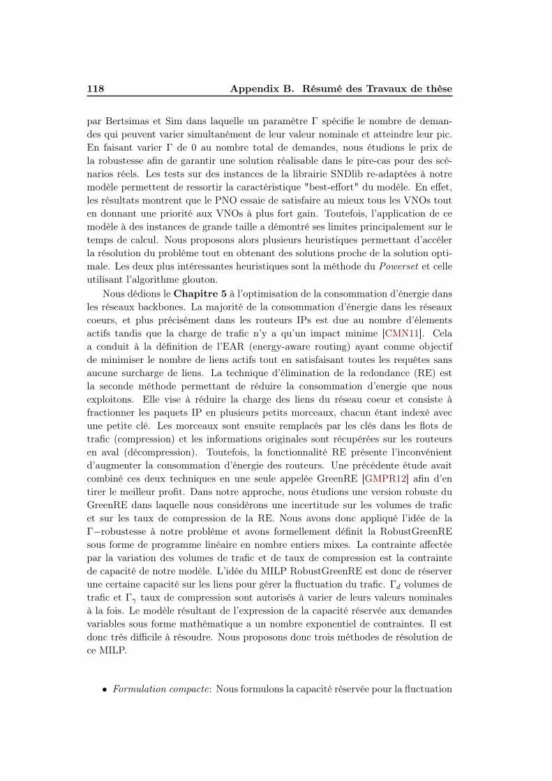
118 Appendix B. Résumé des Travaux de thèse
par Bertsimas et Sim dans laquelle un paramètre Γ spécifie le nombre de deman-des qui peuvent varier simultanément de leur valeur nominale et atteindre leur pic.En faisant varier Γ de 0 au nombre total de demandes, nous étudions le prix dela robustesse afin de garantir une solution réalisable dans le pire-cas pour des scé-narios réels. Les tests sur des instances de la librairie SNDlib re-adaptées à notremodèle permettent de ressortir la caractéristique "best-effort" du modèle. En effet,les résultats montrent que le PNO essaie de satisfaire au mieux tous les VNOs touten donnant une priorité aux VNOs à plus fort gain. Toutefois, l’application de cemodèle à des instances de grande taille a démontré ses limites principalement sur letemps de calcul. Nous proposons alors plusieurs heuristiques permettant d’accélerla résolution du problème tout en obtenant des solutions proche de la solution opti-male. Les deux plus intéressantes heuristiques sont la méthode du Powerset et celleutilisant l’algorithme glouton.
Nous dédions le Chapitre 5 à l’optimisation de la consommation d’énergie dansles réseaux backbones. La majorité de la consommation d’énergie dans les réseauxcoeurs, et plus précisément dans les routeurs IPs est due au nombre d’élementsactifs tandis que la charge de trafic n’y a qu’un impact minime [CMN11]. Celaa conduit à la définition de l’EAR (energy-aware routing) ayant comme objectifde minimiser le nombre de liens actifs tout en satisfaisant toutes les requêtes sansaucune surcharge de liens. La technique d’élimination de la redondance (RE) estla seconde méthode permettant de réduire la consommation d’energie que nousexploitons. Elle vise à réduire la charge des liens du réseau coeur et consiste àfractionner les paquets IP en plusieurs petits morceaux, chacun étant indexé avecune petite clé. Les morceaux sont ensuite remplacés par les clés dans les flots detrafic (compression) et les informations originales sont récupérées sur les routeursen aval (décompression). Toutefois, la fonctionnalité RE présente l’inconvénientd’augmenter la consommation d’énergie des routeurs. Une précédente étude avaitcombiné ces deux techniques en une seule appelée GreenRE [GMPR12] afin d’entirer le meilleur profit. Dans notre approche, nous étudions une version robuste duGreenRE dans laquelle nous considérons une incertitude sur les volumes de traficet sur les taux de compression de la RE. Nous avons donc appliqué l’idée de laΓ−robustesse à notre problème et avons formellement définit la RobustGreenREsous forme de programme linéaire en nombre entiers mixes. La contrainte affectéepar la variation des volumes de trafic et de taux de compression est la contraintede capacité de notre modèle. L’idée du MILP RobustGreenRE est donc de réserverune certaine capacité sur les liens pour gérer la fluctuation du trafic. Γd volumes detrafic et Γγ taux de compression sont autorisés à varier de leurs valeurs nominalesà la fois. Le modèle résultant de l’expression de la capacité réservée aux demandesvariables sous forme mathématique a un nombre exponentiel de contraintes. Il estdonc très difficile à résoudre. Nous proposons donc trois méthodes de résolution dece MILP.
• Formulation compacte: Nous formulons la capacité réservée pour la fluctuation
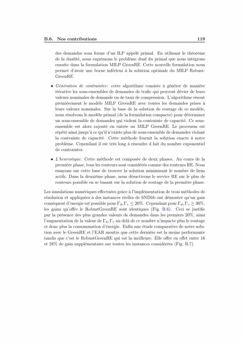
B.6. Nos contributions 119
des demandes sous forme d’un ILP appelé primal. En utilisant le théorèmede la dualité, nous exprimons le problème dual du primal que nous intégronsensuite dans la formulation MILP GreenRE. Cette nouvelle formulation nouspermet d’avoir une borne inférieur à la solution optimale du MILP Robust-GreenRE
• Génération de contraintes: cette algorithme consiste à générer de manièreitérative les sous-ensembles de demandes de trafic qui peuvent dévier de leursvaleurs nominales de demande ou de taux de compression. L’algorithme résoutpremièrement le modèle MILP GreenRE avec toutes les demandes prises àleurs valeurs nominales. Sur la base de la solution de routage de ce modèle,nous résolvons le modèle primal (de la formulation compacte) pour déterminerun sous-ensemble de demandes qui violent la contrainte de capacité. Ce sous-ensemble est alors rajouté en entrée au MILP GreenRE. Le processus estrépété ainsi jusqu’à ce qu’il n’existe plus de sous-ensemble de demandes violantla contrainte de capacité. Cette méthode fournit la solution exacte à notreproblème. Cependant il est très long à résoudre d fait du nombre exponentielde contraintes.
• L’heuristique: Cette méthode est composée de deux phases. Au cours de lapremière phase, tous les routeurs sont considérés comme des routeurs RE. Nousessayons sur cette base de trouver la solution minimisant le nombre de liensactifs. Dans la deuxième phase, nous désactivons le service RE sur le plus derouteurs possible en se basant sur la solution de routage de la première phase.
Les simulations numériques effectuées grâce à l’implémentation de trois méthodes derésolution et appliquées à des instances réelles de SNDlib ont démontré qu’un gainconséquent d’energie est possible pour Γd,Γγ ≤ 20%. Cependant pour Γd,Γγ ≥ 30%,les gains qu’offre le RobustGreenRE sont identiques (Fig. B.6). Ceci se justifiepar la présence des plus grandes valeurs de demandes dans les premiers 20%, ainsil’augmentation de la valeur de Γd,Γγ au delà de ce nombre n’impacte plus le routageet donc plus la consommation d’énergie. Enfin une étude comparative de notre solu-tion avec le GreenRE et l’EAR montre que cette dernière est la moins performantetandis que c’est le RobustGreenRE qui est la meilleure. Elle offre en effet entre 16et 28% de gain supplémentaire sur toutes les instances considérées (Fig. B.7).
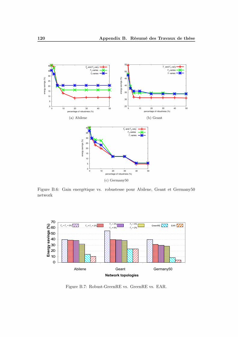
120 Appendix B. Résumé des Travaux de thèse
0
5
10
15
20
25
30
35
40
0 10 20 30 40 50
ener
gy s
avin
gs (%
)
percentage of robustness (%)
1
2
3
Гd varies
Г varies
Г and Гd vary
(a) Abilene
25
30
35
40
45
50
55
0 10 20 30 40 50
ener
gy s
avin
gs (%
)
percentage of robustness (%)
1
2
3
Г and Гd vary
Гd varies
Г varies
(b) Geant
0
5
10
15
20
25
30
35
40
0 10 20 30 40 50
ener
gy s
avin
gs (%
)
percentage of robustness (%)
1
2
3
Г and Гd vary
Гd varies
Г varies
(c) Germany50
Figure B.6: Gain energétique vs. robustesse pour Abilene, Geant et Germany50network
0
10
20
30
40
50
60
70
1 2 3
En
erg
y s
avin
gs (
%)
Network topologies
Abilene Geant Germany50
Гd = Гγ = 0% Гd = Гγ = 2%Гd = 2%
Гγ = 5%
Гd = 5%
Гγ = 2%GreenRE EAR
Figure B.7: Robust-GreenRE vs. GreenRE vs. EAR.
B.7. Liste des publications 121
B.7 Liste des publications
Nous présentons ici la liste des publications faisant objet de notre recherche.
[KJN+15] A. Kodjo, B. Jaumard, N. Nepomuceno, M. Kaddour, D. Coudert.Dimensionnement des réseaux de collecte de données sans fil par générationde colonnes In ROADEF, 2015, France.
[KJN+14] A. Kodjo, B. Jaumard, N. Nepomuceno, M. Kaddour, D. Coudert.Dimensioning microwave wireless networks, submitted to IEEE InternationalConference on Communications (ICC), 2015, UK.
[CKP14a] D. Coudert, A. Kodjo, and T.K. Phan. Robust Energy-aware Routingwith Redundancy Elimination, 2014 (Research report and Journal in revision).
[CKP14b] D. Coudert, A. Kodjo and T.K. Phan. Robust Optimization forEnergy-aware Routing with Redundancy Elimination In ALGOTEL 2014,France.
[KCCM14] A. Kodjo, D. Coudert and C. Caillouet-Molle. Optimisation robustepour le partage de reseaux d’acces micro-ondes entre operateurs In ROADEF,2014, France.
[CCK13] C. Caillouet-Molle, D. Coudert and A. Kodjo Robust optimization inmulti-operators microwave backhaul networks. In IEEE Global InformationInfrastructure and Networking Symposium (GIIS) 2013, Italy.
Cette thèse a été financée par la PME 3ROAM basée à Sophia Antipolis, et laprovince PACA.
B.8 Conclusion
Avec l’amélioration des technologies des réseaux d’accès permettant de fournir duhaut débit, le goulot d’étranglement du réseau de télécommunications est déplacévers le réseau de collecte. Tout au long de cette thèse, nous avons travaillé surplusieurs problèmes relatifs à l’utilisation des liaisons à micro ondes point à pointcomme technologie de transmission dans les réseaux de collecte. Notre principalobjectif était de minimiser les coûts de dimensionnement et d’exploitation de cettetechnologie.
Nous avons premièrement étudié le problème du dimensionnement à coût min-imal des réseaux sans fil fixes à haut débit dans des conditions non fiables. Nousavons proposé une solution basée sur le routage dynamique des demandes perme-ttant des réductions allant jusqu’à 45% du coût le plus élevé et des fiabilités d’aumoins 96% sur de larges réseaux. Notre solution présente également l’avantage depasser aisément à l’échelle pour des instances de grande taille.
122 Appendix B. Résumé des Travaux de thèse
Nous avons également abordé le concept des réseaux "verts" en utilisant la tech-nique du GreenRE pour réduire la consommation d’énergie des réseaux coeur. Nousavons significativement amélioré l’efficacité énergétique de ces réseaux grâce à notremodèle de RobustGreenRE. Nous avons également proposé une heuristique adaptéeà la résolution de ce problème sur de larges instances. Les résultats des simulationsdémontrent une amélioration en consommation d’énergie de l’ordre de 16 à 28%supplémentaire comparée à l’EAR.Enfin, grâce au partage de la capacité du réseau entre plusieurs opérateurs, nousavons proposé une solution intéressante aux détendeurs des réseaux de collectephysique pour améliorer leur revenue. Le modèle MILP formalisant ce problèmecombine les contraintes de routage des demandes, celles de qualité de service etde SLA. Plus encore, elle est robuste à la variation du volume de Γ demandes si-multanément. Due à sa lenteur de résolution sur de grandes instances, nous avonségalement proposé plusieurs heuristiques à ce problème.
En dépit des multiples résultats de notre thèse, plusieurs problèmes spécifiquesaux réseaux de collecte sans fil restent ouverts. Concernant le problème de dimen-sionnement, plusieurs améliorations algorithmiques devraient y être rajoutées afind’accélérer l’exécution de l’alogrithme de génération de colonnes et d’améliorer lafiabilité du réseau. Il existe également certains paramètres du problème que nousn’avons pas pu considérer dans notre modélisation. Il s’agit entre autres de lavariation du volume du trafic mais également de la corrélation existante entre lesconfigurations des liens à micro ondes. Une modélisation plus complète du problèmepourrait réduire davantage les coûts de dimensionnement pour les opérateurs.Une autre direction de recherche intéressante concerne le déploiement et l’extensionsur le long terme des réseaux de collecte. Les besoins en débit ne faisantqu’augmenter, les opérateurs auront besoin de recommandations sur quand et oùinstaller de nouveaux liens à micro ondes ou des liens à fibre optique ou quand ar-rêter l’utilisation d’un lien radio. Ceci soulève plusieurs problèmes d’optimisationdifficile à résoudre.Concernant l’efficacité energétique des réseaux de télécommunications, les opéra-teurs gagneraient à adapter aux réseaux de collecte les solutions proposées pour lesréseaux backbone. Il a été en effet prouvé que la consommation d’énergie des BScompte pour 50% de la consommation énergétique des réseaux d’accès. Avec la den-sification du déploiement des stations de base, l’efficacité energétique des réseauxde collecte deviendra assez rapidement un sujet de recherche très intéressant.
Enfin, nous complétons les travaux de notre thèse en nous intéressant àl’utilisation efficace du spectre radio. Nous avons dans ce sens démarré une étude,décrite dans l’Appendix A, sur le problème de partage de spectre dans les réseauxradio cognitifs (CRNs). Nous envisageons d’adapter le concept de la robustesseau problème de maximisation du débit des CRNs dans cet environnement haute-ment instable. Plusieurs problèmes intéressants restent également ouverts dans cedomaine de recherche.
Bibliography
[AAM11] G. Alnwaimi, K. Arshad, and K. Moessner, “Dynamic spectrum alloca-tion algorithm with interference management in co-existing networks,”IEEE Communications Letters, vol. 15, no. 9, pp. 932–934, 2011. (Citedin page 96.)
[AGA+08] A. Anand, A. Gupta, A. Akella, S. Seshan, and S. Shenker, “Packetcaches on routers: The implications of universal redundant traffic elim-ination,” SIGCOMM Computer Communication Review, vol. 38, no. 4,pp. 219–230, Aug. 2008. (Cited in pages 9, 64, 68, 80 and 114.)
[ALC09] I. F. Akyildiz, W.-Y. Lee, and K. R. Chowdhury, “Crahns: Cognitiveradio ad hoc networks,” Ad Hoc Networks, vol. 7, no. 5, pp. 810–836,2009. (Cited in page 94.)
[All08] N. Alliance, “NGMN optimised backhaul requirements,” Next Gener-ation Mobile Networks Alliance, p. 19, Aug. 2008. (Cited in pages 9and 114.)
[ALVM06] I. F. Akyildiz, W.-Y. Lee, M. C. Vuran, and S. Mohanty, “Next gen-eration/dynamic spectrum access/cognitive radio wireless networks: asurvey,” Computer Networks, vol. 50, no. 13, pp. 2127–2159, 2006.(Cited in pages x, 94 and 95.)
[AMAR09] A. Anand, C. Muthukrishnan, A. Akella, and R. Ramjee, “Redundancyin network traffic: Findings and implications,” in ACM InternationalJoint Conference on Measurement and Modeling of Computer Systems(SIGMETRICS). ACM, 2009, pp. 37–48. (Cited in pages 64, 68and 80.)
[ASA09] A. Anand, V. Sekar, and A. Akella, “SmartRE: An architecture forcoordinated network-wide redundancy elimination,” SIGCOMM Com-puter Communication Review, vol. 39, no. 4, pp. 87–98, Aug. 2009.(Cited in page 68.)
[AYP11] A. Altin, H. Yaman, and M. C. Pinar, “The robust network loadingproblem under hose demand uncertainty: formulation, polyhedral anal-ysis, and computations,” INFORMS Journal on Computing, vol. 23,no. 1, pp. 75–89, 2011. (Cited in page 17.)
[BAH+09] J. Baliga, R. Ayre, K. Hinton, W. V. Sorin, and R. S. Tucker, “Energyconsumption in optical ip networks,” IEEE/OSA Journal of LightwaveTechnology, vol. 27, no. 13, pp. 2391–2403, 2009. (Cited in pages 9and 114.)
124 Bibliography
[Bal86] M. O. Ball, “Computational complexity of network reliability analysis:An overview,” IEEE Transactions on Reliability, vol. 35, no. 3, pp.230–239, 1986. (Cited in page 25.)
[Bar72] W. T. Barnett, “Multipath propagation at 4, 6 and 11 GHz,” BellSystem Technical Journal, vol. 51, no. 2, pp. 311–361, 1972. (Cited inpage 24.)
[BBL08] S.-S. Byun, I. Balasingham, and X. Liang, “Dynamic spectrum alloca-tion in wireless cognitive sensor networks: Improving fairness and en-ergy efficiency,” in Vehicular Technology Conference, 2008. VTC 2008-Fall. IEEE 68th. IEEE, 2008, pp. 1–5. (Cited in page 96.)
[BCGT98] D. Bienstock, S. Chopra, O. Günlük, and C.-Y. Tsai, “Minimum costcapacity installation for multicommodity network flows,” Mathematicalprogramming, vol. 81, no. 2, pp. 177–199, 1998. (Cited in pages 7and 112.)
[BCL+10] A. P. Bianzino, C. Chaudet, F. Larroca, D. Rossi, and J. Rougier,“Energy-aware routing: A reality check,” in IEEE GLOBECOM Work-shop, Dec. 2010, pp. 1422–1427. (Cited in page 66.)
[BCRR12] A. P. Bianzino, C. Chaudet, D. Rossi, and J. Rougier, “A surveyof green networking research,” Communications Surveys & Tutorials,IEEE, vol. 14, no. 1, pp. 3–20, 2012. (Cited in pages 9 and 114.)
[BDB+11] R. Bolla, F. Davoli, R. Bruschi, K. Christensen, F. Cucchietti, andS. Singh, “The potential impact of green technologies in next-generationwireline networks: Is there room for energy saving optimization?”IEEE Communications Magazine, vol. 49, no. 8, pp. 80 – 86, Aug.2011. (Cited in page 64.)
[BHT11] J. Baliga, K. Hinton, and R. S. Tucker, Energy consumption of the In-ternet. University of Melbourne, Department of Electrical and Elec-tronic Engineering, 2011. (Cited in pages 9 and 114.)
[BJ88] T. B. Brecht and C. C. J., “Lower bounds on two-terminal networkreliability,” Discrete Applied Mathematics, vol. 21, no. 3, pp. 185–198,1988. (Cited in page 25.)
[Blu] “BlueCoat: WAN Optimization,” http://www.bluecoat.com/. (Citedin page 68.)
[BM04] M. R. Bussieck and A. Meeraus, “General algebraic modelingsystem (gams),” in Modeling languages in mathematical optimization.Springer, 2004, pp. 137–157. [Online]. Available: http://www.gams.com/ (Cited in page 20.)
Bibliography 125
[BS03] D. Bertsimas and M. Sim, “Robust discrete optimization and networkflows,” Mathematical Programming, vol. 98, no. 1-3, pp. 49 – 71, 2003.(Cited in pages 17 and 65.)
[BS04] ——, “The price of robustness,” Operations Research, vol. 52, no. 1,pp. 35–53, 2004. (Cited in pages 10, 17, 48, 49, 65 and 99.)
[BTEGN09] A. Ben-Tal, L. El Ghaoui, and A. Nemirovski, Robust optimization.Princeton University Press, 2009. (Cited in pages 17 and 99.)
[BTN00] A. Ben-Tal and A. Nemirovski, “Robust solutions of linear program-ming problems contaminated with uncertain data,” Mathematical pro-gramming, vol. 88, no. 3, pp. 411–424, 2000. (Cited in page 17.)
[BTN02] ——, “Robust optimization - methodology and application,” Mathe-matical Programming, vol. 92, pp. 453–480, 2002. (Cited in page 17.)
[BXG07] W. Bolton, Y. Xiao, and M. Guizani, “IEEE 802.20: mobile broadbandwireless access,” IEEE Wireless Communications, vol. 14, no. 1, pp.84–95, 2007. (Cited in pages 5 and 109.)
[CCK13] C. Caillouet, D. Coudert, and A. Kodjo, “Robust optimization in multi-operators microwave backhaul networks,” in Global Information Infras-tructure Symposium (GIIS). IEEE, 2013, pp. 1–6. (Cited in pages 10,12 and 121.)
[CCKN11a] G. Claßen, D. Coudert, A. Koster, and N. Nepomuceno, “Bandwidth as-signment for reliable fixed broadband wireless networks,” in 12th IEEEInternational Symposium on a World of Wireless Mobile and Multi-media Networks (WoWMoM), Jun. 2011, pp. 1–6. (Cited in pages 25and 44.)
[CCKN11b] ——, “A chance-constrained model & cutting planes for fixed broad-band wireless networks,” in International Network Optimization Con-ference (INOC), ser. Lecture Notes in Computer Science, vol. 6701,Hamburg, Germany, Jun. 2011, pp. 37–42. (Cited in pages 25 and 44.)
[CCLRP13] L. Chiaraviglio, A. Cianfrani, E. Le Rouzic, and M. Polverini, “Sleepmodes effectiveness in backbone networks with limited configurations,”Computer Networks, vol. 57, no. 15, pp. 2931–2948, 2013. (Cited inpage 67.)
[Chv83] V. Chvatal, Linear Programming. W. H. Freeman, 1983. (Cited inpage 49.)
[CKCN14] G. Claßen, A. M. Koster, D. Coudert, and N. Nepomuceno, “Chance-constrained optimization of reliable fixed broadband wireless net-works,” INFORMS Journal on Computing, vol. 26, no. 4, pp. 893–909,2014. (Cited in pages v, 10, 23, 25, 37, 40, 116 and 117.)
126 Bibliography
[CKP14a] D. Coudert, A. Kodjo, and K. Phan, “Robust energy-aware routingwith redundancy elimination,” Research Report RR-8457, Jan.2014. [Online]. Available: https://hal.inria.fr/hal-00936745 (Cited inpages 11 and 121.)
[CKP14b] ——, “Robust optimization for energy-aware routing with redundancyelimination,” in ALGOTEL 2014–16èmes Rencontres Francophones surles Aspects Algorithmiques des Télécommunications, 2014, pp. 1–4.(Cited in pages 11 and 121.)
[CKPT13] D. Coudert, A. M. Koster, T. K. Phan, and M. Tieves, “Robust re-dundancy elimination for energy-aware routing,” in Green Computingand Communications (GreenCom), 2013 IEEE and Internet of Things(iThings/CPSCom), IEEE International Conference on and IEEE Cy-ber, Physical and Social Computing. IEEE, 2013, pp. 179–186. (Citedin pages 9, 11, 18 and 65.)
[CKS13] G. Claßen, A. M. C. A. Koster, and A. Schmeink, “A robust optimi-sation model and cutting planes for the planning of energy-efficientwireless networks,” Computers and Operations Research, vol. 40, no. 1,pp. 80 – 90, 2013. (Cited in pages 18 and 65.)
[CLLC07] G. Cheng, W. Liu, Y. Li, and W. Cheng, “Spectrum aware on-demandrouting in cognitive radio networks,” in New Frontiers in DynamicSpectrum Access Networks, 2007. DySPAN 2007. 2nd IEEE Interna-tional Symposium on. IEEE, 2007, pp. 571–574. (Cited in page 96.)
[CMN09] L. Chiaraviglio, M. Mellia, and F. Neri, “Energy-aware backbone net-works: a case study,” in Communications Workshops, 2009. ICC Work-shops 2009. IEEE International Conference on. IEEE, 2009, pp. 1–5.(Cited in pages 9 and 114.)
[CMN11] ——, “Minimizing ISP network energy cost: Formulation and solu-tions,” IEEE/ACM Transaction in Networking, vol. 20, no. 2, pp. 463– 476, Apr. 2011. (Cited in pages 64, 67, 69, 70, 78 and 118.)
[CNR10] D. Coudert, N. Nepomuceno, and H. Rivano, “Power-efficient radioconfiguration in fixed broadband wireless networks,” ComputerCommunications, Special Section on Hot Topics in Mesh Networking,vol. 33, no. 8, pp. 898–906, May 2010. [Online]. Available:http://dx.doi.org/10.1016/j.comcom.2010.01.006 (Cited in page 24.)
[CNT11] D. Coudert, N. Nepomuceno, and I. Tahiri, “Energy saving in fixedwireless broadband networks,” in International Network OptimizationConference (INOC), ser. Lecture Notes in Computer Science, vol. 6701,Hamburg, Germany, Jun. 2011, pp. 484–489. (Cited in page 44.)
Bibliography 127
[CPP+08] K.-C. Chen, Y.-J. Peng, N. Prasad, Y.-C. Liang, and S. Sun, “Cog-nitive radio network architecture: part i–general structure,” in Pro-ceedings of the 2nd international conference on Ubiquitous informationmanagement and communication. ACM, 2008, pp. 114–119. (Citedin page 94.)
[Cra96] R. K. Crane, Electromagnetic wave propagation through rain. JohnWiley & Sons, 1996. (Cited in page 24.)
[CSB+08] J. Chabarek, J. Sommers, P. Barford, C. Estan, D. Tsiang, andS. Wright, “Power awareness in network design and routing,” in IEEEInternational Conference on Computer Communications (INFOCOM),Apr. 2008, pp. 1130–1138. (Cited in pages 9, 66 and 114.)
[DAB+02] A. Doufexi, S. Armour, M. Butler, A. Nix, D. Bull, J. McGeehan, andP. Karlsson, “A comparison of the HIPERLAN/2 and IEEE 802.11 awireless LAN standards,” Communications Magazine, IEEE, vol. 40,no. 5, pp. 172–180, 2002. (Cited in pages 4 and 109.)
[DBH+07] S. Dominiak, N. Bayer, J. Habermann, V. Rakocevic, and B. Xu, “Reli-ability analysis of IEEE 802.16 mesh networks,” in 2nd IEEE/IFIP In-ternational Workshop on Broadband Convergence Networks, BcN 2007,2007, pp. 1–12. (Cited in page 25.)
[DDS05] G. Desaulniers, J. Desrosiers, and M. M. Solomon, Column generation.Springer, 2005, vol. 5. (Cited in page 16.)
[DJ14] N. Dinh and V. Jeyakumar, “Farkas lemma: three decades of gener-alizations for mathematical optimization,” TOP, the official journalof the Spanish Society of Statistics and Operations Research, vol. 22,no. 1, pp. 1–22, 2014. (Cited in pages 19 and 100.)
[DL05] J. Desrosiers and M. E. Lübbecke, A primer in column generation.Springer, 2005. (Cited in page 16.)
[DVT08] N. Devroye, M. Vu, and V. Tarokh, “Cognitive radio networks,” SignalProcessing Magazine, IEEE, vol. 25, no. 6, pp. 12–23, 2008. (Cited inpage 94.)
[EGOL98] L. El Ghaoui, F. Oustry, and H. Lebret, “Robust solutions to uncertainsemidefinite programs,” SIAM Journal on Optimization, vol. 9, no. 1,pp. 33–52, 1998. (Cited in page 17.)
[FGK93] R. Fourer, D. Gay, and B. Kernighan, Ampl. Boyd & Fraser, 1993.(Cited in page 20.)
[GC97] A. Goldsmith and S.-G. Chua, “Variable-rate variable-power MQAMfor fading channels,” IEEE Transactions on Communications, vol. 45,pp. 1218–1230, 1997. (Cited in page 24.)
128 Bibliography
[GC98] ——, “Adaptive coded modulation for fading channels,” IEEE Trans-actions on Communications, vol. 46, no. 5, pp. 595–602, 1998. (Citedin page 24.)
[GC07] T. Grevers and J. Christner, Application Acceleration and WAN Op-timization Fundamentals, ser. Fundamentals series. Cisco Press, Jul.2007. (Cited in pages 68 and 70.)
[GCF99] B. Gendron, T. G. Crainic, and A. Frangioni, Multicommodity capaci-tated network design. Springer, 1999. (Cited in pages 7 and 112.)
[GGNS13] R. G. Garroppo, S. Giordano, G. Nencioni, and M. G. Scutellà, “Mixedinteger non-linear programming models for green network design,”Computers and Operations Research, vol. 40, no. 1, pp. 273–281, 2013.(Cited in page 67.)
[Glo07] “Global action plan,” http://globalactionplan.org.uk, 2007. (Cited inpage 64.)
[GMMO10] F. Giroire, D. Mazauric, J. Moulierac, and B. Onfroy, “Minimizingrouting energy consumption: from theoretical to practical results,” inIEEE/ACM Green Computing and Communications (GreenCom), Dec.2010, pp. 252–259. (Cited in pages 67 and 78.)
[GMPR12] F. Giroire, J. Moulierac, T. K. Phan, and F. Roudaut, “Minimizationof network power consumption with redundancy elimination,” in IFIPTC 6 International Conferences on Networking (NETWORKING), ser.Lecture Notes in Computer Science, vol. 7289. Springer, 2012, pp.247–258. (Cited in pages 9, 64, 67, 69, 70, 78 and 118.)
[GNTS13] R. G. Garroppo, G. Nencioni, L. Tavanti, and M. G. Scutellà, “Doestraffic consolidation always lead to network energy savings?” IEEECommunications Letters, vol. 17, no. 9, pp. 1852–1855, 2013. (Citedin page 67.)
[GS03] M. Gupta and S. Singh, “Greening of the Internet,” in ACM SpecialInterest Group on Data Communication (SIGCOMM). ACM, 2003,pp. 19–26. (Cited in page 64.)
[GSS+10] Y. Ge, J. Sun, S. Shao, L. Yang, and H. Zhu, “An improved spectrumallocation algorithm based on proportional fairness in cognitive radionetworks,” in Communication Technology (ICCT), 2010 12th IEEEInternational Conference on. IEEE, 2010, pp. 742–745. (Cited inpage 96.)
[HBF+11] K. Hinton, J. Baliga, M. Z. Feng, R. Ayre, and R. Tucker, “Powerconsumption and energy efficiency in the internet,” Network, IEEE,vol. 25, no. 2, pp. 6–12, 2011. (Cited in pages 9 and 114.)
Bibliography 129
[HEOL13] J. Hansryd, J. Edstam, B.-E. Olsson, and C. Larsson, “Non-line-of-sight microwave backhaul for small cells,” Ericsson Review, vol. 3, Feb.2013. (Cited in pages 3 and 107.)
[HGZD12] X. Huang, Y. J. Guo, A. Zhang, and V. Dyadyuk, “A multi-gigabit microwave backhaul,” Communications Magazine, IEEE,vol. 50, no. 3, pp. 122–129, 2012. [Online]. Available: http://ieeexplore.ieee.org/stamp/stamp.jsp?arnumber=6163591 (Cited inpages 3 and 107.)
[HLI07] A. T. Hoang, Y.-C. Liang, and M. Islam, “Maximizing throughput ofcognitive radio networks with limited primary users’ cooperation,” inCommunications, 2007. ICC’07. IEEE International Conference on.IEEE, 2007, pp. 5177–5182. (Cited in page 96.)
[HR09] Heavy-Reading, “Ethernet backhaul quartely market tracker,” HeavyReading Research, Tech. Rep., 2009. (Cited in pages ix, x, 3 and 107.)
[HR13a] ——. (2013, May) Converged microwave routers: Aheavy reading survey analysis. Report. Heavy Reading. [On-line]. Available: http://www.heavyreading.com/details.asp?sku_id=3147&skuitem_itemid=1547 (Cited in page 64.)
[HR13b] ——. (2013, September) Global mobile operator study on convergedmicrowave routers. Presentation. Aviat-Heavy reading. [Online]. Avail-able: http://www.aviatnetworks.com/media/files/HeavyReading_CMRReport_23Sep13.pdf (Cited in page 64.)
[IG] IEEE-GHN. Microwave link networks. News. IEEE Global HistoryNetwork. [Online]. Available: http://www.ieeeghn.org/wiki/index.php/Microwave_Link_Networks (Cited in page 5.)
[II14] IBM-ILOG. (2014) Cplex optimizer. IBM. [Online]. Avail-able: http://www-01.ibm.com/software/commerce/optimization/cplex-optimizer/ (Cited in pages 9, 21, 51, 80 and 115.)
[Joh99] M. Johnsson, “Hiperlan/2–the broadband radio transmission technol-ogy operating in the 5 ghz frequency band,” in HiperLAN/2 GlobalForum, vol. 2, 1999. (Cited in pages 4 and 109.)
[KAA09] Y. R. Kondareddy, N. Andrews, and P. Agrawal, “On the capacity ofsecondary users in a cognitive radio network,” in Sarnoff Symposium,2009. SARNOFF’09. IEEE. IEEE, 2009, pp. 1–5. (Cited in page 94.)
[KCCM14] A. Kodjo, D. Coudert, and C. Caillouet-Molle, “Optimisation robustepour le partage de réseaux d’accès micro-ondes entre opérateurs,” inROADEF-15ème congrès annuel de la Société française de recherche
130 Bibliography
opérationnelle et d’aide à la décision, 2014. (Cited in pages 10, 12and 121.)
[KJN+14] A. Kodjo, B. Jaumard, N. Nepomuceno, M. Kaddour, and D. Coudert,“Dimensioning microwave wireless networks,” 2014. (Cited in pages 10,11 and 121.)
[KJN+15] ——, “Dimensionnement des réseaux de collecte de données sans filpar génération de colonnes,” in ROADEF-16ème congrès annuel de laSociété française de recherche opérationnelle et d’aide à la décision,2015. (Cited in page 121.)
[KKR11] A. M. Koster, M. Kutschka, and C. Raack, “On the robustness of op-timal network designs,” in Communications (ICC), 2011 IEEE Inter-national Conference on. IEEE, 2011, pp. 1–5. (Cited in page 18.)
[KKR13] A. M. C. A. Koster, M. Kutschka, and C. Raack, “Robust networkdesign: Formulations, valid inequalities, and computations,” Networks,vol. 61, no. 2, pp. 128–149, 2013. (Cited in pages ix, 48, 49, 65, 76, 85and 89.)
[KPT13] A. M. C. A. Koster, T. K. Phan, and M. Tieves, “Extended cutsetinequalities for the network power consumption problem,” in Interna-tional Network Optimization Conference (INOC), ser. Electronic Notesin Discrete Mathematics, vol. 41. Elsevier, Jun. 2013, pp. 69–76.(Cited in page 80.)
[KT07] M. S. Kuran and T. Tugcu, “A survey on emerging broadband wirelessaccess technologies,” Computer Networks, vol. 51, no. 11, pp. 3013–3046, 2007. (Cited in pages 5 and 109.)
[Leh10] H. Lehpamer, Microwave Transmission Networks: Planning, Design,and Deployment, 2nd ed. New York: McGraw-Hill, 2010. (Cited inpages 6, 46 and 110.)
[LGL09] N. Li, L. Gong, and S. Li, “Price-based spectrum-allocation relay rout-ing in cognitive radio networks,” in Information, Communications andSignal Processing, 2009. ICICS 2009. 7th International Conference on.IEEE, 2009, pp. 1–5. (Cited in page 96.)
[LJJ10] D. H. Lee, W. S. Jeon, and D. G. Jeong, “Joint channel assignment androuting in cognitive radio-based wireless mesh networks,” in VehicularTechnology Conference (VTC 2010-Spring), 2010 IEEE 71st. IEEE,2010, pp. 1–5. (Cited in page 96.)
[LZ09] X. Li and S. A. R. Zekavat, “Distributed channel assignment in cogni-tive radio networks,” in Proceedings of the 2009 International Confer-ence on Wireless Communications and Mobile Computing: Connectingthe World Wirelessly. ACM, 2009, pp. 989–993. (Cited in page 96.)
Bibliography 131
[mar13] marketsandmarkets.com. (2013, November) Mobile and wirelessbackhaul market [by equipment (microwave, millimeter wave,sub 6 ghz, test and measurement), by services (network, sys-tem integration, professional)] - worldwide market forecasts andanalysis (2013 - 2018). Report. Market and Maerket. Forecastand analysis about mobile and wireless backhaul market (2013-2018). [Online]. Available: http://www.marketsandmarkets.com/Market-Reports/mobile-wireless-backhaul-market-1034.html (Citedin pages 3 and 107.)
[MCG09] I. Malanchini, M. Cesana, and N. Gatti, “On spectrum selection gamesin cognitive radio networks,” inGlobal Telecommunications Conference,2009. GLOBECOM 2009. IEEE. IEEE, 2009, pp. 1–7. (Cited inpage 96.)
[Min07] M. Minoux, “Duality, Robustness, and 2-stage robust LP decisionmodels. Application to Robust PERT Scheduling,” Annales duLAMSADE, Tech. Rep. 7, Oct. 2007. [Online]. Available: https://hal.archives-ouvertes.fr/hal-00180529 (Cited in pages 11, 17 and 18.)
[Min11] ——, “On 2-stage robust LP with RHS uncertainty: complexity resultsand applications,” Journal of Global Optimization, vol. 49, no. 3, pp.521–537, 2011. (Cited in pages 18, 99 and 100.)
[MYQ08] X. Mao, G. Yu, and P. Qiu, “On achievable rates and spectrum alloca-tion in cognitive wireless networks,” in Communications, Circuits andSystems, 2008. ICCCAS 2008. International Conference on. IEEE,2008, pp. 323–327. (Cited in page 96.)
[Nep10] N. Nepomuceno, “Network optimization for wireless microwavebackhaul,” Ph.D. dissertation, Ecole doctorale STIC, Universitéde Nice-Sophia Antipolis, Dec. 2010. [Online]. Available: http://tel.archives-ouvertes.fr/tel-00593412/ (Cited in pages 3, 6, 7, 107,110 and 113.)
[NIR+12] L. Niccolini, G. Iannaccone, S. Ratnasamy, J. Chandrashekar,and L. Rizzo, “Building a power-proportional software router,” inUSENIX Annual Technical Conference. Boston, MA, USA: USENIXAssociation, Jun. 2012, pp. 89–100. [Online]. Available: http://dl.acm.org/citation.cfm?id=2342821.2342829 (Cited in page 66.)
[Obs10] I. Observatory, “Spectrum and technology issues for mi-crowave backhaul in europe,” Innovation Observatory,Cambridge broadband networks, Tech. Rep., 2010. [On-line]. Available: http://cbnl.com/sites/all/files/userfiles/files/Spectrum-and-Technology-Issues-for-Microwave-Backhaul-in-Europe.pdf (Cited in pages ix, x, 4 and 108.)
132 Bibliography
[OWPT10] S. Orlowski, R. Wessäly, M. Pióro, and A. Tomaszewski, “SNDlib1.0 - survivable network design library,” Networks, vol. 55, no. 3,pp. 276–286, 2010. [Online]. Available: http://sndlib.zib.de (Cited inpages 9, 37, 50, 80 and 115.)
[Pea13] M. Peach. (2013, January) Nec and corning achieve petabitoptical transmission. Petabit optical transmission. [Online]. Available:http://optics.org/news/4/1/29 (Cited in page 2.)
[PVD+08] M. Pickavet, W. Vereecken, S. Demeyer, P. Audenaert, B. Vermeulen,C. Develder, D. Colle, B. Dhoedt, and P. Demeester, “Worldwide en-ergy needs for ict: The rise of power-aware networking,” in AdvancedNetworks and Telecommunication Systems, 2008. ANTS’08. 2nd In-ternational Symposium on. IEEE, 2008, pp. 1–3. (Cited in pages 8and 64.)
[PZZ06] C. Peng, H. Zheng, and B. Y. Zhao, “Utilization and fairness in spec-trum assignment for opportunistic spectrum access,” Mobile Networksand Applications, vol. 11, no. 4, pp. 555–576, 2006. (Cited in page 96.)
[RGM09] J. Restrepo, C. Gruber, and C. Machuca, “Energy profile aware rout-ing,” in IEEE International Conference on Communications – Work-shop on Green Communications, Jun. 2009, pp. 1–5. (Cited in page 66.)
[Riv] “Steelhead for WAN optimization,” http://www.riverbed.com/us/solutions/wan_optimization/. (Cited in page 68.)
[RM11] B. Raghavan and J. Ma, “The energy and emergy of the internet,” inProceedings of the 10th ACM Workshop on Hot Topics in Networks.ACM, 2011, p. 9. (Cited in pages 9 and 114.)
[SA11] B. Salameh and H. Ahmad, “Throughput-oriented channel assignmentfor opportunistic spectrum access networks,” Mathematical and Com-puter Modelling, vol. 53, no. 11, pp. 2108–2118, 2011. (Cited inpage 96.)
[SGG10] Y. Song, K. Guo, and L. Gao, “Redundancy-aware routing with limitedresources,” in International Conference on Computer Communicationsand Networks (ICCCN), Aug. 2010, pp. 1–6. (Cited in pages 64 and 68.)
[Soy73] A. L. Soyster, “Convex programming with set-inclusive constraintsand applications to inexact linear programming,” Operations research,vol. 21, no. 5, pp. 1154–1157, 1973. (Cited in pages 17, 18 and 99.)
[SW00] N. T. Spring and D. Wetherall, “A protocol-independent technique foreliminating redundant network traffic,” SIGCOMM Computer Com-munication Review, vol. 30, no. 4, pp. 87–95, Aug. 2000. (Cited inpage 68.)
Bibliography 133
[TBA+08] R. Tucker, J. Baliga, R. Ayre, K. Hinton, and W. Sorin, “Energy con-sumption in IP networks,” in ECOC Symposium on Green ICT, 2008,p. 1. (Cited in pages 9, 64 and 114.)
[TMF+14] S. Tombaz, P. Monti, F. Farias, M. Fiorani, L. Wosinska, and J. Zander,“Is backhaul becoming a bottleneck for green wireless access networks?”in Communications (ICC), 2014 IEEE International Conference on,June 2014, pp. 4029–4035. (Cited in page 92.)
[TMW+11] S. Tombaz, P. Monti, K. Wang, A. Vastberg, M. Forzati, and J. Zan-der, “Impact of backhauling power consumption on the deployment ofheterogeneous mobile networks,” in Global Telecommunications Con-ference (GLOBECOM 2011), 2011 IEEE. IEEE, 2011, pp. 1–5. (Citedin pages 8 and 114.)
[Tom66] J. Tomlin, “Minimum-cost multicommodity network flows,” OperationsResearch, vol. 14, no. 1, pp. 45–51, 1966. (Cited in pages 7 and 112.)
[TZFS13] E. Z. Tragos, S. Zeadally, A. G. Fragkiadakis, and V. A. Siris, “Spec-trum assignment in cognitive radio networks: A comprehensive sur-vey.” IEEE Communications Surveys and Tutorials, vol. 15, no. 3, pp.1108–1135, 2013. (Cited in pages 94 and 95.)
[TZJ11] O. Tipmongkolsilp, S. Zaghloul, and A. Jukan, “The evolution of cel-lular backhaul technologies: Current issues and future trends,” Com-munications Surveys Tutorials, IEEE, vol. 13, no. 1, pp. 97–113, First2011. (Cited in page 2.)
[Van05] F. Vanderbeck, “Implementing mixed integer column generation,” inColumn Generation. Springer, 2005, pp. 331–358. (Cited in page 16.)
[VH99] P. Van Hentenryck, The OPL Optimization Programming Language.Cambridge, MA, USA: MIT Press, 1999. (Cited in page 21.)
[VHIV+12] W. Van Heddeghem, F. Idzikowski, W. Vereecken, D. Colle, M. Pick-avet, and P. Demeester, “Power consumption modeling in optical mul-tilayer networks,” Photonic Network Communications, vol. 24, no. 2,pp. 86–102, 2012. (Cited in page 67.)
[Vig75] A. Vigants, “Space-diversity engineering,” Bell System Technical Jour-nal, vol. 54, no. 1, pp. 103–142, 1975. (Cited in pages 24 and 37.)
[VN10] S. J. Vaughan-Nichols, “Gigabit Wi-Fi is on its way,” Computer, vol. 43,no. 11, pp. 11–14, 2010. (Cited in pages 4 and 109.)
[WRL10] H. Wang, J. Ren, and T. Li, “Resource allocation with load balancingfor cognitive radio networks,” in Global Telecommunications Confer-ence (GLOBECOM 2010), 2010 IEEE. IEEE, 2010, pp. 1–5. (Citedin page 96.)
134 Bibliography
[YLH10] L. Yu, C. Liu, and W. Hu, “Spectrum allocation algorithm in cognitivead-hoc networks with high energy efficiency,” in Green Circuits andSystems (ICGCS), 2010 International Conference on. IEEE, 2010,pp. 349–354. (Cited in page 96.)
[ZA14] Y. Zhang and N. Ansari, “On protocol-independent data redundancyelimination,” Communications Surveys Tutorials, IEEE, vol. 16, no. 1,pp. 455–472, First 2014. (Cited in pages 9 and 114.)
[ZCM11] E. Zohar, I. Cidon, and O. O. Mokryn, “The power of prediction: Cloudbandwidth and cost reduction,” SIGCOMM Computer CommunicationReview, vol. 41, no. 4, pp. 86–97, Aug. 2011. (Cited in pages 9, 64, 68and 114.)
[ZYLZ10] M. Zhang, C. Yi, B. Liu, and B. Zhang, “GreenTE: Power-aware trafficengineering,” in IEEE International Conference on Network Protocols(ICNP), Oct. 2010, pp. 21–30. (Cited in page 64.)
Related Documents