DESIGN AND IMPLEMENTATION OF SEQUENCE DETECTION ALGORITHMS FOR DYNAMIC SPECTRUM ACCESS NETWORKS A Thesis Submitted to the Graduate School of the University of Notre Dame in Partial Fulfillment of the Requirements for the Degree of Master of Science in Electrical Engineering by Zhanwei Sun, J. Nicholas Laneman, Director Graduate Program in Electrical Engineering Notre Dame, Indiana April 2010

Welcome message from author
This document is posted to help you gain knowledge. Please leave a comment to let me know what you think about it! Share it to your friends and learn new things together.
Transcript

DESIGN AND IMPLEMENTATION OF SEQUENCE DETECTION
ALGORITHMS FOR DYNAMIC SPECTRUM ACCESS NETWORKS
A Thesis
Submitted to the Graduate School
of the University of Notre Dame
in Partial Fulfillment of the Requirements
for the Degree of
Master of Science
in
Electrical Engineering
by
Zhanwei Sun,
J. Nicholas Laneman, Director
Graduate Program in Electrical Engineering
Notre Dame, Indiana
April 2010

c© Copyright by
Zhanwei Sun
2010
All Rights Reserved

DESIGN AND IMPLEMENTATION OF SEQUENCE DETECTION
ALGORITHMS FOR DYNAMIC SPECTRUM ACCESS NETWORKS
Abstract
by
Zhanwei Sun
Spectrum sensing is a critical function for enabling dynamic spectrum access
(DSA) in a cognitive radio system. In DSA networks, unlicensed secondary users
can gain access to a licensed spectrum band as long as they do not cause harm-
ful interfere to the primary users. Although existing research has demonstrated
the utility of a Markov chain for modeling the spectrum access pattern of primary
users over time, little effort has been directed toward spectrum sensing based upon
such models. In this thesis, we develop several sequence detection algorithms for
spectrum sensing in DSA networks. We assign different costs for missed detections
and false alarms and show that a suitably modified forward-backward sequence
detection algorithm is optimal in minimizing the detection risk. Two advanced
sequence detection algorithms, the complete forward algorithm and the complete
forward partial backward algorithm are introduced. Along the way, we observe
new fundamental limitations that we call the risk floor and the window length
limitation of traditional physical layer detection schemes that arise from their
mismatch with the primary user’s channel access pattern. We also report re-
sults from preliminary experiments in which we implement and compare different
detectors using a software-defined radio platform.

To my family,
and my best friends,
those I love and those who love me.
ii

CONTENTS
FIGURES . . . . . . . . . . . . . . . . . . . . . . . . . . . . . . . . . . . . v
TABLES . . . . . . . . . . . . . . . . . . . . . . . . . . . . . . . . . . . . vii
ACKNOWLEDGMENTS . . . . . . . . . . . . . . . . . . . . . . . . . . . viii
CHAPTER 1: INTRODUCTION . . . . . . . . . . . . . . . . . . . . . . . 1
CHAPTER 2: BACKGROUND . . . . . . . . . . . . . . . . . . . . . . . . 52.1 Cognitive Radio and Dynamic Spectrum Access . . . . . . . . . . 52.2 Spectrum Sensing for Dynamic Spectrum Access . . . . . . . . . . 9
2.2.1 PHY Layer Sensing . . . . . . . . . . . . . . . . . . . . . . 102.2.2 Energy Detection . . . . . . . . . . . . . . . . . . . . . . . 122.2.3 MAC Layer Sensing . . . . . . . . . . . . . . . . . . . . . . 152.2.4 Cooperative Sensing . . . . . . . . . . . . . . . . . . . . . 17
2.3 Software-Defined Radio . . . . . . . . . . . . . . . . . . . . . . . . 192.3.1 Cognitive Radio and Software-Defined Radio . . . . . . . . 212.3.2 GNU Radio and USRP . . . . . . . . . . . . . . . . . . . . 22
CHAPTER 3: SEQUENCE DETECTION ALGORITHMS . . . . . . . . . 243.1 Hidden Markov Model in Spectrum Sensing . . . . . . . . . . . . 24
3.1.1 Markov Chain and Hidden Markov Model . . . . . . . . . 243.1.2 System Model . . . . . . . . . . . . . . . . . . . . . . . . . 26
3.2 Weighted Sequence Detection Algorithms . . . . . . . . . . . . . . 283.2.1 Impulse Sequence Cost and the Viterbi Algorithm . . . . . 293.2.2 Additive Sequence Cost and the Forward-Backward Algorithm 313.2.2.1 Forward Probabilities . . . . . . . . . . . . . . . . . . . 333.2.2.2 Backward Probabilities . . . . . . . . . . . . . . . . . . . 333.2.2.3 A Posterior Probability of an Individual Symbol . . . . . 35
3.3 Overlapping and Non-Overlapping Sensing Rules . . . . . . . . . 373.4 Comparison to Energy and Coherent Detection . . . . . . . . . . 39
iii
3.4.1 Threshold for Energy Detection and Coherent Detection . 413.4.2 Risk Floor For Energy Detection . . . . . . . . . . . . . . 44
CHAPTER 4: NUMERICAL RESULTS . . . . . . . . . . . . . . . . . . . 484.1 Sequence Detection versus Energy and Coherent Detection . . . . 484.2 CFA versus CFPB . . . . . . . . . . . . . . . . . . . . . . . . . . 514.3 Risk Floor for Energy Detection . . . . . . . . . . . . . . . . . . . 52
CHAPTER 5: IMPLEMENTATION OF ENERGY DETECTION ANDSEQUENCE DETECTION ALGORITHMS . . . . . . . . . . . . . . . 575.1 Experimental Setup and System Parameters . . . . . . . . . . . . 575.2 Primary Transmission . . . . . . . . . . . . . . . . . . . . . . . . 59
5.2.1 Transmission Parameters . . . . . . . . . . . . . . . . . . . 595.2.2 Primary User’s Channel Access Structure . . . . . . . . . . 60
5.3 Spectrum Analysis, Modeling and Learning by Secondary User . . 625.3.1 SU in PROBING State . . . . . . . . . . . . . . . . . . . . 665.3.2 SU in TRACKING State . . . . . . . . . . . . . . . . . . . 705.3.3 SU in SENSING State . . . . . . . . . . . . . . . . . . . . 72
5.4 Implementation of Energy Detection . . . . . . . . . . . . . . . . 725.5 Implementation of Sequence Detection . . . . . . . . . . . . . . . 735.6 Practical Issues . . . . . . . . . . . . . . . . . . . . . . . . . . . . 83
5.6.1 USRP Limitations . . . . . . . . . . . . . . . . . . . . . . 835.6.1.1 Switch Time . . . . . . . . . . . . . . . . . . . . . . . . 835.6.1.2 USRP Overrun . . . . . . . . . . . . . . . . . . . . . . . 845.6.1.3 Sampling Offset . . . . . . . . . . . . . . . . . . . . . . . 845.6.2 Deviation of Real World from Ideal Modeling . . . . . . . 865.6.2.1 Imperfect Estimation . . . . . . . . . . . . . . . . . . . . 865.6.2.2 Bursty Interference From Unknown Sources . . . . . . . 875.6.2.3 Variation in Noise and Channel Fading . . . . . . . . . . 87
CHAPTER 6: CONCLUSIONS AND FUTURE WORK . . . . . . . . . . 88
BIBLIOGRAPHY . . . . . . . . . . . . . . . . . . . . . . . . . . . . . . . 91
iv
FIGURES
1.1 Real world spectrum usage measurements averaged over six locations. 2
2.1 Illustration of dynamic spectrum access network. . . . . . . . . . 6
2.2 Cognitive radio circle . . . . . . . . . . . . . . . . . . . . . . . . . 8
2.3 Two realizations of energy detection. a) Implementation with ana-log pre-filter and square-law device. b) Implementation using FFTmagnitude squared and averaging . . . . . . . . . . . . . . . . . . 13
2.4 Typical TX and RX path for a software radio . . . . . . . . . . . 22
3.1 Hidden Markov Model . . . . . . . . . . . . . . . . . . . . . . . . 28
3.2 Forward and backward procedure. . . . . . . . . . . . . . . . . . . 34
3.3 Non-overlapping (block) rule. . . . . . . . . . . . . . . . . . . . . 37
3.4 Overlapping (sliding) rule. . . . . . . . . . . . . . . . . . . . . . . 38
3.5 Complete forward algorithm (CFA) and complete forward partialbackward (CFPB). . . . . . . . . . . . . . . . . . . . . . . . . . . 39
3.6 Two cases leading to false alarms for energy detection when the PUstate changes during a sensing window. . . . . . . . . . . . . . . . 46
4.1 Detection performance and sensing window length. E[L0] = 2000,E[L1] = 1000, SNR=-10dB, P f = 0.1, C01 = 1, C10 = 1. . . . . . . 49
4.2 Receiving Operating Characteristics. E[L0] = 100, E[L1] = 50,SNR=-10dB, C01 = 1, C10 = 1. . . . . . . . . . . . . . . . . . . . 52
4.3 Performance for CFA and CFPB. E[L0] = 200, E[L1] = 100, C01 =10, C10 = 1. . . . . . . . . . . . . . . . . . . . . . . . . . . . . . . 53
4.4 Performance for CFA and CFPB. E[L0] = 200, E[L1] = 100, C01 =10, C10 = 1. . . . . . . . . . . . . . . . . . . . . . . . . . . . . . . 54
4.5 The risk floor for energy detection. E[L0] = 2000, E[L1] = 1000,T = 10, C01 = 10, C10 = 1. . . . . . . . . . . . . . . . . . . . . . . 55
v

4.6 The risk floor for energy detection. E[L0] = 2000, E[L1] = 1000,T = 100, C01 = 10, C10 = 1. . . . . . . . . . . . . . . . . . . . . . 56
5.1 Packet format. . . . . . . . . . . . . . . . . . . . . . . . . . . . . . 60
5.2 Pilot structure and half-pilot-size sensing window. . . . . . . . . . 61
5.3 PU’s channel access structure. . . . . . . . . . . . . . . . . . . . . 62
5.4 Flow graph of the self-adaptive cognitive spectrum sensing engine. 65
5.5 Correlator for half-pilot-size power estimator. . . . . . . . . . . . 68
5.6 Two matched patterns in the TRACKING mode . . . . . . . . . . 71
5.7 Risk level for energy detectors with different sensing window length. 74
5.8 System setup. . . . . . . . . . . . . . . . . . . . . . . . . . . . . . 75
5.9 Noise power and its histogram in a wireless environment. . . . . . 76
5.10 Received signal power and its histogram in a wireless environment. 77
5.11 Noise power and its histogram in a wired environment. . . . . . . 78
5.12 Received signal power and its histogram in a wired environment. . 79
5.13 Divide a sensing window into several subwindows . . . . . . . . . 80
5.14 Estimated detection risks of energy detection, complete forward se-quence detection algorithm and complete forward partial backwardsequence detection algorithm. . . . . . . . . . . . . . . . . . . . . 82
5.15 Sampling frequency offset causes pattern mismatch and estimationerrors. . . . . . . . . . . . . . . . . . . . . . . . . . . . . . . . . . 85
vi

TABLES
5.1 Implementation parameters for wireless system . . . . . . . . . . 63
5.2 Implementation parameters for the calibrated wired system . . . 80
vii

ACKNOWLEDGMENTS
On writing the thesis, I would like to express my sincere gratitude and thanks
to my advisor Dr. J. Nicholas Laneman for his support and guidance in research,
help and patience in life. Not only did I learn a lot from discussion with him, but
he helped me overcome some difficult time in life. He is a great life coach and
friend as he is an academic advisor!
Many thanks should go to Glenn Bradford, for his constant help in the exper-
imentation and others as well. Without his help, this thesis could not have been
done. I would also like to thank Ioannis Krikidis, Michael Dickens, Brian Dunn,
Matthieu Bloch, Ebrahim MolavianJazi and Utsaw Kumar, since I benefit a lot
from interacting with these group members.
Special thanks go to Ke Chen, for his cares and willingness to help in this
process, and to Yaou Zhou, for her thoughtful help and encouragement during the
hard time. Thank Ke Lang and Jun Geng for caring, understanding, support-
ing and valuing me and being my best friends for more than ten years! Thank
Fangxue Zheng, Xian Jiang, Ming Gan, Xiao Fang, Xue Xiao, Yuan Liu, Yuzhe
Liu, Zhisheng Lin and Li Yu. Your friendship makes my life in US exciting and
memorable! Thank my US brother John Bales and his wife Holly Bales for hosting
me and making me feel at home. Their love and support means a lot to me.
Aboveall, thank my parents. Your love is the greatest gift in my life!
viii

CHAPTER 1
INTRODUCTION
Though the natural frequency spectrum is a limited resource, the demand for
extra spectrum is ever increasing with the rapid growth of wireless applications and
services. In the current spectrum regulatory framework, all the frequency bands
are exclusively allocated to specific services by governmental regulators. However,
the actual licensed spectrum is spectrally inefficient due to spatial and temporal
variation in utilization by licensed primary users (PUs). One report of the Federal
Communications Commission (FCC) suggests that the utilization of allocated
spectrum ranges from 15% to 85% [9]. In [4], the authors provide real world
spectrum usage measurements averaged over six locations and the result is shown
in Figure [? ]. Cognitive Radio (CR) and Dynamic spectrum access (DSA) [3, 32]
are promising approaches to spectrum scarcity problem by allowing unlicensed,
secondary users (SUs) to opportunistically access the inefficiently used licensed
spectrum as long as they do not cause harmful interference to PUs. SUs employing
DSA must accurately sense spectrum opportunities, often called spectrum holes,
corresponding to gaps in PU transmissions.
Spectrum sensing algorithms seek to balance the conflicting goals of minimizing
interference to PUs while maximizing the rate of SUs. Performance of a sensing
algorithm is typically characterized in terms of the probability of missed detection
Pm, i.e., failing to sense the existence of an active PU and thus causing interference,
1

Figure 1.1. Real world spectrum usage measurements averaged over sixlocations.
2
and the probability of false alarm Pf , i.e., falsely declaring that a PU is active
and thus missing a spectrum opportunity. The inherent tradeoff between Pm
and Pf for any detector leads to a tradeoff between these two aspects of system
performance.
Spectrum sensing is best addressed as a cross-layer design problem. Various
types of physical (PHY) layer, medium access control (MAC) layer, and cross-
layer sensing approaches exist in the literature. However, few of them take into
consideration the PUs’ channel access pattern. Instead, they typically assume
that PUs remain in one state during a sensing period, regardless of the length
of a sensing window. Classical PHY layer spectrum sensing approaches for a
non-cooperating SU, such as coherent and energy detection [5], generally assume
that any operating pair (Pf , Pm) is achievable at a given signal-to-noise ratio
(SNR) as long as a suitably long observation window is allowed. But in practice,
a PU’s access pattern is likely to be bursty, and not staying in one state for
long. Therefore, the observation length, and thus performance of these classical
approaches, will be limited by the PU’s channel dwell time, which refers to the
time duration that the PU remains in a particular state, whether ON or OFF.
This type of bursty transmission can be modeled as a Markov Chain [14] and
recent real-time measurements collected in the paging band (928-948 MHz) also
validates its appropriateness [7].
The primary contribution of this thesis is to develop several sequence detection
algorithms derived from the well-known forward-backward algorithm and apply
them to the problem of spectrum sensing in cognitive radio networks. These se-
quence detection algorithms outperform the classical PHY layer sensing schemes
by fully exploiting the Markov memory modeling the PU’s channel access pat-
3

tern. Furthermore, by assigning different cost factors for missed detections and
false alarms, the proposed sequence detection algorithms allow for operation at
different (Pf , Pm) pairs. Comparisons among energy detection and the proposed
sequence detection algorithms are provided using theory, simulations, and prelim-
inary experiments on a software radio platform. Along the way, new limitations
for classical PHY layer sensing schemes are characterized.
The remainder of this thesis is organized as follows. Chapter 2 provides back-
ground on cognitive radio and software radio, focusing on algorithms for spectrum
sensing and the GNU radio platform used for experiments, respectively. Chapter 3
describes the proposed weighted sequence detection algorithms for spectrum sens-
ing. It also describes some limitations for traditional PHY layer sensing schemes.
Chapter 4 provides some simulation results, which show the advantage of the new
sequence detection algorithms over the energy detection and coherent detection.
Chapter 5 describes an experimental setup for implementing energy detection and
the proposed sequence detection algorithms. A simplified version of the sequence
detection algorithms is implemented and several experimental results are provided.
Chapter 6 concludes the thesis and discusses directions for future research.
4

CHAPTER 2
BACKGROUND
This chapter gives a survey of relevant literature and techniques on cognitive
radio (CR) and software-defined radio (SDR). Specifically, Section 2.1 introduces
the definition of cognitive radio and dynamic spectrum access (DSA). Section 2.2
provides a thorough exploration of different spectrum sensing schemes. Section 2.3
introduces SDR and the the implementation platform for this thesis, the GNU
Radio software and the Universal Software Radio Peripheral (USRP) hardware.
2.1 Cognitive Radio and Dynamic Spectrum Access
Cognitive radio and dynamic spectrum access techniques are new communica-
tion paradigms that can offer new ways of exploiting the underutilized spectrum.
There is often confusion about these two terms and very often they are used in-
terchangeably. In fact, cognitive radio is a much broader paradigm. The term
cognitive radio is promoted by Mitola[2]. It is a context-aware intelligent radio
potentially capable of autonomous reconfiguration by learning from and adapting
to the communication environment. Dynamic spectrum access, however, corre-
sponds to a narrower paradigm which stands for the opposite of the current static
spectrum management policy. The basic idea of dynamic spectrum access is to
allow secondary users (also called unlicensed users) to access licensed spectrum
5

Figure 2.1. Illustration of dynamic spectrum access network.
bands as long as they do not cause any harmful interference to primary users (also
called licensed users). Hence, dynamic spectrum access can be viewed as a subset
of cognitive radio.
Figure 2.1 illustrates a simple, yet typical dynamic spectrum access network
that consists of a pair of primary user and a pair of secondary user. They operate
at exactly the same frequency band. The primary user has higher priority access-
ing the spectrum. The secondary user has to sense the spectrum and transmit
only if it detects a spectrum hole. Miss detections from the secondary user will
cause interference to the primary user as shown in the figure.
Strictly speaking, there is no agreement on the formal definition of cognitive
radio as for now. The concept of ultimate cognitive radio should include vari-
6

ous meanings in several contexts. One main aspect is to exploit locally unused
spectrum to provide opportunistic spectrum access. Other aspects include inter-
operability across several networks, roaming across borders while being able to
stay in compliance with local regulations, adapting the system, transmission, and
reception parameters without user intervention, and having the ability to under-
stand and follow actions and choices taken by their users to learn how to become
more responsive over time.
In [1], cognitive radio is defined as an intelligent wireless communication sys-
tem that is aware of its surrounding environment and uses the methodology of
understanding-by-building to learn from the environment and adapt its internal
states to statistical variations in the incoming RF stimuli by making corresponding
changes in certain operating parameters (e.g., transmit-power, carrier-frequency,
and modulation strategy) in real-time.
Figure 2.1 shows the tasks required for cognitive radio in open spectrum. It
is referred to as the cognitive cycle [1], [20]. In the spectrum analysis, modeling
and learning step, the cognitive radio measures the spectrum, estimates the PU’s
transmission parameters and models the PU’s transmission structure through ob-
servations over a long time period. This information is then used to formulate the
threshold in the spectrum sensing, channel predication step. Finally, in the spec-
trum management, cognitive transmission step, the cognitive radio adapts itself
to transmit in the open band, potentially changing its carrier frequency, transmit
power, modulation type and packet length. If multiple SUs exist, they must share
the spectrum according to some channel access protocol.
7

Radio environment:Primary users and
other secondary users
Spectrum analysis
channel prediction
cognitive transmission modeling, and learning
Spectrum sensing,
RF stimuli
RF stimuli
Spectrum management,Spectrum holes and
noise statistics
Spectrum holes andnoise statistics
channel capacity
Channel allocation,power and packetlength control
information
Figure 2.2. Cognitive radio circle
8

2.2 Spectrum Sensing for Dynamic Spectrum Access
Spectrum sensing by far is the most important task for the establishment of
cognitive radio and dynamic spectrum access. Traditionally, spectrum sensing
is understood as measuring the spectrum to decide whether PUs are active or
not, but if the ultimate cognitive radio is considered, it is a more general term
that may involve obtaining the spectrum usage characteristics across multiple
dimensions such as time, space, frequency, and code, as well as determining what
type of signals are occupying the spectrum, i.e., modulation scheme, waveform,
bandwidth, carrier frequency, etc. This will of course require more powerful signal
analysis techniques with additional computational complexity. For the purpose of
this thesis, we only consider the spectrum sensing in the traditional sense.
Detection of the presence of primary users should be in such a way that the
probability of missed detection Pm and the probability of false alarm Pf , should
not exceed a certain levels, because Pf and Pm have unique implications for cogni-
tive networks. Small Pf is necessary in order to provide possible high throughput
in dynamic spectrum access networks, since a false alarm wastes a spectrum oppor-
tunity. On the other hand, small Pm is necessary in order to limit the interference
from SUs to PUs.
Spectrum sensing schemes may be reactive or proactive according to the way
they search for white spaces. Reactive schemes are energy efficient, operate on
an on-demand basis in which a SU starts to sense the spectrum only when it has
some data to transmit. Proactive schemes, on the other hand, aim at minimizing
the delay incurred by secondary users in finding an idle spectrum by maintaining
a list of one or more licensed channels currently available for opportunistic access
through periodic sensing of the spectrum. It is noteworthy that while a SU is
9

utilizing a white space, it no longer has a choice regarding the sensing mode and
has to sense the channel proactively at periodic intervals since it needs to vacate
its transmission as soon as any primary users reclaim that channel [4]. Therefore,
the application characteristics may prevent a SU with a reactive sensing scheme
from joining in the cooperation.
Spectrum sensing can be realized as a two-layer mechanism [8]. PHY layer
sensing focuses on efficiently detecting PU signals. Several well-known PHY layer
detection methods such as energy detection, coherent detection, and feature de-
tection have been extensively investigated [5], [6], [9], [10]. On the other hand,
MAC layer sensing determines when SUs have to sense which channels and for
how long.
2.2.1 PHY Layer Sensing
PHY layer sensing focuses on how to detect the presence of primary signals
rapidly and robustly. It is accomplished by using or not using the parameters of
the primary signals such as transmission power, waveform, modulation schemes.
The most well-known PHY layer sensing schemes include energy detection (power
detection, periodogram detection), coherent detection (matched filter detection)
and feature detection (cyclostationary detection). Because of its computational
and implementation simplicity and good performance in practice, we will discuss
energy detection in more detail in Section 2.2.2. For now we will focus on other
PHY layer sensing schemes.
Coherent detection using a matched filter would be ideal for spectrum sensing
since it maximizes received signal-to-noise ratio. In practice, coherent detection is
often applied to known pilot signals. However, coherent detection requires a priori
10

knowledge of primary signal at both PHY and MAC layers, such as modulation
scheme, pulse shape and packet format. Moreover, for demodulation it has to be
synchronized with primary signal in timing and carrier frequency [9]. Therefore,
it is very vulnerable to uncertainty and changes in the primary signal and the
timing and frequency offset. Furthermore, a different detector is required in order
to detect each PU (or other SUs in the same cognitive radio system). This makes
coherent detection undesirable if multiple primary systems are to be sensed.
By definition in [22], a cyclostationary signature is a feature, intentionally em-
bedded in the physical properties of a digital communications signal, which may
be easily generated, manipulated, detected and analyzed using low complexity
transceiver architectures. This feature is present in most transmitted signals, re-
quires little signaling overhead, and may be detected using short signal observation
times. Cyclostationary signatures are an effective tool for overcoming a number
of the principal challenges associated with cognitive network and dynamic spec-
trum access applications. By taking advantage of the inherent cyclostationarity
existent in digital signals, feature detection has the potential to provide reliable
signal classification even at low SNR [23]. Feature detection outperforms energy
detection by exploiting an inherent periodicity in the primary users’ signal. How-
ever, cyclostationary detection’s improved performance is at the cost of increased
complexity.
In [24], the author proposed a blind sensing algorithm based on oversampling
the received signal. The proposed algorithm uses a novel combination of oblique
projection and QR decomposition based approach to handle bandlimited signals.
This algorithm does not require any a priori knowledge of the primary signal or
the channel and noise power. In fact, the estimation is just involved in two signal
11

statistics based on the oblique projection operator. One signal statistic provides
an estimate of the primary signal present in the received data. The other signal
statistic provides an estimate of the noise variance, even if the received signal
contains both signal and noise.
Other blind sensing methods are based on the eigenvalues of the covariance
matrix of the received signal [25]. The Maximum-Minimum Eigenvalue (MME)
detection algorithm is based on the ratio of the maximum eigenvalue to minimum
eigenvalue, and the Energy with Minimum Eigenvalue (EME) detection algorithm
is based on the ratio of average power of the received signal to the minimum
eigenvalue.
Similar to energy detection, both MME and EME are blind detection methods
that only use the received signal samples but limited information on the trans-
mitted signal and channel. MME and EME outperform energy detection in two
ways. First, energy detection needs the noise power for decision while MME and
EME do not. In fact, estimation of noise power is naturally embedded in these
methods. As a result, MME and EME are robust to noise uncertainty and varia-
tion. Second, MME and EME also provide better performance if the signal to be
detected are highly correlated [25]. Of course, these advantages are at the cost of
increased complexity.
2.2.2 Energy Detection
Energy detection has been widely applied since it requires limited a priori
knowledge of primary signals to be detected. It is also one of the lowest complexity
schemes.
In the simplest form, the spectrum sensing problem at a given interval of time
12

A/D Average Nsamples
y(t)
test statistic
Comparator sensingresult
A/Dy(t)
test statistic
Comparator sensingresultFFT | |2
| |2
bins N timesAverage M
(a)
(b)
Figure 2.3. Two realizations of energy detection. a) Implementationwith analog pre-filter and square-law device. b) Implementation using
FFT magnitude squared and averaging
can be formulated as a binary hypothesis testing problem to distinguish between:
H0 : Yt = Wt, t = 1, 2, ..., T, signal absent
H1 : Yt = Xt +Wt, t = 1, 2, ..., T, signal present (2.1)
where T is the observation length. The test statistic for an energy detector is
Z(y) =T∑t=1
|Yt|2 (2.2)
This statistic is compared with a predetermined threshold ε. If Z > ε, signal
presence is declared, and if Z < ε, signal absence is declared. Figure 2.2.2 shows
two realizations of an energy detector. Note that although these two types are
basically the same by Parseval’s theorem, the second type is sometimes referred
to as periodogram detection.
13

The noise samples Wt are assumed to be additive, white and Gaussian with
zero mean and variance σ2w. For a simplified analysis, the signal samples Xt can
also be modeled as uncorrelated zero mean Gaussian random process with variance
σ2x [5]. Based on these assumptions, the decision statistic Z follows central chi-
square distribution with 2T degrees of freedom under H0 and non-central chi-
square distribution with 2T degrees of freedom and a non-central parameter of 2γ
under H1 [28], i.e.,
Z ∼
χ2
2T , H0,
χ22T (2γ), H1.
(2.3)
where γ = σ2w/σ
2x is the signal-to-noise-ratio.
For large T , the above chi-square distribution can be approximated by a Gaus-
sian distribution. If the number of samples used in a sensing window is not limited,
an energy detector can meet any desired Pd and Pf simultaneously. The minimum
number of samples for a prescribed Pd and Pf is given by [5]
T = 2
[(Q−1(Pf )−Q−1(Pd)
)γ−1 −Q−1(Pd)
]2
(2.4)
The well-known limitation for energy detection is the SNR wall caused by
uncertainties in background noise power [6]. SNR Wall is the smallest power
under which the signal cannot be detected. Energy detection relies on accurate
knowledge of the noise power. The threshold for energy detection is based on the
assumption that the noise variance is known precisely to the receiver. However,
this is impossible in practice since noise might vary over time due to factors
such as interference of nearby unintentional transmissions and far-away intentional
transmissions, as well as non-uniform and time varying thermal noise. Other
14

challenges with energy detection include selection of the threshold and inability
to detect spread spectrum signals.
2.2.3 MAC Layer Sensing
MAC layer sensing concentrates on how to schedule sensing for efficient dis-
covery of spectrum opportunities, especially in the case of multiple channels and
multiple SUs. Important issues associated with MAC layer sensing in dynamic
spectrum access networks are how often to sense the availability of licensed chan-
nels, in which order to sense, and how long a sensing period should be. Recently,
significant effort has been devoted to the field of MAC layer sensing and scheduling
[8, 11–14].
In [14], the authors propose an analytical framework for opportunistic spec-
trum access based on the theory of partially observable Markov decision process
(POMDP). This decision-theoretic approach integrates the design of spectrum ac-
cess protocols at the MAC layer with spectrum sensing at the physical layer and
traffic statistics determined by the application layer of the primary network. It
can easily incorporate sensing error and collision constraint on the primary users.
The proposed MAC protocols optimize the performance of SUs while limiting the
interference to the primary users under the POMDP framework. A suboptimal
strategy with reduced complexity yet comparable performance is also developed.
In [11], the authors propose a joint channel sensing and transmission strategy
in multichannel systems to maximize SU performance by intelligently deciding
the sequence of channel probing/sensing and optimal action on each channel. The
authors consider a cognitive transmitter with multiple licensed channels of known
state distributions and channel-dependent costs. The scheme seeks to decide which
15

channels to probe, in what order, when to stop, and upon stopping, which channel
to use before each cognitive transmission starts. The optimal strategy is shown
to have a threshold structure.
In [8], the authors address the issue of how to maximize the discovery of spec-
trum opportunities by sensing-period adaptation and how to minimize the delay
in finding an available channel. By considering the underlying ON-OFF PU’s
channel usage patterns, they develop a sensing-period optimization mechanism
and an optimal channel-sequencing algorithm, as well as an environment adap-
tive channel-usage pattern estimation method. We also model the channel access
pattern as alternating ON-OFF periods. However, the authors in [8] consider a
general case while we model the channel access pattern as Markov chain. More-
over, we utilize the Markov property in PHY layer rather than MAC layer.
In [12], the authors propose a MAC layer sensing scheme called Extended
Knowledge-Based Reasoning (EKBR) to improve the fine sensing efficiency by
jointly considering a number of network states and environmental statistics, in-
cluding fast sensing results, short-term statistical information, channel quality,
data transmission rate, and channel contention characteristics. The proposed
scheme is shown to achieve efficient spectrum sensing by making certain tradeoffs
between data transmission rate and sensing overhead.
In [13], the authors formulate the spectrum sensing and transmission problems
together as an optimal stopping algorithm that aims to maximize the average
reward per unit time with a constraint on the collision cost. Specifically, a reward
is received by a SU for each successful transmission and a penalty is received for a
collision with the PU. The collision cost can be used to control the aggressiveness of
the SU access and to limit the interruption on PU transmission. The scheme works
16

for general sensing-transmission structure, including but not limited to periodic or
per-packet sensing, and for general unslotted PU idle time distribution. It requires
SU to have the perfect knowledge of PU idle time distribution.
2.2.4 Cooperative Sensing
A given secondary user may suffer destructive multipath or severe shadowing
with respect to the primary transmitter. At the same time, its own transmissions
may interfere with a primary receiver. To account for possible losses from deep
fades, the cognitive user must have a significantly more sensitive receiver than
the primary receiver [26]. An effective way to mitigate the demanding sensitivity
requirements on an individual SU and enhance the sensing performance for the
entire network is cooperative spectrum sensing [26]. The basic idea is to overcome
noise uncertainty, shadowing and multipath fading by allowing neighboring sec-
ondary users to share sensing information through a dedicated control channel for
each SU.
Cooperative spectrum sensing is usually conducted in three successive stages:
sensing, reporting and decision making. The first two stages are conducted by
individual SUs. In the reporting stage, all the local sensing observations are re-
ported to a fusion center and the latter will make a final decision on the PU’s
activity. Basically, there are three types of reporting schemes in cooperative spec-
trum sensing:
• Hard combination. SUs exchange only one bit of information indicating
whether or not their observed energy is above a certain threshold. Hard
decisions along with energy detection is the simplest cooperative sensing
scheme and will provide a lower bound on the cooperative performance.
17

• Soft combination. SUs exchange all of their raw observation data to the
fusion center. This will introduce huge overhead and is rarely used in prac-
tice. It’s main application is to analytically give an upper bound on the
performance of cooperation.
• Softened hard combination. Here 2-3 bits of individual sensing information
are exchanged. Less information is lost at each SU compared to hard combi-
nation, resulting in performance improvement. The authors in [30, 31] show
that 2-3 bits of sensing data can achieve a good tradeoff between detection
performance and complexity.
Fusing data and making the final sensing decision is conducted at the fusion
center. The simplest way for the fusion center to make a decision is 1-out-of-
N rule [30] for which the primary signal will be declared present if any one of
the cooperative SUs decides locally that primary signal exists. In practice, more
sophisticated fusion rules are needed in order to combine all the individual sensing
results.
Cooperation makes spectrum sensing for dynamic spectrum access robust to
severe or poorly modeled fading environments without drastic requirements on
individual radios. It also decreases the SNR wall and reduces the average sensing
time for a single secondary user. All these benefits, however, come at the cost of
additional overhead for exchanging information among SUs.
Firstly, though hard combination and softened hard combination schemes have
been proposed to reduce the bandwidth of the control channel in cooperative sens-
ing methods, the overall band resources allocated to different SUs for information
exchange may be significant However, by nature of the dynamic spectrum ac-
cess networks, dedicated spectrum for a control channel may not be available and
18

thereby an alternative mechanism for coordination is required. Moreover, in order
to access the common control channel, all secondary users must agree upon and
support a predefined set of waveforms, parameters, frame structures and access
protocols [4].
Secondly, the number of involved cooperative SUs should be investigated care-
fully. This is firstly because the cooperation overhead generally increases with the
number of cooperating users due to the increased volume of data that needs to be
reported to and be processed by the cluster head. Additionally, adding new coop-
erators may provide no further benefits beyond a certain point since correlation of
the individual sensing results may impose a limit on benefits of cooperation even
with all the available SUs joining in the collaboration.
Finally, another issue for cooperative spectrum sensing is trust between differ-
ent SUs. The Always Yes Liar (always reports presence of the PU in cooperation
regardless what it actually senses in order to deny the other SUs’ opportunistic us-
age of that channel) and Always No Liar (always reports absence of the primary
user regardless of its actual sensing result) may render the cooperative sensing
result useless. Their effects are discussed in detail in [26].
2.3 Software-Defined Radio
Software-defined radio (SDR) is an evolving technology that is profoundly
changing radio system engineering. A software defined radio contains the same
basic functional blocks as any other digital communication systems, but most, if
not all, are implemented in software rather than hardware. The SDR approach lays
new demands on the architecture in order to be able to provide interoperability,
global seamless connectivity, multi-band, multi-mode operation, and reconfigura-
19

bility. To achieve the required flexibility, the boundary of digital processing should
be moved as close as possible to the antenna, and application specific integrated
circuits, which are traditionally used for baseband signal processing, should be
replaced with programmable implementations [29].
An example of a potential real-world SDR application is mentioned in [27],
where the software in a cellular phone could define the parameters under which
the phone should operate in real time as it moves from place to place. It is more
flexible than today’s cellular phone, in which the operating frequency band and
the protocols are fixed.
Compared to hardware radio in which the radio can perform only a single
or a very limited set of radio functionality, SDR is built around software based
digital signal processing along with software tunable radio frequency components.
Hence, SDR represents a very flexible and generic radio platform that is capable
of operating with many different bandwidths over a wide range of frequencies
and using many different modulation and waveform formats. As a result, SDR
can support multiple standards, i.e., GSM, EDGE, WCDMA, CDMA2000, Wi-
Fi, WiMAX and multiple access technologies such as Time Division Multiple
Access (TDMA), Code Division Multiple Access (CDMA), Orthogonal Frequency
Division Multiple Access (OFDMA), and Space Division Multiple Access (SDMA)
[32].
An ideal SDR architecture consists of three main units, which are reconfig-
urable digital baseband radio, software tunable RF front end along with embedded
impedance synthesizer, and software tunable antenna systems. The reconfigurable
digital baseband radio performs digital radio functionalities such as different wave-
form generation, optimization algorithms for software tunable radio and antenna
20
units, and controlling of these units. The software tunable analog front-end sys-
tem is limited to the components that cannot be performed digitally using cur-
rent technology such as RF filters, Power Amplifier (PA), Low Noise Amplifiers
(LNA), and data converters. The impedance synthesizer is used to optimize the
performance of software tunable antenna systems for an arbitrary frequency plan
specified by the cognitive engine.
However, due to the current limitations (size, cost, power, performance, pro-
cessing time, data converters), ideal SDR architectures are costly [32]. There are
various practical SDR platforms available in the market that are somewhat re-
moved from ideal, but nevertheless allow for development and experimentation in
the laboratory.
2.3.1 Cognitive Radio and Software-Defined Radio
As discussed in the previous chapters, one of the main characteristics of cogni-
tive radio is its adaptability so that the radio parameters (such as carrier frequency,
power, modulation type, bandwidth, packet length) can be changed depending on
the radio environment, geolocation, and so on. SDR can provide a very flexible
radio functionality by avoiding the use of application specific fixed analog circuits
and components. Therefore, SDR is a core enabling technology for cognitive radio.
The cognitive engine by its nature should be implemented in an SDR platform.
Figure 2.3.1 shows typical transmit and receive path for a software defined radio.
If cognitive radio is considered, the cognitive engine is realized in the Software
Code block.
21

Antenna
Receive RFFront End ADC Software Code
Antenna
Front End Software CodeDACTransmit RF
(a) SDR transmit path
(b) SDR receive path
Figure 2.4. Typical TX and RX path for a software radio
2.3.2 GNU Radio and USRP
GNU Radio is an open source software development package that provides
the signal processing runtime and processing blocks to implement software radios
using readily-available, low-cost external RF hardware and commodity processors
[33]. GNU Radio works on most existing operating systems, i.e., Linux, Windows,
Max OS X, FreeBSD and NetBSD [34]. GNU Radio applications are written in
two programming languages. The signal processing blocks are specified in C++,
which can then be connected together in Python to form a flow graph to process
data in a streaming manner. The SWIG library provides an interface between
Python and C++, and the wxPython library is used to create Graphical User
Interfaces (GUIs).
The standard hardware counterpart to GNU Radio is the Universal Software
Radio Peripheral (USRP) from Ettus research [34]. The USRP product family
allows one to create a software radio using any computer with a USB2 or Gigag-
22

bit ethernet port. Various plug-in daughterboards allow the USRP and USRP2
to be used on different radio frequency bands. Daughterboards are available from
DC to 5.9 GHz. Basically, the USRP is an integrated board that incorporates
analog-to-digital converters (ADC) and digital-to-analog converters (DAC), some
forms of RF front end and an FPGA which does some important but computa-
tionally expensive pre-processing of the input signal [35]. A USRP board consists
of one mother board and up to four daughter boards (2 RX daughter boards and
2 TX daughter boards). The mother board provides the DC power input and
the USB 2.0 interface. The daughter boards come in transmitter, receiver, and
transceiver varieties. The daughter boards provide filtering of the received signal
and conversion from RF to IF and vice-versa. The implementation in this the-
sis was performed with the FLEX400 daughterboard [34], which is a transceiver
capable of operating in the 400MHz ISM band with a peak output power of 100
mW.
There are 4 high-speed 12-bit ADCs on the mother board, with the sampling
rate of 64M samples per second. In principle, it could digitize a band as wide as
32MHz. The USB link can support data rate of 32 MBytes/sec. All samples sent
over the USB interface are 16-bit signed integers in IQ format, i.e. 16-bit I and
16-bit Q data (complex), resulting in a maximum rate of 8M complex samples per
second across the USB [35].
23

CHAPTER 3
SEQUENCE DETECTION ALGORITHMS
This chapter describes the new sequence detection algorithms for spectrum
sensing in a dynamic spectrum access network. Two advanced sequence detection
algorithms, complete forward algorithm and complete forward partial backward
algorithm are introduced as well. The performances of the proposed algorithms are
compared with that of the traditional energy detection and coherent detection.
In doing so, we observe new limitations for the traditional PHY layer sensing
schemes that do not account for the PU’s channel access pattern. We call these
new limitations the risk floor and the window length limitation. Their existence
is verified in the two following chapters.
3.1 Hidden Markov Model in Spectrum Sensing
3.1.1 Markov Chain and Hidden Markov Model
Let St be a sequence of random variables taken values from state space S. St
is a first order Markov chain if the conditional probability of the current state of
the process, given the last state and the other past states, depends only on the
last state. Formally,
P (St = j|S0 = s0, S1 = s1, · · · , St−1 = i) = P (St = j|St−1 = i) = pij. (3.1)
24

for every s0, s1, · · · , st−2 and t ≥ 2. Pij is referred to as the transition probability
from state i to state j, where i, j ∈ S. Another element that needs to characterize
a Markov chain is an initial distribution Π = {πi} = {P (S0 = i)}.The above described Markov process is sometimes called an observable Markov
model since the output of the process is the set of states at each time instant. In
this case, the state is directly visible to the observer. However, there are cases
in which the state is not directly visible, but another set of outputs dependent
on the state is visible. The concept of hidden Markov model (HMM) extends
directly from Markov models, with the observation being a probabilistic function
of the state. HMM is a doubly embeded stochastic process with an underlying
process that is not observable (the hidden state), but can only be observed through
another set of stochastic process that produce the sequence of observations [17].
Besides the set of hidden states S, the transition matrix P = {pij} and the
initial distribution Π, another critical element to characterize a hidden Markov
model is the set of emission probabilities. Let O denote the observable output and
O the set of all possible observable outputs. If O is a discrete set, an emission
probability is the probability of observing a particular output given a certain state.
There are three canonical problems associated with HMM [17]:
1. Given the parameters of the model, compute the probability of a particular
output sequence. This can be done efficiently by forward algorithm.
2. Given the parameters of the model and a particular output sequence, find the
state sequence that is most likely to have generated that output sequence.
This can be solved efficiently by the Viterbi algorithm and the forward-
backward algorithm.
3. Derive the maximum likelihood estimate of the parameters of the HMM
25
given a dataset of output sequences. This can be done by Baum-Welch
algorithm.
We will see in the following subsection that the second problem is most relevant
to spectrum sensing in a DSA network.
3.1.2 System Model
For simplicity of exposition, we assume there exists no multipath fading and
all channel gains are constant. The PU takes slotted structure. The SU is not
synchronized with the PU, but is informed about the slotted structure of the PU.
The PU’s activity at any instant can be represented by a state, which can be
either idle or busy. Note that we refer to a broad “slotted” structure here and
do not specify the unit of an “instant”. It can be a sampling point, a received
symbol, a packet or even a sub-sensing window. However, we base our discussion
on a sampling basis in the following discussion with the realization that the result
applies to broader senses as well. Let random variable St ∈ {0, 1} be the channel
state at sampling instant t, where St = 0 and St = 1 correspond to the OFF
state (PU inactive) and the ON state (PU active), respectively. Existing work has
used Markov chain models for the channel state St [14] and the authors in [7] has
validated its appropriateness based upon real-time measurements. In practical
situations, higher-order Markov models may be used to better model other real
world access patterns, but we focus on first-order models throughout this thesis.
Since only two states of the PU activities exist, the transition matrix of the
Markov chain is
P =
p00 p01
p10 p11
, (3.2)
26

where pij is the transition probability from state i to state j. Let the random
variables L0 and L1 denote the time duration that the PU resides at an OFF and
an ON state, respectively. Since the transitions between ON and OFF periods
of the PU are assumed to follow a first-order Markov process, L0 and L1 will be
geometrically distributed with parameters p01 and p10, respectively, i.e., E[L0] =
1/p01 and E[L1] = 1/p10, where E[·] is the expectation of a random variable.
Though Markov chain is appropriate in modeling the PU’s channel access
pattern, the true states of the PU are never known to the SU at any particular
sampling instant. What the SU can observe directly is some signal “emitted” from
a particular state. In this thesis, we model the signal received at the SU to be a
noisy version of the PU’s actual signal, i.e.,
Yt = StXt +Wt, (3.3)
where Xt is the received primary signal, and Wt is modeled as additive white
Gaussian noise (AWGN) with mean zero and variance σ2w. It is easily seen that the
received signal fits into a hidden Markov model, as shown in Figure 3.1. The only
difference from the HMM we discussed in Section 3.1.1 is that we are dealing with
continuous observations here. Let fYt|St,Y t−1(yt|st, yt−1) be the emission probability
function, which is the probability density function (pdf) of the current observation
yt given the observation sequence up to the previous time instant, i.e., yt−1 =
(y1, y2, . . . , yt−1), and state sequence up to the current time instant, i.e., st =
(s1, s2, . . . , st). With the first-order Markov assumption, the received samples in
the observation sequence are conditionally independent given the state sequence,
i.e.,
fYt|St,Y t−1(yt|st, yt−1) = fY |S(yt|st), (3.4)
27

0 1p00
p01
p10
p11
fY |S(y|0) fY |S(y|1)
y
Observation
Hidden State
Figure 3.1. Hidden Markov Model
where fY |S(yt|st) is the conditional probability density function of observing yt
given state st at sampling instant t.
The goal of a spectrum sensing algorithm is to uncover the hidden channel
states S up to time T , i.e., (S1, S2, . . . , ST ), using the SU’s observation sequence
(Y1, Y2, . . . , YT ), with T being the length of a sensing window. Note that we denote
vectors by underlined variables throughout this thesis.
3.2 Weighted Sequence Detection Algorithms
In DSA networks, the SU is generally under a strict requirement to limit
interference to the PU as much as possible. Missed detections, therefore, may be
more costly than false alarms, as they lead to collisions with the PU. We employ
a Bayesian sequence detection framework that allows assignment of different costs
for the two types of errors. This makes it possible to bias the detector in favor
28

of reducing Pm at the expense of increasing Pf while still exploiting the Markov
memory.
We start with a general formulation for the Bayesian sequence detector. For
a length T binary state sequence, there are 2T possible state sequences, which we
denote s(i) for i ∈ {1, · · · , 2T}. Let Cij = C(s(i), s(j)) be the cost of declaring
state sequence s(i) when the real state sequence is s(j). Define the sequence risk
function R(s(i)|Y ) as the expected value of the cost of declaring state sequence
S = s(i) given the observation data sequence Y , i.e.,
R(s(i)|Y ) = E[C(s(i), S)|Y ] =2T∑j=1
C(s(i), s(j))P (s(j)|Y ). (3.5)
Our objective is to find the state sequence that minimizes the associated sequence
risk given the observation sequence Y = y, i.e.,
S = arg mins(i), 1≤i≤2T
R(s(i)|Y = y). (3.6)
Generally, the minimization is taken over a set with a total number of elements 2T ,
the computation time of which increases exponentially with the sequence length
T . However, there are some special cases for which linear computation time
algorithms exist.
3.2.1 Impulse Sequence Cost and the Viterbi Algorithm
If the sequence cost is an impulse function defined as
Cij =
0, if s(i) = s(j)
1, if s(i) 6= s(j)
, (3.7)
29

i.e., all possible sequence errors are given the same weight, then the risk function
becomes
R(s(i)|Y ) =∑j 6=i
P (s(j)|Y ) = 1− P (s(i)|Y ). (3.8)
Therefore, minimizingR(s(i)|Y ) is equivalent to maximizing P (s(i)|Y ), or choosing
the state sequence that has the largest a posterior probability. We call it the se-
quence maximum a posterior (sequence-MAP) detector, which can be implemented
using the well-known Viterbi algorithm [16], [17].
We apply the Viterbi algorithm with soft inputs to the spectrum sensing prob-
lem, which can be simplified to the hard input case at the expense of sensing
performance. To briefly describe the Viterbi algorithm, let δt(i) be the prob-
ability of the most probable path ending in state i at time t given the whole
observation sequence Y = (Y1, Y2, · · · , YT ), i.e.,
δt(i) = maxs1,··· ,st−1
P (S1 = s1, · · · , St−1 = st−1, St = i|Y ). (3.9)
We can calculate δt(i) recursively according to
δt(i) = maxj∈{0,1}
[δt−1(j)pji]fY |S(yt|i) (3.10)
with initialization
δ1(i) = πifY |S(y1|i). (3.11)
To retrieve the state sequence, we need to keep track of the argument ψt(i) that
30

maximizes (3.10) for each time t and state i, i.e.,
ψt(i) = arg maxj∈{0,1}
δt−1(j)pji, 2 ≤ t ≤ T. (3.12)
At the end of the algorithm, the highest probability endpoint is chosen and the
highest probability path (state sequence) is backtracked:
ST = arg maxi∈{0,1}
δT (i), (3.13)
St = ψt+1(St+1), t = T − 1, T − 2, · · · , 1. (3.14)
In practice, the logarithmic version of the Viterbi algorithm is often used due
to its lower computational complexity and better numerical stability. The major
drawback to using the Viterbi algorithm for spectrum sensing is it does not allow
costs to be differentiated based on the types or numbers of errors. We have
mentioned previously that missed detection errors may be much more costly to a
spectrum sensing system than false alarms, which motivates development of other
algorithms for such applications.
3.2.2 Additive Sequence Cost and the Forward-Backward Algorithm
Suppose the sequence cost is additive, i.e.,
Cij = C(s(i), s(j)) =T∑t=1
C(s(i)t , s
(j)t ), (3.15)
where s(i)t is the state of the sequence s(i) at time t and Cij = C(i, j) is the cost
of declaring state i when the real state is j at any time instant. Define Rt(i|Y )
as the symbol risk function of declaring state i at time instant t, 1 ≤ t ≤ T , given
31

the whole observation sequence Y = (Y1, Y2, . . . , YT ),
Rt(i|Y ) =∑
j∈{0,1}
CijP (St = j|Y ). (3.16)
The sequence risk function can thus be written as a sum of the symbol risk func-
tions:
R(s(i)|Y ) = E[T∑t=1
C(s(i)t , St)|Y ]
=T∑t=1
E[C(s(i)t , St)|Y ]
=T∑t=1
∑st∈{0,1}
C(s(i)t , st)P (St = st|Y )
=T∑t=1
Rt(s(i)t |Y ), (3.17)
where s(i)t ∈ {0, 1}. This result demonstrates that if the sequence cost is additive,
the sequence risk function is also additive under the reasonable assumption that
all symbol risks are non-negative. Therefore, the state sequence can be estimated
in a symbol-by-symbol fashion
St = arg mini∈{0,1}
{Rt(i|Y = y)}. (3.18)
The symbol a posterior probability P (St = i|Y ) in Equation (3.16) can be calcu-
lated using the well-known forward-backward algorithm [17]. This algorithm has
three steps:
1. Compute forward probabilities for each instant.
2. Compute backward probabilities for each instant.
32

3. Compute the a posterior probability of each state for each instant based
upon the forward and backward probabilities.
These three steps are now summarized in more detail based upon [17].
3.2.2.1 Forward Probabilities
Let αt(i) be the joint probability density function of the partial observation
sequence yt = (y1, y2, . . . , yt) and state st = i at time t, i.e.,
αt(i) = fY t,St(yt, i) (3.19)
αt(i) is proportional to the likelihood of the past observations and can be solved
recursively according to
α1(i) = πifY |S(y1|i) (3.20)
αt(i) =
( ∑j∈{0,1}
αt−1(j)pji
)fY |S(yt|i) (3.21)
for 2 ≤ t ≤ T . The recursive computation structure of the forward probabilities
is illustrated in the trellis of Figure 3.2.
3.2.2.2 Backward Probabilities
Let βt(i) be the conditional probability of the partial observation sequence
from yt+1 to the end produced by all state sequences that start at the i-th state,
βt(i) = fYt+1,...,YT |St(yt+1, . . . , yT |i). (3.22)
33

0p00fY |S(yt|0) p00fY |S(yt+1|0)
1!t(1)!t!1(1)
p11fY |S(yt|1) p11fY |S(yt+1|1)
1
0
p10fY |S(yt|0)
p01 f
Y |S (yt |1)
!t+1(1)
!t+1(0)!t(0)!t!1(0)
p10fY |S(yt+1|0)
p01 f
Y |S (yt+1 |1)
!t+1(1)
!t+1(0)!t(0)!t!1(0)
!t!1(1) !t(1)
p00fY |S(yt|0) p00fY |S(yt+1|0)
p11fY |S(yt|1) p11fY |S(yt+1|1)
p10fY |S(yt|0)
p01 f
Y |S (yt |1)
p10fY |S(yt+1|0)
p01 f
Y |S (yt+1 |1)
Step 1: Compute the forward probabilities
Step 2: Compute the backward probabilities
Step 3: Compute the a posteriori probabilities
Figure 3.2. Forward and backward procedure.
By definition, βT (i) = 1. βt(i) is proportional to the likelihood of the future
observations and can be solved recursively according to
βt(i) =∑
j∈{0,1}
pijfY |S(yt+1|j)βt+1(j) (3.23)
for t = T − 1, T − 2, · · · , 1. The recursive computation structure is shown in
Figure ??.
34

3.2.2.3 A Posterior Probability of an Individual Symbol
Let fY (y) be the probability density function of observation Y . fY (y) can be
calculated in three ways,
fY (y) =∑i∈{0,1}
αT (i)
=∑i∈{0,1}
πifY |S(y1|i)β1(i)
=∑i∈{0,1}
αt(i)βt(i) (3.24)
for any 1 ≤ t ≤ T .
Let λt(i) be the a posterior probability that the hidden state at time t is i for
the given observation sequence Y = y up to time T ,
λt(i) = P (St = i|Y = y) =fY ,St(y, i)
fY (y)=αt(i)βt(i)
fY (y). (3.25)
Then, the symbol-wise detection rule in Equation (3.18) becomes
St = arg mini∈{0,1}
Rt(i|Y = y) = arg mini∈{0,1}
∑j∈{0,1}
Cijλt(j). (3.26)
The above described algorithm is a weighted forward-backward algorithm. Note
that the standard forward-backward algorithm without assigned costs (equivalent
to uniform costs) chooses the state that maximizes the a posterior probability of
a symbol at each time instant [17],
St = arg maxi∈{0,1}
λt(i), (3.27)
35

and is therefore a symbol-MAP detector that does not differentiate missed detec-
tions and false alarms. With costs assigned to the four different possibilities, our
decision rule (3.18) for additive cost sequence detection corresponds to a more
general form of the symbol-MAP detection rule. It is trivial to prove that if
C00 = C11 = 0 and C01 = C10 = 1, (3.18) reduces to (3.27).
It is also worth noting that provided a hardware realization for the symbol-
MAP detection algorithm, it can be readily extended to the additive cost sequence
detection algorithm by converting the symbol a posterior probability for each state
into the symbol risk for each state via Equation (3.16).
Since Cij is the cost of declaring state i when the real hidden state is j, C01
and C10 are the costs for missed detection and false alarm, respectively. For DSA
systems, it is natural to assign C00 = C11 = 0 and C01 a higher cost than C10,
since missed detections may cause more harm than false alarms. Essentially, it is
the ratio between the costs of missed detection and false alarm that affects the
operating point. Intuitively, the larger C01 is relative to C10, the more the additive
cost sequence detection algorithm is biased toward reducing Pm at the expense of
increasing Pf . In the extreme case, if the cost for a missed detection is arbitrarily
large, the algorithm will always declare the PU to be present, giving Pf = 1 and
Pm = 0. On the other hand, if the cost for a false alarm is arbitrarily large,
the algorithm will always declare the spectrum to be available, giving Pf = 0
and Pm = 1. By varying the relative costs, we obtain different operating pairs of
(Pf , Pm) corresponding to different points on the receiver operating characteristic
(ROC) curve for the sequence detector.
36

PU Inactive / Channel OFFPU Active / Channel ON
Sensing Window Sensing Window Sensing Window Sensing Window Sensing Window Sensing Window
Figure 3.3. Non-overlapping (block) rule.
3.3 Overlapping and Non-Overlapping Sensing Rules
For each spectrum sensing algorithm there are at least two ways of using
the observed data and making decisions. One method is to make decisions on a
block-by-block basis, corresponding to using each observation in only one sensing
window. The SU collects a window of data, processes the data, makes decisions
for the current window, and then discards the data to start the sensing procedure
for the next sensing window. We call this a non-overlapping (block) detection rule.
The other method is to make a decision at each time instant using a sliding win-
dow, adding new observations one at a time and dropping the oldest observation.
Note that a single observation factors into multiple windows and thus multiple
decisions. We call this an overlapping (sliding) detection rule. Also note that
for non-overlapping energy detection and coherent detection, the detector makes
a single decision for each block, assuming all the symbols in the sensing window
have the same state. These two procedures are illustrated in Figure 3.3 and Fig-
ure 3.4. Intuitively, employing an overlapping rule subjects the SU to less sensing
delay since decisions are made right after an observation. For a non-overlapping
rule, the sensing delay is on the order of a sensing window length.
37

PU Inactive / Channel OFFPU Active / Channel ON Sensing Window
Figure 3.4. Overlapping (sliding) rule.
In the worst case, the average computation time for a sliding rule can be T
times as large as that of a block rule. However, more efficient algorithms exist
for both energy detection and weighted sequence detection. For energy detection,
we can use a moving average to eliminate reduplicate computations. For our
sliding weighted sequence detection algorithm, we are really only interested in the
decision at the current time instant. Thus it may not be necessary to calculate
any backward probabilities and only the forward probabilities for the states at
the most recent time instant is needed to be stored due to the recursive nature of
their calculation. We refer to this simplification as the complete forward algorithm
(CFA). In essence, CFA’s memory can be infinitely long.
Although CFA has infinite memory length and can make decisions instanta-
neously, it does not fully exploit the memory inherent in the underlying Markov
process and its performance may be worse than the weighted forward-backward
algorithm. We can, however, increase performance by propagating backward a few
symbols to better exploit the memory in the data at the cost of increased sensing
delay. We call this algorithm the complete forward partial backward algorithm
(CFPB). Clearly the performance of CFPB lies somewhere between that of CFA
38

A sensing window
decision decision decision decision decision
forward
backward
forward
decision
(a) Forward-backward algorithm based on sensing window
(b) Complete forward algorithm (CFA)
decision
forward
backward
(c) Complete forward partial backward (CFPB)
Figure 3.5. Complete forward algorithm (CFA) and complete forwardpartial backward (CFPB).
and the complete forward-backward algorithm with an infinitely long sensing win-
dow, giving a tradeoff between sensing performance and sensing delay/complexity.
Figure 3.5 illustrates the difference between CFA, CFPB and the general forward-
backward algorithm based upon sensing window.
3.4 Comparison to Energy and Coherent Detection
In this section, we introduce a new limitation of standard energy and coherent
detection. The first part of this section is not really something new, but we review
39

energy detection and coherent detection and discuss their threshold selection to
the problem of minimizing the detection risk given the cost factors. This is done
by relating their thresholds to that of the proposed weighted forward-backward
algorithm in an extreme case. In the second part, we then introduce the new
fundamental limitation which we call the risk floor.
We start our discussion from the extreme case in which there is no state change
within one sensing window. This condition corresponds to a scenario in which
the transition probabilities p01 = p10 = 0. Therefore, αt(i)βt(i) in the weighted
sequence detection algorithm simplifies to:
αt(0)βt(0) = π0
T∏τ=1
fY |S(yτ |0) = π0fY |S(y|0) (3.28)
αt(1)βt(1) = π1
T∏τ=1
fY |S(yτ |1) = π1fY |S(y|1), (3.29)
where fY |S(y|0) and fY |S(y|1) are joint probability density functions of the whole
received signal Y = (Y1, Y2, · · · , YT ) in a sensing window given the PU state is OFF
and ON, respectively. The result is independent of time index t. Therefore, the
comparison between the two risks Rt(0) and Rt(1) is equivalent to the following
decision rule
π0(C10 − C00)fY |S(y|0)0
≷1π1(C01 − C11)fY |S(y|1), (3.30)
which can be alternatively written as
fY |S(y|0)
fY |S(y|1)
0
≷1εs, (3.31)
where εs = [π1(C01−C11)]/[π0(C10−C00)]. The result corresponds to the classical
40

likelihood ratio test for minimizing the risk function [18]. Let A be the ON-
decision region for a detector. An ON-decision region is a subset of all possible
outcomes y in which the detection algorithm declares channel to be in ON state.
In general, the false alarm and detection probabilities for a given detector are
Pf =
∫AfY |S(y|0)dy, (3.32)
Pd =
∫AfY |S(y|1)dy, (3.33)
respectively. We use the term “decision region” exclusively for the case in which
there is no state change in a sensing window for the weighted forward-backward
algorithm, since only in this case will the detector make the same decision for
every symbol in the block, i.e., it is a block decision rather than a sequence of
individual decisions. For energy detection and coherent detection which make a
single decision for each block, the term “decision region” always makes sense. The
ON-decision region AS for the weighted sequence detection algorithm is obvious
from Equation (3.31).
3.4.1 Threshold for Energy Detection and Coherent Detection
If the signal and the noise process both follow zero-mean identical indepen-
dent Gaussian distributions, weighted forward-backward algorithm is equivalent
to energy detection for the extreme case in which it is guaranteed no state change
occurs in a sensing window. To see this, let εs be the threshold for the weighted
sequence detection and εe be the threshold for energy detection. εs and εe are cho-
sen such that they give the same false alarm probabilities P f . The ON-decision
41

region for energy detection is [5]
AE =
{y
∣∣∣∣ 1
T
T∑t=1
|yt|2 > εe(Pf )
}. (3.34)
On the other hand, for weighted sequence detection
fY |S(y|0)
fY |S(y|1)=
∏Tt=1 fY |S(yt|0)∏Tt=1 fY |S(yt|1)
=
∏Tt=1
1√2πσ2
0
e− y2t
2σ20
∏Tt=1
1√2πσ2
1
e− y2t
2σ21
, (3.35)
where σ20 = σ2
w and σ21 = σ2
w + σ2x. Therefore, the log-likelihood ratio test is
lnfY |S(y|0)
fY |S(y|1)= T ln
σ1
σ0
−(
1
2σ20
− 1
2σ21
) T∑t=1
y2t , (3.36)
and the ON-decision region for the weighted forward-backward algorithm can be
simplified to
AS =
{y
∣∣∣∣ 1
T
T∑t=1
|yt|2 > 2σ20σ
21
σ21 − σ2
0
(lnσ1
σ0
− 1
Tln εs(Pf )
)}, (3.37)
where σ20 = σ2
w and σ21 = σ2
w + σ2x. Since the ON-decision region for sequence
detection and energy detection are both T -dimensional balls, one should be a
subset of the other in the T -dimensional space, and for the same false alarm
probabilities, they should be identical, which in turn gives
εe(Pf ) =2σ2
0σ21
σ21 − σ2
0
(lnσ1
σ0
− 1
Tln εs(Pf )
). (3.38)
Therefore, the detection probabilities are the same as well.
Although Equations (3.34, 3.37, 3.38) show the decision regions for energy
42

detection and weighted forward-backward algorithm are the same under the con-
cerned condition, the importance of these equations goes beyond this. Since
εs = [π1(C01−C11)]/[π0(C10−C00)], Equation (3.38) essentially relates the thresh-
old for energy detection to the cost factors for missed detections and false alarms
and results in an optimal threshold in the sense of minimizing the detection risk.
Compared to the often-used Gaussian approximation according to central limit
theorem for∑T
t=1 |yt|2/T [5], here we provide an accurate computation for the
optimal threshold for energy detection that minimizes the expected cost. As stan-
dard energy detection does not consider the PU’s channel access pattern, it always
uses the threshold derived above to minimize the detection risk given the received
signal power, noise power and cost factors.
It is also worth noting that the proposed sequence detection algorithms we
derived in Section 3.2 depend on accurate knowledge of the distribution of the
observed symbols given the channel state as well as the channel state transition
probabilities. These parameters are not easily known in practice. However, for
one thing, these parameters can be estimated by the Baum-Welch algorithm [17],
which we will study in our future work. For another, if the conditional pdf cannot
be obtained anyway, we can integrate energy detection and the sequence detection
algorithms by dividing the whole sensing window into a sequence of sub-windows
and applying Gaussian approximation to the test statistics of each sub-window
according to central limit theorem. The test statistics is generated by averaging
the received power in each sub-window and is exactly the same as the test statistics
for energy detection. But we are not really implementing energy detection on a
sub-window basis since no final decision is made for each sub-window. We just
want to collect the raw test statistics without comaring it to any threshold. In
43

this way, we cannot only implement the proposed sequence detection algorithms
with insufficient statistics, but also reduce the computational complexity. The
expense of this integration of energy detection and sequence detection algorithms
is an increasing granularity and possible sensing delay.
Another scenario can arise if the PUs spare a certain amount of energy to
transmit pilot signals. For simplicity, we assume the PU always transmits 1 with
normalized signal power when it is occupying the channel. Therefore, in a similar
way, the threshold for coherent detection εc can be shown to relate to that of the
sequence detection by
εc(Pf ) =1
2+σ2w
Tln εs(Pf ). (3.39)
3.4.2 Risk Floor For Energy Detection
For the weighted forward-backward algorithm that minimizes the detection
risk, we expect the risk to decrease continuously with increasing SNR. However,
for energy detection, there exists a certain risk level that it cannot surpass even
with an arbitrarily large SNR. We call this limit the risk floor. The risk floor is
caused by finite PU dwell time. We will provide an approximation for the risk
floor in this section and validate its existence by simulation in the next chapter.
We start with a theorem that essentially states that even one ON state sample
in a sensing window can trigger the energy detector to make an ON decision with
high probability if the SNR is large.
Theorem: Suppose the PU follows a certain spectrum access pattern and its
dwell time is finite. If the optimal threshold εe in (3.38) that minimizes the
44

detection risk for the given four cost factors is applied for energy detection, then
P
(1
T|Xτ +Wτ |2 > εe
)→ 1, as SNR→∞, (3.40)
where τ is any time instant within a sensing window. Without loss of generality,
let σ20 = σ2
w = 1. Define SNR=10 log10(σ2x/σ
2n) = 20 log10 σx. For high SNR,
εe = 2
(lnσx − 1
Tlnπ1(C01 − C11)
π0(C10 − C01)
)=
ln 10
10SNR− 2εs
T. (3.41)
Therefore,
P
(1
T|Xτ +Wτ |2 > εe
)≈ P
(1
T|Xτ |2 > εe
)= 2P (Xτ >
√εeT )
= 2Q
(√ ln 1010T · SNR− 2εs
10SNR
10
)→ 1 (3.42)
as SNR →∞ for fixed T and εs. Furthermore,
P
(1
T
T∑t=1
|Yt|2 > εe
)> P
(1
T|Xτ +Wτ |2 > εe
)→ 1 (3.43)
as SNR →∞ as well if Yτ = Xτ +Wτ is an ON state sample.
This theorem implies that for high SNR, a sensing window with even one ON
state sample will lead to an ON decision. Obviously, the probability of missed
detection goes to zero and the risk is dominated by false alarm, which can be
either of the two types illustrated in Figure 3.6. Note that type II may not be
called a false alarm since it makes a correct decision for the channel’s future
45

Sensing Window
Sensing Window
PU Inactive / Channel OFFPU Active / Channel ON
(a)
(b)
Figure 3.6. Two cases leading to false alarms for energy detection whenthe PU state changes during a sensing window.
state by declaring the channel is ON. However, for simplicity, we assume the SU
continuously senses the spectrum without transmitting and the decision is made
for the current block or symbol. Therefore, the ON decision for the whole block
leads to false alarms for the first part of the sensing window in which the channel
is still OFF as shown in the figure.
We will only consider the case in which the window length T � min{E[L0],E[L1]}since things get even worse when T is comparable to E[L0] and E[L1] as we
will see in the numerical results. Type I corresponds to the case in which the
channel changes from state ON to OFF in a sensing window. The condition
T � min{E[L0],E[L1]} guarantees that the probability of multiple channel state
46

changes during one sensing window is negligible in computing the channel state
change probability in a sensing window. The symbol risk for type I false alarm is
RI = π1C01
T−1∏t=1
(P (L1 = t) · T − t
T
)= π1C01
(1− 1− pT11
Tp10
). (3.44)
Similarly, the symbol risk for type II false alarm is
RII = π0C10
T−1∏t=1
(P (L0 = t) · t
T
)= π0C10
(1− pT00
Tp01
− pT−100
). (3.45)
Thus, we approximate the risk floor of energy detection by
RF ≈ RI +RII. (3.46)
Intuitively, false alarms are caused primarily by randomness and confusion in the
primary signal and noise for low SNR, and they are dominated by channel state
changes for high SNR. Since the risk floor results from not considering channel
state changes, it can be shown in a similar way that the risk floor arises for coherent
detection as well. Numerical results verifying the existence of this risk floor are
provided in the following chapter.
47

CHAPTER 4
NUMERICAL RESULTS
This chapter provides numerical results demonstrating the improved perfor-
mance that the new sequence detection algorithms exhibit over energy and coher-
ent detection. For simplicity, we assume the SU continuously senses the spectrum
and never transmits.
4.1 Sequence Detection versus Energy and Coherent Detection
We first consider a specific realization in which some proposed sequence de-
tection algorithms and energy detection are applied. We focus our discussion on
the low SNR scenario in which a large sensing window is likely to be required.
Let E[L0] = 2000 and E[L1] = 1000, which give state transition probabilities
p01 = 0.0005 and p10 = 0.001. The signal and noise variance are set so that SNR
= −10 dB. In Figure 4.1, we plot the detection probability versus sensing window
length T for a fixed false alarm probability P f = 0.1. The result for CFA is in-
dependent of T and is provided for comparison. The simulation leads to several
important conclusions.
First, if T � min{E[L0],E[L1]}, which implies that the probability of chan-
nel state change within a sensing window is relatively small, the performance of
the weighted sequence detection algorithm, non-overlapping energy detection and
48

1 1.5 2 2.5 3 3.5 4 4.5 50.1
0.2
0.3
0.4
0.5
0.6
0.7
0.8
log10
(T)
P d=1−
P m
Sliding Energy DetectionComplete Forward AlgorithmBlock Energy DetectionWeighted Forward−Backward
Figure 4.1. Detection performance and sensing window length.E[L0] = 2000, E[L1] = 1000, SNR=-10dB, P f = 0.1, C01 = 1, C10 = 1.
overlapping energy detection are very similar. However, if the length of the sens-
ing window is comparable to the average length of an ON/OFF period, the effect
of state changes in a sensing window comes into play and the performance of en-
ergy detection is seriously affected since it does not account the PU dwell time.
On the other hand, the performance of the weighted sequence detection algorithm
continues to improve with increasing window length. The performance does not
degrade since the algorithm itself takes possible state change into consideration.
Second, for both overlapping and non-overlapping energy detection, there is an
49

optimal window length T ∗ that gives the best detection probability P ∗d for a fixed
P f , given SNR and the PU’s channel access statistics. If the window length ex-
ceeds T ∗, the detection performance degrades because the energy detector groups
observations from multiple PU states. Although no theoretical analysis is provided
here, we call this limitation of energy detection (and coherent detection in the next
example) the window length limitation. It is anther limitation for spectrum sens-
ing performance besides the well-known SNR-wall [6]. It implies that not every
desired operating point (Pf , Pm) is achievable even with the noise power perfectly
known (no SNR wall) since the sensing window cannot be arbitrarily long. More
interestingly, the proposed sequence detection algorithms cannot achieve arbitrar-
ily large detection probability either, even with infinite window length. On the
contrary, the detection probability corresponding to a given false alarm probabil-
ity approaches a limit as T becomes large as shown in the figure. This implies that
PHY layer detection methods are performance limited by the PU’s channel access
pattern. Nevertheless, our proposed sequence detection algorithms outperform
the traditional energy detection in a number of ways. Moreover, we also notice
an advantage of the non-overlapping rule over the overlapping rule with regards
to operating pairs.
Now we consider an example of coherent detection. If the primary signal is
known to the secondary user and coherent detection is used, the sensing window
can be much shorter than that of energy detection to achieve the same operating
pair. Therefore, in order to clearly see the advantage of sequence detection over
coherent detection, we consider a smaller sensing window length and PU dwell
time. The expected OFF and ON dwell times are E[L0] = 100 and E[L1] = 50, and
SNR is−10 dB. We compare the performance by plotting the ROC curves for three
50

window lengths as shown in Figure 4.2. As the results show, weighted forward-
backward and coherent detection have similar ROC curves when T is relatively
small. As T increases, the ROC curves of coherent detection begin to fall below
that of the weighted forward-backward. The ROC curves for coherent detection
even begin to degrade after a certain T , while on the other hand, the ROC curves
of sequence detection continues to improve with increasing T . However, the curves
converge as T goes to infinity and no further significant improvement can be made.
These results agree with the conclusions made from Figure 4.1.
4.2 CFA versus CFPB
In this section we compare the sensing performance of CFA and CFPB with
different backward window lengths lB by plotting the detection risk as a function of
received SNR. The simulation setup for Figure 4.3 is low SNR. As the results show,
the use of backward processing increases the sensing performance significantly. We
notice a gain of about 3dB of CFPB over the traditional energy detection for the
same window length (backward window length for CFPB) in the low SNR.
The simulation setup for Figure 4.4 is general SNR. An interesting fact is that
for high SNR, the performance of CFPB quickly approaches a limit and increasing
lB beyond a certain number barely improves the sensing performance any more.
For the simulation environment in Figure 4.4, CFPB with a backward window
length of 4 symbols performs almost as well as CFPB with backward window
length of 100 symbols.
51

0 0.1 0.2 0.3 0.4 0.5 0.6 0.7 0.8 0.9 10
0.1
0.2
0.3
0.4
0.5
0.6
0.7
0.8
0.9
1
Pf
P d=1−
P m
Weighted Forward−Backward, T=10Energy Detection, T=10Weighted Forward−Backward, T=50Energy Detection, T=50Weighted Forward−Backward, T=100Energy Detection, T=100
Figure 4.2. Receiving Operating Characteristics. E[L0] = 100,E[L1] = 50, SNR=-10dB, C01 = 1, C10 = 1.
4.3 Risk Floor for Energy Detection
We compare the performance of energy detection, sequence-MAP and symbol-
MAP with weighted forward-backward algorithm for T � min{E[L0],E[L1]} and
the cost for missed detections much higher than the cost for false alarms, for two
scenarios differing in window length. Figure 4.5 and Figure 4.6 both show that the
performance of sequence-MAP and symbol-MAP are surprisingly similar, which
makes sense intuitively since, making the sequence error small will also make the
52
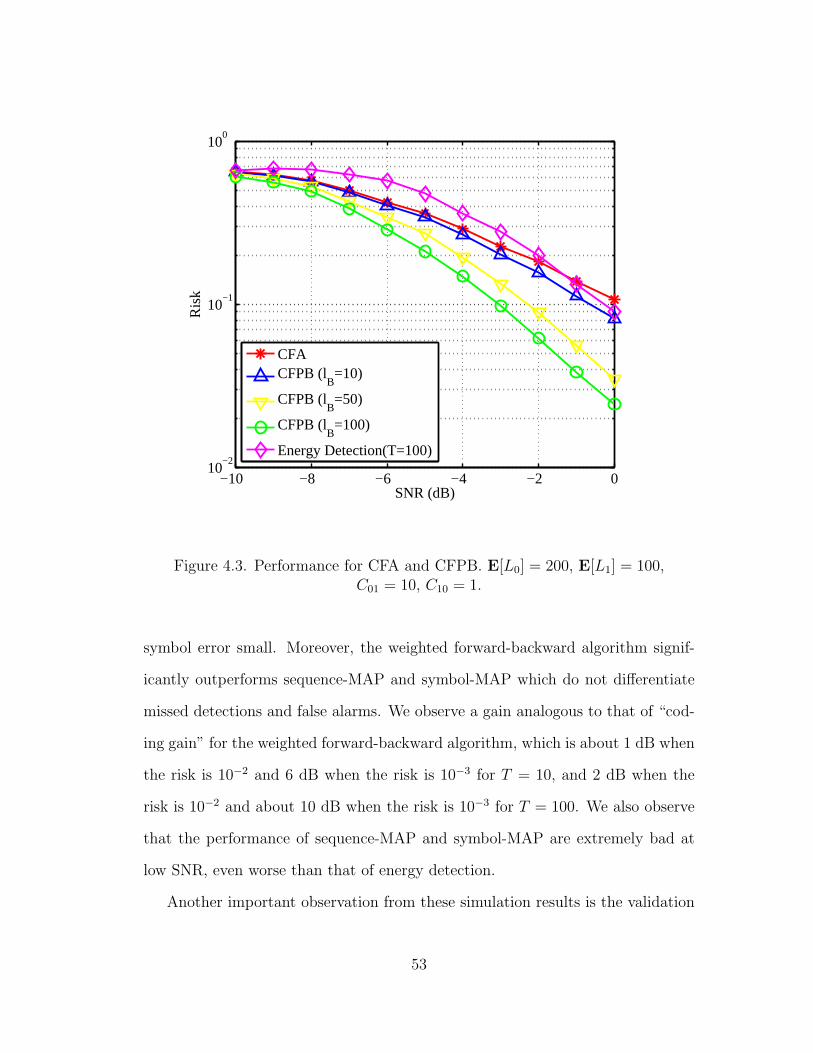
−10 −8 −6 −4 −2 010
−2
10−1
100
SNR (dB)
Ris
k
CFACFPB (l
B=10)
CFPB (lB=50)
CFPB (lB=100)
Energy Detection(T=100)
Figure 4.3. Performance for CFA and CFPB. E[L0] = 200, E[L1] = 100,C01 = 10, C10 = 1.
symbol error small. Moreover, the weighted forward-backward algorithm signif-
icantly outperforms sequence-MAP and symbol-MAP which do not differentiate
missed detections and false alarms. We observe a gain analogous to that of “cod-
ing gain” for the weighted forward-backward algorithm, which is about 1 dB when
the risk is 10−2 and 6 dB when the risk is 10−3 for T = 10, and 2 dB when the
risk is 10−2 and about 10 dB when the risk is 10−3 for T = 100. We also observe
that the performance of sequence-MAP and symbol-MAP are extremely bad at
low SNR, even worse than that of energy detection.
Another important observation from these simulation results is the validation
53

−10 −5 0 5 10 15 20 25 3010
−3
10−2
10−1
100
SNR (dB)
Ris
k
CFACFPB, l
B=1
CFPB, lB=4
CFPB, lB=10
CFPB, lB=100
Figure 4.4. Performance for CFA and CFPB. E[L0] = 200, E[L1] = 100,C01 = 10, C10 = 1.
of the existence of the risk floor for energy detection. We notice that the risks
for the weighted forward-backward algorithm decrease with asymptotically fixed
slopes as SNR increases, however, for energy detection the risk approaches the
risk floor and cannot be decreased, regardless of the window length. The risk
floor shown in the simulation results also validates the theoretical analysis in
(3.46). For T = 10, RF = 0.003 by Equation (3.46), and the simulation result
in Figure 4.5 gives RF = 0.003 as well. For T = 100, RF = 0.032 by Equation
54

(3.46), which is very close to RF = 0.031 given by simulation results in Figure 4.6.
Therefore, (3.46) appears to be a good theoretical approximation for computing
the risk floor of energy detection.
0 5 10 15 20 25 30 35 4010
−4
10−3
10−2
10−1
100
101
SNR (dB)
Ris
k
Energy DetectionSequence−MAPSymbol−MAPWeighted Forward−Backward
Figure 4.5. The risk floor for energy detection. E[L0] = 2000,E[L1] = 1000, T = 10, C01 = 10, C10 = 1.
55

−10 −5 0 5 10 15 2010
−4
10−3
10−2
10−1
100
101
SNR
Ris
k
Energy DetectionSequence−MAPSymbol−MAPWeighted Forward−Backward
Figure 4.6. The risk floor for energy detection. E[L0] = 2000,E[L1] = 1000, T = 100, C01 = 10, C10 = 1.
56

CHAPTER 5
IMPLEMENTATION OF ENERGY DETECTION AND SEQUENCE
DETECTION ALGORITHMS
This chapter describes the implementation of a simple spectrum sensing system
on a SDR platform. We first develop a self-adaptive algorithm for the secondary
user to learn the environment. We then implement both energy detection and
complete forward sequence detection algorithm for spectrum sensing in the SU
and test their performance in the low SNR scenario. We plot the detection risk
versus SNR for both detectors. From the experimental results, an advantage of
the sequence detector over the traditional energy detector can be observed.
5.1 Experimental Setup and System Parameters
The goal of the implementation in this chapter is to see the advantage of the
proposed sequence detection algorithm over the traditional energy detection in
the form of detection risk. As we focus on the performance of spectrum sensing
schemes in the SU, our cognitive radio system is comprised of two nodes for
simplicity: a primary transmitter and a secondary user that is monitoring the
spectrum constantly. Both the PU and the SU are equipped with antenna in a
wireless environment. Moreover, these two nodes are fixed without any mobility.
In the implementation, the primary transmitter takes a packet-based slotted
structure. It accesses the channel in a bursty manner, with the time duration
57

of an ON and OFF periods both follow a geometric distribution, which makes
the PU’s channel access pattern a Markov chain. This is artificially generated
by our own C++ signal processing block. The secondary user is assumed to be
aware of the slotted structure and the distribution of an ON/OFF period, but not
synchronized with the PU. In fact, synchronization is very difficult for low SNR,
especially when the timing and frequency offsets come into play in the real world.
To implement an energy detector, the secondary user needs to know the power
of the noise and the received primary signal. To implement sequence detector, the
secondary user should have perfect knowledge of the probability density function
of the primary signal under each state. In our demonstration, all these parameters
are estimated by the SU using a correlation-based, self-adaptive algorithm. This,
however, will require the PU to transmit in certain fixed and known pattern at
the beginning of its transmission.
In the implementation, cumulative moving average is used to estimate the noise
and signal power level as well as their variances. Cumulative moving average is
also called long running average. It is an iterative way to get the average of all
of the streaming data up until the current data point. Let mt be the cumulative
moving average at time instant t. mt is updated by
mt+1 =at+1 + t ·mt
t+ 1, (5.1)
where at is the current data in the streaming data sequence and m0 can be ini-
tialized to 0. The estimated parameters are then used in generating threshold for
the energy detector and the revised sequence detector. There are several reasons
why cumulative moving average is used. First, it minimizes the memory size since
only the most recent data needs to be stored. Second, compared to storing all of
58

the data and calculating the sum and dividing by the number of data points, the
cumulative moving average method averages the computation into each sensing
period and avoid the massive computation in one period, which, with high proba-
bility (almost for sure in practice), will incur the USRP overrun (will be discussed
in more details in Section 5.6.1.2).
In order to estimate the missed detection probability and the false alarm prob-
ability, we need to record the activity of the PU and the sensing result of the SU
and synchronize their starting point. We then use separate Matlab functions
to estimate these probabilities. Note that we use the term “estimate” instead of
“compute” because, for one thing, the perfect synchronization point is hard to find,
and for another, sampling rate offset discussed in more detail in Section 5.6.1.3)
between the PU and the SU exist, which will make the records of the PU and the
SU shifted by some unknown factor from time to time.
5.2 Primary Transmission
The transmission parameters and the artificially generated ON-OFF Markov
state structure of the PU is discussed in this section.
5.2.1 Transmission Parameters
The implementation is built in the 2.4 GHz ISM frequency band. The primary
transmitter transmits GMSK symbols at a bit rate of 100 kbits/s. Root-Raised
Cosine (RRC) pulses are used with a roll-off factor α = 0.35. Therefore, the
nominal baseband bandwidth B is
B =1 + α
2R = 67.5 KHz. (5.2)
59

The format for each packet is shown in Figure 5.1. Note that though no
primary reception is considered, we still use the standard packet format defined in
GNU Radio. The preamble contains the training sequence for channel estimation.
An access code is used to identify the beginning of the payload. The header
contains payload length information. CRC is Cyclic Redundancy Check and the
last padding byte is added by USRP. Payload is the user-defined data and its
length must be between 0 and 4,096 bytes. The number of samples in each packet
is calculate in the following way:
ns packet tx = (s payload+ s redundancy) · sample per symbolbit per symbol
· 8Bits
Bytes(5.3)
Preamble Access Code Header Payload CRC Pad2 Bytes 4 Bytes 4 Bytes8 Bytes 1 Bytes0 ! 4096Bytes
Figure 5.1. Packet format.
Other parameters related to the primary transmission are defined in Table 5.1.
5.2.2 Primary User’s Channel Access Structure
The PU accesses the channel by an artificially designed Markov chain model.
As mentioned above, the primary transmission is packet-based. One packet trans-
60

mission is the smallest possible time period that the primary transmitter can
occupy the channel. Each busy period (ON state) must be multiple of a packet.
For simplicity, we assume an idle period (OFF state) to be multiple of a packet as
well. At the beginning of the transmission, the PU periodically transmits fixed-
length pilot signals with ns pilot tx samples, with quiet periods of equal length in
between, as shown in Figure 5.2. We call a complete transmission of an ON pilot
sequence followed by an OFF pilot sequence one period of pilot sequence.
An ON pilot sequence An OFF pilot sequence
One period of ON-OFF pilot sequence
Mixed state Mixed stateAll ON state All OFF state
Sensing window Sensing window Sensing window Sensing window
Figure 5.2. Pilot structure and half-pilot-size sensing window.
In fact, the PU is not actually silent in an OFF period. Instead, it simply
sends all zeros to the USRP to transmit. This “fake” OFF signal generation in
the demonstration is a result of certain limitations both from the software and from
the USRP. From the software point of view, although the sleep function in python
can be used to generate the OFF period, it is not precise and therefore hard to be
fit into a Markov model whose transition probabilities are known precisely. From
61

the hardware point of view, the time for the USRP to switch from “transmitting”
to “silent” (and vice versa) is significant and may be much longer than the time
to transmit a packet.
After the pilots transmission, the PU begins to access the channel in a Markov
chain modeled way, as shown in Figure 5.3. Specifically, the number of packets
in an ON state and an OFF state follow geometric distributions with parameters
p10 and p01, respectively. The entire transmission structure of the PU is shown in
Figure 5.3.
One period of ON-OFF pilot sequence
· · · · · · · · · · · ·
n pilot repeat pilot periods Markov chain modeled transmission
Figure 5.3. PU’s channel access structure.
5.3 Spectrum Analysis, Modeling and Learning by Secondary User
To implement any detector, the SU needs to know at least the received SNR.
We can certainly estimate this parameter offline and feed them into the software
engine of the SU. However, this is not preferable in practice because, for one thing,
both the noise power and the received signal power are subject to change and the
offline estimation may become outdated very soon, and for another, we want the
62

detectors to be as intelligent as possible. In our framework, the SU will estimate
TABLE 5.1
Implementation parameters for wireless system
Variable name Value Definition
s payload 1980 size of payload (in bytes)
s redundancy 20 size of preamble, access code, header, CRC andUSRP pad in total (in bytes)
ns pilot tx 160000 number of samples in an ON/OFF pilot sequencein the transmitter
ns pilot rx 160000 number of samples in an ON/OFF pilot sequencein the receiver
ns packet tx 32000 number of samples in a packet in the transmitter
ns packet rx 32000 number of samples in a packet in the receiver
ns win 32000 number of samples in a sensing window
n packet in pilot 5 number of packets in each ON/OFF pilot period
n pilot repeat 5 how many times the ON-OFF pilot sequence re-peats before the Markov transmission
n E ON 10 Expected number of packets in an ON state
n E OFF 10 Expected number of packets in an OFF state
interp 128 FPGA interpolation factor on the transmitter
decim 64 FPGA decimation factor on the receiver
bit per symbol 1 bit per symbol
sample per symbol 2 sample per symbol
63

the received SNR based on the PU’s pilot signals. In order to do so, it should
first detect the starting point of the pilot transmission. The software engine of
the SU also needs to be robust enough to differentiate any bursty variation in
noise (background) from the real pilot transmission to avoid a false declaration.
Therefore, the software engine of the SU is implemented in three states (modes):
• PROBING.
• TRACKING.
• SENSING.
A flow graph showing how the software engine of the SU works in our experi-
mental framework is illustrated in Figure 5.4. We will discuss the functionalities
of each state in detail in the following parts of this section.
64

InP
RO
BIN
Gst
ate:
stor
eda
ta,
InT
RA
CK
ING
stat
e:st
ore
data
,co
mpu
teco
rrel
atio
n,co
unt
mat
ched
patt
erns
InSE
NSI
NG
stat
e:se
ndda
tato
sens
ing
engi
neco
mpu
teco
rrel
atio
n
Cor
rela
tion
exce
eds
cert
ain
thre
shol
d?ti
me,
num
ber
ofm
atch
ed
thre
shol
d?
Aft
ertr
acki
ngen
ough
patt
erns
exce
eds
Pre
pare
for
trac
king
:se
tst
ate
toT
RA
CK
ING
,se
tst
ate
toSE
NSI
NG
,se
tst
ate
toP
RO
BIN
G,
begi
nes
tim
atin
gsi
gnal
pow
eran
dsy
nchr
oniz
ing
poin
t
Upd
ate
nois
epo
wer
and
corr
elat
ion
thre
shol
d
Pre
pare
for
prob
ing:
Pre
pare
for
sens
ing:
chan
gew
indo
wle
ngth
,se
tsi
gnal
and
nois
epo
wer
and
thre
shol
dcl
ear
trac
king
hist
ory,
upda
tetr
acki
ngth
resh
old
SUst
ate
Yes
Yes
No
No
Inco
min
gse
nsin
gda
ta
Sens
ing
resu
lt
PR
OB
ING
TR
AC
KIN
GSE
NSI
NG
Fig
ure
5.4.
Flo
wgr
aph
ofth
ese
lf-a
dap
tive
cogn
itiv
esp
ectr
um
sensi
ng
engi
ne.
65

5.3.1 SU in PROBING State
The primary goal of the PROBING mode is to find the starting point of the
primary transmission. Along the way, the SU has to estimate the power level when
the PU is not transmitting. Therefore, the SU has three tasks to accomplish in
the PROBING mode:
• Estimate the noise power. This is done by using half-pilot-size power esti-
mator and cumulative moving average algorithm.
• Continuously update the correlation threshold based on the noise power
and variation. This threshold is to be used by the correlator to declare the
starting point of the primary transmission.
• Pass recent data to the correlator. If the correlation exceeds certain thresh-
old, declare the start of the primary transmission and leave PROBING mode
to TRACKING mode. Otherwise, continue probing.
The power estimator is actually implemented as an energy detector (only
collects samples and generates test statistics without comparing to any thresh-
old) with a half-pilot-size sensing window. Half-pilot-size means that the window
length of the power estimator is half of the size of an ON (or OFF) pilot sequence
(in samples). Note that all the energy detectors in this thesis are implemented by
type (a) as shown in Figure 2.2.2. Though the SU is not synchronized with the
PU, a half-pilot-size sensing window will not mix up samples from different states
for every other sensing window. In fact, if the PU is transmitting pilot signals, the
samples collected by the four consecutive windows must be from: mixed-state, all-
ON-state, mixed-state, all-OFF-state, with the order of appearance fixed in this
way. This is illustrated in Figure 5.2. The only exception occurs when the SU
66

is coincidentally synchronized with the PU. In this case, the samples in the four
consecutive windows should be from: all-ON-state, all-ON-state, all-OFF-state,
all-OFF-state. It still fits the pattern of alternating between all-ON-state and
all-OFF-state for every other window. Therefore, we only make discussion based
on the general case in which mixed-state windows exists with the realization that
the results apply to the special case as well.
Let Yt be the SU’s received sample at time t. Let Zn be the n-th output of the
half-pilot-size power estimator. Zn can be computed by
Zn =1
L
nL∑t=(n−1)L+1
|Yt|2, (5.4)
where L = ns pilot rx/2 is the number of samples of a half-pilot-size sensing
window. Since the ADC rate at the receiver is 64M samples per second, the
DAC rate at the transmitter is 128M samples per second, the decimation rate at
the receiver is decim, and the interpolation rate at the transmitter is interp, the
relationship between ns pilot tx and ns pilot rx is
ns pilot rx64Mdecim
=ns pilot tx
128Minterp
, (5.5)
which leads to
ns pilot rx =ns pilot tx
2· interpdecim
. (5.6)
Let µz,n and σ2z,n be the estimation of the mean and the variance of Zn, re-
spectively. Note that µz,n is also the estimation of the noise power σ2w if there
is no primary transmission. By cumulative moving average, µz,n and σ2z,n can be
67

updated iteratively by
µz,n =(n− 1)µz,n−1 + Zn
n(5.7)
σ2z,n =
(n− 1)σ2z,n−1 + (Zn − µn)2
n(5.8)
The correlator shown in Figure 5.5 is the key element in both the PROBING
and the TRACKING modes. If the SNR is very low, it is impossible to mark the
starting point of the primary transmission from the power level only, especially
when the signal and noise power levels are not known a priori.
All ON Mixed All OFFMixed All OFF MixedMixed All OFFAll ON
Correlator
Incoming sensing data sequence
!1 +1
· · · · · ·
0 0
+
A sensing window
Figure 5.5. Correlator for half-pilot-size power estimator.
In the following we briefly discuss how the correlator works in finding the
starting point as well as tracking the PU in pilot transmission. Let Rn be the
68

output of the correlator at the n-th window. Obviously,
Rn = Zn − Zn−2. (5.9)
Therefore, if there is no primary transmission,
E[R] = 0, (5.10)
Var[R] = 2σ2z . (5.11)
After the PU starts to transmit the pilot signal, suppose Zk is the output of the
first all-ON-state window. In this case, Zk−2 must be the output of an all-OFF-
state window as discussed before. For consistency, let σ2x be the power of the
received signal from the PU. Therefore,
E[Rk] = E[Zk]− E[Zk−2] = (σ2x + σ2
w)− σ2w = σ2
x (5.12)
Hence, if Rn exceeds a certain level, the SU can declare the start of the pilot
transmission. Let µr,n and σ2r,n be the estimation of mean and variance of R at
the n-th window, respectively. µr,n and σ2r,n can be computed in the same way as
in Equations (5.7, 5.8). In our demonstration, the declaration rule is set to be
Rn > ασr,n−2. (5.13)
where α is a tunable, which is set to be 10 initially and will increase by one every
time a false declaration is made.
The reason to use σr,n−2 instead of σr,n or σr,n−1 in Equation (5.13) is obvious
since with high probability a mixed-state window will be included in computing
69

σr,n and σr,n−1, which makes the estimation inaccurate.
5.3.2 SU in TRACKING State
Since the noise may be subject to certain variations and other unintended
signals may occasionally appear, the PROBING mode is likely to give a false
declaration from time to time. The leading goal of the TRACKING mode is
to confirm the primary transmission. The TRACKING mode always follows the
PROBING mode after the SU declares the start of the primary transmission. The
TRACKING mode has three tasks to accomplish:
• Further decide whether the declaration from the PROBING mode is reliable
or not (the PU actually starts transmission or not).
• Estimate the received signal power from the PU, and, along with the esti-
mated noise power, set threshold for energy detector.
• Roughly synchronize the SU with the PU.
It is worth noting that we are talking about a very week synchronization here
because by synchronization, we can estimate the probabilities of false alarm and
missed detection from the PU’s activity report and the SU’s sensing report. This
is done by separate Matlab function afterwards.
Further confirmation of the PU’s transmission is done by analyzing the fol-
lowing 4(n pilot repeat− 2) outputs of the correlator after the PROBING mode
declares the start of the PU’s transmission. If the output matches either of the two
patterns shown in Figure 5.6, the PU’s transmission is finally confirmed. Similar to
the PROBING mode, we use the outputs from the correlator to find the matched
pattern instead of using the raw test statistics. For low SNR, due to noise variation
70

and other uncertainties, neither pattern is always perfectly matched. Therefore,
we assign a matched factor β to form the threshold for pattern tracking. In our
software code, β is set to be 80%. This is to say, as long as 80% of the data
in these 4(n pilot repeat − 2) outputs matches a particular pattern, the primary
transmission is confirmed.
All OFF SamplesMixed Samples Mixed Samples All On Samples All OFF SamplesMixed Samples
All On Samples All OFF SamplesMixed Samples Mixed Samples All On Samples All OFF SamplesMixed Samples
Incoming sensing data sequence
DeclaringPU start
Trackingfrom here
DeclaringPU start
Trackingfrom here
All OFF SamplesAll OFF Samples
All OFF Samples
Pattern I: Declaring from a mixed-state-sample window
Pattern II: Declaring from an all-ON-state-sample window
Figure 5.6. Two matched patterns in the TRACKING mode
Similar to estimation of the noise power, the power level of the ON state is
estimated by the cumulative moving average of the outputs of all the all-ON-state
windows. The synchronization point is estimated by the two types of mixed-state
windows since along with the estimated power levels of ON state and OFF state,
they provide a rough estimation of how many samples are mixed from each state.
71
The SU then skips a suitable number of samples (part of the SU’s last pilot period)
and start real spectrum sensing (SENSING mode) afterwards.
It can be deduced from the above discussion that the first period of pilot
sequence serves to mark the starting point of the primary transmission, the fol-
lowing n pilot repeat − 2 periods of pilot sequence are utilized to finally confirm
the presence of the PU as well as to estimate the signal power and synchronization
point, and the last period of pilot sequence is simply ignored so that the SU can
synchronize with the PU.
The combination of the half-pilot-size power estimator (energy detector) and
the correlator provides a robust way of finding the starting point of the primary
transmission as well as estimating the received SNR. It works reasonably well even
for SNR as low as -20 dB when the related parameters are set as in Table 5.1.
5.3.3 SU in SENSING State
After tracking the PU’s pilot signal, the SU enters SENSING mode. In this
mode, the SU will be able to choose from different sensing schemes with different
parameters (such as window length). Two different detectors will be discussed in
the following section. The sensing result is then recorded in a text file to enable
the estimation of Pm and Pf , and thereafter, the detection risk.
5.4 Implementation of Energy Detection
We implement several energy detectors in this section that differ in window
length. For simplicity, the window length is assigned to be either divisor or multi-
ple of a packet size. The performance of these detectors are compared by plotting
the detection risk. To enable fair comparison, all the detectors are invoked to
72

work for the same transmission.
The result shown in Figure 5.7 is for a scenario in which the SNR is around -10
dB. Other parameters are defined as in Table 5.1. The cost factors are assigned
as C01 = 10 and C10 = 1, i.e., missed detections are 10 times more costly than
false alarms. The average channel ON time and OFF time are both 10 packets
length. The threshold of the energy detectors are set assuming that the test
statistics follows a Gaussian distribution with mean and variance generated from
the estimates in the TRACKING mode. The experimental result clearly shows
that if the window length exceeds a certain level, the performance of the energy
detector degrades. This result confirms the window length limitation for energy
detection discussed in Chapter 3.
Note again that the probabilities of missed detections and false alarms in com-
puting the risk are just rough estimation since the SU and the PU are not fully
synchronized. However, in giving a sense how varying window length will affect
the sensing performance, this estimation is enough. If further steps are taken, e.g.,
the SU makes real cognitive transmission if the channel is sensed to be free, the
probability of missed detection can be estimated from the bit error rate (BER)
of the PU and the SU. The probability of false alarm, however, is still hard to
estimate.
5.5 Implementation of Sequence Detection
Because of the variability of the real wireless systems, we change the implemen-
tation setup to a calibrated wired system as shown in Figure 5.8. This is because
the received signal in a wireless environment is not Gaussian due to fading and
time variation. Its distribution, which is critical to implement the sequence de-
73

0 5 10 15 200.35
0.4
0.45
0.5
0.55
0.6
0.65
0.7
Window length (in packets)
Ris
k
Figure 5.7. Risk level for energy detectors with different sensing windowlength.
74

Figure 5.8. System setup.
tection algorithms, are very hard or even impossible to estimate. To see this,
Figure 5.9 and Figure 5.10 illustrate the power level of an OFF and an ON pe-
riod, respectively, in a wireless environment, respectively. We can see from these
figures that neither distribution is perfectly Gaussian. In fact, they are chang-
ing in an unknown bursty manner. On the contrary, Figure 5.9 and Figure 5.10
illustrate the power level of an OFF and an ON period in a calibrated wired
environment, respectively. It can be seen from these figures that they are approx-
imately Gaussian and their distributions can be estimated in the TRACKING
mode as discussed above. We use attenuators to reduce the received signal power
in the wired environment in order not to overload the USRP receiver.
75

0 500 1000 1500 2000 2500 3000400
450
500
550
Sensing windows
pow
er le
vel
400 420 440 460 480 500 520 5400
50
100
150
200
250
300
Figure 5.9. Noise power and its histogram in a wireless environment.
76
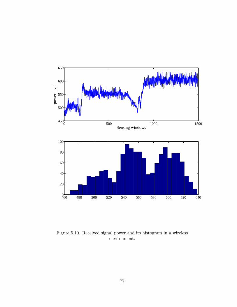
0 500 1000 1500450
500
550
600
650
Sensing windows
pow
er le
vel
460 480 500 520 540 560 580 600 620 6400
20
40
60
80
100
Figure 5.10. Received signal power and its histogram in a wirelessenvironment.
77

0 100 200 300 400 500 600 700 800 900 100011.4
11.5
11.6
11.7
11.8
11.9
12
Sensing windows
pow
er le
vel
11.4 11.5 11.6 11.7 11.8 11.9 120
20
40
60
80
Figure 5.11. Noise power and its histogram in a wired environment.
78

0 100 200 300 400 500 600 700 800 900 100022.4
22.6
22.8
23
23.2
23.4
23.6
Sensing windows
pow
er le
vel
22.4 22.6 22.8 23 23.2 23.4 23.60
20
40
60
80
100
Figure 5.12. Received signal power and its histogram in a wiredenvironment.
79

Sub-windows
Windows
Samples
Figure 5.13. Divide a sensing window into several subwindows
Due to computational limitations, we implemented a complete forward se-
quence detector as well as a complete forward partial backward sequence detector
based upon a sub-window structure, as shown in Figure 5.13. To elaborate, the
average power in each sub-window (as Zn in Section 5.3.1) is used as the input (as
Yt in Section 3.2) to the sequence detection algorithms and the sensing decision
is made per sub-window. We also use a discrete version of the proposed sequence
detection algorithms for the sake of reducing computation complexity.
Since we change our system setup from wireless to wired, we also change some
of the implementation parameters. The new parameters for implementing the
sequence detection algorithms are defined as in Table ??.
TABLE 5.2
Implementation parameters for the calibrated wired system
Variable name Value Definition
80

TABLE 5.2
Continued
Variable name Value Definition
ns pilot tx 1600 number of samples in an ON/OFF pilot sequencein the transmitter
ns subwin 1600 number of samples in a sub-window
n packet in pilot 5 number of packets in each ON/OFF pilot period
n pilot repeat 5 how many times the ON-OFF pilot sequence re-peats before the Markov transmission
n E ON 10 Expected number of packets in an ON state
n E OFF 10 Expected number of packets in an OFF state
lB 1 backward window length of CFPB
C01 10 cost factor for a miss detection
C10 1 cost factor for a false alarm
81

−10 −9 −8 −7 −6 −5 −40.95
1
1.05
1.1
1.15
1.2
1.25
SNR (dB)
Ris
k
Energy DetectionCFACFPB (l
B=1)
Figure 5.14. Estimated detection risks of energy detection, completeforward sequence detection algorithm and complete forward partial
backward sequence detection algorithm.
In Figure 5.14, the experimental performance of the CFA and CFPB detectors
are compared with a traditional energy detector that does not take memory into
account. It can be seen that by exploiting the memory in the PU’s channel access
pattern, CFA and CFPB outperform the traditional energy detection algorithm.
The experimental results also confirm the fact that CFPB does better than the
CFA. However, due to certain limitations to be discussed below, we can only
implement the CFPB with the backward length to be only one sub-window.
82

5.6 Practical Issues
The situation in the real world is never as ideal as is modeled in theory. The
hardware has certain limitations as well. Therefore, the way the implementation
framework is built and its performance is restricted and severely affected by these
non-ideal factors.
5.6.1 USRP Limitations
The hardware USRP has several limitations that shape how the software code
is implemented. We will discuss the three most relevant limitations in this sub-
section.
5.6.1.1 Switch Time
The hardware’s switch time from one state to another, for example, from
silent to sensing or from sensing to transmitting, is significant and is therefore
not negligible. If the ON state and OFF state of the PU are relatively short, the
channel state may transfer from one state to another during the USRP’s state
transition, which makes the sensing result before the USRP’s state transition
outdated.
Therefore, instead of setting the PU to the real “silent” state for an OFF
period, we simply let the USRP transmit all zeros. In this way, we generate
a bursty PU whose transmission time exhibits certain Markov property without
any FPGA configuration.
83

5.6.1.2 USRP Overrun
USRP overrun (uO) is unique for the software receiver. USRP overrun indi-
cates that the host PC is not keeping up with received data from USRP. Samples
are dropped because they are not read in time. Basically, USRP overrun occurs
if the the software code is doing too much processing per sample. In practice,
however, the software code does not need to be too complicated to incur a USRP
overrun. This imposes an limit on the computation complexity for the spectrum
sensing algorithm the SU uses in each period. One way to avoid USRP overrun
is to use greater decimation factor. Even so, the weighted sequence detection al-
gorithm with a long backward window is difficult to implement without incurring
any USRP overrun. Note that the forward probabilities can be calculated along
the way as every sample is received.
The counterpart to USRP overrun is USRP underrun (uU). USRP underrun
indicates that the PC is spending too much time processing the data and is not
sending data to the USRP fast enough. As simple as a Markov chain generator,
which just counts the number of transmitted samples in the current state until
the current length is achieved and then transitions to the other state, if not coded
carefully, will incur USRP underrun very frequently. The final software code for
Markov chain generating block at the primary transmitter is optimized in code
efficiency so as to avoid USRP underruns.
5.6.1.3 Sampling Offset
The nominal ADC rate and DAC rate are 64M and 128M samples per second,
respectively. However, sampling frequency offset exists at both ends. We call
the sampling frequency offset caused by the USRP the hardware sampling offset.
84

All ON All OFF
n periods of ON-OFF pilot sequence
4n + 1 half-pilot-size windows
Mixed Mixed All ON All OFFMixed Mixed· · · · · ·· · · · · ·PU
SU(expected)
Figure 5.15. Sampling frequency offset causes pattern mismatch andestimation errors.
Another more harmful sampling offset is caused by the software code, which we
call the software sampling offset (In fact it is not actually “sampling” offset, but
“processing” offset). If the SU does “too much” work in one period, the time to
run these codes accounts and the host PC starts to lag behind the USRP. This
will eventually cause an USRP overrun after a certain amount of time. However,
it may take much longer time to observe an USRP overrun than to transmit the
entire pilot signal, which makes the SU unaware of this sampling offset. Sampling
offset will affect the tracking process of the SU fundamentally since the expected
pattern of all-ON-state window → mixed-state window→ all-OFF-state window
→ mixed-state window in the pilot signal will be violated as shown in Figure 5.15.
Even if the mismatches are within the tolerance level, the estimation of the power
level of an ON state may be incorrect since the estimation is made by averaging
across different types of windows. Therefore, the sampling offset imposes an upper
limit on the transmission time of the PU’s pilot signal for the SU to track. The
sampling offset also has great impact on the estimation of probabilities of false
alarm and missed detection.
Though it cannot be precisely determined, the sampling frequency offset can
85
be roughly estimated from the practical observation by intentionally transmitting
the pilot signal in high SNR. Since hardware sampling offset is trivial compared
to the software sampling offset, and the software sampling offset is determined by
the amount of work the software engine done in each period, one way to reduce the
sampling offset is to minimize the average number of calculations in each period.
Note that the software sampling offset in essence is a precursor to USRP overrun,
but is more influential since it can render the estimation result wrong without
being noticed.
5.6.2 Deviation of Real World from Ideal Modeling
5.6.2.1 Imperfect Estimation
In order to implement the soft input sequence detection algorithms, the SU
needs to know the exact distribution of the primary signal and the noise. In prac-
tice, neither the noise nor the primary signal are ideally Gaussian and estimating
their distribution is fairly involved. As mentioned in the previous chapter, one
possible solution is to divide a whole sensing window into several sub-windows
and use a Gaussian approximation for the test statistics of each sub-window, as
shown in Figure 5.13. The mean and variance of the power in each sub-window
can be estimated. But note that they are imperfect estimation as well and the es-
timation error may prevent the sequence detection algorithm from outperforming
the traditional energy detection. Another solution is to quantize the observation
to make it discrete and estimate the emission probabilities from each state. How-
ever, all these solutions increase the number of calculations in each period and a
sub-window with size smaller than 100 samples will cause great software sampling
offset.
86

5.6.2.2 Bursty Interference From Unknown Sources
In practice, the false alarms and missed detections are not randomly dis-
tributed among the observations. Most of the time these two types of errors
show up in a bursty fashion. This violates the conditionally independent assump-
tion in (3.4) and makes the detection problem more involved. Moreover, false
alarms occur more often than it is supposed to be in theory. This is reasonable
since interference from other distant unknown source may appear from time to
time.
5.6.2.3 Variation in Noise and Channel Fading
From the experimental observation, the noise power of a given frequency band
is not constant, but changing slowly around a certain level. The good point is that
the “coherence time” of the noise power is much longer than the coherence time
of the fading. Therefore, its effect can be neglected. The fading of the channel,
however, cannot be neglected. We make the primary users whole transmission
smaller than the channel coherence time, therefore the estimated SNR would not
go outdated and the estimation of false alarm and missed detection probabilites
would make sense as the threshold is chosen based upon the received SNR.
87

CHAPTER 6
CONCLUSIONS AND FUTURE WORK
Dynamic spectrum access, and cognitive radio more generally, are promising
solutions to the spectral crowding problem that introduces the opportunistic usage
of frequency bands that are not efficiently utilized by licensed users. Spectrum
sensing is the key functionality to enable dynamic spectrum access. Traditional
PHY layer sensing schemes such as energy detection do not consider the primary
user’s channel access pattern. In this work, we propose several new PHY layer
spectrum sensing schemes that exploit Markov memory of the primary user’s ac-
cess pattern. These new schemes take a sequence detection structure and therefore
are called sequence detection algorithms for spectrum sensing. Our algorithms are
based on the Viterbi algorithm and the forward-backward algorithm, which are
well-known in the channel coding literature. The latter algorithms allow differ-
ent cost factors to be assigned to different types of detection errors, i.e., missed
detections and false alarms.
Two advanced sequence detection algorithms for spectrum sensing are pro-
posed in this work. The complete forward algorithm (CFA) makes the decision
only for the current time instant, based only on the forward probabilities. The
complete forward partial backward algorithm (CFPB) provides a tradeoff between
sensing performance and sensing delay and computation complexity by computing
a few backward probabilities.
88

In comparing the performance of the proposed sequence detection algorithms
with the traditional PHY layer schemes, we observe new fundamental limitations
for energy detection and coherent detection. The risk floor is a risk level that the
traditional sensing schemes cannot pass below even with arbitrarily large SNR.
The window length limitation sets an upper limit on the window length before
performance of a traditional PHY layer detector degrades. These two limitations
both result from the PU’s finite dwell time in accessing the channel. Numerical
results show the advantage of the sequence detection algorithms as well as the
limitations for traditional PHY layer detection algorithm.
Another important contribution of this work is the practical implementation
of the above-mentioned spectrum sensing schemes as well as the self-adaptive
learning by the secondary user. For many practical reasons arising from the hard-
ware and software limitations, we implement a version of the complete forward
sequence detection algorithm for a calibrated wired system and show its advantage
over energy detection through several sets of preliminary experimental results.
Many extensions can be pursued from this foundation. First, a slightly modi-
fied version of the sequence detection algorithm can be made to predict the channel
state for the next time instant/subwindow/window. We expect this sequence pre-
diction algorithm to be important in a real cognitive radio system. Second, we
can extend the sequence detection algorithm to more complicated cognitive sys-
tems in which multiple secondary users exist or multiple frequency bands are to
be sensed. Third, we can expand upon learning the environment and the primary
user’s channel access pattern using the Baum-Welch algorithm [17].
There are several possible improvements for the SDR experimentation as well.
The most direct extension is to find an applicable way to implement a real and
89

robust sequence detection algorithm given all the constraints from hardware and
software. Another direction is to expand the cognitive system and let the sec-
ondary user really transmit after detecting a spectrum hole. This corresponds to
a real dynamic spectrum access system in which primary and secondary receivers
exist.
90

BIBLIOGRAPHY
1. S. Haykin, “Cognitive radio: brain-empowered wireless communications,”IEEE J. Select. Areas Commun., vol. 23, Feb. 2005.
2. J. Mitola, “Cognitive radio for flexible mobile multimedia communications,” inProc. IEEE Int. Workshop Mobile Multimedia Communications, 1999, pp. 310.
3. Q. Zhao, Swami, A, “A Survey of Dynamic Spectrum Access: Signal Processingand Networking Perspectives,” IEEE International Conference on Acoustics,Speech and Signal Processing, 2007.
4. A. Ghasemi, E. S. Sousa,“Spectrum Sensing in Cognitive Radio Networks: Re-quirements, Challenges and Design Trade-offs,” IEEE Communications Maga-zine, April 2008.
5. D. Cabric, A. Tkachenko, and R. W. Brodersen, “Spectrum Sensing Measure-ments of Pilot, Energy and Collaborative Detection,” Proc. of IEEE MilitaryCommunications Conference, Oct. 2006.
6. A. Sahai, N. Hoven, R. Tandra, “Some Fundamental Limits on Cognitive Ra-dio,” Proc. of Allerton Conference, Monticello, Oct 2004.
7. C. Ghosh, C. Cordeiro, D. P. Agrawal, and M. B. Rao, “Markov Chain Exis-tence and Hidden Markov Models in Spectrum Sensing,” IEEE PerCom 2009,pp. 1 - 6, Mar. 2009
8. H. Kim and K. G. Shin, “Efficient Discovery of Spectrum Opportunities withMAC-Layer Sensing in Cognitive Radio Networks,” IEEE Transactions on Mo-bile Computing, Vol. 7, No. 5, pp 533-545, May 2008
9. D. Cabric, S. M. Mishra, and R. W. Brodersen, “Implementation Issues in Spec-trum Sensing for Cognitive Radios,” Proc. Asilomar Conf. Signals, Systems,and Computers, pp. 772-776, Nov. 2004.
10. Y. C. Liang, Y. Zeng, E. Peh, and A. Hoang, “Sensing-throughput tradeofffor cognitive radio networks,” IEEE Trans. Wireless Commun., Vol. 7, No. 4,pp. 1326-1337, Apr. 2008.
91

11. N. B. Chang, and M. Liu, “Optimal Channel Probing and TransmissionScheduling for Opportunistic Spectrum Access,” IEEE/ACM Transactions onNetworking, Vol. 17, No. 6, Dec 2009.
12. X. Y. Wang, A. Wong, and P. Ho, “Extended Knowledge-Based ReasoningApproach to Spectrum Sensing for Cognitive Radio,” IEEE Transactions onMobile Computing, Vol. 9, 2010.
13. S. Huang, X. Liu, and Z. Ding, “Optimal Sensing-Transmission Structure forDynamic Spectrum Access,” IEEE InfoCom 2009.
14. Q. Zhao, L. Tong, and A. Swami, “Decentralized Cognitive MAC for DynamicSpectrum Access,” Proc. IEEE Int’l Symp. Dynamic Spectrum Access Networks(DySPAN ’05), pp. 224-232, Nov. 2005.
15. S. Huang, X. Liu, and Z. Ding, “Optimal Transmission strategies for DynamicSpectrum Access in Cognitive Radio Networks,” IEEE Transactions on MobileComputing, Vol. 8, No. 12, Dec 2009
16. G. D. Forney, “The Viterbi algorithm,” Proceedings of the IEEE, Vol. 61, pp.268-278, Mar. 1973.
17. L. R. Rabiner, “A Tutorial on Hidden Markov Models and Selected Applica-tions in Speech Recognition,” Proceedings of the IEEE, Vol. 77, pp. 257 - 286,Feb. 1989.
18. H. L. Van Trees, Detection, Estimation, and Modulation Theory part I, J.Wiley & Sous Inc., 1968.
19. G. D. Brushe, R. E. Mahony, and J. B. Moore, “A Soft Output Hybrid Algo-rithm for ML/MAP Sequence Estimation,” IEEE Transactions on InformationTheory, Vol. 44, No. 7, Nov 1998.
20. I. Akyildiz, W. Lee, M. Vuran, and S. Mohanty, “Next Generation/ DynamicSpectrum Access/Cognitive Radio Wireless Networks: A Survey,” ElsevierComputer Networks, Vol. 50, 2006, pp. 2127-2159.
21. Q. Zhao, and B. M. Sadler, “A Survey of Dynamic Spectrum Access: SignalProcessing, Networking, and Regulatory Policy,” IEEE Sig. Processing, May2007.
22. P. D. Sutton, K. E. Nolan, L. E. Doyle,“Cyclostationary Signature Detectionin Multipath Rayleigh Fading Environments,” IEEE CrownCom, pp. 408 - 413,2007
92

23. W. A. Gardner, “Measurement of Spectral Correlation,” IEEE Trans. Acoust.,Speech, Signal Processing, vol. 34, Oct. 1986.
24. P. De, “New methods for sensing bandlimited signals in Cognitive Radio,”IEEE Vehicular Technology Conference, pp. 1916 - 1920, 2007.
25. Y. Zeng, Y. Liang, “Eigenvalue based Spectrum Sensing Algorithms for Cogni-tive Radio,” IEEE Transactions on Communications, Vol. 57, pp. 1784 - 1793,2009.
26. S. M. Mishra, A. Sahai, and R. W. Broderson, “Cooperative sensing amongcognitive radios,” In IEEE International Conference on Communications, Vol.4, pp. 1658-1663, 2006.
27. G. Ganesan, and Y. Li, “Cooperative spectrum sensing in cognitive radio,part I: Two user networks,” IEEE Trans. Wireless Commun., pp. 2204 - 2213,June 2007.
28. F. Digham, M. Alouini, and M. Simon, “On the energy detection of unknownsignals over fading channels,” in Proc. IEEE Int. Conf. Commun., vol. 5, Seat-tle, Washington, May 2003, pp. 35753579.
29. P. Isomaki, N. Avessta, “An Overview of Software Defined Radio Technolo-gies,” TUCS Technical Report. No 652, December 2004 IEEE CommunicationsMagazine, Apr. 2008.
30. J. Ma, Y. Li, “Soft Combination and Detection for Cooperative SpectrumSensing in Cognitive Radio Networks,” IEEE GlobeCom, pp. 3139 - 3143 Dec.2007.
31. C. Sun, W. Zhang, K. Ben Letaief, “Cooperative Spectrum Sensing for Cog-nitive Radios under Bandwidth Constraints,” IEEE Wireless Communicationsand Networking Conference, pp. 1 - 5, 2007.
32. H. Arslan, Cognitive Radio, Software Defined Radio, and Adaptive WirelessSystems, Springer 2007
33. “Gnu radio.” http://gnuradio.org/trac/wiki.
34. “Ettus USRP.” http://www.ettus.com/
35. “Basic GNU Radio.” https://radioware.nd.edu/documentation/
93

This document was prepared & typeset with pdfLATEX, and formatted withnddiss2ε classfile (v3.0[2005/07/27]) provided by Sameer Vijay.
94
Related Documents