Design and construction of a Cherenkov detector for Compton polarimetry at the ILC

Design and Construction of a Cherenkov Detector Prototype

for Compton Polarimetry at the ILC

Christoph Bartels1,2, Joachim Ebert2, Anthony Hartin1,Christian Helebrant1,2, Daniela Kafer1, and Jenny List1

1- Deutsches Elektronen Synchrotron (DESY) - Hamburg, Germany

2- Universitat Hamburg, Germany

November 5, 2009

Abstract

This paper describes the design and construction of a prototype Cherenkov detector,which was conceived with regard to high energy Compton polarimeters to be used at theInternational Linear Collider, where beam diagnostic systems of unprecedented precisionwill complement excellent detectors at the interaction region to pursue an ambitious physicsprogramme. Besides the actual design detailed simulation studies, functional tests and firsttestbeam results are discussed. Overall, a very good agreement of the first beam data withthe expectations from Monte–Carlo simulations is observed.

1 Compton Polarimetry using Cherenkov Detectors

The measurement and control of beam parameters to permille level precision will play an impor-tant role in the ambitious physics programme [1, 2] of the International Linear Collider (ILC).Not only the luminosity and the beam energy need to be measured precisely, but also the polar-isation of the electron and positron beams have to be determined with unprecedented accuracy.While for beam energy measurements the ILC’s precision goals have already been achieved atprevious colliders, the precision of polarisation measurements has to be improved by at least afactor of two compared to the (up to now most precise) polarisation measurement of the SLDpolarimeter [3].

The polarisation measurement at the ILC will combine the measurements of two dedicatedCompton polarimeters, located upstream and downstream of the e+e− interaction point, anddata from the e+e− annihilations themselves. Each of the polarimeters should reach a systematicaccuracy of δP/P = 0.25% or better. While e+e− annihilation data will finally (after severalmonths) provide an absolute scale, the polarimeters allow for fast measurements and, in caseof the upstream polarimeter, probably even resolve intra-train variations, give feedback to themachine, reduce systematic uncertainties and add redundancy to the entire system [4].

Circularly polarised laser light hits the e+(e−)-beam under a small angle and typically in theorder of 1000 electrons are scattered per bunch. The energy spectrum of the scattered particlesdepends on the product of laser and beam polarisations, so that the measured rate asymmetrywith respect to the (known) laser helicity is directly proportional to the beam polarisation. Sincethe electrons’ scattering angle in the laboratory frame is less than 10 µrad, a magnetic chicane

1

is used to transform the energy spectrum into a spatial distribution and to lead the electrons tothe Cherenkov detector of the polarimeter.A Cherenkov detector was chosen for several reasons:

(i) For relativistic electrons (β = v/c ≈ 1), Cherenkov radiation does not depend on the energyof the electrons. The light yield is obtained by integrating over the range of detectablewavelengths and over the length of traversed radiator material:

dNγ = 2πα

(

1 −1

n2β2

)

dλ

λ2d` , with:

Nγ : number of photons,` : radiator length,α : fine structure constant.

Thus, the number of Cherenkov photons (N γ) will be directly proportional to the numberof electrons per detector channel.

(ii) In order to achieve a negligible statistical error in a short time, the laser parameters arechosen such that O(1000) Compton interactions per electron bunch can be achieved. Thisresults in O(100) electrons to be detected simultaneously in a single detector channel.

(iii) Typical Cherenkov media like gases or quartz are sufficiently radiation hard to withstandthe high flux of electrons passing through the detector.

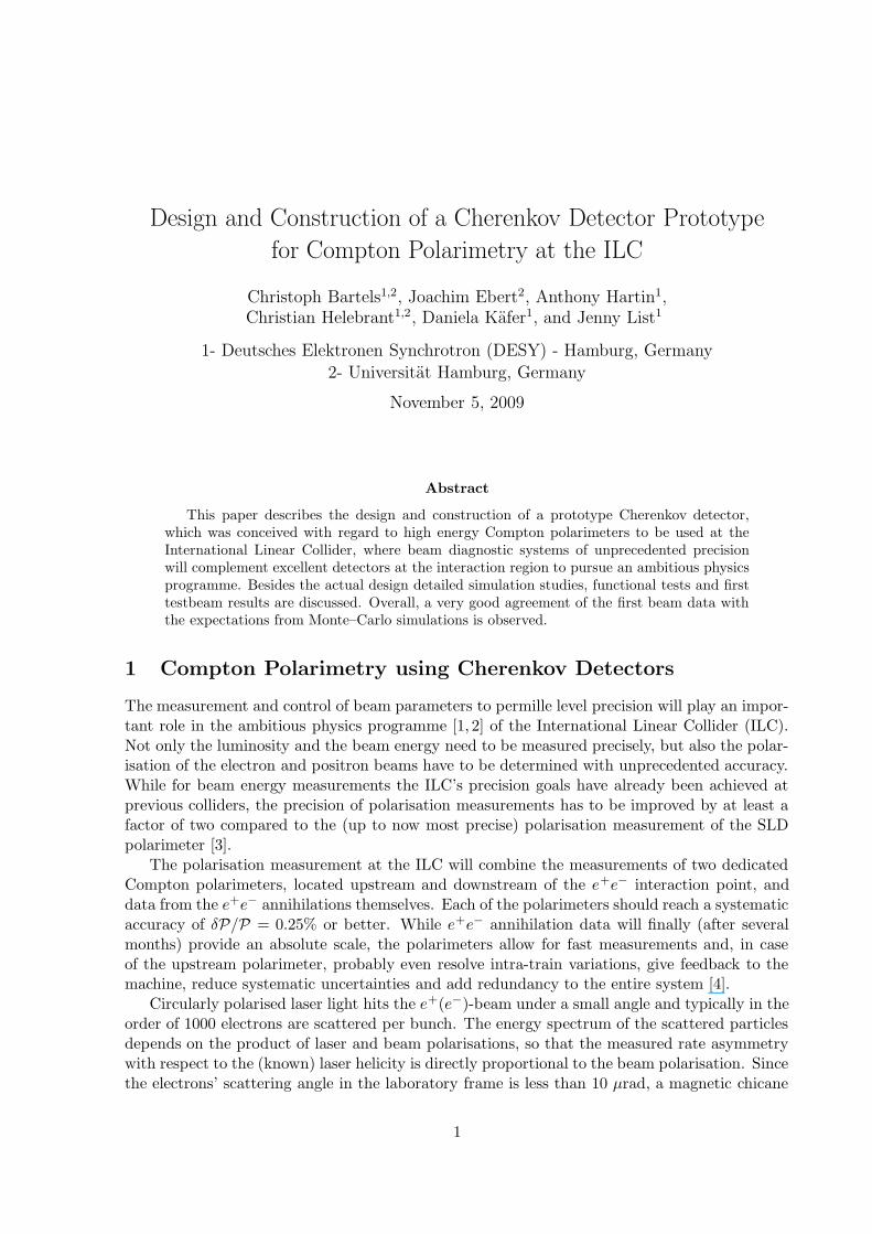
As illustrated in Figure 1(a), the detector will consist of staggered ‘U-shaped’ aluminiumtubes lining the tapered exit window of the beam pipe. The tubes are filled with a Cherenkovgas and are read out by photodetectors. Relativistic electrons traversing the basis of theseU-shaped tubes emit Cherenkov radiation which is reflected upwards in the hind U-leg to thephotodetectors, where it is measured [5]. A similar design had already been proposed in [6].

Developing a Cherenkov detector suitable for achieving the aforementioned precision ofδP/P = 0.25% demands improvements in various areas of the experimental setup. Specifically,the linearity of the detector response to the emitted Cherenkov radiation has to be addressedand a robust understanding of possible non-linearities has to be acquired in order to control andcorrect for such effects.

In the following sections, the paper briefly reviews the conceptual design, discusses in detaildesign and simulation studies of the prototype detector, and provides an overview of the con-struction and final assembly. It concludes with functional tests and first testbeam results of thefinished prototype Cherenkov detector.

2 Detector design and simulation

In this section, the conceptual design of the Cherenkov detector and the derived requirements forthe prototype are presented, along with a detailed, GEANT4-based simulation accompanyingthe design and construction phase.

To simplify further references, a right-handed coordinate system, as shown in Figure 1, willbe used throughout the rest of this document. Assuming the beam travels in positive z direction,the y-axis points upwards, and the x-axis to the left when looking in the direction of the electronbeam. References to e.g. the “left/right channel” are to be interpreted with respect to the beamdirection, i.e. the psoitive z-axis: “left” meaning the positive x-axis, “right” the negative.

2

beam

aluminum tubes

xy

z

photodetectors

LEDs

�����������������������������������������������������������������������������

�����������������������������������������������������������������������������

����������������������������������������������������

��������������������������������������������

e −beam

Cherenkovphotons

yx

z

gas−filledaluminumchannel

(a)

(b)

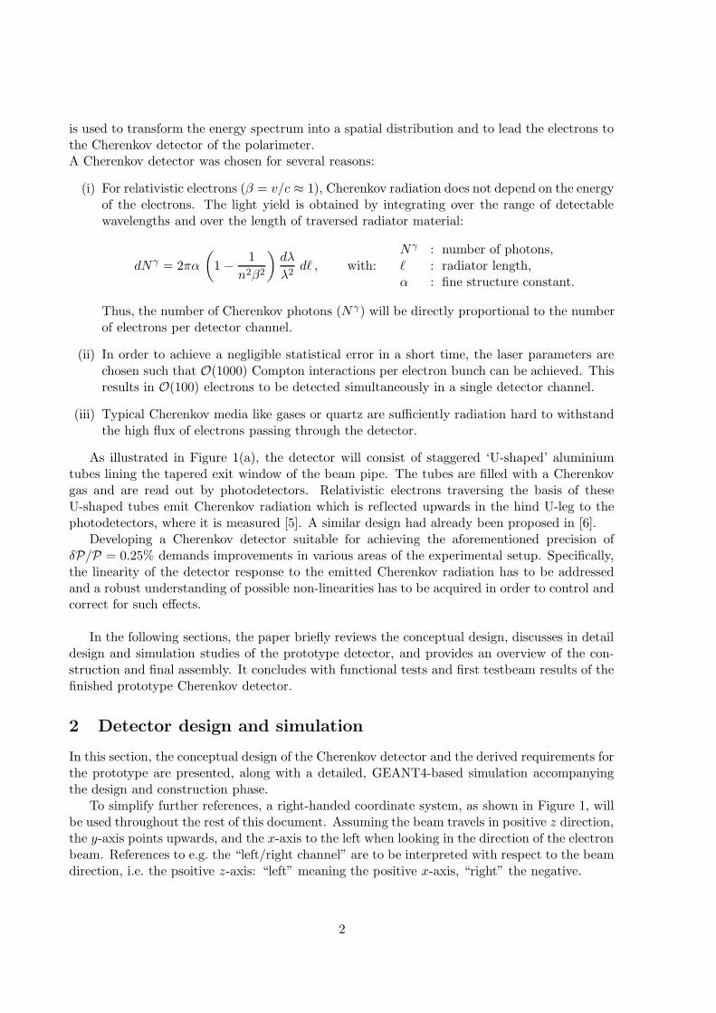
Figure 1: (a) Illustration of a Cherenkov detector as foreseen for ILC polarimetry, here, witheight readout channels; and (b) sketch of one such gas-filled aluminium channel.

2.1 Conceptual design and detector requirements

A simplified version of the envisioned detector consists of only two parallel (i.e. non-staggered)

e

PMLED (calibration)

Cherenkov photons

2

10 c

m

10 x 10 mmcross section:

15 cmA

l−tu

bes

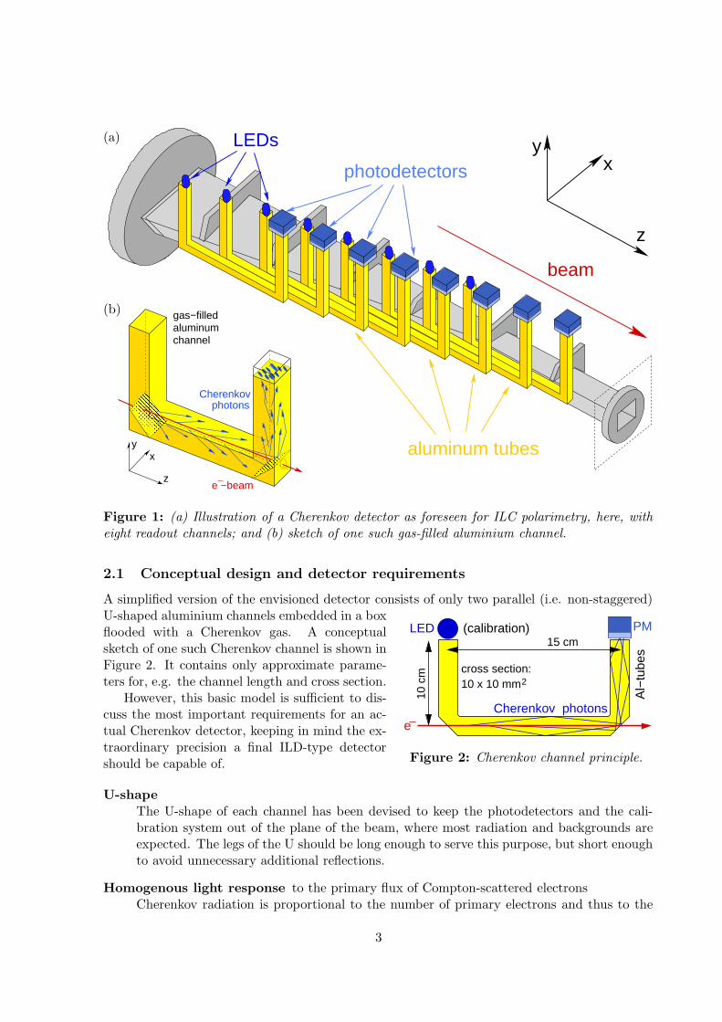
Figure 2: Cherenkov channel principle.

U-shaped aluminium channels embedded in a boxflooded with a Cherenkov gas. A conceptualsketch of one such Cherenkov channel is shown inFigure 2. It contains only approximate parame-ters for, e.g. the channel length and cross section.

However, this basic model is sufficient to dis-cuss the most important requirements for an ac-tual Cherenkov detector, keeping in mind the ex-traordinary precision a final ILD-type detectorshould be capable of.

U-shape .The U-shape of each channel has been devised to keep the photodetectors and the cali-bration system out of the plane of the beam, where most radiation and backgrounds areexpected. The legs of the U should be long enough to serve this purpose, but short enoughto avoid unnecessary additional reflections.

Homogenous light response to the primary flux of Compton-scattered electronsCherenkov radiation is proportional to the number of primary electrons and thus to the

3

length of the U-basis (see in Figure 2) where these electrons can emit Cherenkov pho-tons. Since typical Cherenkov radiation is characterised by a 1/λ2 distribution with thepeak intensity in the blue/ultraviolet range of the spectrum, high reflectivity in a widewavelength range is desirable – particularly at low wavelengths of λCher ≈ 200 − 350 nm.Manufacturing all relevant detector surfaces as smooth and planar as possible will alsohelp to generate a homogenous response.

Gas- and light-tightness .In order to control the linearity to permille level accuracy and to achieve a stable responseover macroscopic times, it is indispensable for the entire detector system to be light- andgas-tight.

Robustness with respect to backgroundsTo avoid the emittance of Cherenkov radiation from low energetic electrons, e.g. from beamgas/halo, or electrons that might have been pair produced from synchrotron radiation, agas with a high Cherenkov threshold (in the MeV-regime) should be used. A layoutallowing the photodetectors to be placed well outside the beam-plane is also mandatory.

Calibration system on the front U-legA dedicated calibration system should provide the possibility to cross-check and control thelinearity of the photodetector response independent of the presence of an electron beam.Such a system could be realized by LEDs mounted on each front U-leg or, alternatively,coupling laser light into each channel.

Thin walls between channelsSince the polarisation measurement with an ILC-type detector relies on the detection ofthe spatial distribution of Compton scattered electrons the prototype should reflect thissetup in its design. Closely spaced channels with a small cross sectional area fulfill thisrequirement. To keep the distance between the channels small the separating walls haveto be chosen as thin as possible without harming the afore mentioned specifications.

Adjustable detector position with respect to the electron beamThe position and orientation of the detector have to be adjustable with respect to theelectron beam, i.e. moveable along the x and y-axis and tiltable about all three axis inorder to arrange the centre piece of the channels parallel to the electron beam.

Contrary to the ILC-like design of staggered channels (shown in Figure 1), the prototypeCherenkov detector will consists of only two parallel, non-staggered channels. Apart from thisdifference, the smaller prototype detector should still satisfy all of the above requirements whichwill be studied in detail. However, since the two parallel channels of the prototype detector willbe placed in one solid aluminium box, it is expected that an appropriate level of gas- and light-tightness can be achieved much easier than for a multi-channel, ILC-like Cherenkov detector.This is one point where more design and engineering work will have to be invested. Therefore thechannels are constructed such that the middle wall separating the two channels of the prototypeis exchangeable, so that in the future different foils or thin sheets of aluminium could be tested.

2.2 Optical simulation using GEANT4

For the design of the prototype detector and also for the interpretation of future testbeam data,an optical simulation based on GEANT4 [7] has been created. The purpose of this simulation

4

is to determine some key figures such as the photon yield per electron, the average number ofreflections and possible asymmetry effects from the geometry and materials used. These topicswill be discussed in the next sections in detail. For a comparison of testbeam data and simula-tion see section 4.3.

All physics processes necessary to appropriately describe the emittance of Cherenkov radi-ation from relativistic electrons and any subsequent or secondary processes like multiple scat-tering, bremsstrahlung, annihilation, optical absorption, scintillation, and ionisation have beenincluded in the GEANT4 simulation. The following list provides a more detailed overview of allprocesses broken down into the different particles they are relevant for:

electrons (e−, e+): Cherenkov radiation, multiple scattering, ionisation,

bremsstrahlung, annihilation

muons (µ−, µ+): multiple scattering, ionisation,

bremsstrahlung, pair production

photons (γ): scintillation,

Optical absorption/boundary processes/Rayleigh scattering

all other particles: multiple scattering, hadron ionisation

The so-called optical processes, that appear for the photons, are only relevant for wavelengthslarger than the distance between individual atoms of the surface material, i.e. for λ � datoms.The abbreviation boundary processes stands for all processes taking place at boundary surfacesbetween different materials, including the boundaries between different dielectric media and/ordielectric-metal boundaries. All these materials have non-perfect surfaces causing reflection,refraction, and absorption of photons.

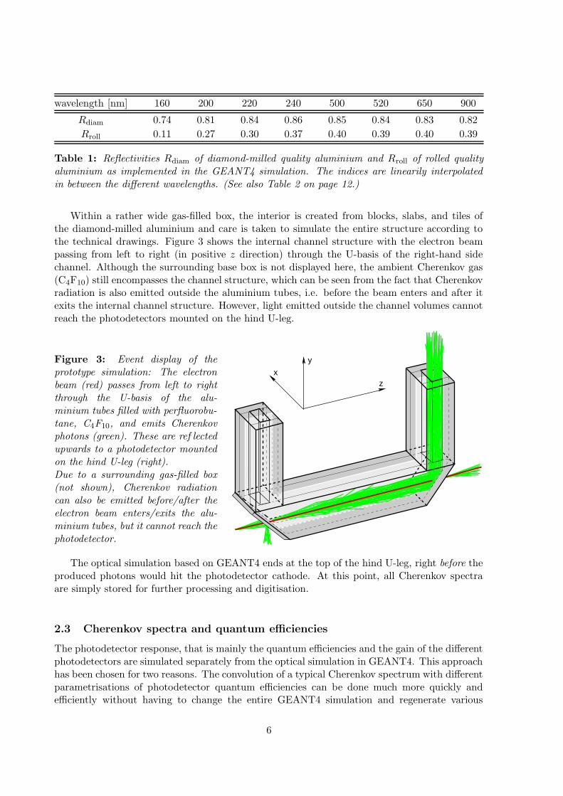
The length of the U-basis is the only relevant length for the Cherenkov process since itdetermines how long relativistic electrons can emit Cherenkov radiation while traveling throughthe gas-filled channels. To ensure the production of a sufficient number of photons per channel,this distance was chosen to be 150 mm for electrons passing through the channel centre in thetransverse plane, i.e. the (x, y)-plane (see Figure 3).

Based on earlier stand-alone studies of different types of photodetectors [8–10], it was de-cided at the beginning of the design phase which photomultipliers (PM) should be used withthe prototype, c.f. section 3.1. Due to the layout and square geometry of two multi-anodephotomultipliers (MAPMs), the channel cross section was chosen to be 8.5×8.5 mm2.

Different materials were created to simulate the inner channel structure in accordance withthe design and construction plans: aluminium for all channel walls and perfluorobutane (C4F10)with a refraction index of 1.0014, corresponding to a radiation threshold of 10 MeV, as Cherenkovgas.

The results of the reflectivity studies of different aluminium surfaces summarised in Sec. 2.6were implemented in the optical simulation software by introducing two different types of alu-minium with average refraction indices of: Rdiam ≈ 0.83 for the diamond-milled aluminiummaking up three of the four inner channel walls, and Rroll ≈ 0.37 for the two 0.15 mm-thinrolled foils of which the middle wall between both channels consists. The wavelength depen-dence of the refraction indices is implemented by a set of interpolation points as documented inTable 1 and assuming a linear behaviour of the indices in between those points.

The temperature and gas pressure inside the box are kept constant at T = 20◦ C andp = 1 atm = 1.01325 bar, respectively.

5

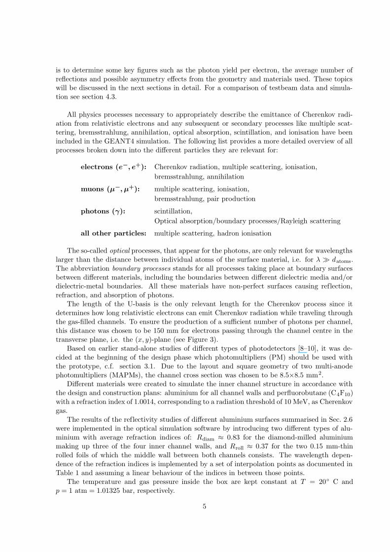
wavelength [nm] 160 200 220 240 500 520 650 900

Rdiam 0.74 0.81 0.84 0.86 0.85 0.84 0.83 0.82

Rroll 0.11 0.27 0.30 0.37 0.40 0.39 0.40 0.39

Table 1: Reflectivities Rdiam of diamond-milled quality aluminium and Rroll of rolled qualityaluminium as implemented in the GEANT4 simulation. The indices are linearily interpolatedin between the different wavelengths. (See also Table 2 on page 12.)

Within a rather wide gas-filled box, the interior is created from blocks, slabs, and tiles ofthe diamond-milled aluminium and care is taken to simulate the entire structure according tothe technical drawings. Figure 3 shows the internal channel structure with the electron beampassing from left to right (in positive z direction) through the U-basis of the right-hand sidechannel. Although the surrounding base box is not displayed here, the ambient Cherenkov gas(C4F10) still encompasses the channel structure, which can be seen from the fact that Cherenkovradiation is also emitted outside the aluminium tubes, i.e. before the beam enters and after itexits the internal channel structure. However, light emitted outside the channel volumes cannotreach the photodetectors mounted on the hind U-leg.

Figure 3: Event display of theprototype simulation: The electronbeam (red) passes from left to rightthrough the U-basis of the alu-minium tubes filled with perfluorobu-tane, C4F10, and emits Cherenkovphotons (green). These are ref lectedupwards to a photodetector mountedon the hind U-leg (right).Due to a surrounding gas-filled box(not shown), Cherenkov radiationcan also be emitted before/after theelectron beam enters/exits the alu-minium tubes, but it cannot reach thephotodetector.

x

y

z

The optical simulation based on GEANT4 ends at the top of the hind U-leg, right before theproduced photons would hit the photodetector cathode. At this point, all Cherenkov spectraare simply stored for further processing and digitisation.

2.3 Cherenkov spectra and quantum efficiencies

The photodetector response, that is mainly the quantum efficiencies and the gain of the differentphotodetectors are simulated separately from the optical simulation in GEANT4. This approachhas been chosen for two reasons. The convolution of a typical Cherenkov spectrum with differentparametrisations of photodetector quantum efficiencies can be done much more quickly andefficiently without having to change the entire GEANT4 simulation and regenerate various

6

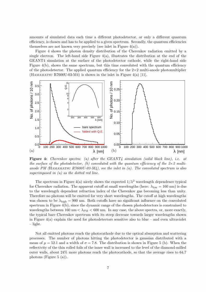
amounts of simulated data each time a different photodetector, or only a different quantumefficiency, is chosen and has to be applied to a given spectrum. Secondly, the quantum efficienciesthemselves are not known very precisely (see inlet in Figure 4(a)).

Figure 4 shows the photon density distribution of the Cherenkov radiation emitted by asingle electron. The left-hand side Figure 4(a), illustrates the distribution at the end of theGEANT4 simulation at the surface of the photodetector cathode, while the right-hand sideFigure 4(b), shows the same spectrum, but this time convoluted with the quantum efficiencyof the photodetector. The applied quantum efficiency for the 2×2 multi-anode photomultiplier(Hamamatsu R7600U-03-M4) is shown in the inlet in Figure 4(a) [11].

λ [nm]0 100 200 300 400 500 600 700 800 900 1000

No.

of p

hoto

ns /

10 n

m

0.0

0.5

1.0

1.5

2.0

2.5

3.0

3.5

bare spectrum

folded with Q.E.

λ [nm]200 300 400 500 600

Q.E

.

1

2

4

68

10

30

λ [nm]0 100 200 300 400 500 600 700 800 900 1000

No.

of p

hoto

ns /

10 n

m

0.00

0.05

0.10

0.15

0.20

0.25

(a) (b)

Figure 4: Cherenkov spectra: (a) after the GEANT4 simulation (solid black line), i.e. atthe surface of the photodetector, (b) convoluted with the quantum efficiency of the 2×2 multi-anode PM (Hamamatsu R7600U-03-M4), see the inlet in (a). The convoluted spectrum is alsosuperimposed in (a) as the dotted red line.

The spectrum in Figure 4(a) nicely shows the expected 1/λ2 wavelength dependence typicalfor Cherenkov radiation. The apparent cutoff at small wavelengths (here: λlow = 160 nm) is dueto the wavelength dependent refraction index of the Cherenkov gas becoming less than unity.Therefore no photons will be emitted for very short wavelengths. The cutoff at high wavelengthswas chosen to be λhigh = 900 nm. Both cutoffs have no significant influence on the convolutedspectrum in Figure 4(b), since the dynamic range of the chosen photodetectors is constrained towavelengths between 160 nm< λPM < 600 nm. In any case, the above spectra, or, more exactly,the typical bare Cherenkov spectrum with its steep decrease towards larger wavelengths shownin Figure 4(a) explain the need for photodetectors sensitive also to blue – and even ultraviolet– light.

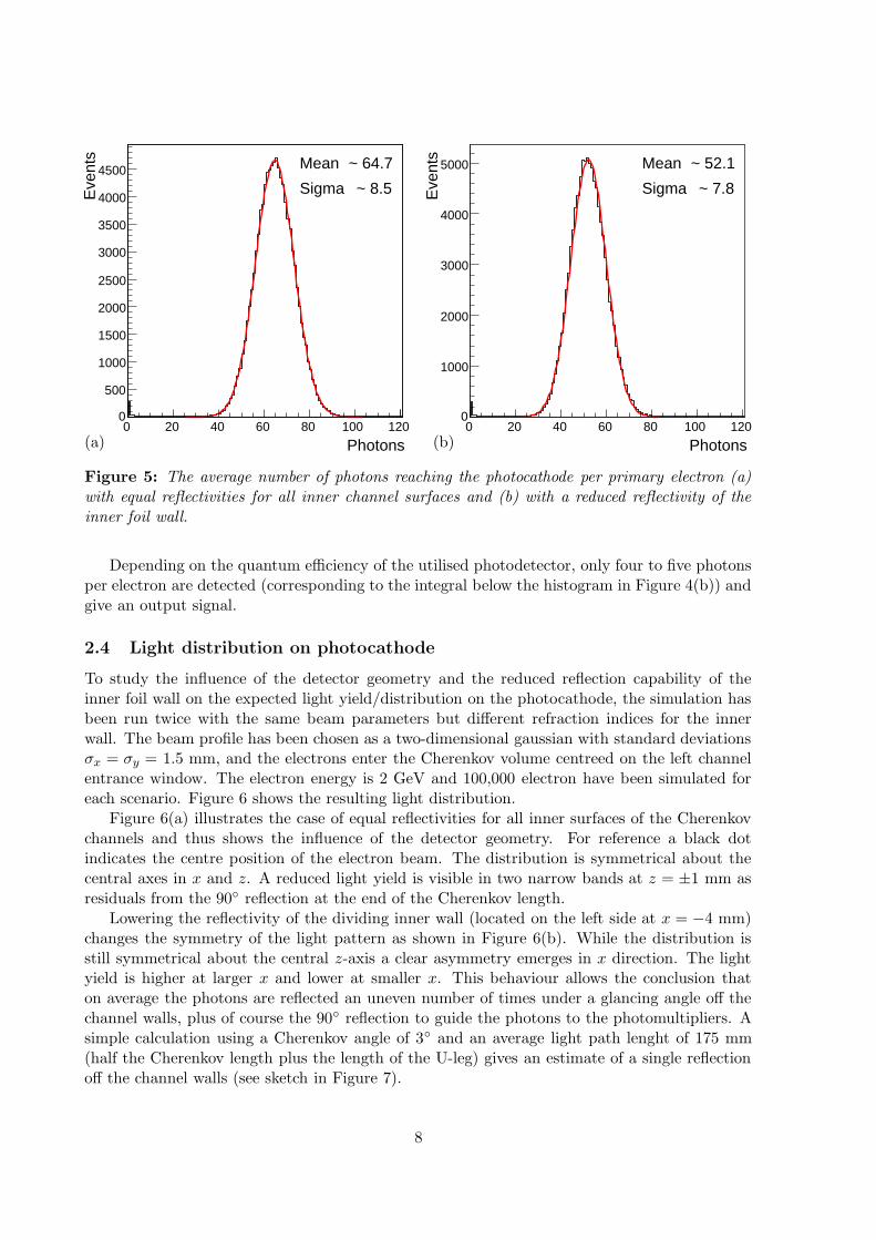
Not all emitted photons reach the photocathode due to the optical absorption and scatteringprocesses. The number of photons hitting the photodetector is gaussian distributed with amean of µ = 52.1 and a width of σ = 7.8. The distribution is shown in Figure 5 (b). When thereflectivity of the thin rolled foils of the inner wall is increased to the level of the diamond-milledouter walls, about 24% more photons reach the photocathode, so that the average rises to 64.7photons (Figure 5 (a)).

7

Photons0 20 40 60 80 100 120

Eve

nts

0

500

1000

1500

2000

2500

3000

3500

4000

4500 Mean ~ 64.7

Sigma ~ 8.5

Photons0 20 40 60 80 100 120

Eve

nts

0

1000

2000

3000

4000

5000 Mean ~ 52.1

Sigma ~ 7.8

(a) (b)

Figure 5: The average number of photons reaching the photocathode per primary electron (a)with equal reflectivities for all inner channel surfaces and (b) with a reduced reflectivity of theinner foil wall.

Depending on the quantum efficiency of the utilised photodetector, only four to five photonsper electron are detected (corresponding to the integral below the histogram in Figure 4(b)) andgive an output signal.

2.4 Light distribution on photocathode

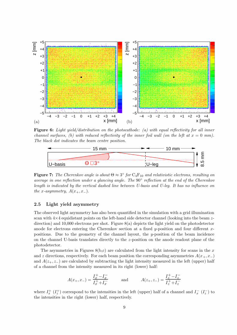
To study the influence of the detector geometry and the reduced reflection capability of theinner foil wall on the expected light yield/distribution on the photocathode, the simulation hasbeen run twice with the same beam parameters but different refraction indices for the innerwall. The beam profile has been chosen as a two-dimensional gaussian with standard deviationsσx = σy = 1.5 mm, and the electrons enter the Cherenkov volume centreed on the left channelentrance window. The electron energy is 2 GeV and 100,000 electron have been simulated foreach scenario. Figure 6 shows the resulting light distribution.

Figure 6(a) illustrates the case of equal reflectivities for all inner surfaces of the Cherenkovchannels and thus shows the influence of the detector geometry. For reference a black dotindicates the centre position of the electron beam. The distribution is symmetrical about thecentral axes in x and z. A reduced light yield is visible in two narrow bands at z = ±1 mm asresiduals from the 90◦ reflection at the end of the Cherenkov length.

Lowering the reflectivity of the dividing inner wall (located on the left side at x = −4 mm)changes the symmetry of the light pattern as shown in Figure 6(b). While the distribution isstill symmetrical about the central z-axis a clear asymmetry emerges in x direction. The lightyield is higher at larger x and lower at smaller x. This behaviour allows the conclusion thaton average the photons are reflected an uneven number of times under a glancing angle off thechannel walls, plus of course the 90◦ reflection to guide the photons to the photomultipliers. Asimple calculation using a Cherenkov angle of 3◦ and an average light path lenght of 175 mm(half the Cherenkov length plus the length of the U-leg) gives an estimate of a single reflectionoff the channel walls (see sketch in Figure 7).

8

x [mm]−4 −3 −2 −1 0 +1 +2 +3 +4

z [m

m]

−5

−4

−3

−2

−1

0

+1

+2

+3

+4

+5

0

50

100

150

200

250

x [mm]−4 −3 −2 −1 0 +1 +2 +3 +4

z [m

m]

−5

−4

−3

−2

−1

0

+1

+2

+3

+4

+5

(a) (b)

Figure 6: Light yield/distribution on the photocathode: (a) with equal reflectivity for all innerchannel surfaces, (b) with reduced reflectivity of the inner foil wall (on the left at x = 0 mm).The black dot indicates the beam centre position.

10 mm

8.5

mm

15 mm

Θ ∼ 3 oU−basis U−leg

Figure 7: The Cherenkov angle is about Θ ≈ 3◦ for C4F10 and relativistic electrons, resulting onaverage in one reflection under a glancing angle. The 90◦ reflection at the end of the Cherenkovlength is indicated by the vertical dashed line between U-basis and U-leg. It has no influence onthe x-asymmetry, A(x+, x−).

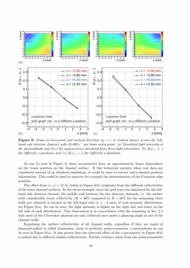
2.5 Light yield asymmetry

The observed light asymmetry has also been quantified in the simulation with a grid illuminationscan with 4×4 equidistant points on the left-hand side detector channel (looking into the beam z-direction) and 10,000 electrons per shot. Figure 8(a) depicts the light yield on the photodetectoranode for electrons entering the Cherenkov section at a fixed y-position and four different x-positions. Due to the geometry of the channel layout, the y-position of the beam incidenceon the channel U-basis translates directly to the z-position on the anode readout plane of thephotodetector.

The asymmetries in Figures 8(b,c) are calculated from the light intensity for scans in the xand z directions, respectively. For each beam position the corresponding asymmetries A(x+, x−)and A(z+, z−) are calculated by subtracting the light intensity measured in the left (upper) halfof a channel from the intensity measured in its right (lower) half:

A(x+, x−) =I+x −I

−x

I+x +I

−x

and A(z+, z−) =I+z −I

−z

I+z +I

−z

where I+x (I+

z ) correspond to the intensities in the left (upper) half of a channel and I−

x (I−z ) tothe intensities in the right (lower) half, respectively.

9

x [mm]−4 −3 −2 −1 0 1 2 3 4

A (

x ,

x

)+

−

−0.3

−0.2

−0.1

0.0

0.1

0.2

0.3 z = −2.55 mmz = −0.85 mmz = +0.85 mmz = +2.55 mm

z [mm]−4 −3 −2 −1 0 1 2 3 4

A (

z ,

z

)+

−

−0.3

−0.2

−0.1

0.0

0.1

0.2

0.3 x = −2.55 mmx = −0.85 mmx = +0.85 mmx = +2.55 mm

x [mm]−4 −3 −2 −1 0 1 2 3 4

z [m

m]

−5−4−3−2−1012345

x [mm]−4 −3 −2 −1 0 1 2 3 4

z [m

m]

−5−4−3−2−1012345

0

50

100

150

200

250

x [mm]−4 −3 −2 −1 0 1 2 3 4

z [m

m]

−5−4−3−2−1

012345

x [mm]−4 −3 −2 −1 0 1 2 3 4

z [m

m]

−5−4−3−2−1012345

(a)

(b) (c)

z-position fixed:

each graph corr. to a different z-position

x-position fixed:

each graph corr. to a different x-position

Figure 8: Scans in horizontal and vertical direction (y → z in readout plane) across the left-hand side detector channel; with 10,000 e− per beam entry point. (a) Simulated light intensity atthe photocathode and (b,c) the asymmetries calculated from these light intensities: (b) A(x+, x−)for different z-positions and (c) A(z+, z−) for different x-positions.

As can be seen in Figure 8, these asymmetries have an approximately linear dependenceon the beam position on the channel surface. If this behaviour persists when real data areconsidered instead of an idealised simulation, it could be used to extract intra-channel positioninformation. This could be used to improve for example the determination of the Compton edgeposition.

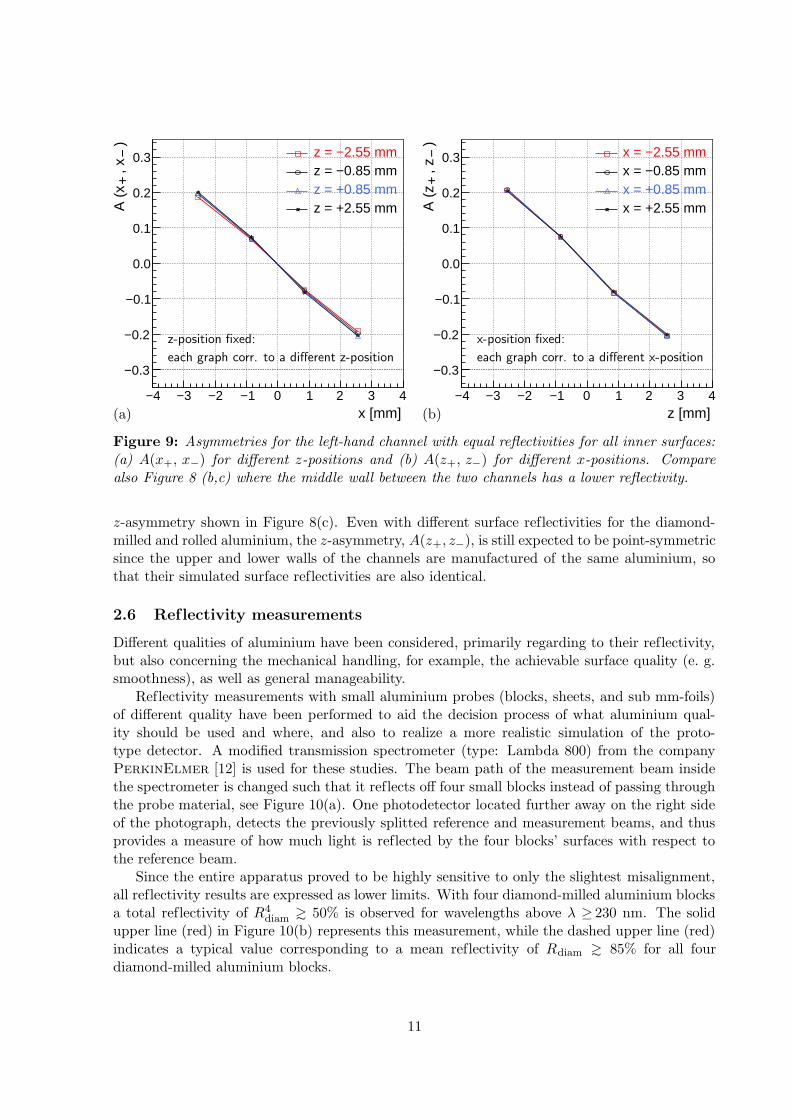
The offset from (x, z) = (0, 0) visible in Figure 8(b) originates from the different reflectivitiesof the inner channel surfaces. In the above example, since the grid scan was simulated for the left-hand side detector channel, the middle wall between the two detector channels, i.e. the surfacewith considerably worse reflectivity (R = 40% compared to R = 85% for the remaining threewalls per channel) is located at the left-hand side (x = −4 mm) of each intensity distribution,see Figure 8(a). As can be seen, the light intensity is higher on the right side and lower on theleft side of each distribution. This observation is in concordance with the reasoning in Sec. 2.4that most of the Cherenkov photons are only reflected once under a glancing angle at one of thechannel walls.

Equalising the surface reflectivities of all channel walls, regardless if they are made ofdiamond-milled or rolled aluminium, leads to perfectly point-symmetric x-asymmetries as canbe seen in Figure 9(a). It also proves that the observed offset of the x-asymmetry in Figure 8(b)is indeed due to different surface reflectivities. Further evidence arises from the point-symmetric

10

x [mm]−4 −3 −2 −1 0 1 2 3 4

A (

x ,

x

)+

−

−0.3

−0.2

−0.1

0.0

0.1

0.2

0.3 z = −2.55 mmz = −0.85 mmz = +0.85 mmz = +2.55 mm

z [mm]−4 −3 −2 −1 0 1 2 3 4

A (

z ,

z

)+

−

−0.3

−0.2

−0.1

0.0

0.1

0.2

0.3 x = −2.55 mmx = −0.85 mmx = +0.85 mmx = +2.55 mm

(a) (b)

z-position fixed:

each graph corr. to a different z-position

x-position fixed:

each graph corr. to a different x-position

Figure 9: Asymmetries for the left-hand channel with equal reflectivities for all inner surfaces:(a) A(x+, x−) for different z-positions and (b) A(z+, z−) for different x-positions. Comparealso Figure 8 (b,c) where the middle wall between the two channels has a lower reflectivity.

z-asymmetry shown in Figure 8(c). Even with different surface reflectivities for the diamond-milled and rolled aluminium, the z-asymmetry, A(z+, z−), is still expected to be point-symmetricsince the upper and lower walls of the channels are manufactured of the same aluminium, sothat their simulated surface reflectivities are also identical.

2.6 Reflectivity measurements

Different qualities of aluminium have been considered, primarily regarding to their reflectivity,but also concerning the mechanical handling, for example, the achievable surface quality (e. g.smoothness), as well as general manageability.

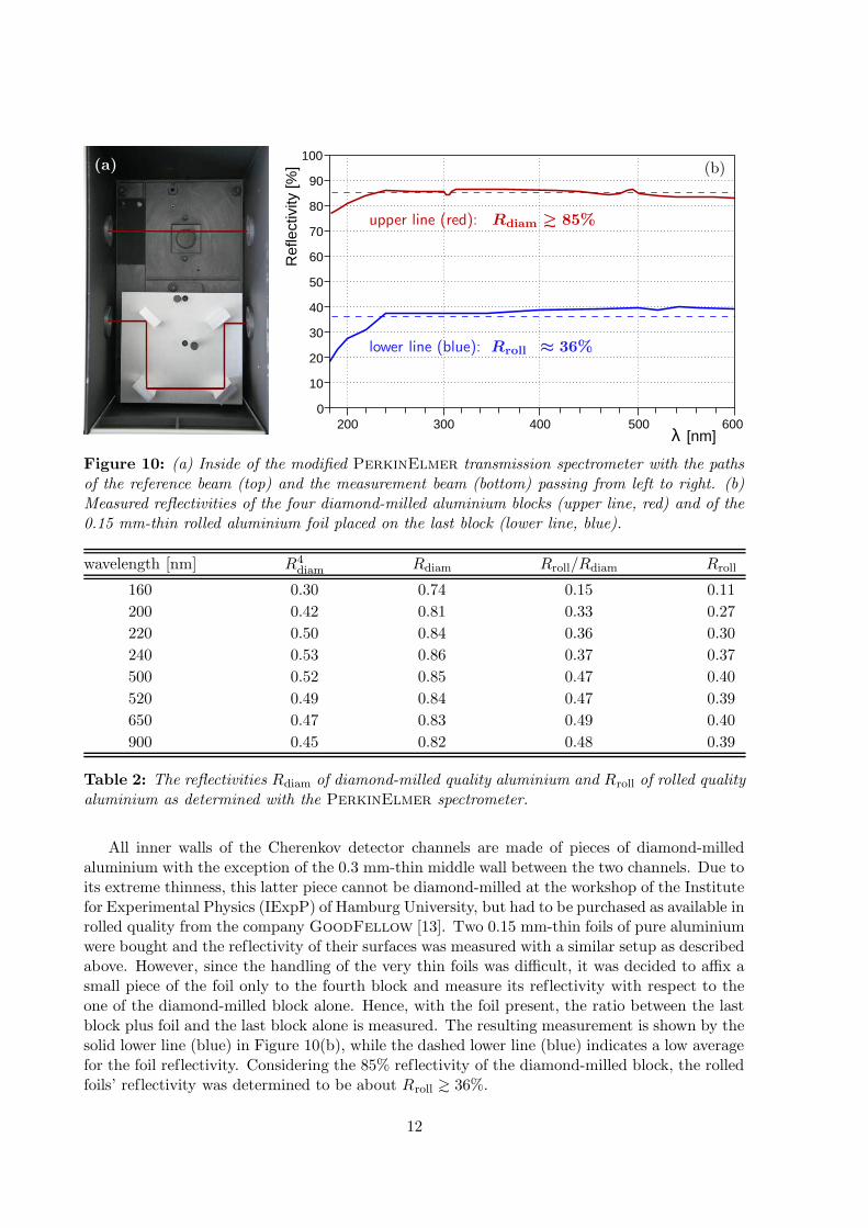
Reflectivity measurements with small aluminium probes (blocks, sheets, and sub mm-foils)of different quality have been performed to aid the decision process of what aluminium qual-ity should be used and where, and also to realize a more realistic simulation of the proto-type detector. A modified transmission spectrometer (type: Lambda 800) from the companyPerkinElmer [12] is used for these studies. The beam path of the measurement beam insidethe spectrometer is changed such that it reflects off four small blocks instead of passing throughthe probe material, see Figure 10(a). One photodetector located further away on the right sideof the photograph, detects the previously splitted reference and measurement beams, and thusprovides a measure of how much light is reflected by the four blocks’ surfaces with respect tothe reference beam.

Since the entire apparatus proved to be highly sensitive to only the slightest misalignment,all reflectivity results are expressed as lower limits. With four diamond-milled aluminium blocksa total reflectivity of R4

diam ? 50% is observed for wavelengths above λ ≥ 230 nm. The solidupper line (red) in Figure 10(b) represents this measurement, while the dashed upper line (red)indicates a typical value corresponding to a mean reflectivity of Rdiam ? 85% for all fourdiamond-milled aluminium blocks.

11

60

50

40

30

20

10

0

70

80

90

100

Ref

lect

ivity

[%]

200 300 400 500 600[nm]λ

(a) (b)

upper line (red): Rdiam ? 85%

lower line (blue): Rroll ≈ 36%

Figure 10: (a) Inside of the modified PerkinElmer transmission spectrometer with the pathsof the reference beam (top) and the measurement beam (bottom) passing from left to right. (b)Measured reflectivities of the four diamond-milled aluminium blocks (upper line, red) and of the0.15 mm-thin rolled aluminium foil placed on the last block (lower line, blue).

wavelength [nm] R4diam Rdiam Rroll/Rdiam Rroll

160 0.30 0.74 0.15 0.11

200 0.42 0.81 0.33 0.27

220 0.50 0.84 0.36 0.30

240 0.53 0.86 0.37 0.37

500 0.52 0.85 0.47 0.40

520 0.49 0.84 0.47 0.39

650 0.47 0.83 0.49 0.40

900 0.45 0.82 0.48 0.39

Table 2: The reflectivities Rdiam of diamond-milled quality aluminium and Rroll of rolled qualityaluminium as determined with the PerkinElmer spectrometer.

All inner walls of the Cherenkov detector channels are made of pieces of diamond-milledaluminium with the exception of the 0.3 mm-thin middle wall between the two channels. Due toits extreme thinness, this latter piece cannot be diamond-milled at the workshop of the Institutefor Experimental Physics (IExpP) of Hamburg University, but had to be purchased as available inrolled quality from the company GoodFellow [13]. Two 0.15 mm-thin foils of pure aluminiumwere bought and the reflectivity of their surfaces was measured with a similar setup as describedabove. However, since the handling of the very thin foils was difficult, it was decided to affix asmall piece of the foil only to the fourth block and measure its reflectivity with respect to theone of the diamond-milled block alone. Hence, with the foil present, the ratio between the lastblock plus foil and the last block alone is measured. The resulting measurement is shown by thesolid lower line (blue) in Figure 10(b), while the dashed lower line (blue) indicates a low averagefor the foil reflectivity. Considering the 85% reflectivity of the diamond-milled block, the rolledfoils’ reflectivity was determined to be about Rroll ? 36%.

12

This value should clearly be improved for the next prototype Cherenkov detector, either byhaving the thin middle wall also diamond-milled at the IExpP workshop (which may lead toa thickness of up to 0.5 mm), or by purchasing special polished or otherwise treated foil withimproved surface reflectivity.

The measured reflectivities were used in the simulation studies (Sec. 2.3). For a more realisticmodel the refractive indices were interpolated linearily between a set of different wavelengthswhich are taken from the measurement as listed in Table 2.

3 Construction of the prototype

The basic channel dimensions of the prototype, namely the length and diameter, were chosen tomatch the design criteria discussed in section 2.2. The length of the U-basis which is relevantfor the emission of Cherenkov radiation from traversing electrons, is 150 mm and the heightof the two U-legs is 100 mm. A quadratic cross section of 8.5×8.5 mm2 has been chosen tomatch the cathode geometry of four different types of photomultipliers. The best geometricalconformance between channel cross section and photocathode is intended for two square multi-anode photomultipliers, since both these PMTs offer the most possibilities in terms of positioningwith respect to the channels. See section 3.1 for further details on what types of photodetectorswill be employed, which characteristics they share, or what distinguishes them from each other.

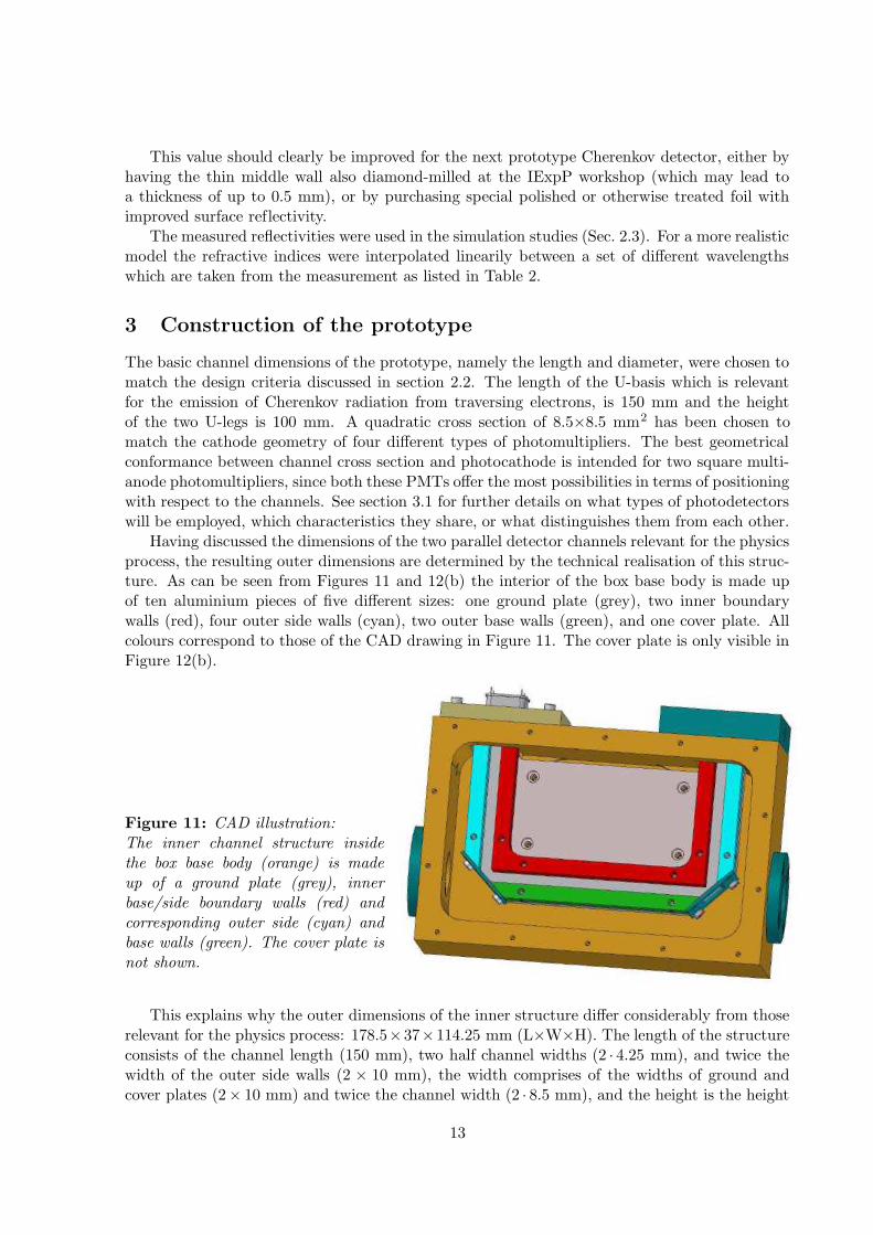
Having discussed the dimensions of the two parallel detector channels relevant for the physicsprocess, the resulting outer dimensions are determined by the technical realisation of this struc-ture. As can be seen from Figures 11 and 12(b) the interior of the box base body is made upof ten aluminium pieces of five different sizes: one ground plate (grey), two inner boundarywalls (red), four outer side walls (cyan), two outer base walls (green), and one cover plate. Allcolours correspond to those of the CAD drawing in Figure 11. The cover plate is only visible inFigure 12(b).

Figure 11: CAD illustration:The inner channel structure insidethe box base body (orange) is madeup of a ground plate (grey), innerbase/side boundary walls (red) andcorresponding outer side (cyan) andbase walls (green). The cover plate isnot shown.

This explains why the outer dimensions of the inner structure differ considerably from thoserelevant for the physics process: 178.5×37×114.25 mm (L×W×H). The length of the structureconsists of the channel length (150 mm), two half channel widths (2 · 4.25 mm), and twice thewidth of the outer side walls (2 × 10 mm), the width comprises of the widths of ground andcover plates (2× 10 mm) and twice the channel width (2 · 8.5 mm), and the height is the height

13

of an U-leg (100 mm) plus the height of the outer base wall (10 mm) and half a channel width(4.25 mm).

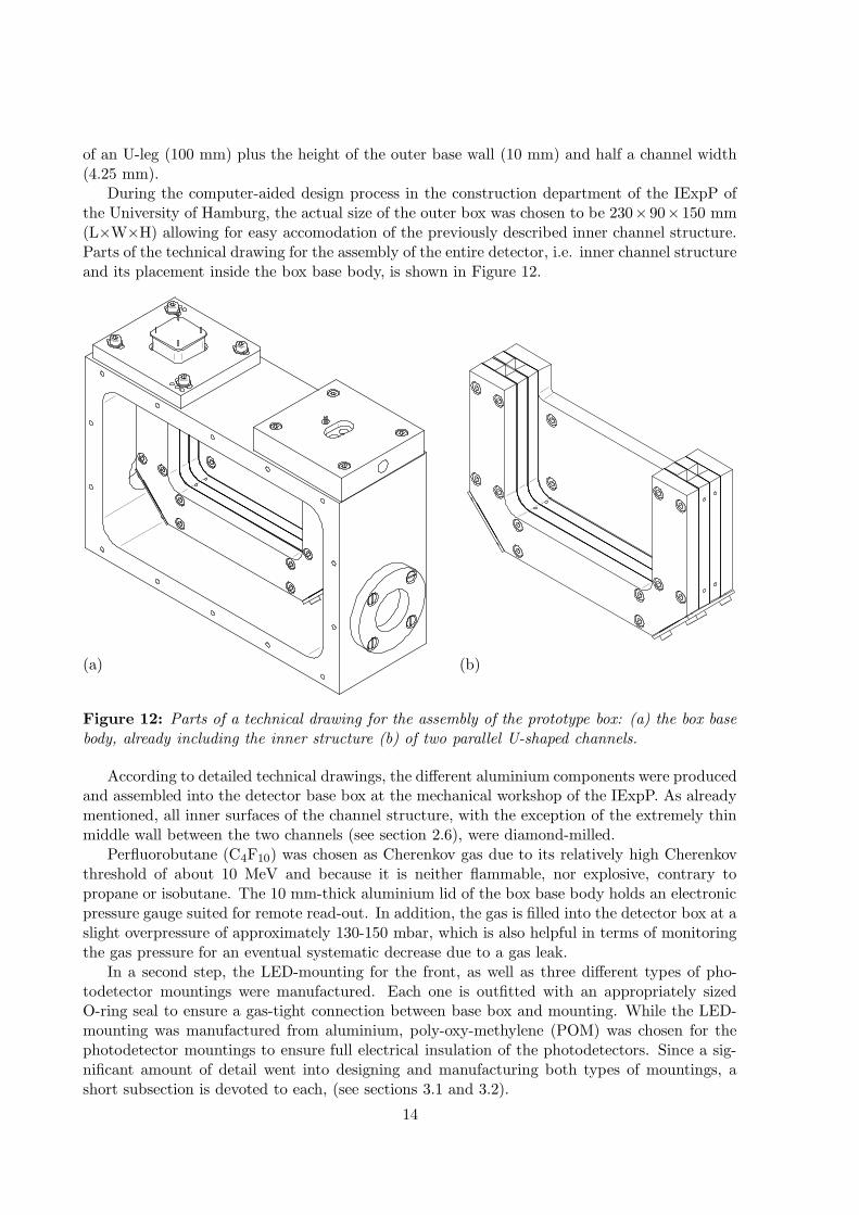
During the computer-aided design process in the construction department of the IExpP ofthe University of Hamburg, the actual size of the outer box was chosen to be 230×90×150 mm(L×W×H) allowing for easy accomodation of the previously described inner channel structure.Parts of the technical drawing for the assembly of the entire detector, i.e. inner channel structureand its placement inside the box base body, is shown in Figure 12.

(a) (b)

Figure 12: Parts of a technical drawing for the assembly of the prototype box: (a) the box basebody, already including the inner structure (b) of two parallel U-shaped channels.

According to detailed technical drawings, the different aluminium components were producedand assembled into the detector base box at the mechanical workshop of the IExpP. As alreadymentioned, all inner surfaces of the channel structure, with the exception of the extremely thinmiddle wall between the two channels (see section 2.6), were diamond-milled.

Perfluorobutane (C4F10) was chosen as Cherenkov gas due to its relatively high Cherenkovthreshold of about 10 MeV and because it is neither flammable, nor explosive, contrary topropane or isobutane. The 10 mm-thick aluminium lid of the box base body holds an electronicpressure gauge suited for remote read-out. In addition, the gas is filled into the detector box at aslight overpressure of approximately 130-150 mbar, which is also helpful in terms of monitoringthe gas pressure for an eventual systematic decrease due to a gas leak.

In a second step, the LED-mounting for the front, as well as three different types of pho-todetector mountings were manufactured. Each one is outfitted with an appropriately sizedO-ring seal to ensure a gas-tight connection between base box and mounting. While the LED-mounting was manufactured from aluminium, poly-oxy-methylene (POM) was chosen for thephotodetector mountings to ensure full electrical insulation of the photodetectors. Since a sig-nificant amount of detail went into designing and manufacturing both types of mountings, ashort subsection is devoted to each, (see sections 3.1 and 3.2).

14

3.1 Photodetectors and their mountings

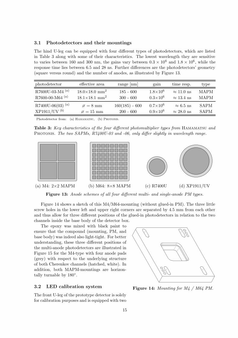
The hind U-leg can be equipped with four different types of photodetectors, which are listedin Table 3 along with some of their characteristics. The lowest wavelength they are sensitiveto varies between 160 and 300 nm, the gains vary between 0.3 × 106 and 1.8 × 106, while theresponse time lies between 6.5 and 28 ns. Further differences are the photodetectors’ geometry(square versus round) and the number of anodes, as illustrated by Figure 13.

photodetector effective area range [nm] gain time resp. type

R7600U-03-M4 (a) 18.0×18.0 mm2 185 - 600 1.8×106 ≈ 11.0 ns MAPM

R7600-00-M64 (a) 18.1×18.1 mm2 300 - 600 0.3×106 ≈ 13.4 ns MAPM

R7400U-06(03) (a) � = 8 mm 160(185) - 600 0.7×106 ≈ 6.5 ns SAPM

XP1911/UV (b) � = 15 mm 200 - 600 0.9×106 ≈ 28.0 ns SAPM

Photodetector from: (a) Hamamatsu, (b) Photonis.

Table 3: Key characteristics of the four different photomultiplier types from Hamamatsu andPhotonis. The two SAPMs, R7400U-03 and -06, only differ slightly in wavelength range.

(a) M4: 2×2 MAPM (b) M64: 8×8 MAPM (c) R7400U (d) XP1911/UV

Figure 13: Anode schemes of all four different multi- and single-anode PM types.

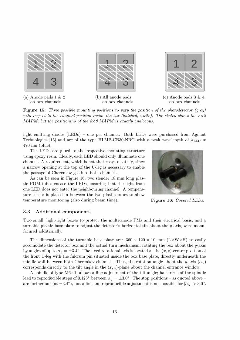
Figure 14 shows a sketch of this M4/M64-mounting (without glued-in PM). The three littlescrew holes in the lower left and upper right corners are separated by 4.5 mm from each otherand thus allow for three different positions of the glued-in photodetectors in relation to the twochannels inside the base body of the detector box.

Figure 14: Mounting for M4 / M64 PM.

The epoxy was mixed with black paint toensure that the compound (mounting, PM, andbase body) was indeed also light-tight. For betterunderstanding, these three different positions ofthe multi-anode photodetectors are illustrated inFigure 15 for the M4-type with four anode pads(grey) with respect to the underlying structureof both Cherenkov channels (hatched, white). Inaddition, both MAPM-mountings are horizon-tally turnable by 180◦.

3.2 LED calibration system

The front U-leg of the prototype detector is solelyfor calibration purposes and is equipped with two

15

1 2

34

1 2

34

1 2

34(a) Anode pads 1 & 2

on box channels(b) All anode pads

on box channels(c) Anode pads 3 & 4

on box channels

Figure 15: Three possible mounting positions to vary the position of the photodetector (grey)with respect to the channel position inside the box (hatched, white). The sketch shows the 2×2MAPM, but the positioning of the 8×8 MAPM is exactly analogous.

light emitting diodes (LEDs) – one per channel. Both LEDs were purchased from AgilantTechnologies [15] and are of the type HLMP-CB30-NRG with a peak wavelength of λLED ≈470 nm (blue).

Figure 16: Covered LEDs.

The LEDs are glued to the respective mounting structureusing epoxy resin. Ideally, each LED should only illuminate onechannel. A requirement, which is not that easy to satisfy, sincea narrow opening at the top of the U-leg is necessary to enablethe passage of Cherenkov gas into both channels.

As can be seen in Figure 16, two slender 18 mm long plas-tic POM-tubes encase the LEDs, ensuring that the light fromone LED does not enter the neighbouring channel. A tempera-ture sensor is placed in between the two plastic tubes to allowtemperature monitoring (also during beam time).

3.3 Additional components

Two small, light-tight boxes to protect the multi-anode PMs and their electrical basis, and aturnable plastic base plate to adjust the detector’s horizontal tilt about the y-axis, were manu-facured additionally.

The dimensions of the turnable base plate are: 360 × 120 × 10 mm (L×W×H) to easilyaccomodate the detector box and the actual turn mechanism, rotating the box about the y-axisby angles of up to αy = ±3.4◦. The fixed rotational axis is located at the (x, z)-centre position ofthe front U-leg with the fulcrum pin situated inside the box base plate, directly underneath themiddle wall between both Cherenkov channels. Thus, the rotation angle about the y-axis (αy)corresponds directly to the tilt angle in the (x, z)-plane about the channel entrance window.

A spindle of type M6×1, allows a fine adjustment of the tilt angle; half turns of the spindlelead to reproducible steps of 0.125◦ between αy = ±3.0◦. The stop positions – as quoted above –are further out (at ±3.4◦), but a fine and reproducible adjustment is not possible for |αy| > 3.0◦.

16

4 Functional tests and first testbeam results

After the assembly of the entire prototype, the detector was set up in the laboratory and filledwith the Cherenkov gas C4F10 at a slight overpressure of about 140 mbar. A relative barometerwas connected to the slow control and readout electronics which can be controlled remotely viaa desktop PC.

The detector system proved to be gas-tight, although frequent changes to the setup pre-vented a monitoring of the gas pressure for time periods longer than two weeks. Nevertheless,no systematic decrease in the gas pressure was observed. Only slight fluctuations were seen,depending on the actual atmospheric pressure, due to the initial overpressure with respect tothe atmospheric pressure.

4.1 Testbeam at ELSA: setup and first signals

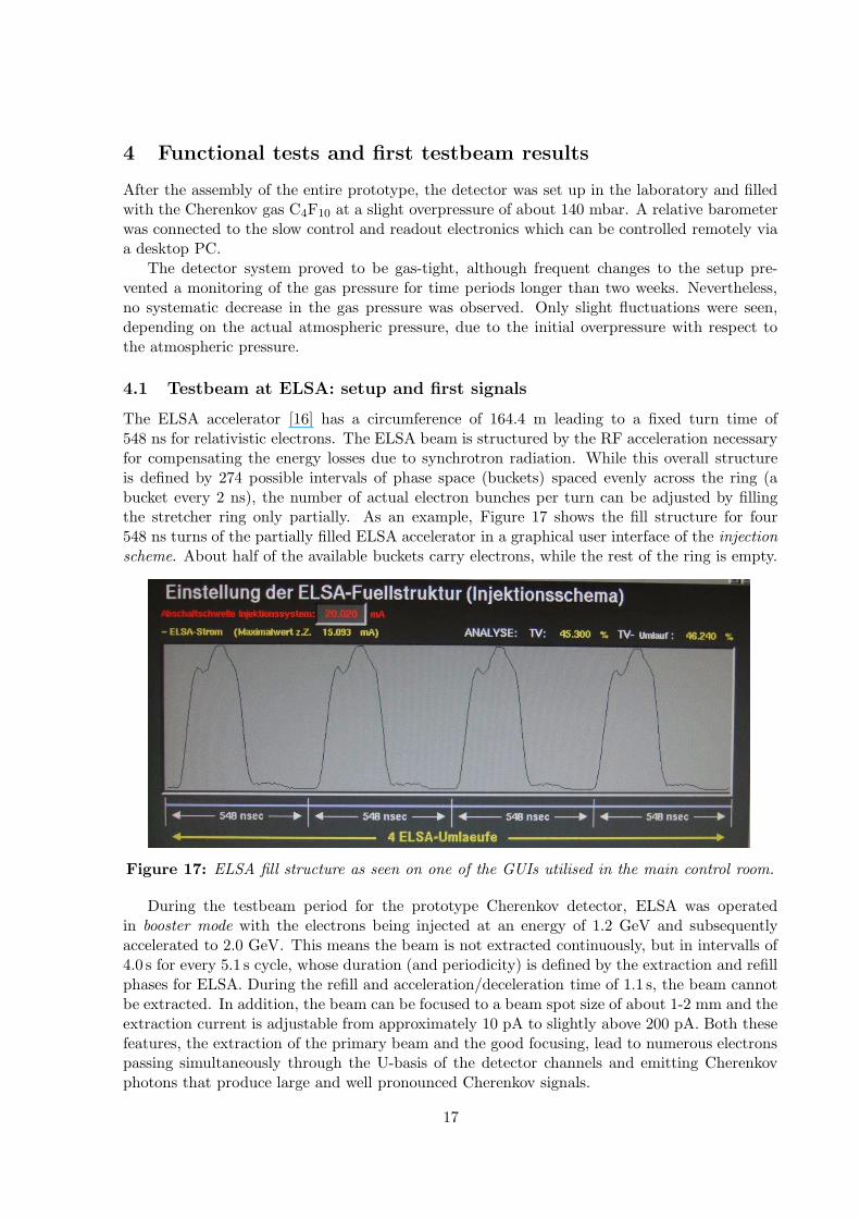
The ELSA accelerator [16] has a circumference of 164.4 m leading to a fixed turn time of548 ns for relativistic electrons. The ELSA beam is structured by the RF acceleration necessaryfor compensating the energy losses due to synchrotron radiation. While this overall structureis defined by 274 possible intervals of phase space (buckets) spaced evenly across the ring (abucket every 2 ns), the number of actual electron bunches per turn can be adjusted by fillingthe stretcher ring only partially. As an example, Figure 17 shows the fill structure for four548 ns turns of the partially filled ELSA accelerator in a graphical user interface of the injectionscheme. About half of the available buckets carry electrons, while the rest of the ring is empty.

Figure 17: ELSA fill structure as seen on one of the GUIs utilised in the main control room.

During the testbeam period for the prototype Cherenkov detector, ELSA was operatedin booster mode with the electrons being injected at an energy of 1.2 GeV and subsequentlyaccelerated to 2.0 GeV. This means the beam is not extracted continuously, but in intervalls of4.0 s for every 5.1 s cycle, whose duration (and periodicity) is defined by the extraction and refillphases for ELSA. During the refill and acceleration/deceleration time of 1.1 s, the beam cannotbe extracted. In addition, the beam can be focused to a beam spot size of about 1-2 mm and theextraction current is adjustable from approximately 10 pA to slightly above 200 pA. Both thesefeatures, the extraction of the primary beam and the good focusing, lead to numerous electronspassing simultaneously through the U-basis of the detector channels and emitting Cherenkovphotons that produce large and well pronounced Cherenkov signals.

17

Since no specific triggers were employed, the beam clock signal was looped through a func-tion generator which was used to provide the necessary gate for the QDC. Furthermore, byusing the function generator, the gate width could also be easily adjusted from 100 ns to 480 nsdepending on how many of the ELSA buckets were actually filled with electrons. The gate widthwas adjusted such that the detector prototype integrated all electron bunches of one completeELSA turn, since it was impossible to resolve the substructure of 2 ns-bunches. The expectedaverage number of electrons per ELSA turn is estimated from the extraction current (averagedover 100 ms, i.e. multiple turns) multiplied by the turn-time (548 ns) and divided by the ele-mentary charge. Hence, for an extraction current varying in between 10 pA and 200 pA, theaverage number of electrons traversing the detector U-basis varies from about 30 to 680 elec-trons, respectively. In comparison, up to 200 electrons per Compton interaction are expected inthe most populated channel of a polarimeter Cherenkov detector at the ILC.

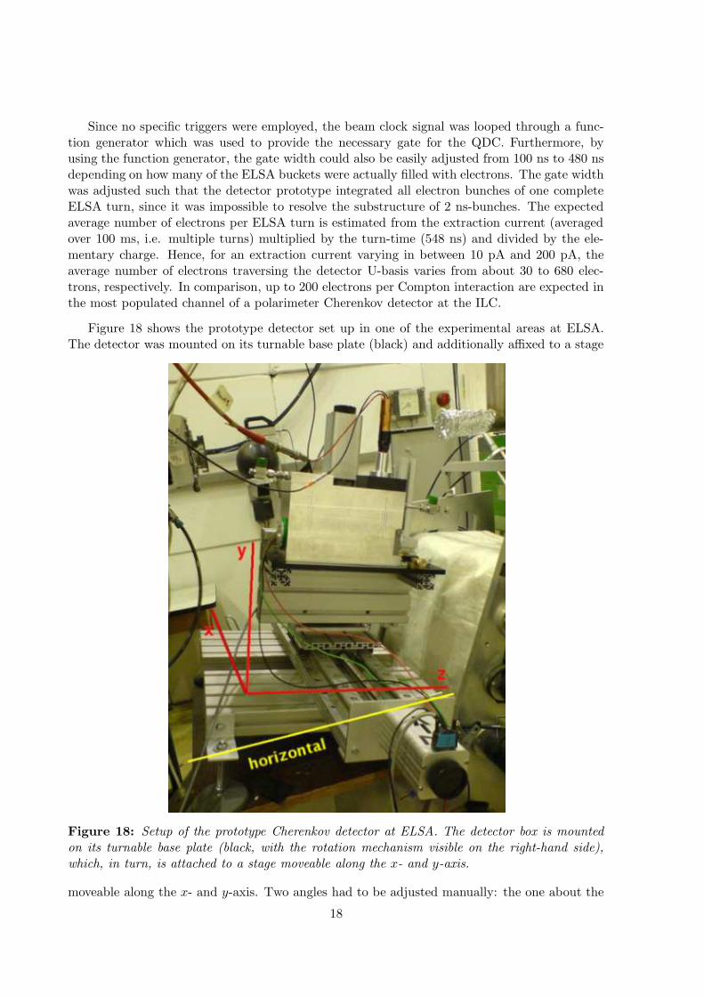
Figure 18 shows the prototype detector set up in one of the experimental areas at ELSA.The detector was mounted on its turnable base plate (black) and additionally affixed to a stage

Figure 18: Setup of the prototype Cherenkov detector at ELSA. The detector box is mountedon its turnable base plate (black, with the rotation mechanism visible on the right-hand side),which, in turn, is attached to a stage moveable along the x- and y-axis.

moveable along the x- and y-axis. Two angles had to be adjusted manually: the one about the

18

x-axis (αx) defining a tilt in the (y, z)-plane and the one about the z-axis (αz) corresponding toa tilt in the (x, y)-plane orthogonal to the beam axis. While the latter was adjusted to αz ≈ 0◦

using a simple water-level, the former tilt angle (about the x-axis) was very difficult to adjust,since the detector had to be positioned at an angle of about αx ≈ 7.5◦...7.8◦ with respect to thehorizontal to match the downwards slope of the electron beam line1.

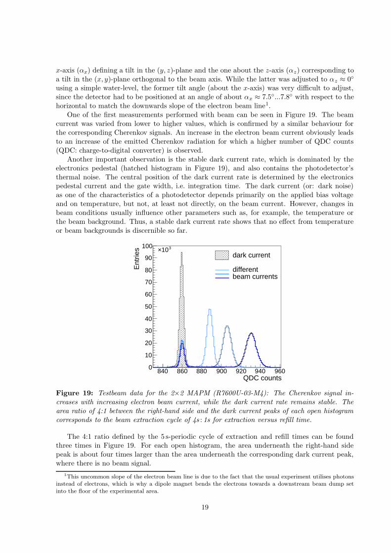
One of the first measurements performed with beam can be seen in Figure 19. The beamcurrent was varied from lower to higher values, which is confirmed by a similar behaviour forthe corresponding Cherenkov signals. An increase in the electron beam current obviously leadsto an increase of the emitted Cherenkov radiation for which a higher number of QDC counts(QDC: charge-to-digital converter) is observed.

Another important observation is the stable dark current rate, which is dominated by theelectronics pedestal (hatched histogram in Figure 19), and also contains the photodetector’sthermal noise. The central position of the dark current rate is determined by the electronicspedestal current and the gate width, i.e. integration time. The dark current (or: dark noise)as one of the characteristics of a photodetector depends primarily on the applied bias voltageand on temperature, but not, at least not directly, on the beam current. However, changes inbeam conditions usually influence other parameters such as, for example, the temperature orthe beam background. Thus, a stable dark current rate shows that no effect from temperatureor beam backgrounds is discernible so far.

QDC counts840 860 880 900 920 940 960

Ent

ries

0

10

20

30

40

50

60

70

80

90

100 310×dark current

differentbeam currents

Figure 19: Testbeam data for the 2×2 MAPM (R7600U-03-M4): The Cherenkov signal in-creases with increasing electron beam current, while the dark current rate remains stable. Thearea ratio of 4:1 between the right-hand side and the dark current peaks of each open histogramcorresponds to the beam extraction cycle of 4s : 1s for extraction versus refill time.

The 4:1 ratio defined by the 5 s-periodic cycle of extraction and refill times can be foundthree times in Figure 19. For each open histogram, the area underneath the right-hand sidepeak is about four times larger than the area underneath the corresponding dark current peak,where there is no beam signal.

1This uncommon slope of the electron beam line is due to the fact that the usual experiment utilises photonsinstead of electrons, which is why a dipole magnet bends the electrons towards a downstream beam dump setinto the floor of the experimental area.

19

4.2 Prototype alignment

Since it is nearly impossible to properly align the detector prototype with respect to the electronbeam line “by eye”, the position was carefully adjusted using the Cherenkov data itself. An ap-proach which is especially useful keeping in mind that the alignment of the real ILC-polarimeterCherenkov detector will eventually also have to be fine tuned this way.

After each exchange of photodetectors the first few runs are dedicated to find the correctoperating (or: bias) voltage for the new PM, which allows to distinguish Cherenkov signals fromthe dark current peak even for low electron beam currents of about 20 pA, and also keep a linearresponse to high beam currents.

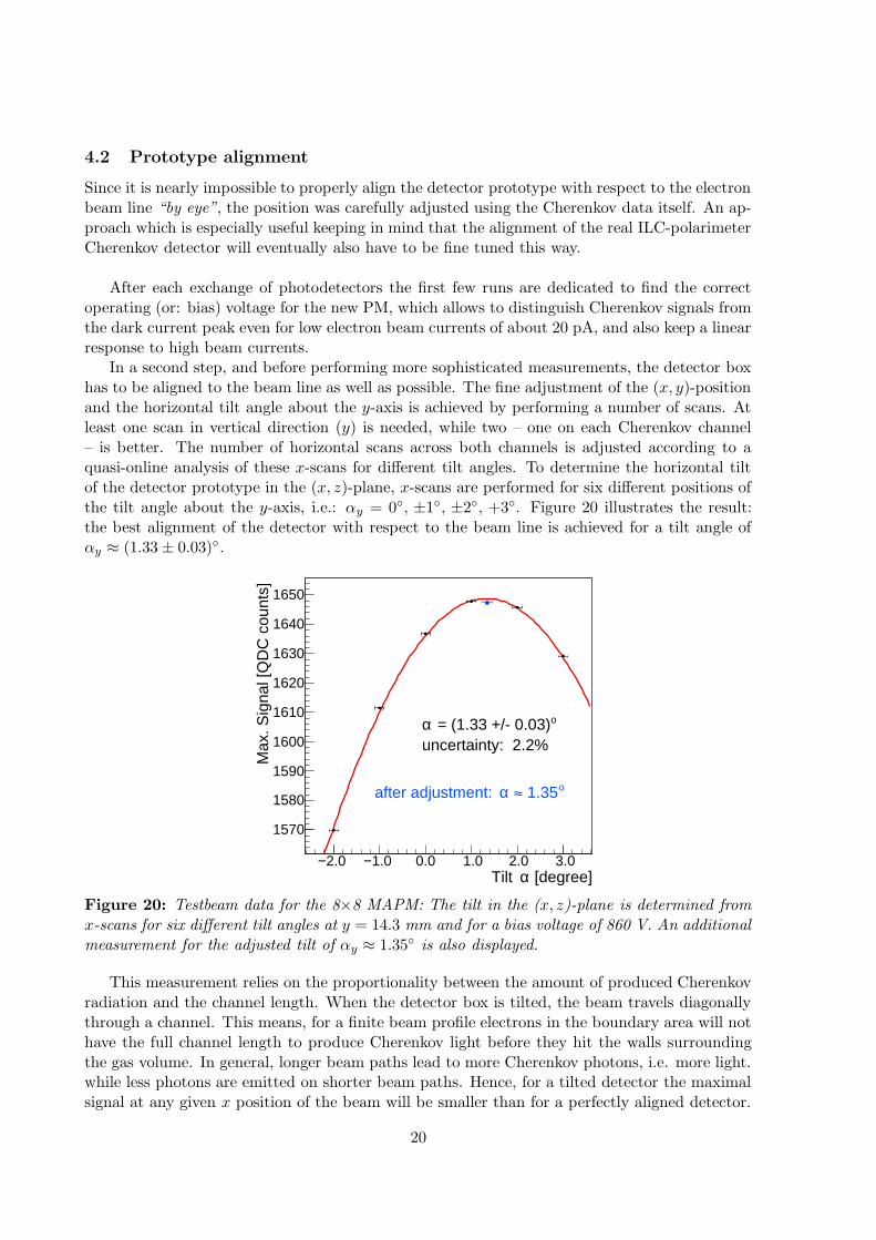
In a second step, and before performing more sophisticated measurements, the detector boxhas to be aligned to the beam line as well as possible. The fine adjustment of the (x, y)-positionand the horizontal tilt angle about the y-axis is achieved by performing a number of scans. Atleast one scan in vertical direction (y) is needed, while two – one on each Cherenkov channel– is better. The number of horizontal scans across both channels is adjusted according to aquasi-online analysis of these x-scans for different tilt angles. To determine the horizontal tiltof the detector prototype in the (x, z)-plane, x-scans are performed for six different positions ofthe tilt angle about the y-axis, i.e.: αy = 0◦, ±1◦, ±2◦, +3◦. Figure 20 illustrates the result:the best alignment of the detector with respect to the beam line is achieved for a tilt angle ofαy ≈ (1.33 ± 0.03)◦.

Tilt [degree]α−2.0 −1.0 0.0 1.0 2.0 3.0

Max

. Sig

nal [

QD

C c

ount

s]

1570

1580

1590

1600

1610

1620

1630

1640

1650

α = (1.33 +/- 0.03) o

uncertainty: 2.2%

after adjustment: α ~ 1.35~o

Figure 20: Testbeam data for the 8×8 MAPM: The tilt in the (x, z)-plane is determined fromx-scans for six different tilt angles at y = 14.3 mm and for a bias voltage of 860 V. An additionalmeasurement for the adjusted tilt of αy ≈ 1.35◦ is also displayed.

This measurement relies on the proportionality between the amount of produced Cherenkovradiation and the channel length. When the detector box is tilted, the beam travels diagonallythrough a channel. This means, for a finite beam profile electrons in the boundary area will nothave the full channel length to produce Cherenkov light before they hit the walls surroundingthe gas volume. In general, longer beam paths lead to more Cherenkov photons, i.e. more light.while less photons are emitted on shorter beam paths. Hence, for a tilted detector the maximalsignal at any given x position of the beam will be smaller than for a perfectly aligned detector.

20

Thus, the following procedure has been adopted: at different angles, the detector front faceis scanned horizontally by the electron beam. The x position for which the highest signal isobserved is then compared for all angles.

Using the turnable base plate with the fine adjusting rotation mechanism and the abovemethod to determine the horizontal tilt, the positioning in the (x, z)-plane could be improvedtremendously from ∆αy ? 3◦ to an accuracy of ∆αy > 0.1◦.

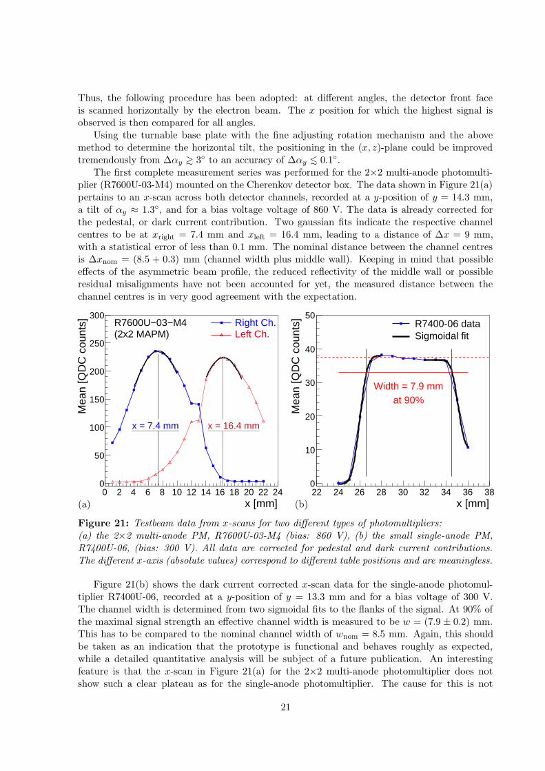
The first complete measurement series was performed for the 2×2 multi-anode photomulti-plier (R7600U-03-M4) mounted on the Cherenkov detector box. The data shown in Figure 21(a)pertains to an x-scan across both detector channels, recorded at a y-position of y = 14.3 mm,a tilt of αy ≈ 1.3◦, and for a bias voltage voltage of 860 V. The data is already corrected forthe pedestal, or dark current contribution. Two gaussian fits indicate the respective channelcentres to be at xright = 7.4 mm and xleft = 16.4 mm, leading to a distance of ∆x = 9 mm,with a statistical error of less than 0.1 mm. The nominal distance between the channel centresis ∆xnom = (8.5 + 0.3) mm (channel width plus middle wall). Keeping in mind that possibleeffects of the asymmetric beam profile, the reduced reflectivity of the middle wall or possibleresidual misalignments have not been accounted for yet, the measured distance between thechannel centres is in very good agreement with the expectation.

x [mm]0 2 4 6 8 10 12 14 16 18 20 22 24

Mea

n [Q

DC

cou

nts]

0

50

100

150

200

250

300R7600U−03−M4(2x2 MAPM)

Right Ch.Left Ch.

x = 7.4 mm x = 16.4 mm

x [mm]22 24 26 28 30 32 34 36 38

Mea

n [Q

DC

cou

nts]

0

10

20

30

40

50R7400-06 dataSigmoidal fit

Width = 7.9 mmat 90%

(a) (b)

Figure 21: Testbeam data from x-scans for two different types of photomultipliers:(a) the 2×2 multi-anode PM, R7600U-03-M4 (bias: 860 V), (b) the small single-anode PM,R7400U-06, (bias: 300 V). All data are corrected for pedestal and dark current contributions.The different x-axis (absolute values) correspond to different table positions and are meaningless.

Figure 21(b) shows the dark current corrected x-scan data for the single-anode photomul-tiplier R7400U-06, recorded at a y-position of y = 13.3 mm and for a bias voltage of 300 V.The channel width is determined from two sigmoidal fits to the flanks of the signal. At 90% ofthe maximal signal strength an effective channel width is measured to be w = (7.9 ± 0.2) mm.This has to be compared to the nominal channel width of wnom = 8.5 mm. Again, this shouldbe taken as an indication that the prototype is functional and behaves roughly as expected,while a detailed quantitative analysis will be subject of a future publication. An interestingfeature is that the x-scan in Figure 21(a) for the 2×2 multi-anode photomultiplier does notshow such a clear plateau as for the single-anode photomultiplier. The cause for this is not

21

precisely known. As one of the most likely reasons, the influence from an ellipsoidal elongatedbeam profile is currently being investigated in detail. Once the effect can be reproduced, it ispossible to deconvolute the data with a simulated profile and thus correct for the ELSA beamprofile.

The absolute x-values (x-axis) are of no importance other than to indicate the position ofthe remote-controlled moveable stage.

4 56732

z

x

y

Figure 22: Anode readout configura-tion for the 8×8 multi-anode PM.

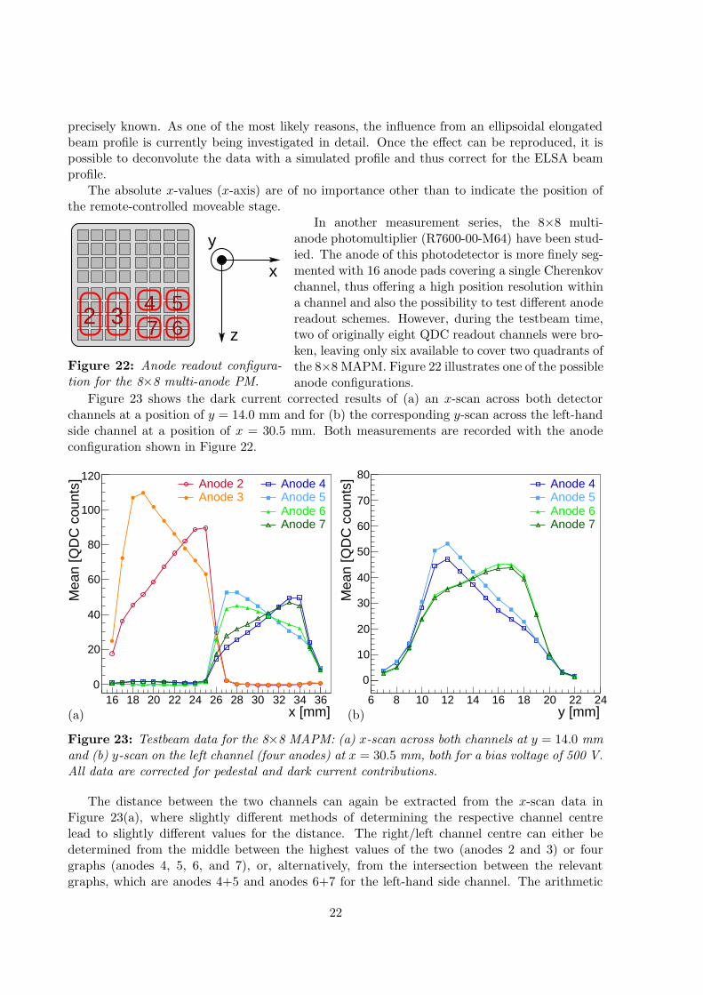
In another measurement series, the 8×8 multi-anode photomultiplier (R7600-00-M64) have been stud-ied. The anode of this photodetector is more finely seg-mented with 16 anode pads covering a single Cherenkovchannel, thus offering a high position resolution withina channel and also the possibility to test different anodereadout schemes. However, during the testbeam time,two of originally eight QDC readout channels were bro-ken, leaving only six available to cover two quadrants ofthe 8×8 MAPM. Figure 22 illustrates one of the possibleanode configurations.

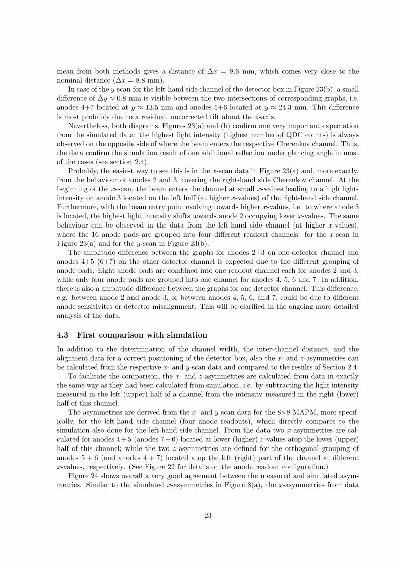
Figure 23 shows the dark current corrected results of (a) an x-scan across both detectorchannels at a position of y = 14.0 mm and for (b) the corresponding y-scan across the left-handside channel at a position of x = 30.5 mm. Both measurements are recorded with the anodeconfiguration shown in Figure 22.

x [mm]16 18 20 22 24 26 28 30 32 34 36

Mea

n [Q

DC

cou

nts]

0

20

40

60

80

100

120Anode 2Anode 3

Anode 4Anode 5Anode 6Anode 7

y [mm]6 8 10 12 14 16 18 20 22 24

Mea

n [Q

DC

cou

nts]

0

10

20

30

40

50

60

70

80Anode 4Anode 5Anode 6Anode 7

(a) (b)

Figure 23: Testbeam data for the 8×8 MAPM: (a) x-scan across both channels at y = 14.0 mmand (b) y-scan on the left channel (four anodes) at x = 30.5 mm, both for a bias voltage of 500 V.All data are corrected for pedestal and dark current contributions.

The distance between the two channels can again be extracted from the x-scan data inFigure 23(a), where slightly different methods of determining the respective channel centrelead to slightly different values for the distance. The right/left channel centre can either bedetermined from the middle between the highest values of the two (anodes 2 and 3) or fourgraphs (anodes 4, 5, 6, and 7), or, alternatively, from the intersection between the relevantgraphs, which are anodes 4+5 and anodes 6+7 for the left-hand side channel. The arithmetic

22

mean from both methods gives a distance of ∆x = 8.6 mm, which comes very close to thenominal distance (∆x = 8.8 mm).

In case of the y-scan for the left-hand side channel of the detector box in Figure 23(b), a smalldifference of ∆y ≈ 0.8 mm is visible between the two intersections of corresponding graphs, i.e.anodes 4+7 located at y ≈ 13.5 mm and anodes 5+6 located at y ≈ 24.3 mm. This differenceis most probably due to a residual, uncorrected tilt about the z-axis.

Nevertheless, both diagrams, Figures 23(a) and (b) confirm one very important expectationfrom the simulated data: the highest light intensity (highest number of QDC counts) is alwaysobserved on the opposite side of where the beam enters the respective Cherenkov channel. Thus,the data confirm the simulation result of one additional reflection under glancing angle in mostof the cases (see section 2.4).

Probably, the easiest way to see this is in the x-scan data in Figure 23(a) and, more exactly,from the behaviour of anodes 2 and 3, covering the right-hand side Cherenkov channel. At thebeginning of the x-scan, the beam enters the channel at small x-values leading to a high light-intensity on anode 3 located on the left half (at higher x-values) of the right-hand side channel.Furthermore, with the beam entry point evolving towards higher x-values, i.e. to where anode 3is located, the highest light intensity shifts towards anode 2 occupying lower x-values. The samebehaviour can be observed in the data from the left-hand side channel (at higher x-values),where the 16 anode pads are grouped into four different readout channels: for the x-scan inFigure 23(a) and for the y-scan in Figure 23(b).

The amplitude difference between the graphs for anodes 2+3 on one detector channel andanodes 4+5 (6+7) on the other detector channel is expected due to the different grouping ofanode pads. Eight anode pads are combined into one readout channel each for anodes 2 and 3,while only four anode pads are grouped into one channel for anodes 4, 5, 6 and 7. In addition,there is also a amplitude difference between the graphs for one detector channel. This difference,e.g. between anode 2 and anode 3, or between anodes 4, 5, 6, and 7, could be due to differentanode sensitivites or detector misalignment. This will be clarified in the ongoing more detailedanalysis of the data.

4.3 First comparison with simulation

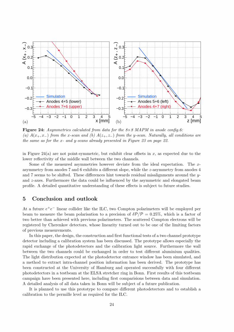
In addition to the determination of the channel width, the inter-channel distance, and thealignment data for a correct positioning of the detector box, also the x- and z-asymmetries canbe calculated from the respective x- and y-scan data and compared to the results of Section 2.4.

To facilitate the comparison, the x- and z-asymmetries are calculated from data in exactlythe same way as they had been calculated from simulation, i.e. by subtracting the light intensitymeasured in the left (upper) half of a channel from the intensity measured in the right (lower)half of this channel.

The asymmetries are derived from the x- and y-scan data for the 8×8 MAPM, more specif-ically, for the left-hand side channel (four anode readouts), which directly compares to thesimulation also done for the left-hand side channel. From the data two x-asymmetries are cal-culated for anodes 4+5 (anodes 7+6) located at lower (higher) z-values atop the lower (upper)half of this channel; while the two z-asymmetries are defined for the orthogonal grouping ofanodes 5 + 6 (and anodes 4 + 7) located atop the left (right) part of the channel at differentx-values, respectively. (See Figure 22 for details on the anode readout configuration.)

Figure 24 shows overall a very good agreement between the measured and simulated asym-metries. Similar to the simulated x-asymmetries in Figure 8(a), the x-asymmetries from data

23

x [mm]−5 −4 −3 −2 −1 0 1 2 3 4 5

A (

x ,

x

)+

−

−0.3

−0.2

−0.1

0.0

0.1

0.2

0.3

SimulationAnodes 4+5 (lower)Anodes 7+6 (upper)

z [mm]−5 −4 −3 −2 −1 0 1 2 3 4 5

A (

z ,

z

)+

−

−0.3

−0.2

−0.1

0.0

0.1

0.2

0.3

SimulationAnodes 5+6 (left)Anodes 4+7 (right)

(a) (b)

Figure 24: Asymmetries calculated from data for the 8×8 MAPM in anode config.6:(a) A(x+, x−) from the x-scan and (b) A(z+, z−) from the y-scan. Naturally, all conditions arethe same as for the x- and y-scans already presented in Figure 23 on page 22.

in Figure 24(a) are not point-symmetric, but exhibit clear offsets in x, as expected due to thelower reflectivity of the middle wall between the two channels.

Some of the measured asymmetries however deviate from the ideal expectation. The x-asymmetry from anodes 7 and 6 exhibits a different slope, while the z-asymmetry from anodes 4and 7 seems to be shifted. These differences hint towards residual misalignments around the y-and z-axes. Furthermore the data could be influenced by the asymmetric and elongated beamprofile. A detailed quantitative understanding of these effects is subject to future studies.

5 Conclusion and outlook

At a future e+e− linear collider like the ILC, two Compton polarimeters will be employed perbeam to measure the beam polarisation to a precision of δP/P = 0.25%, which is a factor oftwo better than achieved with previous polarimeters. The scattered Compton electrons will beregistered by Cherenkov detectors, whose linearity turned out to be one of the limiting factorsof previous measurements.

In this paper, the design, the construction and first functional tests of a two channel prototypedetector including a calibration system has been discussed. The prototype allows especially therapid exchange of the photodetectors and the calibration light source. Furthermore the wallbetween the two channels could be exchanged in order to test different aluminium qualities.The light distribution expected at the photodetector entrance window has been simulated, anda method to extract intra-channel position information has been derived. The prototype hasbeen constructed at the University of Hamburg and operated successfully with four differentphotodetectors in a testbeam at the ELSA stretcher ring in Bonn. First results of this testbeamcampaign have been presented here, including first comparisions between data and simulation.A detailed analysis of all data taken in Bonn will be subject of a future publication.

It is planned to use this prototype to compare different photodetectors and to establish acalibration to the permille level as required for the ILC.

24

Acknowledgements

We thank the design and technical construction team of the Institut fur Experimentalphysikof the University of Hamburg, B. Frensche and J. Pelz, as well as the head of the mechanicalworkshop, S. Fleig, and his entire team for their competent work.

The authors are grateful to W. Hillert, F. Frommberger and the entire ELSA-team for theirsupport during the testbeam period, for realising rather special beam requests and for manyhelpful discussions concerning a multitude of different ELSA technicalities. Further thanks goto K. Desch, J. Kaminski, D. Elsner, and many others for help and support with the planningand setup before, during, and after the two weeks in Bonn.

The authors acknowledge the financial support of the Deutsche Forschungsgemeinschaft inthe DFG project Li 1560/1-1 and of the HGF-alliance.

References

[1] ILC Global Design Effort and World Wide Study, “International Linear Collider Reference Design Report- Volume 2: Physics at the ILC,” Editors: A. Djouadi, J. Lykken, K. Monig, Y. Okada, M. Oreglia, andS. Yamashita, “International Linear Collider Reference Design Report - Volume 3: Accelerator”, Editors:N. Phinney, N. Toge, and N. Walker, August 2007.

[2] G.A. Moortgat-Pick et al., “The Role of Polarised Positrons and Electrons in Revealing Fundamental Inter-actions at the Linear Collider,” Phys. Rept. 460 (2008) 131, [arXiv:hep-ph/0507011].

[3] [ALEPH, DELPHI, L3, OPAL and SLD Collaborations], “Precision electroweak measurements on the Zresonance,” Phys. Rept. 427 (2006) 257; [arXiv:hep-ex/0509008].

[4] S. Boogert, A.F. Hartin, M. Hildreth, D. Kafer, J List, T. Maruyama, K. Monig, K.C. Moffeit, G. Moortgat-Pick, S. Riemann, H.J. Schreiber, P. Schuler, E. Torrence, M. Woods, “Polarimeters and Energy Spectrom-eters for the ILC Beam Delivery System,” JINST 4 (2009) P10015. [arXiv:0904.0122v2 physics.ins-det].

[5] C. Bartels, C. Helebrant, D. Kafer and J. List, “Compton Cherenkov Detector Development for ILC Po-larimetry,” arXiv:0902.3221 [physics.ins-det]. To be published in the proceedings of the International LinearCollider Workshop 2008 (LCWS’08 and ILC’08), Chicago, U.S.A., November, 2008

[6] V. Gharibyan, N. Meyners, and K.P. Schuler, TESLA Report 2001-23, Part III, LC-DET-2001-047, DESY,February 2001; DESY 2001-011, March 2001

[7] The GEANT4 Collaboration, “GEANT4 – A Simulation Toolkit,” Nucl. Instrum. Meth. Phys. Res. A 506,Issue 3 (2003), 250-303; The GEANT4 Collaboration, “GEANT4 Developments and Applications,” IEEETrans. Nucl. Science 53 No. 1 (2006), 270-278; ISSN: 0018-9499

[8] C. Helebrant, D. Kafer, J. List, C. Bartels, Poster “Photodetector Studies and Prototype Simulation of aCherenkov Detector for an ILC Polarimeter,” IEEE 2008 Nuclear Science Symposium and Medical ImagingConference, Dresden, Germany, October, 2008.

[9] C. Helebrant, “Evaluation of different photodetector types for an ILC polarimeter,” accepted by Nucl.Instrum. Meth. Phys. Res. A http://dx.doi.org/10.1016/j.nima.2009.05.126

[10] C. Helebrant, “In Search of New Physics Using Polarisation — HERA and ILC,” Ph.D. Thesis, Universityof Hamburg, Hamburg, Germany, 2009.

[11] Hamamatsu Photonics K.K. http://www.hamamatsu.com

R7600U-03-M4 (2007): http://sales.hamamatsu.com/assets/pdf/parts_R/R5900U_R7600U_TPMH1291E03.pdfR7600-00-M64 (2006): http://sales.hamamatsu.com/index.php?id=13195917

R7400U-06(03) (2004): http://sales.hamamatsu.com/assets/pdf/parts_R/R7400U_TPMH1204E07.pdf

[12] PerkinElmer, http://www.perkinelmer.com Lambda 800 Spectrometerhttp://las.perkinelmer.com/Catalog/default.htm?CategoryID=Lambda+800+Spectrometer

[13] GoodFellow GmbH, Germany, https://www.goodfellow.com

Aluminium foil: AL000601 (thickness: 0.15 mm, purity: 99.0%, hardness: hard)

[14] Photonis USA, http://www.photonis.com

XP1911/UV (1999): http://www.photonis.com/upload/industryscience/pdf/pmt/XP1911UV.pdf

25

[15] Agilant Technologies, LED, T-1 3/4 (5 mm) Precision Optical Performance InGaN Blue and Green Lamps,Technical Data (2002) available at: http://www.agilent.com

[16] W. Hillert, “The Bonn electron stretcher accelerator ELSA: Past and future,” Eur. Phys. J. A 28S1 (2006)139.

26