Design and automatic tuning of a motorcycle state … · Design and automatic tuning of a motorcycle state estimator ... weekly Friday night drinks, ... took me to Tunesia ...

Design and automatic tuning of a motorcycle state estimator

B.A.M. van Daal DCT 2009.025

Master’s thesis Coach: Dr. Ir. I.J.M. Besselink (TU/e)

Ir. S.T.H. Jansen (TNO)

Supervisor: Prof. Dr. H. Nijmeijer (TU/e) Committee: Prof. Dr. H. Nijmeijer (TU/e) Dr. Ir. I.J.M. Besselink (TU/e) Dr. Ir. T. Hofman (TU/e) Ir. S.T.H. Jansen (TNO) TNO Science & Industry Business Unit Automotive Department Integrated Safety Eindhoven University of Technology Department Mechanical Engineering Dynamics and Control Group Eindhoven, April, 2009

i

Abstract Measurement and evaluation of motorcycle handling behavior is challenging as it requires expensive sensor instrumentation, and the accuracy may be insufficient for control application. State estimation is a technique that combines measurements with a model representation that has been proven effective, however optimizing the state estimator settings is a laborious task. With a motorcycle state estimator real time information concerning the motions of a motorcycle can be obtained during driving. In the future, with this information a safety system can be designed.

This report focuses on the design and tuning of a motorcycle state estimator. The motorcycle state estimator comprises an analytical motorcycle model to estimate the motorcycle states, and an innovation to correct the estimations. TNO already developed a first version of a motorcycle state estimator. Tuning this state estimator requires a thorough knowledge of the analytical motorcycle model and is very time consuming. The objective of this investigation is to develop a structured method to design and automatically tune a motorcycle state estimator. Tuning the motorcycle state estimator requires knowledge of model deviations and noise on the measurement sensor signals. The tuning of the motorcycle state estimator can be automated by assuming a linear behavior of the motorcycle. For this, simplifications need to be done on the motorcycle model used in the TNO motorcycle state estimator. These simplifications do not noticeably result in a loss of accuracy, robustness or stability of the state estimator.

An automatic tuning routine is proposed to tune both the Kalman filter and the linear observer. The automatic tuning routine optimizes the settings for each of the two state estimators within one day (on a Pentium 2Ghz computer). For both the simulation model and the real motorcycle, the state estimators perform desirably accurate and robust. The Kalman filter and linear observer are validated on a broad set of reference measurements which comprise all types of maneuvers of both normal and limit handling driving. Results of the Kalman filter and linear observer are comparable to the TNO motorcycle state estimator results.

The automatic tuning routine is benchmarked with a second analytical motorcycle model with higher complexity. A Kalman filter and a linear observer are designed with this analytical motorcycle model. The automatic tuning routine is used to tune both the Kalman Filter and the linear observer for the real motorcycle. Again, for the same set of reference measurements, two robust state estimators are obtained, proving the potential of the automatic tuning routine as well as the linear observer.

ii

iii

Samenvatting Het meten en evalueren van motorfiets rijgedrag is uitdagend omdat een dure sensor instrumentatie benodigd is en de nauwkeurigheid onvoldoende kan zijn voor control applicaties. Toestand schatting is een techniek waarbij metingen gecombineerd worden met een model representatie. De kracht van deze techniek is bewezen, maar het optimaliseren van de instellingen is erg bewerkelijk. Met een motorfiets toestand schatter kan real-time informatie omtrent de bewegingen van de motorfiets tijdens het rijden worden vergaard. Met deze informatie kan een veiligheidssysteem ontwikkeld worden.

Dit rapport richt zich op het ontwerp en instellen van een motorfiets toestand schatter. De motorfiets toestand schatter bevat een analytisch motorfiets model om de toestanden van de motorfiets te schatten en een innovatieterm om de schattingen te corrigeren. TNO heeft reeds een eerste versie van een motorfiets toestand schatter ontwikkeld. Het optimaliseren van de instellingen van deze toestand schatter vereist een uitgebreide kennis van het analytisch motorfiets model en vergt erg veel tijd. Het doel van dit onderzoek is om een gestructureerde methode te ontwerpen om een motorfiets toestand schatter te ontwerpen en de instellingen te optimaliseren.

Het tunen van de motorfietstoestandschatter vereist kennis over de modelafwijkingen en ruis op de meetsignalen. Het tunen van de toestandschatter kan geautomatiseerd worden door lineair gedrag van de motorfiets aan te nemen. Hiervoor zijn enkele vereenvoudigingen nodig aan het motorfietsmodel welke in de TNO motorfietstoestandschatter is gebruikt. Deze vereenvoudigingen leiden niet tot een merkbaar verlies in nauwkeurigheid, robuustheid of stabiliteit van de toestandschatter.

Een automatische tuning routine is voorgesteld om zowel het Kalman filter als een lineaire waarnemer te tunen. De routine optimaliseert de instellingen voor elk van de twee toestandschatters binnen één dag (op een Pentium 2Ghz computer). Voor zowel een simulatiemodel als de echte motorfiets gedragen de toestandschatters zich voldoende nauwkeurig en robuust. Het Kalman filter en de lineaire waarnemer zijn gevalideerd op een grote set van referentiemetingen welke alle verschillende type manoeuvres bevat, zowel normale als extreme. Resultaten van het Kalman filter en de lineaire waarnemer zin vergelijkbaar met de TNO motorfietstoestandschatter.

Het automatisch ontwerp proces is getoetst voor het ontwerp van een tweetal toestandschatters waarbij een ander analytisch motorfiets model met een hogere complexiteit is geïmplementeerd. Zowel een Kalman filter als een lineaire waarnemer worden getuned met behulp van de automatische tuning routine. Ook met dit niet-lineaire model wordt, voor dezelfde set referentiemetingen, een tweetal robuuste motorfietstoestandschatters verkregen. Dit bewijst de potentie van zowel de automatisch tuning routine als van de lineaire waarnemer.

iv

v

Acknowledgements Last year at TNO, has been one of the most instructive years of my life, due to both positive and negative experiences. Everyone who contributed in this (especially the positive experiences) deserves a word of thanks. A special word of thanks goes to them who made it possible for me to complete the report which now lies in front of you. I would like to thank my supervisor and coaches Henk Nijmeijer, Sven Jansen and Igo Besselink for their guidance throughout my research and Theo Hofman for participating in my graduation committee. Their support with advice and comments during this research was very valuable. Remarkably Sven not only showed to be a coach, he also proved to be a successful trader. For instance, I got the opportunity to join the motorcycle tests in Idiada, Spain, in trade for preparatory work for these tests. Even more remarkable: in trade for characterizing the spring-damper characteristics of the Yamaha FJR1300 test motorcycle I received a nearly complete motorcycle. Sven, once again thanks for this. I would also like to thank my direct colleagues Roel and Erik, but also Bart, Hanno, Jos, Arjan, Willem and Bauke for their help and chitchats. Roel, success with Sam and a professional golf career. Erik, good luck with the Patrol, Mille and perhaps whenever you’ll get the opportunity an own company. Of course a special word of thanks goes to my parents, in first place because they made it possible for me to study at the Technical University of Eindhoven and secondly because of their unconditional support throughout my entire study. Without them this report probably would not have been realized. Pap en mam, enorm bedankt. Also my friends in Eindhoven and Bergeijk have been a great help for me. Bart, thanks for the weekly evaluations of our struggles during traineeship. Frank, thanks for accompanying me on the foreign motorcycle travels. Frank and David, thanks for the weekly Friday night drinks, schuppes. Last but definitely not least I would like to thank the coffee machine at TNO, the Yamaha FJR and the Yamaha XT. The coffee machine proved to be very helpful and highly effective during the afternoons and helped me to keep my attention to the work. Also a couple of informative discussions concerning my graduation work originated at the coffee machine. Thanks to the FJR for now and then liberating me from the on and on gazing to the computer screen. On the one hand for the repairs I needed to do, on the other hand for the test drives which I performed. Finally I would like to conclude my word of thanks by thanking the Yamaha XT from 1984, bought for 230 euro. The XT not only took me to Tunesia (and back), but also got me from Eindhoven to TNO Helmond daily, regardless of the weather conditions. The XT has proven to be a reliable partner. Don’t get confused by the lightness of this part of the report, from here on we will try to present the text more seriously and lift it to a higher academic level.

vi

1

Contents Summary i Samenvatting iii Acknowledgements v 1. Introduction................................................................................................................... 2

1.1 Background............................................................................................................... 2 1.2 Problem statement..................................................................................................... 3 1.3 Report outline............................................................................................................ 3

2. Literature survey .......................................................................................................... 4 2.1 Observers and state estimation.................................................................................. 4 2.2 Motorcycle dynamics................................................................................................ 8

3. Vehicle state estimator................................................................................................ 12 3.1 Car model................................................................................................................ 12 3.2 State estimator design ............................................................................................. 15 3.3 Simulations with state estimators............................................................................ 19 3.4 Summary................................................................................................................. 23

4. Optimized linear observer.......................................................................................... 24 4.1 Motivation and difference to conventional method................................................ 24 4.2 Optimization algorithm........................................................................................... 26 4.3 Matlab implementation ........................................................................................... 28 4.4 Summary................................................................................................................. 29

5. State estimator design for a virtual motorcycle ....................................................... 30 5.1 Automatic state estimator tuning ............................................................................ 31 5.2 Simulations with virtual motorcycle state estimators ............................................. 37 5.3 Summary................................................................................................................. 41

6. State estimator design for a real motorcycle ............................................................ 42 6.1 Automatic state estimator tuning ............................................................................ 42 6.2 Experiments with real motorcycle state estimators ................................................ 46 6.3 Benchmark .............................................................................................................. 52 6.4 Summary................................................................................................................. 54

7. Conclusions and recommendations ........................................................................... 55 7.1 Conclusions............................................................................................................. 55 7.2 Recommendations................................................................................................... 57

Bibliography .................................................................................................................... 59 A. Vehicle equations of motion ...................................................................................... 61 B. Gain matrices and closed loop pole locations .......................................................... 62 C. Matlab ......................................................................................................................... 64 D. Pacejka analytic motorcycle model .......................................................................... 66

2

1. Introduction 1.1 Background The number of motor vehicles has constantly grown during the last decades. As a result of the increased traffic density, more and more motorcycles are used to take over the tasks of a car; getting from A to B in a safe and comfortable way [1, 2]. For safety reasons and to satisfy the desires of the customers, motorcycles nowadays are equipped with electronic control systems. Systems as Antilock Braking System (ABS) and Traction Control System (TCS) are already securing the safety and comfort of the driver. The need for a system which enhances the safety of the driver during cornering grows with growing number of (fatal) accidents due to loss of control during cornering.

Safety during cornering can be secured when information about the motorcycle motions, the motorcycle states, is available. From the states for instance, tyre side slip angles and tyre lateral forces can be calculated. Too large side slip angles can be correlated to unsafe situations (in those cases, control systems may be activated).

Measuring all the states necessary for this evaluation is not an option for two reasons. First because this would require a very expensive instrumentation, inevitably resulting in high cost prices of new motorcycles, secondly because measurement noise will complicate potential future control systems [3]. Both problems can be overcome using a motorcycle state estimator. The concept of motorcycle state estimation is explained by means of figure 1.1.

Figure 1.1: Concept of motorcycle state estimation

The motorcycle state estimator comprises an analytic motorcycle model and an innovation term. The analytic model delivers the state estimates of the driving motorcycle. A few of the estimated states are also measured real-time with low-cost sensors on the motorcycle. Based on differences between estimated and measured signals an innovation is applied to the estimated states, resulting in the state estimatesx .

3

State estimation is a technique that has been proven effective, however tuning the innovation gain is a laborious task. This report focusses on the design and tuning of a motorcycle state estimator for handling behavior.

Very little research on motorcycle state estimation has been published. TNO has designed a motorcycle state estimator based on a non-linear state estimation technique [4]. This estimator is capable of estimating states and tyre forces correctly for small roll angles. Tuning this motorcycle state estimator however needs a large computational effort and manual intervention. 1.2 Problem statement This report focusses on the design and tuning of a motorcycle state estimator. The objective of this project can be summarized as: Develop a structured method such that design and tuning of an accurate and robust motorcycle state estimator is less laborious as existing methods. 1.3 Report outline In this report an automatic tuning process for linear state estimators is presented. First, motorcycle dynamics and state estimation techniques are studied in chapter two. The motorcycle dynamics literature study shows that the Pacejka analytic motorcycle model is suitable to be implemented in a motorcycle state estimator for handling behavior. The literature survey into state estimation techniques learns that two possible state estimation concepts qualify for use in this investigation; a linear observer and the Kalman filter. First, to get familiar with state estimation for handling application, state estimators are designed for a car in chapter three. Clear insight in benefits and drawbacks of the different state estimation techniques is obtained here. Chapter four contains a description of a new technique in linear state estimation, the optimized linear observer. A detailed description of the motivation for using this state estimator, together with the algorithms used, is presented here. Together with the Kalman filter, the optimized linear observer is designed and tuned for a simulation model of a motorcycle in chapter five. Tuning of both the filter and observer is done by the automatic tuning process which is explained here. Simulations with the model show that both state estimators have potential to be applied to real motorcycle state estimation. Chapter six contains the design and automatically tuning of the Kalman filter and optimized linear observer for the real motorcycle. Accuracy and robustness analysis are done and compared to the present TNO motorcycle state estimator. The automatic tuning process is benchmarked with a second, more complex analytic motorcycle model in the last section of chapter six. Here a new design for the Kalman filter and optimized linear observer is done using the more complex analytic motorcycle model. Tuning of the filter and observer is performed by the automatic tuning process. With these state estimators again an accuracy and robustness analysis is made. Finally, conclusions are given and recommendations are made in chapter seven.

4

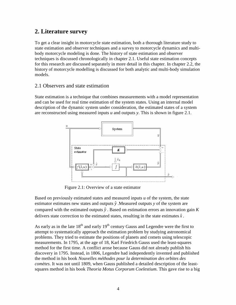
2. Literature survey To get a clear insight in motorcycle state estimation, both a thorough literature study to state estimation and observer techniques and a survey to motorcycle dynamics and multi-body motorcycle modeling is done. The history of state estimation and observer techniques is discussed chronologically in chapter 2.1. Useful state estimation concepts for this research are discussed separately in more detail in this chapter. In chapter 2.2, the history of motorcycle modelling is discussed for both analytic and multi-body simulation models. 2.1 Observers and state estimation State estimation is a technique that combines measurements with a model representation and can be used for real time estimation of the system states. Using an internal model description of the dynamic system under consideration, the estimated states of a system are reconstructed using measured inputs u and outputs y. This is shown in figure 2.1.

Figure 2.1: Overview of a state estimator

Based on previously estimated states and measured inputs u of the system, the state estimator estimates new states and outputsy .Measured outputs y of the system are compared with the estimated outputsy . Based on estimation errors an innovation gain K delivers state correction to the estimated states, resulting in the state estimatesx . As early as in the late 18th and early 19th century Gauss and Legendre were the first to attempt to systematically approach the estimation problem by studying astronomical problems. They tried to estimate the positions of planets and comets using telescopic measurements. In 1795, at the age of 18, Karl Friedrich Gauss used the least-squares method for the first time. A conflict arose because Gauss did not already publish his discovery in 1795. Instead, in 1806, Legendre had independently invented and published the method in his book Nouvelles méthodes pour la determination des orbites des comètes. It was not until 1809, when Gauss published a detailed description of the least-squares method in his book Theoria Motus Corporum Coelestium. This gave rise to a big

5

dispute between Gauss and Legendre, concerning who was the inventor of the least-squares method [10].

The next contribution in the study of the estimation problem occurred more than 100 years later, when Fisher introduced the approach of maximum likelihood estimation in 1910. In the 1940’s the next major development came with the filtering work of Wiener (1942) and Kolmogorov (1941). They both studied the problem of extracting an interesting signal in a signal-plus-noise setting and independently solved the problem, using a linear minimum mean-square technique. The solution is based on the rather restrictive assumptions of access to an infinite amount of data and that all involved signals can be described as stationary stochastic processes. During the 1940’s and 1950’s much research was directed towards extending the Wiener – Kolmogorov filtering theory.

In 1964 Luenberger showed that, for any observable linear system, an observer can be designed having the property that the estimation error can be made to go to zero as fast as one may desire [6]. The design technique is equivalent to pole placement in feedback system design. Extensions to this publication are presented in [11] and [12].

In 1961, several years before Luenberger’s introduction of observers, Kalman published his famous paper describing a recursive solution to the linear filtering problem [5]. Kalman did not longer use the conventional formulation, but the state-space theory. In 1958 Swerling already published a paper, describing a recursive procedure for orbit determination. Swerling’s method was essentially the same as Kalman’s except that the equation used to update the error covariance matrix had a slightly more cumbersome form. After Kalman had published his paper and it had attained considerable fame, Swerling wrote a letter to the AIAA Journal claiming priority for the Kalman filter equations. However, no further attention has ever been paid to this [10]. A big advantage of the Kalman filter compared with the Wiener – Kolmogorov theory is that the Kalman filter lends itself to multivariable problems, where with the Wiener – Kolmogorov theory severe problems occur when multivariable cases are considered.

The first approach to approximate a nonlinear model by a linear model was to linearize the model along a nominal trajectory, resulting in the linearized Kalman filter. Pretty soon an improvement to this was suggested by Schmidt et al [32]. They suggested that the linearization should be performed around the current estimate, rather than around a nominal trajectory. The result is the extended Kalman filter, for a detailed description see [13]. Interesting state estimation techniques for this research can be the Luenberger observer, the Kalman filter and the Extended Kalman filter because these can be applied to multivariable state estimation problems. In the next chapters it is investigated if these estimation techniques can be applied to state estimation for handling behavior. Linear observability Consider the linear dynamic system with input u, outputs y, states x and system matrices A,B,C and D:

DuCxy

BuAxx

+=+=&

(2.1)

6

If all the states of the system which are present in the state vector can be reconstructed from the sensed outputs, the system is called observable. A system which is unobservable contains states which are disconnected from the output and therefore no longer appear in the measurements [3]. This is not desirable, for no state correction can be applied anymore to the unobservable state(s).

For the linear system of (2.1) the observability matrix O can be obtained:

=

−1nCA

CA

C

OM

(2.2)

The system is observable if and only if O has full rank n, with n the dimension of the state vector. Luenberger observer If observable, a globally stable linear observer can be designed for the system of (2.1) using the pole placement technique [14]. The linear observer can be designed with the observer equations:

( )DuxCy

yyKBuxAx

+=−++=

ˆˆ

ˆˆ& (2.3)

With the error defined as xxe ˆ−= the error dynamics read:

( )eKCA

xxe

−=−=

&&& (2.4)

By choosing the values in K such that the poles of (A-KC) are located in the left halfplane, global stability is achieved.

By selecting a desired closed loop pole location for the observer an accompanying observer gain K can be calculated. The closed loop characteristic polynomial of the observer is given by: ( ) { }( )KCAI −−= λλα det (2.5) The observer gain K is found by selecting an( )λα which determines where the poles λ are to be located.

With this method only a unique solution for K is found for single-output systems. With m measurements and n states the dimensions of the system matrices are:

nxmKmxnCnxnA === , , , see (2.4). With I and A having dimensions nxn, a number of n closed loop pole locations exist for the observer in (2.3).

7

With n equations and nxm unknowns (number of gain values in K) only a unique set of observer gains exist for m=1, thus in the single-output system. In case of multi-output systems, (2.5) can also be solved but no unique solution is found. Kalman filter The problem addressed by the Kalman filter is the following. Consider the observable, linear system with input u, outputs y, states x and system matrices A,B,C and D:

vDuCxy

wBuAxx

++=++=&

(2.6)

where w and v are noise processes, having known spectral density matrices. The noises w and v are assumed to be independent of each other, white noise and with normal probability distributions with zero mean:

( )( ) ),0(~

),0(~

RNvp

QNwp (2.7)

with Q and R the process noise w covariance and measurement noise v covariance matrices respectively.

The Kalman filter is defined in state space form as in (2.3). With the error defined as xxe ˆ−= the error dynamics read:

( ) KvweKCAe −+−=& (2.8) The optimized covariance matrix P is computed via the matrix Riccati equation: QCPRPCPAAPP TT +−+= −1& (2.9) For the Kalman filter, the optimized covariance matrix P is obtained from solving the algebraic Ricatti equation for the stationary condition 0=P& . P thus is the symmetric positive definite matrix satisfying: 01 =+−+ − QCPRPCPAAP TT (2.10) From this the optimum Kalman gain matrix follows: 1−= RPCK T (2.11)

8

Non-linear state estimation, Extended Kalman filter The present TNO motorcycle state estimator is based on a non-linear Extended Kalman Filter (EKF). For a nonlinear system the nonlinear EKF equations are described by:

),ˆ(ˆ

)ˆ(),ˆ(ˆ

uxhy

yyKuxfx

=−+=&

(2.12)

With similar assumptions as with the linear Kalman Filter the optimized process noise covariance P is computed by solving the dynamic Riccati equation, see (2.9). In (2.9) the matrices A and C are the Jacobians evaluated around the current state estimate and are time varying:

)(),(ˆ)(),(ˆ

,tuutxxtuutxx x

hC

x

fA

==== ∂∂=

∂∂= (2.13)

Because the observer gain K is a result of the dynamic Riccati equation (2.9), K is a time-varying matrix.

The present TNO motorcycle state estimator design is described in [38]. This report deals with the design based on the Extended Kalman filter. Conclusions drawn here are that the Extended Kalman filter technique is effective for motorcycle state estimation, but tuning of the noise covariance matrices Q and R is a laborious task. 2.2 Motorcycle dynamics Already in the late 1860’s a lot of effort was done to analytically model the bicycle dynamics. Later on, during the 1970’s and 1980’s, this was extended to motorcycle dynamics. With the development of computers, software packages to analyze complicated multi-body motorcycle simulation models were designed. A summary of the analytic motorcycle models is given first. After this a description of the present multibody motorcycle simulation models is given. Analytic motorcycle models The history of motorcycle modelling leads back to the first attempts to describe the dynamics of a bicycle. One of the earliest attempts to analyze the dynamics of a single track vehicle is the work of Rankine in 1869. In a sequence of five short articles an inverted-pendulum-type model to study balancing, steering and propulsion is introduced [15].

The first substantial contribution to the theoretical bicycle literature however was Whipple’s seminal 1899 paper [16]. Whipple’s paper contains a set of nonlinear differential equations that describe the general motion of a bicycle and rider. Whipple used his model to analyze the stability of the bicycle. The bicycle model consists of two frames, a rear frame and a front frame, which are hinged together along an inclined steering axis, see figure 2.2. The front and the rear wheels are attached to the front and rear frames respectively, and are free to rotate relative to them. The rider is described as an inert mass that is rigidly attached to the rear frame. The rear frame is free to roll and

9

translate. There is no aerodynamic drag representation, no frame flexibility and no suspension system. The rear frame is assumed to move at a constant speed. The possibility of the rider applying a steering torque input by using a torsional steering spring is also considered. The tyres are assumed to be rigid and non-slipping in longitudinal and lateral directions.

Since appropriate computing facilities were not available at the time, Whipple’s general nonlinear equations could not be solved and consequently were not pursued beyond simply deriving and reporting them. Instead, Whipple studied a set of linear differential equations that correspond to small motions about a straight-running trim condition at a given constant speed [17]. A detailed review is given in [18]. Figure 2.2 schematically represents the Whipple bicycle.

Figure 2.2: Whipple bicycle [18]

An early attempt to introduce side-slipping and force generating tires into the bicycle literature appears in [19]. Other classical contributions to the theory of bicycle dynamics include [20] and [21].

One of the first attempts to investigate the motorcycle’s stability using a proper tyre model was made by Sharp in 1971 [7]. The model consists of two rigid bodies that are joined via a conventional steering joint and two wheels as with the Whipple bicycle. The steering freedom is constrained by a linear steering damper. The front frame consists of the front wheel, forks, handlebars and fittings. The rear frame consists of the main structure, the engine, the petrol tank, seat, rear swinging arm, the rear wheel and a rigidly attached rider. Each frame has a longitudinal plane of symmetry and the axis through the front frame mass centre parallel to the steering axis is a principal axis. The wheels are rigid discs each of which makes point contact with the road. They roll without longitudinal slip on a flat level road surface. The machine moves at a constant forward speed with freedom to side slip, yaw and roll; only small perturbations from straight running are considered. Aerodynamic side forces, yaw moments and roll moments are neglected. The tyre forces are generated by side-slip and camber angles. A representation of the Sharp 1971 model is given in figure 2.3.

10

Figure 2.3: Sharp 1971 model [25]

In the 1980’s the work of Sharp [22] and Verma [23] independently show that frame compliance should be included in the multi-body description of a motorcycle. This in order to correctly describe the eigenmodes of the motorcycle during straight running. In 1981 Spierings confirmed this in his work [24]. However, for motorcycle state estimation for handling application of modern motorcycles, frame compliance can be neglected [4]. In 1983 Koenen published his PhD work concerning a complicated motorcycle model which can be used to determine the dynamic behavior both when running straight and when cornering [8]. Especially the analysis of the dynamic behavior of the cornering motorcycle has given new insights. Koenen also used his model to report on the stability at large lateral curving accelerations which involve large roll angles and interaction of in-plane and lateral dynamics of the complex system.

In 1985 Sharp published a paper with a review of the state of knowledge and understanding of the steering behavior of single-track vehicles [25]. In this paper the model of Koenen is referred to as the most comprehensive motorcycle model. Little to no changes in motorcycle modeling can be seen until nowadays. In 2002 Pacejka made a review on the Koenen model in [9]. This model consists of 4 rigid bodies: the mainframe containing the rear wheel assembly with the engine and the rider’s legs and lower body, the front upper frame with the handlebars and the sprung parts of the front fork, the front subframe with the unsprung parts of the fork and front wheel and finally the rider’s upper torso, see figure 2.4.

Figure 2.4: Pacejka model [9]

11

The front upper frame is connected to the mainframe via a conventional steering joint along an inclined steering axis and is constrained by a viscous damping in the steering joint. The torsional flexibility of the frame is modeled by a twist axis which connects the front upper frame and the front subframe via a torsional spring with viscous damping. The rider’s upper torso is attached to the mainframe, via a torsional spring with viscous damping, and can incline along the rider lean axis. The wheels are rigid disks which makes point contact with the road. They roll without longitudinal slip on a flat level road surface. The tyre forces are generated by side-slip and camber angles using a linear tyre model. The machine moves at a constant forward speed with freedom to side slip, yaw, roll and steer. Also frame twist and rider lean are included. Only small deviations from rectilinear path are described by the model. The longitudinal tyre force and air drag can be assessed. The Pacejka analytic motorcycle model is implemented in the present TNO motorcycle state estimator, and shows a good representation of a real motorcycle. With use of some assumptions, i.e. driver roll excluded, twist degree of freedom suppressed and non-lagging behavior of the tyres, this analytic model is used for the state estimator design in this report. TNO also implemented the Pacejka model in the first version of the motorcycle state estimator, based on the Extended Kalman filter. Appendix D contains the Pacejka analytic motorcycle model differential equations. Multibody motorcycle simulation model A breakthrough in multibody motorcycle modelling came with the development of computers with more and more memory and computational capacity. This led to the development of software packages with which it is possible to analyze complicated multi-body models with relatively little effort. Recently a lot of research is conducted at the department of Mechanical Engineering of the University of Padova.

In 2000 Berritta et al presented a paper in which a multibody simulation model of a motorcycle is presented [26]. With this model the motorcycle handling is evaluated, the results obtained by simulations show very good similarity with measurements. 2 Years later Cossalter presented an improved model in [27].

In 2001 Sharp again showed confidence in the work of Koenen for a multi-body motorcycle model for computer simulations. In 2005 TNO in cooperation with the TU/e developed its own multi-body motorcycle model in Matlab SimMechanics, based on the Koenen model [28]. This motorcycle model has extensively been validated and is used for motorcycle handling simulations nowadays.

12

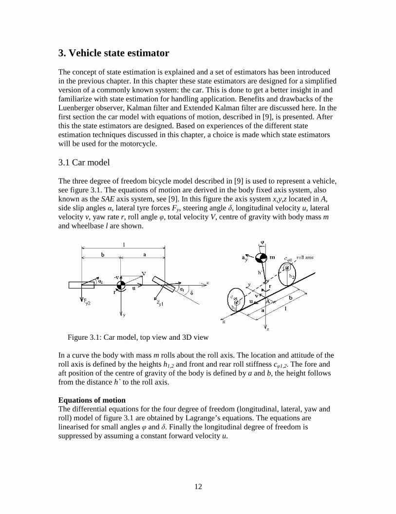
3. Vehicle state estimator The concept of state estimation is explained and a set of estimators has been introduced in the previous chapter. In this chapter these state estimators are designed for a simplified version of a commonly known system: the car. This is done to get a better insight in and familiarize with state estimation for handling application. Benefits and drawbacks of the Luenberger observer, Kalman filter and Extended Kalman filter are discussed here. In the first section the car model with equations of motion, described in [9], is presented. After this the state estimators are designed. Based on experiences of the different state estimation techniques discussed in this chapter, a choice is made which state estimators will be used for the motorcycle. 3.1 Car model The three degree of freedom bicycle model described in [9] is used to represent a vehicle, see figure 3.1. The equations of motion are derived in the body fixed axis system, also known as the SAE axis system, see [9]. In this figure the axis system x,y,z located in A, side slip angles α, lateral tyre forces Fy, steering angle δ, longitudinal velocity u, lateral velocity v, yaw rate r, roll angle φ, total velocity V, centre of gravity with body mass m and wheelbase l are shown.

Figure 3.1: Car model, top view and 3D view

In a curve the body with mass m rolls about the roll axis. The location and attitude of the roll axis is defined by the heights h1,2 and front and rear roll stiffness cφ1,2. The fore and aft position of the centre of gravity of the body is defined by a and b, the height follows from the distance h` to the roll axis. Equations of motion The differential equations for the four degree of freedom (longitudinal, lateral, yaw and roll) model of figure 3.1 are obtained by Lagrange’s equations. The equations are linearised for small angles φ and δ. Finally the longitudinal degree of freedom is suppressed by assuming a constant forward velocity u.

13

The resulting linear equations of motion for successively vy, r and φ read:

( ) 21 yyy FFhruvm +=′++ ϕ&&& (3.1)

( ) 21 yyxzzz bFaFIIrI −=−+ ϕε &&& (3.2)

( ) ( ) ( )( ) ( )ϕϕ

ϕε

ϕϕϕϕ 2121

2

cchmgBB

hmIurvhmrII xxyxzzz

−−′++−

=′+++′+−&

&&&& (3.3)

with Izz the yaw moment of inertia, Ixx roll moment of inertia, Ixz the roll/yaw product of inertia, ε the roll axis inclination angle, Bφ1 and Bφ2 the front and rear roll damping respectively, h0 the height of the roll axis below the centre of gravity and Fy1 and Fy2 the lateral forces of respectively the front and rear tyres. The differential equations describing the lateral velocity vy, the yaw rate r and the roll rateϕ& are derived from (3.1)-(3.3) and can be found in appendix A. Tyre models The lateral forces Fy1 and Fy2 are generated by the tyres. The lateral forces are functions of the respective side slip angles α1 and α2: ( )111 αyy FF = and ( )222 αyy FF = (3.4)

where for small values of α:

( )arvu y +−= 1

1 δα and ( )brvu y −−= 1

2α (3.5)

Two widely used tire models are the linear tyre model and the Magic tyre formula. For estimation an exponential tyre model is used by TNO. This model is a close representation to the Magic formula but with lower complexity. For estimation, matrices containing partial derivatives of the tyre model are required, see (2.13). For minimizing computation time, the exponential tyre model is used instead of the Magic tyre formula. The linear tyre model is given by [9]:

αα ⋅= Fy CF (3.6)

with cornering stiffness αFC .

The exponential tyre model is given as [30]:

( ) ( )αµ α signeFF Kzy ⋅−⋅= −1 (3.7)

with lateral friction coefficient µ, vertical tyre force Fz and cornering stiffness K.

14

With B, C, D and E the shape factors for the curve, the Magic tyre formula [9] is expressed as:

( ){ }[ ]ααα BBEBCDFy i arctanarctansin −−= (3.8)

Figure 3.2 shows the responses of the different tyre models.

-20 -15 -10 -5 0 5 10 15 20

-8000

-6000

-4000

-2000

0

2000

4000

6000

8000

α [deg]

Fy [

N]

Lateral force - Side slip angle

Magic Tyre Formula

Logarithmic model

Linear model

Figure 3.2: Tyre side slip characteristics

System description The tyre model of (3.8) represents the real tyre behavior closely [9]. The non-linear differential equations of motion for the system are obtained by evaluating (3.8) in the differential equations of (3.1)-(3.3). In order to put the differential equations into state space form, the state vector x and input u are defined as:

[ ] [ ]δϕϕ == urvx Ty ,& (3.9)

and with lateral acceleration ay and yaw rate r as outputs with measurement noise Vv (white noise, variances 10-2

and 10-4 respectively) the system is expressed in non-linear state space by:

[ ] ( )[ ] ( ) v

Ty

Ty

Vuxhray

uxfrvx

+==

==

,

,ϕϕ &&&&&& (3.10)

For the sake of readability of the report the complete set of equations of f(x,u) and h(x,u) are not presented here, but can be found in appendix A instead.

15

3.2 State estimator design For the system (3.11) a non-linear Extended Kalman filter is designed and two state estimators which comprise a linear approximation of the system: the linear Kalman filter and the linear Luenberger observer. For the linear state estimators, (3.10) is converted into linear state space. For the straight line driving operating condition:

[ ] [ ]0 ,0000 00 == ux T (3.11)

The linear state space matrices are obtained by:

0,0

0,0

0,0

0,0

, , ,uuxx

uuxx

uuxx

uuxx u

hDxhCu

fBxfA

==

==

==

== ∂

∂=∂∂=∂

∂=∂∂= (3.12)

The differential equations of (A.1)-(A.4) are implemented in the state estimators. The tyre model implemented in the linear state estimators is given in (3.6), the non-linear Extended Kalman filter is equipped with the tyre model of (3.7), see table 3.1. Table 3.1: System and observers, tyre models Tyre model System Non-linear, (3.8) Kalman filter Linear, (3.6) Luenberger observer Linear, (3.6) Extended Kalman filter Non-linear, (3.7) The state space equations for the Kalman filter and Luenberger observer are given by (2.3), state space equations for the Extended Kalman filter are given by (2.12). For tuning the state estimators, the performance of the state estimators is quantified by a weighted root-mean-square estimation error:

∑=

⋅=n

iii E

nE

1

1 σ (3.13)

with n the number of states, σi a weighting factor for state i and

∑=

=m

jiji xe

mE

1

2)(1

(3.14)

with estimation error ej( xi) for sample j for state i and m the number of samples.

16

Kalman filter For the observable system (3.10) a Kalman filter is designed. Two types of disturbances dominate: tyre model deviations and measurement noise. The effect of the tyre model deviations is shown in figure 3.2. The tyre model deviation results in a disturbance in both the state and output equations of the Kalman filter. The measurement noise only appears as a disturbance in the output equation. These disturbances are taken into account in the design of the Kalman filter. The design and resulting parameters for the Kalman filter are given in table 3.2. Table 3.2: Design parameters of the Kalman filter State estimator Design parameters Resulting parameters Kalman filter Q, R KKF, λKF (fixed) All modeling deviations are assumed to be a zero-mean gaussian process. Disturbances in the state equations, due to the tyre model deviations, are modeled in the process noise covariance matrix Q. Disturbances in the output equation due to the tyre model deviations together with the measurement noise are modeled in the measurement noise covariance matrix R. With Q and R, a weighting is made how state correction is applied.

The measurement noise variances of Vv are known (see section 3.1, the variances are 10-2

and 10-4 respectively). When solely dealing with measurement noise, these variances are modeled in R directly [14]. Due to the tyre model deviations, additional noise is modeled in R. The order of magnitude of this noise is not known and can not explicitly be expressed in a number. For this reason a set of R matrices is evaluated to compute the weighted RMS estimation error using (3.13). The lowest estimation error is correlated to the optimal choice of R as:

[ ]( )31 1010 −−= diagR (3.15) Consider the differential equations (A.1), (A.2), (A.3) and (A.4). The tyre model deviations appear in the lateral forces Fy1 and Fy2, thus deviations appear in the equations (A.1), (A.2) and (A.4). The tyre model deviation does not appear in (A.3). This means that error covariances in Q for the equations (A.1), (A.2) and (A.4) are higher than the error covariance for the roll motion equation (A.3). As described above the effect of the tyre model deviations can not be expressed in a number explicitly. Also Q is chosen empirically, using a set of different Q matrices and correlate the lowest estimation error (3.13) to the optimal Q, as: [ ]( )0800 10101010 −= diagQ (3.16) Note that noise covariances are assumed to be uncorrelated; Q and R are diagonal matrices.

17

The choice of Q and R results in the Kalman gain and closed loop poles:

−±−

−=

−−−

−−

=13.51

47.1497.23

11.16

,

2335.00546.0

9410.05710.0

8752.275801.0

9002.128931.2

iK KFKF λ (3.17)

Note that the Kalman gain is computed off-line by solving the stationary Ricatti equation as discussed in section 2.1. The system matrices A, B, C and D are obtained from (3.12). A Matlab implementation for the design of the Kalman filter is found in appendix C. Luenberger observer In paragraph 2.1 the Luenberger observer is introduced. The Luenberger observer is only applicable to single-output systems. Choosing only one measurement signals as output results in a stable output error dynamics LOyy ˆ− , but this does not imply a stable

observer error dynamics LOxx ˆ− for the following reason. Consider the residual:

DuxCuxhr

yyr

−−=−=

ˆ),(

ˆ (3.18)

With the system output divided in a linear part and a model mismatch error ),( uxψ due to deviations in the tyre models between system and estimators: ),(),( uxDuCxuxh ψ++= (3.19) the residual becomes:

( )),(

),(ˆ

ˆ),(

uxCer

uxxxCr

DuxCuxDuCxr

ψψψ

+=+−=

−−++= (3.20)

with state estimation error LOxxe ˆ−= . If the residual is forced to zero and the error

),( uxψ does not equal zero, the state estimation error LOxx ˆ− cannot be forced to zero.

This means that when using only yaw rate r as output, only stability of the yaw rate state is guaranteed. State estimation errors of the other states will not be forced to zero due to the model mismatch ),( uxψ . In order to minimize the weighted RMS state estimation error (3.13) it thus is necessary to consider multiple outputs. For the single-output Luenberger observer this means that outputs need to be combined to a single output.

18

For this reason the output will be modeled as:

ray y ⋅+⋅= 21 γγ (3.21)

with free to choose weighting factors γ1 and γ 2 and measurement signals ay (lateral acceleration) and r (yaw rate). In order to weight lateral acceleration and yaw rate equally the chosen output is:

ray y ⋅+⋅= 120

1 (3.22)

With this output the system is observable. Design parameters of the Luenberger observer are given in table 3.3. Table 3.3: Design parameters of the Luenberger observer State estimator Design parameters Resulting parameters Luenberger observer

λLO, γ 1, γ 2 KLO (fixed)

To be able to compare the Luenberger observer responses with those of the Kalman filter similar closed loop pole locations are taken, see (3.17). The closed loop pole locations

LOλ and Luenberger observer gain matrix KLO are:

−=

−±−

−==

5894.12

7086.99

4931.77

4152.269

,

13.53

47.1497.23

11.16

LOKFLO Kiλλ (3.23)

Appendix C contains the Matlab code for computing the Luenberger observer gain matrix KLO using desired closed loop pole locations. Extended Kalman filter Contrary to the linear Kalman filter and the Luenberger observer, the Extended Kalman filter lends itself to non-linear estimation. The design and resulting parameters of the Extended Kalman filter are given in table 3.4. Table 3.4: Design parameters of the Extended Kalman filter State estimator Design parameters Resulting parameters Extended Kalman filter

Q, R KEKF, λEKF (adaptive)

19

The Extended Kalman filter gain matrix is obtained by real-time solving the dynamic Riccati equation, see (2.9). The jacobians of f(x,u) and h(x,u) are evaluated around the current estimates, see (2.13), resulting in an adaptive observer gain matrix.

Due to computational complications when deriving the Jacobians, the exponential tyre model of (3.7) is implemented in the differential equations instead of the Magic tyre formula from (3.8). This means that the noise covariances Q and R can be modeled smaller than with the linear Kalman filter. Tyre model deviations only appear in the equations (A.1), (A.2) and (A.4). For this reason, the value in Q concerning (A.3) stays unchanged and the other values need to be decreased. As with the Kalman filter, Q can not be measured and is determined empirically as:

[ ]( )1811 10101010 −−−−= diagQ (3.24) For similar reason as explained above the noise covariances in the measurement noise covariance matrix R need to be decreased. R is determined empirically as:

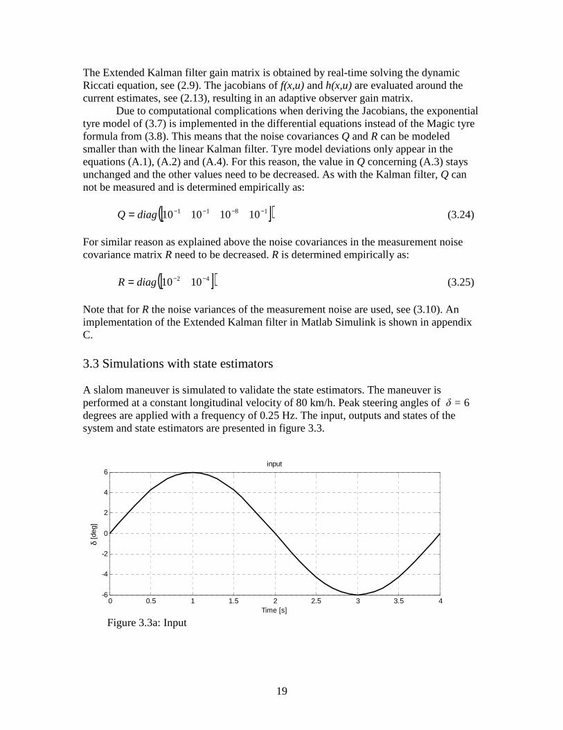
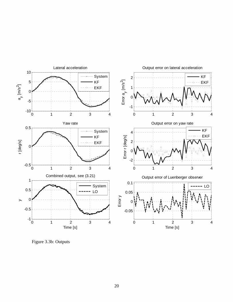
[ ]( )42 1010 −−= diagR (3.25) Note that for R the noise variances of the measurement noise are used, see (3.10). An implementation of the Extended Kalman filter in Matlab Simulink is shown in appendix C. 3.3 Simulations with state estimators A slalom maneuver is simulated to validate the state estimators. The maneuver is performed at a constant longitudinal velocity of 80 km/h. Peak steering angles of δ = 6 degrees are applied with a frequency of 0.25 Hz. The input, outputs and states of the system and state estimators are presented in figure 3.3.

0 0.5 1 1.5 2 2.5 3 3.5 4-6

-4

-2

0

2

4

6

Time [s]

δ [d

eg]

input

Figure 3.3a: Input

20

0 1 2 3 4-10

-5

0

5

10

a y [m

/s2 ]

Lateral acceleration

System

KF

EKF

0 1 2 3 4-0.5

0

0.5

r [d

eg/s

]

Yaw rate

0 1 2 3 4-1

-0.5

0

0.5

1

Time [s]

y

Combined output, see (3.21)

System

LO

0 1 2 3 4

-1

0

1

2

Err

or a

y [m

/s2 ]

Output error on lateral acceleration

KF

EKF

0 1 2 3 4

-2

0

2

4

Err

or r

[de

g/s]

Output error on yaw rate

0 1 2 3 4

-0.05

0

0.05

0.1

Time [s]

Err

or y

Output error of Luenberger observer

LO

System

KF

EKF

KF

EKF

Figure 3.3b: Outputs

21

1 2 3 4-2

0

2

v y [m

/s]

Lateral velocity

System

KF

LO

EKF

1 2 3 4

-20

0

20

r [d

eg/s

]

Yaw rate

0 1 2 3 4-20

0

20

Dφ

[deg

/s]

Time [s]

Roll rate

1 2 3 4

-5

0

5

φ [d

eg]

Roll angle

1 2 3 4

-0.5

0

0.5

Err

or v

y [m

/s]

Estimation error on lateral velocity

KF

LO

EKF

0 1 2 3 4-10

0

10

Err

or r

[de

g/s]

Estimation error on yaw rate

0 1 2 3 4-20

0

20

Err

or D

φ [d

eg/s

]

Time [s]

Estimation error on roll rate

1 2 3 4-4

-2

0

2

Err

or φ

[de

g]

Estimation error on roll angle

Figure 3.3c: States

22

The performance of the state estimators is evaluated by means of evaluating the RMS estimation errors computed with (3.14). The RMS state estimation errors for this maneuver are presented in table 3.5. Table 3.5: RMS errors for slalom maneuver KF LO EKF Evy [m/s] 0.18 0.37 0.12 Er [deg/s] 1.13 4.30 0.88 Eφ [deg/s] 0.80 1.99 0.25 Eϕ& [deg/s2] 1.77 8.82 0.82 From figure 3.3 and table 3.5 it is concluded that, due to model deviations, it is not possible to force the estimation error to zero, regardless of the stable output error dynamics. This was already explained in section 3.2. by means of (3.20).

Table 3.5 shows that the Extended Kalman filter outperforms the linear Kalman filter and Luenberger observer; the RMS errors are lowest on all states. This can be explained using figure 3.2. With a steering angle of δ = 6 degrees the system acts in a non-linear way due to the non-linear tyre behavior of the Magic tyre formula model. The exponential tyre model, implemented in the Extended Kalman filter, behaves closer to the Magic tyre formula than the linear tyre model which is implemented in both the Kalman filter and the Luenberger observer. With smaller model deviations, better performance, i.e. lower estimation errors, is obtained.

The RMS estimation errors of the Luenberger observer are significantly higher than those of the Kalman filter. This is due to the fact that the measurement signals are combined to a single output, see (3.22). By combining the measurement signals, estimation errors in the measurement signals can annihilate each other. The result of this is that LOyy ˆ− approaches zero, while LOxx ˆ− does not. With a different choice for the

weighting factors γ 1 and γ 2 and different closed loop poles (3.23), different responses are obtained. Choosing either γ1 or γ 2 equal to zero however is not a solution, this was explained in section 3.2. Perhaps a better tuning is possible using different weighting factors of closed loop observer pole locations. However, there is neither a structured method to design γ 1 and γ 2 nor to choose closed loop observer pole locations. For this reason the pole placement technique is not used in the rest of this research. A different method for tuning a linear observer is proposed in the next chapter.

From the results above it can be concluded that the linear Kalman filter behaves robust for the significant non-linearity’s introduced here. Tuning of the Kalman filter is not straightforward and demands knowledge of the system, noise covariances need to be determined empirically. However, the possibility to apply the Kalman filter to multi-output systems, combined with the possibility to perform linear simulations fast, are of such benefits that the Kalman filter (and a variant of the linear observer) are used for the final design of the motorcycle state estimator.

23

3.4 Summary The Extended Kalman filter, linear Kalman filter and Luenberger observer have been designed and tuned for a passenger car. The state estimators are validated for car handling behavior. The proposed Extended and linear Kalman filter perform as desired. However the design parameters, the noise covariance matrices Q and R, can not be measured but need to be tuned empirically. The Luenberger observer in the form used in this chapter is not applicable to multi-output state estimation and will not be used for further investigation. For motorcycle state estimation both the Extended Kalman filter and linear Kalman filter are advised.

24

4. Optimized linear observer In the next chapters linear motorcycle state estimators are designed and validated for a simulation motorcycle model and for a real motorcycle. In the previous chapter it was shown that the linear Kalman filter can be used for state estimation applied to handling application. This chapter describes the design of a new type of linear observer which can also be used for motorcycle state estimation the optimized linear observer. 4.1 Motivation and difference to conventional method Tuning of the TNO motorcycle state estimator based on the Extended Kalman filter is found to be a laborious task, demanding large computational effort and manual intervention [4]. Two problems for tuning the TNO motorcycle state estimator dominate. First, knowledge of deviations between the analytic model, implemented in the filter, and reality is required to define the noise covariance matrices Q and R, secondly due to the non-linear equations, simulations are performed relatively slow, in the order of real-time (on a 2Ghz PC). When assuming linear behavior of the system, a linear Kalman filter can be designed for the estimation task. A major advantage of this is that, when using a linear state estimator, linear simulations can be done which are performed in the order of 1000 times real-time. Still, knowledge about deviations of the analytic model from reality needs to be known to define the noise covariance matrices Q and R. When using linear simulations this is less of an issue because the low simulation times allow for determining Q and R empirically.

Due to the presence of model deviations and measurement noise it is not possible to force the estimation error xx ˆ− to zero. With the Kalman filter, model error noise with variance w and measurement noise with variance v are modeled in respectively the process noise covariance matrix Q and measurement noise covariance matrix R. By tuning Q and R the covariance matrix P and innovation gain matrix K are optimized, resulting in a minimized estimation error, see (2.10). Due to symmetry of Q and R, with a number of n states and m outputs the number of design parameters for Q and R

respectively is ( )2

2 nn + and ( )2

2 mm + .

Because of the large number of design parameters for large systems, tuning Q and R is a laborious task, even with linear simulations. For this reason it often is assumed that noise covariances are not cross correlated, resulting in a reduction of the design parameters for Q and R to n and m respectively. For many real-life systems this assumption however is not correct and the optimal innovation gain matrix K resulting in an as low as possible estimation error is not found. Also Kalman filtering assumes that the process and measurement noise are white noise and with normal probability distributions with zero mean, see section 2.1. Based on these assumptions Q and R are modeled and via the Riccati equation the optimal innovation gain matrix K is found. For some systems the assumptions concerning the noises w and v can be incorrect, for instance when dealing with a systematic error. This means, again, that the innovation gain matrix K which results in an as low as possible estimation error, is not found.

25

For obtaining the optimal innovation gain for the Kalman filter, it is thus necessary to design Q and R matrices which also contain off-diagonal elements. This means that

tuning the symmetric Q and R matrix results in a total of ( ) ( )2

22 mmnn +++ design

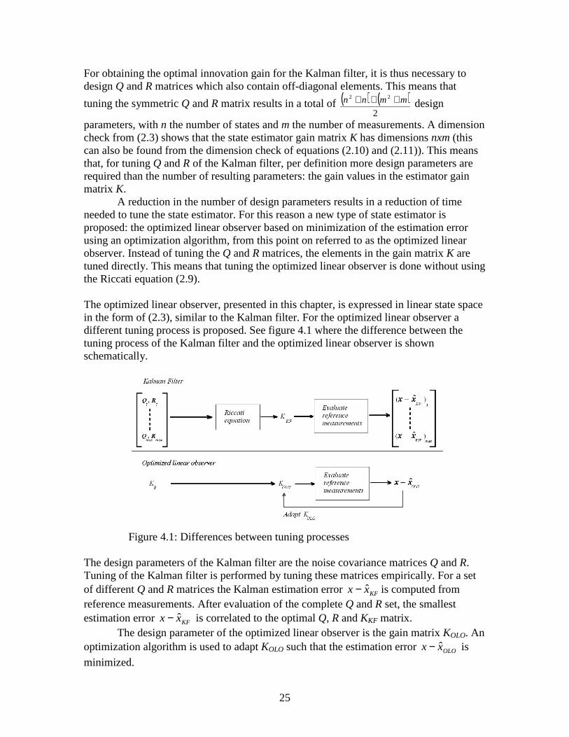
parameters, with n the number of states and m the number of measurements. A dimension check from (2.3) shows that the state estimator gain matrix K has dimensions nxm (this can also be found from the dimension check of equations (2.10) and (2.11)). This means that, for tuning Q and R of the Kalman filter, per definition more design parameters are required than the number of resulting parameters: the gain values in the estimator gain matrix K. A reduction in the number of design parameters results in a reduction of time needed to tune the state estimator. For this reason a new type of state estimator is proposed: the optimized linear observer based on minimization of the estimation error using an optimization algorithm, from this point on referred to as the optimized linear observer. Instead of tuning the Q and R matrices, the elements in the gain matrix K are tuned directly. This means that tuning the optimized linear observer is done without using the Riccati equation (2.9). The optimized linear observer, presented in this chapter, is expressed in linear state space in the form of (2.3), similar to the Kalman filter. For the optimized linear observer a different tuning process is proposed. See figure 4.1 where the difference between the tuning process of the Kalman filter and the optimized linear observer is shown schematically.

Figure 4.1: Differences between tuning processes

The design parameters of the Kalman filter are the noise covariance matrices Q and R. Tuning of the Kalman filter is performed by tuning these matrices empirically. For a set of different Q and R matrices the Kalman estimation error KFxx ˆ− is computed from reference measurements. After evaluation of the complete Q and R set, the smallest estimation error KFxx ˆ− is correlated to the optimal Q, R and KKF matrix. The design parameter of the optimized linear observer is the gain matrix KOLO. An optimization algorithm is used to adapt KOLO such that the estimation error OLOxx ˆ− is

minimized.

26

Note that there is an important difference between the tuning of the Kalman filter and tuning of the optimized linear observer. The Kalman filter is tuned empirically, the optimized linear observer is tuned using an optimization algorithm. Tuning of the Kalman filter can also be done using the optimization algorithm, but this is not performed due the non-convexity of the tuning problem and tuning the Kalman filter emperically is performed faster than using an optimization routine. This will be explained later on in more detail. Note that tuning the Kalman filter can deliver a totally different gain matrix than obtained from the tuning method of the optimized linear observer. 4.2 Optimization algorithm The optimization algorithm is an algorithm to minimize an objective function. With k an element of the gain matrix KOLO, f(k) the objective function to be minimized, n the number of states and iσ a weighting factor on state i, the optimization problem is

expressed with the objective function:

∑=

⋅=n

iii

kE

nkf

1

1)( minimize σ (4.1)

with the root-mean-square state estimation error for state i:

∑=

=m

jiji xe

mE

1

2)(1

(4.2)

and with state estimation error ej( xi) for sample j and m the number of time samples from the reference measurement.:

( ) OLOiiij xxxe ˆ−= (4.3)

The optimization problem is solved by making bounded perturbations in the gain matrix KOLO. With the weighting factor an indication is given to what extend an estimation error on the state under consideration is undesired and needs to be minimized. A large weighting factor, relative to the other weighting factors, results in a tuning which minimizes the estimation error on the state under consideration. To prevent an unstable behavior, the optimization problem is subjected to constraints concerning closed loop state estimator pole locations obtained from: ( )CKAeig OLOOLO ⋅−=λ (4.4)

The (in)equality constraint is defined as: ( ) 0<OLOreal λ (4.5)

27

Infinitely high gain values are not desired because this on one hand results in too large computation times without gaining in accuracy or robustness and on the other hand in infinitely high noise amplification. In order to prevent the optimization algorithm to produce undesirable results, even when the constraint (4.5) is met, lower and upper bounds to the parameters in the gain matrix KOLO are defined. The bounds are determined empirically. Simulations show that with the bounds (4.6) good performance is obtained. Defining higher bounds does not noticeably result in an increase of performance. The bounds used in this research are:

200200 ≤≤− k (4.6) The Kalman gain KKF is chosen as starting gain matrix K0 for the optimization process: KFKK =0 (4.7)

A schematic overview of the tuning process is given in figure 4.2.

Figure 4.2: Optimization algorithm The optimization process starts with an initial gain matrix K0. The state estimates are obtained from reference measurements and a weighted estimation error EOLO is computed. A check is done if certain tolerances are met and the optimization process can be stopped. Based on results of the previous iteration (EOLO) -1 the optimization algorithm determines a new gain matrix KOLO with which the estimation error will be lowered for the same set of reference measurements. If predefined constraints are met the new gain matrix is used as input for the next iteration of the optimization process. This process is repeated until the stopping criterion is met. The design parameters for the optimized linear observer read: Table 4.1: Design parameters of the optimized linear observer Objective function f(k), (4.3) Constraints λOLO, (4.5) Constraints / Boundaries maxmin ≤≤ k , (4.6) Starting point K0 = KKF, (4.7) Stopping criterion Tolerances to f(k), Hessian of f(k),

boundaries of k Reference measurements Representative for the complete operating

range of the system under consideration

28

4.3 Matlab implementation The power of the tuning process of the optimized linear observer lies in the linear simulations which are performed fast, combined with the numerical optimization algorithm. The tuning process comprises two important algorithms: - fmincon.m: Non-linear constrained optimization; the optimization algorithm - lsim.m: Linear simulations of LTI state space models with which the objective function is evaluated Based on the behavior of the objective function, the weighted RMS prediction error from (4.3), the fmincon algorithm determines a gain matrix KOLO. The objective function is computed from the measured reference x and the optimized linear observer responsesOLOx , see (4.1). The optimized linear observer responses OLOx follow from the

lsim algorithm. The lsim command requires a linear system and performs simulations of LTI models in the state space representation:

DuCxy

BuAxx

+=+=&

(4.8)

The observer equations are expressed by:

( )

DuxCy

yyKBuxAx

+=−++=

ˆˆ

ˆˆ& (4.9)

Equation (4.9) has to be converted to the form of (4.8) to be able to use the lsim command. Equation (4.9) is rewritten to:

( )

DuxCy

DuxCyKBuxAx

+=−−++=

ˆˆ

ˆˆ& (4.10)

Which equals:

( ) ( )

DuxCy

KyuKDBxKCAx

+=+−+−=

ˆˆ

ˆ& (4.11)

This is converted into the standard state space representation of (4.8) by including the measurements y to the input. With:

=

y

uu* (4.12)

29

equation (4.11) becomes:

( ) [ ]

[ ] *

*

0ˆˆ

ˆˆ

uDxCy

uKKDBxKCAx

+=−+−=&

(4.13)

The fmincon algorithms uses two algorithms of a lower level; one to calculate the objective function and one to check if constraints are met. The objective function is implemented in the file obj_func.m, the constraints are implemented in the file constraint_func.m. The fmincon algorithm is called by the command: [k_opt, error] = fmincon(‘obj_func’,K0,[],[],[],[], LB,UB,’constraint_func’,options) K_OLO = reshape(k_opt,4,3) This returns the optimized linear observer gain matrix KOLO and the final value of the objective function error determined from (4.1). K0 and LB and UB are defined in equations (4.7) and (4.6) respectively. In options the stopping criterion is defined. 4.4 Summary A new type of linear observer is introduced in this chapter: the optimized linear observer. Using an optimization algorithm, the gain matrix of the optimized linear observer is found. The optimization problem addressed here is to minimize a weighted state estimation error making bounded perturbations in the gain matrix. Bounds and constraints to the gain matrix prevent the optimization algorithm to produce undesirable results. The optimized linear observer is applied to motorcycle state estimation for handling application in chapters 5 and 6 for a simulation motorcycle model and a real motorcycle respectively.

30

5. State estimator design for a virtual motorcycle The final goal of this research is to design a robust motorcycle state estimator which is easy to tune and can be applied to state estimation of a real motorcycle. Before designing a state estimator for a real motorcycle, first a state estimator is designed for a simulation model of a motorcycle: the virtual motorcycle. First this is done to get familiar with state estimation for unstable systems and second with a simulation model the motorcycle dynamics can be excluded from external disturbances like sensor noise. Without the presence of disturbances a check can be made if the motorcycle dynamics are captured properly by the analytic model implemented in the state estimator (see section 2.1). Because the simulation model is an accurate representation of a real motorcycle, conclusions drawn here can be applied to the design of a real motorcycle state estimator at a later stage. In this study 3 different types of motorcycles are used; the real motorcycle, virtual motorcycle and estimator motorcycle. For complexity reasons the motorcycle models differ in many ways.

Figure 5.1: Complexity of motorcycle This chapter focuses on the design of a motorcycle state estimator, based on the estimator motorcycle, applied to motorcycle state estimation of the virtual motorcycle simulation model. Chapter six focuses on the design of a motorcycle state estimator applied to the real motorcycle. For the estimator motorcycle the Pacejka model is used, see section 2.2. Differences between the virtual motorcycle and Pacejka model are presented in table 5.1.

31

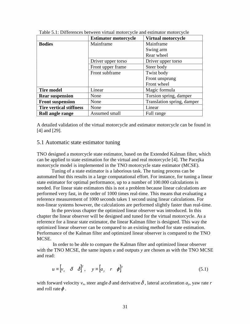
Table 5.1: Differences between virtual motorcycle and estimator motorcycle Estimator motorcycle Virtual motorcycle

Mainframe Mainframe Swing arm Rear wheel

Driver upper torso Driver upper torso Front upper frame Steer body

Bodies

Front subframe Twist body Front unsprung Front wheel

Tire model Linear Magic formula Rear suspension None Torsion spring, damper Front suspension None Translation spring, damper Tire vertical stiffness None Linear Roll angle range Assumed small Full range

A detailed validation of the virtual motorcycle and estimator motorcycle can be found in [4] and [29]. 5.1 Automatic state estimator tuning TNO designed a motorcycle state estimator, based on the Extended Kalman filter, which can be applied to state estimation for the virtual and real motorcycle [4]. The Pacejka motorcycle model is implemented in the TNO motorcycle state estimator (MCSE).

Tuning of a state estimator is a laborious task. The tuning process can be automated but this results in a large computational effort. For instance, for tuning a linear state estimator for optimal performance, up to a number of 100.000 calculations is needed. For linear state estimators this is not a problem because linear calculations are performed very fast, in the order of 1000 times real-time. This means that evaluating a reference measurement of 1000 seconds takes 1 second using linear calculations. For non-linear systems however, the calculations are performed slightly faster than real-time.

In the previous chapter the optimized linear observer was introduced. In this chapter the linear observer will be designed and tuned for the virtual motorcycle. As a reference for a linear state estimator, the linear Kalman filter is designed. This way the optimized linear observer can be compared to an existing method for state estimation. Performance of the Kalman filter and optimized linear observer is compared to the TNO MCSE.

In order to be able to compare the Kalman filter and optimized linear observer with the TNO MCSE, the same inputs u and outputs y are chosen as with the TNO MCSE and read:

[ ] [ ]Ty

T

x rayvu ϕδδ && == , (5.1)

with forward velocity vx, steer angleδ and derivativeδ& , lateral acceleration ay, yaw rate r and roll rateϕ& .

32

With the state estimator state space equations as in (2.3) the states are:

[ ]Ty rvx ϕϕ &= (5.2)

The state space matrices A,B,C and D for both the Kalman filter and optimized linear observer are obtained by linearizing the Pacejka motorcycle model for straight line driving with a constant forward velocity of vx = 72 km/h (20 m/s). When deriving the differential equations Pacejka considered only small roll motions [1]. It thus is of no use to determine the state space matrices for operating points other than straight line driving. The forward velocity of 72 km/h is chosen arbitrarily; the goal of this chapter is to get familiar with state estimation for unstable systems, not to design a state estimator which captures the complete driving range. In fact, the motorcycle simulation model lacks a driver model and no limit handling maneuvers can be simulated.

Tuning of both state estimators is performed automatically, using reference measurements x obtained from the virtual motorcycle simulation model, see figure 5.2.

Figure 5.2: Tuning of state estimators

Inputs of the tuning process are the simulation inputs u and the state estimator gain matrix K. The output E is computed from the reference measurements x and the state estimatesx and reads:

∑=

⋅=n

iii E

nE

1

1 σ (5.3)

with n the number of states, iσ a weighting factor on state i and Ei as defined in (4.2).

The input u is used to define maneuvers; dynamic slaloms and steady state cornering maneuvers. Tuning is performed by evaluating a number of gain matrices K with fixed input u. Evaluation of the outputs E result in the desired gain matrix K. Tuning the Kalman filter is done empirically, tuning the optimized linear observer is done using the optimization algorithm. In the next sections this is explained in more detail.

33

Kalman filter For the non-linear system, the virtual motorcycle, a Kalman filter is designed. The Kalman filter is expressed in state space form (2.3). In this, input u is as in (5.1) and statesxand outputsy are the estimates of x and y as in equations (5.1) and (5.2) respectively. As described above, the state space matrices A,B,C and D are obtained by linearizing the Pacejka motorcycle model for straight line driving with a forward velocity of 72 km/h (20 m/s). Table 5.2 presents the design parameters of the Kalman filter. Table 5.2: Design parameters of the Kalman filter State estimator Design parameters Resulting parameters Kalman filter Q, R KKF, λKF System and measurement noises are modeled in respectively the process noise covariance matrix Q and measurement noise covariance matrix R. Modeling small covariances in Q results in small innovation terms, modeling small covariances in R result in large innovation terms, see also (2.10) and (2.11). With the noise covariance matrices thus a weighting can be made how the state innovation is applied. As discussed earlier the measurement noise covariances can be measured and designed in R directly. The system noise covariances however can not be measured and need to be determined empirically.

Due to simplifications to the model there are model mismatches; deviations between the model and reality. In the previous chapters, model mismatches were assumed to be zero-mean gaussian processes. This assumption allowed for accounting the mismatches in Q and R by increasing the noise covariances. In reality however, model mismatches can not be represented by zero-mean guassian processes with fixed variances. However, it is possible to inject uncertainty into the noise covariance matrices Q and R, resulting in an adapted state innovation. This way model mismatches are not compensated for, but are taken into account.

This means that in Q model deviations in the differential state equations are accounted for and in R the model deviations in the output equations plus measurement noise. Note that with the simulation model measurement noise is excluded and thus only model deviations in the output equations are modeled in R. Two model differences dominate between the virtual motorcycle and the Pacejka analytic motorcycle model; a tyre model difference and a difference between roll angle range, see table 5.1. The model differences are found in both the state and output equations of the Kalman filter, equations (5.1) and (5.2) respectively. For the state differential equations the model differences only appear in the equations for ϕ&&&& and , rvy , not in the equation

forϕ& , see (A.3). This means that process noise covariances for the ϕ&&&& and , rvy equations

are higher than the noise covariance for theϕ& equation. The effect of the model errors can not be measured, Q0 is determined empirically: [ ]( )0800

0 10101010 −= diagQ (5.4)

34

For the output equations the model mismatches are only found in the lateral acceleration ay equation, not in the yaw rate r or roll rateϕ& equation. The yaw rate only contains a small orientation error due to linearization for small roll angles. No additional measurement noise is added, R0 is determined empirically and reads: [ ]( )320

0 101010 −−= diagR (5.5)

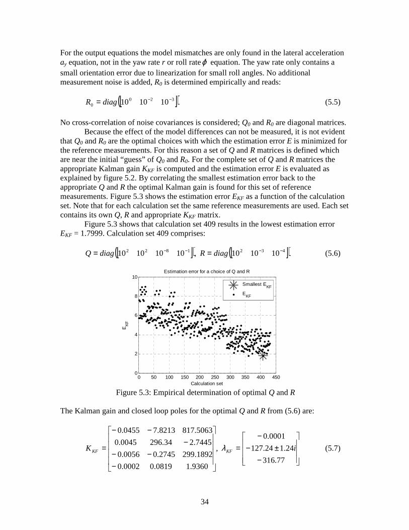
No cross-correlation of noise covariances is considered; Q0 and R0 are diagonal matrices. Because the effect of the model differences can not be measured, it is not evident

that Q0 and R0 are the optimal choices with which the estimation error E is minimized for the reference measurements. For this reason a set of Q and R matrices is defined which are near the initial “guess” of Q0 and R0. For the complete set of Q and R matrices the appropriate Kalman gain KKF is computed and the estimation error E is evaluated as explained by figure 5.2. By correlating the smallest estimation error back to the appropriate Q and R the optimal Kalman gain is found for this set of reference measurements. Figure 5.3 shows the estimation error EKF as a function of the calculation set. Note that for each calculation set the same reference measurements are used. Each set contains its own Q, R and appropriate KKF matrix.

Figure 5.3 shows that calculation set 409 results in the lowest estimation error EKF = 1.7999. Calculation set 409 comprises: [ ]( ) [ ]( )4321822 101010 ,10101010 −−−− == diagRdiagQ (5.6)

0 50 100 150 200 250 300 350 400 450

0

2

4

6

8

10Estimation error for a choice of Q and R

Calculation set

EK

F

Smallest EKF

EKF

Figure 5.3: Empirical determination of optimal Q and R

The Kalman gain and closed loop poles for the optimal Q and R from (5.6) are:

−±−

−=

−−−

−−−

=77.316

24.124.127

0001.0

,

9360.10819.00002.0

1892.2992745.00056.0

7445.234.2960045.0

5063.8178213.70455.0

iK KFKF λ (5.7)

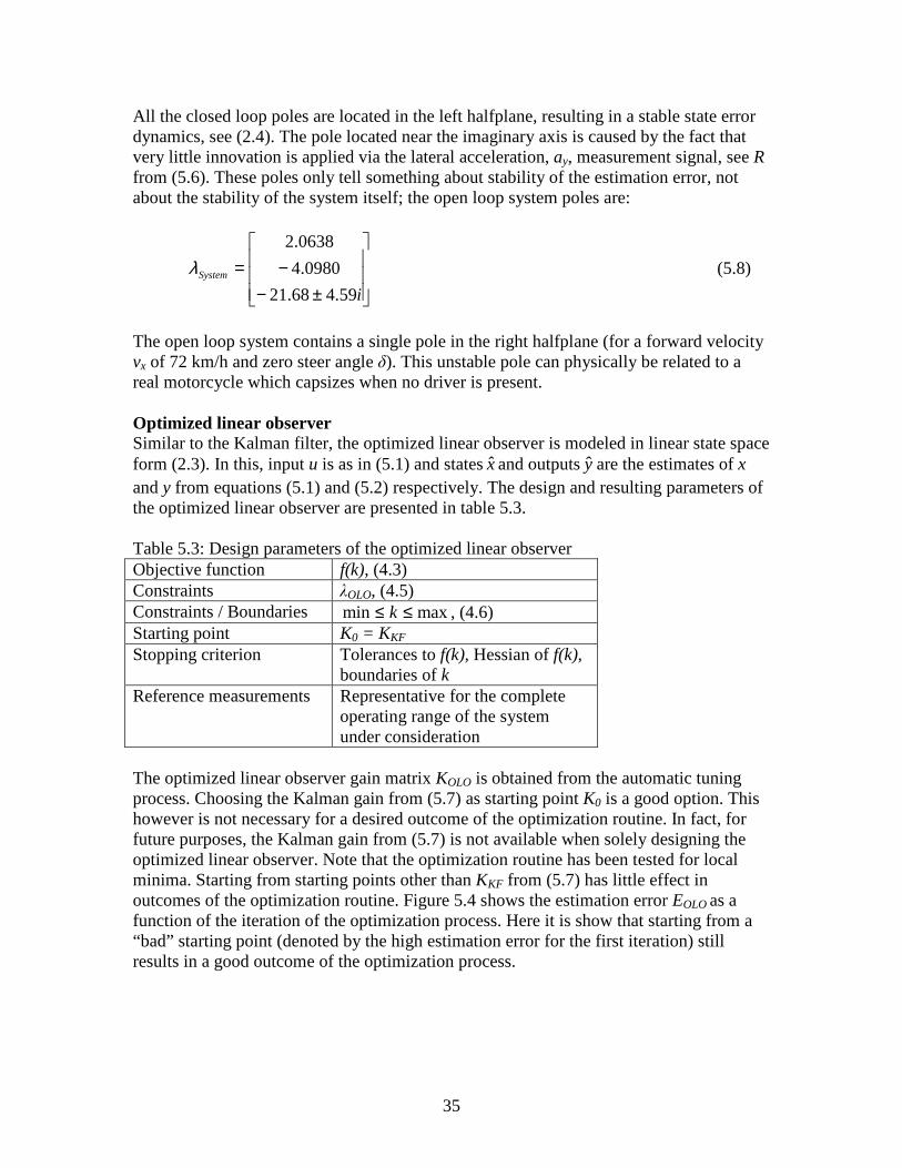
35

All the closed loop poles are located in the left halfplane, resulting in a stable state error dynamics, see (2.4). The pole located near the imaginary axis is caused by the fact that very little innovation is applied via the lateral acceleration, ay, measurement signal, see R from (5.6). These poles only tell something about stability of the estimation error, not about the stability of the system itself; the open loop system poles are:

±−−=

iSystem

59.468.21

0980.4

0638.2

λ (5.8)

The open loop system contains a single pole in the right halfplane (for a forward velocity vx of 72 km/h and zero steer angle δ). This unstable pole can physically be related to a real motorcycle which capsizes when no driver is present. Optimized linear observer Similar to the Kalman filter, the optimized linear observer is modeled in linear state space form (2.3). In this, input u is as in (5.1) and statesxand outputsy are the estimates of x and y from equations (5.1) and (5.2) respectively. The design and resulting parameters of the optimized linear observer are presented in table 5.3. Table 5.3: Design parameters of the optimized linear observer Objective function f(k), (4.3) Constraints λOLO, (4.5) Constraints / Boundaries maxmin ≤≤ k , (4.6) Starting point K0 = KKF Stopping criterion Tolerances to f(k), Hessian of f(k),

boundaries of k Reference measurements Representative for the complete

operating range of the system under consideration

The optimized linear observer gain matrix KOLO is obtained from the automatic tuning process. Choosing the Kalman gain from (5.7) as starting point K0 is a good option. This however is not necessary for a desired outcome of the optimization routine. In fact, for future purposes, the Kalman gain from (5.7) is not available when solely designing the optimized linear observer. Note that the optimization routine has been tested for local minima. Starting from starting points other than KKF from (5.7) has little effect in outcomes of the optimization routine. Figure 5.4 shows the estimation error EOLO as a function of the iteration of the optimization process. Here it is show that starting from a “bad” starting point (denoted by the high estimation error for the first iteration) still results in a good outcome of the optimization process.

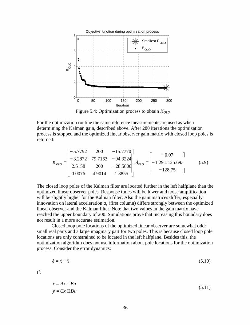
36

0 50 100 150 200 250 3000

2

4

6

8

Iteration

EO

LO

Objective function during optimization process

Smallest EOLO

EOLO

Figure 5.4: Optimization process to obtain KOLO

For the optimization routine the same reference measurements are used as when determining the Kalman gain, described above. After 280 iterations the optimization process is stopped and the optimized linear observer gain matrix with closed loop poles is returned:

−±−

−=

−−−−−

=75.128

69.12529.1

07.0

,

3855.19014.40076.0

5800.282005158.2

3224.947163.792872.3

7770.152007792.5

iK OLOOLO λ (5.9)

The closed loop poles of the Kalman filter are located further in the left halfplane than the optimized linear observer poles. Response times will be lower and noise amplification will be slightly higher for the Kalman filter. Also the gain matrices differ; especially innovation on lateral acceleration ay (first column) differs strongly between the optimized linear observer and the Kalman filter. Note that two values in the gain matrix have reached the upper boundary of 200. Simulations prove that increasing this boundary does not result in a more accurate estimation.

Closed loop pole locations of the optimized linear observer are somewhat odd: small real parts and a large imaginary part for two poles. This is because closed loop pole locations are only constrained to be located in the left halfplane. Besides this, the optimization algorithm does not use information about pole locations for the optimization process. Consider the error dynamics:

xxe &&& ˆ−= (5.10) If:

DuCxy

BuAxx

+=+=&

(5.11)

37

holds for the virtual motorcycle andx& andy are obtained from (2.3), then the error dynamics are described by: ( )eKCAe −=& (5.12) with estimation error xxe ˆ−= , and closed loop poles in the left halfplane will imply stability of the error dynamics. However, if (5.11) is disturbed by model deviations, (5.12) will no longer describe the error dynamics exactly and closed loop pole locations, which are determined from A-KC, are not an exact measure for the behavior of the error dynamics. 5.2 Simulations with virtual motorcycle state estimators The virtual motorcycle simulation model is not equipped with a driver model. For this reason no desired path can be described and simulated. However, limited measurement data from the real motorcycle can be used for a replay of the maneuver with the virtual motorcycle. Data from severe driving maneuvers can not be used for a replay. To validate the Kalman filter and the optimized linear observer a steady state cornering maneuver is simulated. The maneuver is performed at a longitudinal velocity of vx = 72 km/h. The peak roll angle φ during this maneuver approximates 40 degrees, in this region the virtual motorcycle behaves non-linear. Performance of the state estimators is tested by means of evaluating the RMS state prediction error of (4.2). Inputs, outputs and states of the system and state estimators for the steady state cornering maneuver are presented in figure 5.5.

0 10 20 30 40 50 60 7015

20

25Forward velocity

v x [m

/s]

0 10 20 30 40 50 60 70-5

0

5

Dδ

[deg

/s]

Time [s]

Steer rate0 10 20 30 40 50 60 70

-2

0

2

δ [d

eg]

Steer angle

Figure 5.5a: Inputs

38

10 20 30 40 50 60 70

-2

0

2

a y [m

/s2 ]

Lateral acceleration

System

KF

OLO

TNO MCSE

10 20 30 40 50 60

-1

0

1

2

Err

or a

y [m

/s2 ]

Output error on lateral acceleration

KF

OLO

TNO MCSE

10 20 30 40 50 60

-20

-10

0

r [d

eg/s

]

Yaw rate

10 20 30 40 50 60

-4

-2

0

2

4E

rror

r [

deg/

s]

Output error on yaw rate

10 20 30 40 50 60

-20

-10

0

10

20

Dφ

[deg

/s]

Time [s]

Roll rate

10 20 30 40 50 60

-20

-10

0

10

20

Err

or D

φ [d

eg/s

]

Time [s]

Output error on roll rate

Figure 5.5b: Outputs

39

0 10 20 30 40 50 60 70-0.4

-0.2

0

0.2

0.4

v y [m

/s]

Lateral velocity

System

KF

OLO

TNO MCSE

10 20 30 40 50 60

0

0.2

0.4

Err

or v

y [m

/s]

Estimation error on lateral velocity

KF

OLO

TNO MCSE

10 20 30 40 50 60

-20

-10

0

r [d

eg/s

]

Yaw rate

10 20 30 40 50 60-4

-2

0

2

4

Err

or r

[de

g/s]

Estimation error on yaw rate

10 20 30 40 50 60

-20

0

20

Dφ

[deg

/s]

Time [s]

Roll rate

10 20 30 40 50 60-20

-10

0

10

Err

or D

φ [d

eg/s

]

Time [s]

Estimation error on roll rate

10 20 30 40 50 60

10

20

30

40

φ [d

eg]

Roll angle

10 20 30 40 50 60

-4

-2

0

2

Err

or φ

[de

g]

Estimation error on roll angle

Figure 5.5c: States

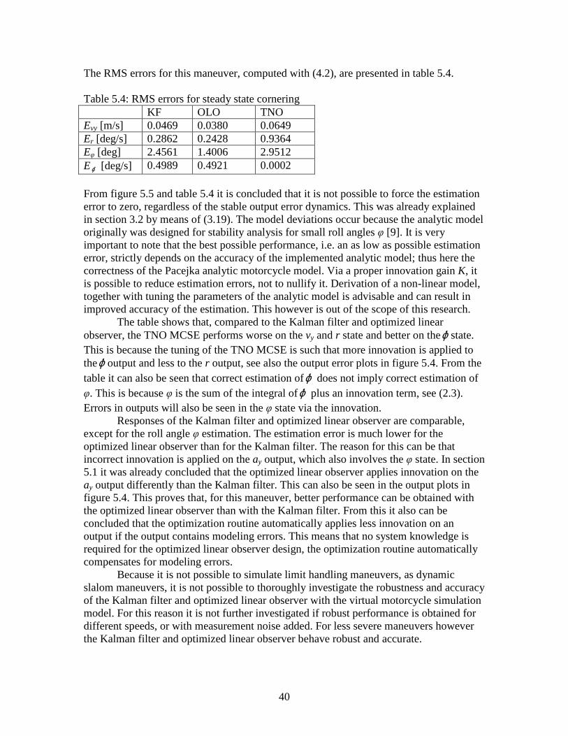
40

The RMS errors for this maneuver, computed with (4.2), are presented in table 5.4. Table 5.4: RMS errors for steady state cornering KF OLO TNO Evy [m/s] 0.0469 0.0380 0.0649 Er [deg/s] 0.2862 0.2428 0.9364 Eφ [deg] 2.4561 1.4006 2.9512 Eϕ& [deg/s] 0.4989 0.4921 0.0002 From figure 5.5 and table 5.4 it is concluded that it is not possible to force the estimation error to zero, regardless of the stable output error dynamics. This was already explained in section 3.2 by means of (3.19). The model deviations occur because the analytic model originally was designed for stability analysis for small roll angles φ [9]. It is very important to note that the best possible performance, i.e. an as low as possible estimation error, strictly depends on the accuracy of the implemented analytic model; thus here the correctness of the Pacejka analytic motorcycle model. Via a proper innovation gain K, it is possible to reduce estimation errors, not to nullify it. Derivation of a non-linear model, together with tuning the parameters of the analytic model is advisable and can result in improved accuracy of the estimation. This however is out of the scope of this research. The table shows that, compared to the Kalman filter and optimized linear observer, the TNO MCSE performs worse on the vy and r state and better on theϕ& state. This is because the tuning of the TNO MCSE is such that more innovation is applied to theϕ& output and less to the r output, see also the output error plots in figure 5.4. From the table it can also be seen that correct estimation of ϕ& does not imply correct estimation of φ. This is because φ is the sum of the integral ofϕ& plus an innovation term, see (2.3). Errors in outputs will also be seen in the φ state via the innovation.

Responses of the Kalman filter and optimized linear observer are comparable, except for the roll angle φ estimation. The estimation error is much lower for the optimized linear observer than for the Kalman filter. The reason for this can be that incorrect innovation is applied on the ay output, which also involves the φ state. In section 5.1 it was already concluded that the optimized linear observer applies innovation on the ay output differently than the Kalman filter. This can also be seen in the output plots in figure 5.4. This proves that, for this maneuver, better performance can be obtained with the optimized linear observer than with the Kalman filter. From this it also can be concluded that the optimization routine automatically applies less innovation on an output if the output contains modeling errors. This means that no system knowledge is required for the optimized linear observer design, the optimization routine automatically compensates for modeling errors.

Because it is not possible to simulate limit handling maneuvers, as dynamic slalom maneuvers, it is not possible to thoroughly investigate the robustness and accuracy of the Kalman filter and optimized linear observer with the virtual motorcycle simulation model. For this reason it is not further investigated if robust performance is obtained for different speeds, or with measurement noise added. For less severe maneuvers however the Kalman filter and optimized linear observer behave robust and accurate.

41

5.3 Summary The automatic state estimator tuning process delivers gain matrices KKF and KOLO for both the Kalman filter and optimized linear observer respectively. Simulations show that good performance is obtained from both the filter and the observer. Due to deviations in the Pacejka analytic motorcycle model it is not possible to force estimation errors to zero. Derivation of a non-linear model, together with tuning the parameters of the analytic model is advisable and can result in more accurate state estimation. For the maneuvers simulated in this chapter, with the optimized linear observer slightly better results are obtained than with the Kalman filter and the TNO motorcycle state estimator. Differences between state estimation errors occur due to different philosophies and methods used when tuning the state estimators. Overall no large differences exist between the state estimators performance.

Because of the lack of a driver model, no limit handling maneuvers can be simulated and no judgments are done concerning accuracy and robustness of the state estimators for more severe maneuvers. For this reason no further investigation is done with the virtual motorcycle simulation model.

42

6. State estimator design for a real motorcycle Two linear state estimators are designed for the virtual motorcycle simulation model in the previous chapter. Results from simulations learned that the linear Kalman filter and optimized linear observer can be used for motorcycle state estimation for handling behavior. This chapter is conducted to the state estimator design for a real motorcycle. The estimator motorcycle, implemented in both state estimators, is the Pacejka analytic motorcycle model, the similar as used in the previous chapter. The reference state estimator is the TNO Motorcycle State Estimator, based on the Extended Kalman filter.

Compared to the virtual motorcycle, the real motorcycle is more complex, see figure 5.1. The differences between the estimator and real motorcycle are presented in table 6.1. Comparing table 6.1 with table 5.1 shows that the real motorcycle comprises more bodies and tyre behavior is different from the virtual motorcycle. This means that deviations between the estimator motorcycle and real motorcycle can be larger than deviations between the estimator motorcycle and virtual motorcycle.

Table 6.1: Differences between motorcycles Estimator

motorcycle Real motorcycle

Mainframe Mainframe, engine, mirrors, rear wheel, exhaust, tail light

Driver upper torso Driver upper torso, helmet Front upper frame Frame caster, sprung front fork, headlight,

handlebars

Bodies

Front subframe Upper part front fork, unsprung front fork, front wheel, front brakes

Tire model Linear Non-linear tyre behavior Rear suspension None Progressive spring, damper Front suspension None Progressive translational spring, damper Tire vertical stiffness

None Non-linear

Roll angle range Assumed small Full range A detailed validation of the estimator motorcycle can be found in [4] and [29].

The goal of this study is to design an accurate and robust motorcycle state estimator for the real motorcycle. It should therefore, contrary to the state estimators in the previous chapter, capture the complete driving range of the motorcycle. 6.1 Automatic state estimator tuning Because the motorcycle dynamics are highly dependent on forward velocity, the state estimators can, contrary to the virtual motorcycle state estimators, no longer be designed with fixed system matrices A,B,C and D, see (2.3). Designing fixed system matrices for a single operating point will result in a system description which deviates too much from the real motorcycle its dynamics, to capture the complete driving range. This means that,

43

with fixed system matrices, only good accuracy can be obtained when the real motorcycle is driven near the design operating point.

The state estimator design is extended to velocity dependent system matrices. The form of (2.3) is still used, since the automatic tuning process demands a linear system. The system matrices A,B,C and D are obtained for a total of 6 discrete operating points: straight line driving with velocities of: [ ] hkmvx / 12010080604020= (6.1)

Due to the limited number of reference measurements it is of no use to define more than 6 operating points. This results in the set of system matrices from which A(vx) ,B(vx),C(vx) and D(vx) are subsets:

( ) { }( ) { }( ) { }( ) { }12010080604020

12010080604020

12010080604020

12010080604020

,,,,,

,,,,,

,,,,,

,,,,,

DDDDDDvD

CCCCCCvC

BBBBBBvB

AAAAAAvA

x

x

x

x

∈∈∈∈

(6.2)

As discussed in the previous chapter, only straight line driving operating points are considered because the analytic motorcycle model originally was derived for stability analysis assuming small roll angles, see [9].

For both the Kalman filter and optimized linear observer an accompanying set of gain matrices is tuned with the automatic tuning process, see figure 5.2. The set of speed dependent gain matrices read:

( ) { }( ) { }12010080604020

12010080604020

,,,,,

,,,,,

OLOOLOOLOOLOOLOOLOxOLO

KFKFKFKFKFKFxKF

KKKKKKvK

KKKKKKvK

∈∈

(6.3)

Dependent on the forward velocity of the real motorcycle, available as an input, a discrete scheduling of the system and gain matrices is done by the next logic:

{ }{ }

{ }{ }120120120120120

100100100100100

4040404040

2020202020

,,,, 110

,,,, [110,90[

,,,, [50,30[

,,,, [30,0[

KDCBAv

KDCBAv

KDCBAv

KDCBAv

x

x

x

x

⇒>⇒∈

⇒∈⇒∈

M (6.4)

In order to be able to compare the Kalman filter and optimized linear observer with the TNO MCSE, the same inputs u and outputs y are chosen as in the previous chapter, see equations (5.1) and (5.2). The performance of the state estimators is quantified by the RMS state prediction error from (5.3).

44

Kalman filter For the real motorcycle, a Kalman filter is designed. The linear filter equations of the Kalman filter are given by (2.3). In this, input u is as in (5.1) and statesxand outputsy are the estimates of x and y as in equations (5.1) and (5.2) respectively. As explained above, for a total of six operating conditions a set of system state space matrices A(vx), B(vx), C(vx) and D(vx) is obtained. For each of the six system descriptions a gain matrix KKF(vx) will be determined. Dependent on the forward velocity vx, a scheduling of system and gain matrices is done according to (6.4). In chapter 5.1 a Kalman filter with fixed system and gain matrix was designed and tuned for the virtual motorcycle. Tuning of the gain matrix was done empirically by defining a calculation set of unique possible process noise covariance Q and measurement noise covariance R matrices and evaluating each calculation set for a fixed set of reference measurements. After each evaluation a weighted estimation error EKF was computed using (5.3). The lowest weighted estimation error was correlated to the optimal tuning matrices Q and R. Figure 5.3 shows the weighted estimation error EKF as a function of the calculation set. Note that with this method only an accurate and robust tuning is found when representative measurements, which capture the complete operating range of the system, are evaluated. Again, similar to the virtual motorcycle, two major differences are found between the Pacejka analytic motorcycle model and the motorcycle for which the state estimator is designed, the real motorcycle. These differences are a different tyre behavior and a different roll angle operating range. As explained in chapter 5.1 these model mismatches can not be represented by zero-mean gaussian processes. For this reason it is not possible to capture these mismatches in the noise covariance matrices Q and R. However, as explained in chapter 5.1, it is possible to inject more uncertainty into Q and R by assuming larger noise covariances.

The dynamic behavior of the virtual motorcycle has been validated to the real motorcycle in [29]. Here it is concluded that the virtual motorcycle represents the dynamic behavior of the real motorcycle closely. This means that deviations between the Pacejka analytic motorcycle model and virtual motorcycle are of the same order of magnitude as deviations between the Pacejka model and the real motorcycle. For this reason uncertainty injected into Q and R, due to model deviations, will be similar for both the virtual and real motorcycle. Measurement noise, modeled in R, will be slightly higher because real measurement signals are not excluded from noise. However, measurement noise covariances are of such low order of magnitude that the calculation set of chapter 5.1 can also be used here. Tuning of the Kalman filter for the real motorcycle, thus with speed dependent system and gain matrices, is done analogously to the virtual motorcycle state estimator tuning. For each of the six operating conditions a set of representative reference measurements is defined. A calculation set is defined comprising different, unique choices of process noise covariance matrix Q and measurement noise covariance matrix R. This way a graph as in figure 5.3 is obtained for each set of (6.1). See appendix B for the full tuning results such as gain matrices and closed loop poles. Tuning the Kalman filter approximately takes one day on a 2Ghz PC, which is acceptable

45

Optimized linear observer In chapter 4 it was described that it is expected to obtain more accurate results with the optimized linear observer than with the Kalman filter. The equations of the optimized linear observer are given by (2.2), similar to the Kalman filter equations. In this, input u is as in (5.1) and statesxand outputsy are the estimates of x and y as in equations (5.1) and (5.2) respectively. The design parameters are presented in table 6.3. Table 6.3: Design parameters of the optimized linear observer Objective function f(k), (4.3) Constraints λOLO, (4.5) Constraints / Boundaries maxmin ≤≤ k , (4.6) Starting point K0 Stopping criterion Tolerances to f(k), Hessian of f(k),

boundaries of k Reference measurements Representative for the complete

operating range of the system under consideration

The optimized linear observer gain matrices KOLO are tuned by the automatic optimization routine. Similar to the Kalman filter for each set of (6.1), system matrices A,B,C and D are determined and a set of reference measurements with speeds according to the set are defined. The reference measurements comprise all types of different maneuvers. For tuning the optimized linear observer the same reference measurements are used as for tuning the Kalman filter. For each set of system matrices a different starting matrix K0 is used for the optimization process. The tuning strategy is done in the next sequence:

• For the set comprising maneuvers with forward velocities near 80 km/h the gain matrix KOLO80 is determined, taking as starting point K0 the Kalman gain matrix KKF80.

• For the 60 km/h set the gain matrix KOLO60 is determined using K0 = KOLO80. • For the 40 km/h set the gain matrix KOLO40 is determined using K0 = KOLO60. • For the 20 km/h set the gain matrix KOLO20 is determined using K0 = KOLO40. • For the 100 km/h set the gain matrix KOLO100 is determined using K0 = KOLO80. • For the 120 km/h set the gain matrix KOLO120 is determined using K0 = KOLO100.

Two important factors of the sequence are:

• The 80 km/h set is evaluated first • Only the first evaluation, the Kalman gain KKF is used as starting point K0, all next

evaluations the gain matrix KOLO of the previous set is used. Starting with the 80 km/h set is for an optimality reason, the objective function of (4.3) is non-convex. The 80 km/h set contains the operating points where the real motorcycle is driven most. For this set the global optimum, i.e. the best possible gain matrix KOLO80, is desired. The gain matrix KKF80 is used for this set because this is a proper “initial guess”.

46

However, note that starting with a different gain matrix does not result in a significant loss of accuracy or robustness of the final tuning.

Also due to non-convexity of the optimization problem, next evaluations will use the gain matrix KOLO of the previous set is used as starting point K0 . Using other starting points, for instance the Kalman gain, results in too large differences between the different optimized linear observer gain matrices. This can result in unstable behavior when system and gain matrix shifts are made according to (6.4). For the gain matrices and closed loop poles which are obtained from the tuning process please refer to appendix B.

Tuning of the optimized linear observer approximately takes one day on a Pentium 2Ghz computer. 6.2 Experiments with real motorcycle state estimators Performance of the speed dependent Kalman filter and the optimized linear observer is shown on a maneuver on a handling track, driven at the Idiada test track in Spain. The maneuver is performed at longitudinal velocities vx between 70 and 150 km/h . The peak roll angle φ during this maneuver approximates 45 degrees, in this region the real motorcycle behaves non-linear. Accuracy and robustness of the state estimators is tested by means of evaluating the RMS state prediction error obtained from (4.2). Inputs, outputs and states of the system and state estimators for the handling maneuver are presented in figure 6.1. Note that again the same inputs and outputs are used as with the TNO MCSE. The RMS state estimation errors for this maneuver are presented in table 6.4.

0 10 20 30 40 50 60 70 80 900

20

40Forward velocity

v x [m

/s]

0 10 20 30 40 50 60 70 80 90-5

0

5

Dδ

[deg

/s]

Time [s]

Steer rate

0 10 20 30 40 50 60 70 80 90-2

0

2

δ [d

eg]

Steer angle

Figure 6.1a: Inputs

47

0 20 40 60 80-1

0

1

2

a y [m

/s2 ]

Lateral acceleration

System

KF

OLO

TNO MCSE

20 40 60 80

-0.5

0

0.5

1

Err

or a

y [m

/s2 ]

Output error on lateral acceleration

KF

OLO

TNO MCSE

20 40 60 80

-10

0

10

20

r [d

eg/s

]

Yaw rate

20 40 60 80-2

-1

0

1

2E

rror

r [

deg/

s]

Output error on yaw rate

0 20 40 60 80 100-40

-20

0

20

40

Dφ

[deg

/s]

Time [s]

Roll rate

20 40 60 80

-2

0

2

4

Err

or D

φ [d

eg/s

]

Time [s]

Output error on roll rate

Figure 6.1b: Outputs

48

20 40 60 80

-0.20

0.20.40.60.8

v y [m

/s]

Lateral velocity

System

KF

OLO

TNO MCSE

20 40 60 80-0.5

0

0.5

Err

or v

y [m

/s]

Estimation error on lateral velocity

KF

OLO

TNO MCSE

20 40 60 80

-10

0

10

20

r [d

eg/s

]

Yaw rate

20 40 60 80-2

0

2

Err

or r

[de

g/s]

Estimation error on yaw rate

0 20 40 60 80-40

-20

0

20

40

Dφ

[deg

/s]

Time [s]

Roll rate

0 20 40 60 80

-2

0

2

4

Err

or D

φ [d

eg/s

]

Time [s]

Estimation error on roll rate

0 20 40 60 80

-40

-20

0

20

40

φ [d

eg]

Roll angle

20 40 60 80-4

-2

0

2

4

Err

or φ

[de

g]

Estimation error on roll angle

Figure 6.1c: States

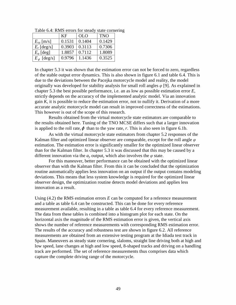
49

Table 6.4: RMS errors for steady state cornering KF OLO TNO Evy [m/s] 0.1531 0.1404 0.1429 Er [deg/s] 0.3903 0.3113 0.7306 Eφ [deg] 1.8857 0.7112 1.8089 Eϕ& [deg/s] 0.9796 1.1436 0.3525 In chapter 5.3 it was shown that the estimation error can not be forced to zero, regardless of the stable output error dynamics. This is also shown in figure 6.1 and table 6.4. This is due to the deviations between the Pacejka motorcycle model and reality, the model originally was developed for stability analysis for small roll angles φ [9]. As explained in chapter 5.3 the best possible performance, i.e. an as low as possible estimation error E, strictly depends on the accuracy of the implemented analytic model. Via an innovation gain K, it is possible to reduce the estimation error, not to nullify it. Derivation of a more accurate analytic motorcycle model can result in improved correctness of the estimations. This however is out of the scope of this research. Results obtained from the virtual motorcycle state estimators are comparable to the results obtained here. Tuning of the TNO MCSE differs such that a larger innovation is applied to the roll rate,ϕ& than to the yaw rate, r. This is also seen in figure 6.1b. As with the virtual motorcycle state estimators from chapter 5.2 responses of the Kalman filter and optimized linear observer are comparable, except for the roll angle φ estimation. The estimation error is significantly smaller for the optimized linear observer than for the Kalman filter. In chapter 5.3 it was discussed that this may be caused by a different innovation via the ay output, which also involves the φ state. For this maneuver, better performance can be obtained with the optimized linear observer than with the Kalman filter. From this it can be concluded that the optimization routine automatically applies less innovation on an output if the output contains modeling deviations. This means that less system knowledge is required for the optimized linear observer design, the optimization routine detects model deviations and applies less innovation as a result. Using (4.2) the RMS estimation errors E can be computed for a reference measurement and a table as table 6.4 can be constructed. This can be done for every reference measurement available, resulting in a table as table 6.4 for every reference measurement. The data from these tables is combined into a histogram plot for each state. On the horizontal axis the magnitude of the RMS estimation error is given, the vertical axis shows the number of reference measurements with corresponding RMS estimation error. The results of the accuracy and robustness test are shown in figure 6.2. All reference measurements are obtained from an extensive testing program at the Idiada test track in Spain. Maneuvers as steady state cornering, slaloms, straight line driving both at high and low speed, lane changes at high and low speed, 8-shaped tracks and driving on a handling track are performed. The set of reference measurements thus comprises data which capture the complete driving range of the motorcycle.

50

Figure 6.2: RMS state estimation errors from Kalman filter, optimized linear observer and TNO MCSE for the complete set of reference measurements

51

On the horizontal axis thus the RMS estimation error per state is shown, vertically the number of reference measurements with corresponding error is given. Accuracy is coupled to the mean estimation error, robustness to the standard deviation together with the maximum estimation errors (upper bounds in the histograms). Mean estimation

errors,E , and standard deviations,( )Eσ , for every state estimator and every state are shown in the legend.

Note that estimation errors in the r,ϕ& and φ states mainly arise because of the phase lag on the estimations, not because of strong deviations in magnitude of the estimations, see also figure 6.1c. Compensation of the phase lag will result in estimation errors near zero for these states. Estimation errors on the vy state however arise from erroneous model descriptions and can not be reduced when compensating for the phase lag. This can also be seen in figure 6.1c where the time history of the vy estimations differ strong from the measured vy.

It is also important to note that in the tuning process of the Kalman filter and optimized linear observer, estimation errors on the vy, r and φ state are weighted heavier than the estimation error on theϕ& state. This results in the relatively high estimation errors on theϕ& state in the lower left graph. The choice to weight theϕ& estimation error not as heavily is made because in future investigation the motorcycle states will be used for tyre force calculation. In thisϕ& does not play a role, see [9].

For all the other states, the Kalman filter and optimized linear observer behave similarly to the TNO MCSE. Due to the choices made in the tuning process, slightly better results can be obtained with the Kalman filter and optimized linear observer. Especially on the vy state and φ state much improvement is gathered concerning both the accuracy (lower mean estimation error) and the robustness (lower standard deviation on the estimation error).

With the tuning used here, the optimized linear observer outperforms the Kalman filter on all states, except for theϕ& state. The optimized linear observer accuracy on the vy, r and φ state is improved with respectively 36, 29 and 12% compared to the Kalman filter. Compared to the TNO MCSE accuracy improvements of respectively 44, 10 and 18% are obtained. It should be noted that with a different tuning of the TNO MCSE (less weighting on theϕ& state) these values will be lower.

Robustness of the Kalman filter and optimized linear observer are comparable to robustness of the TNO MCSE, standard deviations do not differ significantly. During all maneuvers the estimation errors stay bounded. For only a few maneuvers roll angle φ estimation errors are slightly higher than average, but still acceptable. The state estimators are checked for robustness to differences in the real motorcycle set-up. Multiple reference measurements are evaluated, where a different driver (10% mass increase) and different tyres, are used. Both state estimators are robust for these changes. A more thorough investigation, i.e. more reference measurements, is needed to be able to make a well-founded judgment in terms of robustness of the state estimators to parameter deviations.

52

6.3 Benchmark In order to validate the automatic tuning process for the Kalman filter and optimized linear observer, a benchmark is made on the real motorcycle. The analytic motorcycle model, implemented in the state estimators, has throughout the report been the Pacejka analytic motorcycle model from [9]. TNO recently developed its own analytic motorcycle model which is non-linear in the roll angle φ. A second challenging difference between the Pacejka model and the TNO model is that axis systems and sign conventions are defined differently: Pacejka uses the SAE axis system, the TNO model is expressed in the ISO axis system, see [9]. Table 6.5 shows the main differences between the models. Table 6.5: Differences between analytic motorcycle models Pacejka model TNO model

Mainframe Driver upper torso Front upper frame

Bodies

Front subframe

Mainframe

Tire model Linear Linear Roll angle range Linear, small angles Non-linear, complete range Axis system SAE ISO With states x and inputs u:

[ ] [ ]TxT

y vurvx δϕϕ == ,& (6.5)

The non-linear TNO motorcycle model is expressed by:

( )

[ ] ( )uxhray

uxfxT

y ,

,

==

=

ϕ&&

(6.6)

The equations of (6.6) are expressed in state space form (2.3) and implemented in the state estimators. System and gain matrix scheduling is performed as in (6.4). Similar operating points as in the previous chapter are chosen. Tuning of the Kalman filter and optimized linear observer gain matrices is done as described in section 6.1, using a similar reference measurements set. Results of the accuracy and robustness analysis with the linear, speed dependent state estimators for the real motorcycle are shown in figure 6.3. These results are obtained from the same reference measurements as in the accuracy and robustness analysis in the previous section, where the state estimators with the Pacejka motorcycle model are validated.

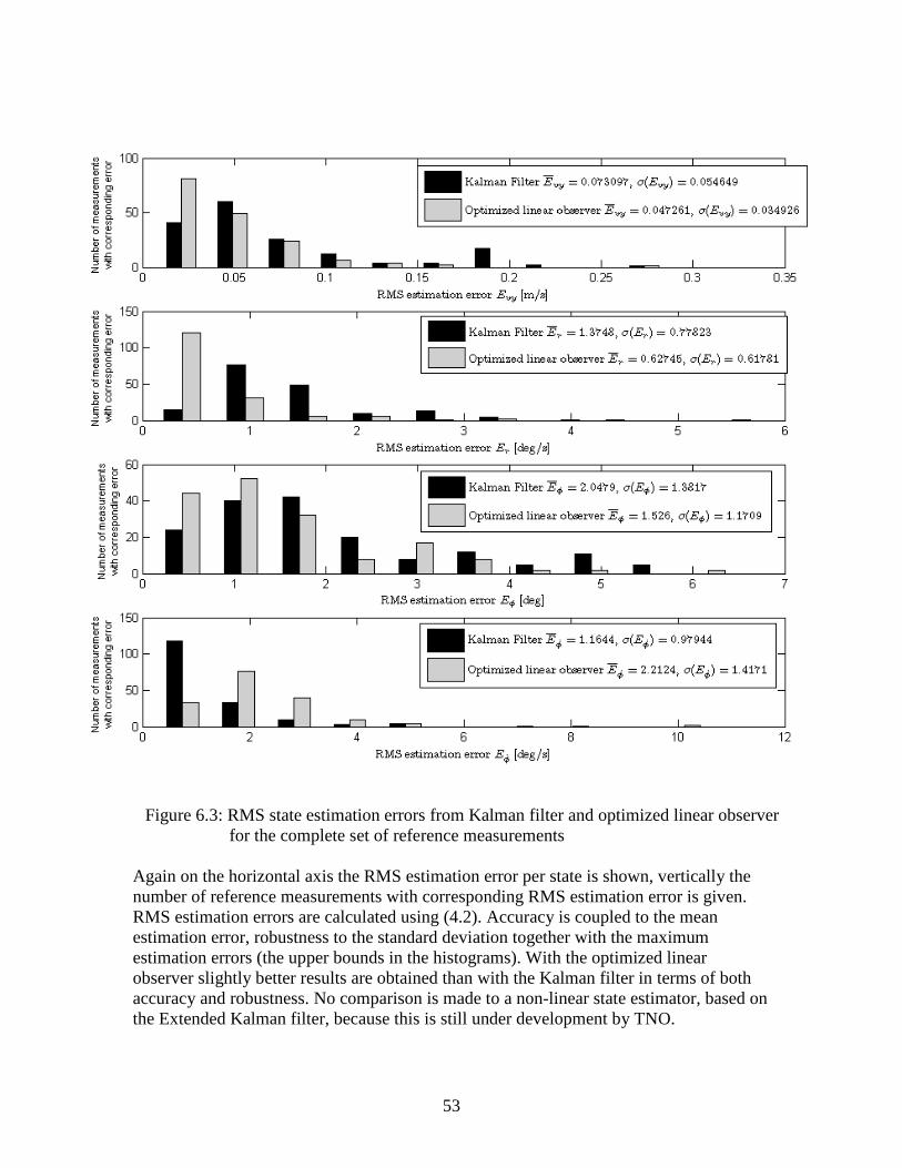
53

Figure 6.3: RMS state estimation errors from Kalman filter and optimized linear observer for the complete set of reference measurements

Again on the horizontal axis the RMS estimation error per state is shown, vertically the number of reference measurements with corresponding RMS estimation error is given. RMS estimation errors are calculated using (4.2). Accuracy is coupled to the mean estimation error, robustness to the standard deviation together with the maximum estimation errors (the upper bounds in the histograms). With the optimized linear observer slightly better results are obtained than with the Kalman filter in terms of both accuracy and robustness. No comparison is made to a non-linear state estimator, based on the Extended Kalman filter, because this is still under development by TNO.

54

Note again that in the tuning process, estimation errors on the vy, r and φ state are weighted higher than the estimation error on theϕ& state. This results in the relatively large estimation errors on theϕ& state in the lower left graph. The choice to weight theϕ& estimation error not as heavily is made because for future investigation the motorcycle states will be used for tyre force calculation. In thisϕ& does not play a role, see [9]. Compared to the results with the Pacejka analytic motorcycle model, figure 6.2, these set of state estimators perform less accurate. This is because parameters of the Pacejka model were tuned for the real motorcycle from which the reference measurements are obtained; parameters of the TNO model are not tuned for the real motorcycle yet. However, accuracy and robustness are still as desired. Note that this benchmark is not a final design for the linear state estimators using the TNO motorcycle model. The benchmark is only used to investigate if the outcome of the automatic tuning process is desirable, which is the case. The non-linear model used in this benchmark has lot more potential than considered here. A recommendation is to design state estimators which are designed at different operating conditions, for instance large roll angles. 6.4 Summary The automatic state estimator tuning process is used to tune a set of six discrete, speed dependent gain matrices for the Kalman filter and optimized linear observer. For each of the state estimators, within one day (2 GHz PC) a tuning of the gain matrices is made automatically.

With this tuning, for both the filter and observer similar accuracy and robustness is obtained as with the TNO motorcycle state estimator, based on the Extended Kalman filter. Due to deviations / simplifications in the analytic motorcycle model, it is not possible to force estimation errors to zero. Derivation of an analytic non-linear motorcycle model, together with tuning the parameters of the analytic model is advisable and will result in more accurate state estimation. An accuracy and robustness investigation shows that with the optimized linear observer slightly better results are obtained than with the linear Kalman filter and Extended Kalman filter. Partly, this can be addressed to decisions made in the tuning strategy. Overall however no significant differences occur between state estimates. A benefit of the optimized linear observer tuning method is that little knowledge about system or measurement noise is required. Based on reference measurements automatically a weighting is made, resulting in a robust and accurate tuning. A drawback of this method is that enough and representative reference measurements need to be available to obtain a robust tuning. With the automatic state estimator tuning process a benchmark is performed. Two new state estimators are designed, based on a linearized version of the non-linear analytic motorcycle model derived by TNO. The gain matrices for the Kalman filter and optimized linear observer are tuned by the automatic tuning process. Again an accurate and robust tuning is obtained. It is recommended to investigate, if better accuracy can be obtained when designing the Kalman filter and optimized linear observer for different operating conditions.

55

7. Conclusions and recommendations TNO has designed a motorcycle state estimator, based on an Extended Kalman filter, but tuning the state estimator is a very laborious task. The objective of this investigation is to find a solution to the laborious task of tuning the state estimator. An automatic tuning process is proposed, considering only linear state estimators. In this report, the development of the automatic state estimator tuning is described for a Kalman filter and an optimized linear observer. The following conclusions and recommendations summarize the results of this research. 7.1 Conclusions Model mismatch The analytic motorcycle model implemented in the state estimators, deviates from reality in terms of a different tyre behavior and a different roll angle range. Due to these model mismatches it is not straightforward to find an optimal tuning of the state estimators. Tuning the Kalman filter assumes knowledge of process and measurement noise. Process or measurement noise can not be reflected as model mismatch. However, mismatch can be taken into account by injecting uncertainty into the process noise and measurement noise covariance matrices Q and R. Note that this way model mismatch is only taken into account and not compensated for, and there will always be a non-zero state estimation error. Automatic tuning process The automatic tuning process tunes both a Kalman filter and optimized linear observer. Tuning of the state estimators requires a large number of calculations, up to 100000 calculations are required for obtaining a robust tuning. Due to the assumption of linear behavior of the motorcycle it is possible to perform simulations with linear state space models. These simulations demand far less computational effort than the conventional method, resulting in a fast tuning process. Tuning of the Kalman filter and optimized linear observer is performed fast and takes one day each, on a Pentium 2 Ghz system. Both state estimators behave accurate and robust. Optimized linear observer versus Kalman filter The proposed optimized linear observer is a stable state estimation technique which, amongst other things, can be applied to motorcycle state estimation for handling application. Tuning of the optimized linear observer can be performed fast (within one day on a Pentium 2 Ghz) and results in accurate and robust performance. Within bounds, the optimization algorithm compensates for model deviations and measurement noise. An accuracy and robustness analysis showed that, for a large set of reference measurements, with the optimized linear observer similar accuracy and robustness is obtained as with the Kalman filter and the reference motorcycle state estimator.

56

Virtual motorcycle state estimator For the virtual motorcycle two linear state estimators are designed: the Kalman filter and the optimized linear observer. Accuracy and robustness of the state estimators are compared to the TNO motorcycle state estimator. Only small differences between the non-linear TNO state estimator and the linear state estimators occur. The differences are mainly present due to a different tuning strategy.

Accuracy and robustness of both the Kalman filter and the optimized linear observer are as desired for all the reference measurements which are evaluated. With the optimized linear observer slightly better performance can be obtained than with the Kalman filter and TNO motorcycle state estimator.

The analytic motorcycle model, implemented in the state estimators, mainly differs from the virtual motorcycle in terms of tyre behavior and limited roll angle range. These differences result in estimation errors which can not be forced to zero. Accuracy of the state estimators is limited to the accuracy of the analytic motorcycle model. Deriving a more accurate analytic model is worthy and will improve accuracy of the state estimators.

Real motorcycle state estimator For a real motorcycle the Kalman filter and optimized linear observer are designed. The linear state estimators perform comparable to the TNO motorcycle state estimator. Small differences in accuracy can be imputed to the different tuning strategy for the state estimators. Due to the differences, in terms of tyre behavior and roll angle range, between the analytic motorcycle model and the real motorcycle it is not possible to force state estimation errors to zero. Accuracy and robustness however is as desired for both linear state estimators. This means that both the state estimators tuned by the automatic tuning process can be applied for real-time motorcycle state estimation. Due to the different tuning strategy slightly better performance is obtained with the optimized linear observer than with the Kalman filter.

Robustness experiments show that both motorcycle state estimators are robust for small differences in tyre characteristics and driver mass. With the experiments performed in this research again accuracy and robustness for both the Kalman filter and the optimized linear observer is as desired. A more thorough investigation, i.e. evaluation of more reference measurements, is needed to be able to make a well-founded judgment concerning robustness for other differences in the motorcycle settings.

Benchmark of automatic tuning process The automatic tuning process is benchmarked by implementing a second analytic motorcycle model in the state estimators. This analytic motorcycle model is a single mass model which is non-linear in the roll angle. Both state estimators perform accurate and behave robust. Both the Kalman filter and optimized linear observer obtained from the design process can be used for real-time application. Probably, for maneuvers containing larger roll angles, better accuracy is obtained when the non-linear model is linearized for other operating conditions than considered in this investigation.

57

7.2 Recommendations For future research of the linear motorcycle state estimator as well as for the non-linear TNO motorcycle state estimator the following recommendations are made. Improvement of analytic model The Pacejka analytic motorcycle model which is implemented in the state estimators mainly deviates from the virtual and real motorcycle in terms of tyre behavior and roll angle range. Due to these deviations it is not possible to obtain better accuracy than obtained here. Deriving a more accurate analytic motorcycle model is worthy. TNO already derived an extended, non-linear analytic motorcycle model. In the benchmark good results are obtained from the state estimators with the extended analytic motorcycle model implemented. By designing the state estimators for different operating points it is expected that accuracy can be increased significantly. Investigating which operating points to use is thus advisable. Output reduction During this research the same inputs ( δδ &

xv ) and outputs ( ϕ&ray ) are used for

the linear state estimator design as used with the TNO motorcycle state estimator. With fewer outputs the system can still be observable. For this reason it is interesting to investigate if with fewer outputs, for instance neglecting lateral acceleration ay, similar accuracy and robustness can be obtained as with the outputs used here. If this is the case on one hand a less complicated tuning is required and on the other hand cheaper sensor instrumentation is needed. The same of course also holds for a reduction of inputs. Outputs used as input, reduced order observer For the state estimators both the inputs and outputs are measured. The inputs are used to make the state estimations, the outputs are used to correct these estimations. If an output signal contains very little to no measurement noise, it can also be used as an input instead. For instance, the yaw rate r signal can be extracted from the output vector and added to the input vector. This way yaw rate no longer needs to be estimated using an analytic model, but is available as a measured input directly. It is interesting to investigate if this method can result in better performance and a faster tuning. Parameter estimation Knowledge of the vehicle mass and tyre characteristics is very important for the state estimator to perform accurately. In this research fixed mass and fixed tyre characteristics are assumed and incorporated in the analytic motorcycle model. A brief robustness analysis has proven that the estimators are robust for small deviations in these parameters, for the reference measurements available. For more severe deviations, serious robustness issues can occur. For this reason it is useful to extend the state vector with important parameters, for example including a mass and a friction state. An application of joint parameter and state estimation is described in [31].

58

Modelling of error It is known that differences between the analytic motorcycle model and the virtual and real motorcycle result in inaccurate state estimates. It is interesting if it is possible to model this estimation error as a function of estimated state and measured input. If this is possible, the state estimates can be compensated with this function. This is done best by comparing open loop responses. A problem that arises is that the analytic motorcycle model is an unstable model. Note that this method is close to deriving a more accurate analytic motorcycle model. Tuning with respect to tyre forces In the automatic tuning process the state estimators are tuned by comparing the estimated states with the measured states. Real-time evaluation of the lateral tyre forces is interesting, for these can be used to prevent accidents or for future control systems. Tuning the state estimators for an as low as possible tyre force estimation error thus is interesting. However, tyre forces can not be measured, tyre axle forces can. If the real motorcycle is equipped with axle force sensors, the state estimators can be tuned by comparing estimated axle forces with measured axle forces. If correct axle force estimation is possible, it is plausible that correct lateral tyre force estimation is possible.

59

Bibliography [1] Insurance Information Institute,

http://www.iii.org/media/hottopics/insurance/motorcycle/, march 2008 [2] European Commission – Road safety,

http://ec.europa.eu/transport/roadsafety/road_safety_observatory/care_reports_en.htm, april 2008

[3] G.F. Franklin, J.D. Powell, A. Emami-Naeini, Feedback Control of Dynamic Systems, Prentice Hall, New Jersey, 2002.

[4] A. Teerhuis, S.T.H. Jansen, Development of a Motorcycle State Estimator concept for cornering behavior using a Multi-Body simulation model, TNO report 07.OR.IS.045/AT, TNO, 2007

[5] R.E. Kalman, A new approach to linear filtering and prediction problems, Transactions of the ASME, Journal of Basic Engineering, Vol 83, pp95-108, 1961.

[6] D.G. Luenberger, Observing the state of a linear system, IEEE Trans. on Military Electronics, Vol. MIL-8, pp.74-80, 1964

[7] R.S. Sharp, The stability and control of motorcycles, Journal of mechanical engineering science, Vol 13, pp.5, 1971

[8] C. Koenen, The dynamic behaviour of a motorcycle when running straight ahead and when cornering, PhD thesis, Delft University of Technology, 1983

[9] H. B. Pacejka, Tyre and vehicle dynamics, Butterworth–Heinemann, Amsterdam 2002.

[10] H.W. Sorenson, Least-squares estimation: from Gauss to Kalman, IEEE, Vol 7, pp63-68, July 1970.

[11] D.G. Luenberger, Observers for multivariable systems, IEEE Trans. on Automatic Control, Vol. AC-11 (2), pp.190-197, 1966

[12] D.G. Luenberger, An introduction to observers, IEEE Trans. on Automatic Control, Vol. AC-16 (6), pp.596-602, 1971

[13] B.D.O. Anderson, J.B. Moore, Optimal Filtering, Prentice-Hall, Englewood Cliffs, 1979

[14] A. Gelb, Applied optimal estimation, The Analytic Sciences Corporation, United States of America, 1974.

[15] W.J.M. Rankine, On the dynamical principles of the motion of velocipedes, The Engineer, pp. 2,79,129,153,175, 1869/1870

[16] F.J.W. Whipple, The stability of the motion of a bicycle, Q.J. Pure Applied Mathematics, Vol. 30, pp.312-348, 1899

[17] D.J.N. Limebeer, R.S. Sharp, Bicycles, Motorcycles and Models, IEEE control systems magazine, Vol 26(5), pp.34-61, October 2006

[18] J.P. Meijaard, J.M. Papadopoulus, A. Ruina, A.L. Schwab, Linearized dynamics equations for the balance and steer of a bicycle: a benchmark and review, Proc. R. Soc, A, Vol. 463, pp.1955-1982, 2007

[19] R.D. Roland, Computer simulation of bicycle dynamics, Proc. ASME Symp. Mechanics Sport, pp.35-83, 1973

60

[20] E. Döhring, Stability of single-track vehicles, Institut für Fahrzeugtechnik, Technische Hochschule Braunschweig, Forschung Ing. –Wes, Vol 21(2), pp.50-62, 1955

[21] J.L. Neimark, N.A. Fufaev, Dynamics of nonholonomic systems, Amer. Math. Soc. Translations Math. Monographs, Vol 33, 1972

[22] R.S. Sharp and C.J. Alstead, The influence of structural flexibilities on the straight-running stability of motorcycles, Vehicle system dynamics, Vol 9, pp.327-357, 1980

[23] M.K. Verma, R.A. Scott, L. Segel, Effect of frame compliance on lateral dynamics of motorcycles, Vehicle system dynamics, Vol. 9(4), pp.181-205, 1980

[24] P.T.J. Spierings, The effects of lateral front fork flexibility on the vibrational modes of straight running single-track vehicles, Vehicle system dynamics, Vol 10, pp.21-35, 1981

[25] R.S. Sharp, The lateral dynamics of motorcycles and bicycles, Vehicle system dynamics, Vol 14, pp.265-283, 1985

[26] R. Berritta, F. Biral, S. Garbin, Evaluation of motorcycle handling with multibody modelling and simulation. High tech engines and cars, 6th international conference, May 25th-26th 2000

[27] V. Cossalter, R. Lot, A motorcycle multi-body model for real time simulations based on the natural coordinates approach, Vehicle system dynamics, Vol 37(6), pp.423-447, 2002

[28] W. Versteden, Improving a tyre model for motorcycle simulations, MSc thesis, Eindhoven, University of technology, 2005

[29] W.D. Versteden, M.F.A. Lammers, S.T.H. Jansen, A.P. Teerhuis, Benchmark of motorcycle simulation models, TNO report 06.MR.IS.035.1/WV, TNO, 2007

[30] J. Zuurbier, P. Bremmer, State Estimation for Integrated Vehicle Dynamics Control, Proceedings of AVEC 2002, Hiroshima (Japan), 2002

[31] P.M. Siegrist, P.R. McAree, Tyre-force estimation by Kalman inverse filtering: applications to off-highway mining trucks, Vehicle system dynamics, Vol(44)12, pp. 921-937, December 2006.

[32] S.F. Schmidt, Computational Techniques in Kalman Filtering, NATO Advisory Group for Aerospace Research and Development, London, February 1970

61

A. Vehicle equations of motion

( ) ( ) ( ) ( )( ) ( )( )Izz

IxzIxzIzzIxx

FyFyhbFyaFyIzzIxzBBmghCCh

m

murFyFyvy 22 2

2121212121

−+−

+++++++−++−+=

εε

εϕϕ &&

(A.1)

( ) ( ) ( ) ( )( ) ( )

IzzIxzIxzIzzIxx

bFyaFyIxxFyFyhBBmghCCIzzIxz

r22 2

21212121

−+−

++++++++−=

εε

ϕϕε &&

(A.2)

ϕϕ && = (A.3)

( ) ( )( ) ( )

IzzIxzIxzIzzIxx

FyFyhbFyaFyIzzIxzBBCCmgh

22 2

2121)21(21

−+−

+−++−+−−−=

εε

εϕϕϕ

&&&

(A.4)

m

FyFyhurva yy

21+=++= ϕ&&& (A.5)

rr = (A.6) With tyre forces:

( ) ( ) ( )

+−−

+−−

+−= arvu

Barvu

BEarvu

BCDFy yyy

1arctan

11arctansin1 δδδ

(A.7)

( ) ( ) ( )

−−−

−−−

−−= brvu

Bbrvu

BEbrvu

BCDFy yyy

1arctan

11arctansin2

(A.8)

62

B. Gain matrices and closed loop pole locations Pacejka analytic motorcycle state estimators

±−−−

=

−−−

−−−

=

−±−

−=

−−−

−−−

=

−−−−

=

−−−

−−−

=

−−−−

=

−−−

−−−

=

−−−−

=

−−

−−

=

±−−−

=

−−

−−

=

i

K

iK

K

K

K

i

K

KFKF

KFKF

KFKF

KFKF

KFKF

KFKF

68.3316

68.26

03.0

,

4622.10409.00093.0

4618.3248158.10646.0

1582.183750.3043308.0

1878.1431470.250798.1

44.316

1.3225.79

03.0

,

6684.10398.00080.0

3663.1380333.21044.0

3330.201959.3023676.0

0459.21605.207598.0

1190.319

1083.314

5182.68

0462.0

,

8576.00542.00324.0

6555.3225065.05211.0

0652.59776.2968628.3

0292.801178.98609.6

8184.318

4612.312

1854.52

0311.0

,

4644.10433.00093.0

1983.3304189.01032.0

1889.46238.2935111.0

0692.1287706.90390.1

1976.319

7998.310

5437.78

0313.0

,

4579.10467.00093.0

6643.3554272.01412.0

2723.40465.2836773.0

8476.1204267.4039.1

11.23.320

72.94

05.0

,

6460.10470.00081.0

2759.32143.1029.0

2997.140613.2531547.1

6846.147013.11407.0

120120

100100

8080

6060

4040

2020

λ

λ

λ

λ

λ

λ

63

±−−−

=

−−

−−

=

±−−−

=

−−−

−−

=

±−−−

=

−−−

−−

=

±−−−

=

−−−

−−

=

±−−−

=

−−−

−−

=

−±−

−=

−−−

−

=

i

K

i

K

i

K

i

K

i

K

iK

FLOFLO

FLOFLO

FLOFLO

FLOFLO

FLOFLO

FLOFLO

6.14582.143

71.41

02.0

,

7235.00157.00008.0

4188.1112005734.6

4439.1082008604.5

2002005542.3

9.1424.150

02.37

02.0

,

7298.03212.00009.0

8039/1212004947.6

8451.1052006437.4

2002003622.4

8.17053.189

68.56

002.0

,

9209.01459.00003.0

2002001760.7

0628.1312008468.6

0050.1362009691.1

7.14496.164

23.106

01.0

,

6881.05407.00004.0

2002000466.8

5861.902001597.8

1642.1452006293.3

4.1488.157

41.125

03.0

,

5399.01357.00004.0

2002002634.7

5862.922001326.7

9723.1392004883.4

16.424

9.24318.27

02.0

,

5216.01681.00004.0

2002003510.8

2002009062.9

8981.1822001307.5

120120

100100

8080

6060

4040

2020

λ

λ

λ

λ

λ

λ

64

C. Matlab Kalman filter Analytic state space matrices are obtained with: A = jacobian(f,x), B = jacobian(f,u), C = jacobian(h,x), D = jacobian(h,u) In which f contains the state differential equations, x contains the states, u contains the inputs and h contains the sensor model. With knowledge of the system matrices A and C and the noise covariance matrices Q and R, the Kalman gain KKF can be computed using Riccati with: [P, Efilter] = care (A’,C’,Q,R) K_KF = P*C’*inv(R) Closed loop eigenvalues of the Kalman filter are given in Efilter. For other estimators, typically closed loop eigenvalues are determined with: Labda = eig(A-K*C) Luenberger observer For a single output system the gain matrix for the Luenberger observer can be computed using both the acker or place commands: K = place(A’,C’,labda)’ or with: K = acker(A’,C’,labda)’ In this labda is the vector containing the desired closed loop pole locations of the observer. System matrices A and C are obtained from the jacobians of the system and output equations as described for the Kalman filter. Extended Kalman filter Contrary to the gain matrices of the linear state estimators, the Extended Kalman filter gain matrix is determined real-time. For this jacobians of both the system and output equations are needed. The overview of the EKF gain matrix determination is shown in the upper graph, the dynamic Riccati equation is shown in the lower graph. This is implemented in the P-subsystem of the overview.

65

1

Out1

Rinv_EKF

inv(R)1

C_EKF

To Workspace2

A_EKF

To Workspace1

K_EKF

To Workspace

H

H'

P

inv (R)

PH'inv (R)HP

PH' inv(R) HP

FP

PF'

PH'inv (R)HP

P

P

inv (R)

P

H'

K

K

xH

H'

H

[P_ekf]

Goto

[P_ekf]

From2

[P_ekf]

From1P

F

F'

FP

PF'

FP, PF'

xF

F'

F

1

In1

DP P1

P

Q_EKF

Q

1s

Integrator

3

PH'inv(R)HP

2

PF'

1

FP

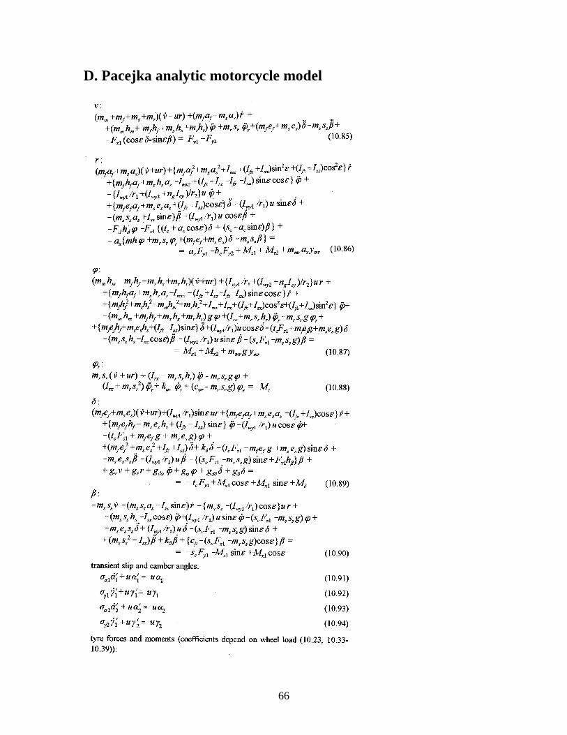
66

D. Pacejka analytic motorcycle model

67