Descriptive Statistics

Descriptive Statistics Krupnik Estate Agents

Anthony J. Evans Associate Professor of Economics, ESCP Europe

www.anthonyjevans.com

London, February 2015

(cc) Anthony J. Evans 2015 | http://creativecommons.org/licenses/by-nc-sa/3.0/

Weekly prices of studio apartments in West Hampstead

2

425

440

450

465

480

510

575

430 440

450

470

485

515 575

430

440

450

470

490

525

580

435

445

450

472

490

525

590

435

445

450

475

490

525

600

435

445

460

475

500

535

600

435

445

460

475

500

549

600

435

445

460 480 500

550

600

440 450

465

480

500

570

615

440

450 465

480

510

570

615

Weekly prices of studio apartments in West Hampstead (2)

•  The first task is to order the data set

3

425 430 430 435 435 435 435 435 440 440 440 440 440 445 445 445 445 445 450 450 450 450 450 450 450 460 460 460 465 465 465 470 470 472 475 475 475 480 480 480 480 485 490 490 490 500 500 500 500 510 510 515 525 525 525 535 549 550 570 570 575 575 580 590 600 600 600 600 615 615

Foundations of descriptive statistics

Measures of data

Location

Dispersion

Description

•  A “typical” or average value •  Used to summarise the distribution

•  The spread or variability of the data •  Appreciate the differences in the data

4

Measures of Location: Mean

•  The mean of a data set is the summation of all individual values, divided by the number of observations

Sample Population

5 Notice the use of Greek/upper case for populations and English/lower case for samples

€

x =xi∑n

=34,35670

= 490.80€

µ =x∑i

N

€

x =x∑i

n

Measures of Location: Mean

•  The mean of a data set is the summation of all individual values, divided by the number of observations

Sample Population

6 Notice the use of Greek/upper case for populations and English/lower case for samples

€

x =xi∑n

=34,35670

= 490.80€

µ =x∑i

N

€

x =x∑i

n

Measures of Location: Median

•  The median of a data set is the value that divides the lower half of the distribution from the higher half

•  The median is the middle observation –  i.e. the (n+1)/2th observation –  In this case, 71/2 = 35.5th observation

•  If there are an even number of observations, take the mean of both middle values

•  Median = 475

7

425 430 430 435 435 435 435 435 440 440

440 440 440 445 445 445 445 445 450 450

450 450 450 450 450 460 460 460 465 465

465 470 470 472 475 475 475 480 480 480

480 485 490 490 490 500 500 500 500 510

510 515 525 525 525 535 549 550 570 570

575 575 580 590 600 600 600 600 615 615

Measures of Location: Median

•  The median of a data set is the value that divides the lower half of the distribution from the higher half

•  The median is the middle observation –  i.e. the (n+1)/2th observation –  In this case, 71/2 = 35.5th observation

•  If there are an even number of observations, take the mean of both middle values

•  Median = 475

8

425 430 430 435 435 435 435 435 440 440

440 440 440 445 445 445 445 445 450 450

450 450 450 450 450 460 460 460 465 465

465 470 470 472 475 475 475 480 480 480

480 485 490 490 490 500 500 500 500 510

510 515 525 525 525 535 549 550 570 570

575 575 580 590 600 600 600 600 615 615

Measures of Location: Mode

•  The mode of a data set is the value that occurs with the greatest frequency.

•  If the data have exactly two modes, the data are bimodal •  If the data have more than two modes, the data are

multimodal

•  Mode = 450

9

425 430 430 435 435 435 435 435 440 440

440 440 440 445 445 445 445 445 450 450

450 450 450 450 450 460 460 460 465 465

465 470 470 472 475 475 475 480 480 480

480 485 490 490 490 500 500 500 500 510

510 515 525 525 525 535 549 550 570 570

575 575 580 590 600 600 600 600 615 615

Measures of Location: Mode

•  The mode of a data set is the value that occurs with the greatest frequency.

•  If the data have exactly two modes, the data are bimodal •  If the data have more than two modes, the data are

multimodal

•  Mode = 450

10

425 430 430 435 435 435 435 435 440 440

440 440 440 445 445 445 445 445 450 450

450 450 450 450 450 460 460 460 465 465

465 470 470 472 475 475 475 480 480 480

480 485 490 490 490 500 500 500 500 510

510 515 525 525 525 535 549 550 570 570

575 575 580 590 600 600 600 600 615 615

Measures of Location: Using Excel

11

Measures of Location: Percentiles

•  The median is also known as the 50th percentile •  The p th percentile of a data set is a value such that

p percent of the items take on this value or less, and (100 - p) percent of the items take on this value or more –  Arrange the data of ‘n’ items in ascending order –  Compute index i, the position of the pth

percentile

–  If i is not an integer, round up. The p th percentile is the value in the i th position.

–  If i is an integer, the p th percentile is the average of the values in positions i and i +1

•  I is the position of the p percentile

12 €

i =p100"

# $

%

& ' n

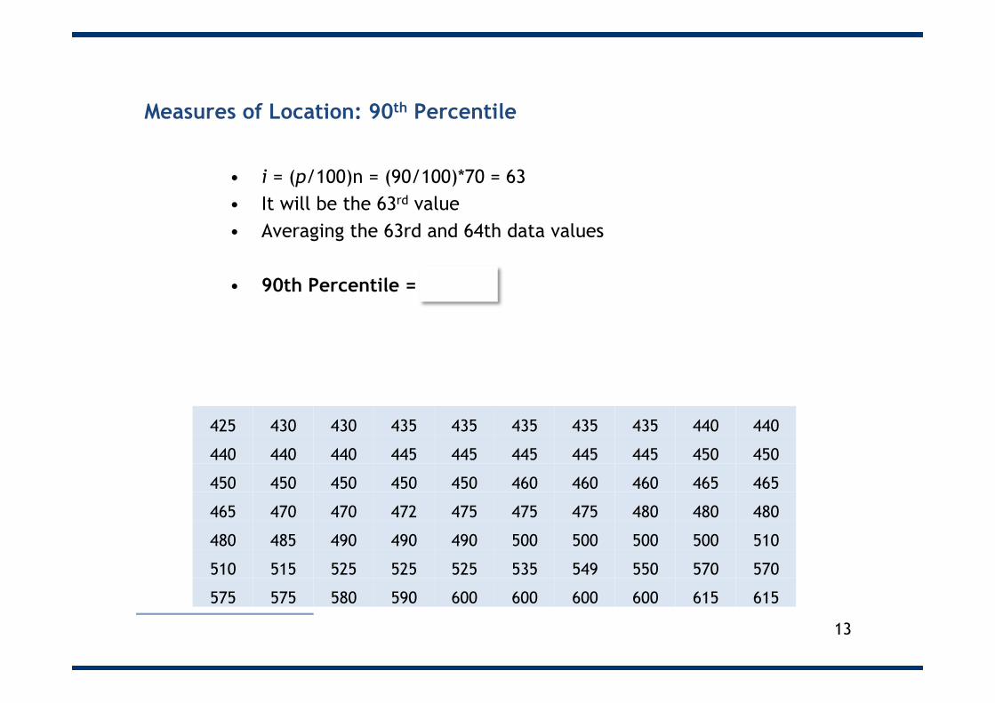
Measures of Location: 90th Percentile

•  i = (p/100)n = (90/100)*70 = 63 •  It will be the 63rd value •  Averaging the 63rd and 64th data values

•  90th Percentile = 585

13

425 430 430 435 435 435 435 435 440 440

440 440 440 445 445 445 445 445 450 450

450 450 450 450 450 460 460 460 465 465

465 470 470 472 475 475 475 480 480 480

480 485 490 490 490 500 500 500 500 510

510 515 525 525 525 535 549 550 570 570

575 575 580 590 600 600 600 600 615 615

Measures of Location: 90th Percentile

•  i = (p/100)n = (90/100)*70 = 63 •  It will be the 63rd value •  Averaging the 63rd and 64th data values

•  90th Percentile = 585

14

425 430 430 435 435 435 435 435 440 440

440 440 440 445 445 445 445 445 450 450

450 450 450 450 450 460 460 460 465 465

465 470 470 472 475 475 475 480 480 480

480 485 490 490 490 500 500 500 500 510

510 515 525 525 525 535 549 550 570 570

575 575 580 590 600 600 600 600 615 615

Measures of Location: 25th Percentile

•  i = (p/100)n = (25/100)*70 = 17.5 •  It will be the 18th value

•  25th Percentile = 445

15

425 430 430 435 435 435 435 435 440 440

440 440 440 445 445 445 445 445 450 450

450 450 450 450 450 460 460 460 465 465

465 470 470 472 475 475 475 480 480 480

480 485 490 490 490 500 500 500 500 510

510 515 525 525 525 535 549 550 570 570

575 575 580 590 600 600 600 600 615 615

Measures of Location: 25th Percentile

•  i = (p/100)n = (25/100)*70 = 17.5 •  It will be the 18th value

•  25th Percentile = 445

16

425 430 430 435 435 435 435 435 440 440

440 440 440 445 445 445 445 445 450 450

450 450 450 450 450 460 460 460 465 465

465 470 470 472 475 475 475 480 480 480

480 485 490 490 490 500 500 500 500 510

510 515 525 525 525 535 549 550 570 570

575 575 580 590 600 600 600 600 615 615

GDP of UN member countries

17 On average, how many legs do English people have?

Measures of Dispersion

•  in choosing supplier A or supplier B we should consider not only the average delivery time for each, but also the variability in delivery time for each

A

Mean = 0

Freq

uenc

y

B

Mean = 0

Freq

uenc

y

18

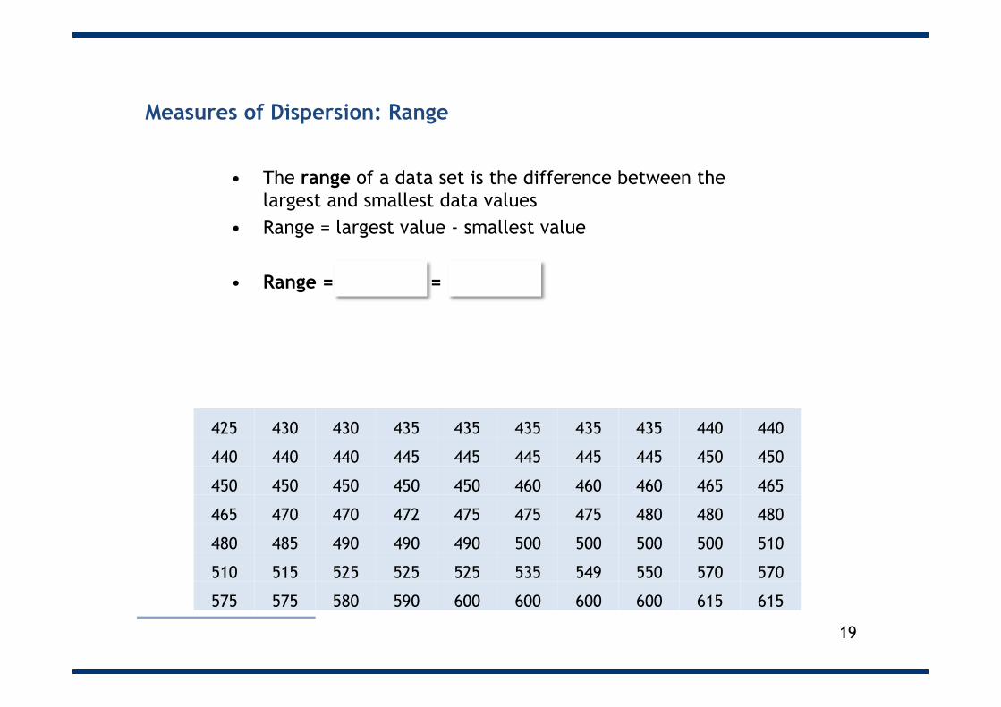
Measures of Dispersion: Range

•  The range of a data set is the difference between the largest and smallest data values

•  Range = largest value - smallest value

•  Range = 615 - 425 = 190

19

425 430 430 435 435 435 435 435 440 440

440 440 440 445 445 445 445 445 450 450

450 450 450 450 450 460 460 460 465 465

465 470 470 472 475 475 475 480 480 480

480 485 490 490 490 500 500 500 500 510

510 515 525 525 525 535 549 550 570 570

575 575 580 590 600 600 600 600 615 615

Measures of Dispersion: Range

•  The range of a data set is the difference between the largest and smallest data values

•  Range = largest value - smallest value

•  Range = 615 - 425 = 190

20

425 430 430 435 435 435 435 435 440 440

440 440 440 445 445 445 445 445 450 450

450 450 450 450 450 460 460 460 465 465

465 470 470 472 475 475 475 480 480 480

480 485 490 490 490 500 500 500 500 510

510 515 525 525 525 535 549 550 570 570

575 575 580 590 600 600 600 600 615 615

Measures of Dispersion: Interquartile range

•  The interquartile range of a data set is the difference between the first and third quartiles

•  Q1 = 25th percentile = 445 (from before) •  Q3 = 75th percentile = 525

•  Interquartile range = 525 - 445 = 80

21

425 430 430 435 435 435 435 435 440 440

440 440 440 445 445 445 445 445 450 450

450 450 450 450 450 460 460 460 465 465

465 470 470 472 475 475 475 480 480 480

480 485 490 490 490 500 500 500 500 510

510 515 525 525 525 535 549 550 570 570

575 575 580 590 600 600 600 600 615 615

€

i = (p100 )n

Measures of Dispersion: Interquartile range

•  The interquartile range of a data set is the difference between the first and third quartiles

•  Q1 = 25th percentile = 445 (from before) •  Q3 = 75th percentile = 525

•  Interquartile range = 525 - 445 = 80

22

425 430 430 435 435 435 435 435 440 440

440 440 440 445 445 445 445 445 450 450

450 450 450 450 450 460 460 460 465 465

465 470 470 472 475 475 475 480 480 480

480 485 490 490 490 500 500 500 500 510

510 515 525 525 525 535 549 550 570 570

575 575 580 590 600 600 600 600 615 615

€

i = (p100 )n

Measures of Dispersion: Variance

•  The variance is a measure of variability that utilizes all the data.

•  It is based on the difference between the value of each observation (xi) and the mean (x BAR for a sample, and m for a population)

•  The variance is the average of the squared differences between each data value and the mean.

€

s2

=(xi−x )2∑

n−1

€

σ 2 =(xi −µ)2∑N

23

Sample Population

Measures of Dispersion: Standard Deviation

•  The standard deviation of a data set is the square root of the variance.

•  It is more easily comparable to the mean than the variance – standard deviation measures the spread about the mean using the original (not squared) scale

•  It ties into the Normal Distribution*

€

s = s2

€

σ = σ 2

Sample Population

* See lecture 4. Probability Distributions 24

€

s =(xi −x )2∑

n−1

What is the standard deviation?

25

i xi xi - x' (xi - x')2 1 425 -65.8 4329.64 2 440 -50.8 2580.64 3 450 -40.8 1664.64 4 465 -25.8 665.64 5 480 -10.8 116.64 6 510 19.2 368.64 7 575 84.2 7089.64 8 430 -60.8 3696.64 9 440 -50.8 2580.64

10 450 -40.8 1664.64

65 450 -40.8 1664.64 66 465 -25.8 665.64 67 480 -10.8 116.64 68 510 19.2 368.64 69 570 79.2 6272.64 70 615 124.2 15425.64

sum 206,735.20 /(n-1) 2,996.16

sqrt 54.74

Measures of Dispersion: Examples

•  Variance

•  Standard Deviation

€

s2 =

( xi −x )2∑n−1

= 2, 996

74.5429962 === ss26

Measures of Dispersion: z Score

•  The z - score is the standardised value •  It denotes the number of standard deviations a

data value xi is from the mean

•  A data value less than the sample mean will have a z-score less than zero

•  A data value greater than the sample mean will have a z -score greater than zero

€

zi =xi − x

s

27

Measures of Dispersion: z Score for smallest value

•  z-Score of Smallest Value (425)

•  Standardized Values for Apartment Rents:

z x xsi=−

=−

= −425 490 8054 74

1 20..

.

28

425 430 430 435 435 435 435 435 440 440

440 440 440 445 445 445 445 445 450 450

450 450 450 450 450 460 460 460 465 465

465 470 470 472 475 475 475 480 480 480

480 485 490 490 490 500 500 500 500 510

510 515 525 525 525 535 549 550 570 570

575 575 580 590 600 600 600 600 615 615

Measures of Dispersion: z Score for smallest value

•  z-Score of Smallest Value (425)

•  Standardized Values for Apartment Rents:

z x xsi=−

=−

= −425 490 8054 74

1 20..

.

29

425 430 430 435 435 435 435 435 440 440

440 440 440 445 445 445 445 445 450 450

450 450 450 450 450 460 460 460 465 465

465 470 470 472 475 475 475 480 480 480

480 485 490 490 490 500 500 500 500 510

510 515 525 525 525 535 549 550 570 570

575 575 580 590 600 600 600 600 615 615

Measures of Dispersion: Outliers

•  An outlier is an unusually small or unusually large value in a data set –  It might be an incorrectly recorded data value –  It might be a data value that was incorrectly included

in the data set –  It might be a correctly recorded data value that

belongs in the data set!

•  A data value with a z-score less than -3 or greater than +3 might be considered an outlier

30

Summary

•  There are two main ways to get feel for a set of numbers (a distribution) – location and dispersion

•  The mean and the standard deviation are the most frequent measures of location and dispersion but it’s important to understand the alternatives

31

•  This presentation forms part of a free, online course on analytics

•  http://econ.anthonyjevans.com/courses/analytics/

32