Descriptive and Inferential Statistics

-1-

Descriptive and Inferential Statistics

Paul A. Jargowsky and Rebecca YangUniversity of Texas at Dallas

I. Descriptive StatisticsII. Inferential StatisticsIII. Cautions and Conclusions

GLOSSARY

bootstrapping – a re-sampling procedure to empirically estimate standard errors. central tendency – the dominant quantitative or qualitative trend of a given variable (commonly

measured by the mean, the median, the mode and related mesures).

confidence interval – a numeric range, based on a statistic and its sampling distribution, thatcontains the population parameter of interest with a specified probability.

data – a plural noun referring to a collection of information in the form of variables andobservations.

descriptive statistics – any of numerous calculations which attempt to provide a concisesummary of the information content of data (for example, measures of central tendency,measures of dispersion, etc.).

dispersion – the tendency of observations of a variable to deviate from the central tendency(commonly measured by the variance, the standard deviation, the interquartile range,etc.).

inferential statistics – the science of drawing valid inferences about a population based on asample.

level of measurement – a characterization of the information content of a variable; for example,variables may be qualitative (nominal or interval) or quantitative (interval or ratio).

parameter – the true value of a descriptive measure in the population of interest.

population the total collection of actual and/or potential realizations of the unit of analysis,whether observed or not.

-2-

sample – a specific, finite, realized set of observations of the unit of analysis.

sampling distribution – a theoretical construct describing the behavior of a statistic in repeatedsamples.

statistic – a descriptive measure of calculated from sample data to serve as an estimate of anunknown population parameter.

unit of analysis – the type of thing being measured in the data, such as persons, families,households, states, nations, etc.

There are two fundamental purposes to analyzing data: the first is to describe a large number of

data points in a concise way by means of one or more summary statistics; the second is to draw

inferences about the characteristics of a population based on the characteristics of a sample.

Descriptive statistics characterize the distribution of a set of observations on a specific variable

or variables. By conveying the essential properties of the aggregation of many different

observations, these summary measures make it possible to understand the phenomenon under

study better and more quickly than would be possible by studying a multitude of unprocessed

individual values. Inferential statistics allow one to draw conclusions about the unknown

parameters of a population based on statistics which describe a sample from that population.

Very often, mere description of a set of observations in a sample is not the goal of research. The

data on hand are usually only a sample of the actual population of interest, possibly a minute

sample of the population. For example, most presidential election polls only sample about 1,000

individuals, and yet the goal is to describe the expected voting behavior of 100 million or more

-3-

potential voters.

I. Descriptive Statistics.

A number of terms have specialized meaning in the domain of statistics. First, there is

the distinction between populations and samples. Populations can be finite or infinite. An

example of the former is the population of the United States on April 15, 2000, the date of the

Census. An example of the latter is the flipping of a coin, which can be repeated in theory ad

infinitum. Populations have parameters, which are fixed but usually unknown. Samples are

used to produce statistics, which are estimates of population parameters. This section discusses

both parameters and statistics, and the following section discusses the validity of using statistics

as estimates of population parameters.

There are also a number of important distinctions to be made about the nature of the data

to be summarized. The characteristics of data to be analyzed limit the types of measures that can

be meaningfully employed. Section B below addresses some of the most important of these

issues.

A. Forms of Data

All statistics are based on data, a plural noun, which are comprised of one or more

variables that represent the characteristics of one or more of the type of thing being studied. A

variable consists of a defined measurement. The type of thing upon which the measurements are

taken is called the unit of analysis. For example, the unit of analysis could be individual people,

but it could also be families, households, neighborhoods, cities, nations, or galaxies.

-4-

The collection of all measurements for one realization of the unit of analysis is typically

called an observation. If there are n observations and k variables, then the data set can be thought

of as a grid with n x k total items of information, although more complex structures are possible.

It is absolutely central to conducting and interpreting data analysis to be clear about the

unit of analysis. For example, if one observes that 20 percent of all crimes are violent in nature,

it does not imply that 20 percent of all criminals are violent criminals. Crimes, though obviously

related, are simply a different unit of analysis than criminals; a few really violent criminal could

be committing all the violent crimes, so that less than 20 percent of criminals are violent in

nature.

1. Levels of Measurement.

A variable is something that varies between observations, at least potentially, but not all

variables vary in the same way. The specific values which a variable can take on, also known as

attributes, convey information about the differences between observations on the dimension

measured by the variable. So, for example, you and I differ on the variable income if my income

is $100,000 and yours is $200,000. We also differ on the variable sex if I am male and you are

female. But the nature of the information conveyed by the two variables is quite different. For

one thing, we can rank our incomes, but not our sexes. We can say that you have twice as much

income as me, but there is no comparable statement regarding our sexes. There are four main

types of variables, in two distinct categories, ordered from the highest level of measurement to

the lowest.

-5-

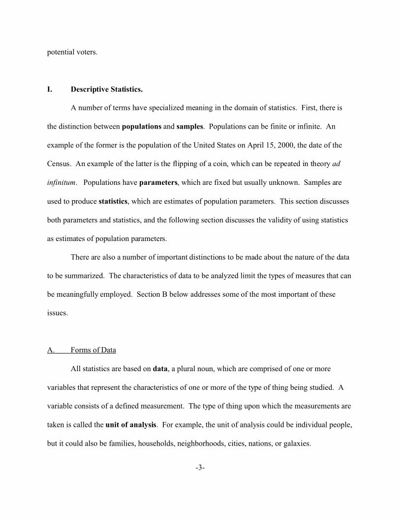
C Quantitative variables are measured on a continuous scale. In theory, there arean infinite number of potential attributes for a quantitative variable.

C Ratio variables are quantitative variables which have a true zero. Theexistence of a true zero makes the ratio of two measures meaningful. Forexample, we can say that your income is twice my income because$200,000/$100,000 = 2.

C Interval variables are quantitative as well, but lack a true zero. Temperature is a common example: the zero point is arbitrary and in factdiffers between the Centigrade and Fahrenheit systems. It doesn’t makesense to say that 80° F is twice as hot as 40° F; in Centigrade the ratiowould be 6; neither ratio is meaningful.

C Qualitative (or categorical) variables are discrete; that is, a measurementconsists of assigning an observation to one or more categories. The attributes ofthe variable consist of the finite set of potential categories. The set of categoriesmust be mutually exclusive and collectively exhaustive. That is, each observationcan be assigned to one and only one category.

C In ordinal variables, the categories have an intrinsic order. Sears andRoebuck, for example, classifies its tools in three categories: good, better,best. They have no numerical relation; we don’t know if better is twice asgood as good. But they clearly can be ordered.

C In nominal variables, the categories have no intrinsic order. A variablefor Religion, for example, could consist of the following set of categories:Catholic, Protestant, Hindu, Muslim, and “Other”. Note that a categorylike “Other” often needs to included to make the category set collectivelyexhaustive. Of course, a far more detailed set of categories could bedevised depending on the needs of the researcher. We could rank thesecategories based on other variables, such as number of adherents or agesince inception, but the categories themselves have no intrinsic order.

The issue of coding of categorical variables merits further discussion. Frequently, the

attributes of a categorical variables are represented numerically. For example, a variable for

region may be coded in a data set as follows: 1 represents north, 2 represents south, and so on. It

is essential to understand that these numbers are arbitrary and serve merely to distinguish one

-6-

category from another.

A special type of categorical variable is the dummy variable, which indicates the

presence or absence of a specified characteristic. A dummy variable is therefore a nominal

variable containing only two categories: one for “yes” and one for “no.” Female is one example;

pregnant is an even better example. Typically such variables are coded as 1 if the person has the

characteristic described by the name of the variable and 0 otherwise; such coding simplifies the

interpretation of analyses that may later be performed on the variable. Of course, other means of

coding are possible, since the actual values used to indicate categories are arbitrary.

The level of measurement tells us how much information is conveyed about the

differences between observations, with the highest level conveying the greatest amout of

information.. Data gathered at a higher level can be expressed at any lower level; however, the

reverse is not true (Vogt 1993: 127).

2. Time Structure

Data always has a time structure, whether time is a variable in the data or not. The most

fundamental distinction is between cross-sectional data and longitudinal data. In cross-sectional

data, there is one set of measurements of multiple observations on the relevant variables taken at

roughly the same point in time.

In longitudinal data, measurements are taken at multiple points in time. Longitudinal

data can be further divided in to several types.

-7-

C Trend data: data on one object, repeated at two or more points in time. Example: a data set consisting of the inflation, unemployment, and poverty rates for theUnited States for each year from 1960 to 2003.

C Cohort data: data consisting of observations from two or more points in time, butwith no necessary connection between the individual observations across time. Example: a data set consisting of the incomes and ages of a sample of persons in1970, a different sample of persons in 1980, and so one. With such a data set, wecould compare the incomes of 20-29 year olds in one decade to the same agegroup in other decades. We could also compare the incomes of 20-29 year olds in1970 to 30-39 year olds in 1980, 40-49 year olds in 1990, and so on, if we wantedsee how the incomes of single group changed over time.

C Panel data: panel data consists of measurements conducted at multiple points intime on two or more different realizations of the unit of analysis. Example: weobserve the income and marital status of a set of persons every year from 1968 to2003. “Panel” is a metaphor for the for grid-like structure of the data: we have npersons observed at t different points in time, forming a panel with n x t cells, andeach of these cells consists of k variables. Panel data is very powerful, because itenables a research to observe the temporal order of events for individual persons,strengthening causal inferences the research may wish to draw.

With these basic concepts in hand, we can explore the most common descriptive statistics.

B. Measures of Central Tendency

The term “average,” as it is used in common discourse, is imprecise. Nevertheless, we

can communicate perfectly well despite this imprecision. For example, the following exchange

is perfectly clear:

“Is he a good student?”

“No, he’s just average.”

For data analysis, however, the concept of “average” must be defined more precisely. The

concept of average refers to the central tendency of the distribution of scores on a given

-8-

variable.

There are three main measures of central tendency:

* The mode is simply the most frequently occurring single value. For example, themodal racial group in the United states is white, because there are more whitesthan any other racial group.

* The median is the value of the middle observation, when the observations aresorted from the least to the greatest in terms of the their value on the variable inquestion. The median is not at all sensitive to extreme values. One couldmultiply all values above the median by a factor or 10, and the median of thedistribution would not be affected. For this reason, the median is often used tosummarize data for variables where there are extreme outliers. Newspaperstypically report the median value of home sales.

* The arithmetic mean, indicated by for a population and by for a sample, is

the most common measure of central tendency, is the sum of the variable acrossall the N observations in a population, or across all n observations in a sample,divided by the number of observations:

Because each observation’s value is included in the calculation, the mean issensitive to and reflects the presence of extreme values in the data. The formulasfor a population and the sample are identical from a computational standpoint, butthe former is a population parameter, and the later is a statistic based on a sample.

The level of measurement of the variable determines which of the many measures of

central tendency can be calculated. A mode many be calculated for any variable, whether

nominal, ordinal, interval, or ratio. However, it is most useful for nominal variables, in that it

indicates which of the categories occurs the most frequently. In contrast, the median requires a

ranking of all observations, so that it is not possible to calculate a median of nominal variable.

The lowest level of measurement for which a median can be calculated is ordinal. The mean

requires quantitative values that can be summed over all observations.

-9-

Note that the actual level of measurement is the limiting factor on which statistics are

meaningful, not the coding system. If a variable for the day of the week a crime is committed is

coded as 0 = Sunday, 1 = Monday, and so on, it is still a nominal variable. Any computer will

happily calculate that the mean of the variable is around 3.5; however, this number is

meaningless. The “average” crime is not committed on a Wednesday and a half. While this

example is clear, it is fairly common that researchers calculate means of ordinal variables, such

as Likert scales, which are coded 1 for “strongly disagree”, 2 for “disagree,” and so on up to 5 for

“strongly agree.” Strictly speaking, this is an invalid calculation.

One interesting exception is that one can calculate the mean for dummy variables.

Because they are coded as 1 if the characteristic is present and 0 otherwise, the sum of the

variable – the numerator for the calculation of the mean – is simply the count of the observations

for which have the characteristic. Dividing by the total number of observations results in the

proportion of observations sharing the trait. Thus, the mean of a dummy variable is a proportion.

There is not one right answer to the question of which measure of central tendency is

correct. Each conveys slightly different information which may be more or less useful or

appropriate depending on the question being addressed.

There are a variety of real-world complications that have to be taken into account when

calculating any descriptive statistic. Paramount is correctly identifying the complete universe of

the statistic to be calculated. For example, in calculating the mean wage, how should people who

don’t work be handled? For some purposes, one might treat them as having a wage of zero, but

for other purposes this could be quite misleading, because you don’t know what their wages

would have been if they had been working.

-10-

There are a variety of variations on the concept of mean that may be useful in specialized

situations. For example, the geometric mean, which is the nth root of the product of all

observations, and the harmonic mean, which is the reciprocal of the arithmetic mean of the

reciprocals of the values on the variable. There are numerous variations of the arithmetic mean

as well, including means for grouped data, weighted means, trimmed means, and so on. Consult

a statistics textbook for further information on these alternative calculations and their

applications.

C. Measures of Variability

Variety may be the spice of life, but variation is the very meat of science. Variation

between observations opens the door to analysis of causation, and ultimately to understanding.

To say that variation is important for data analysis is understatement of the highest order; without

variation, there would no mysteries, and no hope of unraveling them. The point of data analysis

is to understand the world; the point of understanding the world is the differences between

things. Why is one person rich, and another poor? Why is the United States rich, and Mexico

poor? Why does one cancer patient respond to a treatment, but another does not?

It is no accident, therefore, that this most central pillar of science has a variety of

measures that differ both in the details of their calculations and, more importantly, in their

conceptual significance.

In the world of measures of variability, also called dispersion or spread tendency, the

greatest divide runs between measures based on the position of observations vs. measures based

on deviations from a measure of central tendency, usually the arithmetic mean. A third, less

-11-

common, group of measures is based on the frequency of occurrence of different attributes of a

variable.

Positional measures of variation are based on percentiles of a distribution; the xth

percentile of a distribution is defined as the value that is higher than x percent of all the

observations. The 25th percentile is also known as the first quartile, and the 75th percentile is

referred to as the third quartile. Percentile based measures of variability are typically paired with

the median as a measure of central tendency; after all, the median is the 50th percentile.

Deviation-based measures, in contrast focus on a summary of some function of the

quantitative distance of each observation from a measure of central tendency. Such measures are

typically paired with a mean of one sort or another as a measure of central tendency. As in the

case of central tendency, it is impossible to state whether position-based or deviation-based

measures provide the best measure of variation; the answer will always depend on the nature of

the data and the nature of the question being asked.

1. Measures of variability based on position.

For quantitative variables, the simplest measure of variability is the range, which is the

difference between the maximum and minimum values on a variable. For obvious reasons, this

measure is very sensitive to extreme values. Better is the inter-quartile range, which is the

distance between the 25th and 75th percentiles. As such, it is completely insensitive to any

observation above or below those two points, respectively

.

-12-

2. Measures of variability based on deviations.

The sum of the deviations from the arithmetic mean is always zero:

Because the positive and negative deviations cancel out, measures of variability must dispense

with the signs of the deviations; after all, a large negative deviation from the mean is as much of

an indication of variability as a large positive deviation.

In practice, there two methods to eradicate the negative signs: either taking the absolute

value of the deviations or squaring the deviations. The mean absolute deviation is one measure

of deviation, but it is seldom used. The primary measure of variability is, in effect, the mean

squared deviation. For a population, the variance parameter of the variable X, denoted by is

defined as:

However, the units of the variance are different than the units of the mean or the data itself. For

example, the variance of wages is in the units of dollars squared, an odd concept. For this

reason, it is more common for researchers to report the standard deviation, denoted by ,

which for a population is defined as:

-13-

Unlike the formulas for the population and sample means, there is an important

computational difference between the formulas for the variance and standard deviation

depending on whether we are dealing with a population or a sample. The formulas for the

sample variance and sample standard deviation are:

Note that the divisor in these calculations is the sample size, n, minus 1. The reduction is

necessary because the calculation of the sample mean used up some of the information that was

contained in the data. Each time an estimate is calculated from a fixed number of observations,

one degree of freedom is used up. For example, from a sample of 1 person, we could get an

estimate (probably a very bad one) of the mean income of the population. But there would be no

information left to calculate the population variance. You can not extract two estimates from one

data point. The correction for degrees of freedom enforces this restriction; in the example, the

denominator would be zero and the sample standard deviation would be undefined.

The variance and the standard deviation, whether for populations or samples, should not

be thought of two different measures. They are two different ways of presenting the same

information.

A final consideration is how the variability of two different samples or populations

should be compared. A standard deviation of 50 points on a test means something different if the

-14-

maximum score is 100 or 800. For this reason, it is often useful to consider the coefficient of

relative variation, usually indicated by CV, which is equal to standard deviation divided by the

mean. The CV facilitates comparisons among standard deviations of heterogenous groups by

normalizing each by the appropriate mean.

3. Measures of variability based on frequency.

The calculation of interquartile ranges and standard deviations requires quantitative data.

For categorical data, a different approach is needed. For such variables, there are measures of

variability based on the frequency of occurrence of different attributes (values) of a variable.

The Index of Diversity (D) is one such measure. It is based on the proportions of the

observations in each category of the qualitative variable. It is calculate as follows:

where pk is the proportion of oberservations in category k, and K is the number of categories. If

there is no variation, all the observations are in one category and D equals 0. With greater

diversity, the measure approaches 1.

D. Other Univariate Descriptive Statistics

Central tendency and variability are not the only univariate (single variable) descriptive

statistics, but they are by far the most common. The skewness of a distribution indicates whether

or not a distribution is symmetric. It is calculated using the third power of the deviations from

the mean, which preserves the sign of the deviations and heavily emphasizes larger deviations.

-15-

When skewness is zero, the distribution is said to be symmetric. A distribution with a long “tail”

on side is said to be skewed in that direction. When the distribution is skewed to the right, the

skewness measure is positive; when it is skewed to the left, skewness is negative. Kurtosis,

based on the 4th power of the deviations from the mean, gauges the thickness of the tails of the

distribution relative to the normal distribution. For more information on these measures, see

Downing and Clark (1989) and Vogt (1993).

E. Association Between Variables

All of the measures described above are univariate, in that they describe one variable at a

time. However, there is a class of descriptive measures that describes the degree of association,

or co-variation, between two or more variables. One very important measure is the correlation

coefficient, sometimes called Pearson’s r. The correlation coefficient measures the degree of

linear association between two variables. For the population parameter:

For the sample statistic:

Because both terms in the denominator are sums of squares and therefore always positive,

the sign of the correlation coefficient is completely determined by the numerator, which is the

-16-

product of the deviations from the respective means. These products are positive either when

both deviations are positive or when both are negative. The product will be negative when the

deviations have the opposite sign, which will occur when one variable is above its mean and the

other is below its mean. When there is a positive linear relationship between the variables, their

deviations from their respective means will tend to have the same sign, and the correlation will

be positive. In contrast, when there is a negative linear relationship between the two variables,

their deviations from their respective means will tend to have opposite signs and the correlation

coefficient will be negative. If there is no linear relationship between the variables, the products

of deviations with positive signs will tend to cancel out the products of deviations with negative

signs, and the correlation coefficient will tend towards zero.

Another feature of the correlation coefficient is that it is bounded by negative 1 and

positive one. For example, if X = Y, then they have an exact positive linear relationship.

Substituting X = Y into the formula yields D = 1. Similarly, if X = -Y, they have an exact

negative linear relationship, and the correlation coefficient reduces to -1. Thus, the

interpretation of the correlation coefficient is very simple: values close to 1 indicate strongly

positive linear relationships, values close to -1 indicate strongly negative linear relationships, and

values close to zero indicate that the variables have little or no linear relationship.

II. Inferential Statistics.

On October 7, 2002, the New York Times reported that “Two-thirds of Americans say

they approve of the United States using military power to oust [Iraqi leader Saddam] Hussein.”

This is an extraordinary claim, since it is obviously impossible to know precisely what 290

-17-

million people say about anything without conducting a full-scale census of the population. The

claim by the Times was based on a telephone survey of only 668 adults nationwide, meaning that

the times did not know what the remaining 289,999,332 Americans actually had to say about the

impending war. To claim to know what is on the mind of the country as whole from such a

small sample seems like utter madness or hubris run amok, even if they admit their poll has “a

margin of sampling error of plus or minus four percentage points.”

In fact, they have a very sound basis for their claims, and under the right conditions they

can indeed make valid inferences about the population as whole from their sample. Much of

what we think we know about our country’s people and their attitudes – the poverty rate, the

unemployment rate, the percent who believe in God, the percent who want to privatize Social

Security, etc. – is information based on surveys of tiny fragments of the total population. This

section briefly describes the essential logic of sampling theory, and subsequent sections illustrate

some of the most important applications.

A. Sampling Theory

Suppose we have a large population, and we wish to estimate the value of some variable

in that population. The problem is that for financial or practical reasons, we can only draw a

small sample from the population. There are parameters of the population that are unknown,

such as the population mean, :, and the population standard deviation, F. Even the total size of

the population, N, may not be known exactly. Through some selection process, we draw a

sample. Based on the sample we calculate the sample statistics, such as the sample mean and the

sample standard deviation. The sample size, n, is known, but typically minuscule compared to

-18-

the population size.

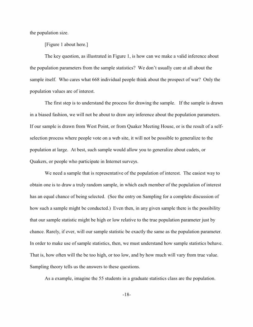
[Figure 1 about here.]

The key question, as illustrated in Figure 1, is how can we make a valid inference about

the population parameters from the sample statistics? We don’t usually care at all about the

sample itself. Who cares what 668 individual people think about the prospect of war? Only the

population values are of interest.

The first step is to understand the process for drawing the sample. If the sample is drawn

in a biased fashion, we will not be about to draw any inference about the population parameters.

If our sample is drawn from West Point, or from Quaker Meeting House, or is the result of a self-

selection process where people vote on a web site, it will not be possible to generalize to the

population at large. At best, such sample would allow you to generalize about cadets, or

Quakers, or people who participate in Internet surveys.

We need a sample that is representative of the population of interest. The easiest way to

obtain one is to draw a truly random sample, in which each member of the population of interest

has an equal chance of being selected. (See the entry on Sampling for a complete discussion of

how such a sample might be conducted.) Even then, in any given sample there is the possibility

that our sample statistic might be high or low relative to the true population parameter just by

chance. Rarely, if ever, will our sample statistic be exactly the same as the population parameter.

In order to make use of sample statistics, then, we must understand how sample statistics behave.

That is, how often will the be too high, or too low, and by how much will vary from true value.

Sampling theory tells us the answers to these questions.

As a example, imagine the 55 students in a graduate statistics class are the population.

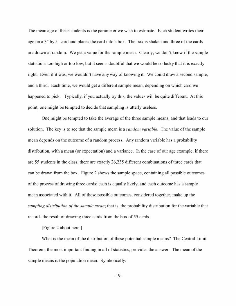
-19-

The mean age of these students is the parameter we wish to estimate. Each student writes their

age on a 3" by 5" card and places the card into a box. The box is shaken and three of the cards

are drawn at random. We get a value for the sample mean. Clearly, we don’t know if the sample

statistic is too high or too low, but it seems doubtful that we would be so lucky that it is exactly

right. Even if it was, we wouldn’t have any way of knowing it. We could draw a second sample,

and a third. Each time, we would get a different sample mean, depending on which card we

happened to pick. Typically, if you actually try this, the values will be quite different. At this

point, one might be tempted to decide that sampling is utterly useless.

One might be tempted to take the average of the three sample means, and that leads to our

solution. The key is to see that the sample mean is a random variable. The value of the sample

mean depends on the outcome of a random process. Any random variable has a probability

distribution, with a mean (or expectation) and a variance. In the case of our age example, if there

are 55 students in the class, there are exactly 26,235 different combinations of three cards that

can be drawn from the box. Figure 2 shows the sample space, containing all possible outcomes

of the process of drawing three cards; each is equally likely, and each outcome has a sample

mean associated with it. All of these possible outcomes, considered together, make up the

sampling distribution of the sample mean; that is, the probability distribution for the variable that

records the result of drawing three cards from the box of 55 cards.

[Figure 2 about here.]

What is the mean of the distribution of these potential sample means? The Central Limit

Theorem, the most important finding in all of statistics, provides the answer. The mean of the

sample means is the population mean. Symbolically:

-20-

On the one hand, this is very good news. It says that any given sample mean is not biased. The

expectation for a sample mean is equal to the population parameter we are trying to estimate. On

the other hand, this information is not very helpful. The expectation of the sample mean just tells

us what we would expect in the long run if we could kept drawing sample repeatedly. In most

cases, however, we only get to draw one sample. Our one sample could still be high or low, and

so it seems we have not made any progress.

But we have. The sample mean, as a random variable, also has a variance and a standard

deviation. The Central Limit Theorem also tells us that:

This formula tells us that the degree of variation in sample means is determined by only two

factors, the underlying variability in the population, and the sample size. If there is little

variability in the population itself, there will be little variation in the sample means. If all the

students in the class are 24 years of age, each and every sample drawn from that population will

also be 24; if there is great variability in the ages of the students, there is also the potential for

great variability in the sample means. But that variability will unambiguously decline as the

sample size, n, grows larger. The standard deviation of the sample means is referred to as the

standard error of the mean. Note that the size of the population does not matter, just the size of

the sample. Thus, a sample size of 668 out of 100,000 yields estimates that are just as accurate

as samples of 668 out of 290 million.

-21-

The Central Limit Theorem provides one additional piece of information about the

distribution of the sample mean. If the population values of the variable X are normally

distributed, then the distribution of sample mean of X will also be normally distributed. More

importantly, even if X is not at all normally distributed, the distribution of the sample mean of X

will approach normality as the sample size approaches infinity. As a matter of fact, even with

relatively small samples of 30 observations, the distribution of the sample mean will approximate

normality, regardless of the underlying distribution of the variable itself.

We now have a complete description of the probability distribution of the sample mean,

also known as the sampling distribution of the mean. The sampling distribution is a highly

abstract concept, yet it is the key to understanding how we can drawn a valid inference about a

population of 290 million from a sample of only 668 persons. The central point to understand is

that the unit of analysis in the sampling distribution is the sample mean. In contrast, the unit of

analysis in the population and the sample is, in this case, people. The sample mean, assuming a

normally distributed population or a large enough sample, is a normally distributed random

variable.

This property of the sample mean enables us to make fairly specific statements about how

often and by how much it will deviate from its expectation, the true population mean. In general,

a normally distributed random variable will take on values within 1.96 standard deviations of the

variable’s mean about 95 percent of the time. (See the entry for Normal Distribution.) In this

case, we are talking about the sample mean, and the standard deviation of sample means is called

the standard error and is given by equation X, and the mean of the sample means is equal to the

underlying population mean.

-22-

Concretely, the normality of the sampling distribution implies that the probability is 0.95

that a randomly chosen sample will have a sample mean that is within 1.96 standard errors of the

true population mean, assuming the conditions for normality of the sampling distribution are met.

And therefore it follows, as night follows day, that the probability must also be 0.95 that the

true population mean is within two standard errors of whatever sample mean we obtain in a given

sample. Mathematically,

implies that

.

One can derive the second formula from the first mathematically, but the logic is clear: if New

York is 100 miles from Philadelphia, then Philadelphia is 100 miles from New York. If there is a

95 percent probability that the sample mean will be within 1.96 standard errors of the true mean,

then the probability that the true mean is 1.96 standard errors of the sample mean is also 95

percent. The first statement tells us about the behavior of the sample mean as a random variable,

but the latter statement provides us with truly useful information: an interval that includes the

unknown population mean 95 percent of the time. This interval is known as the 95 percent

confidence interval for th mean. Other levels of confidence, e.g. 90 percent and 99 percent may

be selected, in which case the 1.96 must be replaced by a different figure, but 95 percent is by far

the most common choice.

A simpler and more common way of writing the 95 percent confidence interval is to

-23-

provide the point estimate (PE) plus or minus the margin of error (ME), as follows:

The point estimate is simply is simply an unbiased sample statistic, and is our best guess about

the true value of the population parameter. The margin of error is based on the distribution of the

sample statistic, which in this example is a normal. Thus, distributional parameter of 1.96, based

on the normal distribution, and the standard error of the estimator generate the margin of error.

One practical issue needs to be resolved. If the mean of the variable X is unknown, than

it is quite likely that the standard deviation of X is also unknown. Thus, we will need to use the

sample standard deviation, s, in place of the population standard deviation, F, in calculating the

confidence interval. Of course, s is also a random variable, and introduces more uncertainty into

our estimation, and therefore our confidence interval will have to be wider. In place of the

normal distribution threshold of 1.96, we will have to use the corresponding threshold from the t

distribution with same degrees of freedom as were used to calculate s – that is, the sample size

minus one. One can think of this as the penalty we have to pay for being uncertain about the

variance of the underlying variable. The fewer the degrees of freedom, the larger the penalty.

For samples much greater than 30, the Student’s t distribution effectively converges to the

normal and the penalty becomes inconsequential.

[Figure 3 about here.]

Figure 3 summarizes the theory of sampling. We have a population with unknown

parameters. We draw a single sample, and calculate the relevant sample statistics. The

theoretical construct of the sampling distribution, based on the Central Limit Theorem, is what

-24-

enables us to make an inference back to the population. For any estimator of any population

parameter, the sample by itself is useless and would not support inferences about the population.

Only by reference to the sampling distribution of estimator can valid inferences be drawn. Thus,

we need to understand the properties of the sampling distribution of the statistic of interest. The

following section describes some of the most commonly encountered statistics and their

sampling distributions.

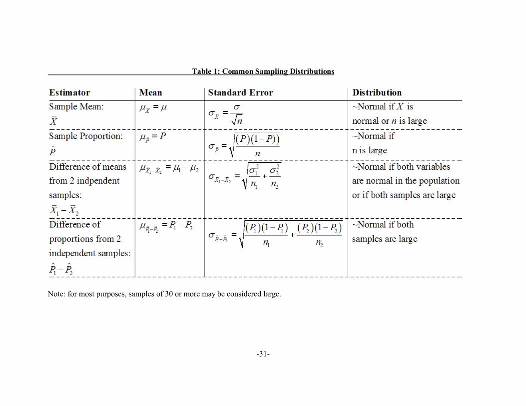
B. Common Sampling Distributions

All statistics are estimators of population parameters that are calculated from samples,

and therefore all statistics are random variables. Table 1 below describes the essential features of

the sampling distributions of the most common estimators.

[Table 1 about here.]

The expected value, variance, and shape of some estimators is not known. For example,

there is no known analytic solution for the sampling distribution of a difference of two medians.

Yet it is easy to imagine a scenario in which this would be the preferred estimator, for example in

an experimental trial where there are small samples, many extreme values drawn from an

unknown but highly skewed distribution, and unreliable measurement instruments. The viral

load of AIDS patients in a clinical trial is one example.

In such cases, it would seem that no valid inference can be drawn from a sample, because

the sampling distribution is not known. When the parameters of a sampling distribution are not

known analytically, they may be estimated empirically using a technique known as bootstrapping

(Efron 1979). In this procedure, numerous samples are drawn with replacement from the original

-25-

sample, and the measured variability of the statistic of interest across these samples is used as the

estimate of the statistic’s standard error.

III. Cautions and Conclusions.

Statistics, as a discipline, is a bit schizophrenic. On the one hand, given a specific set of

observations, there are precise formulas for calculating the mean, variance, skewness, kurtosis,

and a hundred other descriptive statistics. On the other hand, the best that inferential statistics

can tell you is that the right answer is probably between two numbers, but then again, maybe not.

Even after the best statistical analysis, we do not know the truth with complete precision. We

remain in a state of ignorance, but with an important difference: we have sharply reduced the

degree of our ignorance. Rather than not knowing a figure at all, such as the poverty rate for the

United States, we can say that we are 95 percent confident that in 2002 the poverty was between

10.1 and 10.5 percent.

A number of caveats are in order. The arguments above assume random, or at least

unbiased samples. The margin of error, based on sampling theory, applies only to the random

errors generated by the sampling process, and not the systematic errors that may be caused by bad

sampling procedures or poor measurement of the variables. If the variables are poorly conceived

or inaccurately measured, the maxim “garbage in, garbage out”will apply. Moreover, there is a

tendency, in the pursuit of mathematical rigor, to ignore variables which can not be easily

quantified, leading to the problem of omitted variable bias.

In a sense, statistics have the potential to be the refutation of the philosophical doctrine of

solipsism, which says that, because the data of our senses can be misleading, we have no true

-26-

knowledge of the outside world. With statistics, we can compile evidence that is sufficient to

convince us of a conclusion about reality with a reasonable degree of confidence. Statistics is a

tool, and an extremely valuable one at that. But it is neither the beginning nor the end of

scientific inquiry.

FURTHER READING.

Blalock, H. M., Jr. (1972). Social Statistics. New York: McGraw-Hill.

Everitt, Brian S. (1998). The Cambridge Dictionary of Statistics. Cambridge: Cambridge, U.K.:University Press.

Fruend, John E. And Ronald Walpole (1992). Mathematical Statistics, 5th ed.. EnglewoodCliffs, New Jersey: Prentice-Hall.

Hacking, Ian (1975). The Emergence of Probability: A Philosophical Study of Early Ideas aboutProbability, Induction, and Statistical Inference. London: Cambridge University Press.

Kotz, Samuel, Normal L. Johnson, and Campbell Read, eds. (1989). Encyclopedia of SocialStatistics. New York: Wiley.

Krippendorf, K. (1986). Information Theory. Newbury Park, Calif.: Sage Publications.

Pearson, E. S. And M. G. Kendall, eds. (1970). Studies in the History of Statistics andProbability. Darien, Conn.: Hafner Publishing Company.

Stigler, Stephen M. (1986). The History of Statistics: the Measurement of Uncertainty Before1900. Cambridge, Mass.: Harvard University Press.

Tukey, John W. (1977). Exploratory Data Analysis. Reading, Mass.: Addison-Wesley.

Vogt, W. Paul (1993). Dictionary of Statistics and Methodology: A Nontechnical Guide for theSocial Sciences. Newbury Park, Calif.: Sage Publications.

-27-

Weisberg, Herbert F. (1992). Central Tendency and Variability. Newbury Park, Calif.: SagePublications.

-28-

Figu

re 1

: Th

e Inferen

ce Prob

lem.

-29-

Figure 2: Samples of 3 Drawn from a Class of 55

-30-

Figure 3: Sampling Theory

-31-

Table 1: Common Sampling Distributions

Note: for most purposes, samples of 30 or more may be considered large.