NASA Reference Publication 1327 Lawrence Livermore Nationai Laboratory Report UCRL-ID-113855 1993 National Aermauhcs and Space Administration Oftice of Management Scienwic and Technical Infmatim Rogram 1993 Description and Use of LSODE, the Livermore Solver for Ordinary Differential Equations , Krishnan Radhakrishnan Sverdrup Technology, Inc. Uwis Research Center Group Alan C. Hindmarsh Lawrence Livermore National Laboratory Livermore, CA

Welcome message from author
This document is posted to help you gain knowledge. Please leave a comment to let me know what you think about it! Share it to your friends and learn new things together.
Transcript
NASA Reference Publication 1327
Lawrence Livermore Nationai Laboratory Report UCRL-ID-113855
1993
National Aermauhcs and Space Administration Oftice of Management Scienwic and Technical Infmatim Rogram 1993
Description and Use of LSODE, the Livermore Solver for Ordinary Differential Equations
, Krishnan Radhakrishnan Sverdrup Technology, Inc. Uwis Research Center Group
Alan C. Hindmarsh Lawrence Livermore National Laboratory Livermore, CA

Preface This document provides a comprehensive description of LSODE, a solver for
initial value problems in ordinary differential equation systems. It is intended to bring together numerous materials documenting various aspects of LSODE, including technical reports on the methods used, published papers on LSODE, usage documentation contained within the LSODE source, and unpublished notes on algorithmic details.
The three central chapters-n methods, code description, and code usage-are largely independent. Thus, for example, we intend that readers who are familiar with the solution methods and interested in how they are implemented in LSODE can read the Introduction and then chapter 3, Description of Code, without reading chapter 2, Description and Implementation of Methods. Similarly, those interested solely in how to use the code need read only the Introduction and then chapter 4, Description of Code Usage. In this case chapter 5, Example Problem, which illustrates code usage by means of a simple, stiff chemical kinetics problem, supplements chapter 4 and may be of further assistance.
Although this document is intended mainly for users of LSODE, it can be used as supplementary reading material for graduate and advanced undergraduate courses on numerical methods. Engineers and scientists who use numerical solution methods for ordinary differential equations may also benefit from this document.
... Ill

Contents ListofFigures ................................................. ix
ListofTables ................................................... ,
Chapter1 Introduction .......................................... 1
Chapter 2 Description and Implementation of Methods ............... 7 2.1 Linear Multistep Methods .................................... 7 2.2 Corrector Iteration Methods ................................... 9
2.2.2 Newton-Raphson Iteration ............................ 13 2.2.3 Jacobi-Newton Iteration .............................. 15 2.2.4 Unified Formulation ................................. 15
2.3 MatrixFormulation ........................................ 17 2.4 Nordsieck's History Matrix ................................. -20 2.5 Local Truncation Error Estimate and Control .................... 28 2.6 Corrector Convergence Test and Control ........................ 32 2.7 Step Size and Method Order Selection and Change ............... 33 2.8 Interpolation at Output Stations ............................... 36 2.9 Starting Procedure ......................................... 39
2.2.1 Functional Iteration .................................. 11
Chapter 3 Description of Code ................................... 41 3.1 Integration and Corrector Iteration Methods ..................... 41
3.3 Internal Communication .................................... 46 3.4 Special Features ........................................... 46
3.4.1 -Initial Step Size Calculation ........................... 57 3.4.2 Switching Methods .................................. 64
Excessive Accuracy Specification Test ................... 64 3.4.4 Calculation of Method Coefficients .................... -65 3.4.5 Numerical Jacobians ................................. 66 3.4.6 Solution of Linear System of Equations .................. 69 3.4.7 Jacobian Matrix Update .............................. 70
3.2 Codestructure ............................................ 42
3.4.3
V
~~~
Contents
3.4.8 Corrector Iteration Convergence and Corrective Actions ..... 70 3.4.9 Local Truncation Error Test and Corrective Actions . . . . . . . . 71 3.4.10 Step Size and Method Order Selection . . . . . . . . . . . . . . . . . . . 72
3.5 Error Messages ............................................ 74
Chapter 4 Description of Code Usage ............................. 75 4.1 Code Installation .......................................... 75
4.1.1 BLOCK DATA Variables ............................. 75 4.1.2 Modifying Subroutine XERRWV ....................... 76
4.3 User-Supplied Subroutine for Derivatives (F) .................... 83 4.4 User-Supplied Subroutine for Analytical Jacobian (JAC) ........... 84 4.5 Detailed Usage Notes ...................................... -85
4.5.1 Normal Usage Mode ................................. 86 4.5.2 Use of Other Options ................................ 86 4.5.3 Dimensioning Variables .............................. 86 4.5.4 Decreasing the Number of Differential Equations (NEQ) .... 87 4.5.5 Specification of Output Station (TOUT) . . . . . . . . . . . . . . . . . 87 4.5.6 Specification of Critical Stopping Point (TCRTT) . . . . . . . . . . 88 4.5.7 Selection of Local Error Control Parameters
(ITOL, RTOL, and ATOL) ............................ 88 4.5.8 Selection of Integration and Corrector Iteration
Methods(MF) ...................................... 89 4.5.9 Switching Integration and Corrector Iteration Methods . . . . . . 91
4.6 Optional Input . . . . . . . . . . . . . . . . . . . . . . . . . . . . . . . . . . . . . . . . . . . . 91 4.6.1 Initial Step Size (HO) . . . . . . . . . . . . . . . . . . . . . . . . . . . . . . . . 92 4.6.2 Maximum Step Size (HMAX) ......................... 92 4.6.3 Maximum Method Order (MAXORD) . . . . . . . . . . . . . . . . . . . 92
4.7 Optional Output ........................................... 92 4.8 Other Routines ............................................ 93
4.8.1 Interpolation Routine (Subroutine INTDY) . . . . . . . . . . . . . . . 93 4.8.2 Using Restart Capability (Subroutine SRCOM) ............ 94 4.8.3 Error Message Control (Subroutines XSETF and
XSETUN) ......................................... 95 4.9 Optionally Replaceable Routines .............................. 95
4.9.2 Vector-Norm Computation (Function VNORM) ........... 97 4.10 Overlay Situation ......................................... 98 4.11 Troubleshooting .......................................... 98
Chapter 5 Example Problem .................................... 101 5.1 Description of Problem .................................... 101 5.2 Coding Required To Use LSODE ............................ 102
5.2.1 General ........................................... 102
4.2 Callsequence ............................................ 76
4.9.1 Setting Error Weights (Subroutine EWSET) .............. 95
vi
5.2.2 Selection of Parameters . 5.3 Computed Results ..........
Chapter 6 Code Availability ......
References ....................
.............
.............
.............
.............
......
......
......
......
...
...
...
...
Contents
........ 102
........ 104
........ 105
........ 107
vii

.
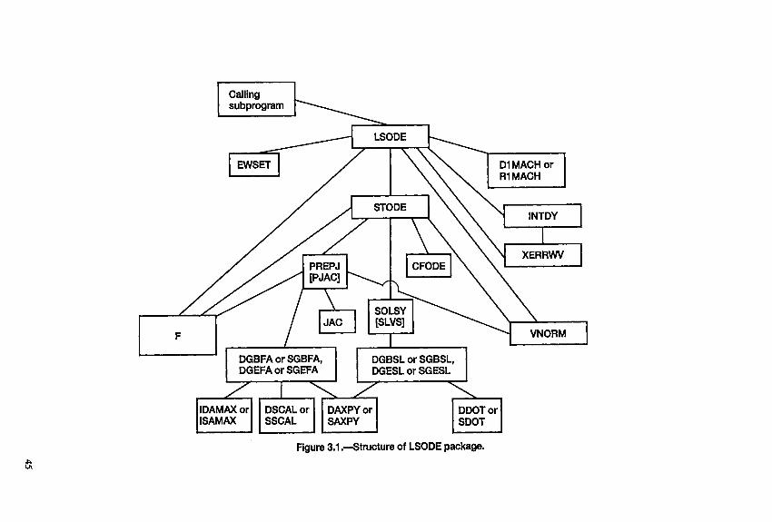
List of Figures Figu.re 3.1.-Structure of MODE package .........................
Figure 3.2.-Howchart of subroutine LSODE .......................
Figure 33.-Nowchart of subroutine STODE .......................
Figure 5.L-Listing of hUIN program for example problem ...........
Figure 5.2.-Listing of subroutine (FEX) that computes derivatives for example problem ............................................
Figure 53.-Listing of subroutine (JEX) that computes analytical Jacobian matrix for example problem ...................................
Figure 5.4.4utput from program for example problem ...............
.45
.59
.61
103
103
104
104
ix

List of Tables Table 2.1,Method coefficients for Adams-Moulton method in normal
form of orders 1 to 12 . . . . . . . . . . . . . . . . . . . . . . . . . . . . . . . . . . . - . . . . . -25
Table 23.-Method coefficients for backward differentiation formula method in normal form of orders 1 to 6 . . . . . . . . . . . . . . . . . . . . . . . . . . . .26
Table 3.1.4ummary of integration methods included in LSODE and corresponding values of METH, the first decimal digit of MF . . . . . . .42
Table 3.2.--Corrector iteration techniques available in LSODE and corresponding values of MITER, the second decimal digit of MF . . . . . . .32
Table 3.3.-Description of subprograms used in LSODE . . . . . . . . . . . . . . . .44
Table 3A.-Routines with common blocks, subprograms, and calling subprograms in double-precision version of LSODE . . . . . . . . . . . . . . . . . .47
Table 3.5-Routines with common blocks, subprograms, and calling subprograms in single-precision version of LSODE . . . . . . . . . . . . . . . . . .48
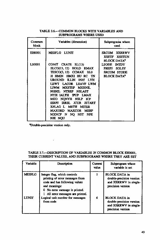
Table 3.6.-Common blocks with variables and subprograms where used . . .49
Table 3.7.-Description of variables in common block EHOOO1, their current values, and subprograms where they are set . . . . . . . . . . . . . . . . . . .49
Table 3.8.-Description of variables in common block LSOOO1, their current values, if any, and subprograms where they are set orcomputed ................................................. 50
Table 39.-Length LENWM of array WM in table 3.8 for iteration techniques included in code . . . . . . . . . . . . . . . . . . . . . . . . . . . . . . . . . . . . .55
Table 4.1.-Values of ITASK used in LSODE and their meanings . . . . . . . . .77
Table 4.2.-Values of ITOL used in LSODE and their meanings . . . . . . . . . .78
Table 4.3.-Values of ISTATE that can be used on input to LSODE and their meanings . . . . . . . . . . . . . . . . . . . . . . . . . . . . . . . . . . . . . . . . . . . .79
Table 4.4.-Values of ISTATE returned by LSODE and their meanings . . . .79
xi
List of Tables
Table 4.5.-Values of IOPT that can be used on input to LSODE andtheirmeanings ............................................ 80
Table 4.6.-Optional input parameters that can be set by user and their locations, meanings, and default values ........................... .80
Table 4.7.-Optional output parameters returned by LSODE and their locationsandmeanings ......................................... 82
Table 4.8.-Useful informational quantities regarding integration that can be obtained from array RWORK and their names and locations . . . . . .82
Table 4.9.-Minimum length required by real work array RWORK (Le., minimum LRW) for each MF ................................... .83
Table 4.10.-Minimum length required by integer work array WORK I (Le., minimum LIW) for each MITER ............................ .83
xii
Chapter 1 Introduction
This report describes a FORTRAN subroutine package, LSODE, the Livermore Solver for Ordinary Differential Equations, written by Hindmarsh (refs. 1 and 2), and the methods included therein for the numerical solution of the initial value problem for a system of first-order ordinary differential equations (ODE'S). Such a problem can be written as
1 ~$5,~) = yo = Given,
where - y, -0 Y , - 9, and f are column vectors with N (2 1) components and 5 is the independent variable, for example, time or distance. In component form equa- tion (1. l) may be written as
i = 1, ..., N. (12)
I y j ( e 0 ) = yj,o = Given
The initial value problem is to find the solution function y at one or more values of 5 in a prescribed integration interval [ h b n d ] , where thi initial value of 1, yo, at 6 = is given. The endpoint, Lnd, may not be known in advance as, for example, when asymptotic values of y as 5 + 00 are required.
Initial value, first-order ODE'S arise in many fields, such as chemical kinetics, biology, electric network analysis, and control theory. It is assumed that the
1
1. Introduction
problem is well posed and possesses a solution that is unique in the interval of interest. Solution existence and uniqueness are guaranteed if, in the region of interest, f is defined and continuous and for any two vectors y and y* in that region there exists a positive constant 9 such that (refs. 3 and 4)-
-
which is known as a Lipschitz condition. Here 11-11 denotes a vector norm (e.g., ref. 5), and the constant 9 is known as a Lipschitz constant off with respect to y .
The right-hand side f of the ODE system must be a function of y and 5 only. Tt cannot therefore involve y at previous 5 values, as in delay or retGded ODE’s or integrodifferential equations. It cannot also involve random variables, as in stochastic differential equations. A second- or higher-order ODE system must be reduced to a first-order ODE system.
The solution methods included in LSODE replace the ODE’s with difference equations and then solve them step by step. Starting with the initial conditions at 50, approximations L(= YiPm i = 1, ...,N) to the exact solution y(Cn) [= y,(cn), i = 1, ...,Nl of the ODE’s are generated at the discrete mesh points& (n = 1,2, ...), which are themselves determined by the package. The spacing between any two mesh points is called the step size or step length and is denoted by h,, where
An important feature of LSODE is its capability of solving ‘‘stiff’ ODE problems. For reasons discussed by Shampine (ref. 6 ) stiffness does not have a simple definition involving only the mathematical problem, equation (1.1). However, Shampine and Gear (ref. 7) discuss some fundamental issues related to stiffness and how it arises. An approximate description of a stiff ODE system is that it contains both very rapidly and very slowly decaying terms. Also, a characteristic of such a system is that the NxN Jacobian matrix J (= af/dy), with element .Il, defined as
-
J-. = ah/ayj. i , j = 1 ,..., N , I/
has eigenvalues {hi} with real parts that are predominantly negative and also vary widely in magnitude. Now the solution varies locally as a linear combination of the exponentials { ecRe(’,)}, which all decay if all Re& ) < 0, where Re&) is the real part of h,. Hence for sufficiently large 5 (> l/maxlRe(hi)l, where the bars 1.1 denote absolute value), the terms with the largest Re&) will have decayed to insignificantly small levels while others are still active, and the problem would be classified as stiff. If, on the other hand, the integration interval is limited to l/maxlRe(hi)l, the problem would not be considered stiff.
2
1. Introduction
In this discussion we have assumed that all eigenvalues have negative real parts. Some of the Re&) may be nonnegative, so that some solution components are nondecaying. However, the problem is still considered stiff if no eigenvalue has a real part that is both positive and large in magnitude and at least one eigenvalue has a real part that is both negative and large in magnitude (ref. 7). Because the {hi} are, in general, not constant, the property of stiffness is local in that a problem may be stiff in some intervals and not in others. It is also relative in the sense that one problem may be more stiff than another. A quantitative measure of stiffness is usually given by the stifmess ratio max[-Re(hi)]/min [-Re&)]. This measure is also local for the reason given previously. Another standard measure for stiffness is the quantity max[-Re(&)l[&,d - 501. This measure is more relevant than the previous one when Isend - $01 is a better indicator of the average “resolution scale” for the problem than l/min[-Re(hi)]. (In some cases min[-Re(hi)] = 0.)
The difficulty with stiff problems is the prohibitive amounts of computer time required for their solution by classical ODE solution methods, such as the popular explicit Runge-Kutta and Adams methods. The reason is the excessively small step sizes that these methods must use to satisfy stability requirements. Because of the approximate nature of the solutions generated by numerical integration methods, errors are inevitably introduced at every step. For a numerical method to be stable, errors introduced at any one step should not grow unbounded as the calculation proceeds. To maintain numerical stability, classical ODE solution methods must use small step sizes of order l/max[-Re(hi)] even after the rapidly decaying components have decreased to negligible levels. Examples of the step size pattern used by an explicit Runge-Kutta method in solving stiff ODE problems arising in combustion chemistry are given in references 8 and 9. Now, the size of the integration interval for the evolution of the slowly varying components is of order l/min[-Re(hi)]. Consequently, the number of steps required by classical methods to solve the problem is of order max[-Re(&)]/min[-Re(&)], which is very large for stiff ODE’S.
For stiff problems the LSODE package uses the backward differentiation formula (BDF) method (e.g., ref. lo), which is among the most popular currently used for such problems (ref. 11). The BDF method possesses the property of stiff stability (ref. 10) and therefore does not suffer from the stability step size constraint once the rapid components have decayed to negligible levels. Throughout the integration the step size is limited only by accuracy requirements imposed on the numerical solution. Accuracy of a numerical method refers to the magnitude of the error introduced in a single step or, more precisely, the local truncation or discretization error. The local truncation error & at & is the difference between the computed approximation and the exact solution, with both starting the integration at the previous mesh point tn-1 and using the exact solution y (&-I) as the initial value. The local truncation error on any step is therefore &e error incurred on that step under the assumption of no past errors (e.g., ref. 12).
The accuracy of a numerical method is usually measured by its order. A method is said to be of order 4 if the local truncation error varies as hi+’. More
3
1. Introduction
precisely, a numerical method is of order 4 if there are quantities C and h, (> 0) such that (refs. 3 and 13)
for all 0 < h, I h,,
where is an N-dimensional column vector containing the absolute values of the dj,n (i = 1, ...,N). The coefficient vectorc may depend on the function defining the ODE and the total integration interval, but it should be independent of the step size h, (ref. 13). Accuracy of a numerical method refers to the smallness of the error introduced in a single step; stability refers to whether or not this error grows in subsequent steps (ref. 7).
To satisfy accuracy requirements, the BDF method may have to use small step sizes of order l/max(Re I&l) in regions where the most rapid exponentials are active. However, outside these regions, which are usually small relative to the total integration interval, larger step sizes may be used.
The LSODE package also includes the implicit Adams method (e.g., refs. 4 and IO), which is well suited for nonstiff problems. Both integration methods belong to the family of linear multistep methods. As implemented in LSODE these methods allow both the step size and the method order to vary (from I to 12 for the Adams method and from 1 to 5 for the BDF method) throughout the problem. The capability of dynamically varying the step size and the method order is very important to the efficient use of linear multistep methods (ref. 14).
The LSODE package consists of 2 1 subprograms and a BLOCK DATA module. The package has been designed to be used as a single unit, and in normal circumstances the user needs to communicate with only a single subprogram, also called LSODE for convenience. LSODE is based on, and in many ways resembles, the package GEAR (ref. 1 3 , which, in turn, is based on the code DIFSUB, written by Gear (refs. 10 and 16). All three codes use integration methods that are based on a constant step size but are implemented in a manner that allows for the step size to be dynamically varied throughout the problem. There are, however, many differences between GEAR and LSODE, with the following important improvements in LSODE over GEAR: (1) its user interface is much more flexible; (2) it is more extensively modularized; and ( 3 ) it uses dynamic storage allocation, different linear algebra modules, and a wider range of error types (ref. 17). Most significantly, LSODE has been designed to virtually eliminate the need for user adjustments or modifications to the package before it can be used effectively. For example, the use of dynamic storage allocation means that the required total storage is specified once in the user-supplied subprogram that communicates with LSODE; there is no need to adjust any dimension declarations in the package. This feature, besides making the code easy to use, minimizes the total storage requirements; only the storage required for the user's problem needs to be allocated and not that called for by a code using default values for parameters, such as the total number of ODES, for example. The many different capabilities of the code can be exploited quite simply by setting values for appropriate
4
1. Introduction parameters in the user’s subprogram. Not requiring any adjustments to the code eliminates the user’s need to become familiar with the inner workings of the code, which can therefore be used as a “black box,” and, more importantly, eliminates the possibility of errors being introduced into the modified version.
The remainder of this report is organized as follows: In chapter 2 we describe the numerical integration methods used in LSODE and how they are implemented in practice. The material presented in this chapter is based on, and closely follows, the developments by Gear (refs. 10 and 18 to 20) and Hindmarsh (refs. 1, 2, 15, 21, and 22). Chapter 3 describes the features and layout of the LSODE package. In chapter 4 we provide a detailed guide to its usage, including possible user modifications. The use of the code is illustrated by means of a simple test problem in chapter 5. We conclude this report with a brief discussion on code availability in chapter 6.
5

Chapter 2 Description and Implementa- tion of Methods 2.1 Linear Multistep Methods
The numerical methods included in the packaged code LSODE generate approximate solutions X to the ordinary differential equations (ODE'S) at discrete points & (n = 1,2, ...). Assuming that the approximate solutions L+ have been computed at the mesh points 5n-j (j = lY2, ...), these methods advance the solution to the current value & of the independent variable by using linear multistep
. formulas of the type
j=l j = O
where the current approximate solution vector 41, consists of N components,
and the superscript T indicates transpose. In equation (2. l), fn-i [= is the approximation to the exact derivative vector at cn+, y(&+) [= f( y(cn+))], where for notational convenience the 5 argument off has b&n droppedrthe coefficients {a,} and {pi} and the integers K1 and K2 are associated with a particular methd, and h, (= tn - &-I) is the step size to be attempted on the current step [5n-1,&]. The method is called linear because the {Yj} and { f i } occur linearly. It is called multistep because it uses information from several previous mesh points. The number max(K1, K2) gives the number of previous values involved.
The values K1 = 1 and K2 = q - 1 produce the popular implicit Adams, or Adams-Moulton (AM), method of order q:
7
(2.6a)
(2.6b)
2.2 Corrector Iteration Methods methods are given by Gear (ref. 10) for q 5 6 . In equation (2.5), although the subscript n has been attached to the step size h, indicating that h, is the step size to be attempted on the current step, the methods used in LSODE are based on a constant h. When the step size is changed, the data at the new spacing required to continue the integration are obtained by interpolating from the data at the original spacing. Solution methods and codes that are based on variable step size have also been developed (refs. 17,23, and 24) but are not considered in the present work.
2.2 Corrector Iteration Methods
If Po = 0, the methods are called explicit because they involve only the known values {&} and {&+}, and equation (2.1) is easy to solve. If, however, Po # 0, the methods are called implicit and, in general, solution of equation (2.1) is expensive. For both methods, equations (2.3) and (2.4), Po is positive for each q and because f is, in general, nonlinear, some type of iterative procedure is needed to solve equation (2.5). Nevertheless, implicit methods are preferred because they are more stable, and hence can use much larger step sizes, than explicit methods and are also more accurate for the same order and step size (refs. 4, 10, and 12). Explicit methods are used as predictors, which generate an initial guess for X. The implicit method corrects the initial guess iteratively and provides a reasonable approximation to the solution of equation (2.5).
The predictor-corrector process for advancing the numerical solution to & therefore consists of first generating a predicted value, denoted by a'], and then correcting this initial estimate by iterating equation (2.5) to convergence. That is, starting with the initial guess ~ ' 1 , approximations am] (m = 1,2, ...m are generated (by using one of the techniques discussed below) until the magnitude of the difference in two successive approximations approaches zero within a specified accuracy. The quantity am] is the approximation obtained on the mth iteration, the integer M is the number of iterations required for convergence, and we accept g[MJ as an approximation to the exact solution y at Cn and therefore denote it by X although, in general, it does not satisfy equagon (2.5) exactly.
At each iteration m the quantity h,Zp1, which is defined here, is computed from ~ " ' 1 by the relation
Now, as discussed by Hindmarsh (ref. 21) and shown later in this section, if am] converges as m -+ 00, the limit, that is, , must be a solution of
equation (2.5) and Sz1 converges to f , [= €&)I, the approximation to - y(en).
Em1 lim Y n m-w-
9
2. Description and implementation of Methods
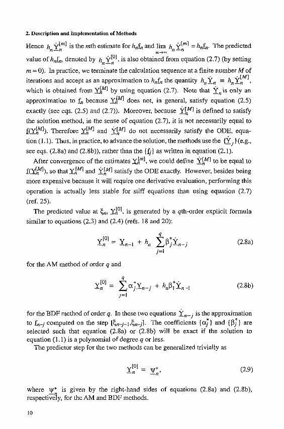
Hence h y[" l is the mth estimate for hnfn and lim h y["] = h,&. The predicted
value of h&, denoted by h y lo1 , is also obtained from equation (2.7) (by setting
m = 0). In practice, we terminate the calculation sequence at a finite number M of [MI iterations and accept as an approximation to h& the quantity hn%n hn%, ,
which is obtained from dw by using equation (2.7). Note that %,is only an approximation to fn because Gw does not, in general, satisfy equation (2.5) exactly (see eqs. (2.5) and (2.7)). Moreover, because TLM] is defined to satisfy the solution method, in the sense of equation (2.7), it is not necessarily equal to f(Y[nMl). Therefore 4lff"l and %LMl do not necessarily satisfy the ODE, equa- tion (1. l). Thus, in practice, to advance the solution, the methods use the {% } (e.g., see eqs. (2.8a) and (2.8b)), rather than the { f j } as written in equation (2.1),
After convergence of the estimates $"'I, we could define TiM] to be equal to f ( ~ ! ) , so that G'l and 45fYIl satisfy the ODE exactly. However, besides being more expensive because it will require one derivative evaluation, performing this operation is actually less stable for stiff equations than using equation (2.7) (ref. 25).
The predicted value at cn, do], is generated by a qth-order explicit formula similar to equations (2.3) and (2.4) (refs. 18 and 20):
m-00 n-n n -n
n -n
j=1
for the AM method of order q and
(2.8a)
(2.8b)
for the BDF method of order q. In these two equations ' n - j is the approximation to fn-j computed on the step [E,n-j-l,cn-j]. The coefficients {a;} and {p;} are selected such that equation (2.8a) or (2.8b) will be exact if the solution to equation (1.1) is a polynomial of degree q or less.
The predictor step for the two methods can be generalized trivially as
(2.9)
where y ~ * is given by the right-hand sides of equations (2.8a) and (2.8b), respectiGIy, for the Ah4 and BDF methods.
10
2.2. Corrector Iteration Methods
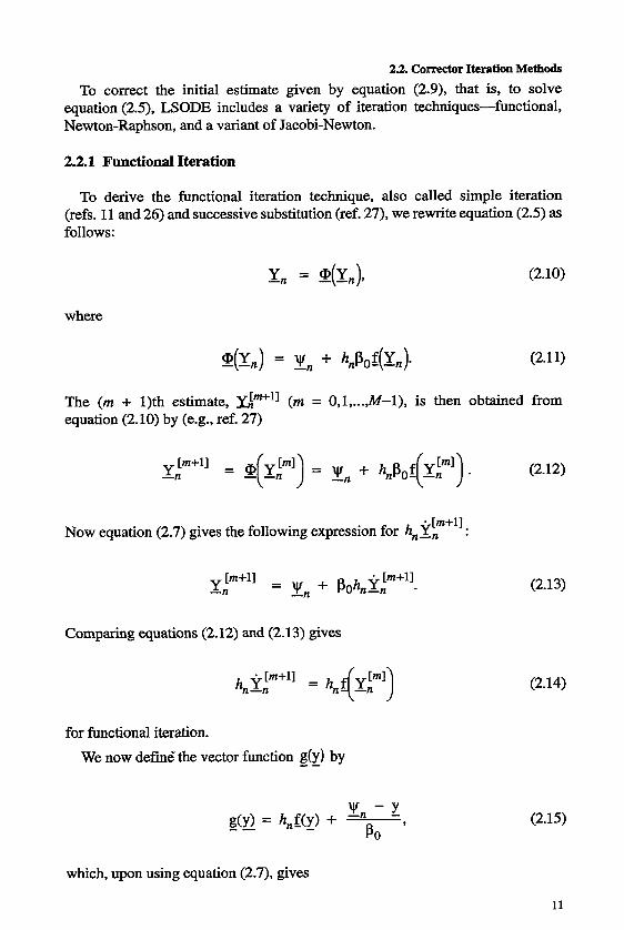
To correct the initial estimate given by equation (2.9), that is, to solve equation (2.5), LSODE includes a variety of iteration techniques-functional, Newton-Raphson, and a variant of Jacobi-Newton.
2.2.1 Functional Iteration
To derive the functional iteration technique, also called simple iteration (refs. 11 and 26) and successive substitution (ref. 27), we rewrite equation (2.5) as follows:
where
The (m + 1)th estimate, Gm+ll (m = O , l , ..., M-1), is then obtained from equation (2.10) by (e.g., ref. 27)
. [m+l] Now equation (2.7) gives the following expression for hnyn
Comparing equations (2.12) and (2.13) gives
for functional iteration.
We now define’ the vector function g(y) - - by
(2.12)
(2.13)
(2.14)
(2.15)
which, upon using equation (2.7), gives
11
2. Description and Implementation of Methods
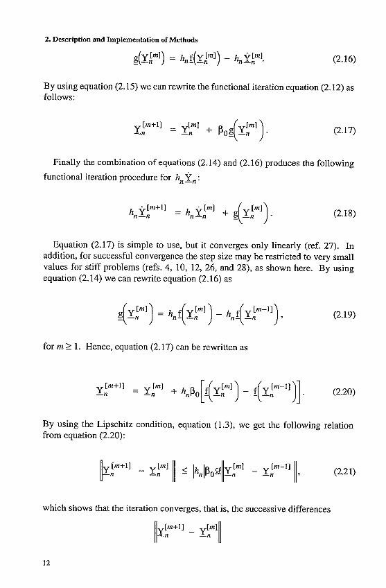
(2.16)
By using equation (2.15) we can rewrite the functional iteration equation (2.12) as follows:
Finally the combination of equations (2.14) and (2.16) produces the following
functional iteration procedure for hnk, :
Equation (2.17) is simple to use, but it converges only linearly (ref. 27). In addition, for successful convergence the step size may be restricted to very small values for stiff problems (refs. 4, 10, 12, 26, and 28), as shown here. By using equation (2.14) we can rewrite equation (2.16) as
for m 2 1. Hence, equation (2.17) can be rewritten as
By using the Lipschitz condition, equation (1.3), we get the following relation from equation (2.20):
which shows that the iteration converges, that is, the successive differences
12
2.2. Corrector Iteration Methods
decrease, only if
(h,(Poa 1- (222)
Now stiff problems are characterized by, and often referred to as systems with, large Lipschitz constants (e.g., refs. 4, 12, and 26), and so equation (2.22) restricts the step size to very small values. Indeed, the restriction imposed by this inequality on h, is exactly of the same form as that imposed by stability requirements on classical methods, such as the explicit Runge-Kutta method (refs. 4 and 26). For this reason, when functional iteration is used, the integration method is usually said to be explicit even though it is implicit (ref. 17).
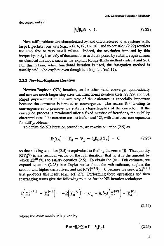
2.2.2 Newton-Raphson Iteration
Newton-Raphson (NR) iteration, on the other hand, converges quadratically and can use much larger step sizes than functional iteration (refs. 27,29, and 30). Rapid improvement in the accuracy of the estimates is especially important because the corrector is iterated to convergence. The reason for iterating to convergence is to preserve the stability characteristics of the corrector. If the correction process is terminated after a fixed number of iterations, the stability characteristics of the corrector are lost (refs. 4 and 12), with disastrous consequences for stiff problems.
To derive the NR iteration procedure, we rewrite equation (2.5) as
(2.23)
so that solving equation (2.5) is equivalent to finding the zero of E. The quantity B a r n $ is the residual vector on the mth iteration; that is, it is the amount by which ~ m l fails to satisfy equation (2.5). To obtain the (m + 1)th estimate, we expand equation (2.23) in a Taylor series about the mth estimate, neglect the second and higher derivatives, and set Bdm+’]) = 0 because we seek a ~ m + ’ l that produces this result (e.g., ref. 27). Performing these operations and then rearranging terms give the following relation for the NR iteration technique:
(2.24)
where the NXN matrix P is given by
13
2. Description and Implementation of Methods
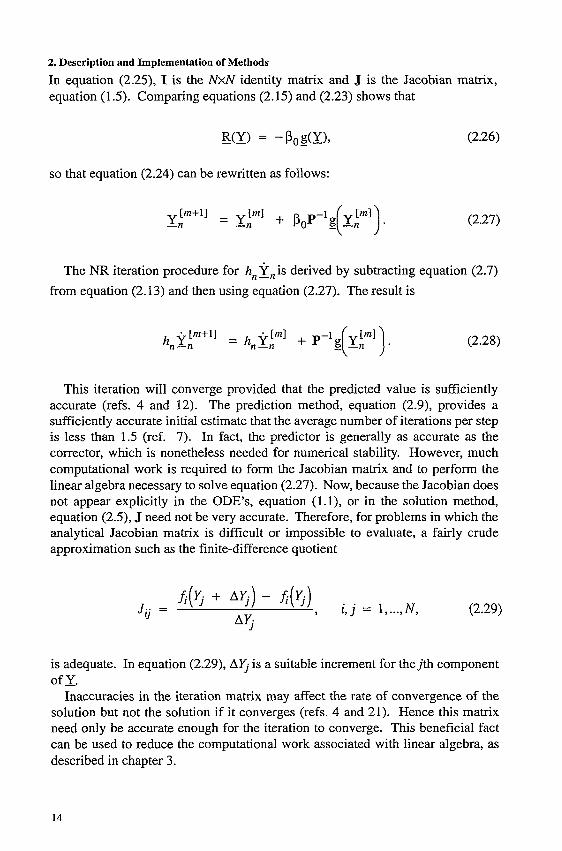
In equation (2.25), I is the NxN identity matrix and J is the Jacobian matrix, equation (1 3. Comparing equations (2.15) and (2.23) shows that
so that equation (2.24) can be rewritten as follows:
(2.27)
The NR iteration procedure for h,%’, is derived by subtracting equation (2.7) from equation (2.13) and then using equation (2.27). The result is
(2.28)
This iteration will converge provided that the predicted value is sufficiently accurate (refs. 4 and 12). The prediction method, equation (2.9), provides a sufficiently accurate initial estimate that the average number of iterations per step is less than 1.5 (ref. 7). In fact, the predictor is generally as accurate as the corrector, which is nonetheless needed for numerical stability. However, much computational work is required to form the Jacobian matrix and to perform the linear algebra necessary to solve equation (2.27). Now, because the Jacobian does not appear explicitly in the ODE’S, equation (1. I), or in the solution method, equation (2.5), J need not be very accurate. Therefore, for problems in which the analytical Jacobian matrix is difficult or impossible to evaluate, a fairly crude approximation such as the finite-difference quotient
is adequate. In equation (2.29), A 5 is a suitable increment for thejth component
Inaccuracies in the iteration matrix may affect the rate of convergence of the solution but not the solution if it converges (refs. 4 and 21). Hence this matrix need only be accurate enough for the iteration to converge. This beneficial fact can be used to reduce the computational work associated with linear algebra, as described in chapter 3.
of y.
14
2.2. Corrector Iteration Methods 2.2.3 Jacobi-Newton Iteration
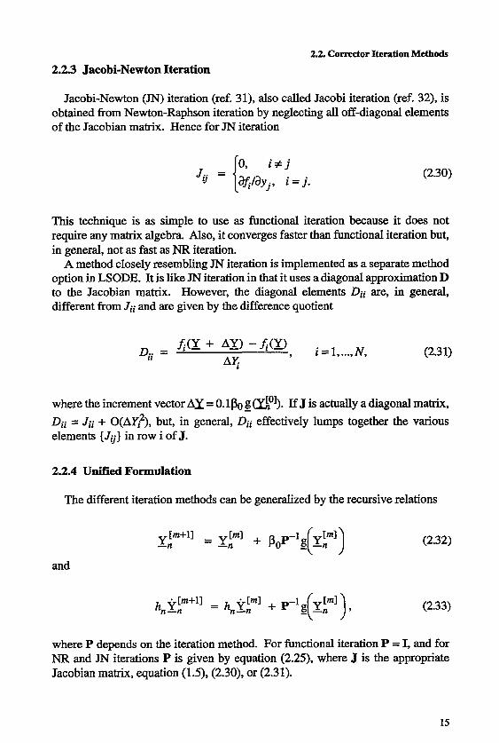
Jacobi-Newton (JN) iteration (ref. 31), also called Jacobi iteration (ref. 32), is obtained from Newton-Raphson iteration by neglecting all off-diagonal elements of the Jacobian matrix. Hence for JN iteration
0, i # j J. . = (2.30)
This technique is as simple to use as functional iteration because it does not require any matrix algebra. Also, it converges faster than functional iteration but, in general, not as fast as NR iteration.
A method closely resembling JN iteration is implemented as a separate method option in LSODE. It is like JN iteration in that it uses a diagonal approximation D to the Jacobian matrix. However, the diagonal elements Dii are, in general, different from Jii and are given by the difference quotient
(2.3 1)
where the increment vector A I = 0.lpo - g(YJp1). If J is actually a diagonal matrix, Dii = Jii + O(Ayi?), but, in general, Dii effectively lumps together the various elements { J g } in row i of J.
2.2.4 Unified Formulation
The different iteration methods can be generalized by the recursive relations
(2.32)
and
(2.33)
where P depends on the iteration method. For functional iteration P = I, and for NR and JN iterations P is given by equation (2.25), where J is the appropriate Jacobian matrix, equation (1.5), (2.30), or (2.31).
15
23 Matrix Formulation
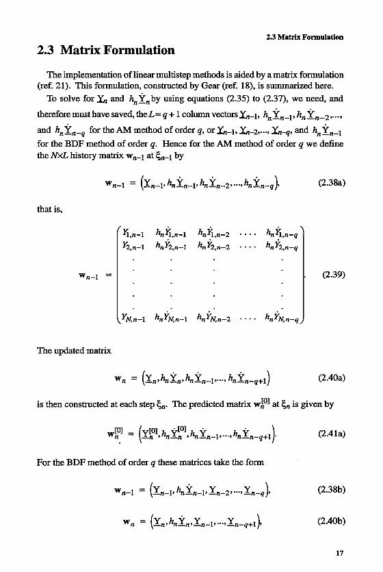
2.3 Matrix Formulation
The implementation of linear multistep methods is aided by a matrix formulation (ref. 21). This formulation, constructed by Gear (ref. 18), is summarized here.
To solve for X, and h&by using equations (2.35) to (2.37), we need, and
thereforemusthavesaved, t h e l = q + 1 columnvectorsX,-1, hngn-l, hn4n-2,..., and hngn-, for t h e m method of order q, or L-1, x-2, ..., X,*, and hngn-l for the BDF method of order 4. Hence for the AM method of order 4 we define the NxL history matrix wn-l at gn-l by
that is,
wn-l = (2.39)
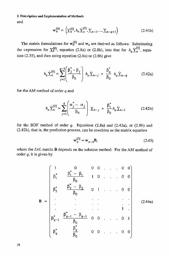
The matrix formulations for wiol and w, are derived as follows: Substituting the expression for go]. equation (2.8a) or (2.8b), into that for h,gyl, equa- tion (2.35), and then using equation (2.6a) or (2.6b) give
for the AM method of order q and
(2.42b) P i . a.- a. h n ~ ~ ] =z( ' Po '1 -n- Y J + -hnyn-l P O
J = 1
for the BDF method of order q. Equations (2.8a) and (2.42a), or (2.8b) and (2.42b), that is, the prediction process, can be rewritten as the matrix equation
w[ol n - -w,-p> (2.43)
where the LxL matrix B depends on the solution method. For the AM method of order q, it is given by
( 1 0 0 0 . . . 0 0 )
p;
p; 0 1 . . . 0 0
P ; - p l
P O
P O
1 0 . . . 0 0
B = l . . . . .
g 0 0 . 16 P O
18
23 Matrix Formulation
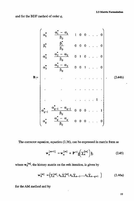
and for the BDF method of order q,
The
where
for t h e
B ,=
; corrector
wJml, the
: AM metl
* a1
P; *
a 2
a 3 *
* xq-1
aq *
* a1 - a1
PO
* a2 - a 2
P O
a 3 - a3 PO
*
* aq-1 - aq-1
P O
aq - aq
P O
*
1 0 0 . . . 0
0 0 0 . . . 0
0 1 0 . . . 0
0 0 1 . . . 0
_ - - . _ . .
. . . . . . .
. . . . . 1 .
0 0 0 . . . 1
0 0 0 . . . 0
' equation, equation (2.36), can be expressed in 1
. history matrix on the mth
iod and by
iteration, is given by
natrix
1
(2.44b)
form as
(2.45)
(2.46a)
19
for the BDF method, - k is the L-dimensional vector
and P depends on the iteration technique, as described in section 2.2.4. The matrix formulation of the methods can be summarized as follows:
Predictor:
} m=0,1, ..., M-I.
w,=w, [MI .
2.4 Nordsieck’s History Matrix
(2.46b)
(2.47) I
(2.48)
(2.49) I
(2.50)
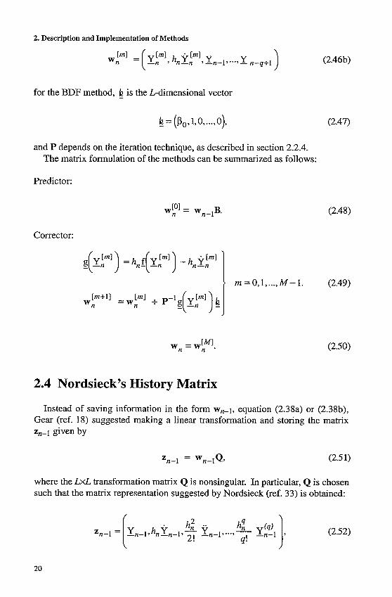
Instead of saving information in the form w,l, equation (2.38a) or (2.38b), Gear (ref. 18) suggested making a linear transformation and storing the matrix zn-l given by
where the LxL transformation matrix Q is nonsingular. In particular, Q is chosen such that the matrix representation suggested by Nordsieck (ref. 33) is obtained:
2.4 Nordsieck‘s History Matrix
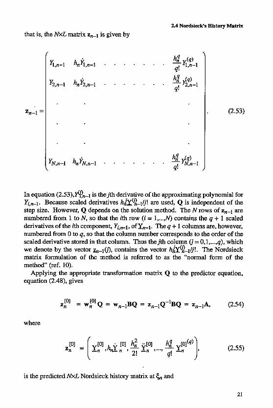
that is, the NXL matrix zn-l is given by
(2.53)
In equation (2.53),*?,-1 is thejth derivative of the approximating polynomial for Yi,*l. Because scaled derivatives h,&b?-l/j! are used, Q is independent of the step size. However, Q depends on the solution method. The N rows of zn-l are numbered from 1 to N, so that the ith row (i = 1, ...m contains the q + 1 scaled derivatives of the ith component, Yi,+l, of &-1. The q + 1 columns are, however, numbered from 0 to q, so that the column number corresponds to the order of the scaled derivative stored in that column. Thus thejth column (j = O,l, ...,q), which we denote by the vector &-lo>, contains the vector hB$-l/j!. The Nordsieck matrix formulation of the method is referred to as the “normal form of the method” (ref. 10).
Applying the appropriate transformation matrix Q to the predictor equation, equation (2.48), gives
where
(2.55)
is the predicted NxL Nordsieck history matrix at & and
21
2. Description and Implementation of Methods
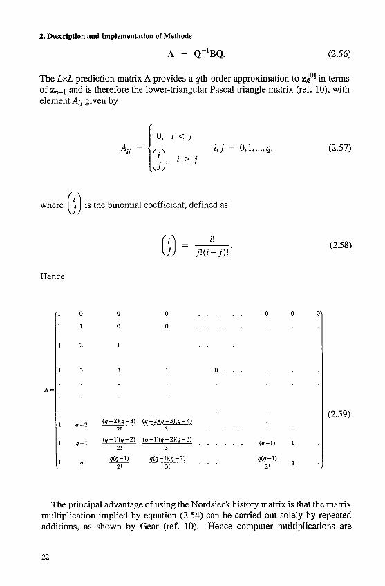
A = Q-~BQ. (2.56)
The LxL prediction matrix A provides a qth-order approximation to zhol in terms of z,-1 and is therefore the lower-triangular Pascal triangle matrix (ref. lo), with element A0 given by
l o , i < j
where ( ;) is the binomial coefficient, defined as
Hence
A :
0 0 0 . . . . . 0
1 0 0 . . . . .
2 1 . .
3 3 1 o . . .
0 0
1
9 1
(2.57)
(2.58)
(2.59)
The principal advantage of using the Nordsieck history matrix is that the matrix multiplication implied by equation (2.54) can be carried out solely by repeated additions, as shown by Gear (ref. 10). Hence computer multiplications are
2.4 Nordsieck’s History Matrix avoided, resulting in considerable savings of computational effort for large problems. Also A need not be stored and zhol overwrites z,1, thereby reducing memory requirements.
Because
(i+1) j+ l = ( j+ l ) + (;) and Aii =Ai0 = 1 for all i, the product zA is computed as follows (refs. 10 and 15):
For k=0,1, ..., 4-1, do: For j = q , q - l , ..., k + l , do:
zi,i-l tZi , i+zi , i - l , i= l , ... , N . (2.61)
In this equation the subscripts n and n-1 have been dropped because the z values do not indicate any one value of E, but represent a continuous replacement process. At the start of the calculation procedure given by equation (2.61), z = zn-l; and at the end z = zhol. The arrow “c” denotes the replacement operator, which means overwriting the contents of a computer storage location. For example,
means that zi,4 is added to zi,3 and the result replaces the contents of the location z ~ . The total number of additions required in equation (2.61) is Nq(q + 1)/2. The predictor step is a Taylor series expansion about the previous point L-1 and is independent of both the integration method and the ODE.
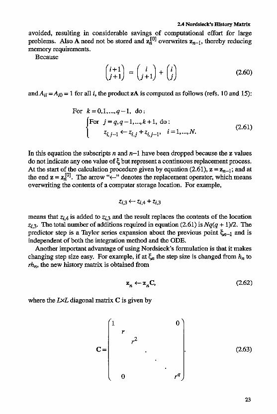
Another important advantage of using Nordsieck‘s formulation is that it makes changing step size easy. For example, if at & the step size is changed from h, to rh,, the new history matrix is obtained from
z, -,C,
where the LXL diagonal matrix C is given by
C =
1 0 r
2 r
(2.62)
(2.63)
23
2. Description and Implementation of Methods
The rescaling can be done by multiplications alone, as follows:
R = l For j = l , ...,q, do:
R t rR zi,j + Z ~ , ~ R , i = l , ..., N .
The corrector equation corresponding to equation (2.49) is given by
where ziml, the Nordsieck history matrix on the mth iteration, is given by
and
(2.64
(2.65)
(2.66)
(2.67)
is an L-dimensional vector
4 = (Q,, Q, , ..., Qq). (2.68)
For the two solution methods used in LSODE the values of 1 are derived in references 21 and 22 and reproduced in tables 2.1 and 2.2. Methods expressed in the form of equations (2.54) and (2.65) are better described as multivalue or L- value methods than multistep methods (ref. 10) because it is the number L of values saved from step to step that is significant and not the number of steps involved.
The two matrix formulations described here are related by the transformation equations (2.51), (2.54), and (2.65) and are therefore said to be equivalent (ref. 10). The equivalence means that if the step [Cn-1,&J is taken by the two methods with equivalent past values wn-l and zn-l, that is, related by equa- tion (2.51) through Q, then the resulting solutions w, and z, will also be related by equation (2.51) through Q. apart from roundoff errors (ref. 21). The transformation does not affect the stability properties or the accuracy of the
24
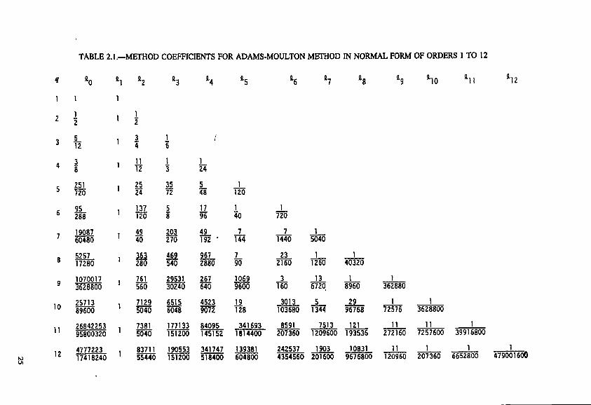
TABLE 2.1 .-METHOD COEFFICIENTS FOR ADAMS-MOULTON METHOD IN NORMAL FORM OF ORDERS 1 TO 12
4 Qo el &2 e3 '4 &5 '6 &7 '8 Q1O Q l 1 2
2 2 l 1
3 T ? l i 3
1 1 1
1 1
5 3 1 1
1
5
17 1
- 1 1 1 4 12 3 24 1 -
1 - 1 - 25 - 35 -
95 137 5 - 203 - 49 - 7 - 7 - 1 19087 49 -
5 7 2 0 24 72 48 120 251
1 - TO 720 6 - 288 l 1 2 0 5 96
7 - 1440 5040 60480 w 270 192 ' 144
1 - 1 - 23 - 469 967 - 7 17280 1 % 540 2880 90 2160 1260 40320
1 1 1070017 761 29531 267 - 1069 - _. 13 - 3628800 560 30240 640 9600 160 6720. 8960 362880
29 1 7129 6515 4523 19 - L _ 3013 5 - 25713 1 - - - l o 89600 5040 6048 9072 128
7381 177133 84095 341693 8591 7513 121 11 - 1 1 - 1 26842253 - 1 1 - 95800320 83711 190553 341747 139381 242537 1903 10831 11 - 1 1 ___ 1 4777223
3
103680 1344 96768 &6 3628800
5040 151200 145152 1814400 207360 1209600 193536 272160 7257600 39916800
h) " 17418240 ' 55440 151200 518400 604800 4354560 201600 9676800 120960 207360 6652800 479001600 VI
2. Description and Implementation of Methods
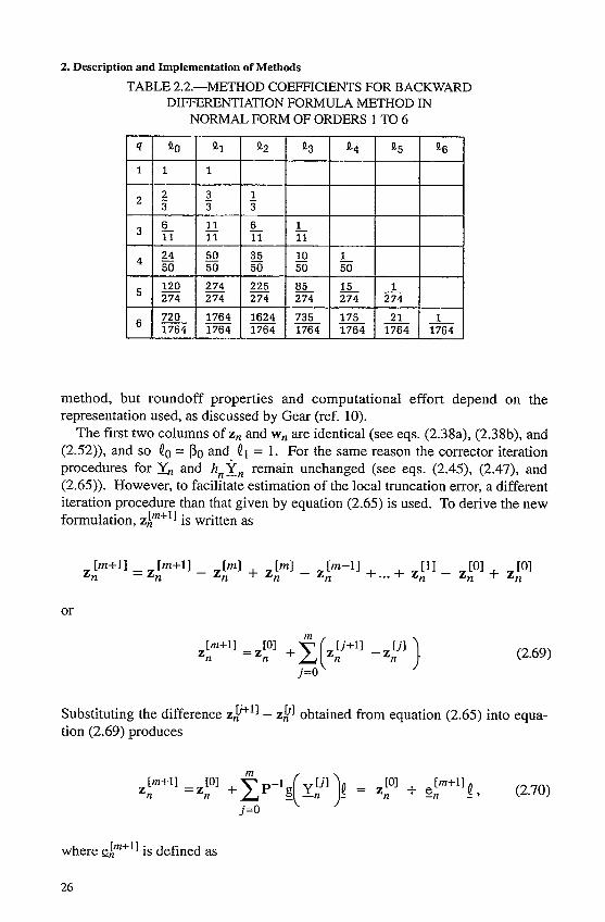
TABLE 2.2.-METHOD COEFFICIENTS FOR BACKWARD DIFFERENTIATION FORMULA METHOD IN
NORMAL FORM OF ORDERS 1 TO 6
QO
1 - z 3
6 11
24 50 120 274
720 1764
- - - - -
-
Ql - 1
3 3
11 11
50 50 274 274
- - - - - - -
1764 1764 -
Q2
- 1 3 -
6 11
35 50
274
- - - - 225
1624 - 1764
- Q3
735 1764
Q4 Q5 Q6
1 50
15 1 274 274
175 21 1 1764 1764 1764
-
- -
- - -
method, but roundoff properties and computational effort depend on the representation used, as discussed by Gear (ref. 10).
The first two columns of z, and w, are identical (see eqs. (2.38a), (2.38b), and (2.52)), and so Qo = Po and 41 = 1. For the same reason the corrector iteration procedures for & and h,%, remain unchanged (see eqs. (2.45), (2.47), and (2.65)). However, to facilitate estimation of the local truncation error, a different iteration procedure than that given by equation (2.65) is used. To derive the new formulation, zim+l1 is written as
or
(2.69)
Substituting the difference z P l 1 - zkl obtained from equation (2.65) into equa- tion (2.69) produces
\ / j=O
where c$,"'+'~ is defined as
26
2.4 Nordsieck's History Matrix
(2.71)
It is clear from this equation that
Equation (2.70) can be used to rewrite - g (arn1), equation (2.16), as follows:
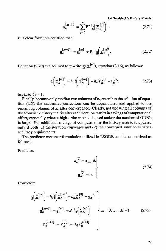
because 41 = 1. Finally, because only the first two columns of z, enter into the solution of equa-
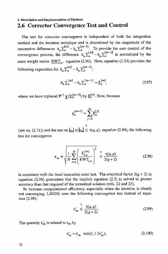
tion (2.5), the successive corrections can be accumulated and applied to the remaining columns of z, after convergence. Clearly, not updating all columns of the Nordsieck history matrix after each iteration results in savings of computational effort, especially when a high-order method is used and/or the number of ODE'S is large. For additional savings of computer time the history matrix is updated only if both (1) the iteration converges and (2) the converged solution satisfies accuracy requirements.
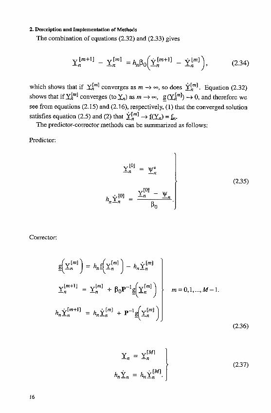
The predictor-corrector formulation utilized in LSODE can be summarized as follows:
Predictor:
Corrector:
(2.74)
27
2. Description and Implementation of Methods
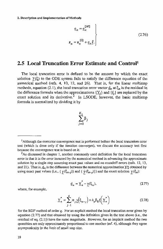
(2.76)
2.5 Local Truncation Error Estimate ancl Controll
The local truncation error is defined to be the amount by which the exact solution Y (5) to the ODE system fails to satisfy the difference equation of the numericarmethod (refs. 4, 10, 12, and 26). That is, for the linear multistep methods, equation (2. I), the local truncation error vector Si, at 5, is the residual in the difference formula when the ap roximations (Xj} and {t]} are replaced by the exact solution and its derivative! In LSODE, however, the basic multistep formula is normalized by dividing it by
j=O
'Although the corrector convergence test is performed before the local truncation error test (which is done only if the iteration converges), we discuss the accuracy test first because the convergence test is based on it.
*As discussed in chapter 1, another commonly used definition for the local truncation error is that it is the error incurred by the numerical method in advancing the approximate solution by a single step assuming exact past values and no roundoff errors (refs. 12, 13, and 21). That is, & is the difference between the numerical approximation obtained by using exact past values (Le., { y(cnj)] and [ y&-,)]) and the exact solution ~(5"): - - -
t
d" = 1" - y(c"), (2.77) where, for example,
(2.78) j=1
for the BDF method of order q. For an explicit method the local truncation error given by equation (2.77) and that obtained by using the definition given in the text above (Le., the residual of eq. (2.1)) have the same magnitude. However, for an implicit method the two quantities are only approximately proportional to one another (ref. 4), although they agree asymptotically in the limit of small step size.
28
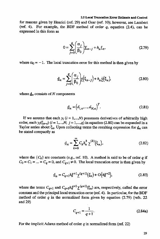
2.5 Locpl h c a t i o n Error Estimate and Control for reasons given by Henrici (ref. 29) and Gear (ref. 10); however, see Lambert (ref. 4). For example, the BDF method of order q, equation (2.4), can be expressed in this form as
where q = - 1. The local truncation error for this method is then given by
(2.79)
(2.80)
where &, consists of N components
If we assume order, each yi(E,, Taylor series ah be stated compai
that each yi (i j) (i = 1, ..., N, mt E,,. Upon c ctly as
= 1, ...m possesses derivatives of arbitrarily high j = 1, ...,q) in equation (2.80) can be expanded in a ollecting terms the resulting expression ford, can
m
(2.82) k=O
where the { c k } are constants (e.g., ref. 10). A method is said to be of order q if CO = C1= ... = C4 = 0, and Cq+l # 0. The local truncation error is then given by
Ci, = cq+1h$+1y(q+l)(5,)+ 0 ( h . 4 + 2 ) 7 (2.83)
where the terms C4+1 and Cq+1h,f+l ~(q'")(E,n) are, respectively, called the error constant and the principal local truncation error (ref. 4). In particular, for the BDF method of order q in the normalized form given by equation (2.79) (refs. 22 and 29)
1 cq+1= q+l' (2.84a)
For the implicit Adams method of order q in normalized form (ref. 22)
29
2. Description and Implementation of Methods
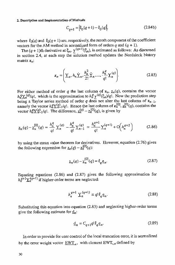
cq+l = 140 (4 + 1) - 40 (4)). (2.84b)
where Qo(q) and @o(q + 1) are, respectively, the zeroth component of the coefficient vectors for the AM method in normalized form of orders q and (q + 1).
The (q + 1)th derivative at c,, y(qf')(cn), is estimated as follows: As discussed in section 2.4, at each step the solution method updates the Nordsieck history matrix z,:
(2.85)
For either method of order q the last column of z,, zn(4), contains the vector hJL(q)/q!, which is the approximation to hz y(q)(c,)/q!. Now the prediction step being a Taylor series method of order q does not alter the last column of z,-i, namely the vector hjx($,/q!. Hence the last column of zAol, zLol(q), contains the vector h$&Ll/q!. The difference, &) - dol(q), is given by
by using the mean value theorem for derivatives. However, equation (2.76) gives the following expression for ~ ( q ) - zLol(q):
Equating equations (2.86) and (2.87) gives the following approximation for h$+'dq+') if higher-order terms are neglected:
(2.88)
Substituting this equation into equation (2.83) and neglecting higher-order terms give the following estimate for &:
In order to provide for user control of the local truncation error, it is normalized by the error weight vector E,, with element EWT,,, defined by
30
2.5 Locpl lhmcation Error Estimate and Control
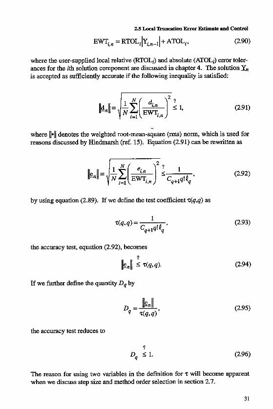
EWT~,, = RTOL~~Y~, , -~~ + ATOL,, (2.90)
where the user-supplied local relative (RTOLi) and absolute (ATOLi) error toler- ances for the ith solution component are discussed in chapter 4. The solution X is accepted as sufficiently accurate if the following inequality is satisfied:
(2.9 1)
.7
where 11.11 denotes the weighted root-mean-square (rms) norm, which is used for reasons discussed by Hindmarsh (ref. 15). Equation (2.91) can be rewritten as
by using equation (2.89). If we define the test coefficient z(4,q) as
the accuracy test, equation (2.92), becomes ?
llenll 5 z(q,q)-
If we further define the quantity D4 by
the accuracy test reduces to
? D I 1 . 4
T 'H
'he reasc rhen we
m for u discuss
sing step
two size
variables in and method
the definition for order selection in
z will become section 2.7.
(2.92)
(2.93)
(2.94)
(2.95)
(2.96)
apparent
31
(2.100)
2.7 Step Size and Method Order Selection and Change
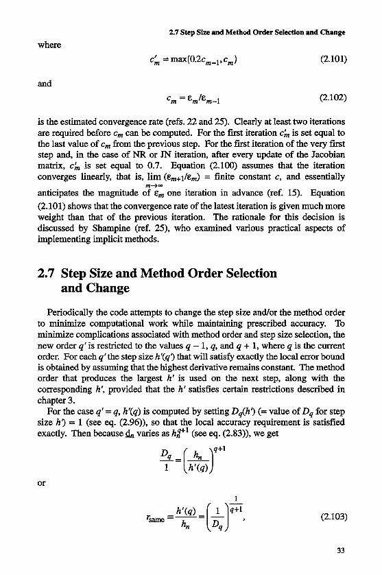
where ck = max(0.2~,-~, cm) (2.101)
and
is the estimated convergence rate (refs. 22 and 25). Clearly at least two iterations are required before cm can be computed. For the first iteration c& is set equal to the last value of c, from the previous step. For the first iteration of the very first step and, in the case of NR or JN iteration, after every update of the Jacobian matrix, c& is set equal to 0.7. Equation (2.100) assumes that the iteration converges linearly, that is, lim (E,+#,) = finite constant cy and essentially
m-w- anticipates the magnitude of em one iteration in advance (ref. 15). Equation (2.101) shows that the convergence rate of the latest iteration is given much more weight than that of the previous iteration. The rationale for this decision is discussed by Shampine (ref. 25), who examined various practical aspects of implementing implicit methods.
2.7 Step Size and Method Order Selection and Change
Periodically the code attempts to change the step size and/or the method order to minimize computational work while maintaining prescribed accuracy. To minimize complications associated with method order and step size selection, the new order 4' is restricted to the values 4 - 1, 4, and 4 + 1, where 4 is the current order. For each q'the step size h'(q') that will satisfy exactly the local error bound is obtained by assuming that the highest derivative remains constant. The method order that produces the largest h' is used on the next step, along with the corresponding h', provided that the h' satisfies certain restrictions described in chapter 3.
For the case 4' = 4, h'(q) is computed by setting D&') (= value of D, for step size h') = 1 (see eq. (2.96)), so that the local accuracy requirement is satisfied exactly. Then because d, varies as h,4'l (see eq. (2.83)), we get
or
1 , ,-
(2.103)
33
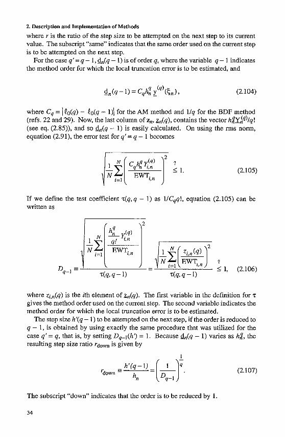
2. Description and Implementation of Methods
where r is the ratio of the step size to be attempted on the next step to its current value. The subscript “same” indicates that the same order used on the current step is to be attempted on the next step.
For the case q‘ = 4 - 1, &(q - 1) is of order q, where the variable 4 - 1 indicates the method order for which the local truncation error is to be estimated, and
where Cq = I Qo(q) - Qo(q - 1)1 for the AM method and l/q for the BDF method (refs. 22 and 29). Now, the last column of z,, z,(q), contains the vector h$&q)/q! (see eq. (2.85)), and so &(q - 1) is easily calculated. On using the rms norm, equation (2.91), the error test for 4’ = q - 1 becomes
(2.105)
If we define the test coefficient ~ ( q , q - 1) as l/Cqq!, equation (2.105) can be written as
1 I 1, (2.106)
where zi,Jq) is the ith element of ~,(q). The first variable in the definition for ‘I: gives the method order used on the current step. The second variable indicates the method order for which the local truncation error is to be estimated.
The step size h’(4 - 1) to be attempted on the next step, if the order is reduced to 4 - 1, is obtained by using exactly the same procedure that was utilized for the case q‘ = 4, that is, by setting Dq-l(h’) = 1. Because &(q - 1) varies as h i , the resulting step size ratio ‘down is given by
1
The subscript “down” indicates that the order is to be reduced by 1.
34
(2.107)
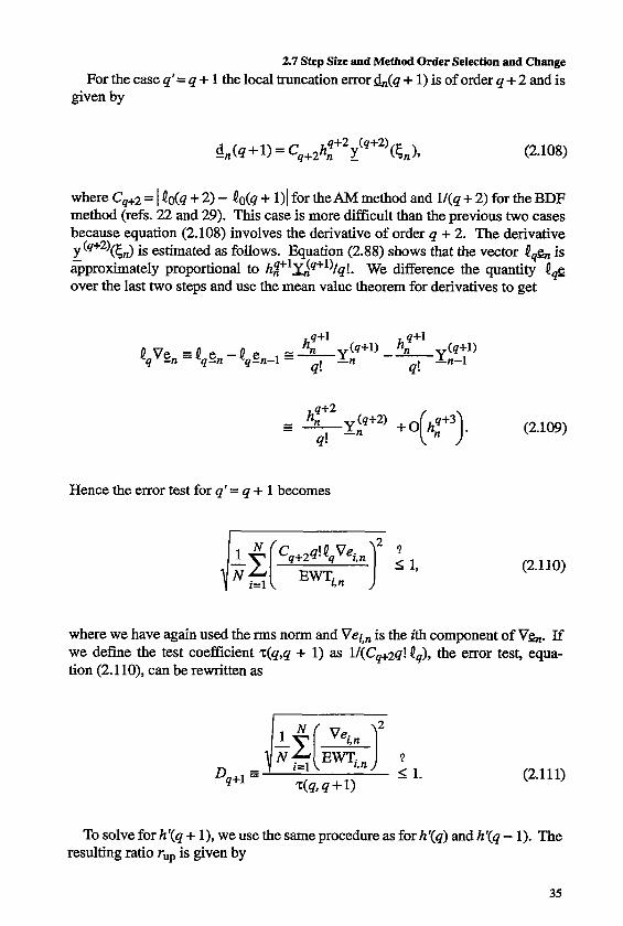
2.7 Step Size and Method Order Selection and Change For the case q'= q + 1 the local truncation error &(q + 1) is of order q + 2 and is
given by
(2.108)
where Cq+2 = I to(4 + 2) - to(q + 1)1 for t h e m method and l/(q + 2) for the BDF method (refs. 22 and 29). This case is more difficult than the previous two cases because equation (2.108) involves the derivative of order q + 2. The derivative
is estimated as follows. Equation (2.88) shows that the vector 4,& is @proximately proportional to h$+lGq+')/q!. We difference the quantity tqg over the last two steps and use the mean value theorem for derivatives to get
Hence the error test for 4'= q + 1 becomes
(2.1 10)
where we have again used the ms norm and Vei,, is the ith component of V&. If we define the test coefficient z(q,q + 1) as 1/(Ce2q!tq), the error test, qua - tion (2. l lo), can be rewritten as
(2.1 11)
To solve for h'(q + l), we use the same procedure as for h'(q) and h'(q - 1). The resulting ratio rUp is given by
35
(2.1 12)
2.8 Interpolation at Output Stations
therefore important that in implementing the solution method provision be made for the efficient computation of the solution at the required output stations. Moreover, the procedure used for these computations should not adversely affect the efficiency of the integration beyond the output station. Such a situation arises, for example, if the method has to adjust the step size to “hit” the output station exactly. Because the Nordsieck history array is used to store past history information, the solution can be generated at the output stations quite easily, as described next.
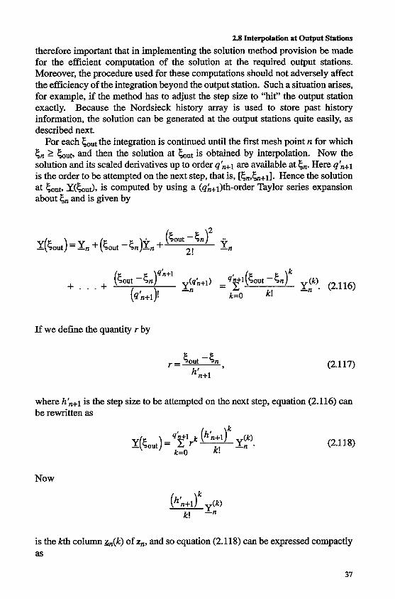
For each E,,,,,, the integration is continued until the first mesh point n for which 2 Lut, and then the solution at LUt is obtained by interpolation. Now the
solution and its scaled derivatives up to order 4;t+1 are available at cn. Here q;t+1 is the order to be attempted on the next step, that is, [Cn,&+l]. Hence the solution at SOUt, X(LuJ, is computed by using a (q;+l)th-order Taylor series expansion about cn and is given by
If we define the quantity r by
(2.1 17)
where h;t+1 is the step size to be attempted on the next step, equation (2.116) can be rewritten as
(2.118)
Now
is the kth column ~ ( k ) of z,, and so equation (2.11 8) can be expressed compactly as
37
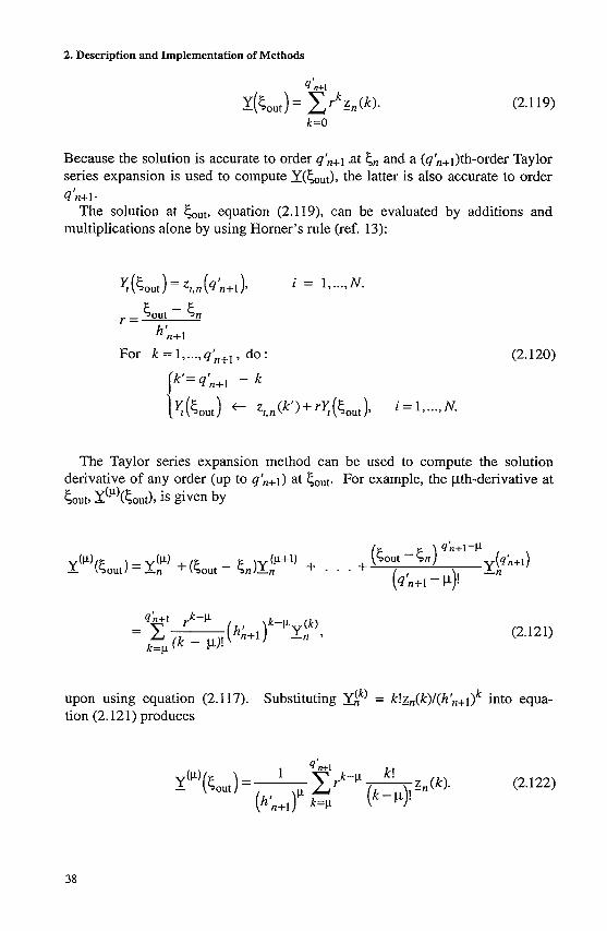
(2.120)
2.9 Starting Procedure
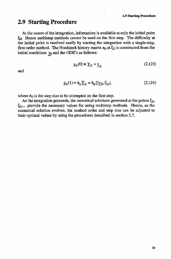
2.9 Starting Procedure
At the outset of the integration, information is available at only the initial point 50. Hence multistep methods cannot be used on the first step. The difficulty at the initial point is resolved easily by starting the integration with a single-step, first-order method. The Nordsieck history matrix zo at 50 is constructed fiom the initial conditions yo and the ODE'S as follows: -
(2.123)
where ho is the step size to be attempted on the first step. As the integration proceeds, the numerical solutions generated at the points 51,
52, ... provide the necessary values for using multistep methods. Hence, as the numerical solution evolves, the method order and step size can be adjusted to their optimal values by using the procedures described in section 2.7.
39

Chapter 3 Description of Code 3.1 Integration and Corrector Iteration Methods
The packaged code LSODE has been designed for the numerical solution of a system of first-order ordinary differential equations (ODE’S) given the initial values. It includes a variable-step, variable-order Adams-Moulton (AM) method (suitable for nonstiff problems) of orders 1 to 12 and a variable-step, variable- order backward differentiation formula PDF) method (suitable for stiff problems) of orders 1 to 5. However, the code contains an option whereby for either method a smaller maximum method order than the default value can be specified.
Irrespective of the solution method the code starts the integration with a first- order method and, as the integration proceeds, automatically adjusts the method order (and the step size) for optimal efficiency while satisfying prescribed accuracy requirements. Both integration methods are step-by-step methods. That is, starting with the known initial condition ~ ( 5 0 ) at 50, where y is the vector of dependent variables, 5 is the independent ;&able, and 50 is ig initial value, the methods generate numerical approximations Y, to the exact solution y (E,n> at the discrete points Gn (n = 1,2, ...) until the end of the integration interval% reached. At each step [&-&,J both methods employ a predictor-corrector scheme, wherein an initial guess for the solution is first obtained and then the guess is improved upon by iteration. That is, startin with an initial guess, denoted by ~ ‘ 1 , successively improved estimatesdmy(m = 1, ...,M) are generated until the iteration converges, that is, further iteration produces little or no change in the solution. Here &ml is the approximation computed on the mth iteration, and M is the number of iterations required for convergence.
A standard explicit predictor formula-a Taylor series expansion method devised by Nordsieck (ref. 33)-is used to generate the initial estimate for the solution. A range of iteration techniques for correcting this estimate is included in LSODE. Both the basic integration method and the corrector iteration procedure are identified by means of the method flag h4F. By definition, h4F has the two decimal digits METH and MITER, and
41
3. Description of Code
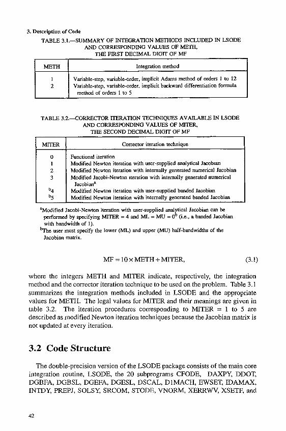
TABLE 3.1.-SUMMARY OF INTEGRATION METHODS INCLUDED IN LSODE AND CORRESWNDING VALUES OF METH,
THE FIRST DECIMAL DIGIT OF MF
METH Integration method
I 2
Variable-step, variable-order. implicit Adams method of orders 1 to 12 Variable-step, variable-order, implicit bxkward differentiation formula
method of orders 1 to 5
TABLE 3.2.4ORRECTOR ITERATION TECHNIQUES AVAILABLE IN LSODE AND CORRESPONDING VALUES OF MITER, THE SECOND DECIMAL DIGlT OF MF
0 1 2 3
b4 b5
~~~~
Corrector iteration tcchniaue
Functional iteration Modified Newton iteration with user-supplied analytical Jrroblan Modified Newton iteration with internally generated numerical Jacobian Modified Jacobi-Newton iteration with internally generated numerical
Modified Newton iteration with user-supplied banded Jacobian Modified Newton iteration with internally generated banded Jacobian
Jacobiana
aModified Jacobi-Newton iteration with user-supplied analytical Jacobian can be. performed by specifying MITER = 4 and ML = Mu = Ob (Le., a banded Jacobian with bandwidth of I).
Jacobian matrix. %e user must specify the lower (ML) and upper (MU) half-bandwidths of the
MF=lOxMETH+MITER, (3.1
where the integers METH and MITER indicate, respectively, the integration method and the corrector iteration technique to be used on the problem. Table 3.1 summarizes the integration methods included in LSODE and the appropriate values for METH. The legal values for MITER and their meanings are given in table 3.2. The iteration procedures corresponding to MITER = 1 to 5 are described as modified Newton iteration techniques because the Jacobian matrix is not updated at every iteration.
3.2 Code Structure
The double-precision version of the LSODE package consists of the main core integration routine, LSODE, the 20 subprograms CFODE, DAXPY, DDOT, DGBFA, DGBSL, DGEFA, DGESL, DSCAL, DlMACH, EWSET, IDAMAX, INTDY, PREPJ, SOLSY, SRCOM, STODE, VNORM, XElZRWV, XSETF, and
42
3.2 Code Structure
XSETUN, and a BLOCK DATA module for loading some variables. The single- precision version contains the main routine, LSODE, and the 20 subprograms CFODE, EWSET, INTDY, ISAMAX, PREPJ, RlMACH, SAXPY, SDOT, SGBFA, SGBSL, SGEFA, SGESL, SOLSY, SRCOM, SSCAL, STODE, WORh4, XERRWV, XSETF, and XSETUN. The subprograms DDOT, DlMACH, IDAMAX, ISAMAX, RlMACH, SDOT, and WORM are function routines-all the others are subroutines. The subroutine XERRWV is machine dependent. In addition to these routines the following intrinsic and external routines are used: DABS, DFLOAT, DMAX1, DMIN1, DSIGN, and DSQRT by the double-precision version; ABS, AMAX1, AMIN1, FLOAT, SIGN, and SQRT by the single-precision version; and MAXO, M I N O , MOD, and WRITE by both versions.
Table 3.3 lists the subprograms in the order that they appear in the code and briefly describes each subprogram. Among these, the routines DAXPY, DDOT, DGBFA, DGBSL, DGEFA, DGESL, DSCAL, IDAMAX, ISAMAX, SAXPY, SDOT, SGBFA, SGBSL, SGEFA, SGESL, and SSCAL were taken from the LINPACK collection (ref. 34). The subroutines XERRW, XSETF, and XSETUN, as used in LSODE, constitute a simplified version of the SLATEC error-handling package (ref. 35).
The structure of the LSODE package is illustrated in figure 3.1, wherein a line connecting two routines indicates that the lower routine is called by the upper one. For subprograms that have different names in the different versions of the code, both names are given, with the double-precision version name listed first. Also, the names in brackets are dummy procedure names, which are used internally and passed in call sequences. The routine F is a user-supplied subroutine that computes the derivatives dyi/& (i = 1, ...,N), where yi is the ith component of y and Nis the number of ODE’S. Finally, the user-supplied subroutine JAC computes the analytical Jacobian matrix J (= af/ay), where f = dy/&.
The code has been arranged as much as possibl~in a “modular” fashion, with different subprograms performing different tasks. Hehce the number of subprograms is fairly large. However, this feature aids in both understanding and, if necessary, modifying the code. To enhance the user’s understanding of the code, it contains many comment statements, which are gfouped together in blocks and describe both d e task to be performed next and theprocedure to be used. In addition, each subprogram includes detailed explanatory notes, which describe the function of the subprogram, the means of communication (i.e., call sequence andor common blocks), and the input and output variables.
Each subprogram contains data type declarations for all variables in the routine. Such declarations are useful for debugging and provide a list of all variables that occur in a routine. This list is useful in overlay situations. For each data type the variables are usually listed in the following order: variables that are passed in the call sequence, variables appearing in common blocks, and local variables, in either alphabetical order or the order in which they appear in the call sequence and the common blocks.
43
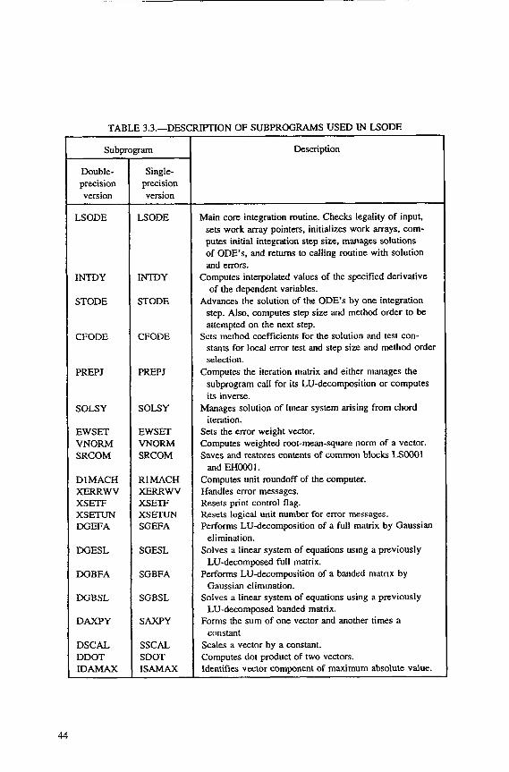
TABLE 3.3.-DESCRTPTION OF SUBPROGRAMS USED IN LSODE
I Subprogram
Double- precision version
LSODE
INTDY
STODE
CFODE
PREPJ
I SOLSY
EWSET VNORM SRCOM
DlMACH XERRWV x s m XSETUN DGEFA
DGESL
DGBFA
DGBSL
DAXPY
DSCAL DDOT IDAMAX
Single- precision version
LSODE
tNmY
STODE
CFODE
PREPJ
SOLSY
EWSET VNORM SRCOM
R1 MACH XERRWV XSETF XSETUN SGEFA
SGESL
SGBFA
SGBSL
SAXPY
SSCAL SDOT ISAMAX
Description
Main core integration routine. Checks legality of input, sets work array pointers. initializes work arrays. com- putes initial integration step size, manages solutions of ODE's. and returns to calling routine with solution and errors.
Computes interpolated values of the specified derivative of the dependent variables.
Advances the solution of the ODE's by one integration step. Also, compute.. step size and method order to be attempted on the next step.
stants for local error test and step size and method order selection.
subprogram call for its LU-decomposition or computes its inverse.
iteration.
Sets method coefficients for the solution and test con-
Computes the iteration matrix and either manages the
Manages solution of linear system arising from chord
Sets the error weight vector. Computes weighted root-mean-square norm of a vector. Savcs and restores contents of common blocks LSooOl
Computes unit roundoff of the computer. Handles error messages. Resets print control flag. Resets logical unit number for error messages. Performs LUdecomposition of a full matrix by Gaussian
Solves a linear system of equations using a previously
Performs LUdecomposition of a banded matnx by
Solves a linear system of equations using a previously
Forms the sum of one vector and another times a
Scales a vector by a constant. Computes dot product of two vectors. Identifies vector component of maximum absolute value.
and EHOOO 1.
elimination.
LU-decomposed full matrix.
Gaussian elimination.
LU-decomposed banded matrix.
constant
Calling
IDAMAX or ISAMAX
EWSET
DSCAL or DAXPY or DDOT or SSCAL SAXPY SDOT
3. Description of Code
3.3 Internal Communication
Communication between different subprograms is accomplished by means of both call sequences and the two common blocks EHOOOl and LSOOO1. The reason for using common blocks is to avoid lengthy call sequences, which can significantly deteriorate the efficiency of the program. However, common blocks are not used for variables whose dimensions are not known at compilation time. Instead, to both eliminate user adjustments to the code and minimize total storage requirements, dynamic dimensioning is used for such variables.
The common blocks, if any, used by each subprogram are given in tables 3.4 and 3.5 for the double- and single-precision versions, respectively. These tables also list all routines called and referenced (e.g., an external function) by each subprogram. Also, to facilitate use of LSODE in overlay situations, all routines that call and reference each subprogram are listed. Finally, for each subprogram the two tables give dummy procedure names (which are passed in call sequences and therefore have to be declared external in each calling and called subprogram) in brackets.
The variables included in the two common blocks and their dimensions, if different from unity, are listed in table 3.6. The common blocks contain variables that are (1) local to any routine but whose values must be preserved between calls to that routine and (2) communicated between routines. The structure of the block LSOOOl is as follows: All real variables are listed first, then all integer variables. Within each group the variables are arranged in the following order: (1) those local to subroutine LSODE, (2) those local to subroutine STODE, and (3) those used for communication between routines. It must be pointed out that not all variables listed for a given common block are needed by each routine that uses it. For this reason some subprograms may use dummy names, which are not listed in table 3.6.
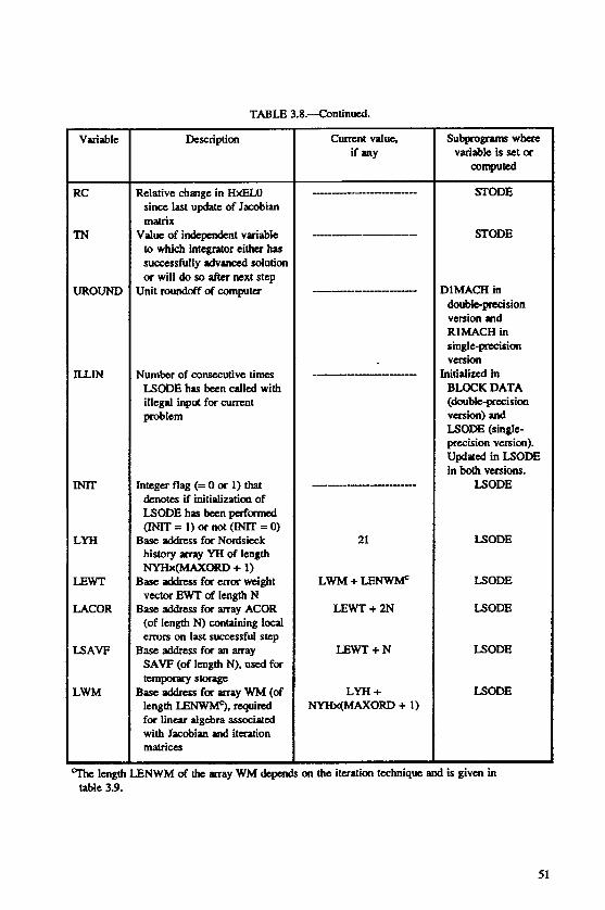
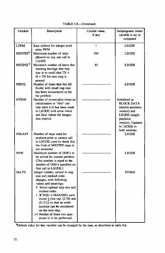
To further assist in user understanding and modification of the code, we have included in table 3.6 the names of all subprograms that use each common block. For the same reason we provide in tables 3.7 and 3.8 complete descriptions of the variables in EHOOO1 and LSOOO1, respectively. Also given for each variable are the default or current value, if any, and the subprogram (or subprograms) where it is set or computed. The length L E N W of the array WM in table 3.8 depends on the iteration technique and is given in table 3.9 for each legal value of MITER.
3.4 Special Features
The remainder of this chapter deals with the special features of the code and its built-in options. We also describe the procedure used to advance the solution by one step, the corrective actions taken in case of any difficulty, and step size and method order selection. In addition, we provide detailed flowcharts to explain the computational procedures. We conclude this chapter with a brief discussion of the error messages included in the code.
46
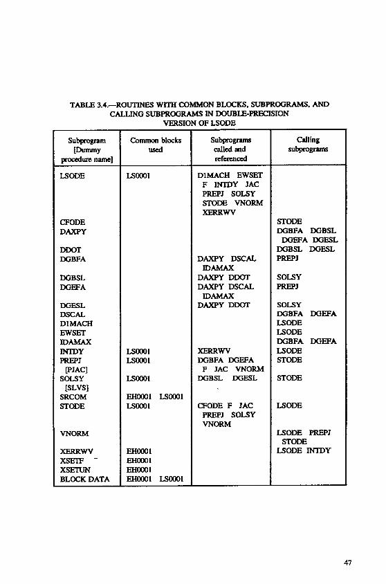
TABLE 3A.-ROUTINES 'WITH COMMON BLOCKS. SUBPROGRAMS, AND CALLING SUBPROGRAMS IN DOUBLECPRECISION
VERSION OF LSODE
LSODE
CFODE DAXPY
DDOT DGBFA
DGBSL DGEFA
DGESL DSCAL DIMACH EWSET I D m INTDY PREPJ
IPJACI SOLSY
[SLVS] SRCOM STODE
WORM
XERRW xsm -
x s m BLOCK DATA
Common blocks used
LSOoOl
EHOOOl EHo00l EHOOOl EHOOOl LSOOOl
DlMACH EWSET F INTDY JAC PREPJ SOLSY STODE WORM XERRW
DAXPY DSCAL
DAXPY DDOT DAXPY DSCAL.
DAXPY DDOT
IDAMAX
IDAMAX
mRRw DGBFA DGEFA
DGBSL DGESL F JAC WORM
CFODE F JAC PREPJ SOLSY WORM
Calling ~Ubprograms
STODE DGBFA DGBSL
DGEFA DGESL DGBSL DGESL PREF'J
SOLSY PREPJ
SOLSY DGBFA DGEFA LSODE LSODE DGBFA DGEFA LSODE STODE
STODE
LSODE
LSODE PREPJ
LSODE INTDY STODE
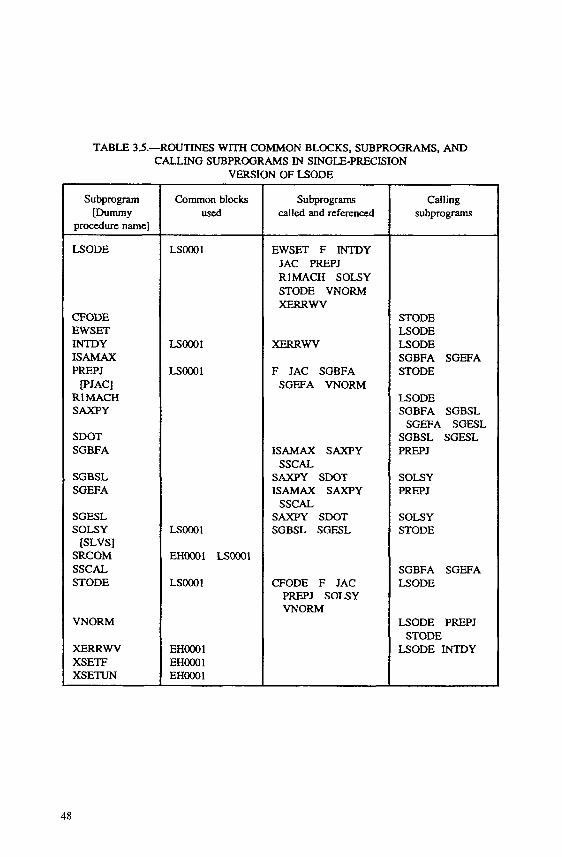
TABLE 3.5.-ROUTINES WITH COMMON BLOCKS. SUBPROGRAMS, AND CALLING SUBPROGRAMS IN SINGLE-PRECISION
VERSION OF LSODE
Subprogram [Dummy
procedure name]
LSODE
CFODE EWSET INTDY ISAMAX PREPJ
[PJACI R1 MACH SAXPY
SDOT SGBFA
SGBSL SGEFA
SGESL SOLSY
[SLVS] SRCOM SSCAL STODE
VNORM
XERRWV XSETF XSETUN
Common blocks used
LSOOOl
LSOOOI
LSOOOl
LSOOOl
EHOOOl LSOOOl
LSOOOl
EHOOO 1 EHOOO 1 EHOOOI
Subprograms called and referenced
EWSET F INTDY JAC PREPJ RIMACH SOLSY STODE VNORM XERRWV
xF,RRwv
F JAC SGBFA SGEFA VNORM
ISAMAX SAXPY
SAXPY SDOT ISAMAX SAXPY
SAXPY SDOT SGBSL SGESL
SSCAL
SSCAL
CFODE F JAC PREPJ SOLSY VNORhi
Calling subprograms
STODE LSODE LSODE SGBFA SGEFA STODE
LSODE SGBFA SGBSL
SGBSL SGESL PREPJ
SGEFA SGESL
SOLSY PREPJ
SOLSY STODE
SGBFA SGEFA LSODE
LSODE PREPJ
LSODE INTDY STODE
common block
EHOOOl
LSOOOl
Vuiabks (dimsion) subprosrum whae used
MESFLG LUNIT
Variable
MESFLG
LUNlT
CONIT CRATE EL(13) ELCO(13. 12) HOLD RMAX TESC0(3,12) CCMAX EL0 " M I N HMXIHURC TN UROUND ILLIN INIT LYH LEWT LACm LSAVFLWM LIWM MXSTEP -NIL "NIL NTREP N S M T " IALTHIKlpLMAx ME0 NQNYH NSLP ICF IERF'J IERSL JCUR JSTART KFLAGL METH MITER MAXORD MAXCOR MSBP MXNCF N NQ NST NFJ3 NJE NOU
Dcdaiption
Integer flag, which controls printing of tcrot messages from code and has following values and meanings: 0 No amr message is printed. 1 All emr messages ae printed.
Logical unit number for mcssagts from code
SRCOM XERRWV XSETF x s m BLOCK DATA'
LSODE INTDY PREPJ SOFSY SRCOM STODE B m K DATA'
%ouble-ptecision version only.
TABLE 3.7.-DESCRlPTION OF VARIABLES IN COMMON BLOCK EHOOO1. THEIR CURRJ34T VALUES. AND SUBPROGRMIS WHERE THEY ARE SET -
cumnt V d U e
1
6
subprognm- variabie is sct
BLOCK DATA in double-precision version
precision version and XERRW in single-
BLOCK DATA in double-precision vasion and XERRW in single- precision version
49
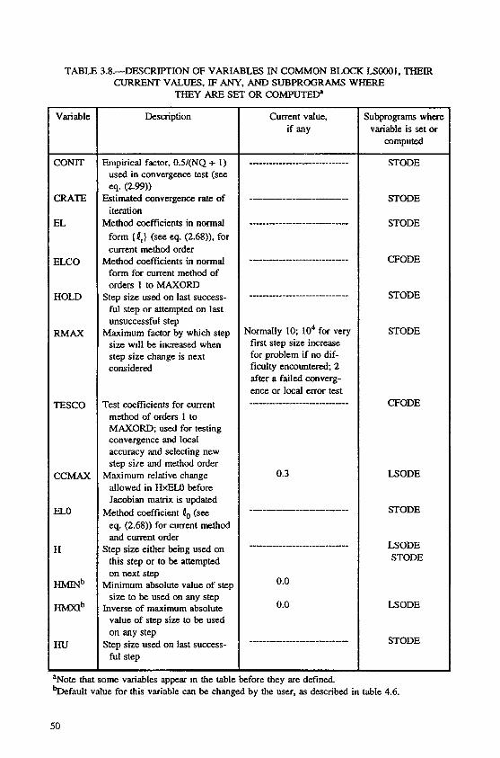
TABLE 3.8.-DESCRPTION OF VARIABLES LN COMMON BLOCK LSOOO1. THEIR CURRENT VALUES. IF ANY, AND SUBPROGRAMS WHERE
THEY ARE SET OR COMPUTED.
Variable
3ONlT
:RATE
?L
ZLCO
HOLD
M A X
mco
3CMAX
EL0
H
"b
HMMb
H u
Description
Empirical factor. 0.5/(NQ + I ) used in convergence test (see
Estimated convergence rate of
Method coefficients in normal
eq. (2.99))
iteration
form [ QI} (see eq. (2.68)), for current method order
Method coefficients in normal form for current method of orders 1 to MAXORD
Step s i x used on last success- ful step or attempted on last unsuccessful step
Maximum factor by which step size will be increased when step size change is next considered
Test coefficients for current method of orders 1 to MAXORD, used for testing convergence and local accuracy and selecting new step size and method order
allowed in HxELO before Jacobian matrix is updated
eq. (2.68)) for current method and current order
Step size either being used on this step or to be attempted on next step
Minimum absolute value of step size to be used on any step
Inverse of maximum absolute value of step size to be used on any step
Step size used on last success- ful step
Maximum relative change
Method coefficient Po (sw
Current value, if any
vmaliY IO; 104 for very first step size increasc for problem if no dif- ficulty encountered. 2 after a failed converg- ence or local error test
0.3
0.0
0.0
Subprograms where variable is set or
computed
STODE
STODE
STODE
CFODE
STODE
STODE
CFODE
B O D E
STODE
LSODE STODE
B O D E
STODE
"Note that some variables appear in the table before they are defined. h f a u l t value for this variable can be changed by the user, as described in table 4.6.
50
Variable
RC
TN
UROUND
ILLIN
m
LYH
LEWT
LACOR
LSAVF
LWM
TABLE 3.8.--Continued.
Description
Relative change in HxELO since last updatc of Jacobian matrix
Value of indcpcndcnt variable to which integrator cithw has successfully advanced solution or will do so aftcr next step
Unit roundoff of computer
Number of consecutive times LSODE has bccn called with illegal input for cumnt pcoblcm
Integer flag (= 0 or 1) that dmotes if initialization of LSODE has bccn paformcd ( IN lT=1)ornOt ( IN IT=O)
"X(MAx0RD + 1)
vector EWT of length N
(of length N) containing local e m on last succcssN step
Base lddrca fa Nordsicck history m y YH of length
Base ddrcss for e m weight
Base address for array ACOR
Base address for an array S A W (of length N). used for tempwary skn'agc
Base lddress f a array WM (of length LENWMC). required for linear algebra associated with Jacobian md itaztion d C e S
c u m t value, if any
21
LWM + L E W
LEWT + 2N
LEWT+N
LYH + "x(MAx0RD + 1)
%e. length table 3.9.
of the array WM depends on the iteration technique i
subprograns whue variable is set or
ComPuM
STODE
STODE
DlMACH in doubk-precision version md RlMACH in single-peckion version
BLOCK DATA (doubk-precision version) md LSODE (single- precision version). Updated in LSODE in both versions.
LSODE
Initialized in
LSODE
LSODE
LSODE
LSODE
LSODE
~~
I is given in
51
Variable
LIWM
MXSTEPb
MXHNILb
" N I L
NTREP
NSLAST
NYH
IALTH
TABLE 3.8.4ontinued.
Description
Base address for integer work
Maximum number of steps - Y M
allowed on any one call to LSODE
warning message that step s i x is so small that TN + H = TN for next step is p n n d
Maximum number of timcs that
Number of times that this dif- ficulty with small step size has been encountered so far for problem
Number of consecutive times an initialization or "first" call (see table 4.3) has been made to LSODE with same initial and final values for integra- tion interval
Number of steps used for problem prior to current call to LSODE; used to check that the limit of MXSTEP steps is not exceeded
Maximum number of ODE's to be solved for cumnt problem (This number is qua l to the number of ODE's specified on first call to LSODE.)
size and method order changes, with following valus and meanings: 0 Sclcct optimal step size and
method order. 1 If NQU < W O R D , save
v e d ~ 4 (sec cqs. (2.76) and (2.1 11)) so that an orda incnasc can be considered on the next step.
>I Neither of these two oper- ations is to be performed.
Integer counter, related to step
Cumnt value, if my
1
500
10
befault value for this variable can be changed by the user, as described in
52
subprograms when variable is set or
computed
LSODE
LSODE
LSODE
LSODE
[nitialized in BLOCK DATA (double-precision version) and LSODE (single- precision version). Updated in LSODE in both versions.
LSODE
LSODE
STODE
ble 4.6.
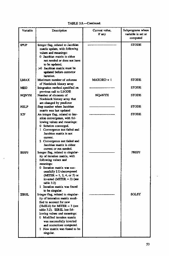
TABLE 3.8.4ntinued.
Variable Description
Integer flag, related to Jacobian matrix update, with following values and meanings: 0 Jacobian matrix is cithcs
not needed a does not have c O b e U p d . t e s
updated before comdor >o J 4 ; n matrix must be
ilcration. Maximum number of columns
of Nordsicck history m y Integration method specif& on prtvious u l l to LSODE
Number of elemnts of Nonfsicck history array that arc changed by predictor
Step numba when Jacobian matrix was last updated
An intega flag. related to iter- ation amvergenct. with fol- lowing values and meanings: 0 Solution converged. 1 Convergence test failed ud
Jacobian rmhix is not arrrmt.
2 Convergence test failed and Jacobian matrix is either current or not needed.
Integer flag. related to singulr- ity of iteration matrix, with following values and meanings: 0 llefation m - x w s suc-
assfully LUdecompoMd @mER = 1. 2.4, or 5 ) or invacad (MITER = 3) (set table 3.2)
1 llentionmntrixwsfound to be singular.
Integer flag, related to singular- ity of interation nubix modi- fied to BCUnmt for new (HxELo)forMrrER=3(set table 3.2). IERSL has fol- lowing vdues and munings: 0 M o d i d iteration matrix was successfully inverted and corrections computed.
1 New matrix was found to be singular.
Cumnt value, if any
W O R D + 1
NQxNYH
STODE
STODE
STODE
STODE
STODE
STODE
PREPJ
SOLSY
53
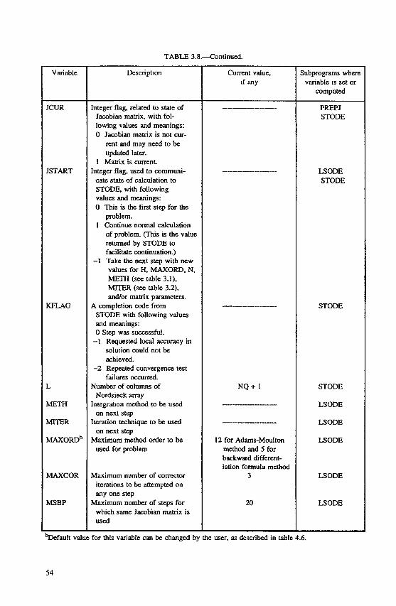
TABLE 3.8.--Continued.
Variable
[CUR
ISTART
(FLAG
W?TH
MITER
W O R D b
UAXCOR
MSBP
Description
Integer flag, related to state of Jacobian matrix, with fol- lowing values and meanings: 0 Jacobian matrix is not cur-
rent and may need to be updated later.
1 Matrix is cumnt. Integer flag, used to communi-
cate state of calculation to STODE. with following values and meanings: 0 This is the first step for the
I Continue n m a l calculation problem.
of problem. (This is the value returned by STODE to facilitate continuation.)
-1 Take the next step with MW values for H, MAXORD. N, hiETH (see table 3.1). MITER (see table 3.2). and/or matrix parameters.
A completion code from STODE with following values and meanings: 0 step was sucassful.
-1 Rtquestcd local accuracy in solution could not be achieved.
-2 Repeated convergence test failures occurred.
Number of columns of
Integration method to be used
Iteration technique to be used
Maximum method order to be
Nordsicxk array
on next step
on next step
used for problem
Maximum number of corrector iterations to be attempted on any one step
Maximum number of steps for which same Jacobian matrix is used
Current value, if any
-I-__
NQ+ I
12 for Adams-Moulton method and 5 for backward differcnt- iation formula method
3
a
hbprograms where variable IS set or
computed
PREPJ STODE
LSODE STODE
STODE
STODE
LSODE
LSODE
LSODE
LSODE
B O D E
Default value for this variable can be changed by the user. as described in table 4.6.
54
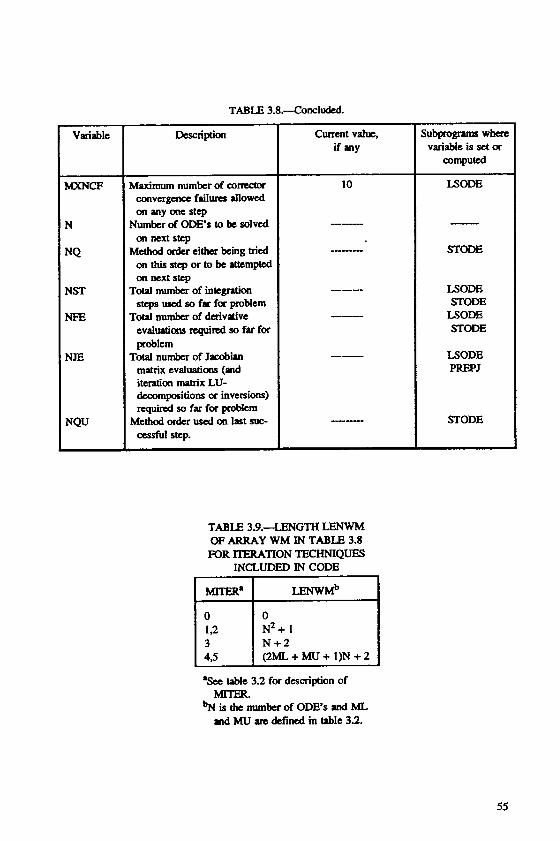
Variable
MXNCF
N
NQ
NST
NFE
N E
NQU
Dcmiption Cumnt value, if any
Maximum number of corndoc convergcllce fiiluret allowed on any OM step
Number of ODE'S to be SOlvtd on next step
Method order eithcr being tried on this step or to be attempted on next step
steps used so far for problem Total number of inlegdon
Total number of daivrive evaluations requid so far for problem
Total number of Jocobirn matrix evaluations (and iteration matrix LU- decompositions or inversions)
Method ordcr uscd on last suc- required so far for probIern
cessful step.
TABLE 3.9.-LENGTH LENWM OF ARRAY WM IN TABLE 3.8 FOR lTERATION "NIQW
INCLUDED IN CODE
MITER. I LENwMb I
4.5 (2ML+MU+I)N+2
iubprogrpns whac variable is set or
COmpUtCd
LSODE
- STODE
LSODE STODE
LSODE STODE
LSODE PREPJ
STODE
'See table 3.2 for description of MITER.
% is the number of ODE'S and ML md MU a defined in table 33.
55
3. Description of Code
The main routine, LSODE, controls the integration and serves as an interface between the calling subprogram and the rest of the package. A flowchart of this subroutine is given in figure 3.2. In this figure ITASK and ISTATE are user- specified integers that specify, respectively, the task to be performed and the state of the calculation, that is, if the call to LSODE is the first one for the problem or a continuation; if the latter, ISTATE further indicates if the continuation is a normal one or if the user has changed one or more parameters since the last call to LSODE (see chapter 4 for details). On return from LSODE the value of ISTATE indicates if the integration was performed successfully, and if not, the reason for failure. The integer JSTART is an internally defined variable used for communicating the state of the calculation with the routine STODE. The variables T (= C), H, and X are, respectively, the independent variable, the step size to be attempted on the next step, and the numerical solution vector. TOUT is the 6 value at which the solution is next required. Finally, TCRIT is the 5 value that the integrator must not overshoot. This option is useful if a singularity exists at or beyond TCRIT and is discussed further in chapter 4.
The subroutine STODE advances the numerical solution to the ODE’S by a single integration step [5,-1,E,,]. It also computes the method order and step size to be attempted on the next step. The efficiency of the integration procedure is increased by saving the solution history, which is required by the multistep methods used in the code, in the form suggested by Nordsieck (ref. 33). The Nx(q + 1) Nordsieck history matrix z,-l at cn-l contains the numerical solution L - 1 and the q scaled derivatives hiX$?~/j! 0’ = 1, ...,q), where h, (= 5, - E,,-1) and q are, respectively, the current step size and method order and 9) = djxJd5J.
The flowchart of STODE is presented in figure 3.3. In this figure NCF is the number of corrector convergence failures on the current step, KFLAG is an internally defined integer used for communication with LSODE, NQ (= q) is the method order to be attempted on the current step, and the integer counter IALTH indicates how many more steps are to be taken with the current step size and method order. The (NQ + 1)-dimensional vector contains the method coefficients and depends on both the integration method and the method order; 40 is the zeroth component of 1 (see eq. (2.68)). The matrix ziol is the predicted Nordsieck history matrix at E,,, and the NxN iteration matrix P is given by equation (2.25). The variable R is the ratio of the step size to be attempted next to its current value, M A X is the maximum R allowed when a step size change is next considered, and HMIN and HMAX are user-supplied minimum and maximum absolute values for the step size to be tried on any step. The ratios RHDN, RHSM, and RHUP are factors by which the step size can be increased if the new method order is NQ - 1, NQ (the current value), and NQ + 1, respectively. Finally, NQMAX is the maximum method order that may be attempted on any step, and the vector E, (=h,%, - h y lo1 ) is proportional to the local truncation error vector at 5, (see eqs. (2.87) an375.89)).
56
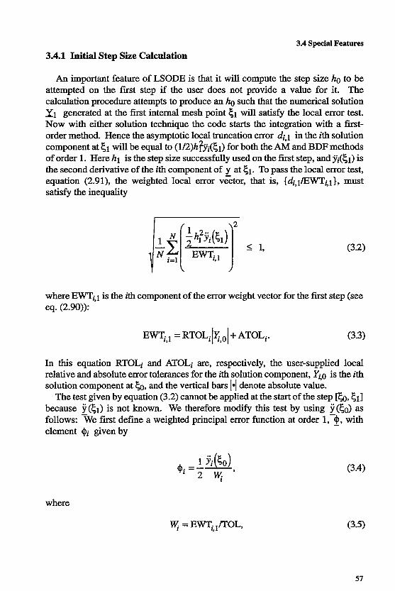
3.4 Special Features
3.4.1 Initial Step Size Calculation
An important feature of LSODE is that it will compute the step size ho to be attempted on the first step if the user does not provide a value for it. The calculation procedure attempts to produce an ho such that the numerical solution X1 generated at the first internal mesh p i n t 51 will satisfy the local error test. Now with either solution technique the code starts the integration with a first- order method. Hence the asymptotic local truncation error d j , ~ in the ith solution component at 51 will be equal to (1/2)h12jii(51) for both the Ah4 and BDF methods of order 1. Here hl is the step size successfully used on the first step, andy'i(s1) is the second derivative of the ith component of y at 51. To pass the local error test, equation (2.91), the weighted local error vector, that is, {~,,J/EWTL~}, must satisfy the inequality
where EWTil is the ith component of the error weight vector for the first step (see eq. (2.90)):
EWT,,~ = R T O L , I ~ , ~ I + ATOL,. (3.3)
In this equation RTOLi and ATOLi are, respectively, the user-supplied local relative and absolute error tolerances for the ith solution component, YLO is the ith solution component at 50, and the vertical bars 1.1 denote absolute value.
The test given by equation (3.2) cannot be applied at the start of the step [b, 511 because y(E,l) is not known. We therefore modify this test by using y(50) as follows: -We first define a weighted principal error function at order l,-$, - with element $i given by
$. =--I-, 1 Y.(50) ' 2 y. (3.4)
where
y. = Em,, /TOL, (3.5)
57
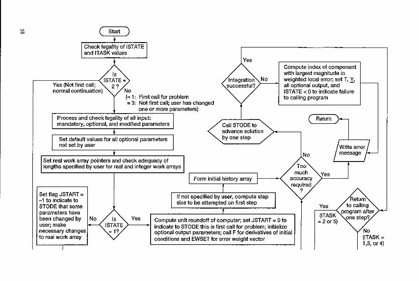
Start
Check legality of ISTATE and ITASK values
t
Compute index of component with largest magnitude in weighted local error; set T, all optional output, and ISTATE c 0 to indicate failure to calling program
- Yes (Not first call; normal continuation)
(= 1 : First call for problem = 3: Not first call; user has changed
one or more parameters)
Process and check legality of all input: mandatory, optional, and modified parameters
Set default values for all optional parameters not set by user
t Set real work array pointers and check adequacy of lengths specified by user for real and integer work arrays
Return Call STODE to
t advance solution
Form initial history array - t A Set flag JSTART = -1 to indicate to STODE that some parameters have been changed by user; make necessary changes to real work array
I Y If not specified by user, compute step size to be attempted on first step
Compute unit roundoff of computer; set JSTART = 0 to indicate to STODE this is first call for problem; initialize optional output parameters; call F for derivatives of initial conditions and EWSET for error weight vector
to calling
(ITASK = 1,3, or 4)
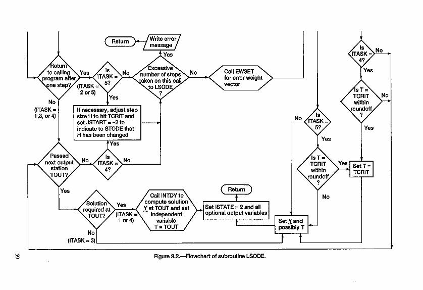
Call EWSET for error weight vector
Yes
If necessary, adjust step size H to hit TCRlT and
indicate to STODE that H has been changed
Set JSTART = -2 to
+ Yes
within
I Yes
1 Yes I IS T =
within
No Y \ T-TOUT / (ITASK = 3) I t
VI \o Figure 3B.-Flowchart of subroutine LSODE.
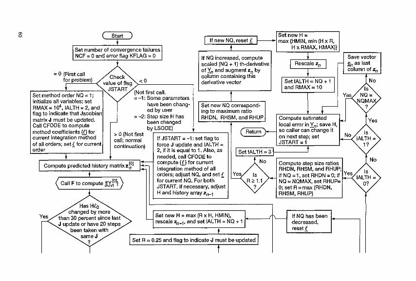
= 0 (First call
I for problem)
I Set new H = I max {HMIN, min (H x R, 4
If NQ increased, compute scaled (NQ + 1) th-derivative of and augment r,! by column containing this derivative vector
RMAX = 1 d, IALTH = 2, and flag to indicate that Jacobian matrix J must be updated. Call CFODE to compute method coefficients @for current integration method of all orders; set C for current
t = -1 : Some parameters have been chang- initialize all variables; set I I Set new NQ corresaond- I
I I I RHDN, RHSM, and RHUP I ing to maximum ratio ed by user = -2: Step size H has
1 beenchanged I I
b! > 0 (Not first call; normal continuation)
A Has He,-,
SODE)~ c If JSTART = -1 : set flag to force J update and IALTH = 2, if it is equal to 1. Also, as needed, call CFODE to compute {i} for current integration method of all orders; adjust NQ, and set 1 for current NQ. For both JSTART, if necessary, adjust H and history array z,-1
( Return?
Set IALTH = NQ + 1 and RMAX= 10
Compute estimated local error in L; save H, so caller can change it on next step; set JSTART = 1
I Set IALTH = 3 1 Compute step size ratios I RHDN. RHSM. and RHUPI
IS )-I if NQ = 1, set RHDN = 0; if’ R 2 1.1 NQ = NQMAX. set RHUP= v 0; set R = m a i (RHDN, I RHSM. RHUP)
changed bymore Set new H = max (R x H, HMIN), rescale q-1 , and set IALTH = NQ + 1 f& J update 30 percent or have s i n c e 3 20 steps
been taken with same J
+ Set R = 0.25 and flag to indicate J must be updated
t
J decreased,
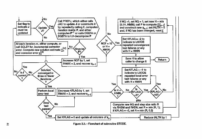
iteration matrix P, and either computes or calls DGEFA or DGBFA to LU-decompose P
At each iteration m, either compute, or call SOLSY for, incremental corrector [ml test failures or any error. Compute new solution estimate & and corrector errordd
with H = HMlN
Save H to allow caller to change it
RMAX = 2, and recover t Set KFLAG = -1 to indicate to LSODE - repeated local error - test failures or any with H = HMlN
RMAX = 2, and recover zn-l
via RHSM and RHDN; set R = min (R, 1);
Figure 3.3.4lowchart of subroutine STODE.
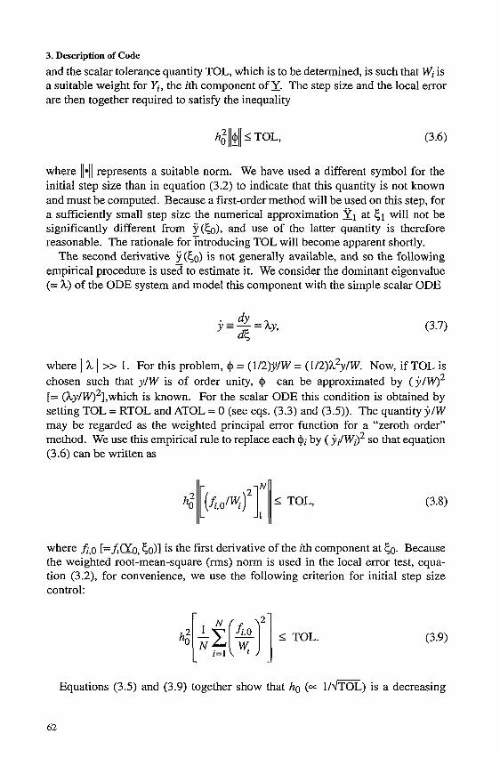
3. Description of Code
and the scalar tolerance quantity TOL, which is to be determined, is such that Wi is a suitable weight for Yi, the ith component of 1. The step size and the local error are then together required to satisfy the inequality
where 11-11 represents a suitable norm. We have used a different symbol for the initial step size than in equation (3.2) to indicate that this quantity is not known and must be computed. Because a first-order method will be used on this step, for a sufficiently small step size the numerical approximation 21 at 51 will not be significantly different from y(b), and use of the latter quantity is therefore reasonable. The rationale for h o d u c i n g TOL will become apparent shortly.
The second derivative y(50) is not generally available, and so the following empirical procedure is use3 to estimate it. We consider the dominant eigenvalue (= A) of the ODE system and model this component with the simple scalar ODE
where I h I >> 1. For this problem, I$ = (1/2)y/W = (1/2)h2y/W. Now, if TOL is chosen such that y/W is of order unity, I$ can be approximated by (y/W2 [= (Ay/W)2],which is known. For the scalar ODE this condition is obtained by setting TOL = RTOL and ATOL = 0 (see eqs. (3.3) and (3.5)). The quantity y/W may be regarded as the weighted principal error function for a “zeroth order” method. We use this empirical rule to replace each @ j by ( yJWj)2 so that equation (3.6) can be written as
N
h i [(&,O/yr] 1 I TOL,
where 3,o [=A(&, Eo)] is the first derivative of the ith component at 50. Because the weighted root-mean-square (rms) norm is used in the local error test, equa- tion (3.2), for convenience, we use the following criterion for initial step size control:
Equations (3.5) and (3.9) together show that ho (= 1 / m L ) is a decreasing
62
3.4 Special Features function of TOL. To produce a reliable estimate for h~ we therefore select a TOL erring on the high side. A suitable value is given by
TOL = max(RTOLi). (3.10) i
This expression cannot be used if all RTOLi = 0. In this case an appropriate value for TOL is given by
/ \
ATOL, TOL = maxi - for q,o f 0. (3.1 1)
In any case the value of TOL is constrained to be within reasonable bounds as follows:
loou I TOL I (3.12)
where u is the unit roundoff of the computer or the machine epsilon (ref. 13). It is the smallest positive number such that 1 + u > 1.
Equation (3.9) cannot be used to compute ho if either each fi,o is equal to zero or the norm is very small. To produce a reasonable ho in such an event, we include the independent variable 5 as the zeroth component yo of - y and modify equation (3.9) as follows:
(3.13)
where we have used the fact that y o = 1. To be consistent with the other Wi, which are of order Yio, the weight Wo should be of order 50; however, we use
(3.14)
to ensure that it is not equal to zero. In equation (3.14), &,utl is either the first (or only) value of the independent variable at which the solution is required or, as discussed in chapter 4, a value that gives both the direction of integration (i-e., increasing or decreasing 5) and an approximate scale of the problem. If the quantity &,ut, 1 - 50 is not significantly different fiom zero, an error exit occurs. Equation (3.13) gives a reasonable value for ho (= Wo m L ) if fo = 0.
63
3. Description of Code
The calculation procedure used for ho is therefore given by
TOL N 2
i=l N
(3.15)
Several restrictions apply to the step size given by equation (3.15). It is not allowed to be greater than the difference Icout,l - 501. Hence
In addition, if the user has supplied a value for h,,, the maximum step size to be used on any step, ho is restricted to
ho t- min(ho,h,,). (3.17)
However, no comparison of ho is made with hmin. the user-supplied minimum step size to be used on any step, so that ho is allowed to be less than hmin. Finally the sign of ho is adjusted to reflect the direction of integration.
3.4.2 Switching Methods
Another useful feature of LSODE is that different integration methods and/or different iteration techniques can be used in different subintervals of the problem. This option is useful when the problem changes character and is stiff in some regimes and nonstiff in others as, for example, in combustion chemistry. Indeed, because stiff problems are usually characterized by a nonstiff initial “transient” region, the ability to switch integration methods is a desirable feature of any ODE package. During the course of solving a problem the method flag MF may be changed both whenever and as many times as desired. As described in chapter 4 changing methods is quite straightforward.
3.4.3 Excessive Accuracy Specification Test
At each integration step Cn] LSODE checks that the user has not requested too much accuracy for the precision of the machine. This condition is said to occur if the criterion
? di,n < uq,n (3.18)
is true for all N solution components. In equation (3.18), di,n is the estimated
64
3.4 Special Features
local truncation error in Yi,m the ith solution component at cn. Now the numerical solution X at Z& is judged to be sufficiently accurate if the following inequality is satisfied (see chapter 2):
(2.9 1)
The quantity EWTb is the ith component of the error weight vector, equa- tion (2.90), for this step. Equations (3.18) and (2.91) together imply that if the quantity TOLSF (tolerance scale factor) defined as
(3.19)
is greater than 1, the test for excessive accuracy requirement is passed. This test is quite inexpensive, but it can be applied only after the solution at c n is produced. It is, however, wasteful to generate a solution only to discover that excessive accuracy has been required, either because TOLSF is greater than 1 or because repeated convergence failures or error test failures occur. The computational cost can be significant if any difliculty is encountered because of the corrective actions-described later in this section-performed by the code. Even if the step is successful, the solution is not meaningful because of roundoff errors.
To avoid these difficulties, the calculation procedure for TOLSF uses L-1, which is known, so that the test can be applied at the start of each step, including the first. Thus the code ascertains inexpensively if excessive accuracy has been requested before attempting to advance the solution by the next integration step. The value of TOLSF may be used to adjust the local error tolerances so that this condition does not recur. For example, scaling up the {RTOLi} and {ATOLi} values by a minimum factor of TOLSF should produce satisfactory values for the local error tolerances if the same type of error control is to be performed (see chapter 4 for details).
3.4.4 Calculation of Method Coefficients
The integration method coefficients and test constants used to check corrector convergence and local accuracy, as well as to select method order and step size, are computed in subroutine CFODE. The calculation procedure uses the generating polynomials discussed by Hindmarsh (refs. 21 and 22) to increase portability of the code. The coefficients corresponding to all method orders are computed and stored both at the start of the problem and whenever the user changes the integration method. This feature avoids the computational cost associated with recomputing these quantities whenever the method order is changed.
65
3. Description of Code
3.4.5 Numerical Jacobians
If Newton-Raphson (NR) or Jacobi-Newton (JN) iteration is selected, the code will generate elements of the Jacobian matrix by finite-difference approximations if the user chooses not to provide an analytical Jacobian. For the iteration procedures corresponding to MITER = 2 (full Jacobian matrix) and 5 ("banded" Jacobian matrix, Le., a matrix with many zero entries and all nonzero elements concentrated near the main diagonal), the element .Tu (= &/&?) at cn is estimated by using the approximation
fi ({do: + 6 k j A Y j } >tn) -fi ({e:} 9 k n )
J.. z= , i = l , ..., N , (3.20) B - AYj
where Y[$:n is the kth component of YLol, Fkj is the Kronecker symbol,
kJ = { O > 1, k = k # j j , (3.2 1)
and the increment A q in the jth solution component is selected as follows: The standard choice for AYj is
(3.22)
This equation cannot be used if is either equal to zero or very small. Therefore an alternative value, based on noise level, is deduced as follows: Now the error in eachfi due to roundoff is of order ulfil. Hence in replacing afi//ayi by the difference quotient, equation (3.20), the resulting element Ji/ has an error of order uKl/rj, where for clarity in presentation we have replaced Ayi by 5. Finally because the method coefficient 00 (= 40) is of order unity (see tables 2.1 and 2.2), the error FPo in the element Po of the iteration matrix P, equation (2.25), is approximately
If we introduce the N-dimensional column vector s, with element sj defined as
s - = l / r . , j =1 , ..., N, (3.24) J J
the matrix FP containing the errors { FPu} is given by
66
3.4 Special Features
6P = IhI u I f l sT , (325)
where I f I is an N-dimensional column vector containing the absolute values of the (i = 1, ...m and the superscript Tindicates transpose. A suitable increment 9 is
obtained by bounding la, as discussed next. To be consistent with the corrector convergence test, equation (2.98), and the
local error test, equation (2.91), we use the weighted rms norm, which for an arbitrary N-dimensional column vector ~1 is given by
If re introduce th
2 N
diagonal matrix D of order N, with element Dii given by
Dii = l/EWi, i = 1, ..., N, (327)
it is easily verified that
= llDZll,/J;;. (3.28)
where 11.11, is the Euclidean norm, defined for as
Now the norm of 6P is given by
where
because 6P is of rank 1. Hence
(3.30)
(3.3 1)
67
3. Description of Code
which can be rewritten as
(3.32)
To establish the maximum allowable error in P, we consider the linear system PL = b, which is the form of the equation to be solved at each Newton iteration, equation (2.24). To first order, the error 6~ in x due to the error 6P in P is given by (e.g., ref. 13)
(3.33)
The norm P-' I is not known but is expected to be of order unity because P + I, the identity matrix of order N , when h + 0 and P - -hPoJ when h -+ 00 (see eq. (2.25)). Therefore, a reasonable strategy is to bound I 6P I alone by selecting a suitably small value for the relative error that can be tolerated in the Newton correction vector. By using a value of 0.1 percent for this error, we obtain from equations (3.32) and (3.33)
(3.34)
For additional safety ro is reset to 1 if it is equal to zero. Finally the increment A 5 in thejth variable used to estimate the { J g } is given by
68
3.4 Special Features
(3.35) A$ = max JII q, Io EWT~,,). ( I I For a full Jacobian matrix the above procedure will require (N + 1) derivative
evaluations and can therefore become much more expensive than the use of an analytical Jacobian, especially for large N. Now fao1, is required by the corrector (see eq. (2.36)), irrespective of the iteration technique. Hence the use of MITER = 2 requires the evaluation of only N additional derivatives.
In generating the finitedifference banded Jacobian matrix (MITER = 5) the code exploits the bandedness of the matrix for efficiency. The number of additional derivative evaluations required to form the Jacobian matrix is only ML + MU + 1, where ML and MU are, respectively, the lower and upper half-bandwidths of the Jacobian matrix.
If JN iteration with MITER = 3 is used, the N diagonal elements Jii (i = 1, ...m are estimated by using the approximation
, i = 1 ,..., N, (3.36) J.. p I 1 A$
which requires only one additional derivative evaluation. The increment AYi is selected as follows: Now equation (2.17) shows that if functional iteration were used, the correction ~ 1 1 - 1$01 that would be obtained on the first iteration is equal to the quantity PO - g a o l ) , where the vector function - g is given by equa- tion (2.16). The increment vector AX is taken to be 10 percent of this correction:
A q = 0.1 pogi(xF1), i = 1, ..., N. (3.37)
Hence the diagonal matrix approximation, equation (3.36), resembles a directional derivative off taken in the same direction as the correction vector above. Also, this approximation gives the correct Jacobian if it is a
the magnitude of AYiis less than 0.lupo EWTi, that is, set equal to zero.
3.4.6 Solution of Linear System of Equations
If NR iteration is used for the problem, a linear system of the form PL = h must be solved for the correction vector 5 at each iteration (see eq. (2.24)). The linear algebra necessary to solve this equation is performed by the LU method (e.g.,
69
3. Description of Code
refs. 5 and 36), rather than by explicitly inverting the iteration matrix, which will require prohibitive amounts of computer time (ref. 13). In the LU method the iteration matrix is factored into the product of two triangular matrices L and U. Solving equation (2.24) then requires the fairly simple solution of two triangular linear systems in succession.
LSODE also includes special procedures for the LU-decomposition of the iteration matrix and the solution of equation (2.24) when the matrix is known to be banded. Compared to a full matrix, it is significantly less expensive to form a banded matrix, perform its LU-decomposition, and solve the linear system of equations (refs. 5,25,26, and 36). An important advantage of LU-decomposing a banded matrix over inverting it is that, besides being faster, the triangular factors L and U lie within nearly the same bands as the original matrix, whereas the inverse is a full matrix (ref. 36). This feature makes the computation of the correction vector significantly faster with the LU method than by premultiplying the right-hand side of equation (2.24) with the inverse of the matrix.
If MITER = 3 is used for the problem, the resulting iteration matrix is diagonal (see eq. (3.36)). Its inverse can therefore be obtained trivially and is used to compute the corrections.
3.4.7 Jacobian Matrix Update
The difficulty with Newton-Raphson iteration is the computational cost associated with forming the Jacobian matrix and the linear algebra required to solve for the correction vector at each iteration. However, as discussed in chap- ter 2, the iteration matrix need not be very accurate. This fact is exploited to reduce the computational work associated with linear algebra by not updating P at every iteration. For additional savings it is updated only when the iteration does not converge. Hence the iteration matrix is only accurate enough for the solution to converge, and the same matrix may be used over several steps. It is also updated if three or more error test failures occur on any step. Now P may be altered if the coefficient hPo is changed (see eq. (2.25)) because a new step size and/or method order is selected. In order to minimize convergence failures caused by an inaccurate P, the code updates P and performs its LU-decomposition (or inversion if MITER = 3) if hPo has changed by more than 30 percent since the last update of P. In addition, for MITER = 3, because P-' can be generated inexpensively, it is first modified to account for any change in hPo since its last update, before the corrections are computed. The reevaluation and LU- decomposition or inversion are also done whenever the user changes any input parameter required by the code. Finally the same P is used for a maximum number of 20 steps, after which it is reevaluated and LU-decomposed or inverted.
3.4.8 Corrector Iteration Convergence and Corrective Actions
Irrespective of the solution method and the corrector iteration technique, the maximum number of corrector iterations attempted on any step is set equal to 3,
70
3.4 Special Features
based on experience that a larger number increases the computational cost without a corresponding increase in the probability of successful convergence (refs. 19, 21,22, and 25). In addition to performing the convergence test, equation (2.99), at each iteration, STODE examines the value of the convergence rate c,, equa- tion (2.102). If c, is greater than l, the iteration is clearly not converging. STODE exploits this fact by abandoning the iteration if c, is greater than 2 after the second iteration.
If convergence is not obtained because either (1) equation (2.99) is not satisfied after three iterations or (2) c, > 2 after the second iteration, the following corrective actions are taken: For NR and JN iterations, if P is not current, it is updated at y =&.'I and LU-decomposed or inverted, and the step is retried with the same st.?, size. However, if either P is current or functional iteration is used, a counter of convergence failures on the current step is increased by 1, the step size is reduced by a factor of 4, and the solution is attempted with the new step size. The same corrective actions are taken in the event of a singular iteration matrix.
This procedure is repeated until either convergence is obtained or the integration is abandoned because either (1) 10 convergence failures have occurred or (2) the step size has been reduced below a user-supplied minimum value h-. In the event of an error exit the index of the component with largest magnitude in the weighted local error vector is returned to the subprogram calling LSODE.
3.4.9 Local Truncation Error Test and Corrective Actions
After successful convergence STODE performs the local truncation error test, equation (2.96). If the error test fails, the step size is reduced and/or the method order is reduced by 1 by using the procedures outlined in section 3.4.10, and the step is retried. After two consecutive failures the step size is reduced by at least a factor of 5, and the step is retried with either the same or a reduced order. After three or more failures it is assumed that the derivatives that have accumulated in the Nordsieck history matrix have errors of the wrong order. Therefore the first derivative is recomputed and the method order is set equal to 1 if it is greater than 1. Then the step size is reduced by a factor of 10, the iteration matrix is formed and either LU-decomposed or inverted, and the step is retried with a new z,-i that is constructed from L-1 and y,1= f&-1).
This procedure is repeated until either the error test is passed or an error exit is taken because either (1) 10 error test failures have occurred or (2) the step size has been reduced below h ~ , , . In the event of an error exit LSODE returns the index of the component with the largest magnitude in the weighted local error vector to the calling subprogram.
If the accuracy test is passed, the step is accepted as successful, and the Nordsieck history matrix z, and the estimated local truncation error vector & at & are computed by using equations (2.76) and (2.89), respectively. Irrespective of whether the step was successful or not, STODE saves the value of the most recent step size attempted on the step so that the user may, if desired, change it.
71
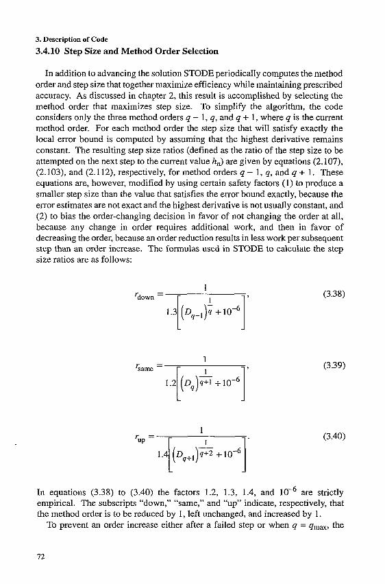
r----- -- ---- 3.4.10 Step Size and Method Order Selection
In addition to advancing the solution STODE periodically computes the method order and step size that together maximize efficiency while maintaining prescribed accuracy. As discussed in chapter 2, this result is accomplished by selecting the method order that maximizes step size. To simplify the algorithm, the code considers only the three method orders 4 - 1, 4, and 4 + 1, where 4 is the current method order. For each method order the step size that will satisfy exactly the local error bound is computed by assuming that the highest derivative remains constant. The resulting step size ratios (defined as the ratio of the step size to be attempted on the next step to the current value h,) are given by equations (2.107), (2.103), and (2.1 12), respectively, for method orders 4 - 1, q, and 4 + 1. These equations are, however, modified by using certain safety factors (1) to produce a smaller step size than the value that satisfies the error bound exactly, because the error estimates are not exact and the highest derivative is not usually constant, and (2) to bias the order-changing decision in favor of not changing the order at all, because any change in order requires additional work, and then in favor of decreasing the order, because an order reduction results in less work per subsequent step than an order increase. The formulas used in STODE to calculate the step
I (3.38) -
rdown - r 1 1’
I L J
L I 1
1’ r = I . up r 1
(3.39)
(3.40)
In equations (3.38) to (3.40) the factors 1.2, 1.3, 1.4, and are strictly empirical. The subscripts “down,” “same,” and “up” indicate, respectively, that the method order is to be reduced by 1, left unchanged, and increased by 1.
To prevent an order increase either after a failed step or when 4 = qmX, the
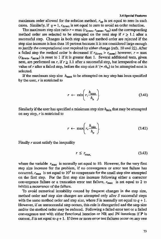
3.4 Special Features maximum order allowed for the solution method, rup is set equal to zero in such cases. Similarly, if q = 1, rdom is set equal to zero to avoid an order reduction.
The maximum step size ratio r = max (rdom, rsm, rup) and the corresponding method order are selected to be attempted on the next step if r 2 1.1 after a successful step. Changes in both step size and method order are rejected if the step size increase is less than 10 percent because it is not considered large enough to justify the computational cost required by either change (refs. 10 and 22). After a failed step the method order is decreased if ?-do, > rsm; however, r = max (rdom, r-) is reset to 1 if it is greater than 1. Several additional tests, given next, are performed on r, if r 2 1.1 after a successful step, but irrespective of the value of r after a failed step, before the step size h' (= rh,) to be attempted next is selected.
If the maximum step size hmax to be attempted on any step has been specified by the user, r is restricted to
r t min( r , ~ ) . (3.41)
Similarly if the user has specified a minimum step size h- that may be attempted on any step, r is restricted to
r t max ( r,- h c ) .
Finally r must satisfy the inequality
(3.42)
(3.43)
where the variable rmax is normally set equal to 10. However, for the very first step size increase for the problem, if no convergence or error test failure has occurred, rmax is set equal to lo4 to compensate for the small step size attempted on the first step. For the first step size increase following either a corrector convergence failure or a truncation error test failure, rmax is set equal to 2 to inhibit a recurrence of the failure.
To avoid numerical instability caused by frequent changes in the step size, method order and step size changes are attempted only after S successful steps with the same method order and step size, where S is normally set equal to 4 + 1. However, if an unsuccessful step occurs, this rule is disregarded and the step size andlor the method order may be reduced. Following a failed error test or a failed convergence test with either functional iteration or NR and JN iterations if P is current, S is set equal to 4 + 1. If three or more error test failures occur on any one
73
3. Description of Code
step, S is set equal to 5 even though the method order is reduced to 1. Finally following a step for which step size and method order changes are rejected because r < 1.1, S is set equal to 3.
After every S - 1 successful steps STODE saves the vector e, if q < qma, in order to estimate Ve, which is required to compute rup (see eqs. (2.109) to (2.112)). To minimize storage requirements, en is saved as the qmaxth, that is, the last, column of 2,.
3.5 Error Messages
The code contains many error messages-too numerous to list here. Every input parameter is tested for legality and consistency with the other input variables. If an illegal input parameter is discovered, a detailed message is printed. Each error message is self-explanatory and complete. It not only describes the mistake but in some instances tells the user how to fix the problem. Any difficulty encountered during execution will result in an error exit. A message giving the reason for termination will also be printed. If the computation stops prematurely, the user should look for the error message near the end of the output file corresponding to the logical unit number LUNIT (see chapter 4).
Chapter 4 Description of Code Usage
To use the LSODE package, the following subprograms must be provided: (1) a routine that manages the calls to subroutine LSODE, (2) a routine that computes the derivatives c f i = dyi/&} for given vdues of the independent variable 6 and the solution vector y , and (3) if an analytical Jacobian matrix J (= af/ay) is required by the corrector%eration technique selected by the user, a routine that computes the elements of this matrix. In addition, some modifications, discussed below, to the LSODE source itself may be necessary.
4.1 Code Installation
4.1.1 BLOCK DATA Variables
The user may wish to reset the values for the integer variables MESFLG (cur- rently l) and LUNIT (currently 6), which are both set either in the BLOCK DATA module (double-precision version) or in subroutine XERRWV (single-precision version). The variable MESFLG controls the printing of error messages from the code, and LUNIT is the logical unit number for such output (see table 3.7). Setting MESFLG = 0 will switch off all output from the code and therefore is not recommended.
The single-precision version of the code loads initial values for the common block LSOOOl variables ILLIN and NTREP (see table 3.8) through a DATA state- ment in subroutine LSODE. The same procedure is used in subroutine XERRWV for the common block EHOOOl variables MESFLG and LUNIT (see table 3.7). However, on some computer systems initial values for common block elements cannot be defined by means of DATA statements outside a BLOCK DATA subprogram. In this case the user must provide a separate BLOCK DATA subprogram, to which the two DATA statements from subroutines LSODE and XERRWV must be moved. The BLOCK DATA subprogram must also contain the two common blocks EHOOOl and LSOOOl (see table 3.6).
75
4. Description of Code Usage
4.1.2 Modifying Subroutine XERRWV
The subroutine XEFGXWV, which prints error messages from the code, is machine and language dependent. Therefore the data type declaration for the argument MSG, which is a Hollerith literal or integer array containing the message to be printed, may have to be changed. The number of Hollerith characters stored per word is assumed to be 4, and the value of NMES, which is the length of, that is, number of characters in, MSG is assumed to be a multiple of 4, and at most 60. However, the routine describes the necessary modifications for several machine environments. In particular, the user must change a DATA statement and the format of statement number 10. The routine assumes that all errors are either (1) recoverable, in which case control returns to the calling subprogram, or (2) fatal, in which case the run IS aborted by passing control to the statement STOP, which may be machine dependent. If a different run-abort command is needed, the line following statement number 100, which is located near the end of the routine, must be changed.
4.2 Call Sequence
The call sequence to subroutine LSODE is as follows:
CALL LSODE (F, NEQ, Y, T, TOUT, ITOL, RTOL, ATOL, ITASK, ISTATE, IOPT, RWORK, LRW, IWORK, LIW, JAC, MF)
All arguments in the call sequence are used on input, but only Y, T, ISTATE, RWORK, and IWORK are used on output. Also, Y and T are set only on the first call to LSODE; the other arguments may, however, have to be reset on subsequent calls. The arguments to LSODE are defined as follows:
F The name of the user-supplied subroutine that computes the derivatives of the dependent variables with respect to the independent variable. This name must be declared EXTERNAL in the subprogram calling LSODE. The requirements of subroutine F are described in section 4.3.
NEQ The number of first-order ordinary differential equations (ODE’s) to be solved. (The code allows the user to decrease the value of NEQ during the course of solving the problem. This option is useful if some variables can be discarded as the solution evolves as, for example, in chemical kinetics problems for which the reaction mechanism is reduced dynamically.) As discussed later, NEQ can be specified as an array. In this case NEQ(1) must give the number of ODE’s to be solved, and the subprogram calling LSODE must contain a dimension statement for NEQ.
76
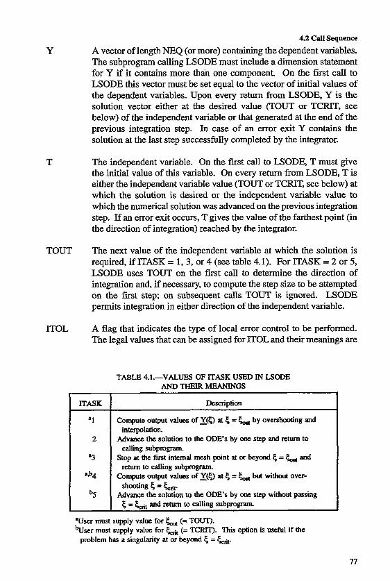
Y
T
TOUT
ITOL
4.2 Call Sequence
A vector of length NEQ (or more) containing the dependent variables. The subprogram calling LSODE must include a dimension statement for Y if it contains more than one component. On the first call to LSODE this vector must be set equal to the vector of initial values of the dependent variables. Upon every return from LSODE, Y is the solution vector either at the desired value (TOUT or TCRIT, see below) of the independent variable or that generated at the end of the previous integration step. In case of an error exit Y contains the solution at the last step successfully completed by the integrator.
The independent variable. On the first call to LSODE, T must give the initial value of this variable. On every rehun fi-om LSODE, T is either the independent variable value (TOUT or TCRIT, see below) at which the solution is desired or the independent variable value to which the numerical solution was advanced on the previous integration step. If an error exit occurs, T gives the value of the farthest point (in the direction of integration) reached by the integrator.
The next value of the independent variable at which the solution is required, if ITASK = 1, 3, or 4 (see table 4.1). For ITASK = 2 or 5, LSODE uses TOUT on the first call to determine the direction of integration and, if necessary, to compute the step size to be attempted on the first step; on subsequent calls TOUT is ignored. LSODE permits integration in either direction of the independent variable.
A flag that indicates the type of local error control to be performed. The legal values that can be assigned for ITOL and their meanings are
TABLE Il.-VALUES OF ITASK USED IN MODE ANDTHEIRMEANINGS
ITASK DeScriptiOn
+ I
2
'3
ab4
b5
Compute output valucs of I(<) ?t 5 = 5, by overshooting and
Advance the solution to the ODE'S by one step and =turn to
Stop at the first internal mesh point at or beyond 5 = f& and
c~mpule output values ofI(s> at 5 = 5, but without over-
Advance the solution to the ODE's by m step without passing
interpolation.
calling subprogram.
rcturn to calling subprogram.
shooting 5 = Lr 5 = $,, and return to calling subprogram.
.User must supply value for Lilt (= TOUT). bser must supply value for Lt (= TCRIT). 'Ihis option is useful if the
probIem has a singularity at or beyond 5 =
77
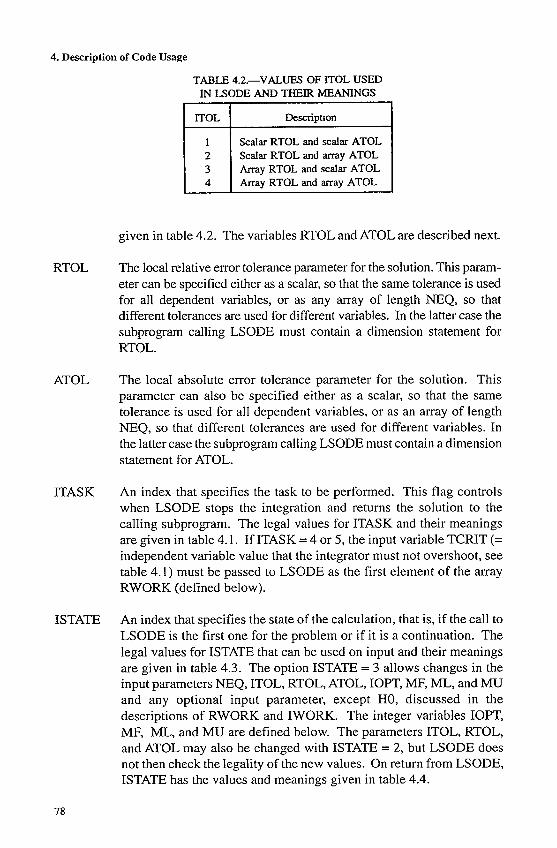
4. Description of Code Usage
TABLE 42-VALuES OF ITOL USED IN LSODE AND THEIR MEANINGS
Description
Scalar RTOL and scalar ATOL
Anay RTOL and scalar ATOL
given in table 4.2. The variables RTOL and ATOL are described next.
RTOL
ATOL
ITASK
ISTATE
78
The local relative error tolerance parameter for the solution. This param- eter can be specified either as a scalar, so that the same tolerance is used for all dependent variables, or as any array of length NEQ, so that different tolerances are used for different variables. In the latter case the subprogram calling LSODE must contain a dimension statement for RTOL.
The local absolute error tolerance parameter for the solution. This parameter can also be specified either as a scalar, so that the same tolerance is used for all dependent variables, or as an array of length NEQ, so that different tolerances are used for different variables. In the latter case the subprogram calling LSODE must contain a dimension statement for ATOL.
An index that specifies the task to be performed. This flag controls when LSODE stops the integration and returns the solution to the calling subprogram. The legal values for ITASK and their meanings are given in table 4.1. If ITASK = 4 or 5, the input variable TCRIT (= independent variable value that the integrator must not overshoot, see table 4.1) must be passed to LSODE as the first element of the array RWORK (defined below).
An index that specifies the state of the calculation, that is, if the call to LSODE is the first one for the problem or if it is a continuation. The legal values for ISTATE that can be used on input and their meanings are given in table 4.3. The option ISTATE = 3 allows changes in the input parameters NEQ, ITOL, RTOL, ATOL, IOPT, MF, ML, and MU and any optional input parameter, except HO, discussed in the descriptions of RWORK and IWORK. The integer variables IOF'T, MF, ML, and MU are defined below. The parameters ITOL, RTOL, and ATOL may also be changed with ISTATE = 2, but LSODE does not then check the legality of the new values. On return from LSODE, ISTATE has the values and meanings given in table 4.4.
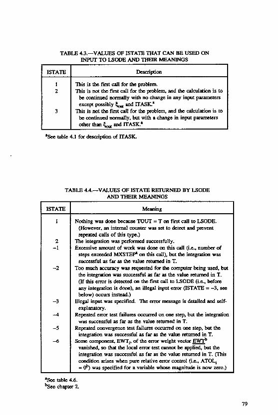
TABLE 4.3.-VALUES OF ISTATE THAT CAN BE USED ON INPUT TO LSODE AND THEIR MEANINGS
ISTATE Description I
1 2
3
This is the first call for the problem. This is not the first call for thc problem, and the calculation is to
be continued d l y with no change in any input parameters except possibly and ITASK?
This is not the first call for the problem, and the calculation is to be continued normally, but with a change in input parameters orher than E,,,,,, and f lAsIc.
'Set table 4.1 for description of ITASK.
TABLE 4.4.-VALUES OF ISTATE RETURNED BY LSODE
ISTATE
1
2 -1
-2
-3
-4
-5
-6
ANDTHEIRMEANINGS
Meaning
Nothing was done because TOUT = T on fust call to LSODE. (However, an internal counter was set to detect and prtvent repeated calls of this type.)
The integration was performed succcssfully. Excessive amount of work was done on this call (Le., number of
steps excttdcd MXSl" on this call), but the integration was successful as far as thc value returned in T.
Too much accucacy was requested for thc computer being used. but the integration was successful as far as the value returned in T. (If this error is detected on the first call to LSODE (Le., before any integration is done), an illegal input e m @!STATE = -3, see below) occufs instead.)
Illegal input was specified. The e m message is detailed and self-
Repeated error test failures occumd on one step, but the integration was successful as far as the value returned in T.
Repeated convergence test failures occumd on one step, but the integration was successful as far as the value retumcd in T.
Some component, mi.. of the error weight vector & vanished, so that the local e m test cannot be applied. but the integration was successful as far as thc value returned in T. (This condition arises when pure relative error control (is., ATOL, = ob) was specified for a variable whose magnitude is now zero.)
explanatory.
*Sa table 4.6. 4ke chapter 2.
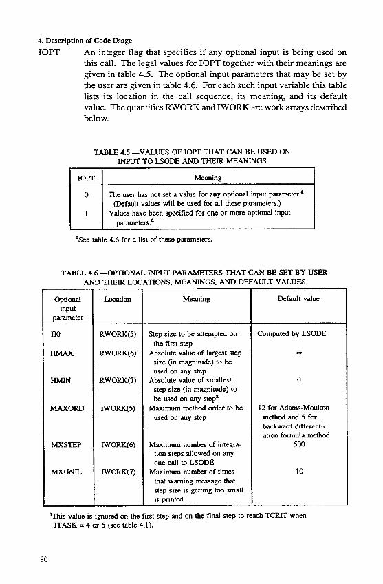
4. Description of Code Usage
IOFT An integer flag that specifies if any optional input is being used on this call. The legal values for IOPT together with their meanings are given in table 4.5. The optional input parameters that may be set by the user are given in table 4.6. For each such input variable this table lists its location in the call sequence, its meaning, and its default value. The quantities RWORK and WORK are work arrays described below.
TABLE 4.5.-VALUFS OF IOPT THAT CAN BE USED ON INPUT TO LSODE AND THEIR hEANWGS
The user has not set a value for any optional input parameter.' (Default values will be used for all thcsc parameters.)
Values have been specified for one or more optional input
table 4.6 for a list of these parameters.
TABLE 4.6.-OFTIONAL INPUT PARAMETERS THAT CAN BE SET BY USER AND THEIR LOCATIONS. MEANINGS. AND DEFAULT VALUES
op t id input
parameter
HO
HMAX
HMlN
MAXORD
MXSTEP
MXHNlL
Location
RWORK(5)
RWORK(6)
RWORK(7)
IWORK(5)
IWORK(6)
IWORK(7)
Meaning
Step size to be attempted on the first step
Absolute value of largest step size (in magnitude) to be used on any step
Absolute value of smallest step size (in magnitude) to
Maximum mcthod order to be be uscd on any step.
used on any step
Maximum number of integra- tion steps allowed on any one call to LSODE
Maximum numbcr of times that warning message that step size is getting too small is printed
Default value
Computed by LSODE
0
12 for Adams-Moulton method and 5 for backward differenti- ation formula method
500
10
value is ignored on the first step and on the final step to reach TCRlT when ITASK = 4 or 5 (see table 4.1).
80
RWORK
LRW
IWORK
LIW
JAC
4.2 Call !Sequence
A real work array used by the integrator. The subprogram calling LSODE must include a dimension statement for RWORK. If ITASK = 4 or 5, the user must set RWORK(1) = TCRIT (see table 4.1) to transmit this variable to LSODE. If any optional real input parameters are used, their values are also passed in this array to LSODE, the address for each of these parameters is given in table 4.6. Upon return from LSODE, RWORK contains several optional real output parameters. For each such output variable table 4.7 lists its location in RWORK and its meaning. In addition, the Nordsieck history array at the current value of the independent variable (TCUR in table 4.7) and the estimated local error vector in the solution incurred on the last successful step can be obtained from RWORK. Table 4.8 lists the names used for these two quantities and their locations in RWORK. In this table NYH is the value of NEQ on the first call to LSODE, and NQCUR and LENRW are both defined in table 4.7, which also gives their locations in the array WORK (see below).
Length of the real work array RWORK. Its minimum value depends on the method flag MF (see below) and is given in table 4.9 for each legal value of MF. In this table the integer W O R D is the maximum method order (default values = 12 and 5 for t h e m and BDF methods, respectively) to be used. The integers ML and MU are the lower and upper half-bandwidths, respectively, of the Jacobian matrix if it is declared to be banded (see table 3.2).
An integer work array used by the integrator. The subprogram calling LSODE must include a dimension statement for IWORK. If MITER (= second decimal digit of MF, defined below) = 4 or 5 (table 3.2), the user must set IWORK(1) = ML and IWORK(2) =MU (see descriptions above) to transmit these variables to LSODE. If any optional integer input parameters are used, their values are also passed in this array to LSODE; the address for each of these parameters is given in table 4.6. Upon return from LSODE, IWORK contains several optional integer output parameters. For each such output variable table 4.7 lists its location in WORK and its meaning.
Length of the integer work array IWORK. Its minimum value depends on MITER (table 3.2) and is given in table 4.10 for each legal value of MITER.
The name of the user-supplied subroutine that computes the elements of the Jacobian matrix. This name must be declared EXTERNAL in the subprogram calling LSODE. The form and description of sub- routine JAC are given in section 4.4.
81
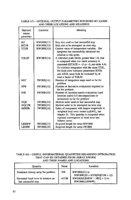
TABLE 4.7.-OPTIONAL OUTPUT PARAMETERS RETURNED BY LSODE AND THEIR LOCATIONS AND MEANINGS
Nordsieck history array for problem
Estimated local error in solution on last successful step
Optional output
parameter
Ku HCUR TCUR
TOLSF
NST
NFE
N E
NQU NQCUR IMXER
LENRW LENW
YH RWORK(21) to
ACOR RWORK(20 + NYH(NQCUR + 1))
RWORKCENRW) RWORK(LENRW - NEQ + 1) to
TABLE 4
Location
RWORK(I1) RWORK(12) RWORK( 13)
RWORK( 14)
WORK( 1 1)
WORK( 12)
WORK( 13)
WORK( 14) WORK( 15) WORK( 16)
WORK( 17) IWORK( 18)
Meaning
Step size used on last successful step Step size to be attempted on next step Current value of independent variable. The
integrator has successfully advanced the solution to this point.
is computed when too much accuracy is requested (ISTATE = -2 or -3. sce table 4.4). To continue integration with the same ITOL, the local error tolerance parameters RTOL and ATOL must both be increased by at least a factor of TOLSF.
Number of integration steps used so far for problem
Number of derivative evaluations required so far for problem
Number of Jacobian matrix evaluations (and iteration matrix LUdccompositions or inversions) so far for problem
Method order used on last successful step Method order to be attempted on next step Index of component with largest magnitude in
weighted local error vector (e,JEWTi, see chapter 2). This quantity is computed when repeated convergence or local error test failures occur.
A tolerance scale factor, greater than 1.0, that
Required length for array RWORK Required length for array IWORK
JSEFUL INFORMATIONAL QUANTITIES REGARDING INTEGRATION THAT CAN BE OBTAINED FROM ARRAY RWORK
AND THEIR NAMES AND LOCATIONS
I Quantity N W Location I
82
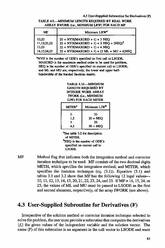
4.3 User-Supplied Subroutine for Derivatives (F') TABLE 49.-MINIMUM LENGTH REQUIRED BY REAL WORK
ARRAY RWORK (i.e., MINIMUM UW) FOR EACH MF
I MF I Minimum LRW' I I020 11,12,21,22 13,23 14,152425
2O+NYH(MAXORD+1)+3NEQ 22 + NYH(MAX0RD + 1 ) + 3 NEQ + (NEWz 22 + NYH(MAX0RD + 1) + 4 NEQ 22 + "(WORD + 1) + (2 ML + Mu + 4)NEQ
~~
'NYH is the number of ODE'S specifid on first call to LSODE. W O R D is the maximum method orda to be used for problem. NEQ is the number of ODE's specified on cumnt call to LSODE, and ML and MU are. resptively, the lower and upper half- bandwidths of the baaded Jrobian matrix.
TABLE 4.IO.-hUNIMUM LENGTH REQUIRED BY INTEGER WORK ARRAY WORK (is., MINIMUM LIW) FOR EACH MITER
MITER' I MinimumLmb
:,2 I 20
4.5 2O+NEQ
'Sce table 3.2 for description
G Q z i number of ODE'S specified on cumnt call to LSODE.
MF Method flag that indicates both the integration method and corrector iteration technique to be used. MF consists of the two decimal digits METH, which specifies the integration method, and MITER, which specifies the iteration technique (eq. (3.1)). Equation (3.1) and tables 3.1 and 3.2 show that MF has the following 12 legal values- 10,11,12,13,14,15,20,21,22,23,24,and25. IfMF=14,15,24,or 25, the values of ML and MLT must be passed to LSODE as the first and second elements, respectively, of the array WORK (see above).
4.3 User-Supplied Subroutine for Derivatives (F)
Irrespective of the solution method or corrector iteration technique selected to solve the problem, the user must provide a subroutine that computes the derivatives cf} for given values of the independent variable and the solution vector. The name Q of this subroutine is an argument in the call vector to LSODE and must
83
4. Description of Code Usage
therefore be declared EXTERNAL in the subprogram calling LSODE. The derivative subroutine F should have the form
SUBROUTINE F (NEQ, T, Y, YDOT) DIMENSION Y( I), YDOT( 1) in FORTRAN 66 or DIMENSION Y(*), YDOT(*) in FORTRAN 77
In addition, if NEQ is an array, the subroutine F should include a DIMENSION statement for it. The routine F should not alter the values in T, NEQ (or NEQ(l), if NEQ is an array), or the first N elements in Y, where N is the current number of ODE’S to be solved. The derivative vector should be returned in the array YDOT, with YDOT(1) = dyi/d5 (i = I), evaluated at 5 = T, y = Y.
If the calculation of ~} involves intermediate quantities whose current values, that is, at 5 = cn (or co,J, are required externally to LSODE, a special calculation, such as a call to the routine F, must be made. The results of the last call from the package to the routine F should not be used because they correspond to a Y value that is different from [or X(5,,J] and a 5 value that may be different from 5, (or &ut). Here tn is the independent variable value to which the numerical solution was advanced on the previous integration step and hut = TOUT. If a special call to subroutine F is made, to reduce the storage requirement, the YDOT argument may be replaced with RWORK(LSAVF), the base address of an N-dimensional array, SAVF (see table 3.8), used for temporary storage by LSODE; LSAVF is the 224th word (6th integer word after 218 real words) in the common block LSOOOl (table 3.6). If the derivative gn is required, it can be obtained by calling subroutine INTDY, as explained in section 4.8.
4.4 User-Supplied Subroutine for Analytical Jacobian (JAC)
If the corrector iteration technique selected by the user requires a Jacobian matrix, we recommend that a routine that computes an analytical Jacobian be provided. The name (JAC) of this routine is an argument in the call vector to LSODE and must therefore be declared EXTERNAL in the subprogram calling LSODE. The Jacobian subroutine JAC should have the form
SUBROUTINE JAC (NEQ, T, Y, ML, MU, PD, NROWPD) DIMENSION Y( 1), PD (NROWPD, 1) in FORTRAN 66 DIMENSION Ye), PD (NROWPD, *) in FORTRAN 77
Here ML and MU are, respectively, the (user-supplied) lower and upper half- bandwidths of the Jacobian matrix if it is banded; and NROWPD, which is set by
84
4.5 Detailed Usage Notes
the code, is the number of rows of the Jacobian matrix PD. For a banded matrix NROWPD is equal to the extended bandwidth (= 2ML + MU + l), and for a full matrix it is equal to the current number N of ODE's. If NEQ is an array, the subprogram JAC must include a DIMENSION statement for it.
This routine should not alter the values in NEQ (or NEQ(l), if NEQ is an array), T, ML, MU, or NROWPD. However, the Y array may, if necessary, be altered. For a full Jacobian matrix (MITER = 1) the element PD(I,J) (I = l,...,N, J = 1, ...,N) must be loaded with a&/ayi g=T;y=Y i = k j = J). In this case the
arguments ML and MU are not needed. If the Jacobian matrix is banded (MITER = 4), the element aJ/ayj (i = 1, ..., N, i -ML sj i + MU) must be loaded into PD (I - J + MU + 1, J) (I = i; J = j). Thus each band of the Jacobian matrix must be loaded in column-wise manner, with diagonal lines of J, from the top down, loaded into the rows of PD. For a diagonal matrix ML =MU = 0, and the diagonal elements must be loaded into a single row of length N. In any case the solver sets all elements of PD equal to zero before calling JAC, so that only the nonzero elements need to be loaded. Also each call to subroutine JAC is preceded by a call to subroutine F with the same arguments NEQ, T, and Y To improve computational efficiency, intermediate quantities needed by both routines may be saved by routine F in a common block, thereby avoiding recomputation by routine JAC. If necessary, even the derivatives at T can be accessed by JAC by means of this method.
If functional iteration (MITER = 0) or an internally generated Jacobian matrix (MITER = 2, 3, or 5) is used, a dummy version of JAC may nonetheless be required to satisfy the loader. This version may be given simply as follows:
I - (
SUBROUTINE JAC (NEQ, T, Y, ML, MU, PD, NROWPD) RE= END
4.5 Detailed Usage Notes
It is apparent from the description of the call sequence to LSODE that the code has many capabilities and therefore requires the user to set values for several parameters. To further clarify code usage and assist in selecting values for user- set parameters, we provide here a somewhat detailed guide. We first summarize how we expect the code to be normally used and then give detailed usage notes. Additional insight into code usage can be obtained from the discussions by Byrne and Hindmarsh (ref. 17), who examined in some detail the solution of 10 example problems representing a variety of problem types, and by Radhakrishnan (ref. 37), who studied the effects of various user-set parameters on the solution of stiff ODE's arising in combustion chemistry.
85
4. Description of Code Usage
4.5.1 Normal Usage Mode
The normal mode of communication with LSODE may be summarized as follows:
(1) Set initial values in Y. (2) Set NEQ, T, ITOL, RTOL, ATOL, LRW, LIW, and ME (3) Set TOUT = first output station, ITASK = 1, ISTATE = 1 , and IOPT = 0. (4) Call LSODE. (5) Exit if ISTATE < 0. (6) Do desired output of Y. (7) Exit if problem is finished. (8) Reset TOUT to next print station and return to step (4).
This procedure will result in LSODE (a) computing the step size to be attempted on the first step, (b) continuing the integration with step sizes generated internally until the first internal mesh point at or, more usually, just beyond TOUT, and (c) computing the solution at TOUT by interpolation. The returned value T will be set equal to TOUT exactly, and Y will contain the solution at TOUT. Because the normal output value of ISTATE is 2, it does not have to be reset for normal continuation.
4.5.2 Use of Other Options
The calling subprogram may also make use of other options included in the package. For example, in step (8) ISTATE could be reset to 3 to indicate that at TOUT some parameters, such as NEQ or MF, have been changed. The task to be performed, indicated by the value of ITASK, can, however, be changed without resetting ISTATE. In the event of integration difficulties parameter values may also be changed in step (3, followed by a return to step (4), if the new values will prevent a recurrence of the indicated trouble.
4.5.3 Dimensioning Variables
Irrespective of the options selected, the subprogram calling LSODE must include DIMENSION statements for all call sequence variables that are arrays. Such variables include Y, RTOL, ATOL, RWORK, IWORK, and, as discussed below, possibly NEQ. The solution vector Y may be declared to be of length NEQ or greater. The first NEQ elements of the Y array must be the variables whose ODE’S are to be solved. The remaining locations, if any, may be used to store other real data to be passed to the routines F and/or JAC. The LSODE package accesses only the first NEQ elements of Y the remaining elements are unchanged by the code.
The parameter NEQ is usually a scalar quantity. However, an array NEQ may
86
4.5 Detailed Usage Notes be used to store and pass integer data to the routines F and/or JAC. In this case the first element of NEQ must be set equal to the number of ODE’S. The LSODE package accesses only NEQ(1). However, NEQ is used as an argument in the calls to the routines F and JAC, so that these routines, and the MAIN program, must include NEQ in a DIMENSION statement.
4.5.4 Decreasing the Number of Differential Equations (NEQ)
In the course of solving a problem the user may decrease (but not increase) the number of ODE’s. This option is useful if some variables reach steady-state values while others are still varying. Dropping these constant quantities from the ODE list decreases the size of the system and hence increases computational efficiency. To use this option, upon return from LSODE at the appropriate time, the calling subprogram must reset the value of NEQ (or NEQ( 1)); set ISTATE = 3; reset the values of all other parameters that are either required to continue the integration, such as TOUT if ITASK = 1,3, or 4 (table 4.1), or are changed at the user’s option; and then call LSODE again. If the Jacobian matrix is declared to be banded (MITER = 4 or 5, table 3.2) and reductions can be made to the half- bandwidths ML and Mu, they will also produce efficiency increases. The option of decreasing the number of ODE’s may be exercised as often as the user .wishes. Of course, each time the size of the ODE system is decreased the changes discussed above should be made and the resulting number of ODE’s can never be less than 1. However, the LRW and LIW values need not be reset.
If, at any time, the number of ODE’S is decreased from N to N’, LSODE will drop the last N - N’ ODE’S from the system and integrate the first N‘equations. It is therefore important in formulating the problem to order the variables carefully and make sure that it is indeed the last N - N’ variables that attain steady-state values. In continuing the integration LSODE will access only the first N’ elements of Y However, the remaining N - N‘, or more, elements can be accessed by the user, and so no special programming is needed in either routine F or JAC.
4.5.5 Specification of Output Station (TOUT)
The argument TOUT must be reset every time LSODE is called if the option given by ITASK = 1 , 3, or 4 is selected. For the other two values of ITASK (Le., 2 and 5), TOUT need be set only on the first call to LSODE. Irrespective of the value of ITASK, the TOUT value provided on the first call to LSODE is used to determine the direction of integration and, if the user has not supplied a value for it, to compute the step size to be attempted on the first step. Therefore unless the user specifies the value for the initial step size, it is recommended that some thought be given to the value used for TOUT on the first call to LSODE.
On the first call to LSODE, that is, with ISTATE = 1, TOUT may be set equal to the initial value of the independent variable. In this case LSODE will do nothing, and so the value ISTATE = 1 will be returned to the calling subprogram; however,
87
4. Description of Code Usage
an internal counter will be updated to prevent repeated calls of this nature. If such a “first” call is made more than four times in a row, an error message will be issued and the execution terminated.
On the second and subsequent calls to LSODE there is no requirement that the TOUT values be monotonic. However, a value for TOUT that “backs up” is limited to the current internal interval [(TCUR - HU),TCUR], where TCUR is the current value of the independent variable and HU is the step size used on the previous step.
4.5.6 Specification of Critical Stopping Point (TCRIT)
In addition to TOUT a value must be specified for TCRIT if the option ITASK = 4 is selected. TCRIT may be equal to TOUT or beyond it, but not behind it, in the direction of integration. The integration is not permitted to overshoot TCRIT, so that the option is useful if, for example, a singularity exists at or beyond TCRIT. This variable is also required with the option ITASK = 5. In either case the first element of the array RWORK (i.e., RWORK( 1)) must be set equal to TCRIT. If the solver reaches TCRIT within roundoff, it will return T = TCRIT exactly and the solution at TCRIT is returned in Y. To continue integrating beyond TCRIT, the user must reset either ITASK or TCEUT. In either case the value of ISTATE need not be reset. However, whenever TCRIT is changed, the new value must be loaded into RWORK(1).
4.5.7 Selection of Local Error Control Parameters (ITOL, RTOL, and ATOL)
Careful thought should be given to the choice of ITOL, which together with RTOL and ATOL determines the nature of the error control performed by LSODE. The value of ITOL dictates the value of the local error weight vector m, with element EWTj defined as
EWT~ = RTOL,~~~+ATOL, , (4.1)
where RTOLj and ATOL, are, respectively, the local relative and absolute error tolerances for the ith solution component Yj and the bars 1.1 denote absolute value. The solver controls the estimated local errors {d i} in { Yi] by requiring the root- mean-square (rms) norm of dj/EWTj to be 1 or less.
Pure relative error control for the ith solution component is obtained by setting ATOL, = 0; RTOLi is then a measure of the number of accurate significant fig- ures in the numerical solution. This error control is generally appropriate when widely varying orders of magnitude in Yj are expected. However, it cannot be used if the solution vanishes because relative error is then undefined. Pure absolute error control for the ith solution component is obtained by setting
88
4.5 Detailed Usage Notes RTOLi = 0; ATOLi is then a measure of the largest number that may be neglected.
Both RTOL and ATOL can be specified (1) as scalars, so that the same error tolerances are used for all variables, or (2) as arrays, so that different tolerances are used for different variables. The value of the user-supplied parameter ITOL indicates whether RTOL and M O L are scalars or arrays. The legal values that
-can be assigned to ITOL and the corresponding types of RTOL and M O L are given in table 4.2. If RTOL and/or ATOL are arrays, the calling subprogram must include an appropriate DIMENSION statement. A scalar RTOL is generally appropriate if the same number of significant figures is acceptable for all components of Y. A scalar ATOL is generally appropriate when all components of Y, or at least their peak values, are expected to be of the same magnitude.
In addition to ITOL, RTOL and ATOL should be selected with care. Now the code controls an estimate of only the local error, that is, an estimate of the error committed on taking a single step, starting with data regarded as exact. However, what is of interest to the user is the global truncation error or the actual deviation of the numerical solution from the exact solution. This error accumulates in a nontrivial manner from the local errors and is neither measured nor controlled by the code. It is therefore recommended that the user be conservative in choosing values for the local error tolerance parameters. However, requesting too much accuracy for the precision of the machine will result in an error exit (table 4.4). In such an event the minimum factor TOLSF by which RTOL and ATOL should both be scaled up is returned by LSODE (see table 4.7). Some experimentation may be necessary to optimize the tolerance parameters, that is, to determine values that produce sufficiently accurate solutions while minimizing the execution time. The global errors in solutions generated with particular values for the local error tolerance parameters can be estimated by comparing them with results produced with smaller tolerances. In reducing the tolerances all components of RTOL and ATOL, and hence of EwT, should be scaled down uniformly.
There is no requirement that the same values for ITOL, RTOL, and ATOL be used throughout the problem. If during the course of the problem any of these parameters is changed, the user should reset ISTATE = 3 before calling LSODE again. (ISTATE need not be reset; however, LSODE will not then check the legality of the new values.) This option is useful, for example, if the solution displays rapid changes in a small subinterval but is relatively smooth elsewhere. To accurately track the solution in the rapidly varying region, small values of RTOL and ATOL may be required. However, in the smooth regions these tolerances could be increased to minimize execution time.
4.5.8 Selection of Integration and Corrector Iteration Methods (MF)
The choice of the method flag MF may also require some experimentation. The user should consider the nature of the problem and storage requirements. The primary consideration regarding MF is stiffness. If the problem is not stiff, the best choice is probably MF = 10 (Adams-Moulton (AM) method with functional
89
4. Description of Code Usage
iteration.) If the problem is stiff to a significant degree, METH should be set equal to 2 (table 3.1), and MITER (table 3.2) depends on the structure of the Jacobian matrix. If the Jacobian is banded, MITER = 4 (user-supplied analytical Jacobian) or 5 (internally generated Jacobian by finite-difference approximations) should be used. For either of these two MITER values the user must set values for the lower (ML) and upper (MU) half-bandwidths of the Jacobian matrix. The first and second elements of the integer work array IWORK must be set equal to ML and MU, respectively; that is, IWORK( 1) = ML and IWORK(2) = MU. For a full matrix MITER should be set equal to 1 (analytical Jacobian) or 2 (internally generated Jacobian). If the matrix is significantly diagonally dominant, the choice MITER = 3, that is, Jacobi-Newton (JN) iteration using an internally generated diagonal approximation for the Jacobian matrix, can be made. To use this iteration technique with an analytical Jacobian, set MITER = 4 and ML = MU = 0.
If the problem is only mildly stiff, the choice METH = 1 (Le., the AM method) may be more efficient than METH = 2 (i.e., the backward differentiation formula (BDF) method). For this case experimentation would be necessary to identify the optimal METH. If the user has no a priori knowledge regarding the stiffness of the problem, one way to determine its nature is to try MF = 10 and examine the behavior of both the solution and step size pattern. (It is recommended that some upper limit be set for the total number of steps or derivative evaluations to avoid excessive run times.) If the typical values of the step size are much smaller than the solution behavior would appear to require, for example, more than 100 steps are taken over an interval in which the solution changes by less than 1 percent, the problem is probably stiff. The degree of stiffness can be estimated from the step sizes used and the smoothness of the solution.
Irrespective of the integration method selected, the least effective iteration technique is functional iteration, given by MITER = 0, and the most effective is Newton-Raphson (NR), given by MITER = 1 or 2 (4 or 5 for a banded Jacobian matrix). Generally JN iteration is somewhere in between. However, storage requirements increase in the same order as the effectiveness of the iteration technique (see table 4.9), and so trade-off considerations are necessary. For reasons of computational efficiency the user is encouraged to provide a routine for computing the analytical Jacobian, unless the system is fairly complicated and analytical expressions cannot be derived for the matrix elements. The accuracy of the Jacobian calculation can be checked by comparison with the J internally generated with MITER = 2 or 5. Jacobi-Newton iteration requires considerably less storage and execution time per iteration but will be effective only if the Jacobian matrix is significantly diagonally dominant.
The importance of supplying an analytical Jacobian matrix, especially for large problems, is illustrated by Radhakrishnan (ref. 37), who studied 12 test problems from combustion kinetics. The problems covered a wide range of reaction conditions and reaction mechanism size. The effects on solution efficiency of (1) METH, (2) the first output station, and (3) optimizing the local error tolerances were also examined.
90
4.6 Optional Input
4.5.9 Switching Integration and Corrector Iteration Methods
The user may specify different values for MF in different subintervals of the problem. This option is useful if the problem changes character and is nonstiff in some regions and stiff elsewhere. Because stiff problems are usually characterized by a nonstiff initial “transient” region, one could use MF = 10 in the initial region and then switch to MF = 21 (the BDF method with NR iteration using an analytical Jacobian matrix) in the later stiff regime. It is very straightfoiward to change integration methods and corrector iteration techniques. Upon return from LSODE the user simply resets MF to the desired new value. The other action required is to reset ISTATE = 3 before calling LSODE again. The lengths LRW and LIW, respectively, of the arrays RWORK and IWORK depend on MF (see tables 4.9 and 4.10). If different methods are to be used in the course of solving a problem, storage corresponding to at least the maximum values of LRW and LIW must be allocated. That is, the dimensions of RWORK and IWORK must be set equal to at least the largest of the LRW and LIW values, respectively, required by the different methods to be used.
4.6 Optional Input
In addition to the input parameters whose values are required by the code, the user can set values for several other Parameters to control both the integration and the output from the code. These optional input parameters are given in table 4.6, together with their locations and default values. If any of these parameters are used, the user must set IOPT = 1 to relay this information to the solver, which will examine all optional input parameters and select only those for which nonzero values are specified. A value of zero for any parameter will cause its default value to be used. Thus to use a subset of the optional inputs, set RWORKO = 0.0 and IWORKO = 0 (I = 5 to 7), and then set parameters of interest to the desired (nonzero) values. The variable HO, the step size to be attempted on the first step, must indicate the direction of integration. That is, HO must be a positive quantity for integration in the forward direction (increasing values of the independent variable) and negative otherwise. All other input parameters must be positive numbers; otherwise, an error exit will occur.
To reset any optional input parameter on a subsequent call to LSODE, ISTATE must be set equal to 3. IOPT is not altered by LSODE and therefore need not be reset. Also because the code does not alter the values in RWORK (5) to RWORK (7) and IWORK(5) to IWORK(7), only parameters for which new values are required need to be reset. To specify a default value for any parameter for which a nondefault value had previously been used, simply load the appropriate location in RWORK or IWORK with a zero. Of course, if all variables are to have default values, simply reset IOPT = 0.
91
4. Description of Code Usage
4.6.1 Initial Step Size (HO)
The sign of the step size HO must agree with the direction of integration; otherwise, an error exit will occur. Also, its magnitude should be considerably smaller than the average value expected for the problem because the code starts the integration with a first-order method. Of course, the integrator tests that the given step size does produce a solution that satisfies the local error test and, if necessary, decreases it (in magnitude). The only test made on the magnitude of HO prior to taking the first step is that it does not exceed the user-supplied value for HMAX, the maximum absolute step size allowed for the problem.
4.6.2 Maximum Step Size (HMAX)
The user may have to specify a finite value for HMAX (default value, -) if the solution is characterized by rapidly varying transients between long smooth regions. If the step size is too large, the solver may skip over the fine detail that the user may be (primarily) interested in. An example of this behavior is the buildup of ozone and oxygen atom concentrations in the presence of sunlight (ref. 17).
4.6.3 Maximum Method Order (MAXORD)
The optional input parameter MAXORD, the maximum method order to be attempted on any step, should not exceed the default value-12 for the AM method and 5 for the BDF method. If it does, it will be reduced to the default value. Also, in the course of solving the problem, if MAXORD is decreased to a value less than the current method order, the latter quantity will be reduced to the new MAXORD.
The maximum method order has to be restricted to a value less than the default value for stiff problems when the eigenvalues of the Jacobian matrix are close to the imaginary axis; that is, the solution is highly oscillatory. In such a situation the BDF method of high order (2 3) has poor stability characteristics and, as the stability plots in Gear (ref. 10) show, the unstable region grows as the order is increased. For this reason MAXORD should be set equal to 3 unless the eigenvalues are imaginary; that is, Re&) = 0 and Im(hi) # 0, where Re&) and Im(hi) are the real and imaginary parts of hi, the ith eigenvalue. In this case the value MAXORD = 2 should be used.
4.7 Optional Output
The user is usually primarily interested in the numerical solution and the corresponding value of the independent variable. These quantities are always returned in the call variables Y and T. In addition, several optional output
92
4.8. Other Routines
quantities that contain information about the integration are returned by LSODE. These quantitites are given in tables 4.7 and 4.8, together with their locations. Some of these quantities give a measure of the computational work required and may, for example, help the user decide if the problem is stiff or if the right method is being used. Other output quantities will, in the event of an error exit, help the user either set legal values for some parameters or identify the reason for repeated convergence failures or local error test failures.
4.8 Other Routines
To gain additional capabilities, the user can access the following subroutines included in the LSODE package: INTDY, SRCOM, XSETF, and XSETUN. Among these, only INTDY is used by LSODE.
4.8.1 Interpolation Routine (Subroutine INTDY)
The subroutine INTDY provides derivatives of Y, up to the current order, at a specified point T and may be called only after a successful return from LSODE. The call to this routine takes the form
CALL INTDY (T, K, RWORK(21), NYH, DKY, FLAG)
where T, K, RWORK(21), and NYH are input parameters and DKY and FLAG are output parameters. The arguments to lNTDY are defined as follows:
T
K
RWORK(2 1)
NYH
Value of independent variable at which the results are required. For the results to be valid T must lie in the interval [(TCUR - HU),TCUR], where TCUR and HU are defined in table 4.7.
Integer that specifies the desired derivative order and must satisfy 0 I K I current method order NQCUR (see table 4.7 for location of this quantity). Now, because the method order is never less than 1, the first derivative a/& can always be obtained by calling INTDY.
Base address of the Nordsieck history array (see table 4.8).
Number of ODE's used on the first call to LSODE. If the number of ODE's is decreased during the course of the problem, NYH should be saved. An alternative way of obtaining NYH is to include the common block LSOOOl in the subprogram calling INTDY. LSODE saves NYH in LSOOOl as the 232nd word-the 14th integer word after 218 real words (see table 3.6).
93
4. Description of Code Usage
DKY Array of length N that contains the Kth derivative of Y at T. The subprogram calling INTDY must include a DIMENSION statement for DKY if NYH > 1. Alternatively, to save storage, DKY can be replaced with RWORK(LSAVF)-see section 4.3.
IFLAG An error flag with following values and meanings: 0
-1 -2
Both T and K were legal. Illegal value was specified for K. Illegal value was specified for T.
4.8.2 Using Restart Capability (Subroutine SRCOM)
The subroutine SRCOM is useful if one is either alternating between two or more problems being solved by LSODE or interested in interrupting a run and restarting it later. The latter situation may arise, for example, if one is interested in steady-state values with no a priori knowledge of the required integration interval. The run may be stopped periodically, the results examined and, if necessary, the integration continued. This procedure is clearly more economical than making repeated runs on the same problem with, say, increasing values of TOUT. To exploit the capability of stopping and then continuing the integration, the user must save and then restore the contents of the common blocks LSOOOl and EHOOO1. This information can be stored and restored by calling SRCOM. The call to this routine takes the form
CALL SRCOM (RSAV, ISAV, JOB)
where RSAV must be declared as a real array of length 2 18 or more in the calling subprogram and ISAV as an integer array of length 41 or more and JOB is an integer flag whose value (= 1 or 2) indicates the action to be performed by SRCOM as follows: JOB = 1 means “save the contents of the two common blocks,’’ and JOB = 2 means “restore this information.”
Thus to store the contents of EHOOOl and LSOOOl, SRCOM should be called as follows:
CALL SRCOM (RSAV, ISAV, 1)
Upon return from SRCOM, RSAV and ISAV will contain, respectively, the 21 8 real and 39 integer words that together make up the common block LSOOOl. The 40th and 41st elements of ISAV will contain the two integer words MESFLG and LUNIT in the common block EHOOOl (table 3.6). The lengths and contents of the arrays RWORK and WORK must also be saved. The lengths LENRW and LENIW required for the arrays RWORK and IWORK are saved by LSODE as the 17th and 18th elements, respectively, of the array IWORK (see table 4.7).
To continue the integration, the arrays RWORK and IWORK and the contents of the common blocks LSOOOl and EHOOOl must be restored. The common block
94
4.9 Optionally Replaceable Routines
contents are restored by using the previously saved arrays RSAV and ISAV and calling the routine SRCOM as follows:
CALL SRCOM (RSAV, ISAV, 2)
The user should then set values for the input parameters required by LSODE, and the integration can be continued by calling this routine. Note, in particular, that ISTATE must be set equal to 2 or 3 to inform LSODE that the present call is a continuation one for the problem (see table 4.3).
4.8.3 Error Message Control (Subroutines XSETF and XSE")
To reset the value of the logical unit number LuNlT for output of messages from the code, the routine XSETUN should be called as follows:
CALL XSETUN (LUN)
where LUN is the new value for LUNIT. Action is taken only if the specified value is greater than zero.
The value of the flag MESFLG, which controls whether messages from the code are printed or not, may be reset by calling subroutine XSETF as follows:
CALL XSETF (MFLAG)
where MFLAG is the new value for MESFLG. The legal values for MFLAG are 0 and 1. Specifying any other value will result in no change to the current value of MESFLG. Setting MFXAG = 0 does carry the risk of losing valuable information through error messages from the integrator.
4.9 Optionally Replaceable Routines
If none of the error control options included in the code are suitable, more general error controls can be obtained by substituting user-supplied versions of the routines EWSET and/or WORM (table 3.3). Both routines are concerned with measuring the local error. Hence any replacement may have a major impact on the performance of the code. We therefore recommend that modifications be made only if absolutely necessary, and that too with great caution. Also the effect of the changes and the accuracy of the programming should be studied on some simple problems.
4.9.1 Setting Error Weights (Subroutine EWSET)
The subroutine EWSET sets the array of error weights EWT, equation (4.1). This routine takes the form
95
4. Description of Code Usage
SUBROUTINE EWSET (N, ITOL, RTOL, ATOL, YH, EWT)
where N is the current value of the number of ODE’S; ITOL, RTOL, ATOL, and EWT have been defined previously; and YH contains the current Nordsieck history array, that is, the current solution vector YCUR and its NQ scaled derivatives, where NQ is the current method order. On the first call to EWSET from the routine LSODE, YCUR is the same as the Y array (which then contains the initial values supplied by the user); thereafter the two arrays may be different.
The error weights {EWTi} are used in the local truncation error test, which requires that the rms norm of diEWT, be 1 or less. Here, di is the estimated local error in Yi. The above norm is computed in the routine VNORM (discussed in section 4.9.2) to which the EWT array is passed.
If the user replaces the current version of EWSET, the new version must return in each EWTi (i = 1 ,..., N) a positive quantity for comparison with di. This routine is called by the routine LSODE only (tables 3.4 and 3.5). However, in addition to its use in the local truncation error test (which is performed in the routine STODE), EWT is used (1) by the routine LSODE in computing the initial step size HO and the optional output integer IMXER (table 4.7) and (2) by the routine PREPJ in computing the increments in solution vector for the difference quotient Jacobian matrix (MITER = 2 or 5, table 3.2) and for the diagonal approximation to the Jacobian matrix (MITER = 3). The base address for EWT in the array RWORK is LEWT, which is the 222nd word (the 4th integer word after 218 real words) in the common block LSOOOl .
If the user’s version of EWSET uses current values of the derivatives of Y, they can be obtained from YH, as described later. Indeed, derivatives of any order, up to NQ, can be found from YH, whose base address in RWORK is LYH (= 21), the 221st word (the 3rd integer word past 21 8 real words) in LSOOOl. The array YH is of length NYH(NQ + l), where NYH is the value of N on the first call to LSODE. The first N elements correspond exactly to the YCUR array. The remaining terms contain scaled derivatives of YCUR. For example, the N elements J*NYH + 1 to J*NYH + N (J = O,l, ..., NQ) contain the Jth scaled derivative HJyCJ)/J!, where H is the current value of the step size. On the first call to EWSET, before any integration is done, H is (temporarily) set equal to 1 .O. Thereafter its value may be determined from LSOOO1, where it is the 212th real word. This common block also contains NYH as the 232nd word (the 14th integer word past 218 real words) and NQ as the 253rd word (the 35th integer word past 21 8 real words). Thus if the user wishes to use the Jth derivative in EWSET, it may be obtained by including the following statements:
SUBROUTINE EWSET (N, ..., YH, ..., EWT) REAL (or DOUBLE PRECISION) YH, EWT, RLS, H, ... INTEGER N, ILS, NQ, NYH, ... DIMENSION YH( l), EWT(I), ... in FORTRAN 66 DIMENSION YH(*),EWT(*), ... in FORTRAN 77
96
4.9 Optionally Replaceable Routines
COMMON/LSOOO1/RLS(218), ILS(39) NQ=ILS(35) NYH = ILS(14) H = RLS(212)
The Jth derivative (0 5 J 5 NQ) is then given by
J! YH(J*NYH+I) yp = , I=l , ..., N,
HJ
where Yinis the Jth derivative of YI. The routine must include a data type declaration and a DIMENSION statement for 2n. To save on storage, these values may be stored temporarily in the vector EWT.
4.9.2 Vector-Norm Computation (Function VNORM)
The real (or double precision) function routine VNORM computes the weighted - root-mean-square (rms) norm of a vector. It is used as follows:
where N is the length of the real arrays V, which contains the vector, and W, which contains the weights. Upon return from VNORM, D contains the weighted rms- norm
This routine is used by STODE to compute the weighted rms norm of the estimated local error. STODE also uses information returned by WORM to perform the corrector convergence test and to compute factors that determine if the method order should be changed. Other routines that access WORM are LSODE, to compute the initial step size HO, and PREPJ, to compute the increments in the solution vector for generating difference quotient Jacobians (MITER = 2 or 5, table 3.2).
If the user replaces the routine VNORM, the new version must return a positive quantity in VNORM, suitable for use in local error and convergence testing. The weight array W can be used as needed, but it must not be altered in WORM. For example, the max-norm, that is, maxlVflj, satisfies this requirement, as does a n o m that ignores some components of V. The latter procedure has the effect of suppressing error control on the corresponding components of 1.
97
4. Description of Code Usage
4.10 Overlay Situation
If LSODE is to be used in an overlay situation, the user must declare the variables in the call sequence to LSODE and in the two internal common blocks LSOOOl and EHOOOI in the MAIN program to ensure that their contents are preserved. The common block LSOOOl is of length 257 (218 real or double- precision words followed by 39 integer words), and EHOOOI contains two integer words (see table 3.6).
4.11 Troubleshooting
In this section we present a brief discussion of the corrective actions that may be taken in case of difficulty with the code. If the execution is terminated prematurely, the user should examine the error message and the value of ISTATE returned by LSODE (table 4.4). We therefore recommend that the current value of MESFLG not be changed, at least until the user has gained some experience with the code. The legality of every input parameter, both required and optional, is checked. If illegal input is detected by the code, it returns to the calling subprogram with ISTATE = -3. The error message will be detailed and will make clear what corrective actions to take. If the illegal input is caused by a request for too much accuracy, the user should examine the value of TOLSF returned in RWORK( 13) (table 4.7) and make necessary adjustments to RTOL and ATOL, as described in section 4.5.7. If an excessive accuracy requirement is detected during the course of solving the problem, the value ISTATE = -2 is returned. To continue the integration, make the adjustments mentioned above, set ISTATE = 3, and call LSODE again.
Another difficulty related to accuracy control may be encountered if pure relative error control for, say, the ith variable is specified (Le., ATOLj = 0). If this solution component vanishes, the error test cannot be applied. In this situation the value ISTATE = -6 is returned to the calling subprogram. The error message identifies the component causing the difficulty. To continue integrating, reset ATOL for this component to a nonzero value, set ISTATE = 3, and call LSODE again.
If more than MXSTEP (default value, 500) integration steps are taken on a single call to LSODE without completing the task, the error return ISTATE = -1 is made. The problem might be the use of an inappropriate integration method or iteration technique. The use of MF = 10 (or 20) on a stiff problem is one example. The user should, as described previously under the selection of MF (section 4.5.8), verify that the value of MF is right for the problem. Very stringent accuracy requirements may also cause this difficulty. Another possibility is that pure relative error control has been specified but most, or all, of the 1x1 are very small but nonzero. Finally, the solution may be varying very rapidly, forcing the integrator to select very small step sizes, or the integration interval may be very
98
4.U Troubleshooting
long relative to the average step size. To continue the integration, simply reset ISTATE = 2 and call LSODE again-the excess step counter will be reset to zero. To prevent a recurrence of the error, the value of MXSTEP can be increased, as described in section 4.6. If this action is taken between calls to LSODE, ISTATE must be set equal to 3 before LSODE is called again. Irrespective of when MXSTEP is increased, IOPT should be set equal to 1 before the next call to LSODE.
If the integrator encounters either repeated local error test failures or any local error test failure with a step size equal to the user-supplied minimum value HMIN (table 4.6), LSODE returns with ISTATE = -4. The difficulty could be caused by a singularity in the problem or by inappropriate input. The user should check subroutines F and JAC for errors. If none is found, it may be necessary to monitor intermediate quantities. The component IMXER causing the error test failure is returned as IWORK(16) (table4.7). The values Y(IMXER), RTOL(IMXER), ATOL-R), and ACOR(IMXER) (see table 4.8) should be examined. If pure relative error control had been specified for this component, very small but nonzero values of Y(IMXER) may cause the difficulty.
These checks should also be made if the integration fails because of either repeated corrector convergence test failures or any such failure with a step size equal to HMIN. In this case LSODE returns the value ISTATE = -5 along with a value for IMXER defined above. If an analytical Jacobian is being used, it should be checked for errors. The accuracy of the calculation can also be checked by comparing J with that generated internally. Another reason for this failure may be the use of an inappropriate MITER, for example, MITER = 3 for a problem that does not have a diagonally dominant Jacobian. It may be helpful to try different values for MITER and monitor the successive corrector estimates stored as the Y array in subroutine STODE.
In addition to the error messages just discussed, a warning message is printed if the step size H becomes so small that T + H = T on the computer, where T is the current value of the independent variable. This error is not considered fatal, and so the execution is not terminated nor is a return made to the calling subprogram. No action is required by the user. The warning message is printed a maximum number of MXHNIL (default value, 10) times per problem. The user can change the number of times the message is printed by resetting MXHNIL, as discussed in section 4.6. To indicate the change to LSODE, the parameter IOPT must be set equal to 1 before LSODE is called.
99

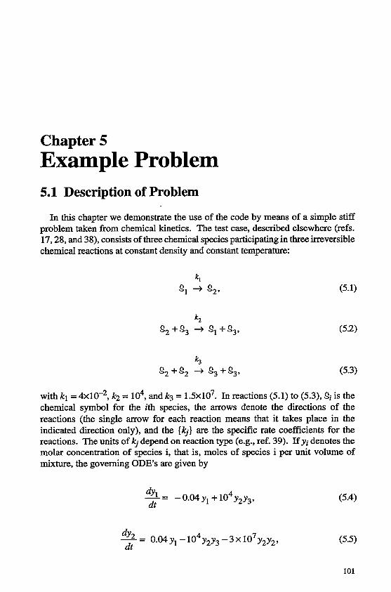
Chapter 5 Example Problem 5.1 Description of Problem
In this chapter we demonstrate the use of the code by means of a simple stiff problem taken from chemical kinetics. The test case, described elsewhere (refs. 17,28, and 38), consists of three chemical species participating in three irreversible chemical reactions at constant density and constant temperature:
kl
s, + 52,
k3 s2+s, -+ s3+s3,
with kl = 4 ~ 1 0 - ~ , k2 = lo4, and k3 = 1 . 5 ~ 1 0 ~ . In reactions (5.1) to (5.3), Si is the chemical symbol for the ith species, the arrows denote the directions of the reactions (the single arrow for each reaction means that it takes place in the indicated direction only), and the {kj} are the specific rate coefficients for the reactions. The units of kj depend on reaction type (e.g., ref. 39). If yi denotes the molar concentration of species i, that is, moles of species i per unit volume of mixture, the governing ODE’S are given by
* = - 0.04 y1 + 1 0 4 ~ ~ ~ ~ , dt (5-4)
%= 0 . 0 4 ~ ~ - 1 0 4 ~ ~ ~ ~ -3x10⁷y2y2, dt
101
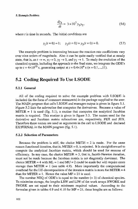
5. Example Problem
%= 3x10⁷y2y2, dt
where t is time in seconds. The initial conditions are
Y1(t=O)=l; ~ ~ ( r = O ) = ~ ~ ( t = 0 ) = 0 . (5.7)
The example problem is interesting because the reaction rate coefficients vary over nine orders of magnitude. Also it can be quite easily verified that at steady state, that is, as t + 00, y1+ 0, y2 + 0, and y3 + 1. To study the evolution of the chemical system, including the approach to the final state, we integrate the ODE’s up to t = 4 ~ 1 0 ’ ~ s , generating output at t = 0 . 4 ~ 1 r s (n = O,l, ..., 11).
5.2 Coding Required To Use LSODE
5.2.1 General
All of the coding required to solve the example problem with LSODE is included (in the form of comment statements) in the package supplied to the user. The MAIN program that calls LSODE and manages output is given in figure 5.1. Figure 5.2 lists the subroutine that computes the derivatives. Because a value of MITER = 1 is used (fig. 5.1), a routine that computes the analytical Jacobian matrix is required. This routine is given in figure 5.3. The names used for the derivative and Jacobian matrix subroutines are, respectively, FEX and JEX. Therefore these names are used as arguments in the call to LSODE and declared EXTERNAL in the MAIN program (fig. 5.1).
5.2.2 Selection of Parameters
Because the problem is stiff, the choice METH = 2 is made. For the same reason functional iteration, that is, MITER = 0, is rejected. It is straightforward to compute the analytical Jacobian matrix, which should be used for reasons of efficiency. In any case, the choice MITER = 3, that is, Jacobi-Newton iteration, must not be made because the Jacobian matrix is not diagonally dominant. The choice MITER = 4 with ML = 1 and MU = 2 could be made but will require more storage than MITER = 1 (see table 4.9). More importantly the computational overhead for the LU-decomposition of the iteration matrix is more for MITER = 4 than for MITER = 1. Hence the value MF = 21 is used.
The number NEQ of ODE’s is equal to the number (= 3) of chemical species. To minimize storage, the lengths LRW and LIW of the work arrays RWORK and IWORK are set equal to their minimum required values. According to the formulas given in tables 4.9 and 4.10 for MF = 21, these lengths are as follows:
102
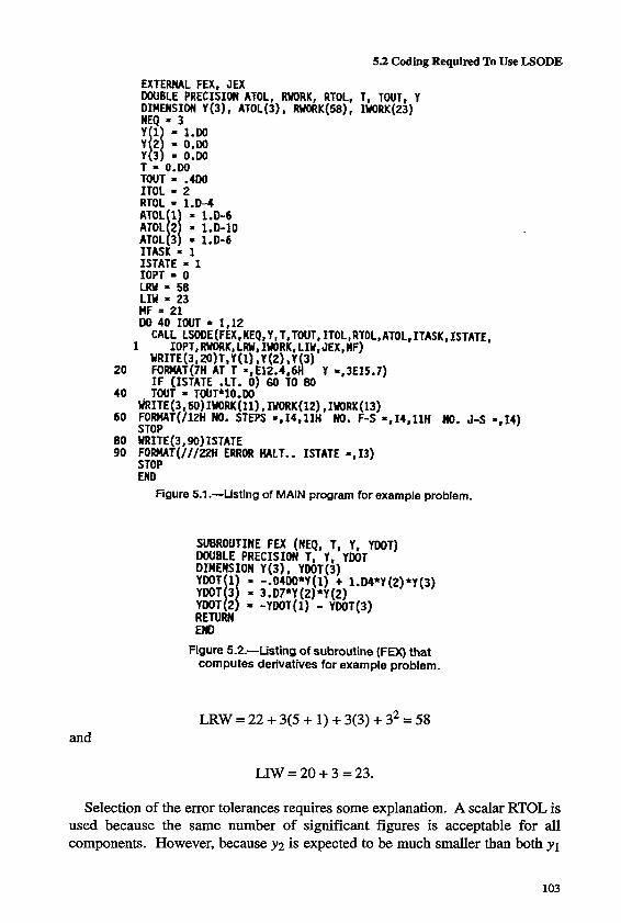
5.2 Coding Required To Use LSODE
EXTERNAL FEX, JEX DOUBLE PRECISION ATOL, RUORK, RTOL, T, TOUT, Y DIMENSION Y (3), ATOL(3), RYORK(58), IWRK(23) NEQ = 3
T - 0-W _ _ _ _ TOUT = .4W ITOL = 2 RTOL l.D-4
ITASK = 1 ISTATE = 1 IOPT - 0 m=58 L I Y - 23 MF = 21 00 40 IOUT = 1,12
CALL L!3DE(FEX,NEQ,Y,T,TWT, ITOL,RTOL,ATOl, ITASK,ISTATE, 1 IOPT, RWORK, LRV, IWRK, LIY, JEX,WF)
m I T E ( 3 1 a) T, Y(1) I r(2) a Y(3) 20 FOW(AT(7H AT T =,E12.4,6H Y =,3E15.7)
40 TOUT - TOUT*lO-W IF (ISTATE .LT. 0) 60 TO 80
~ I T E ( 3 , 6 O ) I W R K ( l l ) , IYORK(lZ), IYORK(13)
STnP 60 FORHAT(/lZH n0. STEPS =,14111H NO. F-S ~ 8 1 4 , l l H NO. J-S =,14)
80 GiTE(3,90) ISTATE 90 FOW(AT(///ZH ERROR HALT.. ISTATE -,IS)
STOP U I D
Figure 5.1 .-Listing of MAIN program for example problem.
SUBROUTINE FEX (NEQ, T, Y, YWT) WUBLE PRECISION T, Y, YDOT DIMENSION Y(3), YDoT(3) Y W T 1 YWT131 = J.D7*Y(Z)*Y(Z) YM)T 2 -YDOT(l) - YDOT(3) RETURN Em
computes derivatives for example problem.
a -.04DO*Y(1) + l.D4*Y(Z)*Y(3)
Figure 59.-Listing of subroutine (FEW that
LRW =22 + 3(5 + 1) + 3(3) + 32 = 58 and
LIW = 20 + 3 = 23.
Selection of the error tolerances requires some explanation. A scalar RTOL is used because the same number of significant figures is acceptable for all components. However, because y2 is expected to be much smaller than both y1
103
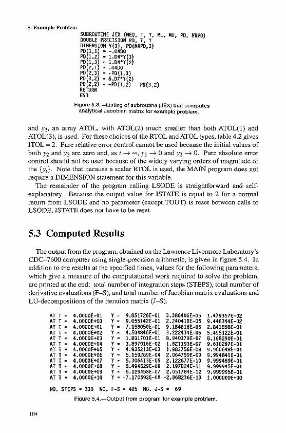
5. Example Problem SUBROUTINE JEX (NEQ, T, Y, ML, MU, PD, NRPD) DOUBLE PRECISION PD, TI Y DIHENSION Y(3), PD(WRPD.3) PD(1.1) -.04DO
RETURN END
1. D4*Y 3 1 .D4*Y 121 .04DO -PD( l , 3) 6.D7*Y (2) -PD(l,Z) -
Figure 5.3.-Listing of subroutine (JEX) that computes analytical Jacobian matrix for example problem.
and p3, an array ATOL, with ATOL(2) much smaller than both ATOL(1) and ATOL(3), is used. For these choices of the RTOL and ATOL types, table 4.2 gives ITOL = 2. Pure relative error control cannot be used because the initial values of both y2 and p3 are zero and, as t -+ 00, p1 -+ 0 and p2 -+ 0. Pure absolute error control should not be used because of the widely varying orders of magnitude of the {y , } . Note that because a scalar RTOL is used, the MAIN program does not require a DIMENSION statement for this variable.
The remainder of the program calling LSODE is straightforward and self- explanatory. Because the output value for ISTATE is equal to 2 for a normal return from LSODE and no parameter (except TOUT) is reset between calls to LSODE, ISTATE does not have to be reset.
5.3 Computed Results
The output from the program, obtained on the Lawrence Livermore Laboratory’s CDC-7600 computer using single-precision arithmetic, is given in figure 5.4. In addition to the results at the specified times, values for the following parameters, which give a measure of the computational work required to solve the problem, are printed at the end: total number of integration steps (STEPS), total number of derivative evaluations (F-S), and total number of Jacobian matrix evaluations and LU-decompositions of the iteration matrix (J-S).
AT T = AT T = AT T = AT T = AT T = AT T = AT T * AT T = AT T = AT T = AT T = AT T =
4.0000E-01 4.00OOE+OO 4.00OOE+Ol 4 .OOOOE+O2 4.0000E+03 4.0000E+04 4.0000E+05 4.0000E+06 4.0000E+07 4.0000E+08 4.0000E+09 4.0000E+10
Y = Y = Y = Y = Y = Y = Y - Y - Y = Y = Y = Y =
9.851726E-01 9.055142E-01 7.158050E-01 4.504846E-01 1.831701E-01 3.897016E-02 4.935213E-03 5.159269E-04 5.306413E-05 5.494529E-06 5.129458E-07
-7.170592E-08
3.386406E-05
9.184616E-06 3.222434E-06 8.940379E-07 1.621193E-07 1.983756E-08 2.064759E-09 2.122677E-10 2.197824E-11 2.051784E-12
-2.868236E-13
2. 2 4 ~ i a ~ - 0 5 1.479357E-02 9.446344E-02 2.841858E-01 5.49512ZE-01 8.168290E-01 9.610297E-01 9.950648E-01 9.994841E-01 9,999469E-01 9.999945E-01 9.999995E-01 1.000000E+00
NO. STEPS = 330 NO. F-S = 405 NO. J-S 69
Figure 5 .4 .4utput from program for example problem.
104
Chapter 6 Code Availability
The present version of LSODE, dated March 30, 1987, is available in single or double precision. The code has been successfully executed on the following computer systems: Lawrence Livermore Laboratory.3 CDC-7600, Cray- 1, and Cray-X/MP; NASA Lewis Research Center’s IBM 370/3033 using the TSS operating sytem (OS), Amdahl5870 using the W C M S OS and the UTS OS, Cray-X/MP/2/4 using the COS and UNICOS operating sytems and the CFT and CFI77 compilers, Cray-Y/MP/8/6128 using UNICOS 6.0 and CFI77, Alliant FWS, Convex C220 minicomputer using the Convex 8.0 OS, and VAX 11/750,11/780,11/785,6320,6520,8650,8800, and 9410; NASAAmes Research Center’s Cray-2 and Cray-Y/MP using the UNICOS operating system and the CFI77 compiler; the Sun SPARCstation 1 using the Sun 4.0 OS; the IBM RISC System/6000 using the AM 3.1 OS and the XLF and F77 compilers; several IRIS workstations using the IRM 4.0.1 OS and F77 compiler; and various personal computers under various systems.
The LSODE package is one of five solvers included in the ODEPACK collection of software for ordinary differential equations (ref. 2). The official distribution center for ODEPACK is the Energy Science and Technology Software Center i t Oak Ridge, Tennessee. (ESTSC supersedes NESC, the National Energy Software Center at Argonne National Laboratory, in this activity.) Both single- and double- precision versions of the collection are available. Additional details regarding code availability and procurement can be obtained from
Energy Science and Technology Software Center PO. Box 1020 Oak Ridge, TN 3783 1-1020 Telephone: (615) 576-2606
The ODEPACK solvers can also be obtained through electronic mail by accessing the NETLIB collection of mathematical software (ref. 40). Both single- and double-precision versions of ODEPACK are contained in NETLIB. Detailed instructions on how to access and use NETLIB are given by Dongarra and Grosse (ref. 40).
105

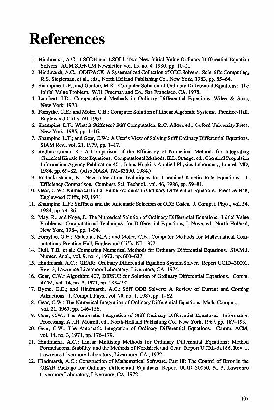
Referen .ces 1. Hindmarsh, A.C.: LSODE and LSODI, Two New Initial Value Ordinary Differential Equation
Solvers. ACM SIGNUM Newsletter, vol. 15, no. 4, 1980, pp. 10-1 1. 2. Hindmarsh, A.C.: ODEPACK A Systematized Collection of ODE Solvers. Scientific Computing,
R.S. Stepleman, et al., eds., North Holland Publishing Co., New Yo&, 1983, pp. 5 5 4 4 . 3. Shampine, L.F.; and Gordon, M.K.: Computer Solution of Ordinary Differential Equations: The
Initial Value Problem. W.H. Freeman and Co., San Francisco, CA, 1975. 4. Lambea J.D.: Computational Methods in Ordinary Differential Equations. Wiley & Sons,
New York, 1973. 5. Forsythe, G.E.; and Moler, C.B.: Computer Solution of Linear Algebraic Systems. Prentice-Hall,
Englewood Cliffs, NJ, 1967. 6. Shampine, L.F.: What is Stiffness? Stiff Computation, R.C. Aiken, ed., Oxford University Press.
New York, 1985, pp. 1-16. 7. Shampine, L.F.; and Gear, C.W.: A User’s View of Solving Stiff Ordinary Differential Equations.
SIAM Rev., vol. 21, 1979, pp. 1-17. 8. Radhakrishnan, K.: A Comparison of the Efficiency of Numerical Methods for Integrating
Chemical Kinetic Rate Equations. Computational Methods, K.L. Strange, ed., Chemical Propulsion Information Agency Publication 401, Johns Hopkins Applied Physics Laboratory, Laurel, MD,
9. Radhakrishnan. K.: New Integration Techniques for Chemical Kinetic Rate Equations. I. Efficiency Comparison. Combust. Sci. Technol., vol. 46,1986, pp. 59-81.
10. Gear, C.W.: Numerical Initial Value Problems in Ordinary Differential Equations. Prentice-Hall, Englewood Cliffs, NJ, 1971.
11. Shampine, L.F.: Stiffness and the Automatic Selection of ODE Codes. J. Comput. Phys., vol. 54, 1984, pp. 74-86.
12. May, R.; and Noye, J.: The Numerical Solution of Ordinary Differential Equations: Initial Value Problems. Computational Techniques for Differential Equations, J. Noye, ed., North-Holland, New York, 1984, pp. 1-94.
13. Forsythe, G.E.; Malcolm, M.A.; and Moler, C.B.: Computer Methods for Mathematical Com- putations, Prentice-Hall, Englewood Cliffs, NJ, 1977.
14. Hull, T.E., et al.: Comparing Numerical Methods for Ordinary Differential Equations. SIAM J. Numer. Anal., vol. 9, no. 4, 1972, pp. 603-637.
15. Hindmarsh, A.C.: GEAR: Ordinary Differential Equation System Solver. Report UCID-3OOO1, Rev. 3, Lawrence Livermore Laboratory, Livermore, CA, 1974.
16. Gear, C.W.: Algorithm 407, DIFSUB for Solution of Ordinary Differential Equations. Comm. ACM, vol. 14, no. 3,1971, pp. 185-190.
17. Byme, G.D.; and Hindmarsh, A.C.: Stiff ODE Solvers: A Review of Current and Coming Attractions. J. Comput. Phys., vol. 70, no. 1, 1987, pp. 1-62.
18. Gear, C.W.: The Numerical Integration of Ordinary Differential Equations. Math. Comput., vol. 21,1967, pp. 146-156.
19. Gear, C.W.: The Automatic Integration of Stiff Ordinary Differential Equations. Information Processing, A.J.H. Morrell, ed., North-Holland Publishing Co., New York, 1969, pp. 187-193.
20. Gear, C.W.: The Automatic Integration of Ordinary Differential Equations. Comm. ACM, vol. 14, no. 3,1971, pp. 176-179.
21. Hindmarsh, A.C.: Linear Multistep Methods for Ordinary Differential Equations: Method Formulations, Stability, and the Methods of Nordsieck and Gear. Report UCRL-51186, Rev. 1, Lawrence Livermore Laboratory, Livermore, CA., 1972.
22. Hindmarsh, A.C.: Construction of Mathematical Software. Part III: The Control of Error in the GEAR Package for Ordinary Differential Equations. Report UCID-30050, Pt. 3, Lawrence Livermore Laboratory, Livermore, CA, 1972.
1984, pp. 69-82. (Also NASA TM-83590, 1984.)
107
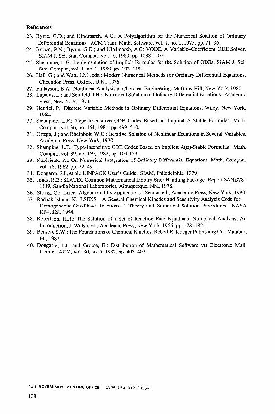
References
23. Byrne, G.D.; and Hindmarsh, A.C.: A Polyalgorithm for the Numencal Solution of Ordinary
24. Brown, P.N.; Byrne, G.D.; and Hindmarsh, A.C: VODE, A Variable-Coefficient ODE Solver.
25. Shampine, L.F.: Implementation of Implicit Formulas for the Solution of OD&. SIAM J. Sci
26. Hall, G.; and Watt, J.M , eds.: Modem Numerical Methods for Ordinary Differential Equations.
27. Finlayson, B.A.: Nonlinear Analysis in Chemical Engineering. McGraw Hill, New York, 1980. 28. Lapidus, L.; and Seinfeld, J.H.: Numerical Solution of Ordinary Differential Equations. Academic
29. Henrici, P.: Discrete Variable Methods in Ordinary Differential Equations. Wiley, New York,
30. Shampine, L.F.: Type-Insensitive ODE Codes Based on Implicit A-Stable Formulas. Math.
31. Ortega, J.; and Rheinbolt, W.C : Iterative Solution of Nonlinear Equations in Several Variables.
32. Shampine, L.F.: Type-Insensitive ODE Codes Based on Implicit A(a)-Stable Formulas Math.
33. Nordsieck, A.: On Numerical Integration of Ordinary Differential Equations. Math. Comput.,
34. Dongarra, J.J , et al.: LINPACK User’s Guide. SIAM, Philadelphia, 1979 35. Jones, R.E.: SLATEC Common Mathematical Library Error Handling Package. Report SAND78-
36. Strang, G.: Linear Algebra and Its Applications. Second ed.. Academic Press, New York, 1980. 37 Radhakrishnan, K.: LSENS-A General Chemical Kinetics and Sensitivity Analysis Code for
NASA
38. Robertson, H.H.: The Solution of a Set of Reaction Rate Equations Numerical Analysis, An
39. Benson, S.W.: The Foundations of Chemical Kinetics. Robert E Krieger Publishing Co.. Malabar,
40. Dongarra, J J.; and Grosse, E.: Distribution of Mathematical Software via Electronic Mail
Differential Equations ACM Trans. Math. Software, vol. 1. no. 1, 1975, pp. 71-96.
SIAM J. Sci. Stat. Comput., vol. 10, 1989, pp. 1038-1051.
Stat. Comput., vol. 1, no. 1, 1980, pp. 103-118.
Clarendon Press, Oxford, U.K., 1976.
Press, New York, 1971
1962.
Comput., vol. 36, no. 154, 1981, pp. 499-510.
Academic Press, New York, 1970
Cornput., vol. 39, no. 159, 1982. pp. 109-123.
vol 16, 1962, pp. 2249.
1189, Sandia National Laboratories, Albuquerque, NM, 1978.
Homogeneous Gas-Phase Reactions. 1 Theory and Numerical Solution Procedures RP-1328. 1994.
Introduction, J. Walsh, ed., Academic Press, New York, 1966, pp. 178-182.
FJ-, 1982.
Comm. ACM, vol. 30, no 5,1987, pp. 403407.
*US G O V E R N M E N T P R I N T I N G OFFICE 1 9 9 5 - t 5 0 - 0 1 2 - 0 3 5 5 4
108

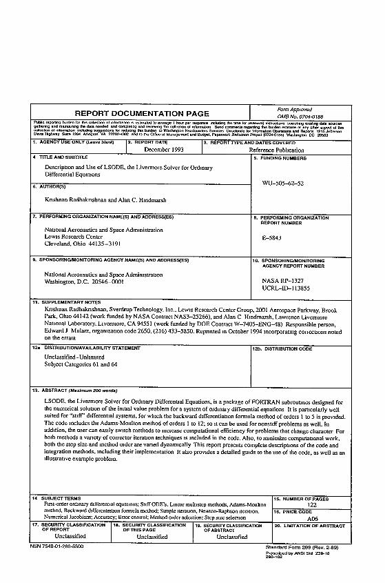
REPORT DOCUMENTATION PAGE I ~
1. AGENCY USE ONLY (Leave 12 REPORT DATE 13. REPORTTYPE AND DATES COVERED
December 1993 4 TITLE AND SUBTKLE
Descripuon and Use of LSODE, the Livermore Solver for Ordinary Differential Equauons
6. AUTHOR(S)
Knshnan Radhaknshnan and Alan C. Hindmarsh
7. PERFORMING ORGANIZATION NAME(S) AND ADDREWES)
Nauonal Aeronautics and Space Admnistration Lewis Research Center Cleveland, Ohio 44135-3191
9. SPONSORINWUONKORING AGENCY NAME(S) AND ADDREWES)
National Aeronautics and Space Administrauon Washington. D.C. 20546-0001
11. SUPPLEMENTARY NOTES
:ference Publication 5. FUNDING NUMBERS
\VU-505-62-52
B. PERFORMING ORGANIZATION REPORT NUMBER
E-5843
0. SPDNSORlNWUONlTORlNG AGENCY REPORT NUMBER
NASA RP-1327 UCRL-ID-I 13855
Knshnan Radhaknshnan, SverdrupTechnology, Inc.. Lewis Research Center Group. 2001 Aerospace Parkway. Brook Park, Ohio 44142 (work funded by NASA Contract NAS3-25266). and Alan C Hindmarsh. Lawrence Livermore Nauonal Laboratory. Livermore. CA 94551 (work funded by DOE Contract \V-7405-ENG48) Responsible person, Edward J Mularz, organizauon code 2650, (216) 433-5850. Repnnted in October 1994 incorporaung correcuons noted on the errata
12a DISTRIBUllONIAVAILABI!JTY STATEMENT I1Zb. DISTRIBUllON CODE
Unclassified - Unlimted Subject Categories 61 and 64
LSODE, the Livermore Solver for Ordinary Differential Equations, is a package of FORTRAN subrouunes designed for the numerical soluuon of the iniual value problem for a system of ordinary differential equations It is particularly well suited for "suff differential systems. for which the backward differeniiauon formula method of orders 1 to 5 is provided. The code includes the Adams-Moulton method of orders 1 to 12; so it can be used for nonsuff problems as well. In addition. the user can easily switch methods to increase computational efficiency for problems that change character For both methods a vanety of corrector iterauon techniques is included in the code. Also. to minimize computauonal work. both the step size and method order are vaned dynmcally This report presents complete descripuons of the code and integration methods, including their implementation It also provides a detailed guide to the use of the code, as well as an illusuauve example problem.
14 SUBJECTTERMS 15. NUMBEROFPAGES Fim-order ordinary dilTerentlal quaiions: Stiff ODE'S. Lincar multistep mahods. Adam-Moulion 122
A06 mehod, Backward diffemniiauon formula method: Smplc iterauon. Newton-Raphson nerauon. Numerical Jacobians: Accuracy; Error convot Muhod order selection: Step size selection
16. PRICE CODE
17. SECURITY CLASSIFICATION 18. SECURrPl CLASSIFICATION 19. SECURrrY CUSSIFICATION 20. LIMKATION OF ABSTRACT OF REPORT OFTHIS PAGE OF ABSTRACT
Unclassified Unclassified Unclassified ISN 7540-01-280-5500 Standard Farm 298 (Rev. 2-89)
Prewrbed by ANSI Sld 234.18 288102


National Aeronautics and Space Administration Lewis Research Center 21000 Brookpark Rd. Cleveland, OH 441 35-31 91
Officlal Business Penalty for Private Use $300
POSTMASTER: If Undeliverable - Do Not Return
Related Documents


