Description and Evaluation of GDEM-V 3gcoos.tamu.edu/products/data/ts_profile/GDEMV-3.pdf · Description and Evaluation of GDEM-V 3.0 ... information if it does not display a currently

Naval Research LaboratoryStennis Space Center, MS 39529-5004

NRL/MR/7330--09-9165

Approved for public release; distribution is unlimited.

Description and Evaluation of GDEM-V 3.0MICHAEL R. CARNES

Ocean Sciences Branch Oceanography Division

February 6, 2009

i

REPORT DOCUMENTATION PAGE Form ApprovedOMB No. 0704-0188

3. DATES COVERED (From - To)

Standard Form 298 (Rev. 8-98)Prescribed by ANSI Std. Z39.18

Public reporting burden for this collection of information is estimated to average 1 hour per response, including the time for reviewing instructions, searching existing data sources, gathering and maintaining the data needed, and completing and reviewing this collection of information. Send comments regarding this burden estimate or any other aspect of this collection of information, including suggestions for reducing this burden to Department of Defense, Washington Headquarters Services, Directorate for Information Operations and Reports (0704-0188), 1215 Jefferson Davis Highway, Suite 1204, Arlington, VA 22202-4302. Respondents should be aware that notwithstanding any other provision of law, no person shall be subject to any penalty for failing to comply with a collection of information if it does not display a currently valid OMB control number. PLEASE DO NOT RETURN YOUR FORM TO THE ABOVE ADDRESS.

5a. CONTRACT NUMBER

5b. GRANT NUMBER

5c. PROGRAM ELEMENT NUMBER

5d. PROJECT NUMBER

5e. TASK NUMBER

5f. WORK UNIT NUMBER

2. REPORT TYPE1. REPORT DATE (DD-MM-YYYY)

4. TITLE AND SUBTITLE

6. AUTHOR(S)

8. PERFORMING ORGANIZATION REPORT NUMBER

7. PERFORMING ORGANIZATION NAME(S) AND ADDRESS(ES)

10. SPONSOR / MONITOR’S ACRONYM(S)9. SPONSORING / MONITORING AGENCY NAME(S) AND ADDRESS(ES)

11. SPONSOR / MONITOR’S REPORT NUMBER(S)

12. DISTRIBUTION / AVAILABILITY STATEMENT

13. SUPPLEMENTARY NOTES

14. ABSTRACT

15. SUBJECT TERMS

16. SECURITY CLASSIFICATION OF:

a. REPORT

19a. NAME OF RESPONSIBLE PERSON

19b. TELEPHONE NUMBER (include areacode)

b. ABSTRACT c. THIS PAGE

18. NUMBEROF PAGES

17. LIMITATIONOF ABSTRACT

Description and Evaluation of GDEM-V 3.0

Michael R. Carnes

Naval Research LaboratoryOceanography DivisionStennis Space Center, MS 39529-5004 NRL/MR/7330--09-9165

Approved for public release; distribution is unlimited.

UL 24

Michael R. Carnes

(228) 688-5648

The GDEM (Generalized Digital Environment Model) has served as the U.S. Navy’s global gridded ocean temperature and salinity climatology since its development began in 1975. This memorandum introduces a new version of this climatology, named GDEM-V 3.0, and discusses the techniques used in its construction. Several comparisons are shown between version 3.0 and the previous version (2.6) of GDEM to demonstrate

function and replace it by a method that horizontally interpolates temperature or salinity values separately at each depth level. In addition, the

06-02-2009 Memorandum Report

One Liberty Center875 North Randolph St.Arlington, VA 22203-1995

73-6728-08-5

ONR

0602435N

CONTENTS

iii

1. Introduction ...............................................................................................................................................1

.........................................................................................................................................2

......................................................................................................................................................3

......................................................................................................5

.................................................................................................6 ..............................................................................................................................8

........................................................................................................11 .......................................................................................................14

.............................................................................................................................14....................................................................................................................19

..............................................................................................................................................19

............................................................................................................................................20

1. Introduction An ocean climatology of temperature and salinity provides a convenient condensation of information obtained from the large collection of profiles measured over a long period of time. The best known and most-used global ocean climatologies include several revisions of NOAA’s World Ocean Atlas (WOA) (Levitus, 1982; Levitus et al., 1994), the Hydrobase climatology (Lozier et al., 1994a; MacDonald et al., 2001), and the World Ocean Circulation Experiment (WOCE) climatology. . Each of these have limitations which make them unuseable for many Navy applications. NOAA’s climatology uses long length scales (700 km) and a 1 resolution horizontal grid, making it inappropriate for coastal regions and inland seas. The Hydrobase and WOCE climatologies only use profiles containing both temperature and salinity (excluding most expendable profiles, such as XBTs), and both climatologies are constructed only where bottom depth is greater than 200 m. The GDEM (Generalized Digital Environmental Model) was developed to provide a climatology tailored to the Navy’s needs and to enable use of classified profiles available only to the navy. Development of GDEM at the Naval Oceanographic Office began in 1975 and culminated in the first release to the Navy community in 1984. The first release contained only the North Atlantic region, but by 1991 most of the world’s oceans were included. The techniques employed to construct GDEM are documented in Teague et al. (1990). This early version of GDEM is a four-dimensional (latitude, longitude, depth, and time) digital model of temperature and salinity, where the vertical profiles are generated from the stored coefficients of mathematical functions. The horizontal grid resolution is ½ in latitude and longitude and the temporal resolution is one month. The particular functional forms used to represent the vertical profiles restricted the database to regions where bottom depth is 100 m deep or greater. Later, this minimum depth requirement was relaxed to 50 m. Another version of GDEM called Master GDEM 5 was introduced in 1994 that included horizontal grids computed at higher resolutions, up to 1/6 , for several regions such as the Gulf of Aden, the Persian Gulf, the Yellow Sea and the East China Sea, and the Arabian Sea. In 1994, the name was changed to GDEM-V, where the V was added to indicate that horizontal resolution grid resolution was variable. This version also included gridded climatologies of the Yellow Sea and the Persian Gulf computed by a new technique which allows results to be produced at locations where bottom depths are as shallow as 5 m. The version is currently available from the Navy’s Oceanographic and Atmospheric Master Library (OAML) is named GDEM-V 2.6 (henceforth called GDEM2). Several problems in the GDEM2 have been identified. Most result from the methods used in its construction. Some limit its applicability and others result in obviously erroneous temperature and salinity structure in some regions of the world’s oceans. Previous upgrades to GDEM made small additions or revisions. However, to remove the identified problems, a completely new version of GDEM has been developed and named GDEM-V 3.0 (henceforth called GDEM3) using techniques not previously used to construct GDEM. This upgrade replaces the previous global monthly climatologies of

1

_______________

Manuscript approved December 30, 2008.

temperature, salinity, and temperature standard deviation, and adds the climatology of salinity standard deviation. The purpose of this document is to describe the new climatology and the techniques used in its construction, and to compare GDEM3 with the previous version. Several examples are given to demonstrate the improved performance of version 3 over version 2.6. Primarily because of the issues discussed in the next section concerning the profile data set being used, we consider GDEM3 to be a temporary climatology that will be replaced once a newly edited data set becomes available. 2. Profile Data Set The GDEM3 was computed from temperature and salinity profiles extracted from the Master Oceanographic Observational Data Set (MOODS) in 1995. The profiles were edited by personnel at the Naval Research Laboratory (NRL) and then used to construct the climatology of the Modular Ocean Data Assimilation System (MODAS) (Fox et al., 2001, 2002). NRL manually examined all profiles within groups covering small geographical regions and small seasonal or monthly time periods in order to identify and remove anomalous profiles. This data set contains only about 2.7 million profiles, whereas MOODS will soon contains over 8 million edited profiles. The number of profiles in the MODAS data set (used to construct GDEM3) and the number of profiles (soon available) in MOODS are shown in Figures 1a and 1b, respectively. Each plot displays bar charts of the number of profiles measured each year from 1900 to the present. The black bars indicate the number of profiles that contain temperature, but not salinity, and the red bars, stacked on top of the black bars, indicate the number of profiles that have both temperature and salinity.

Each profile was interpolated, using the method of weighted parabolas (Reiniger and Ross, 1968), to a set of 78 standard depths ranging from the surface to 6600 m. The NOAA WOA contains only 33 level down to 5500 m and GDEM2 contains 35 levels down to 5500 m. The larger number of standard depths used in GDEM3 results in a larger final climatology, but has two main advantages. First, the deepest standard depth above the bottom at any location is generally closer to the bottom. Acoustic applications of GDEM often require that each profile be extrapolated to the bottom depth. This procedure is more accurate when the starting point is closer to the bottom. Secondly, the technique used here simultaneously minimizes the error of the gridded profiles to both the observed values and the vertical gradients of the observed profiles. Better estimates of the vertical gradients are obtained using the higher-resolution vertical grid. The very sparse set of Arctic Ocean profiles in the MODAS and GDEM3 data set was supplemented by temperature and salinity profiles extracted from the gridded PHC (Polar science center Hydrographic Climatology) (Steele et al., 2001). The PHC was constructed by merging the global WOA98 (Antonov, et al., 1998; Boyer et al., 1998) with the regional Arctic Ocean Atlas (EWG, 1997; 1998).

2

Figure 1. The number of profiles each year from 1900 to 2000 in (a) the profile database used to construct the MODAS and GDEM-V 3.0 climatologies, and (b) the number of profiles in MOODS.

3. Method The new GDEM construction software produces global 3-dimensional monthly grids of temperature, salinity, temperature standard deviation, and salinity standard deviation. The horizontal grid resolution is 1/4 and the vertical grid has 78 depths from the surface to 6600 m. The horizontal grid spacing of GDEM2 is primarily1/2 degree and the vertical grid contains 35 depths down to 5500 m. GDEM2 uses a higher-resolution horizontal grid only in the selected regions such as the Yellow Sea, the Persian Gulf, and the Baltic Sea. The GDEM3 climatology for each month of the year was produced by first gridding the observations on each depth surface over the entire domain. A second step then adjusted the vertical structure of the gridded result to better match the vertical gradient of the observations. A final step adjusts the vertical structure of both temperature and salinity to ensure that each profile is statically stable. The horizontal gridding of profile values or coefficients in previous versions of GDEM was performed using the minimum curvature method (Briggs, 1974; Swain, 1976). Smith et al. (1990) later showed that this technique might produce large erroneous oscillations, particular in data-sparse regions of the interpolated grid. They also showed that adding a tension term to the interpolation equations could eliminate such oscillations. The minimum curvature technique was shown by Panteleev et al. (1989, 1995) to be preferable to optimal interpolation (used in the gridding of the MODAS climatology) unless the covariance length scales of the data being gridded are known accurately. The interpolation equations for a discrete grid are derived by simultaneously minimizing, with respect to each gridded value, the squared difference between the observations and the gridded values (minimizing the data error) plus the squared second derivative of the gridded quantity (minimizing the curvature), with respect to the coordinate values. The tension term is added by also minimizing the squared first derivative of the gridded values (minimizing the slopes). This technique was used by Brasseur et al.(1996) to grid

3

temperature and salinity on a finite element grid to produce the Mediterranean Oceanic DataBase (MODB). Experiments leading to the development of GDEM3 determined that the most robust approach was obtained by retaining the slope minimization term and eliminating the curvature minimization term. Use of the curvature term results in unrealistic gridded values and gradients in data-sparse regions, particularly near shore, even with the constraint provided by the slope (tension) term. Therefore, the GDEM3 interpolation equations were derived by minimizing only the data error and the squared slope. Also, zero-gradient boundary conditions were applied along land boundaries at each depth to eliminate gridding over land and across land boundaries. The minimum curvature technique applied to previous versions of GDEM did not eliminate gridding over land, and resulted in mixing unlike water types separated by narrow land boundaries. The optimum interpolation gridding approach used to generate the NOAA and MODAS climatologies attempts to produce the same result by grouping profiles withn regional polygons on each side of land boundaries, and interpolating the profiles only within each polygon. This is a tedious approach that must be reformulated at each depth, and the correct approach to use near narrow straits is unclear. The gridding of the temperature, salinity, temperature variance, and salinity variance was performed separately at each of the 78 depth levels. The preferred approach is to perform the gridding on potential density surfaces as was done for the Hydrobase and WOCE climatologies as recommended in Lozier et al. (1994b). Averaging on constant depth or pressure surfaces in areas of sharply sloping isopycnals can produce water masses with profiles of potential temperature-versus-salinity which are uncharacteristic of the local water masses. Gridding on isopycnal surfaces requires that both temperature and salinity be present on each observed profile (because potential density is needed), eliminating the use all XBT profiles. Also, in the vertically-mixed layer near the surface or in well-mixed coastal waters where the surface of constant density is nearly vertical, this approach is difficult or impractical to apply. For this reason, the Hydrobase and WOCE climatologies do not grid data in shallow water. The distribution of observations can change significantly between consecutive depth levels (or between density levels) due to differences in the maximum depth of the available profiles. The local mean computed at each depth from this changing distribution can therefore contain unrealistic vertical gradients. This situation results from combining profiles measured by different instruments (XBTs profiles ending near 200m, 400m, or 800 m, and CTD profiles ending near the bottom) or when maximum profile depths are limited to the variable local bottom topography. No climatology other than the previous version of GDEM made any attempt to compensate for this changing data distribution versus depth. The GDEM2 approach fits each profile to an analytical function defined over a pre-set depth range, implicitly extending each profile to that depth range. However, the function-fitting approach leads to several other problems, and was therefore not used in the construction of GDEM3. Instead, the vertical gradient of each vertical profile in the final gridded climatology was corrected by an objective least-squares technique which forces the vertical gradient of each gridded profile toward the gradient estimated from the data while simultaneously minimizing the difference between

4

the original and modified gridded profile. This approach is very effective at eliminating the large erroneous near-bottom vertical gradients often evident in climatologies.

The observations were gridded by a slightly different technique in each of three different, but overlapping, depth ranges. Once computed, the grids in the three depth domains were smoothly spliced together to form the final single grid for each variable and for each month. In the deepest layer, extending from 1000 m to the bottom, the seasonal variability and the number of observations are both low. The annual average was computed in this layer by gridding all profiles, independent of their month of observation. In the middle layer, between 200 m and 1000 m, seasonal changes are typically small but significant in some regions. There are too few observations in many areas within a single month or season, particularly for salinity, to adequately resolve the dominant temperature and salinity structure. To compensate, the analysis for the mid-depth domain was performed for each month using three months of observations centered on the analysis month. Also, instead of gridding the profile values, the difference between the observations and the annual mean were first computed and gridded. Once computed, the gridded anomalies were added back to the annual mean. In the upper layer between the surface and 200 m where observation density and seasonal variability are highest, the grid for each month was computed from the three months of observations centered on the analysis month. The vertical gradient correction was applied to the gridded mean profile at each grid location and for each of the three methods (one for each depth range) before being spliced together to form the final full-depth profiles. The final step in the preparation of the monthly gridded climatologies was the adjustment of the temperature and salinity profile at each grid location to produce a statically stable profile. Due to the vertical gradient correction already applied, the number and severity of instabilities were small. Unstable segments on each profile were identified by the negative squared Brunt-Vaisala frequency (Jackett et al., 1995) computed from the temperature and salinity. Once identified, the local temperature and salinity were modified iteratively until a stable profile was produced. 4. Comparison of GDEM3 and GDEM2 GDEM is being upgraded from version 2 to 3 to remove significant errors and deficiencies found in GDEM2. GDEM2 has served the Navy well for many years, but it has a number of problems, listed below: 1. Gridding performed by minimum curvature interpolation without tension. Grids

through land. 2. Temperature and salinity are not gridded in shallow water except in a few small

regions. 3. Important coastal fronts are not resolved because of grid resolution and the methods

used. 4. The curve-fitting approach used to represent vertical profiles has always been

controversial and sometimes fails. 5. The vertical structure is unstable at many locations. This is also a common problem

with NOAA’s WOA.

5

6. The database was stored using only two decimal places for temperature and salinity. Three decimal places are required to adequately resolve the deep salinity structure.

7. The vertical grid resolution is too low. 8. The historical profile data base has increased significantly since the most recent

update. 9. The present GDEM2 database does not include standard deviation of salinity. This section shows examples of some of these problems by comparing the results from GDEM2 with GDEM3. In some cases, comparisons are also made to the NOAA World Ocean Altas. These examples comprise only a small subset of the problems encountered in GDEM2 and the improvements obtained in GDEM3. 4.1 Gridding around land boundaries The minimum-slope gridding algorithm used with GDEM3 masks out all land positions at each depth and employs zero-gradient boundary conditions along the land boundaries. As a result, interpolation of temperature or salinity on one side of a land boundary has no effect on the gridded value on the other side of the boundary. However, if a nearby sea passage through the land boundary exists, then the observations on one side may have a small influence on the other side. The GDEM2 minimum curvature algorithm contains no land masking so that observations can influence gridded values across a land boundary. The errors produced due to the lack of land masking are shown in the plot of GDEM2 temperature at 1000-m depth in and around the Sulu Sea between the Philippines and Borneo in Figure 2a. Comparison of the two plots reveals that the isolated higher temperatures (about 10 C) at this depth in the Sulu Sea have been erroneously blended by the GDEM2 gridding algorithm with the lower-temperature water (about 4 C to 4.5 C) of the surrounding seas. The separate identity of the various water masses is maintained in GDEM3 (Figure 2b). Plots of temperature at 4000 m in the region ranging from India to Australia (Figure 3) reveal several other regions where errors in the GDEM2 temperature have been produced by the non-land-masked minimum-curvature gridding algorithm. An enlarged view of the GDEM2 plot is shown in Figure 4. Temperature rises 0.5 C northward toward the edge of land south of the Bay of Bengal in the GDEM2 plot. This error (very large compared to the true temperature variability at this deep level) probably results from a northward extrapolation into the data-sparse region next to the bottom at 4000 m depth. The minimum curvature technique tends to extrapolate the horizontal gradient provided by the closest observations. Extrapolations by the GDEM3 minimum-slope gridding algorithm tend to flatten out and maintain the value of the closest observations. Similar looking errors in GDEM2 are found east of the Philippines, south of Java, and along the equator north of Papua New Guinea. These cases appear to be the result of blending with higher-temperature water (across land barriers) of the small interior seas.

6

Figure 2. Temperature in and surrounding the Sulu Sea from (a) GDEM-V 2.6 and (b) GDEM-V 3.0.

Figure 3. Temperature at 1000 m around the East Indian Archipelago from (a) GDEM-V 2.6 and (b) GDEM-V 3.0.

7

Figure 4. Enlarged view of the temperature at 4000 m from GDEM-V 2.6.

4.2 Vertical profile GDEM2 fits a non-linear function of 6 coefficients to profiles in the upper 400 m and then grids the coefficients of those profiles. This curve-fitting approach fails with some types of profiles, caused either by an inappropriate application of the technique or to the inability of the prescribed function to fit the profiles. Although many examples of poor vertical profile fitting are found in the GDEM2 database, the technique performs adequately in most regions, and despite its drawbacks, the GDEM2 function fitting technique is nearly unique in its attempt to provide a vertically coherent gridding algorithm. The GDEM2 gridding approach sometimes fails for various reasons. This first example is taken from the tropical north central Pacific and is displayed on a screen shot from the ODDESA editor, which is being used to edit the eight million profiles in MOODS. The left frame shows the location, with the small black dots indicating the position of observed profiles and the larger magenta dot showing the position of the climatology profiles. The right frame shows a composite plot of all observed salinity profiles as thin black lines, and the salinity profiles from the GDEM2, GDEM3, and WOA climatologies as thick colored lines. The data sets used in each of the climatologies are slightly different, and might contribute to the differences. The GDEM2 upper-400 m fit underestimates the sharp maximum at 100 m, but is otherwise good. The problem apparently occurred when the 0-to-400 m fit was spliced to the mid-depth profile functional fit. The method used removes one or more salinity values around 400 m from each of the fitted profiles, and then estimates salinity in the remaining gap using a cubic

8

spline. The cubic spline overshoots the salinity minimum due to the sharp gradient between 100 m and 200 m. Both GDEM3 and WOA fit the profiles well. However, the WOA profile is noisy because salinity was gridded (horizontally) separately at each depth, whereas the GDEM3 profile is smooth because an additional step is performed to correct the vertical gradient.

Figure 5. Screen shot from the ODDESA profile editor showing observed (black dots and black lines) and climatological (thick colored lines) salinity in the tropical north central Pacific Ocean. The GDEMV-2.6 profile overshoots the minimum due to the method for splicing upper (0 to 400 m) and mid-depth profiles together.

The next example is from February in the Black Sea. It shows GDEM2 at its worst, and is not representative of the climatology throughout the rest of the world. Figures 6a and 6b are plots of temperature at a depth of 100 m in February from GDEM3 and GDEM2, respectively. The contour interval in both plots is 0.1 C and the colors representing the temperature ranges is the same for both plots. The simple thermal structure with two cyclonic gyres shown in the GDEM3 plot (Figure 6a) is the expected result, based on many previous studies (e.g., page 183 of Neumann and Pierson, 1966). The plot from GDEM2 (Figure 6b) exhibits a much larger range of temperature and a chaotic small-scale variability. The cause of the strange temperature map in the GDEM2 plot is explored in the next figure. Figure 7 shows an ODDESA editor screen dump of temperature profiles from the vicinity of the anomalously low-temperature patch centered near the position 37 E and 43.5 N in Figure 6b. The black dots in the left frame are the positions of all temperature observations found the MODAS/GDEM3 data set during the three-month period from January through March. The square red box delineates a subset region, and the magenta dot at its center is the position of the GDEM2, GDEM3, and WOA climatological profiles displayed in the right frame. The observed temperature

9

profiles within the subset region are plotted as thin black lines in the right frame. The observed profiles exhibit an unusual sharp inverted thermocline (minimum temperature

Figure 6. Temperature (Degrees C) at 100 m depth in the Black Sea in February from (a) GDEM-V 3.0 and from (b) GDEM-V 2.6. The contour interval for both plots is 0.1 C and the colors representing the temperature ranges are the same for each plot.

Figure 7. Screen shot from ODDESA editor showing profiles from January, February, and March from the GDEM-V 3.0 profile database. Red box in left frame delineates subset of profiles shown in right frame.

10

near the top, but stabilized by low surface salinity) due to winter cooling. The GDEM3 and WOA 98 profiles fit the data well (although the WOA profile is noisy), but the GDEM2 algorithm which fits a function to vertical profiles in the upper 400 m is apparently unable to provide an adequate fit. Even in summer conditions, when the normal thermocline structure with maximum temperature at the top prevails, the upper 400 m functional fit by GDEM2 is unable to adequately define the sharp changes in sound speed in the near-surface sound channel as shown in Figure 8.

Figure 8. Screen dump from ODDESA profile editor displaying all profiles positions in the left frame containing both temperature and salinity in July, August, and September. The right frame shows profiles of sound speed computed from profiles within the red box in the left frame. 4.3 Vertical gradient correction This vertical gradient correction employed by GDEM3 is designed to reduce the bias in the mean profiles created by gridding sets of profiles with different lengths. In deep water, a diverse set of profiles are found, including 200-m, 400-m, and 800-m XBTs, and longer profiles from CTDs and bottle data. In shallow water, profile depths can vary locally due to rapid changes in bottom topography. Figure 9 shows a group of temperature profiles from March over a small region in the Yellow Sea. A simple temperature average at each depth will result in a bias toward lower temperatures at the surface and higher temperatures at the greater depths, perhaps resulting in an unstable profile.

11

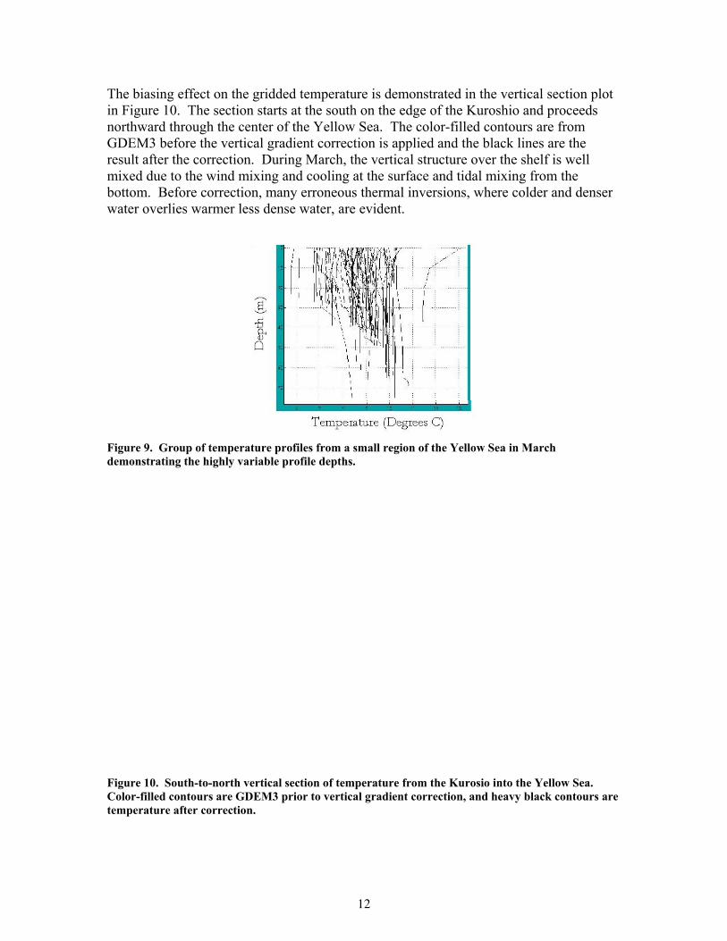
The biasing effect on the gridded temperature is demonstrated in the vertical section plot in Figure 10. The section starts at the south on the edge of the Kuroshio and proceeds northward through the center of the Yellow Sea. The color-filled contours are from GDEM3 before the vertical gradient correction is applied and the black lines are the result after the correction. During March, the vertical structure over the shelf is well mixed due to the wind mixing and cooling at the surface and tidal mixing from the bottom. Before correction, many erroneous thermal inversions, where colder and denser water overlies warmer less dense water, are evident.

Figure 9. Group of temperature profiles from a small region of the Yellow Sea in March demonstrating the highly variable profile depths.

Figure 10. South-to-north vertical section of temperature from the Kurosio into the Yellow Sea. Color-filled contours are GDEM3 prior to vertical gradient correction, and heavy black contours are temperature after correction.

12

The next example, Figure 11, shows a vertical section of temperature from the WOA at nearly the same position as Figure 10. The WOA 98 contours (color filled) exhibit a large temperature inversion between 100 m and 150 m. At the edge of the shelf, the temperature above 100 is biased toward the lower shelf temperatures, but the bias disappears at depths deeper than the Yellow Sea shelf. The bias is exaggerated in WOA due to its use of long length scales in its gridding algorithm. The inversions are absent in the corrected GDEM3 temperature contours (heavy black lines in Figure 11).

Figure 11. South-to-north vertical section of temperature from the Kurosio into the Yellow Sea. Color-filled contours are from WOA 98, and the heavy black contours are from GDEM3.

The technique for correcting the vertical gradient is objective and robust, but quadruples the calculation time. The temperature gradient correction requires prior calculation of 3-D grids of temperature, temperature standard deviation, temperature difference between consecutive levels, and the standard deviation of the temperature difference (similarly for salinity). Then at each horizontal grid location, a new temperature vertical profile is computed by minimizing the following sum with respect to each value of the final temperature profile . T̂

2 2

1

1 2

ˆ ˆ ˆN Nk k k k k

k kk k

T T T T DE A

N

k

where, gridded temperature profile at depth levels 1,

gridded temperature standard deviation

gridded temperature difference (depth level level 1)

gridded temperature difference standard devia

k

k

k

k

T k

D k

tion.

13

The first term tries to keep the new profile as close to the original profile as possible, and the second term tries to keep the vertical gradient of the final solution close the gridded vertical gradient. Solution of the minimization of this equation (using zero second-derivative boundary conditions) results in a tri-diagonal system of equations which is solved for the new temperature profile, , at each horizontal grid location. T̂ 4.4 Shallow continental shelves Early versions of GDEM gridded temperature and salinity only up to the 100-m isobath, eliminating the climatology over most of the continental shelves. Later, it was extended to the 50 m isobath, although a few regions such as the Yellow Sea, Persian Gulf and Baltic were computed by a different technique and were gridded up to about the 5 m bottom contour. Unfortunately, the upgrade from the 100-m to the 50-m isobath was apparently not implemented correctly, and shallow shelf profiles were not used. The result of this omission is clearly demonstrated in Figure 12a which shows the GDEM2 surface salinity in the Gulf of Mexico in January. GDEM2 shows no hint of the low shelf salinity which originates from the fresh water influx from rivers, whereas it is clearly evident in the GDEM3 plot (Figure 12b). The contour interval on both plots is 0.5 psu.

Figure 12. Surface salinity for January in the Gulf of Mexico from (a) GDEM-V 2.6 and (b) GDEM-V 3.0. The contour interval on plot plots is 0.5 psu. A similar result is found in the Gulf of Tonkin where outflow from the Red and Black rivers should produce a lower salinity near the coast. The GDEM2 plot (Figure 13a) shows one small pocket of low salinity, while GDEM3 clearly displays the low coastal salinities. Although GDEM3 does show the low salinity, the gridding in climatologies tends to smooth the coastal salinities too far out to sea, particularly if the density of observations is low and the length scales of the gridding is large. 4.5 Coastal fronts The next series of plots demonstrates the improved representation of coastal fronts in GDEM3 as compared to those in GDEM2 and in WOA. The first (Figure 13) compares the GDEM3 and GDEM2 July salinity at 200 m depth in the vicinity of the Yucatan Current, the Loop Current, and the Florida Current. The Loop Currents is poorly defined

14

by GDEM2 and the other two fronts are nearly non-existent. All fronts in this region arewell defined by GDEM3. Some of the differences between the two can be attributed to the lower grid resolution of GDEM2 (1/2 degree) as compared to GDEM3 (1/4 degree), but much of the improvement in GDEM3 is likely due to the land masking in the gridding algorithm. Masking helps to mainta

in coastal gradients by eliminating interpolation (and oothing) across land boundaries.

sm

Figure 13. Salinity at 200 m depth in July from (a) GDEM-V 3.0 and (b) GDEM-V 2.6.

. The low 1 solution of WOA is inadequate for representation of these fronts.

The same comparison is made to the WOA climatology in Figure 14re

Figure 14. Salinity at 200 m depth in July from (a) GDEM-V 3.0 and (b) WOA 98.

15

Variability of the Florida Current position is low as it moves along the edge of the BlakePlateau. Therefore, a climatological representation of the front, using all available profiles, should have horizontal gradients nearly as high as that from a synoptic view of the front if the horizontal grid resolution is high enough. Figures 15a and b show west-to-east vertical sections through the Florida Current at 29.5 N (north of Daytona BeachFlorida), contoured from the GDEM3 and GDEM2 climatologies, respectively. Neasynoptic vertical sections indicate that the 14 C isotherm should intersect the slope at about 200 m depth, whereas in this occurs at about 280 m in GDEM3 and 420 m in GDEM2. Experiments w

, rby

ith grid resolution in GDEM3 determined that isotherms slopes can be increased to those found in synoptic sections across the Florida Strait using a 1/8 horizontal grid interval.

Figure 15. Vertical section of temperature across the Florida Current at 29.5 N in May,eastward from Florida from (a) GDEM-V 3.0 and (b) from GDEM-V 2.6.

Figure 16 shows the same section for both GDEM3 (again) and the WOA 98

drawn

climatology. The Florida Current is essentially missing in WOA 98 because the grid resolution (one degree of latitude and longitude) is wider than the width of the front.

Figure 16. Vertical sectino of temperature across the Florida Current at 29.5 N in May, draweastward from Florida from (a) GDEM-V 3.0 and (b) WOA 98.

n

16

Figure 17 shows plots of the temperature at 400 m in the Florida Current and Gulf Stream made from the GDEM3 and GDEM2 climatologies. After leaving the coast Cape Hatteras, the Gulf Stream frontal structure is resolved well by GDEM2, but the peak gradients shown by GDEM3 are higher. However, the isotherm positions are noisier in GDEM3 due to the variability of the front and to the Gulf Stream rings samplealong its sides. In the design of climatologies, there is a tradeoff between resolution asmoothness. A climatology is usually meant to represent the true long-term average of the temperature and salinity fields. Undersampling of transient features like rings or frontal meanders results in a noisy estimated climatology. The noise can be suppresseby increasing the l

at

d nd

d ength scales or other smoothness parameters used in the interpolation,

but then any ocean features sampled adequately (such as the Florida Current) will be overly smoothed.

Figure 17. Temperature at 400 m depth in March from (a) GDEM-V 3.0 and (b) GDEM-V 2.6.

An extreme case of over smoothing in the near-coastal domain (the same region as Figure 17) is shown by WOA 98 in Figure 18b. In this example, the Slope Water, inshore of the Gulf Stream, has disappeared and replaced by the Gulf Stream front.

17

Figure 18. Temperature at 400 m depth in March from (a) GDEM-V 3.0 and (b) WOA 98.

Many other examples of inadequate resolution of coastal fronts are found in GDEM2. Figure 19 shows sound speed in June at 200 m along the Kurosio, from where its flow begins northward of the Philippines and then along the coast of Taiwan and into the Ryuku Trough inside the Sensei Islands. The color-filled contours are from GDEM3 and the Black lines are from GDEM2. GDEM2 misses much of this shallow front.

Figure 19. Sound speed at 200 m in June from GDEM3 (color-filled contours) and GDEM2 (heavy black lines).

18

4.6 Precision truncation Temperature and salinity values are truncated in GDEM2 to 2 decimal places (0.01 precision) to reduce the size of the data base. The resulting precision is adequate for sound speed computed from temperature and salinity, but is too coarse to resolve the salinity structure of the deep ocean. Figure 20 illustrates the problem with a vertical section of salinity from the Equator to 60 N along 166 E within the depth range from 2000 m and 5000 m. The GDEM2 contours (color-filled) and the GDEM3 contours (heavy black lines) are both drawn using a contour interval of 0.01 (the same as the GDEM2 precision). Because both the precision and the contour interval is set to 0.01, the GDEM2 contours jump rapidly between standard depth levels (at 500 m intervals below 2000 m), and do a poor job of defining the deep salinity structure. The GDEM3 database is also compressed (to 16 bit integers) by use of an offset and scale factor, but with little apparent effect on the result.

Figure 20. Vertical section of salinity below 2000 m depth from the Equator to 60 N along 166 E. The contour interval for both GDEM2 (color-filled contours) and GDEM3 (heavy black contours) is 0.01. 5. Conclusion GDEM3 has been accepted in OAML as a replacement for GDEM2. The methods used to construct GDEM3 are totally different than those used with GDEM2. Comparison of these two climatologies in the above examples demonstrates several significant improvements by GDEM3.

19

REFERENCES Antonov, J.I., S. Levitus, T.P. Boyer, M.E. Conkright, T.D. O’Brien, and C. Stephens, 1998, World Atlas 1998 Vol. 1: Temperature of the Atlantic Ocean, NOAA Atlas NESDIS 27, U.S Government Printing Office, Washington, D.C. Boyer, T.P., S. Levitus, J.I. Antonov, M.E. Conkright, T.D. O’Brien, and C. Stephens, 1998: World Ocean Atlas 1998 Vol. 4: Salinity of the Atlantic Ocean, NOAA Atlas NESDIS 20, U.S. Government Printing Office, Washington D.C. Brasseur, P., J.M. Beckers, J.J. Brankart, and R. Schoenauen, Seasonal temperature and salinity fields in the Mediterranean Sea: Climatological analyses of an historical data set. Deep-Sea Res., 43, 159-192, 1996. Briggs, I.C., Machine contouring using minimum curvature, Geophysics, 30, 39-48, 1974. Environmental Working Group (EWG), 1997: Joint U.S.-Russian Atlas of the Arctic Ocean for the Winter Period [CD-ROM], Natl. Snow and Ice Data Cent., Boulder, Colorado. Environmental Working Group (EWG), 1998: Joint U.S.-Russian Atlas of the Arctic Ocean for the Summer Period [CD-ROM], Natl. Snow and Ice Data Cent., Boulder, Colorado. Fox, D.N., W.J. Teague, C.N. Barron, M.R. Carnes, and C.M. Lee, The Modular Ocean Data Assimilation System (MODAS), J. Atmos. and Ocn. Tech., 10, 240-252, 2001. Fox, D.N., C.N. Barron, M.R. Carnes, G. Peggion, J. Van Gurley, The Modular Ocean Data Assimilation System, Oceanography, 15, 22-28, 2002. Jackett, D.R. and T.J. McDougall, Minimal adjustment of hydrographic profiles to achieve static stability, J. Atmos. and Ocean. Tech., 12, 381-389, 1995. Levitus, S., Climatological atlas of the world ocean, NOAA Prof. Pap., 13, U.S. Govt. Printing Office, Washington, D.C., 173 pp., 1982. Levitus, S., and T. Boyer, Temperature. Vol. 4, World Ocean Atlas 1994, NOAA Atlas NESDIS 4, 150 pp., 1994. Lozier, M.S., W.B. Owens, and R.G. Curry, The climatology of the North Atlantic, Progress in Oceanography, 36, 1-44, 1994a. Lozier, S. M., M. S. McCartney, and W. B. Owens, Anomalous anomalies in averaged hydrographic data. J. Phys. Oceanogr., 24, 2624-2638, 1994b.

20

MacDonald, A.M., T. Suga, and R.G. Curry, An isopycnally averaged North Pacific climatology, J. Atmos. and Ocean. Tech., 18 394-420, 2001. Neumann, G., and W.J.Pierson, Jr., Principles of Physical oceanography, Prentice-Hall, Inc., Englewood Cliffs, N.J., 545 pp., 1966. Panteleyev, G. G. and M.I. Yaremchuk, A procedure for interpolating current speed observations at automated buoy stations, Oceanology, 29, 298-301, 1989. Panteleev, G. G. and Yu.B. Filyushkin, A comparative analysis of the methods of optimal and variational interpolation of data on the velocity of oceanic currents, Oceanology, 35, 16-19, 1995. Reiniger, R. F. and C. K. Ross, A method of interpolation with application to oceanographic data, Deep Sea Res., 15, 185-193, 1968. Steele, M., R. Morley, and W. Ermold, PHC: A global ocean hydrogaphy with a high quality Arctic Ocean, J. Climate, 14, 2079-2087, 2001. Swain, C.J., A FORTRAN IV program for interpolating irregularly spaced data using the difference equations for minimum curvature, Computers & Geosciences, 1, 231-240, 1976. Teague, W.J, M. J. Carron, and P. J. Hogan, A comparison between the Generalized Digital Environmental Model and Levitus climatologies, J. Geophy. Res., 95, 7167-7183, 1990.

21