Derivative Price Information use in Hydroelectric … Price Information use in Hydroelectric Scheduling Stein-Erik ... the production is less dependent on the ... be used in the optimization

Electronic copy available at: http://ssrn.com/abstract=1344725

Derivative Price Information use in Hydroelectric Scheduling

Stein-Erik Fletena, Jussi Keppob, Helga Lumba, Vivi Weissa

aDepartment of Industrial Economics and Technology Management,

Norwegian University of Science and Technology, NO-7491 Trondheim,

stein-erik.�[email protected]

bDepartment of Industrial and Operations Engineering, University of

Michigan, Ann Arbor, Michigan 48109�2117 USA, [email protected]

Working paper, February 2008

Abstract

Hydropower producers face the challenge of scheduling the release of water from reservoirs

under uncertain future electricity price and reservoir in�ow. Using weekly data from thir-

teen Norwegian power plants during 2000�2006, we �nd that electricity derivatives prices

a�ect the scheduling decisions signi�cantly. Hence, consistent with recommendations by sev-

eral theoretical Operations Management studies, �nancial market information is used in the

everyday production planning practice. As expected, production is high at relatively high

reservoir levels and is low at high electricity price volatility. When the reservoir level is low,

the production is less dependent on the electricity price. Since our empirical model explains

about 88% of the realized variation in the power plant scheduling, the model can be used to

simplify the scheduling in practice.

JEL classi�cations: Q4, Q21, Q25, D21, D92, G13

Keywords: Time series, panel data, electricity markets, hydroelectric scheduling

1

Electronic copy available at: http://ssrn.com/abstract=1344725

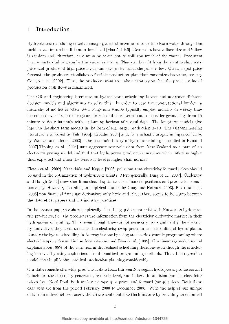
1 Introduction

Hydroelectric scheduling entails managing a set of inventories so as to release water through the

turbines at times when it is most bene�cial [Massé, 1946]. Reservoirs have a �xed size and in�ow

is random and, therefore, care must be taken not to spill too much of the water. Producers

have some �exibility given by the water reservoirs. They can bene�t from the volatile electricity

price and produce at high price levels and save water when the price is low. Given a spot price

forecast, the producer establishes a feasible production plan that maximizes its value, see e.g.

Conejo et al. [2002]. Thus, the producers want to make a strategy so that the present value of

production cash �ows is maximized.

The OR and engineering literature on hydroelectric scheduling is vast and addresses di�erent

decision models and algorithms to solve this. In order to ease the computational burden, a

hierarchy of models is often used: long-term studies typically employ monthly or weekly time

increments over a one to �ve year horizon and short-term studies consider granularity from 15

minute to daily intervals with a planning horizon of several days. The long-term models give

input to the short term models in the form of e.g. target production levels. The OR/engineering

literature is surveyed by Yeh [1985], Labadie [2004] and, for stochastic programming speci�cally,

by Wallace and Fleten [2003]. The economic theory of hydro scheduling is studied in Førsund

[2007].Tipping et al. [2004] uses aggregate reservoir data from New Zealand as a part of an

electricity pricing model and �nd that hydropower production increases when in�ow is higher

than expected and when the reservoir level is higher than normal.

Fleten et al. [2002], Näsäkkälä and Keppo [2008] point out that electricity forward prices should

be used in the optimization of hydropower plants. More generally, Ding et al. [2007], Caldentey

and Haugh [2006] show that �rms should optimize their �nancial positions and production simul-

taneously. However, according to empirical studies by Guay and Kothari [2003], Bartram et al.

[2006] non �nancial �rms use derivatives only little and, thus, there seems to be a gap between

the theoretical papers and the industry practices.

In the present paper we show empirically that this gap does not exist with Norwegian hydroelec-

tric producers, i.e. the producers use information from the electricity derivative market in their

hydropower scheduling. Thus, even though they do not necessary use signi�cantly the electric-

ity derivatives they seem to utilize the electricity swap prices in the scheduling of hydro plants.

Usually the hydro scheduling in Norway is done by using stochastic dynamic programming where

electricity spot price and in�ow forecasts are used Fosso et al. [1999]. Our linear regression model

explains about 88% of the variation in the realized scheduling decisions even though the schedul-

ing is solved by using sophisticated mathematical programming methods. Thus, this regression

model can simplify the practical production planning considerably.

Our data consists of weekly production data from thirteen Norwegian hydropower producers and

it includes the electricity generated, reservoir level, and in�ow. In addition, we use electricity

prices from Nord Pool, both weekly-average spot prices and forward (swap) prices. Both these

data sets are from the period February 2000 to December 2006. With the help of our unique

data from individual producers, the article contributes to the literature by providing an empirical

2

Electronic copy available at: http://ssrn.com/abstract=1344725

analysis of how commodity storage is operated in a situation where well-functioning markets for

spot and forward transactions are available.

Empirical and theoretical dynamics of commodity storage was pioneered by Kaldor [1939], Work-

ing [1949], Brennan [1958] and Telser [1958]. These explain how equilibrium inventories relate to

competitive spot- and futures prices and perform empirical analyses on agricultural commodities

such as cotton and wheat by using aggregate inventory data. High convenience yield is main

reason for holding inventory, it is a �ow of implicit value that accrues to those who hold the

commodity. Agricultural commodities are relevant in the context of electricity, since they are

perishable. However, electricity is a �ow commodity that can not be stored, so convenience yield

need to be interpreted as the bene�t of delivering it sooner rather than later. The relationship

between commodity storages and price volatility has been studied in several papers, see e.g. Ge-

man and Nguyen [2005] and the references there. Geman and Nguyen [2005] show that soybean

price volatility rises when the aggregate soybean inventory falls. Thus, when "scarcity" is high

then the price uncertainty is also high. Fama and French [1987, 1988] and Litzenberger and

Rabinowitz [1995] show that rising price volatility decreases inventories. Fama and French [1987,

1988] and Litzenberger and Rabinowitz [1995] use a proxy for inventories.

The remainder of this article is structured as follows. The institutional background is explained

in Subsection 1.1. Reservoir operations is the topic of Section 2, and Section 3 explains the data.

Section 4 displays the regression results, and Section 5 concludes.

1.1 Nordic Electricity Market

The consumption of electricity in the Nordic countries is characterized by seasonal variation,

mainly due to a high degree of direct electrical heating. Low temperatures and short day-lengths

lead to higher consumption in the winter than in the summer [Johnsen, 2001].

The Nordic power market, particularly the Norwegian part, is hydropower dominated. In Norway

almost 99% of electricity generation comes from hydropower, and in the whole of the Nordic

region hydropower constitutes over 50% of the power production [Nordel, 2007].

Norway has a water reservoir capacity of about 84 TWh which roughly constitute 70% of annual

generation in Norway. This gives the producers some degree of �exibility and the possibility to

schedule generation to the periods with the highest electricity prices. Retailers who buy in the

market and deliver electricity to the consumers naturally do not have this opportunity.

Limitations in reservoir capacities and variation in precipitation contribute to price variations

between seasons. Since most of the in�ow comes during late spring and summer when the snow

in the mountains melts, the reservoir capacity is sometimes not su�cient: The limited storage

capacity makes it impossible to transfer enough water into the winter season which normally

faces high demand and low in�ow. Due to the constraints the plants must produce at high level

during summer time in order to avoid costly spillage from over�ow in the reservoirs [Fleten and

Lemming, 2003].

3

Nord Pool ASA is the Nordic power exchange. It has developed from being solely a Norwe-

gian power exchange to be a multinational exchange for electrical power which serves Denmark,

Finland, Sweden and Norway. In addition to being an exchange, Nord Pool also publishes im-

portant market information such as total reservoir content in the Nordic countries and outages

for maintenance and repair.

In the Nordic market Elspot is the market for physical contracts and it is an auction-based

day-ahead market, where electrical power contracts are traded for each hour the following day.

About 70% of the Nordic consumption is traded at Elspot. The system price is the average of

the 24 hourly day-ahead prices calculated assuming no bottlenecks in the transmission grid. Its

annual volatility is about 189% [Lucia and Schwartz, 2000].

Nord Pool's Eltermin is the main Nordic marketplace for �nancial electricity contracts having

the Elspot price as the main underlying index. Popular products include futures contracts for the

next few weeks, and forward contracts for the next few months, quarters and years. Although

these are termed forwards at Nord Pool, they correspond best to textbook de�nition of swaps,

since they exchange a �oating electricity price with a �xed one [Benth et al., 2008]. There are

both baseload contracts and peak load contracts, where the latter is based on peak hours only,

i.e. from 8 am. to 8 pm. Baseload contracts are based on all 24 hours of the day. Other traded

products are European options, contracts for di�erences that pay o� depending on how much

di�erent area prices di�er from Elspot system prices, and futures/swaps for other underlying

indices such as the German EEX electricity price, the Dutch APX price, and CO2 emission

derivatives.

The forward curve captures the risk adjusted expected value of the future spot price. According

to e.g. Lucia and Schwartz [2000], the seasonal systematic pattern throughout the year is of

crucial importance in explaining the shape of the forward curve. The shape of the forward curve

displays one peak and one valley per year, in total accordance with the behavior of the system

price. The trade in �nancial contracts is more than four times the energy load in the Nordic

area.

The Norwegian Water Resources and Energy Directorate (NVE) collects continuous water level

data from almost 600 metering locations all over the country. This information is recorded in

the national database Hydra II and is used in their power and �ood forecasts [Engeset et al.,

2003]. Some of this information is publicly available; Svensk Energi, Nord Pool and NVE publish

water reservoir statistics regarding the percentage �lling in three zones of Norway and the whole

of Sweden. The statistics are published on a weekly basis and gives the producers important

information on the hydrologic balance in Scandinavia.

2 Hydropower Scheduling

Hydropower plants typically have quite complex topologies with several cascaded reservoirs or

power stations in the same river system. We will focus on simple topologies with no hydraulically

coupling to other stations. Hence, when the term hydropower station is used in this article, it is

4

assumed to be a hydropower station with only one reservoir connected to it1.

2.1 Power Generation

The process of generating hydroelectric power is quite simple and involves converting the kinetic

energy in the moving water into mechanical energy by the turbines. Then in turn the turbines

spin a generator rotor which produces electrical energy. The power generated at the hydropower

station is generally a nonlinear function of water release and the station's net head which is the

di�erence between the headwater elevation and the tail water elevation. The release of water is

in turn a function of the volume of the reservoir.

Depending on the size of the reservoir and the time horizon, it is sometimes reasonable to make

the assumption that there is a �xed energy coe�cient, saying how many kWh of electricity one m3

of water produces. This approximation is standard in long-term scheduling and in systems where

production is a near linear function of release, e.g., because the head variation is small compared

to the average head [Lamond and Sobel, 1995]. We will use this approximation throughout.

Due to the Nordic power market's dependence on hydropower, the reservoir content and the in�ow

to the reservoirs are factors that are expected to in�uence the market prices and the electricity

production. Therefore, producers follow regularly information on these variables [Johnsen, 2001].

Naturally, the in�ow is expected to increase the production. Furthermore, seasonal variation may

a�ect how the production decision depends on in�ow.

Since water can be lost through over�ow, it is important to model in�ow as a stochastic variable.

In Norway there are long time series of historical observed in�ow from a large amount of metering

locations that enables in�ow analysis. The risk of over�ow is particularly considerable when the

snow melts in the spring. This risk can be reduced if the producer has information about the

snow reservoir. Then the future in�ow will consist of a known part, the melted snow, and an

unknown part, the future precipitation minus possible evaporation [Hindsberger, 2005]. Many

producers follow all these factors and try to forecast them in order to improve their production

scheduling.

2.2 Production Factors

There are several factors that a�ect the hydropower scheduling. First, if the expected future

electricity price is high relative to the current spot price then it is optimal to postpone the

production (see e.g. [Näsäkkälä and Keppo, 2008]). Thus, price forecasts are needed in estimating

the water values and the optimal production strategy.

Second, we expect that a positive deviation from the average reservoir level results in increased

production. Furthermore, when a reservoir is nearly empty or nearly full, the in�ow is the main

driver in the production decisions and electricity prices do not a�ect the decisions signi�cantly.

1If there are more than one reservoir connected to the power station(s), we aggregate the system into one

equivalent reservoir and power station.

5

Third, if there is an unexpected increase in the spot price or in�ow volatility then, by the real

option theory [Dixit and Pindyck, 1994], we expect a decrease in the production since the value

of waiting for more information is high.

From the above discussion we can form the following hypotheses on the hydropower scheduling:

• If the expected future prices are high relative to the current spot price then the current

production is low.

• Electricity production rises in reservoir level.

• Electricity production falls in electricity price and in�ow volatilities.

These hypotheses are studied more in the empirical analysis. Before that we next introduce the

data used.

3 Data

The empirical analysis presented in this paper is mainly based on data from thirteen Norwegian

hydropower producers. The selected producers are introduced in Table 1. The power stations

have di�erent production capacity, reservoir size and other physical conditions. For example, the

smallest producer has a capacity of 23 MW and the largest producer has a capacity of 210 MW.

Table 1: Descriptive data from the thirteen hydropower plants. Some notion require clari�cation; In�ow

is the expected yearly in�ow, relative regulation is de�ned as reservoir size divided by annual expected

in�ow and capacity factor is de�ned as annual expected in�ow divided by the rated power station capacity.

Here the capacity factor is given as a percentage of a year.

Rated Energy Reservoir Annual Relative Capacity

Producer capacity coe�cient size in�ow regulation factor

[MW] [kWh/m3] [GWh] [GWh/yr] [yr] [%]

1 128 1.16 228.1 641.2 0.356 57.2

2 120 1.32 624.4 380.8 1.640 36.2

3 30 1.15 47.1 106.6 0.442 40.5

4 40 1.27 51.8 139.9 0.370 39.9

5 28 0.67 118.9 87.8 1.350 35.8

6 23 0.16 14.0 153.0 0.092 76.0

7 68 1.25 255 272.3 0.937 45.7

8 167 1.09 272.5 414.4 0.642 28.3

9 210 1.46 1270 1250.5 1.015 68.0

10 62.1 1.50 142 231.8 0.613 42.6

11 41 0.95 42.6 81.3 0.953 22.6

12 29 0.91 12.4 147.2 0.084 57.9

13 140 1.36 380.8 662.9 0.574 54.0

6

In the modeling of the producers we make the following assumption:

• All the producers are price takers. That is, the producers are small relative to the aggregate

market volume and, therefore, they are not able to a�ect the market prices.

• If the producers have bilateral contracts that obligate them to deliver power to a contracted

price, they can purchase the contracted volume at the spot market. Therefore, the contracts

do not change the scheduling problem.

To comply with the assumption that the producers act as price takers the largest producers in

Norway such as Statkraft and Hydro are not included in our data set. Further, all the companies

in Table 1 are producers that participate in the Nordic electricity market. Therefore, for instance

industrial companies that produce for their own consumption are not considered. In our data set

there are no run-of-the-river plants because they are not as �exible as producers with reservoirs.

In addition, to keep the focus on external factors the power stations in Table 1 do not have water

connections to other stations that a�ect the production considerably.

3.1 Producer Panel Data

We have weekly data on the thirteen producers, from February 2, 2000 to December 27, 2006,

which totals 361 data points. The producer data includes production, reservoir level and in�ow

time series. Some of the producers do not directly measure in�ow, but calculate it using the

change in reservoir level, production and spill. Thus, with these producers the in�ow time series

is estimated based on their data. Since the data from the di�erent producers have the same time

horizon, our data set is a balanced panel data set.

The data from the thirteen producers was gathered through electronic correspondence. We have

avoided to alter the time series. In some in�ow time series a few data points were negative. Since

this is clearly unrealistic and caused by an error in measurements or calculations, these values

were set equal to zero. A transformation of the reservoir level data with denomination Mm3 to

MWh using the average energy coe�cient was required for some producers. In addition, some

of the data we received was on hourly or daily basis. In these cases, we aggregated the data so

that it has the form MWh/week or MWh.

3.2 Production Data

In Figure 3.1 the weekly relative production, i.e., the weekly production divided by the maximum

weekly production for the producers is plotted against time. As can be seen, the relative pro-

duction varies considerably. A tendency of an annual periodical trend can be noticed. Further,

quite often the data shows zero production over a week. This may be due to the fact that the

producer �nds it unfavorable to generate or there is maintenance or a breakdown. Unfortunately,

information concerning planned and unplanned production interruptions is not available for the

7

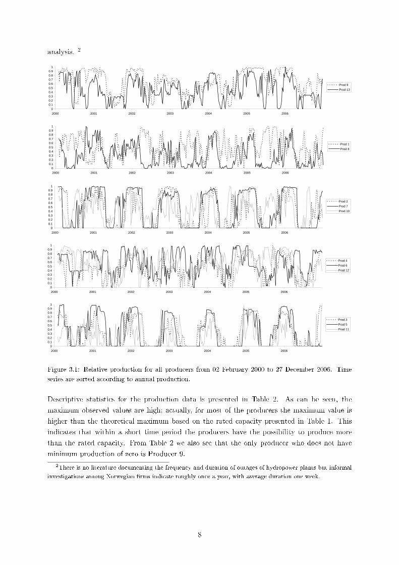
analysis. 2

0.82621821 0.01735324 0.15912475 0.77237583 0 0.38549265 0.19183029 0.04839812 0.87310136 0 0.43863571 0.89325651 0.187471350.83445034 0 0 0.81666003 0 0.38802395 0.15127832 0.05435773 0.91297717 0.41116337 0.31047854 0.78632096 0.060267480.73216028 0 0 0.68407616 0 0.02305389 0.0370716 0.07755087 0.754669 0.46438931 0.26394781 0.753137 0

0.4359685 0.01809167 0 0.03434175 0 0.24733261 0 0 0.44207709 0.4075962 0.15697277 0.86944089 00.60871039 0 0 0 0 0.39011976 0 0.00060735 0.16499551 0.58895867 0.16792117 0.85753308 0.770181260.73631987 0 0 0 0 0.39060969 0 0.42252505 0.14821575 0.79529133 0.02431458 0.68309859 0.53420147

0.5901022 0 0 0 0 0.39915623 0.36641574 0.45269131 0.1321181 0.81641274 0.00010644 0.30766112 0.885896180.483932 0 0 0.000627 0 0.39812194 0.66347705 0.09425296 0.15830544 0.92117491 0 0.69630815 0.90843657

0.56338557 0 0 0 0.17327208 0.40285792 0.21286952 0.24559672 0.12253317 0.93581909 0.14175144 0.89029023 0.523983160.88513956 0 0 0.1672839 0.47406557 0.3955362 0 0.31965533 0.32936894 0.85030086 0.49397077 0.89502774 0.829969390.76687083 0 0 0.24870448 0.46504489 0.39199782 0.54823234 0.27824172 0.52810951 0.91619965 0.18826696 0.90157917 0.912529980.83627818 0.19874466 0.40330571 0.1656537 0.4785759 0.22014154 0.34756592 0.2310082 0.82680287 0.73483718 0.19885042 0.86980367 0.912590850.89753586 0.39089614 0 0.24178955 0.031635 0.39161677 0.34426873 0.2842393 0.92162625 0.61665118 0.23052476 0.85394793 0.31100408

0.7149768 0.49839127 0 0.48343579 0.25489664 0.39131737 0.41690291 0.37043425 0.95281477 0.73080064 0.51737299 0.82106274 0.398943930.71696039 0.82942138 0.0038653 0.79826202 0.47350177 0.39564507 0.55352704 0.34455664 0.95187347 0.72300919 0.34609127 0.91205719 0.530248820.61981942 0.57550504 0 0.44044143 0.45011485 0.39853021 0 0.20638476 0.96628496 0.69616154 0.35156547 0.65153649 0.29303264

0.7281931 0.36162772 0.08315299 0.17020394 0.47584047 0.40865542 1.7445E-05 0.17654874 0.97095328 0.32433092 0.53814455 0.42880922 0.308219350.89021994 0.44902157 0 0.42727441 0.47089163 0.86856287 0.68191691 0.38194655 0.9722029 0.46082214 0.45233642 0.43474178 0.294124470.56664727 0.50356031 0 0.40683417 0.44773439 0.85108873 0.65825214 0.85085788 0.909111 0.21637707 0.65226647 0.55911225 0.358066890.12964804 0.54480722 0 0.40755074 0.4534976 0.8595264 0.95053339 1 0.62750025 0.58726896 0.22827426 0.61158771 0.013820970.13566753 0.77488264 0.51010177 0.40658337 0.21524327 0.8729178 0.95812217 0.97399787 0.68750904 0.59900307 0.32367745 0.5530303 00.15767485 0.76512474 0.53035045 0.39966844 0.17001462 0.82830702 0.81787811 0.57288187 0.75703181 0.36094136 0.35418092 0.53045241 0.047302480.09116271 0.65979218 0.39325986 0.41104403 0.46784297 0.8312466 0.69449508 0.50140449 0.7981163 0.47368273 0.12643888 0.68141272 0.118100220.19825371 0.74756053 0.35807975 0.41727822 0.85433285 0.84931954 0.76196541 0.66690708 0.94385738 0.78872023 0.38086766 0.49553991 0.49560320.15478879 0.63531832 0.40040183 0.4297645 0.50780956 0.84041916 0.93981316 0.35085788 0.94577273 0.72929868 0.30579505 0.36286812 0.575557850.16774856 0.68452977 0.45877374 0.5595179 0.38429735 0.85696788 0.9660773 0.50603553 0.93877434 0.68733748 0.17791159 0.84046095 0.63638456

0.1012914 0.6390105 0.24474996 0.48603337 0.49310921 0.86208492 0.74301091 0.45346189 0.9222265 0.48701268 0.05305415 0.8681178 0.638518760.0940167 0.5833641 0.42437846 0.49918248 0.92555857 0.8306478 0.96295456 0.52550865 0.93308559 0.57149831 0.02668674 0.87763551 0.674739360.4002318 0.77409146 0.61954664 0.47773904 0.96600543 0.85264017 0.99094581 0.79448831 0.96951541 0.46354445 0.34114928 0.92180965 0.72042882

0.38707505 0.82251174 0.45512427 0.18548485 0.97987054 0.66750136 0.99323988 0.78211357 0.97699127 0.33747313 0.23163481 0.90943235 0.642775760.13757324 0.74766602 0.43950611 0.43146636 0.97826269 0.83230811 1 0.77273763 0.87614082 0.40553099 0.17043018 0.87887324 0.63996820.40507396 0.7959808 0.74288304 0.50391186 0.97759449 0.87093087 0.99631901 0.87412694 0.97849462 0.79378937 0.27565652 0.70614597 0.742204540.46983614 0.94514479 0.85138611 0.51277945 0.97872207 0.68753402 0.97944925 0.91360462 0.98209886 0.78243075 0.3565987 0.79553991 0.82637435

0.4448374 0.82836648 0.72844213 0.45618812 0.97911881 0.83089276 0.97977199 0.60795627 0.85644438 0.57159218 0.19290482 0.61969697 0.726329260.81257129 0.91682051 0.74655213 0.49837634 0.97861767 0.87591181 0.98477011 0.80906468 0.955314 0.74779164 0.61227438 0.86160905 0.726089590.61167432 0.86866396 0.63173116 0.48460022 0.72413865 0.71211214 0.9900212 0.90965685 0.91628673 0.66828128 0.20943388 0.76440461 0.61377570.39729535 0.43472757 0.76479949 0.2743757 0.84222176 0.76586826 0.99282992 0.65548132 0.7381157 0.51404808 0.00437936 0.35620999 0.297209750.79735307 0.7158078 0.47921862 0.36074063 0.95644185 0.63247142 0.70750068 0.76328576 0.88494269 0.69494119 0.40603379 0.45151515 0.465739560.91289151 0.96592647 0.42861656 0.44312858 0.95573189 0.68669026 0.80474168 0.89644701 0.98342487 0.73408619 0.52158509 0.73269313 0.569417740.56268467 0.94424811 0.39145475 0.42637869 0.95472959 0.60266739 0.98889596 0.42298056 0.91730989 0.49226957 0.02843544 0.55349979 0.42475220.73900436 0.66348436 0.32156543 0.44823416 0.85429108 0.40419162 0.98608724 0.50269511 0.78801025 0.3611291 0.07434272 0.58371746 0.36260540.73730479 0.87409674 0.35258592 0.47179149 0.83936104 0.5578933 0.98060937 0.45851048 0.92391811 0.25298751 0.09316789 0.75964575 0.410516560.39787256 0.77388048 0.35150678 0.17728009 0.82405513 0.33639085 0.98433398 0.32064227 0.92848003 0.24923259 0.02034579 0.04314981 0.320499580.31120843 0.58257292 0.34887759 0.0249009 0.83322197 0.73026674 0.98324363 0.30795589 0.87396627 0.24960808 3.0412E-05 0 0.34857520.15044596 0.43446384 0.2111199 0 0.83253289 0.90321176 0.98017323 0.25075919 0.89822462 0.04017761 0.04307893 0 0.332912960.26912241 0.73980695 0.25877884 0.11680136 0.81250783 0.88111051 0.97553274 0.10047829 0.84336708 0 0.2238949 0 0.350268110.10693524 0.63283928 0.32093756 0.14116483 0.76621424 0.86741971 0.79642891 0.14687139 0.76702873 0.0270354 0.11401548 0 0.22347510.08553261 0.1334986 0.31193161 0.40328713 0.57371059 0.86597714 0.06104167 0.14614333 0.55341284 0 0 0 0.011781870.21446143 0.19114932 0.28385423 0.29275579 0.27529756 0.88323353 0.035266 0.02266171 0.3384764 0.1902804 0 0 0.007844440.16130303 0.12384619 0.02778306 0 0 0.88062058 0 0 0.26841613 0.22116459 0 0.09620145 0.069911340.27549464 0.19821721 0 0.08584541 0 0.84828525 0 0 0.28298587 0.23045801 0 0.8103073 0.280227420.34742614 0.19489425 0 0.27014792 0 0.34447469 0 0.12408898 0.40501428 0 0 0.71777636 0.05081383

0 0.00838652 0 0.41872928 0 0.30963527 0 0.4155785 0.32764459 0.00018775 0 0.57437047 0.123399580 0.01334459 0 0.47433532 0.44182502 0.35340229 0.0074841 0.53241725 0.40156829 0.28950407 0 0.51320956 0.28815935

0.17026813 0 0.09949712 0.36693898 0.1299645 0.33091998 0 0.50584573 0.26930286 0.1247571 0 0.17471191 0.037304820.29692475 0 0 0 0 0.0095264 0 0.56145612 0.26581049 0.15085377 0 0.04953052 0.012405770.47217247 0 0 7.1657E-05 0 0 0 0.43452019 0.28762145 0.24838773 0 0.37055058 0.198534210.29751112 0 0 0 0 0.17463255 0 0.28074704 0.18839987 0.24031466 0 0.12985489 0.22166046

0.436477 0 0 0 0 0.4086282 0.11766964 0.60103477 0.0607018 0.23411905 0 0.04361929 0.294006540.83089088 0 0 0 0 0.25988024 0.34458275 0.48151382 0.06134025 0.26763168 0.00708605 0 0.29324188

0.7704303 0 0 0 0 0.07724551 0.71416484 0.40092165 0.13800056 0.72526214 0.08364886 0.06895006 0.27487099

00.10.20.30.40.50.60.70.80.9

1

2000 2001 2002 2003 2004 2005 2006

Prod 9Prod 13

00.10.20.30.40.50.60.70.80.9

1

2000 2001 2002 2003 2004 2005 2006

Prod 1Prod 8

00.10.20.30.40.50.60.70.80.9

1

2000 2001 2002 2003 2004 2005 2006

Prod 2Prod 7Prod 10

00.10.20.30.40.50.60.70.80.9

1

2000 2001 2002 2003 2004 2005 2006

Prod 4Prod 6Prod 12

00.10.20.30.40.50.60.70.80.9

1

2000 2001 2002 2003 2004 2005 2006

Prod 3Prod 5Prod 11

Figure 3.1: Relative production for all producers from 02 February 2000 to 27 December 2006. Time

series are sorted according to annual production.

Descriptive statistics for the production data is presented in Table 2. As can be seen, the

maximum observed values are high; actually, for most of the producers the maximum value is

higher than the theoretical maximum based on the rated capacity presented in Table 1. This

indicates that within a short time period the producers have the possibility to produce more

than the rated capacity. From Table 2 we also see that the only producer who does not have

minimum production of zero is Producer 9.

2There is no literature documenting the frequency and duration of outages of hydropower plants but informal

investigations among Norwegian �rms indicate roughly once a year, with average duration one week.

8

Table 2: Descriptive statistics for production data. The variables are in MWh/week. ADF is the

Augmented-Dickey-Fuller test statistic having a critical value of -2.87 at a 5% signi�cance level [Dickey

and Fuller, 1979].

Producer Mean Min Max Std. dev ADF

1 11059 0 21829 5900 -7.583

2 7755 0 18959 7199 -4.441

3 1697 0 5097 1642 -3.820

4 2448 0 5582 1610 -5.333

5 1734 0 4789 1808 -3.949

6 2141 0 3674 1039 -6.539

7 5327 0 11464 4771 -4.132

8 7963 0 26344 7059 -6.086

9 23835 1985 36651 10130 -4.744

10 4662 0 10653 3090 -6.465

11 1448 0 6576 1669 -7.242

12 2616 0 4686 1343 -6.769

13 11863 0 26286 7176 -6.380

3.3 Reservoir Data

Figure 3.2 illustrates the relative reservoir content, i.e., reservoir content as a percentage of

the maximum reservoir capacity. A clear periodical variation can be seen. Since many of the

reservoirs are emptied once a year, it may be argued that the producers use production scheduling

conditional that the reservoirs are at their minimum level at the given date. This agrees with the

fact that all of the producers in our sample have a rather low relative regulation. The reservoir

data is used in Section 4.1.

3.4 In�ow Data

In�ow time series (weekly in�ow in MWh/week) is illustrated in Figure 3.3. It is expected that

there are some seasonal variations over a year. However, due to the variations between the years

(some of the years are �wetter� than the others), this e�ect is not clear in the �gure. There seems

to be signi�cant di�erences of the spread of in�ow during a year. Some of the producers have

evenly spread in�ow, while others have periods with high and/or low in�ow. This is also evident

from Table 4 where descriptive statistics for the in�ow data is presented.

3.5 Spot Price Data

Electricity price data is obtained from Nord Pool (www.nordpool.com). What we call spot prices

in the analysis are weekly average day-ahead system prices in Euro/MWh. Due to the averaging

we do not have hourly and daily price variations in our data. In the �rst row of Table 5 the

descriptive statistics of the spot price are presented.

9

0.42292521 0.70354901 0.48619958 0.21561875 0.74094449 0.81198917 0.09622549 0.2145424 0.35385827 0.13661972 0.54207918 0.794322580.35277729 0.67691224 0.44373673 0.16264826 0.7127132 0.86410097 0.04980392 0.17577179 0.34551181 0.1028169 0.50687241 0.772258060.33326629 0.65344651 0.40339703 0.12041884 0.67608579 0.8353093 0.00019608 0.14014948 0.32700787 0.06267606 0.457016 0.757548390.26892582 0.62892377 0.36942675 0.10716408 0.64069807 0.77592301 0.00235294 0.11255609 0.31771654 0.04788732 0.44465167 0.757548390.21034187 0.60651505 0.30785563 0.07149584 0.60063331 0.71281835 0.00401961 0.11288767 0.29527559 0.03028169 0.40711824 0.713419350.15252205 0.58030109 0.25690021 0.04305015 0.56310429 0.62210858 0.00539216 0.08985418 0.27653543 0.01901408 0.34895288 0.639870970.09648523 0.55746957 0.22292994 0.03121116 0.54490328 0.64148363 0.00642157 0.07833412 0.26661417 0.01197183 0.25673656 0.489096770.05700473 0.53210122 0.23991507 0.11016357 0.52608242 0.73624437 0.0077451 0.08708674 0.24307087 0.01478873 0.21577378 0.419225810.0510954 0.50736707 0.26963907 0.17262088 0.51689739 0.87746439 0.01171569 0.19466561 0.30858268 0.01549296 0.28491595 0.39716129

0.05736133 0.49891095 0.3014862 0.24592433 0.52698402 0.90358919 0.03186275 0.38143194 0.36125984 0.01126761 0.39832975 0.367741940.08680614 0.48876361 0.30785563 0.28710196 0.55098907 0.81795451 0.08617647 0.51012702 0.39149606 0.00704225 0.55590576 0.389806450.20030618 0.50165919 0.35456476 0.37977238 0.57617746 0.70256945 0.20367647 0.59142249 0.43582677 0.03873239 0.70140004 0.481741940.26755037 0.52696624 0.40127389 0.40157008 0.6232296 0.63116934 0.33877451 0.64282739 0.45653543 0.13802817 0.78583356 0.508219350.32638904 0.55996413 0.47346072 0.42133774 0.63461228 0.71178853 0.38485294 0.6971083 0.47645669 0.2084507 0.85671521 0.511161290.34773398 0.58196272 0.48619958 0.43928971 0.63686627 0.76948426 0.41401961 0.71603093 0.48582677 0.28239437 0.87548843 0.459677420.47768847 0.60896099 0.5626327 0.57107935 0.64413541 0.74877103 0.44941176 0.72719126 0.51527559 0.33098592 0.90654865 0.507483870.59098474 0.63595926 0.60509554 0.62680057 0.73294281 0.72605286 0.48960784 0.74102573 0.53897638 0.3971831 0.93757863 0.661935480.71176957 0.70795464 0.63057325 0.71820584 0.74731203 0.77293074 0.57553922 0.81020223 0.55283465 0.59295775 0.95258081 0.650903230.78848908 0.74595221 0.64118896 0.77068569 0.77300757 0.76244228 0.68357843 0.9281405 0.56629921 0.64929577 0.95472769 0.58838710.82934502 0.7929492 0.64543524 0.81221649 0.79216653 0.79446639 0.75372549 0.95892095 0.58149606 0.75140845 0.95164897 0.58838710.85787286 0.83894625 0.64755839 0.82405838 0.80833894 0.86846368 0.81573529 0.94456556 0.59448819 0.8528169 0.96765442 0.77078710.87723104 0.86994427 0.64968153 0.84623107 0.83916232 0.86788831 0.83897059 0.95818206 0.60070866 0.86338028 0.97430005 0.870077420.86704253 0.89094292 0.66029724 0.86940817 0.87522624 0.87848834 0.85441176 0.95929051 0.60677165 0.85070423 0.97187871 0.920090320.88130644 0.93993978 0.69002123 0.94109942 0.89770984 0.830815 0.87044118 0.94603277 0.61212598 0.93591549 0.98449385 0.941419350.86755195 0.96193837 0.74097665 0.93882339 0.89044071 0.79401839 0.88794118 0.94053681 0.61897638 0.93169014 0.98487725 0.963483870.85481631 0.97493754 0.74522293 0.95879688 0.916418 0.87207586 0.89284314 0.95892095 0.61661417 0.92816901 0.96627725 0.963483870.80693029 0.98093716 0.76220807 0.94425726 0.92233474 0.88702687 0.90171569 0.96039962 0.60433071 0.9471831 0.96437984 0.956129030.84513722 0.97993722 0.81316348 0.96047632 0.94138099 0.86870778 0.9104902 0.96410142 0.59913386 0.93943662 0.91078024 0.989225810.8466655 0.9709378 0.8343949 0.90804591 0.97603616 0.9061961 0.92490196 0.95191334 0.57944882 0.93450704 0.89533819 0.85904516

0.80693029 0.96793799 0.84501062 0.87179207 0.97361312 0.9521272 0.91730392 0.94860321 0.55480315 0.93450704 0.86645416 0.801677420.75598772 0.97293767 0.8492569 0.86855496 0.96876703 0.95366508 0.94166667 0.95301804 0.53566929 0.93732394 0.78189735 0.800941940.67957387 0.96993786 0.86199575 0.84097945 0.96702019 0.96733223 0.97686275 0.94493225 0.51511811 0.92676056 0.71780128 0.792116130.64773477 0.96593812 0.87261146 0.80161599 0.9625122 0.98298332 0.97230392 1.01061415 0.50582677 0.93732394 0.62926834 0.809032260.65614029 0.96393824 0.90658174 0.7668855 0.95107317 0.95918451 0.98019608 1.01365376 0.50874016 0.91338028 0.55326009 0.767109680.67244191 0.93893985 0.91082803 0.75383735 0.96358284 0.93978838 0.99529412 0.98421812 0.52401575 0.88028169 0.52205974 0.6840.66887593 0.90894177 0.91507431 0.74233298 0.95524306 0.94741201 0.97073529 0.98796694 0.53566929 0.85915493 0.47832954 0.675174190.66592126 0.89694254 0.89384289 0.71124005 0.93828175 0.90630319 0.9522549 0.98721659 0.5280315 0.82676056 0.44174672 0.584709680.65053661 0.87294407 0.87048832 0.6722235 0.90847267 0.93775629 0.93656863 0.96929629 0.51598425 0.76760563 0.41150252 0.592064520.64187637 0.85494523 0.84713376 0.63197619 0.87731119 0.97128527 0.91490196 0.97338808 0.5011811 0.71197183 0.35415724 0.529548390.64493292 0.84094612 0.83227176 0.60139894 0.85927923 0.96191813 0.88470588 0.95522943 0.49968504 0.66408451 0.31855647 0.452322580.67193249 0.82394721 0.8641189 0.57900617 0.86096972 0.96621594 0.85235294 0.95117724 0.49795276 0.63309859 0.31491049 0.415548390.67371548 0.8069483 0.88322718 0.56101077 0.87556434 0.98063461 0.83088235 0.93651694 0.49519685 0.59647887 0.32064519 0.404516130.63657834 0.78294984 0.82590234 0.52675894 0.88458032 0.98733556 0.79573529 0.8808185 0.4719685 0.56690141 0.30317915 0.378774190.60107137 0.76995067 0.78980892 0.51533665 0.80867704 0.9070649 0.75470588 0.82585854 0.44692913 0.54647887 0.26706241 0.364064520.59062815 0.74395234 0.75159236 0.4738536 0.76523129 0.80908152 0.71343137 0.76943182 0.42527559 0.50211268 0.22484052 0.3420.56566629 0.7289533 0.67940552 0.42661458 0.74026829 0.79777094 0.67392157 0.70118576 0.39929134 0.44225352 0.1991608 0.364064520.54890618 0.69795529 0.59447983 0.37140425 0.70257023 0.70547806 0.63181373 0.62554108 0.37307087 0.4056338 0.15323912 0.353032260.52318018 0.67495676 0.53927813 0.32192434 0.66289992 0.64179858 0.58691176 0.5802731 0.3511811 0.3471831 0.11642667 0.355238710.45313415 0.64895842 0.46496815 0.28322646 0.63145669 0.67172285 0.54534314 0.50667892 0.32574803 0.2943662 0.07926899 0.257419350.39913503 0.62296009 0.40976645 0.23825985 0.59088478 0.57384734 0.50416667 0.4332308 0.30220472 0.2471831 0.02902198 0.147096770.55384761 0.61296073 0.35031847 0.24798799 0.57589571 0.48535263 0.46343137 0.37486915 0.28653543 0.20915493 0.06103194 0.13238710.4778413 0.59596182 0.32271762 0.23871692 0.52946341 0.40085996 0.42034314 0.30979137 0.27023622 0.16549296 0.10595668 0.16180645

0.38894651 0.56896355 0.2866242 0.20401082 0.49880908 0.30850008 0.39156863 0.22388927 0.24188976 0.11338028 0.03564079 0.136064520.3469189 0.54196528 0.27813163 0.16032086 0.45637763 0.18827036 0.35333333 0.19311186 0.21716535 0.08028169 0.01990159 0.14709677

0

0.2

0.4

0.6

0.8

1

2000 2001 2002 2003 2004 2005 2006

Prod 9Prod 13

0

0.2

0.4

0.6

0.8

1

2000 2001 2002 2003 2004 2005 2006

Prod 1Prod 8

0

0.2

0.4

0.6

0.8

1

2000 2001 2002 2003 2004 2005 2006

Prod 2Prod 7Prod 10

0

0.2

0.4

0.6

0.8

1

2000 2001 2002 2003 2004 2005 2006

Prod 4Prod 6Prod 12

0

0.2

0.4

0.6

0.8

1

2000 2001 2002 2003 2004 2005 2006

Prod 3Prod 5Prod 11

Figure 3.2: Reservoir content for all producers from week 5 in 2000 until week 52 in 2006.

10

Table 3: Descriptive statistics reservoir data. All data are in MWh. ADF is the Augmented-Dickey-Fuller

test statistic having a critical value of -2.87 at a 5% sign. level.

Producer Mean Min Max Std. dev ADF

1 135517 558 208347 58219 -1.923

2 412736 183562 612497 109436 -1.334

3 25229 300 46900 12264 -1.180

4 28829 1617 51721 13620 -1.537

5 63145 0 119113 31008 -0.7387

6 8338 1242 13823 2897 -3.172

7 141294 50 253800 81101 -1.368

8 171573 5380 276221 87367 -1.570

9 433929 37500 786100 173834 -1.212

10 67641 100 135200 46670 -1.346

11 23491 400 41956 11203 -1.550

12 7359 0 12266 2621 -3.786

13 236639 15617 388839 114489 -1.328

Table 4: Descriptive statistics in�ow data. All data are in MWh/week. ADF is the Augmented-Dickey-

Fuller test statistic having a critical value of -2.87 at a 5% sign. level.

Producer Mean Min Max Std. dev ADF

1 11638.63 0 63125.10 12375.56 -8.820

2 7312.65 0 50556.00 9151.31 -6.058

3 1743.28 0 6860.34 1437.45 -11.25

4 2709.79 0 12063.05 2318.80 -8.951

5 1872.45 0 24083.89 2193.93 -12.98

6 2967.86 0 22342.42 3250.55 -8.376

7 5575.83 0 43000.00 7542.10 -6.666

8 8413.89 0 77892.03 11601.80 -7.876

9 24149.50 0 118600.00 22266.42 -9.825

10 4795.54 0 32790.00 6077.11 -6.456

11 1577.18 0 12780.18 1785.31 -11.73

12 2784.34 0 36409.64 3762.68 -9.312

13 13779.56 0 209859.60 27271.23 -7.281

11

6102.2 8900 3011.67648 1320 750 1083.71821 1690 1030.75921 2776.16585 4495.35744 800 572.3901883089.2 8900 1294.992 1320 1000 1904.59994 670 2127.57929 2472.21297 854.94528 1200 4518.3235

5173 13000 2957.57568 1056 750 983.562246 300 1864.22665 4355.39926 976.292352 1900 724.6743752705.4 25100 2143.07712 0 875 1161.04099 450 1996.03723 2771.44608 237.178368 1800 542.2612654849.4 12300 1809.8064 2508 625 739.254327 0 1639.08196 2481.6525 512.967168 1700 0

26448.4 20600 3328.49664 1980 375 1485.84914 1720 3198.94373 2977.22784 1577.51194 2000 992.44015413397 6500 1894.36032 924 500 644.387728 350 1754.59178 2644.01242 292.336128 500 127.5987887101.4 9700 3224.5056 264 375 572.507557 870 416.397017 3269.85328 518.482944 1300 162.9116995731.2 21900 5459.38272 396 625 1588.4943 70 697.881933 2919.64671 0 700 0

13463.6 6000 0 1452 1000 2385.08809 350 3279.92619 4703.71792 2619.9936 4700 1211.8910825684 118600 1579.30272 396 4625 29315.2423 430 7779.76872 3875.87112 3750.72768 4600 2952.7247723686 99600 3058.92288 3168 13625 51661.8034 220 8729.68246 2582.65548 6293.50042 3800 5043.7232128104 60100 0 4092 32500 35134.809 830 7987.55251 2063.48131 3949.29562 2700 5294.7422649998 78800 76293.6826 10560 35375 22218.4166 4900 9860.32989 1771.79983 14512.0067 4000 6490.1089

42950.6 52400 142309.486 17028 12000 14073.2359 14130 6096.51072 1475.39858 6602.38387 2600 3124.4950435757.2 50700 179256.122 20724 8125 14856.9473 9980 6005.61138 3498.28991 2719.27757 3400 2982.9455523333.8 43900 85857.1862 13992 9250 6501.51278 10460 5318.29282 1320.59028 6254.88998 1300 4054.8254643369.2 70900 28291.4381 17028 12000 4543.86517 11230 12063.0524 740.059172 11643.8031 3700 7822.25001

38301 57800 127613.604 24024 19625 5885.81627 14320 7053.15727 235.044303 9729.82886 2000 3587.8366737108.4 33800 127075.582 43032 23500 18915.9976 32150 5388.54015 1356.4605 8042.00141 1200 7386.7436

28862 23200 209859.598 23892 19000 32219.636 14250 2800.35 833.510521 15742.0247 500 2823.0431924583.4 24700 38990.0304 29040 14250 19625.0719 22930 2082.8 3306.66745 16806.5695 200 989.56631427114.4 21400 31618.1232 27984 9250 8123.18174 23100 552.45 1561.2983 10788.8579 100 3475.223

15706 13700 193826.03 18216 10250 6268.04093 11340 1115.02825 1386.66699 9801.53395 100 4450.146495.6 12200 165994.914 12540 6500 6861.28267 8140 1111.25 1360.23631 7413.20294 500 3338.15189

35503.6 18900 167022.927 29172 4000 4904.68244 21150 4525.9371 906.194904 5206.89254 1500 3101.9195618132.4 28100 201801.663 12672 6625 5924.74941 9130 1384.36985 1570.73783 5124.1559 2400 3178.5938617152.4 27400 32669.0986 11220 7250 11183.1739 7320 2039.61365 2054.04178 2272.49971 2300 3739.587510761.4 18200 12137.6246 10164 5875 7983.91643 9240 764.85115 963.776039 4671.86227 800 2834.632239816.2 28400 7866.74592 8844 7500 10868.8058 6640 3630.6887 1422.53721 5444.07091 2400 5043.61473

35192.6 9900 6895.67328 9108 4500 5854.58089 6970 2409.952 1683.06824 2289.04704 1000 2089.681686197.4 4200 3585.97728 8976 5500 4620.41334 7420 945.9087 4588.55566 1450.64909 500 1887.728134684.6 11300 3766.29696 8712 8125 5871.17435 3860 860.53295 5600.4733 1858.81651 600 979.3287781715.8 9600 3107.19744 6732 6875 7895.68291 3450 968.16545 4088.26055 1439.61754 600 867.965629

2699 21600 3767.81472 6600 9250 53475.8759 3820 610.0445 12740.534 1014.90278 500 548.0580351281.4 26700 2333.13984 7656 16000 31803.7249 2810 544.5125 8530.50349 590.188032 1600 4737.401816850.8 44600 1127.69568 0 7875 22724.497 1640 1529.2832 8669.26458 364.041216 2700 2933.73888206.2 42600 1985.5728 0 4375 16169.1415 870 2249.6145 22342.4242 391.620096 3000 2418.9273

0 19600 2447.06976 1320 3625 13053.181 490 768.76275 19499.2376 237.178368 1000 824.2834040 19300 1952.86752 0 2250 12750.4302 0 368.17935 15961.3017 330.94656 700 492.5862640 15900 2872.67904 264 2625 10392.0556 0 373.5705 21780.7721 165.47328 900 495.9006010 32600 2540.2896 3300 2500 8431.86989 480 1434.85235 11156.5808 16.547328 1700 2206.19441

2112.4 31600 2701.71072 924 2250 10885.7787 750 1552.65574 7923.54169 126.862848 2800 2652.60973742.6 30700 2353.40928 0 1875 9900.05969 900 2153.49818 11082.9525 209.599488 3000 0

0 6100 2120.84928 0 625 5829.26448 710 683.524886 3297.22792 38.610432 400 00 4100 2099.11104 6468 750 5703.30123 720 620.707964 2219.23356 154.441728 600 130.115558

621 4660 1930.68864 0 1625 5055.69763 0 1078.97658 3303.83559 82.73664 400 251.8977913148.6 2910 2523.79008 5280 750 4515.76643 0 2041.70643 3565.31058 193.05216 500 141.769939

6433.12 2740 1140.86592 0 250 3543.47258 3150 3843.34204 2255.10378 137.8944 300 95.43086953842.3 3640 1816.6608 0 1125 3739.46695 0 1105.18484 4496.04826 165.47328 300 200.4891531760.2 2760 1950.95808 660 500 1338.08846 500 473.038714 3288.73234 0 300 363.2451071035.1 3730 1455.62976 0 1250 4037.65428 450 3255.85636 2428.79113 0 600 183.581219

43962.54 7200 1929.12192 1584 875 1428.05075 100 2871.41194 2889.44021 0 1100 1059.3595668.46 11780 2890.45152 2112 500 2448.36854 1250 1390.29984 2648.73219 0 1100 0

0 90 3448.59552 396 375 294.660262 400 2001.44471 2180.53149 143.410176 600 37.51266752696.4 2270 1441.67616 264 500 2797.19973 560 1596.48616 1514.10065 3210.18163 1600 40.6476869909.6 5130 1139.88672 0 500 764.269167 150 1364.15871 1995.5167 2443.48877 1600 124.043694

1221.1 3310 2891.3328 264 250 2549.36025 210 430.641579 1541.47529 16.547328 200 98.36551311132.2 3070 1456.46208 264 500 1477.66001 140 3927.35163 829.734709 0 200 233.1498861215.8 7380 1411.07616 264 2500 1393.64436 350 2972.45859 6606.72722 82.73664 1300 332.606103960.1 8070 3309.05952 132 750 958.723092 80 1735.10756 4720.70908 11.031552 500 0529.5 0 3087.36864 132 250 899.87138 160 1915.94831 3112.21312 93.768192 200 0

2938.54 4060 2135.48832 0 2125 1426.09136 510 7931.72513 7957.524 435.746304 1400 332.498591

0

50000

100000

150000

200000

2000 2001 2002 2003 2004 2005 2006

Prod 9

Prod 13

0

10000

20000

30000

40000

50000

60000

70000

80000

2000 2001 2002 2003 2004 2005 2006

Prod 1

Prod 8

0

10000

20000

30000

40000

50000

2000 2001 2002 2003 2004 2005 2006

Prod 2

Prod 7

Prod 10

0

5000

10000

15000

20000

25000

2000 2001 2002 2003 2004 2005 2006

Prod 4

Prod 6

Prod 12

0

2000

4000

6000

8000

10000

12000

2000 2001 2002 2003 2004 2005 2006

Prod 3

Prod 5

Prod 11

Figure 3.3: In�ow in MWh/week for all the producers during the sample period. Producers are sorted

by decending mean annual production.

12

Figure 3.4 shows the development of the spot price in the sample period. As can be seen, during

the selected time period there is no clear seasonal trend in the spot price. The winter 2002/2003

and the late summer of 2006 were dry and, therefore, had high price periods. In 2003 the

electricity production from hydropower was only 106 TWh due to extremely low in�ow [Ministry

of Petroleum and Energy, 2006]. The low supply of power caused the very high prices.

Table 5: Descriptive statistics for spot prices, forward week, forward season and forward year prices. All

prices are in Euro/MWh. ADF is the Augmented-Dickey-Fuller test statistic which has a critical value

of -2.87 at a 5% sign. level.

Mean Min Max Std. dev ADF

Spot Price 29.63 4.78 103.65 14.01 -2.928

Week futures 30.44 5.70 114.56 14.89 -3.446

Season swap 31.16 10.48 83.25 13.56 -2.890

3.6 Futures and Swap Price Data

The �nancial market for electricity derivative instruments at Nord Pool has gone through con-

siderable changes in our sample period. There has been a gradual introduction of new products

and at the same time products have been phased out. In 2000 all the products were listed in

Norwegian kroner (NOK) per MWh and the product list was based upon a seasonal division

of the year. The new products introduced are based upon the calendar year and are listed in

Euro/MWh. Hence, through the sample period so called seasonal and block products have been

replaced with quarterly and monthly products, and the prevailing currency has changed.

Based on the fact that the producers in the sample have a quite short relative regulation, products

with time to maturity less than a year were considered. Speci�cally we use two di�erent derivative

products: a weekly futures contract with delivery next week, and a seasonal swap with delivery

next season. Because of the changes in the product list at Nord Pool the seasonal swap product

had to be constructed. The seasonal swap product consists of the seasonal product with delivery

next season until week 40 in 2005 and after this week it consists of the quarterly product with

delivery next quarter. The weekly futures product have not changed during our time period.

Futures and swap products are traded continuously during a trading day, but for consistency

with the other data items, �weekly� derivative prices are required. We select the Wednesday

closing prices (least likely to be a non-trading day) to represent the weekly closing prices. To

allow for the change in currency we use the historical annual average currency spot rate between

NOK and EUR published by Norges Bank (the central bank of Norway).

3.7 Stationarity Test

A Dickey-Fuller test has been conducted for all the time series in Tables 2, 3, 4 and 5. This test

is used for testing of the stationarity of time series, see e.g. Dickey and Fuller [1979]. With a 5%

signi�cance level the critical value is -2.87. The production and in�ow series as well as the spot,

13

60

80

100

120/M

Wh

Spot Price

Week futures

Season swap

0

20

40

Euro

/

Figure 3.4: Spot and selected futures/swap price development between February 2000 and December

2006. Source: Nord Pool.

the week futures and season price series are all stationary but the reservoir time series is not.

As explained in the next section, the best regression models do not use the reservoir level and,

thus, all our main variables are stationary. Some of our models use di�erentiated time series.

The �rst di�erence of the time series are all stationary with a 5% signi�cance level.

4 Empirical Analysis

We model hydropower production by using linear regression models. The explanatory variables

include in�ow, spot price, swap price, spot relative to swap, lagged production, size dummies

and �lling/drawdown season dummies.

All the regression models are reported in the appendix. It is not obvious whether the production

is best described as a function of absolute or relative di�erence between spot and swap prices,

so both alternatives are considered. Two models used for testing the relationships:

pi,t = α+ β1Dcap,i + β2wi,t + β3Dswi,t + β4St/At + β5pi,t−1 + εi,t (4.1)

pi,t = α+ β1Dcap + β2wi,t + β3Dswi,t + β4St + β5Ft + β6pi,t−1 + ηi,t (4.2)

Here pi,t is production in the production of plant i at week t, Dcap,i is a size dummy variable

which equals one if the annual generation of plant i is larger than 380 GWh/year and otherwise

14

the dummy variable is zero, wi,t is the in�ow of plant i at week t, Ds is a �lling season dummy

variable which equals one for weeks 18�39, St is spot price at week t, At is an average of the week

ahead futures price and the shortest maturity seasonal swap price at week t, Ft is the shortest

maturity seasonal swap price at week t, and εi,t and ηi,t are i.i.d. error terms that have zero

mean and variance σ2.

The two models' R2 values, parameter values, and p-values are in Table 6. Naturally, electricity

production is an increasing function of in�ow, although less so in the �lling season. Production

also rises in the size of the plant, spot price minus/divided by the swap prices, and the lagged

production. Lagged production captures (unobserved) variables such as persistent weather pat-

terns and/or internal factors such as breakdown or maintenance. Thus, the results regarding the

relationship between spot prices, swap prices, and production are as expected. Further, Table

6 indicates that the �nancial market through the swap and futures prices provide information

that is applicable in the production scheduling. High current spot prices relative to the future

prices is an indication to reduce inventory level, and high prices for future delivery (swap prices)

relative to the current delivery means water should be saved.

Table 6: Estimated parameters of the regression models.

Eq. (4.1) Eq. (4.2)

Coe�. p-val. Coe�. p-val.

Constant -1045 0.002 389.9 0.002

Size, Dcap 913.3 0.000 926.4 0.000

In�ow, w 0.0694 0.000 0.0692 0.000

Filling season in�ow, Dsw -0.0546 0.001 -0.0561 0.001

Spot price, S 23.57 0.000

Season swap, F -27.62 0.000

Spot relative to future prices, S/A 1361.9 0.000

Lagged production, pt−1 0.8670 0.000 0.8670 0.000

In-sample R2 87.37% 87.37%

Out-of-sample R2 88.56% 88.55%

The out-of-sample R2 values indicate that the models are able to capture production well. With

the linear regression model we are able to explain more than 88% of the variation in the pro-

duction. This number must be considered in the light of the amount of resources that are put

into the production scheduling, typically involving preparing and analyzing data and after that

running a stochastic dynamic programming model. Thus, even though the electricity schedul-

ing is solved by using complicated estimation and optimization techniques our linear models

explains the realized production remarkably well. Therefore, this regression model can simplify

the practical production planning considerably.

Figure 4.1 illustrates the out-of-sample test by using model (4.1) and the actual production of

all the power plants. The model indeed �ts the actual production well in the out-of-sample. In

the out-of-sample study the cash-�ows of the true production plans are on average 1.755% higher

than our model's cash �ows.

15

20000

25000

30000

35000

40000

MW

h

0

5000

10000

15000

02 - 05, prod 1

02 - 05, prod 2

02 - 05, prod 3

02 - 05, prod 4

02 - 05, prod 5

02 - 05, prod 6

02 - 05, prod 7

02 - 05, prod 8

02 - 05, prod 9

02 - 05, prod 10

02 - 05, prod 11

02 - 05, prod 12

02 - 05, prod 13

Time (Week - Year), Producer

Actual Production Predicted Production Average Production

Figure 4.1: Realized production, average production and predicted production using model (4.1) for the

out-of-sample period. The model predicts production well out-of-sample.

16

In the appendix we report on other regressions, where the dependent variable is production in a

week relative to capacity, and (deviation from average) reservoir level. These models give lower

R2 values. In addition we tried using next week's in�ow as an independent variable, since in�ow

to a certain extent can be predicted up to a week ahead. However, the R2 did not increase.

4.1 Tests for Extreme Cases

In addition to the modeling of the general hydropower production, we also test how the power

plants behave in speci�c situations, such as high (or low) reservoir levels, price levels, and price

and in�ow volatility. This is done by adding dummy variables one by one to the best models

(4.1) and (4.2) and analyzing the change in the out-of-sample R2 values.

There are six hypotheses formulated in these additional tests:

1. If the reservoir level is higher than usual then the production is also higher. Scheduling

engineers try to steer reservoir levels toward a "comfort zone" which here is taken to lie

around the average reservoir level. Also supporting this hypothesis is producers' eagerness

to comply with concession requirements that specify that the reservoirs need to be within

a certain range during speci�c periods of the year.

2. If the reservoir level is more than 90% or less than 10% of the maximum level then the

market prices a�ect the production less. This hypothesis has the same explanation as above.

Furthermore, we simply expect in�ow and other non-price factors to determine production

in these extreme cases.

3. If the reservoir level is more than 90% of the maximum level then the production depends

more on the in�ow. If the reservoir is nearly full then additional in�ow needs to be pro-

duced, otherwise the risk of spilling becomes unacceptably high.

4. If the spot price is within the highest 5% of the realized prices then the production is higher

than usually. This hypothesis assumes that producers are able to pro�t from high-price

market situations.

5. If the spot price volatility is within the highest 5% of the realized volatilities then the pro-

duction is lower than usually. Volatile prices increase the real option value of the water

reservoir. Hence the marginal water value increases with the increased volatility since the

probability of higher future prices rises, which in turn leads to lower production. Here we

calculate volatility based on previous 20 days.

6. If the forward price volatility is within the highest 5% of the realized volatilities then the

production is lower than usually. As in 5 above, the volatile raises the value of waiting and,

therefore, production falls. As above, the volatility equals 20 day historical volatility.

Table 7 summarizes the results. For testing hypothesis 1 we add a dummy variable to (4.1) where

the dummy is one if the reservoir level is higher than the historical average for that week, and zero

17

Table 7: Results of the extreme cases. The sign indicates which e�ect the dummy has on production.

p-val is the in-sample p-value. R2OS is the out-of-sample R2 with the dummy variable.

Dummy variable de�nition Model Sign p-val R2OS

1 Positive deviation from average reservoir level (4.1) + 0.00 89.76%

2 Reservoir level outside [10%, 90%] (4.2) - 0.002 89.70%

3 Reservoir level more than 90% (4.2) + 0.045 89.76%

4 Spot price is within the highest 5% prices (4.2) - 0.021 89.66%

5 Spot volatility3 is within the highest 5% volatilities (4.2) - 0.006 90%

6 Seasonal swap price volatilitya is within the highest 5% volatilities (4.2) - 0.852 90%

otherwise. The coe�cient turns out to be positive and is signi�cant in explaining the production

level, i.e., supports the hypothesis 1. With hypotheses 2�6 we use dummies appended to (4.2).

Table 7 indicates that hypotheses 2, 3, and 5 are supported by the data, while hypothesis 4

and 6 are not. Note that with hypothesis 2 we have negative sign because then the spot and

swap prices a�ect less the production (as indicated in the hypothesis). The result for hypothesis

4 is interesting because it has an opposite sign than expected by the hypothesis, i.e., the data

indicates that the extreme high prices are accompanied by low production, not high. The reason

for this is the fact that the highest prices coincide with very low reservoir levels, which explains

the low production. Low reservoir levels drive production down more than high prices drive it

up. Thus, the producers are not able to utilize the high market prices.

4.2 Production Changes

Although weekly production and explanatory variables are found to be stationary (see Sec-

tion 3.7), swap prices are inherently nonstationary. We perform a regression model for produc-

tion changes by using the changes of the factors in the previous section as explanatory variables.

The aim is to con�rm that the spot price relative to the swap prices are signi�cant in explaining

the electricity production.

After con�rming that the dummies used in the original regression (4.1) were not signi�cant, the

following regression gives the best out-of-sample R2:

∆pi,t = α+ β1 ·∆wi,t + β2 ·∆ (St/At) + εi,t (4.3)

where ∆ indicates the �rst di�erence. Results are given in Table 8 and they indicate that changes

in the relative prices are indeed important in explaining the changes in the production. Note that

the R2 values are much lower than in Table 6 because in (4.3) we model di�erences. These R2

might seem low, but are consistent with the best empirical work in �nancial time series (see, e.g.

Table 3 in Campbell and Thompson [2008]. The results indicate that changes in relative prices

are indeed very important in explaining the changes in production. Note that the R2 values are

much lower than in Table 6 because in (4.3) we model di�erences.

18

Table 8: Regression results for �rst di�erence variables.

Eq. (4.3)

Coe�. p-val.

Constant 6.05 0.09

In�ow, ∆w 0.03 4.21

Spot relative to swap price, ∆ (St/At) 5152.68 8.06

In-sample R2 3.30%

Out-of-sample R2OS 2.27%

4.3 Shortcomings

In panel data analysis it is important to have enough individuals for the regression results to be

valid [Ya�ee, 2003]. Thirteen producers is somewhat low and, therefore, increasing the sample

size could improve our analysis. The regression analysis could also improve if the producers in

the sample were more alike. This could be achieved by imposing even stricter criteria in the

selection of the producers. However, this would decrease the sample size even more.

There are some shortcomings with the data set which may have in�uenced the analysis. For

instance, there is no information about maintenances. Maintenance data would clearly help in

the modeling of the production. Further, since scheduling is done by using in�ow forecasts, these

forecasts would also help. In these forecasts at least snow reservoir data is used and, thus, even

this information could improve the model. Similarly, the drivers of the demand process could

increase our model �t. These drivers include at least temperature and, in general, weather.

However, introducing more independent variables may explain the scheduling decision better,

albeit at the risk of over-�tting. In our analysis, we use the aggregate information from the

forward and spot prices as well as producer speci�c in�ow data that we expect to capture, at

least partly, the above discussed factors.

Time dependent restriction due to esthetic or environmental reasons are important in the schedul-

ing of generation [Yeh, 1985]. Unfortunately, data regarding other restriction than maximum and

minimum production capacities and reservoir levels were not available.

The time span considered include very di�erent market situations. In 2000 the hydropower

production in Norway was at a historical high level with a production of 142 TWh, while in

2003 the electricity production from hydropower was only 106 TWh due to extremely low in�ow

[Ministry of Petroleum and Energy, 2006]. The low supply of power caused very high prices in

the same period. These peculiar circumstances are unfavorable for the analysis because we might

draw inference based on data a�ected by very special incidents.

5 Conclusion

Our analysis is based on a unique data set from thirteen independent Norwegian hydropower

producers and from Norwegian electricity �nancial market. Our �ndings show that hydropower

19

production depends on in�ow, spot- and swap prices, seasonal variation, and lagged production.

In the hydropower industry, it is common to construct price forecasts based on bottom-up analy-

sis. Therefore, our most interesting result is that electricity forward prices a�ect the production

scheduling. That is, forward prices explain a signi�cant part of the realized variations in the

production and, therefore, the information from the electricity �nancial markets can be used in

the scheduling instead of conducting price forecasts from the prevailing bottom-up models.

The empirical analysis shed light also on how the producers act in di�erent situations. Most of

these results indicate that hydropower scheduling is performed as expected. However, a little

surprisingly we found that producers are not able to utilize high spot prices and that the forward

volatility does not a�ect the production. On the other hand, high prices and low inventory levels

happen usually at the same time and, therefore, production is low at these events. Further,

the producers might ignore the forward price volatility because, according to our results, they

do follow spot price volatility. So, it is only the level of forward prices that matters in the

production, not their volatility.

Acknowledgments

The authors would like to acknowledge the support from the Norwegian Research Council Project

No. 178374/S30. The authors would like to thank the anonymous energy companies for providing

production, in�ow and capacity data.

References

S. M. Bartram, G. W. Brown, and F. R. Fehle. International evidence on �nancial derivative

usage. SSRN eLibrary, 2006. doi: 10.2139/ssrn.471245.

F.E. Benth, J.S. Benth, and S. Koekebakker. Stochastic Modelling of Electricity and Related

Markets. World Scienti�c, 2008.

M. J. Brennan. The supply of storage. Amer. Econom. Rev., 48:50�72, 1958.

R. Caldentey and M. Haugh. Optimal control and hedging of operations in the presence of

�nancial markets. Math. Oper. Res., 31(2):285, 2006.

J. Campbell and S. Thompson. Predicting excess stock returns out of sample: Can anything

beat the historical average? Review of Financial Studies, 21:1509�1531, 2008.

A.J. Conejo, J.M. Arroyo, J. Contreras, and F.A. Villamor. Self-scheduling of a hydro producer

in a pool-based electricity market. IEEE Trans. Power Systems, 17(4):1265�1272, 2002.

D.A. Dickey and W.A. Fuller. Distribution of the estimators for autoregressive time series with

a unit root. Journal of the American Statistical Association, 74:427�431, 1979.

20

Q. Ding, L. Dong, and P. Kouvelis. On the integration of production and �nancial hedging

decisions in global markets. Operations Research, 55(3):470, 2007.

A. K. Dixit and R. S. Pindyck. Investment Under Uncertainty. Princeton University Press,

Princeton, NJ, 1994.

R.V. Engeset, H.C. Udnæs, T. Guneriussen, H. Koren, E. Malnes, R. Solberg, and E. Alfnes.

Improving runo� simulations using satellite-observed time-series of snow covered area. Nordic

Hydrology, 34(4):281�294, 2003.

E. Fama and K. French. Business cycles and the behavior of metals prices. Journal of Finance,

43(5):1075�1093, 1988.

E.F. Fama and K.R. French. Commodity futures prices: Some evidence on forecast power,

premiums, and the theory of storage. Journal of Business, 60(1):55, 1987.

S.-E. Fleten and J. Lemming. Constructing forward price curves in electricity markets. Energy

Economics, 25(5):409�424, 2003.

S.-E. Fleten, S. W. Wallace, and W. T. Ziemba. Hedging electricity portfolios using stochastic

programming. In C. Greengard and A. Ruszczy«ski, editors, Decision Making under Uncer-

tainty: Energy and Power, volume 128 of IMA Volumes on Mathematics and Its Applications,

pages 71�93. Springer-Verlag, New York, 2002.

F.R. Førsund. Hydropower economics, 2007.

O. B. Fosso, A. Gjelsvik, A. Haugstad, B. Mo, and I. Wangensteen. Generation scheduling in a

deregulated system. The Norwegian case. IEEE Trans. Power Systems, 14(1):75�81, 1999.

H. Geman and V.N. Nguyen. Soybean inventory and forward curve dynamics. Management Sci.,

51(7):1076�1091, 2005.

W. Guay and S. P. Kothari. How much do �rms hedge with derivatives? Journal of Financial

Economics, 70(3):423�461, 2003.

M. Hindsberger. Modeling a hydrothermal system with hydro-and snow reservoirs. Journal of

Energy Engineering, 131:98, 2005.

T. A. Johnsen. Demand, generation and price in the Norwegian market for electric power. Energy

Economics, 23(3):227�251, 2001.

N. Kaldor. Speculation and economic stability. Review of Economic Studies, 7:1�27, 1939.

J. W. Labadie. Optimal operation of multireservoir systems: State-of-the-art review. Journal of

Water Resources Planning and Management, 130(2):93�11, 2004.

B.F. Lamond and M.J. Sobel. Exact and approximate solution of a�ne reservoir models. Oper-

ations Research, 43(5):771�780, 1995.

R.H. Litzenberger and N. Rabinowitz. Backwardation in oil futures markets: Theory and em-

pirical evidence. Journal of Finance, 50:1517�1546, 1995.

21

J. J. Lucia and E. S. Schwartz. Electricity prices and power derivatives. Evidence from the Nordic

Power Exchange. Review of Derivatives Research, 5(1):5�50, 2000.

P. Massé. Les Réserves et la Régulation de l'Avenir dans la vie Économique. Hermann, Paris,

1946. vol I and II.

Ministry of Petroleum and Energy. Facts 2006 Energy and Water Resources in Norway. www.

oed.dep.no, 2006.

E. Näsäkkälä and J. Keppo. Hydropower production planning and hedging under in�ow and

forward uncertainty. Appl. Math. Finance, Forthcoming, 2008.

Nordel. Annual statistics. www.nordel.org, 2007. Last visited 2007-06-03.

L. G. Telser. Futures trading and the storage of cotton and wheat. Journal of Political Economy,

66:233, 1958.

J.P. Tipping, E.G. Read, and D.C. McNickle. The incorporation of hydro storage into a spot

price model for the New Zealand electricity market. 6th IAEE European Conference, Zurich,

Switzerland, 2004.

S. W. Wallace and S.-E. Fleten. Stochastic programming models in energy. In A. Ruszczynski

and A. Shapiro, editors, Stochastic programming, pages 637�677. Vol. 10 of Handbooks in

Operations Research and Management Science. Elsevier Science, 2003.

H. Working. The theory of the price of storage. American Economic Review, 39:1254�1262, 1949.

R.A. Ya�ee. A primer for panel data analysis. New York University, 2003.

W.W.G. Yeh. Reservoir Management and Operations Models: A State-of-the-Art Review. Water

Resources Research, 21(12), 1985.

Additional Regressions and Diagnostics

A Additional Regressions

Tables 9, 10 and 11 show the estimated coe�cients and the corresponding p-values of respectively

the production, relative production and deviation from expected reservoir models presented. The

two last rows shows the in-sample R2 and the out-of-sample R2OS , respectively.

B Regression Diagnostics

B.1 Correlation Between Variables

A high correlation in absolute value between variables indicates collinearity, i.e. a linear relation-

ship among the variables. The result of collinearity among independent variables in a regression

22

Table 9: Production regressions where trying di�erent independent variables. The coe�cients and the

corresponding p-values (in parentheses) are reported.

Variables Regressions

Constant -419.1 58.49 550.8 -1045 -337.4 389.9 -808.5 -221.9 413.7

(0.218) (0.741) (0.000) (0.002) (0.044) (0.002) (0.005) (0.122) (0.002)

Season dummy Ds -224.6 -238.4 -253.3

(0.036) (0.019) (0.016)

Dcap 1072 1073 1079 913.3 915.6 926.4 950.4 952.2 964.6

(0.000) (0.000) (0.000) (0.000) (0.000) (0.000) (0.000) (0.000) (0.000)

Dev from avg in�ow 0.025 0.025 0.024

(0.000) (0.000) (0.000)

In�ow (wt) 0.069 0.070 0.069

(0.000) (0.000) (0.000)

Ds * In�ow -0.055 -0.055 -0.056

(0.001) (0.001) (0.001)

Led In�ow (wt+1) 0.045 0.046 0.045

(0.000) (0.000) (0.000)

Ds * Led In�ow -0.037 -0.037 -0.038

(0.000) (0.000) (0.000)

Spot price 15.32 23.57 20.37

(0.006) (0.000) (0.000)

Season swap -18.75 -27.62 -24.88

(0.014) (0.000) (0.001)

Spot relative to forward price 890.3 1362 1130

(0.004) (0.000) (0.000)

(Spot relative to forward price)2 405.8 635.8 528.0

(0.003) (0.000) (0.000)

Production lagged 0.881 0.881 0.880 0.867 0.867 0.867 0.875 0.875 0.875

(0.000) (0.000) (0.000) (0.000) (0.000) (0.000) (0.000) (0.000) (0.000)

In-sample R2 0.872 0.872 0.872 0.874 0.874 0.874 0.872 0.872 0.872

Out-of-sample R2OS 0.883 0.883 0.883 0.886 0.885 0.885 0.882 0.882 0.882

Table 10: Regressions where the dependent variable is relative production, i.e. production divided by

capacity. The coe�cients and the corresponding p-values (in parentheses) are reported.

Variables Regressions

Constant 0.056 0.083 0.119 -0.040 0.010 0.062 -0.022 0.022 0.072

(0.004) (0.000) (0.000) (0.035) (0.365) (0.000) (0.162) (0.009) (0.000)

Season dummy Ds -0.046 -0.047 -0.048

(0.000) (0.000) (0.000)

Dev from avg in�ow 0.834 0.829 0.809

(0.000) (0.000) (0.000)

In�ow (wt) 2.008 2.019 2.004

(0.000) (0.000) (0.000)

Ds * In�ow -1.746 -1.782 -1.815

(0.000) (0.000) (0.000)

Led In�ow (wt+1) 0.989 0.996 0.977

(0.011) (0.01) (0.013)

Ds * Led In�ow -0.944 -0.973 -0.998

(0.014) (0.011) (0.010)

Spot price 0.001 0.002 0.001

(0.000) (0.000) (0.000)

Season swap -0.001 -0.002 -0.002

(0.000) (0.000) (0.000)

Spot relative to forward price 0.051 0.095 0.083

(0.002) (0.000) (0.000)

(Spot relative to forward price)2 0.023 0.044 0.038

(0.001) (0.000) (0.000)

Production lagged 0.810 0.810 0.808 0.840 0.840 0.839 0.846 0.846 0.844

(0.000) (0.000) (0.000) (0.000) (0.000) (0.000) (0.000) (0.000) (0.000)

In-sample R2 0.751 0.751 0.751 0.749 0.749 0.749 0.744 0.744 0.745

Out-of-sample R2OS 0.689 0.689 0.688 0.691 0.691 0.692 0.681 0.681 0.681

23

Table 11: Regressions where the dependent variable is deviation from seasonal average reservoir. Note

that since the reservoir level time series are tested to be nonstationary, these regressions are performed

with all variables di�erenced. The coe�cients and the corresponding p-values are reported. When

the reservoir deviation goes up, it means production is being held back. For most regressions there

are variables with wrong sign of the estimated coe�cient, or coe�cients are insigni�cant. For the two

exceptions, the out-of-sample R2OS has been calculated.

Variables Regressions

Season dummy Ds 75.48 77.18 105.6

(0.185) (0.178) (0.096)

Dev from avg in�ow 0.377 0.377 0.375

(0.087) (0.087) (0.088)

In�ow (wt) 0.587 0.587 0.584

(0.000) (0.000) (0.000)

Ds * In�ow -0.335 -0.336 -0.334

(0.008) (0.008) (0.008)

Led In�ow (wt+1) -0.271 -0.271 -0.274

(0.000) (0.000) (0.000)

Ds * Led In�ow 0.160 0.159 0.162

(0.085) (0.088) (0.084)

Spot relative to swap price -5120 -4367 -5700

(0.004) (0.005) (0.007)

(Spot relative to swap price)2 -2229 -1931 -2469

(0.002) (0.003) (0.006)

Spot price -132.0 -116.7 -173.6

(0.003) (0.005) (0.012)

Season swap -39.67 -35.81 -72.27

(0.067) (0.045) (0.013)

Lagged dep var 0.577 0.577 0.572 0.576 0.576 0.572 0.402 0.402 0.397

(0.000) (0.000) (0.000) (0.000) (0.000) (0.000) (0.000) (0.000) (0.000)

In-sample R2 0.422 0.422 0.423 0.445 0.445 0.446 0.246 0.246 0.252

R2OS 0.534 0.534

model is biased estimators. To avoid collinearity a rule of thumb, is to not include two variables

with at correlation coe�cient higher than 0.8 or 0.9 in absolute value in the same regression

model. In Table 12 the correlation matrix for the stationary variables is presented. The highest

correlation is found between the prices. Particularly the correlation between S and FW and

(St/At) and (St/At)2 with a correlation coe�cient of respectively 0.9755 and 0.9847 are very

high.

B.2 Testing for Heteroskedasticity: White's Test

White's test for heteroskedasticity is conducted for the two models used in the hypotheses test-

ings; model (4.1) and (4.2). For model (4.1) the square of the residuals were regressed against

18 variables, while for model (4.2) 25 non-redundant squares and cross-products of the original

dependent variables were used. The results of the White's tests are summarized in Table 13

and since the observed χ2 value for both models are higher than the critical χ2 values the null

hypothesis of homoskedasticity is rejected.

Hence, our assumption of heteroskedastic regression errors is veri�ed. It is therefore reasonable

to say that our choice of GMM as regression estimator seems proper.

24

Table 12: Correlation coe�cient between all stationary variables. Production and in�ow are denoted with

p and w, respectively. Spot, season swap and week futures are denoted S, FS and FW . The variables

will be discussed thoroughly later. The problematic high correlation between S and FS and (St/At) and(St/At)

2should be noted.

p w wt+1 w − E[w] S FW FS (St/At) (St/At)2

p 1

w 0.3133 1

wt+1 0.2900 0.7559 1

w − E[w] 0.1139 0.7029 0.4017 1

S -0.0196 -0.1444 -0.1273 -0.1266 1

FW -0.0194 -0.1412 -0.1297 -0.1205 0.9755 1

FS -0.1033 -0.0440 -0.0421 -0.0976 0.8368 0.8568 1

(St/At) 0.1509 -0.2417 -0.2063 -0.1163 0.3429 0.2340 -0.1258 1

(St/At)2 0.1452 -0.2183 -0.1848 -0.0957 0.3402 0.2277 -0.1460 0.9847 1

Table 13: Results of the White's test conducted for model (4.1) and (4.2). In the right column χ20.05

presents the critical value of acceptance of the test.

R2 auxiliary regression χ2obs χ2

0.05

Model (4.1) 0.1698 565.12 28.869

Model (4.2) 0.1811 602.76 37.652

25