DEPLOYMENT OF INDOOR LTE SMALL CELLS IN TV … of...Abstract This work focuses on the deployment of indoor LTE small cells acting as secondary transmitters in TVWS. Proposed methods

DEPLOYMENT OF INDOOR LTE SMALL CELLS IN TV WHITE

SPACES

by

Abdelrahman Abdelkader

Directed by

Jordi Perez-Romero

Submitted in partial fulfillment of therequirements for the degree of

European Master of Research on Information Technology

at

Universitat Politecnica de Catalunya BarcelonaTech (UPC)Barcelona, Spain

July 2015

© Copyright by Abdelrahman Abdelkader, 2015

Contents

List of Figures . . . . . . . . . . . . . . . . . . . . . . . . . . . . . . . . . . vi

Abstract . . . . . . . . . . . . . . . . . . . . . . . . . . . . . . . . . . . . . . vii

Acknowledgements . . . . . . . . . . . . . . . . . . . . . . . . . . . . . . . ix

Chapter 1 Introduction . . . . . . . . . . . . . . . . . . . . . . . . . . 1

1.1 Problem Definition . . . . . . . . . . . . . . . . . . . . . . . . . . . . 1

1.2 Scope and Goal of this thesis . . . . . . . . . . . . . . . . . . . . . . . 3

1.3 Structure of this Thesis . . . . . . . . . . . . . . . . . . . . . . . . . . 4

Chapter 2 Literature Review . . . . . . . . . . . . . . . . . . . . . . . 5

2.1 Use of TVWS to Support LTE Operation . . . . . . . . . . . . . . . . 5

2.2 Indoor Network Planing . . . . . . . . . . . . . . . . . . . . . . . . . 8

2.2.1 Introduction . . . . . . . . . . . . . . . . . . . . . . . . . . . . 8

2.2.2 Indoor Planning for Small Cells . . . . . . . . . . . . . . . . . 9

Chapter 3 Methodology . . . . . . . . . . . . . . . . . . . . . . . . . . 13

3.1 Assumptions . . . . . . . . . . . . . . . . . . . . . . . . . . . . . . . . 13

3.1.1 Scenario . . . . . . . . . . . . . . . . . . . . . . . . . . . . . . 13

3.1.2 Radio Environment Map Information . . . . . . . . . . . . . . 15

ii

3.2 Approach 1: Maximizing Total Transmitted Power . . . . . . . . . . . 21

3.2.1 Optimization Problem Introduced . . . . . . . . . . . . . . . . 21

3.2.2 Proposed Algorithm . . . . . . . . . . . . . . . . . . . . . . . 24

3.2.3 Perturbation Method . . . . . . . . . . . . . . . . . . . . . . . 28

3.3 Approach 2: Optimizing Performance Based on SINR . . . . . . . . . 29

3.3.1 Optimization Problem Introduced . . . . . . . . . . . . . . . . 29

3.3.2 Interference Generated by DVB-T Transmitters . . . . . . . . 31

3.3.3 Problem Solution . . . . . . . . . . . . . . . . . . . . . . . . . 32

Chapter 4 Results . . . . . . . . . . . . . . . . . . . . . . . . . . . . . . 33

4.1 Approach 1 Results . . . . . . . . . . . . . . . . . . . . . . . . . . . . 33

4.1.1 Original Algorithm . . . . . . . . . . . . . . . . . . . . . . . . 33

4.1.2 Perturbation Method . . . . . . . . . . . . . . . . . . . . . . . 34

4.1.3 Effect of the approach on average SINR . . . . . . . . . . . . . 40

4.1.4 Exhaustive Enumeration . . . . . . . . . . . . . . . . . . . . . 42

4.2 Approach 2 Results . . . . . . . . . . . . . . . . . . . . . . . . . . . . 44

Chapter 5 Conclusions and suggestions for future works . . . . . . 47

5.1 Suggestions for Future Works . . . . . . . . . . . . . . . . . . . . . . 48

Bibliography . . . . . . . . . . . . . . . . . . . . . . . . . . . . . . . . . . . 49

iii

List of Figures

Figure 1.1 Typical scenario for HetNets [1] . . . . . . . . . . . . . . . . . 2

Figure 2.1 IMT spectrum requirements forecast [9] . . . . . . . . . . . . 6

Figure 2.2 Typical usage of UHF TV spectrum in a specific location [11] 7

Figure 2.3 Different scenarios of CR in LTE networks [9] . . . . . . . . . 8

Figure 2.4 Scenario Plan in 2D and 3D [15] . . . . . . . . . . . . . . . . 10

Figure 3.1 Position of DVB-T tower and measured building [4] . . . . . . 14

Figure 3.2 First floor measurement points in the building and the coordi-

nate axis [4] . . . . . . . . . . . . . . . . . . . . . . . . . . . . 15

Figure 3.3 Measurement points located inside the building with their co-

ordinates in meter, office location and index. Index is used to

reference different points throughout this thesis . . . . . . . . 16

Figure 3.4 3D plot of the measurement points inside our building . . . . 18

Figure 3.5 First floor measurement points in the building [4] . . . . . . . 19

Figure 3.6 Flow chart of the recursive algorithm used in our first approach 25

Figure 3.7 Illustration of how the algorithm works . . . . . . . . . . . . 27

Figure 3.8 Illustration of how the algorithm works using the perturbation

method . . . . . . . . . . . . . . . . . . . . . . . . . . . . . . 28

iv

Figure 3.9 FCC DVB-T Out Of Band Emissions (OOBE) [31] . . . . . . 32

Figure 4.1 Results of the proposed algorithm with K = 2 for different ini-

tial points. Column 1: initial position used in the algorithm,

column 2,3: optimal transmitter positions for transmitter 1 and

2 for maximum total transmit power, columns 4,5: maximum

transmit power for transmitter 1 and 2 in dBm, columns 6:

total transmit power from both transmitters in dBm. . . . . . 34

Figure 4.2 Power profile with two transmitters located at points D4-005-

B and D4-111-B with acceptable power combinations in green

and rejected power combinations in red, the arrows represent

the result of each iteration of our algorithm . . . . . . . . . . 35

Figure 4.3 Power profile with two transmitters located at points D4-005-B

and D4-111-B with acceptable power combinations in green and

rejected power combinations in red, the values shown represent

the width of the local maximum valley . . . . . . . . . . . . . 36

Figure 4.4 Power profile with two transmitters located at points D4-005-

B and D4-111-B with acceptable power combinations in green

and rejected power combinations in red, the arrows represent

the result of each iteration of our algorithm . . . . . . . . . . 36

Figure 4.5 Results of exhaustive search to examine the effects of changing

the initial point on the performance of the algorithm using the

perturbation method . . . . . . . . . . . . . . . . . . . . . . . 37

Figure 4.6 Location and powers of optimum secondary transmitters with

limit of only 2 transmitters . . . . . . . . . . . . . . . . . . . 38

Figure 4.7 Results of the proposed algorithm with K = 3 for different ini-

tial points and 0.1 dB perturbation. Columns 1: initial position

used in the algorithm, columns 2,4,6: optimal transmitter po-

sitions for transmitter 1, 2 and 3 for maximum total transmit

power, columns 3,5,7: maximum transmit power for transmitter

1, 2 and 3 in dBm, column 8: total transmit power in dBm. . 39

v

Figure 4.8 Results of the proposed algorithm with K = 3 for different initial

points and 0.2 dB perturbation. Column 1: initial position used

in the algorithm, columns 2,4,6: optimal transmitter positions

for transmitter 1, 2 and 3 for maximum total transmit power,

columns 3,5,7: maximum transmit power for transmitter 1, 2

and 3 in dBm, column 8: total transmit power in dBm. . . . 39

Figure 4.9 Location and powers of optimum secondary transmitters with

limit of only 3 transmitters . . . . . . . . . . . . . . . . . . . 40

Figure 4.10 Location and powers of optimum secondary transmitters with

limit of only 4 transmitters . . . . . . . . . . . . . . . . . . . 41

Figure 4.11 Location and powers of optimum secondary transmitters with

limit of only 5 transmitters . . . . . . . . . . . . . . . . . . . 41

Figure 4.12 A graph showing how total transmit power and SINR change

with increasing number of transmitters . . . . . . . . . . . . . 42

Figure 4.13 Results of exhaustive enumeration (brute force) method . . . 43

Figure 4.14 A table showing different min SINR required for different mod-

ulation schemes [30] . . . . . . . . . . . . . . . . . . . . . . . 45

Figure 4.15 A table showing results of maximizing the percentage of posi-

tions above a certain SINR threshold for different modulation

schemes and their minimum SINR requirements . . . . . . . . 45

Figure 4.16 Positions of 2 secondary transmitters placed at index 5 and

index 75 in fulfillment of high SINR requirements . . . . . . . 46

vi

Abstract

This work focuses on the deployment of indoor LTE small cells acting as secondary

transmitters in TVWS. Proposed methods make use of measurements stored in a

Radio Environment Map (REM) that characterizes the DVB-T reception inside the

building under consideration. Under this framework, this work analyses two different

approaches for the deployment of small cells. First approach is based on maximizing

total secondary transmit power inside the building, while the second approach is

based on maximizing the percentage of positions having a Signal to Interference and

Noise Ratio (SINR) above a desired threshold.

Approaches are validated by means of rigorous simulations supported by real measure-

ments of DVB-T signal reception. Results include optimum secondary transmitter

placement, and transmit power values for providing indoor LTE coverage considering

operating in a channel adjacent to the one used by DVB-T. These results are com-

pared against exhaustive enumeration techniques and proven to provide very accurate

results. Results reveal that when considering system capacity or network through-

put, the second approach is more efficient and provides better results than the first

approach. To the author’s best knowledge, this model is the only model that provides

an actual deployment strategy of indoor LTE secondary transmitters while consider-

ing interference constraints from adjacent channel DVB-T transmission. While our

approaches are only tested in the considered building, the methods used are generic

and can be applied in the same manner within any indoor environment provided that

the REM for that environment is established.

vii

Keywords

LTE, indoor deployment, small cells, TVWS, REM

viii

Acknowledgements

Foremost, i would like to express my sincere gratitude to my thesis director and

supervisor Dr. Jordi Perez-Romero for his continuous support during my master

thesis, for his patience, guidance and enthusiasm. I couldn’t have done this without

his support. I appreciate the time he has taken to review my work, give critical

comments and discuss with me when i am confused.

Furthermore, i would like to thank my parents for their support throughout my life

and for inspiring me everyday to be a better man.

ix

Chapter 1

Introduction

1.1 Problem Definition

Demand for mobile broadband services has exponentially increased over the past

years. This demand is a result of the social integration of wireless devices (smart-

phones, tablets, etc.) in our every day life introducing applications that use an

immense amount of bandwidth. This phenomena is expected to keep exponentially

increasing in the near future due to new services being more and more used over the

data network such as High Definition Video, 3 Dimensional Video, virtual reality, etc.

Most of these services’ traffic is generated indoors, which dictates a needed increase in

link budget to provide higher data rates and satisfactory user experience. Therefore,

a change in traditional network planning had to be made to provide these services

with the high capacity they need. This change was achieved by the shift towards the

so-called Heterogeneous Networks (HetNets). Having a mix of the traditional large

macro cells as well as small cells (micro cells, pico cells, femto cells, etc.). These small

cells cover small areas such as offices, rooms, hallways, etc. providing high capacity

rates needed for different wireless services as well as helping remove some of the load

off the large macro cells in densely populated areas. Fig.1.1 shows a typical Het-

Net scenario where Macro and small cells work together to provide the best coverage

possible for both outdoor and indoor environments.

The use of these HetNets will without a doubt introduce significant interference for

1

2

Figure 1.1: Typical scenario for HetNets [1]

both small cells affecting macro cells and vice verse will. This interference will require

efficient interference mitigation techniques in case of the small cell and the macro cell

sharing the same band. However, another possibility presents itself in the form of

shared usage of licensed frequency bands such as TeleVision White Spaces. Different

works in literature have proven the potential and feasibility of utilizing TVWS in

small cell scenarios, especially for supporting LTE services. However, the design

process of HetNets operating in the TV White Spaces(TVWS) is very complicated.

The interference introduced by LTE services has to be small enough not to disrupt

the DVB-T services operating on the co or adjacent channels.

Design and implementation of HetNets have become a research focus in the last few

years. Optimal transmitter placement is considered an issue in HetNet design. The

question of how to place the fewest number of transmitters to ensure the required

coverage ratio while maximizing average received power and capacity of indoor areas

is indeed a difficult one. First, the optimization of transmitter location is a very

computationally intense operation. Second, when coupled with the transmit power

3

optimization the problem becomes even more complex having to optimize 2 different

variables simultaneously. Third, the number of transmitters has to be minimized

as well. This introduces even a third variable to our optimization problem. The

condition of acceptable interference levels not to affect the DVB-T services has to be

considered as well making our optimization problem even more complex.

Previously, transmitter placement used to be performed using human experience

alongside trial and error. Nowadays, many computer-aided algorithms have been

developed to facilitate this process using indoor propagation models and different

optimization algorithms. However, most of these algorithms are only capable of op-

timizing either transmitter locations or the needed number of transmitters but not

both simultaneously.

1.2 Scope and Goal of this thesis

In this thesis, we present a systematic computer-based approach to solve the problem

of optimum transmitter placement for indoor LTE coverage systems operating in the

TVWS. Our approach is based on 2 stages. The first stage focuses on maximizing

the total transmit power. This is done through an iterative algorithm based on

a direct search optimization algorithms. This algorithm is able to determine the

optimum locations and transmit powers of the transmitters from a total transmit

power point of view. The second stage focuses on maximizing a Quality Indicator (QI)

which is the percentage of positions above a desired Signal to Noise and Interference

Ratio (SINR) threshold, taking into account the interference limitation on TVWS and

minimizing the number of transmitters. This is done using a similar iterative method

that guarantees maximizing our QI with maximum possible transmit power and fewest

number of transmitters. The overall performance of our approach is examined through

4

rigorous simulations.

1.3 Structure of this Thesis

The remainder of this thesis is organized as follows: Chapter 2 provides an overview

of previous works in the area of HetNets planning and indoor coverage optimization.

The methodology of our approach will be introduced in Chapter 3. The results of our

simulations and experiments will be presented in Chapter 4 along with a discussion

of these results. Finally Chapter 5 concludes this thesis with some conclusions and

suggestions for future work.

Chapter 2

Literature Review

2.1 Use of TVWS to Support LTE Operation

Wireless traffic volume is expected to expand in the next few years. The traffic volume

generated by consumers will soon become too overwhelming for the existing networks

as demonstrated in Fig.2.1. Moreover, Many of the current allocated spectrum are

significantly underutilized or even unused as shown in [2,3]. These underutilized bands

are what we call White Spaces (WS). One specific spectrum band that has received

a great deal of attention during the past years due to its appealing propagation

characteristics is the TVWS. In [2, 3] the actual amount of TVWS is evaluated in

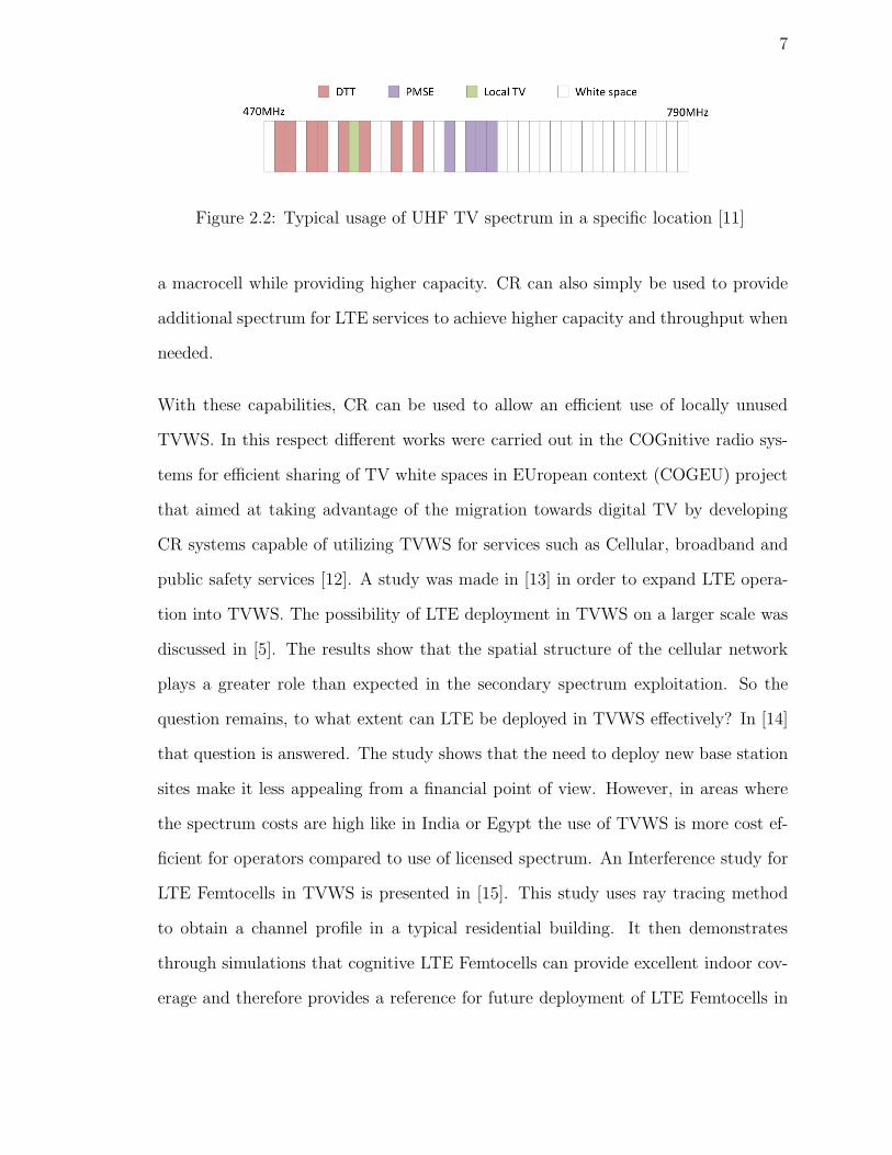
The United States and Europe respectively. Fig.2.2 shows how underutilized is the

TV band in a specific location in the UK with less than 50% utilization. Tremendous

effort was put into researching possible ways to salvage and reuse this WS to aid in

the support of other services such as Long term Evolution (LTE) as seen in [4–7].

To put some of these strategies and studies into action, there is a noticeable focus

on specific technologies in the wireless communications research area to facilitate

that. One of such technologies is Cognitive Radio (CR). CR technology was initially

proposed by Joseph Mitola in [8] as a concept of a radio capable of adapting and

learning from the environment. This capability has proven useful in the area of

spectrum sharing and has been used ever since to resolve the problem of increasing

spectrum requirements in a world where very scarce spectrum resources exist.

5

6

Figure 2.1: IMT spectrum requirements forecast [9]

CR technology enables Secondary Users (SU), LTE in our case, to monitor the spec-

trum regularly and even use it in idle periods. Once the Primary User (PU) needs

the channel again, the SU switches to a different channel or terminate the commu-

nication sequence to avoid interfering with the PU. The idea here is that SUs have

to be completely transparent to the PU. Meaning that the PU functions in normal

operation mode without being altered or modified by the existence of a SU. Concepts

such as spectrum management and spectrum sharing are explained in more details

in [10].

There are many applications for CR technology. Fig.2.3 shows some operational

scenarios for CR. It can be used to provide LTE over TVWS in rural or indoor areas

by transmitting below a certain transmit power threshold. CR can also use TVWS for

backhaul communications with the LTE core network. Using CR technology, small

cells can use TVWS to avoid the co-channel interference among nearby small cells or

7

Figure 2.2: Typical usage of UHF TV spectrum in a specific location [11]

a macrocell while providing higher capacity. CR can also simply be used to provide

additional spectrum for LTE services to achieve higher capacity and throughput when

needed.

With these capabilities, CR can be used to allow an efficient use of locally unused

TVWS. In this respect different works were carried out in the COGnitive radio sys-

tems for efficient sharing of TV white spaces in EUropean context (COGEU) project

that aimed at taking advantage of the migration towards digital TV by developing

CR systems capable of utilizing TVWS for services such as Cellular, broadband and

public safety services [12]. A study was made in [13] in order to expand LTE opera-

tion into TVWS. The possibility of LTE deployment in TVWS on a larger scale was

discussed in [5]. The results show that the spatial structure of the cellular network

plays a greater role than expected in the secondary spectrum exploitation. So the

question remains, to what extent can LTE be deployed in TVWS effectively? In [14]

that question is answered. The study shows that the need to deploy new base station

sites make it less appealing from a financial point of view. However, in areas where

the spectrum costs are high like in India or Egypt the use of TVWS is more cost ef-

ficient for operators compared to use of licensed spectrum. An Interference study for

LTE Femtocells in TVWS is presented in [15]. This study uses ray tracing method

to obtain a channel profile in a typical residential building. It then demonstrates

through simulations that cognitive LTE Femtocells can provide excellent indoor cov-

erage and therefore provides a reference for future deployment of LTE Femtocells in

8

Figure 2.3: Different scenarios of CR in LTE networks [9]

TVWS. In [4, 16] a smaller scenario was considered. The study proved that indoor

LTE small cells operation is possible and feasible in the Adjacent Channel (AC) to

that of Digital TV. Despite proven feasible and cost efficient, almost non of the pre-

vious works in this area discussed the process of deploying LTE small cells in TVWS.

That is why in this thesis will complement previous works by devising a systematic

approach to deploying indoor LTE small cells in TVWS.

2.2 Indoor Network Planing

2.2.1 Introduction

Planning and optimization of cellular network resources constitutes one of the funda-

mental components in network design. An efficient network design through intelligent

planning and optimization could have significant impacts on networks cost while in-

creasing their supported capacities. Indoor planning and optimization in particular

is of ultimate essence since it is safe to assume that the bulk of broadband traffic is

9

generated indoors. In fact, the importance of indoor planning has only become evi-

dent after the introduction of Distributed Antenna Systems (DAS) to enhance indoor

coverage. In DAS, multiple antennas are used to provide coverage within a building.

This guarentees a better chance for Line of Sight (LOS) situations with the prospect of

improving the received signal quality.Accordingly, clever planning and optimization in

DAS invokes designing the antenna layout (i.e., number/locations of antennas as well

as the corresponding feeding network) with the prospect of maximizing throughput

capacity.Previously, it usually took the efforts and experience of engineers to manually

manage the network planning and optimization process through site survey.

As an effective means to improve indoor broadband services, small cells has become a

research focus. Unlike DAS, small cells are designed with full base station capabilities

(i.e., Frequency reuse, Handover, etc.) reducing the need for backhaul communica-

tions over radio link. Besides being low cost and low power, it can provide high

quality, high speed broadband services with coverage areas raging from small rooms

to big halls. They not only extend the Macro-cell coverage area for indoor scenarios

but they also can achieve higher data rates. However, since the distances between the

small cells are short, the interference is relatively strong. As a result, the optimization

requirements for indoor small cell scenarios are much more complicated than those

of outdoor environments.

2.2.2 Indoor Planning for Small Cells

Over the past few years there has been a significant number of tools developed for

indoor small cells planning and optimization based on analytical and numerical ap-

proaches. While analytical approaches are simpler and faster than numerical ap-

proaches, they imply a great deal of complex analysis when an optimization has to

10

Figure 2.4: Scenario Plan in 2D and 3D [15]

be performed. One of many popular approaches is using the simplex optimization

algorithm to optimally place transmitters in a given floor. In [17] a transmitter place-

ment method is presented based on a hierarchical simplex search algorithm. Using this

approach near optimal transmitter placement is guaranteed. However, like many oth-

ers, this algorithm only optimizes the number and locations of transmitters, lacking

therefore the ability to optimize transmit powers of previously placed transmitters.

As most of indoor planning tools, this algorithm considers every floor separately dur-

ing the optimization process. As seen in Fig.2.4 floor plans are used in the simulation

and not entire building plans, which in turn results in a significant loss of resources

since a user can receive coverage from another floor with more efficient planning

measures.

Indoor planning and optimization, as explained before, is a multi-objective optimiza-

tion problem. One way of solving multi-objective optimization problems is using

Genetic Algorithms (GA). A genetic algorithm starts with a population of all fea-

sible locations. A one dimensional objective function is then used as an indicator

of the fitness of every individual in the population. Multiple individuals are then

11

stochastically selected based on their fitness to form the new population. When the

algorithm terminates due to maximum number of iterations it theoretically does not

guarantee optimum solutions. A solution for indoor coverage optimization with GAs

is presented in [18, 19].

In [20] a comparative study between two different optimization techniques (Krig-

ing and GA) for optimal transmitter location in indoor environments is presented.

This study showed that Kriging is an efficient tool for solving indoor optimization

problems limited to the position of a single transmitter. This approach was indeed

later extended for several transmitters in [21] using Transmission Line Matrix (TLM).

TLM is a well-established method for wave propagation simulation. The advantage

TLM presents is that it takes into account all the interactions between waves and

furniture, structures and building plan. Due to the complexity of the transmitter’s

environment, TLM is first used to provide an accurate propagation model of the chan-

nel. This model makes it clear where it would be most beneficial to add a secondary

transmitter. The combination of Kriging and TLM provides an automatic planning

tool for the optimization of multiple transmitter locations in indoor environments.

A more advanced adaptive indoor optimization algorithm is presented in [22]. The

Adaptive Distributed Femtocell Coverage Optimization (ADFCO) algorithm is used

in LTE indoor enterprise environments. The ADFCO algorithm updates the trans-

mitter power of femtocells depending on the users. Therefore, reducing unwanted

handovers and decreases coverage gaps and overlaps. Numerical results shows 50%

enhancement of overall capacity when compared to fixed transmitter power allocation

techniques. Being the opposite of the previous algorithms, the ADFCO optimizes the

power of transmitters but it has no way of optimizing the locations of the transmitters

which has to be done manually through network planning experience.

12

While some of these works are very efficient in solving the indoor optimization problem

in normal and even challenging indoor environments, none has considered utilizing

the TVWS. Motivated by the lack of studies focusing on indoor planning considering

TVWS requirements, in this paper, we propose a systematic approach to deploy LTE

small cells in indoor environments while utilizing TVWS to support LTE services.

This approach is an automatic tool that solves a very complex multi-objective op-

timization problem combining locations, powers and number of transmitters. This

aids in the lowering of the traffic load on the Macro-cells and provides higher data

rates indoors. This algorithm is very mathematically simple yet it delivers promising

results and opens the door for more research not only focusing on LTE planning but

also on general indoor network planning utilizing TVWS. Moreover, This approach

considers the building plan as a whole, therefore, using resources more efficiently than

other algorithms that work on a floor-by-floor basis. This not only lowers power ex-

penditure, but results as well in less interference which in turn helps maintain high

SINR values leading to an increase in overall capacity.

Chapter 3

Methodology

3.1 Assumptions

3.1.1 Scenario

Measurements of the DVB-T signals were comprehensively collected in [16] for the

building of the department of Signal Theory and Communications (D4) in Universitat

Politecnica de Catalunya · BarcelonaTech (UPC) Campus Nord (latitude: 41°23’

20” N; longitude: 2°6’ 43” E; altitude: 175 m). Therefore, the indoor environment

was chosen to be the same building. The Position of the DVB-T transmitter and

location of considered building are shown in Fig.3.1. The building consists of 3 floors

and 1 basement floor. Indoor measurements of DVB-T signal for channels 26 (514

MHz), 44(658 MHz) and 61(794 MHz) were performed in the study presented in [16].

Conclusions of this study states that it is indeed feasible to construct such a map that

will allow for reliable deployment of new secondary transceivers within the building

and for coexistence of different systems.

As a reference for the evaluation 83 measurement points were defined within the entire

building as shown in Fig.3.5. Measurements used in this work correspond to channel

61 (794 MHz). For the scope of this thesis we will consider the worst case scenario,

where the positions of the DVB-T receivers are unknown. We assume that DVB-T

receivers can be located at any of these points via portable USB receivers connected

13

14

to laptops. However, in other scenarios it can also be considered where the positions

of the DVB-T receivers are static or in which the only DVB-T reception point is the

antenna on the rooftop. For the sake of simplicity, only these measurement points

will be used. However, the same methodologies can be applied if more points exist or

if interpolation is used to define more measurement points, but this is left for future

works.

The locations of the measurement points are shown in Fig.3.3. These locations will

be referenced many times throughout the text by their index number. For example,

position 83 represents the measurement point located at D4-111-B (X = 29 m, Y =

13 m, Z = 7.5 m).

Figure 3.1: Position of DVB-T tower and measured building [4]

15

Figure 3.2: First floor measurement points in the building and the coordinate axis [4]

3.1.2 Radio Environment Map Information

The concept of Radio Environment Maps (REM) was first introduced by Virginia

Tech scholars in [23]. REMs are centralized or distributed databases containing multi-

dimensional cognitive information on the radio environment such as device locations

and their activities, policies and regulations, etc. The main functionality of REMS is

storage of Geo-localized measurements. The use of REMs reduces the requirement for

measurements and allows for more dynamic processing of data stored such as spatial

or temporal interpolation of measurements. A successful Radio Environment Map

should include all information needed for deploying secondary transmitters (small

cells) in the indoor environment where it applies to.

The REM database from previous works [4,16], on which this approach is based, was

16

Figure 3.3: Measurement points located inside the building with their coordinates inmeter, office location and index. Index is used to reference different points throughoutthis thesis

17

generated and stored using Microsoft Excel sheets. While being conveniently sim-

ple, it lacked the functionality needed to tackle complex multi-objective optimization

problems which require rigorous simulations and a high level of automation. There-

fore, it was essential to integrate this data using a tool such as Matlab. Some of this

data is:

� R(θ, θ′): Separation in meters between any two points of the building. Where

the coordinates for one position are denoted as θ = (x, y, z)

� L(R, n): Indoor propagation model to characterise the losses between any two

points of the building as a function of the separation R and building character-

istics (e.g. number of floors, etc.).

� Pr(θ,N): Received power level of the DVB-T signal at each position θ inside

the building .

A 3D plot of the measurement points inside our building is shown in Fig.3.4. This

was possible to produce after loading all the data needed from the Excel sheets into

matlab. Other needed data was generated using mathematical models that will be

explained later on. Having all the required data in Matlab makes it possible to

perform complex simulations and use more advanced optimization algorithms.

Now we turn our attention to some of our REM’s content. This REM describes some

of the parameters in our scenarios such as power limitations, interference and indoor

propagation model. We will discuss each of these parameters in the following sections.

18

3025

2015

105

00

2

4

6

8

10

12

7

6

8

2

5

4

3

1

014

Figure 3.4: 3D plot of the measurement points inside our building

Protection Ratio (PR)

One of the important pieces of information in our REM is the power limitation that

results from the condition that the interference generated by secondary transmitters

to any DVB-T receiver should be below a certain threshold not to degrade the TV

reception. Requirements for successful DVB-T reception have been defined in lit-

erature [24–26]. These requirements are usually expressed in terms of the so-called

Protection Ratio (PR). PR is defined as the minimum required ratio between the

DVB-T signal received and the interference at a certain point, meaning that it should

be satisfied that

PR

I≥ PR (3.1)

Where PR is the received DVB-T signal and I is the total interference. It is important

to note that PR depends on several factors. For instance, whether the DVB-T signal

and the secondary transmitter are operating in the same channel and thus generate

co-channel interference or in adjacent channels. In the case of adjacent channels the

PR depends strongly on the selectivity of the DVB-T receiver and on the Adjacent

19

Figure 3.5: First floor measurement points in the building [4]

Channel Leakage Ratio (ACLR) of the secondary transmitter (being LTE in our case)

which determines how much power exactly are leaked to adjacent channels. For the

scope of this work we take as a reference a fixed PR value of -31 dB. This value

was determined based on extensive measurements done in [26] for different types of

DVB-T receivers and LTE transmitters while assuming LTE transmission in the first

adjacent channel. This value, for the sake of future work, can be adjusted depending

on the type of hardware used and in no way limits the operation of this approach.

One more thing that has to be taken into consideration is that results obtained

in [4] reveal that in the considered building small cell deployment using co-channel

transmission is not feasible due to the very low resulting allowed transmit power.

Therefore, we limit our investigation in this paper to adjacent channel transmission,

which was found more adequate for successful small cells deployment.

20

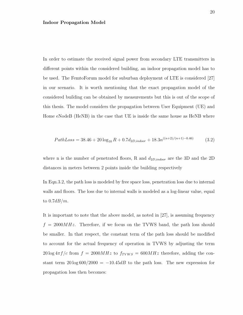
Indoor Propagation Model

In order to estimate the received signal power from secondary LTE transmitters in

different points within the considered building, an indoor propagation model has to

be used. The FemtoForum model for suburban deployment of LTE is considered [27]

in our scenario. It is worth mentioning that the exact propagation model of the

considered building can be obtained by measurements but this is out of the scope of

this thesis. The model considers the propagation between User Equipment (UE) and

Home eNodeB (HeNB) in the case that UE is inside the same house as HeNB where

PathLoss = 38.46 + 20 log10R + 0.7d2D,indoor + 18.3n((n+2)/(n+1)−0.46) (3.2)

where n is the number of penetrated floors, R and d2D,indoor are the 3D and the 2D

distances in meters between 2 points inside the building respectively

In Eqn.3.2, the path loss is modeled by free space loss, penetration loss due to internal

walls and floors. The loss due to internal walls is modeled as a log-linear value, equal

to 0.7dB/m.

It is important to note that the above model, as noted in [27], is assuming frequency

f = 2000MHz. Therefore, if we focus on the TVWS band, the path loss should

be smaller. In that respect, the constant term of the path loss should be modified

to account for the actual frequency of operation in TVWS by adjusting the term

20 log 4πf/c from f = 2000MHz to fTVWS = 600MHz therefore, adding the con-

stant term 20 log 600/2000 = −10.45dB to the path loss. The new expression for

propagation loss then becomes:

21

PathLoss = 28.01 + 20 log10R + 0.7d2D,indoor + 18.3n((n+2)/(n+1)−0.46) (3.3)

3.2 Approach 1: Maximizing Total Transmitted Power

3.2.1 Optimization Problem Introduced

In order to formulate our general optimization problem we have to start at the base

of our scenario and work our way through different assumptions until we reach a solid

general statement that describes our problem comprehensively.

1. Maximum allowed transmit power when there is no other secondary transmitters

in the building

Assuming there is no other secondary transmitter in the building, the maximum

allowed transmit power at any point θ = (x, y, z) for an adjacent channel N + i

has to fulfill the following condition for any point θ′ where a DVB-T receiver

might be located:

Pr(θ′, N)

PTmax(θ,N + i)/L(θ′, θ)

≥ PR(i) (3.4)

where L(θ, θ′) is the path loss between point θ where the secondary transmitter

is located and point θ′ where a DVB-T receiver might be located, and i denotes

the number of adjacent channel considered for operation. Fulfilling the condition

3.4 requires that the following expression be minimized:

22

PTmax(θ,N + i) = min

θ′ s.t. Pr(θ′,N)≥Prmin

[

Pr(θ′, N) · L(θ′, θ)

PR(i)

]

(3.5)

For the case θ = θ′ which suggests that the secondary transmitter and the

DVB-T receiver are located in the same position, we assume that minimum

physical separation will always exist between the two [28], so L(θ′, θ) equals

a minimum propagation loss Lmin which depends on the physical separation.

Typical values for PR(i) are low enough in the case of adjacent channel N + i

that even allow secondary transmission at a point where DVB-T reception in

channel N is possible.

2. Maximum allowed transmit power when there is another secondary transmitter

placed in the building

Now assuming there is another secondary transmitter already deployed at posi-

tion θ∗ with transmit power PTsec, then the maximum transmit power allowed for

a new secondary transmitter located at position θ, following the same approach

as before, will be:

PTmax(θ,N + i) = min

θ′ s.t. Pr(θ′,N)≥Prmin

[

L(θ, θ′)(Pr(θ

′, N)

PR(i)−

PTsec(θ∗, N + i)

L(θ∗, θ′)

)

]

(3.6)

However, the transmit power computed above assumes that when the second

secondary transmitter is deployed, the first secondary transmitter is not modi-

fied in any way. This does not guarantee maximum total transmit power. For

that, we would need to jointly determine the maximum allowed power of both

23

secondary transmitters simultaneously, or equivalently, at the time of deploy-

ment of the second transmitter, we will have to recompute the power of both

transmitters.

3. Maximum allowed transmit power when there are multiple secondary transmit-

ters placed inside the building

Knowing now that transmit powers should be jointly optimized simultaneously,

we would like to determine the maximum allowed power of each of K secondary

transmitters located at positions θk=1,2,..K so that the aggregated interference

generated onto a DVB-T receiver located at any position θ′ is acceptable. Equiv-

alently, the following condition must hold at any point θ′ where a DVB-T re-

ceiver might be located:

Pr(θ′, N)

K∑

k=1

PTk(θk,N+i)

L(θ′,θk)

≥ PR(i) ∀θ′ s.t. Pr(θ′, N) ≥ Prmin

(3.7)

The general multi-objective optimization problem can be then defined as follows:

maxPTk

,θk(PT1

, PT2, ..., PTK

)

s.t.Pr(θ

′, N)K∑

k=1

PTk(θk ,N+i)

L(θ′,θk)

≥ PR(i) ∀θ′ s.t. Pr(θ′, N) ≥ Prmin

(3.8)

Where we have to find the positions and transmit powers of secondary transmitters

that maximizes the secondary transmit power inside the building.

24

3.2.2 Proposed Algorithm

There are many techniques to handle multi-objective optimization problems as the

one we have on hand. One possibility is to convert the multi-objective optimization

to a single objective optimization by combining the different optimization objectives

(i.e. secondary transmit powers in our case). In this respect, a viable solution is to

consider the aggregate transmit power of secondary transmitters. In this case, our

optimization problem becomes:

maxPTk,θk

(PT1 + PT2 + ...+ PTK)

s.t.Pr(θ

′, N)K∑

k=1

PTk(θk ,N+i)

L(θ′,θk)

≥ PR(i) ∀θ′ s.t. Pr(θ′, N) ≥ Prmin

(3.9)

Now with Eq.3.9 we have a much simpler optimization problem than the multi-

objective Eq.3.8. To solve this problem, we adapt the sectioning method, a direct

search algorithm, to our need [29]. Our approach works as a direct search method.

First of all, initial positions and powers are assigned to K-1 secondary transmitters.

It starts by calculating the maximum possible transmit power of the Kth secondary

transmitter, taking into consideration the other K-1 secondary transmitters, by solv-

ing Eqn.3.9 using initial values for the first iteration. Then in a recursive manner,

it keeps calculating maximum possible transmit powers until a maximum is reached.

Convergence happens when the powers and positions of secondary transmitters stop

changing, which occurs after a few iterations. The general flow chart of our algorithm

is shown in Fig.3.6.

There are 2 different variables being optimized in Eq. 3.9. Transmit power PTk and

25

Figure 3.6: Flow chart of the recursive algorithm used in our first approach

26

location θk. As can be seen in Fig.3.6, there are multiple loops performing different

operations. First of all, choosing the initial point is very important as it affects the

accuracy of the results as will be demonstrated in the results section. The innermost

loop (1) computes the maximum transmit power for a secondary transmitter placed

at any of the measurement points. This is done by calculating the maximum transmit

power at each measurement point, denoted by its index i (representing possible θk),

while still satisfying Eq. 3.7 at any DVB-T receiver position, denoted by its index

j (representing θ′). Then, the minimum of all these possible transmitter powers is

chosen in (2) because it is the transmit power that satisfies Eq. 3.7 for all positions

j (θ′). After that, the outer loop (3) changes the transmitter position i, and repeats

both operations (1) and (2) until all measurements points are checked. It then chooses

the position with maximum secondary transmit power, and by doing that optimizes

the position as well as the power. Finally, the algorithm does multiple iterations of

the previous steps, iterating from one transmitter to another, until they all converge.

Operation (4) considers only the last K iterations representing the number of trans-

mitters considered. Since each iteration represents the optimization process of one

secondary transmitter, then results of these last K iterations represent optimum posi-

tions and powers of all K secondary transmitters. The algorithm returns the optimum

power and location of secondary transmitters for indoor deployment. The algorithm

in Fig.3.6 is for a fixed number of transmitters K. Repeating this for different numbers

of transmitters K allows us to examine the effect of K on total secondary transmit

power.

While the number of secondary transmitters deployed inside the building K is present

in the optimization problem, it has no sense to make it an optimization objective as an

increase in the number of secondary transmitters will always constitute an increase

in total secondary transmit power. Also, as will be discussed in more details in

27

Figure 3.7: Illustration of how the algorithm works

the results section, while an increase in the number of secondary transmitters most

definitely constitutes an increase in total transmit power, it is not always considered

beneficial from a network throughput or capacity point of view.

To better describe the details of our approach, let us consider the case of only two

secondary transmitters placed at arbitrary locations and take a look at how the

algorithm operates. The basic idea of a direct search algorithm is that it operates

on each axis (corresponding to one secondary transmitter in our case) separately as

illustrated in Fig.3.7. The algorithm starts by maximizing the transmit power for the

first transmitter, then maximizes the transmit power for the second transmitter and

keeps doing that recursively until a maximum is reached.

28

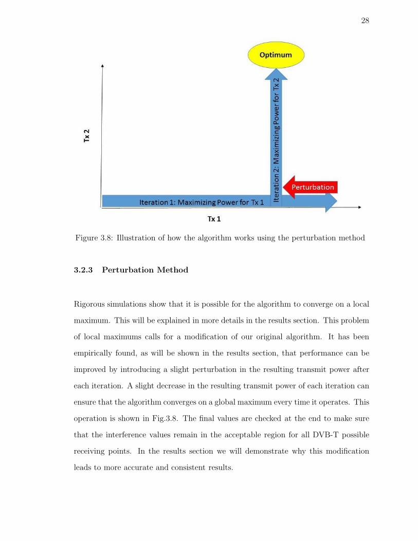
Figure 3.8: Illustration of how the algorithm works using the perturbation method

3.2.3 Perturbation Method

Rigorous simulations show that it is possible for the algorithm to converge on a local

maximum. This will be explained in more details in the results section. This problem

of local maximums calls for a modification of our original algorithm. It has been

empirically found, as will be shown in the results section, that performance can be

improved by introducing a slight perturbation in the resulting transmit power after

each iteration. A slight decrease in the resulting transmit power of each iteration can

ensure that the algorithm converges on a global maximum every time it operates. This

operation is shown in Fig.3.8. The final values are checked at the end to make sure

that the interference values remain in the acceptable region for all DVB-T possible

receiving points. In the results section we will demonstrate why this modification

leads to more accurate and consistent results.

29

As shown in the Figure, the subtraction of the perturbation value causes the optimiza-

tion algorithm to steer the result away from any local maximums that can produce

wrong results. Empirical trial and error experiments were performed to decide an

optimal value for the perturbation. It was found that best results, which mean guar-

anteed convergence, occur at a value of 0.2 dB. This value is subtracted from the

resulting power of each iteration in dBm. Lower values of the perturbation do not

provide a solution for the problem of inconsistency, while higher values of the pertur-

bation cause deviation from the global optimum which increases with the increase of

this value.

3.3 Approach 2: Optimizing Performance Based on SINR

3.3.1 Optimization Problem Introduced

An increase in the number or power of secondary transmitters means an increase in

Inter Cell Interference (ICI) which in turn, decreases the Signal to Interference and

Noise Ratio (SINR) and capacity of the network. Therefore, a second approach is

suggested. Our general optimization problem so far was formulated based on maxi-

mizing transmit power of secondary transmitters. However, this leads to a decrease in

the average SINR in the building leading to lower capacity values as will be explained

in details in the results section. Therefore, this is not the most efficient approach.

For that, we have to formulate a new optimization problem that takes more into

consideration network throughput and capacity. We first define a QI representing the

percentage of positions in the building above a desired SINR threshold. Then, our

second approach is to maximize this QI while keeping the interference levels in all

DVB-T possible receiving positions within the acceptable range. Our new optimiza-

tion problem is then:

30

arg maxPTk,θk,K

(QI)

s.t.Pr(θ

′, N)K∑

k=1

PTk(θk ,N+i)

L(θ′,θk)

≥ PR(i) ∀θ′ s.t. Pr(θ′, N) ≥ Prmin

(3.10)

Where QI is the percentage of positions θ′ where the following condition holds:

PTn(θn)/L(θ′, θn)

PNoise +K∑

k=1k 6=n

PTk(θk,N+i)

L(θ′,θk)

≥ SINRth (3.11)

Where Transmitter n is the transmitter providing coverage to position θ′ (i.e. the

transmitter with highest received power PTn/L(θ′, θn) , SINRth is the desired SINR

based on modulation and encoding requirements, and the noise power measured in

the channel is:

PNoise = K · to · F · B (3.12)

Where B = 8MHz and K · to = −174 dBm/Hz, and Noise Figure (F) is assumed to

be 7 dB. The noise power is then PNoise ≃ −98 dBm.

From what can be seen in Eqn.3.11, and unlike our first approach, the number of

transmitters K is an important objective in our optimization problem. This opti-

mization problem tries to maximize the introduced QI by optimizing three different

31

variables. The number of secondary transmitters K, the transmit power of each sec-

ondary transmitter PTkand the location of each secondary transmitter θk. It is also

important to note that the expression in Eqn.3.11 does not consider the interference

generated by DVB-T transmitters operating in the adjacent channel. This will be

explained in more detail in the next section.

3.3.2 Interference Generated by DVB-T Transmitters

The interference exerted from DVB-T transmitters on LTE receivers must be consid-

ered for successful LTE operations. This interference can handicap the LTE service

operations, therefore has to be monitored and mitigated. It depends on the selectivity

of LTE receivers and the ACLR of DVB-T transmitters. According to the following

expression, where PRx is the power received by DVB-T receivers in the adjacent

channel:

I = PRx(1

Selectivity+

1

ACLR) (3.13)

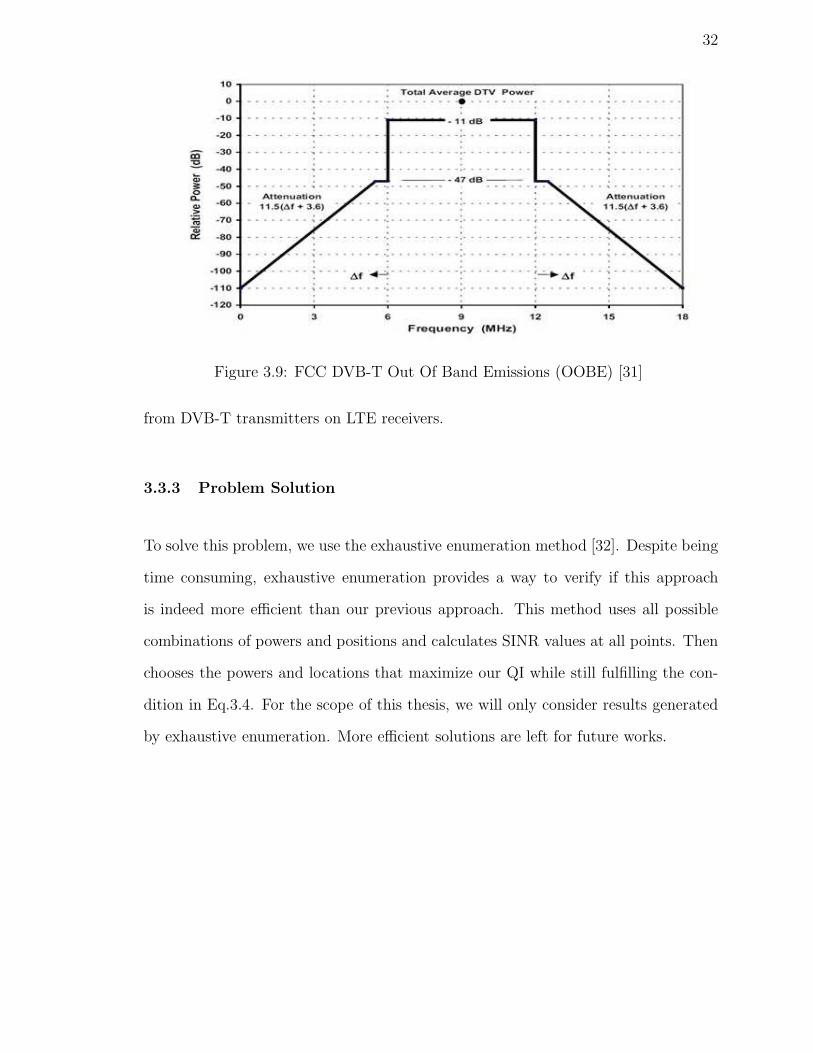
In [30] the selectivity of LTE receivers are found to be in the range of 43 dB. In [31]

the ACLR of DVB-T transmitters as shown in Fig.3.9 are found to be 55 dB for

adjacent channels N ± 1. Moreover, the average DVB-T PRx was found in [16] to

be ranging from -58 dBm to -78 dBm depending on the position within our indoor

environment. in this respect, the interference values are in the range of -100 dBm to

-120 dBm, which is lower than the noise power (PNoise = −98dBm). These values are

also relatively low when compared to ICI between different small cells (i.e. different

secondary transmitters) which our simulations show that it ranges between -80 dBm

and -100 dBm. Therefore, in our study, it is safe to neglect the interference exerted

32

Figure 3.9: FCC DVB-T Out Of Band Emissions (OOBE) [31]

from DVB-T transmitters on LTE receivers.

3.3.3 Problem Solution

To solve this problem, we use the exhaustive enumeration method [32]. Despite being

time consuming, exhaustive enumeration provides a way to verify if this approach

is indeed more efficient than our previous approach. This method uses all possible

combinations of powers and positions and calculates SINR values at all points. Then

chooses the powers and locations that maximize our QI while still fulfilling the con-

dition in Eq.3.4. For the scope of this thesis, we will only consider results generated

by exhaustive enumeration. More efficient solutions are left for future works.

Chapter 4

Results

After introducing our approaches, it is important to see how they perform in our

scenario. Several simulations have been executed to test our algorithms in many

aspects such as accuracy, time consumption and network throughput.

4.1 Approach 1 Results

4.1.1 Original Algorithm

The proposed algorithm returns the position (represented by the index of the mea-

surement point corresponding to it) and transmit power of secondary transmitters

to achieve maximum possible total secondary transmit power. Using exhaustive

search [32], it was possible to examine the effect of changing the initial point on

the recursive algorithm. The algorithm is calculated 83 times with 83 different initial

points with the same initial power. Results shown in Fig.4.1. These simulations show

that results vary depending on the initial points used. Different locations and powers

appear every time the initial point is changed which leads to inconsistent (changing

with changing of initial point) and possibly unreliable (optimum is not guaranteed)

algorithm output.

In order to analyze the source of this behavior, the power profile of two transmitters

placed at positions D4-005-B and D4-111-B is depicted in Fig.4.2. Using all possible

33

34

Figure 4.1: Results of the proposed algorithm with K = 2 for different initial points.Column 1: initial position used in the algorithm, column 2,3: optimal transmitterpositions for transmitter 1 and 2 for maximum total transmit power, columns 4,5:maximum transmit power for transmitter 1 and 2 in dBm, columns 6: total transmitpower from both transmitters in dBm.

transmit power combinations, the interference at all possible DVB-T receivers is cal-

culated. Power combinations that satisfy the interference constraints in Eq. 3.7 are

then plotted in green, and power combinations that do not fulfill these constraints

are plotted in red. As you can see the power profile is very linear, except for the

marked area. This marked edge is considered a local maximum. Applying the basic

concept of operation explained in Fig.3.7 then it is possible to converge onto this local

maximum as indicated on Fig.4.2.

4.1.2 Perturbation Method

Considering Two secondary transmitters K=2

This method was introduced to the original algorithm in order to provide a solution

for the above-mentioned problem of local maximums. To determine a suitable value

35

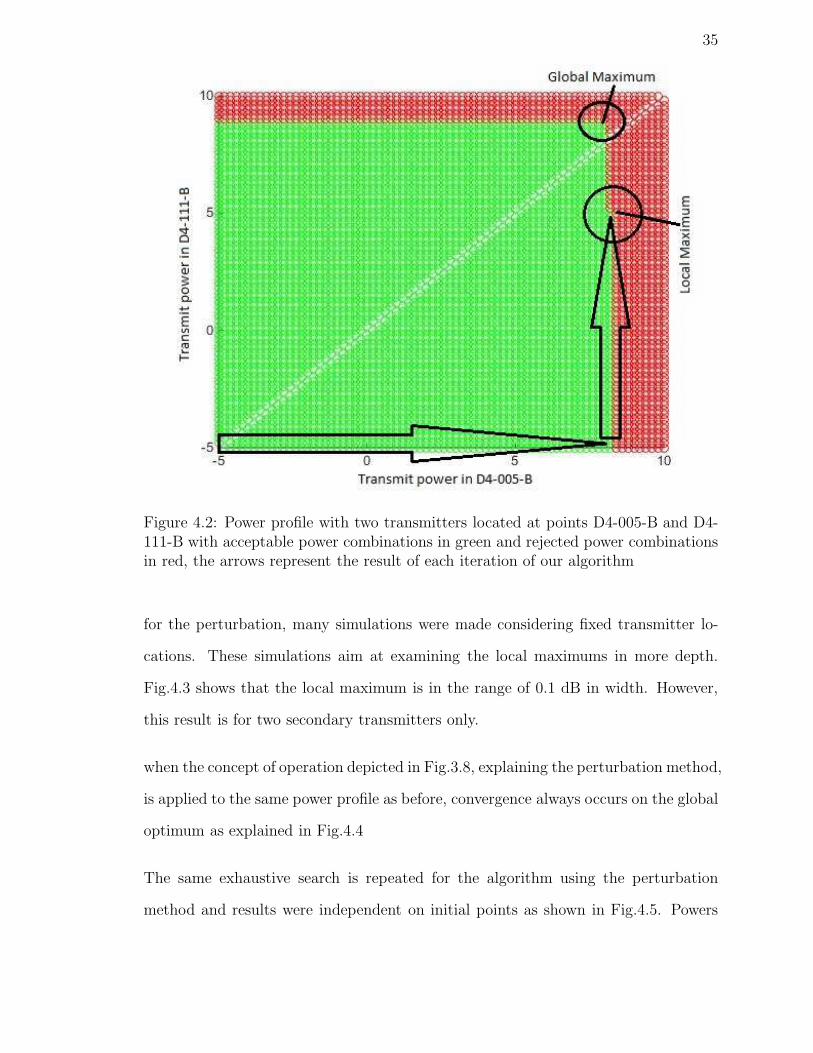
Figure 4.2: Power profile with two transmitters located at points D4-005-B and D4-111-B with acceptable power combinations in green and rejected power combinationsin red, the arrows represent the result of each iteration of our algorithm

for the perturbation, many simulations were made considering fixed transmitter lo-

cations. These simulations aim at examining the local maximums in more depth.

Fig.4.3 shows that the local maximum is in the range of 0.1 dB in width. However,

this result is for two secondary transmitters only.

when the concept of operation depicted in Fig.3.8, explaining the perturbation method,

is applied to the same power profile as before, convergence always occurs on the global

optimum as explained in Fig.4.4

The same exhaustive search is repeated for the algorithm using the perturbation

method and results were independent on initial points as shown in Fig.4.5. Powers

36

Figure 4.3: Power profile with two transmitters located at points D4-005-B and D4-111-B with acceptable power combinations in green and rejected power combinationsin red, the values shown represent the width of the local maximum valley

Figure 4.4: Power profile with two transmitters located at points D4-005-B and D4-111-B with acceptable power combinations in green and rejected power combinationsin red, the arrows represent the result of each iteration of our algorithm

37

Figure 4.5: Results of exhaustive search to examine the effects of changing the initialpoint on the performance of the algorithm using the perturbation method

shown in previous Fig.4.1 appear to be in some cases higher than the optimum re-

sulting in Fig.4.5. This is expected as the algorithm reaches an answer as close as

possible to an optimum in the order of 0.1 dB as shown by the difference between the

highest power value in Fig.4.1 which is 11.576 dBm and the power values shown in

Fig.4.5 of 11.473 dBm. This is a small sacrifice in order to make the algorithm more

consistent.

Fig.4.6 shows graphically the optimum locations and transmit powers for the case

of 2 transmitters. as you can see the algorithm shows the locations and gives the

transmit power in dBm.

Considering Three Secondary Transmitters K=3

Further analysis was performed using higher number of transmitters and values of

perturbations varying around 0.1 dB. Due to dimensionality problems, it is difficult

to show it graphically. However,Fig.4.7 and Fig.4.8 show results of the algorithm

using the perturbation method for 3 secondary transmitters with perturbation values

38

Figure 4.6: Location and powers of optimum secondary transmitters with limit ofonly 2 transmitters

of 0.1 dB and 0.2 dB respectively and different initial points. These simulations

proved, as mentioned in section 3.2.3, that higher values than 0.2 dB of perturbation

causes a much higher deviation from the optimum transmit power value, and lower

values than 0.1 dB produces very inconsistent results.

Fig.4.9 shows graphically the optimum locations and transmit powers for the case

of 3 transmitters. as you can see the algorithm shows the locations and gives the

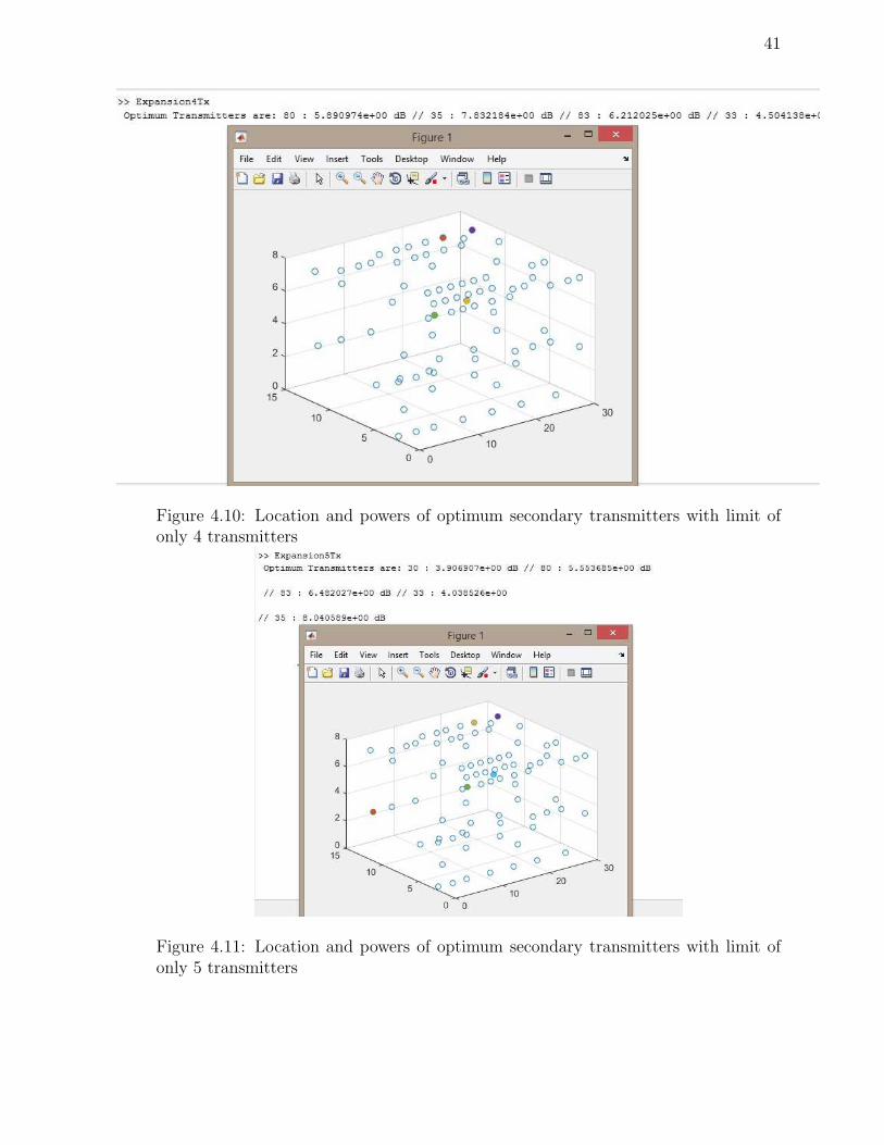
transmit power in dBm. The results for 4 and 5 transmitters are shown in Fig.4.10 and

Fig.4.11. We observe that the transmitters are always clustered in one area (first floor,

North side). This observation is explainable if we consider the location of the DVB-T

transmitter. In order to provide higher secondary transmit power, the algorithm had

to place the transmitters in positions with higher DVB-T received signal strength,

that are closest to the DVB-T transmitter located north of the building, so that the

PR constraint in Eq.3.7 stays fulfilled while increasing secondary transmit power.

39

Figure 4.7: Results of the proposed algorithm with K = 3 for different initial pointsand 0.1 dB perturbation. Columns 1: initial position used in the algorithm, columns2,4,6: optimal transmitter positions for transmitter 1, 2 and 3 for maximum totaltransmit power, columns 3,5,7: maximum transmit power for transmitter 1, 2 and 3in dBm, column 8: total transmit power in dBm.

Figure 4.8: Results of the proposed algorithm with K = 3 for different initial pointsand 0.2 dB perturbation. Column 1: initial position used in the algorithm, columns2,4,6: optimal transmitter positions for transmitter 1, 2 and 3 for maximum totaltransmit power, columns 3,5,7: maximum transmit power for transmitter 1, 2 and 3in dBm, column 8: total transmit power in dBm.

40

Figure 4.9: Location and powers of optimum secondary transmitters with limit ofonly 3 transmitters

4.1.3 Effect of the approach on average SINR

In order to investigate the efficiency of our approach from a SINR point of view, total

transmit power is plotted on the same curve as the average SINR against the increas-

ing number of secondary transmitters for the cases of 2, 3, 4, and 5 transmitters.

Results are shown in Fig.4.12. As can be seen, increasing the number of transmitters

causes an increase in total transmit power. This, in turn, causes an increase in ICI

and results in a drop in the average SINR (defined as the averaging of measured

SINR between all measurement points). This drop is also emphasized by the cluster-

ing of secondary transmitters. In the case of 5 transmitters, a secondary transmitter

is placed in the other side of the building away from the transmitter cluster. This

positioning causes the average SINR to be higher than in the case of 4 transmitters.

With these results, it is very clear that maximizing total secondary transmit power

41

Figure 4.10: Location and powers of optimum secondary transmitters with limit ofonly 4 transmitters

Figure 4.11: Location and powers of optimum secondary transmitters with limit ofonly 5 transmitters

42

Figure 4.12: A graph showing how total transmit power and SINR change withincreasing number of transmitters

is not the most efficient approach from a SINR perspective or equivalently from a

capacity perspective.

4.1.4 Exhaustive Enumeration

The method of Exhaustive enumeration (brute force) was chosen to be compared

with our suggested algorithms. It is a simple discrete optimization technique. It first

evaluates the optimum solution for all combinations of the discrete variables, then

the best solution is obtained by scanning all the optimum solutions. It is a very time

consuming algorithm. The time consumption depends greatly on the resolution of

the discrete variables. It is important to note that if the resolution of the discrete

variables was to tend to zero, exhaustive enumeration would provide exact results of

the optimum. However, this can not be done since the time needed will tend, in this

case, to infinity.

43

Figure 4.13: Results of exhaustive enumeration (brute force) method

Before using the different proposed approaches in simulations, it was crucial to have a

benchmark that guides the evaluation process. Results of the exhaustive enumeration

method is shown in Fig.4.13.

When comparing our approach to exhaustive enumeration, the power values provided

by our algorithm are very accurate. While exhaustive enumeration results in a total

secondary transmit power of 11.2675 dBm with very high time consumption, our

algorithm results in a total secondary transmit power of 11.47 dBm which is 0.2 dB

higher. It is important to note that if the resolution of the discrete variables in the

exhaustive enumeration technique was to tend to zero, it would provide exact results

of the optimum. However, this can not be done since the time needed will tend, in

this case, to infinity.

The proposed algorithm takes less than 2 seconds to calculate the optimum position

and power of 2 secondary transmitters. When compared to exhaustive enumeration,

where the time consumption depends greatly on the accuracy required, it is safe to

say that our algorithm is superior in both accuracy and time consumption. When

the number of transmitters increases, the time needed for exhaustive enumeration

increases exponentially reaching 5 days in the case of 4 transmitters with 0.2 dB reso-

lution. However, the presented approach keeps an almost constant time consumption

of 5 seconds at much higher accuracy. This is mainly achieved by keeping the al-

gorithm time complexity the same for different number of transmitters. Since the

44

algorithm always depends on 2 nested loops, the time complexity doesn’t change by

increasing the number of transmitters K.

4.2 Approach 2 Results

In order to examine the validity of our approach for the optimization based on SINR,

different simulations were done for different SINR thresholds. We limit our algorithm

to only 2 possible secondary transmitters for the sake of simplicity and to avoid the

computation complexity of having more than 2 secondary transmitters. However, this

algorithm can be extended to explore K possible secondary transmitters but this is

left for future works. As it is shown in Fig.4.14, different modulation schemes have

different SINR requirements. We chose 4 different modulation schemes. 16 QAM 2/3,

16 QAM 3/4, 64 QAM 2/3 and 64 QAM 3/4. These modulation schemes correspond

to SINR thresholds of 11.3, 12.2, 15.3 and 17.5 respectively [30]. We present the

results in Fig.4.15.

From the results presented, it can be seen that different SINR requirements, like in

the case of 64 QAM-3/4, result in a change in transmitter locations. The positions

corresponding to indexes 5 and 82 are in different sides and floors of the building as

shown in Fig.4.16. This is in-line with what was discussed in section 3.3 and what

was presented in Fig.4.12. The clustering of transmitters in the same side of the

building causes a drop in the average SINR value inside the building. It is important

to note here that this algorithm optimizes only 2 different variables so far, transmitter

locations and transmit powers. However, it can be extended to consider the number

of transmitters. In this case, the number of transmitters plays a very important factor

in the maximization of our QI.

45

Figure 4.14: A table showing different min SINR required for different modulationschemes [30]

Figure 4.15: A table showing results of maximizing the percentage of positions abovea certain SINR threshold for different modulation schemes and their minimum SINRrequirements

46

Figure 4.16: Positions of 2 secondary transmitters placed at index 5 and index 75 infulfillment of high SINR requirements

Chapter 5

Conclusions and suggestions for future works

This thesis has proposed two different approaches to deploy indoor LTE secondary

transmitters in the TVWS band assuming adjacent channel transmission. The objec-

tive was to introduce a model capable of optimizing secondary transmit powers and

locations of secondary transmitters as well as find an optimum number of secondary

transmitters for a given scenario.

First, an approach was proposed based on maximizing the total secondary transmit

power. In the proposed approach, secondary transmit power and secondary trans-

mitter locations are optimized. This approach had some convergence limitations that

were handled by introducing a small modification to the algorithm that was proven to

improve the consistency and the convergence rate of the algorithm. However, results

have shown that maximizing the total secondary transmit power is accompanied by

increasing the number of secondary transmitters which in some cases degrade the

average SINR, hence the capacity of the system. Therefore, another approach was

introduced based on maximizing the percentage of positions with SINR values higher

than a desired SINR threshold. The scenario of having only two secondary trans-

mitters was analyzed, and results were validated using extensive simulations in the

considered building.

The proposed approach was compared to the brute force algorithm, also known as

exhaustive enumeration algorithm, and it proved to be superior in time complexity

47

48

with mere seconds when considering high resolution (0.2 dB) in the results.

5.1 Suggestions for Future Works

Despite having not considered optimizing the number of transmitters in our ap-

proaches, the author believes that the two approaches can be extended to be able

to optimize the number of transmitters. Future research will focus on the following

points. First, proposing a more intelligent and time efficient algorithm for maximizing

the percentage of positions with a SINR higher than a desired SINR threshold. This

approach should be able to find exactly the optimum number of secondary trans-

mitters, their transmit powers and their locations in order to maximize the network

capacity inside the building. Second, in this thesis we only applied our approaches to

the considered building. However, it is necessary to test the proposed model on dif-

ferent buildings, with already established REMs, and verify the generality of the two

proposed algorithms. Third, the model should be tested on an interpolated version

of the same REM (i.e where points with no real measurements are interpolated from

nearby points with real measurements). In addition, we only considered, for our two

approaches, maximizing the secondary transmit power and SINR. Other objectives

should be considered that can better represent the coverage quality (i.e. capacity, Bit

Error Rate (BER), etc.). Finally, secondary transmitters should be able to adapt to

the changing capacity requirements within a building. This can be done by collecting

statistical behavioral data about the users, integrating it into the REM, and propos-

ing an approach that is dynamic enough to account for changing capacity needs in

every part inside the building.

Bibliography

[1] Qualcomm, “Taking HSPA+ to the next level,” Qualcomm.com.

[2] K. Harrison, S. Mishra, and A. Sahai, “How Much White-Space Capacity IsThere?,” New Frontiers in Dynamic Spectrum, 2010 IEEE Symposium on, pp. 1–10, April 2010.

[3] J. van de Beek, J. Riihijarvi, A. Achtzehn, and P. Mahonen, “TV White Spacein Europe,” Mobile Computing, IEEE Transactions on, vol. 11, pp. 178–188, Feb2012.

[4] A. Umbert, J. Perez-Romero, F. Casadevall, A. Kliks, and P. Kryszkiewicz, “Onthe use of indoor Radio Environment Maps for HetNets deployment,” CognitiveRadio Oriented Wireless Networks and Communications (CROWNCOM), 20149th International Conference on, pp. 448–453, 2014.

[5] A. Achtzehn, M. Petrova, and P. Mahonen, “Deployment of a Cellular Networkin the TVWS: A Case Study in a Challenging Environment,” Proceedings of the3rd ACM Workshop on Cognitive Radio Networks, pp. 7–12, 2011.

[6] H. Bogucka and J. Perez-Romero, “Small cells deployment in TV White Spaceswith neighborhood cooperation,” General Assembly and Scientific Symposium(URSI GASS), 2014 XXXIth URSI, pp. 1–4, Aug 2014.

[7] A. Achtzehn, M. Petrova, and P. Mahonen, “On the performance of cellularnetwork deployments in TV white spaces,” Communications (ICC), 2012 IEEEInternational Conference on, pp. 1789–1794, June 2012.

[8] J. Mitola and J. Maguire, G.Q., “Cognitive radio: making software radios morepersonal,” Personal Communications, IEEE, vol. 6, pp. 13–18, Aug 1999.

[9] J. Xiao, R. Hu, Y. Qian, L. Gong, and B. Wang, “Expanding LTE network spec-trum with cognitive radios: From concept to implementation,” Wireless Com-munications, IEEE, vol. 20, pp. 12–19, April 2013.

[10] I. F. Akyildiz, W.-Y. Lee, M. C. Vuran, and S. Mohanty, “Next genera-tion/dynamic spectrum access/cognitive radio wireless networks: A survey,”Comput. Netw., vol. 50, pp. 2127–2159, Sept. 2006.

[11] A. BRYDON, “UKmoves towards dynamic access for TV white space spectrum,”Unwired Insight, Sep 2013.

49

50

[12] J. Mwangoka, P. Marques, and J. Rodriguez, “Exploiting tv white spaces ineurope: The cogeu approach,” New Frontiers in Dynamic Spectrum Access Net-works (DySPAN), 2011 IEEE Symposium on, pp. 608–612, May 2011.

[13] C. F. Silva, H. Alices, and A. Gomes, “Extension of lte operational mode overtv white spaces,” Proc. of Future Network and Mobile Summit, 2011.

[14] J. Markendahl, P. Gonzalez-Sanchez, and B. Molleryd, “Impact of deploymentcosts and spectrum prices on the business viability of mobile broadband using TVwhite space,” Cognitive Radio Oriented Wireless Networks and Communications(CROWNCOM), 2012 7th International ICST Conference on, pp. 124–128, June2012.

[15] Z. Zhao, M. Schellmann, H. Boulaaba, and E. Schulz, “Interference study forcognitive LTE-femtocell in TV white spaces,” Telecom World (ITU WT), 2011Technical Symposium at ITU, pp. 153–158, Oct 2011.

[16] A. Kliks, P. Kryszkiewicz, A. Umbert, J. Perez-Romero, and F. Casadevall,“TVWS Indoor measurements for HetNets,” Wireless Communications and Net-working Conference Workshops (WCNCW), 2014 IEEE, pp. 76–81, 2014.

[17] H. Liang, B. Wang, W. Liu, and H. Xu, “A Novel Transmitter Placement SchemeBased on Hierarchical Simplex Search for Indoor Wireless Coverage Optimiza-tion,” Antennas and Propagation, IEEE Transactions on, vol. 60, pp. 3921–3932,Aug 2012.

[18] L. Mohjazi, M. Al-Qutayri, H. Barada, and K. Poon, “Femtocell coverage opti-mization using genetic algorithm,” Telecom World (ITU WT), 2011 TechnicalSymposium at ITU, pp. 159–164, Oct 2011.

[19] L. Ho, I. Ashraf, and H. Claussen, “Evolving femtocell coverage optimization al-gorithms using genetic programming,” Personal, Indoor and Mobile Radio Com-munications, 2009 IEEE 20th International Symposium on, pp. 2132–2136, Sept2009.

[20] A. Dalla’Rosa, A. Raizer, and L. Pichon, “Comparative study between krig-ing and genetic algorithms for optimal transmitter location in an indoor en-vironment using transmission line modeling,” Computational Electromagnetics(CEM), 2006 6th International Conference on, pp. 1–2, April 2006.

[21] A. Dalla’Rosa, A. Raizer, and L. Pichon, “Optimal indoor transmitters locationusing tlm and kriging methods,” Magnetics, IEEE Transactions on, vol. 44,pp. 1354–1357, June 2008.

[22] S. Valizadeh and J. Abouei, “An adaptive distributed coverage optimizationscheme in lte enterprise femtocells,” Electrical Engineering (ICEE), 2014 22ndIranian Conference on, pp. 1723–1728, May 2014.

51

[23] Y. Zhao, J. Reed, S. Mao, and K. K. Bae, “Overhead analysis for radio environ-ment mapenabled cognitive radio networks,” Networking Technologies for Soft-ware Defined Radio Networks, 2006. SDR ’06.1st IEEE Workshop on, pp. 18–25,Sept 2006.

[24] A. T. S. Committee, “ATSC Recommended Practice: Receiver PerformanceGuidelines (with Corrigendum No. 1 and Amendment No.1),” Doc. A/74,November 2007.

[25] H. Aıache and e. al., “Use-cases Analysis and TVWS Systems Requirements,”Deliverable D3.1 of the COGEU project, August 2010.

[26] G. Stuber, S. Almalfouh, and D. Sale, “Interference analysis of tv-band whites-pace,” Proceedings of the IEEE, vol. 97, pp. 741–754, April 2009.

[27] Alcatel-Lucent, “Simulation assumptions and parameters for fdd henb rf require-ments,” 3GPP TSG RAN WG4 Meeting 51: R4-092042, May 2009.

[28] J. Lauterjung and et al., “Spectrum measurements and anti-interference spec-trum database specification,” Deliverable D4.1 of the COGEU project, October2010.

[29] S. Hohmann, “Optimization of Dynamic Systems Lecture notes,” Institute ofControl Systems, October 2013.

[30] Rhode and Schwarz, “Lte: System specifications and their impact on rf and baseband circuits,” Application Notes.

[31] J. Kwak and A. Demir, “Signal to Noise+Interference (SNIR) Variations onmultiple TVWS channels,” IEEE, July 2012.

[32] V. Hlavac, K. Jeffery, and J. Wiedermann, “Exhaustive search, combinatorial op-timization and enumeration: Exploring the potential of raw computing power,”SOFSEM 2000: Theory and Practice of Informatics, vol. 1963, 2000.