University of Arkansas, Fayetteville University of Arkansas, Fayetteville ScholarWorks@UARK ScholarWorks@UARK Computer Science and Computer Engineering Undergraduate Honors Theses Computer Science and Computer Engineering 5-2020 Dependency Mapping Software for Jira, Project Management Tool Dependency Mapping Software for Jira, Project Management Tool Bentley Lager Follow this and additional works at: https://scholarworks.uark.edu/csceuht Part of the Software Engineering Commons, and the Theory and Algorithms Commons Citation Citation Lager, B. (2020). Dependency Mapping Software for Jira, Project Management Tool. Computer Science and Computer Engineering Undergraduate Honors Theses Retrieved from https://scholarworks.uark.edu/ csceuht/81 This Thesis is brought to you for free and open access by the Computer Science and Computer Engineering at ScholarWorks@UARK. It has been accepted for inclusion in Computer Science and Computer Engineering Undergraduate Honors Theses by an authorized administrator of ScholarWorks@UARK. For more information, please contact [email protected].

Welcome message from author
This document is posted to help you gain knowledge. Please leave a comment to let me know what you think about it! Share it to your friends and learn new things together.
Transcript

University of Arkansas, Fayetteville University of Arkansas, Fayetteville
ScholarWorks@UARK ScholarWorks@UARK
Computer Science and Computer Engineering Undergraduate Honors Theses Computer Science and Computer Engineering
5-2020
Dependency Mapping Software for Jira, Project Management Tool Dependency Mapping Software for Jira, Project Management Tool
Bentley Lager
Follow this and additional works at: https://scholarworks.uark.edu/csceuht
Part of the Software Engineering Commons, and the Theory and Algorithms Commons
Citation Citation Lager, B. (2020). Dependency Mapping Software for Jira, Project Management Tool. Computer Science and Computer Engineering Undergraduate Honors Theses Retrieved from https://scholarworks.uark.edu/csceuht/81
This Thesis is brought to you for free and open access by the Computer Science and Computer Engineering at ScholarWorks@UARK. It has been accepted for inclusion in Computer Science and Computer Engineering Undergraduate Honors Theses by an authorized administrator of ScholarWorks@UARK. For more information, please contact [email protected].
Dependency Mapping Software for Jira, Project Management
Tool
An Undergraduate Honors College Thesis
in the
Department of Computer Science
College of Engineering
University of Arkansas
Fayetteville, AR
by
Bentley K. Lager
April, 2020
University of Arkansas
Abstract
Efficiently managing a software development project is extremely important in industry
and is often overlooked by the software developers on a project. Pieces of development
work are identified by developers and are then handed off to project managers, who are
left to organize this information. Project managers must organize this to set expectations
for the client, and ensure the project stays on track and on budget. The main block in
this process are dependency chains between tasks. Dependency chains can cause a project
to take much longer than anticipated or result in the underutilization of developers on a
project. While project managers do have access to project management tools, few have
capabilities to effectively visualize dependencies. The goal of this research was to interact
with a project management tool’s API, pull down dependency information for a project,
and build out possible timelines for a set of tasks. We visualize this problem with a
directed graph, where each node is a task and edges in the graph indicate dependencies.
The relationships between this problem and more well-known problems in graph theory are
used to inform the development of the algorithms. Two algorithms are explored to handle
the problem and are then run under different conditions. Analysis of the results provide
insight to what structures of dependency chains can be handled by the algorithms. The
resulting software could be used to save companies both time and money when planning
software development projects.
Keywords: Dependency, Dependency Chain, Directed Graph, Jira, Sprint, Task
Contents
1 Introduction 1
1.1 Background . . . . . . . . . . . . . . . . . . . . . . . . . . . . . . . . . . . 1
1.2 Technology . . . . . . . . . . . . . . . . . . . . . . . . . . . . . . . . . . . 3
1.3 Related Work . . . . . . . . . . . . . . . . . . . . . . . . . . . . . . . . . . 4
2 Graph Theory 7
2.1 Topological Sorting . . . . . . . . . . . . . . . . . . . . . . . . . . . . . . . 8
2.1.1 Kahn’s Algorithm . . . . . . . . . . . . . . . . . . . . . . . . . . . . 9
2.2 Interval Scheduling Problem . . . . . . . . . . . . . . . . . . . . . . . . . . 10
3 Design 11
3.1 Initial Construction . . . . . . . . . . . . . . . . . . . . . . . . . . . . . . . 11
3.2 Data Parsing . . . . . . . . . . . . . . . . . . . . . . . . . . . . . . . . . . 12
3.3 Construction of Dependency Chains . . . . . . . . . . . . . . . . . . . . . . 14
3.4 Dependency Mapping Algorithm . . . . . . . . . . . . . . . . . . . . . . . . 16
3.5 Front End Development . . . . . . . . . . . . . . . . . . . . . . . . . . . . 22
4 Testing and Results 23
5 Conclusion 32
6 Glossary 34
6.1 Introduction . . . . . . . . . . . . . . . . . . . . . . . . . . . . . . . . . . . 34
6.2 Graphs . . . . . . . . . . . . . . . . . . . . . . . . . . . . . . . . . . . . . . 34
6.3 Design . . . . . . . . . . . . . . . . . . . . . . . . . . . . . . . . . . . . . . 35
References 36
iv
1 Introduction
1.1 Background
Software development companies often consist of large departments, subdivided into
smaller teams. These teams work together to build some larger piece of technology. One
team might need to wait on another to complete a portion of the software before they can
build their portion. For example, one team might need to wait for the database API to
be completed before they can build the front end functionality. This is what is referred to
as a dependency (italicized words can be found in the glossary). We also define a task as
a small piece of work that must be completed. If task a must be completed before task b
can be started, we say b depends on a or a is depended upon by b. Multiple dependencies
may exist on a single task, which results in long chains of dependencies that must be
managed. Dependencies also exist on a more micro scale within the teams themselves.
These dependencies might be on brief tasks, however we should not downgrade their
importance. In fact, since these dependencies tend to be between smaller building blocks,
there are often more of them. A project manager is then left with the chore of organizing
all of the task information and keeping track of the dependencies.
There are many project management tools available to workplaces: Basecamp,
Asana, Scoro, and Atlassian Products to name a few. Jira, an Atlassian Product, is
a very popular project management tool among software developers. It has features for
the Scrum development cycle which has fast become one of the most preferred develop-
ment methodologies. Scrum is focused on short development cycles that include taking
feedback from the client, which results in frequently changing task lists. We will focus
on Jira’s Scrum capabilities, which include giving users the ability to link tasks or stories
together. A story is a series of related tasks. This feature is often used to track depen-
1
dencies, but this is not ideal for visualization. A developer can open a task in Jira and
see what a task depends on and what other tasks depend on it, but there is not a way to
see the length of a dependency chain, or how many total dependency chains there are in a
sprint. We define a sprint as a short development period, generally two weeks in length.
While a developer might only need to know if all of a task’s dependencies are complete, it
is easy to see that a project manager will need this information in order to plan timelines
for a client and manage expectations.
Mapping all of these dependencies is still done painstakingly by hand in many
companies, a process that is error prone and time consuming. Ideally, there would be
some feature of Jira that would allow project managers to input the number of developers,
how much time they have, and build possible timelines. However, Jira does not have such
a feature. As it stands, the project mangers must build out the timelines themselves
from data that is stored in Jira. There is an inclination to say this is a simple scheduling
problem, but the nuance comes when we introduce dependencies. In this scenario, there is
no allotted time slot for each task, rather a set of tasks that must be completed before each
subsequent task. These problems become much easier to visualize with a directed graph,
where each node is a task or story, and each node is weighted with the estimated time
needed to complete it. Intuitively, weighting each edge with the estimated time makes
more sense in terms of graphs. However, there are often tasks with no dependencies, or
edges, but still need a weight. This type of software can save companies time and money,
leading to an improved development cycle and more accurate cost estimations.
To provide motivation for the rest of this paper we examine a use case. A project
manager starts the day by checking the team’s progress. They can run this software,
which pulls down the current time remaining information from Jira, and build timelines.
If a team member is sick, or will be gone for a few days, the project manager can run
the software with fewer number of developers and determine if the work load is still
manageable. The software can quickly give them an idea of where the team stands in the
2
development cycle, so the project manager can make adjustments when necessary.
1.2 Technology
This software will be built using Node.js and an Express server. Node.js is an event
driven JavaScript runtime environment. It allows users to build asynchronous network
applications. Node.js also allows the use of a package manager called npm. Npm gives the
user access to open source software libraries that can be easily installed and integrated
into the application. Express is an example of one of these packages that can be installed
via npm in the terminal. Express is a light web framework for Node.js applications. Its
relevant features include HTTP helpers and routing.
Node.js and an Express server are simply the tools to interact with the main focus
of the project. As mentioned in Section 1.1, Jira is a project management tool used by
many companies, often for software development. A project manager can easily interact
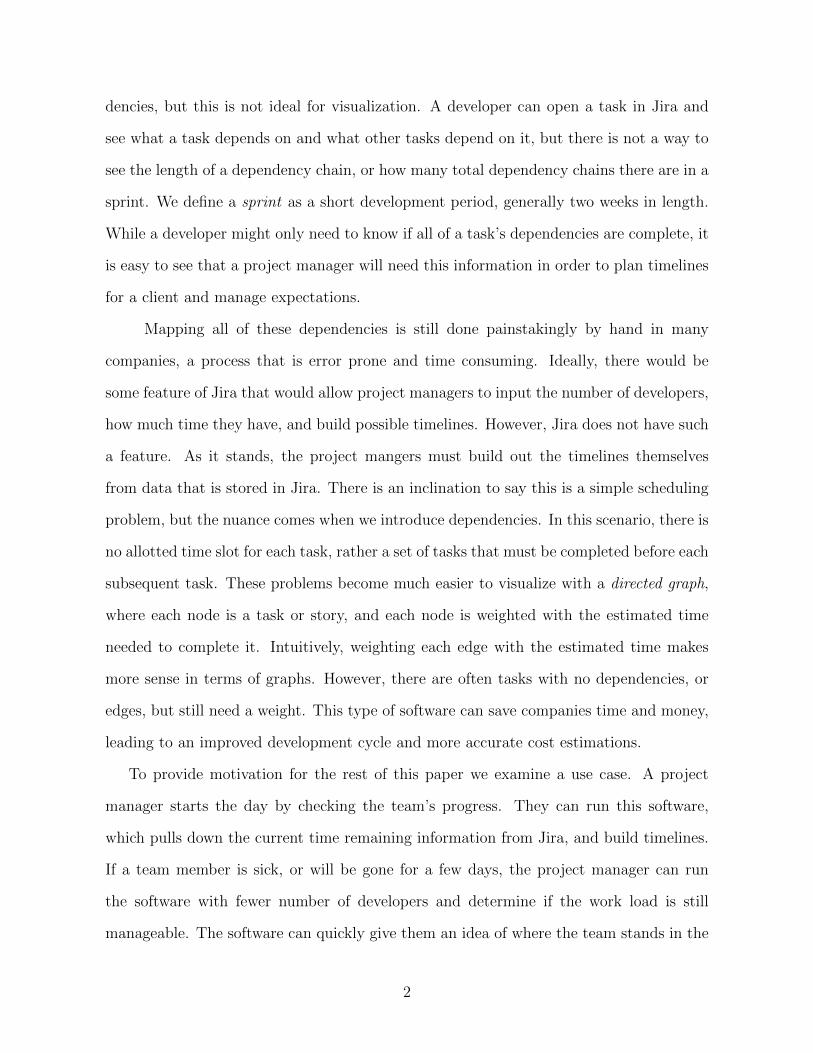
with its user interface, inputting tasks and starting sprints. One of the features of Jira is
the ability to link tasks. Figure 1.1 is a screenshot of Jira’s task display. Notice that when
Figure 1.1: Jira Task Display
two tasks are linked together, viewing details on one task will display the identifier of the
3
linked task and the user can click on the identifier to open the details page of the linked
task. While all of a task’s dependencies can be viewed, there is no way to see the entire
dependency chain without clicking through each link and recording them by hand. Jira
has extensive REST APIs that can help organize this information. A developer can use
these APIs to both pull down and push data to a Jira account with some authorization
tokens.
1.3 Related Work
The Program Evaluation and Review Technique (PERT) is a project management
methodology that aligns closely with this problem. PERT was created in 1957 for use in
the US Navy’s Polaris nuclear submarine project. It focuses on large complex projects
with many dependencies [3]. It gives a systematic approach to planning a project and
estimating total completion time.
To use PERT, we first establish all tasks of a project and determine the order in which
the tasks must be completed. Then time estimates are assigned to each task. Each task
has three times assigned to it: optimistic time, pessimistic time, and most likely time.
These separate times are used to calculate the expected time with the following equation:
Texpected = 16(Toptimistic + 4Tmost likely + Tpessimistic)
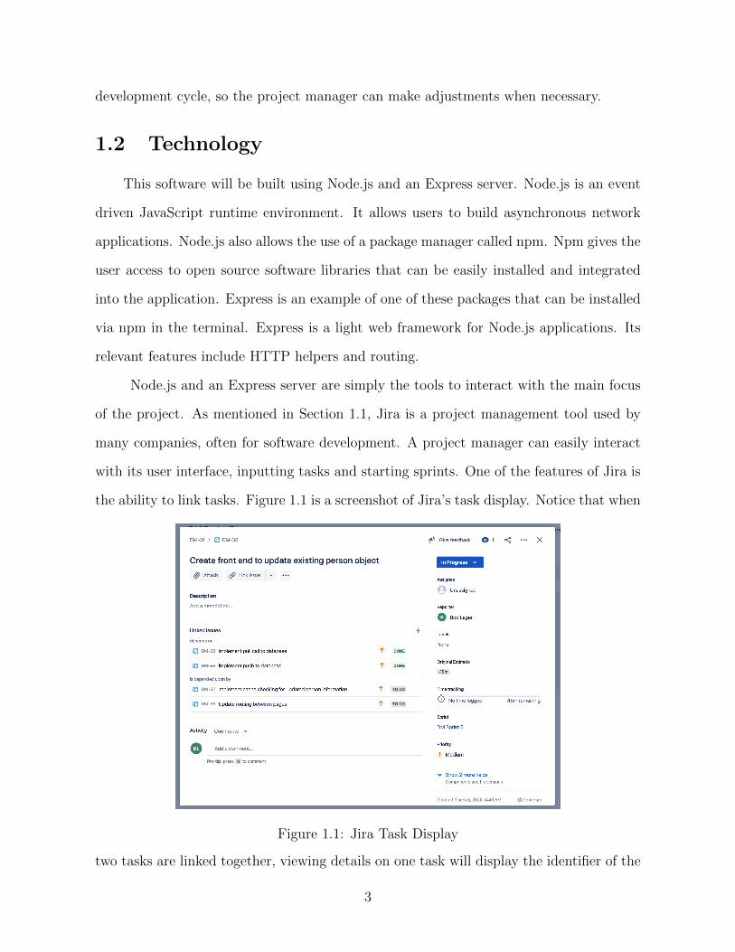
From there we create a network diagram of the tasks. The diagram displays tasks as
nodes and dependencies as lines, as shown in Figure 1.2.
The diagram contains a node called start, this activity has a duration of zero. An
activity is the actual act of performing a task, which consumes time and resources. Then
initial activities are connected to the start node with an arrow. The diagram will generally
display the name, estimated time, early start time, early finish time, late start time, late
finish time, and the slack for each activity. Slack is the amount of time a task can be
delayed without causing a delay in subsequent tasks or the project as a whole.
4
Figure 1.2: Example PERT Chart
Assume we have the estimated time (ET) for each activity. The early start time (EST)
will be the maximum early finish time (EFT) of all activities that proceed it. The early
start time for the first activity is zero. Early finish time is defined as the early start time
plus the estimated time. The late finish time (LFT) is the minimum late start of all the
activities succeeding it. If it is the last activity, the late finish equals the early finish.
The late start time (LST) is the late finish minus the estimated time. Notice the early
times must be computed before the late times. Then we can compute the available slack
for each task, slack (S) is the late start time minus the early start time. Below are the
equations to calculate each value.
EST = max(EFT of all proceeding tasks)
EFT = EST + ET
LFT = min(LST of all succeeding tasks)
LST = LFT − ET
S = LST − EST
Once these times are computed, we move to finding the critical path. The critical path is
the path that takes the longest time to complete. To find the time of a path, we sum the
estimated time for each task. With all task lengths computed, we can identify the critical
5

path as the path with the longest duration. The slack for the critical path will be zero.
6
2 Graph Theory
Before constructing the software itself, the mathematics behind the problem must
be examined. These dependency maps with which we will be working can be classified
as disconnected, weighted, directed graphs. It is important to note that we must either
consider the nodes to be weighted or introduce an imaginary root node to think of the
edges as weighted.
Throughout this paper, vertices may be referred to as nodes and edges may be referred
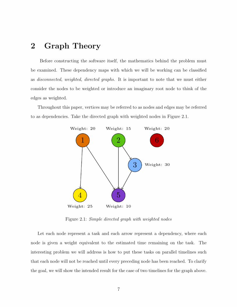
to as dependencies. Take the directed graph with weighted nodes in Figure 2.1.
Figure 2.1: Simple directed graph with weighted nodes
Let each node represent a task and each arrow represent a dependency, where each
node is given a weight equivalent to the estimated time remaining on the task. The
interesting problem we will address is how to put these tasks on parallel timelines such
that each node will not be reached until every preceding node has been reached. To clarify
the goal, we will show the intended result for the case of two timelines for the graph above.
7
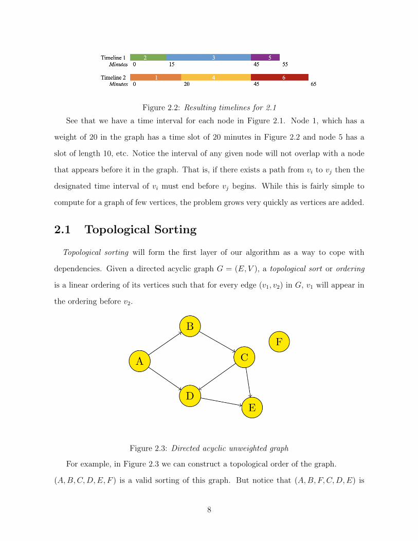
Figure 2.2: Resulting timelines for 2.1
See that we have a time interval for each node in Figure 2.1. Node 1, which has a
weight of 20 in the graph has a time slot of 20 minutes in Figure 2.2 and node 5 has a
slot of length 10, etc. Notice the interval of any given node will not overlap with a node
that appears before it in the graph. That is, if there exists a path from vi to vj then the
designated time interval of vi must end before vj begins. While this is fairly simple to
compute for a graph of few vertices, the problem grows very quickly as vertices are added.
2.1 Topological Sorting
Topological sorting will form the first layer of our algorithm as a way to cope with
dependencies. Given a directed acyclic graph G = (E, V ), a topological sort or ordering
is a linear ordering of its vertices such that for every edge (v1, v2) in G, v1 will appear in
the ordering before v2.
Figure 2.3: Directed acyclic unweighted graph
For example, in Figure 2.3 we can construct a topological order of the graph.
(A,B,C,D,E, F ) is a valid sorting of this graph. But notice that (A,B, F, C,D,E) is
8
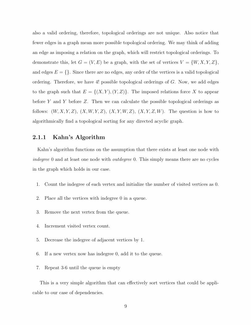
also a valid ordering, therefore, topological orderings are not unique. Also notice that
fewer edges in a graph mean more possible topological ordering. We may think of adding
an edge as imposing a relation on the graph, which will restrict topological orderings. To
demonstrate this, let G = (V,E) be a graph, with the set of vertices V = {W,X, Y, Z},
and edges E = {}. Since there are no edges, any order of the vertices is a valid topological
ordering. Therefore, we have 4! possible topological orderings of G. Now, we add edges
to the graph such that E = {(X, Y ), (Y, Z)}. The imposed relations force X to appear
before Y and Y before Z. Then we can calculate the possible topological orderings as
follows: (W,X, Y, Z), (X,W, Y, Z), (X, Y,W,Z), (X, Y, Z,W ). The question is how to
algorithmically find a topological sorting for any directed acyclic graph.
2.1.1 Kahn’s Algorithm
Kahn’s algorithm functions on the assumption that there exists at least one node with
indegree 0 and at least one node with outdegree 0. This simply means there are no cycles
in the graph which holds in our case.
1. Count the indegree of each vertex and initialize the number of visited vertices as 0.
2. Place all the vertices with indegree 0 in a queue.
3. Remove the next vertex from the queue.
4. Increment visited vertex count.
5. Decrease the indegree of adjacent vertices by 1.
6. If a new vertex now has indegree 0, add it to the queue.
7. Repeat 3-6 until the queue is empty
This is a very simple algorithm that can effectively sort vertices that could be appli-
cable to our case of dependencies.
9
2.2 Interval Scheduling Problem
The interval scheduling problem can be described as having a set of tasks that each can
only be completed during a given interval and the goal is to complete as many tasks as
possible. If a task overlaps with another, they cannot both be completed. The algorithm
to solve this problem is quite simple. First, the tasks are sorted based on end time. Then,
select the first task and eliminate tasks that overlap with the selected task. This selection
and elimination process is repeated until all tasks have been selected or eliminated.
10
3 Design
3.1 Initial Construction
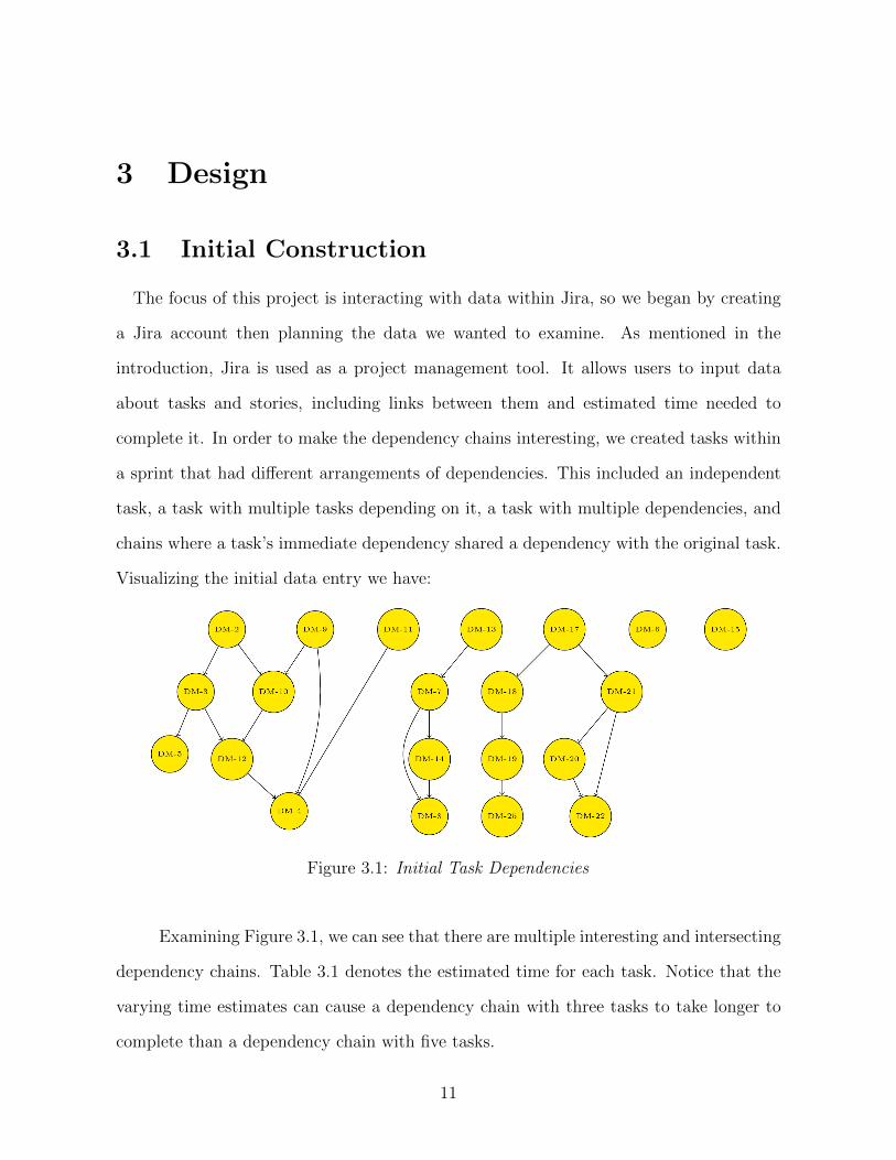
The focus of this project is interacting with data within Jira, so we began by creating
a Jira account then planning the data we wanted to examine. As mentioned in the
introduction, Jira is used as a project management tool. It allows users to input data
about tasks and stories, including links between them and estimated time needed to
complete it. In order to make the dependency chains interesting, we created tasks within
a sprint that had different arrangements of dependencies. This included an independent
task, a task with multiple tasks depending on it, a task with multiple dependencies, and
chains where a task’s immediate dependency shared a dependency with the original task.
Visualizing the initial data entry we have:
Figure 3.1: Initial Task Dependencies
Examining Figure 3.1, we can see that there are multiple interesting and intersecting
dependency chains. Table 3.1 denotes the estimated time for each task. Notice that the
varying time estimates can cause a dependency chain with three tasks to take longer to
complete than a dependency chain with five tasks.
11
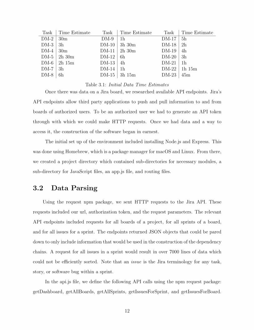
Task Time Estimate Task Time Estimate Task Time EstimateDM-2 30m DM-9 1h DM-17 5hDM-3 3h DM-10 3h 30m DM-18 2hDM-4 30m DM-11 2h 30m DM-19 4hDM-5 2h 30m DM-12 6h DM-20 3hDM-6 2h 15m DM-13 4h DM-21 1hDM-7 3h DM-14 1h DM-22 1h 15mDM-8 6h DM-15 3h 15m DM-23 45m
Table 3.1: Initial Data Time Estimates
Once there was data on a Jira board, we researched available API endpoints. Jira’s
API endpoints allow third party applications to push and pull information to and from
boards of authorized users. To be an authorized user we had to generate an API token
through with which we could make HTTP requests. Once we had data and a way to
access it, the construction of the software began in earnest.
The initial set up of the environment included installing Node.js and Express. This
was done using Homebrew, which is a package manager for macOS and Linux. From there,
we created a project directory which contained sub-directories for necessary modules, a
sub-directory for JavaScript files, an app.js file, and routing files.
3.2 Data Parsing
Using the request npm package, we sent HTTP requests to the Jira API. These
requests included our url, authorization token, and the request parameters. The relevant
API endpoints included requests for all boards of a project, for all sprints of a board,
and for all issues for a sprint. The endpoints returned JSON objects that could be pared
down to only include information that would be used in the construction of the dependency
chains. A request for all issues in a sprint would result in over 7000 lines of data which
could not be efficiently sorted. Note that an issue is the Jira terminology for any task,
story, or software bug within a sprint.
In the api.js file, we define the following API calls using the npm request package:
getDashboard, getAllBoards, getAllSprints, getIssuesForSprint, and getIssuesForBoard.
12
These requests return JavaScript promises that will resolve to a JSON object containing
data. Within the parser.js file, we used these functions and proceeded to pull the necessary
information off of the JSON object. The parsed information was then returned as a
promise.
Parsing getAllBoards will return a promise, which resolves to a JSON object con-
taining the id, name, project key, and project name of the board. Parsing getSprints will
return a promise which resolves to a JSON object containing the id, state (active, future,
or completed), name, start date, end date, and boardId of the sprint. The objective of
parsing boards and sprints is to find boards containing active sprints. Once the IDs of
active sprints are found, we can parse getIssuesForSprint to find the information needed
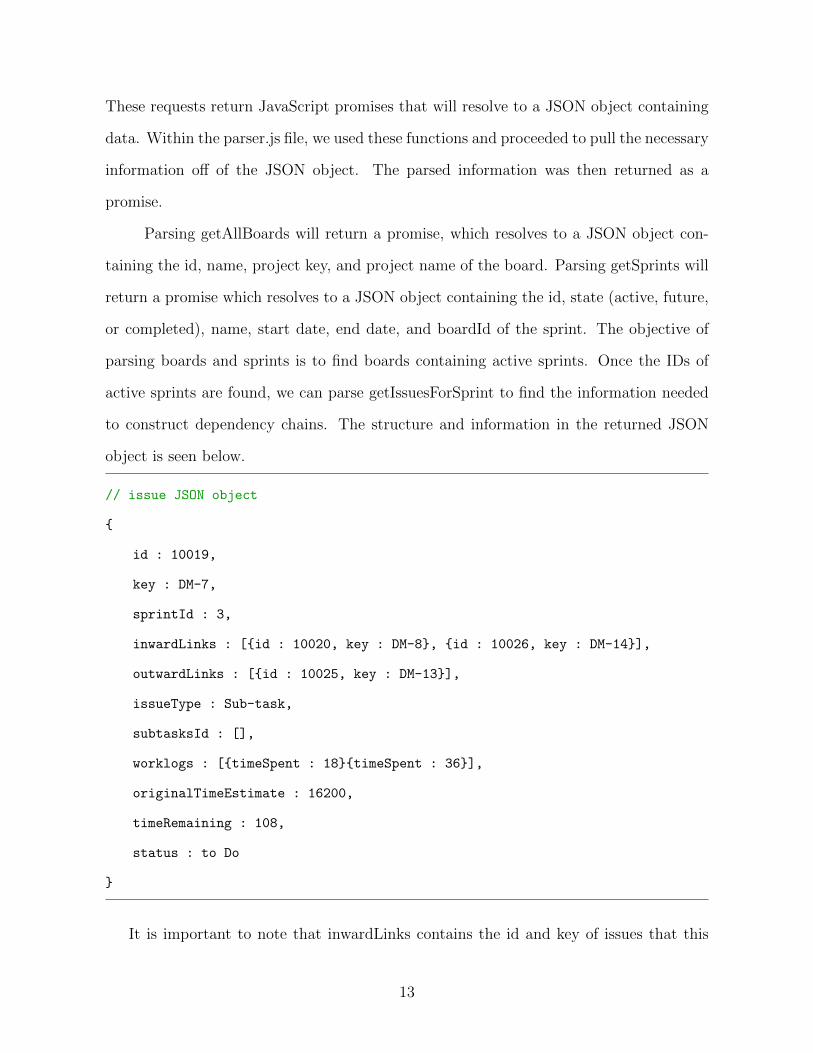
to construct dependency chains. The structure and information in the returned JSON
object is seen below.
// issue JSON object
{
id : 10019,
key : DM-7,
sprintId : 3,
inwardLinks : [{id : 10020, key : DM-8}, {id : 10026, key : DM-14}],
outwardLinks : [{id : 10025, key : DM-13}],
issueType : Sub-task,
subtasksId : [],
worklogs : [{timeSpent : 18}{timeSpent : 36}],
originalTimeEstimate : 16200,
timeRemaining : 108,
status : to Do
}
It is important to note that inwardLinks contains the id and key of issues that this
13
issue is depended upon by and outwardLinks contains the id and key of issues that this
issue depends on. For example, consider the data in Figure 3.1. The inwardLinks array
for DM-7 would include DM-14 and DM-8, while the outwardLinks array would contain
DM-13.
There were some problems when initially parsing this data since the necessary pieces
of information were often in very nested objects and if there was no available data in
an object, there would be undefined errors that had to be handled. Issue type was
occasionally a field that could not be accessed. Examples of issue types are task, sub-
task, bug, and story.
3.3 Construction of Dependency Chains
Before constructing dependency chains, we had to turn the parsed objects into easily
accessible information. Since each issue had a unique key, we decided to feed all the issue
objects into a map using the issue key as the map key. We did this in the buildMap
function. In the buildMap function we called getBoards, then pulled the board id off
the response object and used it to call getSprints. The response object for getSprints
contained the sprint ids which were finally used to call getIssuesForSprint. From there we
looped through each issue and created an entry on the map.
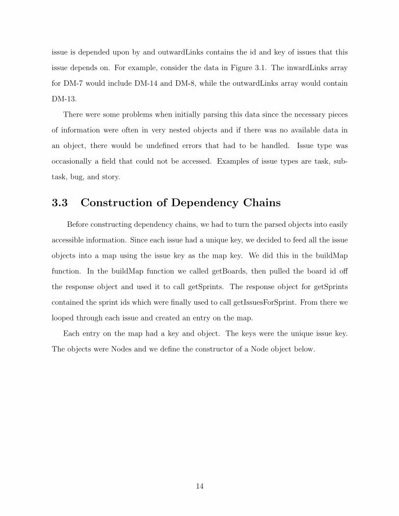
Each entry on the map had a key and object. The keys were the unique issue key.
The objects were Nodes and we define the constructor of a Node object below.
14
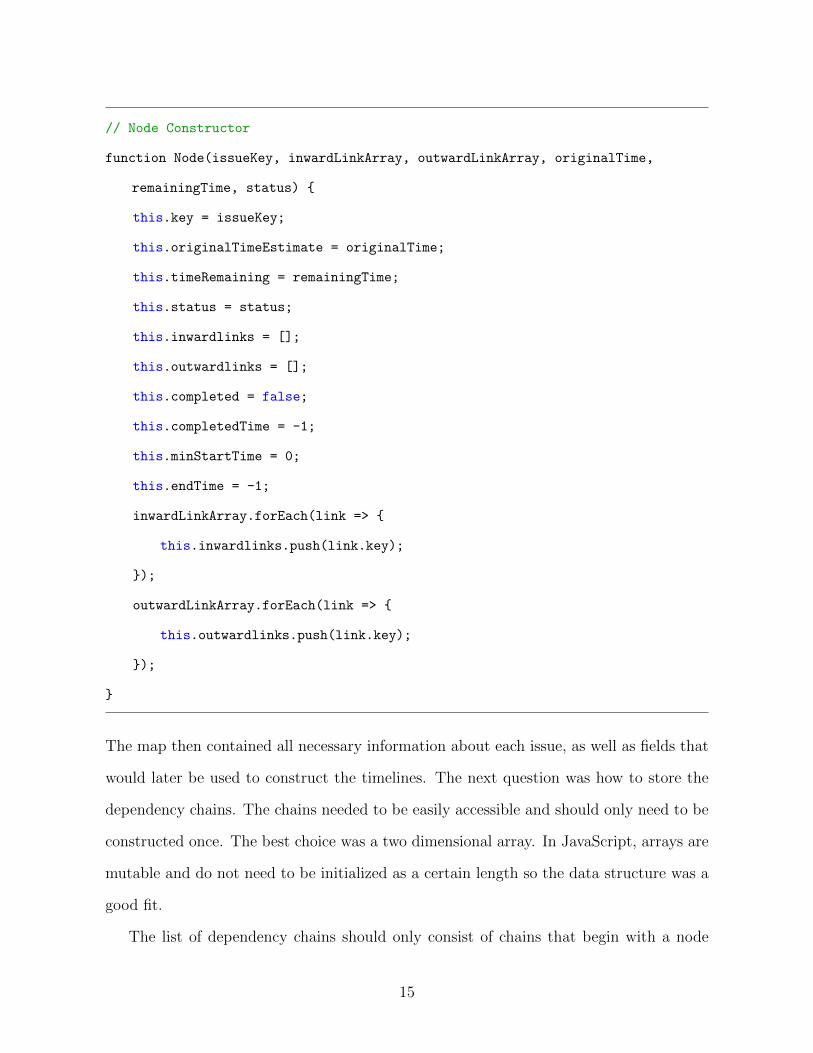
// Node Constructor
function Node(issueKey, inwardLinkArray, outwardLinkArray, originalTime,
remainingTime, status) {
this.key = issueKey;
this.originalTimeEstimate = originalTime;
this.timeRemaining = remainingTime;
this.status = status;
this.inwardlinks = [];
this.outwardlinks = [];
this.completed = false;
this.completedTime = -1;
this.minStartTime = 0;
this.endTime = -1;
inwardLinkArray.forEach(link => {
this.inwardlinks.push(link.key);
});
outwardLinkArray.forEach(link => {
this.outwardlinks.push(link.key);
});
}
The map then contained all necessary information about each issue, as well as fields that
would later be used to construct the timelines. The next question was how to store the
dependency chains. The chains needed to be easily accessible and should only need to be
constructed once. The best choice was a two dimensional array. In JavaScript, arrays are
mutable and do not need to be initialized as a certain length so the data structure was a
good fit.
The list of dependency chains should only consist of chains that begin with a node
15
that does not depend on any other node and terminates only when the last node in the
chain does not have any nodes that depend on it. That is, considering Figure 3.1, DM-13
→ DM-7 → DM-14 → DM-8 is a valid dependency chain but DM-7 → DM-14 is not a
valid dependency chain. To ensure we only included valid dependency chains, we had to
loop through all the nodes and create an array consisting of nodes whose outwardLink
array had a length of 0. We called this the root array and for each root node we called the
recursive function buildArrayOfDependencies. This function takes in the map of nodes,
a node key, an array, and a time. To build the chains, the function pushes the key into
the array. It checks for dependencies by looking if the length of the inwardLink array is
0. If length is not 0 then there is another node that depends on the current node and we
recursively call the buildArrayOfDependencies method and pass the key of the dependent
node, the node map, the array with the current node pushed to it, and the time for the
chain. When a node is reached that does have an inwardLink array of length 0, meaning
there are no other nodes that depend on it, the function will push to total time of the
chain onto the array and return the array.
Calling the buildArrayOfDependencies function results in a global array called de-
pendencyChains. Each entry in the array is another array which represents a different
dependency chain. The final entry in each dependency chain array is the total estimated
time to complete the dependency chain. The dependencyChains array will be used directly
in the dependency mapping algorithm.
3.4 Dependency Mapping Algorithm
The focus of this project is the dependency mapping algorithm. We wanted to allow
project managers to quickly determine the workload a team could complete, and create
viable timelines for reference. The simple first case for this is: given an infinite amount of
developers, how quickly can a set of tasks be completed. We implemented this functional-
ity in the minTimeUnlimitedDevelopers function. Analyzing this problem, we see that we
16
can distribute each independent task to a different developer and their completion times
will match with their estimated time. Hence, if this function is given a set of completely
independent tasks the result should be time estimate of the largest task. However, if there
are dependencies within the tasks more information must be considered. The question is
how to handle these dependencies and ensure that they are completed efficiently.
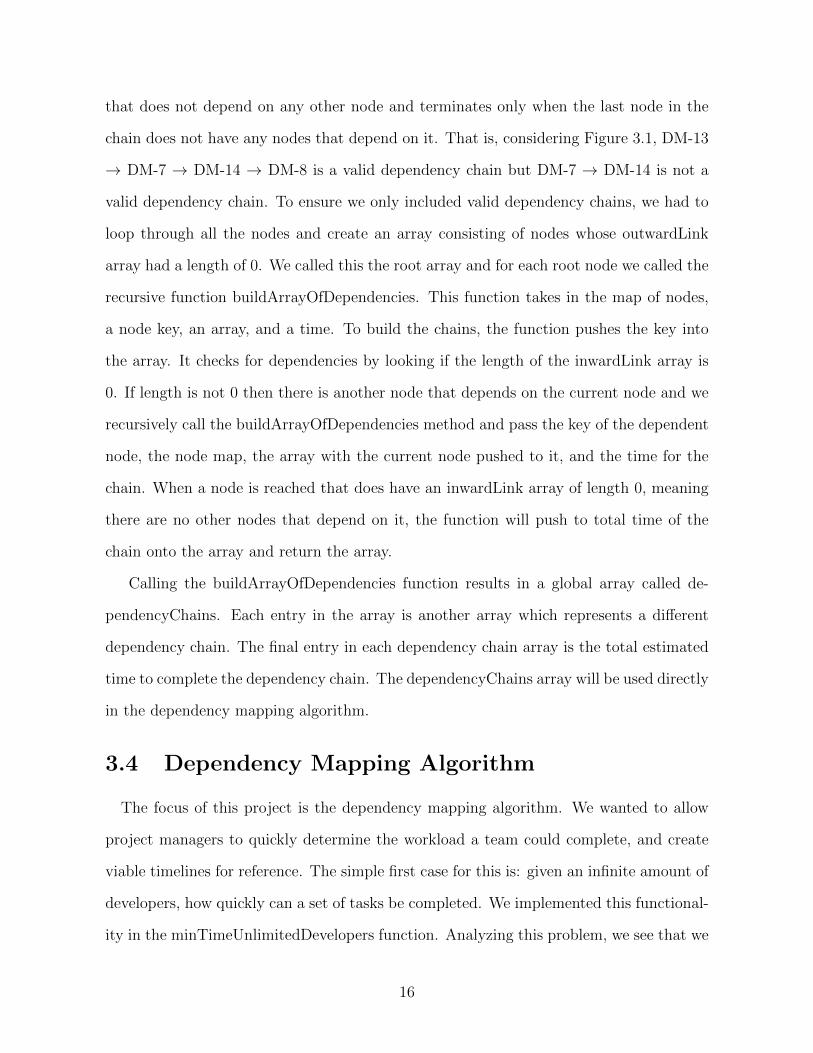
Figure 3.2: Test Data for Unlimited Developers
Consider the tasks in Figure 3.2. It is clear that it will take longer than the longest
individual task to complete the set of tasks. This is true as 4 must be completed before
5, 6, and 7 can be started. Notice that the restrictions on the order can be examined in
terms of dependency chains. That is, if we constructed each possible dependency chain
and gave each chain to a different developer we could ensure each task is completed as
soon as possible. This distribution of tasks would contain repeated tasks so we would
need to remove all but the latest occurrence of a task.
To understand this process take all the dependency chains in Figure 3.2: [1, 4, 5],
[1, 4, 6, 7], [2, 4, 5], [2, 4, 6, 7], [3, 6, 7], [3, 7]. We give each developer a dependency chain
and keep track of the start time of each task in the chain. We define the start time of a
task as the sum of time estimates of all the tasks appearing before it in the chain. Then
we remove each repeated task leaving the copy with the latest start time. If we do not
recompute the start times of the tasks, we are left with a timeline for each developer
17
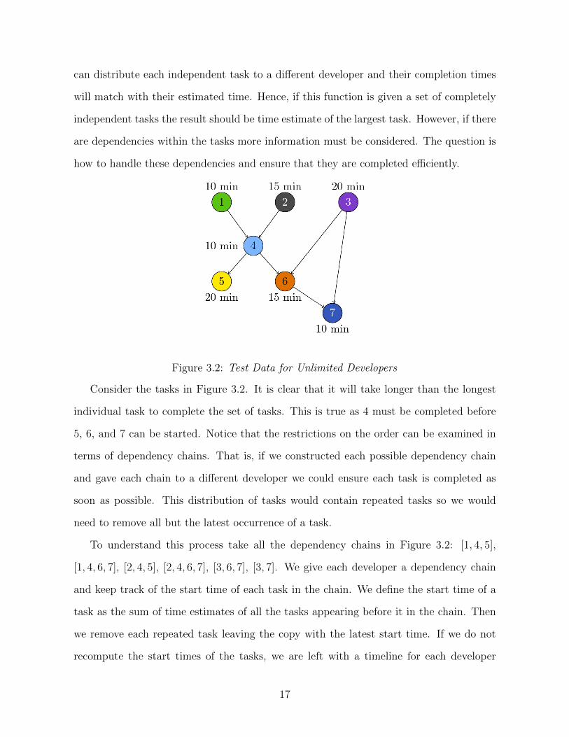
where all dependencies for a task are completed before we reach the dependent task.
Figure 3.3: Timelines for Unlimited Developers Pre-removal
Figure 3.3 shows the corresponding timeline for each dependency chain. Developer 6
is meant to start on task 7 at 20 minutes, but notice that all the tasks 7 is dependent on
will not be completed until 40 minutes. This is why we must remove all copies of a task
except the latest occurring task.
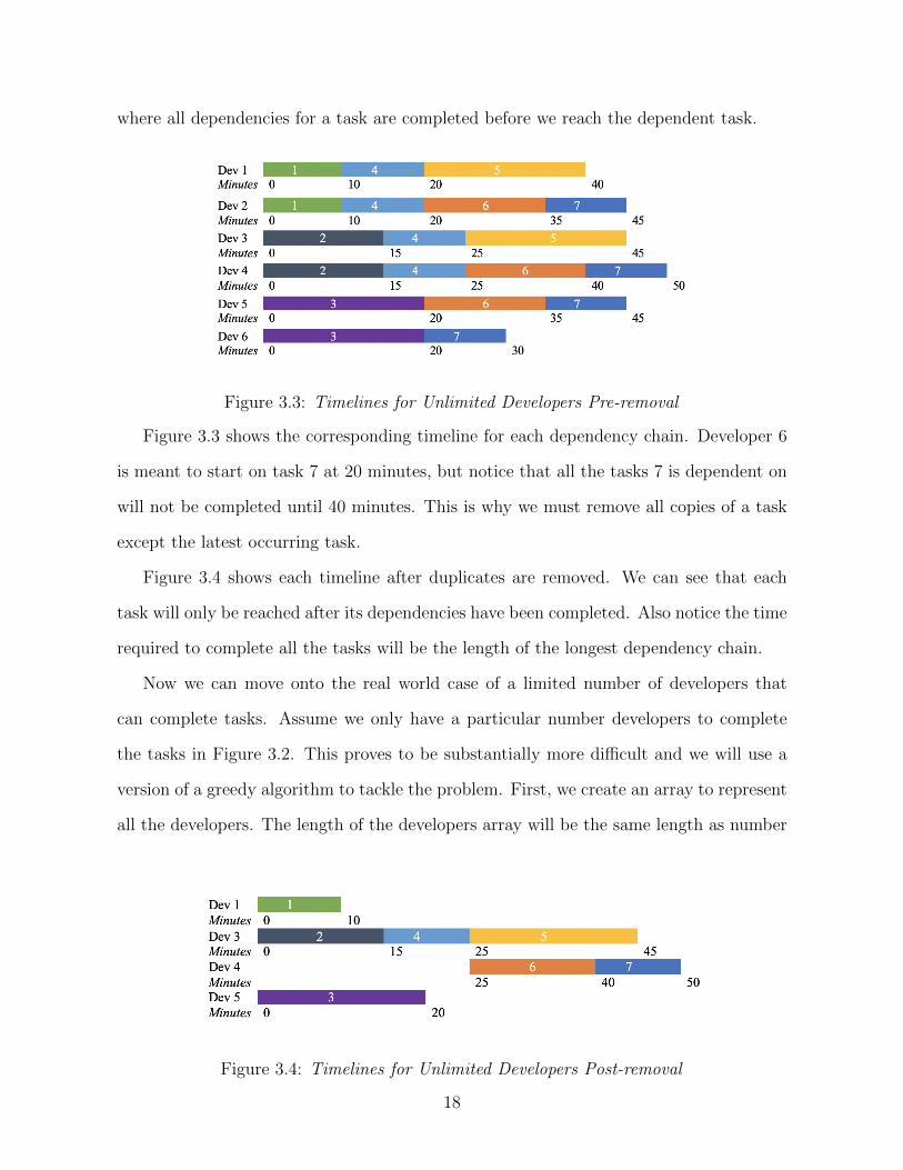
Figure 3.4 shows each timeline after duplicates are removed. We can see that each
task will only be reached after its dependencies have been completed. Also notice the time
required to complete all the tasks will be the length of the longest dependency chain.
Now we can move onto the real world case of a limited number of developers that
can complete tasks. Assume we only have a particular number developers to complete
the tasks in Figure 3.2. This proves to be substantially more difficult and we will use a
version of a greedy algorithm to tackle the problem. First, we create an array to represent
all the developers. The length of the developers array will be the same length as number
Figure 3.4: Timelines for Unlimited Developers Post-removal
18
of developers. From there we create two maps of nodes, an empty map representing all
completed tasks and a map containing all the incomplete tasks. Initially the map of
incomplete tasks will contain all the tasks in the original node map. Recall the interval
scheduling problem discussed in section 2.3. The algorithm used to solve this problem
requires us to know the end times of each task. So we can check the earliest end time for
each task but this requires some extra thought in the limited developers case.
Recall that all dependencies of a task must be completed before a task can be started.
But also recall that limiting the number of developers will cause some tasks’ start times
to be pushed back. Therefore, we must calculate the latest end time for any dependency
of a task and add the estimated time for the task to determine the earliest a task can
be completed. We denote the length of a task G as |G|, the completed time as TG, and
the earliest end time, Gend. The earliest possible end time is computed purely based on
length of tasks and their dependencies, while completed time is computed as tasks are
assigned to developers. Notice when we restrict the number of developers, a task can have
a later completed time than its earliest possible end time. For example, let A be a task,
which is dependent on tasks B and C. It is calculated that B will be completed at time
TB = 30min, however C will not be completed until time TC = 40min. Since TB < TC ,
Aend = |A|+ TC .
So we determine the earliest end time of all the incomplete tasks and choose the task
with the earliest end time, we denote this task A. We denote the amount of time currently
allotted to a developer d as |d|. Then we determine which developer should take the task.
We give the task to the developer di such that |di| ≥ Aend−|A| and if there exists dk such
that |dk| < |di| then |dk| � Aend − |A|. To state this informally, we select the developer
with the smallest amount of time worked such that time worked is greater than or equal
to the earliest start time of the task. Then we give the task to the developer, update the
developer with a new time worked, remove the task from the incomplete map and put the
task in the completed map. This process is repeated until the incomplete map is empty.
19
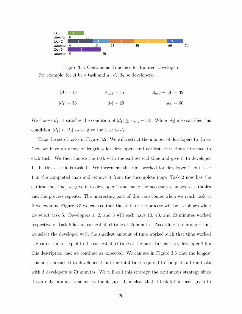
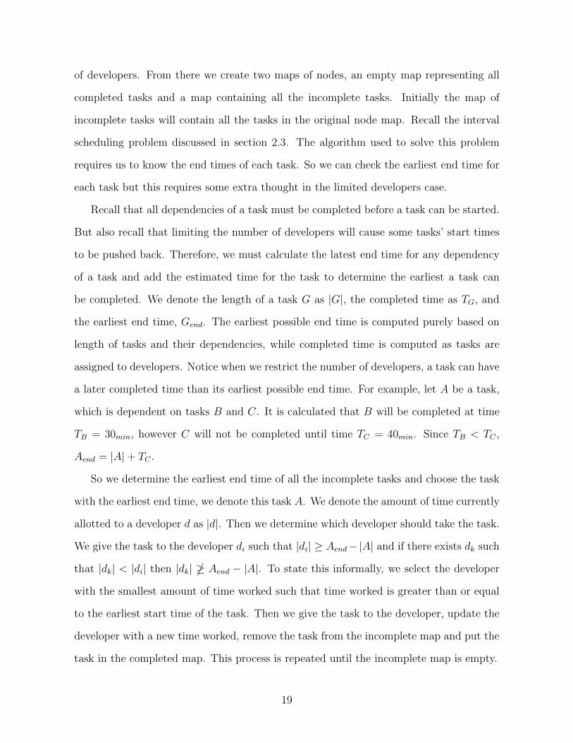
Figure 3.5: Continuous Timelines for Limited Developers
For example, let A be a task and d1, d2, d3 be developers.
|A| = 13 Aend = 45 Aend − |A| = 32
|d1| = 38 |d2| = 29 |d3| = 60
We choose d1, it satisfies the condition of |d1| ≥ Aend − |A|. While |d3| also satisfies this
condition, |d1| < |d3| so we give the task to d1.
Take the set of tasks in Figure 3.2. We will restrict the number of developers to three.
Now we have an array of length 3 for developers and earliest start times attached to
each task. We then choose the task with the earliest end time and give it to developer
1. In this case it is task 1. We increment the time worked for developer 1, put task
1 in the completed map and remove it from the incomplete map. Task 2 now has the
earliest end time, we give it to developer 2 and make the necessary changes to variables
and the process repeats. The interesting part of this case comes when we reach task 5.
If we examine Figure 3.5 we can see that the state of the process will be as follows when
we select task 5. Developers 1, 2, and 3 will each have 10, 40, and 20 minutes worked
respectively. Task 5 has an earliest start time of 25 minutes. According to our algorithm,
we select the developer with the smallest amount of time worked such that time worked
is greater than or equal to the earliest start time of the task. In this case, developer 2 fits
this description and we continue as expected. We can see in Figure 3.5 that the longest
timeline is attached to developer 2 and the total time required to complete all the tasks
with 3 developers is 70 minutes. We will call this strategy the continuous strategy since
it can only produce timelines without gaps. It is clear that if task 5 had been given to
20
developer 3, leaving a gap in developer 3’s timeline, we could produce a smaller total time.
Figure 3.6: Discontinuous Timelines for Limited Developers
There is a fairly simple tweak to the choice of developer criterion which will help
handle cases of this nature. Again, let A be a task and di be a developer. We give A to
the developer di such that |di| = Aend − |A| and if no such di exists then we choose di
such that there does not exist dk such that ||dk| − (Aend − |A|)| < ||di| − (Aend − |A|)|.
For example, we again examine a task A and developers d1, d2, d3.
|A| = 13 Aend = 45 Aend − |A| = 32
|d1| = 38 |d2| = 29 |d3| = 60
In this case we choose d2 since
||d2| − (Aend − |A|)| < ||d3| − (Aend − |A|)|
|29− 32| < |38− 32|
3 < 6
When we take this strategy change into account we get a better result from our algorithm
as seen in Figure 3.6. Notice that task 5 has been moved to developer 3 which allows
task 7 to be completed 20 minutes earlier. We will call this strategy the discontinuous
strategy. While this change in choice criterion improved the results in this set of tasks, we
will see that there are cases where the continuous method produces a better result than
the discontinuous strategy and vice versa. These cases will be examined in Section 4.
21
3.5 Front End Development
The original intention of this software was that it would be hosted on a web platform
with a UI for project managers. We began running the software on an Express server which
we planned to later transition to a more permanent web server, Turing for example. Once
we felt the software should be moved to Turing, and the front end developed we discovered
that web platforms do not support some of the Node.js functions that were used during
development. The main problem being ’require’ statements that were used to connect all
the different pieces of the program.
From there we decided to switch gears and create a simple terminal interface that
would allow a project manager to input the various sprints on which they wanted to run
calculations and what analysis they wanted done. To display the dependency chains, we
simply print the total time of a dependency chain and below it, the tasks in the chain,
in order, separated by arrows. The output for timelines is fairly simple, but intuitive.
For each developer, there will be a line that states the total time for the timeline. The
total time is computed as the end time for the last task the developer completes. Then
the line below that displays all the tasks in a row. It shows the start time for the task,
the name of the task, then the completion time for the task. Gaps in timelines are not
particularly noticeable, but since both the start and end times are shown for each task,
gaps in work can be seen as differences between the end time of a task, and the start time
of the following task. The most reasonable extension for the front end in the future would
be to output JPEGs of the dependency chains and the timeline for the developers.
22
4 Testing and Results
To understand the good and the bad of the strategies, we will run both algorithms on
various test data with different parameters. The test data is assigned an alphanumeric
tag by Jira. The test project was named ’Dependency Mapper’ in Jira, so tasks in the
project are tagged with ’DM’. We will begin by examining the algorithm’s performance
on the simplest case, the set of tasks with no dependencies.
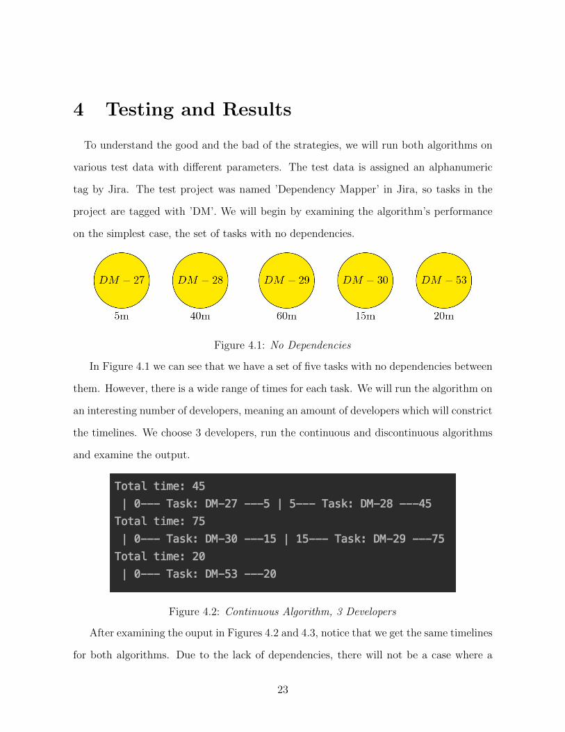
Figure 4.1: No Dependencies
In Figure 4.1 we can see that we have a set of five tasks with no dependencies between
them. However, there is a wide range of times for each task. We will run the algorithm on
an interesting number of developers, meaning an amount of developers which will constrict
the timelines. We choose 3 developers, run the continuous and discontinuous algorithms
and examine the output.
Figure 4.2: Continuous Algorithm, 3 Developers
After examining the ouput in Figures 4.2 and 4.3, notice that we get the same timelines
for both algorithms. Due to the lack of dependencies, there will not be a case where a
23
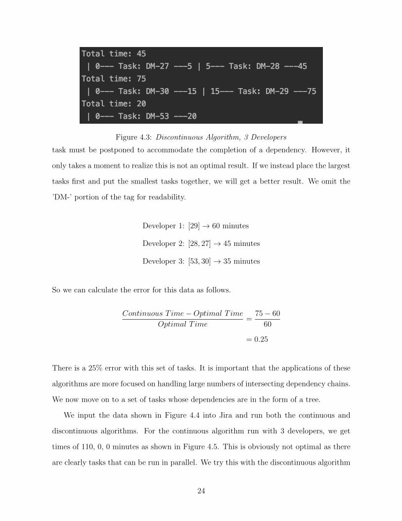
Figure 4.3: Discontinuous Algorithm, 3 Developers
task must be postponed to accommodate the completion of a dependency. However, it
only takes a moment to realize this is not an optimal result. If we instead place the largest
tasks first and put the smallest tasks together, we will get a better result. We omit the
’DM-’ portion of the tag for readability.
Developer 1: [29]→ 60 minutes
Developer 2: [28, 27]→ 45 minutes
Developer 3: [53, 30]→ 35 minutes
So we can calculate the error for this data as follows.
Continuous T ime−Optimal T ime
Optimal T ime=
75− 60
60
= 0.25
There is a 25% error with this set of tasks. It is important that the applications of these
algorithms are more focused on handling large numbers of intersecting dependency chains.
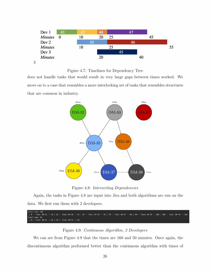
We now move on to a set of tasks whose dependencies are in the form of a tree.
We input the data shown in Figure 4.4 into Jira and run both the continuous and
discontinuous algorithms. For the continuous algorithm run with 3 developers, we get
times of 110, 0, 0 minutes as shown in Figure 4.5. This is obviously not optimal as there
are clearly tasks that can be run in parallel. We try this with the discontinuous algorithm
24
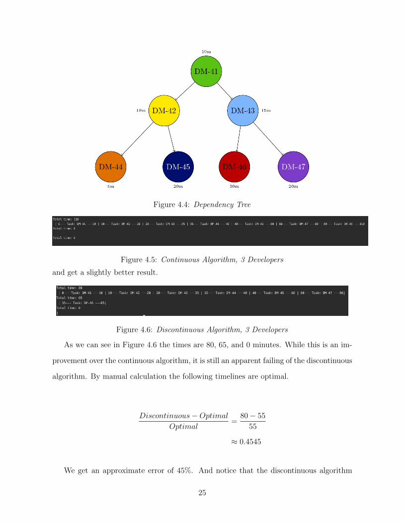
Figure 4.4: Dependency Tree
Figure 4.5: Continuous Algorithm, 3 Developers
and get a slightly better result.
Figure 4.6: Discontinuous Algorithm, 3 Developers
As we can see in Figure 4.6 the times are 80, 65, and 0 minutes. While this is an im-
provement over the continuous algorithm, it is still an apparent failing of the discontinuous
algorithm. By manual calculation the following timelines are optimal.
Discontinuous−Optimal
Optimal=
80− 55
55
≈ 0.4545
We get an approximate error of 45%. And notice that the discontinuous algorithm
25
3
Figure 4.7: Timelines for Dependency Tree
does not handle tasks that would result in very large gaps between times worked. We
move on to a case that resembles a more interlocking set of tasks that resembles structures
that are common in industry.
Figure 4.8: Intersecting Dependencies
Again, the tasks in Figure 4.8 are input into Jira and both algorithms are run on the
data. We first run them with 2 developers.
Figure 4.9: Continuous Algorithm, 2 Developers
We can see from Figure 4.9 that the times are 160 and 50 minutes. Once again, the
discontinuous algorithm performed better than the continuous algorithm with times of
26
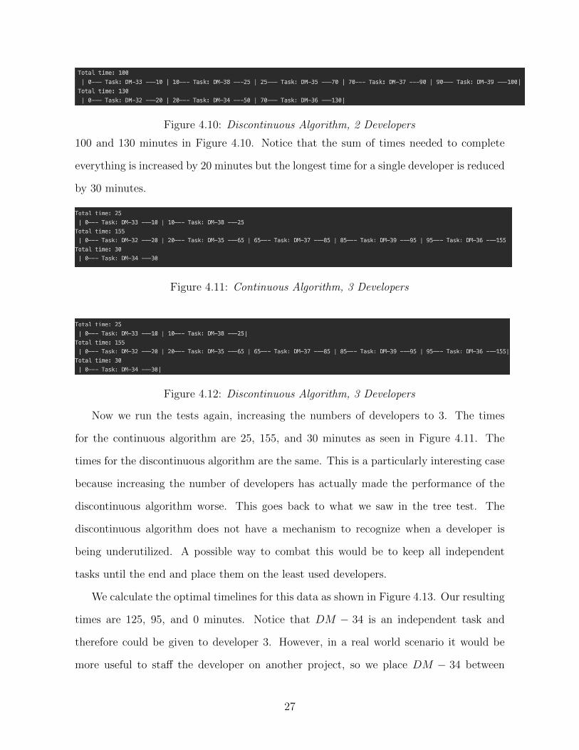
Figure 4.10: Discontinuous Algorithm, 2 Developers
100 and 130 minutes in Figure 4.10. Notice that the sum of times needed to complete
everything is increased by 20 minutes but the longest time for a single developer is reduced
by 30 minutes.
Figure 4.11: Continuous Algorithm, 3 Developers
Figure 4.12: Discontinuous Algorithm, 3 Developers
Now we run the tests again, increasing the numbers of developers to 3. The times
for the continuous algorithm are 25, 155, and 30 minutes as seen in Figure 4.11. The
times for the discontinuous algorithm are the same. This is a particularly interesting case
because increasing the number of developers has actually made the performance of the
discontinuous algorithm worse. This goes back to what we saw in the tree test. The
discontinuous algorithm does not have a mechanism to recognize when a developer is
being underutilized. A possible way to combat this would be to keep all independent
tasks until the end and place them on the least used developers.
We calculate the optimal timelines for this data as shown in Figure 4.13. Our resulting
times are 125, 95, and 0 minutes. Notice that DM − 34 is an independent task and
therefore could be given to developer 3. However, in a real world scenario it would be
more useful to staff the developer on another project, so we place DM − 34 between
27
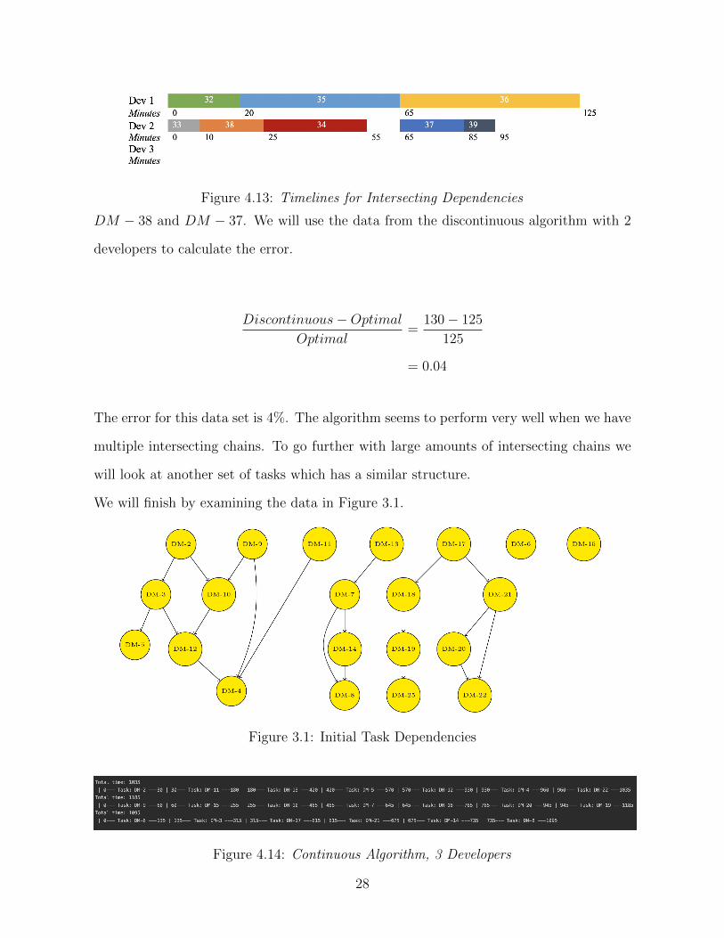
Figure 4.13: Timelines for Intersecting Dependencies
DM − 38 and DM − 37. We will use the data from the discontinuous algorithm with 2
developers to calculate the error.
Discontinuous−Optimal
Optimal=
130− 125
125
= 0.04
The error for this data set is 4%. The algorithm seems to perform very well when we have
multiple intersecting chains. To go further with large amounts of intersecting chains we
will look at another set of tasks which has a similar structure.
We will finish by examining the data in Figure 3.1.
Figure 3.1: Initial Task Dependencies
Figure 4.14: Continuous Algorithm, 3 Developers
28
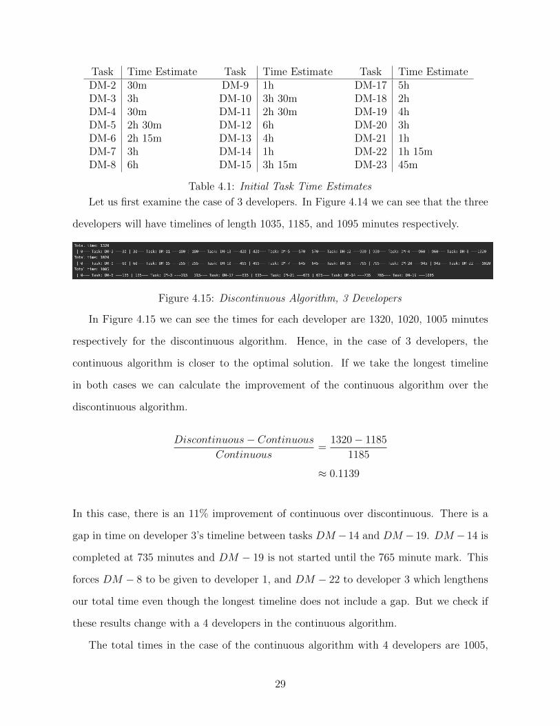
Task Time Estimate Task Time Estimate Task Time EstimateDM-2 30m DM-9 1h DM-17 5hDM-3 3h DM-10 3h 30m DM-18 2hDM-4 30m DM-11 2h 30m DM-19 4hDM-5 2h 30m DM-12 6h DM-20 3hDM-6 2h 15m DM-13 4h DM-21 1hDM-7 3h DM-14 1h DM-22 1h 15mDM-8 6h DM-15 3h 15m DM-23 45m
Table 4.1: Initial Task Time Estimates
Let us first examine the case of 3 developers. In Figure 4.14 we can see that the three
developers will have timelines of length 1035, 1185, and 1095 minutes respectively.
Figure 4.15: Discontinuous Algorithm, 3 Developers
In Figure 4.15 we can see the times for each developer are 1320, 1020, 1005 minutes
respectively for the discontinuous algorithm. Hence, in the case of 3 developers, the
continuous algorithm is closer to the optimal solution. If we take the longest timeline
in both cases we can calculate the improvement of the continuous algorithm over the
discontinuous algorithm.
Discontinuous− Continuous
Continuous=
1320− 1185
1185
≈ 0.1139
In this case, there is an 11% improvement of continuous over discontinuous. There is a
gap in time on developer 3’s timeline between tasks DM − 14 and DM − 19. DM − 14 is
completed at 735 minutes and DM − 19 is not started until the 765 minute mark. This
forces DM − 8 to be given to developer 1, and DM − 22 to developer 3 which lengthens
our total time even though the longest timeline does not include a gap. But we check if
these results change with a 4 developers in the continuous algorithm.
The total times in the case of the continuous algorithm with 4 developers are 1005,
29
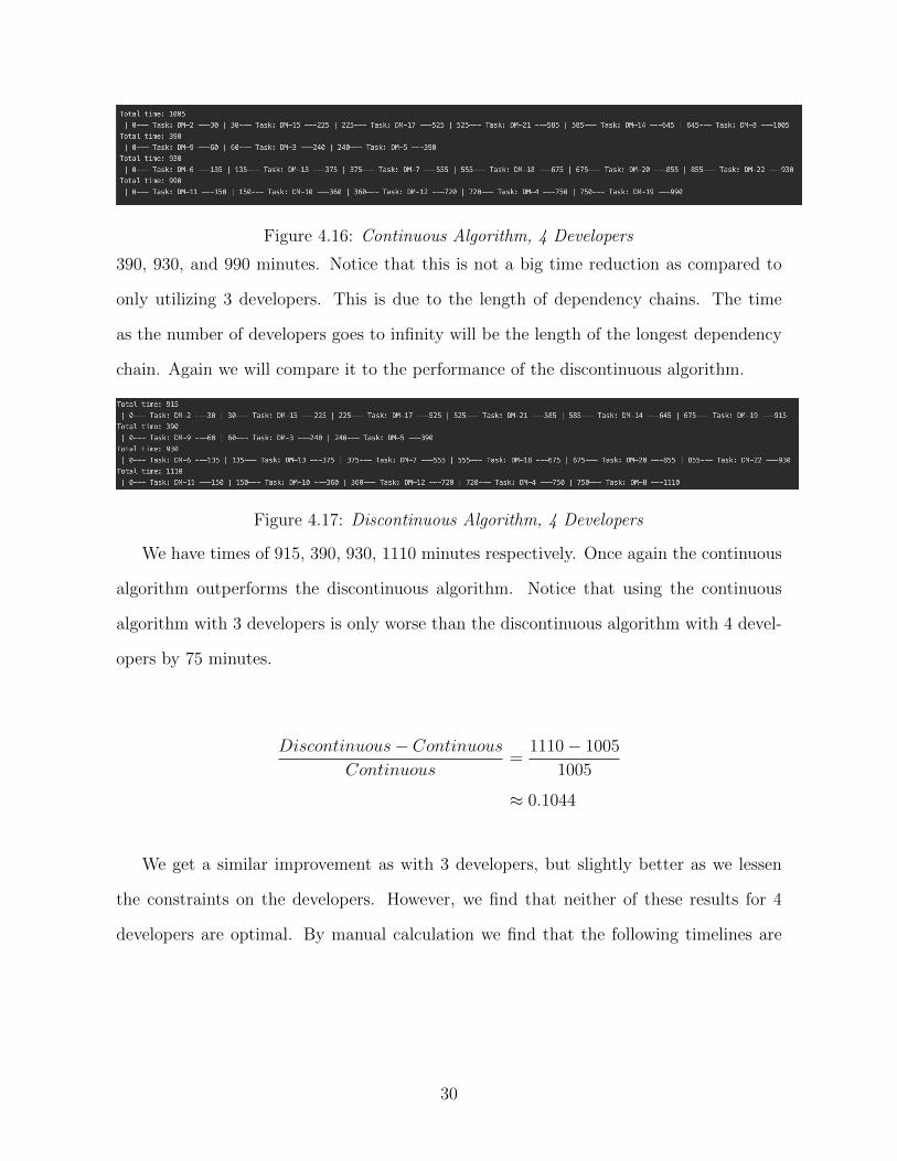
Figure 4.16: Continuous Algorithm, 4 Developers
390, 930, and 990 minutes. Notice that this is not a big time reduction as compared to
only utilizing 3 developers. This is due to the length of dependency chains. The time
as the number of developers goes to infinity will be the length of the longest dependency
chain. Again we will compare it to the performance of the discontinuous algorithm.
Figure 4.17: Discontinuous Algorithm, 4 Developers
We have times of 915, 390, 930, 1110 minutes respectively. Once again the continuous
algorithm outperforms the discontinuous algorithm. Notice that using the continuous
algorithm with 3 developers is only worse than the discontinuous algorithm with 4 devel-
opers by 75 minutes.
Discontinuous− Continuous
Continuous=
1110− 1005
1005
≈ 0.1044
We get a similar improvement as with 3 developers, but slightly better as we lessen
the constraints on the developers. However, we find that neither of these results for 4
developers are optimal. By manual calculation we find that the following timelines are
30
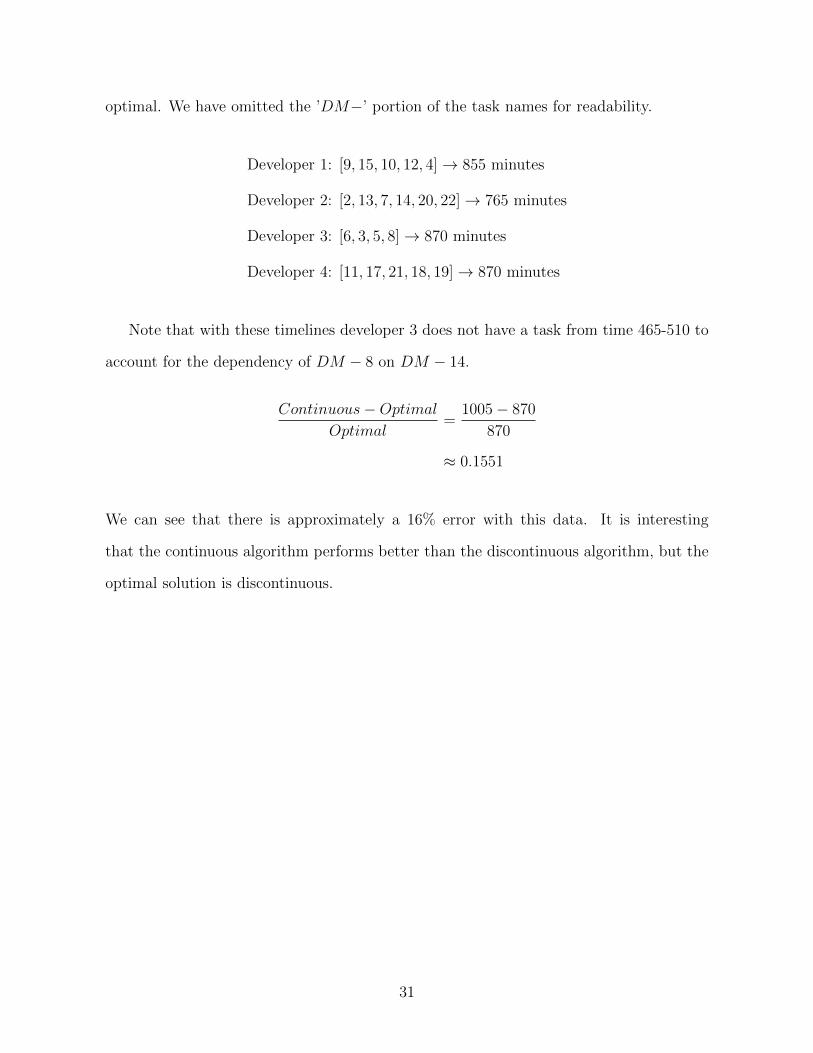
optimal. We have omitted the ’DM−’ portion of the task names for readability.
Developer 1: [9, 15, 10, 12, 4]→ 855 minutes
Developer 2: [2, 13, 7, 14, 20, 22]→ 765 minutes
Developer 3: [6, 3, 5, 8]→ 870 minutes
Developer 4: [11, 17, 21, 18, 19]→ 870 minutes
Note that with these timelines developer 3 does not have a task from time 465-510 to
account for the dependency of DM − 8 on DM − 14.
Continuous−Optimal
Optimal=
1005− 870
870
≈ 0.1551
We can see that there is approximately a 16% error with this data. It is interesting
that the continuous algorithm performs better than the discontinuous algorithm, but the
optimal solution is discontinuous.
31
5 Conclusion
This project resulted in software that could allow a project manager to get an idea
for possible timelines for a sprint. The software was built with JavaScript on a Node.js
Express server. The software was constructed with a layered structure. The kernel con-
sisted of parsing data pulled down from Jira. The next layer built all possible dependency
chains. The following layer created timelines given an unlimited amount of developers.
The final layer created timelines given a limited number of developers. The layer that
needs improvement before other layers can be developed is the limited developer layer.
Parsing data from Jira can be slightly tedious as thousands of lines of information are
pulled down with each call to the Jira API. It would be better to be able to cache the data
then only check if the sprint had been changed before making another expensive call to
the Jira API. However, once the data is parsed into nodes building dependency chains is
not too expensive relative to the general lengths of dependency chains in a given sprint. It
is almost trivial to create timelines for unlimited developers once the dependency chains
have been built, but we run into problems when creating algorithms to build timelines
with a limited number of developers.
Test data for these algorithms show that on some occasions the continuous algorithm
will perform better and other occasions the discontinuous algorithm will perform better.
However, neither of these algorithms can generally produce the optimal solution. There
is some margin of error ranging between 4% and 45%. If the margin of error is as high
as 45%, it is easy to see how to adjust the timelines by examining the placement of
independent tasks. Even though there is a large margin of error in some cases, it can
give project managers a place to start. Not only does this give managers a place to
start, a manager could run the same set of tasks through the software multiple times with
different numbers of developers, which would allow them to make swift adjustments to
32
team assignments and improve utilization.
With more time, this project could be expanded upon to include a more informative
front end. The front end could be expanded to include a display of the dependency chains
that resemble Figure 3.1, for example. From there, we could add visualizations resembling
the timelines in Figure 3.4. As mentioned, it would be ideal for this to be hosted on a web
server and be accessible to outside use. We think the best way to improve the algorithm
would be to create classifications of the overall structures of tasks in a sprint and develop
particular algorithms that would be better suited to handle those cases.
33
6 Glossary
6.1 Introduction
Definition 6.1.1. A dependency is a relationship between two tasks, such that one
task must be completed before the other task can be started.
Definition 6.1.2. A directed graph (V,E) is a graph where E is composed of order
pairs of elements of V . That is the edge (e1, e2) is distinct from the edge (e2, e1).
Definition 6.1.3. Slack is the amount of time a task can be delayed without causing a
delay in subsequent tasks or the project as a whole.
Definition 6.1.4. A story is a series of related tasks.
Definition 6.1.5. A task is a small piece of development work.
6.2 Graphs
Definition 6.2.1. A bipartite graph is a graph whose vertices can be separated into
two disjoint sets V and U such that each edge connects one vertex in V to one in U .
Definition 6.2.2. A complete graph is a graph where each pair of vertices are connected
by an edge.
Definition 6.2.3. A graph is connected if for any two vertices in a graph there is a
path between the vertices.
Definition 6.2.4. A directed graph (V,E) is a graph where E is composed of order
pairs of elements of V . That is the edge (e1, e2) is distinct from the edge (e2, e1).
Definition 6.2.5. A graph is disconnected if it is not connected.
34
Definition 6.2.6. An Eularian cycle in a graph G is a cycle that includes every edge
in G.
Definition 6.2.7. A graph G is a pair of sets (V,E) where V is nonempty, and E is a
(possibly empty) set of unordered pairs of elements of V .
Definition 6.2.8. A Hamiltonian cycle in a graph G is a cycle that contains every
vertex in G.
Definition 6.2.9. The indegree of a vertex is the number of edges going into a vertex,
a vertex with an indegree of 0 is called a root.
Definition 6.2.10. A minimum spanning tree is an edge-weighted undirected graph
that connects all the vertices together, without any cycles and with the minimum possible
total edge weight.
Definition 6.2.11. The outdegree of a vertex is the number of edges leaving a vertex,
a vertex with an outdegree of 0 is called a leaf.
Definition 6.2.12. A perfect matching is a matching of a graph such that every vertex
of the graph is incident to exactly one edge of the matching.
Definition 6.2.13. Given a directed acyclic graph G = (E, V ), a topological sort or
ordering is a linear ordering of its vertices such that for every edge (v1, v2) in G, v1 will
appear in the ordering before v2.
Definition 6.2.14. A undirected graph (V,E) is a graph where E is composed of pairs
of elements of V .
Definition 6.2.15. A graph is weighted if each branch has a numerical weight.
6.3 Design
Definition 6.3.1. An issue is the Jira term for a task, story or software bug.
35
References
[1] N. Chiba and T. Nishizeki. Planar Graphs Theory and Algorithms. Mineola, NewYork: Dover Publications Inc., 2008. isbn: 048646671.
[2] Leiseron Cormen and Rivest. Introduction to Algorithms. Cambridge, MassachusettsLondon, England: The MIT Press, 2009.
[3] D. G. Malcolm J. H. Roseboom C. E. Clark W. Fazar. “Application of a Techniquefor Research and Development Program Evaluation”. In: Operations Research (1959).doi: https://doi.org/10.1287/opre.7.5.646.
[4] Nora Hartsfield and Gerhard Ringel. Pearls in Graph Theory. Mineola, New York:Dover Publications Inc., 2003. isbn: 0486432327.
[5] Maad M. Mijwel. “Travelling Salesman Problem Mathematical Description”. In:(2016).
36
Related Documents