DEPARTMENT OF PHYSICS UNIVERSITY OF JYVÄSKYLÄ RESEARCH REPORT No. 7/2012 NUMERICAL STUDIES OF TRANSPORT IN COMPLEX MANY-PARTICLE SYSTEMS FAR FROM EQUILIBRIUM BY JANNE KAUTTONEN Academic Dissertation for the Degree of Doctor of Philosophy To be presented, by permission of the Faculty of Mathematics and Natural Sciences of the University of Jyväskylä, for public examination in FYS1 of the University of Jyväskylä on October 1, 2012 at 12 o’clock noon Jyväskylä, Finland August 2012

Welcome message from author
This document is posted to help you gain knowledge. Please leave a comment to let me know what you think about it! Share it to your friends and learn new things together.
Transcript

DEPARTMENT OF PHYSICSUNIVERSITY OF JYVÄSKYLÄ
RESEARCH REPORT No. 7/2012
NUMERICAL STUDIES OF TRANSPORT IN COMPLEXMANY-PARTICLE SYSTEMS FAR FROM EQUILIBRIUM
BYJANNE KAUTTONEN
Academic Dissertationfor the Degree of
Doctor of Philosophy
To be presented, by permission of the
Faculty of Mathematics and Natural Sciences
of the University of Jyväskylä,
for public examination in FYS1 of the
University of Jyväskylä on October 1, 2012
at 12 o’clock noon
Jyväskylä, FinlandAugust 2012

Preface
This work has been conducted during the years 2006-11 in the University of Jyväskyläat the Department of Physics. This research has provided both days with enthusiasmand the joy of discovering new, but also days with despair and frustration. However,by experiencing these both, I have learned much more during this time and I am readyfor future challenges.
I am grateful to my supervisors, Juha Merikoski for his guidance and support duringthese years, and Otto Pulkkinen for his assistance in finishing this Thesis. I also hada pleasure to work with Janne Juntunen, a past member of our small but devotedstatistical physics research group. The overall working atmosphere at the PhysicsDepartment has been pleasant.
Financial support from the Finnish Academy of Science and Letters (Väisälä fund),the Magnus Ehrnrooth Foundation, the Emil Aaltonen Foundation and the Rector ofthe University of Jyväskylä is gratefully acknowledged.
Finally I would like to thank my family and my beloved Sanni for their encouragementand support.
Jyväskylä, August 2012
Janne Kauttonen
i

Abstract
Kauttonen, JanneNumerical studies of transport in complex many-particle systems far from equilibriumJyväskylä: University of Jyväskylä, 2012(Research report/Department of Physics, University of Jyväskylä,ISSN 0075-465X; 7/2012)ISBN paper copy: 978-951-39-4786-6ISBN electronic: 978-951-39-4787-3
In this Thesis, transport in complex nonequilibrium many-particle systems is studiedusing numerical master equation approach and Monte Carlo simulations. We focuson the transport of the center-of-mass of deformable objects with internal structure.Two physical systems are studied in detail: linear polymers using the Rubinstein-Dukemodel and single-layer metal-on-metal atomic islands using a semi-empirical latticemodel. Polymers and islands are driven out of thermodynamic equilibrium by strongstatic and time-dependent external forces. Topics covered in this work include intro-ductions to nonequilibrium statistical mechanics, master equations and computationalmethods, with construction and numerical solving of master equations, and numericaloptimization. For small systems (up to ∼106 states), solving master equations numeri-cally is found to be efficient, especially when studying parameter sensitive and elusiveproperties, such as drifts caused by the ratchet effect. Speed and accuracy of themethod allows optimization with respect to continuous model parameters and transi-tion cycles, which helps in understanding the coupling between the internal dynamicsof deformable objects and their center-of-mass displacement.
Firstly, we study transport of polymers in spatially periodic time-dependent poten-tials using a standard and relaxed versions of the Rubinstein-Duke model. Two typesof potentials, flashing and traveling, are considered with stochastic and deterministictime-dependency schemes. Rich non-linear behavior for the transport velocity, diffu-sion and energetic efficiency is found. By varying the polymer length, we find currentinversions caused by a ’rebound’ effect that is only present for objects with internalstructure. These results are different between reptating and non-reptating polymers.Transport is found to become more coherent for deterministic time-dependency schemeand as the polymer gets longer. The results show that small changes in the moleculestructure (e.g. the charge configuration) and the environment variables can lead to alarge change in the velocity.
Secondly, we study transport of single-layer metal-on-metal islands using a semi-empirical lattice model for Cu atoms on Cu(001) surface. Two types of time-dependentdriving are considered: a pulsed rotated field and an alternating field with a zero av-erage force (an electrophoretic ratchet). The main results are that a pulsed field canincrease the velocity in both diagonal and axis directions as compared to a static
ii

Abstract iii
field, and there exists a current inversion in an electrophoretic ratchet. In additionto a ’magic size’ effect for islands in equilibrium, a stronger odd-even effect is foundin the presence of large fields. Master equation computations reveal nonmonotonousbehavior of the leading relaxation constant and effective Arrhenius parameters. Op-timized transition cycles shed light on microscopic mechanisms responsible for islandtransport in strong fields.

Author’s address Janne KauttonenDepartment of PhysicsUniversity of JyväskyläFinland
Supervisors Docent Juha MerikoskiDepartment of PhysicsUniversity of JyväskyläFinland
Doctor Otto PulkkinenDepartment of PhysicsTampere University of TechnologyFinland
Reviewers Doctor Jan ÅströmCSC - IT Center for Science Ltd.Finland
Professor Mikko KarttunenDepartment of ChemistryUniversity of WaterlooCanada
Opponent Professor Joachim KrugInstitute for Theoretical PhysicsUniversity of CologneGermany
iv

List of Publications
The main results of this Thesis have been reported in the following articles:
I J. Kauttonen, J. Merikoski, and O. Pulkkinen: Polymer dynamics in time-dependent periodic potentials, Phys. Rev. E 77, 061131 (2008).doi:10.1103/PhysRevE.77.061131.
II J. Kauttonen and J. Merikoski: Characteristics of the polymer transport inratchet systems, Phys. Rev. E 81, 041112 (2010).doi:10.1103/PhysRevE.81.041112.
III J. Kauttonen and J. Merikoski: Single-layer metal-on-metal islands driven bystrong time-dependent forces, Phys. Rev. E 85, 011107 (2012). A separate sup-plemental material to this article is available on the corresponding website ofthe article. doi:10.1103/PhysRevE.85.011107
The Author of this Thesis has done all theoretical and numerical computations, andperformed all data analysis. He has written the first versions of all the articles.
v

Contents
1 Introduction 1
2 Theory 32.1 Statistical mechanics . . . . . . . . . . . . . . . . . . . . . . . . . . . . 3
2.1.1 Systems in and out of equilibrium . . . . . . . . . . . . . . . . . 32.1.2 Linear response theory . . . . . . . . . . . . . . . . . . . . . . . 42.1.3 Graph representation . . . . . . . . . . . . . . . . . . . . . . . . 52.1.4 The ratchet effect . . . . . . . . . . . . . . . . . . . . . . . . . . 6
2.2 The Master equation . . . . . . . . . . . . . . . . . . . . . . . . . . . . 82.2.1 Derivation . . . . . . . . . . . . . . . . . . . . . . . . . . . . . . 82.2.2 Transition rates . . . . . . . . . . . . . . . . . . . . . . . . . . . 112.2.3 Properties and representations . . . . . . . . . . . . . . . . . . . 12
3 Models 193.1 External potentials . . . . . . . . . . . . . . . . . . . . . . . . . . . . . 19
3.1.1 Deterministically time-dependent potentials . . . . . . . . . . . 203.1.2 Stochastically time-dependent potentials . . . . . . . . . . . . . 203.1.3 Simple limits of the temporal period . . . . . . . . . . . . . . . 21
3.2 Observables . . . . . . . . . . . . . . . . . . . . . . . . . . . . . . . . . 233.2.1 Velocity and diffusion coefficient . . . . . . . . . . . . . . . . . . 233.2.2 Energetic efficiency . . . . . . . . . . . . . . . . . . . . . . . . . 243.2.3 Shape deformations . . . . . . . . . . . . . . . . . . . . . . . . . 253.2.4 Relaxation time . . . . . . . . . . . . . . . . . . . . . . . . . . . 26
3.3 The Rubinstein-Duke model . . . . . . . . . . . . . . . . . . . . . . . . 263.3.1 The stochastic generator . . . . . . . . . . . . . . . . . . . . . . 273.3.2 Observables of interest . . . . . . . . . . . . . . . . . . . . . . . 293.3.3 Non-uniform charge distributions . . . . . . . . . . . . . . . . . 30
3.4 The model for single-layer metal islands . . . . . . . . . . . . . . . . . . 313.4.1 The stochastic generator . . . . . . . . . . . . . . . . . . . . . . 313.4.2 The reduced model . . . . . . . . . . . . . . . . . . . . . . . . . 343.4.3 Observables of interest . . . . . . . . . . . . . . . . . . . . . . . 35
4 Setting up the equations 374.1 Constructing the master equation sets . . . . . . . . . . . . . . . . . . 37
4.1.1 Recursive method for the repton model . . . . . . . . . . . . . . 384.1.2 Enumeration method for the island model . . . . . . . . . . . . 45
4.2 Expected values of path-dependent observables . . . . . . . . . . . . . . 49
vi

Contents vii
4.2.1 Direct method . . . . . . . . . . . . . . . . . . . . . . . . . . . . 504.2.2 Generating function method . . . . . . . . . . . . . . . . . . . . 51
5 Computational methods 555.1 Numerical linear algebra and integration methods . . . . . . . . . . . . 57
5.1.1 Solving eigenstates and linear problems . . . . . . . . . . . . . . 575.1.2 Numerical integration . . . . . . . . . . . . . . . . . . . . . . . . 63
5.2 Optimization . . . . . . . . . . . . . . . . . . . . . . . . . . . . . . . . 675.2.1 Optimization with respect to cycles . . . . . . . . . . . . . . . . 675.2.2 Optimization with respect to continuous parameters . . . . . . . 72
5.3 Monte Carlo method . . . . . . . . . . . . . . . . . . . . . . . . . . . . 78
6 Results for the repton model 816.1 Choosing the rates . . . . . . . . . . . . . . . . . . . . . . . . . . . . . 826.2 Relaxation in a flashing ratchet . . . . . . . . . . . . . . . . . . . . . . 826.3 Velocity and diffusion in the steady state . . . . . . . . . . . . . . . . . 87
6.3.1 Flashing ratchet . . . . . . . . . . . . . . . . . . . . . . . . . . . 876.3.2 Traveling potential . . . . . . . . . . . . . . . . . . . . . . . . . 89
6.4 Non-uniform charge distributions . . . . . . . . . . . . . . . . . . . . . 926.5 Efficiency of the transport in a flashing ratchet . . . . . . . . . . . . . . 946.6 Time-evolution of observables . . . . . . . . . . . . . . . . . . . . . . . 976.7 Transition sequences . . . . . . . . . . . . . . . . . . . . . . . . . . . . 1006.8 Discussion . . . . . . . . . . . . . . . . . . . . . . . . . . . . . . . . . . 103
7 Results for the island model 1057.1 Pulsed field and electrophoretic ratchet . . . . . . . . . . . . . . . . . . 1067.2 Static field . . . . . . . . . . . . . . . . . . . . . . . . . . . . . . . . . . 107
7.2.1 Velocity as a function of field . . . . . . . . . . . . . . . . . . . 1077.2.2 The effect of the measuring and field angles . . . . . . . . . . . 1107.2.3 Energy barriers and the leading relaxation constant . . . . . . . 112
7.3 Time-dependent field . . . . . . . . . . . . . . . . . . . . . . . . . . . . 1157.3.1 Pulsed field . . . . . . . . . . . . . . . . . . . . . . . . . . . . . 1157.3.2 Electrophoretic ratchet . . . . . . . . . . . . . . . . . . . . . . . 116
7.4 Transition sequences . . . . . . . . . . . . . . . . . . . . . . . . . . . . 1207.5 Discussion . . . . . . . . . . . . . . . . . . . . . . . . . . . . . . . . . . 122
8 Summary 126
Appendices 129
A Time-dependent DMRG 129
B Derivation of equations (4.2) and (4.3) 133
Bibliography 136

1 Introduction
Research of transport of complex molecular and micro-scale objects has flourished inthe last two decades. Important discoveries have been made and knowledge has beengained on molecular motors, polymers and in surface physics, where the developmentin experimental and computational techniques have reached the level which allowsstudying and manipulation of individual molecules and atoms [85, 34, 33]. Theoret-ical research of simplified models has a center stage in unraveling the operationalprinciples of these systems. In this work two complex micro-scale systems are studied:linear polymers and single-layer atomic islands [5, 86, 110, 139]. We apply a masterequation approach and simulations, and concentrate on the transport properties ofpolymers and islands under the effect of strong static and time-dependent externalforces. Topics covered in this work include introductions to nonequilibrium statisti-cal mechanics, master equations and computational methods, with construction andnumerical solving of master equations, and numerical optimization.
Statistical mechanics consists of two rather different parts: equilibrium and nonequi-librium statistical mechanics. A system is said to be in thermodynamic equilibriumwhen it is thermally, mechanically, radiatively and chemically in balance, i.e. there areno net flows of matter or energy, no phase changes, and no unbalanced potentials ordriving forces, within the system [27]. An equilibrium system experiences no changeswhen it is isolated from its surroundings. If any of these conditions is not met, thesystem is in a nonequilibrium state [75].
The success of equilibrium statistical mechanics has been spectacular. It has beendeveloped to a high degree of mathematical sophistication, and applied with suc-cess to subtle physical problems like the study of critical phenomena. By contrast,the progress of nonequilibrium statistical mechanics has been much slower. For sys-tems in equilibrium, everything is well understood and validated, but as the systemsand processes of interest are taken further from thermodynamic equilibrium, theirstudy becomes much more difficult. We still depend on the insights of Boltzmannfor our basic understanding of irreversibility, and further progress has been mostlyon dissipative phenomena close to equilibrium, resulting in Onsager reciprocity rela-tions, Green-Kubo formula, and related fundamental results [75, 27, 138]. Theory ofnonequilibrium systems is still immature and under development. Indeed, developinga fundamental and comprehensive understanding of physics far from equilibrium isrecognized to be one of the ’grand challenges’ of our time, by both the US NationalAcademy of Sciences and the US Department of Energy [33, 201]. Perhaps the most
1

2 Introduction
striking feature of nonequilibrium systems is the possibility for mass transport. Trans-port near equilibrium is covered by the linear response theory and is generally wellunderstood. On the other hand, far from equilibrium, complex and strongly system-dependent, non-linear transport phenomena arise. The motivation behind this workis to gain understanding about these phenomena.
The master equation approach is an efficient way to study the statistical mechanics ofcomplex nonequilibrium many-particle systems. In this work, we concentrate on thenumerical methods for large master equation sets and provide in-depth analyses ofdiscrete state polymer and single-layer metal island models in nonequilibrium condi-tions. Both polymers and atomic islands have large numbers of internal configurations.Our main focus lies on the transport properties of these deformable objects, whichare very different from objects without internal structure, such as point-like particles.Nonequilibrium state is obtained by introducing strong static and time-dependentpotentials that force the system out of equilibrium.
In the first part of this work, we concentrate on the numerical solution methods ofmaster equations. If the number of master equations is of order 106 or less, numeri-cally exact results for the probability distribution and observables of nonequilibriummodels can be computed. As opposed to the Monte Carlo simulations, which is thetraditional numerical method, speed and accuracy of the numerical master equationmethod allows numerical optimization with respect to continuous model parametersand transition cycles. This helps in understanding the coupling between the inter-nal dynamics of deformable objects and their center-of-mass displacement. Numericalmaster equation approach has been previously used mostly in studies of chemical re-action networks (e.g. stoichiometry) and related fields [63]. In this work, we show thatthis method can be also used as a standard tool in studies of complex many-particlesystems in nonequilibrium statistical physics. This has became possible mainly dueto the recent advances in computer technology and numerical methods, particularlyin linear algebra and optimization. In this Thesis, we will cover all necessary theoreti-cal and numerical aspects of the master equation method for nonequilibrium discretemodels.
The Thesis is organized as follows. In Chapter 2, the theoretical basis of nonequilib-rium systems, the ratchet effect and master equations are presented. The presentationis kept general without making assumptions of any specific models. In Chapter 3 wepresent and define the models and observables studied in this work. In Chapters 4and 5, methods to set up and solve master equations are discussed. In Chapters 6and 7, results for the repton and island model are presented and discussed. Finally,in Chapter 8, the summary and outlook of this Thesis is presented.

2 Theory
In this Chapter, the general theoretical background of the Thesis is presented. To keepthe representation compact and readable, many mathematical details are omitted. Weconcentrate on systems with a finite discrete set of states, with brief exceptions madein Sections 2.1.4 and 2.2.1.
2.1 Statistical mechanics
2.1.1 Systems in and out of equilibrium
The fundamental property of the equilibrium is that the probability to find the systemin a given state follows the Boltzmann distribution [138]
Peq(y) =1
Ze
−E(y)kBT , (2.1)
where y denotes the microstate of the system with energy E(y), kB is the Boltzmannconstant, T is the temperature and Z =
∑y exp (−E(y)/kBT ) is the partition function
over all available microstates in the canonical ensemble. The second requirement forthermodynamic equilibrium is the local detailed balance condition [138]
Peq(y)W (y′, y) = Peq(y′)W (y, y′), (2.2)
where W (y′, y) is the transition rate (probability per unit time) for a transition fromstate y to state y′. The products of the form P (y)W (y, y′) are called probability flowsor currents. Together with the distribution P , these flows have a special role in charac-terizing the steady states uniquely [200]. For discrete time systems, W is the transitionprobability (see Section 2.2.3 for more details). The detailed balance condition is avery strong property, because it indicates that there cannot be net currents betweenany states in the system, and if W (y, y′) is non-zero, then also W (y′, y) must be non-zero. From the detailed balance condition, it also follows that the dynamics of theequilibrium system is independent of the direction of time and the entropy produc-tion of the system is zero.
For a nonequilibrium system, equations (2.1) and (2.2) do not hold. There is no generalparadigmatic theoretical framework that describes nonequilibrium systems, neither in
3

4 Theory
thermodynamics nor in statistical mechanics [75, 194]. Especially, this means thatthere is no general principle whereby one can calculate the distribution of the sys-tem’s states from the sole knowledge of the system’s invariants or external constraintsimposed on the system. At present, the most promising results in the search for uni-versal properties of nonequilibrium systems are the fluctuation and pumping theorems[76, 29, 8]. These theories go beyond linear response regime (see below), but the prac-tical usefulness of these expansions remains an open question. They provide certainlimits and requirements for the work and current distributions, but do not provide anactual access to their distributions [8]. Numerical methods remain the main tool tostudy complex systems far from equilibrium.
In this work, we only consider ergodic (irreducible) systems, which means that thesystem has a non-zero probability to visit all microstates regardless of the initialstate. If this is not true, then the system consists of disconnected sub-systems (thesystem is decomposable) and each sub-system can be treated as separately from eachother. Any ergodic system finally relaxes to an unique steady state corresponding toa function W if allowed to run infinitely long. For equilibrium systems, W must betime-independent and lead to the Boltzmann distribution with the detailed balance[138]. A nonequilibrium state can be steady or transient. A transient nonequilibriumstate appears, for example, after the system is suddenly pushed out of equilibrium. Ifthe system is pushed out of equilibrium with periodic or constant forces, the systemwill end up in a nonequilibrium steady state. In this work, we mainly concentrate onthe latter type of nonequilibrium systems.
2.1.2 Linear response theory
It is known empirically, that for a large class of irreversible phenomena and under awide range of experimental conditions, irreversible flows are linear functions of thermo-dynamic forces [120, 27]. Majority of studies and theory of nonequilibrium statisticalmechanics are limited within the linear response regime near the equilibrium. Whenthermodynamic forces are introduced in a system in thermodynamic equilibrium, ir-reversible dynamics with currents appear. If the forces are small, the response of thesystem can be linearized such that
Xi =∑
j
Li,jFj,
where Fj are the thermodynamic forces and Xi are the resulting currents. The co-efficients Li,j are called Onsager kinetic coefficients. Positive definiteness of entropyproduction requires that Li,i ≥ 0 and by the local detailed balance condition, one getsOnsager’s principle Li,j = Lj,i ≥ 0 [107]. Many well-known relations, such as Ohm’s,Fourier’s and Fick’s laws, indeed rely on the linear response. The cornerstone of the

2.1 Statistical mechanics 5
linear response theory is the fluctuation-dissipation theorem, which states a generalrelationship between the response of a given system to an external disturbance andthe internal fluctuation of the system in the absence of the disturbance. Perhaps thebest known example of the fluctuation-dissipation theorem is the Einstein relation
D = µkBT,
where D is the diffusion coefficient at equilibrium and µ = v/F is the mobility, whichis the drift velocity of the object, divided by the total force F affecting the system.This means, that v ∝ D for small forces, i.e. the equilibrium diffusion coefficient canbe determined from nonequilibrium currents near equilibrium, which is often mucheasier than trying to evaluate D directly. By checking the linearity of the drift, one canalso get an idea of how close to equilibrium the system is. The fluctuation-dissipationtheorem is useful because it gives a relation between two quantities related to twoessentially different processes, e.g. drift and fluctuations.
2.1.3 Graph representation
The function W in Eq. (2.2), which consist of allowed transitions between microstates,can be also understood as a graph: If W (i, j) > 0, there is a connection (edge) betweenstates (vertices) i and j. The process defined by W then becomes equivalent to arandom walk on a graph [16, 117, 95]. The topology and the complexity of the graphdepends on the details of the system. A time-dependent set of vertices connected byedges is called a path and its time-independent counterpart a sequence. For an ergodicsystem, the graph consists of a single strongly connected component, i.e. there existsa sequence between any two vertices in the graph. Sequences with the same startingand ending vertices are called cycles, and they have a special importance in the theoryof nonequilibrium systems. For equilibrium systems, it follows from Eq. (2.2) that forevery cycle C one has ∏
〈i,j〉∈C
W (i, j)
W (j, i)= 1,
where 〈i, j〉 is a directed edge in the configuration graph. A system with this prop-erty is said to have a balanced dynamics. This condition does not generally result inEq. (2.2). For non-equilibrium systems, the right-hand side of the above equation isreplaced by exp(A(C)) for some cycles, where the affinity (or a macroscopic force)A(C) of the cycle measures the deviation from equilibrium and is generally non-zero.Cycles with non-zero affinities are sometimes called ’irreversible rate loops’. In hisseminal paper in 1970s, Schnakenberg formulated a theory of macroscopic observ-ables as circulations of local forces, and identified the total entropy production of athermodynamic system using cycles and their affinities [165]. It is currently unclear,whether there exists an intuitively accessible and simple relationship between current

6 Theory
circulations and non-zero affinities [33]. It has been found, that circulations give riseto the stochastic resonance effect [142]. One of the major differences between equilib-rium and nonequilibrium systems is, that, for an equilibrium system, the steady statedistribution Peq does not depend on the topology of the graph, i.e. for an ergodicsystem, the distribution remains the same for different placements of edges betweenvertices. However, for transport properties, the topology of the graph is important forboth kind of systems.
2.1.4 The ratchet effect
The properties of nonequilibrium systems depend on how they are driven out of equi-librium. In this work we are especially interested in systems under thermal randommotion with the presence of time-dependent forces, whose time-averaged force remainszero, but yet there exists net transport of mass. The transport arises as a subtle inter-play between nonlinearities in the system and broken symmetries. This type of noiseinduced transport is generally known as a ratchet effect [148] and it is different fromthe usual predictable mechanical transport, that follows directly from the gradientsof the forces. Due to fluctuations, the time-evolution of state variables, such as theposition of an object, are not directly coupled to the time-evolution of potentials, andlarge deviations from an average trajectory can occur. State variables of microscopicsystems in noisy environment are therefore said to be loosely coupled with potentials,whereas a macroscopic apparatus always displays tight coupling.
For biological systems, ratchet effect poses one of the mechanisms how they manageto keep themselves in ordered states even while surrounded by significant thermalnoise and environmental fluctuations. In the inorganic and macroscopic world, trans-port always take place along a gradient of the potential, such as gravitation, electricfield, chemical imbalance and temperature differences. This is not how transport isachieved for most biological systems. For example, thermal gradients are essentiallyimpossible to maintain over small distances, hence the thermal gradients necessary todrive significant motion are not realistic. With the ratchet effect, directed motion ispossible without long-range gradients [11, 85, 4, 182].
The ratchet effect discussed here takes place when the following conditions are met:(1) the system is spatially periodic, (2) there is some asymmetry in the potentials, and(3) the system is out of equilibrium. We will next distinguish between the main typesof ratchets. For this, it is more convenient to consider a single overdamped1 Brownianparticle in a periodic one-dimensional potential V (x+ L, t) = V (x, t), where L is thespatial period of the potential. The main classification of ratchets remains the same
1For overdamped particles the effect of inertia is neglected, i.e. an approximation x(t) ≈ 0 isapplied.

2.1 Statistical mechanics 7
for discrete systems and non-Gaussian noises. The equation of motion for a Brownianparticle, also known as the Langevin equation, in a medium is
ηx = − d
dxV (x, t) + F + y(t) + ε(t),
where η is a friction coefficient, F is a constant load-force, y(t) is a time-dependentforce and ε(t) is a random motion (noise). The most studied and familiar type ofnoise is the Gaussian one (i.e. white noise), for which 〈ε(t)ε(s)〉 = 2ηkBTδ(s− t) and2ηkBT = D is identified as a diffusion coefficient.2 The potential V is expected tooriginate from the medium, whereas F and y result from external fields.
Based on the choice of V , two distinct types of ratchets can be defined: fluctuatingpotential ratchet with V (x, t) = V (x) [1 +W (t)] and traveling potential ratchet withV (x, t) = V (x −W (t)). In the first one, the amplitude of the potential and in thesecond one the location fluctuates. For the first type, two especially interesting andwidely used potential types can be identified:
• On-off ratchet: V (x, t) ∈ V (x), 0, F = y(t) = 0.
• Rocking ratchet: V (x, t) = V (x) and 〈F + y(t)〉t = 0
The ratchet effect occurs when d〈x〉/dt 6= 0 for 〈−dV (x, t)/dx+F+y(t)〉 = 0, i.e. thereis a net drift in the presence of a vanishing mean force.
For the ratchet effect to take place, the magnitude of potentials V , y and F aretypically of same magnitude as the thermal energy kBT . For zero temperature, theratchet effect vanishes. Current inversions, which means that the transport directionturns around, are found to be rather common and can usually be generated by particleinteractions and tuning of variables (e.g. diffusion constant, friction, potential shapeand period) [148, 106, 196, 32, 38, 31, 26, 109, 100]. Since the systems utilizing theratchet effect work under nonequilibrium conditions, they are exactly solvable only insimplest cases. Some exact results can, however, be often derived at different limits,such as very small/large potentials and slowly/fast changing potentials, for which theresults from the equilibrium statistical mechanics can be utilized in some form.
The first major contribution towards the studies of the ratchet effect was by Smolu-chowski in his Gedankenexperiment in 1912, regarding to the absence of directedtransport in a system consisting only a single heat bath [174]. The next importantstep was taken by Feynman using the famous ’ratchet and pawl’ model, for which thequantitative analysis was published in 1962 and which showed, that that external workis required for the machine to perform useful work [62].3 However, it was the works by
2For this reason, the term Brownian motor is often used for objects that utilize the ratchet effect.3See Ref. [89] for an exactly solvable discrete counterpart of the ’ratchet and pawl’ model.
8 Theory
Ajdari, Prost, Magnasco et al. in early 1990’s, that provided the inspiration for a wholenew wave of great theoretical and experimental activity, and progress within the sta-tistical physics community [141, 118]. Another root of Brownian motor theory originsfrom the intracellular transport research, specifically the biochemistry of molecularmotors and molecular pumps [186]. Most studies, especially the theoretical ones, haveconcentrated on one dimensional systems and white thermal noise. More recently, two-dimensional systems, complicated potentials, colored noises and non-point-like objectshave been considered [54, 97, 68, 121, 140, 22, 14, 169, 190, 59, 187, 60, 149, 187]. Theratchet effect has been also studied in other contexts, such as the game theory, wherethe so-called Parrondo’s paradox is a discrete counterpart to the Brownian particleversion [133].
2.2 The Master equation
In this section we derive, motivate and discuss properties of master equations whichform the mathematical framework of this work. Master equations describe the time-evolution of a system, that can be modeled as being in exactly one of countable numberof states at any given time, such that the switching between the states is treatedprobabilistically. A system governed by the master equations can be interpreted asrandom walks and are therefore often called jump processes.
Despite the simplicity of the master equation, it has been a subject for decades oftheoretical research and countless applications. Typical examples of usage in physicsare lattice models (e.g. simple exclusion and zero-range processes) and Fermi-Goldenrule in quantum mechanics. Theoretical research of nonequilibrium systems have beenmostly done within the context of master equations, resulting in e.g. fluctuation andpumping theorems. A large portion of theoretical and numerical research of masterequations have been done particularly in the area of chemistry, where they are used tomodel chemical reactions (e.g. reaction networks). The popularity of master equationsis also explained by their close relation to the Fokker-Planck equation and differenttypes of random walks, in both discrete and continuous space and time.4
2.2.1 Derivation
In the following, a derivation of master equations is given, starting from a genericrandom process. More comprehensive and mathematically rigorous derivations can be
4For example, the Fokker-Planck equation gives the distribution for a particle governed by theLangevin equation [152]. On the other hand, these two can be recovered from the appropriate discreterandom walks at the limit of infinitesimal spatial and/or temporal steps.

2.2 The Master equation 9
found in several textbooks such as [129, 73, 66].
Consider a stochastic process Y (t) in continuous time and space. According to theBayes’ rule, the following identity holds for the joint probability:
P (y1, t1; y2, t2) = P (y1, t1)P (y2, t2|y1, t1),
where P (y2, t2|y1, t1) is the conditional probability and yi := Y (ti). Now, if for allsuccessive times t1 < t2 < · · · < tn the condition
P (y1, t1; y2, t2; . . . ; yn, tn) = P (y1, t1)P (y2, t2; . . . ; yn, tn|y1, t1)= P (y1, t1)P (yn, tn|yn−1, tn−1) . . . P (y2, t2|y1, t1),
holds, then the process Y (t) is called a Markov process. Such process is completelydetermined if one knows P (y, t) and P (y2, t2|y1, t1), i.e. the probability to be in thegiven state in a given time, and the probability for a transition to another state fromthe previous [177]. The future state of the process depends only on the present stateand not on the past history. For the case n = 3 and integrating the equation above,one receives the identity
P (y3, t3; y1, t1) =
∫P (y3, t3|y2, t2)P (y2, t2|y1, t1)dy2, (2.3)
which is known as the Chapman-Kolmogorov equation for Markov processes. A Markovprocess is fully determined by P (y, t) and P (y2, t2|y1, t1), but these functions cannot bechosen arbitrarily. Two properties are required: Non-negative and properly normalizedfunctions P (y, t) and P (y2, t2|y1, t1) satisfying Eq. (2.3) and
P (y2, t2) =
∫P (y1, t1)P (y2, t2|y1, t1)dy1
uniquely define a Markov process.
The conditional transition probability can be expanded in time such that
P (y2, t1 + δt|y1, t1) = δ(y1 − y2) [1− A(y1)δt] + δtH(y2|y1) +O(δt2), (2.4)
where H(y2, y1) ≥ 0 is the transition probability per unit time from y1 to y2. Thecoefficient 1 − A(y1)δt is the probability that no transition takes place during δt.Normalization requires that
A(y1) =
∫H(y2|y1)dy1.
Substituting this into (2.3) and taking the limit δt → 0 leads to the differential formof the Chapman-Kolmogorov equation,
dP (y, t|y0, t0)dt
=
∫[H(y|y′)P (y′, t′|y0, t0)−H(y′|y)P (y, t|y0, t0)] dy′,

10 Theory
which is known as the master equation. For a system with a discrete state space,which is the case considered in this work, master equations have a form
dPy(t)
dt=∑
y′ 6=y
[Hy,y′Py′(t)−Hy′,yPy(t)] , (2.5)
where the function H includes all states of the system with Hy′,y > 0 for allowedtransitions between states and zero to others. This type of a process is also called as acontinuous-time Markov chain. The expected transition time from state y to state y′
is given by 1/Hy′,y. Therefore, the average lifetime of state y is simply 1/∑
y′ 6=yHy′,y.Alternatively, master equations can be written in the form
dPy(t)
dt=∑
y′ 6=y
[Jy,y′(t)− Jy′,y(t)] ,
where Jy,y′(t) := Hy,y′Py′(t) is the probability flow from state y′ to state y.
Because H creates the dynamics for the process, it is called a stochastic generatorof the Markov chain. Particularly in physics, it is also known as a Liouville oper-ator or a stochastic Hamiltonian. Although the underlying process is random, thetime-evolution of the probability is deterministic. Random realizations (paths) of theprocess can be sampled with Monte Carlo methods, whereas the probability distribu-tion can be numerically computed with differential equation solvers. These methodsare discussed in detail in Chapter 5.
Finally we note that, from the Markov property, it follows that the waiting time distri-butions of jumps are exponentially distributed. This can be also seen by starting fromthe so called generalized master equation, which includes arbitrary time-dependentmemory kernels. By assuming exponential waiting times, the memory kernels thenreduces to constants, which are identified as rates Hy,y′ , leading to Eq. (2.5). SeeRefs. [96, 57] for additional details of this connection.
————
As an example, at the end of this subsection, let us consider a homogeneous continuous-time random walk on one-dimensional infinite lattice. At time t = 0, the randomwalker is at the origin, i.e. n(t = 0) = 0, and the walker moves to left or rightneighbor lattice site with a finite rate γ > 0. Master equation for this process is
dPn(t)
dt= γPn−1(t) + γPn+1(t)− 2γPn(t),
where Pn(t) is the probability for n(t). To solve this, we note that since jump timesand directions are clearly two independent processes, the solution of this process has

2.2 The Master equation 11
the form
Pn(t) =∞∑
i=0
Pi(t)Pi(n),
where Pi(t) is the probability for i events until time t and Pi(n) is the probabilityto end up at point n with i jumps. The first is the Poisson distribution, while thelatter is given by the Bernoulli distribution shifted to the origin. Plugging them in,the complete solution reads
Pn(t) =∞∑
i=0
(γt)i exp(−tγ)n!
1
2ii!(
i−n2
)!(i+n2
)!= exp(−tγ)In(γt),
where In(γt) is a modified Bessel function. For large spatial and temporal scales, thisprocess is analogous to Brownian motion on real axis. For more than one rate, theproblem becomes much more complicated, since the above two processes are no longerseparable. The models studied in this work (see Sections 3.3 and 3.4) can be viewed asextensions of this simple model, with much more complicated state-space with non-homogeneous and time-dependent rates, hence only the numerical solution methodscan be applied.
2.2.2 Transition rates
The master equation is only useful if one knows the transition rates of the process. Fora physical model, there are basically two ways to get them. The first way is to calculatethem from some ’microscopic’ model. The other is to derive them from experimentalor simulation data. If master equations are used to model a thermodynamic system,the elements of H must be chosen such that the equilibrium conditions (2.1), (2.2)and ergodicity, discussed in Section 2.1, are fulfilled. There is no guarantee that theseconditions are fulfilled if the rates are taken directly from an experiment or some mi-croscopic simulation. In this work, we only consider models for which these conditionshold.
Conditions (2.1) and (2.2) do not specify the transition rates uniquely, but only theirratios. Despite the large number of studies with discrete nonequilibrium models, theimportance of choosing the rates Hi,j has not got much attention. However, this choicebecomes very important when studying transport in complicated potentials. The usualchoices for the rates are [84, 92]
Hi,j/Γ =
min1, e(Ej−Ei)/kBT
(Metropolis)
e(Ej−Ei)/2kBT (exponential)[1 + e(Ei−Ej)/kBT
]−1(Kawasaki),

12 Theory
where the constant Γ > 0 sets the time-scale. All three definitions lead to Boltzmanndistribution in equilibrium and fulfill local detailed balance (2.2), but generate thedifferent kinds of dynamics.
Being fast and simple, the Metropolis form is usually the first choice for the rates.Especially when studying the ratchet effect, it can be a poor choice since it does nottake into account the slope of the downhill moves (rate being limited to Γ), that canbe important for the dynamics. This is also the case for the Kawasaki form, sinceit is basically just a smoothened Metropolis function. Differences between the abovethree rate types are demonstrated in Section 6.1 for the repton model. The selectionof suitable rates must be made on experimental or other system-specific grounds.
2.2.3 Properties and representations
In this Section we consider some important general properties of the master equationset. As noted before, we consider only systems with a finite number of states.5
Matrix form and eigenstates
Setting Hy,y = −∑y′ Hy′,y, master equations of the form (2.5) can be written in acompact matrix form
dP (t)
dt= H(t)P (t), (2.6)
where the probabilities of states are given by components of vector P (t). In the liter-ature, matrix H is sometimes called a Q-matrix. It has following properties:
• If H is nonsymmetric, its left and right eigenvector sets 〈ψi| and |ϕi〉 are dif-ferent but have the same eigenvalues λi. Eigenvector sets are non-orthogonal,i.e. 〈ϕi|ϕj〉 6= 0 for i 6= j (and similarly for 〈ψi|), but create a bi-orthogonal set〈ψi|ϕj〉 = 0 for all i 6= j.
• H is negative semidefinite, i.e. its eigenvalues are less than or equal to zero.
• There exists at least one eigenstate with an eigenvalue zero. If H is irreducible,there is exactly one eigenstate corresponding to eigenvalue zero, meaning thatthe steady state is unique.
• Non-zero eigenvalues can contain an imaginary part, in which case they comein complex-conjugate pairs.
5Many of the properties covered in this Section also hold for countably infinite number of states,but then many mathematical complications related to uniqueness and normalization arise.

2.2 The Master equation 13
The right eigenstate corresponding to the eigenvalue zero is the most important one,since it is the steady state solution of time-independent H. The steady state is a time-homogeneous probability distribution which describes the system in the long-timelimit. The corresponding left eigenstate can be used to compute expected values ofobservables (see below).
Above properties essentially follow from elementary linear algebra and the followingform of the Perron-Frobenius theorem: If a square matrix A is non-negative andirreducible, then
1. A has a positive real eigenvalue λ which is equal to its spectral radius, i.e. λ =maxk |λk(A)|, where λk(A) denotes the kth eigenvalue of A.
2. λ corresponds to an eigenvector with all its entries being real and positive.
3. λ is a simple eigenvalue of A.
This theorem applies to H through its time-development operator (discussed later)with the properties given above [94, 65].
The non-symmetry property of H turns out to be problematic for both theoreticaland numerical analysis [69]. This is especially true in the absence of detailed balance.6
Complex eigenvalues result in oscillations in time-dependent states and can be relatedto the stochastic resonance effect [142, 143]. Since the columns of the matrix H sumto zero, the rank of the matrix is always one less than the dimension of the matrix,i.e. the matrix H is singular. However, this poses no problem, since we also havenormalization conditions, which ensures the uniqueness of the linear and eigenvalueproblems related to H.7
The matrix H has right and left vectors corresponding to the same eigenvalues,i.e. H|ϕy〉 = λy|ϕy〉 and 〈ψy|H = 〈ψy|λy. Using normalization 〈ψi|ϕj〉 = δi,j, the
formal solution of (2.6) is given by |P (t)〉 = exp(∫ t
s=0H(s)ds
)|P (0)〉, where |P (0)〉
is the initial state. This time-dependent state |P (t)〉 is a transient state. For a time-independent H, this can be expressed using the eigenvectors
|P (t)〉 =∑
y
〈ψy|P (0)〉eλyt|ϕy〉,
which is known as the eigenfunction expansion.
6With detailed balance, the matrix H can be diagonalized using the equilibrium steady state P eq
with a transformed symmetric matrix Hi,j =(P eqj /P eq
i
)1/2Hi,j
7For example, when solving problems Hx = 0 and Hx = b, one can replace one row of H withones and use normalization conditions.

14 Theory
If an observable of interest can be put into a matrix form, i.e. it only depends on theprobability distribution, its expected value can be computed using
〈O(t)〉 =∑
i
OiPi(t) = 〈ψ0|O|P (t)〉, (2.7)
where O is the operator of the observable and 〈ψ0| is the left eigenstate correspondingto the eigenvalue zero such that 〈ψ0|P (t)〉 = 1 holds. To compute long-time averages,the steady state distribution for |P (t)〉 is used, which is either time-independent orperiodic in time. Note that, if the chosen basis is the natural basis, which is usually thebest choice, the operator O is a diagonal matrix and one can also compute 〈O(t)〉 =Tr(OP (t)). Similarly, the variance 〈O〉2 − 〈O2〉 describing the fluctuation, can becomputed using the operator with squared elements.
Operator formalism
For some stochastic systems, H can be naturally build with local operators. For suchoperator formalism to be efficient, a compact, fixed lattice representation is required.By compactness, we mean that the matrix H is irreducible, hence there are no emptyrows or columns corresponding to null states when using the natural basis.8 In physics,such models are often one or two dimensional simple models of particle motion. Typicalexamples are simple exclusion processes (1D), zero-range processes (1D), Hubbardmodel (1D) and Ising model (1D and 2D). In the operator formalism, the stochasticgenerator has a general form
H =∑
I∈L
[E(I)−D(I)] ,
where the index set I goes through a fixed finite lattice L, and operators E and Dinclude off-diagonal (i.e. interactions) and diagonal elements. Operators E and Dcontain second quantization type local operators constructed with a tensor product.The repton model presented in Section 3.3 has a compact operator representation,whereas the model for single-layer metal islands presented in Section 3.4 has not. Thishas a large impact on numerical computations with the matrix methods´(see Chapter4). The operator representation is a necessity for some computational methods, suchas DMRG (see Section 4.1.1 and Appendix A).
As an example, let us consider an open Totally Asymmetric Simple Exclusion Process(TASEP), which is a well-known one-dimensional nonequilibrium particle model withfermionic occupation rules and nearest-neighbor exclusion-type interactions [33]. Par-ticles enter the lattice from the left with the rate α and escape from the right withthe rate β, while particles in the bulk have rate 1. See the illustration in Fig. 2.1. Forthis model, the operators become
8For an example of a non-compact representation with null states, see the DMRG topic in Section4.1.1, where the outer-coordinate representation of the repton model is discussed.

2.2 The Master equation 15
α 1 1 1 β
Figure 2.1: An Illustration of the open TASEP model with 10 sites (L = 10). For the currentconfiguration, there are five allowed particle transitions available.
HTASEP =∑
i=1,L
[E(i)−D(i)] +L−1∑
i=1
[E(i, i+ 1)−D(i, i+ 1)]
= α(a†1 − n0
1
)+ β
(aL − n1
L
)+
L−1∑
i=1
[aia
†i+1 − n1
in0i+1
],
where L is the length of the lattice, operators ai and a†i annihilate and create aparticle at the lattice site i, and n0
i and n1i are the occupation operators corre-
sponding to an occupied (1) and empty (0) site. The operators are of the form
Xj :=[∏j−1
i=1 1l2⊗]X[∏L
i=j+1⊗1l2
], where the operator X has dimension 2× 2. Note
that the dimension of the local operators does not correspond to the dimensionalityof the lattice. For example, if the particle exclusion restriction of the TASEP modelis lifted, the system become a zero-range process, for which the dimension of localoperators is infinite (i.e. the number of particles at a site is unlimited).
Random processes in discrete time
For some applications, such as simulations, it is more natural and easy to considerrandom processes in discrete time. Dealing with discrete-time process is usually easierboth theoretically and numerically. We now consider the connection between contin-uous and discrete-time Markov chains. For a more comprehensive discussion of thesubject, we refer to [129, 177].
Consider a finite-state discrete stochastic system whose time-development is given by
Py(t+ 1) =∑
y′ 6=y
Wy,y′(t)Py′(t),
whereWy,y′(t) is the probability for a transition from y′ to y at time t, and∑
iWi,j(t) =1 for all j.9 This type of a process, in which a step only depends on the previousstep, is known as a Markov chain. Using the matrix form, this can be written asP (t+1) = W (t)P (t). The operatorW (t) is then called a transfer matrix or a stochasticmatrix.
9Since time is used here only for ’bookkeeping’, any positive increment instead of 1 can be chosen
16 Theory
Given a continuous-time Markov process defined by a stochastic generator H, one caneasily construct a corresponding discrete-time process with matrix W by re-scalingthe elements of H such that
Wi,j =
Hi,j/
∑kHk,j if i 6= j
0 if i = j or Hi,j = 0.
The sequences produced by the discrete-time process W have the same probabilitydistribution as those produced by H. Also, since W is just a re-scaled version of H,they both produce the same steady state. The waiting times between transitions aredetermined by the exponential distribution with the corresponding rates being thediagonal elements of H (i.e. total escape rates). Knowing both the sequence and thewaiting times between transitions, gives the paths of the process H. This is indeedhow continuous-time Monte Carlo method operates (see Section 5.3). To constructa matrix W with a chosen time-step ∆t > 0, there exists unique time-developmentoperator such that W = exp
(∫ t
s=0H(s)ds
).10
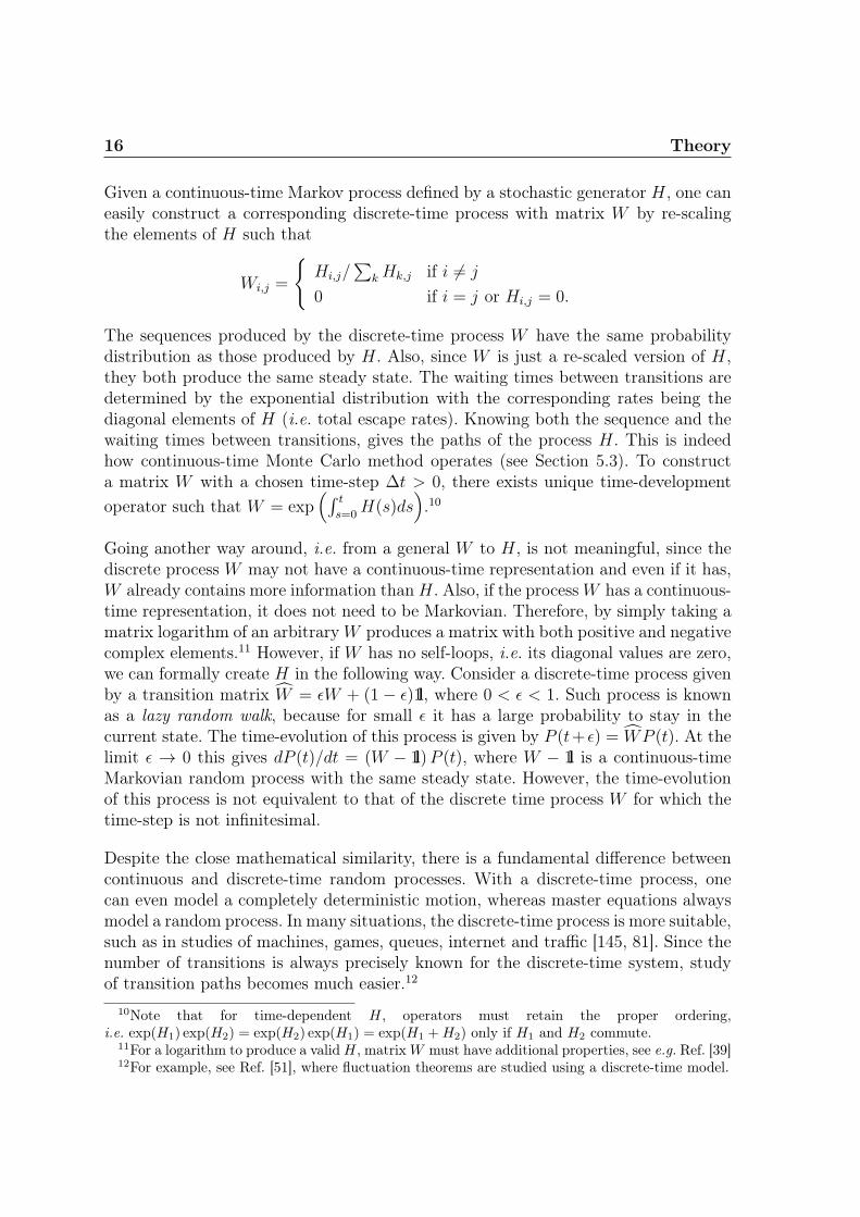
Going another way around, i.e. from a general W to H, is not meaningful, since thediscrete process W may not have a continuous-time representation and even if it has,W already contains more information thanH. Also, if the processW has a continuous-time representation, it does not need to be Markovian. Therefore, by simply taking amatrix logarithm of an arbitrary W produces a matrix with both positive and negativecomplex elements.11 However, if W has no self-loops, i.e. its diagonal values are zero,we can formally create H in the following way. Consider a discrete-time process givenby a transition matrix W = ǫW + (1 − ǫ)1l, where 0 < ǫ < 1. Such process is knownas a lazy random walk, because for small ǫ it has a large probability to stay in thecurrent state. The time-evolution of this process is given by P (t+ ǫ) = WP (t). At thelimit ǫ → 0 this gives dP (t)/dt = (W − 1l)P (t), where W − 1l is a continuous-timeMarkovian random process with the same steady state. However, the time-evolutionof this process is not equivalent to that of the discrete time process W for which thetime-step is not infinitesimal.
Despite the close mathematical similarity, there is a fundamental difference betweencontinuous and discrete-time random processes. With a discrete-time process, onecan even model a completely deterministic motion, whereas master equations alwaysmodel a random process. In many situations, the discrete-time process is more suitable,such as in studies of machines, games, queues, internet and traffic [145, 81]. Since thenumber of transitions is always precisely known for the discrete-time system, studyof transition paths becomes much easier.12
10Note that for time-dependent H, operators must retain the proper ordering,i.e. exp(H1) exp(H2) = exp(H2) exp(H1) = exp(H1 +H2) only if H1 and H2 commute.
11For a logarithm to produce a valid H, matrix W must have additional properties, see e.g. Ref. [39]12For example, see Ref. [51], where fluctuation theorems are studied using a discrete-time model.

2.2 The Master equation 17
Sequences of the discrete process
Let us consider a system described by Eq. (2.5) with time-independent rates. FromEq. (2.4) we find that the probability for a system to remain in a given state x attimes [0, t] and then jump into a next reachable state y between time [t, t+ dt] is13
P (y′, t|y, 0)dt = Hy′,y exp(−tKy)dt,
where Hy′,y is the transition rate and Ky :=∑
y′ 6=yHy′,y is the total escape rate fromthe state y.
Now consider n subsequent transitions at times t1 < t2 < · · · < tn. Such time-dependent transition series are called paths or trajectories. The path without time-stamps is called a sequence. When given an initial state x(0) at time t = 0 and timeT > 0, there are two distributions related to a sequence occurring within the time-window [0, T ]: (1) the probability f [x1, x2, . . . , xn|x0, T ] that a path is completed intime tn ≤ T such that the system stays in a final state xn for a time T − tn and (2)the probability density g [x1, x2, . . . , xn|x0, T ] that a path is completed exactly in agiven time T without waiting at the final state, i.e. the final transition to state xnoccurs exactly at T . Denoting ki := Hxi,xi−1
and Ki :=∑
j 6=iHxj ,xi−1, the latter of
these distributions can be derived [179, 161] and it is given by
g [x1, x2, . . . , xn|x0, T ] = k1k2 . . . kn
n′∑
i=1
(−1)ri−1
(ri − 1)!
∂ri−1
∂Kri−1i
[e−KiT
∏j 6=i(Kj −Ki)rj
],
where n′ is the number of distinct escape rates and ri the count for an escape rateKi, such that ri, n′ ∈ [1, n] and
∑n′
i ri = n. This weight can be also written asg(t1 + t2 + · · · + tn = T ), which is a probability consisting of n independent randomvariables. This distribution results from integrating over all transition times ti withi = 1, 2, . . . , n − 1, which can be done straightforwardly in the Laplace space. Usingthis result, probability f can be computed by integrating g [179]
f [x1, x2, . . . , xn|x0, T ] =∫ T
s=0
g [x1, x2, . . . , xn|x0, s] e−Kn+1(T−s)ds
= k1k2 . . . kn
n∑
i=1
(−1)ri−1
(ri − 1)!
∂ri−1
∂Kri−1i
[e−KiT
∏j 6=i(Kj −Ki)rj
],
where ri, n ∈ [1, n+ 1], i.e. the summation now includes also the escape rate Kn+1 ofthe final state. The exponential function contributes to the waiting time at the finalstate xn until T .
13P (y′, t|y, 0)dt = Hy′,ydt [1−Kyt/n+ o(t/n)]n
= Hy′,ydt exp(∑n−1
k=0 [−Kyt/n+ o(t/n)]), now
let n → ∞.

18 Theory
As an example, let us consider the homogeneous Poisson process for which k ≡ Ki
for all i, and xi = i is the number of discrete events. We have then n′ = 1 and r1 = nand, by using the equation above, we get
g [x1, x2, . . . , xn|x0, T ] =knT n−1e−kT
(n− 1)!,
which is a well-known Erlang distribution. For the probability f we then get
f [x1, x2, . . . , xn|x0, T ] =∫ T
s=0
knsn−1e−ks
(n− 1)!e−k(T−s)ds =
knT ne−kT
n!.
Now let us consider cycles (i.e. xn = x0) in a general Markov process. The weight ofa cycle should include three aspects: (1) The probability to be in some of the cyclestates (a starting point), (2) the probability for a complete cycle to occur, and (3) theexpected time for the completion of the cycle. Because of the Markov property, theseprobabilities are independent of each other and the result is a product of the three.The mean waiting time for a cycle is given by
∫∞
s=0sg [x1, x2, . . . , xn|x0, s] ds, which
is simply the sum of the individual waiting times∑n
i=1 1/Ki. Although this result isintuitively evident, it is not straightforward to see from a complicated formula of g,which requires ordering of the terms. This means that there is no need to computeg (or f) to find mean cycle completion time. The probability to be in one of thecycle states is simply Px1 + Px2 + · · ·+ Pxn
. Clearly the cycle probability remains thesame despite the starting point of the cycle. Finally the probability that the cycle iscompleted is given by
∏ni=1 ki/Ki, i.e. at each state the process must pick the correct
transition over others. With these three combined, we define a cycle weight
w(C) =(∑
i∈C Pi)∏
i∈CkiKi∑
i∈C1Ki
=(∑
i∈C Pi)∏
i∈C ki∑i∈C
∏j∈C,j 6=iKj
. (2.8)
The dimension of this weight is inverse of time, so it could be called a cycle rate. Thisweight defines a type of a measure that one can use to compare cycles. For example,by multiplying w(C) with a total center-of-mass displacement during the cycle, onereceives a new weight corresponding to average transport velocity over the cycle. Fornonequilibrium systems, w(C) depends on the direction of the cycle and the ratiow(C)/w(C) =
∏i∈C ki/ki, where ki indicates the corresponding inverse rates for the
inverse cycle C, differs from the unity. Using this cycle weight, one may compare cyclesand, more importantly, find the ones that correspond to the largest (or smallest) cycleweight.

3 Models
In this Chapter, we describe the observables and models on which we shall concen-trate in this Thesis. We start by defining the underlying lattice and the types of thepotential. After this, the observables of interest are defined. Finally, the models forlinear polymers and single-layer atomic islands are defined.
3.1 External potentials
In order to study long-time center-of-mass transport, models studied in this work areplaced on infinite one or two dimensional lattices. Without loss of generality, we fix thelattice constant (i.e. the spacing between nearest-neighbor sites) to 1. For a periodicpotential, it is equivalent to study a model confined in a single period of the potentialand apply periodic boundary conditions. For a one dimensional periodic potential,this means V (x+ L) = V (x), where L > 0 is the spatial period. In higher dimensionsthere, might be several period lengths depending on the potential and the geometry ofthe lattice. The stochastic generator H only needs to include potential states within asingle period. If the potential is homogeneous in space (e.g. only external fields exists),one can take L = 1.
The assumption of infinite lattice is a good approximation for real systems if themedium is much larger than the period length and the size of the moving objectof interest. This is indeed the case with most microscopic systems, where the movingobjects are in molecular or atomic scale. Then one can limit the study to steady statesof the periodic systems and neglect boundary effects.1 This approximation is essentialto keep the size of the state space of the system reasonable. Therefore in majority oftheoretical studies of transport in microscopic systems, such as Brownian/molecularmotors and the ratchet effect, periodic boundary conditions are assumed [148].
In this work, we consider two types of external potentials: (1) non-homogeneous po-tentials that are periodic in space and time, for which we apply notation V (x, t), and(2) spatially homogeneous time-dependent fields, which we denote by E(t). For V ,we consider flashing and traveling potentials (see Section 2.1.4), and for E, we con-sider both static and time-dependent potentials. Potentials are temporally varied by
1However, boundary effects are important when studying transport in two and three dimensionswith confined space, such as tubes [2].
19

20 Models
switching cyclically between two different potentials. This switching process is eitherinstantaneous or smooth in time. We shall consider both stochastic and deterministicswitching in the instantaneous case.
3.1.1 Deterministically time-dependent potentials
When the temporal variation of the potential is periodically deterministic, the gen-erator has the property H(t) = H(t + τ), where τ > 0 is the temporal period. Forthe special case of instant switching, rates Hy′,y(t) are piecewise constant functions intime and the stochastic generator is given by
Hy,y′(t) =
H1y,y′ , t ∈ [0, τ1)
H2y,y′ , t ∈ [τ1, τ1 + τ2)...
HSy,y′ , t ∈
[∑S−1s=1 τs, τ
),
(3.1)
where, for s = 1, . . . , S, the matrix Hs is the time-independent stochastic generator inthe potential Vs (all having the same spatial period) and the lifetime of the potentialis τs, with the total period being τ =
∑Ss=1 τs. This type of potential switching,
where the order of the potentials is fixed, is called cyclic (i.e. V1 → V2 → . . . VS →V1). In this work, we call these instantaneous types of time-dependent potentials asdeterministic potentials (in Article II these are known as Type 2 potentials). A specialcase of this is the on-off potential with S = 2, V2 ≡ 0 and V1 6= 0, which is the workingprinciple of the flashing ratchet defined in Section 2.1.4.
In addition to non-continuous switching, we also consider the following smoothly vary-ing potential V (x, t) = V1(x, t) sin
2(πt/τ) + (1 − sin2(πt/τ))V2(x, t). In this scheme,potentials V1 and V2 alternate smoothly and symmetrically, such that the time av-eraged potential is simply (V1 + V2)/2. We call this a smoothly varying potential (inArticle II this is known as Type 3 potential).
3.1.2 Stochastically time-dependent potentials
Instead of periods τi being fixed for the instant switching scheme (3.1), they couldalso be random variables. If the distribution of random periods τi is not an exponen-tial distribution, i.e. switching is non-Markovian, the time-evolution is governed by ageneralized master equation [96], which includes memory-effects and is hard to solveeven numerically. For Markovian switching, i.e. when the waiting time distributionis exponential, potentials can be directly included into the master equations without

3.1 External potentials 21
time
stochastic deterministic smoothlyvarying
Figure 3.1: An illustration of the time-evolution of maxx [V (x, t)] for three types of potentials inthe case S = 2.
need for generalized master equations. Then the problem turns into solving an aug-mented set of master equations for the probabilities Py,s(t), where s is the state ofthe potential. The augmented stochastic generator H remains independent of timeand the system is directly solvable via solving the eigenstate corresponding to thesteady state (see Section 2.2.3). In addition to being computationally easy to handle,Markovian switching is a good approximation for many naturally occurring potentials.For example, the ATP-ADP energy cycle in cells is essentially Markovian. Because ofthese properties, Markovian time-dependent potentials are applied in majority of theratchet effect studies [148]. In this work, we shall call potentials with Markov typetemporal periods and instantaneous switching, as stochastic potentials (in Article IIthese are known as Type 1 potentials).
For the Markov type cyclic switching, the augmented stochastic generator correspond-ing to the deterministic one in Eq. (3.1) is
dPs,y(t)
dt=∑
y′ 6=y
[Hs
y,y′Ps,y′(t)−Hsy′,yPs,y(t)
]+
1
τs−1
Ps−1,y(t)−1
τsPs,y(t),
where τs is the expected lifetime for a potential s, and the periodicity τ0 = τS isapplied. Since the time periods are random, one may expect that the average responseof the system as a function of τ becomes smoother, because of mixing of time-scales.When compared to deterministic potential, there is more variation in paths, whichrequires more iterations when determining expectation values with the Monte Carlomethod. See Fig. 3.1 for an illustration of all three time-dependency schemes for thecase S = 2.
3.1.3 Simple limits of the temporal period
When studying time-dependent potentials, it is useful to first consider simple limitsof the temporal period τ . Let us first consider the case τ → 0, such that τi > 0 for all

22 Models
1 ≤ i ≤ S. In this case, the very rapidly changing potential becomes an effective mean-field potential, and the dynamics is generated by the mean-field stochastic generatorH. For deterministic potentials that vary smoothly in time, the mean-field operatorhas elements
Hy′,y =1
τ
∫ τ
0
Hy′,y(t)dt.
For instantaneous type deterministic and stochastic potentials, elements reduces intoHy′,y =
∑s τiH
sy′,y/τ , where τi/τ ’s are the weight factors. Long-time expected values
can be computed using the steady state of the generator H. Although this limit ismathematically well defined, from the physical point of view it is artificial, because forreal systems, there is a finite response time for changing the potential state (e.g. chargere-distribution to build up an electric field) and for an object to respond (e.g. inertia).If these effect are taken into account, it means that no net transport is expected tooccur at the limit of very fast switching.
Now assume that τ is very large.2 For instantaneous type deterministic and stochasticpotentials, the system converges (arbitrary close) towards the steady state, before thepotential is switched again (e.g. ’on’ or ’off’ for a flashing ratchet), and the time spendin the transient state becomes negligible. For smoothly varying potentials, the systemremains very close to equilibrium at all times. The expected values of observablesapproach their adiabatic values, that, for smoothly varying potentials, are computedwith
〈O〉 = 1
τ
∫ τ
0
〈O(t)〉ssdt,
where 〈O(t)〉ss is computed using the steady state of the operator H(t). For instanta-neous type deterministic and stochastic potentials, the computation again reduces into〈O〉 =
∑s τs〈O〉s/τ , where 〈O〉s is the expected value of the measurement operator
computed in the steady state of the generator Hs.
When it comes to transport, the special interest lies in the situation with non-zero nettransport for finite values of τ , while it disappears at τ → ∞. For instantaneous typedeterministic and stochastic potentials, the transport for large τ is then governed bythe relaxation behavior occurring at the switching of the potential. Let dj,i denotethe expected travel distance of the center-of-mass within the potential j, using thesteady state of the potential i as an initial state and then letting the system fullyrelax. For cyclic switching, summing over all dj,i’s then gives the total expected traveldistance within one complete period τ . Travel distance during one cycle is given by d =∑S
i=1 di,i+1. Because of the finite relaxation times for all real systems, d can be alreadycomputed by considering time-scales of the order of the largest relaxation times inthe system. Therefore, for very slow switching, the velocity can be approximatedby the adiabatic velocity vad = d/τ . For complex systems, even the sign of vad is
2For instantaneous type deterministic and stochastic potentials, also all τs’s for s = 1, . . . , S areassumed large separately. If ratios τs/τ ’s are kept fixed, this will inevitably happen when τ gets large.

3.2 Observables 23
generally unknown beforehand. This is often the situation when studying the ratcheteffect and will be studied further in Chapter 6. For a smoothly varying potential, thesituation is somewhat more complicated, since the potential is constantly changing.If one assumes that the system remains all the time arbitrary close to equilibrium,the velocity is always zero and so one also gets d = 0. However, for certain types ofpotentials, there exists so called reversible transport and one can obtain a non-zero deven while doing the computation at equilibrium [131].
3.2 Observables
In addition to probabilities Py(t) themselves, the most interesting information lies indifferent types of observables. In this work, we are mainly interested in transport prop-erties, namely the velocity and diffusion properties. For objects that are deformable(i.e. not point-like), such as polymers and atomic islands, other interesting observablesare the size and shape of the object.
From theoretical point of view, the two types of observables are different: transport-related observables depend on the paths taken by the stochastic system (e.g. thevelocity and diffusion) and other observables depend only on the probabilities Py(t)(e.g. shape and size measurements). In addition to transport properties, for exampleenergy consumption and entropy production of the system belong to the first category.Path dependent observables are more complicated to compute, since they cannot bemeasured directly from probabilities. Probability-dependent observables are easier tocompute, but the construction of their measurement operators can still be compli-cated, especially when using the recursion method (see Section 4.1.1).
3.2.1 Velocity and diffusion coefficient
The transport properties of the object are computed from the time-dependent center-of-mass distance vector x(t). For the steady state, the velocity v and the effectivediffusion coefficient Deff are defined as
v = limt→∞
〈x(t)〉t
Deff =1
2dlimt→∞
1
t
[〈x2(t)〉 − 〈x(t)〉2
],

24 Models
where d is the dimension of the system. These definitions are usually applied whenusing the Monte Carlo method. Derivative forms of the previous are
v = limt→∞
1
τ
∫ t+τ
t
d〈x(s)〉ds
ds
Deff =1
2dlimt→∞
1
τ
∫ t+τ
t
[d〈x2(s)〉ds
− 2〈x(s)〉d〈x(s)〉ds
]ds,
which are useful for systems with temporally periodic deterministic potentials, espe-cially when using the master equation method. Equivalence of these two definitionscan be easily shown by differentiating the first formulae or using integration by partsto the latter one. In practice, it is enough to take a large enough t such that the steadystate is reached within required numerical accuracy. We also define the Peclet number
Pe =|v ℓ|Deff
,
where ℓ is the length scale of interest of the transport, such as the size of the objector the spatial period of the potential. The Peclet number is a dimensionless measureof the transport coherence. For perfectly deterministic transport, one has Deff = 0and thus the Peclet number diverges, which means that the transport is completelycoherent without any fluctuations.
3.2.2 Energetic efficiency
Keeping up a nonequilibrium state requires energy. Especially for non-artificial molec-ular motors working in the cells, the efficiency is essential because of the limited energyavailable [11]. It is also an interesting aspect for artificial motors. However, the defi-nition of the efficiency is complicated for microscale systems. In the literature, severalkinds of definitions of the efficiency have been proposed for Brownian motors, whichare not directly comparable against each other [148, 185, 132, 45, 189, 180]. We arenot aware of any work in which several measures of efficiency would have been sys-tematically compared on the same model. Here we adopt the basic thermodynamicdefinition based on the work done against an opposing force F , i.e. the output powerof the motor is given by vF , where v is the average velocity. The input power Win
comes from externally induced potential state changes, which force the traveling ob-jects in a higher energy state depending on its position with respect to the potential.This approach is different from the other proposed scheme, where the object gainsconstant amounts of energy by, e.g. ATP hydrolysis, regardless of the location. Weassume that the energy becomes dissipated into the environment, when the objectreturns to a lower energy state, i.e. this energy is not reduced from the input energy.

3.2 Observables 25
For cyclically changing potentials, we define the steady state input power as
Win =
∑Ss=1
∑y max
[0, Es+1
y − Esy
]τ−1s Ps,y stochastic
1τ
∑Ss=1
∑y max
[0, Es+1
y − Esy
]Py(∑s
k=1 τk) deterministic1τ
∑y
∫ τ
t=0max
[0, dEy(t)
dt
]Py(t)dt smoothly varying,
where Esy is the total energy of the microstate y in the potential s, and similarly Ey(t)
is the total energy at time t. The efficiency is defined by η = vF/Win. This definitionis applied to compute energetic efficiency of the flashing ratchet transport (see Section6.5).
It has been found, that some real-life molecular motors can exhibit very large efficien-cies, e.g. around 60% for Kinesin and up to 90% for F1-ATP [56]. When comparedto these, the efficiency of the flashing ratchet model is very low for single particles(see e.g. Ref. [132]), but it can be greatly increased for some many particle systems[169, 190]. Despite the size of the machine, the trade-off must be made between theenergetic efficiency and the speed; increasing the first, typically decreases the latter.Indeed, the reversible ratchets that operate near equilibrium exchibit efficiencies near100% while being extemely slow [131].3
Besides the efficiency, we are also interested in the stopping force Fstop which, whenapplied, causes the long time velocity go to zero. The larger Fstop is, the stronger themolecular motor is. For example, it has been found in Ref. [54] that for polymersworking as Brownian motors in the flashing ratchet, Fstop depends on the length ofthe polymer by increasing as the polymer gets longer.
3.2.3 Shape deformations
For systems containing deformable objects, the observables related to the size andshape may carry interesting information. This is especially true if their shape deforma-tions are directly connected to the transport properties, i.e. objects move by changingtheir size and shape instead of sliding. To compute these observables, some effort mustbe made to create operators for them, or measure them from the simulations. Whenusing the master equation method, expectation values and their fluctuations can becomputed as explained in Section 2.2.3 as these types of observables do not dependon paths. Both steady state and transient expected values are of interest. In Chapters6 and 7, we study the shape deformations of polymers and atomic islands.
3For a reversible ratchet, both v and Win approach zero at the adiabatic limit such that theirfraction remains non-zero.

26 Models
3.2.4 Relaxation time
When a physical system is pushed out from its steady state, it takes some time beforethe system can return into the steady state. Responses to the perturbations are neverimmediate. Given two events or measurements of the system temporally close to eachother, there is always some amount of correlation between them. The average timerequired to return back to steady state after perturbation, or to correlations to wearoff, is called the relaxation time. A system can contain several relaxation times, relatedto different processes and observables. The longest of these times is called the leadingrelaxation time. Roughly speaking, the leading relaxation time defines the maximumtimescale needed for the process to ’forget’ its initial state and to become uncorrelated.
For stochastic processes the relaxation time is defined for distributions in the sensehow fast they decay, i.e. |P (t)− Pss| → 0, where Pss is the steady state. Especially inmathematics, this is also called mixing. For master equations, the relaxation times aregiven directly by the eigenvalues λi of the stochastic generator H (see e.g. [113, 117]).This can be seen from the transient solution (2.6). The real parts of λi are alwaysnegative and the relaxation times are defined by 1/|Re(λi)|. The leading relaxationtime is therefore given by the inverse of the largest non-zero eigenvalue, i.e. the spectralgap between the first and the second eigenvalue. If H includes both the potential withsome spatial length (i.e. L > 1) and an object with internal states, the relaxationtimes describe both internal and spatial relaxation.4
The leading relaxation time is the property of the master equation set and is indepen-dent of the initial state, hence it is not directly related to the relaxation time found inexperiments or simulations where one usually measures the relaxation of some macro-scopic observables, such as the shape and size of deformable objects [36]. Instead, it isrelated to the computational effort of finding a steady state using numerical methods,such as integration and iterative eigenstate solvers (see Chapter 5). As the leadingrelaxation time increases (i.e. the second eigenvalue approaches zero), the search forthe steady state becomes more time-consuming and error-prone.
3.3 The Rubinstein-Duke model
Reptation theory describes the rheological behavior of linear polymers in conditionswhere the density of obstacles such as other polymers or pores of the medium is veryhigh. In such conditions only the polymer heads are able to move into previouslyunoccupied space, thus creating a ’tube’ for the polymer to move back and forth.
4This situation arises, for example, for the repton model studied in Chapter 6 with periods L = 3and L = 6.

3.3 The Rubinstein-Duke model 27
The polymer motion under these conditions is called reptation. In the first theoreticalstudy of the reptation in 1970s, de Gennes predicted scaling laws for the dependenceon the polymer length L for viscosity (i.e. the tube renewal time) scaling as ∼L3 andthe diffusion constant scaling as ∼L−2 [67]. These assumptions were later confirmedwith experimental and computational methods [104, 116]. One of the most notablecomputational models for reptation was proposed by Rubinstein in 1987 [156]. In hismodel, the network of obstacles is modeled by a lattice and, by assuming that thecorrelation length between the polymer segments is smaller than the distance betweenthe lattice sites, the problem can be discretized to a simple particle hopping model.In 1989 Duke extended this model by allowing it to include an external field [55], thusgiving birth to the Rubinstein-Duke (RD) model. Soon after this, theoretical researchof the model started to flourish. The main interest has been in the scaling of thediffusion coefficient and the relaxation time as a function of polymer size, and alsothe behavior under static fields (see Ref. [110] for a review of results and models). Theoriginal RD model can be easily extended by adding external potentials and modifyingthe rules. Our aim is to study the RD and its modification in non-homogeneous time-dependent potentials. Technical details and the stochastic generator of the RD modelare described next.
3.3.1 The stochastic generator
In the RD model, the polymer is divided into N units, called reptons, which occupythe sites of a regular 1-3 dimensional lattice. The number of reptons that each site canaccommodate is unlimited and self-avoidance effects are neglected. Each configurationis projected onto an axis along the diagonal of the unit cell and it is identified by therelative coordinates yi = xi+1 − xi of neighboring reptons along the chain, where xiindicates the projected coordinate of the ith repton. The relative coordinates can takethree values yi ∈ −1, 0, 1 and there are thus in total 3N−1 different configurationsfor a chain with N reptons. See Fig. 3.2 for an illustation of this mapping procedure.When two or more reptons accumulate at the same lattice site, they form part of astored length, which can then diffuse along the tube. In terms of relative coordinatesa segment of stored length corresponds to yi = 0 and therefore allowed moves areinterchanges of 0’s and 1’s, i.e. for adjacent reptons (yi, yi+1) = (0,±1) ↔ (±1, 0). Onthe other hand, the end reptons of the chain can stretch 0 → ±1 or retract ±1 → 0to the site occupied by the neighboring repton. The dimension of the medium (beforethe projection), enters the RD model by modifying the transition rates of the headreptons. This is the standard RD model.
In order to study the effect of the intrinsic transition rules of the reptons in time-dependent potentials, we will compare the results for the RD model with the results ofa non-reptating polymer allowing the breaking of the tube. With the above definition,

28 Models
x
0 1 0 0 1 -1 -1 -1 0 1
Figure 3.2: An illustration of the Rubinstein-Duke model (right) as a projection of the reptation intwo-dimensions (left). In the Rubinstein-Duke model, black arrows indicate reptation moves, whereasthe moves with blue arrows are for the relaxed model (see text).
moves with (0, 0) ↔ (±1,∓1) are also allowed. We call this relaxed model the free-motion model (FM model). Dynamics of the FM model is similar to that of theclassical Rouse polymer model, where the polymers are not restricted into tube andcan also move freely sideways [154]. In Fig. 3.2, black arrows indicate allowed moves forboth models, whereas the moves with blue arrows are only allowed in the FM model.The stochastic generators for the RD and FM models only differ such that there aremore non-zero matrix elements for the FM model. Similar types of extensions andmodifications of the RD model have been previously studied in different contexts[130, 53, 164]. In this work, we use a generic term repton model to include both RDand FM model.
Technically, the repton model is similar to a quantum mechanical open spin-1 chain,which consists of N − 1 sites with three possible states (+1, 0 or −1) and interactionsdescribed above. Because of the nearest-neighbor interaction, the repton model hasa compact and simple operator representation which enables a recursion method inbuilding of the operators (see Section 4.1.1). Any operator in the repton model canbe constructed using local 3× 3 sized operators that operate on the individual bondsbetween reptons (i.e. values of yi). In the space of the complete polymer, these localoperators (X) have a tensor product form given by
Xi :=
[i−1∏
k=1
1l3⊗]X
[N−1∏
k=i+1
⊗1l3
],
where N is the number of reptons. The dimension of Xi and the stochastic generator

3.3 The Rubinstein-Duke model 29
itself is 3N−1. To consider the polymer dynamics in a non-homogeneous medium withthe potential V (x) = V (x+L), in addition to the internal state of the potential, alsothe external state of the potential must be added to all operators. For this purpose,one marker repton, which gives the spatial location of the polymer with respect topotential, must be chosen. Although we are free to choose any repton [103], choosingone of the head reptons is most convenient. Choosing the left head repton, all operatorsthen have the form Yl⊗Xi, where the L×L-sized local operator Yl works in the state-space of the potential and gives the spatial location. The state of the polymer has therepresentation
|marker repton〉 ⊗ |polymer configuration〉 = |Φl〉 ⊗ |Ψy〉,
where |Φl 〉 has dimension L and |Ψy〉 has dimension 3N−1. The stochastic generatorof the repton model in periodic potential can be cast in the form
H(t) =L∑
l=1
[Al(t) +
∑
y
(By,l(t) +
N−2∑
i=1
Mi,y,l(t)
)], (3.2)
where the operators A and B are responsible for the dynamics of the heads and theoperator M creates the dynamics for the bulk reptons. The reptons are assumed tocarry charges which are affected by external potentials. When no external potentialsexist, rates for all available transitions are set to 1. Existing external potentials mod-ify the rates according to the Kramers rate theory (see Section 2.2.2). We considermodels with both uniform and non-uniform repton charge distributions. The detaileddefinition of operators and their practical construction are given in Section 4.1.1.
3.3.2 Observables of interest
Properties of the RD model at equilibrium and in static field are well known. At equi-librium (i.e. no external potentials), the leading behavior for the diffusion coefficientis DN ≈ [(2d+ 1)N2]
−1, where d is the dimension of the medium, and for the tubereneval time (the relaxation time) τ ∝ N3. The behavior of τ has been found to be sen-sitive to dimension d, since lowering d leads to larger exponent for the relaxation [25].By allowing additional movements to standard RD model, the cross-over from the rep-tation towards Rouse dynamics with DN ∝ N−1 and τ ∝ N2 occur [53]. In large staticfields, RD polymers create V-shaped trap configurations5, which causes the velocityto decay exponentially towards zero as the driving field is increased [193, 102]. As theforce affecting the polymer depends on the total charge of the polymer, the velocityfor large polymers can become decreasing already in small fields. This slowing-down is
5Trap configuration are states which require lots of energy to escape from. Without escaping atrap configuration, the transport cannot occur.
30 Models
a problem for the applicability of experimental techniques such as gel-electrophoresis,which is used to sort the DNA chains according to their length [172]. The phenomenonwhere polymers with different lengths move equally fast (or slow) in a field, is knownas the ’band collapse’ and when this occurs, polymers cannot be separated based ontheir length.
The situation is, however, completely different when the static field is replaced witha time-dependent non-homogeneous potential. The velocity and diffusion propertiesof such system are very hard to predict because of the complex temporal and spa-tial interaction between the polymer and the potential. The transport properties aretherefore our main interest. Some of the previous work involving polymers and time-dependent fields have shown some interesting properties, such as current inversions[134, 54, 97]. Also experimental research has been conducted by considering separatingof DNA by utilizing the ratchet effect [13].
Among other interesting observables are the Peclet number and energetic efficiencyof the polymer transport. In order to study the correlation between the shape defor-mation of the polymer and center-of-mass velocity, we also define the following oper-ators: the zero-bond count (number of 0-bonds), the kink count (number of (+1,−1)or (−1,+1) bond pairs), the head-to-head length (distance |x1−xN | between first andlast repton) and the total length (maximum distance maxi,j (xi − xj) between any tworeptons). The corresponding operator definitions and their recursive construction ofthese observables are found in Section 4.1.1. For example, for the configuration inFig. 3.2 the values for of these operators would be 3 for zero-bonds, 1 for kinks, 0 forthe head-to-head length and 3 for the total length. Separating the head-to-head andthe total length is important since it provide a means of distinguishing between linearand bent (such as V and U shaped) conformation of the polymer.
3.3.3 Non-uniform charge distributions
The usual assumption in the studies concerning polymer transport is that the polymeris homogeneous, i.e. in discrete models all monomers are identical with the same chargeand mass. We shall relax this assumption and study the effect of the non-uniformcharges for the repton model. Previous works on the RD model have considered someaspects of this. In Ref. [25], a magnetophoresis model (i.e. one charged head repton)was considered, and in Ref. [52], it was shown that when it comes to the velocity,all charge distributions are equivalent in small fields (i.e. linear response regime).6 InRef. [150], it was noticed that the drift in constant field depends strongly on the posi-
6This is clear, since in the linear response regime only the total force affecting the object matter,and the diffusion coefficient is given by the Einstein relation. Similar equivalence does not hold forsystems involving non-homogeneous potentials.

3.4 The model for single-layer metal islands 31
tion of the charged repton within the polymer, and in Ref. [102], non-homogeneouslycharged RD polymers in large fields were studied. A recent study of dimer kinetics ina periodic potential shows that if the connected particles are non-identical, directeddrift can be generated even in a symmetric potential [68].
We want to find the optimal charge distributions for the RD and FM polymers whichresults in the largest possible drifts. The optimal charge distribution can be expectedto give some (indirect) information about the polymer conformations and reptons thatdominate the transport (i.e. have the largest impact on the velocity). Optimizationof periodic potentials has been previously considered for single particle systems [18,49, 199].
3.4 The model for single-layer metal islands
Diffusion of adsorbates is perhaps the most elementary transport process occurring onsurfaces [86]. It is crucial for more complex surface phenomena, such as crystal growth,associative desorption, heterogeneous catalysis and chemical reactions. We are inter-ested in the diffusion of metallic atom islands on a smooth surface. In the basic setup,the island consists of single layer of atoms lying on the surface of the bulk materialconsisting of similar atoms. Atoms move in hopping manner between the minima ofthe regular surface potential created by the bulk atoms and the island. Equilibriumproperties of these type of systems are well known, as well as near-equilibrium proper-ties under small electromigration forces7 in the linear response regime [5]. Also someproperties under strong forces have been studied with continuum models [137]. We areinterested in the properties of single-layer atom islands under the effect of strong andtime-dependent external forces, in particular, in the behavior of small islands withup to 20 atoms, where the discreteness and finite-size effects are strongly present andetropic effects are not yet dominant. We apply an idealized model of hopping atomsin the square lattice with nearest-neighbor energetics [123]. Technical details and thestochastic generator of this model are described next.
3.4.1 The stochastic generator
The model consists of two-dimensional atom islands on an unbounded square-latticesurface. In this set-up, each atom has up to four nearest and four next-nearest (di-agonal) neighbors. To keep the islands unbroken, we require that each atom must beconnected to the island with at least one diagonal neighbor. The dynamics is created
7Electromigration force is the force caused by collisions between the atoms of the island andfield-driven electrons in the bulk.

32 Models
(3)(0)
(1)
(2) αγ
Figure 3.3: An illustration of the model with a 6-atom (N = 6) island going through 4 consecutivetransitions and used notation for the angles γ and α (see text). Small arrows indicate the transitionsand their corresponding values of the ∆f,i parameter in Eq. (3.3).
by single atom hops in continuous time with rates given by a semi-empirical modelparameterized by the embedded atom method [123]. Within this model, the changesin the binding energy for an atomic transition is computed from the change in thenearest neighbor atom count. Despite its simplicity, the energetics given by the modelis in good agreement with molecular dynamical computations (see [98] for the mostrecent results). The transition rate Γi,f from the initial state (i) to the final state (f)is given by
Γf,i(t) = ν exp
(−ES −max 0, EB∆f,i+ Ef,i(t))
kBT
), (3.3)
where ν is an effective vibrational frequency, ES is the energy barrier for the atomtransition along the island edge, EB∆f,i (∆f,i = −3, . . . , 3) is the change in the bindingenergy with nearest neighbor bonds, and Ef,i(t) gives the time-dependent contribution(positive or negative) to the transition rate by an external electromigration-type forceand depends on the magnitudes and directions of the field and atom displacement.The model and its parameters are illustrated in Fig. 3.3.
For Cu on Cu(001) we use EB = 0.260 eV and ES = 0.258 eV [123]. We set νand the lattice constant to 1. Since the barrier ES appears in all transitions, it canbe integrated in the prefactor by defining a new temperature-dependent prefactorν := ν exp(−ES/kBT ). Due to the large separation of energy barriers, there are attemperatures T < 1000 K four well-separated microscopic rate parameters in thesystem in zero field and up to six for large fields (E ∼ EB) in the direction of the mainaxes of the lattice. Depending on the direction of the field, the energetics gets morecomplicated as demonstrated in Fig. 3.4, where we have plotted all 16 unique ratesΓf,i that appear for the case E > 0 and α = 23. Although experimentally realizableelectromigration forces in most cases are too small (order 10−5 eV [122, 153]) to causesignificant non-linear effects alone, combined with other methods that can decreaseenergy barriers, such as strain, manipulation with scanning tunneling microscopy andelectric fields [136, 78], non-linear effects are expected to emerge.
Although this simplified model is not microscopically accurate, it captures the key

3.4 The model for single-layer metal islands 33
0 0.05 0.1 0.15 0.2 0.25
10−10
10−5
100
E
Γ
Figure 3.4: Separation of time-scales in terms of possible jump rates Γ for the island model as afunction of the field strength at temperature T = 500 K for field direction α = 23 (see Fig. 3.3 forthe definition of the angle α).
elements of the dynamics, respects the detailed balance condition (for Ef,i(t) ≡ 0)to avoid spurious currents and is straightforward to apply in computations. We wantto apply a simplified model as we do not wish to study only a particular systembut rather to investigate properties which should not depend on the finest detailsof the atom-atom interaction. Therefore, we use a simple kinetic model containingas few parameters as possible. Since experimentally realizable field amplitudes inelectromigration are really small, transport properties of non-continuous islands havebeen previously studied only within the linear-response regime with very small fields(E < 0.01 eV).
As the detachment of atoms from the island is forbidden in our model, the numberof atoms in the island remains a constant. This is a well-justified approximation forsmall fields (i.e. Ef,i ≪ EB) and temperatures far below the melting point of the metal(1358 K for Cu). Also, if the density of free surface atoms is such that evaporationand condensation are balanced, the island size could be kept constant on averagealso with unrestricted dynamics. When the detachment/attachment processes are rarecompared to other processes, the properties of the variable size islands follow fromthose of the fixed size islands, because the island size remains fixed for long periodsof time, thus allowing relaxation between events. In such cases, for example the meanvelocity of the variable size island under a driving force is a combination of velocitiesof fixed size islands over a wide time scale. Only when the detachment/attachmentprocesses become very frequent, which necessarily occurs at high temperatures andvery strong fields, this commonly used picture of noninteracting islands with differentsizes is no longer valid. On the basis of previous studies at (or near) equilibrium

34 Models
(e.g. [167, 80]) and the results of Chapter 7, at least within temperatures below800 K and E < 0.1 eV one can assume that the dynamics is not dominated bythe detachment/attachment processes and island transport is mainly controlled bythe periphery diffusion.
The velocity of the center-of-mass of the island is given by a vector ~v = (vx, vy) and ~x =(x, y) is the center-of-mass position at the surface using the main axes of the lattice.We define the measuring direction by angle γ, i.e. we measure v = vx cos(γ)+vy sin(γ).The field is defined by the amplitude E ≥ 0 and the angle α of the field direction,i.e. ~E = (E cos(α), E sin(α)). The effective diffusion coefficient Deff can be computedwith a projected distance xγ = cos(γ)x+ sin(γ)y.
To illustrate atomic transitions and the effect of the field, consider a non-zero fieldwith α = 90 such that ~E = (0, E)) in Fig. 3.3. The energy barriers for the fourtransitions shown are decreased by E and similarly increased for the correspondinginverse transitions. For α = 45, the barrier of transition (1) is decreased by 2E/
√2
and that of transition (0) by E/√2. In what we shall call the Monte Carlo (MC)
model, two independent separate jumps are required to go around a corner [processes(1)-(3)], whereas in the Master Equation (ME) model such transitions occur by directdiagonal jumps.
3.4.2 The reduced model
The number of configurations for two dimensional islands becomes huge even for smallnumber of atoms. To be able to study islands up to N = 12, we reduce the number ofisland configurations by allowing only states that do not include configurations withonly diagonally connected atoms or parts of the island. To facilitate going aroundthe corner, which is necessary for long-range transport of the island, we allow directdiagonal jumps like those shown in Fig. 3.3 (numbers (1-3)). In the MC model, goingaround the corner is possible by two jumps. The energy barrier of the diagonal jumpis approximated by a sum of the binding energy difference between the initial and theintermediate state and the energy difference caused by the field. Further reductionwas made by disallowing vacancies (i.e. holes) inside the islands, which however onlyhas a minor effect on the number of available states. This way we have defined theME model.
These approximations cause only minor differences between MC and ME models inequilibrium (E ≡ 0), where the weights only depend on the total energy of the con-figuration, and the islands prefer compact rectangular shapes. For nonequilibriumstates, major differences between the models are expected, especially for field ampli-tudes approaching the binding energy E ∼ EB. This is mainly because of the trapconfigurations and the diagonal jump approximation. The difference between the MC

3.4 The model for single-layer metal islands 35
and ME models depends on how important the corner states are for the dynamics.
The allowed island configurations are known as polyominoes (or lattice animals), andtheir counting and statistical properties are known at least up to N < 47 [90]. Sincethe practical limit for numerical master equation computations is about 106 states, thelargest system studied in this work is the 12-atom island with 468837 states (505861if vacancies are allowed). From now on, we call this reduced model the ME model ,whereas the full model is called the MC model . For a comparison, only up to 8-atomislands could be treated by applying the ME method directly to the full MC modelwithout any above reductions (see Section 4.1.2 for details). The ME model does nohave the kind of compact operator representation as the repton model has, thereforewe rely on an enumeration method in creating the stochastic generator H and otheroperators. This is covered in Section 4.1.2.
Neither the numerical master equation nor Monte Carlo method can be applied assuch to study properties of the islands at very low temperatures. As the temperaturedecreases, the difference between the largest and the smallest rate increases, whicheventually leads to a very stiff set of linear equations (i.e. H is badly scaled). Thislimits the minimum temperature for practical computations to be around 500 K. Whencomputing the steady state (i.e. solve Hx = 0), the stability of computations can besomewhat improved by using a diagonal pre-conditioning matrix with entries 1/Hi,i
(this works because H is weakly diagonally dominant). This decreases the lowestreachable temperature to be near 300 K for the velocity. However, this procedurewas not generally found to improve computations of the effective diffusion coefficientthat requires solving linear equations of the type Hx = b (additional details in Section4.2.1). In general, reaching low temperatures with stable numerics would require coarsegraining techniques to reduce the separation of rates, and it is a possible continuationfor this work.8
3.4.3 Observables of interest
Equilibrium properties of islands (and also voids) are well known [5, 198, 183, 80].For example, the center-of-mass diffusion coefficient for large islands is proportional toe−Eeff/kBTN−α, where Eeff is an effective Arrhenius barrier and α is a scaling exponent.In most situations the most important diffusion mechanism is the periphery diffusionfor which α = 3/2 and Eeff ≈ 0.75 eV have been obtained. For small islands upto 20 atoms or so, many-body effects have a dominating role and there exist strong’magic size’ effects, hence the diffusion coefficient is strongly size dependent. For smalldriving forces, large islands become deformed and move with an oscillatory fashion
8This kind of idea has been applied in Ref. [163], where low temperature coarse graining is carriedon by hand for islands N = 3 . . . 5.

36 Models
[122, 20, 157, 153].
Our main interest lies in the steady state velocity as a function of field direction α,amplitude E and temporal period τ . For time-dependent fields, island transport be-comes also frequency dependent. Due to the interplay between island configurationsand strong time-dependent forces, one could expect phenomena such as current in-version or increase to appear (see e.g. Ref. [134, 3]). Because of the square latticegeometry, the (001) surface is a good candidate for investigating the effects of rotatedfield, which would be less pronounced for e.g. the (111) surfaces. The relationshipbetween transport properties and these parameters has not been systematically stud-ied beyond linear response regime. We are also interested in shape deformations ofthe islands, such as the average thickness and length in the direction of an axis, therelaxation time and the effective Arrhenius barrier in strong fields.

4 Setting up the equations
In this and the following Chapter, we describe the numerical methods used in thiswork. The main emphasis is on the direct numerical solution of master equations, butalso the Monte Carlo method is discussed. In this Chapter, we cover the construction ofmaster equation sets and derivation of equations related to the observables. Solvingthese equations is discussed in the following Chapter. Explicit construction of themaster equation set is necessary to find a numerical (or algebraic) solution usingthe linear algebra, whereas in the Monte Carlo method, master equations are formedimplicitly during the computation.
4.1 Constructing the master equation sets
The first step of the numerical master equation method is to build and store theequations. Master equations and operators are written by using the sparse matrixrepresentation. For small systems up to a dozen states or so, H can be build manuallyby hand. For large systems, their construction must be done using a program suit-able for the given model. The construction methods basically fall into two categories(or their combination): The brute-force enumeration method and the recursive ma-trix method. In the brute-force method, all microstates are found (enumerated) andthen the matrix H and operators are constructed by finding the allowed transitionsbetween these states. Both of these steps are usually time-consuming and require ef-ficient algorithms to minimize the computational cost. The enumeration method canalways be applied, similarly as the Monte Carlo method can always be applied tosolve expectation values. The island model requires this type of an approach. Therecursive matrix method uses recursive approach by increasing the system size stepby step, while building H and operators using efficient matrix operations (namely themultiplication). This method is typically very fast, since most of the computation timeis spent doing matrix computations. However, this requires that H and all operatorsof interest have a compact operator representation (i.e. no null states, see Section2.2.3), which enables enlargement of the system size by recursion. The repton modelfulfills this requirement. In the following sections we go through these two approachesin detail for the repton and island models.
Building of large master equation sets of complex systems is an error-prone procedure.Whereas the problems with the numerical methods, such as an incomplete convergence
37

38 Setting up the equations
of eigenstates or numerical inaccuracies, are usually obvious, errors in the matrix Hand the operators can be easily missed. Errors such as incorrect rates and transitionsbetween states, e.g. if H has too many or few elements, can have a large effect on thetransport properties. Therefore a few basic tests should be applied to ensure that theequations are indeed correct. In addition to most obvious tests, including a manualchecking for the smallest systems and comparison of results against previously knownones, one should check that (1) the equilibrium distribution indeed has Boltzmannweights, (2) there are no local currents in equilibrium and (3) observables are consis-tent with respect to symmetries (if present). The detailed balance check is important,since local currents may be present even if the net current is zero. This situationtypically arises when the rates are taken directly from incomplete experimental orsimulation data, which can result in cycles with non-zero affinities in equilibrium (seeSection 2.1.3). The last test applies to models where the parameters and observableshave certain symmetry properties. For example, the velocity direction must be re-versed when all the potentials are reversed. Also, if the system consists of identicalparticles, the observables should remain the same for all of them. 1
4.1.1 Recursive method for the repton model
If the system has a compact operator representation and there is a straightforwardway to construct a large system by enlarging the smaller one, one can utilize therecursive method to build H and operators related to the observables. The mosttypical examples of such systems are one dimensional spin chains (e.g. Heisenbergand Hubbard chains) and classical particle models (e.g. simple exclusion processes,zero-range process and Ising chain) where only the nearest-neighbor interactions arepresent. Next we describe in details the recursive method for the repton model, whosestochastic generator was discussed in Section 3.3.1.
The stochastic generator
In the repton model, every bond between reptons can be in three states; up (+1),down (-1) or flat (0). In the following, we shall call these states A, B and ∅. For thesethree states, we may introduce the local operators for measurement and changing ofthe bond state. Following the previous works (see e.g. [130]), we use the notationnA, nB and n∅ for the bond state measurement operators. Operators a and b arethe annihilation operator for states A and B, turning the bond states into state ∅.Corresponding creation operators, which create bond states A and B from the state∅, are a† and b†. With these operators, the dynamics of the polymer can be defined.In natural basis, we define these operators with matrices with the following non-zero
1For example, consider a homogeneous repton model for which the head reptons are identical.Due to this symmetry, all measurements should be now invariant between the heads.

4.1 Constructing the master equation sets 39
c+2 b† a†b† a†a
b
c−2 a†
b†a†
ab1 2 3
4
5
6 V (1, t)
V (2, t)
V (3, t)
Figure 4.1: Illustration of the allowed transitions in RD (black arrows) and FM (black and bluearrows) models for a six repton polymer in one of its configurations in the potential V (x, t). Theletters a, b, c represent the operators corresponding to the moves and are defined in the text.
elements
[nA]1,1 = [n∅]2,2 = [nB]3,3 = 1
[a]2,1 =[a†]1,2
= [b]2,3 =[b†]3,2
= 1.
After adding the non-homogeneous periodic potential V (x) = V (x + L) with L > 1and the marker repton, the transition rates of all reptons depend on the position of themarker repton and all other bonds separating it from the marker. In the following, wechoose the leftmost head repton as the marker repton. The dimension of the markerstate is L, so the dimension of the total system of equations becomes L × 3N−1. Forl = 1, 2, . . . , L, the state measurement operator of the marker repton is nl, and thedynamics is created with operators c+l and c−l , which move the marker repton to thenext and the previous location on the potential (using periodic boundary conditions,L + 1 → 1 and 0 → L). For these operators, we apply matrices with the followingnon-zero elements
[c−l]l−1,l
= 1 for l 6= 1,[c+l]l+1,l
= 1 for l 6= L[c−1]L,1
=[c+L]1,L
= [nl]l,l = 1.
In Fig. 4.1 we show one configuration of a 6-repton polymer with all allowed movesand their corresponding operators.
Transition rates are denoted by
D(q, i) = exp [(V (i)− V (i+ 1)) q]
U(q, i) = exp [(V (i)− V (i− 1)) q] ,
indicating up (U) and down (D) moves of the reptons (see Fig. 3.2) with charge q.The effect of the field E can be included by adding qE and −qE inside the exponen-tial functions of D and U . We keep temperature fixed, hence the factor 1/kBT can

40 Setting up the equations
be absorbed into V and E. Rates are generally time-dependent, but to ease up tonotation, we drop the t-dependency from now on. Using the above definitions, we cannow define the following three operators that appear in Eq. (3.2) for the head (A andB) and bulk (M) reptons
Al(q) = U(q, l) +D(q, l)n∅,1,l − U(q, l)a†1,l −D(q, l)b†1,l
+D(q, l)nA,1,l −D(q, l)a1,l + U(q, l)nB,1,l − U(q, l)b1,l
By,l(q) = U(q, l + f(N − 1, y)) +D(q, l + f(N − 1, y))n∅,N−1,y,l
− U(q, l + f(N − 1, y))a†N−1,y,l −D(q, l + f(N − 1, y))b†N−1,y,l
+D(q, l + f(N − 1, y))nA,N−1,y,l −D(q, l + f(N − 1, y))aN−1,y,l
+ U(q, l + f(N − 1, y))nB,N−1,y,l − U(q, l + f(N − 1, y))bN−1,y,l
Mi,y,l(q) = U(q, l+f(i, y))(nA,i,y,ln∅,i+1,y,l+n∅,i,y,lnB,i+1,y,l−ai,y,la†i+1,y,l−b†i,y,lbi+1,y,l)
+D(q, l + f(i, y))(n∅,i,y,lnA,i+1,y,l + nB,i,y,ln∅,i+1,y,l − a†i,y,lai+1,y,l − bi,y,lb†i+1,y,l)
+ ΩU(q, l + f(i, y))(nA,i,y,lnB,i+1,y,l + n∅,i,y,ln∅,i+1,y,l − ai,y,lbi+1,y,l − b†i,y,la†i+1,y,l)
+ ΩD(q, l + f(i, y))(nB,i,y,lnA,i+1,y,l + n∅,i,y,ln∅,i+1,y,l − bi,y,lai+1,y,l − a†i,y,lb†i+1,y,l),
where Ω = 0 defines the standard Rubinstein-Duke repton model and Ω = 1 definesthe free motion model, and
a1,l = c+l a1 a†1,l = c−l a†1
b1,l = c−l b1 b†1,l = c+l b†1
nz,1,l = nlnz,1
xi,y,l = nl
(i−1∏
j=1
ng(y,j),j
)xi
nz,i,y,l = nl
(i−1∏
j=1
ng(y,j),j
)nz,i
with x ∈ a, b, a†, b†, z ∈ A,∅, B. The function g(y, i) ∈ A,∅, B gives the stateof the ith bond in the configuration y, and the function f
f(i, y) =i∑
j=1
〈Ψy|nA,i − nB,i|Ψy〉, 1 ≤ i ≤ N − 1 (4.1)
gives the position of the repton i+1 in marker-centered coordinates. Here |Ψy〉 is theconfiguration vector for the state y (see Section 3.3.1), and in natural basis, it has

4.1 Constructing the master equation sets 41
only one non-zero element. The detailed forms of the functions g and f depend onthe selection of the state basis. In efficient recursive construction method, reptons canbe added only such way that the new repton replaces the old marker repton (i.e. inFig. 4.1 new reptons must be added on the left of repton labeled 1).
Macrostate operators
In this work we are interested in macrostate operator that measure the head-to-head length, the total length, and the number of number of zero-bonds and kinks.Macrostate operators are formed from (large) sets of microstates that correspond tothe same value of the macrostate (e.g. there are many microstates corresponding tothe same total length of the polymer). Using the notation above, the formal definitionsfor these observables for the N repton polymer are
y ∈ FZnz
: # 1 ≤ i < N ; g(y, i) = ∅ = nz,
y ∈ FKnk
: # 1 ≤ i < N − 1; g(y, i) = A/B ∧ g(y, i+ 1) = B/A = nk,
y ∈ FHnh
: |f(N − 1, y)| = nh,
y ∈ FGng
: maxk,l
[f(k, y)− f(l, y)] = ng, k, l = 1, 2, . . . , N − 1 ,
where nz, nh, ng = 0, 1, . . . , N − 1 and nk = 0, 1, . . . , N − 2. Put in words, the setFZnz
contains all such polymer configurations that contain nz bond states of type∅. The set FK
nkcontains all configurations that have nk kinks in them. The set FH
nh
and FGng
contain all such configurations with head-to-head length nh and total lengthng. Since the total length also includes the head-to-head length, one can verify that#FG
i ≥ #FHi holds for all i. By using sets F and Eq. (2.7), the operators can be
constructed and expected values of measured observables computed. The practicalprocedure to form operators is explained below.
Since the stochastic generator and the measurement operators used in this work aremore complex than in the previous works on the RD model, we show in some detailthe idea of the recursive operator construction in the current case. Let
Oi
1, . . . , Oini
be a set of macrostate operators and letωi1, . . . , ω
ini
be some weights associated
with them for a system with i sites. Operators for observables are then constructedas Oi =
∑ni
n=1 ωnOin. We assume that the set includes all the necessary operators
that are required when adding a new site. Here site is a general term, which forexample could mean single particle states for classical systems and spin states forquantum systems. Let us assume that the new sites are added on the right such that|new state〉 = |old state〉⊗ |new site〉. The basic algorithm to add new sites (until N)goes as follows
1. Build an initial set of operator(s) O1n, where n = 1, . . . , n1.
2. For all m = 2, 3, . . . , N and n = 1, . . . , nm, build:

42 Setting up the equations
Omn =
∑
(k,j)=K(nm−1,n)
Om−1k ⊗ nj
3. Build the full operator ON =∑nN
n=1 ωnONn ,
where nm is the total number of operator required for the size m system. The details,of how to construct a new set of state operators for the enlarged system by joining thestates of the new site and the old operators, are hidden in the functionK(nm−1, n) thatdetermines the summation process. The complexity of this function and the numbernm of the required operators depends on the type of the operator. Practically it is thenm that determines the computational effort needed to build large operators, since Kis just a ’bookkeeping’ function.
We next concentrate on the repton model for which sites mean bond states betweenthe reptons. With some effort, one can determine nm for the macrostate operators,and the results are as follows
• Zero-bonds: nm = m+ 1 (number of zero-bonds)
• Kinks: nm = max [3, 3 (m− 1)] (number of kinks and state of the rightmostbond)
• Head-to-head length: nm = 2m+ 1 (signed distance between the heads)
• Total length: nm = (1−k)(3k−2m−7) ≥ (1 +m) (3 +m) /3, where k =⌈m+43
⌉
(see example below)
The number of required operators is therefore ∝ m2 for the total length and ∝ m forothers.
We now consider a concrete example for a total length operator, which is the mostcomplex operator used in this paper. When one enlarges the size of this operatorwith new particles, one must keep track of the maximum distances of the rightmostrepton from all the other reptons both above and below it. For example, in Fig. 4.1these distances would be 2 (from repton no. 4) and 0 (no reptons below the rightmostrepton). We define these as up (u) and down (d) distances, respectively. Total distanceis then d+ u.
In Fig. 4.2 we show all 9 microstates of the 3-repton polymer. Since there are fivecombinations for u and d distances, the macrostate operators O2
(2,0), O2(0,2), . . . , O
2(0,1)
are formed with each of them including one or more microstates. This is shownin the figure with red numbers in the (d, u)-plane. When a new repton is added,a function K is used to combine old macrostate operators with state operators of

4.1 Constructing the master equation sets 43
(2,0) (0,2) (0,0)
(1,0)
(0,1)
0 1 2 3
0
1
2
3
d
u
1
,
,
,
2
, , 1
1
3
3 11
4
7
7 41
(d,u)
Figure 4.2: All 9 configurations (microstates) of the 3-repton polymer with 5 macrostate operatorsthat are formed from them. The macrostates are indexed by the corresponding (d, u). As a newparticle is added, there are new (d, u) combinations available and the number of macrostates isincreased by three. The relation between the microstates and macrostates is illustrated in the (d, u)-plane, where the red (gray) and blue (light gray) numbers indicate the number of microstates for 3and 4 repton polymers.
the new site (nA, n∅, nB), and hence the number of macrostate operators is in-creased by three. Examples of the required operations includes O3
(2,0) = O2(1,0) ⊗ nA
and O3(1,1) = O2
(2,0) ⊗ nB. After addition, there are 27 microstates in eight macrostateoperators (blue numbers in the figure). Note that in the actual computations only theinformation about the d and u values is needed. Here the tracking of the microstateswas done for illustration purposes only. As more reptons are added, the ’triangle’ thatpresents available (d, u) states gets larger.
DMRG method for the repton model
For the models of the recursive type, there exists a computational method knownas the Density Matrix Renormalization Group (DMRG) that can be applied to ex-tend the master equation method to very large system sizes. The DMRG method wasproposed by White in 1992 in his seminal paper [195] as a method to study largeone-dimensional strongly correlated quantum mechanical systems. In the years thatfollowed, this method was further developed and used in numerous studies. Most com-monly DMRG is used to study one-dimensional quantum systems, such as Heisenbergand Hubbard models. With small modification, it can be also applied to classicalstochastic models and it has been applied to study the RD model and simple exclu-sion processes [25, 130, 70]. In previous works of the RD model, only the case with astatic field has been considered. In the following, we describe how to apply the DMRGmethod for the repton model including a periodic external potential. The universalparts of the DMRG method, which are not directly model-dependent, are described

44 Setting up the equations
1 1 −1 −1 3 0 1 1 0
Figure 4.3: An illustration of the system structure used in the DMRG computations in the case of 9-repton polymer in the potential with L = 4. White reptons belong into the two reduced blocks, whilethe the reptons with black spheres remain unreduced. The repton marked with a gray rectangle, isthe marker repton and it also remains unreduced. The position of the marker repton changes duringsweeping.
in Appendix A.2
In our implementation, the construction of the repton model is illustrated in Fig. 4.3for the case N = 9 and L = 4. The total system is constructed from the left, rightand middle parts. Left and right parts (the reptons marked with spheres) containthe chain of the bond states (three possible states for each bond) starting from themiddle ’marker’ repton (the repton marked with a gray square), which has L possiblestates. For the left part, the bond state indicates the repton position compared to thenearest-neighbor repton at the right hand side, and for the right part it is the reptonat the left hand side. This construction allows adding new reptons (i.e. bonds) at bothsides of the marker repton (the repton marker with gray spheres). These new bondsare truncated in the DMRG procedure. The marker repton is added only when thestochastic generator of the complete system is needed, and it is never truncated.
When compared to the case with only a static field, inclusion of the non-homogeneouspotential creates some complications. Since the state of the marker repton is notreduced, the dimension of the stochastic generator is increased by a factor L. Onemust also store L times more operators for the reduced left and right parts. In theextended model, a transition rate of the repton depends on the state of the markerrepton and all other bonds between the repton and the marker (governed by thefunction f defined in Eq. (4.1)). The standard DMRG method is not designed for thistype of situation, hence it is generally unclear how this affects to the computationalcost and accuracy of the method. Also, the velocity and position along the potential
2For those who are not familiar with the DMRG method, I suggest reading the appendix beforecontinuing.

4.1 Constructing the master equation sets 45
can be only measured for the marker repton.3
After testing different constructions, potential types and parameters, we found thatthe symmetric block structure above leads to best results. For example, including themarker repton state in left or right block (or both), and truncating it, was found toproduce very inaccurate results. In addition to above inner coordinate representationbased on the bond states, we also considered the outer coordinate representation withthe actual repton positions (i.e. all reptons are marker reptons). However, such rep-resentation is compact only for the case L = 3. For L > 3, there will be lots of nullstates related to the non-allowed polymer configurations (broken polymers), whichmakes this representation very inefficient because of the additional work needed toget rid off the null states during the computation. Also, the two-term interaction ofthe inner coordinate representation becomes three-term interaction when using outercoordinates. For the special case L = 3, this representation however was found tobe somewhat more efficient in the DMRG computations by allowing more efficienttruncation (smaller matrices).
To study time-dependent potential, one must either do numerical integration (deter-ministic and smoothly varying potentials) or add an additional potential state in thestochastic generator (stochastic potential). In our first effort, we tried the latter one,which turns the problem into solving the steady state using the time-independentDMRG method. We tried adding the potential state in various positions of the sys-tem, including the the edges and the middle. We also tried both truncating it orleaving it non-truncated, similar to the marker repton. Unfortunately, none of theseapproaches were successful due to the numerical inaccuracies and instabilities. Addingthe potential state increases the dimension of the system and creates a complex globalinteraction, which was found to increase the computational cost beyond the practicallimit. In our second approach, we used deterministic and smoothly varying poten-tials, for which the potential state is not included in the stochastic generator (seeSection 3.1.1), but instead one uses time-dependent DMRG method to do numericalintegration in time. This method was found to work quite well. However, since theintegration is computationally very expensive, we were unable to reach the periodicsteady state of large systems, and hence were forced to limit our studies into studyingthe relaxation process only. The results of these studies are presented in Section 6.2.
4.1.2 Enumeration method for the island model
If the system has no simple operator representation or short interaction distance,the recursive method cannot be applied to construct the stochastic generator and
3Since the polymer is unbroken, long-time transport properties do not depend on whether onemeasures directly the center-of-mass location (all reptons) or just one repton.

46 Setting up the equations
Figure 4.4: Enumeration lattice for a size 4 polyominoes (i.e. no corner connections). The site filledwith a black sphere is always filled, whereas positions of red spheres visit every allowed configuration.Sites marked with crosses cannot be filled.
operators of interest. In such cases, a brute force type enumeration must be applied.In this method, all possible configurations are enumerated, which for large systemsneeds an efficient algorithm. Similarly as in the recursive case, typically such algorithmstarts with a few particles and then the number of particles is increased until the givenlimit. An efficient algorithm only produces a new configuration with each iteration,never repeating the previous ones. For the reduced island model (see Section 3.4.2),the compact operator representation is not known and we apply enumeration method.
As explained in Section 3.4.2, island configurations in the reduced model are polyomi-noes. An efficient brute-force enumeration method for polyominoes was introducedby Redelmeier [147]. In this method, an enumeration lattice, as illustrated in Fig. 4.4for the case N = 4, is used. One starts with a single filled site in a fixed position atthe bottom of the lattice and fill other sites using the nearest neighbors. By keep-ing track of the previously filled sites, one can go through all possible combinationsefficiently. Although the original algorithm only applies to configurations with onlynearest neighbor connections (i.e. no corner connections), the next-nearest neighborsites can be included by a minor modification of the original algorithm. The totalnumber of island configurations, with and without holes and corner connections, isshown in Table 4.1 for islands up to 10 and 12 atoms. Since the maximum number ofconfigurations is around 106 states for the numerical master equation method, stateswith corner connections must be omitted in order to study islands up to 12 atoms.Note that, if a stochastic type time-dependent potential is used, the dimension ofthe matrix is increased by a factor S (see Section 3.1.2). After the enumeration, thebuilding of the stochastic generator and measurement operators begins. For this weuse configuration projections.
The construction process of the stochastic generator and measurement operators con-sists of the following steps:
1. Enumerate all states using Redelmeier’s method. For each state, save projectionsand other information required by measurement operators.

4.1 Constructing the master equation sets 47
Table 4.1: Number of island configuration as a function of the atom count.
with corners no cornersN all solid all solid2 4 4 2 23 20 20 6 64 110 109 19 195 638 622 63 636 3832 3664 216 2167 23592 22094 760 7568 147941 135609 2725 26849 940982 843941 9910 963810 6053180 5310754 35446 3493011 - - 135268 12756012 - - 505861 468837
2. Construct the stochastic generator by comparing projections based on possiblenearest-neighbor transitions
3. Determine reaction classes and measurement related information for transitions.Discard all illegal transitions that may occur.
4. Construct final matrices by substituting values, such as reaction rates Γ.
After the enumeration (step 1), elements of the stochastic generators are found byfinding all allowed transitions between the configurations (step 2). This is the mosttime-consuming part of the computations, as in the general case, it scales as a squareof the total number of states (comparing all configurations against each other). How-ever, for the island model we can take advantage of that only single atom transitionsare allowed (for general transitions, some pattern recognition algorithm would be re-quired). Therefore we sort the states by their projection along coordinate axes andtheir diagonals, which greatly reduces the number of states that need to be com-pared against each other. See Fig. 4.5 for an illustration of the projections. Afterthis, transitions can be classified by their reaction classes (see Section 3.4.1) and alsomeasurement information computed (if not already done within step 1). We ended upwith matrices that include rate classes and other information such as displacements(step 3). Steps 2 and 3 could be also done simultaneously. Resulting matrices arestored. Before numerically solving the master equations, the final matrix is createdby putting the actual rates into the matrix (step 4). This final step is fast, since thematrices are very sparse. In principle, all parts of the matrix computations can beparallelized, for example by dividing the matrices in smaller parts.
Finally, we note that although the reduced island model has no compact operatorrepresentation, one can apply recursive method to count the number of different con-

48 Setting up the equations
2
3
4
1
23
22
1
2 4 3 1
22
23
1
Figure 4.5: Four projections of a single island configuration with two example transitions for thereduced island model.
figurations. For this purpose, a transfer matrix method has been developed [90]. Sim-ilar method has been also used to count self-avoiding random walks. However, thismethod is very complicated and it cannot be directly applied to actually constructa stochastic generator. As we only need to enumerate states with no more than 12atoms, the brute force method is fast enough for our needs.
————
At the end of this subsection, to get some idea of the structure of the stochasticgenerators for the repton and island models, in Fig. 4.6(a), we show the averagenumber of transitions (edges) from a state (vertex), and in Fig. 4.6(b), the totaldimension of H as a function of the number of reptons and atoms. For both models,we consider generators with internal configurations only, i.e. L = S = 1 (see Section3.1). While the total number of states grows exponentially, the average number ofallowed transitions for a state grows only linearly, being less than 12 even for thelargest systems. Although the repton and the reduced island models correspond to verydifferent types of physical systems, their H matrices have quite a similar structure. Wefound that their numerical properties are also quite similar when it comes to solvingnumerical linear algebra and integration problems, which most likely results from thesimilar structure of the matrices.

4.2 Expected values of path-dependent observables 49
4 6 8 10 12
4
6
8
10
N
<tr
ansi
tions
/sta
te>
RDFMIsland
4 6 8 10 12
102
104
N
stat
es
RD and FMIsland
(b)
(a)
Figure 4.6: (a) Average number of transitions per state and (b) total number of states for the repton(including both the RD and FM model) and the reduced island model as a function of the numberof reptons and atoms.
4.2 Expected values of path-dependent observables
As noted in Section 2.2.3, computing expected values of observables with an operatorrepresentation is straightforward. Unfortunately, many interesting observables do nothave such representation, or at least it is not apparent because they depend on thepaths of the stochastic process. The most important examples of such observables arethe velocity v and the effective diffusion constant Deff . In this Section, we describehow such observables can be computed.
To receive a more general picture, it is convenient to introduce the concept of acounting process. The counting process is a real valued stochastic process whose time-evolution is governed by another stochastic process, which in our case is a processdefined by the stochastic generator H. The physical scenario described by a count-ing process is the measurement of some quantity by adding its increments wheneverthe underlying transition, that is associated with the increment, occurs. The requiredassumption is, that the measurement does not perturb the dynamics of the originalprocess on which the measurement is performed. These two conditions define a count-ing process [76, 57]. In the case of v and Deff , the counting process is the position ofthe center-of-mass.4
In the following, we derive the equations that can be solved numerically to find vand Deff , but these techniques also work for other similar type of counting processes.Computation can be done either directly or using generating functions, leading to
4If the system is two or three dimensional, we consider the projected position of the center-of-massalong the chosen direction.

50 Setting up the equations
slightly different types of equations.
4.2.1 Direct method
In 1983, Derrida derived the analytical closed-form solution for the random walkin a periodic one-dimensional lattice with arbitrary rates [46]. Since then, the samemethodology has been used to solve other simple random walk models. Althoughclosed form expressions for the velocity and the diffusion coefficient can be computedonly for simple systems, the technique can be applied to any system numerically.A similar methodology has also been used in the context of solving Fokker-Planckequations by discretization [188].
Let us consider a stochastic generator H and a counting process x(t) defined by incre-ments of an anti-symmetric matrix D, i.e. for all Hy,y′ the corresponding incrementis Dy,y′ , and if Hy,y′ = 0, also the increment is zero. Now, it is possible that there aretwo (or even more) different Dy,y′ for a non-zero transition Hy,y′ when y 6= y′. In suchcase, one must either distinguish these different branches, i.e. work with tensors Di
y,y′
and H iy,y′ , or expand the state space such that branching disappears. For example,
when studying center-of-mass transport, one may simply increase the period lengthL. Although the latter method makes the state space larger, it is often much morepractical. Branching does not typically occur for complex particles systems, includingthe repton and island models, and especially when the number of configurations islarge5. From now on, we will therefore assume that there is no branching or it hasbeen eliminated.
In the case of transport properties, counter x(t) is the position of the center-of-massand Dy,y′ is the displacement in the chosen direction. By using the definitions givenin Chapter 3.2.1, one then arrives into equations
v(t) =∑
y′
∑
y
Dy′,yHy′,y(t)qy(t) (4.2)
Deff(t) =∑
y
∑
y′
Dy′,yHy′,y(t)sy(t) +1
2
∑
y
∑
y′
D2y′,yHy′,y(t)qy(t), (4.3)
where s and q are auxiliary functions such that∑
y qy = 1 and∑
y sy = 0. Thederivation of these equations is straightforward and is given in Appendix A.2. The
5For a simple example of branching, consider a single particle ASEP model with two sites (L = 2)and periodic boundary conditions. For the displacement counter, the total number of transitionsbetween the two states is four, because there are always two possible directions for a particle tojump. This branching disappears with L = 3.

4.2 Expected values of path-dependent observables 51
time-evolution of s and q is given by
dqy(t)
dt=∑
y′
[Hy,y′(t)qy′(t)−Hy′,y(t)qy(t)]
dsy(t)
dt=∑
y′
[Hy,y′(t)sy′(t)−Hy′,y(t)sy(t) +Hy,y′(t)Dy,y′qy′(t)]− v(t)qy(t).
In the matrix form, these can be written as
v(t) = 〈1|D H(t)|q(t)〉
Deff(t) = 〈1|D H(t)|s(t)〉+ 1
2〈1|(D D) H(t)|q(t)〉,
d|q(t)〉dt
= H(t)|q(t)〉d|s(t)〉dt
= H(t)|s(t)〉 −D H(t)|q(t)〉 − v(t)|q(t)〉,
where is the entry-wise matrix product. Since s(t) depends on v(t), vectors q(t) ands(t) must be solved simultaneously.
In the case of time-independent H, in the steady state with limt→∞ q(t) = Q andlimt→∞ s(t) = S, the derivatives become zero and the computation of v and Deff
require solving two linear problems
0 = H|Q〉0 = H|S〉 −D H|Q〉 − v|Q〉,
where the first one is an eigenvalue problem, giving Q and the steady state velocity v.Using these, S can be then computed from the second linear problem. Because of theeigenvalue zero, the matrixH can be multiplied from the left with any pre-conditioningmatrix, which can make the numerical solution easier. Note that pre-conditioningis possible only for the eigenvalue zero and cannot be applied, for example, whencomputing relaxation constants.
4.2.2 Generating function method
Instead of applying above direct method, one can also apply generating functions.This proves very useful especially for time-independent systems and this approach isapplied widely in theoretical research of nonequilibrium systems [8, 47, 76]. As before,we consider the counting process x(t) with increments Dy,y′ . We now define a joint-distribution Py(x, t) for the system to be in state y and the counting process having

52 Setting up the equations
value x at time t. The normalization of Py(x, t) is given by∑
x
Py(x, t) = Py(t)∑
y
Py(t) = 1.
For this extended distribution, we define set of master equations
dPy(x, t)
dt=∑
y′ 6=y
[Hy,y′Py′(x+Dy,y′ , t)−Hy′,yPy(x, t)] .
By summing over x, one recovers the original master equation. Let us now introducethe moment generating function for x,
Fy(λ, t) =∑
x
eλxPy(x, t).
The moments of x are then given by
〈x(t)n〉 = d
dλn
∑
y
Fy(λ, t)|λ=0.
Using the identity∑
z
∑x e
λxPy(x + z, t) =∑
z eλzFy(λ, t) and the extended master
equations, the time-development of F is
dFy(λ, t)
dt=∑
x
eλx∑
y′ 6=y
[Hy,y′Py′(x+Dy,y′ , t)−Hy′,yPy(x, t)]
=∑
y′ 6=y
[Hy,y′e
−λDy,y′
∑
x
eλ(x+Dy,y′ )Py′(x+Dy,y′ , t)−Hy′,y
∑
x
eλxPy(x, t)
]
=∑
y′ 6=y
[Hy,y′e
−λDy,y′Fy′(λ, t)−Hy′,yFy(λ, t)].
This can be expressed in the matrix form dFλ(t)/dt = Hλ(t)Fλ(t), where Hλ is calleda modified or a twisted generating function. The largest eigenvalue of Hλ, for whichwe use notation ∆(λ), is now positive for all λ 6= 0 and therefore the norm of F isan increasing function of time. This can cause serious problems for numerical inte-gration if λ and integration time are large. Instead of numerical integration, one cansolve Laplace transformed Fλ(s), which however requires taking a computationallyexpensive numerical inverse transform.
Let us now consider the time-independent Hλ. In this case, the long-time behavior ofF (λ, t) is dominated by ∆(λ) and we can approximate
〈eλx〉 =∑
y
Fy(x, t) ∼ et∆(λ).

4.2 Expected values of path-dependent observables 53
−10 −5 0 5−5
0
5
x 10−5
λ
∆
−0.09 0 0.03
(a)
−0.5 0 0.5
−2
−1
0
1
2
3
4
5
6x 10
−3
λ
∆
−0.100.06
(b)
Figure 4.7: The largest eigenvalue ∆ of the modified stochastic generator Hλ for (a) 9-atom reducedisland model and (b) 10-repton RD model as a function of parameter λ for various static fieldamplitudes E. For the island model γ = α = 0 for the measurement and field directions andT = 700 K.
The initial state becomes negligible for large t. The long-time limits of cumulants cannow be computed by differentiating ∆. First two moments are
limt→∞
1
t〈x〉 = d∆(λ)
dλ
∣∣∣∣λ=0
limt→∞
1
t
[〈x2〉 − 〈x〉2
]=d2∆(λ)
dλ2
∣∣∣∣λ=0
.
For D being the displacement matrix for the center-of-mass, these are v and Deff .Alternative derivations using direct Fourier transforms can be also used [181]. Thisapproach turns out to be especially useful in solving simple systems analytically (seee.g. [163, 64]).
When compared to the direct method, computing the steady state velocity and theeffective diffusion coefficient for a time-independent system is straightforward, sincethere is no need to solve a linear problem. However, this requires computation ofseveral eigenvalues of Hλ using different λ’s around λ = 0 and taking numericalderivatives. Also no pre-conditioning can be applied since eigenvalues are generallynon-zero for all but λ = 0.
To demonstrate how the function ∆(λ) looks like near λ = 0 for a center-of-masstransport, in Fig. 4.7 we have plotted ∆(λ) for the (a) 9-atom reduced island modeland (b) 10-repton RD model using three different field amplitudes E. The shape ofthe ∆ curves correspond to the complexity between the rates and displacements. Forthe repton model, the field affects similarly for all rates, whereas for the island modelthe effect of the field depends also on the values of Dy,y′ (also the rates are morecomplicated).
————

54 Setting up the equations
Apart from the numerical issues, the main difference between the direct and the gen-erating function method is that the latter provides all cumulants of the countingprocess, not just the first (e.g. v) and the second (e.g. Deff). Although not very usefulwhen studying only transport, higher cumulants might become useful for some sys-tems, for example, when studying phase transitions (e.g. see a study of the TASEPmodel in Ref. [70]). However, because of numerical issues, we have found the directmethod numerically more feasible in most cases. Finally, as noted in Section 2.1.2,one can also apply the linear response theory to compute Deff at equilibrium. Thisinvolves computation of v in small static fields and doing a linear fit. Although thismethod does not allow determination of Deff beyond the linear response, it can beused for a simple checking of the results given by the two methods or simulations.

5 Computational methods
In this Chapter, we consider the numerical methods to solve equations described inSection 4.2 and do numerical optimization over the model parameters and sequences,and we also describe the Monte Carlo method.
Since only handful of nonequilibrium systems can be solved analytically, numericalmethods are essential in studying these systems. Typical exactly solvable models instatistical mechanics are one-dimensional and simple, examples being simple exclusionprocesses (including TASEP), the Potts model and the Ising model [119, 101, 178]. Tosolve master equations that cannot be solved analytically, there are three approachesdepending on the number of equations (in parenthesis): The symbolic method (up to∼10), the numerical method (up to ∼106) and the numerical approximative MonteCarlo method (all sizes). For the first two, the limits are somewhat model dependent assome systems are much easier to solve than others. In the symbolic method, functionalexpression for the probability distribution and observables are found for example usingsoftware such as MATHEMATICA and MAPLE. Even for systems with a few masterequations and parameters, the resulting expressions are usually lengthy and compli-cated, but a thorough analysis is them possible (e.g. see [163, 89, 162, 163, 175, 193]).As the number of equations gets beyond 10 or so, this approach becomes impossibledue to computational cost. In the latter part of this Chapter, we concentrate on thelast two approaches.
For small and medium sized systems, numerical solution of the master equations ispossible. Although functional forms are unknown, numerical values for the probabil-ity distribution and observables can be computed, typically with a high floating pointprecision. In this work, we call this approach the numerical master equation method.This method also allows one to do numerical optimization with respect to cycles andcontinuous parameters, as we will see in this Chapter. The practical upper limit forthe number of equations depends on the details of the model, such as how far thesystem is from equilibrium, and on the topology of the transition graph. Using cur-rent desktop computers and standard numerical and optimization methods, we havefound that the practical upper limit of equations for the master equation methodis roughly around 106. For larger systems, the computational cost (time and mem-ory requirement) rapidly increases, thus making the method impractical. Since thecomputational complexity of methods in numerical linear algebra and graph analysistypically increases very rapidly as a function of the system size, simply increasingthe computational power cannot push this upper limit much further. To study much
55

56 Computational methods
larger systems with the numerical master equation method, approximate methods,such as DMRG, must be applied.
For the Monte Carlo method, there is no upper limit for the number of equations,because master equations are not explicitly constructed. It can, in principle, be usedfor systems of arbitrary complexity. The upper limit for the systems size is set by therequired accuracy, since increasing the system size usually leads to larger statisticalerror and increased computational cost. Since the numerical results obtained withthe Monte Carlo method typically contain significant statistical error even for smallsystems, the accuracy is much worse compared to the numerical master equationmethod. This can make studying of certain elusive properties, such as drifts caused bythe ratchet effect, and optimization practically impossible. The Monte Carlo methodis discussed further at the end of this Chapter.
There is currently a large number of different numerical methods for each type ofproblem that is encountered when using the numerical master equation method. Asdiscussed in Chapter 2, there are several fundamental differences between equilibriumand nonequilibrium systems. Similarly there are differences in how these systems canbe solved numerically, especially when it comes to linear algebra. It is often impossibleto know beforehand which method works best for a given model and parameters, hencetesting of different methods is important when studying large systems. In this Chapter,in addition to summarizing the available methods, we also compare some of them forthe repton and island models.
All data analysis and most of the computations in this work were done within MAT-LAB, either by using the scripting language with MEX-extensions 1 or using MATLABonly as a front-end for executables written in C++ and Java. Most numerical meth-ods that we apply are built-in in MATLAB or are available via official Toolboxes. Allcomputations in this Thesis were carried on with mid-range desktop PCs available in2008-2011. Computation times vary from seconds to several days, depending on theproblem type and the number of master equations. For example, solving steady statesfor the smallest systems (8 particles or less) takes only a few seconds, while numericalintegration via DMRG of large systems can take weeks.
1MEX functions are compiled binaries that can be executed directly using the MATLAB envi-ronment.

5.1 Numerical linear algebra and integration methods 57
5.1 Numerical linear algebra and integration meth-
ods
Now we turn into numerical solution methods of the equations appearing in Section4.2. When studying steady states, the method of choice depends on whether the systemis explicitly time-dependent or not. For a time-independent system (i.e. elementsof H are constant), the problem is reduced to an eigenstate and linear problems,whereas in the general case, numerical integration is required. Unfortunately, since thestochastic generators of master equations represent a group of very different types ofmatrices, there are no tricks or methods that could make the numerical computationssignificantly easier. Only if the system has some additional properties, such as Hhaving weakly connected components or a special structure (e.g. tridiagonal), somespecial techniques become available [63]. However, since this does not apply to moststochastic generators, or even those models studied in this work, we do not make anyadditional assumptions on the stochastic generator at this point.
5.1.1 Solving eigenstates and linear problems
It has become evident that to solve the steady state distribution, the leading relaxationtime and fluctuations of path-dependent observables, one needs to solve eigenvalue andlinear problems or integrate in time. For the eigenvalues and eigenstates, we only needthose two corresponding to the smallest eigenvalues. The two linear algebraic prob-lems are defined by Ax = λx and Ax = b, where x and b are vectors, A is a real squarematrix and eigenvalue λ is real or complex. Since the first problem is equivalent tosolving roots of high-order polynomials, only iterative solving methods can be applied.For the linear problem, the selection of methods is much broader and there are bothdirect and iterative methods. Direct solvers are typically designed for dense matricesand they work by factorizing the matrix into a product of simpler matrices whoseinverse is easy to find (namely using the LU decomposition).2 Both of these method-ologies has its advantages. Direct methods tend to be generic, robust, predictable andefficient. But their scalability is limited as they require lots of memory and become tooslow for large matrices. Iterative methods scale much better and require less memory,but are usually more fragile, less robust and, for the very small problems, slower thandirect methods. For very large systems, direct methods are generally unusable, andwe therefore concentrate on the iterative methods. In the following, we summarize themost important iterative methods in linear algebra. A more comprehensive listing anddetails of the methods can be found in many textbooks, such as [17, 71, 159, 160]. We
2Direct methods can be also applied for sparse matrices, but because this requires additionalsteps for re-ordering of matrix elements and determining suitable data structures, it is not usuallyefficient. See e.g. Ref. [43] for more details.

58 Computational methods
start by defining the Krylov subspace, which is the key concept behind almost everyiterative method today.
Krylov subspace
Given a matrix A and a non-zero seed vector v, a Krylov subspace is defined by
Kk(A, v) = span(v, Av,A2v, . . . , Ak−1v),
where k is the size (dimension) of the subspace. Algorithms that operate, one way oranother, on Krylov subspaces are called Krylov subspace methods and they are amongthe most advanced methods currently available. In these methods, instead of workingwith original matrices, the problem is projected on the Krylov subspace which resultsin significantly smaller matrices. As the problem size is reduced, one may apply directmethods, such as QR factorization3, for solving eigenvalues and linear equation solversto solve sub-problems.
Because the vectors Aiv are non-orthogonal and become linearly dependent whenk > n, and also because the corresponding basis set of Kk tends to become badlyconditioned for large k, methods relying on Krylov subspace frequently involve someorthogonalization scheme. For nonsymmetric matrices, this has lead to development ofthe Arnoldi iteration method, which can be used to construct an orthogonal basis forKk. Krylov subspace methods usually have good convergence properties for extremaleigenvalues, a good numerical stability and the required storage space for algorithmsis small [158].
Iterative solution of eigenvalues
The working principle of eigenvalue solvers is based on the power iteration. Starting atthe random vector x0, iteration of the form x1 = Ax0, x2 = Ax1, . . . converges towardsthe eigenstate with the largest absolute magnitude. Similarly, iteration with a shiftedand inverted matrix (A− σI)−1 converges towards the eigenstate with the eigenvalueclosest to σ of the original problem. However, this requires either solving the inversematrix or a linear problem (A− σI)xi+1 = xi at each iteration. The full spectrum ofA can be solved iteratively using QR iteration. For large and sparse matrices thesemethods are however too inefficient and hence the Krylov subspace methods are used[160].
With the Arnoldi iteration, an orthonormal basis v1, v2, . . . , vk can be constructed forKk(A, x0) such that V T
k AVk = Hk, where the column vectors of Vk contain the basisand Hk is a Hessenberg matrix. Eigenvalues and states of Hk are known as Ritz eigen-values and Ritz states. A number of the Ritz eigenvalues, typically a small fraction
3For a real matrix A, QR factorization is defined by A = QR, where Q is orthogonal and R anupper triangular matrix.

5.1 Numerical linear algebra and integration methods 59
of k, will usually constitute good approximations of the corresponding eigenvalues ofA and the quality of the approximation will usually improve as k increases. How-ever, the number of iteration steps is unpredictable and can be very high with thebasic Arnoldi algorithm. In 1992, Sorensen introduced the implicitly restarted Arnoldimethod (IRAM) [176], which limits the dimension of the search space while main-taining the structure of the Krylov subspace. In this algorithm, one starts with ksteps of Arnoldi iteration and then repeats the following four steps until convergence[112]: (1) sort Ritz eigenvalues into wanted and unwanted sets with sizes m and q(i.e. k = m + q), (2) do implicitly shifted QR iteration corresponding to unwantedeigenvalues, (3) reduce the Krylov subspace using polynomial filtering (the new di-mension is m), (4) do q steps of Arnoldi iteration.
The computational complexity of IRAM depends on the structure and spectrum ofmatrix H (dimension N) and the choice of parameters k, m and q. With a naiveanalysis of the IRAM algorithm, the total number of floating point operations for asingle IRAM step is (cNq + 10mp− 4q + 4q2 + 2m2)N +O(k3), where cN is the coef-ficient for a single matrix-vector multiplication [17]. For dense matrices cN = N andfor sparse matrices cN is a constant (much smaller than N), or a slowly increasingfunction of N . The overall complexity of the method is, however, unknown. IRAMcan be considered as the state-of-the-art method to solve large nonsymmetric eigen-value problems. Through ARPACK library, it is a part of many scientific computingapplications, including MATLAB.4
Iterative solution of linear problems
Solving a linear system iteratively is somewhat more involved than solving eigenval-ues and there are several different types of methods available. For weakly diagonallydominant matrices, it is known that the solution for Ax = b can be found by simpleiterative methods such as Gauss-Seidel and Jacobi methods [87]. However, for thesetype of stationary methods, i.e. where the iteration process remains independent fromthe previous iteration steps, convergence is slow for practical use, hence much fasternon-stationary methods have been developed. In the following, we concentrate onthese type of solvers. Here we only summarize the basic principles behind main typesof iterative solvers.
When choosing an iterative method, one must choose between short recurrences5
and the optimality of the solution. Currently, among the best iterative methods forsolving a linear problem are the following Krylov subspace methods or their variants:Conjugate Gradient (CG), Conjugate Gradient Squared (CGS), generalized minimumresidual (GMRES), Bi-conjugate gradient (Bi-CG), Bi-conjugate gradient stabilized
4See Ref. [82] for other freely available software for solving large sparse eigenvalue problems.5This means that only the results of one foregoing step is needed for the next step and memory
requirement is independent from the number of iterations

60 Computational methods
(Bi-CGSTAB) and quasi-minimal residual (QMR).
The general idea of solving Ax = b iteratively, is to seek an approximative solu-tion xk from an affine subspace x0 + Kk by imposing the Petrov-Galerkin conditionb−Axk⊥Lk, where both Kk and Lk are subspaces of size k and x0 is an initial guess.For Krylov subspace methods, the subspace Kk is the Krylov subspace and differentmethods arise from different choices of the subspace Lk. In the first class of meth-ods, one chooses Lk = Kk or Lk = AKk, which is the minimum-residual variation.These are often called orthogonalization methods. In the second class of methods, onechooses Lk as a Krylov subspace for AT (transpose of A), which leads to biorthogo-nalization methods. Iterative methods can be divided roughly between the followingthree categories [192]:
1. Normal equation methods (e.g. CG and LSQR).
2. Biorthogonalization methods (e.g. Bi-CG, QMR, CGS and Bi-CGSTAB).
3. Orthogonalization methods (e.g. GMRES).
Normal equation methods are based on the fact that a matrix ATA is always symmet-ric and positive definite, hence one can solve problem ATAx = AT b with methods suchas Conjugate Gradients (CG), which is considered to be the ’original’ Krylov subspacemethod. However, when applied to the matrix ATA, the convergence depends on thesquared condition number and singular values of matrix A and one is required to dotwo twice as many matrix-vector multiplications. Because of these, the convergence istypically slow. The same goes also for derived methods, such as LSQR, which solvesthe problem in the least-squares sense. In the following we concentrate on two lattercategories.
Biorthogonalization methods
Biorthogonalization methods are based on the bi-Lanczos algorithm which is a non-symmetric version of the Lanczos method. These type of methods are intrinsicallynon-orthogonal, which makes them harder to analyze theoretically and no optimalityis guaranteed. The advantage is, that they use short three-term recurrence, whichmakes them memory-efficient.
In the bi-Lanczos algorithm one, constructs a similarity transformation W Tk AVk = Tk,
where Tk is a tridiagonal matrix (from which the three-term recurrence essentiallyfollows), matrix Vk is defined by the basis v0, . . . , vk−1 ofKk(A, v0) and similarly matrixWk by w0, . . . , wk−1 for Kk(A
T , w0). Vectors vi and wi form a bi-orthonormalsystem, i.e. 〈wi|vj〉 = δi,j. The LU decomposition of the tridiagonal system Tk =LkUk can be updated from iteration to iteration, which leads to a recursive update of

5.1 Numerical linear algebra and integration methods 61
the solution vector. This variant of the bi-Lanczos method, which avoids to save allintermediate vectors, is known as the Bi-conjugate gradients method (Bi-CG).
The QMR method is closely related to the Bi-CG method. For a matrix Rk createdfrom the residual vectors r0, r1, . . . , rk−1 with ri = b−Axi, we can write the recurrencerelations ARk = Rk+1Ti, where Ti is (k + 1) × k tridiagonal matrix. This leads to aleast squares problem |b − Ax| = |Vk+1(βe1 − Tky)|, where β is a constant givenby the Bi-CG method. The optimal solution y is called the quasi-minimal residualapproximation and it can be solved in straightforward manner. The method based onthis approximation is the QMR method. Experiments suggest that the QMR methodhas a smoother convergence behavior than Bi-CG, but it is not essentially faster.
Each step of the Bi-CG and QMR algorithms requires a matrix-by-vector product withboth A and AT , where the latter only contributes by giving proper scalars requiredduring the algorithm. However, one can also work without AT by noting that theinner product of the residual vectors ri = b − Axi and ri = b − AT xi can be writtenas 〈ri|rj〉 = 〈Pi(A)r0|Pj(A
T )r0〉 = 〈Pi(A)Pj(A)r0|r0〉 = 0 for i < j, where Pi is apolynomial of the degree i implicitly defined by the Bi-CG method. By doing so,explicit calculation of the vectors ri can be avoided, nor is there any multiplicationwith the matrix AT . The resulting CGS method converges often faster than Bi-CG,but due to the squaring, build of rounding errors tend to occur and CGS usually showsa very irregular convergence behavior.
The BI-CGSTAB method is a variation of CGS, developed to remedy above numericalproblems. Instead of squaring the Bi-CG polynomial, in the Bi-CGSTAB methodone applies ri = Qi(A)Pi(A)r0 using better ith degree polynomials for Qi, namelyQi(x) = (1− ω1x) . . . (1− ωix) with suitable constants ωj for j = 1, . . . , i. In the Bi-CGSTAB method, ωi’s are chosen to achieve a steepest descent step in the residualdirection by minimizing ri. Further generalizations have been proposed to improvenumerical stability, which has lead to variations of the method such as Bi-CGStab2and Bi-CGSTAB(l) methods [173].
Orthogonalization methods
Orthogonalization methods are based on long recurrences and have certain optimalityproperties. The long recurrences imply that the amount of work per iteration andthe required memory grow as the number of iterations increase. Therefore it becomesnecessary to use restarts or to truncate vector recursions. The most notable methodof this class is the GMRES method with its numerous variations.
In the basic GMRES method, the Arnoldi method is used to compute an orthonormalbasis for the Krylov subspace Kk(A, r0). This results into upper (k+1)×k Hessenbergmatrix Hk satisfying AVk = Vk+1Hk. Then the approximate solution xk = x0+zk withzk ∈ Kk(A, r0) minimizing the residual |rk| = |b − Axk| = minzk |r0 − Azk| is found.

62 Computational methods
This optimization problem is solved using the identity xk = x0 + Vkyk and deter-mining yk from a resulting least squares problem. GMRES is a stable method withno breakdown, and due to the optimality, convergence is guaranteed. However, aftersome number of iterations, the method must be restarted to limit the size of the sub-space. Restarting destroys the optimality and the related super-linear convergence.This problem has lead to proposal of several modifications of the original GMRESmethod, such as GGMRES and MGMRES [30].
————
For nonsymmetric matrices, it is often difficult to choose an iterative method. Nosingle method is the best for all matrices and there are always examples in whichone solver outperforms the other. Therefore, in practice, many solvers must be triedin order to find the best one for a given problem. In general QMR, CGS and Bi-CGSTAB are simple and reasonably fast for a large class of problems. If break downor bad convergence appear, GMRES method can be applied. Finally, LSQR alwaysconverges, but usually too slowly [184]. When the matrix transpose is available, whichis always the case with the master equations, one suggested order of methods to applyis QMR, Bi-CGSTAB, CGS and lastly GMRES [17].
We have compared above methods for the repton and reduced island models by solvingDeff with the direct method described in Section 4.2.1 and using a stochastic poten-tial. Computations were made using build-in functions of MATLAB. For the reptonmodel, we consider the RD model with a 10-atom polymer in a L = 3 flashing ratchet,and for the island model we consider a 11-atom island in the electrophoretic ratchet.Parameters are kept similar to those used in Chapters 6 and 7. The correspondingsizes of H matrices are 708588 (RD) and 255120 (island). The parameters for the lin-ear solvers are kept close to their typical default values as defined in MATLAB. Thetypical convergence behavior for different methods is shown in Fig. 5.1, measured withthe residual norms and starting from the same random initial states. The computa-tion times averaged over 20 independent runs are collected in Table 5.1.6 The LSQRmethod was omitted from this table since it fails to converge within a reasonabletime. For all the rest, computations were allowed to run until successful convergence(or failure). Results reveal, that the Bi-CGSTAB method is the best choice for thesemodels with its combined performance in speed, stability and accuracy. The CGSmethod is equivalently fast, but as expected, it is more unstable, which can be seenfrom large fluctuations of the residual norm. The QMR method is stable, but slowerthan Bi-CGSTAB and CGS. However, the QMR method performs much better whensolving periodic stationary states for a smoothly varying potential using the simple
6Computation time depends on the used hardware, therefore the values here are only valid forcomparison against each other.

5.1 Numerical linear algebra and integration methods 63
0 500 1000 1500
10−15
10−10
10−5
100
Iteration
Res
idua
l nor
m
BiCGStabBiCGStab(l)CGSGMRESQMRLSQR
(a)
0 1000 2000 3000 4000 500010
−15
10−10
10−5
100
105
Iteration
Res
idua
l nor
m
(b)
Figure 5.1: Comparison of different methods to solve the effective diffusion coefficient for (a) theRD model with N = 10 in a L = 3 stochastic flashing ratchet with Vmax = 1, and (b) the reducedisland model with N = 11 in the electrophoretic ratchet with temperature 1000 K, field E1 = 0.05 eVand time-symmetry x = 1/4.
Table 5.1: Computation times in seconds, averaged over 20 runs with random initial states.
Method Rubinstein-Duke Reduced islandBi-CGSTAB 47.1 39.2
Bi-CGSTAB(l) 64.1 55.2CGS 43.8 39.8
GMRES 503.0 731.3QMR 77.5 76.3
multi-shooting scheme (see Section 5.1.2). The stability of the GMRES method is ex-cellent, but it is very slow. It is notable that the results for repton and island modelsare very similar, although the models themselves are physically very different.
5.1.2 Numerical integration
For explicitly time-dependent stochastic generators or when studying transient states,numerical integration is needed. Starting with an initial state P (t = 0), there are basi-cally two ways to find P (t): performing numerical matrix exponentiation or integratingthe equations of motion.
The first way is to apply the matrix exponential [125]. Computing the time-developmentoperator O(t) := exp(
∫ t
s=0H(s)ds) directly requires the full spectrum of H, which is
clearly out of reach for large matrices. Also the matrix O(t) is always dense. Thereforematrix O(t) cannot be evaluated for large systems. Instead of solving O(t), one can

64 Computational methods
also use Krylov subspace projection to compute the product O(t)P (0) based on the
approximation P (t) =[exp(
∫ t
s=0H(s)ds)
]P (0) ≈ pk(
∫ t
s=0H(s)ds)P (0), where pk is
a polynomial of degree k [170]. This type of method takes a full advantage of thesparsity and, as other Krylov subspace based methods, is usually fast and memoryefficient. However, accuracy of this approximation varies and depends on the problem.Also, for the explicitly time-dependent stochastic generators, one must take additionaleffort to integrate
∫ t
s=0H(s)ds.
The second method involves using general ordinary differential equation (ODE) in-tegration algorithms, such as Euler and Runge-Kutta methods. These methods aresimple, but since they are general ODE solvers, they do not take advantage of linearproperty of the problem. The basic working principle of these methods is alike; time isdivided into small steps and the solution P (t) is approached step by step starting fromP (0). For example, in Runge-Kutta methods, the state is updated with the schemeP (t + h) = P (t) +
∑ki=1 xivi, where vi is a vector computed in the middle point of
the interval (t, t + h) using weights xi. There are several ways to choose k, xi and vi(see e.g. [50]). One of the most widely used ones is the 4th order Runge-Kutta (RK4)method with k = 4 and having even-spaced time intervals. To increase the efficiency,instead of keeping h as a constant, it can be varied during the computation in anadaptive manner. This requires an error-control scheme to choose a proper h. ForRK4 method, this leads to so called adaptive Runge-Kutta 4-5 method, where 5thorder (k = 5) result is compared against RK4 result, thus giving a scheme to choosea proper h.
Temporally periodic solutions
Next we consider solving a periodic boundary value problem of the type P (t) = P (t+τ), which is the time-dependent steady state. Formally this problem can be cast intotime-independent form with
eHeffτ = Te∫ τ
s=0 H(s)ds,
where T is the time ordering operator. In the long-time limit, the time-dependentsolution with full integer cycles (i.e. P (t) = limn→∞ P (t+ nτ)) is given by the eigen-state corresponding to the eigenvalue 1 of the operator Heff .7 Unfortunately, Heff canbe explicitly computed only for very small or special types of driving protocols andsystems [144]. However, one can apply ODE integration algorithms.
In addition to previous two methods for transient states, there are also numericalmethods designed for boundary value problems [9]. For a boundary value problem,the solution can be computed by creating a mesh grid for the interval [0, τ ] and then
7In mathematics periodic systems are typically studied using the Floquet theory, see Ref. [23] forits application for stochastic models.
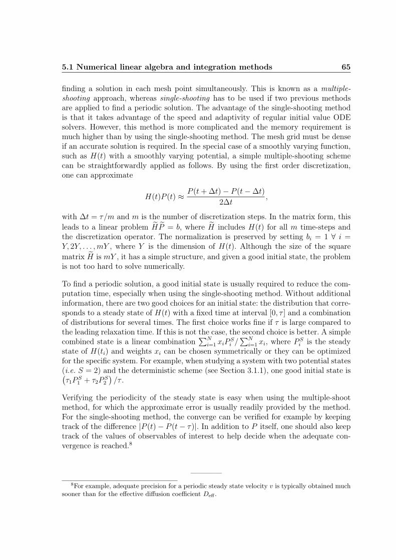
5.1 Numerical linear algebra and integration methods 65
finding a solution in each mesh point simultaneously. This is known as a multiple-shooting approach, whereas single-shooting has to be used if two previous methodsare applied to find a periodic solution. The advantage of the single-shooting methodis that it takes advantage of the speed and adaptivity of regular initial value ODEsolvers. However, this method is more complicated and the memory requirement ismuch higher than by using the single-shooting method. The mesh grid must be denseif an accurate solution is required. In the special case of a smoothly varying function,such as H(t) with a smoothly varying potential, a simple multiple-shooting schemecan be straightforwardly applied as follows. By using the first order discretization,one can approximate
H(t)P (t) ≈ P (t+∆t)− P (t−∆t)
2∆t,
with ∆t = τ/m and m is the number of discretization steps. In the matrix form, thisleads to a linear problem HP = b, where H includes H(t) for all m time-steps andthe discretization operator. The normalization is preserved by setting bi = 1 ∀ i =Y, 2Y, . . . ,mY , where Y is the dimension of H(t). Although the size of the squarematrix H is mY , it has a simple structure, and given a good initial state, the problemis not too hard to solve numerically.
To find a periodic solution, a good initial state is usually required to reduce the com-putation time, especially when using the single-shooting method. Without additionalinformation, there are two good choices for an initial state: the distribution that corre-sponds to a steady state of H(t) with a fixed time at interval [0, τ ] and a combinationof distributions for several times. The first choice works fine if τ is large compared tothe leading relaxation time. If this is not the case, the second choice is better. A simplecombined state is a linear combination
∑Ni=1 xiP
Si /∑N
i=1 xi, where P Si is the steady
state of H(ti) and weights xi can be chosen symmetrically or they can be optimizedfor the specific system. For example, when studying a system with two potential states(i.e. S = 2) and the deterministic scheme (see Section 3.1.1), one good initial state is(τ1P
S1 + τ2P
S2
)/τ .
Verifying the periodicity of the steady state is easy when using the multiple-shootmethod, for which the approximate error is usually readily provided by the method.For the single-shooting method, the converge can be verified for example by keepingtrack of the difference |P (t)− P (t− τ)|. In addition to P itself, one should also keeptrack of the values of observables of interest to help decide when the adequate con-vergence is reached.8
————8For example, adequate precision for a periodic steady state velocity v is typically obtained much
sooner than for the effective diffusion coefficient Deff .

66 Computational methods
0 100 200 300 4000
20
40
60
80
100
120
t
CP
U ti
me
ExpokitRK4−5 (a)
2 4 6 8 10 12 14 16
x 104
10−8
10−6
10−4
kP
k(t
=50
0)
(b)
Figure 5.2: Comparison of the Krylov subspace based matrix exponential method (blue line) andRunge-Kutta 4-5 method (red line) for integration of distribution P (t). (a) Computation time as afunction of the integration time t for the island model. (b) Components of the solution P (t = 500)for the RD model.
We end this Section by comparing the RK4-5 and Krylov subspace matrix exponentialmethods to solve the transient state P (t), starting from a randomized initial stateP (0). Matlab’s build-in implementation of RK4-5 is used, and for the exponentialmethod, we use Expokit9, which is also coded using MATLAB. For both methods,similar error tolerances are used, while keeping other method-dependent parametersclose to their recommended defaults. We use the reduced island model in a staticfield and the RD model in a static ratchet potential (i.e. S = 1) with L = 3. We setN = 11 for both models. In Fig. 5.2(a), the computation time is shown as a functionof the integration time t, averaged over 10 independent runs for the island model.The behavior for the RD model was found to be almost identical. As expected, thematrix exponential method is generally much faster than Runge-Kutta integrationwhen t is large. Only with small values of t, the Runge-Kutta method is slightlyfaster, because there is no need to set up a Krylov subspace. However, the accuracyof the matrix exponential method is found to be poor for large t as the numericalerror accumulates. This is demonstrated in Fig. 5.2(b) where we have plotted thesnapshot of all components of P (t = 500) in an increasing order for the RD model. Inthe Krylov subspace method, small components cannot be computed accurately, whilethe Runge-Kutta method provides accurate results for all components. Because of this,the matrix exponential method results in inaccurate values for the velocity. Therefore,we find Runge-Kutta method more suitable for solving transient and time-dependentsteady states.
9http://www.maths.uq.edu.au/expokit

5.2 Optimization 67
5.2 Optimization
The good numerical accuracy of the master equation method also makes it possibleto perform numerical optimization. In this Section, we describe methods that can beapplied to optimize scalar valued observables with respect to model parameters andsequences. This leads us to two separate and specialized fields of nonlinear constrainedoptimization of smooth functions and combinatorial optimization of cycles on graph.
5.2.1 Optimization with respect to cycles
Consider a system described by a stochastic generator H. As noted in Section 2.1.3,a nonequilibrium state results in a nonvanishing current on graph that represents thestate space. Depending on the details of the model and on the way the driving forcesare implemented, some cycles become statistically more important than the others. Weare interested in cycles that become most important with respect to a given measure.Such cycles can give important insight for example on how the transport processproceeds microscopically. To compare cycles, one needs a measure and a computationalmethod to determine the most important cycles. One type of a measure, based onthe probability of the cycle, was considered in Section 2.2.3 (see Eq. (2.8)). In thisSection, we introduce another one which is suited for very large graphs. We beginby introducing algorithms for cycle enumeration and mean cycle ratio optimization,which are both well-known problems in computational graph analysis [105]. In thefollowing, only basic knowledge of the graph theory is expected (see e.g. Ref. [15]).
Cycle enumeration
The task of finding all simple (i.e. non-intersecting) cycles of the graph is known ascycle enumeration. All known methods for this problem use a brute-force approach.For directed graphs, there are two efficient methods by Johnson and Tarjan [91], bothfrom the 1970’s. These methods are based on the standard depth-first search and usebacktracking and pruning, which significantly improve the efficiency of computationbecause there is re-counting of already found cycles. Not much progress has beenmade since these algorithms, and Johnson’s algorithm is still considered to be thefastest one with an upper time bound of O ((n+m)(c+ 1)), where m is the numberof edges, n is the number of vertices and c is the number of simple cycles [114]. Sincethe number of cycles has usually a factorial dependency on n and m, the running timeof this algorithm becomes huge for large graphs. The worst case scenario occurs whenthe graph contains very long cycles, including one or several Hamiltonian cycles.10 Insuch cases, the number of simple cycles is very large even for small graphs.
10Hamiltonian cycle is a simple cycle that includes all vertices of the graph.

68 Computational methods
Optimal cycle ratios
Consider a directed graph with n vertices and m edges. Each directed edge e is as-sociated with two real numbers: a positive or negative weight W1(e) and a positiveweight W2(e). Let us define two object functions,
ρ(C) =
∑e∈C W1(e)∑e∈C W2(e)
(5.1)
γ(C) =
∑e∈C W1(e)
|C| , (5.2)
where C is a simple cycle and |C| is the number of edges in the cycle C (i.e. cyclelength). Using these, we define two combinatorial optimization problems: the mini-mum cycle ratio (MCR) ρ∗ and the minimum cycle mean (MCM) γ∗ with
ρ∗ = minCρ(C)
γ∗ = minCγ(C),
where the minimization is performed over all simple cycles. Since the MCM problemis just a special case of the MCR problem, any algorithm that solves the latter canalso solve the first. We concentrate on the MCR problem. The need to solve this typeof problem originates from the classical tramp steamer problem, where the captain ofthe steamer wants to know what ports the steamer should visit, and in which order,in order to maximize his average daily profit. Traditionally W1 and W2 are thereforeidentified as a cost and a transit time [105].
The solution of the MCR problem can be associated with the sign changes of cycleweight computed with
∑e∈C W (e), where W is a modified weight function. To see
this, let us define a new edge weights W (e) := W1(e)−ρW2(e) where ρ is an arbitraryreal number. Using these new weights, three situations appear for a given ρ [1]:
• A negative cycle exists:∑
e∈C W (e) < 0 ⇔ ρ > ρ(C) ≥ ρ∗
• No negative cycles:∑
e∈C W (e) > 0 ⇔ ρ < ρ∗ ≤ ρ(C)
• Zero cycle:∑
e∈C W (e) = 0 ⇔ ρ∗ = ρ(C)
Starting with an arbitrary value of ρ and using a shortest path algorithm that candetect a negative cycles in the graph, and by iterating ρ, one can approach the precisevalue for which the last negative cycle disappears and thus find ρ∗. Negative cyclescan be found for example by using the Floyd-Warshall algorithm [191].

5.2 Optimization 69
Several algorithms have been proposed for an efficient numerical implementation ofthis general idea. A list and comparison of algorithms is given in Ref. [42]. It hasbeen found that Howard’s algorithm [83] is one of the fastest algorithms available[41, 42, 40]. Efficient implementation of this method can be found in the Boost C++library.11 There are two known lower bounds for the running time of this algorithm: itsrunning time is at most O(nmc), where c is the number of simple cycles, or its runningtime is at most O(n2m(max(W1) − min(W1))/ǫ), where ǫ is the required numericalprecision of the algorithm [42]. However, these are only approximations and the exactcomplexity of Howard’s method is not known. Since the second of these upper limitsfor the running time does not depend on the number of cycles, it is evident that thisproblem is much easier than the enumeration.12
Optimized cycles for nonequilibrium systems
It is evident that finding a cycle related to the largest measure via enumeration iscomputationally too expensive for all but very small graphs. There is no efficientway to find a simple cycle with a maximal (or minimal) weight using the measureof the type (2.8). Solving this problem exactly requires full enumeration, which is animpossible if the graph is large and has long cycles. Therefore we propose using ameasures of the type (5.1) and (5.2), and use them to find cycles that are importantfor the transport. Because the circulations are directed, we also reduce the number ofcycles by considering only directed graphs where the direction of the edges goes alongthe net probability flows.
We start by noting that if a system is closed and the probability is conserved, theremust also be a cycle with circulation. The situation is analogous with electric flows ina closed circuit. For a time-independent steady state, this follows from noticing thatfor every vertex, one must have 0 =
∑i [Jy,i − Ji,y] for all y. Similarly, for the periodic
time-dependent steady state P (t) = P (t+ τ) one has 0 =∫ τ
s=0
∑i [Jy,i(s)− Ji,y(s)] ds
for all y. These conditions ensure that if there are net flows in the graph, there is atleast one cycle in the directed probability flow graph.
Once the steady state distribution P S of H is found, the net currents between thestates can be computed as Ji,j = P S
i Hi,j − P Sj Hj,i ∀ i, j. If P S and H are time-
dependent, we consider their expected values integrated over a single steady statetemporal period. We then create a graph G such that if Ji,j > 0, there exists adirected edge i → j in G with a weight Ji,j. The choice W1(e) = J(e) and W2(e) = 1creates a MCM type measure in the sense ’net transition rate/edge’, and the choiceW1(e) ≡ 1 and W2(e) = 1/J(e) creates a MCR type measure in the sense ’averagenet transition rate’ for a cycle. Using the previously introduced notation, we define
11Boost C++ is an efficient peer-reviewed library of algorithms http:\\www.boost.org12This is, of course, expected, since any cycle related optimization problem can be solved exactly
by doing the full enumeration of cycles.

70 Computational methods
object functions
γ(C) =
∑e∈C J(e)
|C| (5.3)
ρ(C) =|C|∑
e∈C 1/J(e). (5.4)
These measures are always positive and have a dimension ’1/time’. Having a simplelinear form, the first measure is robust against the appearance of arbitrary smallrates, whereas the second measure rapidly drops to zero if very small weights appear.Therefore the first measure is numerically more stable, whereas the second measure isintuitively more pleasing, since there is a heavy penalty for cycles with slow net flows.Both measures rely on net currents and therefore they only work for nonequilibriumstates. Note that for irreversible transitions, such as those appearing in the TASEPmodel, the currents are directed by construction and both measures are well suitablealso in such case. When compared to the measure w(C) defined in Eq. (2.8), there aretwo differences. Firstly, the number of cycles is significantly reduced since the graph isdirected, thus making the computations much easier. Secondly, in w(C), the samplingis made over cycles (i.e. how often the cycle is realized during the process), whereas inabove measures γ(C) and ρ(C), the sampling is made over the expected probabilityflows of individual transitions, which are then combined into a cycles by using thegraph topology. Being unable to optimize the stochastic sequences using w(C), weinstead optimize the flows occurring in the corresponding master equations (whichare deterministic). These problems are fundamentally different, but according to ournumerical studies using small polymers and islands, the optimized paths typically turnout to be the same ones.
Measures (5.3) and (5.4) can be augmented with an additional weight function. For anobservable defined with an edge weight function f(e), we can take W1(e) = f(e)J(e)and W2(e) = f(e), leading to
γ(C)f =
∑e∈C f(e)J(e)
|C| (5.5)
ρ(C)f =
∑e∈C f(e)∑
e∈C 1/J(e). (5.6)
Now let us consider the case, where the function f is given by center-of-mass displace-mentsD(e) of transitions. Then the dimension of the measures become ’distance/time’and they can have negative and positive values. We call cycles with maximal ρ(C) andγ(C) dominating processes, and cycles with maximal (or minimal) ρ(C)D and γ(C)Ddominating transport processes.
Whether there is a difference between ρ and ρD, and γ and γD, depends on thedetails of the system. It may turn out, that γ and ρ only include transitions that are

5.2 Optimization 71
not responsible for directed transport, but transitions of non-transporting diffusivemotion only. Formally, this means that
∑e∈C D(e) = 0 and in that case we call the
process non-transporting, as the net transport for the cycle is zero. This is typical toratchet transport, since the object spends most of its time near the minimum of thepotential, being unable to move until the suitable state of the potential and internalstate is reached. Therefore ρD and γD carry more interesting information about thetransport, as they also take into account the displacements. If the cycle has a property∑
e∈C D(e) 6= 0, we call it a transporting process. However, it is not guaranteed thatthe dominating process is a transporting process in either case.
To study dominating transport processes, it is sometimes useful to consider a reducedsystem instead of the full one. Such situations typically arise when temporal and/orspatial states of the potential are included in the master equations, but one is onlyinterested in the internal dynamics of the transported objects (e.g. polymers andislands). Then one can sum over all non-interesting states of the master equation setto receive averaged J and D that correspond to a reduced system. For example, forthe repton model with a stochastic potential with S > 1 and L > 1, averaging over allpotential states reduces the dimension of these graphs from SL3N−1 to 3N−1. Dealingwith the reduced graphs instead of full ones, also makes the optimization of γ and ρeasier.
Graph optimization based on measures (5.3)-(5.6) is straightforward and fast, and, inprinciple, can be done for all finite discrete stochastic nonequilibrium systems. Thismethod is suitable in situations where the network is too large and complex to bestudied ’manually’ (see e.g. [35] for studies of small networks). Whether this analysisof dominating cycles is worth the effort, depends on the complexity of the systemand the importance of the internal dynamics of the objects to the transport pro-cess. For complex many-particle systems, this analysis can reveal interesting detailsof the transport, as demonstrated in Sections 6.7 and 7.4. Interest of analyzing cycleshas been also recently emerged in other fields, such as microbiology [99]. Also otherapproximate methods to determine dominant paths instead of cycles have emergedrecently [61].
————
As an example of full enumeration, we apply Johnson’s method to enumerate all di-rected cycles for a 5-atom island in a static field by using the reduced island model.In Fig. 5.3, we show the total number of cycles by their length for E = 0.04 eV.Depending on the field amplitude and direction, the total number of cycles is of order109. Considering that there are only 63 vertices and around 170 edges in the corre-sponding directed graph J , the number of cycles is already huge and the computationtakes several days. Majority of the cycles are long, and even Hamiltonian cycles are

72 Computational methods
10 20 30 40 50 6010
0
102
104
106
108
Cycle length
Cou
nt
Figure 5.3: The number of directed cycles with different lengths for the 5-atom reduced island modelwith E = 0.04 eV, T = 800 K and γ = α = 0.
common. The shape of the distribution is found to be quite similar for both islandand repton models. Because of the large number of cycles, full enumeration becomespractically impossible for systems over 100 states or even less.
5.2.2 Optimization with respect to continuous parameters
The master equation method allows fast and accurate computation of observables.This opens up an opportunity to apply optimization methods to model parameters.Although some parameters of interest might be discrete, from a computational per-spective it is usually easier to consider continuous parameters. In this Section, weconsider local optimization of scalar valued observables (denoted by the object func-tion f) computed using master equations. Since the observables are determined by themaster equation system, they are continuous and smooth with respect to the param-eters.13 We also review some of the most important optimization methods currentlyavailable. A more comprehensive listing and details of the methods can be found inmany textbooks, such as [37, 74, 128].
First we must determine the type of optimization, in which the following three aspectsare important. Firstly, since computing of observables involves solving eigenstatesand/or integration, the object function is clearly non-linear. Secondly, since we donot know the functional form of the object function, we can’t directly evaluate itsderivatives. Thirdly, parameters of the model typically have some physical constraintsthey must obey, at least upper and lower bounds. Such constraints can be linear ornon-linear. In addition to the known constraints, there are often so called ’hidden
13Although functional forms for observables cannot be generally computed, we know that theyconsists of basic arithmetic operations.

5.2 Optimization 73
constraints’ which are related to points in the feasible space where object functioncannot be evaluated, because of technical reasons. Such a situation usually occurs ifthe master equation set scales badly (i.e. becomes stiff). We are thus dealing with anonlinear constrained optimization problem.
For a nonlinear constrained optimization problem, there are two classes of methodsavailable; derivative-based and derivative-free. In the former class, derivatives of theobject function, computed either directly or approximated by finite-differences, areused to determine the optimality and search directions [74, 128]. The latter class ofmethods relies entirely on values of the object function, without using derivatives inany form. These methods do not generally require the object function to be smooth oreven continuous, and they are also often designed to tolerate noisy object functions.Majority of the research effort has been devoted to derivative-based methods, whereasderivative-free methods have become of more interest only within the last decade [37].Which of the methods works the best, depends on the problem at hand.
Problem formulation
The general constrained optimization problem is
minx∈Rn
f(x) subject to
ci(x) = 0 ∀ i ∈ E
ci(x) ≥ 0 ∀ i ∈ I, (5.7)
where E and I are sets of indices for equality and inequality constraints, respectively.Alternatively, constraints can be written in somewhat more transparent form as
~cin(x) ≤ 0, ~ceq(x) = 0, Ax ≤ bin, Aeqx = beq, L ≤ x ≤ U,
where matrices A and Aeq, and vectors bin, beq, L and U , create linear constraints,functions ~cin and ~ceq create non-linear constraints. If equality constraints are present,then depending on the size and rank of the matrix Aeq, the dimension of the state spacecan be often reduced by suitable basis transformation. The solution is approachediteratively by going through a large number of points in the feasible state-space, untilthe current iterate fulfills the optimality conditions. An iteration process requiressolving the following sub-problems: (1) how to move to the next iteration point, (2)how to fulfill constraints, and (3) testing for the optimality of the solution.
Derivative-based methods
The traditional way of optimization relies on the derivatives of the object function.Since in our case the derivatives are unavailable, they must be estimated by finitedifferences. This usually works well if the object function is a well-behaved and doesnot contain noise. Two most widely used derivative-based methods for nonlinear con-strained problems are active set and interior point methods, which differ in the wayhow the constraints are taken into account.

74 Computational methods
Moving to the next iteration, one uses either line search or trust region strategy. Inthe former, one chooses a unit vector pk and a scalar a > 0 such that xk + apk givesan improved iterate. A popular way to choose pk is the Newton method using thesecond-order Taylor series approximation mk(ǫ) := f(xk + ǫ) ≈ f(xk) + ǫT∇f(xk) +ǫT∇2f(xk)ǫ/2. For a positive-definite second derivative, the Newton direction is foundby solving mk(p) = 0.14 Instead of the pure Newton direction, computationally lessheavy Quasi-Newton direction is typically applied, where instead of a true Hessian, anapproximation is used and updated iteratively.15 Once the direction has been fixed,the step distance a can be found by solving a one-dimensional minimization problemmina>0 f(xk + apk).
In the trust region strategy, the information gathered about f is used to construct asimple model function fk which mimics f near the current point xk. The region wherefk is considered a good approximation of f , is the trust region. Within this region,the candidate step pk is found by solving the subproblem minpk fk(xk + pk), which ismuch easier for fk than f itself.16 During the optimization, the trust region can beenlarged or shrunk as needed.
The local optimality of the solution can be determined from the first and secondderivatives. However, most modern optimization methods are based on the so-calledKarush-Kuhn-Tucker (KKT) conditions, which give first-order necessary optimalityconditions for the Lagrangian function L(x, γ) = f(x)−∑i γici(x), where γi’s are theLagrange multipliers. The KKT approach to nonlinear optimization generalizes themethod of Lagrange multipliers, which allows only equality constraints.
Active set method
Active set methods are based on the observation that, in general, it is much simpler tosolve equality-constrained problems than to deal with inequalities. The conventionalactive set approach is divided into two phases; first f is ignored while a feasible point isfound for the equality constraints, next f is minimized while feasibility is maintained.One starts by making a guess of the setW of constraints, that are satisfied as equalitiesat an optimal point. Using the Lagrangian, one then solves a problem in which theconstraints in the active set W are imposed as equalities, and the constraints not in Ware ignored. Then, one checks whether the resulting point satisfies the KKT conditionsusing Lagrangian multipliers. If so, a local optimum has been found, otherwise a newchoice for the active set is made, and the process is repeated. The path of points neverleaves the feasible region, but it can hit its boundaries. Particularly, active set strategy
14For non positive-definite case, the definition of pk is modified to make it satisfy the descentcondition while retaining the second-order information [128].
15One chooses the new Hessian approximation Bk+1 which mimics the property ∇2fk(xk+1−xk) ≈∇fk+1−∇fk. The most popular formula updating B is a Broyden-Fletcher-Goldfarb-Shanno (BFGS)method.
16Unlike in the line search methods, the direction and distance are solved simultaneously.

5.2 Optimization 75
is applied within Sequential Quadratic Programming (SQP) methods, which convertthe nonlinear optimization problem into linear-constrained quadratic sub-problems.A detailed description of the SQP method can be found in Ref. [128].
Interior point method
In interior point method, the problem (5.7) is reformulated in the form
minx,s
[f(x)− µ
∑
i
ln(si)
]subject to
~ceq(x) = 0
~cin(x)− ~s = 0
~s > 0
,
where the scalar µ is positive. The components si of the vector ~s are called slackvariables. This new object function has smooth barriers at the limits of the feasibleregion. The path of generated points never leaves the feasible region and cannot hitits boundaries. This type of penalty barrier approach consists of finding approximatesolutions to the barrier problem and reducing µ towards zero, from which the solutionfor the original problem is recovered. Further details can be found in Ref. [128].
Interior point and SQP methods are considered to be very powerful algorithms forlarge-scale nonlinear optimization problems. Active set approach typically requires alarger number of iteration steps, while a single iteration is computationally inexpen-sive. Interior point approach requires a smaller number of more expensive steps. Forvery large problems, interior point methods are often more efficient. However, whena good estimate of the solution is available (a ’warm start’), the active set approachmay converge rapidly.
Derivative-free methods
The methods designed not to rely on derivatives or their approximations, are calledderivative-free or direct search methods. The performance of derivative-free meth-ods is not usually comparable to that of derivative-based methods in accuracy or innumber of parameters to be optimized. The stopping criteria are also a challenge inabsence of derivatives and when f includes noise. When compared to the derivative-based methods, derivative-free methods are reasonably straightforward to implementfor any model and therefore they can be used as the method of first recourse. Therequirements from a user are minimal and algorithms themselves require setting onlya few parameters [37].
Here we only consider the most basic derivative-free method known as the patternsearch method (also known as as the directional direct-search method). Pattern searchmethods are characterized by a series of exploratory moves that consider the behav-ior of the object function at a pattern of points. The exploratory moves consist of

76 Computational methods
a systematic strategy for visiting the points in the lattice in the immediate vicinityof the current iterate point. This is called polling. There are several different choicesfor creating a search mesh and performing the polling. For example, the mesh can becreated by using the generalized pattern (GP), the generating set (GS) and the meshadaptive direct (MADS) algorithm. Put in short, the GP method uses axis directedbasis vectors, whereas GS can take into account the linear constraints in search direc-tions. MADS is a further generalization of GS type algorithms by allowing even moreflexible search directions. The number of basis vectors is either N +1 or 2N , where Nis the number of variables to be optimized. Polling can be complete or partial, whichmeans that as soon as a better value for f is found, polling is stopped. The searchgrid is typically enlarged or shrunk during the run. Iteration is stopped when thetolerance for the object function or the minimum grid size is met. Constraints can betaken into account by adding penalty for constraint violations or using a hard barrier.However, handling of constraints is typically crude when compared against interiorpoint and active set approaches.17 Additional details of different methods and theorycan be found in Ref. [37]. For a listing of freely available derivative-free optimizationsoftware see Ref. [151].
————
To compare active set, interior point and pattern search optimization methods, wehave computed the optimal charge distribution and the optimal temporal flashingperiod for the non-homogeneous RD model, such that the velocity function v(q, τ) :=v(q1, q2, . . . , qN , τ) is maximized and minimized. Non-zero velocity is generated by astochastically flashing ratchet with S = 2, L = 3 and Vmax = 1 (this potential isdiscussed in more details in Chapter 6). This constrained optimization problem is arather complicated one in the sense, that there are several local maxima and minimaand the parameter space includes two types of variables (charges and temporal period).There are N +1 variables to optimize. We consider a situation where the total chargeis limited by an equality
∑i qi = Q or an inequality
∑i qi ≤ Q. The temporal period
τ has only a lower bound τ = 0, but for better numerical stability, we set limits10−4 < τ < 106 (these are the ’hidden constraints’ discussed previously). We useMATLAB implementations for all three methods (active set method is implementedin the SQP algorithm).18 Randomized near-uniform (i.e. qi ≈ 1 ∀ i) initial chargedistributions are used. In this test, we set N = 9, which already requires several hoursof computing.
Solving the problem several times using different methods, it becomes evident that the
17Constrained derivative-free optimization is still a subject of intense research and most derivative-free methods are currently designed only for unconstrained problems.
18All three methods are included in Optimization Toolbox (version 5.0) and the Global Optimiza-tion Toolbox (version 3.0).

5.2 Optimization 77
0 50 100 150 200−2
−1.5
−1
−0.5
0
0.5
1x 10
−5
Iteration
v(q
,τ)
Pattern searchInterior−pointSQP
(a)
20 40 60 80 100 120
−12
−10
−8
−6
−4
−2
0x 10
−4
Iteration
−v(q
,τ)
(b)
Figure 5.4: Example optimization runs of (a) the inverse and (b) the main velocity for the RDmodel, with N = 9 in a stochastic flashing ratchet, with S = 2, L = 3 and Vmax = 1. The sameinitial state is used for all three methods.
global maxima and minima are found at the boundary of the feasible space, i.e. we mayuse condition
∑Ni=1 qi = Q. The problem involving the inequality is more complicated
to solve and all three methods usually fail to find a good solution, especially SQP. Thisemphasizes the importance of a proper problem formulation before the optimization.In Fig. 5.4, a typical convergence behavior of the methods is shown. For the patternsearch method, satisfactory results were reached using GS pattern with 2N basisvectors and a complete polling. Using other patterns or only N+1 basis vectors, oftenfails or leads to slower convergence. The velocity is shown as a function of the iterationnumber when optimizing the velocity in both (a) inverse and (b) main direction (thedifference between these are explained in Section 6.3). The latter optimization turnsout to be much more complicated, because of several very deep local minima createdby accumulation of the charge on a single repton (this is expected, because of theexponential form of the rates). In Table 5.2, the computational times, the numberof iterations and the number of function evaluations are shown as a median for 10independent runs.
There is no explicit winner between the methods. The convergence of the patternsearch method is rapid at the beginning, but then slows down. It fails to find theglobal minimum for the inverse direction, but finds it for the main direction, althoughwith a slight violation of constraints. Choosing the proper polling pattern and type isessential, which requires testing many combinations. This method also needs lots offunction evaluations. The SQP method converges well and reliably for both problemsand requires less function evaluations. It is also most robust against changes of theinitial state. However, it fails badly when using inequality constraints. The interiorpoint method is reliable, but converges more slowly and requires lots of evaluations.As expected, both the SQP and the interior point method respect constraints well.

78 Computational methods
Table 5.2: Median results over 10 independent optimization runs with random initial states, usingthe interior point (IP), the pattern search (PS) and the SQP method.
Inverse direction Main directionIP PS SQP IP PS SQP
Time (10−2) 185 112 108 77 116 63Iterations 232 139 132 108 209 82
Evaluations 2790 1580 1645 1223 1523 931Value (104) 0.209 0.204 0.209 11.43 12.82 11.43
5.3 Monte Carlo method
Monte Carlo methods form the largest and the most important class of numericalmethods used for solving statistical physics problems [126]. The idea of the method isnot to compute probability distributions directly, but approximate those by averagingover a large number of sampled paths, that are generated using random numbers.The law of large numbers ensures that the expected values of observables approachthose computed directly by solving master equations. The Monte Carlo method canbe used for any type of systems and all observables. For discrete-time systems, clas-sical Metropolis algorithm is often used to create the dynamics for simulations. Forcontinuous-time systems a popular continuous-time Monte Carlo method was intro-duced by Bortz et al. in 1975 [21], and since then, several improvements have beenmade [28]. This method is known as the kinetic Monte Carlo or N-fold algorithm andit works by sampling sequences and waiting times separately (the theory behind thiswas discussed in Section 2.2.3).
In the N-fold algorithm, transitions (reactions) are divided in different classes accord-ing to their rate. During the simulation, one keeps up a list of all available reactions forthe current state of the system. Time-steps and reactions occur randomly such thatthey correspond to the dynamics of the master equations. In this work, we implementthe kinetic Monte Carlo method using the following algorithm (see Ref. [88]):
1. Initialization. Generate an initial state, create reaction lists and set elapsedtime to zero.
2. Time-step generation. Increase the time by generating an exponentially dis-tributed time-step using the total escape rate.
3. Picking a reaction. Randomly pick a reaction from the list and test checkwhether it is allowed. If the reaction is not allowed, go to step 6.
4. Allowed reaction. Make the transition into a new state and remove the reac-tion from the list.

5.3 Monte Carlo method 79
5. Adding new reactions. Add new reactions that became available. Go to step7.
6. Forbidden reaction. Remove the reaction from the list.
7. Continuation. If the ending criterion is met, end simulation. Otherwise go tostep 2.
The only model-dependent parts of the algorithm are the initial state generation,adding and checking reactions. In our implementation, the reaction list is createdusing a linked list.19 Technical details about each step can be found in Ref. [88].
The major downside of the Monte Carlo method is the low accuracy. Accurate re-sults require lots of computation time and careful monitoring to ensure validity of theresults. One must choose the number of independent iterations and simulation timecarefully to get correct (steady state) sampling, while simultaneously trying to keepcomputational time as small as possible. If low quality or unsuitable random numbergenerator is used, bad sampling may occur and the results will be unreliable. Com-puting certain types of observables, such as relaxation times, may be complicated.Since the data computed via Monte Carlo method is noisy, post-processing, includingsmoothing and (polynomial) fitting, is usually needed to extract information, such asmaximum and minimum values and numerical derivatives.
Although the Monte Carlo method is straightforward, the efficient implementationfor a specific model can be tricky. To get accurate results, finding and checking thereactions cannot be too time consuming, hence the usefulness of the method dependson the complexity of the model. If the model is very complicated, e.g. the interactionsare long-ranged and there are lots of reactions, manipulating the data structures canbecome the bottleneck for the simulations.
Adding new reactions in the island model
The core part of the kinetic Monte Carlo algorithm is adding reactions to the reactionlist. This is typically the most time-consuming part of the algorithm. For the islandmodel, the search for new reaction takes place in the neighborhood of the hoppingatom shown in Fig. 5.5. Moving a single atom affects 16 neighbor lattice sites andtheir atoms, by either allowing or blocking moves and/or changing energy barriers.For those sites numbered with 1-6, transitions can be created or blocked and thebarriers changed. For sites numbered with 7-16, only the barriers might be changedfor some of the transitions. It is easy to see, that increasing the interaction lengthwould greatly increase the number of affected neighbor atoms, thus increasing the
19We also implemented a binary tree list, which, however, in most situations turned out to be lessefficient for the island model.

80 Computational methods
12 3
456
78
9 1011
1213
141516
Figure 5.5: The local neighborhood that has to be checked in the kinetic Monte Carlo simulationafter the transition of a single atom (sphere at the middle). For sites marked with gray, only theenergy barriers of the already existing reactions can be affected and for the rest, new reactions arecreated or old ones disabled.
computational cost of the simulation. More technical details of the kinetic MonteCarlo simulations for the island model can be found in Ref. [79].

6 Results for the repton model
In this Chapter, we present selected results from Articles I and II for the repton modelintroduced in Section 3.3. Also some additional results not found in the Articles arepresented in Section 6.2. The results shown in this Chapter are computed using thenumerical master equation method. Since the repton model includes a large numberof parameters, some of them must be fixed, primarily those that have a minimalqualitative impact on the results. In addition to the repton count N , other parametersin the models have the following interpretations:
• The environment ↔ the potential V (x, t) = V (x+ L, t+ τ)
• The medium ↔ tube deformation Ω (0 for RD, 1 for FM)
• The polymer internal fine-structure ↔ charges q1, . . . , qN
The single most important parameter is the temporal period τ of the potential, whichis also easily controlled in experimental set-ups. The parameter Ω models the porosityand viscosity of the medium by either restricting the polymer strictly into the reptationtube (Ω = 0) or not (Ω = 1). We set L = 3 for the spatial period (with the onlyexception made in Section 6.2), and use two potential states (i.e. S = 2). These choicesallow both maximal N/L ratio and keeps matrix sizes feasible for the numerical matrixequation method. With these choices, a flashing ratchet is defined by setting Von(1) =0, Von(2) = Vmax/2, Von(3) = Vmax, and Voff(x) = 0 ∀x, and the traveling potentialis defined by V1(1) = V2(2) = Vmax and zero for V1(2), V1(3), V2(1) and V2(3). Thesepotentials are illustrated in Fig. 6.1. The maximum potential strength Vmax has only asmall effect on the results and is set to unity if not mentioned otherwise. The directionof the potentials is set up in such way, that the expected long-time ’main velocity’is positive and the long-time ’inverse velocity’ (if present) is negative.1 Potentials arechanging in time in stochastic, deterministic or smoothly varying manner, as explainedin Section 3.1.
1Note that in Article I the main velocity has a negative sign and the inverse velocity is positive,whereas in Article II is it other way around. Here we have made a compromise by plotting −v and−d in some figures.
81

82 Results for the repton model
1 2 3 4 5 6 7
0
0.2
0.4
0.6
0.8
1
V/V
max
1 2 3 4 5 6 7
0
0.2
0.4
0.6
0.8
1
V/V
max
lattice site
1 2 3 4 5 6 7
0
0.2
0.4
0.6
0.8
1
1 2 3 4 5 6 7
0
0.2
0.4
0.6
0.8
1
lattice site
on
off
1
2
Figure 6.1: Sketch of a flashing non-symmetric ratchet (left columns) and the traveling symmetricratchet (right columns) for L = 3 (two period lengths shown). In these potentials, the chosen mainvelocity direction is on the left.
6.1 Choosing the rates
As discussed in Section 2.2.2, the selection of rates is important for the nonequilibriumsystems. To demonstrate this, in Fig. 6.2 we have plotted the steady state velocityand diffusion coefficient of the 8-repton RD polymer in a stochastic flashing ratchetand traveling potential. Although all three curves for flashing and traveling potentialsshare a similar shape, the scales are different and large differences can be seen in thelimit where the temporal period τ → 0. Only exponential (in a flashing ratchet) andMetropolis (in a traveling potential) dynamics lead to zero drift in this limit, whichis a physically expected situation (see Section 3.1.3) and is also consistent with thesingle Brownian particle models [12, 109, 155]. Therefore we choose these rates for therepton model.
6.2 Relaxation in a flashing ratchet
First we study the relaxation process of the repton model in a flashing ratchet potentialdepicted in the left column of Fig. 6.1. In Fig. 6.3, we have plotted the time-dependentvelocities of 10-repton polymers during their relaxation, when the potential state isswitched at t = 0 and the polymer is in equilibrium at t < 0 with zero averagevelocity v(t < 0) = 0. In Fig. 6.3(a), the uniformly charged RD and FM polymers arecompared (the total charge Q = 10). The time-dependent total displacement of the

6.2 Relaxation in a flashing ratchet 83
−2 0 2 4 60
5
10
15
104
v
−2 0 2 4 6
6
8
10
103
Deff
ln(τ)
−2 0 2 4 60
2
4
6
−2 0 2 4 64
6
8
10
ln(τ)
Figure 6.2: The effect of the jump rate scheme. The velocity and the diffusion coefficient of the8-repton RD polymer as a function of the temporal period τ in a stochastic flashing ratchet withL = 3 and Vmax = 1 (left) and the traveling potential (right), with exponential (blue dash-dottedlines), Metropolis (black solid lines), and Kawasaki (red dashed lines) rates.
center-of-mass,
d(t) =
∫ t
0
[von→off(s) + voff→on(s)] ds,
is shown in the inset figure. The asymptotic value d := d(∞) was previously dis-cussed in Section 3.1.3. For rigid objects without internal configurations and withoutdeformable shapes, clearly von→off(t) ≡ 0 because there is no directed center-of-massmotion for t > 0. However, for other objects there is a non-zero relaxation time relatedto the internal configurations of the object, hence von→off(t) is generally non-zero. Wecall this relaxation a rebound effect. For the repton model in a flashing ratchet, it isfound that von→off(t) has an opposite sign compared to voff→on(t), which is consideredas the main velocity. As noted in the beginning of this Chapter, we have chosen thedirections such that voff→on(t) > 0 is expected.
The rebound effect is much stronger for the RD polymers, and with combined effectof the weaker main velocity, causes the current inversion, where the long-time velocityis negative (i.e. the polymer travels ’backwards’). For the FM model, the reboundeffect is generally too weak to allow current inversion. One can also notice the muchfaster relaxation of the FM model. In Fig. 6.3(b) the effect of non-uniform chargedistribution is shown for the RD model with total charge Q = 6.2 All the charge put
2To study polymers with a single charged repton, the total charge cannot be too large, otherwisethe master equation set becomes stiff.

84 Results for the repton model
0 2 4 6 8 10
−4
−2
0
2
4
6
8
10
12
x 10−3
t
−v(t
)
on → off (RD)
off → on (RD)
on → off (FM)
off → on (FM)
0 50 100−0.015
−0.01
−0.005
0
0.005
t
−d(t
)
(a)
0 1 2 3 4 5 6 7 8
0
1
2
3
4
5
6
x 10−3
0 1 2 3 4 5 6 7 8
−0.05
0
0.05
0.1
0.15
0.2
0.25
t
−v(t
)
off → on (c)
on → off (c)
on → off
off → on
off → on (1)
off → on (2)0 50 100 150
−0.1
−0.05
0
t
−d(t
)
(b)
Figure 6.3: The velocity after the potential is switched at t = 0 for a deterministic flashing ratchetat the large τ limit. (a) RD (red lines) and FM (blue lines) polymers with homogeneous chargedistributions and a total charge Q = 10. (b) RD polymers using a middle-centered (blue lines),homogeneous (red lines), the first repton (black line) and the second repton (green line) chargedistributions with Q = 6. Note the different y-axis used for the black and green lines, because of thelarge scale difference. In both figures N = 10, L = 3 and Vmax = 1. The integrated total displacementis shown in inset figures.
into a single repton leads to a large drift towards positive direction, since the reboundeffect is non-existing. This is because all internal states have an equal probability,hence there cannot be net velocity when the potential is turned off. Although thehead-charged polymer (repton 1 or 6 in Fig. 4.1) is faster shortly after the potential isturned on, the polymer with the second repton charged (i.e. repton 2 or 5 in Fig. 4.1)produces a larger total displacement due to the longer relaxation process. On theother hand, the rebound effect can be maximized by concentrating the charge on themiddle reptons. In this example, total charge was distributed according to percent-ages [0, 5, 10, 15, 20, 20, 15, 10, 5, 0] for q1, . . . , q10. The reason for such a distributionbecomes evident later in Section 6.4.
In Fig. 6.4, similar data is shown for the case L = 6 so, that when the potential isturned on, its profile remains identical to the case L = 3, but the scale is doubled(i.e. lengths of the slopes are 4 and 2 steps). Now the rebound effect is not enoughto cause current inversion for neither RD nor FM polymers. Despite the stronger re-bound effect, using the middle-centered charge distribution actually leads to increasedvelocity in the main direction. This is caused by the very slowly decaying velocity intothe main direction.
Next we take a closer look at the travel distance d(t) of the center-of-mass during asingle, very large time-period τ of a flashing ratchet. The results for (a) L = 3 and(b) L = 6 are shown in Fig. 6.5. For N = 1, 2, there are no bulk-reptons, so the meantravel distances of RD and FM polymers may differ for N ≥ 3 only. For the L = 3, thecalculation reveals that for long RD polymers (N > 5, a ’critical length’) the rebound

6.2 Relaxation in a flashing ratchet 85
0 10 20 30 40 50
−0.02
−0.01
0
0.01
0.02
t
−v(t
)
on → off (RD)
off → on (RD)
on → off (FM)
off → on (FM)
off → on (RD c)
off → on (RD c)0 100 200 300
−0.2
−0.1
0
t
−d(t
)
Figure 6.4: The velocity after the ratchet potential is switched at t = 0 for a deterministic flashingratchet at the large τ limit. Blue and red lines are for the homogeneously charged RD and FMpolymers, and black lines for the middle-centered charged RD polymer. The data is for N = 10,L = 6, Vmax = 1 and Q = 10.
effect wins (i.e. d < 0) and the polymer starts traveling backwards, while the singleparticle and all FM polymers are traveling to the expected positive main direction.The rebound effect is also present in FM polymers, but it is not strong enough toreverse the direction of the velocity.
For the case L = 6, polymers up to 11 reptons can be treated with exact numerics,whereas time-dependent DMRG is used for larger ones. The asymptotic limit d(∞)can be reach only with the exact numerics. The results for DMRG are limited up tod(200) because of the high computational cost.3 Time-steps of ∆t = 0.05 . . . 0.07 anderror tolerance 10−9 were used. Unfortunately, the velocity is a very slowly decayingfunction for the ’off-on’ process and a notable difference between d(200) and d(∞)remain. From the behavior of d(t), one can however assume that d(t = ∞) remainsalways smaller than d(t) with finite values of t and large RD polymers. Based onthis and our Monte Carlo simulations for large τ ’s (data not presented here), we mayconclude that the current inversion does not occur for uniformly charged RD polymersin the case L = 6. Similar results were also found for L = 4 and L = 5, hence the caseL = 3 seems a special case for the RD model. Using non-uniform charge distribution,d becomes closer to zero, but still remains positive for L = 6. However, since optimalcharge distributions are not known for large RD polymers and d approaches zeroas the polymer gets larger, current inversion still cannot be completely ruled outfor very large polymers N > 25 with optimal charge configurations. One could alsotry to reinforce the rebound effect by adding longer-range interactions (e.g. stiffness)between reptons which might also lead to current inversion for L > 3.
3These results required already more than a month of uninterrupted parallel computing to finish.

86 Results for the repton model
2 4 6 8 10
−0.015
−0.01
−0.005
0
0.005
0.01
N
−d(t
)
30 (RD)
100 (RD)
300 (RD)
∞ (RD)
30 (FM)
100 (FM)
300 (FM)
∞ (FM)
(a)
5 10 15 20 25
−0.14
−0.12
−0.1
−0.08
−0.06
−0.04
−0.02
0
N
−d(t
)
50 (RD)
100 (RD)
150 (RD)
200 (RD)
∞ (RD)
50 (FM)
100 (FM)
150 (FM)
200 (FM)
∞ (FM)
(b)
Figure 6.5: (a) Expected travel distances d(t) of the RD polymers (blue lines) and FM polymers(red lines) in a deterministic flashing ratchet (L = 3 and Vmax = 1) as a function of the polymerlength in single time-period at asymptotic limit (i.e. the steady state is reached before the switching).Different t’s are indicated with different marker types. (b) The similar data for L = 6. Polymers upto N = 11 were computed with exact numerics and larger ones with time-dependent DMRG. Theasymptotic limit d(t = ∞) is reached only using exact numerics.

6.3 Velocity and diffusion in the steady state 87
6.3 Velocity and diffusion in the steady state
6.3.1 Flashing ratchet
We fix the symmetry parameter x = τoff/τ to x = 1/4, 1/2, 3/4 and examine theτ dependence of the steady state velocity v and the Peclet number Pe = |v|/Deff instochastic potentials. The results in Fig. 6.6 reveal a complex behavior of the velocity.The overall form of the curves is as expected: the velocity and the Peclet numberhave some (local) maxima around ln (τ) ≈ 0. For small τ , the single particle remainsthe fastest in all cases excluding x = 1/2 for FM polymers, where it is the slowestone. However, as τ gets larger, longer polymers eventually become faster, which iscaused by their longer relaxation time (short polymers have already reached theirsteady state). This can be clearly seen from Figs. 6.6(b) and (c), but it also takesplace in figure (a) to some extent. Similar behavior of coupled particles being fasterthan single ones and also having current inversions were also reported in Ref. [100].Although the relaxation times are quite different, the maxima of the velocity fall closeto ln (τ) ≈ 1 for all polymer lengths and the position of the maximum Peclet numberis almost constant. The velocity sign change occurs for some polymers when τ is verylarge or when τ is small and x > 1/2.
The behavior of the Peclet number is very clear and similar in every case: the largerthe polymer, the larger the Peclet number. Thus the transport of longer polymers ismore coherent than that of shorter ones. Similar behavior was found in a continuummodel consisting of elastically coupled Brownian particles [187]. By comparing thevalues of the Peclet number between polymer types, we see no significant differencesbetween the curves. There is a slight difference for large values of τ , where the Pecletnumber remains larger for FM polymers. This holds with every choice of parameters,excluding the possible current inversion points (e.g. the interval ln (τ) = −1 . . . 0 inFig. 6.6(c)).
Next we compare the differences of the three potential time-dependency schemes(stochastic, deterministic and smoothly varying) in a flashing ratchet potential, forwhich the differences are more distinct. In Fig. 6.7 we have plotted v and the Pecletnumber of N = 5 and N = 9 (similar behavior is observed for other values of N) RDand FM polymers as a function of τ for all three time-dependency schemes. Some cleardifferences between the schemes can be seen. The maxima for the velocity and thePeclet numbers are reached for smaller τ for the stochastic scheme than for two others.The deterministic scheme has the largest v and the smoothly varying the smallest,and the same goes for Pe. However, this order changes for the inverse velocity, wheredeterministic and smoothly varying schemes are equally good. The time-dependencyscheme turns out to have an effect on the current inversion phenomena, since thesmoothly varying scheme is able to invert all RD polymers with N > 2, whereas

88 Results for the repton model
−0.6
−0.4
−0.2
0
−10
4v
00.010.02
Pe
−0.8
−0.4
0
−10
4v
00.010.02
Pe
−3 −2 −1 0 1 2 3 4 5−0.4
0
0.4
0.8
−10
4v
ln(τ )
00.0050.01
Pe
−1.2
−0.8
−0.4
000.010.02
−0.8
−0.4
000.010.02
−3 −2 −1 0 1 2 3 4 5−0.8−0.400.40.8
ln(τ )
00.0050.01
(a)
(b)
(c)
Figure 6.6: Velocity and Peclet numbers of the RD polymers (left column) and FM polymers (rightcolumn) in a flashing ratchet (L = 3, Vmax = 1) with N = 1 (solid black), N = 3 (dash), N = 5(dot), N = 7 (dash-dot), N = 9 (solid blue). The value of the symmetry parameter x = τoff/τ is (a)x = 1/4, (b) x = 1/2 and (c) x = 3/4.

6.3 Velocity and diffusion in the steady state 89
0 2 4 60
2
4
6
104
v
0 2 4 60
1
2
3
ln(τ)
102
Pe
0 2 4 60
0.5
1
1.5
0 2 4 60
1
2
3
ln(τ)
Figure 6.7: Velocity and Peclet number for 5 (blue lines) and 9-repton (black lines) RD (left) andFM polymers (right), for deterministic (solid lines), smoothly varying (dashed lines), and stochastic(dash-dotted lines) schemes.
stochastic and deterministic only those with N > 5. Despite this, the differencesbetween deterministic and smoothly varying are small (deterministic being slightly’better’).
6.3.2 Traveling potential
Next we study transport in the stochastic traveling potential depicted in the rightcolumn of Fig. 6.8. For this potential the symmetry parameter is x = τ1/τ . A Similarvelocity and diffusion behavior as previously reported in Ref. [109, 26] for a singleparticle is expected. In Fig. 6.8, we show v as a function of x with three different τ ’s(Fig. 6.8(a)-(c)): τ → 0, ln (τ) = 3 and ln (τ) = 7. The behavior for the single particleis as expected; the velocity is antisymmetric with respect to x = 1/2 and goes to zeroat x = 0, 1/2, 1. With longer polymers the velocity changes sign non-trivially forlarge τ (Fig. 6.8(c)) for both polymer types. This result is unexpected. An example ofthe behavior of the diffusion coefficient is shown in Fig. 6.8(d) for N = 9 and differentτ ’s. Deff always reaches its maximum at x = 1/2 and decreases as the system goes toa static potential state at x = 0 and 1.
Next we fix x = 1/4 and examine the τ dependence in detail. In Fig. 6.9, we haveplotted v and the Peclet number for ln (τ) = −4 . . . 7.5. As N > 2, current inversionscan be seen around ln (τ) ≈ 2 for both polymer types. As before, the single particleremains the fastest for small τ , but eventually the velocity curves begin to intersect

90 Results for the repton model
−5
0
5
103
v
0 0.2 0.4 0.6 0.8 16
7
8
x
103
Deff
−1
0
1
103
v
−4−2
024
105
v
−5
0
5
0 0.2 0.4 0.6 0.8 1
25
30
35
40
x
−1
0
1
−5
0
5
(a)
(d)
(b)
(c)
Figure 6.8: Velocity and Peclet numbers of the RD polymers (left column) and FM polymers (rightcolumn) in the traveling potentials (L = 3, Vmax = 1). (a-c): velocity as a function of the symmetryparameter x = τ1/τ with τ → 0 (a), τ = exp (3) (b) and τ = exp (7) (c) with N = 1 (solid black),N = 3 (dash), N = 5 (dot), N = 7 (dash-dot), N = 9 (solid blue). (d): the effective diffusioncoefficient for N = 9 with τ → 0 (solid), τ = exp (3) (dash) and τ = exp (7) (dot).

6.3 Velocity and diffusion in the steady state 91
0
2
4
6
103
v
1 3 5 7 911
−1
0
1
104
v
N
−4 −2 0 2 4 60
2
4
6
102
Pe
ln(τ )
1 3 5 7 911−2
−1
0
104
v min
N
0
2
4
6
1 3 5 7 9110123
104
v
N
−4 −2 0 2 4 60
2
4
6
ln(τ )
1 3 5 7 911
−2
−1
0
104
v min
N
(a)
(b)
Figure 6.9: Velocity and Peclet numbers of the RD polymers (left column) and FM polymers (rightcolumn) in the traveling potential (L = 3, Vmax = 1) as a function of the mean time-period τ withthe symmetry parameter x = τ1/τ and N = 1 (solid black), N = 3 (dash), N = 5 (dot), N = 7(dash-dot) and N = 9 (solid blue). For the left inset of (a) ln (τ) = 2.85 and ln (τ) = 2.05 for theright inset.
as τ gets larger and the single particle is not always the fastest (see e.g. the N = 3FM polymer in Fig. 6.9(a), right column). The behavior of the Peclet number is asbefore: Longer polymers have more coherent transport, excluding the possible currentinversion points and their neighborhood. With small values of τ , the Peclet number isalso the same for both polymer types, but because of unequal velocities for moderateand large values of τ , also differences exist.
The insets of Fig. 6.9 show the velocity as a function of N = 1 . . . 11 in detail. We havechosen ln (τ) = 2.85 for RD polymers and ln (τ) = 2.05 for FM polymers. With thesechoices, the current inversion occurs between N = 6 and 7 for both models. In theinsets of Fig. 6.9(b) we have plotted the overall velocity minimal values in the intervalln (τ) = −4 . . . 7.5 as a function of N . The distinction between the polymer typesis very clear. FM polymers travel increasingly fast backwards whereas RD polymerseventually stop moving as N gets larger. The current inversion of the RD polymersN ≥ 10 would require a smaller fixed x.
The magnitude of the velocity, typically between 10−5 and 10−3, is comparable withthe velocity caused by a flashing ratchet. The Peclet number values of the polymermotion remain small (≪ 0.1) for both potential types, indicating very low coherenceof transport.

92 Results for the repton model
6.4 Non-uniform charge distributions
We now consider non-uniform charge distributions where the charges of the reptonsdiffer. As already seen for the relaxation studies, changing the charge distributionhas a dramatic effect on the velocity. To set up the optimization problem, we defineconstraints
∑Ni=1 qi = Q, qi ≥ 0 and τ ≥ 0. The objective function is the velocity
v(q1, q2, . . . , qN , τ). Some additional technical details and comparison of methods werediscussed in Section 5.2.2.
Using the SQP method, extensive computations were carried out to find the chargeconfigurations with the largest possible velocity in main (forward) and inverse (back-ward) transport directions and Pe for various polymers and parameters. It was foundthat changes in the velocity are so large that one can safely limit to maximizing valone, since in this case Pe is dominated by the velocity. In the following, some ofthe optimization results are presented for the 8-repton polymers with Q = 8 in thestochastic potentials with Vmax = 1 and L = 3. The data for the basic model withan uniform charge distribution (i.e. qi = 1 ∀ i) is also shown for comparison. Notethat since reptons are equal in the sense that their charge is allowed to vary between[0, Q], a non-symmetric distribution is equal with its mirror-symmetric counterpartwith respect the center bond (or repton, if N is odd). In the figures, only one ofsuch distributions is shown. For symmetric charge configurations, such as uniformand middle-centered, the solution is unique.
In Fig. 6.10, the properties of the RD polymer in a flashing ratchet are plotted as afunction of τ with configurations that give maximum velocities in positive (main) andnegative (inverse) directions, and the corresponding optimization results are calledeither positive or negative. We found that the velocity in the positive direction isalways maximized by putting all charge near either of the heads, but charging thehead reptons does not necessarily lead to the largest current. This holds for bothRD and FM polymers for all studied polymer lengths up to N = 13 at least. Inthis situation, only one repton feels the potential and very large transition rates aregenerated by the exponential function. This one repton then forces the whole polymerto advance. As discussed in Section 6.2, there is no rebound effect when only onerepton is charged.
The optimal charge distributions in the negative direction are more interesting, sinceno large accumulation of the charge is seen, and the charge is distributed over severalreptons. A symmetric distribution means that neither of the heads is leading andthe heads are forced to compete with each other. This would be very inefficient inconstant-field transport. Depending on the value of Vmax, other slightly different localoptimal distributions are found. In Section 6.2, it was demonstrated that the reboundeffect is strong for the RD polymers with a middle-centered charge distribution.

6.4 Non-uniform charge distributions 93
−2 0 2 4 60
1
2
3
104
v
−2 0 2 4 6
6
8
10
103
Deff
−2 0 2 4 60
1
2
3
ln(τ)
102
Pe
1 2 3 4 5 6 7 80
2
4
6
8
i
q i
v/10
Pe/10
Figure 6.10: Velocity, diffusion coefficient and Peclet number for the 8-repton RD polymer in aflashing ratchet with uniform (blue dash-dotted lines), negatively optimized (red dashed lines), andpositively optimized (black solid lines) charge distributions as a function of the temporal period τ .The histogram shows the charge distribution along the polymer for each case in the same order. Inthe leftmost figures v and Pe for the positively optimized case have been scaled by an additionalfactor 1/10.

94 Results for the repton model
−2 0 2 4 6−2
0246
104
v
−2 0 2 4 6
2
4
6
103
Deff
−2 0 2 4 60
5
10
ln(τ)
102
Pe
1 2 3 4 5 6 7 80
2
4
i
q i
Figure 6.11: Velocity, diffusion coefficient and Peclet number for the 8-repton RD polymer in thetraveling potential with uniform (blue dash-dotted lines), negatively optimized (red dashed lines),and positively optimized (black solid lines) charge distributions. The histogram shows the chargedistribution for each case in the same order.
In Figs. 6.11 and 6.12, we show the same analysis for the traveling potential. For RDpolymers, the optimal distributions have no ’clear’ or symmetric structure. As in thecase of a flashing ratchet, the negatively optimized polymers are actually faster thanuniformly charged polymers in both direction.
In conclusion, the charge distribution has a large effect on the polymer transportvelocity and coherence on the flashing and traveling potentials. Since the velocitiesgenerated by the ratchet effect are generally very small and difficult to observe, thiscould be of interest from the point of view of applications.
6.5 Efficiency of the transport in a flashing ratchet
In Figs. 6.13 and 6.14, we show the maximum efficiency ηmax = max (η(τ)) of theRD and FM polymers as a function of a load force F =
∑Ni=1Eqi, where E is the
field strength, with flashing ratchets and traveling potentials of the stochastic anddeterministic type. The points where ηmax(F ) = 0 for F > 0 define the stoppingforces Fstop. Insets of the figures show the same data scaled with F ∗ = F/Fstop andη∗max = ηmax(F
∗)/max ηmax(F∗) for each polymer size, which reveal the shapes of the
curves.

6.5 Efficiency of the transport in a flashing ratchet 95
−2 0 2 4 6
0
1
2
103
v
−2 0 2 4 61
2
3
4
102
Deff
−2 0 2 4 60
2
4
6
ln(τ)
102
Pe
1 2 3 4 5 6 7 80
2
4
i
q i
Figure 6.12: Velocity, diffusion coefficient and Peclet number for the 8-repton FM polymer in thetraveling potential with uniform (blue dash-dotted lines), negatively optimized (red dashed lines),and positively optimized (black solid lines) charge distributions. The histogram shows the chargedistribution for each case in the same order.
−0.02−0.0100
2
4
6
8
F
106
η max
0 0.5 10
0.5
1
η∗ m
ax
F ∗
−0.04−0.03−0.02−0.0100
5
10
15
20
F
106
η max
0 0.5 10
0.5
1
η∗ m
ax
F ∗
Figure 6.13: Maximum efficiency for RD (black solid lines) and FM (blue dashed lines) polymersas a function of the load force F with N = 1...9 in stochastic (left) and deterministic (right) flashingratchets. In each case, the rightmost curve is for N = 9 and the bold lines (the less interesting specialcases N = 1, 2) are shared for both RD and FM polymers. Insets: Rescaled data η∗max as a functionof F ∗, with black triangles for RD polymers and blue squares for FM polymers.

96 Results for the repton model
−0.02−0.015−0.01−0.00500
0.2
0.4
0.6
0.8
106
η max
F
0 0.5 10
0.5
1
η∗ m
ax
F ∗
−0.04−0.03−0.02−0.0100
5
10
106
η max
F
0 0.5 10
0.5
1
η∗ m
ax
F ∗
Figure 6.14: Maximum efficiency for RD (black solid) and FM (blue dashed) polymers as a functionof the load force F with N = 2...9 in stochastic (left) and deterministic (right) traveling potentials.In each case, the rightmost curve is for N = 9 and the bold lines (the less interesting special caseN = 2) are shared for both RD and FM polymers. Insets: Rescaled data η∗max as a function of F ∗,with black triangles for RD polymers and blue squares for FM polymers.
We notice that for the FM polymers the efficiency is generally larger and they canmaintain their velocity in an opposing field better than the RD polymers in a ratchet.When plotted as a function of E, there is a constant stopping field for all N > 3FM polymers in both potentials with values around −0.0026/−0.0016 for stochasticand −0.0038/−0.0043 for deterministic ratchet/traveling potentials. This results fromthe fact that the reptons of the FM polymer are less correlated than those of theRD polymer and reptons in a FM polymer thus behave more independently . Fora ratchet, the deterministic scheme is found to be 2-4 times more efficient and canwithstand almost a double load force when compared with the stochastic. The stoppingforce is larger for FM polymers. For the traveling potential, differences are moredrastic, as for the deterministic scheme the stopping force is about two times andthe efficiency almost one order of magnitude larger when compared to the stochasticscheme. Rescaled curves reveal that despite the large differences in scales, shape ofthe curves are almost identical for all polymer lengths and both types.
The numerical values of the efficiency are very small. This is a generally known traitespecially for flashing ratchet models [132], but it also results from the choice of therates, since the velocity plays dominating role in efficiency. By using the optimizedvalues for Vmax, x, and q, the efficiency could be increased by a couple orders ofmagnitude. Results show that Fstop increases as a function of N , which is in agreementwith some previous work [54, 169]. The efficiency ηmax, however, decreases as thepolymer gets longer for all other but a stochastic traveling ratchet, which is surprising.

6.6 Time-evolution of observables 97
6.6 Time-evolution of observables
To gain better insight in the internal dynamics of the polymer, we now turn to theexpected values of the four observables Z (zero-bond), G (total length), K (kinks)and H (head-to-head distance) for the RD polymer. In Figs. 6.15 and 6.16 we haveplotted the steady state time-evolution of the observables against each other with the8-repton RD polymer in a deterministic ratchet and traveling potentials with severalvalues of τ . The previously found optimized charge distributions are used. Note thatthese distributions are only approximately optimal for the deterministic potentials,but this approximation is found to be very good. For small τ , the observables are neartheir mean-field values (large spots in the figures), which are independent of t. Forvery large τ , the curves ’freeze’ (bold lines) since the steady states are reached beforethe potential is switched.
For a ratchet, the maximum positive velocity (black lines) is a result of small changesin the polymer average shape, which is caused by the fact that only a single near-head repton is charged and the rest of the polymer is in pure random motion. Themaximum negative velocity (red lines), however, is a result of more complex processes,which cause much more variation in the average shape, even more than for a polymerwith uniformly distributed charges (blue lines) with all the reptons charged.4 Thereis almost one-to-one correlation between G−H pair (as expected), which results thatthe phase trajectories for the G − Z and H − Z pairs are almost indistinguishable,and therefore the pairs G − H and G − Z are not presented here. The connectionsbetween other pairs are more involved, especially between H − K and G − K. Forthem, the current inversion is seen as a deformation of loops between K − Z, H −Kand G−K pairs for uniform and negatively optimized polymers (no current inversionfor positively optimized polymer).
For the traveling potential, the curves are more distinguished from each other andare more complicated. There are fast deformations in the curves as the time goes on.There is a clear similarity between Figs. 6.15 and 6.16. Positively optimized polymershave the smallest spread in the observables and negatively optimized the largest. Thisis similar behavior as seen for a flashing ratchet, albeit the potential and the chargedistributions are very different. The results show that there is a clear connectionbetween the average polymer velocity magnitude and direction, and shape deforma-tions. Deformations during ratcheting for one’s part depend strongly on the chargedistributions.
In Figs. 6.17 and 6.18 we have plotted the relaxation as a function of time of theobservables in a flashing ratchet and the traveling potential for the 8-repton RD
4In Article II, there is a misprint with the red and blue color codes, as they should be other wayaround. The color coding given here, is the correct one.

98 Results for the repton model
2.4 2.6 2.81.15
1.2
1.25
1.3
1.35
Z(t)
K(t
)
2.4 2.6 2.8
1.5
1.6
1.7
1.8
Z(t)
H(t
)
1.15 1.2 1.25 1.3 1.35
1.5
1.6
1.7
1.8
K(t)
H(t
)
1.15 1.2 1.25 1.3 1.35
2.3
2.4
2.5
2.6
2.7
K(t)
G(t
)
Figure 6.15: Time evolution of the 8-repton RD polymer observables in a deterministic flashingratchet with uniform (blue lines), positively optimized (black lines) and negatively optimized (redlines) charge distributions. In each case, the big spots correspond to the (mean-field) limit τ → 0,the bold curves show the τ → ∞ limit and the other curves the behavior for a few selected finitevalues of τ .

6.6 Time-evolution of observables 99
2.2 2.4 2.6
1.25
1.3
1.35
1.4
Z(t)
K(t
)
2.2 2.4 2.6
1.5
1.6
1.7
Z(t)
H(t
)
1.25 1.3 1.35 1.4
1.5
1.6
1.7
K(t)
H(t
)
1.25 1.3 1.35 1.4
2.3
2.4
2.5
2.6
K(t)
G(t
)
Figure 6.16: Time evolution of the 8-repton RD polymer observables in the deterministic travelingpotential with uniform (blue lines), positively optimized (black lines) and negatively optimized (redlines) charge distributions. In each case, the big spots correspond to the (mean-field) limit τ → 0,the bold curves show the τ → ∞ limit and the other curves the behavior for a few selected finitevalues of τ .

100 Results for the repton model
−4 −2 0 2 4
2.4
2.6
2.8
Z(t
)
−4 −2 0 2 4 6
1.2
1.25
1.3
1.35
K(t
)
−4 −2 0 2 4 6
1.5
1.6
1.7
ln(t)
H(t
)
−2 0 2 4 6
2.3
2.4
2.5
2.6
2.7
ln(t)
G(t
)
Figure 6.17: Relaxation in real time t of the 8-repton RD polymer in a deterministic ratchetpotential, with uniform (blue line), positively (black lines) and negatively (red lines) optimizedcharge distributions. Dashed lines (when present) are for the ’on → off’ and solid ones for the ’off →on’ processes.
polymer with uniform and optimized charge distributions. The data is the same asshown in Figs. 6.15 and 6.16 for the large τ limit (bold lines). The largest changes areobserved in roughly the same time scale, around ln(t) ≈ 2, for all observables. Steadystate values of observables for the positively optimized polymer in a flashing ratchetare independent of the potential state (on or off). In addition to the kink dynamics,large differences are seen in zero-bond dynamics. Note that for positively optimizedpolymer, values remain unchanged during ’on → off’ switching and are therefore notshown in the figure. This is because, in the steady state, the potential has no effect onthe conformations of the polymer, which would require more than one charged repton.For the traveling potential, the time-evolution of the observables is more complex.
6.7 Transition sequences
We now turn to the dominating transport cycles of the polymer motion using mea-sures (5.3) and (5.5) for γ, with the weight function f given by the center-of-massdisplacements. It is found that the common transportation type is what we call the ’s1-s2-scheme’ consisting of cyclically accumulated (lengths s1 and s2 with |s1 − s2| = 1)and elongated parts of the polymer. Corresponding to the direction of moves, thisscheme can be either positive (up) or negative (down). To illustrate the scheme, wehave sketched the positive 4-5 scheme in Fig. 6.19. The numbered arrows indicate theorder and direction of the corresponding repton moves. After all marked moves are

6.7 Transition sequences 101
−5 0 5
2.3
2.4
2.5
2.6
2.7
Z(t
)
−5 0 5
1.25
1.3
1.35
1.4
K(t
)
−5 0 5
1.5
1.6
1.7
ln(t)
H(t
)
−5 0 5
2.3
2.4
2.5
2.6
ln(t)
G(t
)
Figure 6.18: Relaxation in real time t of the 8-repton RD polymer in the deterministic travelingpotential, with uniform (blue line), positively (black lines) and negatively (red lines) optimized chargedistributions.
done, the initial state is recovered and the cycle is repeated. We concentrate on eightdifferent situations for the RD polymer: transport in positive and negative directionsin a ratchet and traveling potential, using uniform and optimized charge configura-tions (i.e. 2×2×2 = 8). In the five cases out of these eight, the dominating transportprocess is the s1-s2-scheme.
In Fig. 6.20 we show the remaining three situations that are not of the type above.Note that for negative transport in a ratchet with the uniform charge distribution,the mechanism is almost the 4-5-scheme.
In Table 6.1, we have collected the core results of this subsection. The last column liststhe ratios of average cycle velocities vc per edge, divided by the average velocity forall transitions vall = v/5832, where 5832 is the total number of edges in the directedgraph G (see Section 5.2.1). This ratio is significantly larger for uniformly chargedpolymers, indicating that the optimization process increases the velocities in a largenumber of paths and makes differences between paths smaller. It is also somewhatsurprising that there is not much difference between the dominating mechanisms forforward or backward motion, and for uniformly charged polymers in a ratchet theyare actually the same. One can therefore conclude that the current inversion for theRD model is not caused by some abrupt ’phase transition’, but by gradual changes inthe probability distribution along internal states.

102 Results for the repton model
6
7
8
12345
Figure 6.19: Illustration of the positive 4-5-scheme for the 8-repton polymer. The arrows andnumbers indicate the direction and the order of the transition for the corresponding reptons. Forclarification, the process is shown here in two parts.
1
2
3
4
5678
(a)
23
4
5671112 1,8
9,10
(b)3
46
7 8
910111,12 2,5
(c)
Figure 6.20: Dominating transport cycles for the inverse velocity in the traveling potential (L = 3and Vmax = 1) with (a) the uniform charge distribution, (b) the main velocity in the travelingpotential with the uniform charge distribution, and (c) the backward velocity in a ratchet with theoptimal charge distribution.
Table 6.1: Dominating transport cycle types for polymers in ratchet and traveling potentials forforward (F) and backward (B) transport, with uniform (unif.) and optimized (optim.) charge distri-butions.
Case Cycle vc/vallRatchet potentialunif. F pos. 4-5 46,4unif. B neg. 4-5 554optim. F pos. 2-3 6,5optim. B Fig. 6.20(c) 164Traveling potentialunif. F Fig. 6.20(b) 60,0unif. B Fig. 6.20(a) 371optim. F pos. 2-3 29,4optim. B neg. 1-2 91,3

6.8 Discussion 103
6.8 Discussion
We have studied reptation of polymers in time-dependent potentials by analyzing themaster equations of pure and modified Rubinstein-Duke model. We found complexdynamics that results from the non-pointlike structure of the polymers by the couplingbetween the potential and polymer internal states.
By varying the temporal period τ of flashing ratchet and traveling potentials, wefound non-trivial inversions of the polymer drift direction, which cannot occur withpointlike particles. The Peclet number grows as the polymer gets longer and is largelyindependent of the polymer type, thus allowing more coherent transport for longerpolymers. The overall polymer dynamics in ratchet potentials was found to be verymodel specific. It was found that a deterministically flashing potential is superior com-pared to a smoothly or stochastically varying potential in terms of velocity, coherenceand energetic efficiency. However, despite the scaling in velocity and diffusion, thetime-dependency scheme of the potential only has a minor effect on the qualitativeresults.
By using the stochastic potential scheme, we computed the optimal charge distribu-tions to maximize the steady state velocity in flashing ratchets and traveling poten-tials. The differences in transport properties and dynamics between these and theuniformly charged polymers were found to be drastic. By studying the relaxation inratchet potentials, it was found that non-uniform distributions cause very slow orfast velocity relaxation depending on which transport direction was preferred. Chang-ing the charge distribution also changes the mechanism of how the polymer reshapesitself with respect to the potential. This mechanism either amplifies or reduces the’rebound’ effect that is responsible for the current inversion of the RD polymers in aflashing ratchet with L = 3 and large τ for polymers with more than 5 reptons. Thistype of current inversion was not found with other types of flashing ratchet potential.
The current inversion phenomenon was investigated by using the optimal charge distri-butions which were found by using the numerical optimization method. The expectedvalues of certain macroscopic observables (e.g. length and zero-bond count) were com-puted and large differences between differently charged polymers were found. Thegraph optimization method described in Section 5.2.1 was used to identify the domi-nating transport processes of the polymer transport and was found to be very usefulin characterizing polymer motion. To further investigate the origins of the currentinversion phenomenon, additional studies with a refined reptation model taking intoaccount effects such as bending rigidity and excluded-volume effects, is needed.
While above results provide useful insight into the behavior of linear polymers in aratchet potential, the nature of the model employed imposes limitations on its rele-

104 Results for the repton model
vance to experimental systems. Currently, no experimental data is available for directcomparison against the results discussed here. Majority of the experimental researchon the ratchet effect for polymers has been for the DNA segments moving in vari-ous types of periodic potentials [13, 10]. The simple repton model cannot accuratelymodel a real DNA in such situations. On the other hand, simple discrete dynamicsis a good model for many natural [197] and artificial molecular motors [85, 93]. Asthe complexity of artificial motors is increasing, many-particle effects similar to thosediscussed here are expected to emerge (e.g. parallel motors).

7 Results for the island model
In this Section we present selected results from Article III for the island migrationmodel introduced in Section 3.4. We apply both the numerical master equation methodto study the ME model (also called the reduced model, see Section 3.4.2) and MonteCarlo simulations to study the MC model (the full model, see Section 3.4.1). Bothof these methods have been separately used in several previous studies of islands[24, 122, 163, 183, 115, 157, 124, 153, 167, 80, 162]. We apply them both in order toutilize their strengths and also compare their differences.
We have carried out extensive computations for islands with N < 100 atoms. SelectedMC simulations were also performed for larger islands up to thousand atoms. All re-sults are computed with the parametrization given for Cu atoms on the Cu(001)surface. We consider temperatures T = 400 . . . 1000 K and field strengths E =0 . . . 0.25 eV varying the field direction (the angle α) and the measurement direc-tion (the angle γ). To reduce the amount of data shown below, we present detailedresults for the ME model (data with better numerical accuracy) and selected resultsfor the MC model (allowing larger islands).
For better comparison between different values of E and T in a time-dependent field,we have re-scaled τ such that τ = 1 always corresponds to the largest rate availablefor the island. Therefore the value of τ in the figures is a multiple of the fastest ratein the system, which is the jump along the terrace in the field direction (i.e. ∆f,i = 0and Ef,i = E in Eq. (3.3)) and hence depends on both values E and T .
With the Monte Carlo method, all results were averaged from 100-2000 independentruns (more iterations for small islands). The approach to the steady state was con-firmed from the position and geometry data. Using the geometry data, such as theperimeter length and the island width/length, was found to be important, since theactual relaxation observed through the island shape can take significantly longer thanit appears from the position data alone. The initial states for the simulations weresampled from the corresponding equilibrium shapes. Since these states are generallyfar from the nonequilibrium steady states, the simulations quickly become difficultfor large islands because of the long times needed to reach the nonequilibrium steadystate. Also because of the greater migration velocity, simulations with the field direc-tion along the axis tend to be more accurate when compared to the diagonal fields.
105

106 Results for the island model
7.1 Pulsed field and electrophoretic ratchet
We consider two types of time-dependent fields: the pulsed field and the electrophoreticratchet. The variation of the field is taken to be discrete, i.e. with two constant fieldsvaried temporally corresponding to two sets of rates Γk
f,i with k ∈ 1, 2. The periodsof the fields are τ1 and τ2 with the total period τ = τ1+τ2 and the symmetry parameterx = τ1/τ .
For MC computations, the field variation is deterministic, whereas for the ME com-putations stochastic (Markovian type) switching is applied. These choices allow thebest possible computational accuracy for both methods, avoiding serious numericalproblems arising from the bad statistics of the Monte Carlo simulations or numericalintegration of stiff master equation sets. This choice also allows comparison betweenthese types of variation.
For the pulsed field, we consider the measurement angles γ = 0 (in the direction ofthe coordinate axis) and γ = 45 (the diagonal direction). The field angles are ±α (forγ = 0) and 45±α (for γ = 45). The velocity is always positive when 0 < α < 45.Field periods and amplitudes are taken to be identical (i.e. x = 1/2 and E1 = E2),so that the average velocity is always in the measurement direction γ (see Fig. 3.3).This type of a pulsating field is used in gel electrophoresis to increase the mobility ofthe DNA samples [172].
The electrophoretic ratchet, also known as a zero-integrated field, is defined by choos-ing γ = 0 with α taking values 0 and 180. As the total force affecting the island isF = 2NE/kBT , by choosing τ1F1 = τ2F2 where forces F1 and F2 are in opposite direc-tions, the average force integrated over time is always zero (hence the term ’ratchet’).In the (perfect) linear response regime (i.e. v ∝ DeffF ), this leads to zero mean ve-locity. Beyond that, non-zero velocity is expected. This type of time-dependent forcehas been previously studied in the context of electrophoresis [72, 171] and in ratcheteffect studies [22]. If one chooses E1 > E2, the expected velocity based on the singleatom case always has a positive sign. However, for N > 1, the sign depends on themodel properties and is generally unknown. The electrophoretic ratchet is therefore agood tool to study and quantify many-particle effects.

7.2 Static field 107
7.2 Static field
7.2.1 Velocity as a function of field
The velocity as a function of the field is shown for N = 4 . . . 20 (MC model) andN = 4 . . . 12 (ME model) in Fig. 7.1, using γ = α and T = 500K. There are noticeabledifferences between ME and MC models especially for E > 0.1 eV as the velocitiesbegin to decrease for the largest N > 7 islands in the ME model. This ’negativeconductivity’ type effect is caused by the trap configurations as demonstrated inFig. 7.1(f) for N = 11 and in Fig. 7.1(e) for N = 12, where velocities and probabilitiesof the main trap configurations are shown as a function of E with (f) diagonal and(e) axis directed fields and temperatures 400K, 600K and 800K. In the diagonal fieldthere are several energetically equivalent trap configurations for the 11-atom island,hence the probability of the main trap configuration does not reach 1.
Within the linear response regime (with a field up to E ∼ 0.01 eV), the velocity isaffected by the diffusion coefficient and the ’magic size’ effect1 strongly affects thevelocity for small islands (N < 11); in the regime E > 0.1 eV the velocity dependsstrongly on whether N is odd or even and the velocity is significantly larger for odd-Nislands. This effect is stronger for the axis-directed field, for which all odd-N islands arefaster and curves become ’bunched’ in two distinctive groups with a noticeable gap inbetween. At least for smaller islands, this is caused by the fact that the even-N islandseasily fall into complete rectangle shapes of width 2 (i.e. two atom rows). Escapingthis shape requires breaking two nearest-neighbor bonds. For odd-N islands, such acompact shape is unavailable, and hence they have faster transition paths available(this aspect is studied further in Sec. V). Around E ∼ 0.1 eV the velocity behaviorclearly changes for all but the smallest islands. At E ∼ 0.25 eV the velocity is nolonger increasing for the MC model.
The behavior of the island N = 10 is somewhat special for both the ME modeland the MC model, since at low temperatures the velocity is decreasing for E =0.02 . . . 0.05 eV. At larger fields, the behavior becomes similar to large even-N islands,indicating that 10 atoms is already enough to capture the characteristic behavior oflarger islands.
The simulation data (not shown) indicates that in fields E ∼ 0.1 eV and beyond,the island becomes strongly deformed and would be much more likely to break up fordiagonal fields when compared to axis-directed fields with the same magnitudes. Thereason for this is that the islands on average have less atomic bonds in a diagonal
1In small fields, the velocity and diffusion are greatly reduced for islands that can form a compactnear-square rectangular configuration with a minimum escape barrier of 2EB . The smallest islandswith this property contain 4 = 2× 2, 6 = 2× 3, 8 = 2× 4, 9 = 3× 3, 12 = 3× 4 atoms.

108 Results for the island model
0.05 0.1 0.15 0.2 0.25
10−7
10−6
10−5
v
45678
910111213
1415161920
0.05 0.1 0.15 0.2 0.25
10−6
10−4
0.05 0.1 0.15 0.2 0.25
10−6
10−4
v
0.05 0.1 0.15 0.2 0.25
10−8
10−6
10−4
10−15
10−10
10−5
100
Ptrap
0.05 0.1 0.15 0.2 0.25
10−8
10−6
10−4
E
10−10
10−5
100
0.05 0.1 0.15 0.2 0.2510
−10
10−5
E
v
(a) (b)
(c) (d)
N=12 N=11
(e) (f)
Figure 7.1: (a)-(d) Island velocity in the (a and b) MC model N = 4 . . . 20 and (c and d) ME modelN = 4 . . . 12 at T = 500 K with (a and c) γ = 0 and (b and d) γ = 45. (e)-(f) Velocity (dashedlines) and probabilities Ptrap (solid lines) of the main trap configurations shown in the inset figuresin the ME model for (e) N = 12 and (f) N = 11. The vertical axes on the left shows Ptrap and theaxes on the right shows v. Corresponding temperatures, as indicated here with the dashed v lines,are 800 K (red upmost), 600 K (yellow middle) and 400 K (green lowest).

7.2 Static field 109
0.05 0.1 0.15 0.2 0.25
1
1.5
2
2.5
3
3.5
4
E
Thi
ckne
ss
1521315181
201501142030
5080200500
0.05 0.1 0.15 0.2 0.251
1.5
2
2.5
3
3.5
EW
idth
(a) (b)
Figure 7.2: Change of average geometry of various island sizes at T = 500 K as a function of fieldamplitude (α = γ = 0) measured by the island (a) average thickness and (b) width perpendicularto the field (see text). Note that the density of data points is higher than the density of plottingsymbols. The data is for the MC model.
field, which more easily results into break-up of the island.
In Fig. 7.2 we show the transition of the island geometry as a function of the axis-directed field (γ = α = 0) for the MC model. The geometry is characterized by theaverage thickness and width of the island, which can be computed from the maximumelongation of the island in both parallel and perpendicular to the field: Width is givenby the perpendicular size and thickness by the number of atoms N divided by theparallel size.2
Three distinctive steps in the curves of Fig. 7.2 corresponding to widths 1, 2 and 3 areseen (i.e. on average the island consist of 1-3 rows of atoms). Step 3 becomes visibleonly for large enough systems (N ∼ 50), whereas the other two steps are visible for allsystems. For smaller islands (N < 100) there is a clear even-odd effect for the islandsize at E ≈ 0.05 . . . 0.20 eV. The average shape of even-N islands is flatter, whichindicates that they are usually found in their tightly-bound rectangle configurations,whereas the sizes of odd-N islands can vary more freely. The increase of the width forlarge islands in fields E ∼ 0.2 eV is caused by configurations where, instead of a singlerod, there are several smaller rods that together occupy adjacent rows and consecutivesmall rods have single row misplacement in perpendicular axis direction (see Fig. 1 inthe supplemental material of Article III). Only increasing the field further, a single rodstructure with smaller total energy becomes a dominating configuration. For average
2For example, consider the island configuration in Fig. 4.5 with N = 10 and γ = α = 0. Thicknessfor this configuration is 10/4 and width is 4.

110 Results for the island model
thickness, there is also local minimum at E ≈ 0.02 eV. Similar behavior can be alsofound by using other measures, such as the variance of the width (see Fig. 2 in thesupplemental material).
7.2.2 The effect of the measuring and field angles
Now let us consider the case α 6= γ. In Fig. 7.3 the effect of the field angle α is shownfor N = 6 . . . 12 for the measuring directions γ = 0 and γ = 45 computed for theME model using E = 0.08 eV and T = 500 K. To find out the proportional velocity,we scale the results by corresponding v(γ = α). In the following we present results forthe interval α ∈ [γ, γ + 90] from which the results for all angles can be extracted.
In contrast to the single particle in the case γ = 0, the maximum velocity is notalways at α = 0, but can indeed have a value between 0 < α < 90 depending onthe island size. Increasing E and decreasing T leads to increased velocity, howeverthe field E must be large enough for the non-linear effect to appear. The maximumvelocity is found with α = 15 . . . 25 for islands over 10 atoms. Rotating the fieldslightly (i.e. increasing |γ − α|) creates a small field component in y direction. Thisdecreases the barrier for the corner rounding process on one side of the island, whichleads to increased velocity.
For the measuring direction γ = 45, the maximum velocity is found for 45 < α < 90
for all but the smallest islands. This is expected from the single particle case. However,there are two local maxima for islands of size N > 10 located both sides of theangle α = 90, creating a small deviation of approximately 15 from angle 90. Theglobal maximum is found around α ≈ 70 and the second one around 105. For thesmallest islands N < 7, no increase is found. As demonstrated for the case N = 11, atwo-maximum structure appears when the field gets strong enough. Transport in thediagonal direction is generally more difficult compared to the axis direction becauseof the absence of stable rectangular configurations. By rotating the field, rectangularshapes become stable and the velocity increase occurs for a much larger range of fieldangles than for γ = 0.
The findings above can be also verified for the MC model with some differences inthe odd-even effect and in field amplitude response. The maximum increase of thevelocity is plotted in Fig. 7.4 for islands N = 4 . . . 24 with several field amplitudesusing the MC model. The odd-even effect is strong for N < 15 and only for largerislands, deviations begin to appear. The results for the MC model show that in thecase γ = 0 velocity increase, caused by the rotated field, is larger for even-N islandsthan odd-N islands, and in the case γ = 45 it is other way around. The optimalangles for odd-N islands are smaller than for the even-N islands in the case γ = 0,whereas for the case γ = 45 the behavior is just the opposite.

7.2 Static field 111
0 20 40 60 800
0.2
0.4
0.6
0.8
1
1.2
v/v(0
)
6 7 8 9101112
0 20 40 60 800
0.2
0.4
0.6
0.8
1
1.2
0.010.030.050.070.090.11
(a) (b)
60 80 100 120
0.5
1
1.5
2
2.5
α
v/v(4
5)
60 80 100 120
0.5
1
1.5
2
2.5
3
α
(c) (d)
Figure 7.3: Velocity increase in directions (a and b) γ = 0 and (c and d) γ = 45 as a functionof field angles at temperature T = 500 K. (a) Velocity scaled with v(α = 0) for N = 6 . . . 12 andE = 0.08 eV. (b) Case N = 12 with several field amplitudes E = 0.01 . . . 0.11 eV. (c) Velocity scaledwith v(α = 45) for N = 6 . . . 12 and E = 0.07 eV. (d) Case N = 11 with several field amplitudesE = 0.01 . . . 0.11 eV. The data is for the ME model.
5 10 15 201
1.5
2
2.5
3
N
max
[v/v(0
)]
0.0280.0460.0640.082 0.1
5 10 15 201
1.2
1.4
1.6
1.8
2
2.2
N
max
[v/v(4
5)]
0.0360.0520.0680.084 0.1
(a) (b)
Figure 7.4: Maximum velocity increase for N = 4 . . . 24 compared to (a) v(0) and (b) v(45) forseveral field amplitudes E = 0.028 . . . 0.1 eV in T = 500 K. The data is for the MC model.

112 Results for the island model
The results above show that the velocity depends strongly on the measurement andfield directions and the velocity can be significantly increased by setting a small15 . . . 25 difference between the field and measurement directions. This can be ex-ploited by using a time-dependent field. For the case γ = 45 a velocity increase canbe expected based on the single atom case, however the optimal field angle for islandsis not α ≈ 90, but has a double maxima structure with optimal angles around 70
and 105. This deviation from the single atom case results from the corner process.By introducing a small non-axis-directed field component, going around the corneris made easier. For the same reason, the velocity increase is present also in the caseγ = 0, where the maximum velocity is found for field angles α ≈ 20. It is also foundthat there is a strong odd-even island-size effect affecting the amount of velocity in-crease and also the values of optimal α. For the case γ = 0, even-N islands becomesignificantly faster and for the case γ = 45 the behavior is just the opposite. Herethe results differ between the ME and MC models, especially for the case γ = 0, asthe ME model does not reproduce the odd-even effect or the increase for the small-est islands. This indicates that the configurations with only diagonal bonds betweenparts of the island, present only in the MC model, become important in this particularsituation.
7.2.3 Energy barriers and the leading relaxation constant
Energy barriers
An effective energy barrier for the island dynamics can be found via Arrhenius plotsln(Deff) or ln(v) vs. β = 1/kBT . If the effective barrier is constant for a large temper-ature interval, it means that the transport process is similar in that region and a datacollapse is possible. In previous studies concerning equilibrium and very small fields,it has been found that the effective barrier is around 0.75 eV for large islands N > 10[80, 122, 115, 124] and varies between 0.5 . . . 0.8 eV for the smallest islands [168].With nearest-neighbor count energetics, this is roughly equivalent to transitions thatbreak two nearest-neighbor bonds. The effective barrier is typically lower for smallislands and in higher temperatures [124, 183]. We used the ME model to computeaccurately the temperature dependent effective barriers for small islands for severalfield amplitudes. Because of a large statistical error, a similar study would be compli-cated by using only simulation data. Because of the computational difficulties in lowtemperatures (especially for Deff), we show only those values that remain reliable andomit the results for the lowest temperatures where data becomes noisy.
In Fig. 7.5, the running slope of the Arrhenius curve or the effective activation barrieris shown for several field amplitudes for N = 11 (a and c) and 12 (b and d) usingboth Deff (a and b) and v (c and d) in direction γ = α = 0. In zero field, an effectivebarrier around 0.7 eV is found with only a minor temperature dependence. However,

7.2 Static field 113
15 20 25
0.2
0.3
0.4
0.5
0.6
0.7
−d
ln(D
eff)/
dβ
15 20 25
0.4
0.5
0.6
0.7
00.0110.0220.0330.044
0.0560.0670.0780.1
15 20 25 30 35
0.5
0.55
0.6
0.65
0.7
β
−d
ln(v
)/dβ
15 20 25 30 350.55
0.6
0.65
0.7
0.75
β
0.0080.0230.0370.0520.066
0.0810.0950.11
(a) (b)
(c) (d)
Figure 7.5: Running slope of the Arrhenius curves computed using (a and b) Deff and (c and d) vfor (a and c) N = 11 and (b and d) N = 12 with axis directed field (i.e. γ = α = 0) and amplitudesE = 0 . . . .1 eV.
as the field gets stronger, the effective barrier depends strongly on the temperature.At temperatures around 700 . . . 800 K a distinctive local minimum is found for N = 11using Deff , which indicates some type of change in the diffusive property of the islandtransport. For v, there is a local maximum instead of a minimum. A strong even-oddeffect is visible. At low temperatures, the field has only a minor effect on the effectivebarrier for even islands, whereas the effect is large for odd islands. The spread for theeffective barriers is much smaller for the scaling of v when compared to that computedusing Deff , otherwise the behavior is similar. The behavior for γ = 45 is found to bevery similar and is not shown here. Since islands N = 11 and N = 12 already havecharacteristics of large islands (see [183] and Sec. VI), we expect similar behavior tobe observed also for somewhat larger islands.
There is no well-defined effective energy barrier in the presence of an electric field.In addition to the field amplitude, the effective barrier depends strongly on the tem-perature, especially for temperatures above 500 K. In the general case, velocities andeffective diffusion coefficients of small islands do not follow any simple scaling laws

114 Results for the island model
0 0.02 0.04 0.06 0.08 0.1
0.2
0.4
0.6
0.8
1
1.2
1.4
1.6
E
Φ/Φ
(0)
345
678
91011
12
5 10
105
N
Φ(0
)
Figure 7.6: Leading relaxation constant Φ as a function of field amplitude for N = 3 . . . 12 re-scaledwith zero field values (shown in inset) with T = 600 K and γ = α = 0.
such as in the case of the linear response [122]. Also the effective barriers for diffusionand the velocity differ.
The leading relaxation constant
Next we study the leading relaxation constant of the ME model. The expected resultis that the relaxation constant decreases monotonously as the field gets stronger.However, because of the trap configurations of the ME model, the relaxation constantsmust eventually increase rapidly as the field becomes very large. We are aware of onlyone previous study where the relaxation constant and few other eigenvalues werecomputed directly, for vacancy islands using a discretized continuous-space model[77].
In Fig. 7.6, we show the leading relaxation constant Φ in zero field (inset figure) andas a function of the axis directed field for N = 3 . . . 12 in T = 600 K. Within thelinear response regime, the relaxation times are indeed decreasing for all N . However,for N = 9 . . . 12 there exist local maxima with E = 0.02 . . . 0.06 eV. This effect isnot caused by intersections with other eigenvalues, in that it is a genuine propertyof the second eigenvalue (as identified at E = 0). For N = 9, the phenomenon isstrongest. The locations and heights of the maxima are slightly shifted by changingthe temperature. For fields beyond E > 0.1 eV, we can confirm that that relaxationtimes for N > 7 increase rapidly. However, the computations become cumbersomeand the data is noisy because of the instability of solving eigenvalues iteratively forhighly non-symmetric matrices.
The maximum of Φ seems to appear shortly after the field amplitude reaches the

7.3 Time-dependent field 115
non-linear regime. The location of the maximum is around 0.06 eV for island sizes9 and 11 and around 0.03 eV for island sizes 10 and 12. Also, this effect seems tobecome weaker as the island size increases from N = 9 to N = 12. The increasedrelaxation time does not have an evident correlation with the transport properties inthis Section. Although for N = 10 and N = 12 a slight correlation can be seen withFigs. 7.5(b) and (d), where the effective barrier turns from decreasing into increasingaround 0.03 eV, however this cannot be directly related to any microscopic processes.
7.3 Time-dependent field
7.3.1 Pulsed field
From the static-field results, we expect that the velocity can be increased by rotatingthe field. In its most simple form, this can be utilized by introducing a pulsatingfield with a varying angle and setting a temporal period τ larger than the relaxationtime of the island (the adiabatic limit). In most cases, this would lead to increasedlong time velocity. For example, using two (strong) fields with angles ±20 and largeequal temporal periods, would increase the long-time transport velocity of almost allislands, and especially those with even N , in direction 0. In the following we studythe behavior of islands for small values of τ . As before, we re-scale the velocities withthe corresponding velocity without rotation (i.e. v(α = γ)).
In Fig. 7.7, we show velocities for N = 4 . . . 12 with T = 500 K and α = ±10
compared to the static field velocity in the direction α = γ = 0. For all but N = 10,the velocity can be slightly increased for small τ . Odd-N islands have a distinctivelocal maximum around τ = 101 . . . 102, but the largest increase occurs typically atthe adiabatic limit. For larger islands N > 10, minimum velocity is found with τ ∼103 . . . 104.
In Fig. 7.8, we show similar results for γ = 45. Because of the double-maximumstructure, we show results for both α = 45±20 and 45±50 keeping other parametersthe same as before. Again, the large τ limit yields the largest velocity for almost allislands. For N ∈ 8, 10, 12 small local maximum occurs around τ = 104 . . . 105 forsuitable parameters. This is demonstrated in detail in Fig. 7.8(c) for N = 8 forseveral field amplitudes. For N = 9 and N = 11 the minimum is created aroundτ = 103 . . . 104. It can be also found for N = 12 by fine-tuning the parameters (datanot shown).
Similar results are also found for larger islands using the MC model. Although thereis some structure (such as local maxima) for small τ values for large N , there is no
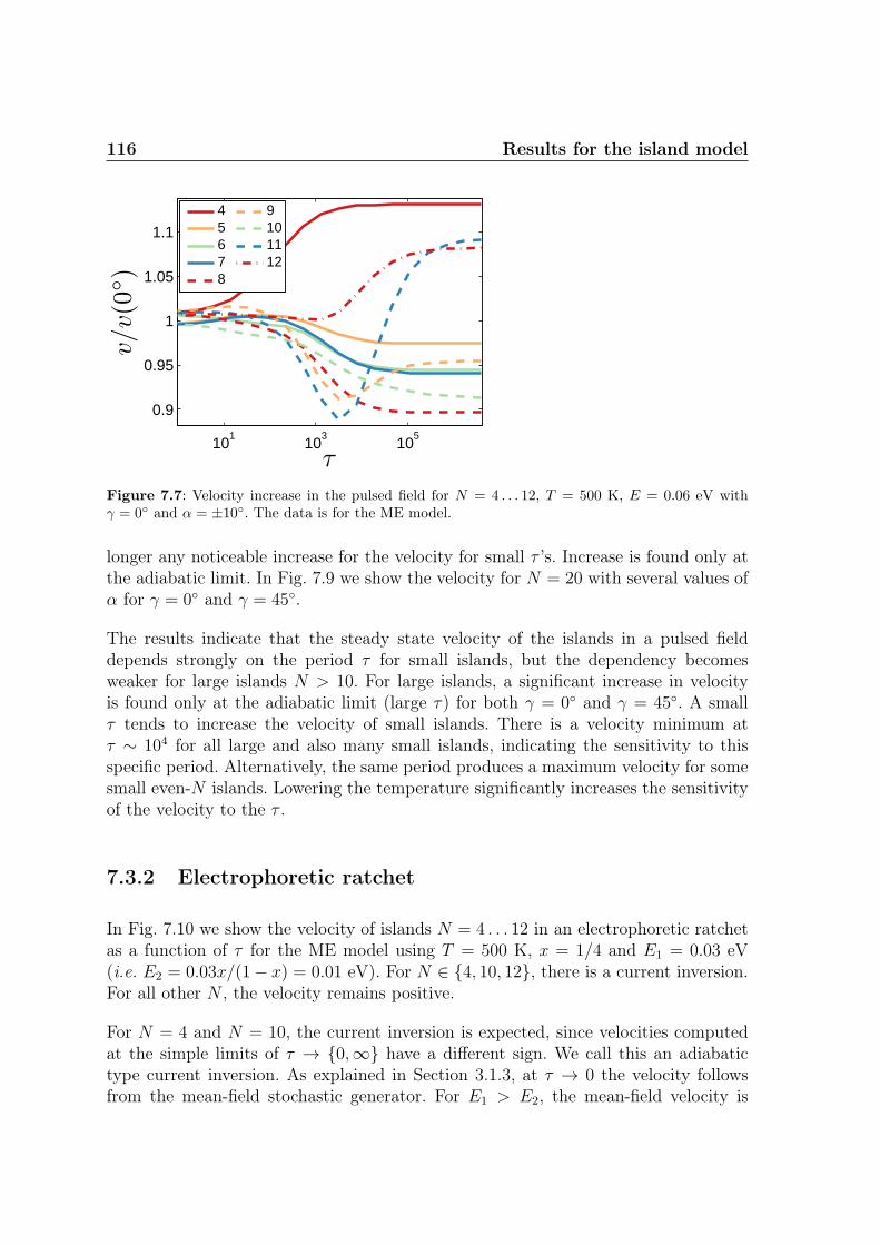
116 Results for the island model
101
103
105
0.9
0.95
1
1.05
1.1
τ
v/v(0
)
45678
9101112
Figure 7.7: Velocity increase in the pulsed field for N = 4 . . . 12, T = 500 K, E = 0.06 eV withγ = 0 and α = ±10. The data is for the ME model.
longer any noticeable increase for the velocity for small τ ’s. Increase is found only atthe adiabatic limit. In Fig. 7.9 we show the velocity for N = 20 with several values ofα for γ = 0 and γ = 45.
The results indicate that the steady state velocity of the islands in a pulsed fielddepends strongly on the period τ for small islands, but the dependency becomesweaker for large islands N > 10. For large islands, a significant increase in velocityis found only at the adiabatic limit (large τ) for both γ = 0 and γ = 45. A smallτ tends to increase the velocity of small islands. There is a velocity minimum atτ ∼ 104 for all large and also many small islands, indicating the sensitivity to thisspecific period. Alternatively, the same period produces a maximum velocity for somesmall even-N islands. Lowering the temperature significantly increases the sensitivityof the velocity to the τ .
7.3.2 Electrophoretic ratchet
In Fig. 7.10 we show the velocity of islands N = 4 . . . 12 in an electrophoretic ratchetas a function of τ for the ME model using T = 500 K, x = 1/4 and E1 = 0.03 eV(i.e. E2 = 0.03x/(1− x) = 0.01 eV). For N ∈ 4, 10, 12, there is a current inversion.For all other N , the velocity remains positive.
For N = 4 and N = 10, the current inversion is expected, since velocities computedat the simple limits of τ → 0,∞ have a different sign. We call this an adiabatictype current inversion. As explained in Section 3.1.3, at τ → 0 the velocity followsfrom the mean-field stochastic generator. For E1 > E2, the mean-field velocity is

7.3 Time-dependent field 117
101
103
105
0.8
1
1.2
1.4
1.6
1.8
v/v(4
5)
45678
9101112
101
103
105
0.5
1
1.5
τ
101
103
105
107
0.8
0.85
0.9
0.95
1
1.05
τ
v/v(4
5)
0.030.040.050.06
0.070.080.090.1
(b)
(c)
(a)
Figure 7.8: Velocity increase in a pulsed field for several small islands with γ = 45 and T = 500 K.(a)-(b) N = 4 . . . 12, T = 500 K, E = 0.06 eV with (a) α = 45 ± 20 and (b) α = 45 ± 50. (c)Distinctive behavior of N = 8 with E = 0.03 . . . 0.1 eV and α = 45± 30.

118 Results for the island model
102
104
106
0.9
0.95
1
1.05
1.1
τv/v
(45
)
1518.922.926.8
30.734.638.6
102
104
106
0.9
0.95
1
1.05
τ
v/v
(0)
1012.915.818.821.724.627.5
(a) (b)
Figure 7.9: Velocity increase in a pulsed field with several pairs of the field angle α (values |α− γ|are shown in the figure) for N = 20 and T = 600 K with field amplitude E = 0.05 eV for (a) γ = 0
and (b) γ = 45. The data is for the MC model.
expected to be positive in the non-linear regime, because of the exponential rates.3
At the adiabatic limit τ → ∞, the velocity approaches vad = xv(E1)− (1− x)v(E2).The sign of vad therefore results from the shape of the velocity curve v(E), which canbe non-monotonous and depends strongly on the island size (see Fig. 7.1). Thereforeboth signs for vad are possible in theory. For the island model, the negative sign forvad is typical for N = 4 and N = 10, but very rare for others. For N = 12, thesimple limits typically yield the same sign and instead the inversion results from atime-dependent field in a non-trivial fashion.
The velocity for N = 12 is shown in more detail in Fig. 7.11 with temperatureT = 500 K and T = 700 K and several field amplitudes. The temperature and thefield amplitude have a very large effect on the velocity in an electrophoretic ratchet.The current inversion easily disappears for increasing the temperature or the fieldamplitude.
The results for the MC model are similar. There are indeed deep minima for τ =104 . . . 106 for large islands which creates a current inversion. This is shown in Fig. 7.12for several islands. For large islands, two local maxima appear at τ = 103 . . . 104. Sincethe current inversion occurs typically only at finite values of τ , it is indeed caused bythe interaction between time-dependent field and atoms. For small islands N < 15,there is a strong odd-even island size dependency which eventually disappears forlarger islands. For an electrophoretic ratchet this odd-even effect becomes importantalready at much smaller fields than in the case of a static field. This is because the
3For example, consider a single free particle affected by the field E1 > 0 on the right and E2 =E1x/(1 − x) on the left with temporal periods τ1 = xτ and τ2 = (1 − x)τ . For the corresponding
mean field rates Γright and Γleft, one hasΓright
Γleft= xeE1+(1−x)e−E2
xe−E1+(1−x)eE2> 1 for 0 < x < 1/2, i.e. the mean
field drift ΓR − ΓL > 0 is always on the right.

7.3 Time-dependent field 119
101
103
105
107
−0.5
0
0.5
1
τ
107v
456
789
101112
Figure 7.10: Velocity in an electrophoretic ratchet with N = 4 . . . 12 and x = 1/4 as a function ofτ with T = 500 K and E1 = 0.03 eV. The data is for the ME model.
102
104
106
0
5
10
15
τ10
210
410
610
8−0.1
0
0.1
0.2
0.3
0.4
τ
108
v
0.010.0190.0270.036
0.0440.0530.0610.07
(a) (b)
Figure 7.11: Velocity in an electrophoretic ratchet with N = 12 and x = 1/4 as a function of τ forseveral field amplitudes E = 0.01 . . . 0.07 eV with (a) T = 500 K and (b) T = 700 K. The data is forthe ME model.

120 Results for the island model
5 10 20 40 90−8
−6
−4
−2
0
N10
7m
in[v
(τ)]
0.020.040.06
103
104
105
106
−4
−3
−2
−1
0
1
2
τ
107v
2050901503005001000
(b)(a)
Figure 7.12: Velocity in the electrophoretic ratchet with T = 600 K and x = 1/4 for the MC model.(a) Velocity for the large islands as a function of τ for E1 = 0.04 eV. (b) Minimum velocities forseveral islands N = 4 . . . 91 for E1 = 0.02 . . . 0.06 eV.
ratcheting mechanism with an alternating field direction tends to force islands intothin rectangular shapes.
We conclude that the τ -dependency in an electrophoretic ratchet is found to be muchstronger than in the case of a pulsed field. With suitable field periods τ around104 . . . 106, a velocity inversion occurs for all large islands (N > 10) and also forsmaller even-N islands. Especially for smaller islands with N < 20, the inversiondepends strongly on the temperature and field strength, disappearing at large tem-peratures. Compared to velocity increase in a pulsed field, inversion phenomena areobserved already with very small field amplitudes near the linear response regime(E ∼ 0.01 eV). An electrophoretic ratchet have been previously studied within thecontext of reptating polymers where a similar type of current inversion was found asa function of polymer size [134].
7.4 Transition sequences
In this Section, we present typical transport mechanisms computed using the cycleoptimization method of Section 5.2.1 for small islands using the ME model. We foundthat the dominating transport cycles for time-dependent fields are usually the same asthose for the static field, especially for the electrophoretic ratchet where two directionsof motion are competing. Also the results for the γ = 0 and γ = 45 are qualitativelysimilar (the ’zig-zag’ configurations appear only for islands much larger than N = 12).

7.4 Transition sequences 121
1 2 3 4
5 6 7 8
9 10 11
(a)
1 2 3 4
5 6 7 8
9 10 11 12
13 14
(b)
Figure 7.13: The dominating transport cycle for (a) N = 11 and (b) N = 12 in large fields in axisdirection.
For time-dependent fields, dominating cycles differ from the static field case only forsmall values of τ , for which the islands have no time to go through a full static-field-type cycles before the potential is changed. Therefore the dominating transport cyclescannot be used to explain the velocity increase by a pulsed field in large τ limit orvelocity inversion for the electrophoretic ratchet with τ = 104 . . . 106. In the following,we set T = 600 K and try various field amplitudes E and report a few optimal cyclesof the type (5.6), with function f being the displacement matrix D. It was found thatthe results are usually the same for both (5.5) and (5.6).
In a static field, typically two kinds of dominating cycles are found corresponding tothe small and large fields. For small fields, E < 0.1 eV, the island remains nearlysquare and for large fields, E > 0.1 eV, the island becomes flatter. In Fig. 7.13 weshow dominating transport cycles for (a) N = 11 and (b) N = 12 in a large axis-directed field. The cycle shown for N = 11 is found for all small odd-N islands in largefields and proceeds by breaking only single nearest-neighbor bonds. This is a similarmechanism as previously proposed being the easiest diffusion pathway for N = 5[183]. For N = 12 and other small even-N islands, the previous type cycle wouldlead to configuration that requires breaking of two nearest-neighbor bonds, whereasthe optimized cycle shown in Fig. 7.13(b) can work with only single bond-breakingtransitions. Unlike one might expect based on the Fig. 7.2, optimal cycles involvingislands with an expected width 1 are not found even for very large fields E ≈ 0.25 eV.This is probably because of the trap configurations that appear for the ME model.
In Fig. 7.14, we show the dominating cycles in the pulsed field case for N = 9 andN = 10 with small τ . In Fig. 7.14(a) the cycle is shown for N = 9 using γ = 0 and

122 Results for the island model
1 2 3 4 5
6 7 8 9 10
11 12 13 14 15
16 17 18 19 20
21 22
(a)(b)
1 2 3 4 5
6 7 8 9 10
11 12 13 14 15
16 17 18 19 20
Figure 7.14: A dominating cycles in pulsed field with small τ . (a) N = 10 with γ = 45 andα = 45 ± 25, gray color indicates α = 20 state. (b) N = 9 with γ = 0 and α = ±20, gray colorindicates α = −20 state.
α = ±20, and in figure Fig. 7.14(b) for N = 10, γ = 45 and α = 45 ± 20. Withthese parameters, the velocity is increased when compared to the static field case (seeSection 7.3.1). The configurations for α = −20 and α = 20 are shown in gray and thechange of potential occurs between the gray and black frames. The cycles are basicallythe same as for the static field case except that the barriers for the transitions arelowered due to the pulsed field. This stochastic-resonance-type mechanism, where thetime-scales of two processes are matched, explains the results seen in Section 7.3.1 forthe increase of the velocity for small τ .
7.5 Discussion
We have studied the dynamics of single-layer metal-on-metal islands under strongstatic and time-dependent forces with a continuous-time Monte Carlo and numeri-cal master equation methods. The aim was to study complex non-linear transportphenomena arising when islands are driven out of equilibrium, far beyond the linearresponse regime. Several non-linear effects were identified, most importantly the in-crease of the velocity by a rotated field and velocity inversions in the electrophoreticratchet. Although the behavior was found to be highly complex, depending stronglyon many parameters such as temperature, field (angle, amplitude and period) andisland size, generic behavior could be identified.
First, we studied static-field transport up to field strengths corresponding single bond-

7.5 Discussion 123
breaking energy barrier (i.e. term EB in Eq. (3.3), 0.260 eV for Cu(001)). For largefields, many differences arise when compared to equilibrium or linear-response condi-tions because typical island configurations are no longer nearly square, but are heavilydeformed by the field. A strong even-odd dependence on the island size was found,which has an influence to even large islands (up to ∼100 atoms). The range of fieldamplitudes E = 0.01 . . . 0.1 eV for Cu was found to be especially interesting from thepoint of view of velocity increase and inversion, since for larger fields these phenom-ena tend to disappear. In this regime, the model is also expected to remain somewhatrealistic, based on the observations of the island geometry changes (no rod configu-rations) and simulations (small island break-up rate). This is also the regime, wherethe results for the MC and ME models coincide. The direction of the field with re-spect to the axis was found to have a large effect on the drift. Introducing a smalldeviation between the measurement and field angles usually leads to an increased ve-locity. Although this is expected in the case of the diagonal measurement direction,it was also found in the direction of axis, which purely results from many-particleinteractions coupling the internal degrees of freedom with the center-of-mass motion.A two-maxima structure for the velocity was found as a function of the field angle. Bycomputing the second-highest eigenvalue of the stochastic generator (the highest onebeing zero), it was found that the leading relaxation time displays a non-monotonousbehavior as a function of the field strength for small islands. The physical meaning ofthis is unclear and further studies are needed.
When a periodic time-dependent variation was added to the field, a complex de-pendence between the velocity and the field period was found. First we studied thepulsed-field case using symmetrically rotated fields around the measuring directionalong the axis and the diagonal. It was found that the velocity was increased at verylarge periods (i.e. slowly varying field), and maxima/minima were found for smallerperiods. The second type of field was an electrophoretic ratchet that creates a time-dependent force with a zero mean force. It was found to produce current inversionsfor all large islands. There are two types of inversion: a genuine time-dependent in-version and an adiabatic inversion for a slowly varying field. Since current inversionsare not possible for a single atom, it is a pure many-particle effect. In theory, thistype of electrophoretic ratcheting would allow separation of islands based on theirsize. In contrast with the velocity increase phenomenon for the pulsed field, currentinversion occurs already in very small fields near linear response regime. One must,however, note that velocities in the electrophoretic ratchet are very small comparedto velocities in non-zero mean force fields.
For both types of time-dependent fields, it was found that for certain large fieldswitching periods (namely for τ = 104 . . . 106 for temperatures T = 400 . . . 700K),the velocity has a minimum for large islands. This time scale corresponds to an atombreaking two nearest neighbor bonds, which is the effective energy barrier processfound in this and all previous studies for this model.

124 Results for the island model
Our results indicate that the typical large island behavior begins already for islandswith just above 10 atoms and the small-size effects become much weaker for largerislands. A similar result was also found in previous studies in equilibrium [183]. Forthis reason, the behavior of the 10 atom island was found to be somewhat special.Most phenomena found in this work can already be produced with islands up to 12atoms. In general, lowering the temperature tends to make velocity increase, currentinversion and τ sensitivity much stronger at the expense of significantly reducing theabsolute velocities. The current inversion in the electrophoretic ratchet may disappearcompletely in large temperatures. This indicates that a large separation in time scalesis a required element for these phenomena (at high temperature limit, all rates becomeequal). Increasing the field amplitude amplifies the velocity increase and inversion upto some point. Very strong fields, however, can have a decreasing effect. Because of thiscomplex dependence on temperature and the field, a data collapse by dimensionlessE/T is not possible far from equilibrium, which is in contrast to the linear responseregime [122].
The ME and MC models were found to be generally in good agreement. Using suitableparameters, both models were able to reproduce most of the key findings of thisChapter - especially in small fields. The largest differences were found for the smallestislands N < 8, for which the aggressive state reduction (i.e. the island must beconnected via nearest-neighbor bonds) of the ME model appears to have the largesteffect. The vacancy diffusion process was not found to have any significant effect forthe ME model. Also, the type of the variation of the field, stochastic or deterministic,was found to have only a minor effect. This is because the time-scale separationof different processes are large, hence the time-scales remain well separated also forrandom field periods.
By applying the ME model, we were able to investigate large portions of the parameter-space with high accuracy, compute effective exponents of the Arrhenius curves, relax-ation times and also identify typical reaction pathways of the islands during transport.The numerically exact ME method shows its power in making the non-linear effectsand their systematics discernible. However, the MC model arguably remains physi-cally more realistic than the ME for the treatment of atoms diffusing around a cornerand for the deterministic field switching scheme.
Since the barrier structure of our semi-empirical model for the processes on fcc(100)surface is quite generic [123], one can expect similar non-linear phenomena to bepresent also in other metal-on-metal systems. As long as distinctive barriers exist, thenon-linear transport properties reported here are not limited to any precise values ofbarriers. Although our model is simple, it displays a rich variety of phenomena. Thisemphasizes the complexity of nonequilibrium many-particle systems and that there isstill much to be done in exploring transport in the presence of time-dependent fields.

7.5 Discussion 125
As discussed in Section 3.4.1, the electromigration force currently achievable in ex-periments is too small to cause strong non-linear effects discussed here. Our simplemodel does not allow a direct comparison with experimental data, but our conclusionsare generic in nature. By introducing more accurate energetics and adding new micro-scopic transition types, it is possible that some phenomena disappear while new onesappear, which we demonstrated by comparing the MC and ME models. It would bealso interesting to study similar properties on other lattice geometries such as close-packed surfaces, with the effect of steps, strain, detachment/attachment processesand other types of driving or interfering forces included. Experimental results for anelectrophoretic ratchet mechanism in the absence of periodic potentials would be ofinterest also for other types of two and three-dimensional many-particle systems. Onemay assume that current inversions are indeed common. So far these experiments havebeen limited to study DNA separation techniques [72, 171, 172].

8 Summary
In this work, we have studied nonequilibrium properties of many-particle systems bynumerically solving master equations using linear algebra (’direct’) and by MonteCarlo (’indirect’) methods. The focus of this work has been in solving the transportproperties with a direct method. We have thoroughly discussed relevant practical as-pects of the theory and the numerics of master equations and their applicability in thestudies of complex many-particle models. We have tested a suitable set of linear alge-braic and optimization methods related to the direct method. Both direct and indirectmethods were applied to study transport of polymers and metal-on-metal islands innon-homogeneous time-dependent potentials. Although the equilibrium properties ofthese models are well known, predicting transport properties far from equilibrium isvery difficult, because the velocity and diffusion coefficient no longer have a linearrelationship. Currently, the only way to gain access to such nonequilibrium propertiesis by simulation or by solving corresponding master equations numerically.
Although the repton and island migration models are different, they share many com-mon properties. Because of the similar structure with roughly same number of edgesper nodes in the transition graphs, both models exhibit similar numerical behavior inlinear algebraic and integration computations. Both models also exhibit explicit non-monotonous response to the potential strength. For models with more than one spatialdimension, the directions of the potential and measuring are of a special interest be-cause of inherent spatial anisotropy. As seen for the island model, a properly chosendirection can increase the velocity. For time-dependent potentials, velocity minima andmaxima typically appear as a function of the temporal period of the potential. Thisis caused by correlations between the time-scales of the center-of-mass displacementand internal configurations of the many-particle system. The most striking feature isthe current reversal phenomenon that was found in both repton and island models.Although this phenomenon is quite typical when the direction of the forces caused bythe potential are changing (e.g. flashing ratchet potential and electrophoretic field), itsoccurrence and details depend strongly on the details of the model. Detailed discussionof results can be found in the discussion sections of Chapters 6 and 7.
Hopefully the results and methods presented in this work also support the effortsto better understand cooperative transport occurring in biological systems and todevelop complex artificial molecular motors. Especially having externally adjustableparameters to control molecular motors, such as time-dependent potentials studied inthis work, are an important aspect in designing artificial molecular motors [93, 19].
126

top page line 127
Due to the advances in computer technology and numerical methods, direct solutionof the master equation has become a practical method only within the last decade orso. As demonstrated in this work, an ordinary desktop computer can handle systemslarge enough for large-system characteristics to appear. The master equation methodhas several advantages. The most important is its numerical accuracy, which canbe typically pushed all the way to the extent of floating point arithmetics for non-stiff master equations. Even for stiff systems, the accuracy is usually much betterthan in Monte Carlo simulations. The second advantage is that the computationis fast, which allows more extensive exploration of the parameter space. Unlike theMonte Carlo method, the master equation method is typically robust against thechoice of the initial state, and the arrival to the steady state is straightforward toverify. Also less manual work is required to compute, verify and analyze the resultsas compared to what is typically needed in the Monte Carlo method. Good accuracy,rapid computations and full knowledge of the available configuration space allow usingefficient optimization methods to find optimal parameters and transition cycles.
The most severe limitation of the master equation method is the size limitation. Inthis work, the practical upper limit for stochastic many-particle systems with sparsetransition graphs (e.g. repton, island and TASEP models) was found to be around106 states. This limit is often easily met, since the number of states typically growsexponentially with the number of particles. The upper limit is set by the scaling ofthe computing time and memory consumption as a function of the number of equa-tions. Iterative algorithms that are applied to solve eigenstates, linear problems, andoptimize cycles and parameters, are beyond linear. Therefore simply increasing thecomputing power and time cannot overcome the size limitations. To study larger sys-tems, reduction methods (e.g. DMRG) must be applied, which however makes themethod less robust and numerically unpredictable because of additional approxima-tions. Compared to Monte Carlo method, the master equation method is not wellsuited for studying non-Markovian systems. Also setting up the master equation setsand related operators takes some effort, whereas in Monte Carlo simulation, knowingthe full configuration space is not required.
There are several ways to extend this work. Detailed discussion for extending the stud-ies of repton and island models can be found in the discussion sections of Chapters 6and 7. The presented framework including computational methods and model analy-sis are, however, readily applicable to other models as well. For the master equationmethod, large separation of timescales makes the equation set stiff, which causes severenumerical instabilities and inaccuracies. Current techniques to overcome this problemare typically based on the assumption of quasi-steady states [44, 135, 146]. However,these techniques cannot be directly applied to study transport in many-particle sys-tems, because stochastic generators are often too complicated and one must also keeptrack of displacements. Instead, a desired way would be to apply idea of Ref. [163],where both stochastic generator and related operators (e.g. a displacement matrix)

128 Summary
were reduced to smaller ones. Turning this procedure into a general and numericallyefficient algorithm is, however, technically challenging. The cycle optimization resultsin this work suggests that dominating cycles remain relatively short even for large sys-tems. Since the total number of short cycles is quite small, optimization with generalweight functions might be possible, at least approximatively. Finally, in order to makea numerical master equation method a standard numerical tool to study transport incomplex nonequilibrium systems, a comprehensive testing of available numerical linearalgebraic, optimization and reduction methods and different types of many-particlemodels would be in order.

A Time-dependent DMRG
In this Appendix, we describe the time-dependent DMRG method. Steps concerningthe construction of the operators are model-specific and are discussed in detail inSection 4.1.1 for the repton model. Here we only go through the basic working princi-ples behind the method, technical details can be found in Ref. [166]. Time-dependentDMRG is based on the normal DMRG, which is often called the ground-state DMRGmethod, so we begin with that.
Consider a one-dimensional many-particle system (such as a Heisenberg or a reptonchain) in a state |Ψ〉, which is either a wavefunction or a probability distribution forthe ground state or the steady state. This is called a target state and more than onetarget state can be used. Instead of presenting this state in the basis of the full systemof all sites, we can alternatively express it as an entangled state of two (or more) sub-systems such that |Ψ〉 =∑N1
i=1
∑N2
j=1 ci,j|i〉 ⊗ |j〉, where |i〉 and |j〉 are basis vectors ofseparate subsystems and ci,j are coefficients. For one-dimensional systems the naturalchoice for subsystems is to use left (basis |i〉) and right (basis |j〉) parts. Theorem,known as Schmidt decomposition, states that there exists orthonormal basis |i1〉 and|i2〉 such that |Ψ〉 = ∑M=min[N1,N2]
i=1 αi|i1〉 ⊗ |i2〉 with∑
i α2i = 1. Such decomposition
can be found by creating and diagonalizing reduced density operators ρ1 and ρ2 withelements [ρ1]i,i′ =
∑j c
†i,jci′,j and similarly for ρ2. By the construction ρ1 and ρ2
have the same spectrum.1 This decomposition is at the center of the DMRG method.Coefficients αi include information about the correlations between subsystems. If thereis no correlation, only one of the coefficients is non-zero [127].
Now suppose that we want to use only n < M basis vectors for the first (left) subsys-tem, i.e. we want to find a truncated state |Ψ〉 ≈ |Ψ〉. By using basic linear algebra,one can show that such truncation minimizing the norm ||Ψ〉 − |Ψ〉|2 is achieved bychoosing the states with largest weights αi. From this partial set of most importanteigenstates, one can create a truncated change-of-basis operator, which can be used totruncate states and operators accordingly. Based on this theoretical framework, during1992-93, White proposed DMRG method to study one-dimensional quantum systems[195]. The proposed algorithms are commonly known as infinite-size and finite-sizealgorithms. The infinite-size algorithm is used to construct reduced operators for largesystems by starting with a small system, which can still be diagonalized exactly. Then
1In practical computations, typically one only needs to find a truncated basis for one of theblocks (the ’system’). Given a target state(s) and block dimension, this can be done without creatingdecompositions and more than one density matrix.
129

130 Time-dependent DMRG
one increases the system size by adding new sites and using the truncation procedurebased on density matrices and Schmidt decomposition. The finite-size algorithm issimilar, but instead of increasing the system size, it is used to improve the state andoperators created with the infinite-size algorithm.
We now present the basic steps of the infinite-size algorithm, which already includesthe central parts of the DMRG method.
1. By using the left and right subsystems, form a superblock Hamiltonian H con-taining L sites and having dimension N1 ×N2.
2. Compute the ground/steady state |Ψ〉 =∑N1
i=1
∑N2
j=1 ci,j|i〉 ⊗ |j〉 for H.
3. Form the reduced density matrix ρ1 =∑N1
i,i′=1
∑N2
j,j′=1 ci,jc∗i′,j′ |i〉〈i′| for the left
part and similarly ρ2 for the right one.
4. Diagonalize ρ’s to obtain n1 < N1 and n2 < N2 eigenvectors with the largesteigenvalues separately for the left and right part. Using these vectors, create areduced basis transformation operators O1 and O2.
5. Transform Hamiltonians and all associated operators for both subsystems intotheir reduced eigenbasis using O operators.
6. Add new sites into the newly reduced subsystems. Now the total number of sitesin the subsystems is N + 2. Goto step 1. Now L → L + 2, N1 → n1 ×M1 andN2 → M2 × n2, where M1 and M2 are the dimensions of new sites (typicallyM1 =M2).
To increase the accuracy and stability, infinite-size algorithm should be always ac-companied by the finite-size version. The finite-size algorithm is a modification ofthe above scheme. Instead of increasing the system size, one keeps the system size Lfixed all the time and performs ’sweeping’. Sweeping is done by adding new sites intoone block while reducing them from the other. Operators for the shrunk blocks areretrieved from the memory in which they were stored during previous steps (eitherduring infinite-size algorithm or previous sweeps). After couple of such sweeps, whereboth blocks have been fully shrunk and grown, more accurate operators and targetstate(s) are obtained. See Fig. A.1 for an illustration of the both infinite-size algorithmand sweeping.
Dividing the system into smaller parts and then using the information of all partsto reduce the subsystems is the key idea of the DMRG method. The amount ofentanglement between subsystems regulate the success of the truncation [7]. Basistruncation is kept under a given truncation tolerance, which is typically small (e.g. ∼10−10). This is the single most important parameter in the method. Block sizes are

131
increased step-by-step and it is required that the operators can be build recursively.The size of the reduced basis must remain small, typically less than a hundred or so.Due to its working principle, DMRG can be efficiently applied only to one-dimensionalsystems with short interaction lengths. There has been attempts to extend DMRGtechnique to include two-dimensional systems and more complicated many-particleinteractions, but with poor results. The best performance is received for open system,although periodic systems can be also handled with less precision.
Instead of targeting the ground or steady states, one can also target time-dependentstates. This is the case with the time-dependent DMRG method which uses Runge-Kutta approach [58]. After computing the target state |Ψ(t)〉 at t = 0 using time-step∆t and the infinite and finite-size algorithms, one can compute
|k1〉 = ∆tH(t)|Ψ(t)〉|k2〉 = ∆tH(t+∆t/2) [|Ψ(t)〉+ 1/2|k1〉]|k3〉 = ∆tH(t+∆t/2) [|Ψ(t)〉+ 1/2|k2〉]|k4〉 = ∆tH(t+∆t) [|Ψ(t)〉+ |k3〉] .
Using these, approximations for the intermediate states are
|Ψ(t+∆t/3)〉 ≈ |Ψ(t)〉+ 1
162[31|k1〉+ 14|k2〉+ 14|k3〉 − 5|k4〉]
|Ψ(t+ 2∆t/3)〉 ≈ |Ψ(t)〉+ 1
81[16|k1〉+ 20|k2〉+ 20|k3〉 − 2|k4〉]
|Ψ(t+∆t)〉 ≈ 1
6[|k1〉+ 2|k2〉+ 2|k3〉+ |k4〉] ,
which are used as the target states. After sweeping, all operators are well adapted tothese states and one can advance t+∆t in time and repeat the process.
During the past 20 years a large number of modifications and improvements of theseoriginal algorithms have been proposed, involving different block arrangements, finite-temperature extension, state estimation and better targeting, time-development andtechnical improvements. More recently, focus has shifted towards matrix product stateformalism, instead of working with matrices and vectors as presented here. This haslead to new extension of the DMRG method and better theoretical understandinghow it works [166].

132 Time-dependent DMRG
= block
= site
3.
2.
1.
. . .
. . .
. . .
Figure A.1: Illustrations of the DMRG procedures. On the left, one iteration of the infinite-systemDMRG algorithm is shown: (1) Free sites are added in left and right blocks, (2) the super-block isformed and a target state (e.g. the steady state) is solved, (3) both blocks are renormalized. On theright, one complete ’sweeping’ for the finite-size algorithm and time-dependent DMRG is shown.

B Derivation of equations (4.2) and(4.3)
In this Section we derive equations (4.2) and (4.3), which are valid for any finitemaster equation system. The derivation follows the seminal work by Derrida [46] andlater works closely related to it, such as [64, 26, 101, 178]. For a general system, weare only able to derive the equations which are to be solved using numerical methods.See also Ref. [188] where similar derivation is done for the discretized Fokker-Planckequation.
Let us consider a finite discrete stochastic system with states y ∈ 1, 2, . . . , N and letus define a real-valued counting process x, such as the displacement of the center-of-mass, given by an antisymmetric matrix D, i.e. moving from state i to j increases (ordecreases) the counter by Dj,i and with Di,i = 0 and no branching. Then for an ergodicsystem, one can start from any state and construct the relative spatial positions ofall N states using D, this defines values xy ∈ R for the counter. Let the primitiveperiod of the counter be L > 0 and define xly := xy + Ll with l ∈ Z. This means,that in the configuration graph of the model, there exists one or more simple cyclesC such that
∑〈i,j〉∈C Di,j = L. For the center-of-mass transport in particle models,
one may conclude that there cannot be simple cycles with a different L, because theperiod is bind to the displacement of the center-of-mass, which results from a precisenumber if single particle moves (e.g. reptons or atoms)1. However, this is merely atechnical requirement to simplify the derivation. As we will see, expressions for v(t)and Deff(t) only depend on H and D. Finally, note that one can have xl
′
y′ = xly forsome l′ 6= l and/or y′ 6= y. This is typically the case when the configuration graph hasa complicated structure.
Let the joint probability for a state y in a period l be given by ply with its time-evolutiongiven by the master equation
dply(t)
dt=∑
y′
[Hy,y′p
l+f(y,y′)y′ (t)−Hy′,yp
ly(t)],
where Hy,y = 0 and the anti-symmetric function f takes values −1, 0, 1, dependingon whether the state y′ actually belongs to the previous (l−1), the same (l) or the next
1Because |xkl − xy
l | is fixed for all l, the assumption of two or more different periods immediatelyleads to a contradiction
133

134 Derivation of equations (4.2) and (4.3)
(l+1) period. This ’bookkeeping’ function depends on how one chooses xy. However,as we will see, it has no effect on the final results because it will disappear in thesummation over all periods l. The nth moment of the counter is
〈xn(t)〉 =∞∑
l=−∞
∑
y
(xly)nply(t).
Definitions for the velocity and the effective diffusion coefficient are given in Sec-tion 3.2.1. After these preliminaries, let us begin the derivation by defining followingauxiliary functions
qy(t) =∞∑
l=−∞
ply(t)
sy(t) =∞∑
l=−∞
xlyply(t)− 〈x(t)〉qy(t),
where x(t) is the value of the counter at time t. One can see that conditions∑
y qy = 1and
∑y sy = 0 hold. From now on, we drop the explicit t-dependency to simplify the
notation. Taking time derivative and using master equations, we have
qy =∞∑
l=−∞
∑
y′
[Hy,y′p
l+f(y,y′)y′ −Hy′,yp
ly
]=∑
y′
[Hy,y′qy′ −Hy′,yqy]
sy =∞∑
l=−∞
xly∑
y′
[Hy,y′p
l+f(y,y′)y′ −Hy′,yp
ly
]− d〈x〉
dtqy − 〈x〉qy.
For the value of the counter, we can write xly = xl+f(y,y′)y′ +Dy,y′ for states y′ reachable
from y. Now we can re-arrange terms
sy =∞∑
l=−∞
∑
y′
[Hy,y′
(xl+f(y,y′)y′ +Dy,y′
)pl+f(y,y′)y′ −Hy′,yx
lyp
ly
]− 〈x〉
∑
y′
[Hy,y′qy′ −Hy′,yqy]
− d〈x〉dt
qy
=∑
y′
Hy,y′
[∞∑
l=−∞
xl+f(y,y′)y′ p
l+f(y,y′)y′ − 〈x〉qy′
]−∑
y′
Hy′,y
[∞∑
l=−∞
xlyply − 〈x〉qy
]
+∑
y′
Hy,y′Dy,y′
∞∑
l=−∞
pl+f(y,y′)y′ − d〈x〉
dtqy
=∑
y′
[Hy,y′sy′ −Hy′,ysy +Hy,y′Dy,y′qy′ ]−d〈x〉dt
qy.

135
Time-derivatives of the first two moments can be now computed.
v(t) =d〈x(t)〉dt
=∞∑
l=−∞
∑
y′
xly′∑
y
[Hy′,yp
l+f(y′,y)y −Hy,y′p
ly′
]
=∑
y
∑
y′
∞∑
l=−∞
[xl+f(y′,y)y Hy′,yp
l+f(y′,y)y +Dy′,yHy′,yp
ly − xly′Hy,y′p
ly′
]
=∑
y
∑
y′
Dy′,yHy′,y
∞∑
l=−∞
ply
=∑
y′
∑
y
Dy′,yHy′,yqy.
By using identity(xly′)2
=(xl+f(y′,y)y
)2+ 2Dy′,yx
l+f(y′,y)y +D2
y′,y, we get
d〈x(t)2〉dt
=∞∑
l=−∞
∑
y′
(xly′)2∑
y
[Hy′,yp
l+f(y′,y)y −Hy,y′p
ly′
]
=∞∑
l=−∞
∑
y
∑
y′
[(xl+f(y′,y)y
)2+ 2Dy′,yx
l+f(y′,y)y +D2
y′,y
]Hy′,yp
l+f(y′,y)y
−(xly′)2Hy,y′p
ly′
=∞∑
l=−∞
∑
y
∑
y′
[2Dy′,yx
l+f(y′,y)y +D2
y′,y
]Hy′,yp
l+f(y′,y)y
=2∑
y
∑
y′
Dy′,yHy′,y
∞∑
l=−∞
xlyply +
∑
y
∑
y′
D2y′,yHy′,yqy.
Inserting these into the definition of Deff(t), with d = 1, we get
Deff(t) =1
2
d〈x(t)2〉dt
− 〈x(t)〉d〈x(t)〉dt
=∑
y
∑
y′
Dy′,yHy′,y
∞∑
l=−∞
xlyply +
1
2
∑
y
∑
y′
D2y′,yHy′,yqy − 〈x〉
∑
y′
∑
y
Dy′,yHy′,yqy
=∑
y
∑
y′
Dy′,yHy′,y
[∞∑
l=−∞
xlyply − 〈x〉qy
]+
1
2
∑
y
∑
y′
D2y′,yHy′,yqy
=∑
y
∑
y′
Dy′,yHy′,ysy +1
2
∑
y
∑
y′
D2y′,yHy′,yqy.
In the case of time-independent H, taking the limit t→ ∞ gives the long-time velocityand diffusion coefficient for the center-of-mass transport. For time-dependent systems,integration over time is required.

References
[1] R. K. Ahuja, T. L. Magnanti, and J. B. Orlin: Network Flows: Theory, Algo-rithms, and Applications, Prentice Hall, New Jersey (1993).
[2] B.-Q. Ai and L.-G. Liu: Current in a three-dimensional periodic tube with un-biased forces, Phys. Rev. E 74, 051114 (2006); D. Reguera, G. Schmid, P. S.Burada, J. M. Rubi, P. Reimann, and P. Hänggi: Entropic Transport: Kinetics,Scaling, and Control Mechanisms, Phys. Rev. Lett. 96, 130603 (2006); P. S.Burada, G. Schmid, Y. Li, P. Hänggi: Controlling diffusive transport in confinedgeometries, Acta Physica Polonica B 41, 935 (2010);
[3] B.-Q. Ai , X.-J. Wang, G.-T. Liu, H.-Z. Xie, D.-H. Wen, W. Chen, and L.-G.Liu: Current reversals in an inhomogeneous system with asymmetric unbiasedfluctuations, Eur. Phys. J. B 37, 523 (2004).
[4] R. Ait-Haddou and W. Herzog: Brownian Ratchet Models of Molecular Motors,Cell Biochemistry and Biophysics 38, 191 (2003).
[5] T. Ala-Nissilä, R. Ferrando, and S. C. Ying: Collective and single particle dif-fusion on surfaces, Advances in Physics 51, 949 (2002).
[6] D. Aldous and J. A. Fill: Reversible Markov chains and random walks on graphs,(unpublished), http://www.stat.berkeley.edu/~aldous/RWG/book.html.
[7] L. Amico, R. Fazio, A. Osterloh, V. Vedra: Entanglement in many-body systems,Rev. Mod. Phys. 80, 517 (2008).
[8] D. Andrieux and P. Gaspard: Fluctuation Theorem for Currents and Schnaken-berg Network Theory, J. Stat. Phys. 127, 107 (2007); D. Andrieux and P.Gaspard: Network and thermodynamic conditions for a single macroscopic cur-rent fluctuation theorem, C. R. Physique 8, 579 (2007); J. L. Lebowitz and H.Spohn: A Gallavotti-Cohen-Type Symmetry in the Large Deviation Functionalfor Stochastic Dynamics, Journal of Statistical Physics 95, 333 (1999); D. An-drieux and P. Gaspard: Fluctuation theorem for transport in mesoscopic systems,J. Stat. Mech. 1, P01011 (2006).
[9] U. M. Ascher, R. M. M. Mattheij, and R. D. Russell: Numerical Solution ofBoundary Value Problems for Ordinary Differential Equations, SIAM, Philadel-phia (1995).
136

References 137
[10] R. Ashton, C. Padalay and R. S. Kanez: Microfluidic separation of DNA, Cur-rent Opinion in Biotechnology 14, 497 (2003).
[11] R. D. Astumian: Thermodynamics and Kinetics of Molecular Motors, Biophys-ical Journal 98, 2401 (2010); R. D. Astumian: Design Principles for BrownianMolecular Machines: How to Swim in Molasses and Walk in a Hurricane, Phys.Chem. Chem. Phys. 9, 5067 (2007).
[12] R. D. Astumian and M. Bier: Fluctuation driven ratchets: molecular motors,Phys. Rev. Lett. 72, 1766 (1994).
[13] J. S. Bader, R. W. Hammond, S. A. Henck, M. W. Deem, G. A. McDermott, J.M. Bustillo, J. W. Simpson, G. T. Mulhern, and J. M. Rothberg: DNA transportby a micromachined Brownian ratchet device, Proc. Natl. Acad. Sci. USA 96,13165 (1999); R. W. Hammond, J. S. Bader, S. A. Henck, M. W. Deem, G.A. McDermott, J. M. Bustillo, and J. M. Rothberg: Differential transport ofDNA by a rectified Brownian motion device, Electrophoresis 21, 74 (2000); J. S.Bader, M. W. Deem, R. W. Hammond, S. A. Henck, J. W. Simpson, and J. M.Rothberg: A Brownian-ratchet DNA pump with applications to single-nucleotidepolymorphism genotyping, Appl. Phys. A: Mater. Sci. Process. 75, 275 (2002).
[14] M. Badoual, F. Julicher, and J. Prost: Bidirectional cooperative motion of molec-ular motors, Proc. Natl. Acad. Sci. USA 99, 6696 (2002).
[15] V. Balakrishnan: Schaum’s Outline of Graph Theory, McGrawn-Hill, New York(1997); J. Bang-Jensen and G. Gutin: Digraphs: Theory, Algorithms and Appli-cations, Springer-Verlag, London (2009).
[16] A. Barrat, M. Barthelemy, and A. Vespignani: Dynamical processes on complexnetworks, Cambridge University Press, Cambridge (2008).
[17] R. Barrett, M. Berry, T. F. Chan, J. Demmel, J. Donato, J. Dongarra, V.Eijkhout, R. Pozo, C. Romine, and H. Van der Vorst: Templates for the Solutionof Linear Systems: Building Blocks for Iterative Methods, SIAM, Philadelphia(1994).
[18] F. Berger, T. Schmiedl, and U. Seifert: Optimal potentials for temperature ratch-ets, Phys. Rev. E 79, 031118 (2009).
[19] V. Bermudez, N. Capron, T. Gase, F. G. Gatti, F. Kajzar, D. A. Leigh, F.Zerbetto, and S. Zhang: Influencing intramolecular motion with an alternatingelectric field, Nature 406, 605 (2000); A. Credi: Artificial Molecular MotorsPowered by Light, Aust. J. Chem. 59, 157 (2006).
[20] L. Bitar, P. A. Serena, P. Garcia-Mochales, N. Garcia, and Vu Thien Binh:Mechanism for diffusion of nanostructures and mesoscopic objects on surfaces,Surf. Sci. 339, 221 (1995).

138 References
[21] B. Bortz, M. H. Kalos, and J. L. Lebowitz: A new algorithm for Monte Carlosimulation of Ising spin systems, J. Comput. Phys. 17, 10 (1975).
[22] M. van den Broek, R. Eichhorn, and C. Van den Broeck: Intrinsic ratchets,Europhys. Lett. 86, 30002 (2009).
[23] M. O. Caceres and A. M. Lobos: Theory of eigenvalues for periodic non-stationary Markov processes: the Kolmogorov operator and its applications, J.Phys. A: Math. Gen. 39, 1547 (2006).
[24] A. M. Cadilhe, C. R. Stoldt, C. J. Jenks, P. A. Thiel, and J. W. Evans: Evolutionof far-from-equilibrium nanostructures on Ag(100) surfaces: Protrusions andindentations at extended step edges, Phys. Rev. B 61, 4910 (2000); S. Pal andK. A. Fichthorn: Size dependence of the diffusion coefficient for large adsorbedclusters, Phys. Rev. B 60, 7804 (1999); H. Mehl, O. Biham, I. Furman, and M.Karimi: Models for adatom diffusion on fcc (001) metal surfaces, Phys. Rev. B60, 2106 (1999); X. Wang, F. Xie, Q. Shi, and T. Zhao: Effect of atomic diagonalmotion on cluster diffusion coefficient and its scaling behavior, Surf. Sci. 561,25 (2004);
[25] E. Carlon, A. Drzewinski, and J. M. J. van Leeuwen: Reptation in theRubinstein-Duke model: The influence of end-reptons dynamics, J. Chem. Phys.117, 2425 (2002).
[26] J. Casado-Pascual: Flux reversal in a simple random-walk model on a fluctuatingsymmetric lattice, Phys. Rev. E 74, 021112 (2006).
[27] D. Chandler: Introduction to modern statistical mechanics, Oxford UniversityPress, New York (1987).
[28] A. Chatterjee and D. G. Vlachos: An overview of spatial microscopic and ac-celerated kinetic Monte Carlo methods, J. Computer-Aided Mater. Des. 14, 253(2007); J. L. Blue, I. Beichl, and F. Sullivan: Faster Monte Carlo simulations,Phys. Rev. E 51, R867 (1995).
[29] V. Y. Chernyak and N. A. Sinitsyn: Pumping Restriction Theorem for StochasticNetworks, Phys. Rev. Lett. 101, 160601 (2008); N. A. Sinitsyn: The stochasticpump effect and geometric phases in dissipative and stochastic systems, J. Phys.A: Math. Theor. 42, 193001 (2009); S. Rahav, J. Horowitz, and C. Jarzynski:Directed Flow in Nonadiabatic Stochastic Pumps, Phys. Rev. Lett. 101, 140602(2008).
[30] J.-Y. Chen, D. R. Kincaid, and D. M. Young: Generalizations and modificationsof the GMRES iterative method, Numerical Algorithms 21, 119 (1999).
[31] H. Chen, Q. Wang, and Z. Zheng: Deterministic directed transport of inertialparticles in a flashing ratchet potential, Phys. Rev. E 71, 031102 (2005).

References 139
[32] Y. D. Chen, B. Yan, and R. Miura: Asymmetry and direction reversal influctuation-induced biased Brownian motion, Phys. Rev. E 60, 3771 (1999).
[33] T. Chou, K. Mallick, and R. K. P. Zia: Non-equilibrium statistical mechanics:from a paradigmatic model to biological transport, Rep. Prog. Phys. 74, 116601(2011).
[34] D. Chowdhury, A. Schadschneider, and K. Nishinari: Physics of Transport andTraffic Phenomena in Biology: from molecular motors and cells to organisms,Phys. of Life Reviews 2, 318 (2005).
[35] B. E. Clancy, W. M. Behnke-Parks, J. O. L. Andreasson, S. S. Rosenfeld, andS. M. Block: A universal pathway for kinesin stepping, Nature structural andmolecular biology 18, 1020 (2011); R. Lipowsky, S. Liepelt, and A. Valleriani:Energy Conversion by Molecular Motors Coupled to Nucleotide Hydrolysis, J.Stat. Phys. 135, 951 (2009).
[36] N. Combe and H. Larralde: Low-temperature shape relaxation of two-dimensional islands by edge diffusion, Phys. Rev. B 62, 16074 (2000); P. Jensen,N. Combe, H. Larralde, J. L. Barrat, C. Misbah, and A. Pimpinelli: Kinetics ofshape equilibration for two dimensional islands, Eur. Phys. J. B 11, 497 (1999);Da-Jiang Liu and J. W. Evans: Sintering of two-dimensional nanoclusters inmetal.100. homoepitaxial systems: Deviations from predictions of Mullins con-tinuum theory, Phys. Rev. B 66, 165407 (2002).
[37] A. R. Conn, K. Scheinberg, and L. N. Vicente: Introduction to derivative-freeoptimization, SIAM, Philadelphia (2009).
[38] E. M. Craig, M. J. Zuckermann, and H. Linke: Mechanical coupling in flashingratchets, Phys. Rev. E 73, 051106 (2006).
[39] W. J. Culver: On the Existence and Uniqueness of the Real Logarithm of aMatrix, Proceedings of the American Mathematical Society 17, 1146 (1966).
[40] A. Dasdan: Experimental Analysis of the Fastest Optimum Cycle Ratio andMean Algorithms, ACM Transactions on Design Automation of Electronic Sys-tems 9, 385 (2004).
[41] A. Dasdan and R. K. Gupta: Faster maximum and minimum mean cycle algo-rithms for system-performance analysis, IEEE transactions on computer-aideddesign of integrated circuits and systems 17, 889 (1998);
[42] A. Dasdan, S. S. Irani, and R. K. Gupta: Efficient algorithms for optimumcycle mean and optimum cost to time ratio problems, Proceedings of the 36th
ACM/IEEE conference on Design automation, 37 (1999).

140 References
[43] T. A. Davis: Direct Methods for Sparse Linear Systems, SIAM, Philadelphia(2006).
[44] T. Dayar and W. J. Steward: Comparison of partitioning techniques for two-level iterative solvers on large, sparse Markov chains, SIAM Journal on ScientificComputing 21, 1691 (2000).
[45] I. Derenyi, M. Bier, and R. D. Astumian: Generalized Efficiency and its Appli-cation to Microscopic Engines, Phys Rev. Lett. 83, 903 (1999).
[46] B. Derrida: Velocity and diffusion constant of a periodic one-dimensional hop-ping model, J. Stat. Phys. 31, 433 (1983).
[47] B. Derrida: Non-equilibrium steady states: fluctuations and large deviations ofthe density and of the current, J. Stat. Mech. 07, P07023 (2007).
[48] R. Dickman: Numerical analysis of the master equation, Phys. Rev. E 65, 047701(2002).
[49] L. Dinis: Optimal sequence for Parrondo games, Phys. Rev. E 77, 021124 (2008).
[50] J. R. Dormand and P. J. Prince: A family of embedded Runge-Kutta formulae,J. Comp. Appl. Math. 6, 19 (1980).
[51] S. Dorosz and M. Pleimling: Characterizing steady-state and transient propertiesof reaction-diffusion systems, Phys. Rev. E 80, 061114 (2009); D. ben-Avraham,S. Dorosz, and M. Pleimling: Realm of validity of the Crooks relation, Phys. Rev.E 83, 041129 (2011).
[52] A. Drzewinski and J. M. J. van Leeuwen: Field induced orientation of reptatingpolymers, J. Stat. Mech. 2, P02004 (2005).
[53] A. Drzewinski and J. M. J. van Leeuwen: Crossover from reptation to Rousedynamics in a one-dimensional model, Phys. Rev. E 73, 061802 (2006); A.Drzewinski and J. M. J. van Leeuwen: Crossover from reptation to Rouse dy-namics in the extended Rubinstein-Duke model, Phys. Rev. E 77, 031802 (2008).
[54] M. T. Downton, M. J. Zuckermann, E. M. Craig, M. Plischke, and H. Linke:Single-polymer Brownian motor: A simulation study, Phys. Rev. E 73, 011909(2006).
[55] T. A. J. Duke: Tube model of field-inversion electrophoresis, Phys. Rev. Lett.62, 2877 (1989).
[56] A. Efremov and Z. Wang: Universal optimal working cycles of molecular motors,Phys. Chem. Chem. Phys. 13, 6223 (2011).

References 141
[57] M. Esposito and K. Lindenberg: Continuous-time random walk for open systems:Fluctuation theorems and counting statistics, Phys. Rev. E 77, 051119 (2008).
[58] A. Feiguin and S. R. White: Time-step targeting methods for real-time dynamicsusing the density matrix renormalization group, Phys. Rev. B 72, 020404 (2005).
[59] M. Feito and F. J. Cao: Optimal operation of feedback flashing ratchets, J. Stat.Mech. 1, P01031 (2009).
[60] A. J. Fendrik, L. Romanelli, and R. P. J. Perazzo: Collective modes in a coupledratchet model, Physica A: Statistical Mechanics and its Applications 368, 7(2006).
[61] H. Feng, B. Han, and J. Wang: Dominant Kinetic Paths of Complex systems:Gene Networks, J. Phys. Chem. Lett. 1, 1836 (2010).
[62] R. P. Feynman, R. B. Leighton, and M. Sands: The Feynman Lectures onPhysics, Pearson/Addison-Wesley, San Francisco (2006).
[63] T. J. Frankcombe and S. C. Smith: Numerical solution methods for large, diffi-cult kinetic master equations, Theor. Chem. Acc. 124, 303 (2009).
[64] J. A. Freund and L. Schimansky-Geier: Diffusion in discrete ratchets, Phys. Rev.E 60, 1304 (1999).
[65] F. R. Gantmacher: The theory of matrices, AMS Chelsea Publishing, Providence(2000).
[66] C. W. Gardiner: Handbook of Stochastic Methods: for Physics, Chemistry andthe Natural Sciences, Springer-Verlag, Berlin (2004); N. G. Van Kampen:Stochastic processes in physics and chemistry, Elsevier, Amsterdam (2007).
[67] P. G. de Gennes: Scaling Concepts in Polymer Physics, Cornell University Press,Ithaca (1979).
[68] S. von Gehlen, M. Evstigneev, and P. Reimann: Dynamics of a dimer in asymmetric potential: Ratchet effect generated by an internal degree of freedom,Phys. Rev. E 77, 031136 (2008).
[69] G. H. Golub and C. F. Van Loan: Matrix computations, The Johns HopkinsUniversity Press, Baltimore (1996).
[70] M. Gorissen and C. Vanderzande: Finite size scaling of current fluctuations inthe totally asymmetric exclusion process, Journal Of Physics A: Mathematicaland theoretical 44, 115005 (2011); M. Gorissen, J. Hooyberghs, and C. Van-derzande: Density-matrix renormalization-group study of current and activityfluctuations near nonequilibrium phase transitions, Phys. Rev. E 79, 020101(2009).

142 References
[71] A. Greenbaum: Iterative methods for solving linear systems, SIAM, Philadelphia(1997).
[72] G. A. Griess, E. Rogers, and P. Serwer: Application of the concept of an elec-trophoretic ratchet, Electrophoresis 22, 981 (2001).
[73] G. Grimmett and D. Stirzaker: Probability and random processes, Oxford uni-versity press, Oxford (2001).
[74] I. Griva, S. G. Nash, and A. Sofer: Linear and nonlinear optimization, SIAM,Philadelphia (2009).
[75] S. R. de Groot and P. Mazur: Non-equilibrium thermodynamics Dover publica-tions, New York (1984).
[76] R. J. Harris and G. M. Schütz: Fluctuation theorems for stochastic dynamics,J. Stat. Mech. 7, P07020 (2007).
[77] F. Haußer, P. Kuhn, J. Krug, and A. Voigt: Morphological stability ofelectromigration-driven vacancy islands, Phys. Rev. E 75, 046210 (2007).
[78] Y. He and J. G. Che: Electric-field effects on the diffusion of Si and Ge adatomson Si(001) studied by density functional simulations, Phys. Rev. B 79, 235430(2009); J. M. Carpinelli and B. S. Swartzentruber: Direct measurement of fieldeffects on surface diffusion, Phys. Rev. B 58, R13423 (1998); G. L. Kellogg:Electric field inhibition and promotion of exchange diffusion on Pt(001), Phys.Rev. Lett. 70, 1631 (1993); F. Dulot, J. Eugene, B. Kierren, and D. Malterre:STM-TIP induced surface diffusion of copper on copper (100), Applied SurfaceScience 162-163, 86 (2000); M. R. Sørensen, K. W. Jacobsen, and H. Jónsson:Thermal Diffusion Processes in Metal-Tip-Surface Interactions: Contact For-mation and Adatom Mobility, Phys. Rev. Lett. 77, 5067 (1996); L. M. Sanders,R. Stumpf, T. R. Mattsson, and B. S. Swartzentruber: Changing the DiffusionMechanism of Ge-Si Dimers on Si(001) using an Electric Field, Phys. Rev.Lett. 91, 206104 (2003); S. V. Kolesnikov, A. L. Klavsyuk, and A. M. Saletsky:Vacancy formation on stepped Cu(100) accelerated with STM: Molecular dy-namics and kinetic Monte Carlo simulations, Phys. Rev. B 80, 245412 (2009);K. Pottinga, N. B. Luquea, P. M. Quainoa, H. Ibachb, and W. Schmickler: Is-land dynamics on charged silver electrodes: Kinetic Monte-Carlo simulations,Electrochimica Acta 54, 4494 (2009).
[79] J. Heinonen: Diffusion and growth of steps and islands on surfaces, Dissertation110, Helsinki University Of Technology (2001).
[80] J. Heinonen, I. T. Koponen, J. Merikoski, and T. Ala-Nissilä: Island Diffusionon Metal fcc(100) Surfaces, Phys. Rev. Lett. 82, 2733 (1999); J. Heinonen,I. T. Koponen, P. Salo, and T. Ala-Nissilä: Time correlations and statistics

References 143
of atomistic processes in island diffusion on fcc(100) metal surfaces, Surf. Sci.507-510, 146 (2002).
[81] W.-K. Ching and M. K. Ng: Markov Chains: Models, Algorithms and Appli-cations, Spinger, New York (2006); D. Helbing: Traffic and related self-drivenmany-particle systems, Rev. Mod. Phys. 73, 1067 (2001).
[82] V. Hernandez, J. E. Roman, A. Tomas, and V. Vidal: A Survey of Softwarefor Sparse Eigenvalue Problems, SLEPc Technical Report STR-6 (www.grycap.upv.es/slepc) (2007).
[83] R. A. Howard: Dynamic programming and Markov processes, The M.I.T. Press,Cambridge (1960); J. Cochet-Terrason, G. Cohen, S. Gaubert, M. McGettrick,and J. P. Quadrat: Numerical computation of spectral elements in max-plusalgebra, IFAC Conference on System Structure and Control, Pergamon press(1998).
[84] P. Hänggi, P. Talkner, and M. Borkovec: Reaction rate theory - 50 years afterKramers, Rev. Mod. Phys. 64, 251 (1990).
[85] P. Hänggi and F. Marchesoni: Artificial Brownian motors: Controlling transporton the nanoscale, Rev. Mod. Phys. 81, 387 (2009).
[86] H. Ibach: Physics of Surfaces and Interfaces, Springer (2006).
[87] K. R. James: Convergence of matrix iterations subject to diagonal dominance,SIAM J. Numer. Anal. 10, 478 (1973).
[88] A. P. V. Jansen: An Introduction To Monte Carlo Simulations Of Surface Re-actions, (unpublished) arXiv:cond-mat/0303028v1 (2003).
[89] C. Jarzynski and O. Mazonka: Feynman’s ratchet and pawl: An exactly solvablemodel, Phys. Rev. E 59, 6448 (1999).
[90] I. Jensen: Enumerations of Lattice Animals and Trees, J. Stat. Phys. 102, 865(2001).
[91] D. B. Johnson: Find all the elementary circuits of a directed graph, J. SIAM4, 77 (1975); R. Tarjan: Enumeration of the elementary circuits of a directedgraph, J. SIAM 3, 211 (1973).
[92] K. Kawasaki: Diffusion constants near the critical point for time-dependent isingmodels, Phys. Rev. B 145, 224 (1966).
[93] E. R. Kay, D. A. Leigh, and F. Zerbetto: Synthetic molecular motors and me-chanical machines, Angew. Chem. Int. Ed. 46, 72 2007; W. B. Sherman and N.C. Seeman: A Precisely Controlled DNA Biped Walking Device, Nano Letters

144 References
4, 1203 (2004); Z. Wang: Bio-inspired track-walking molecular motors (Perspec-tive), Biointerphases 5, FA63 (2010); E. H. C. Bromley, N. J. Kuwada, M. J.Zuckermann, R. Donadini, L. Samii, G. A. Blab, G. J. Gemmen, B. J. Lopez, P.M. G. Curmi, N. R. Forde, D. N. Woolfson, and H. Linke: The Tumbleweed: to-wards a synthetic protein motor, HFSP Journal 3, 204 (2009); N. J. Kuwada, M.J. Zuckermann, E. H. C. Bromley, R. B. Sessions, P. M. G. Curmi, N. R. Forde,D. N. Woolfson, and H. Linke: Tuning the performance of an artificial proteinmotor, Phys. Rev. E 84, 031922 (2011); R. Pei, S. K. Taylor, D. Stefanovic,S. Rudchenko, T. E. Mitchell, and M. N. Stojanovic: Behavior of PolycatalyticAssemblies in a Substrate-Displaying Matrix, J. Am. Chem. Soc. 128, 12693(2006).
[94] J. Keizer: On the solutions and the steady states of a master equation, J. Stat.Phys. 6, 67 (1972).
[95] F. P. Kelly: Reversibility and Stochastic Networks, Wiley, Chichester (1979).
[96] V. M. Kenkre, E. W. Montroll, and M. F. Shlesinger: Generalized Master Equa-tions for Continuous-Time Random Walks, J. Stat. Phys. 9, 45 (1973); U. Land-man, E. W. Montroll, and M. F. Shlesinger: Random walks and generalized mas-ter equations with internal degrees of freedom, Proc. Natl. Acad. Sci. 74, 430(1977).
[97] M. Kenward and G. W. Slater: Polymer deformation in Brownian ratchets:Theory and molecular dynamics simulations, Phys. Rev. E 78, 051806 (2008).
[98] S. Y. Kim, I.-H. Lee, and S. Jun: Transition-pathway models of atomic diffusionon fcc metal surfaces II: Stepped surfaces, Phys. Rev. B 76, 245408 (2007).
[99] S. Klamt and A. von Kamp: Computing paths and cycles in biological interactiongraphs, BMC Bioinformatics 10, 181 (2009).
[100] S. Klumpp, A. Mielke, and C. Wald: Noise-induced transport of two coupledparticles, Phys. Rev. E 63, 031914 (2001).
[101] A. Kolomeisky: Exact results for parallel-chain kinetic models of biological trans-port, J. Chem. Phys. 115, 7253 (2001); A. B. Kolomeisky and M. E. Fisher:Periodic sequential kinetic models with jumping, branching and deaths, PhysicaA 279, 1 (2000).
[102] A. B. Kolomeisky and A. Drzewiski: Polymer dynamics in repton model at largefields, J. Chem. Phys. 120, 7784 (2004).
[103] A. B. Kolomeisky and B. Widom: An invariance property of the repton model,Physica A 229, 53 (1996).

References 145
[104] A. Kooiman and J. M. J. Van Leeuwen: The drift velocity in reptation modelsfor electrophoresis, J. Chem. Phys. 99, 2247 (1993).
[105] B. Korte and J. Vygen: Combinatorial Optimization: Theory and Algorithms,Springer (2007).
[106] M. Kostur and J. Luczka: Multiple current reversal in Brownian ratchets, Phys.Rev. E 63, 021101 (2001).
[107] H. J. Kreuzer: Nonequilibrium thermodynamics and its statistical foundations,Clarendon Press, Oxford (1983).
[108] G. Lattanzi and A. Maritan: Master equation approach to molecular motors,Phys. Rev. E 64, 061905 (2001).
[109] S. H. Lee and D.G. Grier: Flux reversal in two-state symmetric optical thermalratchet, Phys. Rev. E 71, 060102(R) (2005).
[110] J. M. J. van Leeuwen and A. Drzevinski: Stochastic lattice models for the dy-namics of linear polymers, Phys. Rep. 475, 53 (2009).
[111] R. B. Lehoucq and D. C. Sorensen: Deflation techniques for an implicitly re-started Arnoldi iteration, SIAM J. Matrix Analysis and Applications 17, 789(1996).
[112] R. B. Lehoucq, D. C. Sorensen, and C. Yang: ARPACK Users Guide: Solutionof Large Scale Eigenvalue Problems with Implicitly Restarted Arnoldi Methods,SIAM, Philadelphia (1998).
[113] D. A. Levin, Y. Peres, and E. L. Wilmer: Markov Chains and Mixing Times,American Mathematical Society, Providence (2008).
[114] H. Liu and J. Wang: A new way to enumerate cycles in graph, AICT/ICIWConference Proceedings, 0-7695-2522-9/06 (2006).
[115] A. Lo and R. T. Skodje: Diffusion and evaporation kinetics of large islands andvacancies on surfaces, J. Chem. Phys. 111, 2726 (1999).
[116] T. P. Lodge: Reconciliation of the Molecular Weight Dependence of Diffusionand Viscosity in Entangled Polymers, Phys. Rev. Lett. 83, 3218 (1999).
[117] L. Lovasz: Random Walks on Graphs: A survey, Combinatorics, Paul Erdos isEighty 2, 1 (1993).
[118] M. O. Magnasco: Forced thermal ratchets, Phys. Rev. lett. 71, 1477 (1993).

146 References
[119] K. Mallick: Some Exact Results for the Exclusion Process, J. Stat. Mech. 1,P01024 (2011); G. Terranova, H. O. Mártin, and C. M. Aldao: Drift velocity fora chain of beads in one dimension, Phys. Rev. E 74, 021116 (2006); Y. Lee, A.Allison, D. Abbott, and H. E. Stanley: Minimal Brownian Ratchet: An ExactlySolvable Model, Phys. Rev. Lett. 91, 220601 (2003); B. Derrida, M. R. Evans,V. Hakim, and V. Pasquier: Exact solution of a 1D asymmetric exclusion modelusing a matrix formulation, J. Phys. A: Math. Gen. 26, 1493 (1993); B. Der-rida, M. R. Evans, and K. Mallick: Exact diffusion constant of a one-dimensionalasymmetric exclusion model with open boundaries, J. Stat. Phys. 79, 833 (1995);G. M. Schütz: Exact solution of the master equation for the asymmetric exclu-sion process, J. Stat. Phys. 88, 427 (1997); R. J. Baxter: Exactly Solved Modelsin Statistical Mechanics, Academic Press, London (1982); F. Y. Wu: ExactlySolved Models: A Journey In Statistical Mechanics: Selected Papers with Com-mentaries (1963-2008), World Scientific (2009); G. M. Schütz: Exactly solvablemodels for many-body systems far from equilibrium, Phase Transitions and Crit-ical Phenomena 19, 1 (2001).
[120] U. M. B. Marconia, A. Puglisi, L. Rondonic, and A. Vulpiani: Fluctuation-dissipation: Response theory in statistical physics Physics Reports 461, 111(2008).
[121] J. L. Mateos: A random walker on a ratchet, Physica A 351, 79 (2005).
[122] H. Mehl, O. Biham, O. Millo, and M. Karimi: Electromigration-induced flow ofislands and voids on the Cu(001) surface, Phys. Rev. B 61, 4975 (2000).
[123] J. Merikoski, I. Vattulainen, J. Heinonen, and T. Ala-Nissilä: Effect of Kinksand Concerted Diffusion Mechanisms on Mass Transport and Growth on SteppedMetal Surfaces, Surf. Sci. 387, 167 (1997).
[124] G. Mills, T. R. Mattsson, L. Møllnitz, and H. Metiu: Simulations of mobilityand evaporation rate of adsorbate islands on solid surfaces, J. Chem. Phys. 111,8639 (1999).
[125] C. Moler and C. Van Loan: Nineteen Dubious Ways to Compute the Exponentialof a Matrix, Twenty-Five Years Later, SIAM Review 45, 3 (2003).
[126] M. E. J. Newman and G. T. Barkema: Monte Carlo methods in statisticalphysics, Oxford university Press, Oxford (2001).
[127] M. A. Nielsen and I. L. Chuang: Quantum Computation and Quantum Infor-mation, Cambridge University Press, Cambridge (2000).
[128] J. Nocedal and S. J. Wright: Numerical Optimization, Springer, New York(2006).

References 147
[129] J. R. Norris: Markov Chains, Cambridge University Press, New York (1998).
[130] M. Paeßens and G. M. Schütz: Density matrix renormalization group studies ofthe effect of constraint release on the viscosity of polymer melts, Phys. Rev. E66, 021806 (2002).
[131] J. M. R. Parrondo: Reversible ratchets as Brownian particles in an adiabaticallychanging periodic potential, Phys. Rev. E 57, 7297 (1998); R. D. Astumian andI. Derenyi: A Chemically Reversible Brownian Motor: Application to Kinesinand Ncd, Biophys. J. 77, 993 (1999); R. D. Astumian: Adiabatic operation of amolecular machine, PNAS 104, 19715 (2007);
[132] J. M. R. Parrondo and B. J. de Cisneros: Energetics of Brownian motors: areview, Appl. Phys. A 75, 179 (2002).
[133] J. M. R. Parrondo, G. P. Harmer, and D. Abbott: New Paradoxical GamesBased on Brownian Ratchets, Phys. Rev. Lett. 85, 5226 (2000).
[134] P. Pasciak, K. Kulakowski, and E. Gudowska-Nowak: Diffusion coefficient in anelectrophoretic asymmetrically tilting ratchet, Acta Physica Polonica B 36, 1737(2005); P. Pasciak, M. J. Krawczyk, E. Gudowska-Nowak, and K. Kulakowski:Diffusion of DNA Molecules in Gel at High Electric Fields, J. Biol. Phys. 31,365 (2005).
[135] S. Peles, B. Munsky and M. Khammash: Reduction and solution of the chemicalmaster equation using time scale separation and finite state projection, J. Chem.Phys. 125, 204104 (2006).
[136] E. Penev, P. Kratzer, and M. Scheffler: Effect of strain on surface diffusion insemiconductor heteroepitaxy, Phys. Rev. B 64, 085401 (2001); M. I. Larsson,K. Cho, and B. M. Clemens: Surface diffusion mechanisms for strain-inducedself-assembly, Phys. Rev. B 69, 155426 (2004); W. Xiao, P. A. Greaney, andD. C. Chrzan: Pt adatom diffusion on strained Pt(001), Phys. Rev. B 70,033402 (2004); W. Xiao, P. A. Greaney, and D. C. Chrzan: Adatom Transporton Strained Cu(001): Surface Crowdions, Phys. Rev. Lett. 90, 156102 (2003);Z. Duan and W. Xiao: Cu dimer diffusion on strained Cu(001), Surf. Sci. 604,337 (2010).
[137] O. Pierre-Louis and T. L. Einstein: Electromigration of single-layer clusters,Phys. Rev. B 62, 13697 (2000); M. Schimschak and J. Krug: Electromigration-Induced Breakup of Two-Dimensional Voids, Phys. Rev. Lett. 80, 1674 (1998);P. Kuhn and J. Krug: Islands in the Stream: Electromigration-Driven Shape Evo-lution with Crystal Anisotropy, International Series of Numerical Mathematics149, 159 (2005); P. Kuhn, J. Krug, F. Hausser and A. Voigt: Complex ShapeEvolution of Electromigration-Driven Single-Layer Islands, Phys. Rev. Lett. 94,

148 References
166105 (2005); F. Hausser, S. Rasche and A. Voigt: The influence of electricfields on nanostructures: simulation and control, Mathematics and Computersin Simulation 80, 1449 (2010).
[138] M. Plischke and B. Bergersen: Equilibrium statistical physics, World ScientificPublishing, Singapore (1994).
[139] V. N. Pokrovskii: The Mesoscopic Theory of Polymer Dynamics, Springer(2010).
[140] M. Porto, M. Urbakh and J. Klafter: Hopping motion of interacting particles:From time-dependent interaction to directed transport, Phys. Rev. E 65, 011108(2001).
[141] J. Prost, J.-F. Chauwin, L. Peliti, and A. Ajdari: Asymmetric Pumping of Par-ticles, Phys. Rev. Lett 72, 2652 (1994); J.-F. Chauwin, A. Ajdari, and J. Prost:Current Reversal in Asymmetric Pumping, Europhys. Lett. 32, 373 (1995).
[142] H. Qian and M. Qian: Pumped Biochemical Reactions, Nonequilibrium Circula-tion, and Stochastic Resonance, Phys. Rev. Lett. 87, 2271 (2000).
[143] M. Qian, M.-P. Qian, and X.-J. Zhang: Fundamental facts concerning reversiblemaster equations, Physics Letters A 309, 371 (2003).
[144] S. Rahav, I. Gilary, and S. Fishman: Effective Hamiltonians for periodicallydriven systems, Phys. Rev. A 68, 013820 (2003).
[145] N. Rajewsky, L. Santen, A. Schadschneider and M. Schreckenberg: The asym-metric exclusion process: Comparison of update procedures, J. Stat. Phys. 92,151 (1998); C. Appert-Rolland, J. Cividini and H. Hilhorst: Frozen shuffle up-date for an asymmetric exclusion process on a ring, J. Stat. Mech. 7, P07009(2011).
[146] C. V. Rao and A. V. Arkin: Stochastic chemical kinetics and the quasi-steady-state assumption: Application to the Gillespie algorithm, J. Chem. Phys. 118,4999 (2003); S. MacNamara, A. M. Bersani, K. Burrage and R. B. Sidje: Stochas-tic chemical kinetics and the total quasi-steady-state assumption: Application tothe stochastic simulation algorithm and chemical master equation, J. Chem.Phys. 129, 095105 (2008).
[147] D. H. Redelmeier: Counting polyominoes: Yet another attack, Discrete Math-emetics 36, 191 (1981).
[148] P. Reimann: Brownian motors: noisy transport far from equilibrium, Phys. Rep.361, 57 (2002).

References 149
[149] R. Retkute and J. P. Gleeson: Role of interaction on noise-induced transport oftwo coupled particles in Brownian ratchet devices, Fluctuation and noise letters6, 3 (2006).
[150] M. J. E. Richardson and G. M. Schütz: Inhomogeneous reptation of polymers,Physica A 235, 440 (1996).
[151] L. M. Rios and N. L. Sahinidis: Derivative-free optimization: A review of al-gorithms and comparison of software implementations, (unpublished) http:
//thales.cheme.cmu.edu/dfo.
[152] H. Risken: The Fokker-Planck Equation: Methods of Solutions and Applications,Springer-Verlag, New York (1996).
[153] P. J. Rous: Theory of surface electromigration on heterogeneous metal surfaces,Applied surface science 175, 212 (2001).
[154] P. E. Rouse: A Theory of the Linear Viscoelastic Properties of Dilute Solutionsof Coiling Polymers, J. Chem. Phys. 21, 1272 (1953).
[155] V. M. Rozenbaum and T. E. Korochkova: Analytical Model of a Brownian Motorwith a Fluctuating Potential, Journal of Experimental and Theoretical Physics100, 218 (2005).
[156] M. Rubinstein: Discretized model of entangled-polymer dynamics, Phys. Rev.Lett. 59, 1946 (1987).
[157] M. Rusanen, P. Kuhn, and J. Krug: Kinetic Monte Carlo simulations of os-cillatory shape evolution for electromigration-driven islands, Phys. Rev. B 74,245423 (2006).
[158] Y. Saad: Overview of Krylov subspace methods with application to control prob-lems, Report MTNS89, RIACS, NASA Ames Research center, Moffett Field(1989).
[159] Y. Saad: Iterative methods for sparse linear systems, SIAM, Philadelphia (2000).
[160] Y. Saad: Numerical methods for large eigenvalue problems, SIAM (2011);
[161] M. Salehi and T. J. Perkins: Maximum probability reaction sequences in stochas-tic chemical kinetic systems, Frontiers in physiology 1, 170 (2010).
[162] P. Salo, J. Hirvonen, I. T. Koponen, O. S. Trushin, J. Heinonen, and T. Ala-Nissilä: Role of concerted atomic movements on the diffusion of small islandson fcc(100) metal surfaces, Phys. Rev. B 64, 161405(R) (2001).

150 References
[163] J. R. Sanchez and J. W. Evans: Diffusion of small clusters on metal (100)surfaces: Exact master-equation analysis for lattice-gas models, Phys. Rev. B59, 3224 (1999).
[164] G. Sartoni and J. M. J. van Leeuwen: Reptation in linear systems, Phys. Rev.E 57, 3088 (1998).
[165] J. Schnakenberg: Network theory of microscopic and macroscopic behavior ofmaster equation systems, Rev. Mod. Phys. 48, 571 (1976).
[166] U. Schollwöck: The density-matrix renormalization group, Rev. Mod. Phys. 77,259 (2005); U. Schollwöck: The density-matrix renormalization group in theage of matrix product states, Ann. Phys. (NY) 326, 96 (2011); M. N. Rein-hard and S. R. Manmana: Diagonalization- and Numerical Renormalization-Group-Based Methods for Interacting Quantum Systems, AIP Conf. Proc. 789,93 (2004); G. De Chiara, M. Rizzi, D. Rossini, and S. Montangero: Density Ma-trix Renormalization Group for Dummies, Journal of Computational and The-oretical Nanoscience 5, 1277 (2008); U. Schollwöck and S. R. White: Methodsfor Time Dependence in DMRG, AIP Conf. Proc. 816, 155 (2005); J. J. Garcia-Ripoll: Time evolution of Matrix Product States, New Journal of Physics 8, 305(2006).
[167] H. Shao, P. C. Weakliem, and H. Metiu: Evaporation of single atoms from anadsorbate island or a step to a terrace: Evaporation rate and the underlyingatomic-level mechanism, Phys. Rev. B 53, 16041 (1996).
[168] Z.-P. Shi, Z. Zhang, A. K. Swan, and J. F. Wendelken: Dimer Shearing as a NovelMechanism for Cluster Diffusion and Dissociation on Metal (100) Surfaces,Phys. Rev. Lett. 76, 4927 (1996).
[169] T. Shimokawa and K. Mouri: The enhancement of the energetic efficiency bythe cooperation of low-efficient flashing ratchets, BioSystems 88, 316, (2007);K. Mouri and T. Shimokawa: Effect of the number of molecules on the energeticefficiency in molecular motors using the Flashing Ratchet model, Physica A 387,5169 (2008).
[170] R. B. Sidjea and W. J. Stewartb: A numerical study of large sparse matrix expo-nentials arising in Markov chains, Computational Statistics and Data Analysis29, 345 (1999).
[171] G. W. Slater, H. L. Guo, and G. I. Nixon: Bidirectional Transport of Poly-electrolytes Using Self-Modulating Entropic Ratchets, Phys. Rev. Lett. 78, 1170(1997); L. L. Frumin, S. E. Peltek, and G. V. Zilberstein: Nonlinear focusingof DNA macromolecules, Phys. Rev. E 64, 021902 (2001); A. Marziali, J. Pel,D. Bizzotto, L. A. Whitehead: Novel electrophoresis mechanism based on syn-chronous alternating drag perturbation, Electrophoresis 26, 82 (2005).

References 151
[172] G. W. Slater, S. Guillouzic, M. G. Gauthier, J.-F. Mercier, M. Kenward, L.C. McCormick, and F. Tessier: Theory of DNA electrophoresis, Electrophore-sis 23, 3791 (2002); E. H. C. Lai and B. W. Birren: Electrophoresis of LargeDNA Molecules: Theory and Applications, Cold Spring Harbor, NY (1990); J.-L.Viovy: Electrophoresis of DNA and other polyelectrolytes: Physical mechanisms,Rev. Mod. Phys. 72, 813 (2000).
[173] G. L. G. Sleijpen and D. R. Fokkema: BiCGstab for Linear Equations involvingUnsymmetric Matrices with Complex Spectrum, ETNA 1, 11 (1993); G. L. G.Sleijpen, H. A. van der Vorst, and D. R. Fokkema: BiCGstab(l) and other hybridBi-CG methods, Numerical Algorithms 7, 75 (1994).
[174] M. von Smoluchowski: Experimentell nachweisbare, der Ublichen Thermody-namik widersprechende Molekularphenomene, Phys. Zeitshur. 13, 1069 (1912).
[175] I. M. Sokolov and A. Blumen: Non-equilibrium directed diffusion and inherentlyirreversible heat engines, J. Phys. A: Math. Gen. 30, 3021 (1997); I. M. Sokolovand A. Blumen: Thermodynamical and mechanical efficiency of a ratchet pump,Chemical Physics 235, 39 (1998).
[176] D. C. Sorensen: Implicit Application of Polynomial Filters in a k-Step ArnoldiMethod, SIAM. J. Matrix Anal. & Appl. 13, 357 (1992).
[177] D. W. Stroock: An Introduction to Markov Processes, Springer, Berlin (2005).
[178] E. Stukalin and A. Kolomeisky: Transport of single molecules along the periodicparallel lattices with coupling, J. Chem. Phys. 124, 204901 (2006).
[179] S. X. Sun: Path Summation Formulation of the Master Equation, Phys. Rev.Lett. 96, 210602 (2006); B. Harland and S. X. Sun: Path ensembles and pathsampling in nonequilibrium stochastic systems, J. Chem. Phys. 127, 104103(2007).
[180] D. Suzuki and T. Munakata: Rectification efficiency of a Brownian motor, Phys.Rev. E 68, 021906 (2003).
[181] U. M. Titulaer and J. M. Deutch: Some aspects of cluster diffusion on surfaces,J. Chern. Phys. 77, 472 (1982); Victor Pereyra, Andrey Milchev, and VictorFleurov: Diffusion of single particles in cellular media, Phys. Rev. E 50, 4636(1994); Z. Koza: General technique of calculating the drift velocity and diffusioncoefficient in arbitrary periodic systems, J. Phys. A: Math. Gen. 32, 7637 (1999).
[182] T. Vicsek: Fluctuations and scaling in biology, Oxford University Press, Oxford(2001).
[183] A. F. Voter: Classically exact overlayer dynamics: Diffusion of rhodium clusterson Rh(100), Phys. Rev. B 34, 6819 (1986).
152 References
[184] C. Vuik: Iterative solution methods, (unpublished) http://ta.twi.tudelft.
nl/users/vuik/burgers/lin_notes.pdf, Delft Institute of Applied Mathe-matics (2011).
[185] H. Wang: Chemical and mechanical efficiencies of molecular motors and impli-cations for motor mechanisms, J. Phys.: Condens. Matter 17, 3997 (2005).
[186] H. Wang: Several Issues in Modeling Molecular Motors, J. Comput. Theor.Nanosci. 5, 1 (2008).
[187] H. Wang and J. D. Bao, Transport coherence in coupled Brownian ratchet, Phys-ica A 374, 33 (2006).
[188] H. Wang and T. C. Elston: Mathematical and computational methods for study-ing energy transduction in protein motors, J. Stat. Phys. 128, 35 (2007).
[189] H. Wang and G. Oster: The Stokes efficiency for molecular motors and its ap-plications, Europhys. Lett. 57, 134 (2002).
[190] Z. Wang and M. Li: Force-velocity relations for multiple-molecular-motor trans-port, Phys. Rev. E 80, 041923 (2009).
[191] S. Warshall: A theorem on Boolean matrices, Journal of the ACM 9, 11 (1962).
[192] R. Weiss: A theoretical overview of Krylov subspace methods, Applied NumericalMathematics 19, 207 (1995).
[193] B. Widom, J. Viovy, and A. Defontaines: Repton model of gel electrophoresisand diffusion, J. Phys. I France 1, 1759 (1991).
[194] H. S. Wio: An introduction to stochastic processes and nonequilibrium statisticalphysics, World Scientific, Singapore (1994).
[195] S. R. White: Density matrix formulation for quantum renormalization groups,Phys. Rev. Lett. 69, 2863 (1992); S. R. White: Density-matrix algorithms forquantum renormalization groups, Phys. Rev. B 48, 10345 (1993).
[196] B. Yan, R. Miura, and Y. D. Chen: Direction Reversal of Fluctuation-inducedBiased Brownian Motion on Distorted Ratchets, J. Theor. Biol. 210, 141 (2001).
[197] R. Yasuda, H. Noji, M. Yoshida, K. Kinosita Jr., and H. Itoh: Resolution ofdistinct rotational substeps by submillisecond kinetic analysis of F1-ATPase,Nature 410, 898 (2001); H. Itoh, A. Takahashi, K. Adachi, H. Noji, R. Yasuda,M. Yoshida, and K. Kinosita Jr.: Mechanically driven ATP synthesis by F1-ATPase, Nature 427, 465 (2004); A. Yildiz, M. Tomishige, R. D. Vale and P. R.Selvin: Kinesin Walks Hand-Over-Hand, Science 303, 676 (2004); S. Toba, T.

References 153
M. Watanabe, L. Yamaguchi-Okimoto, Y. Y. Toyoshima, and H. Higuchi: Over-lapping hand-over-hand mechanism of single molecular motility of cytoplasmicdynein, Proc. Natl. Acad. Sci. USA 103, 5741 (2006).
[198] J. Zhuang, Z. Sun, W. Zhang, M. Zhuang, X. Ning, L. Liu, and Y. Li: Structuresand magic numbers of adatom clusters on metal fcc(001) surfaces, Phys. Rev.B 69, 165421 (2004).
[199] Y. Zhou and J. D. Bao: Optimal number of disperse states in the model ofBrownian motors, Physica A 343, 515 (2004).
[200] R. K. P. Zia and B. Schmittmann: A possible classification of nonequilibriumsteady states, Journal of physics A: Mathematical and general 39, L407 (2006);R. K. P. Zia and B. Schmittmann: Probability currents as principal characteris-tics in the statistical mechanics of non-equilibrium steady states, J. Stat. Mech.07, P07012 (2007).
[201] http://science.energy.gov/bes/efrc/research/grand-challenges
Related Documents