Department of Microtechnology and Nanoscience - MC2, arXiv ...

arX

iv:c

ond-

mat

/050

8729

v1 [

cond

-mat

.sup

r-co

n] 3

0 A

ug 2

005

Superconducting Quantum Circuits, Qubits and Computing

G. Wendin and V.S. ShumeikoDepartment of Microtechnology and Nanoscience - MC2,

Chalmers University of Technology,SE-41296 Gothenburg, Sweden

(Dated: February 2, 2008)

This paper gives an introduction to the physics and principles of operation of quantized super-conducting electrical circuits for quantum information processing.

Table of contents

I. IntroductionII. Nanotechnology, computers and qubitsIII. Basics of quantum computation(a) Conditions for quantum information processing(b) Qubits and entanglement(c) Operations and gates(d) Readout and state preparationIV. Dynamics of two-level systems(a) The two-level state(b) State evolution on the Bloch sphere(c) dc-pulses, sudden switching and precession(d) Adiabatic switching(e) Harmonic perturbation and Rabi oscillation(g) Decoherence of qubit systemsV. Classical superconducting circuits(a) Current biased Josephson junction(b) rf-SQUID(c) dc-SQUID(d) Single Cooper pair BoxVI. Quantum superconducting circuitsVII. Basic qubits(a) Josephson junction (JJ) qubit(b) Charge qubitsSingle Cooper pair Box (SCB)Single Cooper pair Transistor (SCT)(d) Flux qubitsrf-SQUID3-junction SQUID - persistent current qubit (PCQ)(e) Potential qubitsVIII. Qubit read-out and measurement of quan-tum information(a) Readout: why, when and how?(b) Direct qubit measurement(c) Measurement of charge qubit with SET(d) Measurement via coupled oscillator(e) Threshold detectionIX. Physical coupling schemes for two qubits(a) General principles(b) Inductive coupling of flux qubits(c) Capacitive coupling of single JJ qubits(d) JJ coupling of charge qubits(f) Coupling via oscillatorsCoupling of charge qubitsPhase coupling of SCT qubits(g) Variable-coupling schemes

Variable inductive couplingVariable Josephson couplingVariable phase couplingVariable capacitive coupling(h) Two qubits coupled via a resonatorX. Dynamics of multi-qubit systems(a) General N-qubit formulation(b) Two qubits, Ising-type transverse zz couplingBiasing far away from the degeneracy pointBiasing at the degeneracy point(c) Two qubits, transverse xx coupling(d) Two qubits, yy coupling(e) Effects of the environment: noise and decoherenceXI. Experiments with single qubits and readoutdevices(a) Readout detectors(b) Operation and measurement procedures(c) NIST current-biased Josephson junction qubit(d) Flux qubits(e) Charge-phase qubitXII. Experiments with qubits coupled to quan-tum oscillators(a) General discussion(b) Delft persistent current flux qubit coupled to aquantum oscillator(c) Yale charge-phase qubit coupled to a strip-lineresonator(d) Comparison of the Delft and Yale approachesXIII. Experimental manipulation of coupledtwo-qubit systems(a) Capacitively coupled charge qubits(b) Inductively coupled charge qubits(c) Capacitively coupled JJ phase qubitsXIV. Quantum state engineering with multi-qubit JJ systems(a) Bell measurements(b) Teleportation(c) Qubit buses and entanglement transfer(d) Qubit encoding and quantum error correctionXV. Conclusion and perspectivesGlossaryReferences

2

I. INTRODUCTION

The first demonstration of oscillation of a supercon-ducting qubit by Nakamura et al. in 19991 can besaid to represent the ”tip of the iceberg”: it rests ona huge volume of advanced research on Josephson junc-tions (JJ) and circuits developed during the last 25years. Some of this work has concerned fundamen-tal research on Josephson junctions and superconduct-ing quantum interferometers (SQUIDs) aimed at under-standing macroscopic quantum coherence (MQC)2,3,4,5,providing the foundation of the persistent current fluxqubit6,7,8. However, there has also been intense researchaimed at developing superconducting flux-based digitalelectronics and computers9,10,11. Moreover, in the 1990’sthe single-Cooper-pair box/transistor (SCB, SCT)12, wasdeveloped experimentally and used to demonstrate thequantization of Cooper pairs on a small superconductingisland13, which is the foundation of the charge qubit1,14.

Since then there has been a steadydevelopment15,16,17,18,19, with observation of microwave-induced Rabi oscillation of the two-level populationsin charge21,22,23, and flux24,25,26,27 qubits and dc-pulse driven oscillation of charge qubits with rf-SETdetection28. An important step is the development of thecharge-phase qubit, a hybrid version of the charge qubitconsisting of an SCT in a superconducting loop21,22,demonstrating Rabi oscillations with very long coherencetime, of the order of 1 µs, allowing a large set of basicand advanced (”NMR-like”) one-qubit operations (gates)to be performed23. In addition, coherent oscillationshave been demonstrated in the ”simplest” JJ qubits ofthem all, namely a single Josephson junction30,31,32,33,or a two-JJ dc-SQUID34, where the qubit is formed bythe two lowest states in the periodic potential of the JJitself.

Although a powerful JJ-based quantum computer withhundreds of qubits remains a distant goal, systems with5-10 qubits will be built and tested by, say, 2010. Pair-wise coupling of qubits for two-qubit gate operations isthen an essential task, and a few experiments with cou-pled JJ-qubits with fixed capacitive or inductive cou-plings have been reported35,36,37,38,39,40, in particular thefirst realization of a controlled-NOT gate with two cou-pled SCBs36, used together with a one-qubit Hadamardgate to generate an entangled two-qubit state.

For scalability, and simple operation, the ability to con-trol qubit couplings, e.g. switching them on and off, willbe essential. So far, experiments on coupled JJ qubitshave been performed without direct physical control ofthe qubit coupling, but there are many proposed schemesfor two(multi)-qubit gates based on fixed or controllablephysical qubit-qubit couplings or tunings of qubits andbus resonators.

All of the JJ-circuit devices introduced above arebased on nanoscale science and technology and representemerging technologies for quantum engineering and, atbest, information processing. One may debate the impor-

tance of quantum computers on any time scale, but thereis no doubt that the research will be a powerful driver ofthe development of solid-state quantum state engineeringand quantum technology, e.g. performing measurements”at the edge of the impossible”.

This article aims at describing the inner workings ofsuperconducting Josephson junction (JJ) circuits, howthese can form two-level systems acting as qubits, andhow they can be coupled together to multi-qubit net-works. Since the field of experimental qubit applicationsis only five years old, it is not even clear if the field repre-sents an emerging technology for computers. Neverthe-less, the JJ-technology is presently the only example of aworking solid state qubit with long coherence time, withdemonstrated two-qubit gate operation and readout, andwith potential for scalability. This makes it worthwile todescribe this system in some detail.

It needs to be said, however, that much of the basictheory for coupled JJ-qubits was worked out well aheadof experiment14,41,42, defining and elaborating basic op-eration and coupling schemes. We recommend the readerto take a good look at the excellent research and re-view paper by Makhlin et al.42 which describes the basicprinciples of a multi-JJ-qubit information processor, in-cluding essential schemes for qubit-qubit coupling. Theambition of the present article is to provide a both in-troductory and in-depth overview of essential Josephsonjunction quantum circuits, discuss basic issues of readoutand measurement, and connect to the recent experimen-tal progress with JJ-based qubits for quantum informa-tion processing (JJ-QIP).

II. NANOTECHNOLOGY, COMPUTERS ANDQUBITS

The scaling down of microelectronics into the nanome-ter range will inevitably make quantum effects like tun-neling and wave propagation important. This will even-tually impede the functioning of classical transistor com-ponents, but will also open up new opportunities formulti-terminal components and logic circuits built on e.g.resonant tunneling, ballistic transport, single electronics,etc.

There are two main branches of fundamentally differ-ent computer architectures, namely logically irreversibleand logically reversible. Ordinary computers are irre-versible because they dissipate both energy and infor-mation. Even if CMOS circuits in principle only drawcurrent when switching, this is nevertheless the sourceof intense local heat generation, threatening to burn upfuture processor chips. The energy dissipation can inprinciple be reduced by going to single-electron devices,superconducting electronics and quantum devices, butthis does not alter the fact that the information process-ing is logically irreversible. In the simplest case of anAND gate, two incoming bit lines only result in a singlebit output, which means that one bit is in practice erased

3

(initialized to zero) and the heat irreversibly dissipatedto the environment. The use of quantum-effect devicesdoes not change the fact that we are dealing with com-puters where each gate is logically irreversible and wherediscarded information constantly is erased and turnedinto heat. A computer with quantum device componentstherefore does not make a quantum computer.

A quantum information processor has to be built onfundamentally reversible schemes with reversible gateswhere no information is discarded, and where all inter-nal processes in the components are elastic. This issueis connected with the problem of the minimum energyneeded for performing a calculation43 (connected withthe entropy change created by erasing the final result,i.e. reading the result and then clearing the register). Areversible information processor can in principle be builtby classical means using adiabatically switched networksof different kinds. The principles were investigated in the1980’s and form a background for much of the work onquantum computation44,45,46,47,48,49,50. Recently therehas been some very interesting development of reversiblecomputers (see51,52,53,54 and references therein). How-ever, a reversible computer still does not make a quan-tum computer. What is characteristic for a quantumcomputer is that it is reversible and quantum coherent,meaning that one can build entangled non-classical multi-qubit states.

One can broadly distinguish between microscopic,mesoscopic and macroscopic qubits. Microscopic effec-tive two-level systems are localized systems confined bynatural or artificial constraining potentials. Natural sys-tems then typically are atomic or molecular impuritiesutilizing electronic charge, or electronic or nuclear spins.These systems may be implanted55,56 or naturally oc-curring due to the material growth process57. A relatedtype of impurity qubit involves endohedral fullerenes, i.e.atoms implanted into C60 or similar cages58, to be placedat specific positions on a surface prepared for control andreadout.

Mesoscopic qubit systems typically involve geomet-rically defined confining potentials like quantum dots.Quantum dots (QD) for qubits59 are usually made insemiconductor materials. One type of QD is a smallnatural or artificial semiconductor grain with quantizedelectronic levels. The electronic excitations may be ex-citonic (excitons,60,61 or biexcitons,62), charge-like63, orspin-like (e.g. singlet-triplet)64,65. Another type of QDis geometrically defined in semiconductor 2DEG by elec-trostatic split-gate arrangements. Although the host ma-terials are epitaxially layered semiconducting materials(e.g.GaAs/AlGaAs), the ungated 2DEG electronic sys-tem is metallic. A split-gate arrangement can then definea voltage-controlled system of quantum dots coupled tometallic reservoir electrodes, creating a system for elec-tron charge and spin transport through quantum pointcontacts and (effective) two-level quantum dots64,65,66,67.

There is also a potential qubit based on liquid Hesuperfluid technology, namely ”Electrons on Helium”,

FIG. 1: 3-junction persistent current flux qubit (PCQ) (innerloop) surrounded by a 2-junction SQUID. Courtesy of J.E.Mooij, TU Delft.

FIG. 2: Single Cooper pair box (SCB) (right) coupled to asingle-electron transistor (SET) (left) for readout. Courtesyof P. Delsing, Chalmers.

EoH68. This is really an atomic-like microscopic qubit:a thin film of liquid He is made to cover a Si surface,and electrons are bound by the image force above the Hesurface, forming an electronic two-level system. Qubitsare laterally defined by electrostatic gate patterns in theSi substrate, which also defines circuits for qubit control,qubit coupling and readout.

Macroscopic superconducting qubits - the subject ofthis article - are based on electrical circuits containingJosephson junctions (JJ). Looking at two extreme exam-ples, the principle is actually very simple. In one limit,the qubit is simply represented by the two rotation direc-tions of the persistent supercurrent of Cooper pairs in asuperconducting ring containing Josephson tunnel junc-tions (rf-SQUID)(flux qubit)6,7,8, shown below in Fig. 1for the Delft 3-junction flux qubit,

In another limit, the qubit is represented by the pres-ence or absence of a Cooper pair on a small supercon-ducting island (Single Cooper pair Box, SCB, or Transis-tor, SCT) (charge qubit)1,13,28,69, as illustrated in Fig. 2.Hybrid circuits21,70,71 can in principle be tuned betweenthese limits by varing the relations between the electro-static charging energy EC and the Josephson tunnelingenergy EJ .

All of these solid-state qubits have advantages and dis-advantages, and only systematic research and develop-ment of multi-qubit systems will show the practical andultimate limitations of various systems. The supercon-

4

ducting systems have presently the undisputable advan-tage of acutally existing, showing Rabi oscillations andresponding to one- and two-qubit gate operations. Infact, even an elementary SCB two-qubit entangling gatecreating Bell-type states has been demonstrated veryrecently36. All of the non-superconducting qubits areso far, promising but still potential qubits. Several ofthe impurity electron spin qubits show impressive relax-ation lifetimes in bulk measurements, but it remains todemonstrate how to read out individual qubit spins.

III. BASICS OF QUANTUM COMPUTATION

A. Conditions for quantum information processing

DiVincenzo72 has formulated a set of rules and con-ditions that need to be fulfilled in order for quantumcomputing to be possible:

1. Register of 2-level systems (qubits), n = 2N states|101..01〉 (N qubits)2. Initialization of the qubit register: e.g. setting it to|000..00〉3. Tools for manipulation: 1- and 2-qubit gates, e.g.Hadamard (H) gates to flip the spin to the equator,UH |0〉 = (|0〉 + |1〉)/2, and Controlled-NOT (CNOT )gates to create entangled states, UCNOTUH |00 >=(|00〉 + |11〉)/2 (Bell state)4. Read-out of single qubits |ψ〉 = a|0〉 + beiφ|1〉 → a, b(spin projection; phase φ of qubit lost)5. Long decoherence times: > 104 2-qubit gate opera-tions needed for error correction to maintain coherence”forever”.6. Transport qubits and to transfer entanglement be-tween different coherent systems (quantum-quantum in-terfaces).7. Create classical-quantum interfaces for control, read-out and information storage.

B. Qubits and entanglement

A qubit is a two-level quantum system caracterized bythe state vector

|ψ〉 = cosθ

2|0〉 + sin

θ

2eiφ|1〉 (3.1)

Expressing |0〉 and |1〉 in terms of the eigenvectors of thePauli matrix σz,

|0〉 =

(

10

)

, |1〉 =

(

01

)

. (3.2)

this can be described as a rotation from the north poleof the |0〉 state,

|ψ〉 =

(

1 00 eiφ

)(

cos θ2 − sin θ

2

sin θ2 cos θ

2

)(

10

)

(3.3)

FIG. 3: The Bloch sphere. Points on the sphere correspondto the quantum states |ψ〉; in particular, the north and southpoles correspond to the computational basis states |0〉 and|1〉; superposition cat-states |ψ〉 = |0〉+ eiφ|1〉 are situated onthe equator.

can be characterised by a unit vector on the Bloch sphere:

The state vector can be represented as a unitary vectoron the Bloch sphere, and general unitary (rotation) oper-ations make it possible to reach every point on the Blochsphere. The qubit is therefore an analogue object witha continuum of possible states. Only in the case of spin1/2 systems do we have a true two-level system. In thegeneral case, the qubit is represented by the lowest levelsof a multi-level system, which means that the length ofthe state vector may not be conserved due to transitionsto other levels. The first condition will therefore be tooperate the qubit so that it stays on the Bloch sphere(fidelity). Competing with normal operation, noise fromthe environment may cause fluctuation of both qubit am-plitude and phase, leading to relaxation and decoherence.It is a delicate matter to isolate the qubit from a perturb-ing environment, and desirable operation and unwantedperturbation (noise) easily go hand in hand. It is a majorissue to design qubit control and read-out such that thenecessary communication lines can be blocked when notin use.

The state of N independent qubits can be representedas a product state,

|ψ〉 = |ψ1〉|ψ2〉....|ψN 〉 = |ψ1ψ2....ψN 〉 (3.4)

involving any one of all of the configurations |00...0 >,|00...1 >, ...., |11...1 >. A general state of an N-qubitmemory register (i.e. a many-body system) can thenbe written as a time-dependent superposition of many-particle configurations

|ψ(t)〉 = c1(t)|0...00〉 + c2(t)|0...01〉 (3.5)

+ c3(t)|0...10〉 + ....+ cn(t)|1...11〉

5

where the amplitudes ci(t) are complex, providing phaseinformation. This state represents a time-dependent su-perposition of 2N N-body configurations which in gen-eral cannot be written as a product of one-qubit statesand then represents an entangled (quantum correlated)many-body state.

In the case of two qubits, the maximally entangledstates are the so-called Bell states,

|ψ〉 = (|00〉 + |11〉)/2 (3.6)

|ψ〉 = (|00〉 − |11〉)/2 (3.7)

|ψ〉 = (|01〉 + |10〉)/2 (3.8)

|ψ〉 = (|01〉 − |10〉)/2 (3.9)

where the last one is the singlet state. In the caseof three qubits, the corresponding maximally entan-gled (”cat”) states are the Greenberger-Horne-Zeilinger(GHZ) states73

|ψ〉 = (|000〉 ± |111〉)/√

8 (3.10)

Another interesting entangled three-qubit state appearsin the teleportation process,

|ψ〉 = [|00〉(a|0〉 + b|1〉) + |01〉(a|0〉 − b|1〉) (3.11)

+|10〉(b|0〉 + a|1〉) + |11〉(b|0〉 − a|1〉)]/√

8

C. Operations and gates

Quantum computation basically means allowing theN -body state to develop in a fully coherent fashionthrough unitary transformations acting on all N qubits.The time evolution of the many-body system of N two-level subsystems can be described by the Schrodingerequation for the N -level state vector |ψ(t)〉,

ih∂t|ψ〉 = H |ψ〉. (3.12)

in terms of the time-evolution operator characterizing bythe time-dependent many-body Hamiltonian H(t) of thesystem determined by the external control operations andthe perturbing noise from the environment,

|ψ(t)〉 = U(t, t0)|ψ(t0)〉. (3.13)

The solution of Schrodinger equation for U(t, t0)

ih∂tU(t, t0) = HU(t, t0) (3.14)

may be written as

U(t, t0) = 1 − i

h

∫ t

t0

H(t′)U(t′, t0)dt′ , (3.15)

and finally, in terms of the time-ordering operator T, as

U(t, t0) = T e− i

h

∫

t

t0

H(t′)dt′

, (3.16)

describing the time evolution of the entire N -particlestate in the interval [t, t0]. If the total Hamiltonian com-mutes with itself at different times, the time ordering canbe omitted,

U(t, t0) = e− i

h

∫

t

t0

H(t′)dt′

. (3.17)

This describes the time-evolution controlled by a ho-mogeneous time-dependent potential or electromagneticfield, e.g. dc or ac pulses with finite rise times but havingno space-dependence. If the Hamiltonian is constant inthe interval [t0, t], then the evolution operator takes thesimple form

U(t, t0) = e−i

hH(t−t0) , (3.18)

describing the time-evolution controlled by square dcpulses.

The time-development will depend on how many termsare switched on in the Hamiltonian during this time in-terval. In the ideal case, usually not realizable, all termsare switched off except for those selected for the specificcomputational step. A single qubit gate operation theninvolves turning on a particular term in the Hamiltonianfor a specific qubit, while a two-qubit gate involves turn-ing on an interaction term between two specific qubits.In principle one can perform an N -qubit gate operationby turning on interactions for all N qubits. In practicalcases, many terms in the Hamiltonian are turned on allthe time, leading to a ”background” time developmentthat has to be taken into account.

The basic model for a two-level qubit is the spin-1/2 ina magnetic field. A system of interacting qubits can thenbe modelled by a collection of interacting spins, describedby the Heisenberg Hamiltonian

H(t) =∑

hi(t) Si +1

2

∑

Jij(t) Si Sj (3.19)

controlled by a time-dependent external magnetic fieldhi(t) and by a time-dependent spin-spin coupling Jij(t).

Expressing the Hamiltonian in Cartesian components,hi(t) = (hx, hy, hz), Si(t) = (Sx, Sy, Sz) and introducingthe Pauli σ-matrices, (Sx, Sy, Sz) = 1

2 h(σx, σy, σz) weobtain a general N-qubit Hamiltonian with general qubit-qubit coupling:

H = −1

2

∑

i

(ǫiσzi +Re∆iσxi + Im∆iσyi) (3.20)

+1

2

∑

ij;ν

λν,ij(t) σνiσνj

+∑

i

(fi(t)σzi + gxi(t)σxi + gyi(t)σyi)

We have here introduced time-independent componentsof the external field defining qubit energy level splittingsǫi, Re∆i and Im∆i along the z and x,y axes, as wellas time-dependent components fi(t) and gi(t) explicitlydescribing qubit operation and readout signals and noise.

6

Inserted into Eq.(3.17), this Hamiltonian determinesthe time evolution of the many-qubit state. In the idealcase one can turn on and off each individual term of theHamiltonian, including the two-body interaction, givingcomplete control of the evolution of the state.

It has been shown that any unitary transformation canbe achieved through a quantum network of sequentialapplication of one- and two-qubit gates. Moreover, thesize of the coherent workspace of the multi-qubit memorycan be varied (in principle) by switching on and off qubit-qubit interactions.

In the common case of NMR applied tomolecules74,75,76, one has no control of the fixed,direct spin-spin coupling. With an external magneticfield one can control the qubit Zeeman level splittings(no control of individual qubits). Individual qubits canbe addressed by external RF-fields since the qubits havedifferent resonance frequencies (due to different chemicalenvironments in a molecule). Two-qubit coupling canbe induced by simultaneous resonant excitation of twoqubits.

In the case of engineered solid state JJ-circuits, indi-vidual qubits can be addressed by local gates, control-ling the local electric or magnetic field. Extensive single-qubit operation has recently been demonstrated by Collinet al.23. Regarding two-qubit coupling, the field is juststarting up, and different options are only beginning tobe tested. The most straightforward approaches involvefixed capacitive35,36,40 or inductive37,38 coupling; suchsystems could be operated in NMR style, by detuningspecific qubit pairs into resonance. Moreover, there arevarious solutions for controlling the direct physical qubit-qubit coupling strength, as will be described in SectionIX.

D. Readout and state preparation

External perturbations, described by fi(t) and gi(t) inEq.(3.20) can influence the two-level system in typicallytwo ways: (i) shifting the individual energy levels, whichmay change the transition energy and the phase of thequbit; and (ii) inducing transitions between the levels,changing the level populations. These effects arise bothfrom desirable control operations and from unwantednoise (see42,77,78,79 for a discussion of superconductingcircuits, and Grangier et al.80 for a discussion of statepreparation and quantum non-demolition (QND) mea-surements).

To control a qubit register, the important thing is tocontrol the decoherence during qubit operation and read-out, and in the memory state. In the qubit memory state,the qubit must be isolated from the environment. Op-eration and read-out devices should be decoupled fromthe qubit and, ideally, not cause any dephasing or relax-ation. The resulting intrinsic qubit life times should belong compared to the duration of the calculation. In theoperation and readout state, the qubit must be connected

to the operation fields. This also opens up the systemto a noisy environment, which puts great demands onsignal-to-noise ratios.

The readout operation is a particularly critical step.The ultimate purpose is to perform a ”single-shot” quan-tum non-demolition (QND) measurement, determiningthe state (|0〉 or |1〉) of the qubit in a single measure-ment and then leaving the qubit in that very state. Dur-ing the measurement time, the back-action noise from the”meter” will cause relaxation and mixing, changing thequbit state. The ”meter” must then be sensitive enoughto detect the qubit state on a time scale shorter than theinduced relaxation time T ∗

1 in the presence of the dissipa-tive back-action of the ”meter” itself. Under these con-ditions it is possible to detect the qubit projection in asingle measurement (single shot read-out). Performing asingle-shot projective measurement in the qubit eigenba-sis then provides a QND measurement (note the ”trivial”fact that the phase is irreversibly lost in the measurementprocess under any circumstances).

The readout/measurement processes described abovecan be related to the Stern-Gerlach (SG) experiment80.A SG spin filter acts as a beam splitter for flying qubits,creating separate paths for spin-up and spin-down atoms,preparing for the measurement by making it possible inprinciple to distinguish spatially between the two statesof the qubit. The measurement is then performed byparticle counters: a click in, say, the spin-up path col-lapses the atom to the spin-up state in a single shot.There is essentially no decohering back-action from thedetector until the atom is detected. However, after de-tection of the spin-up atom the state is thoroughly de-stroyed: this qubit has not only decohered and relaxed,but is removed from the system. However, if it was entan-gled with other qubits, these are left in a specific eigen-state. For example, if the qubit was part of the Bell pair|ψ〉 = (|00〉 + |11〉)/2, detection of spin up (|0〉) selects|00〉 and leaves the other qubit in state |0〉. If instead thequbit was part of the Bell pair |ψ〉 = (|01〉 + |10〉)/2, de-tection of spin up (|0〉) selects |01〉 and leaves the otherqubit in the spin-down state |1〉. Furthermore, for the

3-qubit GHZ state |ψ〉 = (|000〉 ± |111〉)/√

8, detectionof the first qubit in the spin up (|0〉) state leaves theremaining 2-qubit system in the |00〉 state.

Finally, in the case of the three-qubit entangled statein the teleportation process, Eq.(3.11), detection of thefirst qubit in the spin up state |0〉, leaves the remaining2-qubit system in the entangled state [|0〉(a|0〉 + b|1〉) +|1〉(a|0〉−b|1〉)]/2. Moreover, detection of also the secondqubit in the spin-up state |0〉 will leave the third qubit

in the state (a|0〉 + b|1〉)/√

2. In this way, measurementcan be used for state preparation.

Applying this discussion to the measurement and read-out of JJ-qubit circuits, an obvious difference is that theJJ-qubits are not flying particles. The detection canthere not be turned on simply by the qubit flying intothe detector. Instead, the detector is part of the JJ-qubitcircuitry, and must be turned on to discriminate between

7

the two qubit states. These are not spatially separatedand therefore sensitive to level mixing by detector noisewith frequency around the qubit transition energy. Thesensitivity of the detector determines the time scale Tm

of the measurement, and the detector-on back-action de-termines the time scale of qubit relaxation T ∗

1 . ClearlyTm ≪ T ∗

1 is needed for single-shot discrimination of |0〉and |1〉. This requires a detector signal-to-noise (S/N)ratio ≫ 1, in which case one will have the possibility alsoto turn off the detector and leave the qubit in the deter-mined eigenstate, now relaxing on the much longer timescale T1 of the ”isolated” qubit. This would then be theultimate QND measurement.

Note that in the above discussion, the qubit dephas-ing time (”isolated” qubit) does not enter because it isassumed to be much longer than the measurement time,Tm ≪ Tφ. This condition is obviously essential for uti-lizing the measurement process for state preparation anderror correction.

IV. DYNAMICS OF TWO-LEVEL SYSTEMS

To perform computational tasks one must be able toput a qubit in an arbitrary state. This is usually donein two steps. The first step, initialization, consists ofrelaxation of the initial qubit state to the equilibriumstate due to interaction with environment. At low tem-perature, this state is close to the ground state. Duringthe next step, time dependent dc- or rf-pulses are ap-plied to the controlling gates: electrostatic gate in thecase of charge qubits, bias flux in the case of flux qubits,and bias current in the case of the JJ qubit. Formally,the pulses enter as time-dependent contributions to theHamiltonian and the state evolves under the action of thetime-evolution operator. To study the dynamics of a sin-gle qubit two-level system we therefore first describe thetwo-level state, and then the evolution of this state underthe influence of the control pulses (”perturbations”).

A. The two-level state

The general 1-qubit Hamiltonian has the form

H = −1

2(ǫ σz + ∆ σx) (4.1)

The qubit eigenstates are to be found from the stationarySchrodinger equation

H|ψ〉 = E|ψ〉 (4.2)

To solve the S-equation we expand the 1-qubit state in acomplete basis, e.g. the basis states of the σz operator,

|ψ〉 =∑

k

ak |k〉 = c0|0〉 + c1|1〉 (4.3)

and project onto the basis states

H∑

m

|m〉〈m|ψ〉 = E|ψ〉 (4.4)

obtaining the ususal matrix equation

∑

m

〈k|H |m〉am = Eak (4.5)

where ak = 〈k|ψ〉, and

Hqp = − ǫ

2〈k|σz |m〉 − ∆

2〈k|σx|m〉 (4.6)

giving the Hamiltonian matrix

H = −1

2

(

ǫ ∆∆ −ǫ

)

(4.7)

The Schrodinger equation is then given by

(H − E)|ψ〉 = −1

2

(

ǫ+ 2E ∆∆ −ǫ+ 2E

)(

a1

a2

)

= 0

(4.8)The eigenvalues are determined by

det(H − E) = E2 − 1

4(ǫ2 + ∆2) = 0 (4.9)

with the result

E1,2 = ±1

2

√

ǫ2 + ∆2 (4.10)

The eigenvectors are given by:

a2 = −a1∆

ǫ+ 2E(4.11)

After normalisation

a1 = 1/

√

1 +

(

∆

ǫ+ 2E

)2

=1√2

√

1 ± ǫ

|2E| (4.12)

a2 = ±√

1 − a21 = ± 1√

2

√

1 ∓ ǫ

|2E| (4.13)

We finally simplify the notation by fixing the signs ofthe amplitudes,

a1 =1√2

√

1 +ǫ

|2E| ; a2 =1√2

√

1 − ǫ

|2E| ; (4.14)

and explicitly writing down all the energy eigenstates,

|E1〉 = a1|0〉 + a2|1〉 (4.15)

|E2〉 = a2|0〉 − a1|1〉 (4.16)

8

where

E1 = −1

2

√

ǫ21 + ∆21 ; E2 = +

1

2

√

ǫ21 + ∆21 (4.17)

The sign of |E2〉 has been chosen to give the familiarexpression for the superposition at the degeneracy pointǫ1 = 0 where |a1| = |a2| = 1/

√2,

|E1〉 =1√2(|0〉 + |1〉) (4.18)

|E2〉 =1√2(|0〉 − |1〉) (4.19)

B. The state evolution on the Bloch sphere

To study the time-evolution of a general state, a conve-nient way is to expand in the basis of energy eigenstates,

|ψ(t)〉 = c1|E1〉e−iE1t + c2|E2〉e−iE2t (4.20)

If we know the coefficients at t = 0, then we know thetime evolution. On the Bloch sphere this time evolutionis represented by rotation of the Bloch vector with con-stant angular speed (E1 − E2)/h around the directiondefined by the energy eigenbasis. Indeed, by introduc-ing parameterization, c1 = cos θ′, c2 = sin θ′eiφ′, we seethat according to Eq. (4.20) the polar angle remainsconstant, θ′ = const, while the azimuthal angle grows,φ′(t)φ′(0) + (E1 − E2)t/h. The primed angles here referto a new coordinate system on the Bloch sphere related tothe energy eigenbasis, which is obtained by rotation fromthe earlier introduced computational basis, Eq. (3.1).

The dynamics on the Bloch sphere is conveniently de-scribed in terms of the density matrix for a pure quantumstate81,

ρ = |ψ〉〈ψ|. (4.21)

This is a 2 × 2 Hermitian matrix whose diagonal ele-ments ρ1 and ρ2 define occupation probabilities of thebasis states, hence satisfying the normalization conditionρ1 +ρ2 = 1, while the off-diagonal elements give informa-tion about the phase. The density matrix can be mappedon a real 3-vector by means of the standard expansion interms of σ-matrices,

ρ =1

2(1 + ρxσx + ρyσy + ρzσz). (4.22)

Direct calculation of the density matrix Eq.(4.21) usingEq.(3.1) and comparing with Eq.(4.22) shows that thevector ρ = (ρx, ρy, ρz) coincides with the Bloch vector,

ρ = (sin θ cosφ, sin θ sinφ, cos θ) (4.23)

introduced in Fig. 3 and also shown in Fig. 4. In thesame σ-matrix basis, the general two-level Hamiltoniantakes the form

H = (Hxσx +Hyσy +Hzσz). (4.24)

giving a 3-vector representation for the Hamiltonian,

H = (Hx, Hy, Hz). (4.25)

shown in Fig. 4.

1

0H

ρ

FIG. 4: The Bloch sphere: the Bloch vector ρ represents thestates of the two-level system (same as in Fig. 3). The polesof the Bloch sphere correspond to the energy eigenstates; thevector H represents the two-level Hamiltonian.

The time evolution of the density matrix is given bythe Liouville equation,

ih∂tρ = [H, ρ]. (4.26)

The vector form of the Liouville equation is readily de-rived by inserting Eqs.(4.24),(4.25) and using the com-mutation relations among the Pauli matrices,

∂tρ =1

h[ H × ρ ]. (4.27)

This equation coincides with the Bloch equation for amagnetic moment evolving in a magnetic field, the roleof the magnetic moment being played by the Bloch vectorρ which rotates around the effective ”magnetic field” Hassociated with the Hamiltonian of the qubit (plus anydriving fields) (Fig. 4).

C. dc-pulses, sudden switching and free precession

To control the dynamics of the qubit system, onemethod is to apply dc (square) pulses which suddenlychange the Hamiltonian and, consequently, the time-evolution operator. Sudden pulse switching means thatthe time-dependent Hamiltonian is changed so fast onthe time scale of the evolution of the state vector thatthe state vector can be treated as time-independent -frozen - during the switching time interval. This implies

9

that the system is excited by a Fourier spectrum with anupper cut-off given by the inverse of the switching time.

In the specific scheme of sudden switching of differentterms in the Hamiltonian using dc-pulses, the initial stateis frozen during the switching event, and begins to evolvein time under the influence of the new

|0〉 = |ψ(0)〉 = c1|E1〉 + c2|E2〉 (4.28)

To find the coefficients we project onto the charge basis,k=0,1

〈0|0〉 = c1〈0|E1〉 + c2〈0|E2〉 (4.29)

〈1|0〉 = c1〈1|E1〉 + c2〈1|E2〉 (4.30)

and use the explict results for the energy eigenstates tocalculate the matrix elements, obtaining

1 = c1a1 + c2a2 (4.31)

0 = c1a2 − c2a1 (4.32)

As a result,

|0〉 = a1|E1〉 + a2|E2〉 (4.33)

This stationary state then develops in time governed bythe constant Hamiltonian as

|ψ(t)〉 = a1e−iE1t|E1〉 + a2e

−iE2t|E2〉 (4.34)

Inserting the energy eigenstates we finally obtain the timeevolution in the charge basis,

|ψ(t)〉 =

|0〉[

a21e

−iE1t + a22e

iE1t]

+ |1〉[

a1a2(e−iE1t − eiE1t)

]

(4.35)

The probability amplitudes of finding the system in oneof the two charge states is then

〈0|ψ(t)〉 =[

a21e

−iE1t + a22e

iE1t]

(4.36)

〈1|ψ(t)〉 =[

a1a2(e−iE1t − eiE1t)

]

(4.37)

If the system is driven to the degeneracy point ǫ1 = 0,where |a1| = |a2| = 1/

√2, then

〈0|ψ(t)〉 = cosE1t (4.38)

〈1|ψ(t)〉 = sinE1t (4.39)

In particular, the probability of finding the system instate |1〉 (level 2) oscillates like

p2(t) = |〈1|ψ(t)〉| = sin2 E1t

=1

2[1 − cos (E2 − E1)t] (4.40)

with the frequency of the interlevel distance. On theBloch sphere, this describes free precession around theX-axis.

H H

ρ ρ

H ρ

H

ρ

a) b)

d)c)

FIG. 5: Qubit operations with dc-pulses: the vector H repre-sents the qubit Hamiltonian, and the vector ρ represents thequbit state. a) The qubit is initialized to the ground state;b) the Hamiltonian vector H is suddenly rotated towards x-axis, and the qubit state vector ρ starts to precess aroundH ; c) when qubit vector reaches the south pole of the Blochsphere, the Hamiltonian vector H is switched back to theinitial position; the vector ρ remains at the south pole, indi-cating complete inversion of the level population (π-pulse); d)if the Hamiltonian vector H is switched back when the qubitvector reaches the equator of the Bloch sphere (π/2-pulse),then the ρ vector remains precessing at the equator, repre-senting equal-weighted superposition of the qubit states (catstates) |ψ〉 = |0〉 + eiφ|1〉; this operation is the basis for theHadamard gate.

Let us consider, for example, the diagonal qubit Hamil-tonian, H = (ǫ/2)σz, and apply a pulse δǫ during atime τ . This operation will shift phases of the qubiteigenstates by, ±δǫτ/2h. If the applied pulse is suchthat ǫ is switched off, and instead, the σx component,∆, is switched on, Fig 5, then the state vector will ro-tate around the x-axis, and after the time ∆τ/2h = π(π-pulse) the ground state, |+〉, will flip and become,|+〉 → |−〉. This manipulation corresponds to the quan-tum NOT operation. Furthermore, if the pulse durationis twice smaller (π/2-pulse), then the ground state vectorwill approach the equator of the Bloch sphere and pre-cess along it after the end of the operation. Such state isan equal-weighted superposition of the basis states (catstate).

D. Adiabatic switching

Adiabatic switching represents the opposite limit tosudden switching, namely that the state develops so fast

10

on the time scale of the Hamiltonian that this can beregarded as ”frozen” , i.e. the time-dependence of theHamiltonian becomes parametric. This implies that en-ergy is conserved and no transitions are induced - thesystem stays in the same energy level (although the statechanges).

E. Harmonic perturbation and Rabi oscillation

A particularly interesting and practically importantcase concerns harmonic perturbation with small ampli-tude λ and resonant frequency hω = E2 − E1. Let usconsider the situation when the harmonic perturbationis added to the z-component of the Hamiltonian corre-sponding to a modulation of the qubit bias with a mi-crowave field.

In the eigenbasis of the non-perturbed qubit, |E1〉,|E2〉, the Hamiltonian will take the form,

H = E1σz + cosωt (λz σz + λx σx) , (4.41)

λz = λǫ

E2, λx = λ

∆

E2. (4.42)

The first perturbative term determines small periodic os-cillations of the qubit energy splitting, while the secondterm will induce interlevel transitions. Despite the am-plitude of the perturbation being small, λ/E2 ≪ 1, thesystem will be driven far away from the initial state be-cause of the resonance. Indeed, let us consider the wavefunction of the driven qubit on the form

|ψ〉 = a(t)e−iE1t/h|E1〉 + b(t)e−iE2t/h|E2〉. (4.43)

Substituting this ansatz into the Schrodinger equation,

ih|ψ〉 = H(t) |ψ〉, (4.44)

we get the following equations for the coefficients,

iha = λx cosωt ei(E1−E2)t/h b,

ihb = λx cosωt ei(E2−E1)t/h a. (4.45)

(Here we have neglected a small diagonal perturbation,λz .)

Let us now focus on the slow evolution of the coeffi-cients on the time scale of qubit precession, and averageEqs.(4.45) over the period of the precession. This approx-imation is known in the theory of two-level systems asthe ”rotating wave approximation (RWA)”. Then, takinginto account the resonance condition, we get the simpleequations,

iha =λx

2b, ihb

λx

2a, (4.46)

whose solutions read,

a(1)(t) = b(1)(t) = e−iλxt/2h,

a(2)(t) = − b(2)(t) = eiλxt/2h. (4.47)

Thus, the dynamics of a driven qubit is characterized bya linear combination of the two wave functions,

|ψ(1)〉 =1√2e−iλxt/2h

(

e−iE1t/h|E1〉 + e−iE2t/h|E2〉)

,

|ψ(2)〉 =1√2eiλxt/2h

(

e−iE1t/h|E1〉 − e−iE2t/h|E2〉)

.

(4.48)

Let us assume that the qubit was initially in the groundstate, |E1〉, and that the perturbation was switched oninstantly. Then the wave function of the driven qubitwill take the form,

|ψ〉 = cosλxt

2he−iE1t/h|E1〉 + i sin

λxt

2he−iE2t/h|E2〉.

(4.49)Correspondingly, the probabilities of the level occupa-tions will oscillate in time,

P1 = cos2λxt

2h=

1

2

(

1 + cosλxt

h

)

,

P2 = sin2 λxt

2h=

1

2

(

1 − cosλxt

h

)

, (4.50)

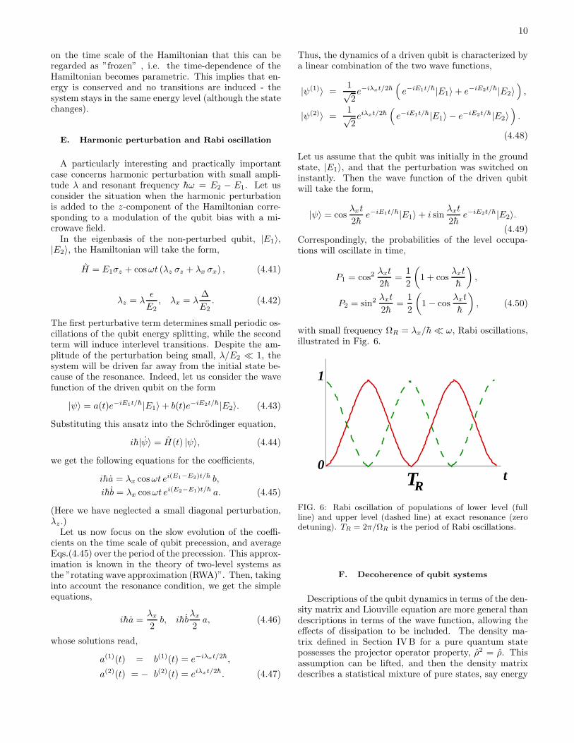
with small frequency ΩR = λx/h≪ ω, Rabi oscillations,illustrated in Fig. 6.

TR

0

1

t

FIG. 6: Rabi oscillation of populations of lower level (fullline) and upper level (dashed line) at exact resonance (zerodetuning). TR = 2π/ΩR is the period of Rabi oscillations.

F. Decoherence of qubit systems

Descriptions of the qubit dynamics in terms of the den-sity matrix and Liouville equation are more general thandescriptions in terms of the wave function, allowing theeffects of dissipation to be included. The density ma-trix defined in Section IVB for a pure quantum statepossesses the projector operator property, ρ2 = ρ. Thisassumption can be lifted, and then the density matrixdescribes a statistical mixture of pure states, say energy

11

eigenstates,

ρ =∑

i

ρi|Ei〉〈Ei|. (4.51)

The density matrix acquires off-diagonal elements whenthe basis rotates away from the energy eigenbasis. Sucha mixed state cannot be represented by the vector on theBloch sphere; however, its evolution is still described bythe Louville equation (4.26),

ih∂tρ = [H, ρ]. (4.52)

The density matrix in Eq. (4.51) is the stationary solu-tion of the Liouville equation. The evolution of an arbi-trary density matrix, off-diagonal in the energy eigenba-sis, is given by the equations,

ρ1, ρ2 = const, ρ12 ∝ ei(E1−E2)t/h. (4.53)

Dissipation is included in the density matrix descrip-tion by extending the qubit Hamiltonian and includinginteraction with an environment. The environment formacroscopic superconducting qubits basically consists ofvarious dissipative elements in external circuits whichprovide bias, control, and measurement of the qubit. The”off-chip” parts of these circuits are usually kept at roomtemperature and produce significant noise. Examples arethe fluctuations in the current source producing magneticfield to bias flux qubits and, similarly, fluctuations of thevoltage source to bias gate of the charge qubits. Elec-tromagnetic radiation from the qubit during operation isanother dissipative mechanisms. There are also intrinsicmicroscopic mechanisms of decoherence, such as fluctuat-ing trapped charges in the substrate of the charge qubits,and fluctuating trapped magnetic flux in the flux qubits,believed to produce dangerous 1/f noise. Another intrin-sic mechanism is possibly the losses in the tunnel junctiondielectric layer. Various kinds of environment are com-monly modelled with an infinite set of linear oscillatorsin thermal equilibrium (thermal bath), linearly coupledto the qubit (Caldeira-Leggett model2,3). The extendedqubit-plus-environment Hamiltonian has the form in thequbit energy eigenbasis82,

H = −1

2Eσz +

∑

i

(λizσz + λi⊥σ⊥)Xi

∑

i

(

P 2i

2m+mω2

iX2i

2

)

, (4.54)

where E = E1 − E2. The physical effects of the twocoupling terms in Eq. (4.54) are quite different. The”transverse” coupling term proportional to λ⊥ inducesinterlevel transitions and eventually leads to the relax-ation. The ”longitudinal” coupling term proportional toλz commutes with the qubit Hamiltonian and thus doesnot induce interlevel transitions. However, it randomlychanges the level spacing, which eventually leads to theloss of phase coherence, dephasing. The effect of both

processes, relaxation and dephasing, are referred to asdecoherence.

Coupling to the environment leads, in the simplestcase, to the following modification of the Liouvilleequation83,84,

∂tρz = − 1

T1(ρz − ρ(0)

z ), (4.55)

∂tρ12 =i

hE ρ12 −

1

T2ρ12 . (4.56)

This equation is known as the Bloch-Redfield equa-tion. The first equation describes relaxation of the

level population to the equilibrium form, ρ(0)z =

−(1/2) tanh(E/2kT ), T1 being the relaxation time. Thesecond equation describes disappearance of the off-diagonal matrix element during characteristic time T2,dephasing.

The relaxation time is determined by the spectral den-sity of the environmental fluctuations at the qubit fre-quency,

1

T1=λ2⊥2Sφ(ω = E). (4.57)

The particular form of the spectral density depends onthe properties of the environment, which are frequentlyexpressed via the impedance (response function) of theenvironment. The most common environment consistsof a pure resistance, in this case, Sφ(ω) ∝ ω, at lowfrequencies.

The dephasing time consists of two parts,

1

T2=

1

2T1+

1

Tφ. (4.58)

The first part is generated by the relaxation process,while the second part results from the pure dephasing dueto the longitudinal coupling to the environment. Thispure dephasing part is proportional to the spectral den-sity of the fluctuation at zero frequency.

1

Tφ=λ2

z

2Sφ(ω = 0). (4.59)

There is already a vast recent literature on de-coherence and noise in superconducting circuits,qubits and detectors, and how to engineer thequbits and environment to minimize decoherence andrelaxation20,42,86,87,88,89,90,91,92,93,94,95,96,97,98,99,100,101,102,103,104,105,106

Many of these issues will be at the focus of this article.

V. CLASSICAL SUPERCONDUCTINGCIRCUITS

In this section we describe a number of elementary su-perconducting circuits with tunnel Josephson junctions,

12

U(φ)

φ

IC RJ

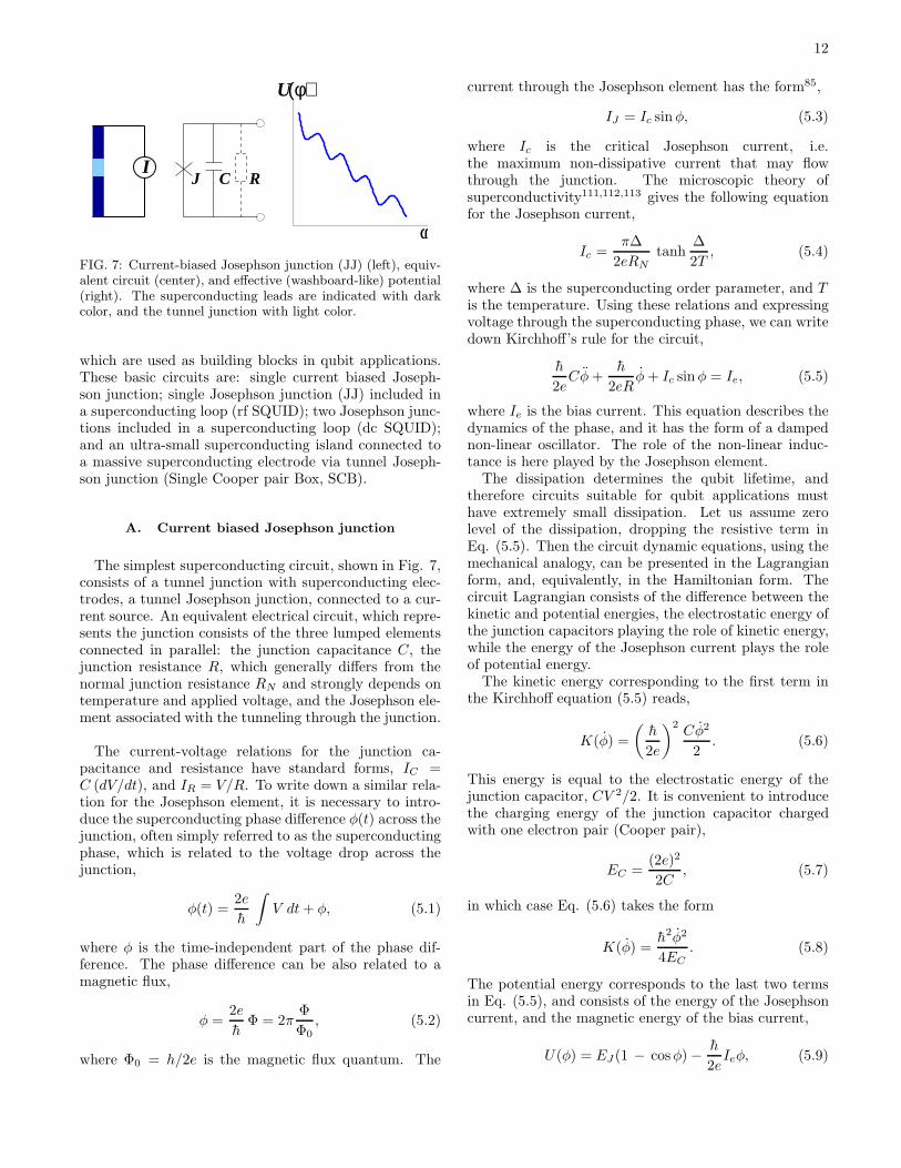
FIG. 7: Current-biased Josephson junction (JJ) (left), equiv-alent circuit (center), and effective (washboard-like) potential(right). The superconducting leads are indicated with darkcolor, and the tunnel junction with light color.

which are used as building blocks in qubit applications.These basic circuits are: single current biased Joseph-son junction; single Josephson junction (JJ) included ina superconducting loop (rf SQUID); two Josephson junc-tions included in a superconducting loop (dc SQUID);and an ultra-small superconducting island connected toa massive superconducting electrode via tunnel Joseph-son junction (Single Cooper pair Box, SCB).

A. Current biased Josephson junction

The simplest superconducting circuit, shown in Fig. 7,consists of a tunnel junction with superconducting elec-trodes, a tunnel Josephson junction, connected to a cur-rent source. An equivalent electrical circuit, which repre-sents the junction consists of the three lumped elementsconnected in parallel: the junction capacitance C, thejunction resistance R, which generally differs from thenormal junction resistance RN and strongly depends ontemperature and applied voltage, and the Josephson ele-ment associated with the tunneling through the junction.

The current-voltage relations for the junction ca-pacitance and resistance have standard forms, IC =C (dV/dt), and IR = V/R. To write down a similar rela-tion for the Josephson element, it is necessary to intro-duce the superconducting phase difference φ(t) across thejunction, often simply referred to as the superconductingphase, which is related to the voltage drop across thejunction,

φ(t) =2e

h

∫

V dt+ φ, (5.1)

where φ is the time-independent part of the phase dif-ference. The phase difference can be also related to amagnetic flux,

φ =2e

hΦ = 2π

Φ

Φ0, (5.2)

where Φ0 = h/2e is the magnetic flux quantum. The

current through the Josephson element has the form85,

IJ = Ic sinφ, (5.3)

where Ic is the critical Josephson current, i.e.the maximum non-dissipative current that may flowthrough the junction. The microscopic theory ofsuperconductivity111,112,113 gives the following equationfor the Josephson current,

Ic =π∆

2eRNtanh

∆

2T, (5.4)

where ∆ is the superconducting order parameter, and Tis the temperature. Using these relations and expressingvoltage through the superconducting phase, we can writedown Kirchhoff’s rule for the circuit,

h

2eCφ+

h

2eRφ+ Ic sinφ = Ie, (5.5)

where Ie is the bias current. This equation describes thedynamics of the phase, and it has the form of a dampednon-linear oscillator. The role of the non-linear induc-tance is here played by the Josephson element.

The dissipation determines the qubit lifetime, andtherefore circuits suitable for qubit applications musthave extremely small dissipation. Let us assume zerolevel of the dissipation, dropping the resistive term inEq. (5.5). Then the circuit dynamic equations, using themechanical analogy, can be presented in the Lagrangianform, and, equivalently, in the Hamiltonian form. Thecircuit Lagrangian consists of the difference between thekinetic and potential energies, the electrostatic energy ofthe junction capacitors playing the role of kinetic energy,while the energy of the Josephson current plays the roleof potential energy.

The kinetic energy corresponding to the first term inthe Kirchhoff equation (5.5) reads,

K(φ) =

(

h

2e

)2Cφ2

2. (5.6)

This energy is equal to the electrostatic energy of thejunction capacitor, CV 2/2. It is convenient to introducethe charging energy of the junction capacitor chargedwith one electron pair (Cooper pair),

EC =(2e)2

2C, (5.7)

in which case Eq. (5.6) takes the form

K(φ) =h2φ2

4EC. (5.8)

The potential energy corresponds to the last two termsin Eq. (5.5), and consists of the energy of the Josephsoncurrent, and the magnetic energy of the bias current,

U(φ) = EJ (1 − cosφ) − h

2eIeφ, (5.9)

13

where EJ = h/2e Ic is the Josephson energy. This po-tential energy has a form of a washboard (see Fig. 7). Inthe absence of bias current this potential corresponds toa pendulum with the frequency of small-amplitude oscil-lations given by

ωJ =

√

2eIchC

. (5.10)

This frequency is known as the plasma frequency of theJosephson junction. When current bias is applied, thependulum potential becomes tilted, its minima becom-ing more shallow, and finally disappearing when the biascurrent becomes equal to the critical current, Ie = IC .At this point, the plasma oscillations become unstable,which physically corresponds to switching to the dissipa-tive regime and the voltage state.

Now we are ready to write down the Lagrangian forthe circuit, which is the difference between the kineticand potential energies. Combining Eqs. (5.8) and (5.9),we get,

L(φ, φ) =h2φ2

4EC− EJ(1 − cosφ) +

h

2eIeφ. (5.11)

It is straightforward to check that the Kirchhoff equation(5.5) coincides with the dynamic equation following fromthe Lagrangian (5.11), using

d

dt

∂L

∂φ− ∂L

∂φ= 0. (5.12)

It is important to emphasize, that the resistance ofthe junction can only be neglected for low temperatures,and also only for slow time evolution of the phase; boththe temperature and the characteristic frequency must besmall compared to the magnitude of the energy gap in thesuperconductor: T, hω ≪ ∆. The physical reason behindthis constraint concerns the amount of generated quasi-particle excitations in the system: if the constraint isfulfilled, the amount of equilibrium and non-equilibriumexcitations will be exponentially small. Otherwise, thegap in the spectrum will not play any significant role,dissipation becomes large, and the advantage of the su-perconducting state compared to the normal conductingstate will be lost.

B. rf-SQUID

The rf-SQUID is the next important superconductingcircuit. It consists of a tunnel Josephson junction in-serted in a superconducting loop, as illustrated in Fig. 8.This circuit realizes magnetic flux bias for the Josephsonjunction113. To describe this circuit, we introduce thecurrent associated with the inductance L of the leads,

IL =h

2eL(φ− φe), φe =

2e

hΦe (5.13)

ΦL

C

RJ

FIG. 8: Superconducting quantum interference device -SQUID (left) consists of a superconducting loop (dark) in-terrupted by a tunnel junction (light); magnetic flux Φ is sentthrough the loop. Right: equivalent circuit.

(φ)U

0 φFIG. 9: SQUID potential: the full (dark) curve correspondsto integer bias flux (in units of flux quanta), while the dashed(light) curve corresponds to half-integer bias flux.

where Φe is the external magnetic flux threading theSQUID loop. The Kirchhoff rule for this circuit takesthe form

h

2eCφ+

h

2eRφ+ Ic sinφ+

h

2eL(φ− φe) = 0. (5.14)

While neglecting the Josephson tunneling (Ic = 0), thisequation describes a damped linear oscillator of a con-ventional LC-circuit. The resonant frequency is then,

ωLC =1√LC

, (5.15)

and the (weak) damping is γ = 1/RC.In the absence of dissipation, it is straightforward to

write down the Lagrangian of the rf-SQUID,

L(φ, φ) =h2φ2

4EC−EJ (1 − cosφ)−EL

(φ− φe)2

2. (5.16)

The last term in this equation corresponds to the energyof the persistent current circulating in the loop,

EL =Φ2

0

4π2L. (5.17)

The potential energy U(φ) corresponding to the last twoterms in Eq. (5.16) is schetched in Fig. 9.

For bias flux equal to integer number of flux quanta,or φe2πn, the potential energy of the SQUID has one ab-solute minimum at φ = φe. For half integer flux quanta

14

ΦIφ φ21

FIG. 10: dc SQUID consists of two tunnel junctions includedin a superconducting loop; arrows indicate the direction ofthe positive Josephson current.

the potential energy has two degenerate minima, whichcorrespond to the two persistent current states circulat-ing in the SQUID loop in the opposite directions. Thisconfiguration of the potential energy provides the basisfor constructing a persistent-current flux qubit (PCQ).

C. dc SQUID

We now consider consider the circuit shown in Fig. 10consisting of two Josephson junctions coupled in paral-lel to a current source. The new physical feature here,compared to a single current-biased junction, is the de-pendence of the effective Josephson energy of the doublejunction on the magnetic flux threading the SQUID loop.

Let us evaluate the effective Josephson energy. Nowthe circuit has two dynamical variables, superconductingphases, φ1,2 across the two Josephson junctions. Defin-ing phases as shown in the figure, and applying consider-ations from Sections VA and VB we find for the staticJosephson currents,

Ic1 sinφ1 − Ic2 sinφ2 = Ie, (5.18)

where Ie is the biasing current. Let us further assumesmall inductance of the SQUID loop and neglect the mag-netic energy of circulating currents. Then the total volt-age drop over the two junctions is zero, V1 +V2 = 0, andtherefore, φ1 + φ2 = φe, where φe is the biasing phaserelated to biasing magnetic flux. Introducing new vari-ables,

φ± =φ1 ± φ2

2, (5.19)

and taking into account that 2φ+ = φe, we rewrite equa-tion (5.18) on the form,

Ic(φe) sin(φ− + α) = Ie, (5.20)

where

Ic(φe) =√

I2c1 + I2

c2 + Ic1Ic2 cosφe, (5.21)

V

Cg

g

FIG. 11: Single Cooper pair box (SCB): a small supercon-ducting island connected to a bulk superconductor via a tun-nel junction; the island potential is controlled by the gatevoltage Vg.

and

tanα =Ic1 − Ic2Ic1 + Ic2

tanφe

2. (5.22)

For a symmetric SQUID with Ic1 = Ic2, giving α = 0,Eq. (5.20) reduces to the form

2Ic cos(φe/2) sinφ− = Ie. (5.23)

The potential energy generated by Eq. (5.20) has theform,

U(φ) = 2EJ cos

(

φe

2

)

(1 − cosφ−) − h

2eIeφ−, (5.24)

which indeed is similar to the potential energy of a sin-gle current biased junction, Eq. (5.9) and Fig. 9, butwith flux-controlled critical current. This property ofthe SQUID is used in qubit applications for controllingthe Josephson coupling, and also for measuring the qubitflux.

The kinetic energy of the SQUID can readily be writ-ten down noticing that it is associated with the chargingenergy of the two junction capacitances connected in par-allel,

K(φ) =

(

h

2e

)2

(C1 + C2)φ2

2. (5.25)

Thus the Lagrangian for the SQUID has a form similarto Eq. (5.11) where EC = (2e)2/2(C1 + C2),

L(φ, φ) =h2φ2

4EC− 2EJ cos

(

φe

2

)

(1 − cosφ) +h

2eIeφ.

(5.26)

D. Single Cooper Pair Box (SCB)

There is a particularly important Josephson junctioncircuit consisting of a small superconducting island con-nected via a Josephson tunnel junction to a large super-conducting reservoir (see Fig. 11).

15

gV

I

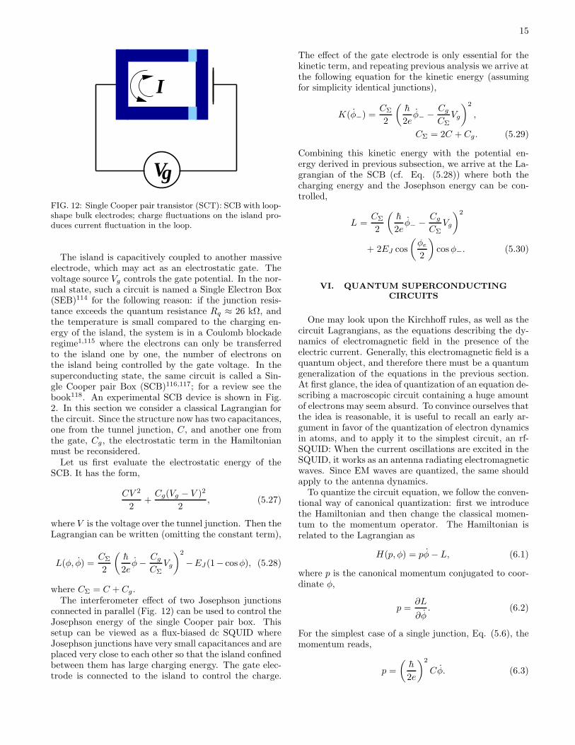
FIG. 12: Single Cooper pair transistor (SCT): SCB with loop-shape bulk electrodes; charge fluctuations on the island pro-duces current fluctuation in the loop.

The island is capacitively coupled to another massiveelectrode, which may act as an electrostatic gate. Thevoltage source Vg controls the gate potential. In the nor-mal state, such a circuit is named a Single Electron Box(SEB)114 for the following reason: if the junction resis-tance exceeds the quantum resistance Rq ≈ 26 kΩ, andthe temperature is small compared to the charging en-ergy of the island, the system is in a Coulomb blockaderegime1,115 where the electrons can only be transferredto the island one by one, the number of electrons onthe island being controlled by the gate voltage. In thesuperconducting state, the same circuit is called a Sin-gle Cooper pair Box (SCB)116,117; for a review see thebook118. An experimental SCB device is shown in Fig.2. In this section we consider a classical Lagrangian forthe circuit. Since the structure now has two capacitances,one from the tunnel junction, C, and another one fromthe gate, Cg, the electrostatic term in the Hamiltonianmust be reconsidered.

Let us first evaluate the electrostatic energy of theSCB. It has the form,

CV 2

2+Cg(Vg − V )2

2, (5.27)

where V is the voltage over the tunnel junction. Then theLagrangian can be written (omitting the constant term),

L(φ, φ) =CΣ

2

(

h

2eφ− Cg

CΣVg

)2

−EJ(1− cosφ), (5.28)

where CΣ = C + Cg.The interferometer effect of two Josephson junctions

connected in parallel (Fig. 12) can be used to control theJosephson energy of the single Cooper pair box. Thissetup can be viewed as a flux-biased dc SQUID whereJosephson junctions have very small capacitances and areplaced very close to each other so that the island confinedbetween them has large charging energy. The gate elec-trode is connected to the island to control the charge.

The effect of the gate electrode is only essential for thekinetic term, and repeating previous analysis we arrive atthe following equation for the kinetic energy (assumingfor simplicity identical junctions),

K(φ−) =CΣ

2

(

h

2eφ− − Cg

CΣVg

)2

,

CΣ = 2C + Cg. (5.29)

Combining this kinetic energy with the potential en-ergy derived in previous subsection, we arrive at the La-grangian of the SCB (cf. Eq. (5.28)) where both thecharging energy and the Josephson energy can be con-trolled,

L =CΣ

2

(

h

2eφ− − Cg

CΣVg

)2

+ 2EJ cos

(

φe

2

)

cosφ−. (5.30)

VI. QUANTUM SUPERCONDUCTINGCIRCUITS

One may look upon the Kirchhoff rules, as well as thecircuit Lagrangians, as the equations describing the dy-namics of electromagnetic field in the presence of theelectric current. Generally, this electromagnetic field is aquantum object, and therefore there must be a quantumgeneralization of the equations in the previous section.At first glance, the idea of quantization of an equation de-scribing a macroscopic circuit containing a huge amountof electrons may seem absurd. To convince ourselves thatthe idea is reasonable, it is useful to recall an early ar-gument in favor of the quantization of electron dynamicsin atoms, and to apply it to the simplest circuit, an rf-SQUID: When the current oscillations are excited in theSQUID, it works as an antenna radiating electromagneticwaves. Since EM waves are quantized, the same shouldapply to the antenna dynamics.

To quantize the circuit equation, we follow the conven-tional way of canonical quantization: first we introducethe Hamiltonian and then change the classical momen-tum to the momentum operator. The Hamiltonian isrelated to the Lagrangian as

H(p, φ) = pφ− L, (6.1)

where p is the canonical momentum conjugated to coor-dinate φ,

p =∂L

∂φ. (6.2)

For the simplest case of a single junction, Eq. (5.6), themomentum reads,

p =

(

h

2e

)2

Cφ. (6.3)

16

The so defined momentum has a simple interpretation:it is proportional to the charge q = CV on the junctioncapacitor, p = (h/2e)q, or the number n of electronicpairs on the junction capacitor,

p = hn. (6.4)

The Hamiltonian for the current-biased junction hasthe form (omitting a constant),

H = EC n2 − EJ cosφ− h

2eIeφ. (6.5)

Similarly, the Hamiltonian for the SQUID circuit has theform

H(n, φ) = ECn2 − EJ cosφ+ EL

(φ− φe)2

2. (6.6)

The dc SQUID considered in the previous Section VChas two degrees of freedom. The Hamiltonian can bewritten by generalizing Eqs. (6.5), (6.6) for the phasesφ±. In the symmetric case we have,

H = EC n2+ + EC n

2− − 2EJ cosφ+ cosφ−

+ EL(2φ+ − φe)

2

2+

h

2eIeφ−. (6.7)

For the SCB, Eq. (5.28), the conjugated momentum hasthe form,

p =hCΣ

2e

(

h

2eφ− Cg

CΣVg

)

, (6.8)

and the Hamiltonian reads,

H = EC(n− ng)2 − EJ cosφ, (6.9)

where now EC = (2e)2/2CΣ, and n = p/h has the mean-ing of the number of electron pairs (Cooper pairs) on theisland electrode. ng = −CgVg/2e is the charge on thegate capacitor (in units of Cooper pairs (2e)), which canbe tuned by the gate potential, and which therefore playsthe role of external controlling parameter.

The quantum Hamiltonian results from Eq. (6.2) bysubstituting the classical momentum p for the differentialoperator,

p = −ih ∂

∂φ. (6.10)

Similarly, one can define the charge operator,

q = − 2ei∂

∂φ, (6.11)

and the operator of the pair number,

n = − i∂

∂φ. (6.12)

The commutation relation between the phase operatorand the pair number operator has a particularly simpleform,

[φ, n] = i. (6.13)

The meaning of the quantization procedure is the fol-lowing: the phase and charge dynamical variables cannot be exactly determined by means of physical measure-ments; they are fundamentally random variables with theprobability of realization of certain values given by themodulus square of the wave function of a particular state,

〈φ〉 =

∫

ψ∗(φ)φψ(φ) dφ, 〈q〉 =

∫

ψ∗(φ) q ψ(φ) dφ.

(6.14)The time evolution of the wave function is given by theSchrodinger equation,

ih∂ψ(φ, t)

∂t= Hψ(φ, t) (6.15)

where H is the circuit quantum Hamiltonian. The ex-plicit form of the quantum Hamiltonian for the circuitsconsidered above, is the following:

rf-SQUID:

H = EC n2 − EJ cosφ+ EL

(φ− φe)2

2; (6.16)

Current biased JJ:

H = EC n2 − EJ cosφ+

h

2eIeφ; (6.17)

dc-SQUID:

H = EC n2+ + EC n

2− − 2EJ cosφ+ cosφ−

+ EL(2φ+ − φe)

2

2+

h

2eIeφ−. (6.18)

and finally the single Cooper pair box (SCB):

H = EC(n− ng)2 − EJ cosφ, (6.19)

For junctions connecting macroscopically large elec-trodes, the charge on the junction capacitor is a con-tinuous variable. This implies that no specific boundaryconditions on the wave function are imposed. The sit-uation is different for the SCB: in this case one of theelectrodes, the island, is supposed to be small enoughto show pronounced charging effects. If tunneling is for-bidden, electrons are trapped on the island, and theirnumber is always integer (the charge quantization con-dition). However, there is a difference between the ener-gies of even and odd numbers of electrons on the island:while an electron pair belongs to the superconductingcondensate and has the additional energy EC , a singleelectron forms an excitation and thus its energy consistsof the charging energy, EC/2 plus the excitation energy,

17

∆ (parity effect)116. To prevent the appearance of indi-vidual electrons on the island and to provide the SCBregime, the condition ∆ ≫ EC/2 must be fulfilled. Thuswhen the tunneling is switched on, only Josephson tun-neling is allowed since it transfers Cooper pairs and thenumber of electrons on the island must change pairwise,n− = integer. In order to provide such a constraint, peri-odic boundary conditions on the SCB wave function areimposed,

ψ(φ) = ψ(φ + 2π). (6.20)

This implies that arbitrary state of the SCB is a super-position of the charge states with integer amount of theCooper pairs,

ψ(φ) =∑

n

aneinφ. (6.21)

The uncertainty of the dynamical variables are not im-portant as long as the relative mean deviations of dy-namical variables are small, i.e. the amplitudes of thequantum fluctuations are small. In this case, the particlebehaves as a classical particle. It is known from quan-tum mechanics, that this corresponds to large mass ofthe particle, in our case, to large junction capacitance.Thus we conclude that the quantum effects in the circuitdynamics are essential when the junction capacitancesare sufficiently small. The qualitative criterion is thatthe charging energy must be larger than, or comparableto, the Josephson energy of the junction, EC ∼ EJ .

Typical Josephson energies of the tunnel junctions inqubit circuits are of the order of a few degrees Kelvinor less. Bearing in mind that the insulating layers ofthe junctions have the thickness of few atomic distances,and modeling the junction as a planar capacitor, the esti-mated junction area should be smaller than a few squaremicrometers to observe the circuit quantum dynamics.

One of most important consequences of the quantumdynamics is quantization of the energy of the circuit. Letus consider, for example, the LC circuit. In the classicalcase, the amplitude of the plasma oscillations has con-tinuous values. In the quantum case the amplitude ofoscillation can only have certain discrete values definedthrough the energy spectrum of the oscillator. The linearoscillator is well studied in the quantum mechanics, andits energy spectrum is very well known,

En = hωLC(n+ 1/2), n = 0, 1, 2, ... (6.22)

One may ask, why is quantum dynamics never ob-served in ordinary electrical circuits? After all, in high-frequency applications, frequencies up to THz are avail-able, which corresponds to a distance between the quan-tized oscillator levels of order 10K, which can be observedat sufficiently low temperature. For an illuminative dis-cussion on this issue see the paper by Martinis, Devoretand Clarke123. According to Ref. 2 it is the dissipationthat kills quantum fluctuations: as known from classi-cal mechanics, the dissipation (normal resistance) broad-ens the resonance, and good resonators must have small

resonance width, γ = 1/RC compared to the resonancefrequency, γ ≪ ωLC . It is intuitively clear that the quan-tization effect will be destroyed when the level broaden-ing exceeds the level spacing. For quantum behavior ofthe circuit, narrow resonances, γ ≪ ωLC , are thereforeessential. However, even in this case it is hard to ob-serve the quantum dynamics in linear circuits such asLC-resonators123 because the expectation values of thelinear oscillator follow the classical time evolution. Thusthe presence of non-linear circuit elements is essential.

The linear oscillator provides the simplest example ofa quantum energy level spectrum: it only consists of dis-crete levels with equal distance between the levels. Thelevel spectrum of the Josephson junction associated witha pendulum potential is more complicated. Firstly, be-cause of the non-linearity (non-parabolic potential wells),the energy spectrum is non-equidistant (anharmonic),the high-energy levels being closer to each other than thelow-energy levels. Moreover, for energies larger than theamplitude of the potential (top of the barrier), EJ , thespectrum is continuous. Secondly, one has to take intoaccount the possibility of a particle tunneling betweenneighboring potential wells: this will produce broadeningof the energy levels into energy bands. The level broad-ening is determined by the overlap of the wave functiontails under the potential barriers, and it must be smallfor levels lying very close to the bottom of the potentialwells. Such a situation may only exist if the level spac-ing, given by the plasma frequency of the tunnel junctionis much smaller than the Josephson energy, hωJ ≪ EJ ,i.e. when EC ≪ EJ . This almost classical regime withJosephson tunneling dominating over charging effects, iscalled the phase regime, because phase fluctuations aresmall and the superconducting phase is well defined. Inthe opposite case, EC ≫ EJ , the lowest energy level lieswell above the potential barrier, and this situation corre-sponds to wide energy bands separated by small energygaps. In this case, the wave function far from the gapedges can be well approximated with a plane wave,

ψq(φ) = expiqφ

2e. (6.23)

This wave function corresponds to an eigenstate of thecharge operator with well defined value of the charge, q.Such a regime with small charge fluctuations is called thecharge regime.

VII. BASIC QUBITS

The quantum superconducting circuits consideredabove contain a large number of energy levels, while forqubit operation only two levels are required. Moreover,these two qubit levels must be well decoupled from theother levels in the sense that transitions between qubitlevels and the environment must be much less probablethan the transitions between the qubit levels itself. Typi-cally that means that the qubit should involve a low-lying

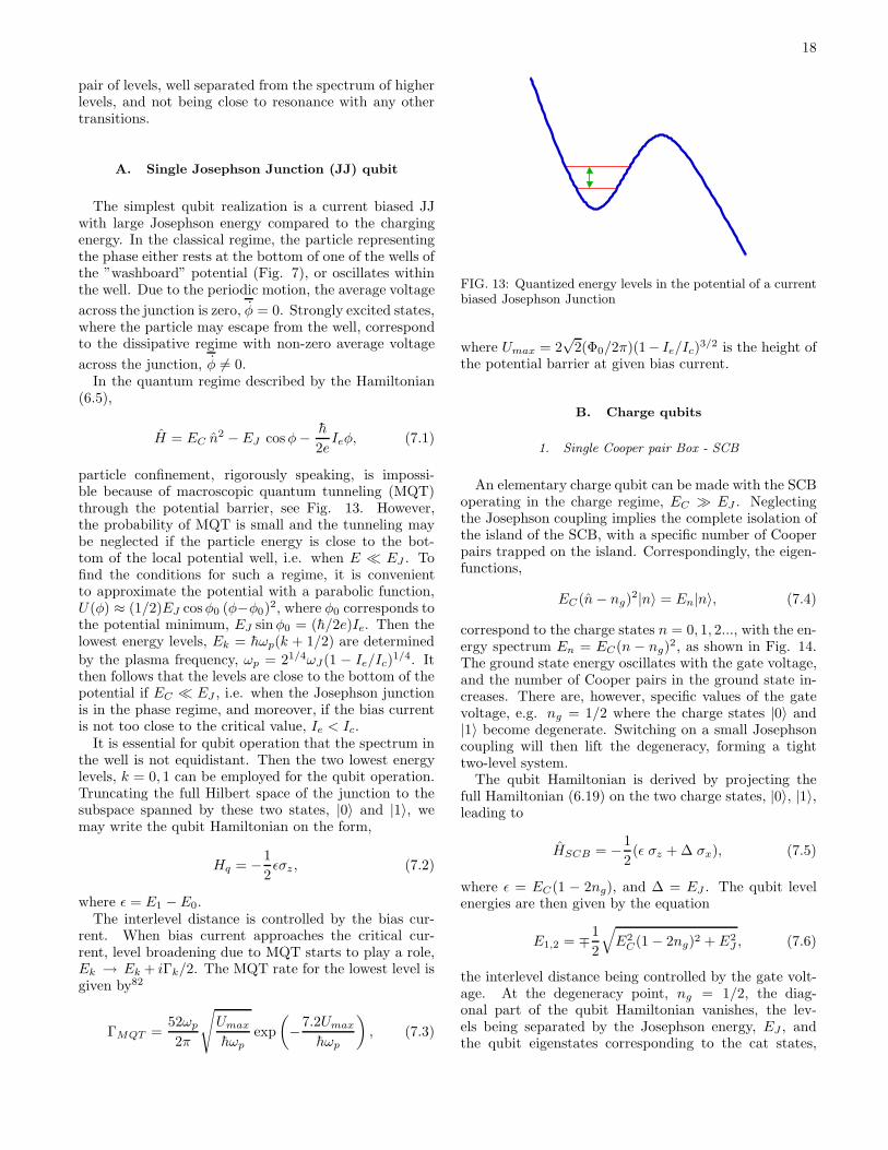
18

pair of levels, well separated from the spectrum of higherlevels, and not being close to resonance with any othertransitions.

A. Single Josephson Junction (JJ) qubit

The simplest qubit realization is a current biased JJwith large Josephson energy compared to the chargingenergy. In the classical regime, the particle representingthe phase either rests at the bottom of one of the wells ofthe ”washboard” potential (Fig. 7), or oscillates withinthe well. Due to the periodic motion, the average voltage

across the junction is zero, φ = 0. Strongly excited states,where the particle may escape from the well, correspondto the dissipative regime with non-zero average voltage

across the junction, φ 6= 0.In the quantum regime described by the Hamiltonian

(6.5),

H = EC n2 − EJ cosφ− h

2eIeφ, (7.1)

particle confinement, rigorously speaking, is impossi-ble because of macroscopic quantum tunneling (MQT)through the potential barrier, see Fig. 13. However,the probability of MQT is small and the tunneling maybe neglected if the particle energy is close to the bot-tom of the local potential well, i.e. when E ≪ EJ . Tofind the conditions for such a regime, it is convenientto approximate the potential with a parabolic function,U(φ) ≈ (1/2)EJ cosφ0 (φ−φ0)

2, where φ0 corresponds tothe potential minimum, EJ sinφ0 = (h/2e)Ie. Then thelowest energy levels, Ek = hωp(k + 1/2) are determined

by the plasma frequency, ωp = 21/4ωJ(1 − Ie/Ic)1/4. It

then follows that the levels are close to the bottom of thepotential if EC ≪ EJ , i.e. when the Josephson junctionis in the phase regime, and moreover, if the bias currentis not too close to the critical value, Ie < Ic.

It is essential for qubit operation that the spectrum inthe well is not equidistant. Then the two lowest energylevels, k = 0, 1 can be employed for the qubit operation.Truncating the full Hilbert space of the junction to thesubspace spanned by these two states, |0〉 and |1〉, wemay write the qubit Hamiltonian on the form,

Hq = −1

2ǫσz , (7.2)

where ǫ = E1 − E0.The interlevel distance is controlled by the bias cur-

rent. When bias current approaches the critical cur-rent, level broadening due to MQT starts to play a role,Ek → Ek + iΓk/2. The MQT rate for the lowest level isgiven by82

ΓMQT =52ωp

2π

√

Umax

hωpexp

(

−7.2Umax

hωp

)

, (7.3)

FIG. 13: Quantized energy levels in the potential of a currentbiased Josephson Junction

where Umax = 2√

2(Φ0/2π)(1− Ie/Ic)3/2 is the height of

the potential barrier at given bias current.

B. Charge qubits

1. Single Cooper pair Box - SCB

An elementary charge qubit can be made with the SCBoperating in the charge regime, EC ≫ EJ . Neglectingthe Josephson coupling implies the complete isolation ofthe island of the SCB, with a specific number of Cooperpairs trapped on the island. Correspondingly, the eigen-functions,

EC(n− ng)2|n〉 = En|n〉, (7.4)

correspond to the charge states n = 0, 1, 2..., with the en-ergy spectrum En = EC(n − ng)

2, as shown in Fig. 14.The ground state energy oscillates with the gate voltage,and the number of Cooper pairs in the ground state in-creases. There are, however, specific values of the gatevoltage, e.g. ng = 1/2 where the charge states |0〉 and|1〉 become degenerate. Switching on a small Josephsoncoupling will then lift the degeneracy, forming a tighttwo-level system.

The qubit Hamiltonian is derived by projecting thefull Hamiltonian (6.19) on the two charge states, |0〉, |1〉,leading to

HSCB = −1

2(ǫ σz + ∆ σx), (7.5)

where ǫ = EC(1 − 2ng), and ∆ = EJ . The qubit levelenergies are then given by the equation

E1,2 = ∓1

2

√

E2C(1 − 2ng)2 + E2

J , (7.6)

the interlevel distance being controlled by the gate volt-age. At the degeneracy point, ng = 1/2, the diag-onal part of the qubit Hamiltonian vanishes, the lev-els being separated by the Josephson energy, EJ , andthe qubit eigenstates corresponding to the cat states,

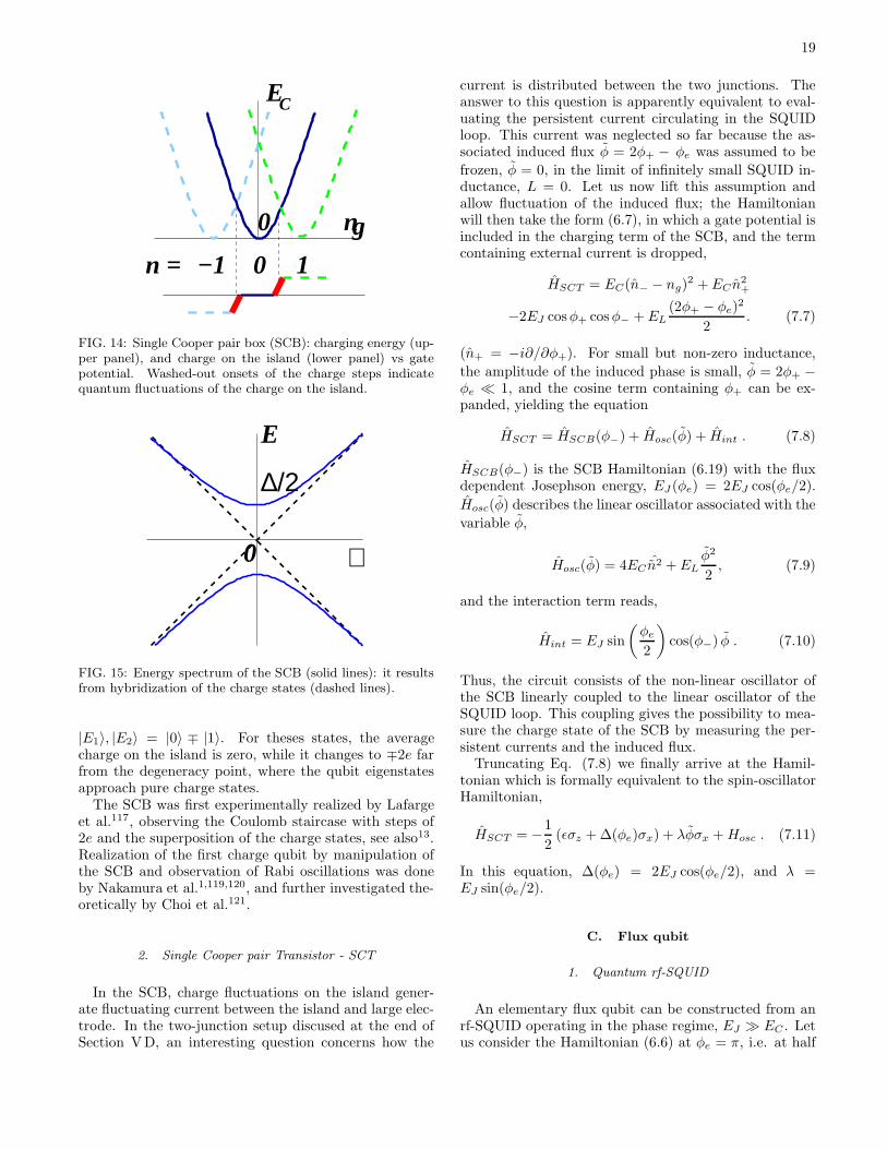
19

E

ng

0n =

0

C

−1 1

FIG. 14: Single Cooper pair box (SCB): charging energy (up-per panel), and charge on the island (lower panel) vs gatepotential. Washed-out onsets of the charge steps indicatequantum fluctuations of the charge on the island.

∋

∆/2

E

0

FIG. 15: Energy spectrum of the SCB (solid lines): it resultsfrom hybridization of the charge states (dashed lines).

|E1〉, |E2〉 = |0〉 ∓ |1〉. For theses states, the averagecharge on the island is zero, while it changes to ∓2e farfrom the degeneracy point, where the qubit eigenstatesapproach pure charge states.

The SCB was first experimentally realized by Lafargeet al.117, observing the Coulomb staircase with steps of2e and the superposition of the charge states, see also13.Realization of the first charge qubit by manipulation ofthe SCB and observation of Rabi oscillations was doneby Nakamura et al.1,119,120, and further investigated the-oretically by Choi et al.121.

2. Single Cooper pair Transistor - SCT

In the SCB, charge fluctuations on the island gener-ate fluctuating current between the island and large elec-trode. In the two-junction setup discused at the end ofSection VD, an interesting question concerns how the

current is distributed between the two junctions. Theanswer to this question is apparently equivalent to eval-uating the persistent current circulating in the SQUIDloop. This current was neglected so far because the as-sociated induced flux φ = 2φ+ − φe was assumed to be

frozen, φ = 0, in the limit of infinitely small SQUID in-ductance, L = 0. Let us now lift this assumption andallow fluctuation of the induced flux; the Hamiltonianwill then take the form (6.7), in which a gate potential isincluded in the charging term of the SCB, and the termcontaining external current is dropped,

HSCT = EC(n− − ng)2 + EC n

2+

−2EJ cosφ+ cosφ− + EL(2φ+ − φe)

2

2. (7.7)

(n+ = −i∂/∂φ+). For small but non-zero inductance,

the amplitude of the induced phase is small, φ = 2φ+ −φe ≪ 1, and the cosine term containing φ+ can be ex-panded, yielding the equation

HSCT = HSCB(φ−) + Hosc(φ) + Hint . (7.8)

HSCB(φ−) is the SCB Hamiltonian (6.19) with the fluxdependent Josephson energy, EJ (φe) = 2EJ cos(φe/2).

Hosc(φ) describes the linear oscillator associated with the

variable φ,

Hosc(φ) = 4ECˆn2 + EL

φ2

2, (7.9)

and the interaction term reads,

Hint = EJ sin

(

φe

2

)

cos(φ−) φ . (7.10)

Thus, the circuit consists of the non-linear oscillator ofthe SCB linearly coupled to the linear oscillator of theSQUID loop. This coupling gives the possibility to mea-sure the charge state of the SCB by measuring the per-sistent currents and the induced flux.

Truncating Eq. (7.8) we finally arrive at the Hamil-tonian which is formally equivalent to the spin-oscillatorHamiltonian,

HSCT = −1

2(ǫσz + ∆(φe)σx) + λφσx +Hosc . (7.11)

In this equation, ∆(φe) = 2EJ cos(φe/2), and λ =EJ sin(φe/2).

C. Flux qubit

1. Quantum rf-SQUID

An elementary flux qubit can be constructed from anrf-SQUID operating in the phase regime, EJ ≫ EC . Letus consider the Hamiltonian (6.6) at φe = π, i.e. at half

20

0∆

E

φ

FIG. 16: Double-well potential of the rf-SQUID with de-generate quantum levels in the wells (black). Macroscopicquantum tunneling (MQT) through the potential barrier in-troduces a level splitting ∆, and the lowest level pair forms aqubit.

0

U(φ)

φ

UlUr

FIG. 17: Flux qubit: truncation of the junction Hamiltonian;dashed lines indicate potentials of the left and right wells withground energy levels.

integer bias magnetic flux. The potential, U(φ), shownin Fig. 16 has two identical wells with equal energy levelswhen MQT between the wells is neglected (phase regime,ωJ ≪ EJ ). These levels are connected with current fluc-tuations within each well around averaged values cor-responding to clockwise and counterclockwise persistentcurrents circulating in the loop (the flux states). Letus consider the lowest, doubly degenerate, energy level.When the tunneling is switched on, the levels split, anda tight two-level system is formed with the level spacingdetermined by the MQT rate, which is much smaller thanthe level spacing in the well. In the case that the tunnel-ing barrier is much smaller than the Josephson energy,the potential in Eq. (5.9) can be approximated,

U(φ) = EJ (1 − cosφ) + EL(φ− φe)

2

2

≈ EL

(

−ε φ2

2− fφ+

1 + ε

24φ4

)

, (7.12)

where φ = φ− π, f = φe − π, and where

ε =EJ

EL− 1 ≪ 1. (7.13)

determines the height of the tunnel barrier.The qubit Hamiltonian is derived by projecting the

whole Hilbert space of the full Hamiltonian (6.6) on the

subspace spanned by these two levels. The starting pointof the truncation procedure is to approximate the doublewell potential with Ul and Ur, as shown in Fig. 17, toconfine the particle to the left or to the right well, respec-tively. The corresponding ground state wave functions |l〉and |r〉 satisfy the stationary Schrodinger equation,

Hl|l〉 = El|l〉, Hr|r〉 = Er|r〉. (7.14)

The averaged induced flux for these states, φl and φr

have opposite signs, manifesting opposite directions ofthe circulating persistent currents. Let us allow the biasflux to deviate slightly from the half integer value, φe =π + f , so that the ground state energies are not equalbut still close to each other, El ≈ Er. The tunneling willhybridize the levels, and we can approximate the trueeigenfunction, |E〉,

H |E〉 = E|E〉, (7.15)

with a superposition,

|E〉 = a|l〉 + b|r〉. (7.16)

The qubit Hamiltonian is given by the matrix elementsof the full Hamiltonian, Eq. (7.15), with respect to thestates |l〉 and |r〉,

Hll = El + 〈l|U − Ul|l〉,Hrr = Er + 〈r|U − Ur|r〉,

Hrl = El〈r|l〉 + 〈r|U − Ul|l〉. (7.17)

In the diagonal matrix elements, the second terms aresmall because the wave functions are exponentially smallin the region where the deviation of the approximatedpotential from the true one is appreciable. The off di-agonal matrix element is exponentially small because ofsmall overlap of the ground state wave functions in theleft and right wells, and also here the main contributioncomes from the first term. Since the wave functions canbe chosen real, the truncated Hamiltonian is symmet-ric, Hlr = Hrl. Then introducing ǫ = Er − El, and∆/2 = Hrl, we arrive at the Hamiltonian of the fluxqubit,

H = −1

2(ǫσz + ∆σx). (7.18)

The Hamiltonian of the flux qubit is formally equiva-lent to that of the charge qubit, Eq. (7.5), but the phys-ical meaning of the terms is rather different. The fluxqubit Hamiltonian is written in the flux basis, i.e. thebasis of the states with certain averaged induced flux, φl

and φr (rather than the charge basis of the charge qubit).The energy spectrum of the flux qubit is obviously the

same as that of the charge qubit,

E1,2 = ∓1

2

√

ǫ2 + ∆2, (7.19)

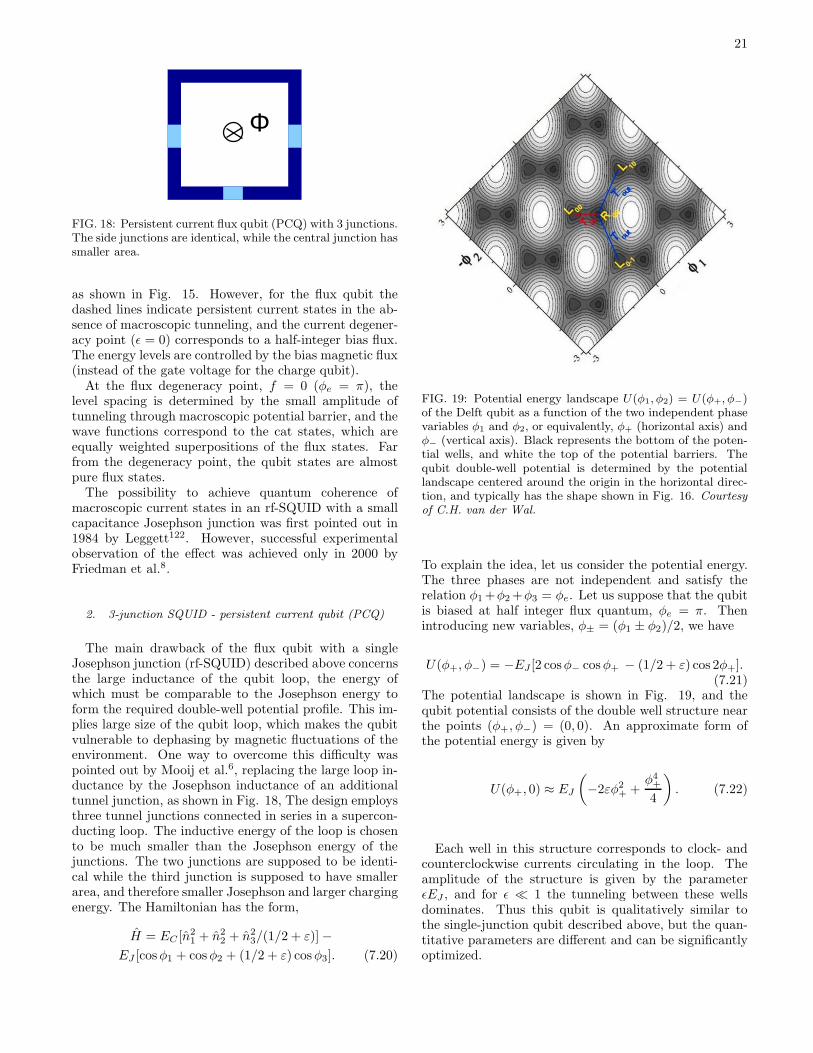
21

Φ

FIG. 18: Persistent current flux qubit (PCQ) with 3 junctions.The side junctions are identical, while the central junction hassmaller area.

as shown in Fig. 15. However, for the flux qubit thedashed lines indicate persistent current states in the ab-sence of macroscopic tunneling, and the current degener-acy point (ǫ = 0) corresponds to a half-integer bias flux.The energy levels are controlled by the bias magnetic flux(instead of the gate voltage for the charge qubit).

At the flux degeneracy point, f = 0 (φe = π), thelevel spacing is determined by the small amplitude oftunneling through macroscopic potential barrier, and thewave functions correspond to the cat states, which areequally weighted superpositions of the flux states. Farfrom the degeneracy point, the qubit states are almostpure flux states.

The possibility to achieve quantum coherence ofmacroscopic current states in an rf-SQUID with a smallcapacitance Josephson junction was first pointed out in1984 by Leggett122. However, successful experimentalobservation of the effect was achieved only in 2000 byFriedman et al.8.

2. 3-junction SQUID - persistent current qubit (PCQ)

The main drawback of the flux qubit with a singleJosephson junction (rf-SQUID) described above concernsthe large inductance of the qubit loop, the energy ofwhich must be comparable to the Josephson energy toform the required double-well potential profile. This im-plies large size of the qubit loop, which makes the qubitvulnerable to dephasing by magnetic fluctuations of theenvironment. One way to overcome this difficulty waspointed out by Mooij et al.6, replacing the large loop in-ductance by the Josephson inductance of an additionaltunnel junction, as shown in Fig. 18, The design employsthree tunnel junctions connected in series in a supercon-ducting loop. The inductive energy of the loop is chosento be much smaller than the Josephson energy of thejunctions. The two junctions are supposed to be identi-cal while the third junction is supposed to have smallerarea, and therefore smaller Josephson and larger chargingenergy. The Hamiltonian has the form,

H = EC [n21 + n2

2 + n23/(1/2 + ε)] −

EJ [cosφ1 + cosφ2 + (1/2 + ε) cosφ3]. (7.20)

FIG. 19: Potential energy landscape U(φ1, φ2) = U(φ+, φ−)of the Delft qubit as a function of the two independent phasevariables φ1 and φ2, or equivalently, φ+ (horizontal axis) andφ− (vertical axis). Black represents the bottom of the poten-tial wells, and white the top of the potential barriers. Thequbit double-well potential is determined by the potentiallandscape centered around the origin in the horizontal direc-tion, and typically has the shape shown in Fig. 16. Courtesyof C.H. van der Wal.

To explain the idea, let us consider the potential energy.The three phases are not independent and satisfy therelation φ1 +φ2 +φ3 = φe. Let us suppose that the qubitis biased at half integer flux quantum, φe = π. Thenintroducing new variables, φ± = (φ1 ± φ2)/2, we have

U(φ+, φ−) = −EJ [2 cosφ− cosφ+ − (1/2 + ε) cos 2φ+].(7.21)

The potential landscape is shown in Fig. 19, and thequbit potential consists of the double well structure nearthe points (φ+, φ−) = (0, 0). An approximate form ofthe potential energy is given by

U(φ+, 0) ≈ EJ

(

−2εφ2+ +

φ4+

4

)

. (7.22)

Each well in this structure corresponds to clock- andcounterclockwise currents circulating in the loop. Theamplitude of the structure is given by the parameterǫEJ , and for ǫ ≪ 1 the tunneling between these wellsdominates. Thus this qubit is qualitatively similar tothe single-junction qubit described above, but the quan-titative parameters are different and can be significantlyoptimized.

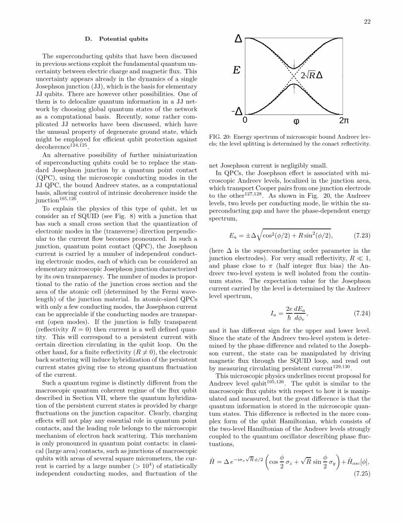
22

D. Potential qubits

The superconducting qubits that have been discussedin previous sections exploit the fundamental quantum un-certainty between electric charge and magnetic flux. Thisuncertainty appears already in the dynamics of a singleJosephson junction (JJ), which is the basis for elementaryJJ qubits. There are however other possibilities. One ofthem is to delocalize quantum information in a JJ net-work by choosing global quantum states of the networkas a computational basis. Recently, some rather com-plicated JJ networks have been discussed, which havethe unusual property of degenerate ground state, whichmight be employed for efficient qubit protection againstdecoherence124,125.

An alternative possibility of further miniaturizationof superconducting qubits could be to replace the stan-dard Josephson junction by a quantum point contact(QPC), using the microscopic conducting modes in theJJ QPC, the bound Andreev states, as a computationalbasis, allowing control of intrinsic decoherence inside thejunction105,126.

To explain the physics of this type of qubit, let usconsider an rf SQUID (see Fig. 8) with a junction thathas such a small cross section that the quantization ofelectronic modes in the (transverse) direction perpendic-ular to the current flow becomes pronounced. In such ajunction, quantum point contact (QPC), the Josephsoncurrent is carried by a number of independent conduct-ing electronic modes, each of which can be considered anelementary microscopic Josephson junction characterizedby its own transparency. The number of modes is propor-tional to the ratio of the junction cross section and thearea of the atomic cell (determined by the Fermi wave-length) of the junction material. In atomic-sized QPCswith only a few conducting modes, the Josephson currentcan be appreciable if the conducting modes are transpar-ent (open modes). If the junction is fully transparent(reflectivity R = 0) then current is a well defined quan-tity. This will correspond to a persistent current withcertain direction circulating in the qubit loop. On theother hand, for a finite reflectivity (R 6= 0), the electronicback scattering will induce hybridization of the persistentcurrent states giving rise to strong quantum fluctuationof the current.

Such a quantum regime is distinctly different from themacroscopic quantum coherent regime of the flux qubitdescribed in Section VII, where the quantum hybridiza-tion of the persistent current states is provided by chargefluctuations on the junction capacitor. Clearly, chargingeffects will not play any essential role in quantum pointcontacts, and the leading role belongs to the microscopicmechanism of electron back scattering. This mechanismis only pronounced in quantum point contacts: in classi-cal (large area) contacts, such as junctions of macroscopicqubits with areas of several square micrometers, the cur-rent is carried by a large number (> 104) of statisticallyindependent conducting modes, and fluctuation of the

0 1 2−1

0

1

E 2

0 2π∆

φ

∆

R ∆

FIG. 20: Energy spectrum of microscopic bound Andreev lev-els; the level splitting is determined by the conact reflectivity.

net Josephson current is negligibly small.In QPCs, the Josephson effect is associated with mi-

croscopic Andreev levels, localized in the junction area,which transport Cooper pairs from one junction electrodeto the other127,128. As shown in Fig. 20, the Andreevlevels, two levels per conducting mode, lie within the su-perconducting gap and have the phase-dependent energyspectrum,

Ea = ±∆

√

cos2(φ/2) +R sin2(φ/2), (7.23)

(here ∆ is the superconducting order parameter in thejunction electrodes). For very small reflectivity, R ≪ 1,and phase close to π (half integer flux bias) the An-dreev two-level system is well isolated from the contin-uum states. The expectation value for the Josephsoncurrent carried by the level is determined by the Andreevlevel spectrum,

Ia =2e

h

dEa

dφe, (7.24)

and it has different sign for the upper and lower level.Since the state of the Andreev two-level system is deter-mined by the phase difference and related to the Joseph-son current, the state can be manipulated by drivingmagnetic flux through the SQUID loop, and read outby measuring circulating persistent current129,130.

This microscopic physics underlines recent proposal forAndreev level qubit105,126. The qubit is similar to themacroscopic flux qubits with respect to how it is manip-ulated and measured, but the great difference is that thequantum information is stored in the microscopic quan-tum states. This difference is reflected in the more com-plex form of the qubit Hamiltonian, which consists ofthe two-level Hamiltonian of the Andreev levels stronglycoupled to the quantum oscillator describing phase fluc-tuations,

H = ∆ e−iσx

√R φ/2

(

cosφ

2σz +

√R sin

φ

2σy

)

+Hosc[φ],

(7.25)

23

Hosc[φ] = EC n+(EL/2)(φ−φe)2. Comparing this equa-

tion with e.g. the SCT Hamiltonian (7.8), we find thatthe truncated Hamiltonian of the SCB is replaced hereby the Andreev level Hamiltonian.

VIII. QUBIT READOUT AND MEASUREMENTOF QUANTUM INFORMATION

In this section we present a number of proposed, andrealized, schemes for measuring quantum states of vari-ous superconducting qubits.

A. Readout: why, when and how?

As already mentioned in Section III D, the ultimateobjective of a qubit readout device is to distinguish theeigenstates of a qubit in a single measurement ”withoutdestroying the qubit”, a so called ”single-shot” quantumnon-demolition (QND) projective measurement. Thisobjective is essential for several reasons: state prepara-tion for computation, readout for error correction duringthe calculation, and readout of results at the end of thecalculation. Strictly speaking, the QND property is onlyneeded if the qubit must be left in an eigenstate afterthe readout. In a broader sense, readout of a specificqubit must of course not destroy any other qubits in thesystem.

It must be carefully noted that one cannot ”read outthe state of a qubit” in a single measurement - this is pro-hibited by quantum mechanics. It takes repeated mea-surements on a large number of replicas of the quantumstate to characterize the state of the qubit (Eq. (3.1)) -”quantum tomography”131.

The measurement connects the qubit with the opensystem of the detector, which collapses the combined sys-tem of qubit and measurement device to one of its com-mon eigenstates. If the coupling between the qubit andthe detector is weak, the eigenstates are approximatelythose of the qubit. In general however, one must con-sider the eigenstates of the total qubit-detector systemand manipulate gate voltages and fluxes such that thereadout measurement is performed in a convenient en-ergy eigenbasis (see e.g.42,79).

Even under ideal conditions, a single-shot measure-ment can only determine the population of an eigenstateif the system is prepared in an eigenstate: then the an-swer will always be either ”0” or ”1”. If an ideal single-shot measurement is used to read out a qubit superpo-sition state, e.g. during Rabi oscillation, then again theanswer can only be ”0” or ”1”. To determine the qubitpopulation (i.e. the |a1|2 and |a2|2 probabilities) requiresrepetition of the measurement to obtain the expectationvalue. During the intermediate stages of quantum com-putation one must therefore not perform a measurementon a qubit unless one knows, because of the design andtiming of the algorithm, that this qubit is in an energy

FIG. 21: Measurement of the phase qubit. Long-living levelsform the qubit, while the dashed line indicates a leaky levelwith large energy.

eigenstate. Then the value is predetermined and thequbit left in the eigenstate (Stern-Gerlach-style).

On the other hand, to extract the desired final result itmay be necessary to create an ensemble of calculations tobe able to perform a complete measurement to determinethe expectation values of variables of interest, performingquantum state tomography131.

B. Direct qubit measurement

Direct destructive measurement of the qubit can be il-lustrated with the example of a single JJ (phase) qubit,Section VII A. After the manipulation has been per-formed (e.g. Rabi oscillation), the qubit is left in a su-perposition of the upper and lower energy states. Todetermine the probability of the upper state, one slowlyincreases the bias current until it reaches such a valuethat the upper energy level equals Or gets close to) thetop of the potential barrier, see Fig. 21. Then the junc-tion, being at the upper energy level, will switch from theJosephson branch to the dissipative branch, and this canbe detected by measuring the finite average voltage ap-pearing across the junction (voltage state). If the qubitis in the lower energy state the qubit will remain on theJosephson branch and a finite voltage will not be de-tected (zero-voltage state). An alternative method toactivate switching30 is to apply an rf signal with reso-nant frequency (instead of tilting the junction potential)in order to excite the upper energy level and to induce theswitching event, see Fig. 21 (also illustrating a standardreadout method in atomic physics).

It is obvious that, in this example, the qubit upperenergy state is always destroyed by the measurement.Single-shot measurement is possible provided the MQTrate for the lower energy level is sufficiently small toprevent the junction switching during the measurementtime. It is also essential to keep a sufficiently small rate ofinterlevel transitions induced by fluctuations of the bias

24

Vg

SCB

SET

FIG. 22: Single Electron Transistor (SET) capacitively cou-pled to an SCB.

current and by the current ramping.A similar kind of direct destructive measurement was

performed by Nakamura et al.1 to detect the state of thecharge qubit. The qubit operation was performed at thecharge degeneracy point, ug = 1, where the level splittingis minimal. An applied gate voltage then shifted the SCBworking point (Fig. 15), inducing a large level splittingof the pure charge states |0〉 and |1〉 (the measurementpreparation stage). In this process the upper |1〉 chargestate went above the threshold for Cooper pair decay,creating two quasi-particles which immediately tunnelout via the probe junction into the leads. These quasi-particles were measured as a contribution to the classicalcharge current by repeating the experiment many times.Obviously, this type of measurement is also destructive.

C. Measurement of charge qubit with SET

Non-destructive measurement of the charge qubit hasbeen implemented by connecting the qubit capacitivelyto a SET electrometer69. The idea of this method is touse a qubit island as an additional SET gate (Fig. 22),controlling the dc current through the SET dependingon the state of the qubit. When the measurement is tobe performed, a driving voltage is applied to the SET,and the dc current is measured. Another version of themeasurement procedure is to apply rf bias to the SET(rf-SET69,133,134,135) in Fig. 22, and to measure the dis-sipative or inductive response. In both cases the trans-missivity will show two distinct values correlated withthe two states of the qubit. Yet another version has re-cently been developed by the NEC group136 to performsingle-shot readout: the Cooper pair on the SCB islandthen tunnels out onto a trap island (instead of the leads)used as a gate to control the current through the SET.

The physics of the SET-based readout has been exten-sively studied theoretically (see42,137,138 and referencestherein). A similar idea of controlling the transmissionof a quantum point contact (QPC) (instead of an SET)

t << t ms t < t ms t = t ms

t I(n )x0 t I(n )x

1

P

0 m

FIG. 23: Probability distributions P of counted electrons asfunctions of time after the turning on the measurement beamof electrons. Courtesy of G. Johansson, Chalmers.

capacitively coupled to a charge qubit has also been ex-tensively discussed in literature132,139,140,141,142,143,144.

The induced charge on the SET gate depends on thestate of the qubit, affecting the SET working pointand determining the conductivity and the average cur-rent. The development of the probability distributionsof counted electrons with time is shown in Fig. 23.

As the number of counted electrons grows, the distribu-tions separate and become distinguishable, the distancebetween the peaks developing as ∼ N and the width∼

√N . Detailed investigations144 show that the two

electron-number probability distributions correlate withthe probability of finding the qubit in either of two energylevels. The long-time development depends on the inten-sity and frequency distribution of the back-action noisefrom the electron current. With very weak detector backaction, the qubit can relax to |0〉 during the natural re-laxation time T1. With very strong back-action noise atthe qubit frequency, the qubit may become saturated ina 50/50 mixed state.

D. Measurement via coupled oscillator

Another method of qubit read out that has attractedmuch attention concerns the measurement of the proper-ties of a linear or non-linear oscillator coupled to a qubit.This method is employed for the measurement of inducedmagnetic flux and persistent current in the loop of fluxqubits and charge-phase qubits, as well as for charge mea-surement on charge qubits. With this method, the qubitaffects the characteristics of the coupled oscillator, e.g.changes the shape of the oscillator potential, after whichthe oscillator can be probed to detect the changes. Thereare two versions of the method: resonant spectroscopy ofa linear tank circuit/cavity, and threshold detection us-ing biased JJ or SQUID magnetometer.

The first method uses the fact that the resonance fre-quency of a linear oscillator weakly coupled to the qubitundergoes a shift depending on the qubit state. Theeffect is most easily explained by considering the SCTHamiltonian, Eq. (11.1),

HSCT = −1

2(ǫσz + ∆(φe)σx) + λ(φe)φσx

+4ECˆn2 +

1

2ELφ

2. (8.1)

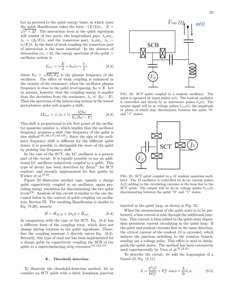
25

Let us proceed to the qubit energy basis, in which caseethe qubit Hamiltonian takes the form −(E/2)σz, E =√ǫ2 + ∆2. The interaction term in the qubit eigenbasis

will consist of two parts, the longitudinal part, λzφσz,λz = (∆/E)λ, and the transverse part, λxφσx, λx =(ǫ/E)λ. In the limit of weak coupling the transverse partof interaction is the most essential. In the absence ofinteraction (φe = 0), the energy spectrum of the qubit +oscillator system is

En∓ = ∓E2

+ hω(n+1

2), (8.2)

where hω =√

8ECEL is the plasma frequency of theoscillator. The effect of weak coupling is enhanced inthe vicinity of the resonance, when the oscillator plasmafrequency is close to the qubit level spacing, hω ≈ E. Letus assume, however, that the coupling energy is smallerthan the deviation from the resonance, λx ≪ |hω − E|.Then the spectrum of the interacting system in the lowestperturbative order will acquire a shift,

δEn± = ± (n+ 1)λ2

xhω

EL(hω − E). (8.3)

This shift is proportional to the first power of the oscilla-tor quantum number n, which implies that the oscillatorfrequency acquires a shift (the frequency of the qubit isalso shifted145,146,147,148,149). Since the sign of the oscil-lator frequency shift is different for the different qubitstates, it is possible to distinguish the state of the qubitby probing this frequency shift.

In the case of the SCT, the LC oscillator is a genericpart of the circuit. It is equally possible to use an addi-tional LC oscillator inductively coupled to a qubit. Thistype of device has been described by Zorin71 for SCTreadout, and recently implemented for flux qubits byIl’ichev et al.27,39.

Figure 24 illustrates another case, namely a chargequbit capacitively coupled to an oscillator, again pro-viding energy resolution for discriminating the two qubitlevels150. Analysis of this circuit is similar to the one dis-cussed below in the context of qubit coupling via oscilla-tors, Section IX. The resulting Hamiltonian is similar toEq. (9.20), namely,

H = HSCB + λσyφ+ Hosc. (8.4)

In comparison with the case of the SCT, Eq. (8.4) hasa different form of the coupling term, which does notchange during rotation to the qubit eigenbasis. There-fore the coupling constant λ directly enters Eq. (8.3).Recently, this type of read out has been implemented fora charge qubit by capacitively coupling the SCB of thequbit to a superconducting strip resonator151,152,153.

E. Threshold detection

To illustrate the threshold-detection method, let usconsider an SCT qubit with a third Josephson junction

Vg

SCB

u(t)Vout (t)

FIG. 24: SCT qubit coupled to a readout oscillator. Thequbit is operated by input pulses u(t). The readout oscillatoris controlled and driven by ac microwave pulses Vg(t). Theoutput signal will be ac voltage pulses Vout(t), the amplitudeor phase of which may discriminate between the qubit ”0”and ”1” states.

SCT Ib

VgVg

FIG. 25: SCT qubit coupled to a JJ readout quantum oscil-lator. The JJ oscillator is controlled by dc/ac current pulsesIb(t) adding to the circulating currents in the loop due to theSCT qubit. The output will be dc/ac voltage pulses Vout(t)discriminating between the qubit ”0” and ”1” states.

inserted in the qubit loop, as shown in Fig. 25.

When the measurement of the qubit state is to be per-formed, a bias current is sent through the additional junc-tion. This current is then added to the qubit-state depen-dent persistent current circulating in the qubit loop. Ifthe qubit and readout currents flow in the same direction,the critical current of the readout JJ is exceeded, whichinduces the junction switching to the resistive branch,sending out a voltage pulse. This effect is used to distin-guish the qubit states. The method has been extensivelyused experimentally by Vion et al.21,22,23.

To describe the circuit, we add the Lagrangian of abiased JJ, Eq. (5.11),

L =h2φ2

4EmC

+ EmJ cosφ+

h

2eIeφ, (8.5)

26

to the SCT Lagrangian (generalized Eq. (5.30), cf. Eqs.(6.7), (7.7)),

LSCT =h2

4EC

(

φ− − 2eCg

hCΣVg

)2

+h2

4ECφ2

+

−2EJ cosφ+ cosφ− − 1

2ELφ

2 (8.6)

(here we have neglected a small contribution of the gatecapacitance to the qubit charging energy). The phase

quantization condition will now read: 2φ+ + φ = φe + φ.The measurement junction will be assumed in the phaseregime, Em

J ≫ EmC , and moreover, the inductive energy

will be the largest energy in the circuit, EL ≫ EmJ . The

latter implies that the induced phase is negligibly smalland can be dropped from the phase quantization condi-tion. We also assume that φe = 0, thus 2φ+ + φ = 0.Then, after having omitted the variable φ+, the kineticenergy term of the qubit can be combined with the muchlarger kinetic energy of the measurement junction lead-ing to insignificant renormalization of the measurementjunction capacitance, Cm +C/4 → Cm. As a result, thetotal Hamiltonian of the circuit will take the form,

H = EC(n− − ng)2 − 2EJ cos

(

φ

2

)

cosφ−

+EmC n2 − Em

J cosφ− h

2eIeφ. (8.7)

Since the measurement junction is supposed to be almostclassical, its phase is fairly close to the minimum of thejunction potential. During qubit operation, the bias cur-rent is zero; hence the phase of the measurement junctionis zero. When the measurement is made, the current isramped to a large value close to the critical current ofthe measurement junction, Ie = (2e/h)Em

J − δI, tiltingthe junction potential and shifting the minimum towardsπ/2. Introducing a new variable φ = π + θ, we expandthe potential with respect to small θ ≪ 1 and, truncatingthe qubit part, we obtain

H = − ǫ

2σz − ∆

2

(

1 − θ

2

)

σx

+EmC n2 − Em

J

θ3

6+

h

2eδI θ, (8.8)

where ∆ = 2√EJ . The ramping is supposed to be adi-

abatic so that the phase remains at the minimum point.Let us analyze the behavior of the potential minimumby omitting a small kinetic term and diagonalizing theHamiltonian (8.8). The corresponding eigenenergies de-pend on θ,

E±(θ) = ∓E2− Em

J

θ3

6+

(

h

2eδI ± ∆2

4E

)

θ, (8.9)

as shown in Fig. 26. Then within the interval of the biascurrents, |δI| ≤ −(2e/h)(∆2/4E), the potential energycorresponding to the ground state has a local minimum,

θ

U

FIG. 26: Josephson potential energy of the measurementjunction during the measurement: for the ”0” qubit eigen-state there is a well (full line) confining a level, while for the”1” qubit state there is no well (dashed line).

while for the excited state it does not. This implies thatwhen the junction is in the ground state, no voltage willbe generated. However, if the junction is in the excitedstate, it will switch to the resistive branch, generating avoltage pulse that can be detected.

With the discussed setup the direction of the persis-tent current is measured. It is also possible to arrangethe measurement of the flux by using a dc SQUID as athreshold detector. Such a setup is suitable for the mea-surement of flux qubits. Let us consider, for example, thethree junction flux qubit from Section VII C inductivelycoupled to a dc SQUID. Then, under certain assump-tions, the Hamiltonian of the system can be reduced tothe following form:

H = −1

2(ǫσz + ∆σx)

+EsC n2 − (Es

J + λσz) cosφ− h

2eδI φ, (8.10)

where EsJ is an effective (bias flux dependent) Josephson

energy of the SQUID, Eq. (5.24), and λ is an effectivecoupling constant proportional to the mutual inductanceof the qubit and the SQUID loops.

IX. PHYSICAL COUPLING SCHEMES FORTWO QUBITS

A. General principles

A generic scheme for coupling qubits is based onthe physical interaction of linear and non-linear os-cillators constituting a superconducting circuit. TheHamiltonians for the SCB, rf-SQUID, and plain JJ con-tain quadratic terms representing the kinetic and poten-tial energies plus the non-linear Josephson energy term,which is quadratic when expanded to lowest order,

H = EC(n− ng)2 + EJ(1 − cosφ) (9.1)

27

FIG. 27: Fixed inductive (flux) coupling of elementary fluxqubit. The loops can be separate, or have a common leg likein the figure.

H = EC n2 + EJ (1 − cosφ) + EL

(φ− φe)2

2(9.2)

H = EC n2 + EJ (1 − cosφ) +

h

2eIeφ. (9.3)

In a multi-qubit system the induced gate charge in theSCB, or the flux through the SQUID loop, or the phasein the Josephson energy, will be a sum of contributionsfrom several (in principle, all) qubits. The energy of thesystem can therefore not be described as the sum of twoindependent qubits because of the quadratic dependence,and the cross terms represent interaction energies of dif-ferent kinds: capacitive, inductive and phase/current.Moreover, using JJ circuits as non-linear coupling ele-ments we have the advantage that the direct physicalcoupling strength may be controlled, e.g tuning the in-ductance via current biased JJs, or tuning the capaci-tance by a voltage biased SCB.

B. Inductive coupling of flux qubits

A common way of coupling flux qubits is the inductivecoupling: magnetic flux induced by one qubit threadsthe loop of another qubit, changing the effective externalflux. This effect is taken into account by introducing theinductance matrix Lik, which connects flux in the i-thloop with the current circulating in the k-th loop,

Φi =∑

k

LikIk. (9.4)

The off-diagonal element of this matrix, L12, is the mu-tual inductance which is responsible for the interaction.By using the inductance matrix, the magnetic part of thepotential energy in Eq. (6.16) can be generalized to thecase of two coupled qubits,

1

2

(

h

2e

)2∑

ik

(L−1)ik(φi − φei)(φk − φek). (9.5)

Then following the truncation procedure explained inSection VII C, we calculate the matrix elements,

〈l|φ− f |l〉, 〈r|φ − f |r〉, 〈l|φ− f |r〉, (9.6)

Vg

SCB

VgVg

SCB

C3

FIG. 28: Fixed capacitive coupling of charge qubits

for each qubit. The last matrix element is exponentiallysmall, while the first two ones are approximately equal tothe minimum points of the potential energy, φl and φr,respectively. This implies that the truncated interactionbasically has the zz-form,

Hint = λσz1σz2,

λ =1

8

(

h

2e

)2

(L−1)12 (φl − φr)1(φl − φr)2. (9.7)

C. Capacitive coupling of charge qubits

One of the simplest coupling schemes is the capacitivecoupling of charge qubits. Such a coupling is realized byconnecting the islands of two SCBs via a small capacitor,as illustrated in Fig. 28. This will introduce an addi-tional term in the Lagrangian of the two non-interactingSCBs, Eq. (5.27), namely the charging energy of thecapacitor C3,

δL =C3V

23

2. (9.8)

The voltage drop V3 over the capacitor is expressed viathe phase differences across the qubit junctions,

V3 =h

2e(φ1 − φ2), (9.9)

and thus the kinetic part of the Lagrangian (5.28) willtake the form

K(φ1, φ2) =1

2

(

h

2e

)2∑

i,k

Cikφiφk

− h

2e

2∑

i

CgiVgiφi, (9.10)

where the capacitance matrix elements are Cii = CΣi +C3, and C12 = C3. Then proceeding to the circuit quan-tum Hamiltonian as described in Section VI, we find theinteraction term,

Hint = 2e2(C−1)12n1n2. (9.11)

28

Vg

SCB

Vg

SCB

JJ

FIG. 29: Fixed phase coupling of charge qubits

This interaction term is diagonal in the charge basis, andtherefore leads to the zz-interaction after truncation,

Hint = λσz1σz2, λ =e2

2(C−1)12. (9.12)

The qubit Hamiltonians are given by Eq. (7.5) withcharging energies renormalized by the coupling capaci-tor.

D. JJ phase coupling of charge qubits

Instead of the capacitor, the charge qubits can be con-nected via a Josephson junction154, as illustrated in Fig.29,

In this case, the Josephson energy of the coupling junc-tion EJ3 cos(φ1 − φ2) must be added to the Lagrangianin addition to the charging energy. This interaction termis apparently off-diagonal in the charge basis and, aftertruncation, gives rise to xx- and yy-couplings,

Hint = λ(σx1σx2 + σy1σy2), λ =EJ3

4, (9.13)

or equivalently,

Hint = 2λ(σ+,1σ−,2 + σ−,1σ+,2). (9.14)

E. Capacitive coupling of single JJs

Capacitive coupling of JJ qubits, illustrated in Fig. 30is described in a way similar to the charge qubit, in termsof the Lagrangian Eqs. (9.8), (9.9), and the resultinginteraction Hamiltonian has the form given in Eq. (9.11).

Generally, in the qubit eigenbasis, |0〉 and |1〉, all ma-trix elements of the interaction Hamiltonian are non-zero.However, if we adopt a parabolic approximation for theJosephson potential, then the diagonal matrix elementsturn to zero, n00 = n11 = 0, while the off-diagonal matrixelements remain finite, n01 = −n10 = −i(EJ/EC)1/4.Then, after truncation, the charge number operator n

C3

JJ1 JJ2

FIG. 30: Capacitive coupling of single JJ qubits

Vg

SCB

Vg

SCB

L C

FIG. 31: Two charge qubits coupled to a common LC-oscillator.

turns to σy , and the qubit-qubit interaction takes theyy-form,

Hint = λσy1σy2, λ = 2e2

√

h2ωp1ωp2

EC1EC2(C−1)12. (9.15)

F. Coupling via oscillators

Besides the direct coupling schemes described above,several schemes of coupling qubits via auxiliary oscilla-tors have been considered42. Such schemes provide moreflexibility, e.g. to control qubit interaction, to couple tworemote qubits, and to connect several qubits. Moreover,in many advanced qubits, the qubit variables are generi-cally connected to the outside world via an oscillator (e.g.the Delft and Saclay qubits). To explain the principlesof such a coupling, we consider the coupling scheme forcharge qubits suggested by Shnirman et al.14.

1. Coupling of charge (SCB, SCT) qubits

In this circuit the island of each SCB is connected toground via a common LC-oscillator, as illustrated in Fig.31. The kinetic energy (5.27) of a single qubit shouldnow be modified taking into account the additional phase

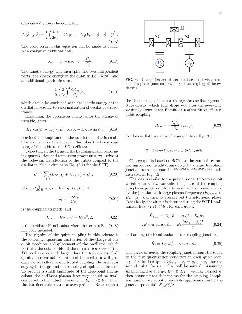
29

difference φ across the oscillator,

K(φ−,i; φ) =1

2

(

h

2e

)2[

2Cφ2−,i + Cg(Vgi − φ− φ−,i)

2]

.

(9.16)The cross term in this equation can be made to vanishby a change of qubit variable,

φ−,i = φi − aφ, a =Cg

CΣ. (9.17)

The kinetic energy will then split into two independentparts, the kinetic energy of the qubit in Eq. (5.28), andan additional quadratic term,

1

2

(

h

2e

)2CCg

CΣφ2, (9.18)

which should be combined with the kinetic energy of theoscillator, leading to renormalization of oscillator capac-itance.

Expanding the Josephson energy, after the change ofvariable, gives

EJi cos(φi − aφ) ≈ EJi cosφi − EJiaφ sinφi . (9.19)

provided the amplitude of the oscillations of φ is small.The last term in this equation describes the linear cou-pling of the qubit to the LC-oscillator.

Collecting all the terms in the Lagrangian and perform-ing quantization and truncation procedures, we arrive atthe following Hamiltonian of the qubits coupled to theoscillator (this is similar to Eq. (8.4) for the SCT),

H =∑

i=1,2

(HSCB,i + λiσyiφ) + Hosc, (9.20)

where H(i)SCB is given by Eq. (7.5), and

λi =EJiCg

CΣ, (9.21)

is the coupling strength, and

Hosc = ECoscn2 + ELφ

2/2, (9.22)

is the oscillator Hamiltonian where the term in Eq. (9.18)has been included.

The physics of the qubit coupling in this scheme isthe following: quantum fluctuation of the charge of onequbit produces a displacement of the oscillator, whichperturbs the other qubit. If the plasma frequency of theLC oscillator is much larger than the frequencies of allqubits, then virtual excitation of the oscillator will pro-duce a direct effective qubit-qubit coupling, the oscillatorstaying in the ground state during all qubit operations.To provide a small amplitude of the zero-point fluctu-ations, the oscillator plasma frequency should be smallcompared to the inductive energy, or ECosc ≪ EL. Thenthe fast fluctuations can be averaged out. Noticing that

Vg

SCT

Vg

SCT

JJ

FIG. 32: Charge (charge-phase) qubits coupled via a com-mon Josephson junction providing phase coupling of the twocircuits

the displacement does not change the oscillator groundstate energy, which then drops out after the averaging,we finally arrive at the Hamiltonian of the direct effectivequbit coupling,

Hint = −λ1λ2

ELσy1σy2. (9.23)

for the oscillator-coupled charge qubits in Fig. 31.

2. Current coupling of SCT qubits

Charge qubits based on SCTs can be coupled by con-necting loops of neighboring qubits by a large Josephsonjunction in the common link155,156,157,158,159,160,161, as il-lustrated in Fig. 32,

The idea is similar to the previous one: to couple qubitvariables to a new variable, the phase of the couplingJosephson junction, then to arrange the phase regimefor the junction with large plasma frequency (ECcoupl ≪EJcoupl), and then to average out the additional phase.Technically, the circuit is described using the SCT Hamil-tonian, Eqs. (7.7), (7.8), for each qubit,

HSCT = EC(n− − ng)2 + EC n

2+

−2EJ cosφ+ cosφ− + EL(2φ+ − φe)

2

2, (9.24)

and adding the Hamiltonian of the coupling junction,

Hc = EC,cn2c − EJ,c cosφc. (9.25)

The phase φc across the coupling junction must be addedto the flux quantization condition in each qubit loop;e.g., for the first qubit 2φ+,1 + φc = φe,1 + φ1 (for thesecond qubit the sign of φc will be minus). Assuming

small inductive energy, EL ≪ EJ,c, we may neglect φ;then assuming the flux regime for the coupling Joseph-son junction we adopt a parabolic approximation for thejunction potential, EJ,cφ

2c/2.

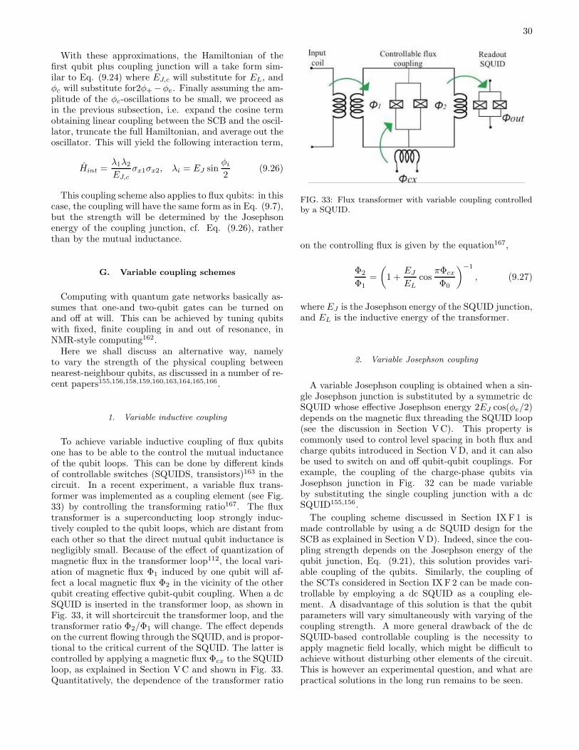
30

With these approximations, the Hamiltonian of thefirst qubit plus coupling junction will a take form sim-ilar to Eq. (9.24) where EJ,c will substitute for EL, andφc will substitute for2φ+ −φe. Finally assuming the am-plitude of the φc-oscillations to be small, we proceed asin the previous subsection, i.e. expand the cosine termobtaining linear coupling between the SCB and the oscil-lator, truncate the full Hamiltonian, and average out theoscillator. This will yield the following interaction term,

Hint =λ1λ2

EJ,cσx1σx2, λi = EJ sin

φi

2(9.26)

This coupling scheme also applies to flux qubits: in thiscase, the coupling will have the same form as in Eq. (9.7),but the strength will be determined by the Josephsonenergy of the coupling junction, cf. Eq. (9.26), ratherthan by the mutual inductance.

G. Variable coupling schemes

Computing with quantum gate networks basically as-sumes that one-and two-qubit gates can be turned onand off at will. This can be achieved by tuning qubitswith fixed, finite coupling in and out of resonance, inNMR-style computing162.

Here we shall discuss an alternative way, namelyto vary the strength of the physical coupling betweennearest-neighbour qubits, as discussed in a number of re-cent papers155,156,158,159,160,163,164,165,166.

1. Variable inductive coupling

To achieve variable inductive coupling of flux qubitsone has to be able to the control the mutual inductanceof the qubit loops. This can be done by different kindsof controllable switches (SQUIDS, transistors)163 in thecircuit. In a recent experiment, a variable flux trans-former was implemented as a coupling element (see Fig.33) by controlling the transforming ratio167. The fluxtransformer is a superconducting loop strongly induc-tively coupled to the qubit loops, which are distant fromeach other so that the direct mutual qubit inductance isnegligibly small. Because of the effect of quantization ofmagnetic flux in the transformer loop112, the local vari-ation of magnetic flux Φ1 induced by one qubit will af-fect a local magnetic flux Φ2 in the vicinity of the otherqubit creating effective qubit-qubit coupling. When a dcSQUID is inserted in the transformer loop, as shown inFig. 33, it will shortcircuit the transformer loop, and thetransformer ratio Φ2/Φ1 will change. The effect dependson the current flowing through the SQUID, and is propor-tional to the critical current of the SQUID. The latter iscontrolled by applying a magnetic flux Φcx to the SQUIDloop, as explained in Section VC and shown in Fig. 33.Quantitatively, the dependence of the transformer ratio

FIG. 33: Flux transformer with variable coupling controlledby a SQUID.

on the controlling flux is given by the equation167,

Φ2

Φ1=

(

1 +EJ

ELcos

πΦcx

Φ0

)−1

, (9.27)

where EJ is the Josephson energy of the SQUID junction,and EL is the inductive energy of the transformer.

2. Variable Josephson coupling

A variable Josephson coupling is obtained when a sin-gle Josephson junction is substituted by a symmetric dcSQUID whose effective Josephson energy 2EJ cos(φe/2)depends on the magnetic flux threading the SQUID loop(see the discussion in Section VC). This property iscommonly used to control level spacing in both flux andcharge qubits introduced in Section VD, and it can alsobe used to switch on and off qubit-qubit couplings. Forexample, the coupling of the charge-phase qubits viaJosephson junction in Fig. 32 can be made variableby substituting the single coupling junction with a dcSQUID155,156.

The coupling scheme discussed in Section IXF1 ismade controllable by using a dc SQUID design for theSCB as explained in Section VD). Indeed, since the cou-pling strength depends on the Josephson energy of thequbit junction, Eq. (9.21), this solution provides vari-able coupling of the qubits. Similarly, the coupling ofthe SCTs considered in Section IX F2 can be made con-trollable by employing a dc SQUID as a coupling ele-ment. A disadvantage of this solution is that the qubitparameters will vary simultaneously with varying of thecoupling strength. A more general drawback of the dcSQUID-based controllable coupling is the necessity toapply magnetic field locally, which might be difficult toachieve without disturbing other elements of the circuit.This is however an experimental question, and what arepractical solutions in the long run remains to be seen.

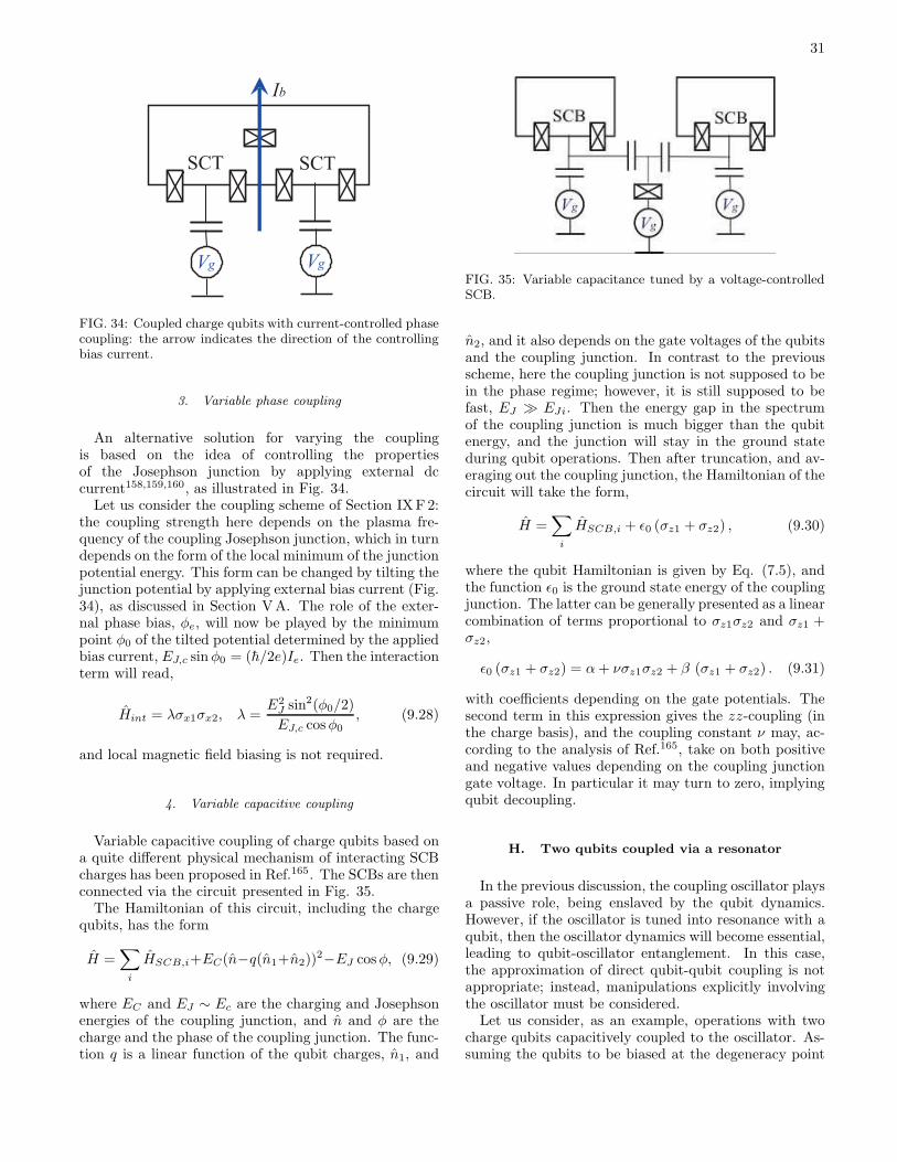
31

Vg

SCT

Vg

SCT

Ib

FIG. 34: Coupled charge qubits with current-controlled phasecoupling: the arrow indicates the direction of the controllingbias current.

3. Variable phase coupling

An alternative solution for varying the couplingis based on the idea of controlling the propertiesof the Josephson junction by applying external dccurrent158,159,160, as illustrated in Fig. 34.

Let us consider the coupling scheme of Section IXF2:the coupling strength here depends on the plasma fre-quency of the coupling Josephson junction, which in turndepends on the form of the local minimum of the junctionpotential energy. This form can be changed by tilting thejunction potential by applying external bias current (Fig.34), as discussed in Section VA. The role of the exter-nal phase bias, φe, will now be played by the minimumpoint φ0 of the tilted potential determined by the appliedbias current, EJ,c sinφ0 = (h/2e)Ie. Then the interactionterm will read,

Hint = λσx1σx2, λ =E2

J sin2(φ0/2)

EJ,c cosφ0, (9.28)

and local magnetic field biasing is not required.

4. Variable capacitive coupling

Variable capacitive coupling of charge qubits based ona quite different physical mechanism of interacting SCBcharges has been proposed in Ref.165. The SCBs are thenconnected via the circuit presented in Fig. 35.

The Hamiltonian of this circuit, including the chargequbits, has the form

H =∑

i

HSCB,i+EC(n−q(n1+n2))2−EJ cosφ, (9.29)

where EC and EJ ∼ Ec are the charging and Josephsonenergies of the coupling junction, and n and φ are thecharge and the phase of the coupling junction. The func-tion q is a linear function of the qubit charges, n1, and

FIG. 35: Variable capacitance tuned by a voltage-controlledSCB.

n2, and it also depends on the gate voltages of the qubitsand the coupling junction. In contrast to the previousscheme, here the coupling junction is not supposed to bein the phase regime; however, it is still supposed to befast, EJ ≫ EJi. Then the energy gap in the spectrumof the coupling junction is much bigger than the qubitenergy, and the junction will stay in the ground stateduring qubit operations. Then after truncation, and av-eraging out the coupling junction, the Hamiltonian of thecircuit will take the form,

H =∑

i

HSCB,i + ǫ0 (σz1 + σz2) , (9.30)

where the qubit Hamiltonian is given by Eq. (7.5), andthe function ǫ0 is the ground state energy of the couplingjunction. The latter can be generally presented as a linearcombination of terms proportional to σz1σz2 and σz1 +σz2,

ǫ0 (σz1 + σz2) = α+ νσz1σz2 + β (σz1 + σz2) . (9.31)

with coefficients depending on the gate potentials. Thesecond term in this expression gives the zz-coupling (inthe charge basis), and the coupling constant ν may, ac-cording to the analysis of Ref.165, take on both positiveand negative values depending on the coupling junctiongate voltage. In particular it may turn to zero, implyingqubit decoupling.

H. Two qubits coupled via a resonator

In the previous discussion, the coupling oscillator playsa passive role, being enslaved by the qubit dynamics.However, if the oscillator is tuned into resonance with aqubit, then the oscillator dynamics will become essential,leading to qubit-oscillator entanglement. In this case,the approximation of direct qubit-qubit coupling is notappropriate; instead, manipulations explicitly involvingthe oscillator must be considered.

Let us consider, as an example, operations with twocharge qubits capacitively coupled to the oscillator. As-suming the qubits to be biased at the degeneracy point

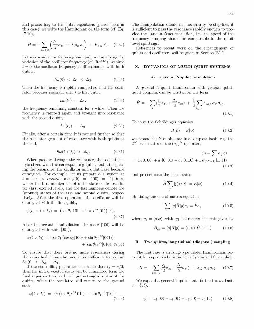
32

and proceeding to the qubit eigenbasis (phase basis inthis case), we write the Hamiltonian on the form (cf. Eq.(7.10),

H = −∑

i=1,2

(

∆i

2σzi − λiσx φi

)

+ Hosc[φ]. (9.32)

Let us consider the following manipulation involving thevariation of the oscillator frequency (cf. Ref164): at timet = 0, the oscillator frequency is off-resonance with bothqubits,

hω(0) < ∆1 < ∆2. (9.33)

Then the frequency is rapidly ramped so that the oscil-lator becomes resonant with the first qubit,

hω(t1) = ∆1, (9.34)

the frequency remaining constant for a while. Then thefrequency is ramped again and brought into resonancewith the second qubit,

hω(t2) = ∆2. (9.35)

Finally, after a certain time it is ramped further so thatthe oscillator gets out of resonance with both qubits atthe end,

hω(t > t3) > ∆2. (9.36)

When passing through the resonance, the oscillator ishybridized with the corresponding qubit, and after pass-ing the resonance, the oscillator and qubit have becomeentangled. For example, let us prepare our system att = 0 in the excited state ψ(0) = |100〉 = |1〉|0〉|0〉,where the first number denotes the state of the oscilla-tor (first excited level), and the last numbers denote the(ground) states of the first and second qubits, respec-tively. After the first operation, the oscillator will beentangled with the first qubit,

ψ(t1 < t < t2) =(

cos θ1|10〉 + sin θ1eiα|01〉

)

|0〉.(9.37)

After the second manipulation, the state |100〉 will beentangled with state |001〉,

ψ(t > t3) = cos θ1(

cos θ2|100〉+ sin θ2eiβ |001〉

)

+ sin θ1eiα|010〉. (9.38)

To ensure that there are no more resonances duringthe described manipulations, it is sufficient to requirehω(0) > ∆2 − ∆1.

If the controlling pulses are chosen so that θ2 = π/2,then the initial excited state will be eliminated form thefinal superposition, and we’ll get entangled states of thequbits, while the oscillator will return to the groundstate,

ψ(t > t3) = |0〉(

cos θ1eiβ |01〉) + sin θ1e

iα|10〉)

.(9.39)

The manipulation should not necessarily be step-like, itis sufficient to pass the resonance rapidly enough to pro-vide the Landau-Zener transition, i.e. the speed of thefrequency ramping should be comparable to the qubitlevel splittings.

References to recent work on the entanglement ofqubits and oscillators will be given in Section IV C.

X. DYNAMICS OF MULTI-QUBIT SYSTEMS

A. General N-qubit formulation

A general N-qubit Hamiltonian with general qubit-qubit coupling can be written on the form

H = −∑

i

(ǫi2σzi +

∆i

2σxi) +

1

2

∑

i,j;ν

λν,ij σνiσνj

(10.1)

To solve the Schrodinger equation

H |ψ〉 = E|ψ〉 (10.2)

we expand the N-qubit state in a complete basis, e.g. the2N basis states of the (σz)

N operator,

|ψ〉 =∑

aq|q〉= a0|0..00〉 + a1|0..01〉 + a2|0..10〉 + ...a(2N−1)|1..11〉

(10.3)

and project onto the basis states

H∑

p

|p〉〈p|ψ〉 = E|ψ〉 (10.4)

obtaining the ususal matrix equation

∑

p

〈q|H |p〉ap = Eaq (10.5)

where aq = 〈q|ψ〉, with typical matrix elements given by

Hqp = 〈q|H |p〉 = 〈1..01|H |0..11〉 (10.6)

B. Two qubits, longitudinal (diagonal) coupling

The first case is an Ising-type model Hamiltonian, rel-evant for capacitively or inductively coupled flux qubits,

H = −∑

i=1,2

(ǫi2σzi +

∆i

2σxi) + λ12 σz1σz2 (10.7)

We expand a general 2-qubit state in the the σz basisq = kl,

|ψ〉 = a1|00〉 + a2|01〉 + a3|10〉 + a4|11〉 (10.8)

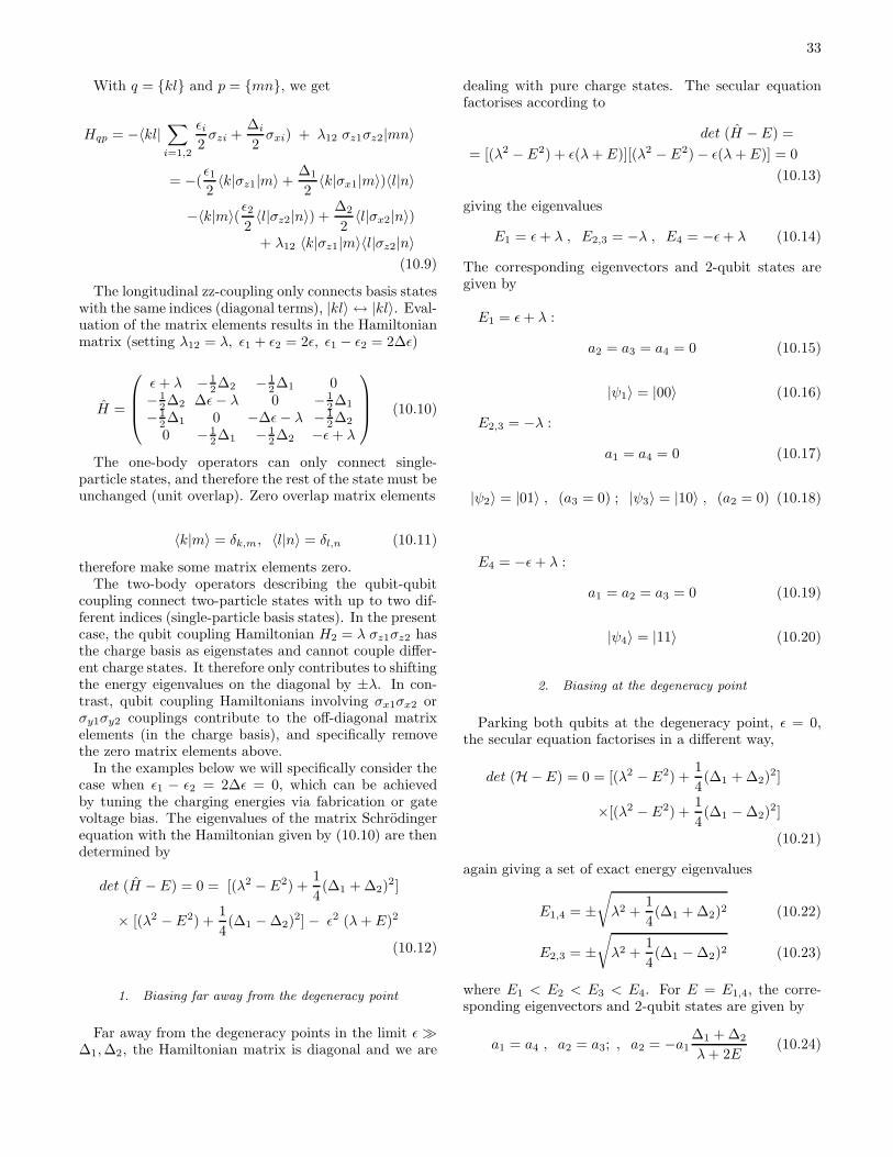
33

With q = kl and p = mn, we get

Hqp = −〈kl|∑

i=1,2

ǫi2σzi +

∆i

2σxi) + λ12 σz1σz2|mn〉

= −(ǫ12〈k|σz1|m〉 +

∆1

2〈k|σx1|m〉)〈l|n〉

−〈k|m〉(ǫ22〈l|σz2|n〉) +

∆2

2〈l|σx2|n〉)

+ λ12 〈k|σz1|m〉〈l|σz2|n〉(10.9)

The longitudinal zz-coupling only connects basis stateswith the same indices (diagonal terms), |kl〉 ↔ |kl〉. Eval-uation of the matrix elements results in the Hamiltonianmatrix (setting λ12 = λ, ǫ1 + ǫ2 = 2ǫ, ǫ1 − ǫ2 = 2∆ǫ)

H =

ǫ+ λ − 12∆2 − 1

2∆1 0− 1

2∆2 ∆ǫ− λ 0 − 12∆1

− 12∆1 0 −∆ǫ− λ − 1

2∆2

0 − 12∆1 − 1

2∆2 −ǫ+ λ

(10.10)

The one-body operators can only connect single-particle states, and therefore the rest of the state must beunchanged (unit overlap). Zero overlap matrix elements

〈k|m〉 = δk,m, 〈l|n〉 = δl,n (10.11)

therefore make some matrix elements zero.The two-body operators describing the qubit-qubit

coupling connect two-particle states with up to two dif-ferent indices (single-particle basis states). In the presentcase, the qubit coupling Hamiltonian H2 = λ σz1σz2 hasthe charge basis as eigenstates and cannot couple differ-ent charge states. It therefore only contributes to shiftingthe energy eigenvalues on the diagonal by ±λ. In con-trast, qubit coupling Hamiltonians involving σx1σx2 orσy1σy2 couplings contribute to the off-diagonal matrixelements (in the charge basis), and specifically removethe zero matrix elements above.

In the examples below we will specifically consider thecase when ǫ1 − ǫ2 = 2∆ǫ = 0, which can be achievedby tuning the charging energies via fabrication or gatevoltage bias. The eigenvalues of the matrix Schrodingerequation with the Hamiltonian given by (10.10) are thendetermined by

det (H − E) = 0 = [(λ2 − E2) +1

4(∆1 + ∆2)

2]

× [(λ2 − E2) +1

4(∆1 − ∆2)

2] − ǫ2 (λ+ E)2

(10.12)

1. Biasing far away from the degeneracy point

Far away from the degeneracy points in the limit ǫ ≫∆1,∆2, the Hamiltonian matrix is diagonal and we are

dealing with pure charge states. The secular equationfactorises according to

det (H − E) =

= [(λ2 − E2) + ǫ(λ+ E)][(λ2 − E2) − ǫ(λ+ E)] = 0

(10.13)

giving the eigenvalues

E1 = ǫ+ λ , E2,3 = −λ , E4 = −ǫ+ λ (10.14)

The corresponding eigenvectors and 2-qubit states aregiven by

E1 = ǫ+ λ :

a2 = a3 = a4 = 0 (10.15)

|ψ1〉 = |00〉 (10.16)

E2,3 = −λ :

a1 = a4 = 0 (10.17)

|ψ2〉 = |01〉 , (a3 = 0) ; |ψ3〉 = |10〉 , (a2 = 0) (10.18)

E4 = −ǫ+ λ :

a1 = a2 = a3 = 0 (10.19)

|ψ4〉 = |11〉 (10.20)

2. Biasing at the degeneracy point

Parking both qubits at the degeneracy point, ǫ = 0,the secular equation factorises in a different way,

det (H−E) = 0 = [(λ2 − E2) +1

4(∆1 + ∆2)

2]

×[(λ2 − E2) +1

4(∆1 − ∆2)

2]

(10.21)

again giving a set of exact energy eigenvalues

E1,4 = ±√

λ2 +1

4(∆1 + ∆2)2 (10.22)

E2,3 = ±√

λ2 +1

4(∆1 − ∆2)2 (10.23)

where E1 < E2 < E3 < E4. For E = E1,4, the corre-sponding eigenvectors and 2-qubit states are given by

a1 = a4 , a2 = a3; , a2 = −a1∆1 + ∆2

λ+ 2E(10.24)

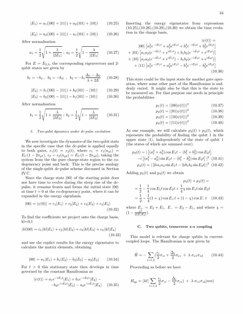
34

|E1〉 = a1(|00〉 + |11〉) + a2(|01〉 + |10〉) (10.25)

|E4〉 = a2(|00〉 + |11〉) − a1(|01〉 + |10〉) (10.26)

After normalisation

a1 =1

2

√

1 +λ

|2E1|; a2 =

1

2

√

1 − λ

|2E1|(10.27)

For E = E2,3, the corresponding eigenvectors and 2-qubit states are given by

b1 = −b4 , b2 = −b3; , b2 = −b1∆1 − ∆2

λ+ 2E(10.28)

|E2〉 = b1(|00〉 − |11〉) + b2(|01〉 − |10〉) (10.29)

|E3〉 = b2(|00〉 − |11〉) − b1(|01〉 − |10〉) (10.30)

After normalisation

b1 =1

2

√

1 +λ

|2E2|; b2 =

1

2

√

1 − λ

|2E2|(10.31)

3. Two-qubit dynamics under dc-pulse excitation

We now investigate the dynamics of the two-qubit statein the specific case that the dc-pulse is applied equallyto both gates, ǫ1(t) = ǫ2(t), where ǫ1 = ǫ1(ng1) =EC(1 − 2ng1), ǫ2 = ǫ2(ng2) = EC(1 − 2ng2), taking thesystem from the the pure charge-state region to the co-degeneracy point and back. This is the precise analogyof the single-qubit dc-pulse scheme discussed in SectionIVC.

Since the charge state |00〉 of the starting point doesnot have time to evolve during the steep rise of the dc-pulse, it remains frozen and forms the initial state |00〉at time t = 0 at the co-degeneracy point, where it can beexpanded in the energy eigenbasis,

|00〉 = |ψ(0)〉 = c1|E1〉 + c2|E2〉 + c3|E3〉 + c4|E4〉(10.32)

To find the coefficients we project onto the charge basis,kl=0,1

〈kl|00〉 = c1〈kl|E1〉 + c2〈kl|E2〉 + c3〈kl|E3〉 + c4〈kl|E4〉(10.33)

and use the explict results for the energy eigenstates tocalculate the matrix elements, obtaining

|00〉 = a1|E1〉 + b1|E2〉 − b2|E3〉 − a2|E4〉 (10.34)

For t > 0 this stationary state then develops in timegoverned by the constant Hamiltonian as

|ψ(t)〉 = a1e−iE1t|E1〉 + b1e

−iE2t|E2〉 −−b2e+iE2t|E3〉 − a2e

+iE1t|E4〉 (10.35)

Inserting the energy eigenstates from expressions(10.25),(10.26),(10.29),(10.30) we obtain the time evolu-tion in the charge basis,

|ψ(t)〉 =

|00〉[

a21e

−iE1t + a22e

iE1t + b21e−iE2t + b22e

iE2t]

+ |01〉[

a1a2(e−iE1t + eiE1t) + b1b2(e

−iE2t + eiE2t)]

+ |10〉[

a1a2(e−iE1t + eiE1t) − b1b2(e

−iE2t + eiE2t)]

+ |11〉[

a21e

−iE1t + a22e

iE1t − b21e−iE2t − b22e

iE2t]

(10.36)

This state could be the input state for another gate oper-ation, where some other part of the Hamiltonian is sud-denly varied. It might also be that this is the state tobe measured on. For that purpose one needs in principlethe probabilities

p1(t) = |〈00|ψ(t)〉|2 (10.37)

p2(t) = |〈01|ψ(t)〉|2 (10.38)

p3(t) = |〈10|ψ(t)〉|2 (10.39)

p4(t) = |〈11|ψ(t)〉|2 (10.40)

As one example, we will calculate p3(t) + p4(t), whichrepresents the probability of finding the qubit 1 in theupper state |1〉, independently of the state of qubit 1(the states of which are summed over).

p3(t) = |[

(a21 + a2

2) cosE1t− (b21 + b22) cosE2t]

−i[

(a21 − a2

2) sinE1t− (b21 − b22) sinE2t]

|2 (10.41)

p4(t) = | [2ia1a2 sinE1t− 2ib1b2 sinE2t] |2 (10.42)

Adding p3(t) and p4(t) we obtain

p3(t) + p4(t) =

=1

2− 1

4cosE1t cosE2t+

1

4χ sinE1t sinE2t

=1

2− 1

4(1 + χ) cosE+t+ (1 − χ) cosE−t (10.43)

where E+ = E2 + E1, E− = E2 − E1, and where χ =

(1 − λ2

2|E1E2| ).

C. Two qubits, transverse x-x coupling

This model is relevant for charge qubits in current-coupled loops. The Hamiltonian is now given by

H = −∑

i=1,2

(ǫi2σzi +

∆i

2σxi + λ σx1σx2 (10.44)

Proceeding as before we have

Hqp = 〈kl|∑

i=1,2

ǫi2σzi −

∆i

2σxi) + λ σz1σz2|mn〉

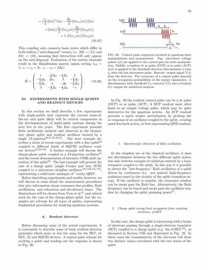
35

= (ǫ12〈k|σ(1)

z |m〉 − ∆1

2〈k|σx1|m〉)〈l|n〉

+〈k|m〉(ǫ22〈l|σz2|n〉)

∆2

2〈l|σx2|n〉)

+ λ 〈k|σx1|m〉〈l|σx2|n〉(10.45)

This coupling only connects basis states which differ inboth indices (”anti-diagonal” terms), i.e. |00〉 ↔ |11〉 and|01〉 ↔ |10〉, meaning that interaction will only appearon the anti-diagonal. Evaluation of the matrix elementsresult in the Hamiltonian matrix (again setting λ12 =λ, ǫ1 + ǫ2 = 2ǫ, ǫ1 − ǫ2 = 2∆ǫ)

H =

ǫ − 12∆2 − 1

2∆1 λ− 1

2∆2 ∆ǫ1 λ − 12∆1

− 12∆1 λ −∆ǫ − 1

2∆2

λ − 12∆1 − 1

2∆2 −ǫ

, (10.46)

XI. EXPERIMENTS WITH SINGLE QUBITSAND READOUT DEVICES

In this section we shall describe a few experimentswith single-qubits that represent the current state-of-the-art and quite likely will be central components inthe developmement of multi-qubit systems during thenext five to ten years. The first experiment presentsRabi oscillations induced and observed in the elemen-tary phase qubit and readout oscillator formed by asingle JJ-junction30,31,32,33,34. The next example de-scribes a series of recent experiments with a flux qubit24

coupled to different kinds of SQUID oscillator read-out devices25,26,168. A further example will discuss thecharge-phase qubit coupled to a JJ-junction oscillator21

and the recent demonstration of extensive NMR-style op-eration of this qubit23. The last example will present thecase of a charge qubit (single Cooper pair box, SCB)coupled to a microwave stripline oscillator147,148,151,152,representing a solid-state analogue of ”cavity QED”.

Before describing experiments and results, however, wewill discuss in some detail the measurement proceduresthat give information about resonance line profiles, Rabioscillations, and relaxation and decohrence times. Theillustrations will be chosen from Vion et al.21 and relatedwork for the case of the charge-phase qubit, but the ex-amples are relevant for all types of qubits, representingfundmental procedures for studying quantum systems.

A. Readout detectors

Before discussing some of the actual experiments, itis convenient to describe some of basic readout-detectorprinciples which more or less the same for the SET, rf-SET, JJ and SQUID devices. A typical pulse scheme forexciting a qubit and reading out the response is shownin Fig. 36:

FIG. 36: Control pulse sequences involved in quantum statemanipulations and measurement. Top: microwave voltagepulses u(t) are applied to the control gate for state manipula-tion. Middle: a readout dc ac pulse (DCP) or ac pulse (ACP)Ib(t) is applied to the threshold detector/discriminator a timetd after the last microwave pulse. Bottom: output signal V(t)from the detector. The occurence of a output pulse dependson the occupation probabilities of the energy eigenstates. Adiscriminator with threshold Vth converts V(t) into a boolean0/1 output for statistical analysis.

In Fig. 36 the readout control pulse can be a dc pulse(DCP) or ac pulse (ACP). A DCP readout most oftenleads to an output voltage pulse, which may be quitedestructive for the quantum system. An ACP readoutpresents a much weaker perturbation by probing theac-response of an oscillator coupled to the qubit, creatingmuch less back action, at best representing QND readout.

1. Spectroscopic detection of Rabi oscillation

In the simplest use of the classical oscillator, it doesnot discriminate between the two different qubit states,but only between energies of radiation emitted by a lossyresonator coupled to the qubit. In this way it is possibleto detect the ”low-frequency” Rabi oscillation of a qubitdriven by continuous (i.e. not pulsed) high-frequencyradiation tuned in the vicinity of the qubit transition en-ergy. If the oscillator is tunable, the resonance windowcan be swept past the Rabi line. Alternatively, the Rabifrequency can be tuned and swept past the oscillator win-dow by changing the qubit pumping power27.

2. Charge qubit energy level occupation from countingelectrons: rf-SET

In this case, the charge qubit is interacting with a beamof electrons passing through a single-electron transistor(SET) coupled to a charge qubit (e.g. the rf-SET,69), asdiscussed in Section VIII and illustrated in Fig. 22. Inthese cases the transmissivity of the electrons will showtwo distinct values correlated with the two states of thequbit.

36

Ic

2∆ eV

I

FIG. 37: Current-voltage characteristic of tunnel junction(solid line) consists of the Josephson branch - vertical line atV = 0, and the dissipative branch - curve at eV ≥ 2∆. Whenthe current is ramped, the junction stays at the Josephsonbranch and when the current approaches the critical value Ic,the junction switches to the dissipative branch (dashed line).

3. Coupled qubit-classical-oscillator system: switchingdetectors with dc-pulse (DCP) output

In Section VIII we analyzed the case of an SCT qubitcurrent-coupled to a JJ-oscillator (Fig. 25) and discussedthe Hamiltonian of the coupled qubit-JJ-oscillator sys-tem. The effect of the qubit was to deform the oscillatorpotential in different ways depending on the state of thequbit. The effect can then be probed in a number ofways, by input and output dc and ac voltage and currentpulses, to determine the occupation of the qubit energylevels.

Using non-linear oscillators like single JJs or SQUIDSone can achieve threshold and switching behaviour wherethe JJ/SQUID switches out of the zero-voltage state, re-sulting in an output dc-voltage pulse.

Switching JJ: The method is based on the dependenceof the critical current of the JJ on the state of the qubit,and consists of applying a short current DCP to the JJat a value Ib during a time ∆t, so that the JJ will switchout of its zero-voltage state with a probability Psw(Ib).For well-chosen parameters, the detection efficiency canapproach unity. The switching probability then directlymeasures the qubit’s energy level population.

Switching SQUID: In the experiments on flux qubitsby the Delft group, two kinds of physical coupling ofthe SQUID to the qubit have been implemented, namelyinductive coupling (Fig. 38 (left))7,168 and direct cou-pling (Fig. 38 (right)):24,25,26 The critical current ofthe SQUID depends on the flux threading the loop, andtherefore is different for different qubit states. The prob-lem is to detect a two percent variation in the SQUIDcritical current associated with a transition between thequbit states in a time shorter than the qubit energy relax-ation time T1. The SQUID behaves as an oscillator with acharacteristic plasma frequency ωp = [(L+LJ)Csh]−1/2.This frequency depends on the bias current Ib and onthe critical current IC via the Josephson inductanceLJ = Φ0/2πIC

√

1 − I2b /I

2c (the shunt capacitor with ca-

FIG. 38: Schematics of readout dc SQUID coupled to fluxqubit; left - inductive coupling, right - direct phase coupling

pacitance Csh and lead inductance L is used to ”tune”ωp). Thus, the plasma frequency takes different values

ω(0)p or ω

(1)p depending on the state of qubit, representing

two different shapes of the SQUID oscillator potential.

In the dc-pulse-triggered switching SQUID7,24,25, adc-current readout-pulse is applied after the operationpulse(s) (Fig. 36), setting a switching threshold for thecritical current. The circulating qubit current for onequbit state will then add to the critical current and makethe SQUID switch to the voltage state, while the otherqubit state will reduce the current and leave the SQUIDin the zero-voltage state.

In an application of ac-pulse-triggered switchingSQUID26, readout relies on resonant activation by a mi-crowave pulse at a frequency close to ωp, adjusting thepower so that the SQUID switches to the finite voltagestate by resonant activation if the qubit is in state |0〉,whereas it stays in the zero-voltage state if it is in state|1〉. The resonant activation scheme is similar to the read-out scheme used by Martinis et al.30,31,32,33. (see SectionXI C).

4. Coupled qubit-classical-oscillator system: ac-pulse(ACP) non-switching detectors

This implementation of ACP readout uses the qubit-SQUID combination7 shown in Fig. 38 (left), but withACP instead of DCP readout, implementing a nonde-structive dispersive method for the readout of the fluxqubit168. The detection is based on the measurementof the Josephson inductance of a dc-SQUID inductivelycoupled to the qubit. Using this method, Lupascu etal.168 measured the spectrum of the qubit resonance lineand obtained relaxation times around 80 µs, much longerthan observed with DCP.

A related readout scheme was recently implemented bySiddiqi et al.169 using two different oscillation states ofthe non-linear JJ in the zero-voltage state.

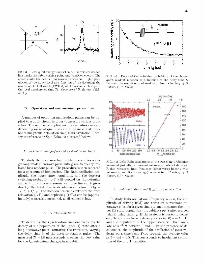
37

FIG. 39: Left: qubit energy level scheme. The vertical dashedline marks the qubit working point and transition energy. Thearrow marks the detuned microwave excitation. Right: pop-ulation of the upper level as a function of the detuning; theinverse of the half width (FWHM) of the resonance line givesthe total decoherence time T2. Courtesy of D. Esteve, CEA-Saclay.

.

B. Operation and measurement procedures

A number of operation and readout pulses can be ap-plied to a qubit circuit in order to measure various prop-erties. The number of applied microwave pulses can varydepending on what quantities are to be measured: reso-nance line profile, relaxation time, Rabi oscillation, Ram-sey interference or Spin Echo, as discussed below.

1. Resonance line profiles and T2 decoherence times

To study the resonance line profile, one applies a sin-gle long weak microwave pulse with given frequency, fol-lowed by a readout pulse. The procedure is then repeatedfor a spectrum of frequencies. The Rabi oscillation am-plitude, the upper state population, and the detectorswitching probability p(t) will depend on the detuningand will grow towards resonance. The linewidth givesdirectly the total inverse decoherence lifetime 1/T2 =1/2T1 + 1/Tφ. The decoherence-time contributions fromrelaxation (1/T1) and dephasing (1/Tφ) can be (approx-imately) separately measured, as discussed below.

2. T1 relaxation times

To determine the T1 relaxation time one measures thedecacy of the population of the upper |1〉 state after along microwave pulse saturating the transition, varyingthe delay time td of the detector readout pulse. Themeasured T1 =1.8 microseconds is so far the best valuefor the Quantronium charge-phase qubit.

FIG. 40: Decay of the switching probability of the charge-qubit readout junction as a function of the delay time tdbetween the excitation and readout pulses. Courtesy of D.Esteve, CEA-Saclay.

FIG. 41: Left: Rabi oscillations of the switching probabilitymeasured just after a resonant microwave pulse of duration.Right: Measured Rabi frequency (dots) varies linearly withmicrowave amplitude (voltage) as expected. Courtesy of D.Esteve, CEA-Saclay.

3. Rabi oscillations and T2,Rabi decoherence time

To study Rabi oscillations (frequency Ω ∼ u, the am-plitude of driving field) one turns on a resonant mi-crowave pulse for a given time tµw and measures the up-per |1〉 state population (probability) p1(t) after a given(short) delay time td. If the systems is perfectly coher-ent, the state vector will develop as cosΩt |0〉+sinΩt |1〉,and the population of the upper state will then oscil-late as sin2 Ωt between 0 and 1. In the presence of de-coherence, the amplitude of the oscillation of p1(t) willdecay on a time scale TRabi towards the average valuep1(t = ∞) = 0.5. This corresponds to incoherent satura-tion of the 0 to 1 transition.

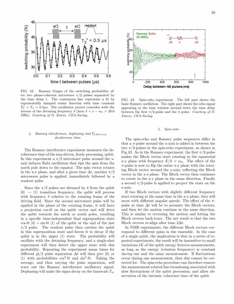
38

FIG. 42: Ramsey fringes of the switching probability af-ter two phase-coherent microwave π/2 pulses separated bythe time delay t. The continuous line represents a fit byexponentially damped cosine function with time constantT ∗

2 = Tφ = 0.5µs. The oscillation period coincides with theinverse of the detuning frequency δ (here δ = ν − ν01 = 20.6MHz). Courtesy of D. Esteve, CEA-Saclay.

4. Ramsey interference, dephasing and T2,Ramsey

decoherence time

The Ramsey interference experiment measures the de-coherence time of the non-driven, freely precessing, qubit.In this experiment a π/2 microwave pulse around the x-axis induces Rabi oscillation that tips the spin from thenorth pole down to the equator. The spin vector rotatesin the x-y plane, and after a given time ∆t, another π/2microwave pulse is applied, immediately followed by areadout pulse.

Since the π/2 pulses are detuned by δ from the qubit|0〉 → |1〉 transition frequency, the qubit will precesswith frequency δ relative to the rotating frame of thedriving field. Since the second microwave pulse will beapplied in the plane of the rotating frame, it will havea projection cos δt on the qubit vector and will drivethe qubit towards the north or south poles, resultingin a specific time-independent final superposition statecos δt |0〉 + sin δt |1〉 of the qubit at the end of the lastπ/2 pulse. The readout pulse then catches the qubitin this superposition state and forces it to decay if thequbit is in the upper |1〉 state. The probability willoscillate with the detuning frequency, and a single-shotexperiment will then detect the upper state with thisprobability. Repeating the experiment many times fordifferent pi/2 pulse separation ∆t will then give |0〉 or|1〉 with probabilities cos2 δt and sin2 δt. Taking theaverage, and then varying the pulse separation, willtrace out the Ramsey interference oscillatory signal.Dephasing will make the signa decay on the timescale Tφ.

FIG. 43: Spin-echo experiment. The left part shows thebasic Ramsey oscillation. The right part shows the echo signalappearing in the time window around twice the time delaybetween the first π/2-pulse and the π-pulse. Courtesy of D.Esteve, CEA-Saclay.

5. Spin-echo

The spin-echo and Ramsey pulse sequences differ inthat a π-pulse around the x-axis is added in between thetwo π/2-pulses in the spin-echo experiment, as shown inFig.43. As in the Ramsey experiment, the first π/2-pulsemakes the Bloch vector start rotating in the equatorialx-y plane with frequency E/h = ν01. The effect of theπ-pulse is now to flip the entire x-y plane with the rotat-ing Bloch vector around the x-axis, reflecting the Blochvector in the x-z plane. The Bloch vector then continuesto rotate in the x-y plane in the same direction. Finallya second π/2-pulse is applied to project the state on thez-axis.

If two Bloch vectors with slightly different frequencystart rotating at the same time in the x-y plane, they willmove with different angular speeds. The effect of the π-pulse at time ∆t will be to permute the Bloch vectors,and then let the motion continue in the same direction.This is similar to reversing the motion and letting theBloch vectors back-trace. The net result is that the twoBloch vectors re-align after time 2∆t.

In NMR experiments, the different Bloch vectors cor-respond to different spins in the ensemble. In the caseof a single qubit, the implication is that in a series of re-peated experiments, the result will be insensitive to smallvariations δE of the qubit energy between measurements,as long as the energy (rotation frequency) is constantduring one and the same measurement. If fluctuationsoccur during one measurement, then this cannot be cor-rected for. The spin-echo procedure can therefore removethe measurement-related line-broadening associated withslow fluctuations of the qubit precession, and allow ob-servation of the intrinsic coherence time of the qubit.

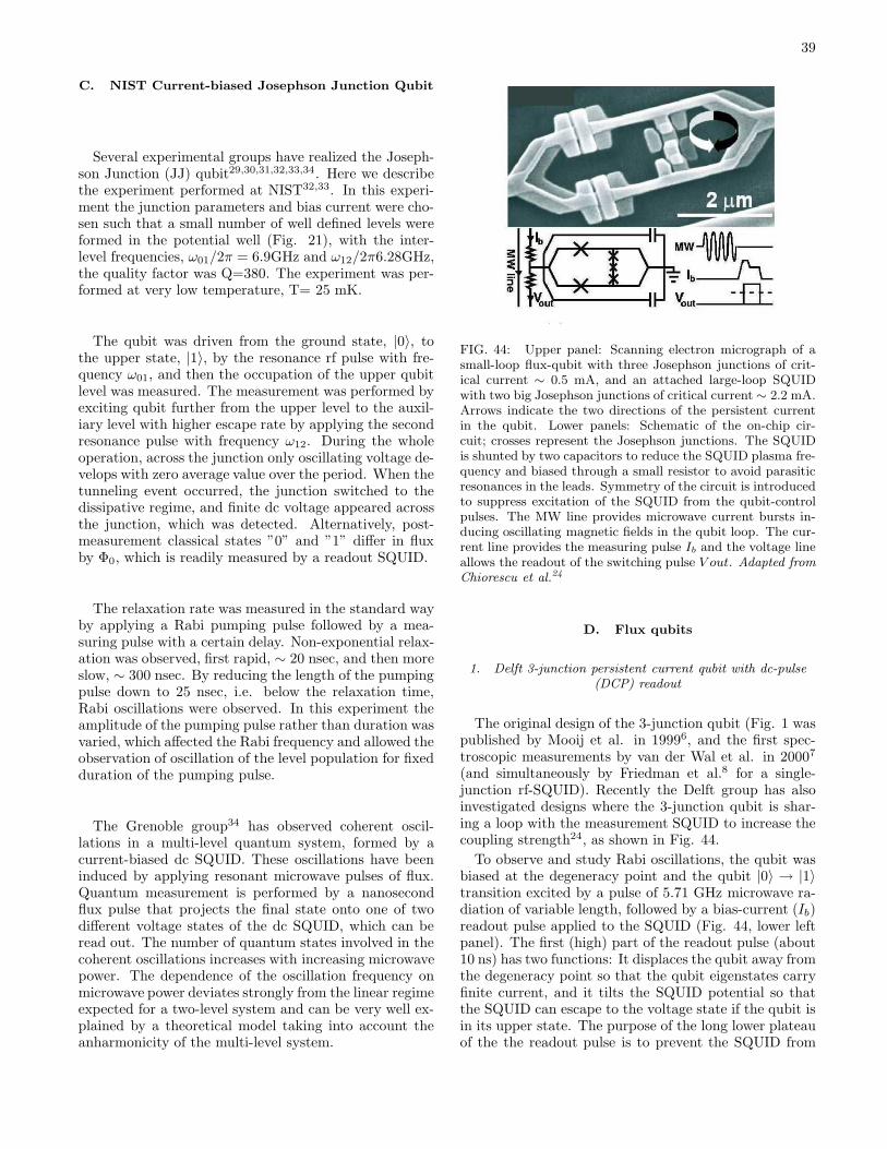
39

C. NIST Current-biased Josephson Junction Qubit

Several experimental groups have realized the Joseph-son Junction (JJ) qubit29,30,31,32,33,34. Here we describethe experiment performed at NIST32,33. In this experi-ment the junction parameters and bias current were cho-sen such that a small number of well defined levels wereformed in the potential well (Fig. 21), with the inter-level frequencies, ω01/2π = 6.9GHz and ω12/2π6.28GHz,the quality factor was Q=380. The experiment was per-formed at very low temperature, T= 25 mK.

The qubit was driven from the ground state, |0〉, tothe upper state, |1〉, by the resonance rf pulse with fre-quency ω01, and then the occupation of the upper qubitlevel was measured. The measurement was performed byexciting qubit further from the upper level to the auxil-iary level with higher escape rate by applying the secondresonance pulse with frequency ω12. During the wholeoperation, across the junction only oscillating voltage de-velops with zero average value over the period. When thetunneling event occurred, the junction switched to thedissipative regime, and finite dc voltage appeared acrossthe junction, which was detected. Alternatively, post-measurement classical states ”0” and ”1” differ in fluxby Φ0, which is readily measured by a readout SQUID.

The relaxation rate was measured in the standard wayby applying a Rabi pumping pulse followed by a mea-suring pulse with a certain delay. Non-exponential relax-ation was observed, first rapid, ∼ 20 nsec, and then moreslow, ∼ 300 nsec. By reducing the length of the pumpingpulse down to 25 nsec, i.e. below the relaxation time,Rabi oscillations were observed. In this experiment theamplitude of the pumping pulse rather than duration wasvaried, which affected the Rabi frequency and allowed theobservation of oscillation of the level population for fixedduration of the pumping pulse.

The Grenoble group34 has observed coherent oscil-lations in a multi-level quantum system, formed by acurrent-biased dc SQUID. These oscillations have beeninduced by applying resonant microwave pulses of flux.Quantum measurement is performed by a nanosecondflux pulse that projects the final state onto one of twodifferent voltage states of the dc SQUID, which can beread out. The number of quantum states involved in thecoherent oscillations increases with increasing microwavepower. The dependence of the oscillation frequency onmicrowave power deviates strongly from the linear regimeexpected for a two-level system and can be very well ex-plained by a theoretical model taking into account theanharmonicity of the multi-level system.

FIG. 44: Upper panel: Scanning electron micrograph of asmall-loop flux-qubit with three Josephson junctions of crit-ical current ∼ 0.5 mA, and an attached large-loop SQUIDwith two big Josephson junctions of critical current ∼ 2.2 mA.Arrows indicate the two directions of the persistent currentin the qubit. Lower panels: Schematic of the on-chip cir-cuit; crosses represent the Josephson junctions. The SQUIDis shunted by two capacitors to reduce the SQUID plasma fre-quency and biased through a small resistor to avoid parasiticresonances in the leads. Symmetry of the circuit is introducedto suppress excitation of the SQUID from the qubit-controlpulses. The MW line provides microwave current bursts in-ducing oscillating magnetic fields in the qubit loop. The cur-rent line provides the measuring pulse Ib and the voltage lineallows the readout of the switching pulse V out. Adapted fromChiorescu et al.24

D. Flux qubits

1. Delft 3-junction persistent current qubit with dc-pulse(DCP) readout

The original design of the 3-junction qubit (Fig. 1 waspublished by Mooij et al. in 19996, and the first spec-troscopic measurements by van der Wal et al. in 20007

(and simultaneously by Friedman et al.8 for a single-junction rf-SQUID). Recently the Delft group has alsoinvestigated designs where the 3-junction qubit is shar-ing a loop with the measurement SQUID to increase thecoupling strength24, as shown in Fig. 44.

To observe and study Rabi oscillations, the qubit wasbiased at the degeneracy point and the qubit |0〉 → |1〉transition excited by a pulse of 5.71 GHz microwave ra-diation of variable length, followed by a bias-current (Ib)readout pulse applied to the SQUID (Fig. 44, lower leftpanel). The first (high) part of the readout pulse (about10 ns) has two functions: It displaces the qubit away fromthe degeneracy point so that the qubit eigenstates carryfinite current, and it tilts the SQUID potential so thatthe SQUID can escape to the voltage state if the qubit isin its upper state. The purpose of the long lower plateauof the the readout pulse is to prevent the SQUID from

40

FIG. 45: AFM picture of the charge-phase qubit (”quantro-nium”) corresponding to the circuit scheme in Fig. 25. Theworking point is controlled by two external ”knobs”, a voltagegate controlling the induced charge (ng) on the SCT island,and a current gate controlling the total phase across the SCTvia the external flux (φe) threading the loop. The large read-out JJ is seen in the left part of the figure. Courtesy of D.Esteve, CEA-Saclay.

returning (”retrapping”) to the zero-voltage state. Withthese operation and readout techniques, Rabi (driven)oscillations, Ramsey (free) oscillations and spin-echos ofthe qubit were observed24, giving a Ramsey free oscil-lation dephasing time of 20 ns and spin echo dephasingtime of 30 ns.

As mentioned above, relaxation times around 80 µshave been measured with ACP readout168, demonstrat-ing that the properties of readout devices are criti-cally important for observing intrinsic qubit decoherencetimes. Recent further improvements have resulted inRamsey decoherence times T2,Ramsey of 200 ns, Rabi(driven) decoherence times T2,Rabi of 5 µs, and relax-ation times T1 of more than 100 µs.

E. Charge-phase qubit

1. General considerations

As described in Section VII, the charge-phase qubitcircuit consists of a single-Cooper-pair transistor (SCT)in a superconducting loop, The Hamiltonian for the SCTpart of this circuit is given by

HSCT = −1

2[ ǫ(ng) σz + ∆(φe) σx ] (11.1)

where the charging and tunneling parameters are them-selves functions of external control parameters, gatecharge ng and loop flux φe, ǫ(ng) = EC(1 − 2ng) and

FIG. 46: Charge-phase qubit energy surface. (Ng = ng ;δ/2π = φe.) Courtesy of D. Esteve, CEA-Saclay.

∆(φe) = 2EJ cos(φe/2). The qubit energy levels

E1,2 = ∓1

2

√

ǫ(ng)2 + ∆(φe)2 (11.2)

then form a 2-dimensional landscape as functions of thegate charge ng(V ) and phase φe(Φ), which are functionsof the gate voltage V = Cg2eng and gate magnetic fluxΦ = (h/2e)φe. The energy level surfaces are thereforefunctions of two parameters, gate voltage and flux, giv-ing us two independent knobs for controlling the workingpoint of the (charge-phase) qubit. Expanding the energyin Taylor series around some bias working point (Vb,Φb),one obtains

δE(V,Φ) = E(V,Φ) − E(Vb,Φb)

=δE

δVδV +

δE

δΦδΦ +

1

2

δ2E

δV 2 δV2 +

1

2

δ2E

δΦ2 δΦ2 (11.3)

The derivatives are response functions for charge, cur-rent, capacitance and inductance (omitting the crossterm) (i = 1, 2),

δEi(V,Φ) = Qi δV + Ii δΦ + Ci δV2 + Li δΦ

2 (11.4)

or, equivalently,

δEi(ng, φe) = Qi δng + Ii δφe + Ci δng2 + Li δφe

2

(11.5)

On the energy level surfaces (Fig. 46), the special point(ng, φe) = (0.5, 0) is an extreme point with zero firstderivative. This means that the energies of the |0〉 and|1〉 states will be invariant to first order to small varia-tions of charge and phase, which will minimize the qubitsensitivity to fluctuations of the working point caused bynoise.

41

FIG. 47: The charge-phase qubit frequency surface. (Ng =ng ; δ/2π = φe.) Courtesy of D. Esteve, CEA-Saclay.

The point (ng, φe) = (0.5, 0) is often referred to asthe ”degeneracy” point because the charging energy iszero, ǫ(ng) = EC(1 − 2ng) = 0. The level splitting atthis point is determined by the Josephson tunneling in-teraction EJ , and is a function of the external bias φe)∆(φe) = 2EJ cos(φe/2).

Figure 47 shows the frequency surface ν01 = ∆E/h,∆E = E2−E1. During operation, the qubit is preferablyparked at the degeneracy point (ng, φe) = (0.5, 0) whereQ = I = 0, in order to minimize the decohering influenceof noise. In order to induce a qubit response, for gateoperation or readout, one must therefore either (i) movethe bias point away from point (0.5, 0) to have finite first-order response with Q 6= 0 or I 6= 0, or (ii) stay at (0.5, 0)and apply a perturbing ac-field that makes the second-order response significant.

2. The CEA-Saclay ”quantronium” charge-phase qubit

The ”quantronium” charge-phase circuit is given byFig. 45 adding a large readout Josephson junction inthe loop (cf. Fig. 25). The minimum linewidth (Fig. 39)corresponds to a Q-value of 20000 and a decoherence timeT2 = 0.5 µs. With the measured relaxation time T1=1.8µs (Fig. 40), the dephasing time can be estimated toTφ=0.8 µs.

A set of results for Rabi oscillations of the Saclayquantronium qubit is shown in Fig. 41. The decoher-ence time represents decoherence under driving condi-tions. Another, more fundamental, measure of decoher-ence is the free precession dephasing time T2 when thequbit is left to itself. This is measured in in the Ramseytwo-pulse experiment, as already described above in Fig.42 showing the CEA-Saclay data21,22, giving T2 = 0.5 µs.

FIG. 48: Free-evolution decoherence times for the quantron-ium charge-phase SCT qubit.170 (Ng = ng ; δ/2π = φe.) Fulland dashed curves represent results of theoretical modeling.Courtesy of D. Esteve, CEA-Saclay.

The spin-echo results in Ref.22 gave a lifetime as long asT2 = 1µs.

In a recent systematic experimental and theoretical in-vestigation of a specific charge-phase device, investigat-ing the effects of relaxation and dephasing on Rabi os-cillation, Ramsey fringes and spin-echos170, one obtainsthe following picture of different coherence times for thequantronium charge-phase qubit:

Fluctuations of charge δng and flux δφe will shiftenergy levels and make the qubit transition energy√

ǫ(ng + δng)2 + ∆(φe + δφe)2 fluctuate. However, thecharge degeneracy point is a saddle point, which meansthat at that working point the qubit transition frequencyis insensitive to low-frequency noise to first order, allow-ing long coherence times. As can be seen in Fig. 48,the coherence is sharply peaked ound the ”magic” de-generacy point. The spin-echo experiment indicates thepresence of slow charge fluctuations from perturbing im-purity two-level systems (TLS) (1/f noise) and that longcoherence time can be recovered by spin-echo techniquesuntil the decoherence becomes too rapid at significantdistances from the magic point along the charge axis. Incontrast, in the experiments with this device the decoher-ence due to phase fluctuations could not be significantlycompensated for by spin-echo techniques, indicating thatthe phase noise (current and flux noise) in this device ishigh-frequency noise.

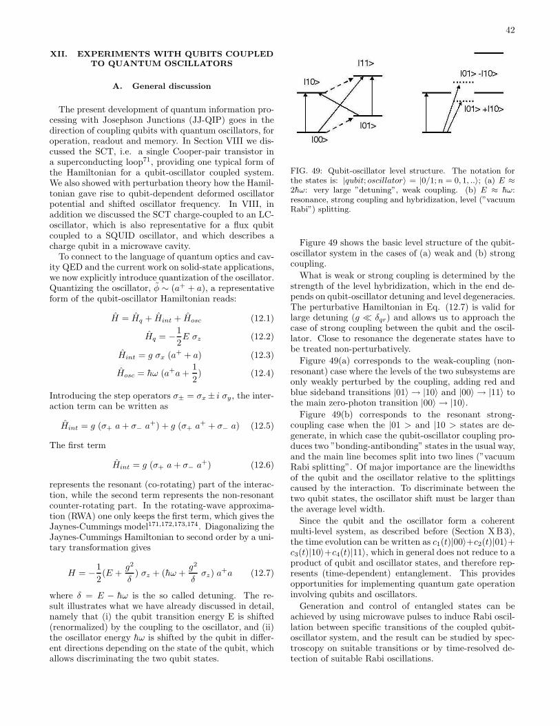
42

XII. EXPERIMENTS WITH QUBITS COUPLEDTO QUANTUM OSCILLATORS

A. General discussion

The present development of quantum information pro-cessing with Josephson Junctions (JJ-QIP) goes in thedirection of coupling qubits with quantum oscillators, foroperation, readout and memory. In Section VIII we dis-cussed the SCT, i.e. a single Cooper-pair transistor ina superconducting loop71, providing one typical form ofthe Hamiltonian for a qubit-oscillator coupled system.We also showed with perturbation theory how the Hamil-tonian gave rise to qubit-dependent deformed oscillatorpotential and shifted oscillator frequency. In VIII, inaddition we discussed the SCT charge-coupled to an LC-oscillator, which is also representative for a flux qubitcoupled to a SQUID oscillator, and which describes acharge qubit in a microwave cavity.

To connect to the language of quantum optics and cav-ity QED and the current work on solid-state applications,we now explicitly introduce quantization of the oscillator.Quantizing the oscillator, φ ∼ (a+ + a), a representativeform of the qubit-oscillator Hamiltonian reads:

H = Hq + Hint + Hosc (12.1)

Hq = −1

2E σz (12.2)

Hint = g σx (a+ + a) (12.3)

Hosc = hω (a+a+1

2) (12.4)

Introducing the step operators σ± = σx ± i σy, the inter-action term can be written as

Hint = g (σ+ a+ σ− a+) + g (σ+ a+ + σ− a) (12.5)

The first term

Hint = g (σ+ a+ σ− a+) (12.6)

represents the resonant (co-rotating) part of the interac-tion, while the second term represents the non-resonantcounter-rotating part. In the rotating-wave approxima-tion (RWA) one only keeps the first term, which gives theJaynes-Cummings model171,172,173,174. Diagonalizing theJaynes-Cummings Hamiltonian to second order by a uni-tary transformation gives

H = −1

2(E +

g2

δ) σz + (hω +

g2

δσz) a

+a (12.7)

where δ = E − hω is the so called detuning. The re-sult illustrates what we have already discussed in detail,namely that (i) the qubit transition energy E is shifted(renormalized) by the coupling to the oscillator, and (ii)the oscillator energy hω is shifted by the qubit in differ-ent directions depending on the state of the qubit, whichallows discriminating the two qubit states.

FIG. 49: Qubit-oscillator level structure. The notation forthe states is: |qubit; oscillator〉 = |0/1;n = 0, 1, ..〉; (a) E ≈2hω: very large ”detuning”, weak coupling. (b) E ≈ hω:resonance, strong coupling and hybridization, level (”vacuumRabi”) splitting.

Figure 49 shows the basic level structure of the qubit-oscillator system in the cases of (a) weak and (b) strongcoupling.

What is weak or strong coupling is determined by thestrength of the level hybridization, which in the end de-pends on qubit-oscillator detuning and level degeneracies.The perturbative Hamiltonian in Eq. (12.7) is valid forlarge detuning (g ≪ δqr) and allows us to approach thecase of strong coupling between the qubit and the oscil-lator. Close to resonance the degenerate states have tobe treated non-perturbatively.

Figure 49(a) corresponds to the weak-coupling (non-resonant) case where the levels of the two subsystems areonly weakly perturbed by the coupling, adding red andblue sideband transitions |01〉 → |10〉 and |00〉 → |11〉 tothe main zero-photon transition |00〉 → |10〉.

Figure 49(b) corresponds to the resonant strong-coupling case when the |01 > and |10 > states are de-generate, in which case the qubit-oscillator coupling pro-duces two ”bonding-antibonding” states in the usual way,and the main line becomes split into two lines (”vacuumRabi splitting”. Of major importance are the linewidthsof the qubit and the oscillator relative to the splittingscaused by the interaction. To discriminate between thetwo qubit states, the oscillator shift must be larger thanthe average level width.

Since the qubit and the oscillator form a coherentmulti-level system, as described before (Section XB3),the time evolution can be written as c1(t)|00〉+c2(t)|01〉+c3(t)|10〉+c4(t)|11〉, which in general does not reduce to aproduct of qubit and oscillator states, and therefore rep-resents (time-dependent) entanglement. This providesopportunities for implementing quantum gate operationinvolving qubits and oscillators.

Generation and control of entangled states can beachieved by using microwave pulses to induce Rabi oscil-lation between specific transitions of the coupled qubit-oscillator system, and the result can be studied by spec-troscopy on suitable transitions or by time-resolved de-tection of suitable Rabi oscillations.

43

FIG. 50: Resonant frequencies indicated by peaks in theSQUID switching probability when a long (300 ns) microwavepulse excites (saturates) the system before the readout pulse.Data are represented as a function of the external flux Φext

through the qubit area away from the qubit symmetry point.The blue |00〉 → |11〉 and red |01〉 → |10〉 sidebands are shownby down- and up-triangles, respectively; continuous lines areobtained by adding 2.96 GHz and -2.90 GHz, respectively,to the central continuous line (numerical fit). These valuesare close to the oscillator resonance frequency νp at 2.91 GHz(solid circles). Courtesy of J.E. Mooij, TU Delft.

B. Delft persistent current flux qubit coupled to aquantum oscillator

The Delft experiment25 demonstrates entanglementbetween a superconducting flux qubit and a SQUIDquantum oscillator. The SQUID provides the measure-ment system for detecting the quantum states (thresholdswitching detector, Fig. 44). It is also presents an effec-tive inductance that, in parallel with an external shuntcapacitance, acts as a low-frequency harmonic oscillator;the qubit and oscillator frequencies are approximatelyhνq = hν01 ≈ 6 GHz and hνr ≈ 3 GHz, correspondingto Fig. 49(a).

In the Delft experiment25, performing spectroscopy onthe coupled qubit-oscillator multi-level system reveals thevariation of the main and sideband transitions with fluxbias Φext, as shown in Fig. 50. The presence of visiblesideband transitions demonstrates the qubit-oscillator in-teraction and (weak) level hybridization).

Short microwave pulses can now be used to induce Rabioscillations between the various qubit-oscillator transi-tions. In the Delft experiment25, microwave pulses withfrequency νq = ν01 ≈ ∆/h ≈ 5.9 GHz (qubit symme-try point) were first used to induce Rabi oscillationswith ∼ 25 ns decay time at the main qubit transition|00〉 → |10〉 (and |01〉 → |11〉) for different values ofthe microwave power. The Rabi frequency as functionof the amplitude of the microwave voltage demonstratedqubit-oscillator hybridization (avoided crossings) at theoscillator νp (νr) and Larmor ∆/h (!) frequencies.

The dynamics of the coupled qubit-oscillator systemcan be studied by inducing microwave-driven Rabi oscil-lation between the blue |00〉 → |11〉 and red |01〉 → |10〉sidebands. In particular one can study the conditional

FIG. 51: Generation and control of entangled states via π and2π Rabi pulses on the qubit transition |00〉 → |10〉, followedby Rabi driving of blue sideband transitions |00〉 →. A π pulseexcites the system from |00〉 to |10〉, which suppresses the bluesideband transitions |00〉 → |11〉 (second curve from the top).On the other hand, with a 2π pulse the system returns to |00〉,which allows Rabi oscillation on the blue sideband. Adaptedfrom Chiorescu et al.25

dynamics in microwave multi-pulse experiments: by co-herently (de)populating selected levels via proper timingof Rabi oscillations induced by a first pulse, a secondpulse can induce Rabi oscillations on another transitionconnected to the levels controlled by the first pulse. Al-ternatively, such Rabi oscillations can instead be blockedby the first excitation.

This is shown experimentally in Fig. ??: by preparingthe initial state with initial π and 2π pulses, the side-band Rabi oscillations could be turned off and on again.The corresponding Rabi oscillations are shown in the leftpart of Fig. ??(b), demonstrating rapid decay due to thestrong damping of the SQUID oscillator (lifetime ∼ 3 ns;Q=100-150).

In the previous example, the control pulse (first pulse)was applied to the main |00〉 → |10〉 transition, control-ling the populations of the ”0” and ”1” levels. In thenext example, microwave control pulse is applied to the|00〉 → |01〉 transition, inducing Rabi oscillations whichpopulate the first excited state of oscillator. A secondmicrowave pulse (in principle, with different frequency)can then induce Rabi oscillations on the |01〉 → |10〉transition (red-sideband). The experimental result25 isshown Fig. 53, Clearly, for sufficiently long qubit and os-cillator lifetimes, one can prepare entangled Bell states,12 (|00〉 ± |01〉) and 1

2 (|01〉 ± |10〉) by applying π/2 mi-crowave pulses to the |00〉 → |11〉 and |01〉 → |10〉 tran-

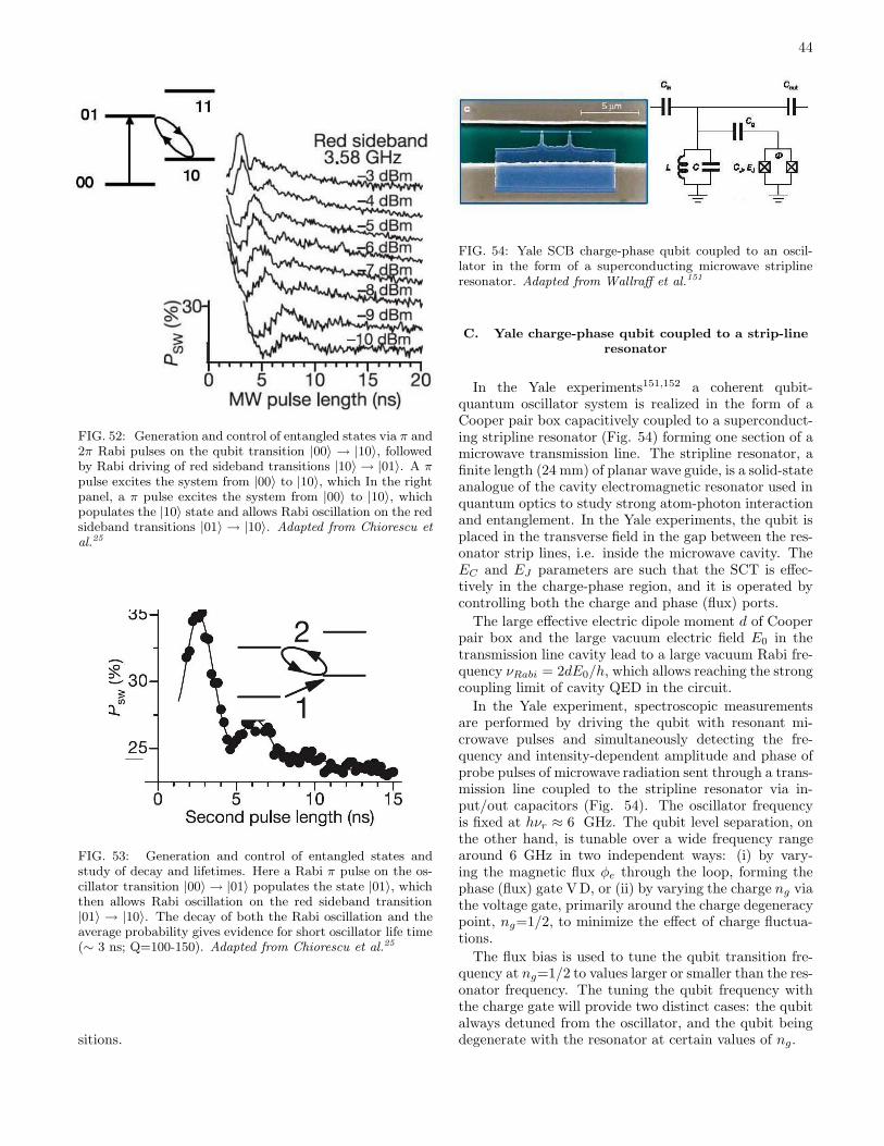
44

FIG. 52: Generation and control of entangled states via π and2π Rabi pulses on the qubit transition |00〉 → |10〉, followedby Rabi driving of red sideband transitions |10〉 → |01〉. A πpulse excites the system from |00〉 to |10〉, which In the rightpanel, a π pulse excites the system from |00〉 to |10〉, whichpopulates the |10〉 state and allows Rabi oscillation on the redsideband transitions |01〉 → |10〉. Adapted from Chiorescu etal.25

FIG. 53: Generation and control of entangled states andstudy of decay and lifetimes. Here a Rabi π pulse on the os-cillator transition |00〉 → |01〉 populates the state |01〉, whichthen allows Rabi oscillation on the red sideband transition|01〉 → |10〉. The decay of both the Rabi oscillation and theaverage probability gives evidence for short oscillator life time(∼ 3 ns; Q=100-150). Adapted from Chiorescu et al.25

sitions.

FIG. 54: Yale SCB charge-phase qubit coupled to an oscil-lator in the form of a superconducting microwave striplineresonator. Adapted from Wallraff et al.151

C. Yale charge-phase qubit coupled to a strip-lineresonator

In the Yale experiments151,152 a coherent qubit-quantum oscillator system is realized in the form of aCooper pair box capacitively coupled to a superconduct-ing stripline resonator (Fig. 54) forming one section of amicrowave transmission line. The stripline resonator, afinite length (24 mm) of planar wave guide, is a solid-stateanalogue of the cavity electromagnetic resonator used inquantum optics to study strong atom-photon interactionand entanglement. In the Yale experiments, the qubit isplaced in the transverse field in the gap between the res-onator strip lines, i.e. inside the microwave cavity. TheEC and EJ parameters are such that the SCT is effec-tively in the charge-phase region, and it is operated bycontrolling both the charge and phase (flux) ports.

The large effective electric dipole moment d of Cooperpair box and the large vacuum electric field E0 in thetransmission line cavity lead to a large vacuum Rabi fre-quency νRabi = 2dE0/h, which allows reaching the strongcoupling limit of cavity QED in the circuit.

In the Yale experiment, spectroscopic measurementsare performed by driving the qubit with resonant mi-crowave pulses and simultaneously detecting the fre-quency and intensity-dependent amplitude and phase ofprobe pulses of microwave radiation sent through a trans-mission line coupled to the stripline resonator via in-put/out capacitors (Fig. 54). The oscillator frequencyis fixed at hνr ≈ 6 GHz. The qubit level separation, onthe other hand, is tunable over a wide frequency rangearound 6 GHz in two independent ways: (i) by vary-ing the magnetic flux φe through the loop, forming thephase (flux) gate VD, or (ii) by varying the charge ng viathe voltage gate, primarily around the charge degeneracypoint, ng=1/2, to minimize the effect of charge fluctua-tions.

The flux bias is used to tune the qubit transition fre-quency at ng=1/2 to values larger or smaller than the res-onator frequency. The tuning the qubit frequency withthe charge gate will provide two distinct cases: the qubitalways detuned from the oscillator, and the qubit beingdegenerate with the resonator at certain values of ng.

45

A central result151 is the evidence for the qubit-oscillator hybridization and splitting of the degenerate|01〉 and |10〉 states, ν01 → ν±, as illustrated in Fig.49 (right). This splitting is often called ”vacuum Rabi”splitting because the ocillator is in its ground (vacuum)state.

The |01〉, |10〉 level splitting is observed through mi-crowave excitation of the 0 → 1 resonance transitionand observing the splitting of the resonance line as thequbit and the oscillator are tuned into resonance (by tun-ing the qubit frequency to zero qubit-oscillator detuning,δ = νq − νr = 0).

Another central result152 is the evidence for a longqubit dephasing time of T2 > 200 ns under optimal con-ditions: qubit parked at the charge degeneracy point,and weak driving field (low photon occupation numberin the resonator cavity). In the experiment151 the qubit-oscillator detuning is large, the qubit resonance transi-tion νq = ν01 is scanned by microwave radiation, and thedispersive shift of the resonator frequency νr seen by amicrowave probe beam is used to determine the occupa-tion of the qubit levels. Scanning the qubit |00〉 → |10〉resonance line profile allowed to determine the lineshapeand linewith as a function of microwave power, giving thebest value of T2 > 200 ns. Moreover, observation of thepostion of the resonance as a function of microwave powerallowed the determination of the ac-Stark shift, i.e. theRabi frequency as a function of the photon occupation(electric field) of the cavity. The measurement inducesan ac-Stark shift of 0.6 MHz per photon in the qubit levelseparation. Fluctuations in the photon number (shotnoise) induce level fluctuations in the qubit leading todephasing which is the characteristic back-action of themeasurement. A cross-over from Lorentzian to Gaus-sian resonance line shape with increasing measurementpower is observed and explained by dependence of theresonance linewidth on the cavity occupation number,exceeding the linewidth due to intrinsic decoherence athigh rf-power.

D. Comparison of the Delft and Yale approaches

In comparison, the Delft experiment25 corresponds tothe case of very large detuning (νq = 6 GHz, νr = 3 GHz;δ = νq − νr ∼ νr; Fig. 49 (left)), so that one will observea main resonance line |00〉 → |10〉 and two sidebands,|00〉 → |11〉 (blue) and |01〉 → |10〉 (red). Decreasing thedetuning δ, the blue and red sidebands will move awayto higher resp. lower frequencies, and one will arrive atthe case of zero detuning and qubit-oscillator degeneracy.If the qubit-oscillator coupling is larger than the averagelinewidth, one will then observe a splitting of the mainline (Fig. 49 (right)).

FIG. 55: The NEC 2-qubit system: two capacitively cou-pled charge qubits. The left qubit is a single Cooper pairbox (SCB) and the right qubit is an SCT with flux-tunableJosephson energy. Courtesy of J.S. Tsai, NEC, Tsukuba,Japan.

XIII. EXPERIMENTAL MANIPULATION OFCOUPLED TWO-QUBIT SYSTEMS

A. Capacitively coupled charge qubits

An AFM picture of the NEC SCB 2-qubit system36 isshown in Fig. 55 and the corresponding circuit JJ circuitin Fig. 28 (note that in the NEC circuit the left SCT isreplaced by a simple SCB).

Two coupled qubits constitute a 4-level system. TheHamiltonian for the NEC system of two capacitively cou-pled charge qubits (SCBs) was analyzed in the Appendix.The four energy eigenvalues E1,2,3,4(ng1, ng2) are plot-ted in Fig. 56 as a functions of the gate charges. Ateach point in the parameter space, an arbitrary two-qubitstate can be written as a superposition of the four two-qubit energy eigenstates.

As described in Sections IV and X, the general proce-dure for operating with dc-pulses is to initialize the sys-tem to its ground state |00〉 at the chosen starting point(ng10, ng20) and then suddenly change the Hamiltonianat time t = 0 to the gate bias (ng1, ng2). If the change isstrictly sudden, then the state at (ng1, ng2) at time t = 0is |ψ(t = 0)〉 = |00〉, which can be expanded in the energybasis of the Hamiltonian,

|ψ(0)〉 = |00〉 = c1|E1〉+ c2|E2〉+ c3|E3〉+ c4|E4〉 (13.1)

This stationary state then develops in time governed bythe constant Hamiltonian as

|ψ(t)〉 = c1e−iE1t|E1〉 + c2e

−iE2t|E2〉 +

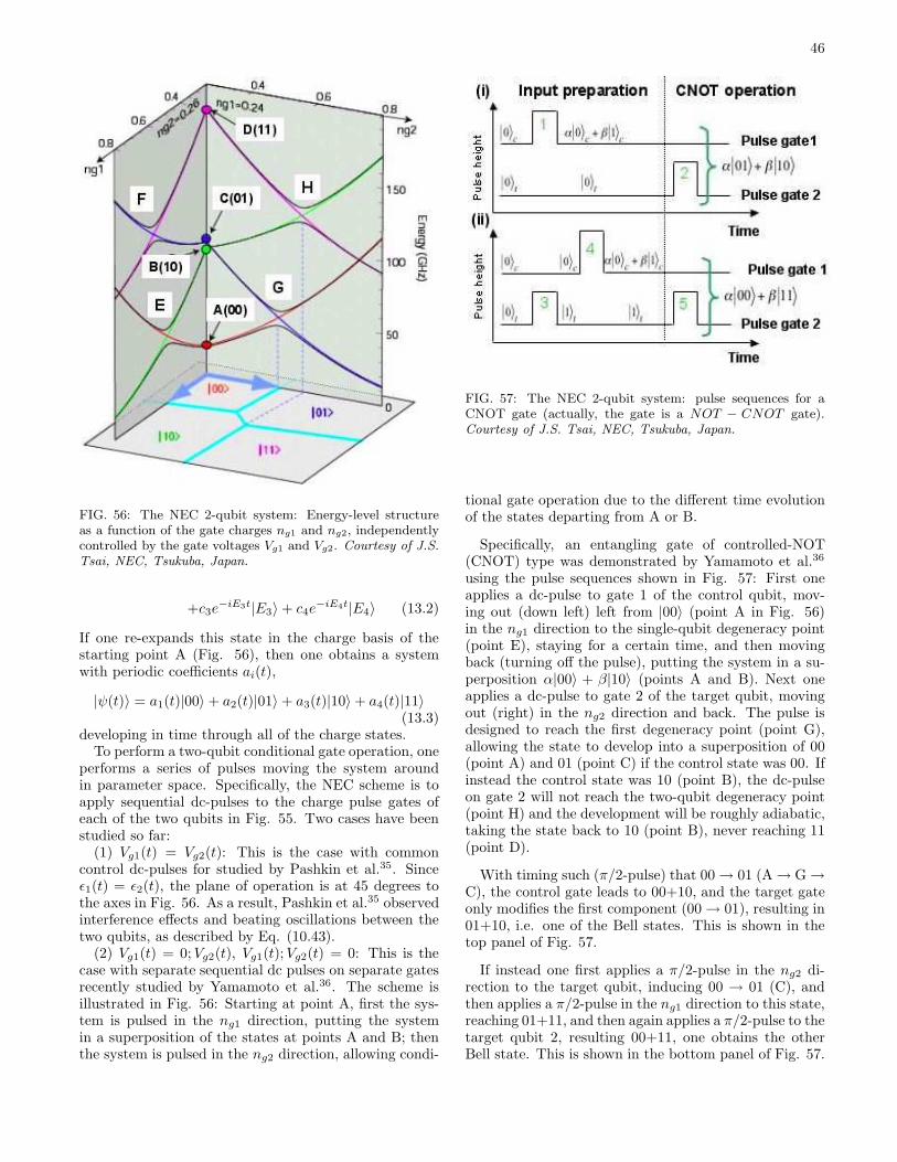
46

FIG. 56: The NEC 2-qubit system: Energy-level structureas a function of the gate charges ng1 and ng2, independentlycontrolled by the gate voltages Vg1 and Vg2. Courtesy of J.S.Tsai, NEC, Tsukuba, Japan.

+c3e−iE3t|E3〉 + c4e

−iE4t|E4〉 (13.2)

If one re-expands this state in the charge basis of thestarting point A (Fig. 56), then one obtains a systemwith periodic coefficients ai(t),

|ψ(t)〉 = a1(t)|00〉 + a2(t)|01〉 + a3(t)|10〉 + a4(t)|11〉(13.3)

developing in time through all of the charge states.To perform a two-qubit conditional gate operation, one

performs a series of pulses moving the system aroundin parameter space. Specifically, the NEC scheme is toapply sequential dc-pulses to the charge pulse gates ofeach of the two qubits in Fig. 55. Two cases have beenstudied so far:

(1) Vg1(t) = Vg2(t): This is the case with commoncontrol dc-pulses for studied by Pashkin et al.35. Sinceǫ1(t) = ǫ2(t), the plane of operation is at 45 degrees tothe axes in Fig. 56. As a result, Pashkin et al.35 observedinterference effects and beating oscillations between thetwo qubits, as described by Eq. (10.43).

(2) Vg1(t) = 0;Vg2(t), Vg1(t);Vg2(t) = 0: This is thecase with separate sequential dc pulses on separate gatesrecently studied by Yamamoto et al.36. The scheme isillustrated in Fig. 56: Starting at point A, first the sys-tem is pulsed in the ng1 direction, putting the systemin a superposition of the states at points A and B; thenthe system is pulsed in the ng2 direction, allowing condi-

FIG. 57: The NEC 2-qubit system: pulse sequences for aCNOT gate (actually, the gate is a NOT − CNOT gate).Courtesy of J.S. Tsai, NEC, Tsukuba, Japan.

tional gate operation due to the different time evolutionof the states departing from A or B.

Specifically, an entangling gate of controlled-NOT(CNOT) type was demonstrated by Yamamoto et al.36

using the pulse sequences shown in Fig. 57: First oneapplies a dc-pulse to gate 1 of the control qubit, mov-ing out (down left) left from |00〉 (point A in Fig. 56)in the ng1 direction to the single-qubit degeneracy point(point E), staying for a certain time, and then movingback (turning off the pulse), putting the system in a su-perposition α|00〉 + β|10〉 (points A and B). Next oneapplies a dc-pulse to gate 2 of the target qubit, movingout (right) in the ng2 direction and back. The pulse isdesigned to reach the first degeneracy point (point G),allowing the state to develop into a superposition of 00(point A) and 01 (point C) if the control state was 00. Ifinstead the control state was 10 (point B), the dc-pulseon gate 2 will not reach the two-qubit degeneracy point(point H) and the development will be roughly adiabatic,taking the state back to 10 (point B), never reaching 11(point D).

With timing such (π/2-pulse) that 00 → 01 (A → G →C), the control gate leads to 00+10, and the target gateonly modifies the first component (00 → 01), resulting in01+10, i.e. one of the Bell states. This is shown in thetop panel of Fig. 57.

If instead one first applies a π/2-pulse in the ng2 di-rection to the target qubit, inducing 00 → 01 (C), andthen applies a π/2-pulse in the ng1 direction to this state,reaching 01+11, and then again applies a π/2-pulse to thetarget qubit 2, resulting 00+11, one obtains the otherBell state. This is shown in the bottom panel of Fig. 57.

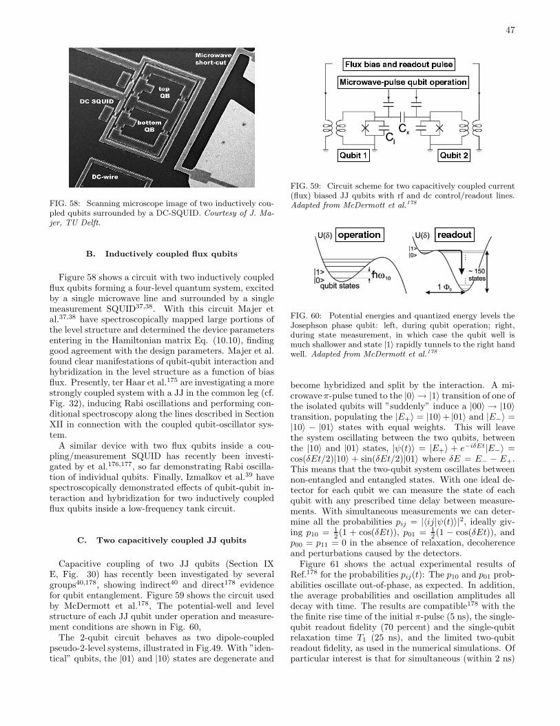
47

FIG. 58: Scanning microscope image of two inductively cou-pled qubits surrounded by a DC-SQUID. Courtesy of J. Ma-jer, TU Delft.

B. Inductively coupled flux qubits

Figure 58 shows a circuit with two inductively coupledflux qubits forming a four-level quantum system, excitedby a single microwave line and surrounded by a singlemeasurement SQUID37,38. With this circuit Majer etal.37,38 have spectroscopically mapped large portions ofthe level structure and determined the device parametersentering in the Hamiltonian matrix Eq. (10.10), findinggood agreement with the design parameters. Majer et al.found clear manifestations of qubit-qubit interaction andhybridization in the level structure as a function of biasflux. Presently, ter Haar et al.175 are investigating a morestrongly coupled system with a JJ in the common leg (cf.Fig. 32), inducing Rabi oscillations and performing con-ditional spectroscopy along the lines described in SectionXII in connection with the coupled qubit-oscillator sys-tem.

A similar device with two flux qubits inside a cou-pling/measurement SQUID has recently been investi-gated by et al.176,177, so far demonstrating Rabi oscilla-tion of individual qubits. Finally, Izmalkov et al.39 havespectroscopically demonstrated effects of qubit-qubit in-teraction and hybridization for two inductively coupledflux qubits inside a low-frequency tank circuit.

C. Two capacitively coupled JJ qubits

Capacitive coupling of two JJ qubits (Section IXE, Fig. 30) has recently been investigated by severalgroups40,178, showing indirect40 and direct178 evidencefor qubit entanglement. Figure 59 shows the circuit usedby McDermott et al.178, The potential-well and levelstructure of each JJ qubit under operation and measure-ment conditions are shown in Fig. 60,

The 2-qubit circuit behaves as two dipole-coupledpseudo-2-level systems, illustrated in Fig.49. With ”iden-tical” qubits, the |01〉 and |10〉 states are degenerate and

FIG. 59: Circuit scheme for two capacitively coupled current(flux) biased JJ qubits with rf and dc control/readout lines.Adapted from McDermott et al.178

FIG. 60: Potential energies and quantized energy levels theJosephson phase qubit: left, during qubit operation; right,during state measurement, in which case the qubit well ismuch shallower and state |1〉 rapidly tunnels to the right handwell. Adapted from McDermott et al.178

become hybridized and split by the interaction. A mi-crowave π-pulse tuned to the |0〉 → |1〉 transition of one ofthe isolated qubits will ”suddenly” induce a |00〉 → |10〉transition, populating the |E+〉 = |10〉+ |01〉 and |E−〉 =|10〉 − |01〉 states with equal weights. This will leavethe system oscillating between the two qubits, betweenthe |10〉 and |01〉 states, |ψ(t)〉 = |E+〉 + e−iδEt|E−〉 =cos(δEt/2)|10〉 + sin(δEt/2)|01〉 where δE = E− − E+.This means that the two-qubit system oscillates betweennon-entangled and entangled states. With one ideal de-tector for each qubit we can measure the state of eachqubit with any prescribed time delay between measure-ments. With simultaneous measurements we can deter-mine all the probabilities pij = |〈ij|ψ(t)〉|2, ideally giv-ing p10 = 1

2 (1 + cos(δEt)), p01 = 12 (1 − cos(δEt)), and

p00 = p11 = 0 in the absence of relaxation, decoherenceand perturbations caused by the detectors.

Figure 61 shows the actual experimental results ofRef.178 for the probabilities pij(t): The p10 and p01 prob-abilities oscillate out-of-phase, as expected. In addition,the average probabilities and oscillation amplitudes alldecay with time. The results are compatible178 with thethe finite rise time of the initial π-pulse (5 ns), the single-qubit readout fidelity (70 percent) and the single-qubitrelaxation time T1 (25 ns), and the limited two-qubitreadout fidelity, as used in the numerical simulations. Ofparticular interest is that for simultaneous (within 2 ns)

48

FIG. 61: Interaction of the coupled qubits in the time do-main. The qubits are tuned into resonance and the systemis suddenly prepared in state (10) by a microwave π-pulseapplied to qubit 1. Simultaneous single-shot measurementof each of the qubits 1 and 2 reads out the probabilitiesp00, p10, p01, p11 for finding the 1+2 system in states 00, 10,01, and 11, respectively. The full lines represent results ofnumerical simulations. Adapted from McDermott et al.178

readout of the qubits, the experiments show that readoutof one qubit only leads to small perturbation of the otherqubit178, which is promising for multi-qubit applications.

XIV. QUANTUM STATE ENGINEERING WITHMULTI-QUBIT JJ SYSTEMS

Due to the recent experimental progress, protocolsand algorithms for multi-qubit JJ systems can soonbegin to be implemented in order to test the perfor-mance of JJ qubit and readout circuits and to studythe full dynamics of the quantum systems. The gen-eral principles are well known (see e.g.49,50) and havevery recently been successfully applied in several othersystems to achieve interesting and significant resultsin well-controlled quantum systems: ion-trap technol-ogy has been used to entangle 4 qubits180, implement2-qubit gates and test Bell’s inequalities181,184, per-form the Deutsch-Josza algorithm182, achieve telepor-tation (within the system)185,186,187, and perform er-ror correction188; quantum optics has recently demon-strated long-distance teleportation190 as well as 4-photonentanglement190,191. There are presently a considerabletheoretical literature on how to implement these and sim-ilar protocols and algorithms in JJ circits. Below we willdescribe a few examples to illustrate what may need tobe done experimentally.

FIG. 62: EPR anticorrelation in the singlet state

A. Bell measurements

The first essential step is to study the quantum dy-namics of a two-qubit circuit and to perform a test ofBell’s inequalities by creating entangled two-qubit Bellstates (Section III, Ref.49) and performing simultaneousprojective measurements on the two qubits, similarly tothe ion trap experiments181,184. Clearly the experimentwill be a test of the quantum properties of the circuitand the measurement process rather than a test of a Bellinequality.

The general principle is to (a) entangle the two qubits,(b) measure the projection along different detector axes(”polarization directions”), (c) perform four independentmeasurements, and finally (d) analyze the correlations. Ifthe detector axes are fixed, as is the case for the JJ read-out (measuring charge or flux), one can instead rotateeach of the qubits.

Figure 62 shows the quantum network for creating aBell state |ψ〉, perform single qubit rotations Rx(φ1),Rx(φ2), and finally perform a projective measurement oneach of the qubits along the same common fixed quan-tization axis. For each setting of the angles, (φ1, φ2),on then performs a series of measurements obtaining theprobabilities Pij = |〈ij|ψ〉|2 = 〈ψ|ij〉〈ij|ψ〉. These canbe combined into the results for finding the two qubitsin the same state, Psame = P00 + P11, or in differentstates, Pdiff = P01 + P10, and finally into the differenceq(φ1, φ2) = Psame−Pdiff . This quantity q(φ1, φ2) is eval-uated in four experiments for two independent settingsof the two angles, φ1 = (α, δ), φ2 = (β, γ), constructingthe function

B(α, δ;β, γ) = |q(α, β) + q(δ, β)| (14.1)

+|q(α, γ) − q(δ, γ)|

The Clauser-Horne-Shimony-Holt (CSCH)condition192 for violation of classical physics is thenB > 2 (maximum value 2

√2).

The application to JJ charge-phase qubits has beendiscussed by Refs.193,194. Experimentally, a first stepin this direction has been taken by Martinis et al.178

who directly detected the anticorrelation in the oscillat-ing superposition of Bell states |ψ(t)〉 = cos(δEt/2)|10〉+sin(δEt/2)|01〉.

49

FIG. 63: Teleportation in a 3-qubit system. The unknownqubit (1) to be teleported is |ψ〉 = a|0〉 + b|1〉. The resultof the measurement is sent by Alice via classical channels toBob who performs the appropriate unitary transformations torestore the original single-qubit state. As a result of the tele-portation, a specific but unknown state has been transferredfrom one qubit to another.

B. Teleportation

In the simplest form of teleportation an unknownsingle-qubit quantum state is transferred from one partof the system to another, i.e. from one qubit to another,as illustrated in Fig. 63. In Fig. 63, the initial state isgiven by

(a|0〉 + b|1〉)(|00〉) (14.2)

Next, applying CNOT and Hadamard gates entanglesqubits 2 and 3 into a Bell state,

(a|0〉 + b|1〉)(1/ ∗ 2)(|00〉 + |11〉) (14.3)

which is the resource needed for teleportation (in quan-tum optics this corresponds to the entangled photon pairshared between Alice and Bob). One member of the Bellpair (qubit 2) is now ”sent” to Alice and entangled withthe unknown qubit to be teleported, creating a 3-qubitentangled state,

|00〉(a|0〉 + b|1〉) (14.4)

+ |01〉(b|0〉 + a|1〉)+ |10〉(a|0〉 − b|1〉)

+ |11〉(−b|0〉 + a|1〉)

At this point, qubit 3 is sent to Bob, meaning that a 3-qubit entangled state is shared between Alice and Bob.Moreover, at this point, in each component of this 3-qubitentangled state in Eq. (14.4), the two upper qubits are ineigenstates. This means that a projective measurementof the these two qubits by Alice will collapse the totalstate to one of the four components. If the result ofAlice’s measurement is (ij), the first two qubits are inthe state |ij〉 and the 3-qubit state is known, given bythe corresponding component in the previous equation.Any of these 3-qubit products can be transformed by a

FIG. 64: Teleportation in a 3-qubit system without measure-ment and classical transmission. The unknown qubit (1) to betransferred is again |ψ〉 = a|0〉+b|1〉. The state of qubits 1 and2 are now used to control CNOT gates to restore the originalsingle-qubit state on qubit 3. As a result of the teleportation,a specific but unknown state has been transferred from qubit1 to qubit 3, leaving qubits 1 and 2 in superposition states.

unitary transformation back to the original state:

I(a|0〉 + b|1〉) = |ψ〉 (14.5)

σx(b|0〉 + a|1〉) = |ψ〉 (14.6)

σz(a|0〉 − b|1〉) = |ψ〉 (14.7)

σzσx(−b|0〉 + a|1〉) = |ψ〉 (14.8)

corresponding to resp. no change, bit flip, phase flipand bit-plus-phase flip of the original unknown state |ψ〉.Alice’s measurement causes instantaneous collapse, afterwhich Alice by classical means (e.g. e-mail!) can tellBob which unitary transformation to apply to recoverthe original single-qubit state.

An alternative approach, without measurement andclassical transmission, is shown in Fig. 64, In this case,the final 3-qubit state is still a disentangled product statewith the correct state |ψ〉 = a|0〉 + b|1〉 on qubit 3,

1√2(|0〉 + |1〉) 1√

2(|0〉 + |1〉)(a|0〉 + b|1〉) (14.9)

while qubits 1 and 2 are now in superposition states. Ifdesired, these states can be rotated back to |00〉 by singlequbit gates.

The teleportation protocol has been implemented inion trap experiments186,187 (and of course in quantumoptics189). A proposal for a setup for implementing ateleportation scheme in JJ circuitry is shown in Fig. 65,describing a 3-qubit chain of charge-phase qubits coupledby current-biased large JJ oscillators, in principle allow-ing controllable nearest-neighbour qubit couplings158,159:In the absence of bias currents, to first order the qubitsare non-interacting and isolated from each other. Thebasic two-qubit gates are achieved by switching on thebias-current-controlled qubit-qubit interaction for a giventime. CNOT gates can be achieved in combination withsingle-qubit Hadamard and phase gates158,159,160. By ap-plying the sequence of gates shown in Fig. 64 (or anequivalent sequence), the unknown state will be physi-cally moved from the left end to the right end of the chain.Moreover, by applying coupling pulses simultaneously to

50

φb

i−2φb φb

i−1 i

I bi

Ii−1b gi

gi

φ φφ2(i−1)

φ φ1i 2i 1(i+1) 2(i+1)

φ1(i−1)

Qubit i−1 Qubit i Qubit i+1

C

V

FIG. 65: Network of loop-shaped SCT charge qubits, coupledby large Josephson junctions. The interaction of the qubits(i) and (i + 1) is controlled by the current bias Ibi Individ-ual qubits are controlled by voltage gates, Vgi. Single-qubitreadout is performed by applying an ac current pulse to a par-ticular JJ readout junction (not shown), or using an RF-SETcapacitively coupled to the island [27].

several qubits, one can in principle create multi-qubitentangled states in fewer operations than with sequentialtwo-qubit gates195,196 as well as perform operations inparallel on different parts of the system.

Extending the system to a five-qubit chain one can ina similar way transfer an entangled two-qubit state fromthe left to the right end of the chain.

C. Qubit buses and entanglement transfer

With entangled ”flying qubits” like photons, quan-tum correlations can be shared in a spatially highly ex-tended states. However, with solid-state circuitry theissue becomes how to transfer entanglement among spa-tially fixed qubits.

The standard answer is to apply entangling two-qubitgates between distant qubits. The qubit-qubit interac-tion can be direct, e.g. dipole-dipole-type interaction be-tween distant qubits, or mediated by excitations in thesystem. The transfer can be mediated via virtual or realexcitations in a passive polarizable medium, a ”systembus”, or via a protocol for coupling qubits and bus oscil-lators.

A classic example of protocol-controlled oscillator-mediated coupling is the Cirac-Zoller gate197 betweentwo ions sequentially entangled via exchange couplingwith the lowest vibrational mode of the ions in the trap.Another example is the Molmer-Sorensen gate198,199,200

which creates qubit-qubit interaction via virtual ex-citation of ion-trap modes. Similar concepts forcontrolling entanglement have recently been theoreti-cally investigated in applications to JJ-qubit-oscillatorcircuits164,201,202,203,204,205,206,207,208

An different approach is to allow the bus (”spin-chain”)states to develop in time governed by the fixed bus Hamil-tonian and to tailor the interactions and the initital con-ditions such that useful dynamics and information trans-fer is achieved209,210,211,212. Also these concepts havebeen applied to JJ-circuits in a number of recent the-

FIG. 66: Teleportation with error correction in a 5-qubitsystem without measurement.

FIG. 67: Coding, decoding and correcting a bit flip error ina 3-qubit logic qubit. The first gate on the left represents twosequential CNOT gates. The last gate befor the garbage canis a control-control-NOT (Toffoli) gate.

oretical studies213,214,215,216,217,218,219.

D. Qubit encoding and quantum error correction

Quantum error correction (QEC) (see e.g.Refs.49,220,221,222,223,224,225,226) will most certainlybe necessary for successful operation of solid state quan-tum information devices in order to fight decoherence.The algorithmic approach to QEC follows the principlesof classical error correction, by encoding bits to createredundancy, and by devising procedures for identifyingand correcting the errors based on specific models forthe errors.

The quantum circuit in Fig. 66 illustrates QEC interms of five-qubit teleportation with bit errors, illus-trating restoration of the state including error correctionby measurement-controlled unitary transformation.

The quantum circuit in Fig. 67 demonstrates someessential steps of QEC in the case of one logical qubitencoded in three physical qubits: The first step is toencode the physical qubit in logical qubit basis states|000〉 and |111〉 by applying two CNOT gates to create a3-qubit entangled state:

(a|0〉 + b|1〉) |00〉 → (a|000〉 + b|111〉) (14.10)

Next, there may occur a bit-flip error in one of the qubits:

a|000〉 + b|111〉 (no bit f lip) (14.11)

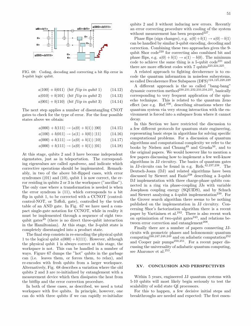
51

FIG. 68: Coding, decoding and correcting a bit flip error in3-qubit logic qubit.

a|100〉 + b|011〉 (bit f lip in qubit 1) (14.12)

a|010〉 + b|101〉 (bit f lip in qubit 2) (14.13)

a|001〉 + b|110〉 (bit f lip in qubit 3) (14.14)

The next step applies a number of disentangling CNOTgates to check for the type of error. For the four possiblestates above we obtain:

a|000〉 + b|111〉 → (a|0〉 + b|1〉) |00〉 (14.15)

a|100〉 + b|011〉 → (a|1〉 + b|0〉) |11〉 (14.16)

a|000〉 + b|111〉 → (a|0〉 + b|1〉) |10〉 (14.17)

a|000〉 + b|111〉 → (a|0〉 + b|1〉) |01〉 (14.18)

At this stage, qubits 2 and 3 have become independenteigenstates, just as in teleportation. The correspond-ing eigenvalues are called syndrome, and indicate whichcorrective operations should be implemented. Remark-ably, in two of the above bit-flipped cases, with errorsyndromes ((01) and (10), qubit 1 is now correct, the er-ror residing in qubits 2 or 3 in the workspace (”ancillas”).The only case where a transformation is needed is whenthe error syndrom is (11), which corresponds to a bitflip in qubit 1, to be corrected with a CCNOT (control-control-NOT, or Toffoli, gate), controlled by the truthtable of an AND gate. In Fig. 67 we have used a com-pact single-gate notation for CCNOT, while in reality itmust be implemented through a sequence of eight two-qubit gates49 (there is no direct three-qubit interactionin the Hamiltonian). At this stage, the 3-qubit state iscompletely disentangled into a product state.

The final step consists in re-encoding the physical qubit1 to the logical qubit a|000〉+ b|111〉. However, althoughthe physical qubit 1 is always correct at this stage, theworkspace is not. This can be handled in a number ofways. Figure 67 dumps the ”hot” qubits in the garbagecan (i.e. leaves them, or forces them, to relax), andre-encodes with fresh qubits from a larger workspace.Alternatively, Fig. 68 describes a variation where the oldqubits 2 and 3 are re-initialized by entanglement with ameasurement device which then dissipates the heat fromthe bitflip and the error correction procedure.

In both of these cases, as described, we need a totalworkspace with five qubits. In principle, however, onecan do with three qubits if we can rapidly re-initialize

qubits 2 and 3 without inducing new errors. Recentlyan error correcting procedure with cooling of the systemwithout measurement has been proposed227.

Phase flips (sign changes), e.g. a|0〉+b|1〉 → a|0〉−b|1〉can be handled by similar 3-qubit encoding, decoding andcorrection. Combining these two approaches gives the 9-qubit Shor code220 for correcting also combined bit andphase flips, e.g. a|0〉 + b|1〉 → a|1〉 − b|0〉. The minimumcode to achieve the same thing is a 5-qubit code221 andthere are more efficient codes with 7 qubits223,224,225.

A related approach to fighting decoherence is to en-code the quantum information in noiseless subsystems,so called Decoherence Free Subspaces (DFS)124,125,228,229

A different approach is the so called ”bang-bang”dynamic correction method230,231,232,233,234,235, basicallycorresponding to very frequent application of the spin-echo technique. This is related to the quantum Zenoeffect (see e.g. Ref.236, describing situations where thequantum system via very strong interaction with the en-vironment is forced into a subspace from where it cannotdecay.

In this Section we have restricted the discussion toa few different protocols for quantum state engineering,representing basic steps in algorithms for solving specificcomputational problems. For a discussion of quantumalgorithms and computational complexity we refer to thebooks by Nielsen and Chuang49 and Gruska50, and tothe original papers. We would however like to mention afew papers discussing how to implement a few well-knowalgorithms in JJ circuitry. The basics of quantum gatesin JJ-circuits can be found in e.g. Refs.42,237,238. TheDeutsch-Josza (DJ) and related algorithms have beendiscussed by Siewert and Fazio238 describing a 3-qubitDJ implementation with three charge-phase qubits con-nected in a ring via phase-coupling JJs with variableJosephson coupling energy (SQUIDS), and by Schuchand Siewert analyzing a 4-qubit implementation239. Forthe Grover search algorithm there seems to be nothingpublished on the implementation in JJ circuitry. Con-cerning Shor’s factorization algorithm there is a recentpaper by Vartiainen et al.242. There is also recent workon optimization of two-qubit gates243, and relations be-tween error correction and entanglement208.

Finally there are a number of papers connecting JJ-ciruits wih geometric phases and holononomic quantumcomputing246,247,248,249 and on adiabatic computation252

and Cooper pair pumps250,251. For a recent paper dis-cussing the universality of adiabatic quantum computing,see Aharonov et al.253.

XV. CONCLUSION AND PERSPECTIVES

Within 5 years, engineered JJ quantum systems with5-10 qubits will most likely begin seriously to test thescalability of solid state QI processors.

For this to happen, a few decisive initial steps andbreakthroughs are needed and expected: The first essen-

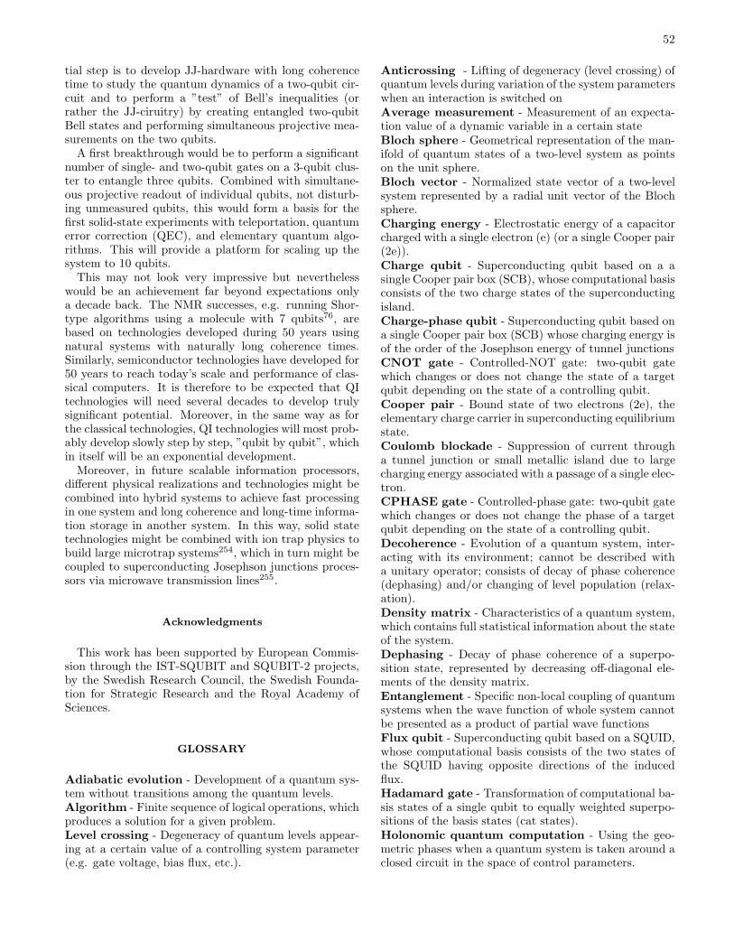
52

tial step is to develop JJ-hardware with long coherencetime to study the quantum dynamics of a two-qubit cir-cuit and to perform a ”test” of Bell’s inequalities (orrather the JJ-ciruitry) by creating entangled two-qubitBell states and performing simultaneous projective mea-surements on the two qubits.

A first breakthrough would be to perform a significantnumber of single- and two-qubit gates on a 3-qubit clus-ter to entangle three qubits. Combined with simultane-ous projective readout of individual qubits, not disturb-ing unmeasured qubits, this would form a basis for thefirst solid-state experiments with teleportation, quantumerror correction (QEC), and elementary quantum algo-rithms. This will provide a platform for scaling up thesystem to 10 qubits.

This may not look very impressive but neverthelesswould be an achievement far beyond expectations onlya decade back. The NMR successes, e.g. running Shor-type algorithms using a molecule with 7 qubits76, arebased on technologies developed during 50 years usingnatural systems with naturally long coherence times.Similarly, semiconductor technologies have developed for50 years to reach today’s scale and performance of clas-sical computers. It is therefore to be expected that QItechnologies will need several decades to develop trulysignificant potential. Moreover, in the same way as forthe classical technologies, QI technologies will most prob-ably develop slowly step by step, ”qubit by qubit”, whichin itself will be an exponential development.

Moreover, in future scalable information processors,different physical realizations and technologies might becombined into hybrid systems to achieve fast processingin one system and long coherence and long-time informa-tion storage in another system. In this way, solid statetechnologies might be combined with ion trap physics tobuild large microtrap systems254, which in turn might becoupled to superconducting Josephson junctions proces-sors via microwave transmission lines255.

Acknowledgments

This work has been supported by European Commis-sion through the IST-SQUBIT and SQUBIT-2 projects,by the Swedish Research Council, the Swedish Founda-tion for Strategic Research and the Royal Academy ofSciences.

GLOSSARY

Adiabatic evolution - Development of a quantum sys-tem without transitions among the quantum levels.Algorithm - Finite sequence of logical operations, whichproduces a solution for a given problem.Level crossing - Degeneracy of quantum levels appear-ing at a certain value of a controlling system parameter(e.g. gate voltage, bias flux, etc.).

Anticrossing - Lifting of degeneracy (level crossing) ofquantum levels during variation of the system parameterswhen an interaction is switched onAverage measurement - Measurement of an expecta-tion value of a dynamic variable in a certain stateBloch sphere - Geometrical representation of the man-ifold of quantum states of a two-level system as pointson the unit sphere.Bloch vector - Normalized state vector of a two-levelsystem represented by a radial unit vector of the Blochsphere.Charging energy - Electrostatic energy of a capacitorcharged with a single electron (e) (or a single Cooper pair(2e)).Charge qubit - Superconducting qubit based on a asingle Cooper pair box (SCB), whose computational basisconsists of the two charge states of the superconductingisland.Charge-phase qubit - Superconducting qubit based ona single Cooper pair box (SCB) whose charging energy isof the order of the Josephson energy of tunnel junctionsCNOT gate - Controlled-NOT gate: two-qubit gatewhich changes or does not change the state of a targetqubit depending on the state of a controlling qubit.Cooper pair - Bound state of two electrons (2e), theelementary charge carrier in superconducting equilibriumstate.Coulomb blockade - Suppression of current througha tunnel junction or small metallic island due to largecharging energy associated with a passage of a single elec-tron.CPHASE gate - Controlled-phase gate: two-qubit gatewhich changes or does not change the phase of a targetqubit depending on the state of a controlling qubit.Decoherence - Evolution of a quantum system, inter-acting with its environment; cannot be described witha unitary operator; consists of decay of phase coherence(dephasing) and/or changing of level population (relax-ation).Density matrix - Characteristics of a quantum system,which contains full statistical information about the stateof the system.Dephasing - Decay of phase coherence of a superpo-sition state, represented by decreasing off-diagonal ele-ments of the density matrix.Entanglement - Specific non-local coupling of quantumsystems when the wave function of whole system cannotbe presented as a product of partial wave functionsFlux qubit - Superconducting qubit based on a SQUID,whose computational basis consists of the two states ofthe SQUID having opposite directions of the inducedflux.Hadamard gate - Transformation of computational ba-sis states of a single qubit to equally weighted superpo-sitions of the basis states (cat states).Holonomic quantum computation - Using the geo-metric phases when a quantum system is taken around aclosed circuit in the space of control parameters.

53

Gate operation - Controlled transformation of the stateof one or several qubits; a basic element of an algorithm.Josephson effect - Non-dissipative current flow be-tween two superconductors separated by a non-superconducting material (insulator, normal metal, etc.).Josephson junction - Junction of two superconductors,which exhibits the Josephson effect.Josephson critical current - Maximal value of theJosephson current maintained by a particular junction.Josephson energy - Inductive energy of a Josephsonjunction proportional to the critical Josephson current.π pulse - High frequency control pulse with a specificduration applied to a qubit, producing inversion of thequbit level populations (π rotation; qubit flip)π/2 pulse - High frequency control pulse with a specificduration applied to a qubit, typically tipping the Blochvector from a pole to the equator, or from the equator toa pole, on the Bloch sphere.Phase gate - Single qubit gate, transforms a superpo-sition of two quantum states into another superpositionwith different relative phase of the statesPrecession - Dynamic evolution of a two-level system ina superposition state, i.e. linear combination of energyeigenstates.QND measurement - Quantum Non-Demolition Mea-surement: measurement of a state of a quantum system,which does not destroy the quantum state and makespossible repeated measurements of the same state.QPC - Quantum Point Contact: a constriction in a con-ductor with ballistic transport through a small numberof conduction channels.Qubit - Quantum two-level system; basic element of aquantum processor.PCQ - Persistent Current Qubit: synonymous with fluxqubit.Rabi oscillation - Dynamics of two-level system under

resonant driving perturbation, consists of periodic oscil-lation of the level populations with the frequency propor-tional to the amplitude of the perturbation.Readout - Measurement of a qubit state.Relaxation - Change of population of the energy eigen-states resulting in approaching the equilibrium popula-tion.SCB - Single Cooper pair Box: superconducting analogof SEB, where it is energetically favorable to have onlypaired electrons on the island.SCT - Single Cooper pair Transistor: a superconductingdevice containing a small island whose charging energy iscontrolled by an electrostatic gate electrode to increaseor decrease current flowing through the island from onelarge electrode (source) to another (drain).SEB - Single Electron Box: small metallic island con-nected to a large electrode via resistive tunnel junction,whose charging energy hence amount of trapped electronsis controlled by an electrostatic gate.SET - Single Electron Transistor: a device containing asmall island whose charging energy is controlled by anelectrostatic gate electrode to increase or decrease cur-rent flowing through the island from one large electrode(source) to another (drain).rf-SET - SET driven by an rf signal, is used as an ul-tra sensitive electrometer by monitoring a linear responsefunction of the SET, which is sensitive to the electrostaticgate potential.SQUID - Superconducting Quantum Interferometer De-vice: a device consisting of a one or more Josephson junc-tions included in a superconducting loop.dc-SQUID - SQUID containing two Josephson junc-tions.rf-SQUID - SQUID containing one Josephson junction.Single-shot measurement - A measurement whichgives an ”up/down” answer in one single detection event.

1 Y. Nakamura, Yu. Pashkin and J.S. Tsai: ”Coherent con-trol of macroscopic quantum states in a single-Cooper-pairbox”, Nature 398, 786 (1999).

2 A.O. Caldeira and A. Legget: ”Influence of dissipation onquantum tunneling in macroscopic systems”, Phys. Rev.Lett. 46, 211 (1981).

3 A.J. Legget et al.: ”Dynamics of the dissipative two-statesystem”, Rev. Mod. Phys. 59, 1 (1987).

4 M.H. Devoret, J.M. Martinis and J. Clarke: ”Measurementsof macroscopic quantum tunneling out of the zero-voltagestate of a current-biased Josephson junction”, Phys. Rev.Lett. 55, 1908 (1985).

5 J. Clarke, A.N. Cleland, M.H. Devoret, D. Esteve and J.M.Martinis: ”Quantum mechanics of a macroscopic variable:the phase difference of a Josephson junction”, Science 239,992 (1988).

6 J.E. Mooij, T.P. Orlando, L. Levitov, Lin Tian, C.H.van der Wal, and S. Lloyd: ”Josephson persistent currentqubit”, Science 285, 1036 (1999).

7 C.H. van der Wal, A.C.J. ter Haar, F. Wilhelm, R.N.

Schouten, C.J.P.M. Harmans, T.P. Orlando, S. LloydJ.E. and Mooij: ”Quantum superposition of macroscopicpersistent-current states”, Science 290, 773 (2000).

8 J.R. Friedman, V. Patel, W. Chen, S.K. Tolpygo and J.E.Lukens: ”Detection of a Schrodinger’s cat state in an rf-SQUID”, Nature 406, 43 (2000).

9 K.K. Likharev: ”Dynamics of Josephson junctions and cir-cuits”, Gordon and Breach (1986).

10 K.K. Likharev, Y. Naveh and D. Averin: ”Physics of high-jc Josephson junctions and prospects of their RSFQ VLSIapplications”, IEEE Trans. on Appl. Supercond. 11, 1056(2001).

11 K. Gaj, E.G. Friedman and M.J Feldman: ”Timing ofmulti-gighertz rapid single flux quantum digital circuits”,J. VLSI Signal Processing 16, 247 (1997).

12 K.K. Likharev and A. Zorin: ”Theory of Bloch-wave oscil-lations in small Josephson junctions”, J. Low. Temp. Phys.59 347 (1985).

13 V. Bouchiat, P. Joyez, H. Pothier, C. Urbina, D. Es-teve, and M.H. Devoret: ”Quantum coherence with a single

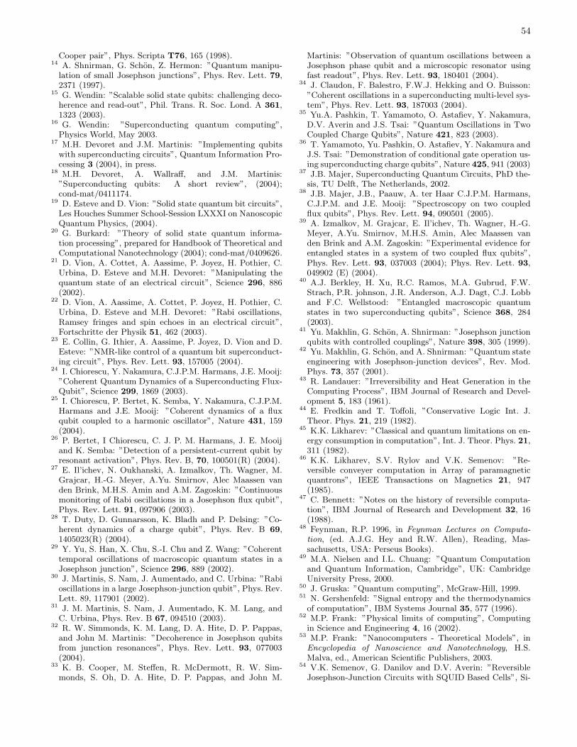
54

Cooper pair”, Phys. Scripta T76, 165 (1998).14 A. Shnirman, G. Schon, Z. Hermon: ”Quantum manipu-

lation of small Josephson junctions”, Phys. Rev. Lett. 79,2371 (1997).

15 G. Wendin: ”Scalable solid state qubits: challenging deco-herence and read-out”, Phil. Trans. R. Soc. Lond. A 361,1323 (2003).

16 G. Wendin: ”Superconducting quantum computing”,Physics World, May 2003.

17 M.H. Devoret and J.M. Martinis: ”Implementing qubitswith superconducting circuits”, Quantum Information Pro-cessing 3 (2004), in press.

18 M.H. Devoret, A. Wallraff, and J.M. Martinis:”Superconducting qubits: A short review”, (2004);cond-mat/0411174.

19 D. Esteve and D. Vion: ”Solid state quantum bit circuits”,Les Houches Summer School-Session LXXXI on NanoscopicQuantum Physics, (2004).

20 G. Burkard: ”Theory of solid state quantum informa-tion processing”, prepared for Handbook of Theoretical andComputational Nanotechnology (2004); cond-mat/0409626.

21 D. Vion, A. Cottet, A. Aassime, P. Joyez, H. Pothier, C.Urbina, D. Esteve and M.H. Devoret: ”Manipulating thequantum state of an electrical circuit”, Science 296, 886(2002).

22 D. Vion, A. Aassime, A. Cottet, P. Joyez, H. Pothier, C.Urbina, D. Esteve and M.H. Devoret: ”Rabi oscillations,Ramsey fringes and spin echoes in an electrical circuit”,Fortschritte der Physik 51, 462 (2003).

23 E. Collin, G. Ithier, A. Aassime, P. Joyez, D. Vion and D.Esteve: ”NMR-like control of a quantum bit superconduct-ing circuit”, Phys. Rev. Lett. 93, 157005 (2004).

24 I. Chiorescu, Y. Nakamura, C.J.P.M. Harmans, J.E. Mooij:”Coherent Quantum Dynamics of a Superconducting Flux-Qubit”, Science 299, 1869 (2003).

25 I. Chiorescu, P. Bertet, K. Semba, Y. Nakamura, C.J.P.M.Harmans and J.E. Mooij: ”Coherent dynamics of a fluxqubit coupled to a harmonic oscillator”, Nature 431, 159(2004).

26 P. Bertet, I Chiorescu, C. J. P. M. Harmans, J. E. Mooijand K. Semba: ”Detection of a persistent-current qubit byresonant activation”, Phys. Rev. B, 70, 100501(R) (2004).

27 E. Il’ichev, N. Oukhanski, A. Izmalkov, Th. Wagner, M.Grajcar, H.-G. Meyer, A.Yu. Smirnov, Alec Maassen vanden Brink, M.H.S. Amin and A.M. Zagoskin: ”Continuousmonitoring of Rabi oscillations in a Josephson flux qubit”,Phys. Rev. Lett. 91, 097906 (2003).

28 T. Duty, D. Gunnarsson, K. Bladh and P. Delsing: ”Co-herent dynamics of a charge qubit”, Phys. Rev. B 69,1405023(R) (2004).

29 Y. Yu, S. Han, X. Chu, S.-I. Chu and Z. Wang: ”Coherenttemporal oscillations of macroscopic quantum states in aJosephson junction”, Science 296, 889 (2002).

30 J. Martinis, S. Nam, J. Aumentado, and C. Urbina: ”Rabioscillations in a large Josephson-junction qubit”, Phys. Rev.Lett. 89, 117901 (2002).

31 J. M. Martinis, S. Nam, J. Aumentado, K. M. Lang, andC. Urbina, Phys. Rev. B 67, 094510 (2003).

32 R. W. Simmonds, K. M. Lang, D. A. Hite, D. P. Pappas,and John M. Martinis: ”Decoherence in Josephson qubitsfrom junction resonances”, Phys. Rev. Lett. 93, 077003(2004).

33 K. B. Cooper, M. Steffen, R. McDermott, R. W. Sim-monds, S. Oh, D. A. Hite, D. P. Pappas, and John M.

Martinis: ”Observation of quantum oscillations between aJosephson phase qubit and a microscopic resonator usingfast readout”, Phys. Rev. Lett. 93, 180401 (2004).

34 J. Claudon, F. Balestro, F.W.J. Hekking and O. Buisson:”Coherent oscillations in a superconducting multi-level sys-tem”, Phys. Rev. Lett. 93, 187003 (2004).

35 Yu.A. Pashkin, T. Yamamoto, O. Astafiev, Y. Nakamura,D.V. Averin and J.S. Tsai: ”Quantum Oscillations in TwoCoupled Charge Qubits”, Nature 421, 823 (2003).

36 T. Yamamoto, Yu. Pashkin, O. Astafiev, Y. Nakamura andJ.S. Tsai: ”Demonstration of conditional gate operation us-ing superconducting charge qubits”, Nature 425, 941 (2003)

37 J.B. Majer, Superconducting Quantum Circuits, PhD the-sis, TU Delft, The Netherlands, 2002.

38 J.B. Majer, J.B., Paauw, A. ter Haar C.J.P.M. Harmans,C.J.P.M. and J.E. Mooij: ”Spectroscopy on two coupledflux qubits”, Phys. Rev. Lett. 94, 090501 (2005).

39 A. Izmalkov, M. Grajcar, E. Il’ichev, Th. Wagner, H.-G.Meyer, A.Yu. Smirnov, M.H.S. Amin, Alec Maassen vanden Brink and A.M. Zagoskin: ”Experimental evidence forentangled states in a system of two coupled flux qubits”,Phys. Rev. Lett. 93, 037003 (2004); Phys. Rev. Lett. 93,049902 (E) (2004).

40 A.J. Berkley, H. Xu, R.C. Ramos, M.A. Gubrud, F.W.Strach, P.R. johnson, J.R. Anderson, A.J. Dagt, C.J. Lobband F.C. Wellstood: ”Entangled macroscopic quantumstates in two superconducting qubits”, Science 368, 284(2003).

41 Yu. Makhlin, G. Schon, A. Shnirman: ”Josephson junctionqubits with controlled couplings”, Nature 398, 305 (1999).

42 Yu. Makhlin, G. Schon, and A. Shnirman: ”Quantum stateengineering with Josephson-junction devices”, Rev. Mod.Phys. 73, 357 (2001).

43 R. Landauer: ”Irreversibility and Heat Generation in theComputing Process”, IBM Journal of Research and Devel-opment 5, 183 (1961).

44 E. Fredkin and T. Toffoli, ”Conservative Logic Int. J.Theor. Phys. 21, 219 (1982).

45 K.K. Likharev: ”Classical and quantum limitations on en-ergy consumption in computation”, Int. J. Theor. Phys. 21,311 (1982).

46 K.K. Likharev, S.V. Rylov and V.K. Semenov: ”Re-versible conveyer computation in Array of paramagneticquantrons”, IEEE Transactions on Magnetics 21, 947(1985).

47 C. Bennett: ”Notes on the history of reversible computa-tion”, IBM Journal of Research and Development 32, 16(1988).

48 Feynman, R.P. 1996, in Feynman Lectures on Computa-tion, (ed. A.J.G. Hey and R.W. Allen), Reading, Mas-sachusetts, USA: Perseus Books).

49 M.A. Nielsen and I.L. Chuang: ”Quantum Computationand Quantum Information, Cambridge”, UK: CambridgeUniversity Press, 2000.

50 J. Gruska: ”Quantum computing”, McGraw-Hill, 1999.51 N. Gershenfeld: ”Signal entropy and the thermodynamics

of computation”, IBM Systems Journal 35, 577 (1996).52 M.P. Frank: ”Physical limits of computing”, Computing

in Science and Engineering 4, 16 (2002).53 M.P. Frank: ”Nanocomputers - Theoretical Models”, in

Encyclopedia of Nanoscience and Nanotechnology, H.S.Malva, ed., American Scientific Publishers, 2003.

54 V.K. Semenov, G. Danilov and D.V. Averin: ”ReversibleJosephson-Junction Circuits with SQUID Based Cells”, Si-

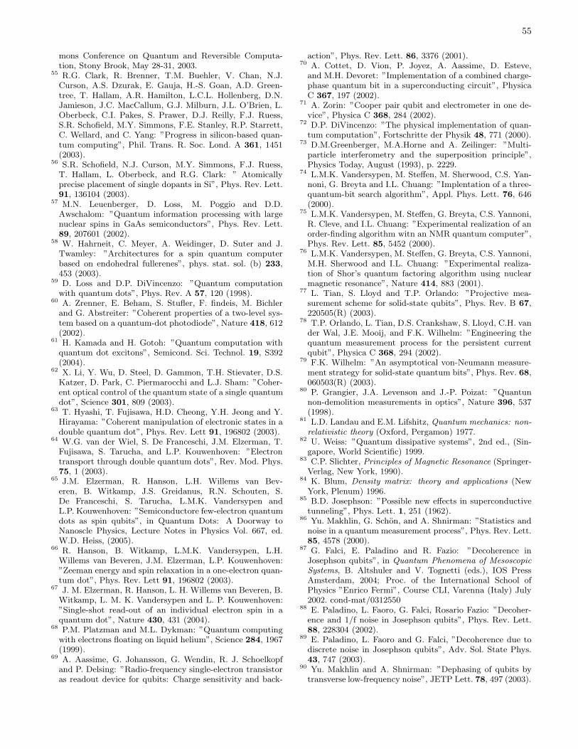
55

mons Conference on Quantum and Reversible Computa-tion, Stony Brook, May 28-31, 2003.

55 R.G. Clark, R. Brenner, T.M. Buehler, V. Chan, N.J.Curson, A.S. Dzurak, E. Gauja, H.-S. Goan, A.D. Green-tree, T. Hallam, A.R. Hamilton, L.C.L. Hollenberg, D.N.Jamieson, J.C. MacCallum, G.J. Milburn, J.L. O’Brien, L.Oberbeck, C.I. Pakes, S. Prawer, D.J. Reilly, F.J. Ruess,S.R. Schofield, M.Y. Simmons, F.E. Stanley, R.P. Starrett,C. Wellard, and C. Yang: ”Progress in silicon-based quan-tum computing”, Phil. Trans. R. Soc. Lond. A 361, 1451(2003).

56 S.R. Schofield, N.J. Curson, M.Y. Simmons, F.J. Ruess,T. Hallam, L. Oberbeck, and R.G. Clark: ” Atomicallyprecise placement of single dopants in Si”, Phys. Rev. Lett.91, 136104 (2003).

57 M.N. Leuenberger, D. Loss, M. Poggio and D.D.Awschalom: ”Quantum information processing with largenuclear spins in GaAs semiconductors”, Phys. Rev. Lett.89, 207601 (2002).

58 W. Hahrneit, C. Meyer, A. Weidinger, D. Suter and J.Twamley: ”Architectures for a spin quantum computerbased on endohedral fullerenes”, phys. stat. sol. (b) 233,453 (2003).

59 D. Loss and D.P. DiVincenzo: ”Quantum computationwith quantum dots”, Phys. Rev. A 57, 120 (1998).

60 A. Zrenner, E. Beham, S. Stufler, F. findeis, M. Bichlerand G. Abstreiter: ”Coherent properties of a two-level sys-tem based on a quantum-dot photodiode”, Nature 418, 612(2002).

61 H. Kamada and H. Gotoh: ”Quantum computation withquantum dot excitons”, Semicond. Sci. Technol. 19, S392(2004).

62 X. Li, Y. Wu, D. Steel, D. Gammon, T.H. Stievater, D.S.Katzer, D. Park, C. Piermarocchi and L.J. Sham: ”Coher-ent optical control of the quantum state of a single quantumdot”, Science 301, 809 (2003).

63 T. Hyashi, T. Fujisawa, H.D. Cheong, Y.H. Jeong and Y.Hirayama: ”Coherent manipulation of electronic states in adouble quantum dot”, Phys. Rev. Lett 91, 196802 (2003).

64 W.G. van der Wiel, S. De Franceschi, J.M. Elzerman, T.Fujisawa, S. Tarucha, and L.P. Kouwenhoven: ”Electrontransport through double quantum dots”, Rev. Mod. Phys.75, 1 (2003).

65 J.M. Elzerman, R. Hanson, L.H. Willems van Bev-eren, B. Witkamp, J.S. Greidanus, R.N. Schouten, S.De Franceschi, S. Tarucha, L.M.K. Vandersypen andL.P. Kouwenhoven: ”Semiconductore few-electron quantumdots as spin qubits”, in Quantum Dots: A Doorway toNanoscle Physics, Lecture Notes in Physics Vol. 667, ed.W.D. Heiss, (2005).

66 R. Hanson, B. Witkamp, L.M.K. Vandersypen, L.H.Willems van Beveren, J.M. Elzerman, L.P. Kouwenhoven:”Zeeman energy and spin relaxation in a one-electron quan-tum dot”, Phys. Rev. Lett 91, 196802 (2003).

67 J. M. Elzerman, R. Hanson, L. H. Willems van Beveren, B.Witkamp, L. M. K. Vandersypen and L. P. Kouwenhoven:”Single-shot read-out of an individual electron spin in aquantum dot”, Nature 430, 431 (2004).

68 P.M. Platzman and M.L. Dykman: ”Quantum computingwith electrons floating on liquid helium”, Science 284, 1967(1999).

69 A. Aassime, G. Johansson, G. Wendin, R. J. Schoelkopfand P. Delsing: ”Radio-frequency single-electron transistoras readout device for qubits: Charge sensitivity and back-

action”, Phys. Rev. Lett. 86, 3376 (2001).70 A. Cottet, D. Vion, P. Joyez, A. Aassime, D. Esteve,

and M.H. Devoret: ”Implementation of a combined charge-phase quantum bit in a superconducting circuit”, PhysicaC 367, 197 (2002).

71 A. Zorin: ”Cooper pair qubit and electrometer in one de-vice”, Physica C 368, 284 (2002).

72 D.P. DiVincenzo: ”The physical implementation of quan-tum computation”, Fortschritte der Physik 48, 771 (2000).

73 D.M.Greenberger, M.A.Horne and A. Zeilinger: ”Multi-particle interferometry and the superposition principle”,Physics Today, August (1993), p. 2229.

74 L.M.K. Vandersypen, M. Steffen, M. Sherwood, C.S. Yan-noni, G. Breyta and I.L. Chuang: ”Implentation of a three-quantum-bit search algorithm”, Appl. Phys. Lett. 76, 646(2000).

75 L.M.K. Vandersypen, M. Steffen, G. Breyta, C.S. Yannoni,R. Cleve, and I.L. Chuang: ”Experimental realization of anorder-finding algorithm witn an NMR quantum computer”,Phys. Rev. Lett. 85, 5452 (2000).

76 L.M.K. Vandersypen, M. Steffen, G. Breyta, C.S. Yannoni,M.H. Sherwood and I.L. Chuang: ”Experimental realiza-tion of Shor’s quantum factoring algorithm using nuclearmagnetic resonance”, Nature 414, 883 (2001).

77 L. Tian, S. Lloyd and T.P. Orlando: ”Projective mea-surement scheme for solid-state qubits”, Phys. Rev. B 67,220505(R) (2003).

78 T.P. Orlando, L. Tian, D.S. Crankshaw, S. Lloyd, C.H. vander Wal, J.E. Mooij, and F.K. Wilhelm: ”Engineering thequantum measurement process for the persistent currentqubit”, Physica C 368, 294 (2002).

79 F.K. Wilhelm: ”An asymptotical von-Neumann measure-ment strategy for solid-state quantum bits”, Phys. Rev. 68,060503(R) (2003).

80 P. Grangier, J.A. Levenson and J.-P. Poizat: ”Quantunnon-demolition measurements in optics”, Nature 396, 537(1998).

81 L.D. Landau and E.M. Lifshitz, Quantum mechanics: non-relativistic theory (Oxford, Pergamon) 1977.

82 U. Weiss: ”Quantum dissipative systems”, 2nd ed., (Sin-gapore, World Scientific) 1999.

83 C.P. Slichter, Principles of Magnetic Resonance (Springer-Verlag, New York, 1990).

84 K. Blum, Density matrix: theory and applications (NewYork, Plenum) 1996.

85 B.D. Josephson: ”Possible new effects in superconductivetunneling”, Phys. Lett. 1, 251 (1962).

86 Yu. Makhlin, G. Schon, and A. Shnirman: ”Statistics andnoise in a quantum measurement process”, Phys. Rev. Lett.85, 4578 (2000).

87 G. Falci, E. Paladino and R. Fazio: ”Decoherence inJosephson qubits”, in Quantum Phenomena of MesoscopicSystems, B. Altshuler and V. Tognetti (eds.), IOS PressAmsterdam, 2004; Proc. of the International School ofPhysics ”Enrico Fermi”, Course CLI, Varenna (Italy) July2002. cond-mat/0312550

88 E. Paladino, L. Faoro, G. Falci, Rosario Fazio: ”Decoher-ence and 1/f noise in Josephson qubits”, Phys. Rev. Lett.88, 228304 (2002).

89 E. Paladino, L. Faoro and G. Falci, ”Decoherence due todiscrete noise in Josephson qubits”, Adv. Sol. State Phys.43, 747 (2003).

90 Yu. Makhlin and A. Shnirman: ”Dephasing of qubits bytransverse low-frequency noise”, JETP Lett. 78, 497 (2003).

56

91 Yu. Makhlin, and A. Shnirman: ”Dephasing of solid-statequbits at optimal points”, Phys. Rev. Lett. 92, 178301(2004).

92 A. Shnirman, D. Mozyrsky, and I. Martin: ”Output noiseof a measuring device at arbitrary voltage and tempera-ture”, Europhys. Lett. 67, 840 (2004).

93 G. Falci, A. D’Arrigo, A. Mastellone and E. Paladino: ”Ini-tial decoherence in solid state qubits”, cond-mat/0409422.

94 F.K. Wilhelm, G. Schon, and G.T. Zimanyi, ”Supercon-ducting single-charge transistor in a tunable dissipative en-vironment”, Phys. Rev. Lett. 87, 136802 (2001).

95 F.K. Wilhelm, M.J. Storcz, C.H. van der Wal, C.J.P.M.Harmans, and J.E. Mooij: ”Decoherence of flux qubits cou-pled to electronic circuits”, Adv. Sol. St. Phys. 43, 763(2003).

96 M.C. Goorden and F.K. Wilhelm: ”Theoretical analysis ofcontinuously driven Josephson qubits”, Phys. Rev. B 68,012508 (2003).

97 C.H. van der Wal, F.K. Wilhelm, C.J.P.M. Harmans, J.E.Mooij: ”Engineering decoherence in Josephson persistent-current qubits”, European Physics Journal B 31, 111(2003).

98 K. W. Lehnert, B. A. Turek, K. Bladh, L. F. Spietz, D.Gunnarsson, P. Delsing, and R. J.Schoelkopf: ”Quantumcharge fluctuations and the polarizability of the single elec-tron box”, Phys. Rev. Lett. 91, 106801 (2003).

99 K. W. Lehnert, K. Bladh, L. F. Spietz, D. Gunnarsson, D.I. Schuster, P. Delsing and R. J. Schoelkopf: ”Measurementof the excited-state lifetime of a microelectronic circuit”,Phys. Rev. Lett. 90, 027002 (2003).

100 L. Roschier, P. Hakonen, K. Bladh, P. Delsing, K. Lehn-ert, L. Spietz, and R. Schoelkopf: ”Noise performance ofthe RF-SET”, J. Appl. Phys. 95, 1274 (2004).

101 G. Burkard, D.P. DiVincenzo, P. Bertet, I. Chiorescu, andJ. E. Mooij: ”Asymmetry and decoherence in a double-layerpersistent-current qubit”, Phys. Rev. B 71, 134504 (2005).

102 P. Bertet, I. Chiorescu, G. Burkard, K. Semba, C.J.P.M.Harmans, D.P. DiVincenzo, and J. E. Mooij: ”Relaxationand dephasing in a flux qubit”, (2004); cond-mat/0412485

103 P. Bertet, I. Chiorescu, C.J.P.M. Harmans and J. E.Mooij: ”Dephasing of a flux qubit coupled to a harmonicoscillator”, (2005); cond-mat/0507290.

104 D.V. Averin and R. Fazio: ”Active suppression of dephas-ing in Josephson-junction qubits”, JETP Lett. 78, 1162(2003).

105 A. Zazunov, V.S. Shumeiko, G. Wendin and E.N. Bra-tus: ”Dynamics and phonon-induced decoherence of An-dreev level qubits”, Phys. Rev. B 71, 214505 (2005).

106 M. Governale, M. Grifoni, and G. Schon: ”Decoher-ence and dephasing in coupled Josephson-junction qubits”,Chem. Phys. 268, 273 (2001).

107 M.J. Storcz und F.K. Wilhelm: ”Decoherence and gateperformance of coupled solid state qubits”, Phys. Rev. A67, 042319 (2003).

108 K. Rabenstein, V.A. Sverdlov and D.V. Averin: ”Qubitdecoherence by Gaussian low-frequency noise”, ZhETFLett. 79, 783 (2004); cond-mat/0401519.

109 K. Rabenstein and D.V. Averin: ”Decoherence intwo coupled qubits”, Turk. J. Phys. 27, 1 (2003);cond-mat/0310193.

110 L.B. Ioffe, V.B. Geshkenbein, Ch. Helm and G. Batter:”Decoherence in superconducting quantum bits by phononradiation”, Phys. Rev. Lett. 93, 057001 (2004).

111 P.G. deGennes, Superconductivity of Metals and Alloys

(New York, W.A. Benjamin) 1966.112 M. Tinkham, Introduction to superconductivity (New

York, McGraw Hill) 1996.113 A. Barone and G. Paterno, Physics and applications of

the Josephson effect (New York, Wiley) 1982.114 M.A. Kastner: ”The single-electron transistor”, Rev.

Mod. Phys. 64, 849 (1992).115 I. Giaever and H.R. Zeller: ”Tunneling, zero-bias anoma-

lies, and small superconductors”, Phys.Rev.Lett. 20, 1504(1968).

1 I.O. Kulik and R.I Shekhter: ”Kinetic phenomenaand charge discreteness effects in granulated media”,Sov.Phys.JETP 41, 308 (1975).

116 P. Lafarge, P. Joyez, D. Esteve, C. Urbina, and M. H. De-voret: ”Measurement of the even-odd free-energy differenceof an isolated superconductor”, Phys. Rev. Lett. 70, 994(1993).

117 P. Lafarge, P. Joyez, D. Esteve, C. Urbina, and M. H.Devoret: ”Two-electron quantization of the charge on a su-perconductor”, Nature 365, 422 (1993).

118 Single Charge Tunneling, Ed. H. Grabert and M.H. De-voret, NATO ASI Series (Plenum Press, New York) 1992.

119 Y. Nakamura Y., Yu.A. Pashkin and J.S. Tsai: ”Rabi Os-cillations in a Josephson-Junction Charge Two-Level Sys-tem”, Phys. Rev. Lett. 87, 246601 (2002).

120 Nakamura Y., Pashkin Yu. A., and Tsai J. S.: ”ChargeEcho in a Cooper-Pair Box”, Phys. Rev. Lett. 88, 047901(2002).

121 Mahn-Soo Choi, R. Fazio, J. Siewert, and C. Bruder: ”Co-herent oscillations in a Cooper-pair box”, Europhys. Lett.53, 251 (2001).

122 A.J. Leggett and A. Garg: ”Quantum mechanics versusmacroscopic realism: Is the flux there when nobody looks?”,Phys. Rev. Lett. 54, 857 (1985).

123 J.M. Martinis, M.H. Devoret, and J. Clarke: ”Experimen-tal tests for the quantum behavior of a macroscopic degreeof freedom: The phase difference across a Josephson junc-tion”, Phys.Rev.B 35, 4682 (1987).

124 L.B. Ioffe, M.V. Feigel’man, A. Ioselevich, D. Ivanov, MTroyer and G. Blatter: ”Topologically protected quantumbits using Josephson junction arrays”, Nature, 415, 503(2002).

125 M.V. Feigel’man, L.B. Ioffe, V.B. Geshkenbein, P. Dayal,and G. Blatter: ”Superconducting tetrahedral Quantumbits”, Phys. Rev. Lett. 92, 098301 (2004).

126 A. Zazunov, V.S. Shumeiko, E. Bratus, J. Lantz, andG. Wendin: ”Andreev level qubit”, Phys. Rev. Lett. 90,0870031 (2003).

127 A. Furusaki and M. Tsukada:”Unified theory of cleanJosephson junctions”, Physica B 165-166, 967 (1990).

128 V.S. Shumeiko, G. Wendin, and E.N. Bratus’: ”Reso-nance excitation of superconducting bound states in a tun-nel junction by an electromagnetic field: nonlinear responseof the Josephson current”, Phys. Rev. B 48, 13129 (1993).

129 V.S. Shumeiko, E.N. Bratus’, and G. Wendin: ”Dynamicsof Andreev level qubits, in: Electronic correlations: frommeso- to nano-physics”, Proceedings of XXXIII MoriondConference, ed. T. Martin, G. Montamboux, J.T. ThanhVan, EDP Sciences, 2001.

130 J. Lantz, V.S. Shumeiko, E.N. Bratus’, and G. Wendin,Flux qubit with a quantum point contact, Physica C, 368,315 (2002).

131 Yu-Xi Liu, L.F. Wei and F. Nori: ”Quantum tomographyfor solid state qubits”, Europhys. Lett. 67, 874 (2004).

57

132 D.V Averin: ”Continuous weak measurement of themacroscopic quantum coherent oscillations”, Fortschritteder Physik 48, 1055 (2000).

133 M.H. Devoret and R.J. Shoelkopf: ”Amplifying quantumsignals with the single-electron transistor”, Nature 406,1039 (2000).

134 R.J. Schoelkopf, P. Wahlgren, A.A. Kozhevnikov, P. Dels-ing and D.E. Prober: ”The radio-frequency single-electrontransistor (rf-SET): A fast and ultra-sensititive electrome-ter”, Science 280, 1238 (1998).

135 A. Aassime, D. Gunnarsson, K. Bladh, R.S. Schoelkopf,and P. Delsing: ”Radio frequency single electron transistortowards the quantum limit”, Appl. Phys. Lett. 79, 4031(2001).

136 O. Astafiev, Yu. A. Pashkin, T. Yamamoto, Y. Nakamura,and J. S. Tsai: ”Single-shot measurement of the Josephsoncharge qubit”, Phys. Rev. B 69, 180507(R) (2004).

137 G. Johansson, A. Kack, and G. Wendin: ”Full frequencyback-action spectrum of a single electron transistor duringqubit read-out”, Phys. Rev. Lett. 88, 046802 (2002).

138 A. Kack, G. Johansson and G. Wendin: ”Full frequencyvoltage-noise spectral density of a single electron transis-tor”, Phys. Rev B 67, 035301 (2003).

139 A.N. Korotkov and D.V. Averin: ”Continuous weak mea-surement of quantum coherent oscillations”, Phys. Rev. B64, 165310 (2001).

140 D.V. Averin: ”Quantum nondemolition measurements ofa qubit”, Phys. Rev. Lett. 88, 207901 (2002).

141 H.-S. Goan, G.J. Milburn, H.M. Wiseman and H.B. Sun:”Continuous quantum measurement of two coupled quan-tum dots using a point contact: A quantum trajectory ap-proach”, Phys. Rev. B 63, 125326 (2001).

142 H.-S. Goan and G. J. Milburn: ”Dynamcis of a mesoscopicqubit under continuous quantum measurement”, Phys. Rev.B 64, 235307 (2001).

143 A.L. Shelankov and J. Rammer: ”Charge transfer count-ing statistics revisited”, Europhysics Letters 63, 485 (2003).

144 J. Rammer, A.L. Shelankov, J. Wabnig: ”Quantum mea-surement in the charge representation”, Phys. Rev. B 70,115327 (2004).

145 F.W.J. Hekking, O. Buisson, F. Balestro and M.G.Vergniory: ”Cooper pair box coupled to a current-biasedJosephson junction”, in: Electronic correlations: frommeso- to nano-physics”, Proceedings of XXXIII MoriondConference, ed. T. Martin, G. Montamboux, J.T. ThanhVan, EDP Sciences, 2001, p.515.

146 F. Marquardt and C. Bruder: ”Superposition of two meso-scopically distinct quantum states: Coupling a Cooper-pirbox to a large superconducting island”, Phys. Rev. 63,054514 (2001).

147 S.M. Girvin, Ren-Shou Huang, Alexandre Blais, An-dreas Wallraff and R. J. Schoelkopf: ”Prospects of strongcavity quantum electrodynamics with superconducting cir-cuits”, Proceedings of Les Houches Summer School, SessionLXXIX, Quantum Entanglement and Information Process-ing (2003); cond-mat/0310670

148 A. Blais, R.-S. Huang, A. Wallraff, S. M. Girvin R. J.Schoelkopf: ”Cavity quantum electrodynamics for super-conducting electrical circuits: an architecture for quantumcomputation”, Phys. Rev. A 69, 062320 (2004).

149 I. Rau, G. Johansson, and A. Shnirman: ”Cavity QED insuperconducting circuits: susceptibility at elevated temper-atures”, Phys. Rev. B 70, 054521 (2004).

150 L. Roschier, M. Sillanpaa and P. Hakonen: ”Quantum

cpacitive phasse detector”, Phys. Rev. B 71, 024530 (2005).151 A. Wallraff, D. Schuster, A. Blais, L. Frunzo, R.-S. Huang,

J. Majer, S. Kumar, S.M. Girvin and R. J. Schoelkopf:”Cavity quantum electrodynamics: Coherent coupling ofa single photon to a Cooper pair box”, Nature 431, 165(2004).

152 D.I. Schuster, A. Wallraff, A. Blais, L. Frunzio, R.-S.Huang, J. Majer, S.M. Girvin and R.J. Schoelkopf: ”AC-Stark Shift and Dephasing of a Superconducting QubitStrongly Coupled to a Cavity Field”, Phys. Rev. Lett. 94,123602 (2005).

153 A. Wallraff, D. Schuster, A. Blais, L. Frunzo, J. Majer,S.M. Girvin and R. J. Schoelkopf: ”Approaching unit visi-bility for control of a superconducting qubit with dispersivereadout”, (2005); cond-mat/0502645.

154 J. Siewert, R. Fazio, G. M. Palma and E. Sciacca: ”As-pects of qubit dynamics in the presence of leakage”, Low.Temp. Phys. 118, 795 (2000).

155 J.Q. You, J.S. Tsai, J.S., F. Nori: ”Scalabale quantumcomputing with Josephson charge qubits”, Phys. Rev. Lett.89, 197902 (2002).

156 J.Q. You, J.S. Tsai, F. Nori: ”Controllable manipulationand entanglement of macroscopic quantum states in coupledcharge qubits”, Phys. Rev. B 68, 024510 (2003).

157 Y.D. Wang, P. Zhang, D.L. Zhou and C.P. Sun: ”Fastentanglement of two charge-phase qubits through non-adiabatic coupling to a large junction”, Ohys. Rev. B 70,224515 (2004).

158 J. Lantz, M. Wallquist, V.S. Shumeiko and G. Wendin:”Josephson junction qubit network with current-controlledinteraction”, Phys. Rev. B 70 140507(R) (2004).

159 M. Wallquist, J. Lantz, V.S. Shumeiko and G. Wendin:”Current-controlled coupling of superconducting chargequbits”, in Quantum Computation: solid state systems,eds. P. Delsing, C. Granata, Y. Pashkin, B. Ruggiero and P.Silvestrini, Kluwer Academic Plenum Publishers, December2005, in press.

160 M. Wallquist, J. Lantz, V.S. Shumeiko and G. Wendin:”Superconducting qubit network with controllable nearest-neigbor coupling”, New J. Phys. (2005), in press.

161 L.F. Wei, Yu-Xi Liu and F. Nori: ”Coupling Josephsonqubits via a current-biased information bus”, Europhys.Lett. 67, 1004 (2004).

162 C. Rigetti, A. Blais and M. Devoret: ”Protocol for uni-versal gates in optimally biased superconducting qubits”,Phys. Rev. Lett. bf94, 240502 (2005).

163 M.J. Storcz und F.K. Wilhelm: ”Design of realisticswitches for coupling superconducting solid-state qubits”,Appl. Phys. Lett. 83, 2389 (2003).

164 A. Blais, A. Maassen van den Brink and A.M. Zagoskin:”Tunable coupling of superconducting qubits”, Phys. Rev.Lett 90, 127901 (2003).

165 D.V. Averin, C. Bruder: ”Variable electrostatic trans-former: controllable coupling of two charge qubits”, Phys.Rev. Lett. 91, 057003 (2003).

166 F.W. Strauch, P.R. Johnson, A.J. Dragt, C. J. Lobb, J.R. Anderson, and F. C. Wellstood: ”Quantum logic gatesfor coupled superconducting phase qubits”, Phys. Rev. Lett91, 167005 (2003).

167 C. Cosmelli, M.G. Castellano, F. Chiarello, R. Leoni, G.Torrioli, and P. Carelli: ”Controllable flux coupling for in-tegration of flux qubits”, cond-mat/0403690

168 A. Lupascu, C. J. M. Verwijs, R. N. Schouten, C. J. P.M. Harmans, J. E. Mooij: ”Nondestructive readout for a

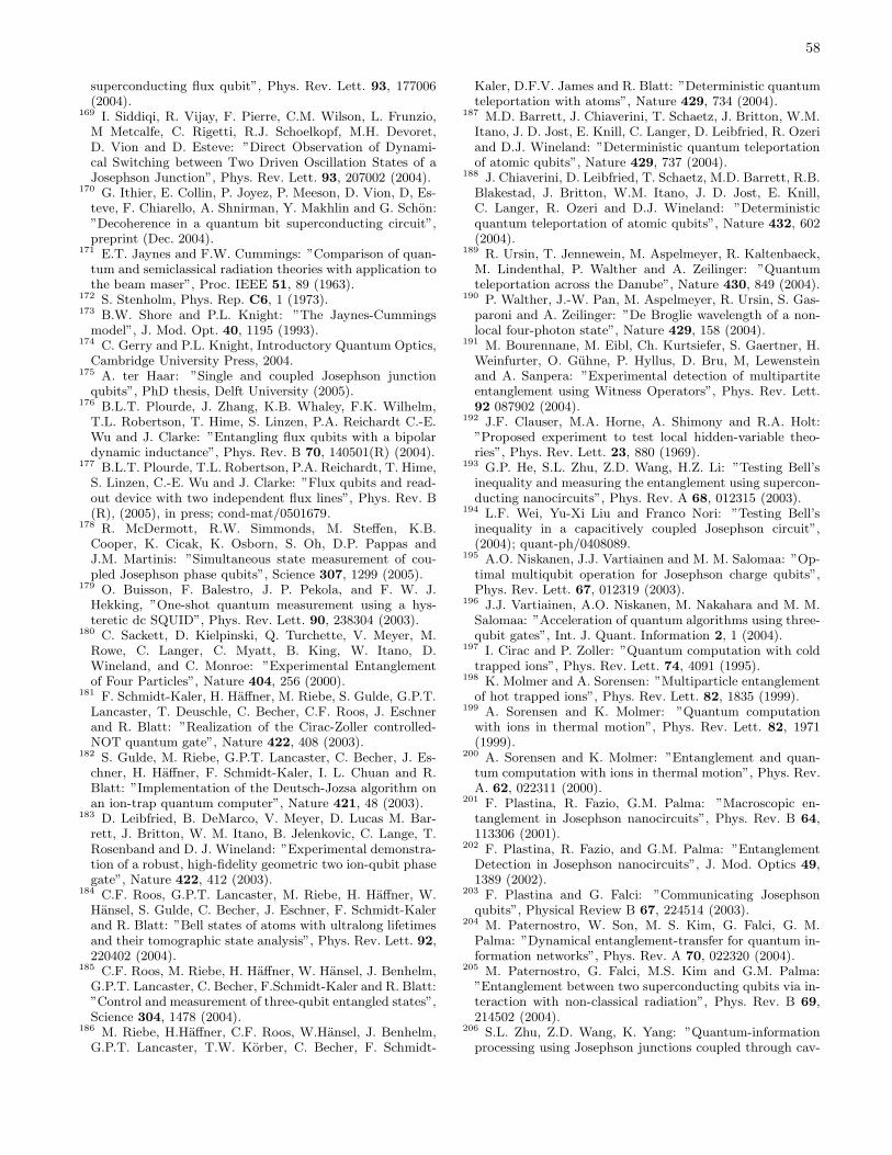
58

superconducting flux qubit”, Phys. Rev. Lett. 93, 177006(2004).

169 I. Siddiqi, R. Vijay, F. Pierre, C.M. Wilson, L. Frunzio,M Metcalfe, C. Rigetti, R.J. Schoelkopf, M.H. Devoret,D. Vion and D. Esteve: ”Direct Observation of Dynami-cal Switching between Two Driven Oscillation States of aJosephson Junction”, Phys. Rev. Lett. 93, 207002 (2004).

170 G. Ithier, E. Collin, P. Joyez, P. Meeson, D. Vion, D, Es-teve, F. Chiarello, A. Shnirman, Y. Makhlin and G. Schon:”Decoherence in a quantum bit superconducting circuit”,preprint (Dec. 2004).

171 E.T. Jaynes and F.W. Cummings: ”Comparison of quan-tum and semiclassical radiation theories with application tothe beam maser”, Proc. IEEE 51, 89 (1963).

172 S. Stenholm, Phys. Rep. C6, 1 (1973).173 B.W. Shore and P.L. Knight: ”The Jaynes-Cummings

model”, J. Mod. Opt. 40, 1195 (1993).174 C. Gerry and P.L. Knight, Introductory Quantum Optics,

Cambridge University Press, 2004.175 A. ter Haar: ”Single and coupled Josephson junction

qubits”, PhD thesis, Delft University (2005).176 B.L.T. Plourde, J. Zhang, K.B. Whaley, F.K. Wilhelm,

T.L. Robertson, T. Hime, S. Linzen, P.A. Reichardt C.-E.Wu and J. Clarke: ”Entangling flux qubits with a bipolardynamic inductance”, Phys. Rev. B 70, 140501(R) (2004).

177 B.L.T. Plourde, T.L. Robertson, P.A. Reichardt, T. Hime,S. Linzen, C.-E. Wu and J. Clarke: ”Flux qubits and read-out device with two independent flux lines”, Phys. Rev. B(R), (2005), in press; cond-mat/0501679.

178 R. McDermott, R.W. Simmonds, M. Steffen, K.B.Cooper, K. Cicak, K. Osborn, S. Oh, D.P. Pappas andJ.M. Martinis: ”Simultaneous state measurement of cou-pled Josephson phase qubits”, Science 307, 1299 (2005).

179 O. Buisson, F. Balestro, J. P. Pekola, and F. W. J.Hekking, ”One-shot quantum measurement using a hys-teretic dc SQUID”, Phys. Rev. Lett. 90, 238304 (2003).

180 C. Sackett, D. Kielpinski, Q. Turchette, V. Meyer, M.Rowe, C. Langer, C. Myatt, B. King, W. Itano, D.Wineland, and C. Monroe: ”Experimental Entanglementof Four Particles”, Nature 404, 256 (2000).

181 F. Schmidt-Kaler, H. Haffner, M. Riebe, S. Gulde, G.P.T.Lancaster, T. Deuschle, C. Becher, C.F. Roos, J. Eschnerand R. Blatt: ”Realization of the Cirac-Zoller controlled-NOT quantum gate”, Nature 422, 408 (2003).

182 S. Gulde, M. Riebe, G.P.T. Lancaster, C. Becher, J. Es-chner, H. Haffner, F. Schmidt-Kaler, I. L. Chuan and R.Blatt: ”Implementation of the Deutsch-Jozsa algorithm onan ion-trap quantum computer”, Nature 421, 48 (2003).

183 D. Leibfried, B. DeMarco, V. Meyer, D. Lucas M. Bar-rett, J. Britton, W. M. Itano, B. Jelenkovic, C. Lange, T.Rosenband and D. J. Wineland: ”Experimental demonstra-tion of a robust, high-fidelity geometric two ion-qubit phasegate”, Nature 422, 412 (2003).

184 C.F. Roos, G.P.T. Lancaster, M. Riebe, H. Haffner, W.Hansel, S. Gulde, C. Becher, J. Eschner, F. Schmidt-Kalerand R. Blatt: ”Bell states of atoms with ultralong lifetimesand their tomographic state analysis”, Phys. Rev. Lett. 92,220402 (2004).

185 C.F. Roos, M. Riebe, H. Haffner, W. Hansel, J. Benhelm,G.P.T. Lancaster, C. Becher, F.Schmidt-Kaler and R. Blatt:”Control and measurement of three-qubit entangled states”,Science 304, 1478 (2004).

186 M. Riebe, H.Haffner, C.F. Roos, W.Hansel, J. Benhelm,G.P.T. Lancaster, T.W. Korber, C. Becher, F. Schmidt-

Kaler, D.F.V. James and R. Blatt: ”Deterministic quantumteleportation with atoms”, Nature 429, 734 (2004).

187 M.D. Barrett, J. Chiaverini, T. Schaetz, J. Britton, W.M.Itano, J. D. Jost, E. Knill, C. Langer, D. Leibfried, R. Ozeriand D.J. Wineland: ”Deterministic quantum teleportationof atomic qubits”, Nature 429, 737 (2004).

188 J. Chiaverini, D. Leibfried, T. Schaetz, M.D. Barrett, R.B.Blakestad, J. Britton, W.M. Itano, J. D. Jost, E. Knill,C. Langer, R. Ozeri and D.J. Wineland: ”Deterministicquantum teleportation of atomic qubits”, Nature 432, 602(2004).

189 R. Ursin, T. Jennewein, M. Aspelmeyer, R. Kaltenbaeck,M. Lindenthal, P. Walther and A. Zeilinger: ”Quantumteleportation across the Danube”, Nature 430, 849 (2004).

190 P. Walther, J.-W. Pan, M. Aspelmeyer, R. Ursin, S. Gas-paroni and A. Zeilinger: ”De Broglie wavelength of a non-local four-photon state”, Nature 429, 158 (2004).

191 M. Bourennane, M. Eibl, Ch. Kurtsiefer, S. Gaertner, H.Weinfurter, O. Guhne, P. Hyllus, D. Bru, M, Lewensteinand A. Sanpera: ”Experimental detection of multipartiteentanglement using Witness Operators”, Phys. Rev. Lett.92 087902 (2004).

192 J.F. Clauser, M.A. Horne, A. Shimony and R.A. Holt:”Proposed experiment to test local hidden-variable theo-ries”, Phys. Rev. Lett. 23, 880 (1969).

193 G.P. He, S.L. Zhu, Z.D. Wang, H.Z. Li: ”Testing Bell’sinequality and measuring the entanglement using supercon-ducting nanocircuits”, Phys. Rev. A 68, 012315 (2003).

194 L.F. Wei, Yu-Xi Liu and Franco Nori: ”Testing Bell’sinequality in a capacitively coupled Josephson circuit”,(2004); quant-ph/0408089.

195 A.O. Niskanen, J.J. Vartiainen and M. M. Salomaa: ”Op-timal multiqubit operation for Josephson charge qubits”,Phys. Rev. Lett. 67, 012319 (2003).

196 J.J. Vartiainen, A.O. Niskanen, M. Nakahara and M. M.Salomaa: ”Acceleration of quantum algorithms using three-qubit gates”, Int. J. Quant. Information 2, 1 (2004).

197 I. Cirac and P. Zoller: ”Quantum computation with coldtrapped ions”, Phys. Rev. Lett. 74, 4091 (1995).

198 K. Molmer and A. Sorensen: ”Multiparticle entanglementof hot trapped ions”, Phys. Rev. Lett. 82, 1835 (1999).

199 A. Sorensen and K. Molmer: ”Quantum computationwith ions in thermal motion”, Phys. Rev. Lett. 82, 1971(1999).

200 A. Sorensen and K. Molmer: ”Entanglement and quan-tum computation with ions in thermal motion”, Phys. Rev.A. 62, 022311 (2000).

201 F. Plastina, R. Fazio, G.M. Palma: ”Macroscopic en-tanglement in Josephson nanocircuits”, Phys. Rev. B 64,113306 (2001).

202 F. Plastina, R. Fazio, and G.M. Palma: ”EntanglementDetection in Josephson nanocircuits”, J. Mod. Optics 49,1389 (2002).

203 F. Plastina and G. Falci: ”Communicating Josephsonqubits”, Physical Review B 67, 224514 (2003).

204 M. Paternostro, W. Son, M. S. Kim, G. Falci, G. M.Palma: ”Dynamical entanglement-transfer for quantum in-formation networks”, Phys. Rev. A 70, 022320 (2004).

205 M. Paternostro, G. Falci, M.S. Kim and G.M. Palma:”Entanglement between two superconducting qubits via in-teraction with non-classical radiation”, Phys. Rev. B 69,214502 (2004).

206 S.L. Zhu, Z.D. Wang, K. Yang: ”Quantum-informationprocessing using Josephson junctions coupled through cav-

59

ities”, Phys. Rev. A 68, 034303 (2003).207 J.Q. You and F. Nori: ”Quantum information processing

with superconducting qubits in a microwave field”, Phys.Rev. B 68, 064509 (2003).

208 G. De Chiara, R. Fazio, C. Macchiavello, G. M. Palma:”Entanglement production by quantum error correction inthe presence of correlated environment”, Europhys. Lett.67, 714 (2004).

209 S. Bose: ”Quantum communication through an unmodu-lated spin chain”, Phys. Rev. Lett. 91 207901 (2003).

210 M. Christandl, N. Datta, A. Ekert and A.J. Landahl:”Perfect state transfer in quantum spin networks”, Phys.Rev. Lett. 92, 187902 (2004).

211 M. Christandl, N. Datta, T. Dorlas, A. Ekert, A. Kayand A.J. Landahl: ”Perfect transfer of arbitrary statessinquantum spin networks”, (2004); quant-ph/0411020.

212 C. Albanese, M. Christandl, N. Datta and A. Ekert: ”Mir-ror inversion of quantum states in linear registers”, Phys.Rev. Lett. 93, 230502 (2004).

213 G. De Chiara, R. Fazio, C. Macchiavello, S. Montangero,G. M. Palma: ”Quantum cloning in spin networks”, Phys.Rev. A 70, 062308 (2004).

214 G. De Chiara, R. Fazio, C. Macchiavello, S. Montangero,G.M. Palma: ”Quantum cloning without external control”,(2004); quant-ph/0410211.

215 A. Romito, R. Fazio and C. Bruder: ”Solid-State Quan-tum Communication With Josephson Arrays”, Phys. Rev.B 71, 100501(R) (2005)..

216 S. Montangero, G. Benenti and R. Fazio: ”Dynamics ofentanglement in quantum computers with imperfections”,Phys. Rev. Lett. 91, 187901 (2003).

217 S. Montangero, A. Romito, G. Benenti and R. Fazio:”Chaotic dynamics in superconducting nanocircuits”,(2004); cond-mat/0407274.

218 P. Facchi, S. Montangero, R. Fazio and S. Pascazio: ”Dy-namical imperfections in quantum computers”, Phys. Rev.A, in press; quant-ph/0407098.

219 M. Paternostro, G.M. Palma, M.S. Kim and G.Falci: ”Quantum state transfer in imperfect artifi-cial spin networks”, Phys. Rev. A 71, 042311 (2005);quant-ph/0407058.

220 P.W. Shor: ”Scheme for reducing decoherence in quantumcomputer memory”, Phys. Rev. A 52, R2493 (1995).

221 E. Knill, R. Laflamme, R. Martinez and C. Negrevergne:”Implementation of the five qubit correction benchmark”,Phys. Rev. Lett. 86, 5811 (2001).

222 A.M. Steane: ”Active stabilisation, quantum computa-tion, and quantum state synthesis”, Phys. Rev. Lett. 77,793 (1996).

223 A.M. Steane: ”Active stabilisation, quantum computa-tion, and quantum state synthesis”, Phys. Rev. Lett. 78,2252 (1997).

224 A.M. Steane: ”Quantum computing and error cor-rection”, in Decoherence and its implications in quan-tum computation and information transfer, Gonis andTuchi (eds.), pp.282-298 (IOS Press, Amsterdam, 2001);quant-ph/0304016.

225 A.M. Steane: ”Overhead and noise threshold of fault-tolerant error correction”, Phys. Rev. A 68, 042322 (2003).

226 A.M. Steane: ”Information science: Quantum errors cor-reted”, Nature 432, 560 (2004).

227 M. Sarovar and G.J. Milburn: ”Continuous quantum er-ror correction by cooling”, (2005); quant-ph/0501038.

228 E. Celeghini, L. Faoro, and M. Rasetti: ”Dynamical alge-

bra of single and coupled Josephson Junctions”, Phys. Rev.B 62, 3054 (2000).

229 D.A. Lidar and K.B. Whaley: ”Decoherence-free sub-spaces and subsystems”, in ”Irreversible Quantum Dy-namics”, F. Benatti and R. Floreanini (Eds.), pp. 83-120(Springer Lecture Notes in Physics vol. 622, Berlin, 2003).

230 L. Viola, E. Knill and S. Lloyd: ”Dynamical decoupling ofopen quantum systems”, Phys. Rev. Lett. 82, 2417 (1999).

231 L. Faoro and L. Viola, ”Dynamical suppression of 1/fnoise processes in qubit systems”, Phys. Rev. Lett. 92,117905 (2004).

232 A. Shnirman and Yu. Makhlin: ”Quantum Zeno effect inthe Cooper-pair transport through a double-island Joseph-son system”, JETP Lett. 78, 447 (2003).

233 G. Falci, A. D’Arrigo, A. Mastellone and E. Paladino,”Dynamical suppression of telegraph and 1/f noise due toquantum bistable fluctuator”, Phys. Rev. A 70, R40101(2004).

234 P. Facchi, D.A. Lidar, and S. Pascazio: ”Unification ofdynamical decoupling and the quantum Zeno effect”, Phys.Rev. A 69, 032314 (2004).

235 P. Facchi, S. Tasaki, S. Pascazio, H. Nakazato, A. Tokuse,and D.A. Lidar: ”Control of decoherence: Analysis andcomparison of three different strategies”, Phys. Rev. A 71,022302 (2005).

236 R. Alicki: ”A unified picture of decoherence control”,(2005); quant-ph/0501109.

237 Yu. Makhlin, G. Schon, and A. Shnirman: ”Josephsonjunction quantum logic gates”, Computer Physics Commu-nications (Elsevier) 127, 156 (2000).

238 J. Siewert and R. Fazio: ”Quantum algorithms for Joseph-son networks”, Phys. Rev. Lett. 87, 257905 (2001).

239 N. Schuch, J. Siewert: ”Implementation of the four-bitDeutsch-Jozsa algorithm with Josephson charge qubits”,physica status solidi (b) 233 (3), 482 (2002).

240 J. Siewert and R. Fazio: ”Implementation of the Deutsch-Jozsa algorithm with Josephson charge qubits”, J. Mod.Optics 49, 1245 (2002)

241 N. Schuch and J. Siewert: ”Progammable networks forquantum algorithms”, Phys. Rev. Lett. 91, 027902 (2003).

242 J.J. Vartiainen, A.O. Niskanen, M. Nakahara and M.M.Salomaa: ”Implementing Shor’s algorithm on Josephsoncharge qubits”, Phys. Rev. A 70, 012319 (2004).

243 J. Zhang, J. Vala, S. Sastry and K.B. Whaley: ”Minimumconstruction of two-qubit operations”, Phys. Rev. Lett. 93,020502 (2004).

244 A.O. Niskanen, M. Nakahara and M. M. Salomaa: ”Real-ization of arbitrary gates in holonomic quantum computa-tion”, Phys. Rev. A 90, 197901 (2003).

245 J. Siewert, L. Faoro, R. Fazio: ”Holonomic quantum com-putation with Josephson networks”, phys. stat. sol. 233,490 (2002)

246 G. Falci, R. Fazio and G.M, Palma: ”Quantum gates andBerry phases in Josephson nanostructures”, Fortschritte derPhysik 51, 442 (2003).

247 L. Faoro, J. Siewert and R. Fazio: ”Non-Abelian phases,pumping, and quantum computation with Josephson junc-tions”, Phys. Rev. Lett. 90, 028301 (2003)

248 G. Falci, R. Fazio, G.M. Palma, J. Siewert and V. Vedral:”Detection of geometric phases in superconducting nanocir-cuits”, Nature 407, 355 (2000).

249 M. Cholascinski: ”Quantum holonomies with Josephson-junction devices”, Phys. Rev. A 69, 134516 (2004).

250 Yu. Makhlin and A. Mirlin: ”Counting statistics for ar-

60

bitrary cycles in quantum pumps” Phys. Rev. Lett. 87,276803 (2001).

251 M. Aunola and J. J. Toppari: ”Connecting Berry’s phaseand the pumped charge in a Cooper pair pump”, Phys. Rev.B 68, 020502 (2003).

252 D.V. Averin: ”Adiabatic quantum computation withCooper pairs”, Solid State Commun. 105, 659 (1998).

253 D. Aharonov, W. van Dam, J. Kempe, Z. Landau, S.Lloyd, O. Regev: ”Adiabatic quantum computation is

equivalent to standard quantum computation”, Proc. 45thFOCS (2004), p. 42-51; quant-ph/0405098.

254 A.M. Steane: ”How to build a 300 bit, 1 Gop quantumcomputer”, quant-ph/0412165 (2004).

255 L. Tian, P. Rabl, R. Blatt, and P. Zoller: ”Interfacingquantum-optical and solid-state qubits”, Phys. Rev. Lett.92, 247902 (2004).