DEPARTMENT OF ECONOMICS - Faculty of Business and Economics

ISSN 0819-2642 ISBN 0 7340 2580 7

THE UNIVERSITY OF MELBOURNE

DEPARTMENT OF ECONOMICS

RESEARCH PAPER NUMBER 924

DECEMBER 2004

TESTING FOR A LEVEL EFFECT IN SHORT-TERM INTEREST RATES

by

Olan T. Henry &

Sandy Suardi

Department of Economics The University of Melbourne Melbourne Victoria 3010 Australia.

Testing for a Level Effect in Short-TermInterest Rates∗

Ólan T. Henry†and Sandy SuardiDepartment of Economics, The University of Melbourne

This version: 10th December 2004

Abstract

There is an extensive theoretical and empirical literature discussingthe link between short-term interest rate volatility and interest ratelevels. We present an LM based test for the presence of a level effectwhich is robust to the presence of unidentified nuisance parameterunder the null of no level effect. We provide extensive Monte-Carloevidence on the performance of this test under various DGPs. Whenapplied to data on the 3-month US Treasury Bills rate, the test reportssignificant evidence of a level effect.

Keywords: Level Effects; LM Tests; Davies ProblemJ.E.L. Reference Numbers: C12; G12; E44

∗Discussions with Nilss Olekalns, Chris Skeels and Kalvinder Shields greatly assistedthe development of this paper. We are grateful to the ARC for financial support un-der Discovery Grant Number DP0451719. Any remaining errors or ommissions are theresponsibility of the authors.

†Corresponding author: Department of Economics, The University of Melbourne, Vic-toria 3010, Australia. E-Mail: [email protected]. Tel: + 61 3 9344 5312. Fax: + 61 39344 6899

1

1 Introduction

Single factor models of the term structure of interest rates imply that allrates move in the same direction over any short time interval. This theoreticalapproach to modelling the term structure of interest rates assumes a plausibleprocess for the short term interest rate that governs the dynamics of theentire term structure. In the empirical literature on short term interest ratesthere is strong evidence that the volatility of short-term interest rates ispositively correlated with the level of the short term rate of interest. Thistendency for interest rates to be more volatile as short term rates rise iscommonly referred to as the level effect. The parameterisation of recenttheoretical and empirical models of the term structure of interest rate reflectthe importance of the level effect in constructing an adequate conditionalcharacterisation of the dynamics of the short term rate of interest. Dothan(1978), Brennan and Schwartz (1977, 1980) add Cox, Ingersoll and Ross(1985), inter alia, all specify the volatility of short-term interest rates as afunction of short-rate levels. Empirical models of the short rate estimated byChan, Karolyi, Longstaff and Sanders (1992), Brenner, Harjes and Kroner(1996), Dewachter (1996), and Koedijk et al. (1997), inter alia also reporteda strongly significant dependence in the short rate volatility on short-ratelevels.Despite the apparent importance of the level effect, as yet no method has

been developed to specifically detect the dependence of short rate volatilityon short-rate levels. The main difficulty in testing for the null of no levelseffect arises from the potential presence of an unidentified nuisance para-meter under the null hypothesis. As a result, the current practice solelyrelies on post-modelling misspecification tests to evaluate the adequacy ofthe model. Brenner et al. (1996), for example, use the conditional momenttest of Woodridge (1990) to test for model misspecification associated with alevel effect. Koedijk et al. (1997) employ a Lagrange multiplier misspecifica-tion test from Wooldridge (1994) and Bollerslev and Wooldridge (1992) thatis robust to deviations from normality in the data. In testing for the presenceof a level effect these authors all assume a specific value for the unidentifiedexponent parameter associated with the lagged interest rate level. However,given that the true value of the exponent parameter is not known a pri-ori, this approach may lead to invalid inference when the true value of theexponent parameter differs from the assumed value.This paper presents a test for the presence of a level effect that is ro-

bust to the presence of an unidentified nuisance parameter under the nullhypothesis. The test is based on the Lagrange multiplier principle and fol-lows the approach for testing for the null of linearity against the alternative

2

of a smooth transition autoregressive (STAR) model discussed in Luukonnenet al. (1988). Under the null hypothesis of no level effect, the problems as-sociated with an unidentified nuisance parameter are overcome by taking aTaylor series approximation around the nuisance parameter. The test, there-fore, has the advantage of not requiring the practitioner to assume any knownvalue for the actual value of the exponent parameter of the interest rate level.In addition, the level effect test statistic is shown to be approximately dis-tributed as a Chi-square variate with one or two degrees of freedom underthe null hypothesis of no level effect.A series of Monte Carlo experiments suggest that the test is largely free

from size distortions and has desirable power for the sample sizes typicallyused in studies of short-term interest rate dynamics. The test is also rel-atively robust to variance asymmetry, the degree of persistence in the con-ditional variance, the presence of mean reversion in the short rate and tomultiplicative levels effects.The organization of this paper is as follows. Section 2 discusses the

formulation of the levels effect in short-term interest rates and the developsthe level effect diagnostic test. Section 3 describes the design and conduct ofthe Monte Carlo experiments to study the small and large sample propertiesof the level effect test. This section also discusses sensitivity analyses forneglected asymmetry in volatility, different degrees of persistence in the leveleffect and the conditional variance, and mean reversion in the short-rateprocess. In the fourth section the level effect test is applied to the U.S. three-month Treasury bill data sampled at a weekly frequency and the results areused to aid the development of empirical models of short-term interest ratedynamics. Section 5 summarizes and concludes.

2 Short Rate Models and the Level EffectTest

2.1 Short Rate Models with Level Effects

Chan, Karolyi, Longstaff and Sanders (1992) (CKLS, hereafter) propose thegeneral non-linear process for short-term interest rates, rt, t ≥ 0, writtenas

dr = (µ+ λr) dt+ φrδdW. (1)

Here r represents the level of the short-term interest rate, W is a Brownianmotion and µ, λ and δ are parameters. The drift component of short-terminterest rates is captured by µ+λr while the variance of unexpected changes

3

in interest rates equals φ2r2δ. The parameter φ is a scale factor and δ controlsthe degree to which the interest rate level influences the volatility of short-term interest rates. By placing restrictions on δ, the Chan et al. (1992)model nests many of the existing interest rate models. For example, whenδ = 0 then (1) reduces to the Vasicek (1977) model, while δ = 1/2 yields theCox, Ingersoll and Ross (1985) model, see Chan et al. (1992) inter alia forfurther details.Brenner, Harjes and Kroner (1996) (BHK, hereafter) argue that by al-

lowing φ2 to be a time varying function of the information set, Ω, it gives riseto a superior conditional characterisation of short term interest rate changes.CKLS and BHK, inter alia, consider the Euler-Maruyama discrete time ap-proximation to (1) written as

∆rt = µ+ λrt−1 + εt. (2)

HereΩt−1 represents the information set available at time t−1 andE (εt|Ωt−1) =0. Letting ht represent the conditional variance of the short-term interest ratethen E (ε2t |Ωt−1) ≡ ht = φ2r2δt−1. The sole source of conditional heteroscedas-ticity in (2) is through the level of the interest rate and thus excludes theinformation arrival process.One common approach to capturing the effect of news is the GARCH(1,1)

modelht = α0 + βht−1 + α1ε

2t−1. (3)

The innovation εt represents a change in the information set from time t− 1to t and can be treated as a collective measure of news. In (3) only themagnitude of the innovation is important in determining ht. BHK extend(2) to allow for volatility clustering caused by information arrival using

∆rt = µ+ λrt−1 + εt.

E (εt|Ωt−1) = 0, E¡ε2t |Ωt−1

¢ ≡ ht = φ2t r2δt−1

φ2t = α0 + α1ε2t−1 + βφ2t−1 (4)

Equation (4) defines the multiplicative level effect model given that theconditional volatility of the short-rate chage is multiplicatively dependent onthe short rate levels. In high information periods, when the magnitude of εtis largest then the sensitivity of volatility to the level of short term interestrates is highest. Under the restriction α1 = β = 0, (4) collapses to (2) andvolatility depends on levels alone. Furthermore when δ = 0 then there is nolevels effect. Testing the null of no level effect (i.e. δ = 0) does not pose anyproblem in the multiplicative level effect model.

4

An alternative approach to modelling volatility clustering and levels ef-fects is the additive level effect model

ht = α0 + α1ε2t−1 + βht−1 + brδt−1. (5)

Under the null hypothesis α1 = β = 0, volatility depends on interest ratelevels alone. If b = 0 then there is no levels effect, however under this nullthe parameter δ is unidentified and so tests of the null hypothesis H0 : b = 0will have a non-standard distribution, see Davies (1987) for further details.To accommodate the Davies problem, other authors test the null H0 : b = 0assuming δ is known. For instance Longstaff and Schwartz (1992) and BHK,inter alia, assume δ = 1.0 while Bekaert, Hodrick andMarshall (1997) assumeδ = 0.5.

2.2 The Level Effect Test

To develop a test for the null of no level effect we consider a short-rate modelthat is free from mean reversion:

∆rt = εt

εt|Ωt−1 ∼ N (0, ht)

ht = α0 + α1ε2t−1 + βht−1 + brδt−1. (6)

where β + α1 < 1, and β, αi, b > 0 for i = 0 and 1. There is little empiricalevidence of mean reversion in short term interests rates, see Rose (1988),Shea (1992), Brenner et al. (1996), and Rodrigues and Rubia(2004), interalia. We relax the assumption of no mean reversion in our Monte-Carloexperiments below. The null hypothesis is that there is no level effect. Thisimplies that the short rate follows a GARCH(1,1) process. Our alternativehypothesis is of a GARCH(1,1) with a level effect. These hypotheses may beformulated as follows

H0 : b = 0

H1 : b 6= 0.

If b = 0 then there is no levels effect, however under this null the parame-ter δ is unidentified and so tests of the null hypothesis H0 : b = 0 will have anon-standard distribution, see Davies (1987) for further details. To addressthis problem we linearize (6) . Sequentially substituting for ht−1 in (6) and

5

taking a first order Taylor series expansion about δ∗ yields

ht =t−1Xi=1

βi−1αo +t−1Xi=1

βi−1α1ε2t−i + βt−1h1 +t−1Xi=1

βi−1brδ∗t−i (1− δ∗ ln rt−i)

+t−1Xi=1

βi−1γrδ∗t−i ln rt−i. (7)

The null hypothesis of no level effect is reformulated as H0 : b = γ =0 where γ = bδ. Assuming that the residual εt is conditionally normallydistributed, a Lagrange Multiplier test statistic under the null hypothesis is

1

2

(TXt=1

∙ε2tht− 1¸ ∙1

ht

∂ht∂

¸)0( TXt=1

∙1

ht

∂ht∂

¸ ∙1

ht

∂ht∂

¸0)−1( TXt=1

∙ε2tht− 1¸ ∙1

ht

∂ht∂

¸)(8)

where

∂ht∂ 0 =

"t−1Xi=1

βi−1

,t−1Xi=1

βi−1

ε2t−i,t−1Xi=1

βi−1

ht−i,t−1Xi=1

βi−1

rδ∗t−i(1− δ∗ ln rt−i),

t−1Xi=1

βi−1

rδ∗t−i ln rt−i

#,

(9)ht is the conditional variance under the null of GARCH(1,1), 0 is the vectorof parameters (α0, α1, β, b, γ), and β is the estimated parameter β in theGARCH(1,1) model. The LM test statistic (8) is asymptotically equivalentto T ·R2 from the outer product auxiliary regression of∙

ε2tht− 1¸

on Xt where

X 0t =

1

ht

⎡⎢⎢⎢⎢⎢⎢⎣

Pt−1i=1 β

i−1Pt−1i=1 β

i−1ε2t−iPt−1

i=1 βi−1

ht−iPt−1i=1 β

i−1rδ∗t−i(1− δ∗ ln rt−i)Pt−1

i=1 βi−1

rδ∗t−i ln rt−i

⎤⎥⎥⎥⎥⎥⎥⎦ . (10)

Here T is the sample size and R2 is the coefficient of determination fromthe regression (10). We refer to this test statistic as LM(δ∗) since it iscomputed using a set of values derived from theoretical short rate models

6

for δ∗ = 0, 0.5, 1, 1.51. The test is approximately distributed as a Chi-square with two degrees of freedom for δ∗ = 0.5, 1, 1.5 although we providesimulated critical values to allow for the approximation error 2.Preliminary Monte Carlo experiments reveal that the empirical size of

LM(δ∗) is significantly larger than the nominal size. This size distortionmay result from a violation of the usual orthogonality conditions. Thenormalized residuals, υt ≡ εt/

√ht, should be orthogonal to

1

ht

"t−1Xi=1

βi−1

,t−1Xi=1

βi−1

ε2t−i,t−1Xi=1

βi−1

ht−i

#, (11)

yet in practice exact orthogonality may not always hold because of the highlynonlinear structure of the model. In the event that these orthogonality con-ditions fail to hold, the empirical size of the test statistic may be distorted(see Engle and Ng , 1993, pp.1759). To correct for the apparent upwardbias in the empirical size of the test statistic, we employ the method intro-duced by Eitrheim and Teräsvirta (1996) and Engle and Ng (1993, pp. 1759).The procedure involves replacing υt with a variable that is guaranteed to beorthogonal to (11). This is done by:

1. Regressing ∙ε2tht− 1¸

on (11). The residuals from this regression, etTt=1, will, by construction,be orthogonal to (11).

2. Then regress et on Xt specified in equation (10) and compute the re-gression R2. The test statistic which is labelled LM1(δ

∗) is set equalto T · R2 and is approximately distributed as a Chi-square with twodegrees of freedom.

1The choice of δ∗ = 0.5, 1.0, 1.5 arises from theoretical short rate models. Whenδ∗ = 0.5, the conditional variance is similar to the square root (SR) process that ap-pears in Cox, Ingersoll and Ross (CIR) (1985) single-factor general equilibrium termstructure model. For δ∗ = 1.0, the model conditional variance then resembles thatof Dothan’s (1978) model, the Geometric Brownian Motion process of Black and Sc-holes (1973), and Brennan and Schwartz (1980) model. While for δ∗ = 1.5, the condi-tional variance is equivalent to the model that CIR (1980) used to study variable rate(VR) securities. We also consider δ∗ = 0 because it simplifies ∂ht

∂ 0 in equation (9) tohPt−1i=1 β

i−1,Pt−1

i=1 βi−1

ε2t−i,Pt−1

i=1 βi−1

ht−i,Pt−1

i=1 βi−1

ln rt−ii.

2In the case of δ∗ = 0, the fourth regressorPt−1

i=1 βi−1

rδ∗t−i(1−δ∗ ln rt−i) in X 0

t simplifies

toPt−1

i=1 βi−1

which is exactly identical to the first regressorPt−1

i=1 βi−1, hence either one

of the regressors may be dropped. In this case the test statistic would be approximatelydistributed as a Chi-square with one degree of freedom.

7

3 A Monte Carlo Experiment

3.1 The Simulated Size of the Test Statistic

To study the simulated size of the level effect test statistic, we generate datafrom the simple GARCH(1,1) process

∆rt = εt , εt =pht · vt where vt v i.i.d.N(0, 1) (12)

ht = α0 + α1ε2t−1 + βht−1

We examine the effect of increasing persistence in the conditional varianceon the simulated size of LM(δ∗) and LM1(δ

∗) test statistics. Following Engleand Ng’s (1993) Monte Carlo study, we employ three sets of parameter values:

1. model H (for high persistence), where (α0, β, α1) = (0.01, 0.9, 0.09) andα1 + β = 0.99

2. model M (for medium persistence), where (α0, β, α1) = (0.05, 0.9, 0.05)and α1 + β = 0.95

3. model L (for low persistence), where (α0, β, α1) = (0.2, 0.75, 0.05) andα1 + β = 0.80

To mitigate the effect of start-up values in all the experiments, we discardthe first 500 observations yielding samples of 500, 1000 and 3000 observations,drawn with 10,000 replications. Upon generating the data, we estimate aGARCH(1,1) specification by maximizing the log-likelihood function usingthe Broyden, Fletcher, Goldfarb and Shanno (BFGS)3 algorithm. The leveleffect test is then calculated on the resulting standardised residuals usingthe test statistics LM(δ∗) and LM1(δ

∗) for δ∗ = 0, 0.5, 1.0, 1.5. Becauseof the highly non-linear structure of the models, in a small fraction of thesereplications, the convergence criterion is not satisfied. In such cases, newreplications are added to ensure that there are 10,000 converged replications.To conserve space we report the results for the LM1(δ

∗). We note thatthere is an upward bias in the empirical size of the uncorrected LM(δ∗)test regardless of the degree of persistence in the conditional variance for allsamples. These results are available upon request from the authors.

- Table 1 here -

The results, presented in Table 1, suggest that for all data generating processesthe corrected test, LM1(δ

∗), exhibits some size distortions for small samples

3The BFGS algorithm with numerical derivatives is discussed in Judd (1988, pp. 114).

8

of 500 and 1000 observations. However, for a sample of 3000 observationsthe empirical size of LM1(δ

∗) is close to the nominal size for the parametervalue of δ∗ = 0.5, 1.0 and 1.5. There is evidence that the empirical size ofLM1(δ

∗) marginally decreases with a less persistent conditional variance.

3.2 Sensitivity Analyses for the Simulated Size

To assess the robustness of the level effect test in the presence of a neglectedasymmetric volatility, we perform the following sensitivity analyses. Follow-ing Engle and Ng (1993), two types of asymmetric GARCH processes areconsidered; they are the EGARCH model due to Nelson (1991) and the GJRspecification due to Glosten et al. (1993). The specifications are as follows:EGARCH Model

εt =pht · vt where vt v i.i.d.N(0, 1) (13)

log(ht) = −0.23 + 0.9 · log(ht−1) + 0.25 ·£v2t−1 − 0.3 · vt−1

¤GJR Model


ht = 0.005 + 0.7 · ht−1 + 0.28 · [|εt−1|− 0.23 · εt−1]2 .The parameter values used in these Monte-Carlo experiments are taken

from Engle and Ng (1993).

- Table 2 here -

The results in Table 2 suggest that, for a sample of 1000 observations, thelevel effect test statistic is robust in the presence of an EGARCH asymmetry,however this is not true in the case of threshold asymmetry of the GJR type.Nevertheless, for the larger sample size there is no apparent distortion inthe empirical size of LM1(δ

∗). This suggests that the empirical size of thetest statistic is robust to EGARCH and GJR asymmetric data generatingprocesses.We also perform sensitivity analyses for the level effect test when the data

generating process displays means reversion using:

∆rt = −0.01rt−1 + εt , εt =pht · vt where vt v i.i.d.N(0, 1) (15)

ht = α0 + α1ε2t−1 + βht−1.

Here the speed of short-rate mean reversion is governed by the value 0.01which is commonly cited in the empirical short-rate models of CKLS and

9

BHK, inter alia. The experiment was performed for a sample of 3000 ob-servations.

- Table 3 here -

Table 3 reports the empirical size of the test statistic for the stationary datagenerating process. The results suggest a minor upward bias in the empiricalsize of LM1(δ

∗). The results, however, are indicative that the level effect testis robust to mean-reversion in the data generating process4. There is furtherevidence that the empirical size of the test statistic also declines with a lesspersistent conditional variance.We also consider the effects of both GJR-type asymmetry and stationarity

on the simulated size of the level effect test. The simulated size is unaffectedby the presence of both asymmetry and stationarity. The results are notreported in the paper to conserve space, but they are available upon requestfrom the authors.

3.3 The Simulated Power of the Test Statistic

The next Monte Carlo experiment studies the simulated power of LM1(δ∗).

The data are generated according to

∆rt = εt

εt =pht · υt where υt ∼ i.i.d.N(0, 1)

ht = α0 + α1ε2t−1 + βht−1 + brδt−1. (16)

We examine the effect of increasing persistence in the conditional varianceon the simulated power of LM1(δ

∗) test statistic using the same parametersvalues as in the empirical size of LM1(δ

∗) test. In addition, the simulatedpower is illustrated for differing degrees of persistence in the level effectthrough changing the values of b and δ. The set of parameter values are b =0.01, 0.5, 0.99 and δ = 0, 0.5, 1.0, 1.5. The size-adjusted power resultsacross different degrees of persistence in the conditional variance, for a sample

4One potential explanation for the observed upward bias in the empirical size is thefailure to account for the first order derivative in the conditional variance function withrespect to the mean equation parameter λ. This is pertinent when computing the vector∂ht∂ 0 defined in equation (9). The cause of such bias might be worthy of an investigationin future research to accommodate different degrees of mean-reversion in the short rateprocess. However, given the lack of evidence of mean reversion in actual data (Shea,1992, Rose, 1998 and Mankiw and Miron,1986 inter alia) we leave this agenda for futureresearch.

10

of 3000 observations, are reported in Table 4 using the simulated criticalvalues which are reported in Table 5.

- Table 4 here -

Apart from the case of b = 0.01 and δ = 0.5, across different combinationsof b and δ the test rejects the null hypothesis of no levels effects in at least95% of simulations for each data generating process. The level effect testalso displays significant size adjusted power across all δ∗ values considered.

− Table 5 here −Empirical values, reported in Table 5, are obtained from simulations used

to examine the empirical size of the corrected level effect test statistic. Giventhat these values are relatively close to the relevant χ2(2) variate, the χ2(2)may be a useful approximation to the true distribution of the test, especiallyfor large samples exceeding 1000 observations.

3.4 Sensitivity Analyses for the Simulated Power

The simulated power of the level effect test in the presence of a neglectedasymmetry is computed using the following conditional variance specificationin the DGP (16):EGARCH Model


log(ht) = −0.23 + 0.9 · log(ht−1) + 0.25 ·£v2t−1 − 0.3 · vt−1

¤+ brδt−1

GJR Model


ht = 0.005 + 0.7 · ht−1 + 0.28 · [|εt−1|− 0.23 · εt−1]2 + brδt−1.

Panels A-C of table 6 report the power of LM1(δ∗) for a sample size

of 3000 in the presence of an unparameterised EGARCH specification. Thepower of the test is computed using the three sets of critical values reported inTable 5, corresponding to the different degrees of persistence in the GARCHprocess. The results indicate that the tests display significant power acrossvarious data generating processes However, when b = 0.01, that is when thelevel effect is weakest, the power of the test is substantially reduced. Theresults also suggest that the empirical power of LM1(δ

∗) varies across thevalues of b and δ considered. Holding the value of b constant the powers of

11

the test declines marginally as the value of δ increases. In contrast, with δconstant the test displays increasing power as the value of b increases.

- Table 6 here -

Table 7 reports the empirical power of LM1(δ∗) for a sample size of 3000 in

the presence of a neglected asymmetry in volatility of the GJR type. Withone exception, the results are similar to those presented in Table 6. Theexception occurs when b = 0.01 and the test displays increasing power as themagnitude of δ increases. For instance, consider b = 0.01 and δ = 0.5, inwhich case the power of the test at the 5% significance level for δ∗ = 0.5 is21.68%. By increasing δ to 1.0 and holding all other parameters constant,the power of the test at the same level of significance increases to 99.94%.

- Table 7 here -

We also perform a sensitivity analysis on the empirical power of LM1(δ∗)

when the DGP displays mean reversion. The data rt is generated as follows:

∆rt = −0.01rt−1 + εt , εt =pht · vt where vt v i.i.d.N(0, 1) (19)

ht = α0 + α1ε2t−1 + βht−1 + brδt−1.

Table 8 presents the results for the empirical power of LM1(δ∗) for a

sample size of 3000 observations. The results largely follow those reportedin Table 4. The only noticeable difference occurs for a weakly persistentlevel effect that is when b = 0.01 and δ = 0.5, where there appears to be animprovement in the power of LM1(δ

∗).

- Table 8 here -

In the presence of GJR-type asymmetry and mean reversion, the power ofLM1(δ

∗) improves for the case of a weakly persistent level effect (i.e. forb = 0.01 and δ = 0.5). The remainder of the results are largely consistentwith those reported in Tables 8. These results are again not reported tosave space but they are available from the authors upon request.Finally, we check for the robustness of the test’s empirical power to DGPs

that display (i) a multiplicative level effect, or (ii) a DGP that follows theCKLS model. The data under each type of specification is generated asfollows:

CKLS : ∆rt = εt , εt = vt · rδ/2t−1 where vt v i.i.d.N(0, 1), (20)

12

Multiplicative Levels Effect : ∆rt = εt , εt =pht·vt·rδ/2t−1 where vt v i.i.d.N(0, 1),

(21)ht = α0 + α1ε

2t−1 + βht−1.

The results reported in Table 9 show that LM1(δ∗) has good power even

when the conditional variance of the DGP does not follow a GARCH processbut contains a levels effect of the type documented in the CKLS model.Allowing for mean reversion in the short rate level marginally improves thepower of the test. Tables 10 presents results that suggest that the test haspower against a multiplicative levels effect, with or without mean reversionin the short rate level.

- Table 9 here -

- Table 10 here -

4 Empirical Application

4.1 Data Description and Diagnostic Tests Results

U.S. three-month Treasury bill yields, sampled at a weekly frequency overthe period January 5, 1965 to November 4, 2003 yielding 2027 observations,were obtained from the FRED II database maintained by the Federal ReserveBank of St. Louis.5

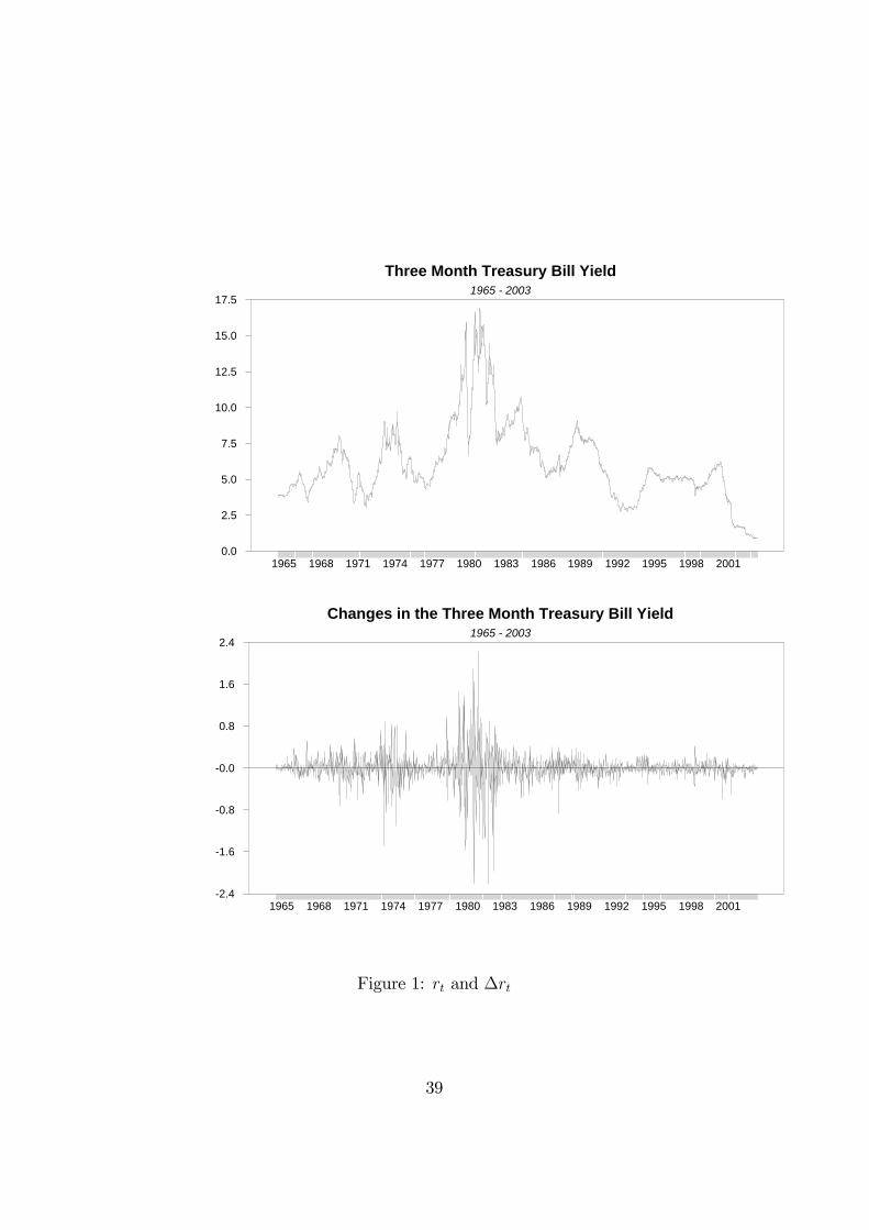
Figure 1 plots the level (rt) and change (∆rt) in the data. Visual in-spection of Figure 1 suggests that the short rate (i) is most volatile betweenthe period of 1979 and 1982 which coincides with the period of change inFederal Reserve monetary policy, (ii) that the volatility of ∆rt increases withthe level of the short rate and (iii) that ∆rt displays volatility clustering.

- Figure 1 here -

Table 11 presents summary statistics for the data series. There is strongevidence of a unit root in the levels rt. However, the change in short rateappears stationary. ∆rt display strong evidence of excess kurtosis. The BeraJarque (1982) test for the normality of ∆rt is significant. Engle’s (1982) LMtest for ARCH, performed using the squared residuals from a fifth orderautoregression provides strong evidence of conditional heteroskedasticity in∆rt. The LM1 (δ

∗) test for a level effect suggests that there is strong evidencethat the volatility of ∆rt is dependent on the lagged short rate level. Engle

5http://research.stlouisfed.org/fred2/

13

and Ng (1993) sign and size bias tests suggest that there is no statisticalevidence supporting asymmetric volatility in the short rate change.

- Table 11 here -

The results from the diagnostic tests suggest that an appropriate empir-ical model of the U.S. short-term interest rate should capture the character-istics of volatility clustering and a levels effect. We start with the estimationof the CKLS short rate specification. In the CKLS model the conditionalheteroscedasticity depends on the lagged short rate level alone. This model,however, fails to specify the news arrival process that may be necessary togenerate the volatility clustering usually associated with short-term inter-est rates. Nonetheless, the CKLS model provides a useful benchmark forthe purpose of comparing with short rate models that explicity account forboth the level effects and the news arrival process. The CKLS discrete-timeeconometric specification of the short rate is

rt − rt−1 = µ+ λrt−1 + ϕCRASH + εt

E(εt) = 0, E(ε2t ) = brδt−1. (22)

The model is estimated using the Generalised Method of Moments (GMM)technique of Hansen (1982).The parameter estimates of CKLS model are reported in column one of

Table 12. The coefficients µ and λ are not significantly different from zeroat conventional levels of significance suggesting that the short rate does notdisplay the property of mean reversion. This result, however, has to betreated with caution since under the null of no mean reversion (i.e. λ = 0),rt has a stochastic trend which implies that the estimated t-ratio for λ isbiased. When using the Dickey-Fuller critical values6, the estimate λ is notsignificantly different from zero. The coefficient of the CRASH dummy, ϕ,is significant at the 5% significance level implying that the expected changein the short rate is higher during the stock market crash in 1989. The con-ditional variance also appears to depend on the lagged short rate level. Thecoefficient δ is significant at 1% significance level. Under the null that themodel (22) is true, Hansen’s (1982) J-test for the goodness-of-fit that is Chi-square distributed with one degree of freedom fails to reject the null at allconventional levels of significance. Some care should be taken in evaluatingthe result of the Hansen J-test because the test is sensitive to the numberand choice of instruments used to estimate the model7. Nonetheless, there

6The Dickey-Fuller critical values with intercept are 3.440, 2.866 and 2.569 at 1%, 5%and 10% significance levels.

7In the GMM estimation, our instruments are the CRASH dummy and rt−1.

14

is evidence that the model is misspecified based on the presence of fifth orderserial correlation in both the residuals and the squared residuals.

- Table 12 about here -

We then estimate short rate models that accommodate both the newsarrival process and the short rate levels effect. In addition to capturing alevel effect, the conditional volatility is allowed to respond asymmetricallyto the sign and size of the short rate innovation in the AsyGARCHL model,specified as:

rt − rt−1 = µ+ λrt−1 + ϕCRASH + εt (23)

E(ε2t |Ωt−1) = ht = α0 + α1ε2t−1 + βht−1 + α2η

2t−1 + b (rt−1/10)

δ

where ηt−1 = min(0, εt−1). For completeness, we also estimate the multiplica-tive level effects short rate model that is consistent with the asymmetric timevarying parameter model of BHK. The specification is as follows

rt − rt−1 = µ+ λrt−1 + ϕCRASH + εt

E¡ε2t |Ωt−1

¢ ≡ ht = φ2t (rt−1/10)δ (24)

φ2t = α0 + α1ε2t−1 + βφ2t−1 + α2η

2t−1.

Both models stated in equations (23) and (24) are estimated using quasimaximum likelihood (QML) methods. Bollerslev and Wooldridge (1992) ar-gue that the asymptotic standard errors resulting from QML are robust todepartures from the normality assumption. We report these robust standarderrors in the tables below.Parameter estimates for the short rate models are reported in column two

to six of Table 11. The asymmetric additive levels model (AsyGARCHL)specified in equation (23) nests the Asymmetric GARCHmodel (AsyGARCH),the GARCH model with level effects (GARCHL) and the GARCH model.The asymmetric multiplicative levels model in equation (24) nests the GARCHmodel with multiplicative levels effects. There is no evidence of mean re-version in short term interest rates in any of the models considered, with µand λ being insignificantly different from zero8 and λ having the wrong sign.The coefficient of the CRASH dummy, ϕ, is significant at 5% significancelevel only in the models where the level effect is specified. Interestingly, inthe variance equation, the sum of the GARCH parameters, α1 + β1 is closeto one only in cases where the level effect is not specified in the model. In

8Again, here, one has to be cautious in interpreting the t-test results since under thenull of no mean reversion, rt is non-stationary and the usual t-test does not apply.

15

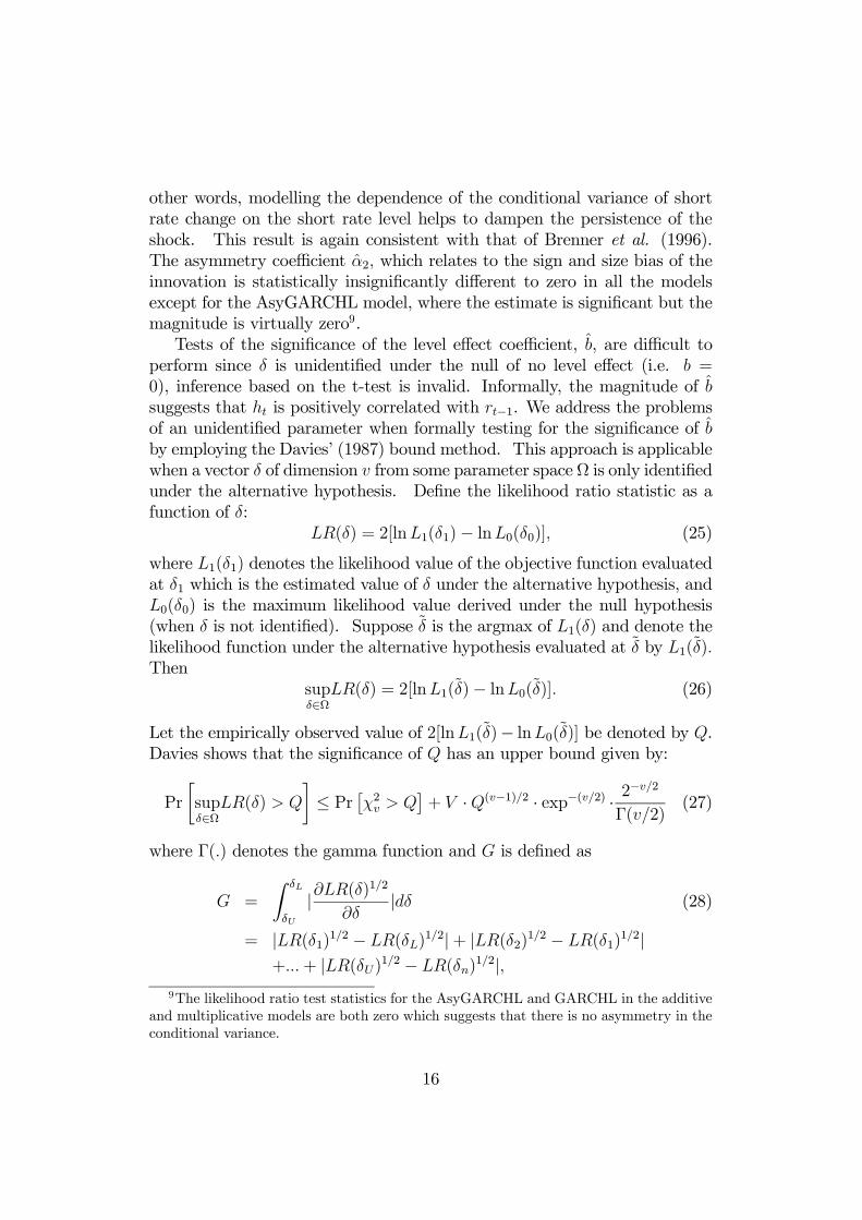
other words, modelling the dependence of the conditional variance of shortrate change on the short rate level helps to dampen the persistence of theshock. This result is again consistent with that of Brenner et al. (1996).The asymmetry coefficient α2, which relates to the sign and size bias of theinnovation is statistically insignificantly different to zero in all the modelsexcept for the AsyGARCHL model, where the estimate is significant but themagnitude is virtually zero9.Tests of the significance of the level effect coefficient, b, are difficult to

perform since δ is unidentified under the null of no level effect (i.e. b =0), inference based on the t-test is invalid. Informally, the magnitude of bsuggests that ht is positively correlated with rt−1. We address the problemsof an unidentified parameter when formally testing for the significance of bby employing the Davies’ (1987) bound method. This approach is applicablewhen a vector δ of dimension v from some parameter space Ω is only identifiedunder the alternative hypothesis. Define the likelihood ratio statistic as afunction of δ:

LR(δ) = 2[lnL1(δ1)− lnL0(δ0)], (25)

where L1(δ1) denotes the likelihood value of the objective function evaluatedat δ1 which is the estimated value of δ under the alternative hypothesis, andL0(δ0) is the maximum likelihood value derived under the null hypothesis(when δ is not identified). Suppose δ is the argmax of L1(δ) and denote thelikelihood function under the alternative hypothesis evaluated at δ by L1(δ).Then

supδ∈Ω

LR(δ) = 2[lnL1(δ)− lnL0(δ)]. (26)

Let the empirically observed value of 2[lnL1(δ)− lnL0(δ)] be denoted by Q.Davies shows that the significance of Q has an upper bound given by:

Pr

∙supδ∈Ω

LR(δ) > Q

¸≤ Pr £χ2v > Q

¤+ V ·Q(v−1)/2 · exp−(v/2) · 2

−v/2

Γ(v/2)(27)

where Γ(.) denotes the gamma function and G is defined as

G =

Z δL

δU

|∂LR(δ)1/2

∂δ|dδ (28)

= |LR(δ1)1/2 − LR(δL)1/2|+ |LR(δ2)1/2 − LR(δ1)

1/2|+...+ |LR(δU)1/2 − LR(δn)

1/2|,9The likelihood ratio test statistics for the AsyGARCHL and GARCHL in the additive

and multiplicative models are both zero which suggests that there is no asymmetry in theconditional variance.

16

where δL, δ1, ..., δn, δU are the turning points of LR(δ). Davies obtained aquick rule by assuming that there is a single peak in the likelihood ratio. Insuch a case, G simplifies to 2Q1/2 which in turn simplifies inequality (27) to

Pr

∙supδ∈Ω

LR(δ) > Q

¸≤ Pr £χ2v > Q

¤+Qv/2 · exp−(v/2) · 2

1−v/2

Γ(v/2). (29)

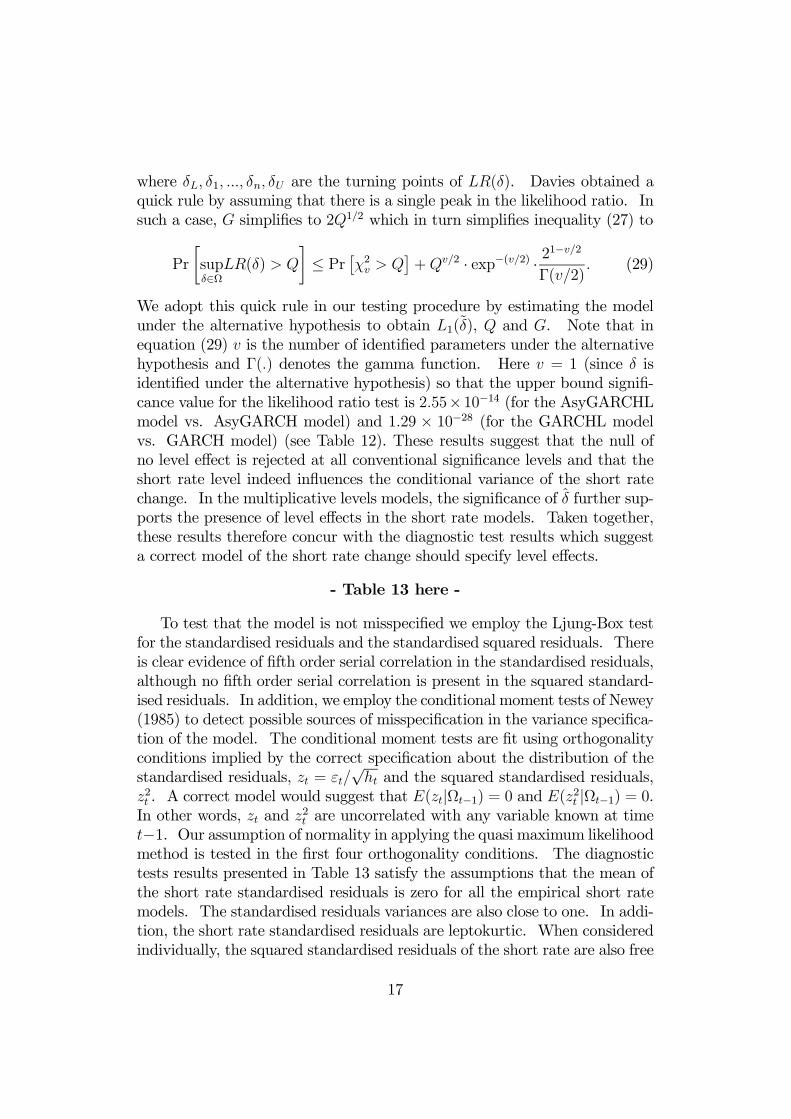
We adopt this quick rule in our testing procedure by estimating the modelunder the alternative hypothesis to obtain L1(δ), Q and G. Note that inequation (29) v is the number of identified parameters under the alternativehypothesis and Γ(.) denotes the gamma function. Here v = 1 (since δ isidentified under the alternative hypothesis) so that the upper bound signifi-cance value for the likelihood ratio test is 2.55×10−14 (for the AsyGARCHLmodel vs. AsyGARCH model) and 1.29 × 10−28 (for the GARCHL modelvs. GARCH model) (see Table 12). These results suggest that the null ofno level effect is rejected at all conventional significance levels and that theshort rate level indeed influences the conditional variance of the short ratechange. In the multiplicative levels models, the significance of δ further sup-ports the presence of level effects in the short rate models. Taken together,these results therefore concur with the diagnostic test results which suggesta correct model of the short rate change should specify level effects.

- Table 13 here -

To test that the model is not misspecified we employ the Ljung-Box testfor the standardised residuals and the standardised squared residuals. Thereis clear evidence of fifth order serial correlation in the standardised residuals,although no fifth order serial correlation is present in the squared standard-ised residuals. In addition, we employ the conditional moment tests of Newey(1985) to detect possible sources of misspecification in the variance specifica-tion of the model. The conditional moment tests are fit using orthogonalityconditions implied by the correct specification about the distribution of thestandardised residuals, zt = εt/

√ht and the squared standardised residuals,

z2t . A correct model would suggest that E(zt|Ωt−1) = 0 and E(z2t |Ωt−1) = 0.In other words, zt and z2t are uncorrelated with any variable known at timet−1. Our assumption of normality in applying the quasi maximum likelihoodmethod is tested in the first four orthogonality conditions. The diagnostictests results presented in Table 13 satisfy the assumptions that the mean ofthe short rate standardised residuals is zero for all the empirical short ratemodels. The standardised residuals variances are also close to one. In addi-tion, the short rate standardised residuals are leptokurtic. When consideredindividually, the squared standardised residuals of the short rate are also free

17

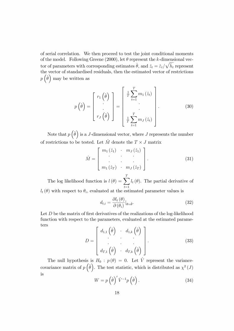
of serial correlation. We then proceed to test the joint conditional momentsof the model. Following Greene (2000), let θ represent the k-dimensional vec-tor of parameters with corresponding estimates θ, and zt = εt/

pht represent

the vector of standardised residuals, then the estimated vector of restrictionsp³θ´may be written as

p³θ´=

⎡⎢⎢⎢⎢⎣r1³θ´

··

rJ³θ´⎤⎥⎥⎥⎥⎦ =

⎡⎢⎢⎢⎢⎢⎢⎢⎢⎣

1T

TXt=1

m1 (zt)

··

1T

TXt=1

mJ (zt)

⎤⎥⎥⎥⎥⎥⎥⎥⎥⎦. (30)

Note that p³θ´is a J-dimensional vector, where J represents the number

of restrictions to be tested. Let M denote the T × J matrix

M =

⎡⎢⎢⎣m1 (z1) · mJ (z1)· · ·· · ·

m1 (zT ) · mJ (zT )

⎤⎥⎥⎦ . (31)

The log likelihood function is l (θ) =TXt=1

lt (θ). The partial derivative of

lt (θ) with respect to θi, evaluated at the estimated parameter values is

dt,i =∂lt (θ)

∂ (θi)|θ=θ. (32)

LetD be the matrix of first derivatives of the realizations of the log-likelihoodfunction with respect to the parameters, evaluated at the estimated parame-ters

D =

⎡⎢⎢⎢⎢⎣d1,1

³θ´· d1,k

³θ´

· · ·· · ·

dT,1³θ´· dT,k

³θ´⎤⎥⎥⎥⎥⎦ . (33)

The null hypothesis is H0 : p (θ) = 0. Let V represent the variance-

covariance matrix of p³θ´. The test statistic, which is distributed as χ2 (J)

isW = p

³θ´0V −1p

³θ´. (34)

18

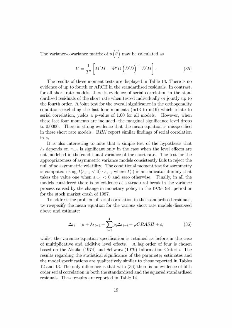
The variance-covariance matrix of p³θ´may be calculated as

V =1

T 2

∙M 0M − M 0D

³D0D

´−1D0M

¸. (35)

The results of these moment tests are displayed in Table 13. There is noevidence of up to fourth or ARCH in the standardised residuals. In contrast,for all short rate models, there is evidence of serial correlation in the stan-dardised residuals of the short rate when tested individually or jointly up tothe fourth order. A joint test for the overall significance in the orthogonalityconditions excluding the last four moments (m13 to m16) which relate toserial correlation, yields a p-value of 1.00 for all models. However, whenthese last four moments are included, the marginal significance level dropsto 0.0000. There is strong evidence that the mean equation is misspecifiedin these short rate models. BHK report similar findings of serial correlationin zt.It is also interesting to note that a simple test of the hypothesis that

ht depends on rt−1 is significant only in the case when the level effects arenot modelled in the conditional variance of the short rate. The test for theappropriateness of asymmetric variance models consistently fails to reject thenull of no asymmetric volatility. The conditional moment test for asymmetryis computed using I(εt−1 < 0) · εt−1 where I(·) is an indicator dummy thattakes the value one when εt−1 < 0 and zero otherwise. Finally, in all themodels considered there is no evidence of a structural break in the varianceprocess caused by the change in monetary policy in the 1979-1981 period orfor the stock market crash of 1987.To address the problem of serial correlation in the standardised residuals,

we re-specify the mean equation for the various short rate models discussedabove and estimate:

∆rt = µ+ λrt−1 +4X

i=1

ρi∆rt−i + ϕCRASH + εt (36)

whilst the variance equation specification is retained as before in the caseof multiplicative and additive level effects. A lag order of four is chosenbased on the Akaike (1974) and Schwarz (1979) Information Criteria. Theresults regarding the statistical significance of the parameter estimates andthe model specifications are qualitatively similar to those reported in Tables12 and 13. The only difference is that with (36) there is no evidence of fifthorder serial correlation in both the standardised and the squared standardisedresiduals. These results are reported in Table 14.

19

-Table 14 here-

On the basis of a series of Likelihood Ratio Tests we are able to reject thehypothesis that the volatility of the US-T Bill rate responds asymetrically topositive and negative shocks. Similarly, we are able to reject the hypothesisthat the levels effect alone is responsible for the conditional heteroscedasticityobserved in ∆rt. Our preferred specifications for ∆rt contain a level effect.We are unable to distinguish between the multiplicative or additive levelseffect models as these models are not nested. It is unclear what effect anunidentified parameter under the null would have on the performance of anon-nested test designed to distinguish across these models. We leave thismatter on the agenda for future research.

5 Summary and Conclusion

This paper develops a test for the presence of a level effect in short terminterest rates. Under the null hypothesis of no level effect the test, which isbased on the Lagrange multiplier principle, is not operational because of thepotential presence of an unidentified parameter. This problem is overcome byperforming a Taylor’s series approximation around the nuisance parameter.The resulting test statistic is approximately distributed Chi-square with oneor two degrees of freedom under the null hypothesis. Monte-Carlo evidencesuggests that, in a large sample, the test statistic is free from significant sizedistortions. The power of the test appears impressive and is largely robust tothe degree of persistence in the GARCH process as well as the strength of thelevels effect. Moreover, the empirical size and power of the test appear to berobust to unparameterised asymmetry in volatility when the levels effect ishighly persistent10. The test also has good power in detecting the presenceof a level effect when the DGP contains either a multiplicative levels effector follows the CKLS model.One caveat of the test is its low power whensubjected to an EGARCH asymmetry and a weak levels effect.A series of Monte Carlo experiments show that the performance of the

level effect test is largely unaffected by the presence of mean-reversion inthe data generating process. The empirical size of the level effect test alsolittle if any distortion if the data generating process displays both asymmetryand mean reversion. This is important since there is scant evidence of meanreversion in the literature modelling short-term interest rate dynamicss.10In view of relatively poor power of LM1(δ

∗) when there is neglected asymmetry andweakly levels effect, Henry, Olekalns and Suardi (2004) develop a joint test for both levelseffect and asymmetry.

20

There are limitations to the level effect test developed in this paper. Thetest results are reasonably reliable for a large sample of 3000 observationsor more. The test is also developed under the assumption of normality, yetmany financial series violate the normality condition and are leptokurtic indistribution. In such cases, the performance of the level effect test may besubjected to distortions. Hence future work will consider robustifying thetest under deviations from normality.Finally, both the level effect test and the Engle and Ng (1993) tests

for asymmetry in volatility were applied to a sample of three-month U.S.Treasury bill yields. While the Engle and Ng (1993) tests fail to detect thepresence of asymmetric volatility in the short rate, the LM1 (δ

∗) test providesevidence of a level effect.Asymmetric GARCHmodels with additive and multiplicative level effects

are estimated and the results concur with those of the diagnostics. Inferenceabout the presence of a levels effect, based on Davies’ (1987) bound test whichovercomes the problem of an unidentified parameter under the null, confirmsthe evidence of a level effect. There is little evidence of asymmetry. Thereis no statistical evidence supporting mean-reversion in the U.S. short rate.Similarly there is no evidence of structural instability due to the change inFederal Reserve operating procedures over the period October 1979-October1982.

21

References

[1] Akaike, H. (1974), ‘A new look at statistical model identification’, IEEETranscations an Automatic Control, AC-19, 716-723.

[2] Bekaert, G., R. J. Hodrick and D.A. Marshall (1997), ‘Peso problem:explanations for term structure anomalies’, NBER Working Paper No.W6147.

[3] Bera, A. and C. Jarque (1981), ‘Model specification tests: A simultane-ous approach’, Journal of Econometrics, 20, 59-82.

[4] Black, F. and M. Scholes (1973), ‘The Pricing of Options and CorporateLiabilities’, Journal of Political Economy, 81, 637-654.

[5] Brennan, M.J. and E.S. Schwartz (1980), ‘Analysing Convertible Bonds’,Journal of Financial and Quantitative Analysis, 15, 907-929.

[6] Brenner R.J., R.H. Harjes and K.F. Kroner (1996), ‘Another Look atModels of the Short-term Interest Rate’, Journal of Financial and Quan-titative Analysis, 31, 85-107.

[7] Bollerslev, T. and J.M. Wooldridge (1992), ‘Quasi maximum likelihoodestimation and inference in dynamic models with time varying covari-ances’, Econometric Reviews, 11, 143-172.

[8] Chan, K.C., G.A. Karolyi, F.A. Longstaff and A.B. Sanders (1992), ‘Anempirical comparison of alternative models of the short-term interestrate’, Journal of Finance, 47, 1209-1227.

[9] Cox, John C., J. E. Ingersoll and S.A. Ross (1980), ‘An Analysis ofVariable Rate of Loan Contracts’, Journal of Finance, 35, 389-403.

[10] Cox, John C., J. E. Ingersoll and S.A. Ross (1985), ‘A Theory of theTerm Structure of Interest Rates’, Econometrica, 53, 385-407.

[11] Davies, R.B. (1987), ‘Hypothesis testing when a nuisance parameter ispresent only under the alternative’, Biometrika, 74, 33-43.

[12] Dewachter (1996), ‘Modelling interest rate volatility: Regime switchesand level links’, Weltwirtschaftliches Archiv-Review of World Eco-nomics, 132(2), 236 - 258.

[13] Dothan, U. (1978), ‘On the term structure of interest rates’, Journal ofFinancial Economics, 6, 59-69.

22

[14] Eitrheim, O. and T., Teräsvirta (1996), ‘Testing the adequacy of smoothtransition autoregressive models’, Journal of Econometrics, 74(1), 59-75.

[15] Engle R.F. (1982), ‘Autoregressive conditional heteroscedasticity withestimates of the variance of U.K. inflation’, Econometrica, 50, 987-1008.

[16] Engle, R.F. and V.K, Ng (1993), ‘Measuring and testing the impact ofnews and volatility’, Journal of Finance, 48, 1749-1778.

[17] Glosten, L.R., R. Jagannathan, and D.E. Runkle (1993), ‘On the relationbetween the expected value and the volatility of the nominal excessreturn on stocks’, Journal of Finance, 48(5), 1779-1801.

[18] Greene, W.H. (2000), Econometric Analysis, Prentice-Hall Inc.

[19] Hansen, B.C. (1982), ‘Large sample properties of Generalised Methodof Moments estimators’, Econometrica, 50,1029-1054.

[20] Henry, Ó. T., N. Olekalns and S. Suardi (2004), ‘Modelling comovementsin equity returns and short-term interest rates: Levels effects and asym-metric volatility dynamics’, University of Melbourne, Working Paper.

[21] Koedijk, K.G., F. Nissen, P.C. Schotman and C.P. Wolff. (1997), ‘Thedynamics of short term interest rate volatility reconsidered’, EuropeanFinance Review, 1, 105-130.

[22] Longstaff, F.A. and E.S.Schwartz (1992), ‘Interest rate volatility andthe term structure: A two factor general equilibrium model’, Journal ofFinance, 47, 1259-1282.

[23] Lukkonen, R., P. Saikkonen and T. Teräsvirta (1988), ‘Testing linearityagainst smooth transition autoregressive models’, Biometrika, 75, 491-499.

[24] Mankiw, G. and J.A. Miron (1986), ‘The changing behaviour of theterm structure of interest rates’, the Quarterly Journal of Economics,101(2), 211-228.

[25] Nelson, D. (1991), ‘Conditional heteroskedasticity in asset returns: Anew approach’, Econometrica, 59(2), 347-370.

[26] Newey, W. (1985), ‘Maximum likelihood specification testing and con-ditional moment tests’, Econometrica, 53, 1047-1070.

23

[27] Rodrigues, A. and A. Rubia (2004), ‘On the small sample propertiesof Dickey Fuller and Maximum Likelihood unit root tests on discrete-sampled short-term interest rates’, Manuscript, Department of FinancialEconomics, University of Alicante.

[28] Rose, A.K. (1988), ‘Is the real interest rate stable?’, Journal of Finance,43, 1095-1112.

[29] Schwarz, G. (1978), ‘Estimating the dimension of a model’, The Annalsof Statistics, 6, 461-464.

[30] Shea, G.S. (1992), ‘Benchmarking the Expectations Hypothesis of theinterest rate term structure: An analysis of cointegration vectors’, Jour-nal of Business and Economic Statistics, 10(3), 347-366.

[31] Vasicek, O. (1977), ‘An equilibrium characterization of the term struc-ture’, Journal of Financial Economics, 5(2), 177-188.

[32] Wooldridge, J.M. (1990), ‘A Unified approach to robust, regression-based specification tests’, Econometric Theory, 6(1), 17-43.

[33] Wooldridge, J.M. (1994), ‘Estimation and inference for dependentprocesses’, in R.F. Engle and D.L. McFadden (eds.), Handbook ofEconometrics, Volume 4, North-Holland, Amsterdam.

24

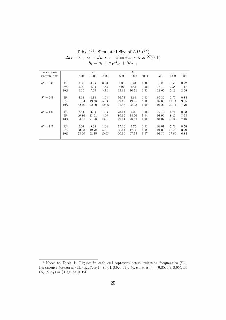
Table 111: Simulated Size of LM1(δ∗)

∆rt = εt , εt =√ht · vt where vt v i.i.d.N(0, 1)

ht = α0 + α1ε2t−1 + βht−1

Persistence H M LSample Size 500 1000 3000 500 1000 3000 500 1000 3000

δ∗ = 0.0 1% 0.00 0.88 0.30 3.05 1.94 0.36 1.45 0.55 0.225% 0.00 4.03 1.88 6.97 6.51 1.60 15.79 2.38 1.1710% 0.20 7.65 3.72 12.68 10.71 3.52 28.65 5.28 2.58

δ∗ = 0.5 1% 4.18 4.16 1.08 56.73 6.61 1.02 62.32 2.77 0.845% 31.84 13.48 5.08 82.68 19.25 5.06 87.63 11.44 3.8510% 52.10 22.09 10.05 91.45 28.93 9.65 94.22 20.14 7.76

δ∗ = 1.0 1% 2.44 3.99 1.06 73.04 6.28 1.00 77.12 1.73 0.635% 49.86 13.21 5.06 89.92 18.76 5.04 91.90 8.42 3.5810% 64.31 21.98 10.01 92.01 28.53 9.68 94.07 16.86 7.18

δ∗ = 1.5 1% 2.64 3.64 1.04 77.16 5.75 1.02 84.01 5.76 0.585% 63.83 12.78 5.01 88.54 17.68 5.02 91.05 17.70 3.2910% 73.29 21.15 10.03 90.90 27.55 9.37 93.30 27.60 6.84

11Notes to Table 1: Figures in each cell represent actual rejection frequencies (%).Persistence Measures - H: (αo, β, α1) =(0.01, 0.9, 0.09), M: αo, β, α1) = (0.05, 0.9, 0.05), L:(αo, β, α1) = (0.2, 0.75, 0.05)

25

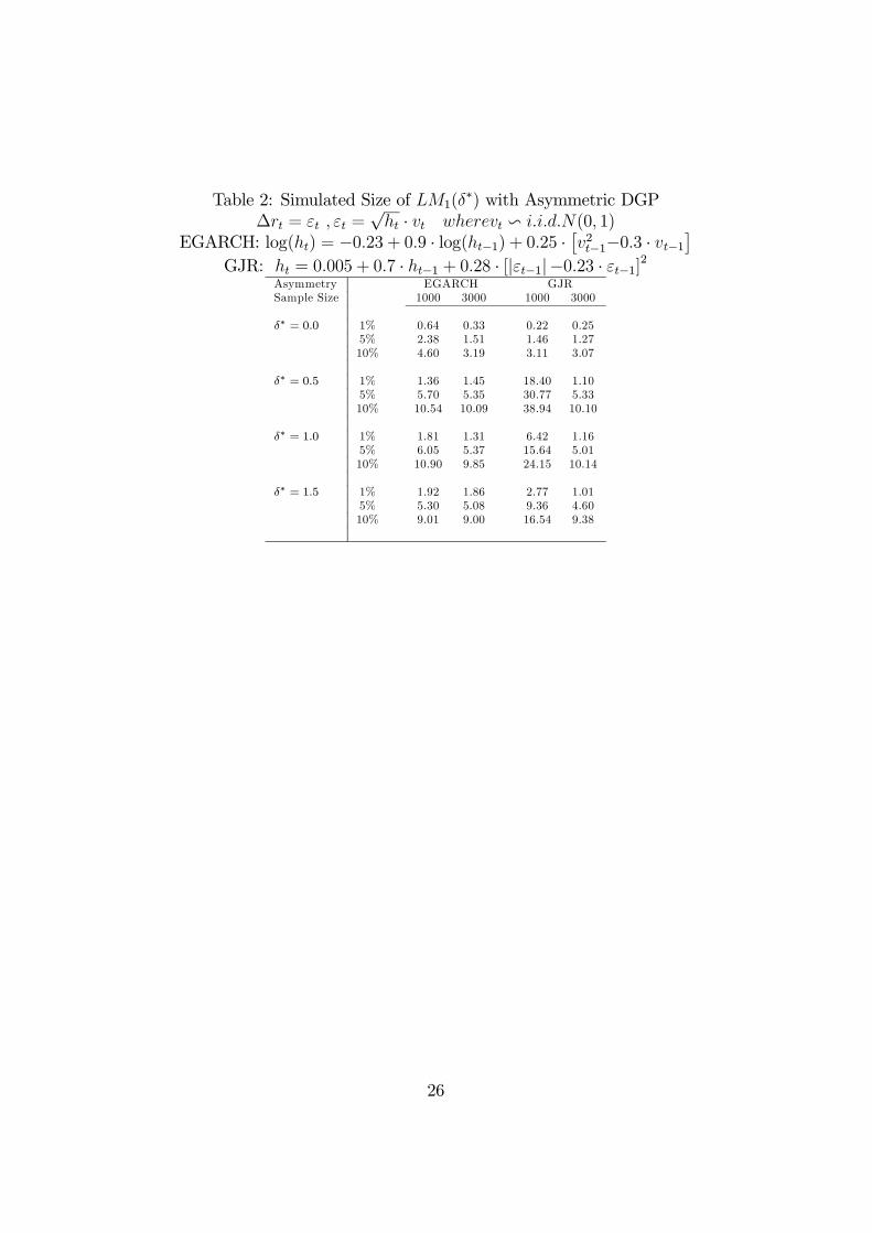
Table 2: Simulated Size of LM1(δ∗) with Asymmetric DGP

∆rt = εt , εt =√ht · vt wherevt v i.i.d.N(0, 1)

EGARCH: log(ht) = −0.23 + 0.9 · log(ht−1) + 0.25 ·£v2t−1−0.3 · vt−1

¤GJR: ht = 0.005 + 0.7 · ht−1 + 0.28 · [|εt−1|−0.23 · εt−1]2

Asymmetry EGARCH GJRSample Size 1000 3000 1000 3000

δ∗ = 0.0 1% 0.64 0.33 0.22 0.255% 2.38 1.51 1.46 1.2710% 4.60 3.19 3.11 3.07

δ∗ = 0.5 1% 1.36 1.45 18.40 1.105% 5.70 5.35 30.77 5.3310% 10.54 10.09 38.94 10.10

δ∗ = 1.0 1% 1.81 1.31 6.42 1.165% 6.05 5.37 15.64 5.0110% 10.90 9.85 24.15 10.14

δ∗ = 1.5 1% 1.92 1.86 2.77 1.015% 5.30 5.08 9.36 4.6010% 9.01 9.00 16.54 9.38

26

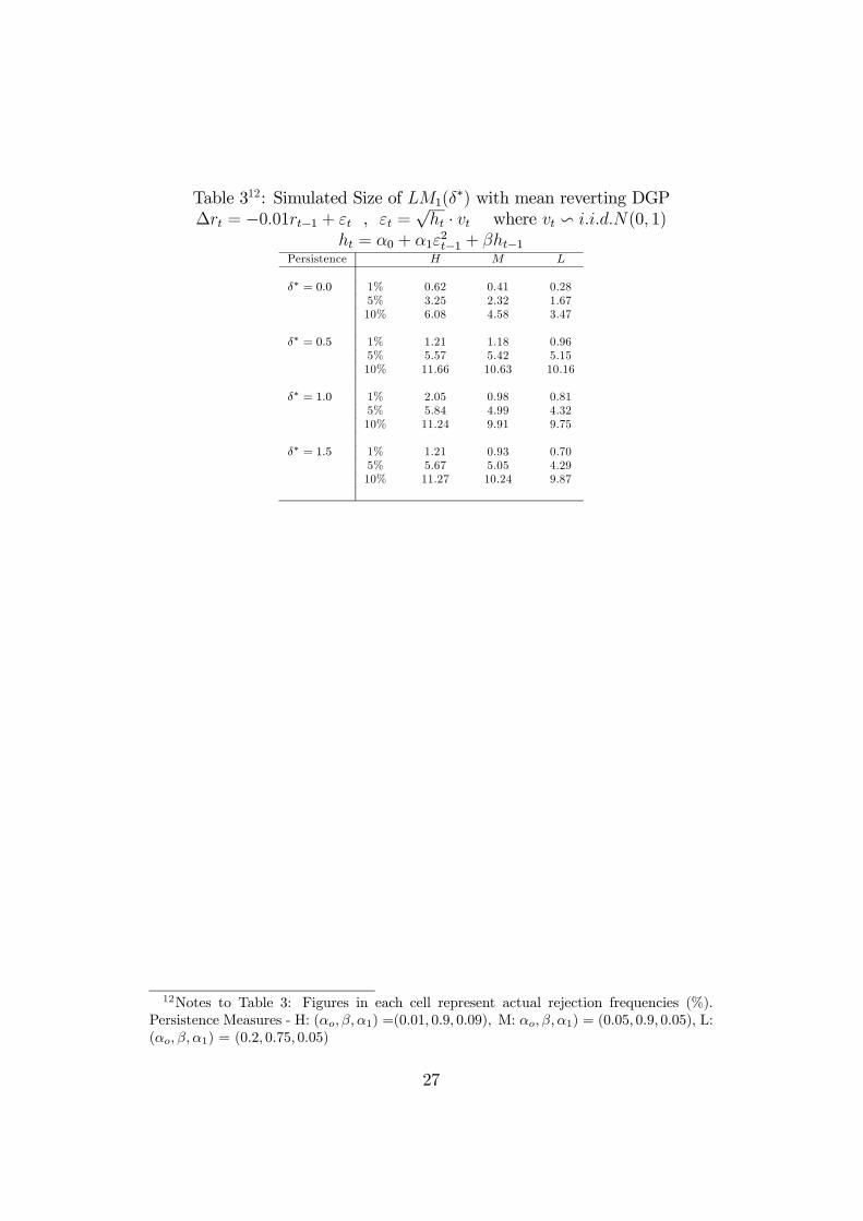
Table 312: Simulated Size of LM1(δ∗) with mean reverting DGP

∆rt = −0.01rt−1 + εt , εt =√ht · vt where vt v i.i.d.N(0, 1)

ht = α0 + α1ε2t−1 + βht−1

Persistence H M L

δ∗ = 0.0 1% 0.62 0.41 0.285% 3.25 2.32 1.6710% 6.08 4.58 3.47

δ∗ = 0.5 1% 1.21 1.18 0.965% 5.57 5.42 5.1510% 11.66 10.63 10.16

δ∗ = 1.0 1% 2.05 0.98 0.815% 5.84 4.99 4.3210% 11.24 9.91 9.75

δ∗ = 1.5 1% 1.21 0.93 0.705% 5.67 5.05 4.2910% 11.27 10.24 9.87


27

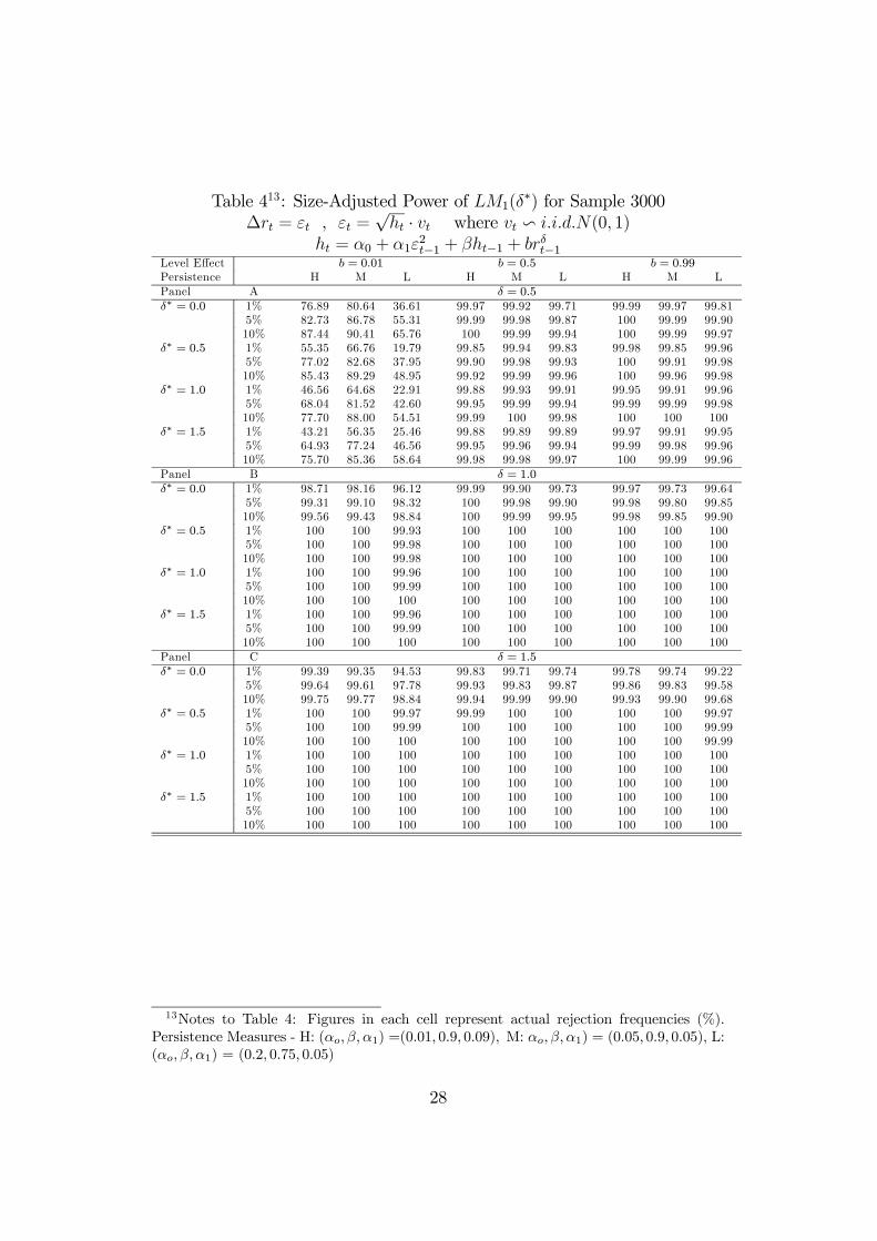
Table 413: Size-Adjusted Power of LM1(δ∗) for Sample 3000

∆rt = εt , εt =√ht · vt where vt v i.i.d.N(0, 1)

ht = α0 + α1ε2t−1 + βht−1 + brδt−1

Level Effect b = 0.01 b = 0.5 b = 0.99Persistence H M L H M L H M LPanel A δ = 0.5δ∗ = 0.0 1% 76.89 80.64 36.61 99.97 99.92 99.71 99.99 99.97 99.81

5% 82.73 86.78 55.31 99.99 99.98 99.87 100 99.99 99.9010% 87.44 90.41 65.76 100 99.99 99.94 100 99.99 99.97

δ∗ = 0.5 1% 55.35 66.76 19.79 99.85 99.94 99.83 99.98 99.85 99.965% 77.02 82.68 37.95 99.90 99.98 99.93 100 99.91 99.9810% 85.43 89.29 48.95 99.92 99.99 99.96 100 99.96 99.98

δ∗ = 1.0 1% 46.56 64.68 22.91 99.88 99.93 99.91 99.95 99.91 99.965% 68.04 81.52 42.60 99.95 99.99 99.94 99.99 99.99 99.9810% 77.70 88.00 54.51 99.99 100 99.98 100 100 100

δ∗ = 1.5 1% 43.21 56.35 25.46 99.88 99.89 99.89 99.97 99.91 99.955% 64.93 77.24 46.56 99.95 99.96 99.94 99.99 99.98 99.9610% 75.70 85.36 58.64 99.98 99.98 99.97 100 99.99 99.96

Panel B δ = 1.0δ∗ = 0.0 1% 98.71 98.16 96.12 99.99 99.90 99.73 99.97 99.73 99.64

5% 99.31 99.10 98.32 100 99.98 99.90 99.98 99.80 99.8510% 99.56 99.43 98.84 100 99.99 99.95 99.98 99.85 99.90

δ∗ = 0.5 1% 100 100 99.93 100 100 100 100 100 1005% 100 100 99.98 100 100 100 100 100 10010% 100 100 99.98 100 100 100 100 100 100

δ∗ = 1.0 1% 100 100 99.96 100 100 100 100 100 1005% 100 100 99.99 100 100 100 100 100 10010% 100 100 100 100 100 100 100 100 100

δ∗ = 1.5 1% 100 100 99.96 100 100 100 100 100 1005% 100 100 99.99 100 100 100 100 100 10010% 100 100 100 100 100 100 100 100 100

Panel C δ = 1.5δ∗ = 0.0 1% 99.39 99.35 94.53 99.83 99.71 99.74 99.78 99.74 99.22

5% 99.64 99.61 97.78 99.93 99.83 99.87 99.86 99.83 99.5810% 99.75 99.77 98.84 99.94 99.99 99.90 99.93 99.90 99.68

δ∗ = 0.5 1% 100 100 99.97 99.99 100 100 100 100 99.975% 100 100 99.99 100 100 100 100 100 99.9910% 100 100 100 100 100 100 100 100 99.99

δ∗ = 1.0 1% 100 100 100 100 100 100 100 100 1005% 100 100 100 100 100 100 100 100 10010% 100 100 100 100 100 100 100 100 100

δ∗ = 1.5 1% 100 100 100 100 100 100 100 100 1005% 100 100 100 100 100 100 100 100 10010% 100 100 100 100 100 100 100 100 100


28

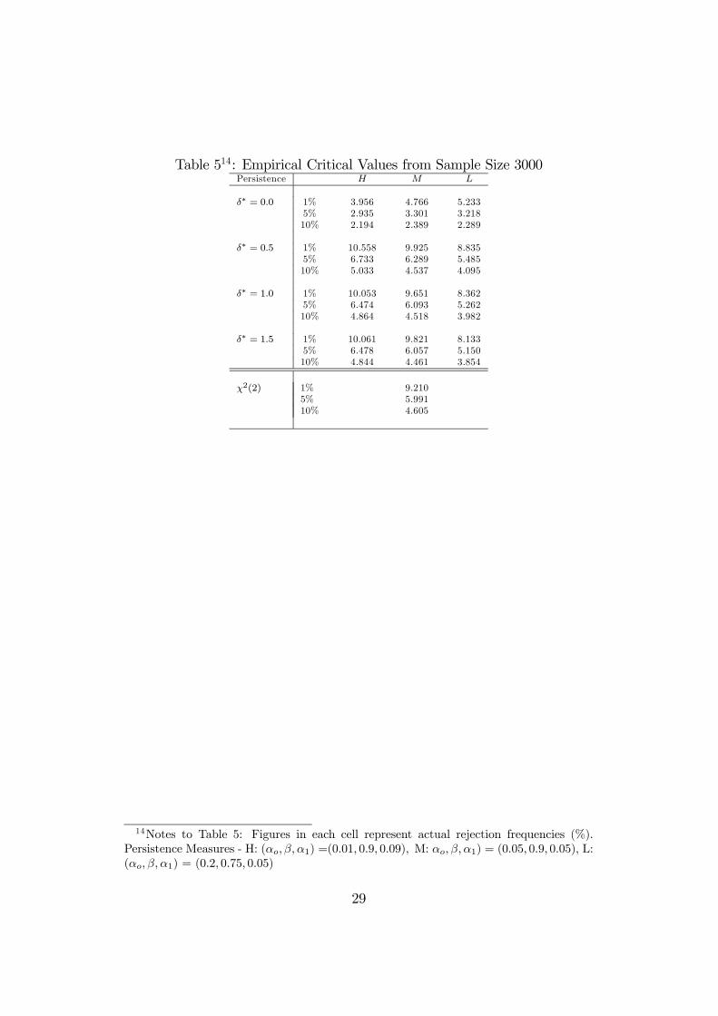
Table 514: Empirical Critical Values from Sample Size 3000Persistence H M L

δ∗ = 0.0 1% 3.956 4.766 5.2335% 2.935 3.301 3.21810% 2.194 2.389 2.289

δ∗ = 0.5 1% 10.558 9.925 8.8355% 6.733 6.289 5.48510% 5.033 4.537 4.095

δ∗ = 1.0 1% 10.053 9.651 8.3625% 6.474 6.093 5.26210% 4.864 4.518 3.982

δ∗ = 1.5 1% 10.061 9.821 8.1335% 6.478 6.057 5.15010% 4.844 4.461 3.854

χ2(2) 1% 9.2105% 5.99110% 4.605


29

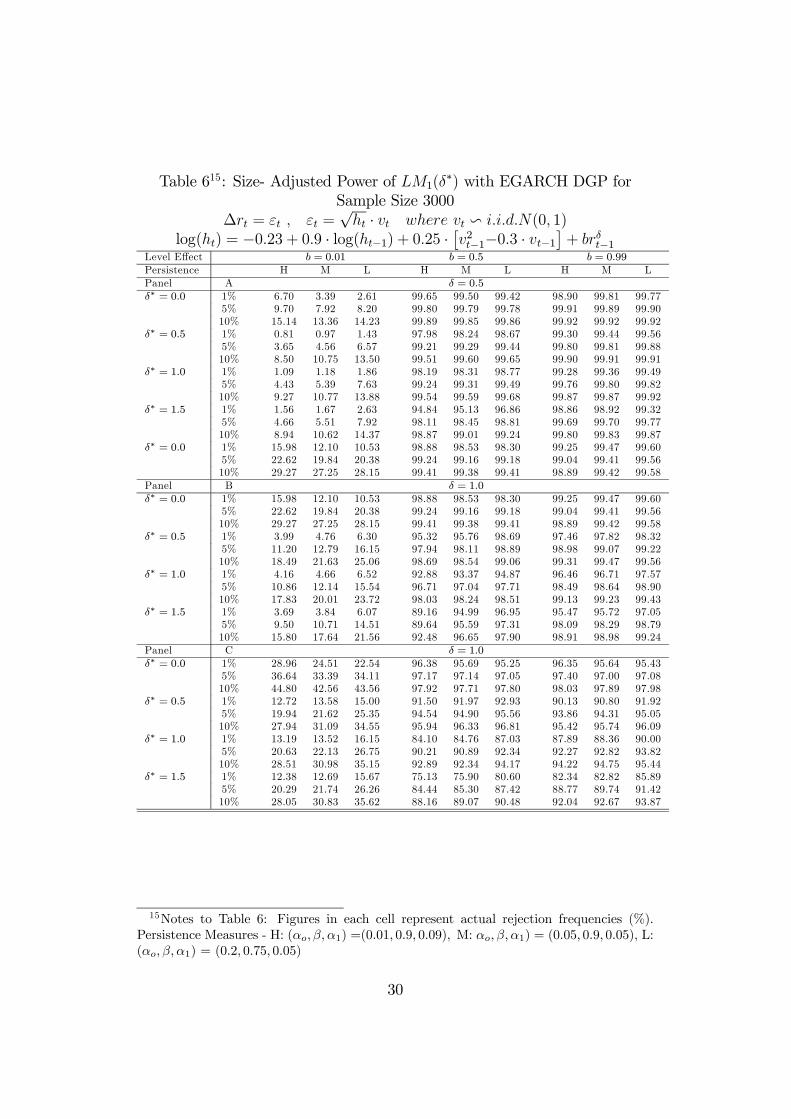
Table 615: Size- Adjusted Power of LM1(δ∗) with EGARCH DGP for

Sample Size 3000∆rt = εt , εt =

√ht · vt where vt v i.i.d.N(0, 1)

log(ht) = −0.23 + 0.9 · log(ht−1) + 0.25 ·£v2t−1−0.3 · vt−1

¤+ brδt−1

Level Effect b = 0.01 b = 0.5 b = 0.99Persistence H M L H M L H M LPanel A δ = 0.5δ∗ = 0.0 1% 6.70 3.39 2.61 99.65 99.50 99.42 98.90 99.81 99.77

5% 9.70 7.92 8.20 99.80 99.79 99.78 99.91 99.89 99.9010% 15.14 13.36 14.23 99.89 99.85 99.86 99.92 99.92 99.92

δ∗ = 0.5 1% 0.81 0.97 1.43 97.98 98.24 98.67 99.30 99.44 99.565% 3.65 4.56 6.57 99.21 99.29 99.44 99.80 99.81 99.8810% 8.50 10.75 13.50 99.51 99.60 99.65 99.90 99.91 99.91

δ∗ = 1.0 1% 1.09 1.18 1.86 98.19 98.31 98.77 99.28 99.36 99.495% 4.43 5.39 7.63 99.24 99.31 99.49 99.76 99.80 99.8210% 9.27 10.77 13.88 99.54 99.59 99.68 99.87 99.87 99.92

δ∗ = 1.5 1% 1.56 1.67 2.63 94.84 95.13 96.86 98.86 98.92 99.325% 4.66 5.51 7.92 98.11 98.45 98.81 99.69 99.70 99.7710% 8.94 10.62 14.37 98.87 99.01 99.24 99.80 99.83 99.87

δ∗ = 0.0 1% 15.98 12.10 10.53 98.88 98.53 98.30 99.25 99.47 99.605% 22.62 19.84 20.38 99.24 99.16 99.18 99.04 99.41 99.5610% 29.27 27.25 28.15 99.41 99.38 99.41 98.89 99.42 99.58

Panel B δ = 1.0δ∗ = 0.0 1% 15.98 12.10 10.53 98.88 98.53 98.30 99.25 99.47 99.60

5% 22.62 19.84 20.38 99.24 99.16 99.18 99.04 99.41 99.5610% 29.27 27.25 28.15 99.41 99.38 99.41 98.89 99.42 99.58

δ∗ = 0.5 1% 3.99 4.76 6.30 95.32 95.76 98.69 97.46 97.82 98.325% 11.20 12.79 16.15 97.94 98.11 98.89 98.98 99.07 99.2210% 18.49 21.63 25.06 98.69 98.54 99.06 99.31 99.47 99.56

δ∗ = 1.0 1% 4.16 4.66 6.52 92.88 93.37 94.87 96.46 96.71 97.575% 10.86 12.14 15.54 96.71 97.04 97.71 98.49 98.64 98.9010% 17.83 20.01 23.72 98.03 98.24 98.51 99.13 99.23 99.43

δ∗ = 1.5 1% 3.69 3.84 6.07 89.16 94.99 96.95 95.47 95.72 97.055% 9.50 10.71 14.51 89.64 95.59 97.31 98.09 98.29 98.7910% 15.80 17.64 21.56 92.48 96.65 97.90 98.91 98.98 99.24

Panel C δ = 1.0δ∗ = 0.0 1% 28.96 24.51 22.54 96.38 95.69 95.25 96.35 95.64 95.43

5% 36.64 33.39 34.11 97.17 97.14 97.05 97.40 97.00 97.0810% 44.80 42.56 43.56 97.92 97.71 97.80 98.03 97.89 97.98

δ∗ = 0.5 1% 12.72 13.58 15.00 91.50 91.97 92.93 90.13 90.80 91.925% 19.94 21.62 25.35 94.54 94.90 95.56 93.86 94.31 95.0510% 27.94 31.09 34.55 95.94 96.33 96.81 95.42 95.74 96.09

δ∗ = 1.0 1% 13.19 13.52 16.15 84.10 84.76 87.03 87.89 88.36 90.005% 20.63 22.13 26.75 90.21 90.89 92.34 92.27 92.82 93.8210% 28.51 30.98 35.15 92.89 92.34 94.17 94.22 94.75 95.44

δ∗ = 1.5 1% 12.38 12.69 15.67 75.13 75.90 80.60 82.34 82.82 85.895% 20.29 21.74 26.26 84.44 85.30 87.42 88.77 89.74 91.4210% 28.05 30.83 35.62 88.16 89.07 90.48 92.04 92.67 93.87


30

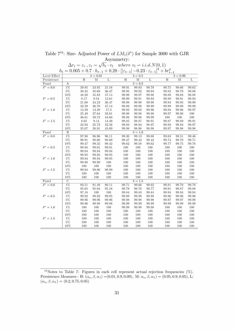
Table 716: Size- Adjusted Power of LM1(δ∗) for Sample 3000 with GJR

Asymmetry:∆rt = εt , εt =


ht = 0.005 + 0.7 · ht−1 + 0.28 · [|εt−1|−0.23 · εt−1]2 + brδt−1Level Effect b = 0.01 b = 0.5 b = 0.99Persistence H M L H M L H M LPanel A δ = 0.5δ∗ = 0.0 1% 29.85 23.92 21.16 99.91 99.83 99.79 99.75 99.66 99.62

5% 39.45 35.69 36.47 99.95 99.92 99.94 99.82 99.79 99.8010% 48.20 45.82 47.14 99.99 99.97 99.98 99.89 99.88 99.88

δ∗ = 0.5 1% 8.17 9.54 12.61 99.99 99.91 99.94 99.89 99.91 99.935% 21.68 24.23 36.47 99.98 99.98 99.98 99.94 99.95 99.9910% 32.59 36.76 47.14 99.98 99.98 99.99 99.99 99.99 99.99

δ∗ = 1.0 1% 12.29 13.39 17.3 99.92 99.92 99.96 99.94 99.96 99.975% 25.49 27.64 33.61 99.98 99.98 99.98 99.97 99.98 10010% 36.61 39.72 44.60 99.98 99.98 99.99 100 100 100

δ∗ = 1.5 1% 8.65 9.14 14.49 99.85 98.87 98.91 99.87 99.89 99.915% 22.93 25.72 32.56 99.93 98.94 98.97 99.93 99.94 99.9710% 35.07 38.91 45.09 99.98 98.98 98.98 99.97 99.98 99.98

Panel B δ = 1.0δ∗ = 0.0 1% 97.98 96.96 96.11 99.30 99.13 99.08 99.63 99.51 99.46

5% 98.91 98.60 98.69 99.47 99.42 99.42 99.74 99.70 99.7110% 99.47 99.32 99.42 99.62 99.58 99.62 99.77 99.75 99.76

δ∗ = 0.5 1% 99.88 99.91 99.91 100 100 100 100 100 1005% 99.94 99.94 99.94 100 100 100 100 100 10010% 99.95 99.95 99.95 100 100 100 100 100 100

δ∗ = 1.0 1% 99.94 99.94 99.95 100 100 100 100 100 1005% 99.98 99.99 100 100 100 100 100 100 10010% 100 100 100 100 100 100 100 100 100

δ∗ = 1.5 1% 99.94 99.96 99.99 100 100 100 100 100 1005% 100 100 100 100 100 100 100 100 10010% 100 100 100 100 100 100 100 100 100

Panel C δ = 1.5δ∗ = 0.0 1% 93.51 91.49 90.11 99.71 99.66 99.62 99.81 99.79 99.78

5% 95.65 95.04 95.16 99.79 99.76 99.77 99.91 99.87 99.8810% 97.18 100 100 99.84 99.83 99.84 99.94 99.94 99.94

δ∗ = 0.5 1% 99.92 99.92 99.95 99.98 99.98 99.98 99.96 99.96 99.965% 99.96 99.96 99.96 99.98 99.98 99.98 99.97 99.97 99.9810% 99.96 99.98 99.98 99.99 99.99 99.99 99.99 99.99 99.99

δ∗ = 1.0 1% 100 100 100 99.98 99.98 99.98 100 100 1005% 100 100 100 100 100 100 100 100 10010% 100 100 100 100 100 100 100 100 100

δ∗ = 1.5 1% 100 100 100 100 100 100 100 100 1005% 100 100 100 100 100 100 100 100 10010% 100 100 100 100 100 100 100 100 100


31

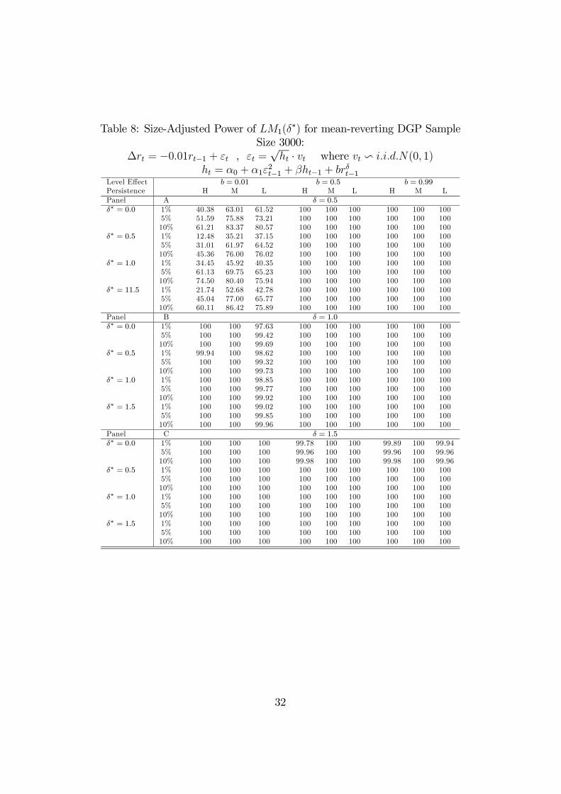
Table 8: Size-Adjusted Power of LM1(δ∗) for mean-reverting DGP Sample

Size 3000:∆rt = −0.01rt−1 + εt , εt =


ht = α0 + α1ε2t−1 + βht−1 + brδt−1

Level Effect b = 0.01 b = 0.5 b = 0.99Persistence H M L H M L H M LPanel A δ = 0.5δ∗ = 0.0 1% 40.38 63.01 61.52 100 100 100 100 100 100

5% 51.59 75.88 73.21 100 100 100 100 100 10010% 61.21 83.37 80.57 100 100 100 100 100 100

δ∗ = 0.5 1% 12.48 35.21 37.15 100 100 100 100 100 1005% 31.01 61.97 64.52 100 100 100 100 100 10010% 45.36 76.00 76.02 100 100 100 100 100 100

δ∗ = 1.0 1% 34.45 45.92 40.35 100 100 100 100 100 1005% 61.13 69.75 65.23 100 100 100 100 100 10010% 74.50 80.40 75.94 100 100 100 100 100 100

δ∗ = 11.5 1% 21.74 52.68 42.78 100 100 100 100 100 1005% 45.04 77.00 65.77 100 100 100 100 100 10010% 60.11 86.42 75.89 100 100 100 100 100 100

Panel B δ = 1.0δ∗ = 0.0 1% 100 100 97.63 100 100 100 100 100 100

5% 100 100 99.42 100 100 100 100 100 10010% 100 100 99.69 100 100 100 100 100 100

δ∗ = 0.5 1% 99.94 100 98.62 100 100 100 100 100 1005% 100 100 99.32 100 100 100 100 100 10010% 100 100 99.73 100 100 100 100 100 100

δ∗ = 1.0 1% 100 100 98.85 100 100 100 100 100 1005% 100 100 99.77 100 100 100 100 100 10010% 100 100 99.92 100 100 100 100 100 100

δ∗ = 1.5 1% 100 100 99.02 100 100 100 100 100 1005% 100 100 99.85 100 100 100 100 100 10010% 100 100 99.96 100 100 100 100 100 100

Panel C δ = 1.5δ∗ = 0.0 1% 100 100 100 99.78 100 100 99.89 100 99.94

5% 100 100 100 99.96 100 100 99.96 100 99.9610% 100 100 100 99.98 100 100 99.98 100 99.96

δ∗ = 0.5 1% 100 100 100 100 100 100 100 100 1005% 100 100 100 100 100 100 100 100 10010% 100 100 100 100 100 100 100 100 100

δ∗ = 1.0 1% 100 100 100 100 100 100 100 100 1005% 100 100 100 100 100 100 100 100 10010% 100 100 100 100 100 100 100 100 100

δ∗ = 1.5 1% 100 100 100 100 100 100 100 100 1005% 100 100 100 100 100 100 100 100 10010% 100 100 100 100 100 100 100 100 100

32

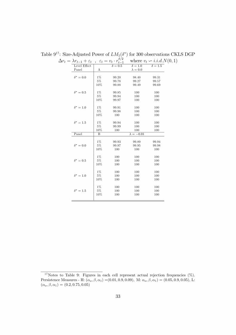
Table 917: Size-Adjusted Power of LM1(δ∗) for 300 observations CKLS DGP

∆rt = λrt−1 + εt , εt = vt · rδ/2t−1 where vt v i.i.d.N(0, 1)Level Effect δ = 0.5 δ = 1.0 δ = 1.5Panel A λ = 0.0

δ∗ = 0.0 1% 99.20 98.40 99.315% 99.78 99.27 99.5710% 99.88 99.49 99.69

δ∗ = 0.5 1% 99.85 100 1005% 99.94 100 10010% 99.97 100 100

δ∗ = 1.0 1% 99.91 100 1005% 99.98 100 10010% 100 100 100

δ∗ = 1.5 1% 99.94 100 1005% 99.99 100 10010% 100 100 100

Panel B λ = −0.01

1% 99.93 99.89 99.94δ∗ = 0.0 5% 99.97 99.95 99.98

10% 100 100 100

1% 100 100 100δ∗ = 0.5 5% 100 100 100

10% 100 100 100

1% 100 100 100δ∗ = 1.0 5% 100 100 100

10% 100 100 100

1% 100 100 100δ∗ = 1.5 5% 100 100 100

10% 100 100 100


33

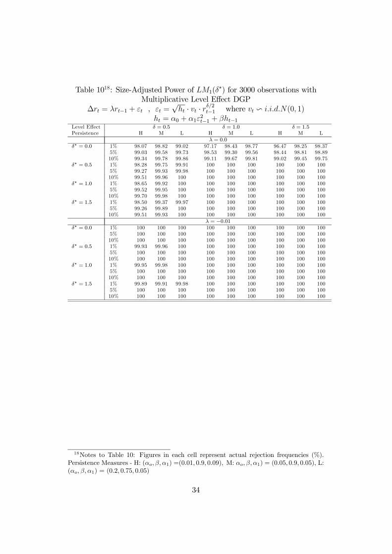
Table 1018: Size-Adjusted Power of LM1(δ∗) for 3000 observations with

Multiplicative Level Effect DGP∆rt = λrt−1 + εt , εt =

√ht · vt · rδ/2t−1 where vt v i.i.d.N(0, 1)

ht = α0 + α1ε2t−1 + βht−1

Level Effect δ = 0.5 δ = 1.0 δ = 1.5Persistence H M L H M L H M L

λ = 0.0δ∗ = 0.0 1% 98.07 98.82 99.02 97.17 98.43 98.77 96.47 98.25 98.37

5% 99.03 99.58 99.73 98.53 99.30 99.56 98.44 98.81 98.8910% 99.34 99.78 99.86 99.11 99.67 99.81 99.02 99.45 99.75

δ∗ = 0.5 1% 98.28 99.75 99.91 100 100 100 100 100 1005% 99.27 99.93 99.98 100 100 100 100 100 10010% 99.51 99.96 100 100 100 100 100 100 100

δ∗ = 1.0 1% 98.65 99.92 100 100 100 100 100 100 1005% 99.52 99.95 100 100 100 100 100 100 10010% 99.70 99.98 100 100 100 100 100 100 100

δ∗ = 1.5 1% 98.50 99.37 99.97 100 100 100 100 100 1005% 99.26 99.89 100 100 100 100 100 100 10010% 99.51 99.93 100 100 100 100 100 100 100

λ = −0.01δ∗ = 0.0 1% 100 100 100 100 100 100 100 100 100

5% 100 100 100 100 100 100 100 100 10010% 100 100 100 100 100 100 100 100 100

δ∗ = 0.5 1% 99.93 99.96 100 100 100 100 100 100 1005% 100 100 100 100 100 100 100 100 10010% 100 100 100 100 100 100 100 100 100

δ∗ = 1.0 1% 99.95 99.98 100 100 100 100 100 100 1005% 100 100 100 100 100 100 100 100 10010% 100 100 100 100 100 100 100 100 100

δ∗ = 1.5 1% 99.89 99.91 99.98 100 100 100 100 100 1005% 100 100 100 100 100 100 100 100 10010% 100 100 100 100 100 100 100 100 100


34

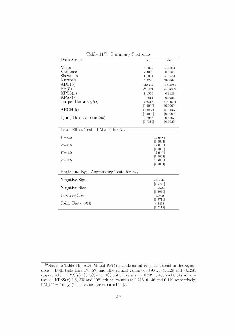
Table 1119: Summary StatisticsData Series rt ∆rt

Mean 6.1022 -0.0014Variance 7.3092 0.0665Skewness 1.1051 -0.5434Kurtosis 5.0226 20.9800ADF(5) -2.8718 -17.2931PP(5) -2.5476 -40.6889KPSS(µ) 1.1550 0.1129KPSS(τ) 0.7811 0.0224Jarque-Berra ∼ χ2(2) 758.13 27390.01

[0.0000] [0.0000]ARCH(5) 62.8979 61.0037

[0.0000] [0.0000]Ljung-Box statistic Q(5) 2.7986 0.5167

[0.7310] [0.9920]

Level Effect Test LM1(δ∗) for ∆rt

δ∗= 0.0 14.6480[0.0001]

δ∗= 0.5 17.0109[0.0002]

δ∗= 1.0 17.9194[0.0001]

δ∗= 1.5 18.6506[0.0001]

Engle and Ng’s Asymmetry Tests for ∆rt

Negative Sign -0.5644[0.5725]

Negative Size -1.2734[0.2030]

Positive Size -0.0356[0.9716]

Joint Test∼ χ2(3) 4.4458[0.2172]

19Notes to Table 11: ADF(5) and PP(5) include an intercept and trend in the regres-sions. Both tests have 1%, 5% and 10% critical values of -3.9642, -3.4128 and -3.1284respectively. KPSS(µ) 1%, 5% and 10% critical values are 0.739, 0.463 and 0.347 respec-tively. KPSS(τ) 1%, 5% and 10% critical values are 0.216, 0.146 and 0.119 respectively.LM1(δ

∗ = 0)∼ χ2(1). p-values are reported in [.].

35

Table 1220: Empirical Models of the U.S. Short Rate∆rt = µ+ λr + ϕCRASH + εt

E(ε2t |Ωt−1) = htCKLS Model: ht = brδt−1

Additive Model : ht = α0 + α1ε2t−1 + βht−1 + α2η

2t−1 + b

¡ rt−110

¢δMultiplicative Model : ht = φ2t r

δt−1;

φ2t = α0 + α1ε2t−1 + βφ2t−1 + α2η

2t−1

Additive Levels Models Multiplicative Levels ModelsCKLS AsyGARCHL AsyGARCH GARCHL GARCH AsyGARCHL GARCHL

µ 0.0215(0.0234)

−0.0057(0.0041)

−0.0019(0.0049)

−0.0057(0.0110)

−0.0028(0.0060)

−0.0028(0.0044)

−0.0019(0.0049)

λ −0.0037(0.0045)

0.0018(0.0011)

0.0006(0.0013)

0.0018(0.0009)

0.0007(0.0014)

0.0009(0.0011)

0.0008(0.0013)

ϕ 0.0559∗(0.0148)

0.1122∗(0.0507)

0.1129(0.0958)

0.1122∗(0.0364)

0.1134(0.0998)

0.1189∗(0.0489)

0.1143∗(0.0429)

α0 0.0002(0.0001)

0.0003∗(0.0001)

0.0002(0.0001

1.82× 10−11∗(2.10×10−22)

0.0011∗(0.0004)

0.0011∗(0.0005)

β1 0.7987∗(0.0499)

0.8471∗(0.0304)

0.7987∗(0.0494)

0.9105∗(0.0215)

0.8625∗(0.0336)

0.8686∗(0.0312)

α1 0.1628∗(0.0423)

0.1529∗(0.0304)

0.1628∗(0.0428)

0.0895∗(0.0215)

0.1375∗(0.0336)

0.1314∗(0.0312)

α2 1.23× 10−15∗(6.47×10−19)

0.0134(0.0211)

0.0458(0.0295)

b 6.52× 10−5∗(3.32×10−5)

0.0081∗(0.0034)

0.0081∗(0.0030)

δ 3.4325∗(0.2463)

3.4489∗(0.9978)

3.4489∗(1.0669)

0.1128∗(0.0412)

0.0989∗(0.0432)

Model DiagnosticsL · 2734.2977 2701.1121 2734.2977 2667.8615 2726.8174 2722.8223Q(5) 0.0000∗ 0.0000∗ 0.0000∗ 0.0000∗ 0.0000∗ 0.0000∗ 0.0000∗Q2(5) 0.0000∗ 0.6695 0.6973 0.6695 0.4264 0.7484 0.7509Hansen J- Test χ2

(1)=2.037533 [0.1535]

Davies Bound TestH0 : b = 0 AsyGARCHL and AsyGARCH: P(LR>66.3712) = 2.55× 10−14

GARCHL and GARCH: P(LR>132.8724) = 1.29× 10−28

20Notes to Table 12: Standard errors are reported in (.). * indicates that the coefficientis significant at 5% significance level. The p-values of the Ljung-Box test statistic arereported

36

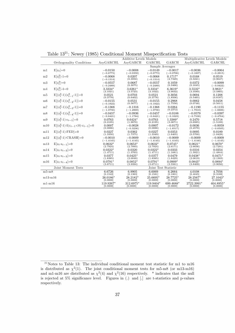
Table 1321: Newey (1985) Conditional Moment Misspecification TestsAdditive Levels Models Multiplicative Levels Models

Orthogonality Conditions AsyGARCHL AsyGARCH GARCHL GARCH AsyGARCHL GARCHLSample Averages

m1 E[zt]=0 −0.0150(−0.6773)

−0.0008(−0.0359)

−0.0149(−0.6773)

−0.0017(−0.0706)

−0.0036(−0.1607)

−0.0064(−0.2815)

m2 E[z2t ]-1=0 −0.0068(−0.1314)

0.0207(0.3950)

−0.0068(−0.1314)

0.1717∗(2.7329)

0.0168(0.3221)

0.0519(0.9647)

m3 E[z3t ]=0 −0.0557(−0.2489)

0.0687(0.3075)

−0.0557(−0.2489)

0.1059(0.3466)

0.0372(0.1645)

−0.0099(−0.0422)

m4 E[z3t ]-4=0 3.3334∗(3.1021)

3.6261∗(3.5723)

3.3334∗(3.1022)

6.3619∗(3.9032)

3.5532∗(3.3589)

3.9821∗(3.5865)

m5 E[(z2t -1)(z2t−1-1)]=0 0.0521

(0.3778)0.0703(0.6402)

0.0521(0.3778)

0.3056(1.8506)

0.0694(0.5465)

0.1208(0.8187)

m6 E[(z2t -1)(z2t−2-1)]=0 −0.0155

(−0.1922)0.0531(0.5677)

−0.0155(−0.1922)

0.2968(1.7558)

0.0062(0.0748)

0.0458(0.5011)

m7 E[(z2t -1)(z2t−3-1)]=0 −0.1368

(−1.0756)−0.1316(−1.2869)

−0.1368(−1.0756)

0.0264(0.2372)

−0.1190(−1.7910)

−0.1155(−1.6606)

m8 E[(z2t -1)(z2t−4-1)]=0 −0.0457

(−0.6421)−0.0936(−1.1784)

−0.0457(−0.6421)

−0.0188(−0.1623)

−0.0579(−0.7538)

−0.0397(−0.4764)

m9 E[(z2t -1)·rt−1]=0 0.0763(0.2195)

0.6424∗(1.9870)

0.0763(0.2195)

1.3389∗(3.0671)

0.2470(0.6985)

0.5718(1.5189)

m10 E[(z2t -1)·I(εt−1<0)·εt−1]=0 0.0007(0.0886)

−0.0028(−0.3236)

0.0007(0.0886)

−0.0172(−1.6517)

0.0036(0.4578)

−0.0059(−0.6505)

m11 E[(z2t -1)·FED]=0 0.0227(1.3350)

0.0362(1.7375)

0.0227(1.3349)

0.0353(1.6405)

0.0095(0.5700)

0.0189(1.0428)

m12 E[(z2t -1)·CRASH]=0 −0.0010(−1.4145)

−0.0009(−1.4145)

−0.0010(−1.4145)

−0.0009(−1.4145)

−0.0009(−1.4146)

−0.0009(−1.4145)

m13 E[zt·zt−1]=0 0.0632∗(2.7924)

0.0653∗(2.7893)

0.0632∗(2.7924)

0.0745∗(2.6171)

0.0621∗(2.6636)

0.0670∗(2.7291)

m14 E[zt·zt−2]=0 0.0322∗(1.4711)

0.0320(1.3763)

0.0322∗(1.4711)

0.0333(1.1681)

0.0316(1.3921)

0.0354(1.4844)

m15 E[zt·zt−3]=0 0.0377(1.8385)

0.0425∗(2.0040)

0.0377(1.8385)

0.0479(1.8429)

0.0438∗(2.0619)

0.0471∗(2.1303)

m16 E[zt·zt−4]=0 0.0791∗(3.6711)

0.0852∗(3.9394)

0.0791∗(3.6711)

0.0909∗(3.5561)

0.0843∗(3.8409)

0.0894∗(3.9056)

Joint Moment Tests Joint Test Statisticm5-m8 6.6726

[0.1542]6.9905[0.1363]

6.6069[0.1581]

6.2664[0.1801]

4.0108[0.4045]

4.7056[0.3188]

m13-m16 26.0186∗[0.0000]

28.2182∗[0.0000]

25.6695∗[0.0000]

28.7725∗[0.0000]

28.2567∗[0.0000]

27.1043[0.0000]

∗

m1-m16 119.9267∗[0.0000]

312.6975[0.0000]

∗ 119.9404∗[0.0000]

699.4688∗[0.0000]

2722.3991∗[0.0000]

404.8955∗[0.0000]

21Notes to Table 13: The individual conditional moment test statistic for m1 to m16is distributed as χ2(1). The joint conditional moment tests for m5-m8 (or m13-m16)and m1-m16 are distributed as χ2(4) and χ2(16) respectively. * indicates that the nullis rejected at 5% significance level. Figures in (.) and [.] are t-statistics and p-valuesrespectively.

37

Table 1422: Models of the U.S. Short Rate Corrected for Serial Correlation∆rt = µ+ λrt−1 + Σ4i=1ρi∆rt−i + ϕCRASH + εt

E(ε2t |Ωt−1) = htAdditive Model : ht = α0 + α1ε

2t−1 + βht−1 + α2η

2t−1 + b

¡ rt−110

¢δMultiplicative Model : ht = φ2t r

δt−1;

φ2t = α0 + α1ε2t−1 + βφ2t−1 + α2η

2t−1

Additive Levels Multiplicative Levelsµ −0.0034

(0.0038)0.0005(0.0045)

λ 0.0012(0.0010)

0.0002(0.0011)

ρ1 0.0520∗(0.0246)

0.0509(0.0274)

ρ2 0.0111(0.0236)

0.0133(0.0250)

ρ3 0.0216(0.0260)

0.0226(0.0244)

ρ4 0.1020∗(0.0238)

0.1045∗(0.0266)

ϕ 0.1038∗(0.0211)

0.1053∗(0.0263)

α0 0.0002(0.0002

0.0013∗(0.0005)

β1 0.7909∗(0.0507)

0.8636∗(0.0386)

α1 0.1663∗(0.0398)

0.1364∗(0.0386)

b 0.0089∗(0.0046)

δ 3.5818∗(1.0216)

0.1103∗(0.0530)

Standardised Residual DiagnosticsL 2734.7142 2724.6119Q(5) 0.3146 0.1866Q2(5) 0.6879 0.7255LR Test for Nested Models:Additive Models H0 : GARCHL vs. H1 : AsyGARCHL 1.32×10−5Multiplicative Models H0 : GARCHL vs. H1 : AsyGARCHL 3.34×10−3Davies Bound Test

GARCHL and GARCH: P(LR>131.1692) = 3.00× 10−28Joint Moment Testsm5-m8 6.6557

[0.1552]4.2706[0.3706]

m13-m16 9.1649[0.0571]

9.9458[0.0414]

m1-m16 98.3207∗[0.0000]

251.3580∗[0.0000]

22Note: See notes to Table 12 and 13. The LR test is distributed as a χ2(1).

38

Three Month Treasury Bill Yield1965 - 2003

1965 1968 1971 1974 1977 1980 1983 1986 1989 1992 1995 1998 20010.0

2.5

5.0

7.5

10.0

12.5

15.0

17.5

Changes in the Three Month Treasury Bill Yield1965 - 2003

1965 1968 1971 1974 1977 1980 1983 1986 1989 1992 1995 1998 2001-2.4

-1.6

-0.8

-0.0

0.8

1.6

2.4

Figure 1: rt and ∆rt

39

DEPARTMENT OF ECONOMICS - Faculty of Business and Economics

Documents