Department of Civil and Environmental Engineering Maseeh ...

A Route Improvement Algorithm for the Vehicle Routing Problem with Time Dependent Travel Times 

Miguel Andres Figliozzi

Department of Civil and Environmental Engineering

Maseeh College of Engineering and Computer Science

Portland State University

[email protected]

Abstract 

In urban areas, congestion creates a substantial variation in travel speeds during peak morning and evening hours. This research presents a new solution approach, an iterative route construction and improvement algorithm (IRCI), for the time dependent vehicle routing problem (TDVRP) with hard or soft time windows. Improvements are obtained at a route level; hence the proposed approach does not rely on any type of local improvement procedure. Further, the solution algorithms can tackle constant speed or time-dependent speed problems without any alteration in their structure. A new formulation for the TDVRP with soft and hard time windows is presented. Leveraging on the well known Solomon instances, new test problems that capture the typical speed variations of congested urban settings are proposed. Results in terms of solution quality as well as computational time are presented and discussed. The computational complexity of the IRCI is analyzed and experimental results indicate that average computational time increases proportionally to the square of the number of customers. KEYWORDS: Vehicle routing, time dependent travel time and speed, congestion.

1. Introduction Congestion is a common phenomenon in most urban areas of the world. Congestion creates a substantial variation in travel speeds during peak morning and evening hours. This is problematic for all vehicle routing models that rely on a constant value to represent vehicle speeds. Urban route designs that ignore these significant speed variations result in inefficient and suboptimal solutions. Poorly designed routes that lead freight vehicles into congested arteries and streets not only increase supply chain and logistics costs but also exacerbate externalities associated with freight traffic in urban areas such as greenhouse gases, noise, and air pollution. Travel time between customers and depot is found to be a crucial factor that exacerbates the negative impacts of congestion; congestion also affects carriers’ cost structure and the relative weight of wages and overtime expenses (Figliozzi, 2009). Routing models with time-varying travel times are gaining greater attention in vehicle routing literature and industry. However, research on the time dependent vehicle routing problem (TDVRP) is still comparatively meager in relation to the body of literature accumulated for the classical vehicle routing problem (VRP) and vehicle routing problem with time windows (VRPTW). In addition, published algorithms and related results can neither be readily benchmarked nor do they cover all practical and relevant objective functions or time window constraint types. The goals of this research are to: (a) formulate a time dependent vehicle routing problem with a general cost function and time window constraints, (b) present an intuitive and efficient solution methodology for time dependent problems, (c) introduce readily replicable time dependent instances and analyze the computational results, and (d) analyze the computational complexity of the solution approach. This paper is organized as follows: Section two presents a literature review for the TDVRP. Section three introduces notation and formulates the problems. Section four presents the iterative route construction and improvement algorithm (IRCI) to solve time dependent routing problems and minimize fleet size. Section five presents algorithms to reduce soft time window penalties and route durations. Section six presents benchmark problems. Section seven discusses computational results. Section eight analyses the worst case and average computational complexity of the algorithms presented in section four and five. Section nine concludes the paper.

2. Literature Review Unlike widely studied versions of the VRP, i.e. capacitated VRP or time windows VRP, time dependent problems have received considerably less attention. The time dependent VRP was first formulated by Malandraki and Daskin (1989, 1992) using a mixed integer linear programming formulation. A greedy nearest-neighbor heuristic based on travel time between customers was proposed, as well as a branch and cut algorithm to solve TDVRP without time windows. Hill and Benton (1992) considered a node based time dependent vehicle routing

problem (without time windows). Computational results for one vehicle and five customers were reported. Ahn and Shin (1991) discussed modifications to the savings, insertion, and local improvement algorithms to better deal with TDVRP. In randomly generated instances, they reported computation time reductions as a percentage of “unmodified” savings, insertion, and local improvement algorithms. Malandraki and Dial (1996) proposed a “restricted” dynamic programming algorithm for the time dependent traveling salesman problem, i.e. for a fleet of just one vehicle. A nearest-neighbor type heuristic was used to solve randomly generated problems. An important property for time dependent problems is the First In - First Out (FIFO) property (Ahn and Shin, 1991, Ichoua et al., 2003). A model with a FIFO property guarantees that if a vehicle leaves customer i to go to customer j at any time t, any identical vehicle with the same destination leaving customer i at a time t+ε, where ε >0, will always arrive later. This is an intuitive and desirable property though it is not present in all models. Earlier formulations and solutions methods, Malandraki and Daskin (1989, 1992), Hill and Benton (1992), and Malandraki and Dial (1996), do not guarantee the FIFO property as reported by Ichoua et al. (2003). Later research efforts have modeled travel time variability using “constant speed” time periods which guarantees the FIFO property, as shown by Ichoua et al. (2003). Ichoua et al. (2003) proposed a tabu search solution method, based on the work of Taillard et al. (1997), in order to solve time dependent vehicle routing problems with soft time windows. Ichoua et al. showed that ignoring time dependency, i.e. using VRP models with constant speed, can lead to poor solutions. Ichoua et al. tested their method using the Solomon problem set, soft time windows, three time periods, and three types of time dependent arcs. The objective was to minimize the sum of total travel time plus penalties associated with time window violations. Fleischmann et al. (2004) utilized route construction methods already proposed in the literature, savings and insertion, to solve uncapacitated time dependent VRP with and without time windows. Fleischmann et al. tested their algorithms in instances created from Berlin travel time data. Jung and Haghani proposed a genetic algorithm to solve time dependent problems (Jung and Haghani, 2001, Haghani and Jung, 2005). Using randomly generated test problems, the performance of the genetic algorithm was evaluated by comparing its results with exact solutions (up to 9 customers and 15 time periods) and a lower bound (up to 25 customers and 10 time periods). More recently Van Woensel et al. (2008) used a tabu search to solve the capacitated vehicle routing problem with time dependent travel times. To determine travel speed, approximations based on queuing theory and the volumes of vehicles in a link were used. Van Woensel et al. solved capacitated VRP (with no time windows) for between 32 and 80 customers. Donati et al. (2008) proposed a solution adapting the ant colony heuristic approach and a local search improvement approach that stores and updates the slack times or feasible delays. The heuristic was tested using a real life network in Padua, Italy, and some variations of the Solomon problem set.

Only two papers use well known benchmark problems with time windows. Ichoua et al. (2003) used the widely known Solomon problems for the VRP with time windows. However, capacity constraints were not considered, optimal fleet size was given, and no details were provided regarding how links were associated with “categories” that represent differences in the urban network (i.e. main arteries, local streets, etc.). Donati et al. (2008) also used Solomon instances, however, the results cannot be compared with previous results by Ichoua et al (2003) because a different time speed function was used and capacity constraints were considered. In addition, the exact instances used by Donati et al. (2008) cannot be reconstructed because the different travel speeds were randomly assigned to arcs. Therefore, no study can be swiftly replicated and solution qualities and computation times cannot be compared. Comparisons are also problematical because objective functions and routing constraints for time dependent problems are often dissimilar, unlike VRPTW research where the objective function is hierarchical and usually considers fleet size (primary objective), distance (secondary objective), and total route duration. Ichoua et al. (2003) study the TDVRP with soft time windows and consider as the objective function total duration plus lateness and assume that the optimal fleet size is given a priori. Haghani and Jung (2005) minimize the sum of costs associated with number of vehicles, distance, duration, and lateness. Fleischmann et al. (2004) minimize number of vehicles and total duration. Donati et al. (2008) optimizes fleet size (primary objective) and total route duration (secondary objective). Benchmark instances that can be clearly and unmistakably replicated by future researchers are detailed in Section six. The next section introduces mathematical notation and defines the problem under study.

3. Problem Definition Using a traditional flow-arc formulation (Desrochers et al., 1988), the time dependent vehicle routing problem with hard time windows studied in this research can be described as follows. Let ( , )G V A= be a graph where {( , ) : , }i jA v v i j i j V= ≠ ∧ ∈ is an arc set and the vertex set

is 0 1( ,...., )nV v v += . Vertices 0v and 1nv + denote the depot at which vehicles of capacity maxq

are based. Each vertex in V has an associated demand 0iq ≥ , a service time 0ig ≥ , and a

service time window [ , ]i ie l ; in particular the depot has 0 0g = and 0 0q = . The set of vertices

1{ ,...., }nC v v= specifies a set of n customers. The arrival time of a vehicle at customer

,i i C∈ is denoted ia and its departure time ib . Each arc ( , )i jv v has an associated constant

distance 0i jd ≥ and a travel time ( ) 0i j it b ≥ which is a function of the departure time from

customer i . The set of available vehicles is denoted K . The cost per unit of route duration is denoted tc ; the cost per unit distance traveled is denoted dc .

The primary objective function for the TDVRP is the minimization of the number of routes; the optimal number of routes is unknown. A secondary objective is the minimization of total time or distance. There are two decision variables in this formulation; k

ijx is a binary decision

variable that indicates whether vehicle k travels between customers i and j . The real decision

variable kiy indicates service start time for customer i served by vehicle k . The TDVRP is

formulated as follows:

0k

jk K j C

minimize x∈ ∈∑∑ , (1)

1 0 0( , )

( )k k k k kd ij ij t n j

k K i j A k K j C

minimize c d x c y y x+∈ ∈ ∈ ∈

+ −∑ ∑ ∑∑ , (2)

subject to:

maxk

i iji C j V

q x q∈ ∈

≤∑ ∑ , k K∀ ∈ (3)

1kij

k K j Vx

∈ ∈

=∑∑ , i C∀ ∈ (4)

0k kil lj

i V i V

x x∈ ∈

− =∑ ∑ , ,l C k K∀ ∈ ∀ ∈ (5)

0 1,0, 0k ki n ix x += = , ,i V k K∀ ∈ ∀ ∈ (6)

0 1kj

j V

x∈

=∑ , k K∀ ∈ (7)

, 1 1kj n

j V

x +∈

=∑ , k K∀ ∈ (8)

k ki ij i

j Ve x y

∈

≤∑ , ,i V k K∀ ∈ ∀ ∈ (9)

k ki ij i

j V

l x y∈

≥∑ , ,i V k K∀ ∈ ∀ ∈ (10)

, ,( ( ))k k k ki j i i i j i i jx y g t y g y+ + + ≤ , ( , ) ,i j A k K∀ ∈ ∀ ∈ (11)

{0,1}kijx ∈ , ( , ) ,i j A k K∀ ∈ ∀ ∈ (12) kiy ∈ℜ , ,i V k K∀ ∈ ∀ ∈ (13)

The primary and secondary objectives are defined by (1) and (2) respectively. The constraints are defined as follows: vehicle capacity cannot be exceeded (3); all customers must be served (4); if a vehicle arrives at a customer it must also depart from that customer (5); routes must start and end at the depot (6); each vehicle leaves from and returns to the depot exactly once, (7) and (8) respectively; service times must satisfy time window start (9) and ending (10) times; and service start time must allow for travel time between customers (11). Decision variables type and domain are indicated in (12) and (13). In the TDVRP with soft time windows, customer service time windows are defined by two intervals [ , ]i ie l and # #[ , ]i ie l where # #,i i i ie e l l≤ ≤ . The interval # #[ , ]i ie l indicates the interval of

time where service can start without incurring a penalty. The interval [ , ]i ie l indicates the

interval of time where service can start but there are additional costs, ec or lc , if service starts

early or late, respectively – i.e. during the early interval #[ , ]i ie e or during the late interval#[ , ]i il l . Defining e

ix and lix as auxiliary binary variables that indicate whether a penalty is

incurred, the objective functions can be expressed as follows:

li

i Cminimize x

∈∑ , i C∀ ∈ (14)

ei

i Cminimize x

∈∑ , i C∀ ∈ (15)

minimize

# #1 0 0

( , )

( ) ( ) ( )k k k k k k kd ij ij t n j e i i l i l

k K i j A k K j C k K i C k K i C

c d x c y y x c e y c y e+ ++

∈ ∈ ∈ ∈ ∈ ∈ ∈ ∈

+ − + − + −∑ ∑ ∑∑ ∑∑ ∑∑ (16)

subject to

#( )l k li i l ix y e x+− ≤ (17)

#( )e k ei i i ix e y x+− ≤ (18)

{0,1}eix ∈ , {0,1}l

ix ∈ (19) The primary objective function for the TDVRP with soft time windows is still the minimization of the number of routes. Using a customer service perspective ranking, a secondary objective is the minimization of the number of late penalties1 (14); a tertiary objective is the minimization of early penalties (15); a final objective is the minimization of the combined distance, route duration, and soft time window costs (16). Logical constraints (17) and (18) are used to determine if service times must be penalized due to early or late time window utilization, respectively. It is important to notice that the depot time windows as well as the maximum route duration are not changed as a result of the customers’ time window relaxation. The TDVRP with hard time windows is a special case of the soft time window formulation. If #

i ie e= and #i il l= ,

then (14) and (15) are redundant and (16) is reduced to (2). The travel time speed in any arc is a positive and continuous function of time, ( ) 0i js t > , which guarantees the FIFO property

(Ahn and Shin, 1991). In addition, in the presented TDVRP travel times may be asymmetrical, i.e. , ,( ) ( )k k

i j i j i jt y t y≠ even if k ki jy y= .

1 Although the cost of early and late service times are application dependent, in numerous real life problems early services are preferred over late services, e.g. blood transport, just-in-time production systems, express mail delivery, etc.

Unlike previous formulations of the TDVRP (Malandraki, 1989, Jung and Haghani, 2001) time is not partitioned into discrete intervals. Furthermore, the decision variable k

iy allows for waiting at customer i ; service start time may not necessarily be the same as arrival time. For example, if the vehicle arrives too early, it can wait at the customer location to avoid early service penalties. However, waiting may have an impact on future travel times. The following two sections describe a solution approach to tackle the TDVRP.

4. Solution Approach Time dependent travel times require significant modifications to local search approaches and metaheuristics that have been successfully applied to the traditional constant time VRPTW (Braysy and Gendreau, 2005a, Braysy and Gendreau, 2005b). A customer insertion or a local improvement not only influences the arrival and departure times of a “local” subset of customers but it may also significantly change travel times among “local” customers. Furthermore, the impact of altering a routing sequence is not just “local” but potentially affects all subsequent travel times. Changes in travel times have a subsequent impact on feasibility. To a certain degree, introducing soft time windows ameliorates the computational burden and loss of efficiency introduced by time dependent travel times. However, hard time constraints are more difficult to accommodate and this is reflected in the literature review. There are no published results in a set of standard benchmark problems with hard time windows and time dependent travel times. The presented IRCI solution approach for the TDVRP employs algorithms that do not require modifications to accommodate constant or time dependent travel speeds. The construction and improvement procedure are sequential and originally designed at the route level, i.e. it is not a local improvement. Hence, the presented algorithm produces routes for time dependent vehicle routing problems with hard and soft time windows with similar computation times. This research builds upon previous work to solve the VRP with soft and hard time windows (Figliozzi, 2008). The solution method to minimize fleet size is divided into two phases and algorithms: route construction and route improvement. A third algorithm, an auxiliary route building heuristic, is repeatedly executed during the execution of the construction heuristic. Similarly, the route construction algorithm is repeatedly executed during the execution of the improvement algorithms. Using a bottom up approach the algorithms are introduced in the following order: (a) an algorithm to sequence any given set of customers, (b) a route construction algorithm, and (c) a route improvement algorithm. In addition, due to the nature of the TDVRP, advancing or delaying service time may have a favorable impact on future travel times and costs. Hence another algorithm (d) is described in Section five to optimize service times given a set of routes obtained from (c). Travel time calculations are necessary to execute (a) to (d). However, unlike algorithms (a) to (d), travel time calculations are heavily dependent on the

specific type of speed function. Hence, the algorithm used to calculate travel times is presented in Appendix A for a specific type of speed function.

(a) The Auxiliary Routing Algorithm rH The auxiliary routing algorithm rH can be any heuristic that given a starting vertex, a set of customers, and a depot location returns a set of routes that satisfy the constraints of the TDVRP with soft or hard time windows. The auxiliary route heuristic is defined as

r 0( , , , )iv C vΔH where 0 1 6{ , ,...., }δ δ δΔ = are the parameters of the generalized cost function,

iv is the vertex where the first route starts, C is the set of customers to route, and 0v is the depot where all routes end and all additional routes start, with the exception of the first route which starts at iv . In this research, rH is a generalized nearest-neighbor heuristic (GNNH). The GNNH starts

every route k by finding, from a subset of C , the unrouted customer with the least appending “generalized cost”. At every subsequent iteration, the heuristic searches for the remaining unrouted customer with the least appending cost. Let i denote the initial vertex and let j

denote a potential customer to append next. Let kiq denote the remaining capacity of the

vehicle k after serving customer i . The service at customer i in route k begins at the earliest

feasible time, which is max( , )ki i iy a e= , and the departure time is given by k

i iy g+ . The generalized cost of going from customer i to customer j is estimated as:

1 2 3

# #4 5 6

g( , , , ) ( ) ( ( )) ( ( ( )))

( ) [ ] [ ]

k k k k kij i i j i i j i i ij i i

k k ki j j j j j

i j k d y g y y g l y g t y g

q q e y y e

δ δ δ

δ δ δ+ +

Δ = + + − + + − + + + +

+ − + − + − (20)

If customer j is infeasible, i.e. it cannot be visited after serving customer i , the cost of ending customer 'i s route and starting a new one to serve customer j is estimated as:

0 1 0 2 0 3 0 0

# #4 max 5 6

g( , , ) ( ) ( ( ))

( ) [ ] [ ]

kj j j j

k kj j j j j

i j d y e l t e

q d e y y e

δ δ δ δ

δ δ δ+ +

Δ = + + − + − +

+ − + − + − (21)

where 0δ is the cost of adding a new vehicle. The parameter 1δ takes into account the relative distance between customers and 2δ accounts for the “slack” between the completion of service at i and beginning of service at j . Following Solomon’s approach (Solomon, 1987), the parameter 3δ takes into account the “urgency” of serving customer j , expressed as the time remaining until the vehicle’s last possible service time start. The parameter 4δ takes into account the capacity slack of the

vehicle after serving customer j . The parameters 5δ and 6δ are added to account for possible early or late service penalties, respectively. (b) The Route Construction Algorithm cH In this algorithm, denoted cH , routes are constructed sequentially. Given a partial solution

and a set of unrouted customers, the algorithm uses the auxiliary heuristic rH to search for the

feasible least cost set of routes. The algorithm also uses an auxiliary function w( , ,g, )iv C W

that, given a set of unrouted customers C , a vertex ,i iv v C∉ , and a generalized cost function

g( , , , )i j kΔ , returns a set of vertices of cardinality | |W with the lowest generalized costs g( , , , )i j kΔ for all jv C∈ .

Parameters:

rH : Route building heuristic.

W : Width of the search, the number of solutions to be built and compared before adding a customer to a route, | |w C≤ . Δ : Search space of the route heuristic generalized cost parameters

Data: C : Set of customers to route

0 :v the depot

:iv initial vertex START cH

0start v← 1

lowestCost ←∞ 2

0bestSequence v← 3

for each Δ∈Δ 4 while C ≠∅ do 5

* w( , ,g, )C start C W← 6 for each *

iv C∈ 7

if r 0c( ( , , , ))ibestSequence v C v∪ ΔH < lowestCost then 8

r 0c( ( , , , ))ilowestCost bestSequence v C v← ∪ ΔH 9

ilowestNext v← 10 end if 11

end for 12 start lowestNext← 13

\C C lowestNext← 14 bestSequence bestSequence lowestNext← ∪ 15

r 0( , , , )R bestSequence lowestNext C v← ∪ ΔH 16 end while 17

end for18 Output: Best set of routes R that serve all C customers END cH This algorithm will sequentially construct routes. In line 7, up to W “potentially” good candidates are selected. In lines 9 to 11 complete routes, built using the W candidates and the heuristic rH , are compared. The candidate with the least generalized cost is selected. The

generalized cost function g that is used in rH must not be confused with the objective cost

function c that is used in cH or the improvement heuristic iH ; the latter cost function is the sum of the accrued vehicle, distance, time, or penalty costs as indicated in the objective function. (c) The Route Improvement Algorithm iH The route construction algorithm generates an initial grouping or clustering of customers. Any route obtained from cH is a special cluster of customers; a cluster of customers with the desirable property that there is at least one feasible sequence that satisfies all the constraints of the TDVRP. Fleet size and routing costs can be further reduced using a route improvement algorithm. The improvement algorithm works on a subset of routes. The motivation of the route improvement algorithm is to combine these routes, “feasible clusters”, to consolidate or improve the efficiency of routes that are not fully utilized in terms of vehicle capacity, route duration, number of customers serviced, etc. In the iH algorithm

two functions are introduced. The function k ( , )s R s orders the set of routes R from smallest to largest based on the number of customers per route and then returns a set of 1s ≥ routes with the least number of customers; e.g. k ( ,1)s R will return the route with the least number of customers. The number of customers per route is used as a proxy measure of potential route capacity utilization. If two or more routes have the same number of customers, ties are solved drawing random numbers. The function k ( , , )g ir S p returns a set of p routes that belong to S and are good “matches”

for route ir . Good “matches” refers to routes that as a group have the potential to be consolidated or improved. In this research two measures are used to evaluate the quality of a potential “match”: (1) Geographical proximity, the distance between any two routes’ center of

gravity is used as a proxy measure of geographic proximity assuming that close routes have the potential to be improved and (2) Utilization, the number of customers per route is used as a proxy measure of potential route capacity utilization assuming that routes are poorly utilized have the potential to be combined. By definition, the route ir is always included in the output

of the set function k ( , , )g ir S p . To simplify notation the term ( )C G is the set of customers

served by the set of routes G . Data: R : Set of routes

Parameters:

cH : Route building heuristic

W : Number of solutions to be built and compared in the construction heuristic Δ : Generalized cost parameters of the auxiliary route heuristic s : Number of routes potentially considered for improvement p : Number of neighboring routes that are reconstructed k s and k g : route selection functions

START iH

min( ,| |)s s R← 1 min( , )p s p← 2 k ( , )sS R s R← ⊆ 3

' \S R S← 4 * k ( ,1)sr S← 5

while | | 1S > do 6 *k ( , , )gG r S p← 7

c' ( , , , ( ))rG W C G← ΔH H 8

if c( ')G < c( )G then 9 \R R G← 10 'R R G← ∪ 11

\S S G← 12 'S S G← ∪ 13

* k ( ,1)sr S← 14

end if 15 \ k ( ,| | 1)sr S S S← − 16

\S S r= 17 if | ' | 0S > then 18

' k ( ',1)sr S= 19

' '/ 'S S r← 20 'S S r← ∪ 21

end while22 Output: R set of improved routes

END iH The smallest route is selected in line 6 using function k s while “matching” routes are selected

in line 7 using function k g . The routes are reconstructed in line 8. If the generalized cost is

improved (line 9), the routes with the least generalized cost are selected. The algorithm continues adding new routes until all routes have had at least one opportunity to be reconstructed and “re-optimized”.

5. Service Time Improvement The previous algorithms deal with the minimization of costs via sequencing of customers and their assignment to routes. The yH algorithm aims at reducing costs by improving customer

service start times for a given set of routes produced by iH . For any given route, a dynamic programming approach can be used to determine the optimal service start times k

iy for customer i belonging to route k given the arrival time ia : each

customer is associated with a stage, the decision variable is the service time kiy , and the state

is defined by the arrival time ia . For any given route k defined by the sequence of customers(0,1,2,..., , 1)q q + where 0 and 1q + denote the depot. If the cost to minimize is the sum of

distance traveled, route durations, and soft time window utilization given by expression(16), the cost function, ( , )q qy aπ , for the last customer is 2:

# #, 1 1( , ) ( ) ( ) ( )k k

q q d q q t q q e q q l q ly a c d c a y c e y c y eπ + ++ += + − + − + − (22)

where 1 , 1( )q q q q q q qa y g t y g+ += + + + and subject to q q ql y a≥ ≥ .

Using a backward solution approach, for each customer it is possible to define a stage cost and an optimal cost to go function. Further, for each customer, it is possible to limit the feasible space of customer service time to a closed time interval. For a customer i belonging

to route k , let kiy and k

iy denote, respectively, the earliest and latest feasible service times.

2 The distance term can be eliminated from (22) because it is not affected by service time.

Lemma 1: given any route k , the optimal service times at any customer i belong to the time interval [ , ]k k

i iy y and can be calculated using a forward and backward algorithm. Proof: starting from the depot, earliest possible arrival at customer 1 is 1 0 01 0( )a e t e= + due to

FIFO property; earliest service time at customer 1 is 1 1 1max( , )ky a e= ; earliest departure at

customer 1 is 1 1ky g+ . Earliest possible arrival at customer 2 is 2 1 1 1,2 1 1( )k ka y g t y g= + + +

due to FIFO property; earliest service time at customer 2 is 2 2 2max( , )ky a e= ; earliest

departure at customer 2 is 2 2ky g+ and so on until reaching the last customer.

Starting from the depot, latest possible departure time from customer q is:

, 1 1arg max , . .( ( ) )y q q qy s t y t y l∈ℜ + ++ ≤ ; due to the continuous speed function and the FIFO

property this value is unique. The latest possible service time at customer q is

min( , )kq q qy y g l= − . Latest possible departure time from customer 1q− is

1,arg max , . .( ( ) )ky q q qy s t y t y y∈ℜ −+ ≤ ; latest possible service time at customer 1q− is

1 1 1min( , )kq q qy y g l− − −= − and so on until reaching the first customer.

Based on the workings of the algorithms , ,r cH H and iH it is possible to state properties that simplify the determination of service start times. Property 1: Given a route k outputted by iH , the customer service times are the earliest feasible times. Proof: Due to the workings of the rH algorithm, the service at any customer i in route k begins at the earliest feasible time, which is max( , )k k

i i i iy y a e= = , and the departure time is

given by ki iy g+ . Due to the FIFO property, for the given routes, customers cannot be

serviced earlier than the provided service start times. Property 2: Given a route k outputted by iH , total route duration cannot be reduced. Proof: Due to Property 1, service times cannot be advanced. Then, the FIFO property guarantees that route duration cannot be reduced further unless the set of routes is altered. The arrival times at each customer are the earliest possible for the sequence given by route k . Property 3: Given a route k outputted by iH , a TDVRP with hard time windows requires no service time optimization for route k . Proof: Due to Property 2, route durations cannot be reduced. Start times do not affect distance traveled and there are no soft time windows penalties or costs to be reduced. Hence, altering service start time will not reduce any objective function. Property 4: Given a route k outputted by iH , if a customer uses the “late” soft time window, no improvement can be made by changing the service time.

Proof: Due to property 1, the service time cannot be advanced without losing feasibility. If the service time is delayed, there is a greater late penalty. Hence, if a customer in the route outputted by iH uses a late time window, the provided service time for that customer cannot be improved. Corollary: In a route outputted by iH , the service time optimization problem can be decomposed into smaller problems delimited by customers using “late” soft time windows. Service Time Improvement Algorithms (d) For each customer that uses an early soft time window, the ybH algorithm attempts to reduce

early soft time window usage without allowing the introduction of service delays that increase late time window usage. This algorithm operates backwards. For the sake of presentation simplicity, periods of constant travel time are assumed. The depot working time 0 0[ , ]e l is

partitioned into p time periods 1 2, , ..., pT T T=T ; each period kT has an associated constant

travel speed ks in the time interval [ , ]k k kT t t= .

Data:

T and S : time intervals and speeds

, ,i j jv v y : two customers served in this order in route k , kjy is the current service

time at customer j START ybH

if # &k k kj j j jy l y y< < then 1

#min( , )k kj j jy l y← 2

end if 3 find k, k

k j kt y t≤ ≤ 4

/ki j ji kb y d s← − 5

, kji jd d t y← ← 6

while i kb t< do 7

( )k kd d t t s← − − 8

kt t← 9

1/i kb t d s +← − 10 1k k← + 11

end while 12 min( , )k

i i i iy b g l← − 13 Output:

,k kj iy y

END ybH

After early time windows have been reduced, a final task is to reduce route duration without increasing the number of soft or late time windows. The following forward algorithm, yfH ,

reduces route duration without increasing soft time windows. Data:

T and S : time intervals and speeds

, ,i j jv v y : two customers served in this order in route k , kiy is the current service

time at customer j START yfH

if # &k k ki j i iy e y y> > then 1

#max( , )k ki i iy e y← 2

end if 3 find k, k

k i kt y t≤ ≤ 4

/kj i ij ka y d s← + 5

, kij id d t y← ← 6

while j ka t> do 7

( ) kkd d t t s← − − 8

kt t← 9

1/j ka t d s +← + 10

1k k← + 11 end while 12

max( , )kj j jy a e← 13

Output: ,k k

i jy y

END yfH Both algorithms try to reduce the interval [ , ]k k

i iy y where the optimal service start time is found for a

given a route k .

6. Proposed Benchmark Problems As mentioned in section two, results provided in previous research efforts cannot be compared in terms of solution quality or computational time. This is revealing of a still incipient body of work for the TDVRP. The proposed set of benchmark problems are based on the classical instances of the VRP with time windows proposed by Solomon (1987). The

Solomon instances include distinct spatial customer distributions, vehicles’ capacities, customer demands, and customer time windows. These problems have not only been widely studied in the operations research literature but the datasets are readily available3. The well-known 56 Solomon benchmark problems for vehicle routing problems with hard time windows are based on six groups of problem instances with 100 customers. The six problem classes are named C1, C2, R1, R2, RC1, and RC2. Customer locations were randomly generated (problem sets R1 and R2), clustered (problem sets C1 and C2), or mixed with randomly generated and clustered customer locations (problem sets RC1 and RC2). Problem sets R1, C1, and RC1 have a shorter scheduling horizon, tighter time windows, and fewer customers per route than problem sets R2, C2, and RC2 respectively. This section proposes new test problems that capture the typical speed variations of congested urban settings. The problems are divided into three categories of study: (1) constant speed Solomon instances, (2) time dependent problems with hard time windows, and (3) time dependent problems with soft time windows. Some previous research efforts may have used standard problems but they allocated travel speed distributions randomly to customer arcs or it is ambiguous the type of time dependency allocated to each arc. In order to provide readily replicable instances, the travel speed distributions apply to ALL arcs among customers, i.e. in the arc set:

{( , ) : , }i jA v v i j i j V= ≠ ∧ ∈ .

Most recent research efforts, as stated in section two, have used constant speed intervals. The same approach is adopted in this research because constant speed intervals guarantee the FIFO property and can be readily replicated. The algorithm used to calculate travel times is presented in Appendix A. 1. Constant speed problems with hard time windows Constant travel speed is a special case of the general time dependent problem. These instances are the classical Solomon problems that have been widely studied and provide an indication of the performance of the algorithm with constant travel speed. 2. Time dependent problems with hard time windows These instances introduce fast periods between depot opening and closing times. The depot working time 0 0[ , ]e l is divided into five time periods of equal durations:

[0, 0.2 0l ); [0.2 0l , 0.4 0l ); [0.4 0l , 0.6 0l ); [0.6 0l , 0.8 0l ); and [0.8 0l , 0l ]. and the corresponding travel speeds are: TD1 = [1.00 , 1.60, 1.05 , 1.60, 1.00], TD2= [1.00 , 2.00, 1.50 , 2.00, 1.00], TD3 = [1.00 , 2.50, 1.75 , 2.50, 1.00].

3 Several websites maintain downloadable datasets of the instances including Solomon’s own website: http://web.cba.neu.edu/~msolomon/problems.htm

If the vehicles were to travel non-stop in the interval 0 0[ , ]e l the vehicle would travel an extra 25%, 50%, and 75% more for speeds TD1, TD2, and TD3 respectively than in the original Solomon instances. 3. Time dependent problems with soft time windows These instances introduce two congested periods between depot opening and closing times. The depot working time 0 0[ , ]e l is divided into the same five periods and the corresponding travel speeds are: TD4 = [1.10 , 0.85, 1.10 , 0.85, 1.10], TD5 = [1.20 , 0.80, 1.00 , 0.80, 1.20], TD6 = [1.20 , 0.70, 1.20, 0.70, 1.20]. If one vehicle were to travel non-stop in the interval 0 0[ , ]e l , this vehicle would travel the same distance as in the original Solomon instances but with increasing travel speed variability, i.e. same average speed but with increased variability. However, soft time windows are required because some Solomon problems would be infeasible otherwise (Ichoua et al., 2003, Donati et al., 2008). An allowable time window violation per customer equal to:

# #max 0 00.1( ) i i i iP l e e e l l= − = − = −

is allowed. However, the depot working time 0 0[ , ]e l is not relaxed. The penalty cost for an early or late delivery is one unit of cost per unit time which is the same value used in constant speed Solomon instances with soft time windows (Balakrishnan, 1993, Chiang and Russell, 2004).

7. Experimental Results Proper benchmarking of algorithms, solution quality and computation times can be performed using standardized instances and computers. However, computation times can be difficult to compare if there are significant differences in computer processing power or equipment. Detailed information regarding computer equipment (brand, model, processor, RAM) can be used to estimate relative computer power using Dongarra (2007) and SPEC4 results. All the results presented in this section were obtained with a laptop Dell Latitude D430, with an Intel Core CPU 1.2 GHz and 1.99 GB of RAM. Even after standardizing problems and equipment there may be differences in running time due to different compilers, programming language, or code efficiency and implementation. As indicated by Cordeau et al. (2002), results presented in the VRP literature usually present better results on benchmark problems at the expense of (a) too many parameters or complicated coding that lacks flexibility to accommodate real-life constraints, (b) too many

4 Comparison among computers can be found at http://www.specbench.org/

parameters that are difficult to calibrate or even understand, and (c) solution approaches that are markedly tailored to perform well on the benchmark problems but that may lack generality and robustness in real-life problems. Golden et al. (1998) indicates that algorithms should be compared not only by the number of parameters but also by how intuitive and reasonable these parameters are from a user’s perspective. To avoid excessive “tailoring”, all the results presented in this research use the exact same procedure and parameter values in all cases, i.e. the same code, with the parameters described in Section four, and the same parameter values. The exact same parameters are used not only in different types of problems, e.g. soft vs. hard, but also in different types of instances, e.g. R1 and C2. Travel time calculations were performed using the algorithm presented in Appendix A. It is also assumed that the algorithm does not “know” anything regarding the type of problem or its characteristics, e.g. average number of customers per route, binding constraints, or lower bounds. This type of information can be exploited to reduce computational times, e.g. usage of lower bounds (Figliozzi, 2008), but if new parameters, steps, or lines of code are needed they have to be explicitly stated to provide a level playing field when it comes to comparisons among algorithms.

1) Constant speed problems with soft time windows The first set of results corresponds to the extensively studied Solomon instances with constant travel speeds; results are presented in Table 1. In these instances the primary objective is to minimize the number of vehicles and the secondary objective to minimize travel distance. The first row presents the combination of the absolute best solutions found to date which have been obtained by different researchers, algorithms, machines, and computational times (Donati et al., 2008, SINTEF, 2008).

Table 1. VRPTW Results for classical Solomon Instances – Constant Speed Average Number of Vehicles by Problem Class    

Method  R1  R2  C1  C2  RC1  RC2 

(1) Best  Ever (1987‐…)  11.92 2.73 10.00 3.00 11.50  3.25(2) Taillard et al. (1997)  12.64 3.00 10.00 3.00 12.08  3.38(3) Donati et al.  (2008)  12.61  3.09  10.00  3.00  12.04  3.38 (4) IRCI  12.58  3.00  10.00  3.00  12.12  3.38 

Average Distance                   

Method  R1  R2 C1 C2 RC1  RC2

(1) Best  Ever (1987‐…)  1,210  952  828  590  1,384  1,119 (2) Taillard et al. (1997)  1,220 1,013 828 591 1,381  1,199(2) Donati et al.  (2008)  1,199  967  828  590  1,374  1,156 (4) IRCI  1,248  1,124  841  626  1,466  1,308 

Computation time for all 56 problems: (1) different authors, machines and computation times; (2) Sun Sparc 10, 261 min; (3) Pentium IV 2.66 GHz, 168 min (4) Dell Latitude D430, 1.2 GHz, 19.0 min 

The second row presents the results of Taillard et al. (Taillard et al., 1997) using the tabu search algorithm for soft time window problems and constant travel speed that was

implemented by Ichoua et al (Ichoua et al., 2003). Taillard et al. reported better results but at the expense of significantly longer computational times. The results reported by Taillard et al. and Donati et al. are average results and computation times over independent runs. The performance of the IRCI algorithm, in relation to other approaches that can solve problems with both soft and hard time windows have been used in time dependent problems, is somewhat comparable. The IRCI solutions have relatively low computational times – an average of 21.3 seconds for each 100 customer problem but comparisons in terms of speed with Taillard et al. (1997) are difficult. Computers and their architecture have evolved significantly in the last 10 years. However, the IRCI is faster than the method presented by Donati et al (2008). In terms of solution quality, the IRCI is outperformed by the best local search approaches (Braysy and Gendreau, 2005b). The IRCI solutions are, on average, slightly less than 4% from the best results ever obtained for the Solomon instances with constant travel times. The IRCI can obtain slightly better performances, around 3%, in terms of number of vehicles with longer computational times or by tailoring some parameters to each problem type. However, to avoid any kind of “distortion”, the same general code is utilized to obtain all the results presented in this section.

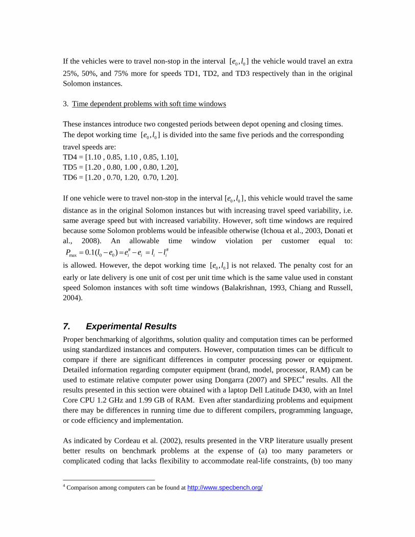
Table 2. VRPTW Results – Hard Time Windows Average Number of Vehicles by Problem Class   

Travel time Distribution  R1  R2  C1  C2  RC1  RC2 

(1) TD1  11.67  2.82  10.00  3.00  11.38  3.25 (2) TD2  10.75  2.55  10.00  3.00  10.50  2.88 (3) TD3  9.92  2.27  10.00  3.00  10.00  2.75 

Average Distance                   

Travel time Distribution  R1  R2  C1  C2  RC1  RC2 

(1) TD1  1,295 1,216 879 657 1,405  1,444(2) TD2  1,258  1,244  864  654  1,395  1,454 (3) TD3  1,237  1,269  880  697  1,362  1,434 

Average Travel Time             

Travel time Distribution  R1 R2 C1 C2 RC1  RC2

(1) TD1  1,080  990  729  563  1,164  1,177 (2) TD2  897  861  644  495  989  993 (3) TD3  793 774 608 485 860  867

Computation time for all 56 problems: (1) TD1,  19.1 min; (2) TD2, 17.7 min;  (3) TD3, 17.3 min – in all cases using Dell Latitude D430, 1.2 GHz 

2) Time dependent problems with hard time windows

The second set of results corresponds to the Solomon instances with time dependent travel speeds and soft time windows. In these instances the primary objective is to minimize the number of vehicles, the secondary objective is to minimize time and distance traveled. To the best of the author’s knowledge this is the first reporting of Solomon instances with hard time windows and time dependent speeds; results are presented in Table 2. As expected,

with increased travel speeds, the number of vehicles is reduced significantly. However, there is relatively minimal change in the distance traveled. Time traveled decreases as average travel speed increases though not at the same rate. Results for problem sets C1 and C2 are largely unchanged due to the binding constraint of the vehicle capacity.

3) Time dependent problems with soft time windows The second set of results corresponds to the Solomon instances with time dependent travel speeds and soft time windows; results are presented in Table 3. In these instances the primary objective is to minimize number of vehicles, the secondary objective is to minimize time window violations, and the tertiary objective is to minimize the soft time window penalties and distance traveled. Table 3 presents the results in terms of fleet size, distance, and travel time.

Table 3. VRPTW Results – Soft time windows Average Number of Vehicles by Problem Class    

Travel time Distribution  R1  R2 C1 C2 RC1  RC2

(1) TD4  10.42  2.82  10.00  3.00  10.50  3.00 (2) TD5  10.42 2.64 10.00 3.00 10.63  3.00(3) TD6  10.58  2.73  10.00  3.00  10.75  3.00 

Average Distance       

Travel time Distribution  R1  R2  C1  C2  RC1  RC2 

(1) TD4  1,142  1,010  856  666  1,241  1,135 (2) TD5  1,131  1,016  860  665  1,226  1,156 (3) TD6  1,127  1,016  869  660  1,236  1,149 

Average Travel Time             

Travel time Distribution  R1  R2  C1  C2  RC1  RC2 

(1) TD4  1,139 1,023 871 669 1,237  1,150(2) TD5  1,134  1,039  884  672  1,220  1,184 (3) TD6  1,143  1,061  938  685  1,253  1,213 

Computation time for all 56 problems: (1) TD4,  19.5 min; (2) TD5, 19.6 min;  (3) TD6, 19.4 min – in all cases using Dell Latitude D430, 1.2 GHz 

The travel speed distributions TD4, TD5, and TD6 are listed in increasing order of travel speed variability. Without changing overall average speed, travel speed variability worsens the results in terms of number of vehicles for R1 and RC1 problems. Results in terms of distance traveled have little variation. Travel time slightly increases. Problem sets C1 and C2 are mostly unchanged because the binding constraint is vehicle capacity. As customary in the VRP with time windows literature, Table 4 reports the number of soft time windows used, broken down into early and late service times as well as the penalty paid for early or late services. Usage of early soft time windows is more prevalent than the usage

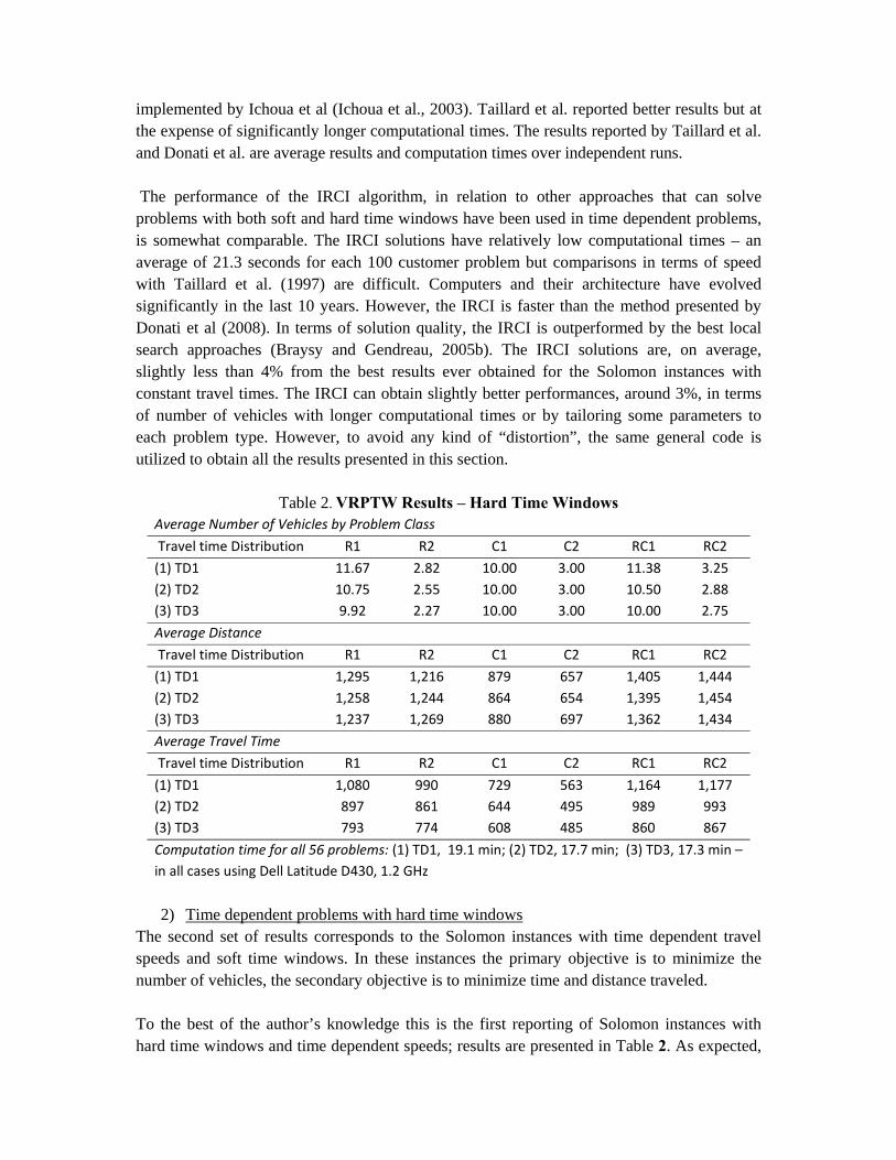
of late time windows. As expected, time window violations and penalties decrease as the number of vehicles used increases.

Table 4. VRPTW Results – Soft time windows Average Number of Soft Time Windows (early)    

Travel time Distribution  R1  R2 C1 C2 RC1  RC2

(1) TD4  20.5  20.1  15.8  18.6  21.1  21.3 (2) TD5  20.4 19.9 18.6 14.9 22.1  21.1(3) TD6  20.4 20.1 16.1 13.9 21.3  21.5

Average Number of Soft Time Windows (late) 

Travel time Distribution  R1  R2  C1  C2  RC1  RC2 

(1) TD4  18.0  13.6  8.2  17.0  16.3  14.1 (2) TD5  17.5  12.5  8.7  10.4  14.5  14.8 (3) TD6  15.8  12.5  6.2  8.4  15.1  15.1 

Soft Time Window Penalties (early)    

Travel time Distribution  R1  R2 C1 C2 RC1  RC2

(1) TD4  386.6 1,516.3 516.5 3,025.5 381.7  1,718.9(2) TD5  425.1 1,609.4 861.5 1,467.7 448.5  1,664.4(3) TD6  419.3  1,559.1  657.2  1,697.8  446.2  1,508.2 

Soft Time Window Penalties   (late)

Travel time Distribution  R1  R2  C1  C2  RC1  RC2 

(1) TD4  210.4  681.2  480.5  3,267.1  197.8  695.9 (2) TD5  208.2  637.6  547.6  1,797.7  173.2  692.1 (3) TD6  187.6 629.5 363.2 1,708.8 189.2  787.8

8. Computational Complexity The relative simplicity of the IRCI allows for a straightforward algorithmic analysis. The auxiliary heuristic rH is called by the construction algorithm no more than | |nW Δ times; where n is the number of customers. Hence, the asymptotic number of operations of the construction algorithm is of order r( | | ( ( ) ) )nW O nΔ H where r( ( ) )O nH denotes the computational complexity of the auxiliary algorithm to route n customers. Hence, the complexity and running time of the auxiliary heuristic rH will have a substantial impact on the overall running time. The improvement procedure calls the construction procedure a finite number of times. The number of calls is bounded by the number of routes | |R m= . Let in be largest number of

customers contained a subset of routes u that is improved in each iteration of iH . The

computational complexity of a call to the construction algorithm is then r( | | ( ( ) ) )i in W O nΔ H .

The complexity of the iH algorithm is then of order r( | | ( ( ) ) )i iO mn W O nΔ H where in n< if u m< . If constant speed intervals are used to represent time dependent speeds and the depot working time 0 0[ , ]e l is partitioned into p time periods, the computational complexity of the service

start time algorithms, ybH and yfH is of order ( )O np . Each travel time calculation between

any two customers has a computational complexity ( )O p -- see Appendix A. To test the increase in computational running time, instances with different numbers of customers are run. Firstly, the first 25 and 50 customers of each Solomon problem are taken to create instances with n = 25 and ( )O np =50 respectively. Secondly, to create and instance with n = 200 customer, for each customer in the original Solomon problem a “clone” is created but with new coordinates but still keeping the characteristics of the problem as clustered, random, or random-clustered. The summary results for each problem size are shown in Table 5. The results are expressed as the ratio between each average running time and the running time for n = 25. To facilitate

comparisons, the corresponding increases in running time ratios for 2( )O n and 3( )O n are also presented.

Table 5. VRPTW Average Run Time Ratios – TD3        

n   2( )O n   3( )O n   Ratio  % 3( )O n  

25  1  1  1.0  100%50  4  8  3.3  41%100  16  64  17.4  27%200  64 512 90.5 18%

The results indicate that the average running time is increasing by a factor of 2( )O n . This is expected from the complexity analysis as the complexity of the nearest neighbor heuristic rH

has a worse case of 2( )O n . As customer size n increases, the ratio as a % of the 3n growth factor is decreasing – see last column of Table 5.

9. Conclusions Readily replicable time dependent instances with 100 customers were presented and solved with a new route construction and improvement algorithm. This is the first research effort to publish solutions to time dependent problems with hard time windows using standard and replicable instances. The computational results indicate that the proposed IRCI algorithms can

solve soft and hard time window time-dependent vehicle routing problems in relatively small computation times. Furthermore, the analysis and experimental results of the computational complexity indicate that average computational time increases proportionally to the square of the number of customers. The solution quality of the new algorithm appears to be comparable to other approaches that can be used to solve constant speed and soft time windows problems with time dependent speeds. However, the proposed IRCI approach seems to have an advantage in TDVRP with hard time windows; problems that cannot be readily tackled by local search heuristics and have not yet been studied in the literature. The relative low computational complexity, simplicity, and generality of the IRCI are important factors in real-world applications with constant and time dependent travel times. The algorithms are relatively simple and flexible and their parameters are intuitive. This is a substantial benefit in practical implementations. Two different methods were proposed to group routes and future research efforts may explore alternative grouping methodologies as well as route construction approaches.

Acknowledgements The author gratefully acknowledges the Oregon Transportation, Research and Education Consortium (OTREC) and the Department of Civil & Environmental Engineering in the Maseeh College of Engineering & Computer Science at Portland State University for sponsoring this research. The author would like to thank Stuart Bain, at the University of Sydney, for his assistance coding during the initial stages of this research and Myeonwoo Lim , Computer Science Department at Portland State University, for assistance coding during the final stages of this research. Any errors are the sole responsibility of the author.

References AHN, B. H. & SHIN, J. Y. (1991) Vehicle-routing with time windows and time-varying

congestion. Journal of the Operational Research Society, 42(5), 393-400. BALAKRISHNAN, N. (1993) Simple Heuristics for the Vehicle Routeing Problem with Soft

Time Windows. The Journal of the Operational Research Society, 44(3), 279-287. BRAYSY, I. & GENDREAU, M. (2005a) Vehicle routing problem with time windows, part 1:

Route construction and local search algorithms. Transportation Science, 39(1), 104-118.

BRAYSY, I. & GENDREAU, M. (2005b) Vehicle routing problem with time windows, part II: Metaheuristics. Transportation Science, 39(1), 119-139.

CHIANG, W. C. & RUSSELL, R. A. (2004) A metaheuristic for the vehicle-routeing problem with soft time windows. Journal of the Operational Research Society, 55(12), 1298-1310.

CORDEAU, J. F., GENDREAU, M., LAPORTE, G., POTVIN, J. Y. & SEMET, F. (2002) A guide to vehicle routing heuristics. Journal Of The Operational Research Society, 53(5), 512-522.

DESROCHERS, M., LENSTRA, J. K., SAVELSBERGH, M. W. P. & SOUMIS, F. (1988) Vehicle routing with time windows: optimization and approximation. Vehicle Routing: Methods and Studies, 16(65-84.

DONATI, A. V., MONTEMANNI, R., CASAGRANDE, N., RIZZOLI, A. E. & GAMBARDELLA, L. M. (2008) Time dependent vehicle routing problem with a multi ant colony system. European Journal of Operational Research, 185(3), 1174-1191.

DONGARRA, J. J. (2007) Performance of various computers using standard linear equations software. Technical Report CS-89-85 - University of Tennessee Nov 20, 2007, Accessed Nov 23, 2007, http://www.netlib.org/utk/people/JackDongarra/papers.htm(

FIGLIOZZI, M. (2008) An Iterative Route Construction and Improvement Algorithm for the Vehicle Routing Problem with Soft and Hard Time Windows. Applications of Advanced Technologies in Transportation (AATT) 2008 Conference Proceedings. Athens, Greece, May 2008.

FIGLIOZZI, M. A. (2009) The Impacts of Congestion on Commercial Vehicle Tour Characteristics and Costs. Forthcoming Transportation Research Part E: Logistics and Transportation.

FLEISCHMANN, B., GIETZ, M. & GNUTZMANN, S. (2004) Time-varying travel times in vehicle routing. Transportation Science, 38(2), 160-173.

GOLDEN, B., WASIL, E., KELLY, J. & CHAO, I. (1998) Metaheuristics in Vehicle Routing. IN CRAIGNIC, T. & LAPORTE, G. (Eds.) Fleet Management and Logistics. Boston, Kluwer.

HAGHANI, A. & JUNG, S. (2005) A dynamic vehicle routing problem with time-dependent travel times. Computers & Operations Research, 32(11), 2959-2986.

HILL, A. V. & BENTON, W. C. (1992) Modeling Intra-City Time-Dependent Travel Speeds For Vehicle Scheduling Problems. Journal Of The Operational Research Society, 43(4), 343-351.

ICHOUA, S., GENDREAU, M. & POTVIN, J. Y. (2003) Vehicle dispatching with time-dependent travel times. European Journal Of Operational Research, 144(2), 379-396.

JUNG, S. & HAGHANI, A. (2001) Genetic Algorithm for the Time-Dependent Vehicle Routing Problem. Transportation Research Record, 1771(-1), 164-171.

MALANDRAKI, C. (1989) Time dependent vehicle routing problems: Formulations, solution algorithms and computational experiments. Evanston, Illinois., Ph.D. Dissertation, Northwestern University.

MALANDRAKI, C. & DASKIN, M. S. (1992) Time-Dependent Vehicle-Routing Problems - Formulations, Properties And Heuristic Algorithms. Transportation Science, 26(3), 185-200.

MALANDRAKI, C. & DIAL, R. B. (1996) A restricted dynamic programming heuristic algorithm for the time dependent traveling salesman problem. European Journal Of Operational Research, 90(1), 45-55.

SINTEF (2008) Benchmarks - Vehicle Routing and Travelling Salesperson Problems. SINTEF Applied Mathematics, Department of Optimization, Norway, http://www.top.sintef.no/vrp/benchmarks.html.

SOLOMON, M. M. (1987) Algorithms For The Vehicle-Routing And Scheduling Problems With Time Window Constraints. Operations Research, 35(2), 254-265.

TAILLARD, E., BADEAU, P., GENDREAU, M., GUERTIN, F. & POTVIN, J. Y. (1997) A tabu search heuristic for the vehicle routing problem with soft time windows. Transportation Science, 31(2), 170-186.

VAN WOENSEL, T., KERBACHE, L., PEREMANS, H. & VANDAELE, N. (2008) Vehicle routing with dynamic travel times: A queueing approach. European Journal of Operational Research, 186(3), 990-1007.

Appendix A Unlike the algorithms presented in Section 4, the calculation of travel times is dependent on the specific data format and speed functions. Travel times from any two given customers i and j are calculated using an iterative forward calculation from the arrival time at customer i. The depot working time 0 0[ , ]e l is partitioned into p time periods 1 2, , ..., pT T T=T ; each period

kT has an associated constant travel speed ks . The algorithm is adapted from Ichoua et al. (Ichoua et al., 2003): Data:

1 2, , ..., pT T T=T , and corresponding travel speeds

, ,i j iv v a : given any two customers and the arrival time to customer i START if ia < ie then

i i ib e g← +

else i i ib a g← + end if find k, k i kt b t≤ ≤

/j i ij ka b d s← + ,ij id d t b← ←

while j ka t> do

( ) kkd d t t s← − −

kt t←

1/j ka t d s +← +

1k k← + end while Output:

ja , arrival time at customer j

END rH The algorithm is guaranteed to find the arrival time in no more than p iterations.