Density functional theory for superconductors - (pdf - 1.76 MB) - Psi-k

6 SCIENTIFIC HIGHLIGHT OF THE MONTH: ”Density

functional theory for superconductors”

Density functional theory for superconductors

M. Luders1, M. A. L. Marques2, A. Floris3,4, G. Profeta4, N. N. Lathiotakis3,

C. Franchini4, A. Sanna4, A. Continenza5, S. Massidda4, E. K. U. Gross3

1Daresbury Laboratory, Warrington WA4 4AD, United Kingdom2Departamento de Fısica da Universidade de Coimbra,

Rua Larga, 3004-516 Coimbra, Portugal3Institut fur Theoretische Physik, Freie Universitat Berlin,

Arnimallee 14, D-14195 Berlin, Germany4INFM SLACS, Sardinian Laboratory for Computational Materials Science and

Dipartimento di Scienze Fisiche, Universita degli Studi di Cagliari,

S.P. Monserrato-Sestu km 0.700, I–09124 Monserrato (Cagliari), Italy5C.A.S.T.I. - Istituto Nazionale Fisica della Materia (INFM) and

Dipartimento di Fisica, Universita degli studi dell’Aquila, I-67010 Coppito (L’Aquila) Italy

Abstract

In this highlight we review density functional theory for superconductors. This formally

exact theory is a generalisation of normal-state density functional theory, which also in-

cludes the superconducting order parameter and the diagonal of the nuclear density matrix

as additional densities. We outline the formal framework and the construction of approx-

imate exchange-correlation functionals. Several aspects of the theory are demonstrated by

some examples: a first application to simple metals shows that weakly and strongly cou-

pled superconductors are equally well described. Calculations for MgB2 with its two gap

superconductivity demonstrate the capability to go beyond simple BCS superconductivity.

Finally the formalism is applied to aluminium, lithium and potassium under high pressure,

describing correctly the experimental behaviour of Al and Li, and predicting fcc-K to become

superconducting at high pressures.

1 Introduction

More than one century after the discovery of superconductivity, the prediction of critical temper-

atures from first principles remains one of the grand challenges of modern solid state physics. It

54

had taken nearly 50 years until Bardeen, Cooper and Schrieffer (BCS) [1] developed their theory

of superconductivity, identifying the mechanism of conventional superconductors as a phonon-

mediated pairing of electrons and a condensation into the so-called BCS wave function. This

theory, however, only allows for the calculation of universal quantities, such as the ratio of the

critical temperature and the gap at zero temperature, and not for material specific properties.

The first major step beyond this limitation was Eliashberg theory [2–7], based on many-body

perturbation theory in the superconducting state. The difference to normal state calculations is

that in the superconducting state also expectation values of two electronic creation or two de-

struction operators remain finite. They give rise to the anomalous Green’s functions which, when

evaluated for equal times, result in the superconducting order parameter, introduced already in

the BCS theory. In principle, Eliashberg theory is a complete theory of the superconducting

state, taking proper account of the electron-phonon (e-ph) interaction and the electron-electron

repulsion. In practise, however, the Coulomb repulsion is very difficult to treat and is normally

included through the pseudopotential µ∗, whose value is typically fitted to obtain the experimen-

tal critical temperature of the material. Therefore Eliashberg theory, in its common practical

implementation, cannot be considered a truly ab initio theory either.

The standard tool for material specific first principles calculations of normal-state properties,

such as the geometrical or magnetic structure, is density functional theory (DFT). This theory

is based on the Hohenberg-Kohn (HK) theorem [8] that guarantees that all physical observables

of a system, in particular the total energy, are functionals of the ground-state density. The HK

theorem was employed by Kohn and Sham [9] to introduce an auxiliary non-interacting system,

subject to an effective potential, constructed such that the non-interacting system reproduces the

ground-state density of the fully interacting system. To this end, the total energy functional was

rewritten in terms of a part corresponding to this non-interacting system and the remainder, the

so-called exchange-correlation (xc) energy functional, which includes all our ignorance about the

interacting system. Good approximations to this unknown functional, such as the local (spin)

density approximation [L(S)DA], are the key to successful applications of DFT. The LSDA and

also the generalised gradient approximation (GGA) have so far triggered a broad variety of

accurate applications of DFT, ranging from atomic and molecular systems to solids. It can be

said that DFT is the main working horse for virtually all computational material science. For

reviews of DFT see, for example, Refs. [10–14].

In this highlight we review how density functional theory can be generalised to superconducting

systems [15–17], yielding a theory that overcomes the above mentioned problems and has the

potential to become a standard tool for the calculation of superconducting properties.

2 Formal framework

Before turning to the problem of superconductivity, it is instructive to reconsider how magnetic

systems are usually treated. The HK theorem states that all observables, in particular also

the magnetisation, are functionals of the electronic density alone. This, however, assumes the

knowledge of the magnetisation as a functional of the density. To approximate this functional

is extremely hard and, in practise, one chooses a different approach. The task can be vastly

55

simplified by treating the magnetisation density m(r), i.e., the order parameter of the magnetic

state, as an additional fundamental density in the density functional framework. An auxiliary

field – here a magnetic field Bext(r) – is introduced, which couples to m(r) and breaks the

corresponding (rotational) symmetry of the Hamiltonian. In other words, it drives the system

into the ordered state. The resulting magnetisation then leads to a finite value of the effective

magnetic field. If the system wants to be magnetic, the order parameter will survive even if

the auxiliary perturbation is switched off again. In this way, the ground-state magnetisation

density is determined by minimising the total energy functional (free energy functional for finite

temperature calculations) with respect to both the normal density and the magnetisation density.

Much simpler approximations to the xc functional (now a functional of two densities) can lead

to satisfactory results. This idea forms the basis of the local spin density approximation and,

likewise, of current density functional theory [18, 19].

The same idea is also at the heart of density functional theory for superconductors, as formulated

by Oliveira, Gross and Kohn [15]. Here the order parameter is the so-called anomalous density,

χ(r, r′) = 〈Ψ↑(r)Ψ↓(r′)〉 , (1)

and the corresponding potential is the non-local pairing potential ∆(r, r ′). It can be interpreted

as an external pairing field, induced by an adjacent superconductor via the proximity effect.

Again, this external field only acts to break the symmetry (here the gauge symmetry) of the

system, and is set to zero at the end of the calculation. As in the case of magnetism, the order

parameter will be sustained by the self-consistent effective pairing field, if the system wants to be

superconducting. The formalism outlined so far captures, in principle, all electronic degrees of

freedom. To describe conventional, phonon-mediated, superconductors, also the electron-phonon

interaction has to be taken into account. In the weak coupling limit, this phonon-mediated

interaction can be added as an additional BCS-type interaction. However, in order to treat

also strong electron-phonon coupling, the electronic and the nuclear degrees of freedom have to

be treated on equal footing. This can be achieved by a multi-component DFT, based on both

the electronic density and the nuclear density [20]. The starting point is the full electron-ion

Hamiltonian

H = T e + U ee + T n + Unn + U en , (2)

where T e represents the electronic kinetic energy, U ee the electron-electron interaction, T n the

nuclear kinetic energy, and Unn the Coulomb repulsion between the nuclei. The interaction

between the electrons and the nuclei is described by the term

U en = −∑

σ

∫

d3r

∫

d3R Ψ†σ(r)Φ†(R)

Z

|r −R| Φ(R)Ψσ(r) , (3)

where Ψσ(r) and Φ(R) are respectively electron and nuclear field operators. (For simplicity

we assume the nuclei to be identical, and we neglect the nuclear spin degrees of freedom. The

extension of this framework to a more general case is straightforward.) Note that there is no

external potential in the Hamiltonian. In addition to the normal and anomalous electronic

densities, we also include the diagonal of the nuclear density matrix 1

Γ(R) = 〈Φ†(R1) . . . Φ†(RN )Φ(RN ) . . . Φ(R1)〉 (4)

1Taking only the nuclear density would lead to a system of strictly non-interacting nuclei which obviously

would give rise to non-dispersive, hence unrealistic, phonons.

56

In order to formulate a Hohenberg-Kohn theorem for this system, we introduce a set of three

potentials, which couple to the three densities described above. Since the electron-nuclear in-

teraction, which in normal DFT constitutes the external potential, is treated explicitly in this

formalism, it is not part of the external potential. The nuclear Coulomb interaction Unn al-

ready has the form of an external many-body potential, coupling to Γ(R), and for the sake of

the Hohenberg-Kohn theorem, this potential will be allowed to take the form of an arbitrary

N-body potential. All three external potentials are merely mathematical devices, required to

formulate a Hohenberg-Kohn theorem. At the end of the derivation they will be set to zero (in

case of the external electronic and pairing potentials) and to the nuclear Coulomb interaction

(for the external nuclear many-body potential).

As usual, the Hohenberg-Kohn theorem guarantees a one-to-one mapping between the set of the

densities n(r), χ(r, r′),Γ(R) in thermal equilibrium and the set of their conjugate potentials

veext(r) − µ,∆ext(r, r

′), vnext(R). As a consequence, all the observables are functionals of the

set of densities. Finally, it assures that the grand canonical potential,

Ω[n, χ,Γ] = F [n, χ,Γ] +

∫

d3r n(r)[veext(r) − µ]

−∫

d3r

∫

d3r′[

χ(r, r′)∆∗ext(r, r

′) + h.c.]

+

∫

d3R Γ(R)vnext(R) , (5)

is minimised by the equilibrium densities. We use the notation A[f ] to denote that A is a

functional of f . The functional F [n, χ,Γ] is universal, in the sense that it does not depend on

the external potentials, and is defined by

F [n, χ,Γ] = T e[n, χ,Γ] + T n[n, χ,Γ] + U en[n, χ,Γ] + U ee[n, χ,Γ] − 1

βS[n, χ,Γ] , (6)

where S is the entropy of the system,

S[n, χ,Γ] = −Trρ0[n, χ,Γ] ln(ρ0[n, χ,Γ]) . (7)

The proof of the theorem follows closely the proof of the Hohenberg-Kohn theorem at finite

temperatures [21].

3 Kohn-Sham system

In standard DFT one normally defines a Kohn-Sham system, i.e., a non-interacting system

chosen such that it has the same ground-state density as the interacting one. In our formalism,

the Kohn-Sham system consists of non-interacting (superconducting) electrons, and interacting

nuclei. It is described by the thermodynamic potential [cf. Eq. (5)]

Ωs[n, χ,Γ] = Fs[n, χ,Γ] +

∫

d3r n(r)[ves (r) − µs]

−∫

d3r

∫

d3r′[

χ(r, r′)∆∗s (r, r

′) + h.c.]

+

∫

d3R Γ(R)vns (R) , (8)

where Fs if the counterpart of (6) for the Kohn-Sham system, i.e.,

Fs[n, χ,Γ] = T es [n, χ,Γ] + T n

s [n, χ,Γ] − 1

βSs[n, χ,Γ] . (9)

57

Here T es [n, χ,Γ], T n

s [n, χ,Γ], and Ss[n, χ,Γ] are the electronic and nuclear kinetic energies and

the entropy of the Kohn-Sham system, respectively. From Eq. (8) it is clear that the Kohn-Sham

nuclei interact with each other through the N -body potential vns (R), while they do not interact

with the electrons.

The Kohn-Sham potentials, which are derived in analogy to normal DFT, include the external

fields, Hartree, and exchange-correlation terms. The latter account for all many-body effects of

the electron-electron and electron-nuclear interactions and are, as usual, given by the respective

functional derivatives of the xc energy functional defined through

F [n, χ,Γ] = Fs[n, χ,Γ] + Fxc[n, χ,Γ] + EeeH [n, χ] + Een

H [n,Γ] . (10)

There are two contributions to EeeH , one originating from the electronic Hartree potential, and

the other from the anomalous Hartree potential

EeeH [n, χ] =

1

2

∫

d3r

∫

d3r′n(r)n(r′)

|r− r′| +

∫

d3r

∫

d3r′|χ(r, r′)|2|r − r′| . (11)

Finally, EenH denotes the electron-nuclear Hartree energy

EenH [n,Γ] = −Z

∑

α

∫

d3r

∫

d3Rn(r)Γ(R)

|r −Rα|. (12)

The problem of minimising the Kohn-Sham grand canonical potential (8) can be transformed

into a set of three differential equations that have to be solved self-consistently: One equation for

the nuclei, which resembles the familiar nuclear Born-Oppenheimer equation, and two coupled

equations which describe the electronic degrees of freedom and have the algebraic structure of

the Bogoliubov-de Gennes [22] equations.

The Kohn-Sham equation for the nuclei has the form

[

−∑

α

∇2α

2M+ vn

s (R)

]

Φl(R) = ElΦl(R) . (13)

We emphasise that the Kohn-Sham equation (13) does not rely on any approximation and

is, in principle, exact. In practise, however, the unknown effective potential for the nuclei

is approximated by the Born-Oppenheimer surface. As already mentioned, we are interested

in solids at relatively low temperature, where the nuclei perform small amplitude oscillations

around their equilibrium positions. In this case, we can expand vns [n, χ,Γ] in a Taylor series

around the equilibrium positions, and transform the nuclear degrees of freedom into collective

(phonon) coordinates. In harmonic order, the nuclear Kohn-Sham Hamiltonian then reads

Hphs =

∑

λ,q

Ωλ,q

[

b†λ,qb†λ,q +1

2

]

, (14)

where Ωλ,q are the phonon eigenfrequencies, and b†λ,q creates a phonon of branch λ and wave-

vector q. Note that the phonon eigenfrequencies are functionals of the set of densities n, χ,Γ,and can therefore be affected by the superconducting order parameter.

The Kohn-Sham Bogoliubov-de Gennes (KS-BdG) equations read

58

[

−∇2

2+ ve

s (r) − µ

]

unk(r) +

∫

d3r′ ∆s(r, r′)vnk(r′) = Enk unk(r) , (15a)

−[

−∇2

2+ ve

s (r) − µ

]

vnk(r) +

∫

d3r′ ∆∗s (r, r

′)unk(r′) = Enk vnk(r) , (15b)

where unk(r) and vnk(r) are the particle and hole amplitudes. This equation is very similar to

the Kohn-Sham equations in the OGK formalism [15]. However, in the present formulation the

lattice potential is not considered an external potential but enters via the electron-ion Hartree

term. Furthermore, our exchange-correlation potentials depend on the nuclear density matrix,

and therefore on the phonons. Although equations (13) and (15) have the structure of static

mean-field equations, they contain, in principle, all correlation and retardation effects through

the exchange-correlation potentials.

These KS-BdG equations can be simplified by the so-called decoupling approximation [16, 23],

which corresponds to the following ansatz for the particle and hole amplitudes:

unk(r) ≈ unkϕnk(r) ; vnk(r) ≈ vnkϕnk(r) , (16)

where the wave functions ϕnk(r) are the solutions of the normal Schrodinger equation. In this

way the eigenvalues in Eq. (15) become Enk = ±Enk, where

Enk =√

ξ2nk + |∆nk|2 , (17)

and ξnk = εnk − µ. This form of the eigenenergies allows us to interpret the pair potential ∆nk

as the gap function of the superconductor. Furthermore, the coefficients unk and vnk are given

by simple expressions within this approximation

unk =1√2sgn(Enk)eiφ

nk

√

1 +ξnk

Enk

, (18a)

vnk =1√2

√

1 − ξnk

Enk

. (18b)

Finally, the matrix elements ∆nk are defined as

∆nk =

∫

d3r

∫

d3r′ ϕ∗nk(r)∆s(r, r

′)ϕnk(r′) , (19)

and φnk is the phase eiφnk = ∆nk/|∆nk|. The normal and the anomalous densities can then be

easily obtained from:

n(r) =∑

nk

[

1 − ξnk

Enk

tanh

(

β

2Enk

)]

|ϕnk(r)|2 (20a)

χ(r, r′) =1

2

∑

nk

∆nk

Enk

tanh

(

β

2Enk

)

ϕnk(r)ϕ∗nk(r′) . (20b)

Within the decoupling approximation outlined above, a major part of the calculation is to self-

consistently determine the effective pairing potential. As will be seen in the next sections, the

actual approximations for the xc functionals are not explicit functionals of the densities, but

59

rather functionals of the potentials, still being implicit functionals of the density. Therefore the

task of calculating the effective pair potential is to solve the non-linear functional equation

∆s,nk = ∆xc,nk[µ,∆s]. (21)

In the vicinity of the critical temperature, where the order parameter and hence the pairing

potential vanishes, this equation can be linearised, giving rise to a BCS-like gap equation:

∆nk = −1

2

∑

n′k′

FHxc nk,n′k′ [µ]tanh

(

β2 ξn′k′

)

ξn′k′

∆n′k′ , (22)

where the anomalous Hartree exchange-correlation kernel of the homogeneous integral equation

reads

FHxc nk,n′k′ [µ] = − δ∆Hxc nk

δχn′k′

∣

∣

∣

∣

χ=0

=δ2(Eee

H + Fxc)

δχ∗nkδχn′k′

∣

∣

∣

∣

χ=0

. (23)

Although this linearised gap equation is strictly valid only in the vicinity of the transition tem-

perature, we use the same kernel FHxc in a partially linearised equation, that has the same

structure but contains the energies Enk in place of the ξnk, also at lower temperatures. Further-

more, we split the kernel into a purely diagonal part Z and a truly off-diagonal part K,

∆nk = −Znk∆nk − 1

2

∑

n′k′

Knk,n′k′

tanh(

β2 En′k′

)

En′k′

∆n′k′ . (24)

Explicit expressions for Znk and Knk,n′k′ will be given below.

4 Functionals

So far, only the formal framework of the theory was presented. But, like for any DFT, its

success strongly depends on the availability of reliable approximations to the xc functional.

For normal-state calculations, a variety of such functionals is available, ranging from the local

density approximation (LDA), based on highly accurate Quantum Monte Carlo calculations

of the homogeneous electron gas, and generalised gradient approximations (GGA), to orbital

functionals such as exact exchange, and combinations thereof.

Recently, some first approximations to the xc energy functional for superconductors have been

presented. In contrast to the normal-state functionals, here the functional also depends on the

anomalous density. Furthermore, in order to describe conventional superconductors, it must

contain the electron-phonon interaction, as well as the electronic Coulomb correlations.

The proposed functional is based on many-body perturbation theory in the superconducting

state, and is guided by parallels to the Eliashberg theory. The building blocks of many-body

perturbation theory are the electronic propagators (including the so-called anomalous propaga-

tors in the superconducting state), the phonon propagator and the electron-electron as well as

the electron-phonon interaction. It can be seen from quite general arguments that all diagrams

can be classified into purely electronic ones and diagrams including the phonon propagator. This

classification warrants that these two contributions can be treated in a different way, because

they describe different mechanisms.

60

For the electronic terms, we construct a local density approximation, in other words, we approx-

imate the xc energy density of a homogeneous but superconducting electron gas [24]. Since the

anomalous density is a non-local quantity, the xc energy remains a functional – rather than a

function – even in the homogeneous electron gas. This, unfortunately, makes the construction of

approximations much more complicated, and, at present, rules out full fledged Quantum Monte

Carlo calculations, as available for the normal state. Instead, functionals based on the RPA [24]

and its static limit [17] have been proposed. The latter is quite easy to implement and was used

(with slight variations, described in Ref. [17]) for the calculations presented below.

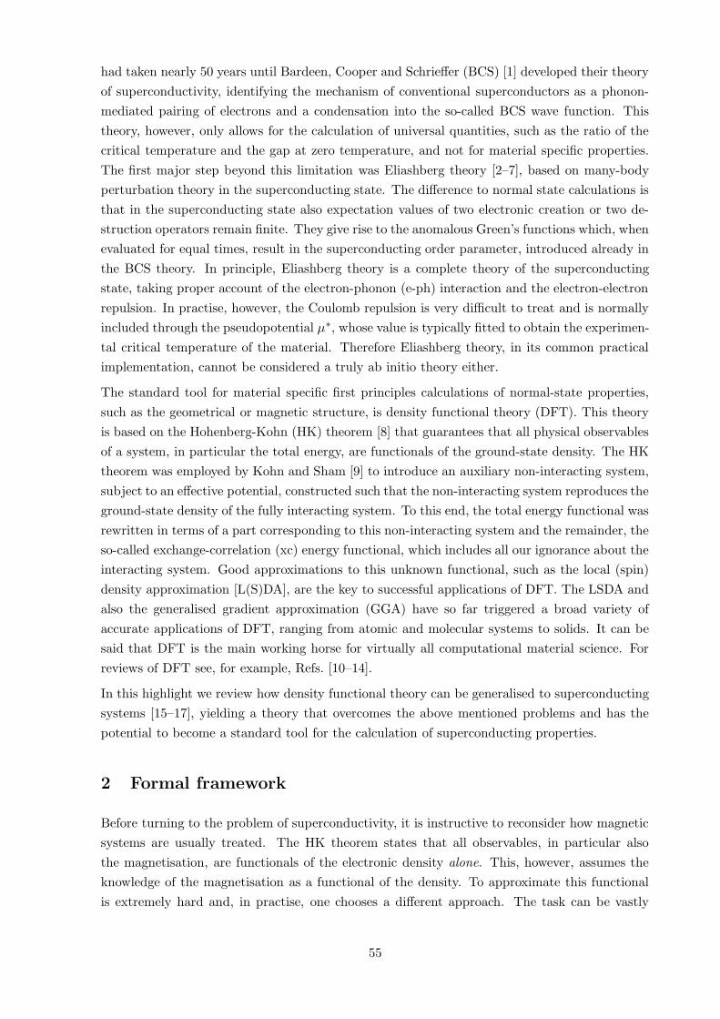
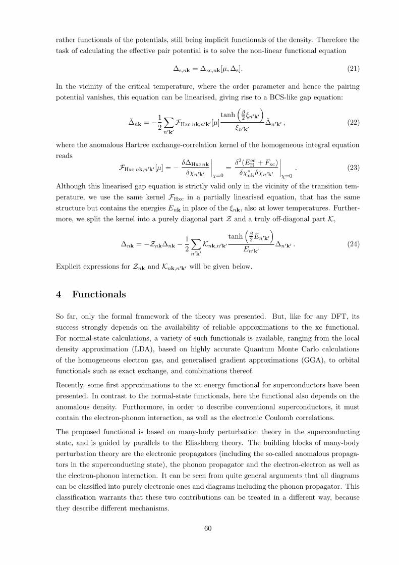
For the electron-phonon contributions an LDA-type functional is not meaningful, because the

homogeneous electron gas does not posses phonons. Instead, the e-ph contribution to the xc

energy is directly calculated from many-body perturbation theory by evaluating the two lowest

order diagrams, shown in Figure 1. The expressions for the xc energies can be found in Ref. [16].

a b

Figure 1: Lowest order phononic (a, b) contributions to Fxc. The two types of electron propa-

gators correspond to the normal and anomalous Green’s functions.

Besides the Coulomb repulsion and the electron-phonon coupling, spin-fluctuations constitute

another important mechanism. Ferromagnetic spin-fluctuations are known to lower the critical

temperature in materials such as vanadium and even to suppress superconductivity in palla-

dium, while antiferromagnetic spin-fluctuations are amongst the candidates for the mechanism

of the high-Tc superconductors. Spin fluctuations can be treated in a similar way to the electron-

phonon term by replacing the phonon-propagator in the diagrams by the spin-fluctuation prop-

agator. This has been proposed in the context of the Eliashberg theory [25, 26] and recently a

first approximation in the context of DFT for superconductors was constructed [27].

5 Potentials and kernels

The functionals described above are only implicit functionals of the densities. The desired

functional derivatives can nevertheless be evaluated by applying the chain rule of functional

derivatives, similar to the procedure used in the optimised effective potential method [28, 29].

The xc energy is an explicit functional of the pairing potential and the chemical potential, and

therefore we can write

∆xc nk = −δFxc

δµ

δµ

δχ∗nk

−∑

n′k′

[

δFxc

δ|∆n′k′ |2δ|∆n′k′ |2

δχ∗nk

+δFxc

δ(φn′k′)

δ(φn′k′)

δχ∗nk

]

. (25)

The partial derivatives of Fxc can be calculated directly. The remaining functional derivatives

are somewhat harder to obtain, but can be derived from the definitions of the densities, Eqs. (20),

61

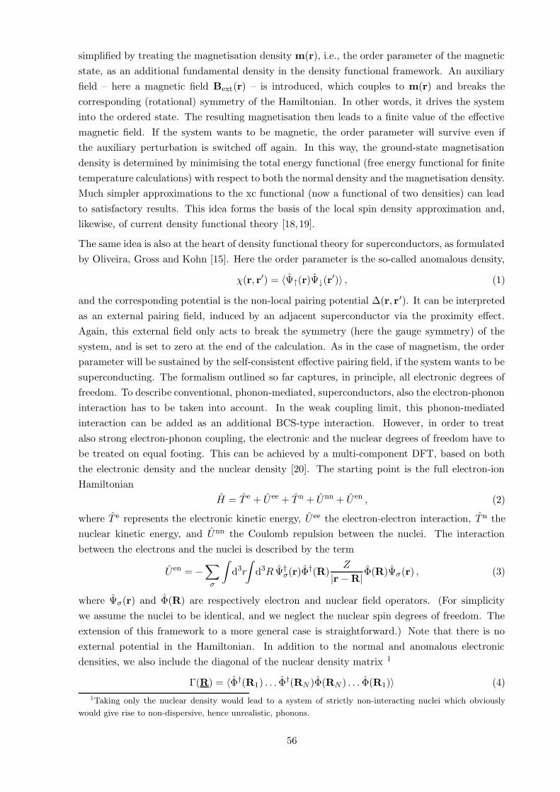
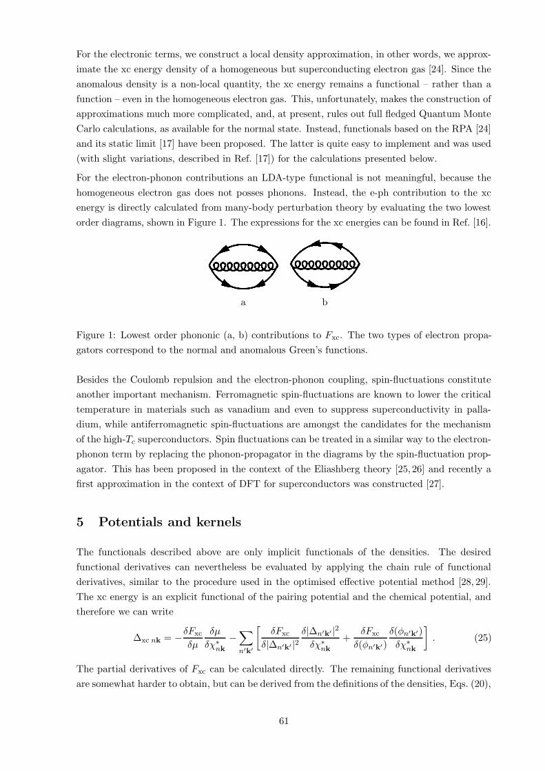
Table 1: Critical temperature (left panel) and superconducting gap at Fermi level and T = 0.01 K

(right panel), compared with experiment [30]. We also show the total electron-phonon coupling

constant λ [31, 32]. While TF-ME represents an approximation with the full matrix elements,

TF-SK and TF-FE correspond to simplified expressions. For details see Ref. [17].

Tc [K]

TF-ME TF-SK TF-FE exp λ

Mo — 0.33 0.54 0.92 0.42

Al 0.90 0.90 1.0 1.18 0.44

Ta 3.7 2.7 4.8 4.48 0.84

Pb 6.9 7.2 6.8 7.2 1.62

Nb 9.5 8.4 9.4 9.3 1.18

∆0 [meV]

TF-ME TF-SK TF-FE exp λ

Mo — 0.049 0.099 —- 0.42

Al 0.14 0.15 0.15 0.179 0.44

Ta 0.63 0.53 0.76 0.694 0.84

Pb 1.34 1.40 1.31 1.33 1.62

Nb 1.74 1.54 1.79 1.55 1.18

and from the fact that the particle density and the anomalous density are independent variables,

leading to the conditionδn(x)

δχ∗(r, r′)= 0 . (26)

After a number of further approximations (see [16,17]), the final expressions for the functionals

Znk and Knk,n′k′ in the gap equation (24) read as follows. There are two contributions stemming

from the electron-phonon interaction: i) The non-diagonal one is:

Kphnk,n′k′ =

2

tanh(

β2 ξnk

)

tanh(

β2 ξn′k′

)

×∑

λ,q

∣

∣

∣gnk,n′k′

λ,q

∣

∣

∣

2[I(ξnk, ξn′k′ ,Ωλ,q) − I(ξnk,−ξn′k′ ,Ωλ,q)] , (27)

where gnk,n′k′

λ,q are the electron-phonon coupling constants and the function I is defined as

I(ξ, ξ′,Ω) = fβ(ξ) fβ(ξ′)nβ(Ω)

[

eβξ − eβ(ξ′+Ω)

ξ − ξ′ − Ω− eβξ′ − eβ(ξ+Ω)

ξ − ξ′ + Ω

]

. (28)

In the previous expression fβ and nβ are the Fermi-Dirac and Bose-Einstein distributions; ii) The

second contribution is diagonal in nk and reads

Zphnk

=1

tanh(

β2 ξnk

)

∑

n′k′

∑

λ,q

∣

∣

∣gnk,n′k′

λ,q

∣

∣

∣

2[J(ξnk, ξn′k′ ,Ωλ,q) + J(ξnk,−ξn′k′ ,Ωλ,q)] , (29)

where the function J is defined by

J(ξ, ξ′,Ω) = J(ξ, ξ′,Ω) − J(ξ, ξ′,−Ω) , (30)

and we have

J(ξ, ξ′,Ω) = −fβ(ξ) + nβ(Ω)

ξ − ξ′ − Ω

[

fβ(ξ′) − fβ(ξ − Ω)

ξ − ξ′ − Ω− βfβ(ξ − Ω)fβ(−ξ′ + Ω)

]

. (31)

On the other hand, the Coulomb interaction leads to the term

KTF-MEnk,n′k′ = vTF

nk,n′k′ , (32)

62

0 2 4 6 8 10Experimental T

c [K]

0

2

4

6

8

10

Cal

cula

ted

Tc

[K]

Al

TF-METF-SKTF-FE

Ta

Pb Nb

Mo

0 0.5 1 1.5 2Experimental ∆

0 [meV]

0

0.5

1

1.5

2

Cal

cula

ted

∆ 0 [m

eV]

TF-METF-SKTF-FE

Al

TaPb

Nb

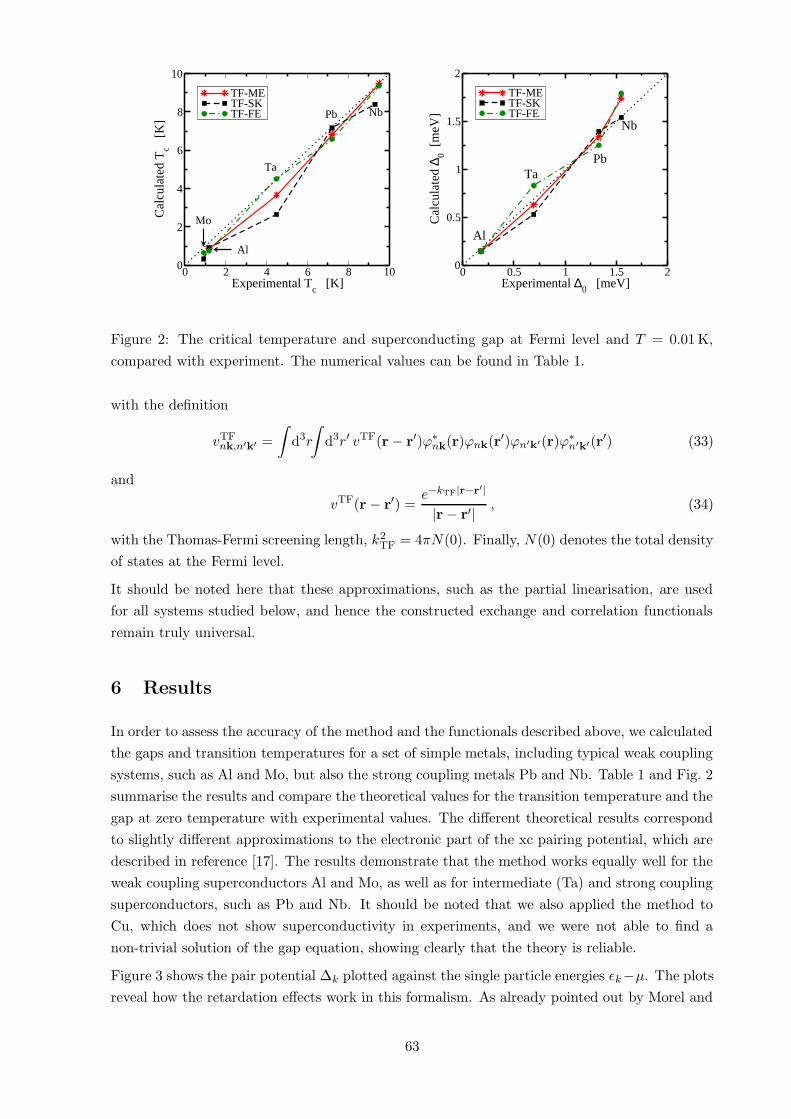
Figure 2: The critical temperature and superconducting gap at Fermi level and T = 0.01 K,

compared with experiment. The numerical values can be found in Table 1.

with the definition

vTFnk,n′k′ =

∫

d3r

∫

d3r′ vTF(r− r′)ϕ∗nk(r)ϕnk(r′)ϕn′k′(r)ϕ∗

n′k′(r′) (33)

and

vTF(r − r′) =e−kTF|r−r′|

|r − r′| , (34)

with the Thomas-Fermi screening length, k2TF = 4πN(0). Finally, N(0) denotes the total density

of states at the Fermi level.

It should be noted here that these approximations, such as the partial linearisation, are used

for all systems studied below, and hence the constructed exchange and correlation functionals

remain truly universal.

6 Results

In order to assess the accuracy of the method and the functionals described above, we calculated

the gaps and transition temperatures for a set of simple metals, including typical weak coupling

systems, such as Al and Mo, but also the strong coupling metals Pb and Nb. Table 1 and Fig. 2

summarise the results and compare the theoretical values for the transition temperature and the

gap at zero temperature with experimental values. The different theoretical results correspond

to slightly different approximations to the electronic part of the xc pairing potential, which are

described in reference [17]. The results demonstrate that the method works equally well for the

weak coupling superconductors Al and Mo, as well as for intermediate (Ta) and strong coupling

superconductors, such as Pb and Nb. It should be noted that we also applied the method to

Cu, which does not show superconductivity in experiments, and we were not able to find a

non-trivial solution of the gap equation, showing clearly that the theory is reliable.

Figure 3 shows the pair potential ∆k plotted against the single particle energies εk−µ. The plots

reveal how the retardation effects work in this formalism. As already pointed out by Morel and

63

0.0001 0.001 0.01 0.1 1 10ξ [eV]

-0.4

-0.2

0.0

0.2

0.4

0.6

0.8

1.0

1.2

1.4

∆ [

meV

]

ExperimentTF-ME, T = 0 KTF-SK, T = 0 KTF-SK, T = 6 KTF-SK, T = 7 K

Pb

0.0001 0.001 0.01 0.1 1 10 ξ [eV]

-0.8

-0.4

0.0

0.4

0.8

1.2

1.6

2.0

∆ [

meV

]

ExperimentTF-ME, T = 0 KTF-SK, T = 0 KTF-FE, T = 0 K

Nb

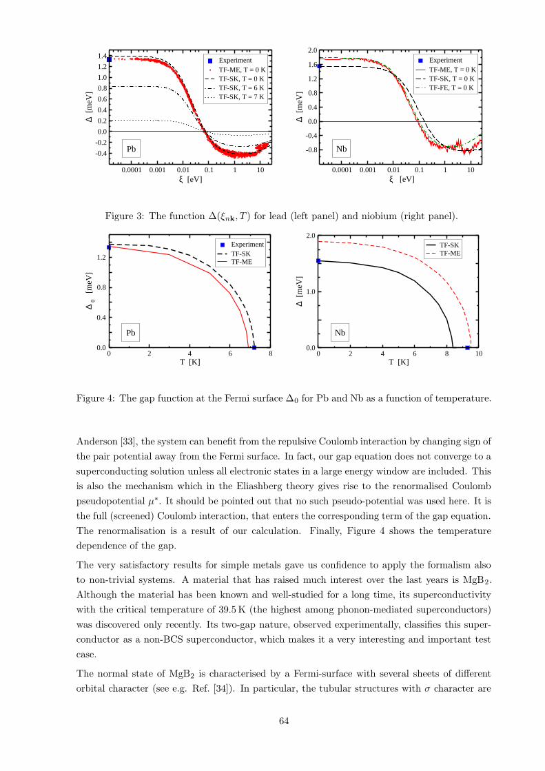
Figure 3: The function ∆(ξnk, T ) for lead (left panel) and niobium (right panel).

0 2 4 6 8T [K]

0.0

0.4

0.8

1.2

∆0

[meV

]

ExperimentTF-SKTF-ME

Pb

0 2 4 6 8 10T [K]

0.0

1.0

2.0

∆ [

meV

]

TF-SKTF-ME

Nb

Figure 4: The gap function at the Fermi surface ∆0 for Pb and Nb as a function of temperature.

Anderson [33], the system can benefit from the repulsive Coulomb interaction by changing sign of

the pair potential away from the Fermi surface. In fact, our gap equation does not converge to a

superconducting solution unless all electronic states in a large energy window are included. This

is also the mechanism which in the Eliashberg theory gives rise to the renormalised Coulomb

pseudopotential µ∗. It should be pointed out that no such pseudo-potential was used here. It is

the full (screened) Coulomb interaction, that enters the corresponding term of the gap equation.

The renormalisation is a result of our calculation. Finally, Figure 4 shows the temperature

dependence of the gap.

The very satisfactory results for simple metals gave us confidence to apply the formalism also

to non-trivial systems. A material that has raised much interest over the last years is MgB2.

Although the material has been known and well-studied for a long time, its superconductivity

with the critical temperature of 39.5 K (the highest among phonon-mediated superconductors)

was discovered only recently. Its two-gap nature, observed experimentally, classifies this super-

conductor as a non-BCS superconductor, which makes it a very interesting and important test

case.

The normal state of MgB2 is characterised by a Fermi-surface with several sheets of different

orbital character (see e.g. Ref. [34]). In particular, the tubular structures with σ character are

64

0.001 0.01 0.1 1 10 ε − µ [eV]

-2

0

2

4

6

8

∆ [

meV

]

σ σ Average π π AverageExperiments

π

AAAAAAAU

+

σ

JJ

JJ

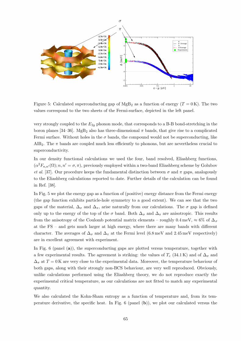
Figure 5: Calculated superconducting gap of MgB2 as a function of energy (T = 0 K). The two

values correspond to the two sheets of the Fermi-surface, depicted in the left panel.

very strongly coupled to the E2g phonon mode, that corresponds to a B-B bond-stretching in the

boron planes [34–36]. MgB2 also has three-dimensional π bands, that give rise to a complicated

Fermi surface. Without holes in the σ bands, the compound would not be superconducting, like

AlB2. The π bands are coupled much less efficiently to phonons, but are nevertheless crucial to

superconductivity.

In our density functional calculations we used the four, band resolved, Eliashberg functions,

(α2Fn,n′(Ω);n, n′ = σ, π), previously employed within a two-band Eliashberg scheme by Golubov

et al. [37]. Our procedure keeps the fundamental distinction between σ and π gaps, analogously

to the Eliashberg calculations reported to date. Further details of the calculation can be found

in Ref. [38].

In Fig. 5 we plot the energy gap as a function of (positive) energy distance from the Fermi energy

(the gap function exhibits particle-hole symmetry to a good extent). We can see that the two

gaps of the material, ∆σ and ∆π, arise naturally from our calculations. The σ gap is defined

only up to the energy of the top of the σ band. Both ∆σ and ∆π are anisotropic. This results

from the anisotropy of the Coulomb potential matrix elements – roughly 0.4 meV, ≈ 6% of ∆σ

at the FS – and gets much larger at high energy, where there are many bands with different

character. The averages of ∆σ and ∆π at the Fermi level (6.8 meV and 2.45 meV respectively)

are in excellent agreement with experiment.

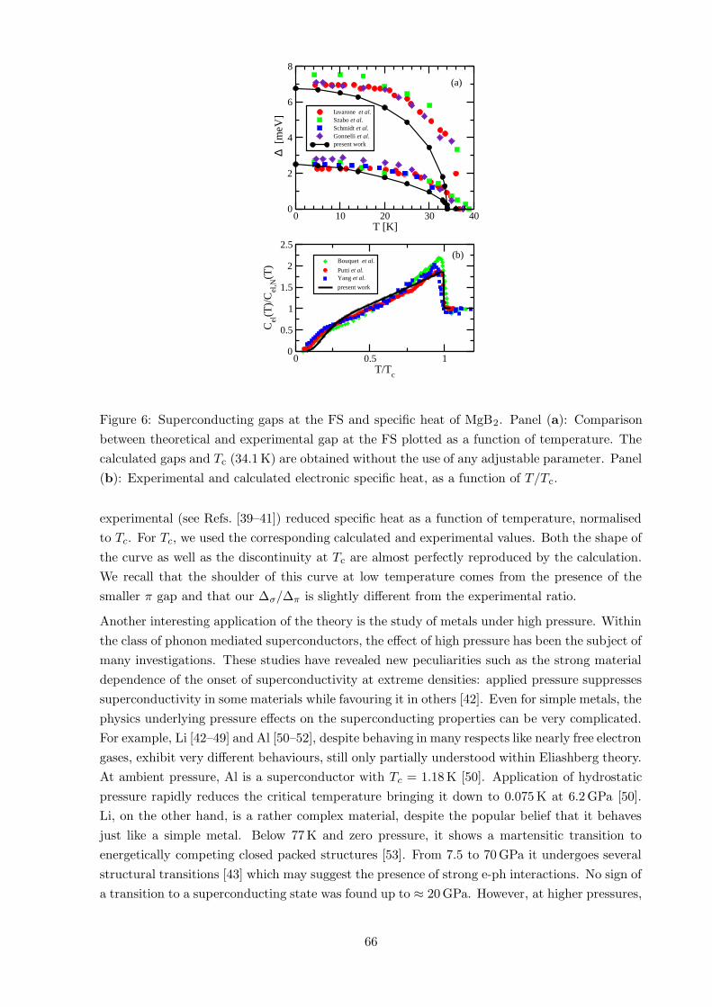
In Fig. 6 (panel (a)), the superconducting gaps are plotted versus temperature, together with

a few experimental results. The agreement is striking: the values of Tc (34.1 K) and of ∆σ and

∆π at T = 0 K are very close to the experimental data. Moreover, the temperature behaviour of

both gaps, along with their strongly non-BCS behaviour, are very well reproduced. Obviously,

unlike calculations performed using the Eliashberg theory, we do not reproduce exactly the

experimental critical temperature, as our calculations are not fitted to match any experimental

quantity.

We also calculated the Kohn-Sham entropy as a function of temperature and, from its tem-

perature derivative, the specific heat. In Fig. 6 (panel (b)), we plot our calculated versus the

65

0 10 20 30 40T [K]

0

2

4

6

8

∆ [

meV

] Iavarone et al.Szabo et al.Schmidt et al.Gonnelli et al.present work

0 0.5 1T/T

c

0

0.5

1

1.5

2

2.5

Cel

(T)/

Cel

,N(T

)Bouquet et al.

Putti et al.Yang et al.

present work

(a)

(b)

Figure 6: Superconducting gaps at the FS and specific heat of MgB2. Panel (a): Comparison

between theoretical and experimental gap at the FS plotted as a function of temperature. The

calculated gaps and Tc (34.1 K) are obtained without the use of any adjustable parameter. Panel

(b): Experimental and calculated electronic specific heat, as a function of T/Tc.

experimental (see Refs. [39–41]) reduced specific heat as a function of temperature, normalised

to Tc. For Tc, we used the corresponding calculated and experimental values. Both the shape of

the curve as well as the discontinuity at Tc are almost perfectly reproduced by the calculation.

We recall that the shoulder of this curve at low temperature comes from the presence of the

smaller π gap and that our ∆σ/∆π is slightly different from the experimental ratio.

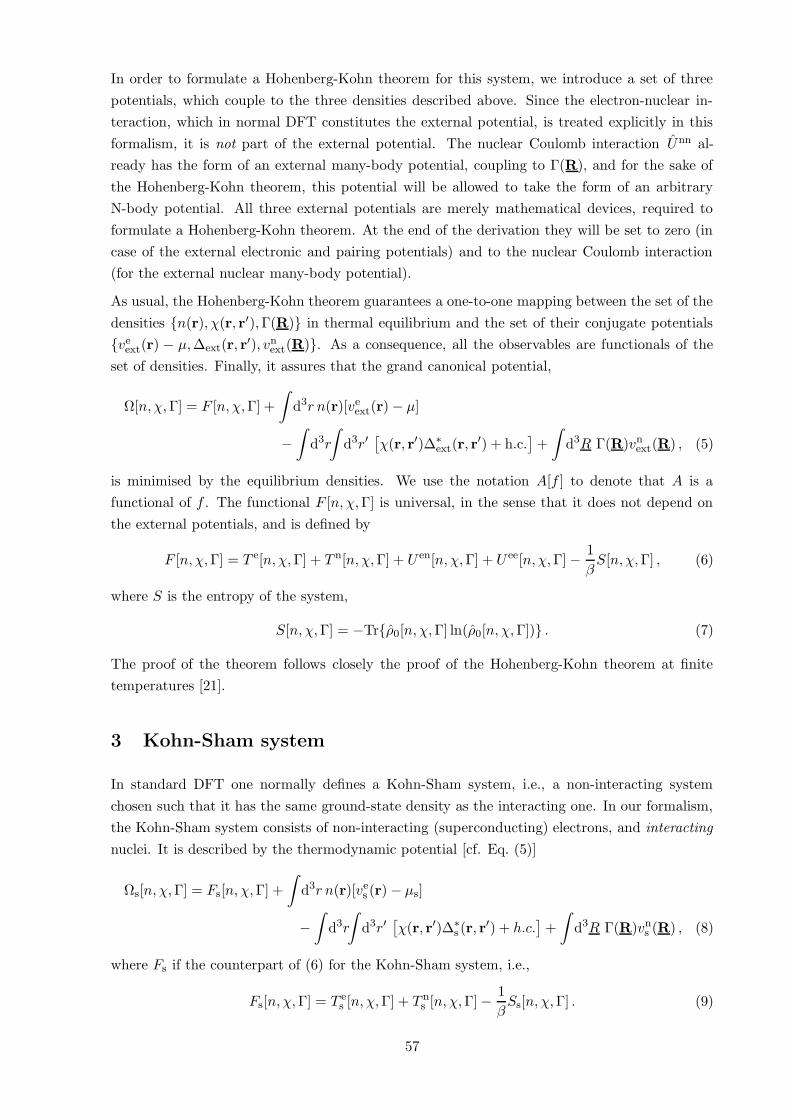
Another interesting application of the theory is the study of metals under high pressure. Within

the class of phonon mediated superconductors, the effect of high pressure has been the subject of

many investigations. These studies have revealed new peculiarities such as the strong material

dependence of the onset of superconductivity at extreme densities: applied pressure suppresses

superconductivity in some materials while favouring it in others [42]. Even for simple metals, the

physics underlying pressure effects on the superconducting properties can be very complicated.

For example, Li [42–49] and Al [50–52], despite behaving in many respects like nearly free electron

gases, exhibit very different behaviours, still only partially understood within Eliashberg theory.

At ambient pressure, Al is a superconductor with Tc = 1.18 K [50]. Application of hydrostatic

pressure rapidly reduces the critical temperature bringing it down to 0.075 K at 6.2 GPa [50].

Li, on the other hand, is a rather complex material, despite the popular belief that it behaves

just like a simple metal. Below 77 K and zero pressure, it shows a martensitic transition to

energetically competing closed packed structures [53]. From 7.5 to 70 GPa it undergoes several

structural transitions [43] which may suggest the presence of strong e-ph interactions. No sign of

a transition to a superconducting state was found up to ≈ 20 GPa. However, at higher pressures,

66

2 4 6 8 10 12 14 16ω(THz)

0.1

0.2

0.3

0.4

0.5

0.6

0.7

α2 F

36.9 22.5 8.5 4.5 0.2

Al

0 1 2 3 4 5 6 7Pressure (GPa)

0

0.5

1

1.5

Tc (

K)

SCDFTMcMillan (0.13)Gubser [44]Sundqvist [45]

0 5 10 15 20ω(THz)

0

0.2

0.4

0.6

0.8

α2 F

3529.722.313100

Li

0 20 40 60 80Pressure (GPa)

0

5

10

15

20

Tc (

K)

fcc

hR1

cI16

LinShimizuStruzhkinDeemyadMcMillan (0.22)SCDFTMcMillan (0.13)

0 1 2 3 4 5 6ω(THz)

0

0.5

1

1.5

α2 F

28.822.70

K

20 22 24 26 28Pressure (GPa)

0

5

10

15

Tc (

K)

SCDFTMcMillan (µ* = 0.11)McMillan (µ* = 0.23)

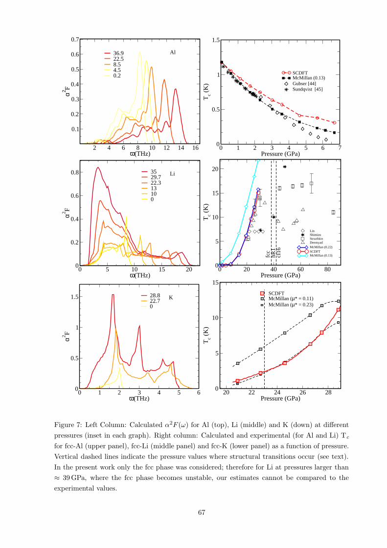
Figure 7: Left Column: Calculated α2F (ω) for Al (top), Li (middle) and K (down) at different

pressures (inset in each graph). Right column: Calculated and experimental (for Al and Li) Tc

for fcc-Al (upper panel), fcc-Li (middle panel) and fcc-K (lower panel) as a function of pressure.

Vertical dashed lines indicate the pressure values where structural transitions occur (see text).

In the present work only the fcc phase was considered; therefore for Li at pressures larger than

≈ 39 GPa, where the fcc phase becomes unstable, our estimates cannot be compared to the

experimental values.

67

Li becomes a superconductor [44–47]. In the range 20-38.3 GPa, where Li crystalizes in an fcc

structure, experiments by Shimizu [45], Struzhkin [46], and Deemyad [47] found that Tc increases

rapidly with pressure, reaching values around 12–17 K (one of the highest Tc observed so far

in any elemental superconductor). However, experiments report different behaviours and quite

large deviations.

In Fig. 7 we show the calculated pressure dependence of Tc for Al (upper panel), Li (middle

panel), and K (lower panel), compared with experimental results. (Details about the calculations

can be found in Refs. [54,55].) For Al, the calculated zero pressure Tc =1.18 K matches exactly

the experimental value.2 Upon compression, the calculation reproduces quite well the rapid

decrease of Tc. A reduction by a factor of 10 with respect to the zero-pressure value is obtained

at a pressure (' 8.5 GPa) slightly higher than experiment (6.2 GPa). Similar theoretical results

are obtained within the standard McMillan formula [56] (open circles in Fig. 7) using µ∗=0.13

in agreement with previous calculations [52]. The small values of Tc in this pressure range make

it quite difficult to extract a good estimate, from both experiments and theory. Nevertheless,

the calculations show the asymptotic saturation of Tc rather than the linear decay suggested

by experimental data. This discrepancy (with the only experiment available) calls for further

experimental investigations in this pressure range.

In the middle panel of Fig. 7 we report the available experiments for Li compared with our

calculated values. In the pressure range from 20 to 35 GPa, where the newer experiments [46,47]

are in agreement and show a clear increase of Tc with increasing pressure, our calculated results

reproduce the experimental trend of Tc and sit close to the experimental values. The calculated

pressure which determines the onset of the superconducting state is about 10 GPa, where we

predict Tc ≈ 0.2 K. This finding agrees with Deemyad and Schilling [47], who claim that no

superconducting transition above 4 K exists below 20 GPa. Our result is in good agreement

with the highest measured Tc, 14 K [47], 16 K [46] and 17 K [45], and improves significantly

upon the theoretical estimates by Christensen et al. [48], who discussed a paramagnon (i.e., spin

fluctuations) dependent Tc varying between 45 and 75 K.

Due to the first principles nature of the method, it is feasible to make predictions on unknown

superconductors: we apply the method to find a possible superconducting instability in potas-

sium under pressure. Fcc-K shows a behaviour quite similar to Li: beyond a pressure threshold

(20 GPa) Tc rises rapidly. In the range where phonons were found to be stable, it reaches ∼11 K; the experimentally observed instability of the fcc phase, however, limits this value to ∼2 K.

We relate the appearance of superconductivity in Li and K to an incipient phase transition,

which gives rise to phonon softening and very strong electron-phonon coupling, that then leads

to the unusually high transition temperatures. In addition, our calculations for Li and K confirm

that a full treatment of electronic and phononic energy scales is required, which is in agreement

with previous arguments by Richardson and Ashcroft [57].

The different behaviour of Al on one side and Li and K on the other can be understood by

analysing the Eliashberg function as a function of pressure (see Fig. 7). In Al, the phonon

2This value is slightly different from the ones reported in Table 1, where the e-ph λ included was taken from

Ref. [32]. More details are given in Ref. [54].

68

frequencies increase as the pressure rises, corresponding to the normal stiffening of phonons

with increasing pressure. In addition, the height of the peaks in the Eliashberg spectral function

α2F (Ω) decreases with increasing pressure. These factors contribute to a decrease of the overall

coupling constant λ and, consequently, of the critical temperature Tc.

For alkali metals the situation is completely different: due to the incipient phase transitions, a

phonon softening at low frequencies increases the value of λ in both materials. However, the

different topology of the Fermi surfaces and the different range of the phonon frequencies sets

the critical temperature much higher in lithium with respect to potassium. For more details see

Ref. [54, 55]

7 Conclusion

We have developed a truly ab-initio approach to superconductivity without any adjustable pa-

rameters. The key feature is that the electron-phonon interaction and the Coulombic electron-

electron repulsion are treated on the same footing. This is achieved within a density-functional

framework, based on three “densities”: the ordinary electronic density, the superconducting

order parameter, and the diagonal of the nuclear N -body density matrix. The formalism leads

to a set of Kohn-Sham equations for the electrons and the nuclei. The electronic Kohn-Sham

equations have the structure of Bogoliubov-de Gennes equations but, in contrast to the latter,

they incorporate normal and anomalous xc potentials. Likewise, the Kohn-Sham equation de-

scribing the nuclear motion contains, besides the bare nuclear Coulomb repulsion, an exchange-

correlation interaction.

The exchange-correlation potentials are functional derivatives of a universal functional Fxc[n, χ,Γ]

that represents the exchange-correlation part of the free energy. Approximations for this func-

tional were then derived by many-body perturbation theory. To this end, the effective nuclear

interaction was expanded to second order in the displacements from the nuclear equilibrium

positions. By introducing the usual collective (phonon) coordinates, the nuclear Kohn-Sham

equation is then transformed into a set of harmonic oscillator equations describing independent

phonons. These non-interacting phonons, together with non-interacting but superconducting

(Kohn-Sham) electrons serve as unperturbed system for a Gorling-Levy-type perturbative ex-

pansion [58] of Fxc. The electron-phonon interaction and the bare electronic Coulomb repulsion,

as well as some residual exchange-correlation potentials, are treated as the perturbation. In this

way, both Coulombic and electron-phonon couplings are fully incorporated.

The solution of the KS-Bogoliubov-de Gennes equation (or the KS gap equation together with the

normal-state Schrodinger equation) fully determines the Kohn-Sham system. Therefore, within

the usual approximation to calculate observables from the Kohn-Sham system, one can apply the

full variety of expressions for physical quantities, known from phenomenological Bogoliubov-de

Gennes theory, also in the present framework.

Superconducting properties of simple conventional superconductors have been computed with-

out any experimental input. In this way, we were able to test the theory and to assess the

quality of the functionals proposed. The most important result is that the calculated transition

temperatures and superconducting gaps are in good agreement with experimental values. The

69

largest deviations from the experimental results are found for the elements in the weak coupling

limit with Mo being the most pronounced example. We also calculated the isotope effect for Mo

and Pb (see Ref. [17]), achieving again rather good agreement with experiment. These results

clearly show that retardation effects are correctly described by the theory.

For MgB2 we obtained the value of Tc, the two gaps, as well as the specific heat as a function

of temperature in very good agreement with experiment. We stress the predictive power of the

approach presented: Being, by its very nature, a fully ab-initio approach, it does not require

semi-phenomenological parameters, such as µ∗. Nevertheless, it is able to reproduce with good

accuracy superconducting properties, previously out of reach of first-principles calculations.

Finally, we also calculated the superconducting transition temperature of Al, K and Li under

high pressure from first principles. The results obtained for Al and Li are in very good agreement

with experiment, and account for the opposite behaviour of these two metals under pressure.

Furthermore, the increase of Tc with pressure in Li is explained in terms of the strong e-ph

coupling, which is due to changes in the topology of the Fermi surface, and is responsible for

the observed structural instability. Finally, our results for fcc-K provide predictions interesting

enough to suggest experimental work on this system.

References

[1] J. Bardeen, L. N. Cooper, and J. R. Schrieffer, Phys. Rev. 108, 1175 (1957).

[2] G. M. Eliashberg, Sov. Phys. JETP 11, 696 (1960).

[3] D. J. Scalapino, J. R. Schrieffer, and J. W. Wilkins, Phys. Rev. 148, 263 (1966).

[4] J. R. Schrieffer, Theory of Superconductivity, Vol. 20 of Frontiers in Physics (Addison-

Wesley, Reading, 1964).

[5] D. J. Scalapino, in Superconductivity, edited by R. D. Parks (Marcel Dekker, New York,

1969), Vol. 1, Chap. 10, p. 449.

[6] P. B. Allen and B. Mitrovic, Solid State Physics, edited by F. Seitz (Academic Press, Inc.,

New York, 1982), Vol. 37, p. 1.

[7] J. P. Carbotte, Rev. Mod. Phys. 62, 1027 (1990).

[8] P. Hohenberg and W. Kohn, Phys. Rev. 136, B864 (1964).

[9] W. Kohn and L.J. Sham, Phys. Rev. 140, A1133 (1965).

[10] R.M. Dreizler and E.K.U. Gross, Density Functional Theory (Springer, Berlin, 1990).

[11] H. Eschrig, The Fundamentals of Density Functional Theory, Vol. 32 of Teubner-Texte zur

Physik (B. G. Teubner Verlagsgesellschaft, Stuttgart-Leipzig, 1996).

[12] Density Functional Theory, Vol. 337 of NATO ASI Series B, edited by E.K.U. Gross and

R.M. Dreizler (Plenum Press, New York, 1995).

70

[13] A Primer in Density Functional Theory, Vol. 620 of Lecture Notes in Physics, edited by C.

Fiolhais, F. Nogueira, and M. Marques (Springer, 2003).

[14] R. O. Jones and O. Gunnarsson, Rev. Mod. Phys. 61, 689 (1989).

[15] L. N. Oliveira, E. K. U. Gross, and W. Kohn, Phys. Rev. Lett. 60, 2430 (1988).

[16] M. Luders, M. A. L. Marques, N. N. Lathiotakis, A. Floris, G. Profeta, L. Fast, A. Conti-

nenza, S. Massidda, and E. K. U. Gross, Phys. Rev. B 72, 024545 (2005).

[17] M. A. L. Marques, M. Luders, N. N. Lathiotakis, G. Profeta, A. Floris, L. Fast, A. Conti-

nenza, E. K. U. Gross, and S. Massidda, Phys. Rev. B 72, 024546 (2005).

[18] G. Vignale and Mark Rasolt, Phys. Rev. Lett. 59, 2360 (1987).

[19] G. Vignale and Mark Rasolt, Phys. Rev. B 37, 10685 (1988).

[20] T. Kreibich and E. K. U. Gross, Phys. Rev. Lett. 86, 2984 (2001).

[21] N. D. Mermin, Phys. Rev. 137, A1441 (1965).

[22] N. N. Bogoliubov, Sov. Phys. JETP 7, 41 (1958).

[23] E. K. U. Gross and Stefan Kurth, Int. J. Quantum Chem. Symp. 25, 289 (1991).

[24] S. Kurth, M. Marques, M. Luders, and E. K. U. Gross, Phys. Rev. Lett. 83, 2628 (1999).

[25] H. Rietschel and H. Winter, Phys. Rev. Lett. 43, 1256 (1979).

[26] R. C. Zehder and H. Winter, J.Phys.: Condens. Matter 2, 7479 (1990).

[27] M. Wierzbowska, Eur. Phys. J. B 48, 207 (2005).

[28] T. Grabo, T. Kreibich, S. Kurth, and E. K. U. Gross, in Strong Coulomb Correlations in

Electronic Structure Calculations: Beyond the Local Density Approximation, edited by V. I.

Anisimov (Gordon and Breach, 2000), pp. 203 – 311.

[29] T. Grabo, E.K.U. Gross, and M. Luders, Orbital Functionals in Density Functional Theory:

The Optimized Effective Potential Method, Highlight of the month in Psi-k Newsletter 16,

1996.

[30] N. W. Ashcroft and N. D. Mermin, Solid State Physics (Saunders College Publishing, Fort

Worth, 1976).

[31] S. Yu. Savrasov, Phys. Rev. Lett. 69, 2819 (1992).

[32] S. Y. Savrasov and D. Y. Savrasov, Phys. Rev. B 54, 16487 (1996).

[33] P. Morel and P. W. Anderson, Phys. Rev. 125, 1263 (1962).

[34] J. Kortus, I. I. Mazin, K. D. Belashchenko, V. P. Antropov, and L. L. Boyer, Phys. Rev. Lett.

86, 4656 (2001).

[35] J. M. An and W. E. Pickett, Phys. Rev. Lett. 86, 4366 (2001).

71

[36] Y. Kong, O. V. Dolgov, O. Jepsen, and O. K. Andersen, Phys. Rev. B 64, 020501 (2001).

[37] A. A. Golubov, J. Kortus, O. V. Dolgov, O. Jepsen, Y. Kong, O. K. Andersen, B. J. Gibson,

K. Ahn, and R. K. Kremer, J. Phys.: Condens. Matter 14, 1353 (2002).

[38] A. Floris, G. Profeta, N. N. Lathiotakis M. Luders, M. A. L. Marques, C. Franchini, E. K. U.

Gross, A. Continenza, and S. Massidda, Phys. Rev. Lett. 94, 037004 (2005).

[39] M. Putti, M. Affronte, P. Manfrinetti, and A. Palenzona, Phys. Rev. B 68, 094514 (2003).

[40] F. Bouquet, R. A. Fisher, N. E. Phillips, D. G. Hinks, and J. D. Jorgensen, Phys. Rev. Lett.

87, 47001 (2001).

[41] H. D. Yang, J.-Y. Lin, H. H. Li, F. H. Hsu, C. J. Liu, S.-C. Li, R.-C. Yu, and C.-Q. Jin,

Phys. Rev. Lett. 87, 167003 (2001).

[42] N. W. Ashcroft, Nature 419, 569 (2002).

[43] M. Hanfland, K. Syassen, N. E. Christensen, and D. L. Novikov, Nature 408, 174 (2000).

[44] T. H. Lin and K. J. Dunn, Phys. Rev. B 33, 807 (1986).

[45] K. Shimizu, H. Ishikawa, D. Takao, T. Yagi, and K. Amaya, Nature 419, 597 (2002).

[46] V. V. Struzhkin, M. I. Eremets, W. Gan, H.-K. Mao, and R. J. Hemley, Science 298, 1213

(2002).

[47] S. Deemyad and J. S. Schilling, Phys. Rev. Lett. 91, 167001 (2003).

[48] N. E. Christensen and D. L. Novikov, Phys. Rev. Lett. 86, 1861 (2001).

[49] J. B. Neaton and N. W. Ashcroft, Nature 400, 141 (1999).

[50] D. U. Gubser and A. W. Webb, Phys. Rev. Lett. 35, 104 (1975).

[51] B. Sundqvist and O. Rapp, J. Phys. F: Metal Phys. 79, L161 (1979).

[52] M. L. Cohen M. M. Dacorogna and P. K. Lam, Phys. Rev. B 34, 4865 (1986).

[53] V. G. Vaks, M. I. Katsnelson, V. G. Koreshkov, A. I. Likhtenstein, O. E. Parfenov, V. F.

Skok, V. A. Sukhoparov, A. V. Trefilov, and A. A. Chernyshov, J. Phys.: Condens. Matter

1, 5319 (1998).

[54] G. Profeta, C. Franchini, N. N. Lathiotakis, A. Floris, A. Sanna, M. A. L. Marques, M.

Luders, S. Massidda, E. K. U. Gross, and A. Continenza, Phys. Rev. Lett. 96, 047003

(2006).

[55] A. Sanna, C. Franchini, A. Floris, G. Profeta, N. N. Lathiotakis, M. Luders, M. A. L.

Marques, E. K. U. Gross, A. Continenza, and S. Massidda, Phys. Rev. B 73, 144512

(2006).

[56] W. L. McMillan, Phys. Rev. 167, 331 (1968).

72

[57] C. F. Richardson and N. W. Ashcroft, Phys. Rev. B 55, 15130 (1997).

[58] A. Gorling and M. Levy, Phys. Rev. A 50, 196 (1994).

73