Préparée à Chimie ParisTech Density-based approaches to photo-induced properties and reactivity of molecular systems Soutenue par Federica Maschietto Le 21 octobre 2019 Ecole doctorale n° 388 Chimie Physique et Chimie Analytique de Paris-Centre Spécialité Chimie physique Composition du jury : Esmail, ALIKHANI Professeur, Sorbonne Université Président Masahiro, EHARA Professor, Institute for Molecular Science Rapporteur Nadia, REGA Professor, Università degli Studi di Napoli Rapporteur Victor S., BATISTA John Randolph Huffman Professor of Chemistry, Yale University Examinateur Ilaria, CIOFINI Directrice de recherche, Chimie ParisTech Directrice de thèse

Welcome message from author
This document is posted to help you gain knowledge. Please leave a comment to let me know what you think about it! Share it to your friends and learn new things together.
Transcript
Préparée à Chimie ParisTech
Density-based approaches to photo-induced properties and reactivity of molecular systems
Soutenue par Federica Maschietto Le 21 octobre 2019
Ecole doctorale n° 388 Chimie Physique et Chimie Analytique de Paris-Centre
Spécialité Chimie physique
Composition du jury : Esmail, ALIKHANI Professeur, Sorbonne Université Président
Masahiro, EHARA Professor, Institute for Molecular Science Rapporteur
Nadia, REGA Professor, Università degli Studi di Napoli Rapporteur
Victor S., BATISTA John Randolph Huffman Professor of Chemistry, Yale University Examinateur
Ilaria, CIOFINI Directrice de recherche, Chimie ParisTech Directrice de thèse


ACKNOWLEDGMENTS
I am thankful for so much in this three-year cycle, I (at least) owe a debt of gratitudeto all those I had the privilege to work alongside. Each has contributed considerably toenrich this time and their thoughts and suggestions have been essential. I want to takethe chance to you all here.
I first must express my gratitude to my phD advisor, Ilaria Ciofini, to whom I am deeplygrateful for the constant scientific, but also human support she has offered me duringthese years. Having a mentor is a privilege, especially as you are to me a brilliant exampleof how a professional scientist should think and work. I will always be grateful to you forthe many advises and constructive critics you have addressed to me.
If it is true, as I believe, that each is the fruit of the environment in which it grows I canonly address my thanks to Carlo Adamo - director of the department I have been workingin. Thank you for for sharing your knowledge and expertise, as well as your memorablestories, unavoidable side-dish of every day’s lunch.
My gratitude goes also to Frederic Labat, who, besides sharing his office with me, alwaysmade his knowledge and expertise available.
Thanks are given also to those who have kindly accepted to be members of the jury: EsmailAlikhani, Victor Batista, Masahiro Ehara and Nadia Rega.
My sincere thanks go to my near-office-friend Alistar Ottochian who did not miss onesingle occasion to prove its kindness and will to help, always prompt to take up a challengeand propose one.
Special thanks are also due to Liam Wilbraham and Pierpaolo Poier, sharp minds and andgood friends, with whom I had the pleasure to share - and I hope I will continue sharing -long discussions, both science related and not.
I have enormous gratitude for all my colleagues and friends for making Chimie Paris-Tech such an enjoyable environment, each with his/her peculiar character and mind. Inpseudo-chronological order of appearance Chiara Ricca, Alexandra Szemjonov, StefaniaDi Tommaso, Davide Presti, Anna Notaro, Franz Heinemann, Johannes Karges, MartaAlberto, Marco Campetella, Juan Sanz-Garcia, Indira Fabre, Luca Perego, Gloria Mazzone,Laura Le Bras, Eleonora Menicacci, Umberto Raucci, Francesco Muniz Miranda, Anna Per-fetto, Carmen Morgillo, Davide Luise, Jun Su, Bernardino Tirri, Dario Vassetti, GabriellyMiyazaki, Laure Thieulloy. I extend the thanks also to the excellent collaborators I havehad the pleasure to discuss and work with throughout this thesis, Aurelie Perrier, GillesGasser, Gilles Lemercier, Eric Brémond and Peter Reinhardt.
Big thanks to all friends at ENS, who have welcomed me in their environment in multipleoccasion, and without whom all unconventional (but pleasant) working hours would havenot even been imaginable.
3

4
Thanks to all friends in Paris, brothers-in-phD, who have shared with me this wonderfulexperience. You have enriched the last three years with you presence and wonderfulcompany.A warm acknowledgement goes to my four lovely friends Valentina Santolini, BlancheLacoste, Lia Bruna and Giulia Cosentino and to my sister Vittoria, for this occasion, allexceptional proofreaders. Although you are now living far, you never miss an occasion tooffer your support. You couldn’t be more effective and delightfully persistent, and I thankyou for this.A huge thanks goes to my parents, undefeatable optimists and most convinced supportersof my life challenges and career. An additional thank is due to my father for the "specialedition" my PhD thesis. This manuscript is the third title of a trilogy, which encloses thefinal writings of my cursus studiorum, including bachelor, master and finally doctoralthesis. Even if completely out of the usual themes of the MaschiettoEditore publishinghouse, you have proudly included all volumes in your catalog. Grazie Papà.Finally, I would like to dedicate a word to my life partner and true lifeblood Lorenzo,who in these three years, and with timeless conviction, has always been ready to offer mehis support. Your unwavering trust and unconditional tenderness have strengthened meevery day and enlightened each step of this three-year journey. You have given me hopeand courage for the future, and for that I will always be grateful to you.
5
abstract
The recent developments in theoretical photochemistry have proven the capability oftheoretical methods to provide solutions for an in-depth characterization of the photo-chemical properties and reactivity of organic and inorganic chromophores. In particular,time-dependent functional methods are nowadays considered amongst the most reliableand cost-effective computational tools to investigate excited state processes, and have con-tributed to confer theory a leading position in assisting new discoveries through rationalphotosynthetic design.
However, the results of these theoretical methodologies are often hard to interpret ona chemical basis, as an accurate description of the modeled system requires handling alarge set of output mathematical objects such as density matrices and orbital coefficients.
This thesis focuses on devising, constructing, and applying cost-effective approachesto calculate the photophysical properties of molecular systems in the context of densityfunctional theory. The objective of our work is to define a set of purposely-derived densitydescriptors that can be combined to provide a straightforward interpretation of therelevant photophysical pathways for the many processes taking place at the excited state.More specifically, we deliver a collection of TDDFT-based computational protocols, basedon the knowledge of ground and excited state densities, to characterize the excited-statepotential energy surfaces of molecular systems.In the first part of this manuscript, which comprises Chapter 2 and 3, we provide abrief introduction of the theoretical background and state of the art that motivates ourdevelopments.
The second part is dedicated to a systematic assessment of the DCT index [1], that is,an established metric that measures the extent of charge separation that results fromthe hole/particle generation of the excited state. This descriptor is the key componentof our methodology and lays the foundations for our developments. In Chapter 4, wesystematically analyze how the DCT index is affected by the density relaxation involved inthe post-linear response treatment of time-dependent density functional theory. For thispurpose, we consider a family of push-pull dyes of increasing length, where the primaryhole/particle charge-separation distance grows with the length of the molecular skeleton.First, we benchmark the influence of different density functional approximations on thisdescriptor, showing that it might yield considerably-different representations dependingon the kernel used for generating the exciton. Then, starting from this evidence, we theninvestigate the effect of relaxed and unrelaxed densities, showing that they both yielda consistent qualitative assessment of the nature of the excited states. In Chapter 5, wefurther benchmark the DCT index for retrieving the nature of excited states along a fullreaction. Using a prototype excited-state proton transfer reaction as a test case, we showthat the DCT and other density-based descriptors can be safely used for a quantitativeand qualitative assessment of excited states along the full photochemical process. Moreprecisely, the DCT provides a good description of the occurring electronic rearrangementsboth using density functional and multiconfigurational methods - here CASSCF-CASPT.We then discuss how the DCT could be employed, as it is usually done with energy
6
gradients, to locate minima on potential surfaces. In Chapter 6, we complement out theinvestigation with a diagnostic analysis probing the accuracy of TDDFT methods. Here,we rationalize what the pitfalls of TDDFT are, what is the reason for their appearanceand under what circumstances existing approximations work well or fail. The applicationof the MAC diagnostic analysis on different organic chromophores allows us to identifyghost- and spurious-low-lying excitations that result from a chosen density functionalapproximation. Furthermore, in Chapter 7, we extend such analysis to probe singlet andtriplet excitations in metal-containing complexes.
The third part is dedicated to the exploration of the excited state landscapes andrelaxation pathways, based on the density arguments. In Chapter 8, we extend our com-putational setup to characterize excited-state pathways in the case of reactions involving aprofound structural change. This investigation fits in the broader context of the computer-assisted design of new molecular architectures with peculiar photochemical traits, able forinstance, to store energy through reversible conformational changes induced by electronicexcitations. In particular, we extend the formulation of the index Π [2] to the charac-terization of potential energy surfaces of the lowest-lying excited states away from theFranck-Condon region, for instance, in regions involved in radiative and non-radiativedecay patterns.
Finally, in Chapter 9 we introduce a novel methodology aimed at tracking the nature ofelectronic states along the nuclear trajectory. This approach is based on the definition of astate-specific fingerprint that leverages the full information contained in the transitionvectors to give a unique characterization to any excited state of interest. We benchmarkthis method on three known photochemical reactions and show that it is able to preciselyrecover the nature of the excited state at each step of the reaction, for all systems.
Overall, the state-tracking algorithm and the density-descriptors outlined in this thesiscollectively provide a reliable and cost-effective way of disclosing excited state pathwayswithin the theoretical modeling of photophysical processes. The proposed approach can becomputed "on the fly" to identify critical areas for TDDFT approaches while, contextually,providing a method for the qualitative identification - in conjunction with energy criteria- of possible reactions paths.
PUBL ICAT IONS
This manuscript comprises the research work I have carried during my graduate studies inthe group of Chimie Théorique et Modélisation of École Nationale Superieure de ChimieParis, under the supervision of prof. Ilaria Ciofini, and includes a number of published aswell as original results.
A consistent part of my graduate research work has been dedicated to the development ofcomputational protocols, rooted on time-dependent density functional theory (TDDFT),aimed at the description of excited state processes at a molecular level. In particular, thisproject focused on the design and benchmark of a computational setup that makes useof purposely-developed density indexes to efficiently explore and describe the evolutionof excited states far from the Franck Condon region. Results from this line of work arereported in Chapters 4, 6, and 7.
In chapter 4, I report our work on charge-transfer (CT) states showing the dependenceof their description on the quality of the density. Chapter 6 concerns the origins of thefailure of currently used density functional approximations in the calculation of excitedstates possessing a long-range CT character, and introduces a new index to spot thepresence of problematic excitations. Chapter 7 extends the diagnostics of erratic TDDFTbehavior related to this class of excitations to metal complexes. Finally, Chapter 8 presentsa combined application of our framework to the analysis of the relevant photophysicalpathways of several concomitant processes that take place at the excited state, such asstructural reorganization and radiative/non-radiative decay.
Chapters 4, 6, and 8 have been published as research papers [3–7], while Chapter 7 is awork in progress at the draft stage [8].
Finally Chapter 9 concerns a new methodology providing a simple and straightforwardsolution to track excited states along a reaction path, without the need for any parameteroptimization, neither requiring the knowledge of the energy profiles. The results of thisstudy will be published in a future paper, now at the draft stage [7].
While this thesis mostly covers results obtained on theoretical models, during thesethree years I have worked in close collaboration with experimental groups on multipleprojects. Specifically, these collaborations focused on the application of our theoreticalTDDFT-based framework to the design of new photoactive molecules with specific desiredcharge transfer properties.
In collaboration the team of Gilles Gasser, from the Inorganic Chemical Biology group atChimie ParisTech, we focused on the rational design of one- and two- photon synthesizersfor anti-cancer phototherapy (PDT). Part of the results are published in [9]. Two futurepapers are now at the draft stage [10, 11].
7
8
In collaboration with the team of Thierry Pauporté from the IRCP, Paris, we have designednew dendritic core carbazole-based hole transporting materials for efficient and stablehybrid perovskite solar cells. The result of such studies are published in [12].
Publications
[3] J. Sanz García, F. Maschietto, M. Campetella, and I. Ciofini. “Using Density-Based Indexes andWave Function Methods for the Description of Excited States: Excited State Proton-TransferReactions as a Test Case.”, 2017
[4] F. Maschietto, M. Campetella, M. J. Frisch, G. Scalmani, C. Adamo, and I. Ciofini. “How arethe charge-transfer descriptors affected by the quality of the underpinning electronic density?.”2018
[5] M. Campetella, F. Maschietto, M. J. Frisch, G. Scalmani, I. Ciofini, and C. Adamo. “Charge-transfer excitations in TDDFT: A ghost-hunter index.”, 2017
[6] F. Maschietto, J. Sanz García, M. Campetella, and I. Ciofini. “Using density based indexes tocharacterize excited states evolution.”, 2019
[7] F. Maschietto, A. Perfetto, and I. Ciofini. “Following excited states in molecular systems usingdensity-based indexes: a dual-emissive system as a test case.”, 2019 (†: joint first authors)
In preparation
[8] F. Maschietto, J. Sanz-Garcia, C. Adamo, and I. Ciofini. “Charge-Transfer Metal Complexesusing Time-Dependent Density Functional theory: how to spot ghost and spurious states?.”, Inpreparation, 2019
[13] F. Maschietto, A. Ottochian, L. Posani, and I. Ciofini. “Mapping states along reaction coordi-nates: A state-specific fingerprint for efficient state tracking.”, In preparation, 2019
Publications with experimental collaborators
[9] J. Karges, F. Heinemann, F. Maschietto, M. Patra, O. Blacque, I. Ciofini, B. Spingler, G. Gasser.“A Ru(II) polypyridyl complex bearing aldehyde functions as a versatile synthetic precursor forlong-wavelength absorbing photodynamic therapy photosensitizers. ” 2019
[12] T. Bui, M. Ulfa, F. Maschietto, A. Ottochian, M. Nghiêm, I. Ciofini, F. Goubard, and T. Pauporté.“Design of dendritic core carbazole-based hole transporting materials for efficient and stablehybrid perovskite solar cells.”, 2018
In preparation
[10] F. Heinemann, M. Jakubaszek, J. Karges, C. Subecz, F. Maschietto, M. Dotou J. Seguin,N. Mignet, E. V. Zahínos, M. Tharaud, O. Blacque, P. Goldner, B. Goud, B. Spingler, I. Ciofini,and G. Gasser. “Towards DFT-Rationally Designed Long-Wavelength Absorbing Ru(II) PolypyridylComplexes as Photosensitizers for Photodynamic Therapy.”, In preparation, 2019
[11] J. Karges, M. Jakubaszek, F. Maschietto, J. Seguin, N. Mignet, M. Tharaud, O. Blacque, P. Gold-ner, B. Goud, B. Spingler and I. Ciofini, G. Gasser. “Evaluation of the Medicinal Potential ofRuthenium(II) Polypyridine based Complexes as One- and Two-Photon Photodynamic TherapyPhotosensitizers.”, In preparation, 2019

CONTENTS
1 introduction and thesis framework 131.1 The art of building simple models to describe complex electronic excita-
tions 131.2 Thesis framework 14
i general background and overview of state of the art density-based
methods
2 theoretical background and methods 192.1 Context 192.2 Ground state density functional theory in a nutshell 20
2.2.1 The many body problem 202.2.2 The basic idea behind DFT 212.2.3 Constrained search 23
2.3 The Kohn-Sham equations 242.3.1 The non-interacting system 24
2.4 Enforcement of the Kohn-Sham approach 282.4.1 Spin-orbital approximation 282.4.2 Linear Combination of Atomic Orbitals (LCAO) 282.4.3 The Self-Consistent Field (SCF) method 302.4.4 The exchange-correlation approximation 302.4.5 Self-interaction and derivative discontinuities 36
2.5 Time-Dependent Density Functional Theory 382.5.1 Runge-Gross theorem 392.5.2 The van Leeuven theorem 402.5.3 Time-dependent Kohn-Sham framework 402.5.4 Spin-dependent formalism 442.5.5 Excitation energies in TDDFT 452.5.6 The adiabatic approximation in TDDFT 462.5.7 Reductions of the TDDFT scheme 472.5.8 Tamm-Dancoff approximation 47
2.6 Time-dependent DFT and charge-transfer states 482.6.1 Charge transfer states in the limit of a large separation 492.6.2 Improved description of charge-transfer states 502.6.3 Range-separated hybrid functionals 51
2.7 Solvation Models 512.7.1 The polarizable continuum model 51
3 methods for the description of electronic excitations: an overview 533.1 Context 533.2 Introduction 54
9

10 contents
3.3 Density matrices 563.3.1 One-particle transition density matrices 563.3.2 One-particle reduced density matrices 603.3.3 Difference density matrices 61
3.4 Density descriptors derived from the 1DDM 623.4.1 TheDCT index, a charge-transfer distance derived in real space 623.4.2 Excited state metrics based on attachment/detachment density
matrices 643.4.3 Hilbert-space related attachment/detachment density matrices-
based centroids of charge 693.5 Analysis of excited states from 1TDM 70
3.5.1 An orbital based descriptor: ∆r 703.5.2 Exciton descriptors 72
ii tddft rooted procedures for the description of excited states
4 excited states from tddft: a measure of charge-transfer 794.1 Context 794.2 Introduction 794.3 Theoretical background and methods 81
4.3.1 Excited state properties and the Z-vector method 824.4 Computational Details 874.5 On the nature of the first excited state of push-pull molecules of various
length 874.6 Conclusions 96
5 application of density-based indexes for the description of excited
states 995.1 Context 995.2 Introduction 995.3 Computational details 1015.4 Assessment of the model system: HT vs HBT 1025.5 Description of the ESIPT in HT Using CASSCF-CASPT2 calculations and
density based indexes. 1065.6 Conclusions 108
6 the problematic description of charge-transfer excitations using
dft 1116.1 Context 1116.2 Introduction 1116.3 A ghost-hunter index for charge-transfer excitations 1146.4 Performance of the MAC index on inter- and intramolecular excitations
1166.4.1 Proof of concept using a popular test case 1166.4.2 Charge-transfer transitions in push-pull systems 118
6.5 MAC diagnostics in real systems 121

contents 11
6.5.1 First step to build an effective strategy for the characterization ofphotochemical processes 121
6.5.2 Excited state intramolecular proton transfer in CPDNO 1246.5.3 Charge-transfer process in DMABN 1256.5.4 Charge-transfer process in Phen-PENMe2 127
7 mAC diagnostics in metal complexes 1317.1 Context 1317.2 Introduction 1337.3 Analysis of the absorption spectra of Ru(II) polypyridyl complexes 1347.4 MAC diagnostics in metal complexes 135
7.4.1 Triplet states 1447.5 Conclusions 144
iii exploration of the excited state landscape along a relaxation
pathway based on the reorganization of the density
8 following excited states in molecular systems using density-based
indexes 1498.1 Context 1498.2 Introduction 1508.3 Π descriptor for the study of excited state evolution and reactivity. 1528.4 Insights on the mechanism of the excited state proton transfer in CPDNO 1538.5 Uncovering the excited state pathway to dual emission 1558.6 Multiple paths towards dual emission in DMABN 1578.7 An excursion through the excited energy levels of Phen-PENMe2 159
8.7.1 Considerations on the energy profiles of the lowest excited states. 1598.7.2 Simulation and interpretation of the observed absorption spec-
trum 1628.7.3 Interpretation of the excited state pathway 1638.7.4 Conclusions 167
9 a state-specific fingerprint for an efficient excited state track-
ing 1699.1 Context 1699.2 Introduction 1709.3 Methods 171
9.3.1 State tracking procedure 1719.3.2 Construction of the "true" matrix 174
9.4 Results 1769.5 Overlap-based methods 177
9.5.1 Performance of the overlap method 1809.6 Discussion and perspectives 181
10 conclusion and perspectives 18510.1 Outline 18510.2 Methodology and future research 187
12 contents
iv appendix
11 supplementary materials 19111.1 Computational details 19111.2 2D excited state S1 PES and related DCT surfaces computed for HBT and
HT 19311.3 Collection of computed data relative to the MAC diagnostics in Chapter
6 19511.3.1 Raw data relative to Section 6.4.2 19511.3.2 Raw data relative to Section 6.5 196
11.4 Raw data relative to calculation of Π values in Section 8.7 20611.5 Natural transition orbitals of CPDNO, DMABN and PHEN-PENMe2 20811.6 Data for to the construction of the reference map of CPDNO and DMABN 215
11.6.1 DMABN 21511.6.2 CPDNO 215
11.7 Computational details relative to the calculations of Ru(II) complexes inSection 7.4 216
11.8 Raw data relative to the calculations of Ru(II) complexes 21611.9 Natural transition orbitals of the metal complexes 226
v résumé en français
12 resumé en français 24112.1 Introduction 241
12.1.1 L’art de construire des modèles simples pour décrire des excitationsélectroniques complexes. 241
12.1.2 Contexte générale de la thèse 24212.2 Contexte théorique et méthodes 24512.3 Méthodes de description des excitations électroniques : une vue d’ensemble 24612.4 Une mesure de transfert de charge dans les transictions électroniques 24812.5 Application d’indices basés sur la densité pour la description des états
excités 24912.6 La description problématique des excitations de transfert de charges à
l’aide de la DFT 25012.7 Diagnostic MAC dans les complexes métalliques 25112.8 Suivi des états excités dans les systèmes moléculaires 25312.9 Determiner la distribution rélative des états excités le long d’un chemin
réactionnel 254
1INTRODUCT ION AND THES I S FRAMEWORK
1.1 the art of building simple models to describe complex electronic
excitations
“Photoactive” molecules are those from which an observable response may be elicited byan interaction with light [14]. The perturbation of the electronic structure may be releasedthrough an induced chemical reaction, change in color or luminescence, an alterationof magnetic properties, or a combination of several of these. Molecules (and materials)with such properties find applications in a wide range of different fields, and devices maybe fabricated which harness their intrinsic properties for a particular scope, from thebiological and medical world [15, 16], to optoelectronics end energy storage [17, 18].
The constant research of new photoactive molecules of interest in such areas is drivenby the need for greater efficiency, improved performance, and reduced cost. Innovation inthis field cannot but be related to the accurate knowledge of the mechanisms underlyingphoto-driven phenomena, at a molecular level, and even more deeply at the electronicstructure level. Light-induced processes can be understood in terms of electronic densityreorganization, and the question of how does the electron density redistributes in responseto a light-induced perturbation may be addressed. It is apparent that the ability tocarefully modulate the magnitude of a light-induced perturbation is crucial for therational design of such class of molecules.
Theoretical chemistry has now reached a level of specificity and diversification thatmakes it possible to characterize the extent of a deformation of the excited state reactivityof given chromophore by simply applying different strategies and computational tools,and it is possible to obtain a complete description of a reactive process - i.e., its evolutionalong a specific reaction coordinate - from the absorption of energy to the formation ofphotoproducts. With currently available hardware and recent developments in theoreticalmethods such as time-dependent density functional theory (TDDFT), theory has alreadydemonstrated its ability to provide solutions for an in-depth characterization of suchprocesses and is well-positioned to lead the discoveries through the rational pre-syntheticdesign. The many works published in the last few decades regarding excited states witnessthe relevance of this topic in the current research.
The possible approaches to the study of photochemical processes are manifold. Ingeneral, two main categories can be identified. The first is to study the temporal evolutionof a wave packet through the resolution of the time-dependent Schrödinger equation.A second approach - the one we adopt in this thesis - is that of sequencing the courseof a light-induced reaction through the characterization of minima on the potentialenergy surfaces along which the reaction develops, thus identifying relevant steps of the
13
14 introduction and thesis framework
photochemical path that connects the Franck-Condon region, where the system absorbs,to the return to the ground state, with the formation of photoproducts.
Aside from the energetics of the reaction, an essential quantity that can be looked atto understand and modulate the excited state properties of said molecular systems isthe electron density. It is well known that photophysical properties of a given molecularsystem can be strongly influenced, and are generally predetermined by the presence ofparticular structural features, for instance, strong electron donating-accepting groupswhich direct the charge transfer in the excited state. In this context, in the last years, con-siderable resources have been dedicated to devising efficient strategies to qualitatively andquantitatively characterize this photoinduced charge transfer, and control over differentexcited state processes which can give rise to potentially useful photophysical traits.
This is the general framework of this thesis. Throughout this work, we will discusshow the joined information delivered by energy and density can provide a comprehensiveview of photoinduced processes, in all their complexity, and with the desired accuracy.The energy makes it possible to characterize the local properties of potential surfaces, forinstance, saddle points, maximum and minimum points, slopes and energy barriers, andintersections between states. The analysis of the electronic density distributions adds thedesired shades to this somewhat discrete description.
1.2 thesis framework
Nowadays we know that the electron density variation of a chromophore results fromthe photogeneration of an exciton, that is, the generation of an electron-hole pair. Manyworks can be found in literature dealing with the definition of systematic yet cost-effectiveand precise methodologies for the description of vertical excited states [19–21]. In the lastdecades, advancements in the field have proven the ability of TDDFT to provide an objec-tive and comprehensive description of molecular architectures, from model to complex,chemically relevant systems [22–24]. TDDFT rooted approaches are widely used due totheir favorable cost-accuracy ratio and their capability to integrate environmental effects,in a computationally inexpensive manner. Extensive benchmarks [25, 26] examiningthe performance of TDDFT compared to wave function and experimental methods havecontributed to highlight the deficiencies of time-dependent density-based approaches,which can be primarily traced back to the use of approximated exchange-correlation func-tionals [27–31]. For instance, it is now well known that density functional approximationsrequire unique treatments to correct for the erroneous description of electronic transitionspossessing a relevant through space charge-transfer (CT) character [28, 29]. Though thelimits of density functional approximations have been well identified, TDDFT remainsone of the most used approaches in the context of our investigations, for the reasons above,which in turn make it an optimal choice on which to build a computational setup enablingan accurate and efficient exploration of excited states.
It is, therefore, essential to know how to deal with these limitations and find possibleworkarounds. Part of the work presented in this thesis is aimed to this purpose. As thetransition from the ground state to the excited state implies the transfer of an electron from
1.2 thesis framework 15
one region to another - typically between a donor and an acceptor situated on two differentfragments of the same molecule - the initiating step of a photochemical reaction processis unavoidably related to the phenomenon of charge transfer. Hence, our first concern isto introduce a measure to quantify the spatial extent of the charge transfer involved in theinitiating step of a photochemical reaction. However, as we aim to track the changes innature and character of excited states in different regions of the potential energy surfaces,we need to define an adapted metric for the excited state processes. In this context, we seekto develop and apply a relatively low-cost strategy to characterize excited state processesand to track the evolution of excited states along specific reaction coordinates. Thestrategy we propose is based on the development of new computational procedures rootedin TDDFT and on the use of purposely developed density descriptors. These last all rely onthe same metric but, when combined, they make it possible to acquire a qualitative pictureand yet a broad understanding of photophysical pathways for the many and concurrentprocesses taking place at the excited state (structural reorganization, non-radiative decay).These types of indexes, translate computational outcomes in simple chemical and physicalconcepts, thus delivering a qualitative interpretation of the experimentally observedphenomena.
We apply our protocol both to the description of model compounds and to the determi-nation and prediction of new molecular systems. These novel compounds that allow forthe light-induced formation of bonds, can be oriented to different type of applicationsespecially in the field of energy transformation and information, ranging from dual emit-ters to photo-molecular devices. For their functioning, all systems rely, on substantialstructural modifications at the excited state and in the possible crossing of excited statesof different nature.
After a brief introduction of DFT and TDDFT methods in Chapter 2, in Chapter 3 wereview of some of the existing tools, developed in the last decades for the characterizationof the density reorganization which in turn defines the nature and character of an excitedstate. The following discussion is centered in particular on the density indexes developedwithin the last three years, which are at the heart of the investigations presented herein.
Chapters 4 and 5 concern the validation of TDDFT rooted procedures for the descriptionof excited states and are devoted to investigating two main issues. The first deals withthe impact of the quality of the density on the performance of density-based indexes.This analysis, which is the subject of Chapter 4, serves ultimately to understand wherethe deficiencies of TDDFT come from and what is their impact when it comes to thecharacterization of excited states. Secondly, in Chapter 5 we look at some applications ofdensity-descriptors, no longer only in the context of density functional approaches butalso of wave function methods. Chapters, 6 and 7 are dedicated to a diagnostic index forthe detection of erratic TDDFT behavior both in organic molecular systems and in metalcomplexes respectively.
A step away from the methodological issues related to the characterization of the chargetransfer induced by the chromophore’s transition from the ground to the excited state, thesubsequent part of this thesis concerns the portrayal of the excited states away from theFranck-Condon region, and the description of the reorganization of the electronic density

16 introduction and thesis framework
in the pathway leading to the photoproducts formation. In Chapter 8, we focus on excited-to-excited state transitions and investigate the pathway of radiative and non-radiativedecays. Serving as an illustrative study into other issues related to the tracking of excitedstates along a reaction coordinate, in Chapter 9 we develop an algorithm for excited staterecognition based on the definition of a state-specific fingerprint.
[]

Part I
GENERAL BACKGROUND AND OVERV IEW OF STATE OF THE
ART DENS ITY-BASED METHODS

2THEORET ICAL BACKGROUND AND METHODS
2.1 context
The present work is mainly concerned with the theoretical description of electronicexcitation processes and the associated time evolution in molecules. Ab initio electronicstructure methods respond to this task, providing a route to electronic properties throughthe solution of the - here non-relativistic - electronic Schrödinger equation, without theaddition of any adjustable parameter. For a system consisting of electrons and nuclei, thismeans that firstly we want to determine quantities such as total ground-state energies,electronic density distributions, equilibrium geometries, bond lengths and angles, forcesand elastic constants, dipole moments and static polarizabilities, magnetic moments. Alltasks that lie in the domain of applicability of ground-state Density functional Theory(DFT) [32].
Among ab initio methodologies, DFT constitutes a formally exact approach to the many-body problem. Besides, DFT appoints the basic premises for another theoretical andcomputational framework, time-dependent density functional theory (TDDFT). TDDFTallows to describe the behavior of quantum systems out of their equilibrium and thusapplies to the description of electronic excitation processes which are described by the(non-relativistic) time-dependent electronic Schrödinger equation. Although the conceptof "out of equilibrium" can delineate a whole variety of different scenarios, the picture weare specifically interested in concerns systems that are initially in their ground state andare perturbed by an external stimulus, typically a light irradiation.
This phenomenon is closely related to various spectroscopic techniques. In general, theexecution of a spectroscopic measurement means that the system in question is subjectedto certain external stimulus - i.e., electromagnetic field - which induces a change in thesample, such as electronic transitions. The effects of this action are then measured andanalyzed by a detector, revealing the associated spectral properties of the system understudy. Many different spectroscopic techniques exist. In this work we will mostly dealwith the description of absorption and emission processes, which are usually studiedthrough UV-visible absorption and fluorescence spectroscopies. Both techniques belongto the class of linear spectroscopies, meaning that the change they measure is linearlyproportional to the strength of the perturbation applied. However, it should be mentionedthat, non-linear spectroscopies may also be studied by TDDFT [32].
In this chapter, we first review the basic of ground state DFT, and later explore itsextension to excited states, withing the framework of TDDFT. Furthermore, we introducea number of useful concepts and approximations related to the study of photochemicalprocesses.
19
20 theoretical background and methods
2.2 ground state density functional theory in a nutshell
2.2.1 The many body problem
DFT can be considered -a least formally - an exact approach to the time independentmany-body problem. Before reviewing the formal framework of DFT, in this sectionwe introduce the many-body problem. This last consists in finding the solution of thetime-independent Schrödinger equation for a system of N interacting particles,
HΨ (x1, · · · ,xN ) = EΨ (x1, · · · ,xN ), (1)
where H is the Hamiltonian operator, Ψ (x1, · · · ,xN ) is the many-body wave function,which contains all information on the quantum state of the system, and E is the totalenergy of the system. For a system of M nuclei and N electrons, the non-relativisticHamiltonian is written as a sum of kinetic and potential energies:
H = Te + TN + VNe + Vee + VNN , (2)
H = −N∑i
h2me∇2i −
M∑α
h2mα
∇2α −
M∑α
N∑i
e2Zα4πε0riα
+N−1∑i
N∑j>i
e2
4πε0rij+M−1∑α
M∑β>α
e2ZαZβ4πε0rαβ
,
(3)where indexes i and j (α and β) run over all electrons (nuclei); q and me (Z and m) are thecharge and mass of an electron (nucleus); r is the inter-particle distance; h is the reducedPlank’s constant and ∇2 is the Laplacian. The wave function is then defined as a functionof 3(N +M) coordinates. The two terms denoted by T are the kinetic energy operators forthe electrons Te and nuclei TN . Terms denoted by V are the electrostatic term, representingthe attraction between electrons and nuclei (VNe), the electron-electron repulsion (Vee)and inter-nucleus repulsion (VNN ). All quantities are expressed in atomic units. Equation1 is an eigenvalue equation, whose solutions give the many-body wave function Ψ and
total energy of the system Etot . By using atomic units (me = 1, h = 1, e2
4πε0= 1), the
Hamiltonian reduces to a more compact form,
H = −N∑i
12∇2i −
M∑α
12mα
∇2α −
M∑α
N∑i
qiZαriα
+N−1∑i
N∑j>i
qiqjrij
+M−1∑α
M∑β>α
ZαZβrαβ
. (4)
At this stage, it is useful to introduce a fundamental approximation in quantum chemistry,which allows the separation of electronic and nuclear degrees of freedom. The many-bodyHamiltonian in Eq. 3 describes both the motion of the electrons and that of the nuclei.However, electrons and nuclei move on a very different timescale. Due to their differencein mass, nuclei move about three orders of magnitude slower. This is not very surprisingif one considers that the mass of a given nucleus is always far greater than that of anelectron. Therefore, electronic motion can be considered to take place at a fixed position
2.2 ground state density functional theory in a nutshell 21
of the nuclei, and thus the nuclei are stationary with respect to the motion of the electrons.This is the basic thought behind the Born-Oppenheimer approximation(BOA) [33]. As aresult, the movement of nuclei and electrons are decoupled and the electronic propertiesof the system can be calculated at a fixed nuclear geometry. Additionally the nuclearrepulsion term becomes a parametric quantity and thus is simply added to the total energy.Under the constraint of BOA, the Hamiltonian in Eq. 3 can be recast into the sum of anelectronic Hamiltonian and a constant term VNN :
H = Hel + VNN (5)
= −12
∑i
∇2i +
M∑A=1
N∑i=1
ZiAriA︸ ︷︷ ︸
v(r)
+N−1∑i=1
N∑j>i
1rij
. (6)
(7)
The electronic Schrödinger equation, is then
HelΨel = EelΨel , (8)
solving which returns the electronic wave function Ψel and the total electronic energyEel . The total energy of the system is thus expressed as the sum of the electronic and thenuclear repulsion energy:
Etot = Eel +ENN , (9)
It is convenient to rewrite this Hamiltonian as a sum of mono- and bi-electronic terms
Hel =N∑i
h1(i) +N∑j>i
h12(i, j)
. (10)
Because of the bi-electronic term represents the e− − e− interaction, the Schrödinger equa-tion cannot be solved analytically for systems with more complexity than hydrogenionicatoms. To study molecular systems of chemical relevance, it thus necessary to developapproximations which render the Schrödinger equation readily solvable.
2.2.2 The basic idea behind DFT
Rather than solving the Schrödinger equation for the N -electronic wave function, acomplex mathematical object defined by 3Nelectronic coordinates, Density FunctionalTheory (DFT) is based on relating the total energy of a system to a simple 3-dimensionalobservable: the electron density ρ(r) [34]. The density is related to the wavefunction by,
ρ(r) = Ψ ∗(r)Ψ (r) =| Ψ 2(r) | . (11)
This approach is conceptually attractive in that it rules out the dependency onN electroniccoordinates, significantly reducing the complexity of the electronic problem, still in
22 theoretical background and methods
including electron-correlation. The density of the electronic ground state is related to themany-electron wave function by,
ρ0(r) = N∑σ
∫dx2 · · ·
∫dxN |Ψ0(r,σ ,x2, · · · ,xN )|2, (12)
were the integration can be recast into the expression∫
xl =∑σl
∫R3 drl to account explic-
itly for the summation over l spacial and l spin-coordinates. Integrating the ρ over fullspace returns the number of electrons.∫
R3ρ(r)dr = N . (13)
The rigorous formulation for such theory came from Hohenberg and Kohn in 1964 [35].Their theorems provide the mathematical consistency which has contributed to confer DFTits position of prominence, as one of the most used approaches in theoretical chemistry.
The Hohenberg-Kohn Theorems
In their first theorem Hohenberg and Kohn [35] demonstrated that the electron densityof an N -electron system, with a given electronic interaction, uniquely determines theHamilton operator and thus all properties of the system. The content of the first theoremcan be summarized as follows:
first hohenberg-kohn theorem In a finite, interacting N -electron systemthe ground state density ρ0 determines the potential v0(r) up to an additiveconstant, and consequently it determines also the ground-state wave functionΨ0 = Ψ [ρ0], from which all the ground-state properties can be calculated. As aconsequence, any observable can be written as a functional the electron density.
This first theorem therefore shows that we can develop a rigorous theory that uses theelectron density a the fundamental variable. The total energy can thus be expressed as afunctional of the density,
Ev0[ρ] = T [ρ] +VNe[ρ] +Vee[ρ] =
∫R3drρ(r)v0(r) + F[ρ]. (14)
The second term of this expression introduces the dependence of the total-energy func-tional on the external potential. The remaining two terms are respectively the kineticenergy functional T [ρ] and the electron-electron repulsion potential Vee[ρ]. These lastare universal functionals, therefore they depend only on the electrons. Therefore, for anyN -electron system these terms will be the same, independently of the external potential.In the right-hand side of Eq. 14, F[ρ] is a universal functional of ρ
F[ρ] = T [ρ] +Vee[ρ] = 〈Ψ | T + Vee |Ψ 〉 (15)
2.2 ground state density functional theory in a nutshell 23
The second Hohenberg-Kohn theorem establishes a variational principle based on theelectron density, thus providing a method for its calculation. Given an approximatedensity ρ, this last determines completely its own potential v(r) and hence its ownwavefunction Ψ . If Ψ0[ρ] is the unique ground-state wave function which produces thedensity ρ0, then Ev0[ρ], calculated using the standard variational procedure satisfies thefollowing property,
second hohenberg-kohn theorem
〈Ψ |H |Ψ 〉=∫
R3drρ(r)v0(r) + F[ρ] = Ev0[ρ] ≥ E0. (16)
meaning that the exact ground state energy is a lower bound to what can beobtained with DFT.
Of note, the Hamiltonian in Eq.16 is the exact Hamiltonian, and as such it involves theexact external potential v0(r). As a result the exact density ρ minimizes the exact energyexpression. Therefore, to obtain the density ρ such that it is the closest to the exact densityρ0, one has to minimize the energy with respect to the density variation, under the usualconstraint that the number of electrons remains unvaried,
∫R3 drρ(r) = N .
As a result, the exact ground-state density ρ0(r) of an interacting N -electron systemcan then be found from the Euler equation,
δ
δρ(r)
(Ev0[ρ]−µ
[∫R3drρ(r)−N
])= 0. (17)
∂Ev0[ρ]
∂ρ(r)−µ= 0 (18)
Here, µ is a Lagrange multiplier which ensures the correct total number of electrons, andit is identified as the chemical potential, µ= ∂E
∂N. Given that
Ev0[ρ] =
∫R3d(r)ρ(r)v0(r) + F[ρ], (19)
and solving for µ, one gets,
µ= v0(r) +∂F[ρ]
∂ρr). (20)
Hohenberg-Kohn’s theorems allow for a transfiguration of the electronic many-bodyproblem: the ground state density ρ0 replaces the wave function Ψ0 as the fundamentalquantity to be calculated. Yet, the form of the universal functional F[ρ] is unknown.
2.2.3 Constrained search
The original Hohenberg–Kohn analysis involved a minimization over all v-representabledensities (i.e., those associated with an antisymmetric ground state wavefunction of a
24 theoretical background and methods
Hamiltonian of the form of Eq. 7. However the conditions for a v-representable densityremain elusive to this day. The limits of the original definition have been somewhatovercome by looking at the problem from an alternative view, known as Levy’s constrainedsearch formalism [36]. The key idea of the constrained search starts from the definitionthat the ground-state energy E0, corresponding to the Hamiltonian in Eq. 7 can bemathematically expressed as,
E[ρ] = minΨ〈Ψ | T + Vee + VNe |Ψ 〉 , (21)
The result of this search is the wave function Ψ [ρ] that yields the minimum energy. Butone can reach an identical result by splitting the constrained search in two steps. Then,the first search is performed over all wavefunctions that return a given density, the secondone over all densities, to select the one that returns the overall lowest energy, namely theground state density ρ0(r).
Ev0[ρ] = minρ
minΨ→ρ
〈Ψ | T + Vee + VNe |Ψ 〉, (22)
Ev0[ρ] = minΨ→ρ
〈Ψ | T + Vee + VNe |Ψ 〉 , (23)
which provides a definition for the universal functional F[ρ],
F[ρ] = minΨ→ρ
〈Ψ | T + Vee |Ψ 〉 . (24)
Fully consistent with the Hohenberg-Kohn derivation, the constrained search demonstratesthat we only need to consider N -representable densities (i.e., those associated with anantisymmetric N -electron wavefunction Ψ ).
2.3 the kohn-sham equations
2.3.1 The non-interacting system
As shown in the previous section, the Euler equation can be solved to yield the exactdensity.
µ= v0(r) +∂F[ρ]
∂ρ(r)(25)
= v0(r) +∂T [ρ]
∂ρ(r)+∂Veeρ]
∂ρ(r). (26)
In practice, to apply Eq. 20, one still needs to find a rigorous functional form for the e−−e−interaction Vee[ρ] and the kinetic energy T [ρ] of the interacting system. From the Virialtheorem we know that the kinetic term is very large1. As a result, even small errors in this
1 Twice the average total kinetic energy 〈T 〉 equals N times the average total potential energy 〈Vtot〉. Vtot representsthe total potential energy of the system, i.e., the sum of the potential energy over all pairs of particles in the system
2.3 the kohn-sham equations 25
term would make the theory useless. After several early attempts, a solution was given byKohn and Sham in 1965 [37], who recognized that the kinetic energy for a non-interactingsystem with the same density distribution as the interacting one can be exactly computed.Under this assumption, they expressed the total energy of the interacting system as afunctional of the non-interacting kinetic energy plus a residual term, which accounts forthe differences between the two. The resulting practical scheme though requires to solvea system of N -equation, rather than a single Euler equation. The analysis runs as follows.
Let us start again from the electronic density as defined in Eq. 19, and the universalfunctional defined as
F[ρ] = T [ρ] +Vee[ρ]. (27)
If one could find a system of non-interacting particles, having the exact same density asthe fully-interacting one. Then one could express the universal functional of this fictitioussystem as
F[ρ] = Ts[ρ] + J [ρ] +Exc[ρ], (28)
where the subscript s denotes that the system is a non-interacting system one. Ts representsa non-interacting kinetic energy, J is the classical repulsion of the density with itself, andthe Exc[ρ] is the exchange-correlation energy. This last contains the energy contributionsthat account for the difference between the non-interacting and the interacting system.In simple words, it behaves like a "rest" gathering a share of kinetic energy and thenon-classical part of the electron-electron interaction energy.
Exc[ρ] = T [ρ]− Ts[ρ] +Vee[ρ]− J [ρ] (29)
Then, the electronic energy, reformulated in terms of the non interacting kinetic energyfunctional would be,
Ev0[ρ] =
∫R3d(r)ρ(r)v0(r) + Ts[ρ] + J [ρ] +Exc[ρ]. (30)
This is the quantity that one has to minimize, subject to the constraint of fixed N -following the variational procedure introduced by the second Hohenberg-Kohn theorem,and yielding the Euler equation.
µ= vs(r) +∂Ts[ρ]
∂ρ(r), (31)
where the effective potential vs is defined as,
vs(r) = v0(r) +∂J [ρ]
∂ρ(r)+∂Exc[ρ]
∂ρ(r). (32)
At this stage we can actually make the key observation thus validating the initial assump-tion. The Euler equation for the non-interacting system (Eq.31) is actually the same asthe conventional DFT Euler equation (in Eq. 25) if the latter is calculated for a system ofnon-interacting particles, moving in an external potential vs(r) - (T = Ts, and Vee = 0).From this observation we land to the conclusion that, the density of the real system
26 theoretical background and methods
is exactly the same as the density of a non interacting system with external potentialvs(r). This ultimately legitimates the choice of a system of non-interacting particles. TheHamiltonian of such system, denoted as Hs, reduces to,
Hs = Ts + Vs =N∑j
(− 1
2∇2j + vs(rj )
). (33)
This operator is now separable, and consists of the sum of N single particle operators.Moreover, the wavefunction of a non-interacting system is trivially represented by a Slaterdeterminant,
Ψ (x1,x2, . . . ,xN ) =1√N !
∣∣∣∣∣∣∣∣∣∣∣∣ϕ1(x1) ϕ2(x1) · · · ϕN (x1)ϕ1(x2) ϕ2(x2) · · · ϕN (x2)
......
. . ....
ϕ1(xN ) ϕ2(xN ) · · · ϕN (xN )
∣∣∣∣∣∣∣∣∣∣∣∣,
where the single particle orbitals are a set of orthonormal orbitals, each of which is asolution of the Schrödinger equation,(
− ∇2
2+ vs
)ϕj (r) = εjϕj (r), (34)
∀i, j ∈ [1,N ]2⟨ϕi
∣∣∣ ϕj⟩= δij (35)
where once more,
vs(r) = v0(r) +∫
R3dr’
ρ(r’)r− r’
+ vxc(r); vxc(r) =∂Exc∂ρ(r)
. (36)
Then, the ground state density of the non-interacting system, which is identical to thedensity of the real system is simply given by the sum of the square of all the single-particlewavefunctions - the summation runs here over the N lowest occupied single-particleorbitals.
ρs(r) =N∑j=1
| ϕj (r) |2, (37)
and the kinetic energy of the non-interacting system, which is by definition different fromthe interacting one, is then,
Ts[ρ] =N∑j
⟨ϕj
∣∣∣− 12∇2
∣∣∣ϕj⟩ . (38)
Eqs. 34 to 37 are the so-called Kohn-Sham equations. We have thus demonstrated thatthe ground state electronic density can be calculated using the variational method, byreformulating the Hohenberg-Kohn variational principle using a fictitious non-interacting
2.3 the kohn-sham equations 27
system. Once the Konh-Sham equations of the non-interacting system are solved, thesummation over all orbital energies yields,
N∑j
εj = Ts[ρ0] +
∫R3dr ρ(r)vs(r). (39)
Rearranging and plugging Eq. 39 into Eq. 30 yields an alternative and convenientexpression for the interacting system:
Ev0[ρ] =N∑j
εj − 12
∫R3dr
∫R3dr’
ρ0(r)ρ0(r’)r− r’︸ ︷︷ ︸
EKS[ρ]
−∫
R3dr ρ0(r)vxc(r) +Exc[ρ]. (40)
where we have denoted the non-interacting energy as EKS. At this point one only needs todefine a proper expression for the Exc functional, knowing that this term incorporatesnot only the exchange and correlation energy but also contains all other interactions -including electron exchange, static and dynamic correlation and changes to the kineticenergy brought by inter-electron interactions. However, no obvious formulation is known,capable of recovering universally its form and properties. This is in fact a fundamentalissue in DFT: we do not know how to write down the exact Exc[ρ] functional. A morein-depth discussion follows in section 2.4.4
We conclude this section with the observation, that the Kohn-Sham equations
E =N∑j
⟨ϕj
∣∣∣− 12∇2j
∣∣∣ϕj⟩+∫R3drρ(r)v(r) + J [ρ] +Exc[ρ] (41)
(− 1
2∇2j + v(r) +
∂J [ρ]
∂ρ(r)+∂Exc[ρ]
∂ρ(r)
)ϕj (r) = εjϕj (r) (42)
bear a striking resemblance to those of Hartree-Fock theory [38],
E =N∑j
⟨ϕj
∣∣∣− 12∇2j
∣∣∣ϕj⟩+∫R3drρ(r)v(r) + J [ρ] + [ρ] (43)
(− 1
2∇2j + v(r) +
∂J [ρ]
∂ρ(r)
)ϕj (r)−
∫R3dr′ ρ(r,r′)|r− r′ | ϕj (r) = εjϕj (r) (44)
where Ex is the exact exchange energy,
Ex = −14
∫R3dr
∫R3dr′ ρ(r,r′)2
|r− r′ | , (45)
28 theoretical background and methods
and ρ(r,r′) is the one-particle density matrix,
ρ(r,r′) = 2Nocc∑j
ϕj (r)ϕ∗j (r′). (46)
Although we will not delve into the details of this method here, it is worth to mentionthat their similarity arises by virtue of the fact that both approaches are based on a Slaterdeterminant, though there is one main difference which deserves to be clarified. By ex-plicitly approximating the wavefunction of the interacting system as a single determinant,Hartree-Fock implicitly leaves out all correlation effects. On the other hand, DFT explic-itly represents the wave function of the non-interacting system by a single determinant,yielding the exact density and kinetic energy Ts associated with this system. From theKohn-Sham derivation, we know this density to be the same as the fully interacting one.Therefore, the ground state energy can be reassembled from Eq.40. This last would inprinciple yield the exact ground state energy if the true expression of the Exc functionalwas known.
2.4 enforcement of the kohn-sham approach
2.4.1 Spin-orbital approximation
The key insight of Kohn and Sham is that one may adopt an effective single-particlepicture to transform DFT into the practical scheme that is implemented nowadays in mostquantum chemistry programs. As a result, the N -electronic problem can be decomposedinto N non-interacting entities, and the electronic Hamiltonian is written as a sum ofmono-electronic operators:
hiϕi(r) = εiϕi(r) (47)
Each operator hi does not include the spin explicitly. Taking into account the propertyof electron spin, we may define our orbitals as a product of space and spin functions,yielding the so-called spin-orbitals. As far as we are concerned the Hamiltonian we dealwith does not account for relativistic effect, thus all coupling between spin and spacefunctions are neglected. Such orbitals can then be written as a product of space ϕi andspin σi functions:
ϕ(ri) = φi(ri)σ (si). (48)
The spin function describes the the intrinsic angular moment of an electron, which maytake two values: ±1
2 , generally denoted by α and β.
2.4.2 Linear Combination of Atomic Orbitals (LCAO)
In order to solve the Kohn-Sham equations for molecules, it is necessary to define thespace in which the molecular wavefunction extends. This is done by introducing a set of
2.4 enforcement of the kohn-sham approach 29
variable functions [39], generally referred as basis set. The molecular orbitals, are thusexpressed mono-electronic functions, which are defined using a linear combination ofbasis functions - or atomic orbitals χi - centered on each atom,
ϕi(r) =K∑µ
cµiφµ(r) (49)
where cµi are the expansion coefficients - which may be optimized variationally to yieldthe ground state wavefunction. As a result, the electronic Schrödinger equation assumes amatrix representation, and can be solved by linear-algebraic matrix techniques. Generally,quantum chemical calculations are performed using either Slater-type orbitals (STO) orGaussian-type orbitals (GTO). The former have an exponential form,
χSTO =[2ζ]n+1/2
[(2n)!]1/2rn−2e−ζrYml (θ,Π), (50)
with n, l and m as principal, angular and spin quantum numbers, Yml (θ,Π) sphericalharmonics as a function of radial coordinates and ζ as the exponent of the function whichcontrols its overall spread out away from nuclear center. STOs have the advantage thatthey closely mimic the orbital shape of the hydrogen atom. In practice, however, thecalculation of their integrals is cumbersome. Therefore, the common approach is to use alinear combination of GTOs - which, thanks to their Gaussian shape are far simpler tointegrate, - to reproduce as close as possible the overall form of a given STO. The generalform of a GTO is the following,
χGTO =(2απ
)3/4 [(8α)i+j+k i!j!k!(2i)!(2j)!(2k)!
]1/2
xiyjzk e−αr2(51)
Gaussian functions, however, are less similar to the 1s hydrogen functions, mainly fortwo reasons: they are not peaked at the nuclear center, and they decay more rapidly. Toaccount for this limitation, contracted Gaussian functions (CGTO) are constructed as alinear combination of so-called primitive Gaussian functions according to the followingexpression
χCGTO(r) =∑µ
dµrχGTOµ (r). (52)
where dµr are the contraction coefficients, allowing to control the overall shape of theCGTO. Each primitive function in the linear combination possesses the same overallcharacter (i, j, k are identical) and differ in the exponent α. In addition, generally, for agiven contraction, the standard procedure is to hold the coefficients constant and controlthe weight of each contraction by an external coefficient. By doing so, one minimizesthe number of coefficients to be determined during the optimization of the overall wavefunction, reducing the cost of the calculation. It is with this type of basis functions thatall work in this thesis was carried out.
30 theoretical background and methods
2.4.3 The Self-Consistent Field (SCF) method
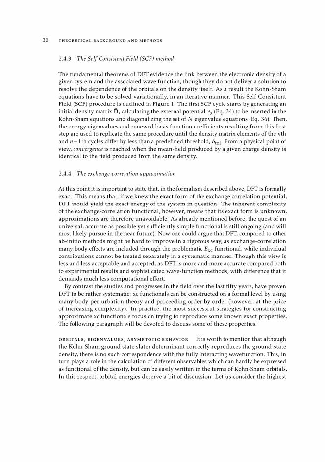
The fundamental theorems of DFT evidence the link between the electronic density of agiven system and the associated wave function, though they do not deliver a solution toresolve the dependence of the orbitals on the density itself. As a result the Kohn-Shamequations have to be solved variationally, in an iterative manner. This Self ConsistentField (SCF) procedure is outlined in Figure 1. The first SCF cycle starts by generating aninitial density matrix D, calculating the external potential vs (Eq. 34) to be inserted in theKohn-Sham equations and diagonalizing the set of N eigenvalue equations (Eq. 36). Then,the energy eigenvalues and renewed basis function coefficients resulting from this firststep are used to replicate the same procedure until the density matrix elements of the nthand n−1th cycles differ by less than a predefined threshold, δtol. From a physical point ofview, convergence is reached when the mean-field produced by a given charge density isidentical to the field produced from the same density.
2.4.4 The exchange-correlation approximation
At this point it is important to state that, in the formalism described above, DFT is formallyexact. This means that, if we knew the exact form of the exchange correlation potential,DFT would yield the exact energy of the system in question. The inherent complexityof the exchange-correlation functional, however, means that its exact form is unknown,approximations are therefore unavoidable. As already mentioned before, the quest of anuniversal, accurate as possible yet sufficiently simple functional is still ongoing (and willmost likely pursue in the near future). Now one could argue that DFT, compared to otherab-initio methods might be hard to improve in a rigorous way, as exchange-correlationmany-body effects are included through the problematic Exc functional, while individualcontributions cannot be treated separately in a systematic manner. Though this view isless and less acceptable and accepted, as DFT is more and more accurate compared bothto experimental results and sophisticated wave-function methods, with difference that itdemands much less computational effort.
By contrast the studies and progresses in the field over the last fifty years, have provenDFT to be rather systematic: xc functionals can be constructed on a formal level by usingmany-body perturbation theory and proceeding order by order (however, at the priceof increasing complexity). In practice, the most successful strategies for constructingapproximate xc functionals focus on trying to reproduce some known exact properties.The following paragraph will be devoted to discuss some of these properties.
orbitals, eigenvalues, asymptotic behavior It is worth to mention that althoughthe Kohn-Sham ground state slater determinant correctly reproduces the ground-statedensity, there is no such correspondence with the fully interacting wavefunction. This, inturn plays a role in the calculation of different observables which can hardly be expressedas functional of the density, but can be easily written in the terms of Kohn-Sham orbitals.In this respect, orbital energies deserve a bit of discussion. Let us consider the highest
2.4 enforcement of the kohn-sham approach 31
Guess initial density matrix D0
v(n)s [ρ(r)] = v(r) +
∫R3 dr’ ρ(r’)
r−r’ + ∂Exc∂ρ(r)
∣∣∣∣∣∣ρ=ρn
∀i ∈ [1,N ];
−12∇2
i ϕ(n)i (r) + v
(n)s ϕ
(n)i (r) =
∑Nj ε
(n)ij ϕ
(n)j (r)
E[ρn] = EKS[ρn]−∫R3 dr ρn(r)
∂Exc∂ρ(r)
∣∣∣∣∣∣ρ=ρn
+Exc[ρ]ρn+1(r) = 2∑N/2i ϕ
∗(n)i (r)ϕ
(n)i (r)
| E[ρn]−E[ρn+1 |≥ δtol
Self-concistency!Optimized wavefunction
at given geometry
NO
YES
Figure 1: Flowchart of the SCF procedure within the DFT approach
32 theoretical background and methods
occupied eigenvalue εN of an N -electron system. According to Koopmans’ theorem[40, 41] εN equals the negative of the ionization potential (IP ) of the system - i.e. theenergy required to remove an electron from the system and place it at infinite distance.We may therefore write,
εN (N ) = E(N )−E(N − 1) = −IP (N ), (53)
where E(N ) and E(N − 1) denote the energies of the N - and N − 1-electron systems,respectively. Hence, εN has a rigorous physical meaning. The same does not hold truefor all other energy eigenvalues εj . However, one can still relate the lowest unoccupiedeigenvalue εN+1 to the electron affinity (EA) - the energy gained as an electron - placedat infinite distance - is added to the system. Therefore,
εN+1(N + 1) = E(N + 1)−E(N ) = −EA(N ), (54)
Because the LUMO is not correctly reproduced (the reason for this will be better explainedin the following), the Kohn-Sham excitation energy (εa−εi ) differs from the exact excitationenergy of a many-body system - a and i denote a virtual and an occupied orbital. Althoughone may use the former as a first approximation, the orbital difference will get closer tothe exact value, the more accurately the unoccupied levels are described. This of coursedepends on the quality of the approximate xc functional used.
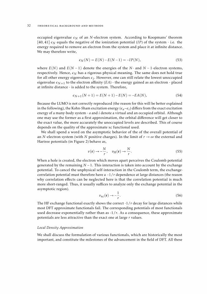
We shall spend a word on the asymptotic behavior of the of the overall potential ofan N -electron system (with N positive charges). In the limit of r→∞ the external andHartree potentials (in Figure 2) behave as,
v(r)→−Nr
, vH(r)→ Nr
. (55)
When a hole is created, the electron which moves apart perceives the Coulomb potentialgenerated by the remaining N − 1. This interaction is taken into account by the exchangepotential. To cancel the unphysical self-interaction in the Coulomb term, the exchange-correlation potential must therefore have a −1/r dependence at large distances (the reasonwhy correlation effects can be neglected here is that the correlation potential is muchmore short-ranged. Thus, it usually suffices to analyze only the exchange potential in theasymptotic region).
vxc(r)→−1r
. (56)
The HF exchange functional exactly shows the correct -1/r decay for large distances whilemost DFT approximate functionals fail. The corresponding potentials of most functionalsused decrease exponentially rather than as -1/r. As a consequence, these approximatepotentials are less attractive than the exact one at large r values.
Local Density Approximation
We shall discuss the formulation of various functionals, which are historically the mostimportant, and constitute the milestones of the advancement in the field of DFT. All these
2.4 enforcement of the kohn-sham approach 33
r
v(r
)
External potential, r →∞
N = 1
N = 2
N = 3
r
v H(r
)
Hartree potential, r →∞
N = 1
N = 2
N = 3
Figure 2: Schematic depiction of the asymptotic behavior of the external and Hartree potentials.
formulations differ by the functional dependence of Exc on the electron density. This isexpressed as the intergral of the product between the electron density and a so-calledenergy density εxc that depends explicitly on the electron density:
Exc[ρ] =
∫drρ(r)εxc[ρ(r)]. (57)
Here, the energy density is a sum of individual exchange and correlation contributions.The Local Density Approximation, [37] takes into account the energy density at each
position r, computed using the value of ρ at that same position - therefore the functionalis local.
ELDAxc [ρ(r)] =
∫drρ(r)εxc[ρ(r)]ρ=ρ. (58)
In practice, the functionals of this class that are still applied are those that derive fromthe uniform electron gas [42]. For each given point the exchange-correlation energy iscomputed as the energy of a uniform electron gas of the same local density.
Generalized Gradient Approximation and Kinetic Energy Density
As the electron density is typically rather inhomogeneous, LDA suffers of severe limita-tions. An obvious way to get over these limitations - at least partially - is by constructingexchange correlation functionals which depend not only on the local value of the densitybut also on its gradient. Usually, gradient corrected functionals are obtained by adding acorrection term to the LDA functional:
εGGAxc [ρ(r)] = εLDA
xc [ρ(r)] +∆εxc
[ |∇ρ(r)|ρ4/3(r)
], (59)
where the correction depends on the dimensionless reduced gradient( |∇ρ(r)|ρ4/3(r)
). This
class of functionals is generally referred to as the Generalized Gradient Approximation(GGA) [43].
If including the gradient of the density constitutes an improvement over LDA, a logicalstep forward - in the same vein as a Taylor expansion - is to use higher order derivatives
34 theoretical background and methods
of the density. The so-called meta-GGA (mGGA) [44] functionals are constructed usingthe second order derivative. However, instead of including the Laplacian of the density -which often leads to numerical instabilities - they are formulated using the Kohn-Shamorbital kinetic energy densities τ that one can prove to be connected to the Laplacian,
τσ (r) =occ∑i
12|∇ϕ(r)|2. (60)
Adiabatic connection and hybrid functionals
According to Kohn-Sham scheme the Exc functional is defined assuming a fully non-interacting reference system of particles. Instead one could imagine to follow up theextent of the electron-electron interaction with an extra parameter. This last is the ideawhich underlies the adiabatic connection formalism [45], which make it possible toestablish the relationship between the real and the non-interacting system [34]. Theadiabatic connection follows directly from the Hellmann–Feynman, which relates thederivative of the total energy with respect to a parameter, to the expectation value ofthe derivative of the Hamiltonian with respect to that same parameter. As a result, theexchange-correlation energy can be expressed as,
Exc[ρ] =
∫ 1
0
⟨Ψ (λ)
∣∣∣Vxc[ρ](λ)∣∣∣Ψ (λ)
⟩, (61)
where the parameter λ controls the amount of electron-electron interaction, which variesbetween 0 and 1. Using the adiabatic connection formalism, one can express the exchange-correlation potential as a function of λ. This results in a polynomial function of degreen− 1, and dependent on the parameter λ, which controls the mixing of both the exchangeand correlation from DFT, and the HF exchange. In other words, n controls the speed withwhich the correction brought to DFT is canceled when λ tends towards the unit,
Uλxc[ρ] = EDFTxc,λ [ρ] + (EHF
x −EDFTx [ρ])(1−λ)n−1. (62)
Integration of this relation (67) over the interval λ ∈ [0,1] then gives:
Exc[ρ] =
∫ 1
0dλUλxc[ρ] (63)
= EDFTxc [ρ] +
1n(EHF
x +EDFTx [ρ]) (64)
The parameter λ allows one to go smoothly from the fully non-interacting to the inter-acting system - at a fixed density value (ρ0). Thus, the exchange-correlation energy isnothing other than the average of the exchange-correlation hole, Eh,
Exc[ρ] =
∫ 1
0
⟨Ψ (λ)
∣∣∣Vee[ρ](λ) ∣∣∣Ψ (λ)⟩− J [ρ] = Eh[ρ]. (65)
2.4 enforcement of the kohn-sham approach 35
λ
Exc
EHFx
−E
0 1A
B
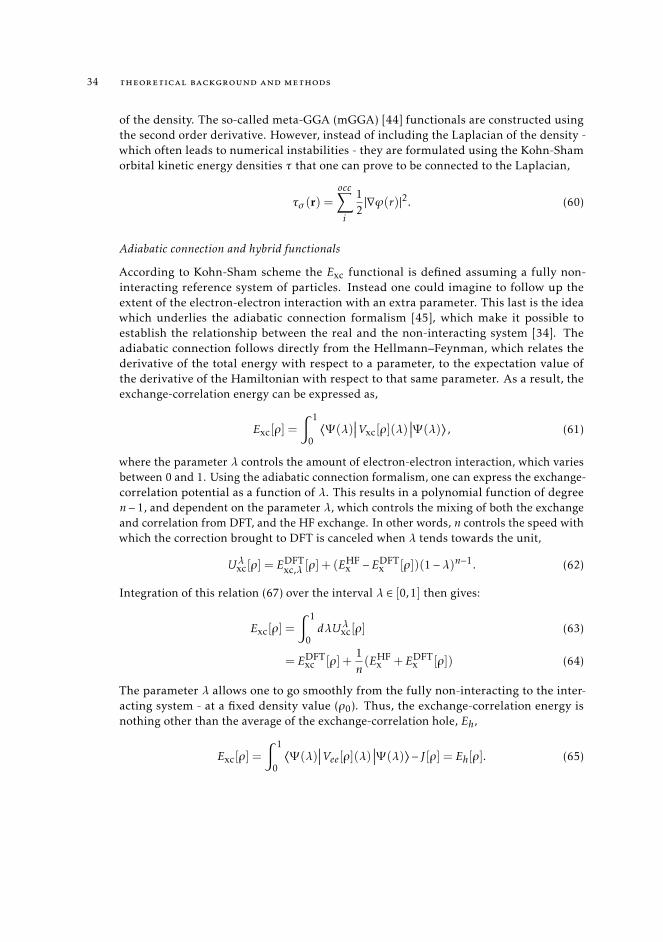
Figure 3: Pictorial representation describing the adiabatic connection method. Rectangle A representsthe fully non-interacting system, for which we only have exchange interaction. The fullexchange-correlation energy is represented by the sum of the area of rectangle A and thatunder the green curve in rectangle B
A graphical representation of this integral is particularly insightful. Figure 3 depictsthe electron-electron interaction, partitioned into two portions -the lower rectangle, A,and the fraction of upper rectangle delimited by the green line, B. The bottom rectanglerepresents the fully non-interacting system - in which the only contribution to the electron-electron interaction is the non-classical exchange term Eh (EHF
x in Hartree-Fock). Theupper rectangle, instead, depicts the contribution of the electronic interaction due tothe exchange-correlation energy. At λ = 1 the total interaction energy relative to thelower portion is thus 1 times the exact exchange (HF) energy EHF
x . The formal differencebetween Eh and EHF
x is that they are derived using Kohn-Sham orbitals and HF orbitals,respectively. The remaining interaction energy is represented by the area under the greencurve in rectangle B, i.e. some fraction x of rectangle B. As we do not know x, nor theexpectation value of the fully interacting exchange-correlation potential, we may onlyregard x as a parameter to optimize. Thus, one can approximate the fully interactingsystem (upper right corner of B) using some choice of DFT functional, weighted by anappropriate value of x. Using this strategy, the total area under the curve (A+xB) can beapproximated as:
Exc[ρ] = EHFx + x(EDFTxc [ρ]−EHF
x ) (66)
It is convention to express Exc in terms of an alternative parameter, a, defined as 1− x,yielding:
Exc = (1− a)EDFTxc [ρ] + aEHFx (67)
In practice, Eq. 67 draws the connection between the interacting and non-interactingsystems by mixing a fraction of exact exchange, derived from HF theory [38] with a
36 theoretical background and methods
standard LDA or GGA. This concept forms the basis for what are known as hybrid densityfunctionals.
One such Hybrid Functional, widely known as PBE0 [46], is constructed using a valueof a = 0.25 (i.e. 25% HF exchange):
Exc[ρ] = EPBExc [ρ] +
14(EHFx +EPBE
x [ρ]), (68)
where the xc functional used to approximate the fully-interacting system is that of Perdew,Burke and Ernzerhoff - known as PBE [43].
2.4.5 Self-interaction and derivative discontinuities
DFT is in principle an exact theory. However, the construction of approximate exchange-correlation functionals leads to basic flaws. Hence, the resulting density functionalapproximations (DFA) are affected by different sources of error, where by DFA we meanany standard approximation to the exchange-correlation energy within DFT. Among theknown errors, the self-interaction error (SIE) in DFAs appears from the fact that theresidual self-interaction in the Coulomb part and that in the exchange part do not canceleach other exactly. This error is responsible for the unphysical orbital energies of DFTand the failure to reproduce the potential energy curves of several physical processes. Aspreviously mentioned, the Kohn-Sham excitation energy differs from the exact excitationenergy of a many-body (interacting) system. If we where to express the exact excitationenergy Eex in terms of the Kohn-Sam eigenvalues, we would write,
Eex(N ) = εN+1(N + 1)− εN (N ). (69)
By contrast in the non-interacting system the excitation energy Eex,s is simply the differ-ence between the highest occupied and lowest unoccupied single-particle orbital,
Eex,s(N ) = εN+1(N )− εN (N ). (70)
Then, we may relate the two excitation energy values as,
Eex(N ) = Eex,s(N ) +∆xc. (71)
In this expression, ∆xc is the so-called derivative discontinuity, a known source of error inDFT. This term is related to the fact that Exact vxc(r) jumps discontinuously by a constantamount ∆xc - several eV - as N crosses the integer. This in turn has the consequence thatan accurate continuous potential should not vanish asymptotically but rather decay as
limr→∞vxc(r) = −1
r. (72)
This phenomenon reflects the chemical potential to exchange particles between twosystems -i.e, it ensures that heteroatomic molecules dissociate to neutral fragments. Againthe exchange part of HF models this behavior correctly, while none of the standard
2.4 enforcement of the kohn-sham approach 37
approximate functionals, which are all characterized by a continuous potential withrespect to variations in the number of electrons, is able to do this. Hybrid functionals,which incorporate a fraction of exact exchange do rectify these problem to some extent.In this respect, one could think that simply increasing the amount of HF exchange to100% would solve the problem. In practice, turns out that this is just a sham solution, asit introduces the substantial error related to the lack of correlation-effects in HF.
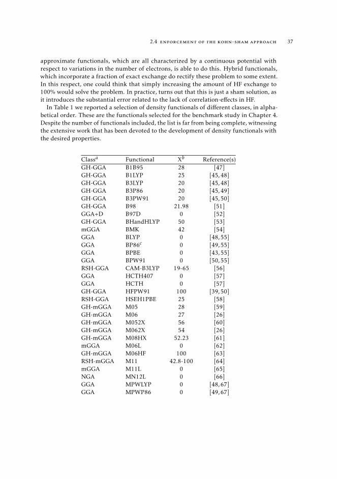
In Table 1 we reported a selection of density functionals of different classes, in alpha-betical order. These are the functionals selected for the benchmark study in Chapter 4.Despite the number of functionals included, the list is far from being complete, witnessingthe extensive work that has been devoted to the development of density functionals withthe desired properties.
Classa Functional Xb Reference(s)GH-GGA B1B95 28 [47]GH-GGA B1LYP 25 [45, 48]GH-GGA B3LYP 20 [45, 48]GH-GGA B3P86 20 [45, 49]GH-GGA B3PW91 20 [45, 50]GH-GGA B98 21.98 [51]GGA+D B97D 0 [52]GH-GGA BHandHLYP 50 [53]mGGA BMK 42 [54]GGA BLYP 0 [48, 55]GGA BP86c 0 [49, 55]GGA BPBE 0 [43, 55]GGA BPW91 0 [50, 55]RSH-GGA CAM-B3LYP 19-65 [56]GGA HCTH407 0 [57]GGA HCTH 0 [57]GH-GGA HFPW91 100 [39, 50]RSH-GGA HSEH1PBE 25 [58]GH-mGGA M05 28 [59]GH-mGGA M06 27 [26]GH-mGGA M052X 56 [60]GH-mGGA M062X 54 [26]GH-mGGA M08HX 52.23 [61]mGGA M06L 0 [62]GH-mGGA M06HF 100 [63]RSH-mGGA M11 42.8-100 [64]mGGA M11L 0 [65]NGA MN12L 0 [66]GGA MPWLYP 0 [48, 67]GGA MPWP86 0 [49, 67]
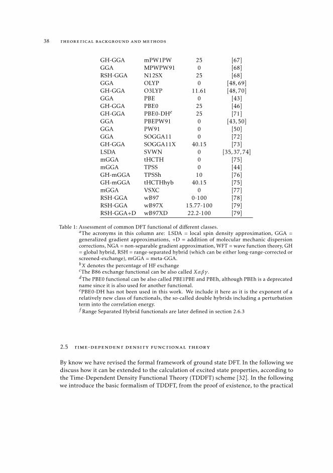
38 theoretical background and methods
GH-GGA mPW1PW 25 [67]GGA MPWPW91 0 [68]RSH-GGA N12SX 25 [68]GGA OLYP 0 [48, 69]GH-GGA O3LYP 11.61 [48, 70]GGA PBE 0 [43]GH-GGA PBE0 25 [46]GH-GGA PBE0-DHe 25 [71]GGA PBEPW91 0 [43, 50]GGA PW91 0 [50]GGA SOGGA11 0 [72]GH-GGA SOGGA11X 40.15 [73]LSDA SVWN 0 [35, 37, 74]mGGA tHCTH 0 [75]mGGA TPSS 0 [44]GH-mGGA TPSSh 10 [76]GH-mGGA tHCTHhyb 40.15 [75]mGGA VSXC 0 [77]RSH-GGA wB97 0-100 [78]RSH-GGA wB97X 15.77-100 [79]RSH-GGA+D wB97XD 22.2-100 [79]
Table 1: Assessment of common DFT functional of different classes.aThe acronyms in this column are: LSDA = local spin density approximation, GGA =generalized gradient approximations, +D = addition of molecular mechanic dispersioncorrections, NGA = non-separable gradient approximation, WFT = wave function theory, GH= global hybrid, RSH = range-separated hybrid (which can be either long-range-corrected orscreened-exchange), mGGA = meta-GGA.bX denotes the percentage of HF exchangecThe B86 exchange functional can be also called Xαβγ .dThe PBE0 functional can be also called PBE1PBE and PBEh, although PBEh is a deprecatedname since it is also used for another functional.ePBE0-DH has not been used in this work. We include it here as it is the exponent of arelatively new class of functionals, the so-called double hybrids including a perturbationterm into the correlation energy.f Range Separated Hybrid functionals are later defined in section 2.6.3
2.5 time-dependent density functional theory
By know we have revised the formal framework of ground state DFT. In the following wediscuss how it can be extended to the calculation of excited state properties, according tothe Time-Dependent Density Functional Theory (TDDFT) scheme [32]. In the followingwe introduce the basic formalism of TDDFT, from the proof of existence, to the practical
2.5 time-dependent density functional theory 39
solution of the Kohn-Sham equation. We will discuss how TDDFT can be used to calculateexcited-states of molecules, the sources of errors and limitations of this approach alongwith some approaches to overcome - at least partially - these limits.
Let us consider the usual system of N interacting (non-relativistic) electrons. Thesystem evolves in a scalar potential, which, differently from the static case is a functionboth of time and space. The total Hamiltonian varies now in time, and the associatedSchrödinger equation writes,
Hel(r, t)Ψel(r, t) = i∂∂t
Ψel(r, t), (73)
where:Hel(r, t) = Te(r) + Vee(r, t) + v(r, t). (74)
This expression retraces the time-independent one, with the difference that the timedependency is now explicitly included. Then, the first two terms are again the kineticand electron-electron repulsion terms. The final term is an external potential, which alsoevolves in time, and has the form,
v(r, t) = v0(r) +θ(t − t0)v1(r,t), (75)
where θ is the Heaviside function [80]. The time dependence is "switched-on" at times thatare greater than t0. It follows that for times t ≤ 0, the external potential is constant andtherefore reduces to what we find in the previous sections for the time-independent case.At times t0 , 0 the density will start oscillating. Such formalism provides a convenientrepresentation of the physical processes we are interested in - i.e., a molecule hit by a lightpulse. Of particular interest are those potentials that can be treated as weak perturbations.As we will show in section 2.5.3, taking the first order response to those perturbations isenough to calculate the excitation energies of a system [32].
2.5.1 Runge-Gross theorem
The time-dependent potential v(r, t) fully determines the evolution of the system, throughthe time-dependent Schrödinger equation. This means that the Schrödinger equationestablishes a formal map by which any chosen external potential V (t) produces a timedependent wave function Ψ (t), which represents the time-evolution of given initial stateΨ0. Ψ (t) can then be used to map a time-dependent density ρ(r, t),
v(t)→ Ψ (t)→ ρ(r, t) (76)
In order to legitimate the time-dependent theory this map must be inverted. Just as forthe time-independent case, we need to proof that there is a one-to-one correspondencebetween the time dependent densities and potential. By virtue of this correspondencethe density, ρ(r, t) can be used as an alternative variable to the potential to determine thetime-evolution of the system. This correspondence was first demonstrated by Runge and
40 theoretical background and methods
Gross in 1984, [81]. As a result, the many-body Hamiltonian H(t) and thus the many-bodywave function Ψ (t) are functionals of ρ(r, t).
runge-gross theorem
v(r, t) = v[ρ,Ψ0](r, t) =⇒ H(t) = H [ρ,Ψ0](t) =⇒ Ψ (t) = Ψ [ρ,Ψ0](t). (77)
2.5.2 The van Leeuven theorem
The Runge-Gross theorem does not yet offer a practical scheme - equivalent to theKohn–Sham formalism for static DFT - to calculate time-dependent densities in a simplermanner than by solving the full many-body Schrödinger equation. The theorem of vanLeeuven (1999) provides a solid foundation to the construction of such a scheme andstates the following,
van leeuven theorem Given a time-dependent density ρ(r, t), associatedwith a many-body system, with a particle-particle interactionω(|r−r′ |), an externalpotential v(r, t), and an initial state Ψ0, there exists a different many-body systemwith interaction ω′(|r− r′ |) and a distinct, unique external potential v′(r, t) whichreproduces the exact same time-dependent density - up to a time-dependentconstant c(t). The only requirement being that the initial state Ψ ′0 in this systemmust be chosen such that it reproduces the initial density and its time derivativeat t = 0.
It follows directly that under the constraint Ψ0 = Ψ ′0′ , and by imposing that the interac-tion energy of a real system can be reproduced by a fictitious one (ω(|r− r′ |) = ω′(|r− r′ |)),there exists a unique potential v(r, t) that reproduces the interacting density ρ(r, t). Thisis precisely what is stated by Runge–Gross theorem, revealing this last to be a special caseof the van Leeuwen theorem.
2.5.3 Time-dependent Kohn-Sham framework
In this section we shall introduce the formal framework of TDDFT, which can be usedto calculate excited state properties. TDDFT is able to capture the dynamical nature ofan excitation process. During a transition between the ground and a given excited state,periodic charge-density fluctuations are induced, accompanied by dynamical many-bodyeffects and mixing of Kohn-Sham eigenstates. This in turn leads to a modification ofthe original spectrum, calculated using the Kohn-Sham eigenvalues, towards the realspectrum. These dynamical many-body effects are embedded in the so-called exchange-correlation kernel (fxc), the key component of TDDFT, which plays the same role in TDDFTas the the exchange-correlation functional plays in Kohn-Sham DFT.
2.5 time-dependent density functional theory 41
Up until now, we have spoken only in terms of the time-dependent Schrödinger equation.In practice, the generation of excited states can be looked as an ultrafast process, implyingonly small deviations from the ground state. Under this perspective, attempting to findthe full solution to the time-dependent Schrödinger equation seems rather exaggerate,and unnecessary. Instead, one might attempt to calculate these deviations directly, this isprecisely what is done through the response theory [32].
Response theory, and more specifically linear response theory, is a widely used methodone can apply to study how a system responds to weak perturbations. In the context ofoptical spectroscopy techniques, the perturbation is generated by the light irradiations ofthe ground state. The linear response of the system as it interacts with the electric fieldcontains all of the information about its optical spectrum.
The Runge-Gross and van Leeuwen theorems legitimate the use of a non-interactingsystem in TDDFT, just as the Hohenberg-Kohn theorems did in ground state DFT. In thetime dependent case the density can be expressed as,
ρ(r, t) =N∑i
|Ψi(r, t)|2. (78)
These single particle orbitals satisfy the time-dependent Kohn-Sham equation,[− 1
2∇2 + vs(r, t)
]Ψi = i
∂∂t
Ψi(r, t), (79)
where the effective potential has the form,
vs(r, t) = v(r, t) +∫
R3dr′ ρ(r, t)|r− r′ | + vxc[ρ,Ψ0,Ψs0](r, t). (80)
The effective potential depends through vxc both on the initial state of the interactingsystem (Ψ0), and the initial state of the Kohn-Sham system (Ψs0). The external potentialvs(r, t) is assumed to have the form shown in equation 75. If the system of interest isinitially in the ground state, the time-dependent exchange-correlation potential vxc[ρ](r, t)can be written as a functional of the density only [32], through the so called adiabaticapproximation. In a similar vein to the approach discussed in Section 2.4.4 such approachcan be used to construct the ’time evolved’ potential from the ground state potential as,
vAxc(r, t) = vgsxc [ρ0](r)|ρ0=ρ(r,t). (81)
The adiabatic approximation guarantees that the same functionals as the one defined inSection 2.4.4 for ground state DFT can be used in TDDFT as well. These functionals havethe exact same form but are evaluated at the instantaneous time-dependent density.
42 theoretical background and methods
the linear response formalism We consider a time-dependent Kohn-Sham po-tential of the form of Eq. 75. This implies that the system is in its ground state for t ≤ t0and v1(r, t) is a small time-dependent perturbation switched on at t0. The initial many-body ground state is uniquely determined as stated by the Hohenberg-Kohn theorems ofstatic DFT, and according to the Runge-Gross theorem, there exists a unique one-to onecorrespondence between vs(r, t) and ρ(r, t). If the potential is time dependent, the densitywill be as well. Therefore we can write the time-dependent density as a functional of theexternal potential, without any dependence on the initial state.
ρ(r, t) = ρ[v](r, t) (82)
If the perturbation is weak enough, the potential can be expanded in Taylor series asfollows,
v(r, t) = v0(r) + v1(r, t) + v2(r, t) + · · · (83)
accordingly the density can be expressed as,
ρ1(r, t)− ρ0(r) = ρ1(r, t) + ρ2(r, t) + · · · (84)
where ρ0 is the ground state density, ρ1 is the first order change in density. The first orderterm will dominate over the higher order terms in the case of a weak potential so the restcan be neglected. Hence, the first order term density response can be written as,
ρ1(r, t) =∫ ∞−∞
dt′∫
Rdr′χ(r, t,r′ , t′)v1(r
′ , t′) (85)
where χ is the density-density response function [32], defined as,
χ(r,r, t − t′) = −iθ(t − t′) 〈Ψ0| [ρ(r, t − t′), ρ(r)] |Ψ0〉 (86)
The frequency dependent response function is the Fourier transform of equation 85, thatis
ρ1(r,ω) =∫
Rdr′χ(r,r′ ,ω)v1(r
′ ,ω) (87)
with
χs(r,r′ ,ω) =
∞∑n=1
〈Ψ0| ρ(r) |Ψn〉〈Ψn| ρ(r′) |Ψ0〉ω −Ωn+ iη
− 〈Ψ0| ρ(r′) |Ψn〉〈Ψn| ρ(r) |Ψ0〉ω −Ωn+ iη
(88)
where the limit η→ 0+ is known [82]. The nth excitation energy, Ωn is given by En −E0.The response function diverges when the frequency matches the excitation energy - eachof these events translate into the appearance of a peak within a spectra.
This time-dependent density ρ(r, t), corresponding to v(r, t) can also be reproduced ina non-interacting time-dependent Kohn-Sham system, with an effective potential, vs(r, t).Then, for such non-interacting system we can write,
ρ1(r,ω) =∫
Rdr′χs(r,r′ ,ω)vs1(r′ ,ω) (89)
2.5 time-dependent density functional theory 43
This is the linear response equation in TDDFT, which is the density-density responsefunction for a non-interacting Kohn-Sham particles and yields the same response as thefully interacting, many-body response equation. Similar to equation 80 the effectivepotential writes,
vs[ρ](r, t) = v(r, t) +∫
R3dr′ ρ1(r, t)|r− r′ | + vxc(r, t). (90)
The perturbation acts at each t giving rise to a retarded density response at all r, andall of these are then integrated over space. The density-density response function fornon-interacting particles is expressed as,
χs =δρ[vs](r, t)δvs(r′ , t′)
∣∣∣∣∣∣∣vs [ρ0](r)
. (91)
While the first two terms in Eq. 90 can actually be written down, the last term - thelinearized exchange-correlation potential - can be written explicitly only via a functionalTaylor expansion:
vxc =
∫ ∞−∞
dt′∫
R3dr′ δvxc[ρ](r, t)
ρ(r′ , t′)
∣∣∣∣∣∣∣ρ0(r)
ρ1(r′ , t′). (92)
This expansion reveals the so-called time dependent exchange-correlation kernel:
fxc(r, t,r′ , t′) = δvxc[ρ](r, t)ρ(r′ , t′)
∣∣∣∣∣∣∣ρ0(r)
, (93)
which is a functional of the ground state density. As previously alluded to, the kernel is thekey quantity of TDDFT in the linear response regime. Now that we have an expression forthe linearized potential vxc we can substitute it into the TDDFT linear response equation85 and get:
ρ1(r, t) =∫ ∞−∞
dt′∫
R3dr′χs(r, t,r′ , t′)×[
v1(r′ , t′) +
∫ ∞−∞
dt′′∫
R3dr′′
δ(t′ − t′′)|r′ − r′′ | + fxc(r
′ , t′ ,r′′ , t′′)ρ1(r
′′ , t′′)]
︸ ︷︷ ︸:=vs1linearized effectivee potential
. (94)
where the doubly primed variables r′′ and t′′ are used to emphasize the different doubleintegrals. This expression highlights the dependency of the linearized potential onρ1(r, t), and thus demonstrates that the overall linear density response must be solved
44 theoretical background and methods
self-consistently. The interacting and non-interacting response functions only depend onthe time difference t − t′ , therefore we can Fourier transform the Eq. 94 and obtain,
ρ1(r,ω) =∫
R3dr′χs(r,r′ ,ω)
[v1(r
′ ,ω)
+
∫R3dr′′
1
|r′ − r′′ | + fxc(r′ ,r′′ ,ω)
ρ1(r
′′ ,ω)].
(95)
The frequency dependent, non-interacting Kohn-Sham response function is given by
χs(r,r′ ,ω) =
∞∑j,k=1
(fk − fj )ϕ0j (r)ϕ
∗0k (r)ϕ∗0j (r′)ϕ0
k (r′)
ω −ωjk − iη(96)
where fk and fj are the occupation numbers on the ground state Kohn-Sham orbitalsand ωjk = εj − εk are the differences between the Kohn-Sham eigenvalues. The structureof the double summation in χs(r,r′ ,ω) is such that only those terms contribute whereone summation index refers to an occupied orbital (f = 1) and the other refers to anunoccupied orbital (f = 0), all other terms cancel out. This means that the absolutevalues of the quantities ωjk are the excitation energies of the Kohn–Sham system.Thedenominator is such that the non-interacting Kohn–Sham response function χs has polesat the excitation energies of the Kohn–Sham system. It is important to notice that thetransition energies of the non-interacting system (ωjk = εj − εk) are different comparedto Ωn - excitation energies of the real system. This apparent inconsistency, however, isresolved during the self consistent solution of the density response which cancels out thewrong poles and leaves the correct ones [32].
2.5.4 Spin-dependent formalism
For brevity, in the discussion above, we have not included the spin explicitly. However,linear response TDDFT is more commonly applied in an explicitly spin-dependent formal-ism. Moreover, several reductions of the TDDFT scheme can be better understood if thespin dependent formalism is used. Therefore, it is useful to write down the generalizationof the essential equations derived in the previous section [83]. The linear spin-densityresponse is given by
ρ1σ (r,ω) =∑σ ′
∫Rdr′χs,σσ ′ (r,r′ ,ω)vs1σ ′ (r′ ,ω). (97)
The spin-dependent linearized effective potential is,
vs1σ (r, t) = vs1σ (r,ω)∑σ ′
∫R3dr′
1|r− r′ | + fxc,σσ ′ (r,r′ ,ω)
ρ1σ ′ (r
′ ,ω).]
(98)
2.5 time-dependent density functional theory 45
The non-interacting Kohn-Sham response function is diagonal in the spin indices:
χs,σσ ′ (r,r′ ,ω) = δσσ ′
∞∑j,k=1
(fkσ − fjσ )ϕ0jσ (r)ϕ
∗0kσ (r)ϕ
∗0jσ (r
′)ϕ0kσ (r
′)ω −ωjkσ − iη
(99)
where fkσ and fjσ are the occupation numbers of the Kohn-Sham orbitals and
ωjkσ = εjσ − εkσ (100)
2.5.5 Excitation energies in TDDFT
At this point, we summarize that the exact excitation energies Ωn are given by the poles ofthe density-density response function, and the density response diverges if the system issubjected to any perturbation at such a frequency. In practice, in a system of N-electrons,excitations can be considered as a dynamic transition between two eigenstates. In thispicture the excitation energies correspond to a characteristic eigenmode of the interactingsystem [32]. An external perturbation is not even required: a system can sustain a finiteresponse at its excitation frequencies without any external stimulation, as this finiteresponse has in fact the desired character of eigenmode of the system. In order to calculatethe eigenmodes and eigenfrequencies we start from the linear-response equation withoutan external perturbation v1,
ρ1σ (r,Ω) =∑σ ′σ ′′
∫R3dr′χs,σσ ′ (r,r′ ,Ω)
∫R3dr′′fHxc,σ ′σ ′′ (r
′ ,r′′ ,Ω)ρ1σ ′′ (r′′ ,Ω)
](101)
where,
fHxc,σσ ′ (r′ ,r′′ ,Ω) =
∫R3dr′
1|r− r′ | + fxc,σσ ′ (r
′ ,r′′ ,Ω)
ρ1(r
′ ,Ω) (102)
Equation 101 is an eigenvalue equation of a frequency-dependent integral operator actingon ρ1(r,Ω), and the frequencies Ω which give the eigenvalue 1 are the excitation energieswe are looking for. This eigenvalue equation can be written in the following compactmatrix notation known as Casida equation [84], from which the eigenmodes can becalculated as, (
A B
B A
)(XY
)=Ω
( −1 00 1
)(XY
)(103)
where matrix elements of A and B are:
Aiaσ ,i′a′σ ′ (Ω) = δii′δaa′δσσ ′ωi′a′σ ′
+
∫R3dr
∫R3dr′ϕ∗0iσ (r)ϕ
0aσ (r)fHxc(r
′ ,r′′ ,Ω)ϕ0i′σ ′ (r’)ϕ∗0a′σ ′ (r’)︸ ︷︷ ︸
Kiaσ ,i′a′σ
(ω)
Biaσ ,i′a′σ ′ (Ω) = Kiaσ ,i′a′σ ′ (Ω)
(104)
46 theoretical background and methods
and
Xiaσ (Ω) = −∑σ ′
∑jk
fjσ − fkσΩ−ωjkσ ′
∫R3dr
∫R3dr′ϕ0∗
iσ (r)ϕ0aσ (r)fHxc(r
′ ,r′′ ,Ω)ϕ0i′σ ′ (r’)ϕ∗0a′σ ′ (r’)
1Ω−ωiaσ ′(105)
Yiaσ (Ω) = −Xiaσ (Ω) (106)
A and B are sometimes referred to as the orbital rotation Hessians [32]. Note that, thematrix pseudo-eigenvalue equation has infinite dimension, so in practice we only solve fora given number of excitation energies (i.e. a predefined number of eigenvalues). Generally,the accuracy of an eigenvalue associated with a given excitation energy increases withthe number of higher-energy eigenvalues computed, meaning that one should usuallyconsider a greater number of excited states than explicitly required. Moreover equation103 is only defined where fj − fk , 0, therefore only transitions from unoccupied tooccupied Kohn-Sham states (and vice-versa) will finally be considered. In general, theCasida equation returns the exact excitation energies of any many-body system. In orderto obtain exact excitation energies however, certain conditions must be met.
• One should have knowledge of the exact Kohn-Sham ground state of the system,which implies that the exact density of the density functional should be known. Ontop of this one should solve the Casida equation for all possible occupied-virtualtransitions, including the continuum states.
• This would of course require the knowledge of the exact, frequency-dependentexchange-correlation kernel, fxc, using which one should solve the infinite eigen-value problem.
• Not to mention that since the matrix elements of A and B explicitly depend onthe frequency via the exchange-correlation kernel, all this must still be done in aself-consistent manner.
Needless to say that, in practice, none of these conditions can be fulfilled exactly. Therefore,approximations must be introduced. It is also important to note that setting the couplingmatrix elements Kiaσ ,i′a′σ ′ to zero simply yields the Kohn-Sham excitation energies ωijas eigenvalues; these are single excitations. Therefore, no double or multiple excitationsare accounted for in TDDFT. On the other hand, if we were to possess an exact, frequency-dependent kernel, we would obtain poles of the many-body response function Ω withmultiple-excitation character. In the following we discuss some additional reasons whythis is never true in real life.
2.5.6 The adiabatic approximation in TDDFT
As outlined above, the key quantity in TDDFT is the frequency dependent exchange-correlation kernel, which describes the frequency dependent exchange-correlation po-tential vxc[ρ](r,ω). In analogy to ground-state DFT, application of TDDFT requires anapproximation of this potential. The simplest approximation to make here would be to
2.5 time-dependent density functional theory 47
transfer the exchange-correlation functionals used in ground-state DFT (e.g. GGA, HybridFunctionals) to the excited state, where we substitute the frequency-dependent densityfor the ground state density, according to Equation 81. In TDDFT, this is known as theadiabatic approximation [32]. The term adiabatic indicates that vAxc(r,ω) becomes exactwhere a perturbation acting on the system is sufficiently slow. In reality, this condition israrely realized, however the adiabatic approximation is used in almost all applicationsof TDDFT in chemistry. A consequence of this approximation is that in practice the xckernel is not truly frequency dependent, and only singly-excited states may be accessedwithin the adiabatic approximation.
2.5.7 Reductions of the TDDFT scheme
The Casida equation [84] is often cast into the alternative form
CZ =Ω2Z. (107)
To arrive at this expression, one assumes that the Kohn-Sham orbitals are real and that fxcis frequency-independent, so that the matrices A and B become real. Then C and Z canbe defined as,
C = (A−B)1/2(A+B)(A−B)1/2, (108)
Z = (A−B)1/2(X −Y ). (109)
Using the explicit forms of the matrix elements of A and B one finds∑i′a′σ ′
[δii′δaa′δσσ ′ω2a′ i′σ ′ ] +
√ωaiσωi′a′σ ′Kiaσ ,i′a′σ ′ ]Zi′a′σ ′ =Ω2Ziaσ . (110)
This approximate version of the Casida equation is implemented in most TDDFT codes.The eigenvalues of the Casida equation in the form of Eq. 108 are the squares of theexcitation energies; this means that for each excitation energy Ωn the Casida equationalso delivers the corresponding negative value, −Ωn. Physically, the pair (Ωn, −Ωn)corresponds to the excitations and de-excitations of the system.
2.5.8 Tamm-Dancoff approximation
The Tam-Dancoff approximation (TDA) is the exact TDDFT linear response scheme inwhich all de-excitation processes are neglected. In practice, one simply neglects theoff-diagonal matrices B in the Casida equations, keeping the matrix A unvaried. As aresult, the eigenvalue problem reduces to
AX =ΩX (111)
Further simplification of the original Casida equation can be achieved by neglecting allthe off-diagonal terms, both in the matrices A and B. Such approach follows from the the
48 theoretical background and methods
evidence that the coupling matrix elements Kiaσ ,i′a′σ decay relatively rapidly away fromthe diagonal, because the overlap of increasingly different orbitals becomes smaller bycancellation of oscillations. This scheme is known as small-matrix approximation (SMA).
Ω2± = ω2iaσ + 2ωiaσ [Kiaσ ,iaσ (Ω)±Kiaσ ,iaσ (Ω)] (112)
The SMA can be simplified further by making the TDA, i.e., by including only the positiveexcitation energy, which leads to
Ω± = ωiaσ + [Kiaσ ,iaσ (Ω)±Kiaσ ,iaσ (Ω)] (113)
Neglecting the frequency-dependence of the xc Kernel yields the single-pole approxima-tion (SPA),
Ω± = ωiaσ + [Kiaσ ,iaσ (ωiaσ )±Kiaσ ,iaσ (ωiaσ )] (114)
Under the assumption that the Kohn-Sham ground state is not spin-polarized, so thatωia↑ = ωia↓ = ωia the SPA has the following two solutions
Ω+ = ωia+ 2∫
Rdr
∫Rdr′φ0∗
i (r)φ0a (r)
[ 1r− r′ + fxc(r,r′ ,ωia)
]φ0∗i (r′)φ0
a (r′) (115)
Ω− = ωia+ 2∫
Rdr
∫Rdr′φ0∗
i (r)φ0a (r)gxc(r,r′ ,ωia)φ0∗
i (r′)φ0a (r′) (116)
where
fxc(r,r′ ,ω) = 12[fxc ↑↑ (r,r′ ,ω) + fxc ↑↓ (r,r′ ,ω)] (117)
gxc(r,r′ ,ω) = 12[fxc ↑↑ (r,r′ ,ω)− fxc ↑↓ (r,r′ ,ω)] (118)
where fxc ↑↑ and fxc ↑↓ are the spin-independent xc kernels defined in 2.5.5. In general,the TDA, and further simplified schemes yield excitation energies of comparable accuracy,as compared with TDDFT, with better convergence and lower memory requirements.However, the sum rules are not fulfilled. As a result, quantities such as the oscillatorstrength are poorly reproduced [85].
2.6 time-dependent dft and charge-transfer states
One of the drawbacks of TDDFT when using local density functionals such as LDAor GGA is its inability to routinely and accurately describe excitations of long-rangespacial extent, therefore, a note of caution is appropriate when spatially extended Rydbergexcitations and charge transfer (CT) states are concerned. Such excitations can occur in awide range of systems, such as in molecular aggregates or intramolecularly, between twodifferent functional groups. In general, this class of excitations occurs as a one electrondisplacement between two molecular subunits, that are identified as a donor (D) and anacceptor (A). In this section we elucidate why TDDFT fails when it comes to describingCT excitations and what can be done about it.
2.6 time-dependent dft and charge-transfer states 49
2.6.1 Charge transfer states in the limit of a large separation
It is instructive to start out our discussion considering a limiting case, where a donor andan acceptor are well separated, placed at distance R one from the other. The equationruling charge transfer processes can be expressed as,
IPD = D − e− (119)
EAA = A+ e− IP −EA= D+ −A− (120)
The minimum energy required to remove an electron from a molecule is its ionizationpotential. On the other hand, the energy associated with the acquisition of an electronis known as electron affinity. The subscripts D (and A) denote that an electron has beenremoved from (added to) the donor (acceptor) fragment, respectively. Once the electrondisplacement has occurred D and A resent an attractive electrostatic interaction −1/Rgenerated by the exciton pair ( R being the charge-separation coordinate). Hence, thelowest energy boundary for a CT state, ΩCT - as derived originally by Mulliken [86] -follows from elementary arguments, as
ΩCT = IPD −EAA − 1R
(121)
It is instructive to compare this value with what we would obtain from TDDFT, in thelimit of a single excitation transferring one electron from the HOMO to the LUMO. Ifthe poles of the response function 100 are sufficiently spaced (i.e., HOMO and LUMOare well separated in energy from the neighboring orbitals) one can express the energy ofa CT state using the SPA - the simplest form of the TDDFT in which de-excitations arediscarded and spin-independent kernels are considered - as introduced in Section 2.5.8,
ΩSPACT = εaL − εdH + 2
∫R3dr
∫R3dr′ϕaL(r)ϕ
dH (r)fHxc(r,r′ ,ω)ϕaL(r)ϕ
dH (r) (122)
Here, the orbitals in question are the highest occupied ϕd(r) and lowest unoccupiedϕa(r) orbitals of the donor and acceptor moieties, respectively. Since ϕd(r) and ϕa(r)havean exponentially vanishing overlap, at large distances the final term tends to zero. As aresult, the excitation energy computed at TDDFT level collapses to the difference in theKohn-Sham orbital eigenvalues:
ΩSPACT = εaL − εdH . (123)
This result is insufficient in two different aspects. The first is the missing −1/R term, thesecond is the absence of the derivative discontinuity. From Section 2.4.5 we know that inthe limit of the exact exchange-correlation functional:
IPd = −εDFTd , EAa = −εDFT
a , (124)
50 theoretical background and methods
however, we do not possess the exact exchange-correlation functional. Within standardapproximations (i.e. GGA), DFT tends to provide excitation energies which are sig-nificantly underestimated - as the LUMO does not account for the missing derivativediscontinuity, letting local and semilocal xc functionals decay faster than 1/R. This, inturn, explains why TDDFT can often drastically fail when computing charge-transferphenomena. Hybrid xc functionals, which contain a fraction of the exact HF exchange givesome improvement over standard TDDFT approximations since they lead to larger bandgaps as compared to "pure" DFT, thus yielding xc kernels for which the matrix element inthe SPA does no vanish.
2.6.2 Improved description of charge-transfer states
Next, let us consider the same model, only this time we apply a time-dependent Hartree-Fock (TDHF) approach [20]2. Then,
ΩTDHFCT = εHF
a − εHFd −
∫R3dr
∫R3dr′ ϕa(r)ϕd(r)φa(r
′)φd(r′)|r− r′ | , (125)
which becomes, in the limit of large separation:
ωTDHFCT = εHF
a − εHFd −
1R
. (126)
This demonstrates that the exact-exchange integral is responsible for the 1/R behavior.Additionally, from Koopmans theorem [40], we know that the difference in orbital eigen-values computed with Hartree-Fock can be approximated to be equal to the differencebetween the ionization potential of the donor and the electron affinity of the acceptor.As a result, charge-transfer excitation energies computed from TDHF should be at leastqualitatively correct.
This ultimately proofs that the inclusion of exact exchange into the exchange-correlationfunctional (i.e. Hybrid functionals), results in an improved description of charge-transferexcitations. As previously alluded to, using the adiabatic approximation one can estimatethe correct amount of Hartree-Fock exchange to include in the xc kernel - bearing anoptimal balance of DFT- and HF-exchange - so to preserve the short-range qualities of agiven functional as well as to include the long range correction. This apparent trade-offproblem has been tackled by a class of functionals known as range-separated hybrids,which are discussed in the next section.
2 The basic idea of TDHF is that the many-body wave function is assumed to have the form of a Slater determinant
2.7 solvation models 51
2.6.3 Range-separated hybrid functionals
A particular class of hybrid functionals are the so called range-separated hybrids (RSH).These are constructed based on a partition of the Coulomb interaction into a long-range(LR) and a short range part (SR),
1|r− r′ | =
f (µ|r− r′ |)|r− r′ | +
1− f |r− r′ ||r− r′ | , (127)
where f is typically a function such as our functional has the properties f (mx)→ 0 = 1and f (mx)→∞= 0. The parameter µ is determined either empirically or using physicalarguments. The resulting general formula for a range-separated hybrid (RSH) is then:
ERSHxc = ESR−DFAx +ELR−HFx +EDFAc (128)
where DFA stands for ‘density functional approximation’, meaning any standard approxi-mation to the exchange-correlation energy within DFT. Since the separation function forcesthe exact-exchange contribution to Exc to be 100% at large distances, range-separatedhybrids have the correct asymptotic behavior (−1/R) while at short distances they makeuse of the full density functional approximation. In practice, RSH recover the correctasymptotic behavior of external potentials at long distances, allowing for an improveddescription of molecular properties such as polarizabilities of long-chain molecules andof charge-transfer excitations.
At several points throughout this thesis, we have employed this type of functionals forthe study of charge-transfer processes in molecular systems. In Chapter 4 we analyzethe impact that the use of different classes of functionals has on the quality of computedelectronic densities.
2.7 solvation models
Whether analyzing the absorption properties or excited state lifetime of a molecularsystem, the majority of photophysical measurements take place in solution. Accuratemodeling of the solvation environment, therefore, is crucial to reproduce experimentalvalues correctly. Modeling of solvation effects in simulations can be done implicitly orexplicitly. In brief, explicit models, include the solvent molecules, that are accountedfor either classically or quantum mechanically. Implicit models treat the solvent as acontinuum dielectric with the solute in a void cavity.The latter is by far the most commonlyemployed for modeling solute-solvent interactions and it is this method that we haveemployed throughout this work.
2.7.1 The polarizable continuum model
The polarizable continuum model (PCM) [87] represents the most frequently used implicitmethod. Two formalisms are available to compute transition energies within the PCM

52 theoretical background and methods
framework: State-Specific (SS) and Linear-Response (LR) [88, 89]. We will not go intothe details of these two approaches. It suffices to know that the former considers thesolute-solvent interaction explicitly using the difference between the ground-state andexcited state expectation values. As a consequence, it provides a more complete accountof the solute-solvent polarization in the excited states as compared to the LR formalism,which describes the corresponding energy as the direct product of transition density.The latter, however, is computationally very efficient (i.e. comparable to a gas phasecalculations) and transition properties are well defined. Hence, throughout this work wehave used this formalism to account for solvation effects into TDDFT calculations.
3METHODS FOR THE DESCR IPT ION OF ELECTRONIC
EXC ITAT IONS : AN OVERV IEW
3.1 context
In Section 1 we have introduced the general framework of photochemical processes. Inthis chapter, we will try to give an overview of the existing tools that have been developedto analyze these processes from a theoretical standpoint. In particular, these methods areaimed at quantifying the redistribution of charge density involved in the excitation, andafford a concise description of the electronic transition.
As previously alluded to in Chapter 2, any excited state calculation requires the prelimi-nary definition of a ground state reference form which the excited state can be constructed.If this ground-state reference is a Hartree-Fock (single-reference) type Slater determinant,the corresponding excited state methods that we will rely on are the configuration inter-action singles (CIS) [20] and time-dependent Hartree-Fock (TDHF) [20]. Alternatively,one may start from a Kohn-Sham type single-reference Slater determinant. In that case,the associated excited state methods we will use are the Tamm-Dancoff approximation(TDA) [90] and time-dependent density functional theory (TDDFT) [32].
All these methods construct the excited-state wave function as a linear combination ofSlater determinants, in which a virtual determinant replaces an occupied one. Through-out this work, we will mainly focus on single-reference derived excited states. However,it is important to mention that one can adapt this simple molecular orbital picture ofelectronic transitions to the general correlated wave function - as we will briefly recallin Chapter 5. The outcome of these methods can be processed to analyze any selectedelectronic transition that may be of interest for a given molecular system. In particular,the main quantity we will look at are the density distributions that are generated uponthe transition [91].
A common strategy, when it comes to analyzing excited states, consists of visualizingthe excited state filled/vacant orbitals in the ground state (canonical) basis. However,in some cases, this approach may be intractable and of difficult interpretation due to themultiple Slater determinants describing the excited state involved in the transition [31].Besides, within this framework, the orbitals depend on the ground state of reference,which may not be necessarily the best choice for the description of excited states. Awell-known methodology to avoid the ground state dependence is to introduce reduceddensity matrices, which allow for appropriate orbital transformations and result in a moreconvenient and ground state-independent representation of the excited-state picture. Aswe will discuss later in this chapter, well-known examples of the latter strategy are theuse of natural transition orbitals (NTOs), attachment/detachment densities [91, 92].
53
54 methods for the description of electronic excitations: an overview
Indeed, excited state studies based on distinct manipulation of density matrices arewidely reported in the literature. Since we are mainly concerned with one-electrontransitions, the density objects that are more suited for our purposes are reduced densitymatrices. Two major approaches exist, which differ by the definition of the densitymatrix used for the analysis of the excited state, namely the one-particle transitiondensity matrix (1TDM) and the one-particle difference density matrix (1DDM) [93].Not only these particular density matrices afford an elegant and condensed description ofelectronic transitions but, from these, one may derive a variety of useful descriptors forthe characterization of the excited state phenomena [1, 91, 94, 95].
The purpose of this Chapter is to give an overview of the methodologies which havebeen devised in the past decades to investigate the locality of excited states, highlightingthe qualities and novelty of each.
3.2 introduction
Among the first detailed analysis of excited states are the contributions of Luzanov[93, 96–102], who first introduced "explicit concepts and definite criteria" involvingestimation of excited state localization and charge transfer for interpreting electronictransitions. In particular, he first suggested discarding orbital analysis in favor of somenon-invariant entities derived from the transition density matrices [96]. The essentialquantities of this analysis, which he summarized later under the name of excited statestructural analysis (ESSA) [102], are the excitation localization indexes for the quantitativeevaluation of the total charge transfer between fragments. This charge-transfer metric isbased on the projection of the exciton wave function into the atomic spin-orbital base andmeasures the probability of an electron to transfer from a molecular fragment to another. Aposition of relevance in our overview of density based indexes is due to the charge-transfermetric (DCT) [1], which constitutes the theoretical foundation for the excited state analysiscarried out in this work. The DCT metric resides on the partition of the 1DDM and on thecorresponding definition of positive and negative charge distributions associated with theelectronic transition. Rooted on a similar apportionment of the 1DDM, Etienne [103–106]has derived several additional and insightful descriptors dedicated to the study of excitedstates topology based on centroids of charge obtained from the Attachment/Detachmentdensity matrices (originally introduced for excited states analysis by Head-Gordon [91]).Although this approach also consists of a vectorial analysis of the difference densitydistribution induced by the transition, there are some substantial differences to the DCTmetric, which we will illustrate in greater detail later in the discussion. Additionally, thesame author has substantially contributed to forming a consistent and general formalismfor the topological analysis of electronic transitions from single-reference excited statescalculations, bridging the 1DDM and the 1TDM approach [94].
The work of Plasser and Drew also deserves to be mentioned. Plasser [107–110]provides a general theory and comprehensive formalism for the correct evaluation ofexciton properties both at a molecular level and in extended systems. This is donethrough the definition of an exciton wave-function out of a many-body wave function
3.2 introduction 55
obtained through quantum-chemical excited state calculations. This theory of excitonanalysis relies on the assumption that the 1TDM can be interpreted as a two-bodyexciton wave function describing the motion of a correlated hole-electron entity. In thesame vein to what mentioned above for the 1DDM, the exciton wave function can alsobe analyzed with the aid of a series of descriptors. While the original work proposedthe analysis of this exciton wave function through a population analysis [95], later thismodel has been generalized [107,110–112]. The exciton analysis is carried out through thecomputation of the expectation value of any operator acting in the same orbital basis of the1TDM. This strategy is then proven to be independent of atom-centered basis functionsand not to require partitioning of the wave function into atom- or fragment-centeredcontributions [112].
Several other alternative descriptors exist, some of which proposed as a modification offormerly existing indexes, other being brand new definitions, aimed at further exploringthe metric of excited electronic states in the framework of density functional theory. Wecite here the ∆r approach by Guido and Adamo [113], which relies on the calculation ofthe charge centroids of natural transition orbital pairs (relevant for a given transition).This index renders the concept of average hole-electron distance upon excitation. Theauthors also address differences and similarities towards another well-known index (Λ)by Tozer and Helgaker, which measures the spatial overlap in a given excitation. AlthoughΛ may also provide an estimate of the spatial extent of an electronic transition, it is morea diagnostic tool for TDDFT methodological failures, and it was devised to establish thereliability of a general electronic transition. We will elaborate more on density indexes fordiagnostics in Chapter 6.
Another strategy consists to quantitatively characterize the charge displacement oc-curring upon excitation by integrating the electronic density along a chosen axis (whichcoincides with the electron-transfer coordinate) [114]. Altogether, these studies havecontributed to the evolution of the models employed for the study of excited states. Belowwe provide a more detailed description of some of the descriptors mentioned above. Thissummary aims at giving a comprehensive view of the methodologies that are available forexamining electronic excitations and at providing a context for the work presented lateron.
notation reminder Throughout the chapter we denote orbital indexes with threetype of subscripts,
• Atomic orbitals (AO) are denoted the letter φ with Greek subscripts: µ,ν,λ,σ
• Molecular orbitals are indicated by ϕ with corresponding indexes following theusual convention: i, j,k, l, ... for occupied; a,b,c,d, ... for virtual; p,q,r,s, ... for genericorbitals. Density matrices expressed in a canonical orbital basis are indicated by theγγγ . Density matrices expressed within the MO basis are marked with a tilde: D0. Weuse boldface characters to denote matrices and vectors and plain style to refer totheir elements.
56 methods for the description of electronic excitations: an overview
3.3 density matrices
3.3.1 One-particle transition density matrices
State density matrices and difference density matrices give rise to the most widely usedconcepts in quantum chemistry. Before discussing in more details the main methodologiesfor the analysis of excited states, we first recall some useful concepts related to transitiondensity matrices, reduced density matrices and their properties [105].
We consider again an N -electron system , described by a Slater Determinant,Ψ , whichis composed of L spin-orbitals ϕ, N of which are occupied and the remaining L−N arevirtual, constructed by a LCAO expansion of K basis function φ. Unless the basis hassome linear dependencies, L and K are the same numbers. The ground state is given asthe lower energy (0) eigenfunction,
HΨ 0(x1,x2, ...,xN ) = E0Ψ 0(x1,x2, ...,xN ), (129)
where x is a four-dimensional vector containing spatial ri and spin σ coordinates of thenth electron (with n= 1, ...,N ), xn =
∑σ=α,β rnσn. One can formally construct and excited
state asHΨ X (x1,x2, ...,xN ) = EXΨ X (x1,x2, ...,xN ). (130)
The two many-particle wave functions Ψ 0 and Ψ X may differ by any orbital substitution.Since we now compare ground state and excited state wave functions in terms of orbitalsit is instructive to express the latter in a spin-orbital basis: where the summation runsover L spin-orbitals.
Ψ X =
(∑pq
cXpqp†q+
∑pqrs
cXpqrs r†p†qs+ ...
)Ψ 0. (131)
Equivalently we could also express the same wave function in an atomic-orbital basis,
Ψ X =
(∑µν
cXµν a†µaν +
∑µνµ′ν′
cXµνµ′ν′ a†µ′ a†µaν′ aν + ...
)Ψ 0. (132)
where the summation runs over the K basis functions. Here Ψ0 is the ground state fromwhich the excited state is generated by applying a series of annihilation and creationoperators, which successively generate hole and particles in the reference wave function.Depending on the number of these operations the resulting state is singly, doubly excited,etc. Visualizing such excited wave function is not trivial. Indeed one can notice fromexpression 132 that the wave function, projected in an atomic orbital basis, depends on thechosen basis via the orbital coefficients cXµν ,cXµνµ′ν′ . Thus, the choice of basis determinesthe quality of the excited state representation and the coefficients can not be directly usedfor the analysis of excited states. However, a related concept exists, more suitable for thispurpose, that is the reduced transition density matrix.
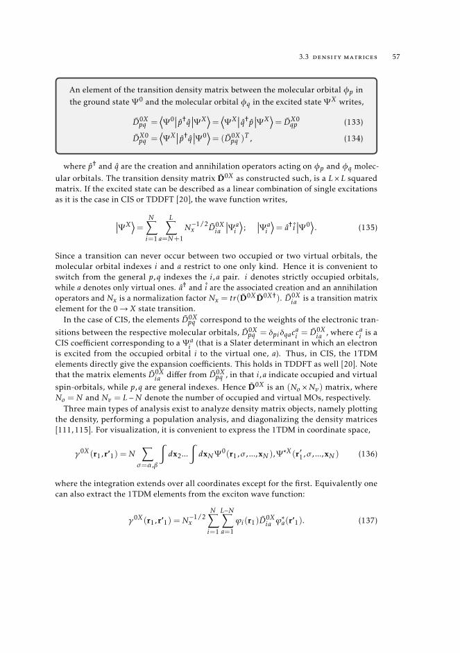
3.3 density matrices 57
An element of the transition density matrix between the molecular orbital φp inthe ground state Ψ 0 and the molecular orbital φq in the excited state Ψ X writes,
D0Xpq =
⟨Ψ 0
∣∣∣ p†q ∣∣∣Ψ X⟩=
⟨Ψ X
∣∣∣ q†p ∣∣∣Ψ X⟩= DX0
qp (133)
DX0pq =
⟨Ψ X
∣∣∣ p†q ∣∣∣Ψ 0⟩= (D0X
pq )T , (134)
where p† and q are the creation and annihilation operators acting on φp and φq molec-ular orbitals. The transition density matrix D0X as constructed such, is a L×L squaredmatrix. If the excited state can be described as a linear combination of single excitationsas it is the case in CIS or TDDFT [20], the wave function writes,
∣∣∣Ψ X⟩=
N∑i=1
L∑a=N+1
N−1/2x D0X
ia
∣∣∣Ψ ai
⟩;
∣∣∣Ψ ai
⟩= a† i
∣∣∣Ψ 0⟩
. (135)
Since a transition can never occur between two occupied or two virtual orbitals, themolecular orbital indexes i and a restrict to one only kind. Hence it is convenient toswitch from the general p,q indexes the i,a pair. i denotes strictly occupied orbitals,while a denotes only virtual ones. a† and i are the associated creation and an annihilationoperators and Nx is a normalization factor Nx = tr(D0XD0X†). D0X
ia is a transition matrixelement for the 0→ X state transition.
In the case of CIS, the elements D0Xpq correspond to the weights of the electronic tran-
sitions between the respective molecular orbitals, D0Xpq = δpiδqac
ai = D0X
ia , where cai is aCIS coefficient corresponding to a Ψ a
i (that is a Slater determinant in which an electronis excited from the occupied orbital i to the virtual one, a). Thus, in CIS, the 1TDMelements directly give the expansion coefficients. This holds in TDDFT as well [20]. Notethat the matrix elements D0X
ia differ from D0Xpq , in that i,a indicate occupied and virtual
spin-orbitals, while p,q are general indexes. Hence D0X is an (No ×Nv) matrix, whereNo = N and Nv = L−N denote the number of occupied and virtual MOs, respectively.
Three main types of analysis exist to analyze density matrix objects, namely plottingthe density, performing a population analysis, and diagonalizing the density matrices[111, 115]. For visualization, it is convenient to express the 1TDM in coordinate space,
γ0X (r1,r’1) = N∑σ=α,β
∫dx2...
∫dxNΨ 0(r1,σ , ...,xN ),Ψ ∗X (r′1,σ , ...,xN ) (136)
where the integration extends over all coordinates except for the first. Equivalently onecan also extract the 1TDM elements from the exciton wave function:
γ0X (r1,r’1) = N−1/2x
N∑i=1
L−N∑a=1
ϕi(r1)D0Xia ϕ
∗a(r’1). (137)
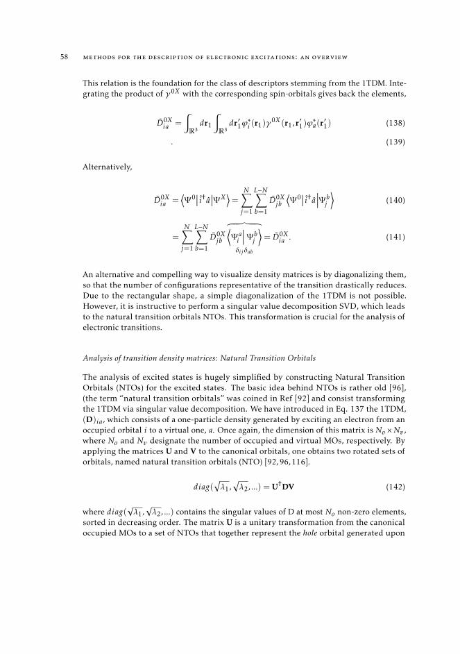
58 methods for the description of electronic excitations: an overview
This relation is the foundation for the class of descriptors stemming from the 1TDM. Inte-grating the product of γ0X with the corresponding spin-orbitals gives back the elements,
D0Xia =
∫R3dr1
∫R3dr′1ϕ
∗i (r1)γ
0X (r1,r′1)ϕ∗a(r′1) (138)
. (139)
Alternatively,
D0Xia =
⟨Ψ 0
∣∣∣ i†a ∣∣∣Ψ X⟩=
N∑j=1
L−N∑b=1
D0Xjb
⟨Ψ 0
∣∣∣ i†a ∣∣∣∣Ψ bj
⟩(140)
=N∑j=1
L−N∑b=1
D0Xjb
︷ ︸︸ ︷⟨Ψ ai
∣∣∣∣ Ψ bj
⟩δijδab
= D0Xia . (141)
An alternative and compelling way to visualize density matrices is by diagonalizing them,so that the number of configurations representative of the transition drastically reduces.Due to the rectangular shape, a simple diagonalization of the 1TDM is not possible.However, it is instructive to perform a singular value decomposition SVD, which leadsto the natural transition orbitals NTOs. This transformation is crucial for the analysis ofelectronic transitions.
Analysis of transition density matrices: Natural Transition Orbitals
The analysis of excited states is hugely simplified by constructing Natural TransitionOrbitals (NTOs) for the excited states. The basic idea behind NTOs is rather old [96],(the term “natural transition orbitals” was coined in Ref [92] and consist transformingthe 1TDM via singular value decomposition. We have introduced in Eq. 137 the 1TDM,(D)ia, which consists of a one-particle density generated by exciting an electron from anoccupied orbital i to a virtual one, a. Once again, the dimension of this matrix is No ×Nv ,where No and Nv designate the number of occupied and virtual MOs, respectively. Byapplying the matrices U and V to the canonical orbitals, one obtains two rotated sets oforbitals, named natural transition orbitals (NTO) [92, 96, 116].
diag(√λ1,
√λ2, ...) = U†DV (142)
where diag(√λ1,√λ2, ...) contains the singular values of D at most No non-zero elements,
sorted in decreasing order. The matrix U is a unitary transformation from the canonicaloccupied MOs to a set of NTOs that together represent the hole orbital generated upon
3.3 density matrices 59
transition, while V rotates the canonical virtual MOs into a new set of NTOs representingthe excited electron, conventionally named as particle,
ϕhi (rh) =No∑j=1
Ujiϕj (r), (143)
ϕpi (rp) =
Nv∑j ′=1
Vj ′ iϕ′j (r),with i = (1, ...,N ). (144)
U is the matrix diagonalizing the hole No ×No transition density matrix, expressed asTT† while V diagonalizes the particle Nv ×Nv transition density matrix T†T. U and Vmatrices are determined according to the following eigenvalue equations,
TT†ui = λoi ui , i = 1, ...,No (145)
TT†vi = λvi vi , i = 1, ...,Nv , (146)
U =
No∑i=1
ui ; V =
Nv∑i=1
vi . (147)
The new orbitals have some useful properties:
(a) Hole and particle NTOs come in pairs and their relative importance in describingthe excitation is determined by the diagonal elements of diag(
√λ1,√λ2, ...),
(b) diag(√λ1,√λ2, ...) are the excitation amplitudes in the NTO basis
(c) 1 ≥ λoi ≡ λvi ≥ 0; i = 1, ...,No
(d)∑Noi=1 = 1, in absence of de-excitation operator, as in CIS, TDA [20, 90]. We may
equivalently express the eigenvalues λi in a square-diagonal matrix, and write:
No∑i=1
λii ≡No∑j=1
(TT†)jj (148)
While in CIS the diagonal entries add up to 1, in TDDFT and RPA the sum of the λielements deviates from the unit to the extent that the de-excitation operators aresignificant. The de-excitation terms are in most cases rather small, as witnessed bythe proven ability of TDA to reproduce TDDFT values [20, 90].
(e) the eigenvectors vNo+1, ...,vNv will have zero eigenvalues.
Trough the SV decomposition, any excited state may be represented using at most Noexcitation amplitudes and corresponding hole/particle NTO pairs, rather than NoNv , asit is the case for the canonical orbitals. Thus, with each hole in the occupied space, onecan associate a single corresponding particle in the virtual space.
60 methods for the description of electronic excitations: an overview
3.3.2 One-particle reduced density matrices
Similarly to 1TDM, one can also define state density matrices or one-particle reduceddensity matrices (1RDM), which are expressions of type,
For r1 = r′1 the state density matrix reduces to the electron density.
γ0(r1r1) ≡ ρ0(r1) =L∑p=1
L∑q=1
ϕp(r1)D0pqϕ∗q(r1) (149)
⇒∫dr1 ρ
0(r1) = N . (150)
Just as for the 1TDM, integrating the product of γ0 with the corresponding spin-orbitalsgives back the elements,
D0pq =
∫R3dr1
∫R3dr′1ϕ
∗p(r1)γγγ
0(r1,r′1)ϕ∗q(r′1). (151)
One can also represent density matrices in the atomic orbital basis. For this purpose, it isuseful to introduce the density operator,
γ =N∑p=1
N∑q=1
∣∣∣ϕp(r1)⟩Dpq
⟨ϕq(r
′1)
∣∣∣ , (152)
where the Dpq are the elements of the 1RDM, expressed in MO basis. By expanding thespin-orbitals as linear a combination of atomic orbitals we get,
γ =N∑p=1
N∑q=1
K∑µ=1
K∑ν=1
∣∣∣φµ(r1)⟩CµpDpqC
∗νq︸ ︷︷ ︸
Dµν
⟨φν(r
′1)
∣∣∣ . (153)
(C)µp and (C)νq are the K ×L matrices containing the LCAO expansion coefficients. Notethat the absence of the tilde indicates that the Dµν elements are expressed in the atomicorbital basis. From the basis set expansion, we get,
N∑p=1
N∑q=1
Cµpδpν(C†)νq =
N∑p=1
Cµp(C†)pν ⇒ γ =
K∑µ=1
K∑ν=1
∣∣∣φµ(r1)⟩Dµν
⟨φν(r
′1)
∣∣∣ . (154)
The matrix elements corresponding to the density operator γ , in an atomic orbital basis,write,
Dµν =K∑ζ=1
K∑λ=1
⟨φµ(r1)
∣∣∣ φζ(r1)⟩Dζλ
⟨φλ(r
′1)
∣∣∣ φν(r′1)⟩= K∑ζ=1
K∑λ=1
SµζDζλSλν . (155)
3.3 density matrices 61
where D(K ×K) is the density matrix, and S(K ×K) is the overlap matrix expressed inatomic orbitals. Finally, we find back,
γ0(r1,r′1) =K∑µ=1
K∑ν=1
Dµνφµ(r1)φν(r′1). (156)
The total electronic density is nothing but the diagonal part of the state density matrix.Setting x = x’ and integrating the density over all space returns the number of electrons,equivalently one can compute the trace of DS.
N =K∑µ=1
K∑ν=1
∫dx1 φµ(r1)Dµνφν(r1) (157)
= T r(DS). (158)
3.3.3 Difference density matrices
In the previous section, we have introduced transition density matrices and state densitymatrices, discussing their importance in the analysis of excited states. We now introducethe one-particle difference density matrix (1DDM) [105].
Defined as the difference between the densities of two states involved in a tran-sition, the 1DDM also can be manipulated to obtain ah-hoc descriptors, for theanalysis of excited states.
γ0X∆ (r1,r′1) = γX (r1,r′1)−γ0(r1,r′1). (159)
This density matrix can be projected into the Euclidean space in order to directlyvisualize the negative and positive contributions, for instance after the light-inducedcharge displacement.
ρ∆(r1) =L∑p=1
L∑q=1
ϕp(r1)D∆pqϕ∗q(r′1) = ρX (r1)− ρ0(r1). (160)
As for the case of transition densities, plotting the difference density is not very instructive,as γγγ∆ is a complicated function [105].
ρ0X∆ (r1) = γ0X
∆ (r1,r1) = γX (r1,r1)−γ0(r1,r1) = ρX (r1)− ρ0(r1). (161)
Besides, just as for the transition density, the integral of the difference density overall space is zero, since no fraction of charge adds up or vanishes during the electronictransition: ∫
dr1 ρ0X∆ (r1) = 0. (162)
62 methods for the description of electronic excitations: an overview
Again, a more instructive way to analyze the difference density matrix is to partition it.Several methods exist, based on the diagonalization of the 1DDM or the construction of apositive and negative severance of this initial distribution.
3.4 density descriptors derived from the 1ddm
In this section we provide an overview of the most important descriptors that appeared inthe literature in the last years. For a recent review on the subject we refer to [115]. Amongthese an important class is the one of the descriptors that are derived from the 1DDM.These objects are aimed at obtaining meaningful quantities for the analysis of 1DDMs andallow an insightful interpretation of excited states.
3.4.1 The DCT index, a charge-transfer distance derived in real space
Some years ago, a simple model was proposed to define a measure of the length of a CTexcitation solely from the total electronic density in a real-space representation [1,117],computed for the ground and excited states. This idea is condensed in a descriptor, thatwe will refer to as DCT. In the following, we present the mathematical derivation ofthe DCT. In light of its simple formulation, it becomes clear that this method appliesto any quantum chemical method supplying densities for the ground and excited statesand provides in principle an effortless way to qualitatively compare the outcomes ofpost-Hartree-Fock (HF) and DFT-based approaches [3].
Let ρ0(r) and ρX (r) be the electronic densities associated to the ground and excitedstate X, respectively. The density variation associated to the electronic transition ρ∆(r) isgiven by Eq. 159. From the density difference, one can define two functions ρ+(r) andρ−(r), which collect the points in space where an increment or a depletion of charge hasoccurred due to the transition:
ρ+(r) =
ρ∆(r) if ρ∆(r) > 0
0 if ρ∆(r) < 0(163)
ρ−(r) =ρ∆(r) if ρ∆(r) < 0
0 , if ρ∆(r) < 0.(164)
It is instructive to calculate the barycenters of charge relative to these two spatial distribu-tions, for instance discretizing ρ+(r) and ρ−(r) on a three-dimensional (3D) grid aroundthe molecule, as
R+ = κ−1
∫R3dr rρ+(r) = (x+,y+,z+) (165)
R− = κ−1
∫R3dr rρ−(r) = (x−,y−,z−), (166)

3.4 density descriptors derived from the 1ddm 63
where κ is the total integrated positive/negative charge, defined as
κ=
∫R3dr ρξ (r). (167)
with ξ «+» or «-». The DCT measures the effective excitation length (hence it is calculatedin Å (or Bohr)). It is expressed as the spatial distance between the two barycenters of thepositive and negative density distributions:
DCT =| R+ −R− | . (168)
Additionally, one can also quantify the amount of charge transferred along the transitionqCT by integrating ρ+(r) and ρ−(r) over all space. For one electron excitations, qCTassumes values between 0 and 1 and is expressed in atomic units.
qξ =
∫R3dr ρξ (r) =⇒ qCT =
12
∑ξ=+,−
qξ . (169)
The norm of the dipole moment associated to the transition writes,
|| µ ||= µX0∆ = DCT
∫R3dr ρ+r = −DCT
∫R3dr ρ−r = DCT · qCT. (170)
through-space transition
DCTDonor Acceptor
Figure 4: Pictorial representation of the density distributions of charge increase (red) and depletion(blue), obtained from the 1DDM (upper). Representation of the calculated barycenters ofcharges R+ and R− and their distance, DCT.
Moreover, In Ref. [1] two additional descriptors are introduced, one measuring thespread of positive and negative densities along a selected axes (H), the other defined asthe difference between the charge-transfer distance and the spread. Although they werespecifically devised for the study of excitation in push-pull molecules we report them
64 methods for the description of electronic excitations: an overview
here. Both take into account the root-mean-square deviation of the density distributionsalong the three axis (σaj ; j = x,y,z;a= +or−),
σa,j =
√∑i ρa(ri)(ji − ja)2∑
i ρa(ri), (171)
from which H and t are computed as,
H =σ+x + σ−x
2(172)
t = DCT −H . (173)
H values larger than the DCT imply diffuse charge distributions, which results in largeroverlaps between the centroids of density corresponding to the density depletion andthe density increment regions, along with this axis. This index, contrary to DCT, doesnot necessarily vanish for symmetric systems, but it has no physical relationship witha charge-transfer distance, as DCT has. t on the other side was suggested as a simplequalitative diagnostic index for unphysical through-space CT excitations, of interest atTDDFT level. The aim of the model outlined in Ref. [1] was to classify qualitativelydifferent push-pull compounds in terms of length and magnitude of charge transferred.Since then it has been applied copiously. Since it relies only on the computed electronicdensity for ground and excited states, the DCT can be computed at any level of theory.The ability of the DCT to characterize electronic transition calculated with both density-based and wave function-based methods is witnessed in a recent publication [3] of ours,where TDDFT- and CASSCF-computed DCT values delivered the same interpretation, fortransitions belonging to different nature. An apparent drawback of the DCT is that thisindex is exactly zero for any symmetric system. In such a case the index may be evaluatedon the corresponding symmetry irreducible subunits, as suggested in recent work [118],where the authors examine a variant of the DCT index, designed for symmetric systems.
3.4.2 Excited state metrics based on attachment/detachment density matrices
An insightful description of electronic transitions can be achieved by diagonalizing the1DDM [91].
W†γ∆W = diag(k1,k2, ...). (174)
The eigenvalues diag(k1,k2, ...) are the occupation numbers of the transition in canonicalspace. By considering only the negative eigenvalues, one obtains the so-called detachmentmatrix,
d =L∑i=1
min(ki ,0). (175)
3.4 density descriptors derived from the 1ddm 65
Analogously, one can collect only the positive eigenvalues and construct the attachmentmatrix,
a =L∑i=1
max(ki ,0). (176)
d and a correspond respectively to charge removal and accumulation. Back-transformingto the initial orbital basis one obtains the attachment (ρa) /detachment (ρd(r)) densities.These can be interpreted as hole and particle densities associated to the transition.
WdW† = γγγdR3−−−→ ρd(r) =
L∑p=1
L∑q=1
Ddpqϕp(r1)ϕ∗q(r′1), (177)
WaW† = γγγaR3−−−→ ρd(r) =
L∑p=1
L∑q=1
Dapqϕp(r1)ϕ∗q(r′1), (178)
Hence, the difference density matrix is connected to the attachment/detachment matricesas,
γγγ∆ = γγγa −γγγd , (179)
all matrices expressed in canonical space. The integrals over all space give the so-called”promotion numbers”,pd = T r(γγγd) =
∑i di
pa = T r(γγγa) =∑i ai≡
pd =∫R3 dr ρd(r)
pa =∫R3 dr ρa(r),
, (180)
which are nothing but the number of attached and detached electrons, respectively. In thecase of an excitation not involving any loss or gain of electrons it holds that pd ≡ pa ormore simply p. Unrelaxed CIS calculations give p = 1. However, when relaxation effectsare taken into account, the number of promoted electrons exceeds 1. In general this istrue when any correlated wavefunction model is used. The reasons that let p deviatefrom 1 are therefore twofold: on one side orbital relaxation effects, on the other doubleexcitation character [91]. On the distinction between relaxed an unrelaxed densities wewill come back later, in Chapter 4. It is interesting to note that ρa and ρd are differentfrom ρ+ and ρ− (see Eq.164), which are derived by direct integration of the real-spacerepresentation of the difference density function. Conversely, attachment and detachmentdensities are derived in Hilbert space, and later projected into real space. By takingthe difference between ground state and excited density the shared terms between thepositive and negative real-space density distributions cancel out. This is not true forattachment and detachment densities which are derived directly from the 1DDM, ratherthan from the density projection in direct space. Attachment and detachment densitiescan be manipulated to construct several descriptors which may be applied for evaluatingthe magnitude of the electronic reorganization produced by a transition. Among these
66 methods for the description of electronic excitations: an overview
quantities we cite here a dimensionless quantity, Sad , which is defined as the normalizedoverlap between the hole and particle densities [103]:
Sad = s1/2x
∫R3dr
√ρd(r)ρa(r); Nx =
12
∑q=a,d
∫R3dr ρq(r). (181)
Nx is a normalization factor, imposing that Sad ranges between 0 and 1. Through-spacetransitions arise when the overlap between particle/hole is poor, in which case one findslow Sad values. The opposite is true for local excitations. Of note, Sad has also beenapplied for the diagnostics of problematic charge-transfer excitations within the TDDFTframework [103]. In a later publication, the same authors introduced the a new indexsS [106], whose definition is a complex number, the real and imaginary part of whichrespectively define the normalized transferred charge s and the overlap Sad . Thus, sSbridges the real-space and Hilbert-space derived metrics; it writes:
s= κ−12
∑ξ=+,−
∫R3dr ρξ (r).
sS is therefore a normalized quantity
sS = s + iSad . (182)
Equivalently, sS can be expressed as
sS = 2π−1 arctan(Sads
)︸ ︷︷ ︸
θs
=2θss . (183)
The sS metric can be interpreted as the normalized angle resulting from the projection ofboth s and Sad in a complex plane. θs is then the angle between the latter projection andthe real axis (a pictorial representation is provided in ref [106]). The 2π−1 factor ensuresthat θs is normalized.
Alternative derivation of Sad , s, sS using the NTO formalism.
In subsection 3.3.1 we have introduced the SV decomposition of the transition densitymatrix, transforming the latter in a diagonal matrix diag(λ1,λ2, ...) with at most Nononzero entries.
diag(√λ1,
√λ2, ...) = U†TV (184)
Let us consider the LCAO coefficient matrix expansion, C of dimensions (L×L). One canexpress C as the composition of two matrices U(K ×N ) and V(K × [L−N ]), containingoccupied and virtual orbital coefficients, respectively. The product of U and V with the U
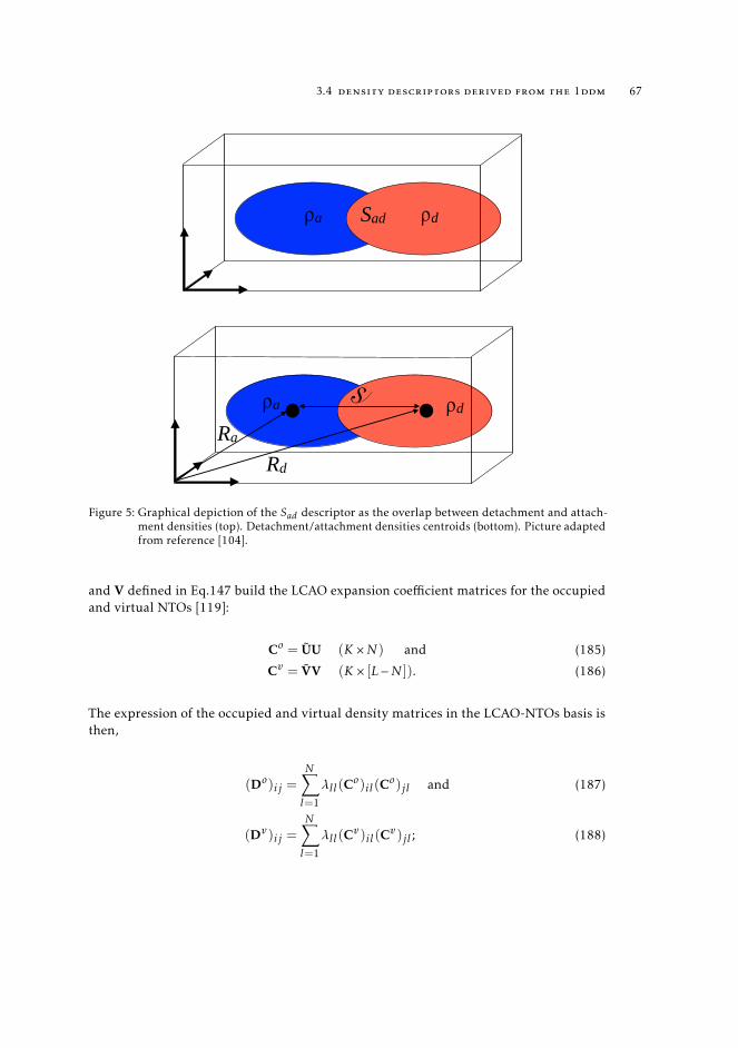
3.4 density descriptors derived from the 1ddm 67
ρa ρdSad
sRa
Rd
ρa ρd
Figure 5: Graphical depiction of the Sad descriptor as the overlap between detachment and attach-ment densities (top). Detachment/attachment densities centroids (bottom). Picture adaptedfrom reference [104].
and V defined in Eq.147 build the LCAO expansion coefficient matrices for the occupiedand virtual NTOs [119]:
Co = UU (K ×N ) and (185)
Cv = VV (K × [L−N ]). (186)
The expression of the occupied and virtual density matrices in the LCAO-NTOs basis isthen,
(Do)ij =N∑l=1
λll(Co)il(C
o)jl and (187)
(Dv)ij =N∑l=1
λll(Cv)il(C
v)jl ; (188)
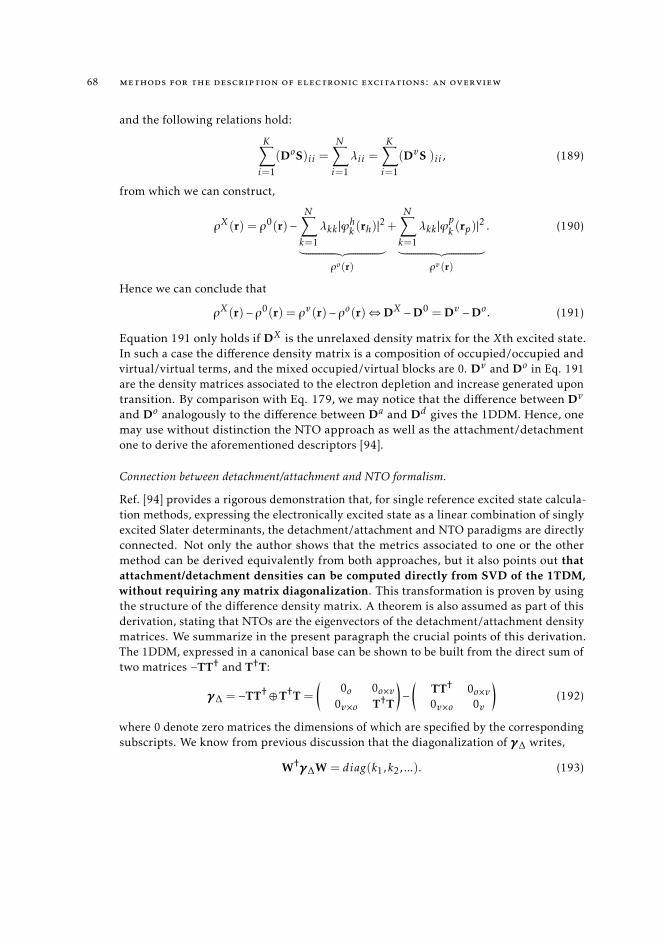
68 methods for the description of electronic excitations: an overview
and the following relations hold:
K∑i=1
(DoS)ii =N∑i=1
λii =K∑i=1
(DvS )ii , (189)
from which we can construct,
ρX (r) = ρ0(r)−N∑k=1
λkk |ϕhk (rh)|2︸ ︷︷ ︸ρo(r)
+N∑k=1
λkk |ϕpk (rp)|2︸ ︷︷ ︸ρv(r)
. (190)
Hence we can conclude that
ρX (r)− ρ0(r) = ρv(r)− ρo(r)⇔DX −D0 = Dv −Do. (191)
Equation 191 only holds if DX is the unrelaxed density matrix for the Xth excited state.In such a case the difference density matrix is a composition of occupied/occupied andvirtual/virtual terms, and the mixed occupied/virtual blocks are 0. Dv and Do in Eq. 191are the density matrices associated to the electron depletion and increase generated upontransition. By comparison with Eq. 179, we may notice that the difference between Dv
and Do analogously to the difference between Da and Dd gives the 1DDM. Hence, onemay use without distinction the NTO approach as well as the attachment/detachmentone to derive the aforementioned descriptors [94].
Connection between detachment/attachment and NTO formalism.
Ref. [94] provides a rigorous demonstration that, for single reference excited state calcula-tion methods, expressing the electronically excited state as a linear combination of singlyexcited Slater determinants, the detachment/attachment and NTO paradigms are directlyconnected. Not only the author shows that the metrics associated to one or the othermethod can be derived equivalently from both approaches, but it also points out thatattachment/detachment densities can be computed directly from SVD of the 1TDM,without requiring any matrix diagonalization. This transformation is proven by usingthe structure of the difference density matrix. A theorem is also assumed as part of thisderivation, stating that NTOs are the eigenvectors of the detachment/attachment densitymatrices. We summarize in the present paragraph the crucial points of this derivation.The 1DDM, expressed in a canonical base can be shown to be built from the direct sum oftwo matrices −TT† and T†T:
γγγ∆ = −TT† ⊕T†T =
(0o 0o×v
0v×o T†T
)−(
TT† 0o×v0v×o 0v
)(192)
where 0 denote zero matrices the dimensions of which are specified by the correspondingsubscripts. We know from previous discussion that the diagonalization of γγγ∆ writes,
W†γγγ∆W = diag(k1,k2, ...). (193)
3.4 density descriptors derived from the 1ddm 69
By construction, −TT† and T†T are positive definite [94, 103], therefore all negativeeigenvalues of γ∆ belong to the occupied × occupied block, while the positive ones stemfrom the virtual × virtual block. Therefore, the following relation hold,
TT† ⊕ 0v = γγγd∆ ; 0o ⊕T†T = γγγa∆. (194)
Besides, according to Eq.147, we know that
diag(k1,k2, ...) = −λλλo ⊕λλλv , (195)
and that the matrix W diagonalizing the 1DDM is given by:
W = U⊕V. (196)
From Eq.194 one deduces that the eigenvectors of the detachment/attachment matricesare the occupied/virtual transition orbitals. The matrices Za,Zd diagonalizing γγγ∆ write,
Za = 0o ⊕O =⇒ Za†γγγaZa = 0o ⊕λv ; Zd = O⊕ 0v =⇒ Zd†γγγdZd = λv ⊕ 0v (197)
Based on these relation Ref. [94] delineates a scheme for the joint computation of detach-ment/attachment densities from the eigenvectors and singular values of the 1TDM.
• U†TV = diag(√λ1,√λ2, ...)→ λλλo;λλλv → γγγ∆ = −UλλλoU† ⊕VλλλvV†
• according to the structure of diag(k1,k2, ...) one can express the attachment/detach-ment eigenvalues, a and d as diag(k1,k2, ...) = −λλλo⊕λλλv ⇒ a = 0o⊕λλλv ; d = 0v⊕λλλo.
• which leads to
(UUU ⊕VVV )a(UUU† ⊕VVV †) = γγγa and (UUU ⊕VVV )d(UUU† ⊕VVV †) = γγγd (198)
• from which all the desired metrics can be obtained, γγγa,γγγd → Sad ,s,sS
3.4.3 Hilbert-space related attachment/detachment density matrices-based centroids of charge
Attachment and detachment densities can be used to measure the charge displacementlength, by computing the difference between the charge centroids associated to these twodistributions. For a detailed discussion on Hilbert-space related attachment/detachmentdensity matrices-based centroids of charge we refer to references [103, 104, 106]. Just asfor the DCT which we have introduced in Section 3.4.1, one computes the centroids (Ra,Rd ) of the attachment and detachment densities as,
Rd = κ−1
∫R3dr rρd(r),= (xd ,yd ,zd) (199)
Ra = κ−1
∫R3dr rρa(r),= (xa,ya,za) (200)
70 methods for the description of electronic excitations: an overview
where κ is the total integrated attached/detached charge, defined as
κ=
∫R3dr ρξ (r). (201)
where ξ takes values of a or d. The distance between the two centroids writes,
ðCT =| Rd −Ra | . (202)
Similarly the transferred charge is given by the norm,
wτ =
∫R3dr ρτ (r) =⇒ wCT =
12
∑τ=a,d
wτ . (203)
Again, it is interesting to ponder on the difference between the ρd and ρa densities andthe ρ+ and ρ− pair. The same holds for wτ and qCT. One may notice that alternativederivations of the same quantities are possible, by employing the methodologies illustratedabove. For instance, one can extract the positive and negative density distributionsrespectively from the attached and detached densities. If we denote the charge-transferdistance and the charge displaced, calculated with this third strategy as DCT and qCT, thefollowing relations hold:
qCT ≡ qCT ≤ wCT (204)
DCT ≡ DCT ≥ ðCT, (205)
(206)
where the inequality stems from the fact that wCT incorporates a portion of overlappingdensity that cancels out in qCT, which is computed form real-space difference density.This discrepancy extends to the barycenters as well. Furthermore, we have seen in theprevious section that the three descriptors s and sS and Sad can be equivalently derivedboth using the 1DDM and the 1TDM approach. The analogous correspondence applies toqCT and DCT. As a result, the following equivalences also hold:
γγγNTOa −γγγNTO
d = γγγa −γγγd ⇒ qCT = qNTOCT ; DCT = DNTO
CT , (207)
where the superscript NTO indicates that the descriptors are obtained from SVD of the1TDM.
3.5 analysis of excited states from 1tdm
3.5.1 An orbital based descriptor: ∆r
In the previous part, we have given an overview of the latest advances regarding excitedstates descriptors derived from the 1DDM. As anticipated before, a second approachexists, based on the 1TDM. The two methods are formally connected. Specifically, for thecase of electronically excited states expressed as a linear combination of singly excited
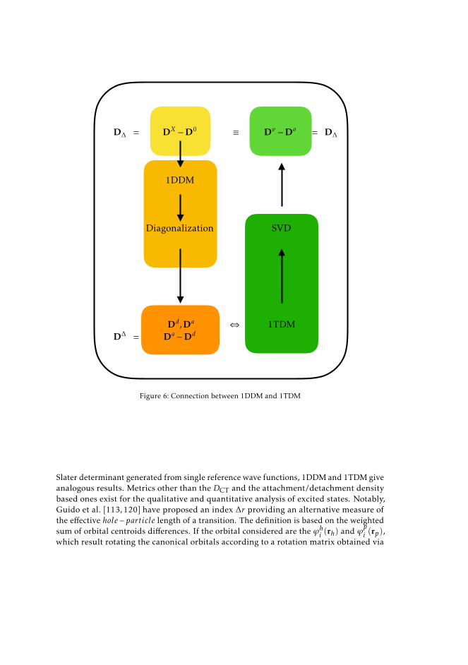
3.5 analysis of excited states from 1tdm 71
D = DX D0 Dv Do = D
1DDM
Diagonalization SVD
Dd,Da , 1TDMD = Da Dd
1
Figure 6: Connection between 1DDM and 1TDM
Slater determinant generated from single reference wave functions, 1DDM and 1TDM giveanalogous results. Metrics other than the DCT and the attachment/detachment densitybased ones exist for the qualitative and quantitative analysis of excited states. Notably,Guido et al. [113, 120] have proposed an index ∆r providing an alternative measure ofthe effective hole − particle length of a transition. The definition is based on the weightedsum of orbital centroids differences. If the orbital considered are the ϕhi (rh) and ϕ
pi (rp),
which result rotating the canonical orbitals according to a rotation matrix obtained via
72 methods for the description of electronic excitations: an overview
SVD of the 1TDM (see Eq. 144), then the maximal correspondence between excited holeand particle is obtained. The ∆r index writes,
∆r =
∑Noi λii |
⟨ϕpi (rp)
∣∣∣r ∣∣∣ϕpi (rp)⟩− ⟨ϕhi (rh)∣∣∣∣r ∣∣∣∣ϕhi (rh)⟩ |∑Noi λii
, (208)
where the⟨ϕp(h)i (rp(h)
∣∣∣∣∣r ∣∣∣∣∣ϕp(h)i (rp(h))⟩
are defined as the norm of the orbital centroids
and the λii are the singular values of the 1TDM (i.e., the eigenvalues associated to the ithhole-particle transition). Moreover to best characterize an electronic transition one wantsto give an estimate of the delocalization of the electrons around the orbital centroids.Based on this observation, the authors modified the original ∆r definition by coupling itto a measure of the particle spread around the charge centroids are given by,
σp =
√⟨ϕpi (rp)
∣∣∣r2∣∣∣ϕpi (rp)⟩− ⟨ϕpi (rp)∣∣∣r ∣∣∣ϕpi (rp)⟩2
. (209)
The two can be combined into a new metric Γ ,
Γ = ∆r +∆σ =
⟨ϕpi (rp)
∣∣∣r ∣∣∣ϕpi (rp)⟩− ⟨ϕhi (rh)∣∣∣∣r ∣∣∣∣ϕhi (rh)⟩ |∑Noi λii
+
∑Noi λii | σp − σh |∑No
i λii. (210)
In the context of TDDFT, Γ may also be used to discriminate between short and long-rangeexcitations. Given its formulation, which provides both a measure of the charge-transferdistance and of the spread of the electrons around the centroids, Γ can individuate anytransition, from valence to charge-transfer and Rydberg states. Finally, not only Γ providesa measure of the effective hole − particle distance covered during the excitations, but itsinterest also resides in the ability to render a reliable diagnostic of the performance ofTDDFT, even in those cases where other diagnostic indexes fail [121].
3.5.2 Exciton descriptors
The present discussion, although legitimate for our purposes, is certainly limited interms of the topics covered and compared to the abundance of papers devoted to excitedstates analysis. In particular, one major question we have not addressed until now, is thepossibility of including static and dynamic electronic correlation effects. These can beimportant, as there are properties that derive directly from it, for instance, electron-holebinding and exciton sizes. These, are naturally more of concern in the context of solid-state physics, which deviates quite from our focus. However, for large molecular systems,it has been shown that exciton-effects may be crucial for a correct interpretation of theelectronic excitation [31, 122–125].
Furthermore, there it has been pointed out that hole/electron pairs, generated inelectronic excitations suffer the same limits at the TDDFT level as charge-transfer statesdo [124]. In this context it is interesting to mention the work carried out by Plasser et
3.5 analysis of excited states from 1tdm 73
al. [108, 112], which offers an additional interpretation of the 1TDM which we have notyet discussed. The one-one particle difference density matrix can be interpreted as theeffective two-body exciton wave function, describing the correlated hole-particle motion.This identification is justified in Ref. [112] in term of many-body Greens-function theory.Based on this assumption, the authors propose a set of descriptors yielding a quantitativeanalysis of excited states [107, 110, 112]. The central quantity of this analysis is again the1TDM, defined in Eq. 137. The latter, is expressed in coordinate space as,
χX (rh,rp) =L∑p
L∑q
ϕp ∗ (rh)⟨Ψ 0
∣∣∣ a†paq ∣∣∣Ψ X⟩ϕq(rp) (211)
= γγγ0X (rp,rh), (212)
where rp,rh denote hole and particle coordinates, and a†p, aq annihilate the electron in ϕpand create a hole in orbital ϕq, respectively. The exciton wave function may be expressedin an even more compactly by using the NTOs.
χexc(rh,rp) =N∑i=1
√λiϕ
hi (r)ϕ
pi (r). (213)
Here ϕhi (r)ϕpi (r) are the hole and particle wave functions and the label i indexes the
orbital pair corresponding to the singular values√λi . This representation of the electronic
transition avoids the bias associated with a specific orbital choice, leading to a compactand more realistic representation of the exciton.
In summary, the theory of exciton analysis is independent of the wave function modeland provides an exact picture of the electronic excitation. Moreover, it may be applied tocalculate a variety of wave function properties, while being invariant from orbital rotationnor dependent on a partitioning of the wave function into atomic contributions [94, 112].This representation of the electronic transition avoids the arbitrariness associated with aspecific molecular orbital choice [112] leading to a sound and more rigorous descriptionof the exciton [107, 111]. The non zero singular values of the 1TDM inherently deliverthe information of the number of relevant contributions that are needed to describe theexcitation. This concept may be quantified as the participation ratio [107],
P RNTO =
∑i(λi)
2∑i λ
2i
=Ω∑i λ
2i
(214)
where Ω is the squared norm of the exciton wave function
Ω= 〈χexc| χexc〉= γ0Xγ0Xγ0X (rh,rp)2 = || γγγ0X ||2 . (215)
The P RNTO expresses the number of independent configuration needed to describe anexcitation. For wave functions other than in an unrelaxed CIS/TDA calculation, in whichcase P RNTO = 1, the latter can be considered as a estimation of the amount of singleexcitation character. A P RNTO > 1 implies that several configurations contribute to a
74 methods for the description of electronic excitations: an overview
state. Differently stated it gives a measure of the static correlation. All information carriedwithin the exciton wave function is released by calculating the expectation value of thelatter with respect to an operator of interest,
〈O〉= 〈χexc|O |χexc〉〈χexc| χexc〉
(216)
An approach to characterize exciton wave functions is to compute its spacial and statisticalproperties, which provide a measure of its broadness and delocalization in space. Thederivation of the latter relies on Eq.216 [112]. As stated by Eq. 215 the denominator is thesquared norm of the transition density matrix. Written in atomic orbital space the latterreads,
Ω= T r(D0X†SD0XS) (217)
where S, has elements Sµν , that are the atomic orbital overlaps of χµ(r),χν(r). The nu-merator can be simplified by expressing the operator as product of one particle operators,
O = h(rh)p(rp). (218)
Writing the expectation value in orbital representation leads to
h(rh)p(rp) =1Ω
K∑µ
K∑ν
K∑ζ
K∑ξ
DµνDζξ× (219)
∫R3drh χµ(rh)h(rh)χξ (rh)×
∫R3drp χnu(rp)hp(rp)χζ(rh) (220)
=1Ω
K∑µ
K∑ν
K∑ζ
K∑ξ
hµνpζξ (221)
=1ΩT r(D0X†hD0Xp) (222)
Moreover of the operators are functions of rh and rp, but do not act explicitly on holeand particle coordinates, i.e., h(rh)p(rp) = 〈f (rh,rp)〉, then the expectation value reducesto the integration of the product of a 〈f (rh,rp)〉 and the squared norm of the 1TDM. If〈f (rh,rp)〉 is a multipole matrix one can derive several relations to compute the locality ofan exciton.The size of the exciton is given by,
dexc =√〈| rh − rp |2〉. (223)
3.5 analysis of excited states from 1tdm 75
Expanding, gives
d2exc =
∑r=x,y,z
〈(rh − rp) · (rh − rp)〉exc (224)
=∑
r=x,y,z〈(rh · rh)〉exc − 〈2(rh · rp)〉exc + 〈(rp · rp)〉exc (225)
=∑
r=x,y,z〈r2h 〉exc − 〈2rh · rp〉exc + 〈r2p 〉exc. (226)
The nine terms of Eq. 226 are the expectation values of the one-electron multipoleoperators. Considering Eq. 222, these write,
〈xkhxkh〉exc =1ΩT r(DX0M
(l)x D0XM
(l)x ). (227)
The elements of M(l)x are the k-order multipole moments for component x, given as,
M(l)k ,µν =
∫R3χµ(r)x
kχν(r) (228)
The calculation of dexc reduces then to a series of matrix multiplications. The practicalequation that can be used to calculate the exciton size is:
d2exc =
1Ω
∑r=x,y,z
(T r(DX0M(2)r D0XS)− 2T r(DX0M
(1)r D0XM
(1)r ) + T r(DX0SD0XM
(2)r )).
(229)
the second order terms contain the quadrupole moments of hole density (D0XSDX0)and of the particle density (DX0SD0X ), respectively, while the first order term expressesthe mixed dipole contributions deriving from the correlated motion of the hole andparticle [112]. A complementary quantity to the exciton size is the vectorial distancebetween the centroids of the hole and particle distributions:
~dh→e = 〈rh − rp〉exc. (230)
While ~d is a measure of the linear charge transfer, dexc also incorporates the exciton chargeresonance effects. Analogously to the exciton size, one can also compute hole and particlesizes separately, as,
σh = (〈r2h 〉exc − 〈rh〉2exc)
1/2 (231)
σe = (〈r2p 〉exc − 〈rp〉2exc)
1/2 (232)
These can be related to the mean average positions 〈rh〉exc,〈rp〉exc to give an estimateof the spread of hole and particle with respect to the charge centroids. Along with thegeometrical descriptors discussed above, a statistical interpretation of the exciton has also
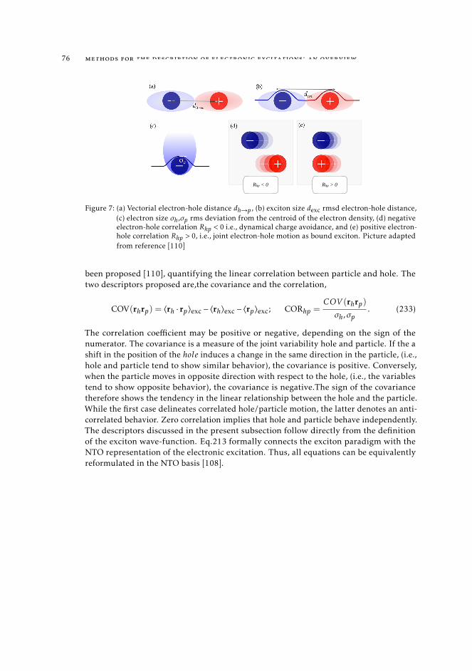
76 methods for the description of electronic excitations: an overview
Rhp < 0 Rhp > 0
Figure 7: (a) Vectorial electron-hole distance dh→p , (b) exciton size dexc rmsd electron-hole distance,(c) electron size σh,σp rms deviation from the centroid of the electron density, (d) negativeelectron-hole correlation Rhp < 0 i.e., dynamical charge avoidance, and (e) positive electron-hole correlation Rhp > 0, i.e., joint electron-hole motion as bound exciton. Picture adaptedfrom reference [110]
been proposed [110], quantifying the linear correlation between particle and hole. Thetwo descriptors proposed are,the covariance and the correlation,
COV(rhrp) = 〈rh · rp〉exc − 〈rh〉exc − 〈rp〉exc; CORhp =COV (rhrp)
σh,σp. (233)
The correlation coefficient may be positive or negative, depending on the sign of thenumerator. The covariance is a measure of the joint variability hole and particle. If the ashift in the position of the hole induces a change in the same direction in the particle, (i.e.,hole and particle tend to show similar behavior), the covariance is positive. Conversely,when the particle moves in opposite direction with respect to the hole, (i.e., the variablestend to show opposite behavior), the covariance is negative.The sign of the covariancetherefore shows the tendency in the linear relationship between the hole and the particle.While the first case delineates correlated hole/particle motion, the latter denotes an anti-correlated behavior. Zero correlation implies that hole and particle behave independently.The descriptors discussed in the present subsection follow directly from the definitionof the exciton wave-function. Eq.213 formally connects the exciton paradigm with theNTO representation of the electronic excitation. Thus, all equations can be equivalentlyreformulated in the NTO basis [108].
Part II
TDDFT ROOTED PROCEDURES FOR THE DESCR IPT ION OF
EXC ITED STATES

4EXC ITED STATES FROM TDDFT: A MEASURE OF
CHARGE -TRANSFER
4.1 context
The time-dependent response theory approach outlined in Chapter 3 provides a routeto excitation energies and transition moments. Excited state (ES) total energies arethen accessed by adding the excitation energy to the corresponding ground state (GS)energy. This methodology gives access to useful objects, such as the 1DDM, which enclosethe information related to the polarization of the electronic cloud occurring within theexcitation. Within the Time-Dependent Functional Theory (TDDFT), additionally, toimprove the description of the density matrices, one may perform a post-linear responsetreatment of the excited state calculation, by computing the so-called Z-vector [126]. Inthe TDDFT scheme, this computation results in the addition of a matrix (occupied-virtualterms) to the 1DDM to account for the density relaxation following the hole/particlegeneration. The resulting redistributed excited state density is the so-called relaxeddifference density matrix.
This procedure opens the question of how the quality of the computed densities af-fects the descriptors that are directly derived from it. This question is the focus of arecent publication of ours: “How are the charge-transfer descriptors affected by the qual-ity of the underpinning electronic density?”, by myself, Marco Campetella, Michael J.Frisch, Giovanni Scalmani, Carlo Adamo, and Ilaria Ciofini, published in the Journal ofComputational Chemistry. The present chapter constitutes an adaptation of the latterpublication.
4.2 introduction
In the recent decades, we have witnessed an intensive and increasing use of theoreticalapproaches to describe and predict excited state phenomena and properties of molecularcompounds [20, 127, 128]. Among different methods, TDDFT has emerged as one ofthe most applied, mainly due to its low cost to accuracy ratio and its simple formalism,making it widely available to both theoretical and experimental chemists’ community [19].Nonetheless, besides its numerous successes, it is nowadays well established that TDDFTapproaches have severe drawbacks that can be in large part ascribed to the quality of theunderlying density functional approximation used to describe the exchange-correlationenergy [127]. Indeed, several works pointed out that TDDFT approaches yield significanterrors when applied to the description of CT excitations, especially when local exchange-correlation functionals (such as Generalized Gradient Approximation, GGA or LocalDensity Approximation, LDA) are used [129]. More specifically, these type of functionals
79
80 excited states from tddft: a measure of charge-transfer
do not correctly recover the 1/R asymptotic behavior relevant for the description of CTstates and global or range-separated hybrid functionals, including in different ways exactHartree–Fock exchange have been often proposed as a suitable alternative to improveTDDFT performances in the description of this type of excited states [30, 121, 130].
However, if a correct description of CT phenomena is still tricky to achieve [121,131,132]the design of molecules able to give rise to CT or charge separation (CS) at the excitedstate is a flourishing experimental field due to their relevance in many fields of applicationranging from artificial photosynthesis to hybrid solar cells. The so-called push-pullsystems represent one of the most common molecular topologies, experimentally usedto generate these type of excited states. These molecular structures that are made up ofan electron-donating group (D) and acceptor group (A) covalently bound often in a rigidand rod-like fashion by a spacer, whose length and conjugation degree can be eventuallychanged to tune their properties (e.g., the absorption energy) [117, 133, 134].
These systems display at least one low lying intensively absorbing excited state withrelevant CT character and schematically corresponding to the transfer of an electron fromthe D to the A, which leads to the formation of a formal [D-A] excited state. However, inmost cases, both the excited state hole and electron are far from being strictly localizedon the donor/acceptor fragments. Depending on their chemical nature, as well as onthe bridge length, the spatial extent and the magnitude of the electron transfer can besignificantly different. As introduced in Chapter 3, many indexes have been devised inthe last years to define the nature—and eventually measure—the extent of CT excitationas well as to diagnostic the reliability of TDDFT approaches in calculating the energy andintensity of the electronic transition [117, 127, 134–136].
Among others, and for this purpose, an index, the (DCT), has been recently developedby some of us, allowing to define the spatial extent associated with a given transition,using only the density distributions of the associated ground and excited electronicstates [1]. More recently we have also proposed a new index (the MACindex) enabling toassess the degree of reliability of CT excitations has been more recently further derivedfrom the DCT by us [5]. Both these indexes are based on the evaluation of ground andexcited state densities. According to the Z-vector method [126], the TDDFT total ESdensity can be refined by applying a post-linear-response correction, which accounts forrelaxation effects [137], associated with electronic transitions, when the excited statesare calculated either in the diabatic framework or vertically. Since then, several workshave been published on the importance of the inclusion of density relaxation effects in theadiabatic framework and beyond [138–141]. As reported in the latter works, the densityvariation within the adiabatic picture - referred to as unrelaxed - differs from the diabatic -relaxed - picture by the inclusion of the effect of the charge rearrangement and the changein bond order due to the electronic excitation. Accordingly, in this contribution, we applythe same terminology.
In this work, we used a prototype push-pull system (namely the family of the α,ω-dimethylamino-nitropolyphenylene,8) to evaluate the impact of ES density relaxationon the computed density-based descriptor (i.e., the DCT index). As the CT parametersstrongly depend on the exchange-correlation functional used, we investigate such effect
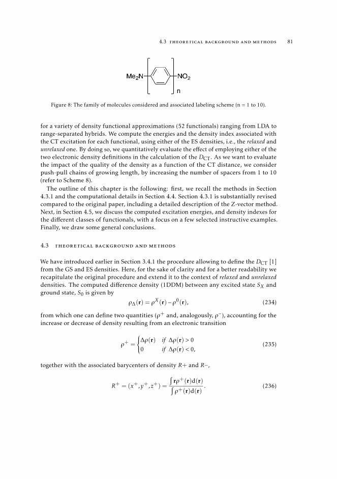
4.3 theoretical background and methods 81
Figure 8: The family of molecules considered and associated labeling scheme (n = 1 to 10).
for a variety of density functional approximations (52 functionals) ranging from LDA torange-separated hybrids. We compute the energies and the density index associated withthe CT excitation for each functional, using either of the ES densities, i.e., the relaxed andunrelaxed one. By doing so, we quantitatively evaluate the effect of employing either of thetwo electronic density definitions in the calculation of the DCT. As we want to evaluatethe impact of the quality of the density as a function of the CT distance, we considerpush-pull chains of growing length, by increasing the number of spacers from 1 to 10(refer to Scheme 8).
The outline of this chapter is the following: first, we recall the methods in Section4.3.1 and the computational details in Section 4.4. Section 4.3.1 is substantially revisedcompared to the original paper, including a detailed description of the Z-vector method.Next, in Section 4.5, we discuss the computed excitation energies, and density indexes forthe different classes of functionals, with a focus on a few selected instructive examples.Finally, we draw some general conclusions.
4.3 theoretical background and methods
We have introduced earlier in Section 3.4.1 the procedure allowing to define the DCT [1]from the GS and ES densities. Here, for the sake of clarity and for a better readability werecapitulate the original procedure and extend it to the context of relaxed and unrelaxeddensities. The computed difference density (1DDM) between any excited state SX andground state, S0 is given by
ρ∆(r) = ρX (r)− ρ0(r), (234)
from which one can define two quantities (ρ+ and, analogously, ρ−), accounting for theincrease or decrease of density resulting from an electronic transition
ρ+ =
∆ρ(r) if ∆ρ(r) > 0
0 if ∆ρ(r) < 0,(235)
together with the associated barycenters of density R+ and R−,
R+ = (x+,y+,z+) =
∫rρ+(r)d(r)∫ρ+(r)d(r)
. (236)
82 excited states from tddft: a measure of charge-transfer
The spacial distance between the two barycenters of density distributions is then used toquantify the length of the CT excitation:
DCT =| R+ −R− | . (237)
Clearly, all these quantities depend on the quality of ground and excited state densities.Recent publications have highlighted the importance of density relaxation [140, 142, 143]in the context of the analysis of electronic transitions arising from a TDDFT calculation.The question on how are the charge-transfer descriptors affected by the quality of theassociated electronic density is, therefore, strictly related to the re-distribution of theelectronic density due to the excitation process. In particular, the concept of the magnitudeof such relaxation can be better quantified by the inclusion of the Z-vector in the differencedensity matrix definition.
4.3.1 Excited state properties and the Z-vector method
The Z-vector equation can be conveniently derived using a Lagrangian formalism in thelinear response framework. This method, proposed initially by Handy and Shäfer [126]has been later applied to derive excited state gradients for CIS [144] and implemented inthe Gaussian package [145]. In a later publication by Furche and Alrichs this the Z-vectormethod has been derived explicitly for TDDFT. In the following, we review the criticalsteps of the derivation. More details can be found in the Reference [138]. The followingderivations follow the spin-orbital formulation, where all spin orbitals are considered tobe real.
Time-dependent response theory, which we have introduced in Section 2.5.3, providesa root to excited states. As mentioned previously in Section 2.5.5, within the TDDFTlinear response formulation, excitation energies are obtained as the solutions of Casidaequations (Eq. 103). It is, however, convenient to introduce an equivalent, variationalformulation, as follows. Excited states are the stationary points of the functional
G[X,Y,Ω] = 〈X,Y|Λ |X,Y〉 −Ω(〈X,Y|∆ |X,Y〉 − 1), (238)
where Ω is a real Lagrange multiplier, and the vectors
〈X,Y|=(XY
), (239)
are defined in the Hilbert space of occupied and virtual molecular orbitals. The molecularorbitals(MOs) ϕpσ (r) are solutions of the ground state spin unrestricted Kohn-Sham (KS)equations with orbital eigenvalues εpσ . As usual the indexes i,j,· · · , denote occupied,a,b,· · · , virtual and p,q,· · · generic orbitals. The MOs are expanded in the basis of atomcentered contracted Gaussians χµ(r), the expansion coefficients Cpq being stored in thecoefficient matrix C. X and Y above are the expansion coefficients of the transition, that isthe first order linear response density in terms of the ground state KS-orbitals
ρ(1)(r,r’) =12
∑iaσ
(Xiaσϕaσ (r)ϕiσ (r’) + Yiaσϕiσ (r)ϕaσ (r’)). (240)
4.3 theoretical background and methods 83
Λ and ∆ are the so called "superoperators",
Λ=
(A BB A
), ∆=
(1 00 -1
). (241)
A and B are defined from the matrix elements of the time-independent KS Hamiltonian
Aia,jb = (εa − εi)δijδab + (ia|jb) + (ia|fxc|jb) (242)
Bia,jb = (ia|jb) + (ia|fxc|jb) (243)
where the integrals are expressed in Mulliken notation. A and B are generally referred toas the orbital rotation Hessians. Their matrix representation writes,
(A+B)iaσjbσ ′ = (εaσ − εiσ )δijδabδσσ ′ + 2(iaσ |jbσ ′) + 2f xciaσjbσ ′
− cxδσσ ′ [(jaσ |ibσ ) + (abσ |ijσ )], (244)
(A−B)iaσjbσ ′ = (εaσ − εiσ )δijδabδσσ ′ + cxδσσ ′ [(jaσ |ibσ )− (abσ |ijσ )] (245)
where f xcpqσrsσ ′ is the exchange-correlation kernel in the adiabatic approximation.
f xcσσ ′ (r,r’) =
δ2Exc
δρσ (r)δρσ ′ (r’)(246)
Exc denotes the exchange-correlation energy functional, that is evaluated at the groundstate energy. Then, the Lagrangian G may be expressed in the form,
G[X,Y,Ω] =12
[(X+Y)†(A+B)(X+Y)(X−Y)†(A−B)(X−Y)
]+
Ω
2
[(X+Y)†(X−Y) + (X−Y)†(X+Y)− 2
]. (247)
By applying the variational principle one obtains the stationarity conditions for G,
∂G
∂(X + Y )iaσ=
∑jbσ ′
(A+B)iaσjbσ ′ (X + Y )jbσ ′ −Ω(X −Y )iaσ = 0, (248)
∂G
∂(X −Y )iaσ=
∑jbσ ′
(A−B)iaσjbσ ′ (X −Y )jbσ ′ −Ω(X + Y )iaσ = 0, (249)
∂G∂Ω
=∑iaσ
(X + Y )iaσ (X −Y )iaσ = 0. (250)
These conditions yield the original linear response equation and the normalization condi-tions for the coefficients X,Y .
Eq. 248,249,250 are evaluated at a chosen stationary point (X,Y),Ω. As a result oneobtains a specific excitation energy Ω and transition densities (X+Y) and (X−Y).
84 excited states from tddft: a measure of charge-transfer
Once excitation energies are computed, one may compute excited state properties bythe first-order derivation of the energy with respect to an external perturbation. Thetotal electronic energy is the sum of the ground state and the excitation energy. Byanalogy, the excited state properties are a sum of the corresponding ground state andexcitation parts, where the latter is simply the derivative of the excitation energies. Theseobservations are a direct consequence of the Hellman-Feynman theorem (which specifieshow to compute the derivative of the energy of a bound state with respect to a parameterin the Hamiltonian in terms of the expectation values of the operator) and more generallyof the Wigner 2n+ 1 rule. The latter states that that the (2n+ 1)th order properties canbe evaluated from a knowledge of the wavefunction through nth order. If one denotes anexternal perturbation as ξ, one may write
Ωξ = Gξ [X,Y,Ω] = 〈X,Y|Λξ |X,Y〉 . (251)
It is interesting to note that due to the variational principle, first-order properties donot require the computation of the derivatives of the excitation vectors, (which are zeroby definition, as they are stationary points of G). However calculating Λξ still involvesthe derivatives of the MO coefficients, expressed as linear combination of atom centeredfunctions,
ϕpσ (r) =∑µ
Cpσµχµ(r). (252)
If we denote as ε the number of nuclear degrees of freedom in a single molecule, thencomputing the derivatives of the MOs would involve ε perturbations, and would betherefore ε time more demanding than computing unperturbed MOs. Luckily, it aspointed out before [138], [139], [32, chapter 16], it is possible to avoid the computation ofthe derivatives of Cξ . This is possible by introducing the so-called “relaxed” densities,which in turn allow computing excited state properties at a computational cost that isindependent of ε. The Lagrangian of the excitation energy can be expressed [138] as,
L[X,Y,Ω,C,Z,W] = 〈X,Y|Λ |X,Y〉 −Ω(〈X,Y|∆ |X,Y〉 − 1) +∑iaσ
Fiaσ −∑pqσ
Wpqσ (Spqσ − δpq).
(253)
Spqσ are the overlap integrals of the KS orbitals. The matrix elements Fiaσ are obtainedby replacing the diagonal part of (A + B) and (A − B) in equations 244 and 245 byFabσδij − Fijσδabδσσ ′ . The effective KS one particle Fock operator comprises the usualterms, that are the core Hamiltonian h, a Coulomb and exchange part, and the exchange-correlation potential respectively,
Fpqσ = hpqσ +∑iσ ′
[(pqσ |iiσ ′)− cxδσσ ′ (piσ |iqσ ) +V xcpqσ ] (254)
V xcσ =
δExc
δρσ (r)(255)
4.3 theoretical background and methods 85
The introduction of F is particularly appropriate: by construction F is diagonal, witheigenvalues εpσ on the diagonal. This substitution renders the excited state formalisminvariant under any unitary transformation of occupied and virtual orbitals since allphysical properties are invariant under the same transformations. These conditions isreinforced by requiring the Lagrangian L to be stationary with respect to all its parameters,X,Y,Ω,C and W. Hence the summation of the GS Lagrangian and L provides a fullyvariational root to excited state energies.
The variation of L with respect to |X,Y〉 and Ω lead back to Eqs. 248,249 and 250,while the Lagrange multipliers Ziaσ and Wpqσ introduce N2 constraints in the variationof G. As a result, the KS MOs are constrained to satisfy the KS equations and to remainorthonormal [138], for ξ , 0. Thus, the MO coefficients are fixed and Z and W can bedetermined using the stationarity of L with respect to the expansion coefficients Cµpσ ,
∂L∂Cµpσ
= 0. (256)
The expression for Ziaσ , known as Z-vector equation, writes,∑jbσ ′
(A+B)iaσjbσ ′Zjbσ ′ = −Riaσ . (257)
The right hand side of Eq. 257 takes the form,
Riaσ =∑b
[(X + Y )ibσH
+abσ [X+Y]− (X −Y )ibσH−abσ [X−Y]
−∑j
(X + Y )jaσH
+jiσ [X+Y]− (X −Y )jaσH−hiσ [X−Y]
+H+
iaσ [PU∆ ] + 2
∑jbσ ′kcσ ′′
giaσjbσ ′kcσ ′′ (X + Y )jbσ ′ (X + Y )kcσ ′′ , (258)
where gxcpqσrsσ ′tuσ ′′ is third order functional derivative matrix element,
gxcσ ′σ ′σ ′′ (r,r’,r”) =
δ3Exc
δρσ (r)δρσ ′ (r’)δρσ ′′ (r”). (259)
The operators H+ and H− are linear rotation operators which transform the differencedensity, determining the relaxation. The results of these operators acting on a arbitraryvectors - Vpqσ are,
H+pqσ [V ] =
∑rsσ ′
2(pqσ |rsσ ′) + 2f xc
pqσrsσ ′ − cxδσσ ′[(psσ |rqσ )(prσ |sqσ )
]Vrsσ (260)
H−pqσ [V ] =∑rsσ ′
cxδσσ ′[(psσ |rqσ )− (prσ |sqσ )
]Vrsσ . (261)
86 excited states from tddft: a measure of charge-transfer
The unrelaxed difference density matrix PU∆ containing the products of the excitationvectors is defined as:
Pabσ =12
∑i
(X + Y )iaσ (X + Y )ibσ + (X −Y )iaσ (X −Y )ibσ
, (262)
Pijσ = −12
∑a
(X + Y )iaσ (X + Y )jaσ + (X −Y )iaσ (X −Y )jaσ , (263)
Paiσ = Piaσ . (264)
In the MO basis, PU∆ is a symmetric matrix with both occupied-occupied (OO) and virtual-virtual (VV ) contributions only, all occupied-virtual (OV ) elements being zero. Once theZ-vector equation (Eq. 257) is solved, the relaxed one-particle difference density matrix P R∆is obtained by adding the matrix Z to the unrelaxed difference density matrix PU∆ . P R∆ will
have exactly the same OO and VV contributions as PU∆ , but the OV terms are not all zero.The appearance of these off-diagonal block elements in the excited-state density matrixcan be interpreted as orbital relaxation following the initial gross charge rearrangementdue to excitation.
P R∆ = PU∆ +Z. (265)
The information contained in P R∆ integrates that provided by the transition vector. Whilethe latter is related to the matrix elements between the ground state and the excited states,P R∆ accounts for the difference of expectation value between excited and ground states. For
example, tr(P R∆ ξ) is the change of an electron-dependent property upon excitation from
the ground state. The summation of the ground state density matrix and P R∆ returnsthe excited state properties. Population analysis of P allows for an intuitive illustrationof the charge redistribution induced by an electronic excitation. Relaxed and unrelaxeddensities, as defined above, can be used to evaluate the DCT and yield the correspondingindexes RDCT and UDCT. The former reflects the spatial extent associated to a giventransition, where the electronic density is allowed to gradually change and adapt tothe final configuration, while the latter reproduces the CT distance, measured directlyupon vertical excitation. In other words, the relaxed (RDCT), unlike its unrelaxed (UDCT)counterpart accounts for the redistribution of the electronic charge due to the excitation.
It is worth to add a couple of remarks as a conclusion to the derivation reported above.The Lagrangian in Eq. 253 is an explicit functional of any external perturbation. Thisexpedient substantially simplifies the task of calculating excited state properties, and withit, the obtainment of relaxed and unrelaxed densities. Once the X,Y,Ω,C,Z,W have beendetermined from stationarity conditions, derivatives of the excitation energy follow as,
Ωξ = Lξ [X,Y,Ω,C,Z,W] (266)
= G(ξ)[X,Y,Ω] +∑iaσ
ZiaσF(ξ)iaσ −
∑pqσ ,p5
WpqσS(ξ)pqσ . (267)
A complete mathematical treatment of the set of equations leading to excited state proper-ties falls beyond our scopes, here. However, the equations to determine the matrix W are
4.4 computational details 87
given explicitly in Ref. [139]). The reduced complexity of equation 267 (compared to eq.251) lies in the fact that the derivatives can be computed easily, without need to recomputeMO coefficients that are kept at their zero values, as indicated by the superscripts (ξ).
4.4 computational details
In this study, we have tested the 52 different functionals to evaluate the DCT parameters(relaxed and unrelaxed), for push-pull dyes of increasing length. We calculated a seriesof α,ω-NMe2,NO2-push-pull systems, varying the number of phenyl rings in the chainfrom one to ten. The geometries were built such that the phenyl rings are 45° orientedone towards the other. All calculations were performed using the development version ofthe Gaussian suite of programs [145]. Optimized in vacuum GS structural parameterswere determined for each functional, where an SCF energy convergence criterion of 10−8
a.u. was applied; the maximum SCF cycle number was set to 500, and the QC option wasspecified to prevent convergence failure problems. Frequency calculations indicated thatall optimized structures correspond to minima. The optimized structures were proven toretain a linear shape. Gas-phase vertical excitation energies were computed by TDDFTcalculations, on top of each optimized geometry. The 6-311G(d,p) atomic basis set wasused both for the ground- and excited-sate calculations. Besides, we performed CISreference calculations at the same level of theory.
The benchmark includes a broad variety of functionals taken from different classes,(the complete list is reported in Table 2). As for the local density functionals we testedthe performance of the SVWN [35, 37, 74]. Furthermore, the performance of a numberof GGA and mGGA functionals, namely BLYP [48, 55], BPBE [43, 55], BP86 [49, 55],BPW91 [50,55], B97D [52], OLYP [48,69], MPWP86 [49,67], MPWPW91 [50,67], MPWLYP[48, 67], HCTH [57], HCTH407 [57], PBE [43], PBEPW91 [43, 50], PW91PW91 [50],SOGGA11 [72], BMK [54], M06L [62], M11L [65], TPSSTPSS [44], VSXC [77], tHCTH[75] was tested. Along with the former we report the performance of a number ofglobal hybrid-GGA and -mGGA functionals, B1LYP [45, 48], B1B95 [47], B3LYP [45, 48],B3PW91 [45,50], B3P86 [45,49], B98 [51], BHandHLYP [53], HFPW91 [50], O3LYP [48,70],mPW1PW [67], PBE0 [46], SOGGA11X [73], M05 [59], M06 [26], M052X [60], M062X [26],M06HF [63], M08HX [61], TPSSh [76], tHCTHhyb [75], for improved charge transferdescription. Finally we included the Range Separated Hybrids (RSH) CAM-B3LYP [56],HSEH1PBE [146], N12SX [68], wB97 [78], wB97X [78], wB97XD [79]and M11 [64],the long range corrected LC-PBE [58] and the Non separable Gradient Approximation(NGA) functionals MN12L [68], N12 [68].
4.5 on the nature of the first excited state of push-pull molecules of
various length
α,ω-Amino,nitro-polyphenylene molecules (Scheme 8 are a prototype family of push-pullsystems for which the energy and nature of the first excited strongly depends on thelength of the spacer that connects the electron donor (D, here an amino group NH2) and
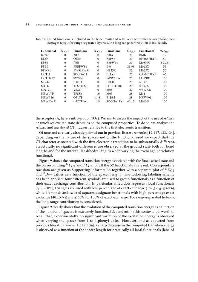
88 excited states from tddft: a measure of charge-transfer
Table 2: Listed functionals included in the benchmark and relative exact exchange-correlation per-centages (cHF , (for range separated hybrids, the long range contribution is indicated).
Functional % cHF Functional % cHF Functional % cHF Functional % cHFB97D 0 N12 0 B3LYP 20 BMK 42BLYP 0 OLYP 0 B3P86 20 BHandHLYP 50BP86 0 PBE 0 B3PW91 20 M08HX 52.23BPBE 0 PBEPW91 0 B98 21.98 M062X 54BPW91 0 PW91PW91 0 N12SX 25 M052X 56HCTH 0 SOGGA11 0 B1LYP 25 CAM-B3LYP 65HCTH407 0 SVWN 0 mPW1PW 25 LC-PBE 100M06L 0 tHCTH 0 PBE0 25 wB97 100M11L 0 TPSSTPSS 0 HSEH1PBE 25 wB97X 100MN12L 0 VSXC 0 M06 27 wB97XD 100MPWLYP 0 TPSSh 10 M05 28 M11 100MPWP86 0 O3LYP 11.61 B1B95 28 HFPW91 100MPWPW91 0 tHCTHhyb 15 SOGGA11X 40.15 M06HF 100
the acceptor (A, here a nitro group, NO2). We aim to assess the impact of the use of relaxedor unrelaxed excited state densities on the computed properties. To do so, we analyze therelaxed and unrelaxed CT indexes relative to the first electronic transition.
Of note and as clearly already pointed out in previous literature works [19,117,133,134],depending on the nature of the spacer and on the functional used we expect that theCT character associated with the first electronic transition to be substantially different.Structurally no significant differences are observed at the ground state both for bondlengths and for the interanular dihedral angles when varying the exchange-correlationfunctional.
Figure 9 shows the computed transition energy associated with the first excited state andthe corresponding UDCT and RDCT for all the 52 functionals analyzed. Correspondingraw data are given as Supporting Information together with a separate plot of UDCTand RDCT values as a function of the spacer length. The following labeling schemehas been applied: four different symbols are used to group functionals as a function oftheir exact exchange contribution. In particular, filled dots represent local functionals(cHF = 0%), triangles are used with low percentage of exact exchange (1% ≤ cHF ≤ 40%),while diamonds and twisted squares designate functionals with high percentage exactexchange (40.15% ≤ cHF ≤ 65%) or 100% of exact exchange. For range-separated hybrids,the long-range contribution is considered.
Figure 9 clearly shows that the evolution of the computed transition energy as a functionof the number of spacers is extremely functional dependent. In this context, it is worth torecall that, experimentally, no significant variation of the excitation energy is observedwhen varying the spacer from 1 to 4 phenyl units. However, and as expected fromprevious literature works [1,117,134], a sharp decrease in the computed transition energyis observed as a function of the spacer length for practically all local functionals (labeled

4.5 on the nature of the first excited state of push-pull molecules of various length 89
with dots in Figure 9 ) such as LDA and GGAs: namely SVWN, B97D, BLYP, BP86, BPBE,BPW91, HCTH407, HCTH, MPWLYP, MPWP86, MPWPW91, OLYP, PBE, PBEPW91,PW91, SOGGA11. These functionals all converge to shallow transition energy (of theorder of 978–1120 nm) for the most extended bridge unit. Qualitatively the same behavioris observed for functionals containing low percentage (i.e., below 40%) of exact exchangelabeled with triangles in Figure 9 (namely B1B95, B1LYP, B3LYP, B3P86, B3PW91, B98,mPW1PW, O3LYP, PBE0, M05, M06, tHCTHhyb, TPSSh, HSEH1PBE, and N12SX) throughthe predicted transition energy for the longest -10 units- bridge is slightly higher, rangingfrom 412 nm for the M05 functional to 658 nm for the tHCTHhyb functional.
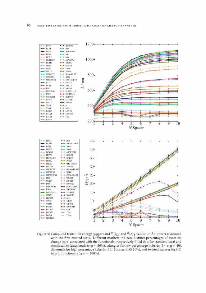
90 excited states from tddft: a measure of charge-transfer
1 2 3 4 5 6 7 8 9 10N Spacer
200
400
600
800
1000
1200
λ /
nm
B97DBLYPBP86BPBEBPW91HCTH407HCTHM06LM11LMN12LMPWLYPMPWP86MPWPW91N12OLYPPBEPBEPW91PW91SOGGA11SVWNtHCTHTPSSVSXCB1B95B1LYPB3LYPB3P86
B3PW91B98HSEH1PBEM05M06mPW1PWN12SXO3LYPPBE0TPSShBHandHLYPBMKCAM-B3LYPM052XM062XM08HXSOGGA11XtHCTHhybHFPW91LC-PBEM06HFM11wB97wB97XwB97XDCIS
1 2 3 4 5 6 7 8 9 10N Spacer
0
5
10
15
20
25
30
35
40
45
DC
T/A
B97DBLYPBP86BPBEBPW91HCTHHCTH407M06LM11LMN12LMPWLYPMPWP86MPWPW91N12OLYPPBEPBEPW91PW91SOGGA11SVWNtHCTHTPSSVSXCB1B95B1LYPB3LYPB3P86B3PW91
B98HSEH1PBEM05M06mPW1PWN12SXO3LYPPBE0tHCTHhybTPSShBHandHLYPBMKCAM-B3LYPM052XM062XM08HXSOGGA11XHFPW91LC-PBEM06HFM11wB97wB97XwB97XDCISRDCT
UDCT
Figure 9: Computed transition energy (upper) and UDCT and RDCT values (in Å) (lower) associatedwith the first excited state. Different markers indicate distinct percentages of exact ex-change (cHF) associated with the functionals: respectively filled dots for standard local andsemilocal xc functionals (cHF ≤ 50%), triangles for low percentage hybrids (1 ≤ cHF ≤ 40),diamonds for high percentage hybrids (40.15 ≤ cHF ≤ 65 50%), and twisted squares for fullhybrid functionals (cHF = 100%).
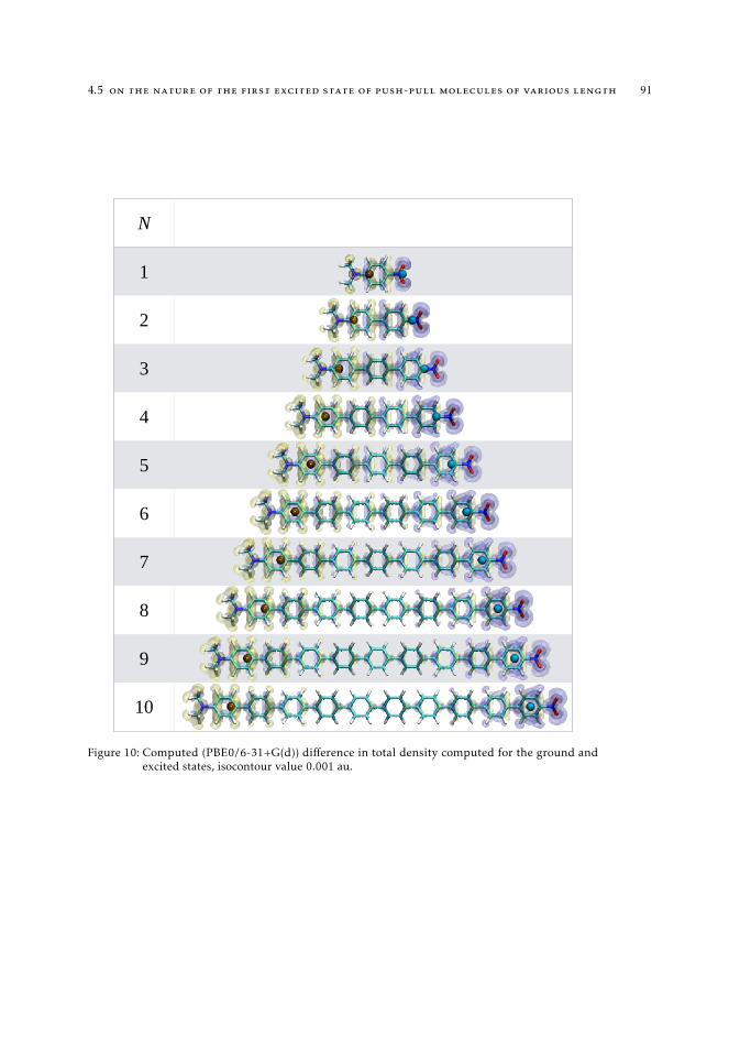
4.5 on the nature of the first excited state of push-pull molecules of various length 91
N
1
2
3
4
5
6
7
8
9
10
Figure 10: Computed (PBE0/6-31+G(d)) difference in total density computed for the ground andexcited states, isocontour value 0.001 au.
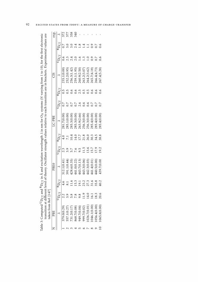
92 excited states from tddft: a measure of charge-transfer
Tabl
e3:
Com
pu
ted
UD
CT
and
RD
CT
inÅ
and
exci
tati
onw
avel
engt
hλ
innm
for
ON
syst
ems
(Nva
ryin
gfr
om1
to10
),fo
rth
efi
rst
elec
tron
ictr
ansi
tion
atd
iffer
ent
leve
lof
theo
ry.O
scil
lato
rst
ren
gth
valu
esre
lati
veto
each
tran
siti
onar
ein
brac
kets
.Exp
erim
enta
lval
ues
are
take
nfr
omR
ef.[
147]
NP
BE
PB
E0
LC-P
BE
CIS
exp
.
λU
DC
TR
DC
Tλ
UD
CT
RD
CT
λU
DC
TR
DC
Tλ
UD
CT
RD
CT
λ
137
9.0(
0.29
)2.
24.
631
2.1(
0.41
)2.
34.
028
1.7(
0.00
)0.
70.
523
5.1(
0.00
)0.
60.
737
22
557.
1(0.
27)
3.9
8.1
391.
1(0.
44)
3.9
7.1
285.
1(0.
00)
0.7
0.5
252.
2(0.
95)
2.3
3.0
377
373
1.2(
0.17
)5.
811
.642
8.6(
0.35
)5.
710
.428
5.3(
0.00
)0.
70.
625
6.3(
1.42
)2.
43.
035
84
868.
7(0.
08)
7.8
15.3
441.
0(0.
22)
7.6
14.0
285.
3(0.
00)
0.7
0.6
259.
1(1.
95)
2.0
2.4
340
594
9.7(
0.04
)9.
819
.144
3.7(
0.13
)9.
517
.726
3.9(
2.66
)2.
62.
526
0.9(
2.50
)1.
61.
8-
699
9.7(
0.02
)11
.923
.244
3.3(
0.06
)11
.521
.825
6.3(
0.00
)0.
60.
526
3.2(
3.07
)1.
31.
4-
710
26.7
(0.0
1)14
.027
.344
2.3(
0.03
)13
.626
.025
6.3(
0.00
)0.
60.
526
4.2(
3.62
)1.
01.
1-
810
46.1
(0.0
0)16
.131
.644
1.4(
0.01
)15
.730
.328
5.4(
0.00
)0.
70.
626
5.7(
4.18
)0.
90.
9-
910
56.4
(0.0
0)18
.335
.844
0.5(
0.00
)17
.934
.528
5.4(
0.00
)0.
70.
626
6.4(
4.73
)0.
70.
7-
1010
65.8
(0.0
0)20
.640
.243
9.7(
0.00
19.2
38.8
285.
4(0.
00)
0.7
0.6
267.
4(5.
28)
0.6
0.6
-
4.5 on the nature of the first excited state of push-pull molecules of various length 93
This qualitatively and quantitatively wrong prediction is related to the erratic asymptoticbehavior of the exchange-correlation functional used, as already pointed out in severalprevious works [5,20,148], giving rise to a low lying (dark) state of CT nature. Indeed, theanalysis of the corresponding UDCT indexes, computed for all local functionals, (in Figure9), suggests that all these approaches predict a transition of CT character as the lowestexcitation. Specifically, the electron displacement occurs from the HOMO (localizedon the donor group) to the LUMO (centered on the acceptor unit), with an associatedcharge-transfer distance ranging from 5 Å to 40 Å as a function of the number of spacerunits. In this case, the predicted CT distances are not very different from the geometricaldistance between the D and the A groups and increase practically linearly with the bridgelength. Indeed, the distance between the nitrogen atoms of the amino and nitro groupsranges from 5.5 Å (for N=1) to 44.1 Å (for N=10). The difference observed between thegeometrical D–A distance and the computed UDCT index is related to the conjugation ofboth the donor and the acceptor to the bridge units implying a partial delocalization ofboth HOMO and LUMO on the bridge. The DCT is directly measured from the positiveand negative barycenters of charge, which, in the case of HOMO–LUMO excitations arealways placed along the π-bridge rather than on the D/A moieties at edges of the molecule.For the sake of clarity in Figure 10 we reported a graphical representation of the positiveand negative barycenters of charge, together with the difference density plot for eachcompound, computed at the PBE0 level.
Not surprisingly, the relaxation of the excited state density strongly impacts the com-puted CT distance, especially in the case of large hole-electron separation. Indeed, thelargest RDCT values (around 20 Å) are practically half of the corresponding UDCT ones(around 40 Å). Of note, the effect of relaxation increases as a function of the effectiveCT distance so that, overall, a linear increase in the computed RDCT as a function of thespacer is still found, though with a smaller increase per spacer unit (18.3 Å for the RDCTcompared to 34.6 Å for the UDCT at the PBE level). These general observations both onthe nature of the electronic transitions and on the effect of relaxation on the computed CTdistance also holds for functionals possessing low (below 40%) exact like exchange (allrepresented as triangles in Figure 9).
In this case, although the predicted energies are not as strongly affected as for localfunctionals by the bridge length, a strong CT character is computed for all molecules withassociated CT distances not very different from those computed for the correspondingGGA functionals. This behavior can be easily spotted by comparing the transition energies,UDCT and RDCT computed at PBE and PBE0 (25% of exact-like exchange) as reported inTable 3. Also, in this case, the relaxation of the excited state density determines an extremevariation of the associated DCT value, with a RDCT value significantly smaller than theUDCT values and their difference linearly increasing with the CT length. Overall, we canthus conclude that as soon as the CT distance is more extensive than 5 Å, one observessubstantial differences between the computed UDCT and RDCT so that estimation ofquantities from the UDCT values could be affected by substantial errors.
When using hybrid functionals, with exchange contribution greater than 40% thesituation becomes more involved. Here, we focus on the behavior of three global hybrids of
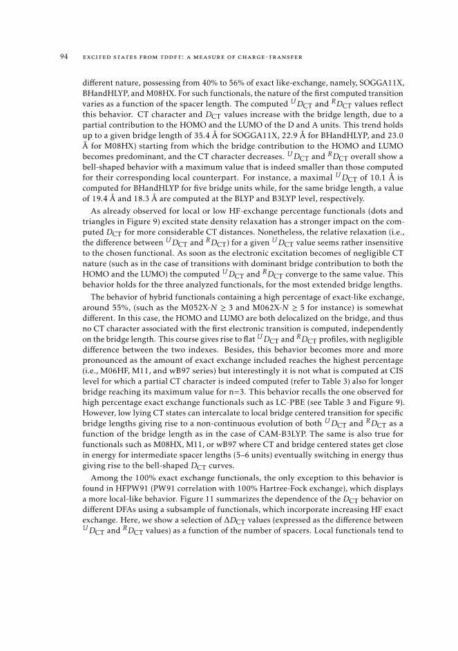
94 excited states from tddft: a measure of charge-transfer
different nature, possessing from 40% to 56% of exact like-exchange, namely, SOGGA11X,BHandHLYP, and M08HX. For such functionals, the nature of the first computed transitionvaries as a function of the spacer length. The computed UDCT and RDCT values reflectthis behavior. CT character and DCT values increase with the bridge length, due to apartial contribution to the HOMO and the LUMO of the D and A units. This trend holdsup to a given bridge length of 35.4 Å for SOGGA11X, 22.9 Å for BHandHLYP, and 23.0Å for M08HX) starting from which the bridge contribution to the HOMO and LUMObecomes predominant, and the CT character decreases. UDCT and RDCT overall show abell-shaped behavior with a maximum value that is indeed smaller than those computedfor their corresponding local counterpart. For instance, a maximal UDCT of 10.1 Å iscomputed for BHandHLYP for five bridge units while, for the same bridge length, a valueof 19.4 Å and 18.3 Å are computed at the BLYP and B3LYP level, respectively.
As already observed for local or low HF-exchange percentage functionals (dots andtriangles in Figure 9) excited state density relaxation has a stronger impact on the com-puted DCT for more considerable CT distances. Nonetheless, the relative relaxation (i.e.,the difference between UDCT and RDCT) for a given UDCT value seems rather insensitiveto the chosen functional. As soon as the electronic excitation becomes of negligible CTnature (such as in the case of transitions with dominant bridge contribution to both theHOMO and the LUMO) the computed UDCT and RDCT converge to the same value. Thisbehavior holds for the three analyzed functionals, for the most extended bridge lengths.
The behavior of hybrid functionals containing a high percentage of exact-like exchange,around 55%, (such as the M052X-N ≥ 3 and M062X-N ≥ 5 for instance) is somewhatdifferent. In this case, the HOMO and LUMO are both delocalized on the bridge, and thusno CT character associated with the first electronic transition is computed, independentlyon the bridge length. This course gives rise to flat UDCT and RDCT profiles, with negligibledifference between the two indexes. Besides, this behavior becomes more and morepronounced as the amount of exact exchange included reaches the highest percentage(i.e., M06HF, M11, and wB97 series) but interestingly it is not what is computed at CISlevel for which a partial CT character is indeed computed (refer to Table 3) also for longerbridge reaching its maximum value for n=3. This behavior recalls the one observed forhigh percentage exact exchange functionals such as LC-PBE (see Table 3 and Figure 9).However, low lying CT states can intercalate to local bridge centered transition for specificbridge lengths giving rise to a non-continuous evolution of both UDCT and RDCT as afunction of the bridge length as in the case of CAM-B3LYP. The same is also true forfunctionals such as M08HX, M11, or wB97 where CT and bridge centered states get closein energy for intermediate spacer lengths (5–6 units) eventually switching in energy thusgiving rise to the bell-shaped DCT curves.
Among the 100% exact exchange functionals, the only exception to this behavior isfound in HFPW91 (PW91 correlation with 100% Hartree-Fock exchange), which displaysa more local-like behavior. Figure 11 summarizes the dependence of the DCT behavior ondifferent DFAs using a subsample of functionals, which incorporate increasing HF exactexchange. Here, we show a selection of ∆DCT values (expressed as the difference betweenUDCT and RDCT values) as a function of the number of spacers. Local functionals tend to
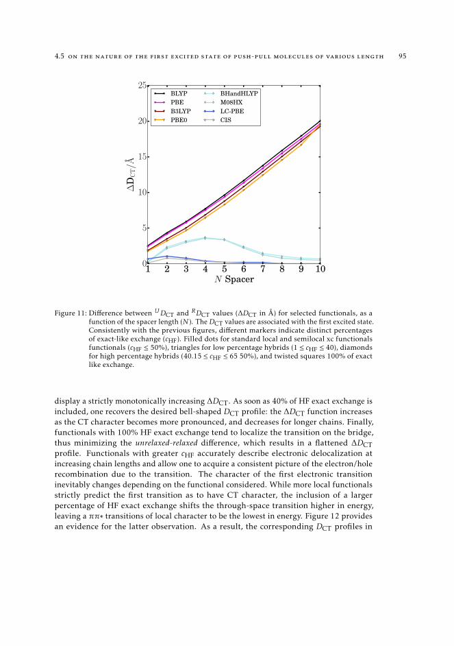
4.5 on the nature of the first excited state of push-pull molecules of various length 95
1 2 3 4 5 6 7 8 9 10N Spacer
0
5
10
15
20
25
∆D
CT/A
BLYPPBEB3LYPPBE0
BHandHLYPM08HXLC-PBECIS
Figure 11: Difference between UDCT and RDCT values (∆DCT in Å) for selected functionals, as afunction of the spacer length (N ). TheDCT values are associated with the first excited state.Consistently with the previous figures, different markers indicate distinct percentagesof exact-like exchange (cHF). Filled dots for standard local and semilocal xc functionalsfunctionals (cHF ≤ 50%), triangles for low percentage hybrids (1 ≤ cHF ≤ 40), diamondsfor high percentage hybrids (40.15 ≤ cHF ≤ 65 50%), and twisted squares 100% of exactlike exchange.
display a strictly monotonically increasing ∆DCT. As soon as 40% of HF exact exchange isincluded, one recovers the desired bell-shaped DCT profile: the ∆DCT function increasesas the CT character becomes more pronounced, and decreases for longer chains. Finally,functionals with 100% HF exact exchange tend to localize the transition on the bridge,thus minimizing the unrelaxed-relaxed difference, which results in a flattened ∆DCTprofile. Functionals with greater cHF accurately describe electronic delocalization atincreasing chain lengths and allow one to acquire a consistent picture of the electron/holerecombination due to the transition. The character of the first electronic transitioninevitably changes depending on the functional considered. While more local functionalsstrictly predict the first transition as to have CT character, the inclusion of a largerpercentage of HF exact exchange shifts the through-space transition higher in energy,leaving a ππ∗ transitions of local character to be the lowest in energy. Figure 12 providesan evidence for the latter observation. As a result, the corresponding DCT profiles in
96 excited states from tddft: a measure of charge-transfer
0 20 40 60 80 100%cHF
0
5
10
15
20
25
RD
CT/A
N = 1N = 4N = 7N = 10
0 20 40 60 80 100%cHF
0
10
20
30
40
50
UD
CT/A
N = 1N = 4N = 7N = 10
Figure 12: UDCT and RDCT for the first electronic transition against cHF percentage, for selectedspacer lengths (N = 1,4,7,10). All 53 functionals are included. Three different regimesappear clearly. Functionals including a low percentage of HF exact exchange display aconstant behavior, independently from the spacer length. An opposite behavior is foundfor full hybrid functionals (cHF = 100%). Long chains mostly display very small DCTcharacter, while only short chains have a first transition of charge-transfer character. Highpercentage hybrids (40.15 ≤ cHF, as well tend to display the same behavior.
Figure 13 representing the evolution of the lowest CT state display the desired bell-shapedprofile. Therefore, the combined uses of UDCT and RDCT can be used a first indicator ofCT pathologic cases for DFT. In particular, from Figure 11 and 13 we may deduce thatmonotonically increasing ∆DCT curves are evidence of an unphysical and erratic CT stateassociated with local exchange-correlation functionals. By contrast, for asymptoticallycorrected functionals the difference between the two indexes diminishes as the transitionchanges its nature from a HOMO-LUMO to a ππ∗ state.
4.6 conclusions
The impact of the use of relaxed or unrelaxed excited state density for the estimation of thenature and characteristic of electronically excited states with a recently developed density-based index (DCT) has been assessed using a family of prototype push-pull molecules astest case, and employing 52 different exchange-correlation density functionals belongingto different density functional classes. The following general conclusions can be drawn:
• For a qualitative description UDCT and RDCT provide the same description re-gardless of the nature (CT or not) of the transition analyzed. Thus, to characterizethe nature of electronic transitions, the associated UDCT (which can be computedon-the-fly, without any additional computational cost) can be safely used.
• For a quantitative description, UDCT and RDCT provide similar values only in thecase of transitions with moderate CT length (corresponding to distances around 4–5Å). For transition with higher CT values, the use of RDCT is warmly recommended.
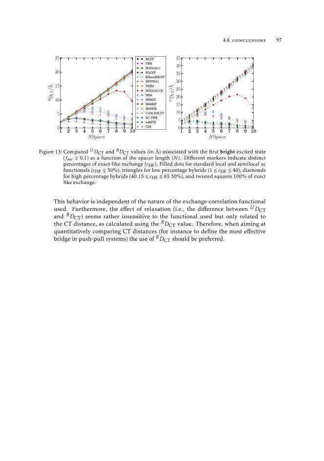
4.6 conclusions 97
1 2 3 4 5 6 7 8 9 10NSpacer
0
5
10
15
20
25
RD
CT/A
1 2 3 4 5 6 7 8 9 10NSpacer
0
5
10
15
20
25
30
35
40
45
UD
CT/A
BLYPPBESOGGA11B3LYPBHandHLYPHFPW91PBE0SOGGA11XM06M062XM06HFM08HXCAM-B3LYPLC-PBEwB97XCIS
Figure 13: Computed UDCT and RDCT values (in Å) associated with the first bright excited state(fosc ≥ 0.1) as a function of the spacer length (N ). Different markers indicate distinctpercentages of exact-like exchange (cHF). Filled dots for standard local and semilocal xcfunctionals (cHF ≤ 50%), triangles for low percentage hybrids (1 ≤ cHF ≤ 40), diamondsfor high percentage hybrids (40.15 ≤ cHF ≤ 65 50%), and twisted squares 100% of exactlike exchange.
This behavior is independent of the nature of the exchange-correlation functionalused. Furthermore, the effect of relaxation (i.e., the difference between UDCTand RDCT) seems rather insensitive to the functional used but only related tothe CT distance, as calculated using the RDCT value. Therefore, when aiming atquantitatively comparing CT distances (for instance to define the most effectivebridge in push-pull systems) the use of RDCT should be preferred.

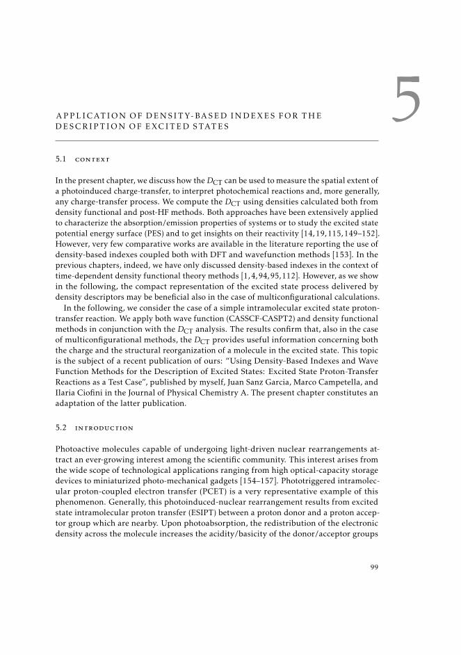
5APPL ICAT ION OF DENS ITY-BASED INDEXES FOR THE
DESCR IPT ION OF EXC ITED STATES
5.1 context
In the present chapter, we discuss how theDCT can be used to measure the spatial extent ofa photoinduced charge-transfer, to interpret photochemical reactions and, more generally,any charge-transfer process. We compute the DCT using densities calculated both fromdensity functional and post-HF methods. Both approaches have been extensively appliedto characterize the absorption/emission properties of systems or to study the excited statepotential energy surface (PES) and to get insights on their reactivity [14, 19, 115, 149–152].However, very few comparative works are available in the literature reporting the use ofdensity-based indexes coupled both with DFT and wavefunction methods [153]. In theprevious chapters, indeed, we have only discussed density-based indexes in the context oftime-dependent density functional theory methods [1,4,94,95,112]. However, as we showin the following, the compact representation of the excited state process delivered bydensity descriptors may be beneficial also in the case of multiconfigurational calculations.
In the following, we consider the case of a simple intramolecular excited state proton-transfer reaction. We apply both wave function (CASSCF-CASPT2) and density functionalmethods in conjunction with the DCT analysis. The results confirm that, also in the caseof multiconfigurational methods, the DCT provides useful information concerning boththe charge and the structural reorganization of a molecule in the excited state. This topicis the subject of a recent publication of ours: “Using Density-Based Indexes and WaveFunction Methods for the Description of Excited States: Excited State Proton-TransferReactions as a Test Case”, published by myself, Juan Sanz Garcia, Marco Campetella, andIlaria Ciofini in the Journal of Physical Chemistry A. The present chapter constitutes anadaptation of the latter publication.
5.2 introduction
Photoactive molecules capable of undergoing light-driven nuclear rearrangements at-tract an ever-growing interest among the scientific community. This interest arises fromthe wide scope of technological applications ranging from high optical-capacity storagedevices to miniaturized photo-mechanical gadgets [154–157]. Phototriggered intramolec-ular proton-coupled electron transfer (PCET) is a very representative example of thisphenomenon. Generally, this photoinduced-nuclear rearrangement results from excitedstate intramolecular proton transfer (ESIPT) between a proton donor and a proton accep-tor group which are nearby. Upon photoabsorption, the redistribution of the electronicdensity across the molecule increases the acidity/basicity of the donor/acceptor groups
99
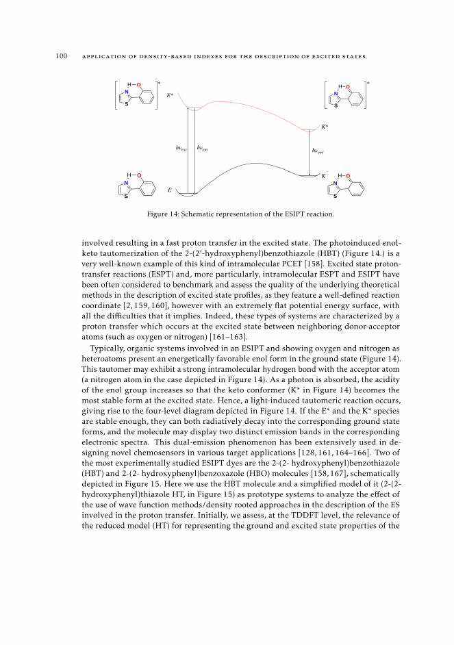
100 application of density-based indexes for the description of excited states
hνexc hνem hνem′
E
E*
K*
KN
S
H O
N
S
H O *
N
S
H O
N
S
H O *
Figure 14: Schematic representation of the ESIPT reaction.
involved resulting in a fast proton transfer in the excited state. The photoinduced enol-keto tautomerization of the 2-(2’-hydroxyphenyl)benzothiazole (HBT) (Figure 14.) is avery well-known example of this kind of intramolecular PCET [158]. Excited state proton-transfer reactions (ESPT) and, more particularly, intramolecular ESPT and ESIPT havebeen often considered to benchmark and assess the quality of the underlying theoreticalmethods in the description of excited state profiles, as they feature a well-defined reactioncoordinate [2, 159, 160], however with an extremely flat potential energy surface, withall the difficulties that it implies. Indeed, these types of systems are characterized by aproton transfer which occurs at the excited state between neighboring donor-acceptoratoms (such as oxygen or nitrogen) [161–163].
Typically, organic systems involved in an ESIPT and showing oxygen and nitrogen asheteroatoms present an energetically favorable enol form in the ground state (Figure 14).This tautomer may exhibit a strong intramolecular hydrogen bond with the acceptor atom(a nitrogen atom in the case depicted in Figure 14). As a photon is absorbed, the acidityof the enol group increases so that the keto conformer (K* in Figure 14) becomes themost stable form at the excited state. Hence, a light-induced tautomeric reaction occurs,giving rise to the four-level diagram depicted in Figure 14. If the E* and the K* speciesare stable enough, they can both radiatively decay into the corresponding ground stateforms, and the molecule may display two distinct emission bands in the correspondingelectronic spectra. This dual-emission phenomenon has been extensively used in de-signing novel chemosensors in various target applications [128, 161, 164–166]. Two ofthe most experimentally studied ESIPT dyes are the 2-(2- hydroxyphenyl)benzothiazole(HBT) and 2-(2- hydroxyphenyl)benzoxazole (HBO) molecules [158, 167], schematicallydepicted in Figure 15. Here we use the HBT molecule and a simplified model of it (2-(2-hydroxyphenyl)thiazole HT, in Figure 15) as prototype systems to analyze the effect ofthe use of wave function methods/density rooted approaches in the description of the ESinvolved in the proton transfer. Initially, we assess, at the TDDFT level, the relevance ofthe reduced model (HT) for representing the ground and excited state properties of the
5.3 computational details 101
N
S
H ON
S
H ON
O
H O
HBO HBT HT
Figure 15: Prototype molecules which can undergo ESIPT.
full HBT molecule, both in terms of energetic and of the charge-transfer (CT) character -evaluated through the DCT index [1,4]. Next, we analyze the excited state potential energysurface and the electronic properties of the HT molecule both at TDDFT and CASSCF-CASPT2 levels. Such calculations become possible thanks to the reduced dimension of theHT molecule which allows the use of reduced active space of 14 electrons in 12 orbitals,rather than 18 electrons in 16 orbitals (18e,16o) for the HBT molecule.
Here we examine the energetics and the CT profile of the reaction as calculated usingboth approaches. Our purpose is thus to assess if the relationship between the energeticfeatures of the reaction and theDCT profiles - previously defined in the context of TDDFT -still holds when multiconfigurational methods are employed. The discussion is structuredas follows: after a brief presentation of the computational details, we discuss the resultsobtained at the TDDFT level for the HBT molecule and the HT model. Next, we comparethe energetics (ES-PES) and the CT profiles (DCT index) computed for the HT model bothat the TDDFT and post-HF level, by scanning the PES along the two relevant, reactioncoordinates. Finally, we draw some general conclusions.
5.3 computational details
The ground-state potential energy surfaces (PES) of HBT and HT have been evaluatedperforming a two-dimensional (2D) relaxed scan. We have constructed a 2D grid byoptimizing one hundred homogeneously distributed structures, obtained by varyingindependently two constrained degrees of freedom: the N-O and O-H distances. Inparticular, we generated the structures varying the N-O distance from 2.54 to 2.72 Å inincrements of 0.02 Å, and the O-H distance from 0.99 to 1.89 Å in increments of 0.10Å to encompass the formulation of both the enol- and the keto-optimized forms. Onthe same grid, we computed the DCT index. With the idea of comparing densities andenergetics obtained by different methodologies, we calculated the GS relaxed scan atHartree-Fock, density functional theory (DFT), and complete active space self-consistentfield (CASSCF) [168] levels. On top of these, we computed excited state propertiesvertically using configuration interaction singles (CIS) [144], TDDFT [32], and completeactive space with second-order perturbation theory (CASPT2) [169] calculations. A forthe DFT and TDDFT calculations we used two different functionals: (i) the global hybridfunctional PBE0 [46] and (ii) the range separated asymptotically corrected LC-PBE [41,43]).Furthermore, we employed the same computational protocol to perform a relaxed scan of
102 application of density-based indexes for the description of excited states
the ES at CIS and TDDFT level. The wave function (WF) used in the CASPT2 calculationswas computed using the state-average-CASSCF (SA-CASSCF) technique with four equallyweighted roots (the ground state and three more excited states) and an active spaceconsisting on 14 electrons in 12 π orbitals delocalized in the whole planar HT molecule.Although CASSCF calculations are not able to recover dynamic correlation unless aprohibitively large active space is chosen, optimizations performed at the CASSCF levelwere the only feasible alternative to compute the optimized geometry grid. The evaluationof all optimized geometry energies at the GS (and ES) as well as vertical excitation energiesin the Franck-Condon (FC) region was performed at the SA-CASSCF(14,12)/CASPT2 levelof theory. We employed the imaginary shift technique (0.2 a.u.) to avoid the possiblepresence of intruder states [170], as previously reported in the literature for a similarorganic chromophore as described in Ref. [163].
All calculations were carried out using the same diffuse-augmented polarization valence-double-ζ basis set (6-31+G-(d)) [171] with one set of d polarization functions [172, 173]and a set of s and p diffuse functions [174, 175] for all atoms but hydrogens. All cal-culations, but the post-HF-based ones, were performed with the Gaussian 16 quantumpackage [145]. CASSCF, as well as CASPT2 calculations, were performed using theMOLCAS 8.0 quantum package [176]. No solvents effects were included.
As previously discussed in 4, the DCT density-based index allows to quantify the spatialextent of a charge-transfer excitation simply and intuitively. Using the electronic densitiesof the ground and excited state of interest (here the first singlet), ρGS(r) and ρEX(r),respectively, the DCT has been mapped on the optimized GS and ES grid. For TDDFTcalculations, the DCT index was directly computed using the Gaussian 16 program [145],using both relaxed and unrelaxed densities. For the CASPT2 calculations, on the otherhand, we computed the DCT from the real space ground and excited state densities, usinga freely distributed software of ours [177].
5.4 assessment of the model system: ht vs hbt
To validate the use of the HT system (Figure 14) as a reasonable model to describe theESIPT reaction of HBT, we performed TDDFT calculations using different functionals forboth systems. Energy and DCT maps were computed for both systems, as described inthe previous section. In particular, ground state PESs were constructed, for both HT andHBT, performing a relaxed scan over the N-O and O-H coordinates, computed at the PBE0level of theory, followed by single-point TDDFT calculations performed using the PBE0and LC-PBE functional as well as at CIS level. Excited state parameters were obtainedvertically from the optimized ground state geometries, using the same approach.
All systems obtained show a planar structure. Table 5 collects the energetic parametersmost relevant to describe the enol to keto tautomerization, as extracted from the computed2D maps. At the GS, the enol tautomer is the most stable in the PES (all values relative toHBT are in parentheses in the following), while the keto form appears at higher energyvalues, both for the HT and HBT molecule, independently of the method considered.Although the keto-enol energy difference is dependent on the method used, for a given
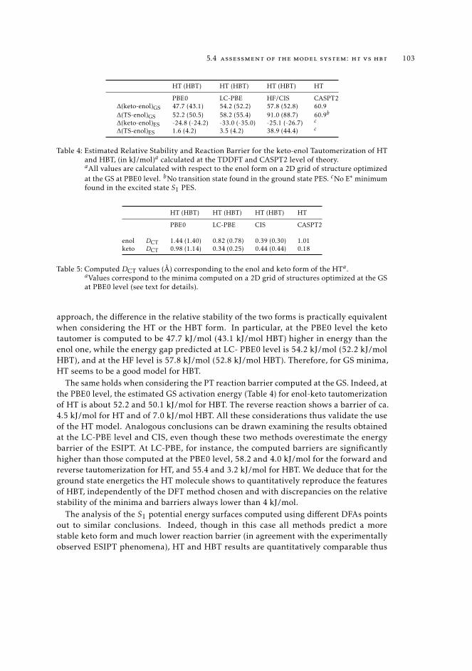
5.4 assessment of the model system: ht vs hbt 103
HT (HBT) HT (HBT) HT (HBT) HT
PBE0 LC-PBE HF/CIS CASPT2∆(keto-enol)GS 47.7 (43.1) 54.2 (52.2) 57.8 (52.8) 60.9∆(TS-enol)GS 52.2 (50.5) 58.2 (55.4) 91.0 (88.7) 60.9b
∆(keto-enol)ES -24.8 (-24.2) -33.0 (-35.0) -25.1 (-26.7) c
∆(TS-enol)ES 1.6 (4.2) 3.5 (4.2) 38.9 (44.4) c
Table 4: Estimated Relative Stability and Reaction Barrier for the keto-enol Tautomerization of HTand HBT, (in kJ/mol)a calculated at the TDDFT and CASPT2 level of theory.aAll values are calculated with respect to the enol form on a 2D grid of structure optimizedat the GS at PBE0 level. bNo transition state found in the ground state PES. cNo E∗ minimumfound in the excited state S1 PES.
HT (HBT) HT (HBT) HT (HBT) HT
PBE0 LC-PBE CIS CASPT2
enol DCT 1.44 (1.40) 0.82 (0.78) 0.39 (0.30) 1.01keto DCT 0.98 (1.14) 0.34 (0.25) 0.44 (0.44) 0.18
Table 5: Computed DCT values (Å) corresponding to the enol and keto form of the HTa.aValues correspond to the minima computed on a 2D grid of structures optimized at the GSat PBE0 level (see text for details).
approach, the difference in the relative stability of the two forms is practically equivalentwhen considering the HT or the HBT form. In particular, at the PBE0 level the ketotautomer is computed to be 47.7 kJ/mol (43.1 kJ/mol HBT) higher in energy than theenol one, while the energy gap predicted at LC- PBE0 level is 54.2 kJ/mol (52.2 kJ/molHBT), and at the HF level is 57.8 kJ/mol (52.8 kJ/mol HBT). Therefore, for GS minima,HT seems to be a good model for HBT.
The same holds when considering the PT reaction barrier computed at the GS. Indeed, atthe PBE0 level, the estimated GS activation energy (Table 4) for enol-keto tautomerizationof HT is about 52.2 and 50.1 kJ/mol for HBT. The reverse reaction shows a barrier of ca.4.5 kJ/mol for HT and of 7.0 kJ/mol HBT. All these considerations thus validate the useof the HT model. Analogous conclusions can be drawn examining the results obtainedat the LC-PBE level and CIS, even though these two methods overestimate the energybarrier of the ESIPT. At LC-PBE, for instance, the computed barriers are significantlyhigher than those computed at the PBE0 level, 58.2 and 4.0 kJ/mol for the forward andreverse tautomerization for HT, and 55.4 and 3.2 kJ/mol for HBT. We deduce that for theground state energetics the HT molecule shows to quantitatively reproduce the featuresof HBT, independently of the DFT method chosen and with discrepancies on the relativestability of the minima and barriers always lower than 4 kJ/mol.
The analysis of the S1 potential energy surfaces computed using different DFAs pointsout to similar conclusions. Indeed, though in this case all methods predict a morestable keto form and much lower reaction barrier (in agreement with the experimentallyobserved ESIPT phenomena), HT and HBT results are quantitatively comparable thus
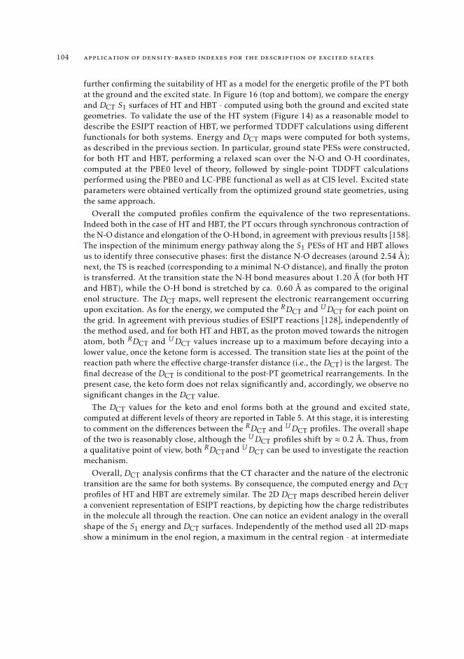
104 application of density-based indexes for the description of excited states
further confirming the suitability of HT as a model for the energetic profile of the PT bothat the ground and the excited state. In Figure 16 (top and bottom), we compare the energyand DCT S1 surfaces of HT and HBT - computed using both the ground and excited stategeometries. To validate the use of the HT system (Figure 14) as a reasonable model todescribe the ESIPT reaction of HBT, we performed TDDFT calculations using differentfunctionals for both systems. Energy and DCT maps were computed for both systems,as described in the previous section. In particular, ground state PESs were constructed,for both HT and HBT, performing a relaxed scan over the N-O and O-H coordinates,computed at the PBE0 level of theory, followed by single-point TDDFT calculationsperformed using the PBE0 and LC-PBE functional as well as at CIS level. Excited stateparameters were obtained vertically from the optimized ground state geometries, usingthe same approach.
Overall the computed profiles confirm the equivalence of the two representations.Indeed both in the case of HT and HBT, the PT occurs through synchronous contraction ofthe N-O distance and elongation of the O-H bond, in agreement with previous results [158].The inspection of the minimum energy pathway along the S1 PESs of HT and HBT allowsus to identify three consecutive phases: first the distance N-O decreases (around 2.54 Å);next, the TS is reached (corresponding to a minimal N-O distance), and finally the protonis transferred. At the transition state the N-H bond measures about 1.20 Å (for both HTand HBT), while the O-H bond is stretched by ca. 0.60 Å as compared to the originalenol structure. The DCT maps, well represent the electronic rearrangement occurringupon excitation. As for the energy, we computed the RDCT and UDCT for each point onthe grid. In agreement with previous studies of ESIPT reactions [128], independently ofthe method used, and for both HT and HBT, as the proton moved towards the nitrogenatom, both RDCT and UDCT values increase up to a maximum before decaying into alower value, once the ketone form is accessed. The transition state lies at the point of thereaction path where the effective charge-transfer distance (i.e., the DCT) is the largest. Thefinal decrease of the DCT is conditional to the post-PT geometrical rearrangements. In thepresent case, the keto form does not relax significantly and, accordingly, we observe nosignificant changes in the DCT value.
The DCT values for the keto and enol forms both at the ground and excited state,computed at different levels of theory are reported in Table 5. At this stage, it is interestingto comment on the differences between the RDCT and UDCT profiles. The overall shapeof the two is reasonably close, although the UDCT profiles shift by ≈ 0.2 Å. Thus, froma qualitative point of view, both RDCTand UDCT can be used to investigate the reactionmechanism.
Overall, DCT analysis confirms that the CT character and the nature of the electronictransition are the same for both systems. By consequence, the computed energy and DCTprofiles of HT and HBT are extremely similar. The 2D DCT maps described herein delivera convenient representation of ESIPT reactions, by depicting how the charge redistributesin the molecule all through the reaction. One can notice an evident analogy in the overallshape of the S1 energy and DCT surfaces. Independently of the method used all 2D-mapsshow a minimum in the enol region, a maximum in the central region - at intermediate
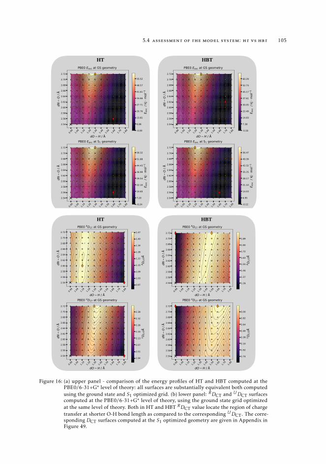
5.4 assessment of the model system: ht vs hbt 105
HT HBT
HT HBT
Figure 16: (a) upper panel - comparison of the energy profiles of HT and HBT computed at thePBE0/6-31+G* level of theory: all surfaces are substantially equivalent both computedusing the ground state and S1 optimized grid. (b) lower panel: RDCT and UDCT surfacescomputed at the PBE0/6-31+G* level of theory, using the ground state grid optimizedat the same level of theory. Both in HT and HBT RDCT value locate the region of chargetransfer at shorter O-H bond length as compared to the corresponding UDCT. The corre-sponding DCT surfaces computed at the S1 optimized geometry are given in Appendix inFigure 49.
106 application of density-based indexes for the description of excited states
N-O and O-H distances, and fall into a minimum as the proton moves toward the nitrogen.This evidence suggests that the DCT could be used just as the energy to locating minima,and transition states on the excited state potential energy surfaces.
Finally, we computed all ground-state optimized geometries at the PBE0 level. Accord-ingly, we computed excited states vertically on top of this geometries - using LC-PBE andCIS. For the sake of completeness and to check that no artifact was introduced in such away, we optimized the ground states and computed the corresponding vertical excitedstate surfaces, at each level of theory. All different methods result in nearly identicalgeometries, and no significant change was found in the two-dimensional contour maps(see Appendix 49). Hence, independently of the level of theory used, HT and HBT resultnearly identical. These pieces of evidence ultimately validate the use of HT as a modelsystem to elucidate quantitatively ESPT phenomena occurring in the HBT molecule. Thus,in the following, we limit the discussion to HT only.
5.5 description of the esipt in ht using casscf-caspt2 calculations and
density based indexes.
At this point, we remind that neither the ground and first excited state PESs nor the firstand second excited state surfaces of HT cross each other when the molecule is kept planar(as in the present case). This observation holds both in TDDFT and CASPT2. Accordingly,within the PES region studied, where the molecule is strictly planar, the electronic natureof the first singlet excited state remains unvaried (ππ∗ state). We therefore limit thediscussion to the first excited state. We proceed to examine the same reaction using thedensity computed from multireference post-HF methods. For this purpose, we computedthe ESIPT in HT at CASSCF-CASPT2 level and analyzed the energy and DCT profiles onthe same grid as previously done for TDDFT computed surfaces.
Let us first illustrate the topology of the ES PES and the corresponding DCT mapcomputed at the CASPT2 level, focusing on the Franck- Condon region. Based on CASPT2calculations and in agreement with DFT results, at the ground state, the HT moleculeexclusively exists in the enol tautomer form as confirmed by the higher energy stabilityof the enol relative to the keto form (60.9 kJ/ mol, Table 4). The redistribution of theelectronic density across the molecule results that occurs upon absorption results in theincreased acidity of the oxygen and basicity of the nitrogen, leading to the excited statetautomerization. The aromatic rings contribute to stabilize and promote the CT process,as confirmed by the difference between the sums of CASPT2 Mulliken charges. The phenolmoiety, which has a total charge of (0.31 |e-|) in the ground state increases its charge atthe excited state (0.44 |e-|). Correspondingly the overall charge in the thiazole fragmentdecreases from (-0.31 |e-|) to-0.44 |e-|).
Nonetheless, due to the arbitrary nature of the partition scheme used to compute atomiccharges, it is hard to assess quantitatively the magnitude of the CT based on the soleanalysis of atomic charges. Such imprecision can be avoided applying aDCT based analysiswhich provides a neat solution to this ambiguity. This index allows both to quantify thespatial extent of the CT excitation and contextually to define the donor/acceptor molecular
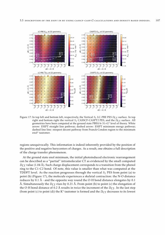
5.5 description of the esipt in ht using casscf-caspt2 calculations and density based indexes. 107
E*K* E* K*
b)b)b)
a)
b) c) d)
E*K*
E* K*
Figure 17: In top left and bottom left, respectively, the Vertical S1 LC-PBE PES DCT surface. In topright and bottom right the vertical S1 CASSCF-CASPT2 PES, and the DCT surface. Allgeometries have been computed at the ground state PBE0/6-31+G* level of theory. Whitearrow: ESIPT straight line pathway; dashed arrow: ESIPT minimum energy pathway;dashed line line: steepest decent pathway from Franck-Condon region to the minimumenol* tautomer.
regions unequivocally. This information is indeed inherently provided by the position ofthe positive and negative barycenters of charges. As a result, one obtains a full descriptionof the charge transfer phenomenon.
At the ground state enol minimum, the initial photoinduced electronic rearrangementcan be described as a “partial” intramolecular CT as evidenced by the small computedDCT value (1.04 Å). Such charge displacement corresponds to a transition from the phenolring to the C1-C2 bond. Of note, this value is smaller than what was computed at theTDDFT level. As the reaction progresses through the vertical S1 PES from point (a) topoint (b) (Figure 17), the molecule experiences a skeletal contraction: the N-O distancereduces by 0.1 Å - and the opposite way round the O-H bond distance elongates by 0.1Å. Simultaneously the DCT rises by 0.21 Å. From point (b) to point (c) the elongation ofthe O-H bond distance of 0.2 Å results in twice the increment of the DCT. In the last step(from point (c) to point (d)) the K* tautomer is formed and the DCT decreases to its lowest
108 application of density-based indexes for the description of excited states
value - the O-H bond distance increases by an additional 0.4 Å. The direct comparisonof the topological features between S1 PES and DCT surface reveals remarkable commonpatterns independently of the method used. For instance, in the case of LC-PBE (see thetop of Figure 17) both surfaces present a flat E* minimum, while a steep well-definedminimum appears in the K* region. In both surfaces (S1 and DCT) a hill separates the enoland keto region. Similar features also appear in the CIS profiles, though unlike in the DFTsurfaces, the E* minimum is much steeper both in the S1 PES and in the DCT surfaces - alladditional figures not shown in the main text can be found in Appendix, in Section 11.2.
Thus, the parallelism between energy and DCT index remains valid also in this case:DCT and energy surface have matching behavior. By contrast, unlike the PBE0, LC-PBE,and CIS vertical S1 PESs, the CASPT2 surface does not show any E* minima but onlya steep downhill slope at the Franck-Condon region which points toward the global K*minimum, with no other local minima along the steepest descent trajectory. This barrier-less adiabatic S1 pathway though is in agreement with previous findings [128] on ESIPTreactions studied at CASSCF-CASPT2 level.
As previously alluded to, optimizing the GS geometries at different levels of theoryaffords nearly identical structures. This results in the S1 PES and DCT surfaces beingqualitatively the same with no remarkable differences to those computed using the PBE0ground state optimized grid. By contrast, the relaxed (optimized) S1 surfaces are visiblydifferent as computed with each method. The only meaningful S1 relaxed surfaces are theone computed using the relaxed S1 PBE0 geometries (in Figure 49). Regarding the gridvalues computed using the optimized S1 structures, we observe, as a general trend thatthe minima in the excited state PES become steeper and more localized as compared tothose observed in the vertical 2D grids, obtained using the GS geometries. This behavioris even more pronounced in the DCT surfaces (see Appendix 49).
5.6 conclusions
Using a prototype excited state proton-transfer reaction as a test case we have shown thatdensity-based descriptors (such as the DCT index) can be safely used to analyze excitedstates qualitatively and quantitatively, both at the TDDFT and post-HF level of theory(here CASSCF- CASPT2). Our study shows that the DCT provides a good descriptionof the electronic rearrangements during a photochemical reaction and delivers relevantinformation about the structure of the molecule, suggesting that the DCT could be usedto locate minima on a PES. This particular feature makes the DCT a perfect candidatefor optimization of stationary structures in excited states. Besides, the DCT can be ofparticular relevance to quantify CT in complex systems avoiding arbitrary evaluationbased on charge partitioning.
For the first time, we have examined a reaction using a multiconfigurational wave-function method coupled with the DCT. Our investigation confirms that any electronicstructure method can be coupled to density-based indexed, as long as it provides accurateelectronic densities for the ground and excited states, having a physical meaning in anyregion of a PES. Of course, all limitations concerning the DCT itself (for instance its

5.6 conclusions 109
null value by construction in the case of systems with quadrupole-like symmetry) holdindependently of the underlying electronic method used to access to ground and excitedstate densities. In such cases, one may partition the molecule in asymmetric units andcompute the DCT separately on each fragment, as suggested in reference [118].

6THE PROBLEMAT IC DESCR IPT ION OF CHARGE -TRANSFER
EXC ITAT IONS US ING DFT
6.1 context
When TDDFT is used, through-space charge-transfer (CT) states happen to correspondto excited states in which photoexcited hole and electron charge distributions poorlyoverlap. This outcome, however, is typically an artifact of the method resulting from theuse of approximate xc-potentials, which have incorrect functional asymptotics and areerroneously continuous. As discussed in Section 2.4.5, the exact exchange-correlationpotential of a charge-transfer state jumps discontinuously by an amount ∆xc as the numberof electrons crosses the integer. As a consequence, the excitation energies for such statesare usually significantly underestimated to the point that they can appear below theoptical states. In the present chapter we discuss a methodology to spot these spuriousunphysical states, through a new and computationally inexpensive index - MAC.
The formulation of the MAC index is derived as a modification of the Mulliken estima-tion of transition energy for CT excitations. It relies on two basic ingredients: an effectiveCT distance, computed using our density-based index (DCT), and an orbital weightedestimation of the ionization potential and electron affinity. To verify the robustness ofour approach we have tested our index on some model systems, representative of bothintermolecular and intramolecular CT excitations by utilizing functionals belonging todifferent classes (generalized gradient approximation, global hybrids and range separatedhybrids). These preliminary results confirm that ghost states are correctly spotted, alsoin the delicate case of intramolecular excitations displaying substantial donor-bridge-acceptor delocalization, regime in which the standard Mulliken formulation attends itslimits. This first part of the chapter is adapted from a previous publication of myself,Marco Campetella, Mike J. Frisch, Giovanni Scalmani, Ilaria Ciofini and Carlo Adamo [5].
Furthermore, we have applied the MAC index to the several organic dyes. Such analysisfits within the broader context of the construction of a comprehensive strategy for thedescription of photochemical processes, based on density-based indexes. Here we examinethe charge-transfer excitations of different molecules evolving along a reaction coordinate,so to verify the correctness and reliability of the potential energy curves that we laterexamine with the aim to monitor the evolution of the excited states along the samecoordinate - as discussed in the Chapter 8.
6.2 introduction
TDDFT represents a sophisticated, yet moderately expensive tool to calculate excited statesproperties for a large variety of molecules in the gas-phase, in solution or even in more
111
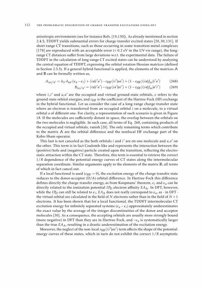
112 the problematic description of charge-transfer excitations using dft
anisotropic environments (see for instance Refs. [19,130]). As already mentioned in section2.4.5, TDDFT yields substantial errors for charge-transfer excited states [20, 30,131]. Ifshort-range CT transitions, such as those occurring in some transition metal complexes[178] are reproduced with an acceptable error (< 0.2 eV in the UV-vis range), the long-range CT distances suffer from large deviations w.r.t. the experimental data. The failure ofTDDFT in the calculation of long-range CT excited states can be understood by analyzingthe central equation of TDDFT, expressing the orbital rotation Hessian matrices (definedin Section 2.5.5). If a general hybrid functional is applied, the elements of the matrices A
and B can be formally written as,
Aia,i′a′ = δii′δaa′ (εa − εi) + (ia|i′a′)− cHF(ii′ |aa′) + (1− cHF)(ia|fxc|i′a′) (268)
Bia,i′a′ = (ia|i′a′)− cHF(ia′ |ai′) + (1− cHF)(ia|fxc|a′i′) (269)
where i, i′ and a,a′ are the occupied and virtual ground-state orbitals, ε refers to theground-state orbital energies, and cHF is the coefficient of the Hartree-Fock (HF) exchangein the hybrid functional. Let us consider the case of a long-range charge-transfer statewhere an electron is transferred from an occupied orbital i on a molecule, to a virtualorbital a of different one. For clarity, a representation of such scenario is given in Figure18. If the molecules are sufficiently distant in space, the overlap between the orbitals onthe two molecules is negligible. In such case, all terms of Eq. 268, containing products ofthe occupied and virtual orbitals, vanish [20]. The only remaining terms which contributeto the matrix A are the orbital difference and the nonlocal HF exchange part of theKohn-Sham operator.
This last is not canceled as the both orbitals i and i′ are on one molecule and a,a′ onthe other. This term is in fact Coulomb-like and represents the interaction between the(positive) hole and (negative) particle created upon the transition, reflecting the electro-static attraction within the CT state. Therefore, this term is essential to retrieve the correct1/R dependence of the potential energy curves of CT states along the intermolecularseparation coordinate. Similar arguments apply to the elements of the matrix B, all termsof which in fact cancel out.
If a local functional is used (cHF = 0), the excitation energy of the charge-transfer statereduces to the donor-acceptor (D/A) orbital difference. In Hartree-Fock this differencedefines directly the charge-transfer energy, as from Koopmans’ theorem, εi and εa can bedirectly related to the ionization potential IPD electron affinity EAA. In DFT, however,while the IPD can still be related to εi , EAA does not really correspond to εa, as - in DFT -the virtual orbital are calculated in the field of N electrons rather than in the field of N+1electrons. It has been shown that for a local functional, the TDDFT intermolecular CTexcitation energy for infinitely separated systems (εa − εi ) approximately underestimatesthe exact value by the average of the integer discontinuities of the donor and acceptormolecules [30]. As a consequence, the accepting orbitals are usually more strongly bound(more negative) in DFT than they are in Hartree-Fock, and −εa is systematically largerthan the true EAA, resulting in a drastic underestimation of the excitation energy.
Moreover, the neglect of the non-local cHF(ii′ |aa′) term affects the shape of the potential-
energy curves of these states, which in turn do not exhibit the correct 1/R asymptotic
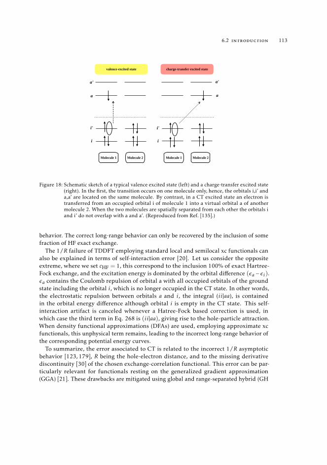
6.2 introduction 113
Molecule 1 Molecule 2
valence-excited state charge-transfer excited state
Molecule 1 Molecule 2
i
i'
a
a'
i
i'
a
a'
Figure 18: Schematic sketch of a typical valence excited state (left) and a charge-transfer excited state(right). In the first, the transition occurs on one molecule only, hence, the orbitals i,i’ anda,a’ are located on the same molecule. By contrast, in a CT excited state an electron istransferred from an occupied orbital i of molecule 1 into a virtual orbital a of anothermolecule 2. When the two molecules are spatially separated from each other the orbitals iand i’ do not overlap with a and a’. (Reproduced from Ref. [135].)
behavior. The correct long-range behavior can only be recovered by the inclusion of somefraction of HF exact exchange.
The 1/R failure of TDDFT employing standard local and semilocal xc functionals canalso be explained in terms of self-interaction error [20]. Let us consider the oppositeextreme, where we set cHF = 1, this correspond to the inclusion 100% of exact Hartree-Fock exchange, and the excitation energy is dominated by the orbital difference (εa − εi).εa contains the Coulomb repulsion of orbital a with all occupied orbitals of the groundstate including the orbital i, which is no longer occupied in the CT state. In other words,the electrostatic repulsion between orbitals a and i, the integral (ii|aa), is containedin the orbital energy difference although orbital i is empty in the CT state. This self-interaction artifact is canceled whenever a Hatree-Fock based correction is used, inwhich case the third term in Eq. 268 is (ii|aa), giving rise to the hole-particle attraction.When density functional approximations (DFAs) are used, employing approximate xcfunctionals, this unphysical term remains, leading to the incorrect long-range behavior ofthe corresponding potential energy curves.
To summarize, the error associated to CT is related to the incorrect 1/R asymptoticbehavior [123, 179], R being the hole-electron distance, and to the missing derivativediscontinuity [30] of the chosen exchange-correlation functional. This error can be par-ticularly relevant for functionals resting on the generalized gradient approximation(GGA) [21]. These drawbacks are mitigated using global and range-separated hybrid (GH
114 the problematic description of charge-transfer excitations using dft
and RSH) functionals, which introduce, in a different way, a fraction of Hartree-Fock(HF)-like exchange [58]. Even better results can be obtained by less-standard and morecomputationally demanding methods, for instance, by tuning the RSH functional on thesystem under investigation [29]. Unfortunately, the excitation energies provided are oftenoverestimated by RSH and not always of sufficient quality to allow for a quantitativeagreement with the experimental spectra [180], so that most calculations still resort onthe use of GH which are those still potentially affected by error in the estimation of CTtransitions.
6.3 a ghost-hunter index for charge-transfer excitations
We have now recalled what is the charge-transfer problem and what does it originate.Charge-transfer excitations, play a key role in many systems of relevance for biologicaland/or technological application, such as, for instance, light-harvesting complexes inplants and bacteria or as semi-conductor polymers [181, 182]. Hence, the issue of CTexcitations in TDDFT has been largely debated in literature [129, 132, 183]), and severalsolutions have been suggested to diagnostic [184] and correct this failure [20,131]. Besidesan erroneous evaluation of electronic energies, which can be monitored by dedicateddiagnostic indexes [19, 103, 120, 121, 180], the energy underestimation of the charge-transfer virtual orbitals causes TDDFT to be affected by another major drawback: theappearance of low-lying CT ghost states energetically well below the bright (real) stateof a given system for both intermolecular and intramolecular excitations [131]. Thisspurious effect can be very important for the interpretation and prediction of the spec-troscopic properties of a given molecular system as it would suggest, for instance, thatan energetically higher bright state could decay non-radiatively into the lower CT states,leading to an electron-transfer quenching of the excited state fluorescence. In other words,the limitations of the TDDFT model used have an impact that is much larger than itsnumerical performances, (i.e., the error in computed transition energies w.r.t. a givenreference) leading to a wrong interpretation of the photophysical behavior of the systemunder investigation. The undesirable consequences for chemical applications of thesecomputational models are evident.
The existence of these low-lying CT states, referred to as “ghost” states, was discussedin the seminal works of Dreuw and Head-Gordon [131, 148]. In the case of a donor (D) –acceptor (A) system and assuming that the separated charges in the CT states could betreated as point charges, these authors showed that the distance-dependent excitationenergy of the energetically lowest CT state ωCT(R) can simply be estimated via
ωCT ≥ IPD −EAA − 1R
. (270)
where R is the distance between the two subsystems and IPD is the ionization potentialof the donor, EAA is the electron affinity of the acceptor, and 1/R is the electrostaticattraction between them. In this equation, the cation and anion are treated as pointcharges and the shortest possible distance R is assumed, which of course leads to an
6.3 a ghost-hunter index for charge-transfer excitations 115
overestimation of the electrostatic attraction. Previously, this simple and intuitive relation,has been used to verify the nature of TDDFT excitations in model systems [58, 131, 148],considering R as the geometrical distance between the donor and acceptor units andevaluating IP and EA from the Koopmans’ theorem (i.e., from HOMO and LUMO orbitalenergies).
In this context, with the aim of providing a simple and robust reliable tool for thedetection of ghost CT states in TDDFT, we have conceived a new descriptor, MAC, basedon a modification of - Eq. 270. MAC is the acronym for Mulliken averaged configuration asthe definition, retraces the discussion on charge-transfer excitations originally proposedby Mulliken [86].
Eq. 270 can be considered as a lower energetic bound for a true CT transition. However,it is evident that this guesstimate remains rather inaccurate, when DFAs are used, asnone of the terms is actually close to being exact. With little effort though, one can refineeach term of Eq. 270, so to obtain a more reliable estimate of the minimal energy for acharge-transfer excitation. This is the basic idea behind the MAC index, which is thusdefined as
MAC =∑ia
c2ia(|εa| − εi)∑ia c
2ia
− 1DCT
. (271)
Here the DCT - in the place of R in Eq. 270 - provides a refined measure of the hole-electron distance. As we mentioned previously in Chapter 4, the DCT is computed as thedistance between the two barycenters of the spatial regions corresponding to an increaseand to a decrease of the electron density upon excitation [1]. Therefore, it represents, in avery realistic and intuitive fashion, the effective (average) charge/hole distance associatedto an electronic excitation. As for the remaining terms, Eq. 270 is obviously constrainedto estimate the energy of the first and lowest CT transition, as it is defined from IPand EA, which, from Koopmans’ theorem we may approximate as the negative of thefrontier orbitals energy. One can virtually establish the minimal energetic bound ofany given charge-transfer transition by substituting the HOMO and LUMO with theorbitals pairs (εi ,εa) actually involved in the transition. As any electronic transition inTDDFT is more generally defined as a combination of different one-electron excitations,we replace IPD and EAA in Eq. 270 using a weighted average of the starting (εi ) and final(εa) Kohn–Sham orbital energies. The absolute value ensures that IP and EA - derivedfrom TDDFT - remain in the same relation as they appear in the original equation byMulliken, and retain their chemical meaning. The weights for IPD and EAA, cia are theCI coefficients obtained as solution of TDDFT equations [21].
The MAC index, defined in Eq. 271 defines the lowest threshold for a given transition,and can be used to diagnostic the presence of unphysical low-lying transitions. A givenTDDFT transition will be, therefore, identified as ghost (and discharged) if its energy islower than the corresponding MAC index, while proper CT excitations will have an energygreater than MAC. Thus, for each electronic transition
ETDDFT <MAC =⇒ ghost ct state (272)
ETDDFT >MAC =⇒ real ct state. (273)
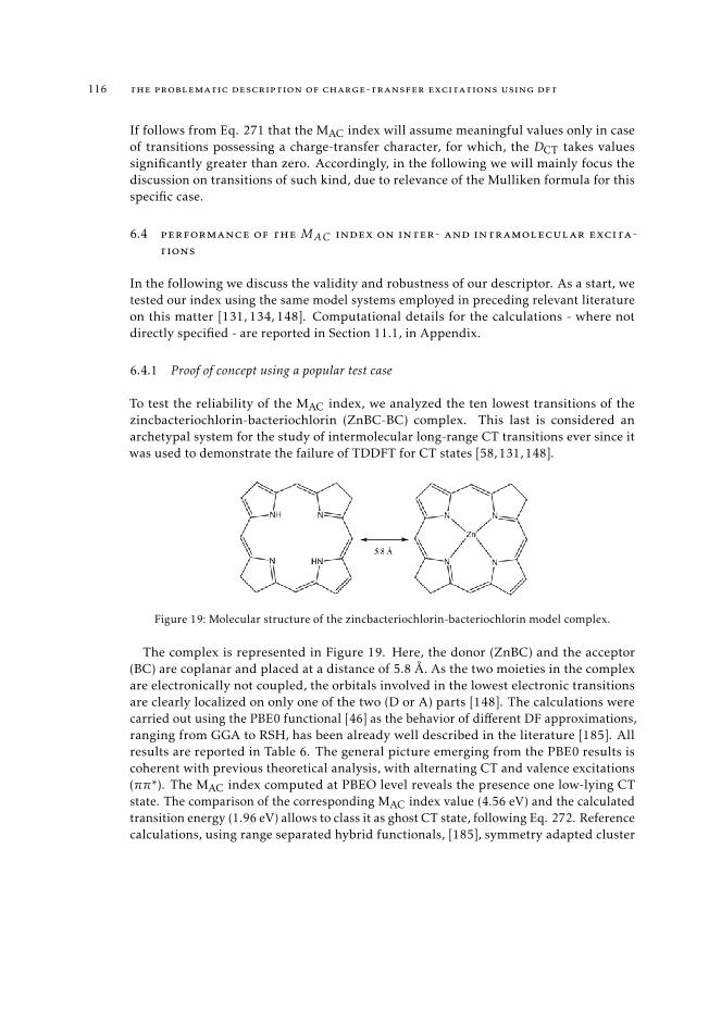
116 the problematic description of charge-transfer excitations using dft
If follows from Eq. 271 that the MAC index will assume meaningful values only in caseof transitions possessing a charge-transfer character, for which, the DCT takes valuessignificantly greater than zero. Accordingly, in the following we will mainly focus thediscussion on transitions of such kind, due to relevance of the Mulliken formula for thisspecific case.
6.4 performance of the MAC index on inter- and intramolecular excita-
tions
In the following we discuss the validity and robustness of our descriptor. As a start, wetested our index using the same model systems employed in preceding relevant literatureon this matter [131, 134, 148]. Computational details for the calculations - where notdirectly specified - are reported in Section 11.1, in Appendix.
6.4.1 Proof of concept using a popular test case
To test the reliability of the MAC index, we analyzed the ten lowest transitions of thezincbacteriochlorin-bacteriochlorin (ZnBC-BC) complex. This last is considered anarchetypal system for the study of intermolecular long-range CT transitions ever since itwas used to demonstrate the failure of TDDFT for CT states [58, 131, 148].
Figure 19: Molecular structure of the zincbacteriochlorin-bacteriochlorin model complex.
The complex is represented in Figure 19. Here, the donor (ZnBC) and the acceptor(BC) are coplanar and placed at a distance of 5.8 Å. As the two moieties in the complexare electronically not coupled, the orbitals involved in the lowest electronic transitionsare clearly localized on only one of the two (D or A) parts [148]. The calculations werecarried out using the PBE0 functional [46] as the behavior of different DF approximations,ranging from GGA to RSH, has been already well described in the literature [185]. Allresults are reported in Table 6. The general picture emerging from the PBE0 results iscoherent with previous theoretical analysis, with alternating CT and valence excitations(ππ*). The MAC index computed at PBEO level reveals the presence one low-lying CTstate. The comparison of the corresponding MAC index value (4.56 eV) and the calculatedtransition energy (1.96 eV) allows to class it as ghost CT state, following Eq. 272. Referencecalculations, using range separated hybrid functionals, [185], symmetry adapted cluster
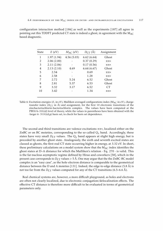
6.4 performance of the MAC index on inter- and intramolecular excitations 117
configuration interaction method [186] as well as the experiments [187] all agree inpointing out this TDDFT predicted CT state is indeed a ghost, in agreement with the MACbased diagnostic.
State E (eV) MAC (eV) DCT (Å) Assignment
1 1.97 (1.94) 4.56 (5.03) 6.62 (6.64) Ghost2 2.06 (2.00) - 0.37 (0.29) ππ∗3 2.11 (2.06) - 0.17 (0.56) ππ∗4 2.13 (2.10) 4.69 6.64 (6.67) Ghost5 2.54 - 0.69 ππ∗6 2.58 - 1.28 ππ∗7 2.72 5.24 6.52 Ghost8 2.81 5.37 6.53 Ghost9 3.32 3.17 6.52 CT
10 3.42 - 1.34 ππ∗
Table 6: Excitation energies (E, in eV), Mulliken averaged configurations index (MAC in eV), charge-transfer index (DCT in Å) and assignment, for the first 10 electronic transitions of thezincbacteriochlorin-bacteriochlorin complex. The values have been computed at thePBE0/6–31G(d) level of theory, while the values in parentheses have been obtained with the-larger 6- 311G(d,p) basis set, to check for basis set dependence.
The second and third transitions are valence excitations ππ∗, localized either on theZnBC or on BC moieties, corresponding to the so-called Qx band. Accordingly, thesestates have very small DCT values. The Qy band appears at slight high energy, but ispreceded by another ghost state. Analogously, the sixth and seventh excited states areclassed as ghosts, the first real CT state occurring higher in energy, at 3.32 eV. In short,these preliminary calculations on a model system show that the MAC index identifies theghost states at D–A distance for which the Mulliken’s relation - Eq. 270 - is valid. Thisis the far-nucleus asymptotic regime defined by Hirao and coworkers [58], which in thepresent case corresponds toDCT values > 5 Å. One may argue that the the ZnBC-BC modelcomplex is an "easy case", as the hole-electron distance is comparable to the geometricaldistance between the D and A moieties [131]. Indeed, the edge-to-edge distance (5.8 Å) isnot too far from the DCT values computed for any of the CT transitions (6.5–6.6 Å).
Real chemical systems are, however, a more difficult playground, as holes and electronsare often not clearly localized, due to electronic conjugation/delocalization effects. Theeffective CT distance is therefore more difficult to be evaluated in terms of geometricalparameters only.
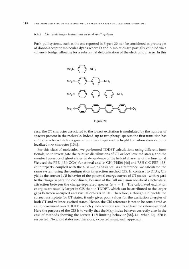
118 the problematic description of charge-transfer excitations using dft
6.4.2 Charge-transfer transitions in push-pull systems
Push-pull systems, such as the one reported in Figure 20, can be considered as prototypesof donor–acceptor molecular dyads where D and A moieties are partially coupled via a–phenyl- bridge, allowing for a substantial delocalization of the electronic charge. In this
Me2N NO2
Me2N
Me2N
Me2N
NO2
NO2
NO2
Figure 20
case, the CT character associated to the lowest excitation is modulated by the number ofspacers present in the molecule. Indeed, up to two phenyl spacers the first transition hasa CT character while for a greater number of spacers the bright transition shows a morelocalized ππ∗ character [134].
For this class of molecules, we performed TDDFT calculations using different func-tionals, so to investigate the relative distributions of CT or local excited states, and theeventual presence of ghost states, in dependence of the hybrid character of the functional.We used the PBE [43] (GGA) functional and its GH (PBE0) [46] and RSH (LC-PBE) [58]counterparts, coupled with the 6-31G(d,p) basis set. As a reference, we calculated thesame system using the configuration interaction method CIS. In contrast to DFAs, CISyields the correct 1/R behavior of the potential energy curves of CT states - with regardto the charge separation coordinate, because of the full inclusion non-local electrostaticattraction between the charge-separated species (cHF = 1). The calculated excitationenergies are usually larger in CIS than in TDDFT, which can be attributed to the largergaps between occupied and virtual orbitals in HF. Therefore, although CIS yields thecorrect asymptote for CT states, it only gives poor values for the excitation energies ofboth CT and valence-excited states. Hence, the CIS reference is not to be considered asan improvement over TDDFT - which yields accurate results at least for valence-excited.Here the purpose of the CIS is to verify that the MAC index behaves correctly also in thecase of methods showing the correct 1/R limiting behavior [58], i.e. when Eq. 270 isrespected. No ghost states are, therefore, expected using such approach.
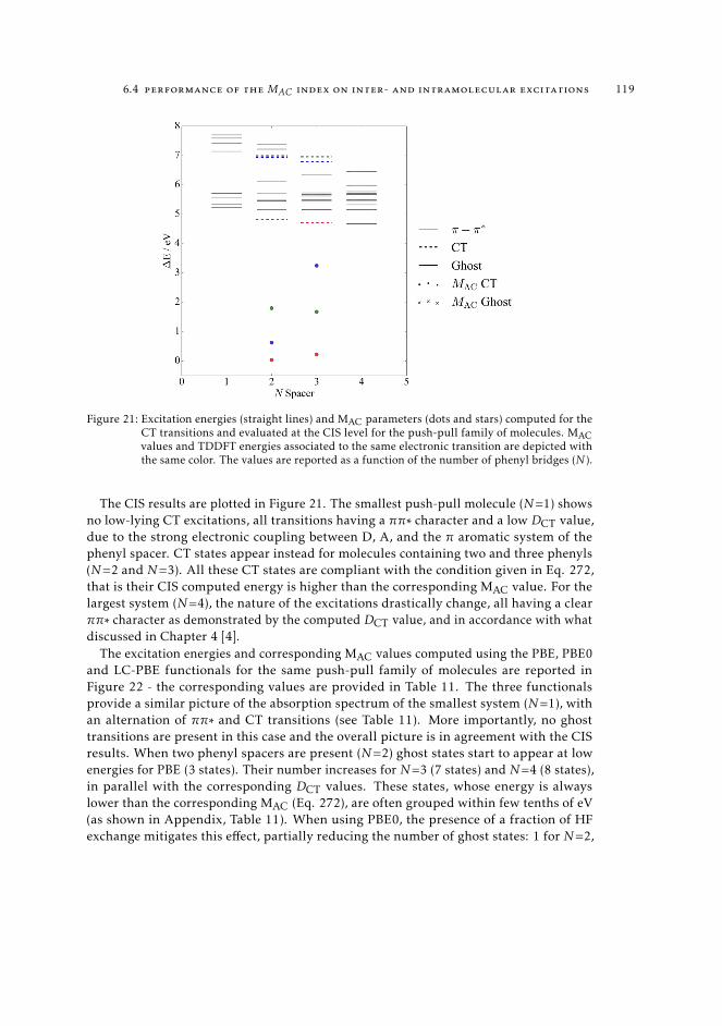
6.4 performance of the MAC index on inter- and intramolecular excitations 119
Figure 21: Excitation energies (straight lines) and MAC parameters (dots and stars) computed for theCT transitions and evaluated at the CIS level for the push-pull family of molecules. MACvalues and TDDFT energies associated to the same electronic transition are depicted withthe same color. The values are reported as a function of the number of phenyl bridges (N ).
The CIS results are plotted in Figure 21. The smallest push-pull molecule (N=1) showsno low-lying CT excitations, all transitions having a ππ∗ character and a low DCT value,due to the strong electronic coupling between D, A, and the π aromatic system of thephenyl spacer. CT states appear instead for molecules containing two and three phenyls(N=2 and N=3). All these CT states are compliant with the condition given in Eq. 272,that is their CIS computed energy is higher than the corresponding MAC value. For thelargest system (N=4), the nature of the excitations drastically change, all having a clearππ∗ character as demonstrated by the computed DCT value, and in accordance with whatdiscussed in Chapter 4 [4].
The excitation energies and corresponding MAC values computed using the PBE, PBE0and LC-PBE functionals for the same push-pull family of molecules are reported inFigure 22 - the corresponding values are provided in Table 11. The three functionalsprovide a similar picture of the absorption spectrum of the smallest system (N=1), withan alternation of ππ∗ and CT transitions (see Table 11). More importantly, no ghosttransitions are present in this case and the overall picture is in agreement with the CISresults. When two phenyl spacers are present (N=2) ghost states start to appear at lowenergies for PBE (3 states). Their number increases for N=3 (7 states) and N=4 (8 states),in parallel with the corresponding DCT values. These states, whose energy is alwayslower than the corresponding MAC (Eq. 272), are often grouped within few tenths of eV(as shown in Appendix, Table 11). When using PBE0, the presence of a fraction of HFexchange mitigates this effect, partially reducing the number of ghost states: 1 for N=2,
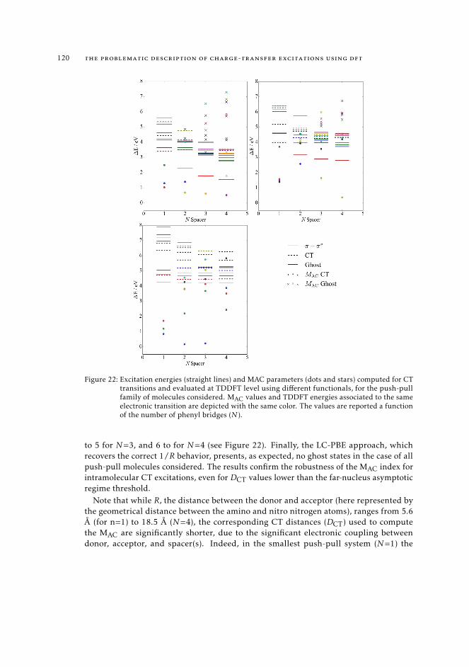
120 the problematic description of charge-transfer excitations using dft
Figure 22: Excitation energies (straight lines) and MAC parameters (dots and stars) computed for CTtransitions and evaluated at TDDFT level using different functionals, for the push-pullfamily of molecules considered. MAC values and TDDFT energies associated to the sameelectronic transition are depicted with the same color. The values are reported a functionof the number of phenyl bridges (N ).
to 5 for N=3, and 6 to for N=4 (see Figure 22). Finally, the LC-PBE approach, whichrecovers the correct 1/R behavior, presents, as expected, no ghost states in the case of allpush-pull molecules considered. The results confirm the robustness of the MAC index forintramolecular CT excitations, even for DCT values lower than the far-nucleus asymptoticregime threshold.
Note that while R, the distance between the donor and acceptor (here represented bythe geometrical distance between the amino and nitro nitrogen atoms), ranges from 5.6Å (for n=1) to 18.5 Å (N=4), the corresponding CT distances (DCT) used to computethe MAC are significantly shorter, due to the significant electronic coupling betweendonor, acceptor, and spacer(s). Indeed, in the smallest push-pull system (N=1) the
6.5 mAC diagnostics in real systems 121
largest computed DCT value is 2.0 Å (for the first CT transition), while the highest valueis computed for the tenth transition in the largest molecules (N=4, DCT 6.6 Å). Thus,both values remain considerably small compared to geometrical distance between thedonor and acceptor fragments. It follows that the correct evaluation of the effectiveCT distance (using the DCT) over the use of a simple geometrical distance is of crucialimportance, especially in the case of systems possessing intramolecular CT excitations,where electron delocalization/conjugation can play a relevant role. Finally, it is worthstressing that especially higher energy excitations can possess a non-negligible multi-determinant character so that the weighted average, performed when computing the MACindex, is relevant for a correct estimation of IP and EA.
In summary, the discussion above substantiates the effectiveness of MAC index in de-tecting ghost CT states, a major problem in TDDFT calculations. The systems investigatedhere are representative of both intermolecular and intramolecular CT excitations. Besides,they comprise both charge-transfer states which fall within and beyond the far-nucleusasymptotic regime defined by Hirao, i.e., where donor and acceptor have a non-negligibleoverlap. Overall, the the MAC index allows detecting the presence of ghost states, alsoin the case where the electronic features of the molecules (i.e., electronic delocalization)do not allow for an a-priori geometrical evaluation of the donor–acceptor distance. Thewidespread use of GGA and GH functionals, many of them providing accurate electronicabsorption energies for valence excitations, can be made “safer” by the use of this de-scriptor. Of note, the evaluation of this index is rather computationally inexpensive.Although the discussion above is based on the results obtained strictly using relaxeddensities [138] - as previously discussed in Chapter 4, we may in principle attempt toperform a similar analysis using unrelaxed densities as well. This last approach can beparticularly convenient, just think of the advantage of computing the MAC diagnostics onall vertical states at once, rather than compute the relaxed density of each. The effect ofusing relaxed/unrelaxed density is discussed more in depth in the following sections.
6.5 mAC diagnostics in real systems
6.5.1 First step to build an effective strategy for the characterization of photochemical processes
In the context of designing density-based strategies to draw a detailed understanding ofexcited state processes, the the MAC index is particularly convenient.
Any method giving access to the energy and the electronic density can be used for theevaluation of density-based descriptors, the only critical point concerning its reliability. Ifthe method used to determine the density is inaccurate, the ensuing observables will beclearly biased. In this respect, the MAC diagnostics can be used to perform a preliminaryanalysis to ensure the correctness of the potential energy curves of the excited states ofinterest. Once this verification is completed, the quest of finding a strategy to describephotochemical processes can be pursued: one can apply other topological descriptorsto characterize the nature of the calculated excited states and, for instance, investigatedifferent regions of the potential energy surfaces of interest.
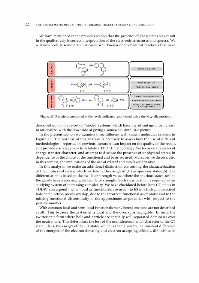
122 the problematic description of charge-transfer excitations using dft
We have mentioned in the previous section that the presence of ghost states may resultin the qualitatively incorrect interpretation of the electronic structures and spectra. Wewill now look at some practical cases, well known photochemical reactions that havebeen previously studied both at the theoretical and experimental level, through which wecan better appreciate the qualities and deficiencies of our index. The diagnostic analysis
N
N
NMe2 N
N
NMe2
τ = 0° τ = 9 0°
hν
N N54
1
6
32
N N 12
354
6
hν
1
2 3
41
2 3
4
τ = 0° τ = 9 0°
N NOH N N
OH
hν
CPD
NO
DM
AB
NPh
en-P
EN
ME
2
PBE0/6-31G(d) - GAS
PBE0/6-31+G(d) - GAS
PBE0/6-311+G(d,p) - CH3CN
CAM-B3LYP /6-31+G(d) - GAS
CAM-B3LYP /6-311+G(d,p) - CH3CN
LC-PBE, CIS, CAM-B3LYP, PBE0 6-31+G(d,p) - CH3CN
Figure 23: Reactions computed at the levels indicated, and tested using the MAC diagnostics.
described up to now resort on "model" systems, which have the advantage of being easyto rationalize, with the downside of giving a somewhat simplistic picture.
In the present section we examine three different well known molecular systems inFigure 23. The purpose of this analysis is precisely to assess how the use of differentmethodologies - reported in previous literature, can impact on the quality of the result,and provide a strategy how to validate a TDDFT methodology. We focus on the states ofcharge-transfer character, and attempt to disclose the presence of unphysical states, independence of the choice of the functional and basis set used. Moreover we discuss, alsoin this context, the implications of the use of relaxed and unrelaxed densities.
In this analysis, we make an additional distinction concerning the characterizationof the unphysical states, which we label either as ghost (G) or spurious states (S). Thedifferentiation is based on the oscillator strength value, where the spurious states, unlikethe ghosts have a non negligible oscillator strength. Such classification is required whenstudying system of increasing complexity. We have elucidated before how CT states inTDDFT correspond - when local xc functionals are used - to ES in which photoexcitedhole and electron poorly overlap, due to the incorrect functional asymptotic and to themissing functional discontinuity of the approximate xc-potential with respect to theparticle number.
With common local and semi-local functionals many bound excitons are not describedat all. This because the xc-kernel is local and the overlap is negligible. In turn, thezwitterionic form where hole and particle are spatially well separated dominates overthe neutral one. This determines the loss of the multideterminantal character of the CTstate. Thus, the energy of the CT states which is then given by the constant differenceof the energies of the electron donating and electron-accepting orbitals, diminishes so
6.5 mAC diagnostics in real systems 123
significantly that these states become the lowest in the calculated electronic spectra. Ifadding exact exchange improves the results, the partial addition of some fraction of exactexchange, may only mitigate these deficiencies, resulting in an only partial correction.As a result, in real systems, the spectrum of unphysical-low-lying states counts of stateswhose degree of error can be of different significance, depending on the particle/holeoverlap [24, 121]. Hence, there might be excited states of CT character which have nonvanishing oscillator strength, but still appear too low in energy. These are the ones werefer to as "spurious". As we discuss in the following, deciding whether a state shall bediscarded or not can be a hard task, as these intermediate cases may be difficult to judge.
There is an additional refinement that we can consider, to recover the correct energyplacement of the vertical states, and precisely to get a better estimate of the virtual orbitalenergy values, εa. As previously mentioned, εa values are fairly wrong when DFAs areused, due to the fact that virtual KS orbitals are one-electron states, which resent the exactsame local potential as the occupied orbitals. In Hartree-Fock instead, the potential forthe virtual orbitals is devoid of the stabilizing hole potential. As a result, the εa orbitals"see" one electron more than the corresponding occupied ones - this is indeed the reasonwhy Hartree-Fock virtual orbitals are more dimly bound, and therefore appear to be morediffuse.
A simple scheme to rectify the underestimation of the eigenvalues of the TDDFT-virtual orbitals is to compute the Hartree-Fock energies, for each given TDDFT densitydistribution. The procedure is easy and fast, as it requires simply to perform a single self-consistent field cycle on top of the converged Kohn-Sham orbitals. The newly obtainedorbital energies are now corrected, and the virtual orbitals are shifted higher in energy,compared to the original KS orbitals. As only one SCF cycle is performed, the overall shapeof the orbitals remains unchanged. Hence, based on these observations we reformulate Eq.271 as,
MAC =∑ia
c2ia(εDFA−HFa − εDFA−HF
i )∑ia c
2ia
− 1DCT
. (274)
As the correction basically affects only the unoccupied orbitals, equations 271 and 274only differ by the amount in which virtual orbitals are lower in DFT than in Hartree-Fock.As a result, Hartree-Fock-corrected MAC values are by definition greater or equal to theoriginal value.
As the subject of our investigations, and particularly of this chapter is rather method-ological than focused on mechanistic details, we will overlook - for now - describing thecharacteristics of the photo-induced processes which occur on the molecules on whichwe apply the MAC diagnostics. We will here limit the discussion to few details necessaryfor our purposes, and refer to the next chapters - and dedicated references - for a morecomprehensive discussion of reactions themselves.
124 the problematic description of charge-transfer excitations using dft
6.5.2 Excited state intramolecular proton transfer in CPDNO
The cyclopropyldiazo-2-naphthol (CPDNO) molecule is a hydrogen-bonded azo-aromaticsystem, which undergoes an intramolecular proton-transfer reaction at the excited state[188]. The reaction connects, at the excited state, the ES-enol∗ to the ketone∗ form (Scheme23). We consider the lowest excited levels and verify the correctness of the energy andnature of the excited states along the reaction coordinate, through the MAC diagnostic.A convenient way to do so is to construct different structures - eight in the present -reasonably close one another, in which the H atom progressively shifts away from theenol-oxygen towards the nitrogen in steps of 0.1 Å.
On these structures we calculate the ten lowest vertical excited states using a globalhybrid coupled with the 6-31G(d) basis-set - corresponding data are available in Appendix,in Table 12. Despite the rather small basis set, and the "standard" choice of functional,such methodology well reproduces the potential-energy curves of the lowest singletstates, in particular, S0, S1, and S2). All values in Appendix, Table 12 are equivalentto those calculated using B3LYP functional coupled with a larger basis-set [163]. Thecomputed surfaces and spectra are also in close agreement with those computed at theCASSCF/CASPT2 [3, 163] level, and are consistent with the experimentally observedphotoproducts. Thus, we expect the computed MAC index to reveal few or no ghost, atleast when relaxed densities are taken into account.
Each panel in Figure 24 represents the computed relaxed and unrelaxed DCT values,for the ten lowest excited states, at different structures (S001 to S008). The vertical statesare labeled according to the computed MAC value and character. Excited states possessingan energy value greater than their associated MAC are classified as charge-transfer orlocally excited states, based on their DCT value. DCT values below 2.0 Å are connotativeof a spatially localized excited state "L", while DCT values greater or equal to 2.0 Å areconsidered as "CT" transitions. Besides, excited states appearing at energy values lowerthan the corresponding MAC are classified either as ghost "G" states if their oscillatorstrength value is below 0.001 or as spurious "S" otherwise.
Figure 24 reveals the presence of few spurious states - light blue scatters, 3rd and 9thvertical excited at reaction steps S001 and S002 and the first and 7th vertical positions atS005 and S006, to name a few. Additionally a number of ghost states (in orange) appear.All these states have large UDCT value, ranging between 2.985 and 3.945 Å (raw data areavailable in Table 12 in Appendix). As such, the charge-transfer character of such states,as calculated with the PBE0/6-31G(d) method is clearly overestimated. The totality ofthese spurious states - only exception the S9/S8 excited state - turn into L states whenthe density relaxation is taken into account. Accordingly, the DCT shrinks by half of thevalue.
The presence of such states, is ascribed to the combination PBE0/6-31G(d) whichcan only describe non-local effects limitedly. As a result, the effect of the relaxationis significant, and one should be careful in judging the G or S nature of the excitedstates using unrelaxed densities. The PBE0/6-31G(d) method remains a valid choice to
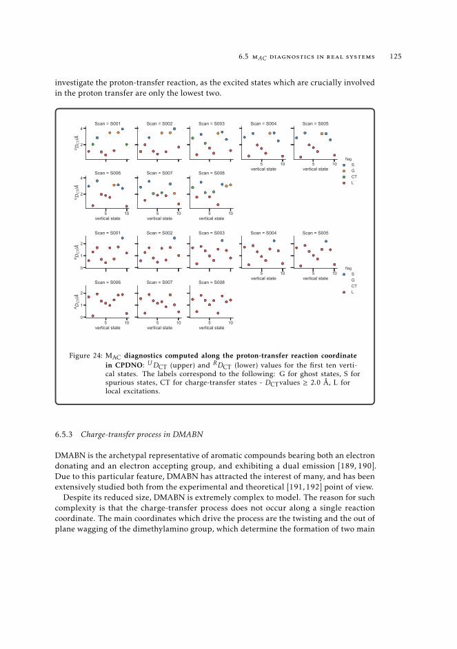
6.5 mAC diagnostics in real systems 125
investigate the proton-transfer reaction, as the excited states which are crucially involvedin the proton transfer are only the lowest two.
2
4
UD
CT/Å
Scan = S001 Scan = S002 Scan = S003
5 10vertical state
Scan = S004
5 10vertical state
Scan = S005
5 10vertical state
2
4
UD
CT/Å
Scan = S006
5 10vertical state
Scan = S007
5 10vertical state
Scan = S008
flagSGCTL
0
1
2
RD
CT/Å
Scan = S001 Scan = S002 Scan = S003
5 10vertical state
Scan = S004
5 10vertical state
Scan = S005
5 10vertical state
0
1
2
RD
CT/Å
Scan = S006
5 10vertical state
Scan = S007
5 10vertical state
Scan = S008
flagSGCTL
Figure 24: MAC diagnostics computed along the proton-transfer reaction coordinatein CPDNO: UDCT (upper) and RDCT (lower) values for the first ten verti-cal states. The labels correspond to the following: G for ghost states, S forspurious states, CT for charge-transfer states - DCTvalues ≥ 2.0 Å, L forlocal excitations.
6.5.3 Charge-transfer process in DMABN
DMABN is the archetypal representative of aromatic compounds bearing both an electrondonating and an electron accepting group, and exhibiting a dual emission [189, 190].Due to this particular feature, DMABN has attracted the interest of many, and has beenextensively studied both from the experimental and theoretical [191, 192] point of view.
Despite its reduced size, DMABN is extremely complex to model. The reason for suchcomplexity is that the charge-transfer process does not occur along a single reactioncoordinate. The main coordinates which drive the process are the twisting and the out ofplane wagging of the dimethylamino group, which determine the formation of two main
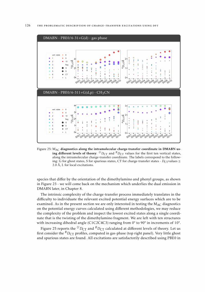
126 the problematic description of charge-transfer excitations using dft
DMABN - PBE0/6-31+G(d) - gas phase
S001S002
S003S004
S005S006
S007S008
S009S010
0
2
4
UD
CT/Å
vert. state
1
2
3
4
5
6
7
8
9
10
flag
G
S
CT
L
S001S002
S003S004
S005S006
S007S008
S009S010
0
1
2
RD
CT/Å
DMABN - PBE0/6-311+G(d,p) - CH3CN
S001S002
S003S004
S005S006
S007S008
S009S010
0
1
2
3
4
UD
CT/Å
vert. state
1
2
3
4
5
6
7
8
9
10
flag
G
S
CT
L
S001S002
S003S004
S005S006
S007S008
S009S010
0
1
2
3
RD
CT/Å
Figure 25: MAC diagnostics along the intramolecular charge-transfer coordinate in DMABN us-ing different levels of theory: UDCT and RDCT values for the first ten vertical states,along the intramolecular charge-transfer coordinate. The labels correspond to the follow-ing: G for ghost states, S for spurious states, CT for charge-transfer states - DCTvalues ≥2.0 Å, L for local excitations.
species that differ by the orientation of the dimethylamino and phenyl groups, as shownin Figure 23 - we will come back on the mechanism which underlies the dual emission inDMABN later, in Chapter 8.
The intrinsic complexity of the charge-transfer process immediately translates in thedifficulty to individuate the relevant excited potential energy surfaces which are to beexamined. As in the present section we are only interested in testing the MAC diagnosticson the potential energy curves calculated using different methodologies, we may reducethe complexity of the problem and inspect the lowest excited states along a single coordi-nate that is the twisting of the dimethylamino fragment. We are left with ten structureswith increasing dihedral angle (C1C2C4C3) ranging from 0° to 90° in increments of 10°.
Figure 25 reports the UDCT and RDCT calculated at different levels of theory. Let usfirst consider the RDCT profiles, computed in gas-phase (top right panel). Very little ghostand spurious states are found. All excitations are satisfactorily described using PBE0 in
6.5 mAC diagnostics in real systems 127
combination with the double-ζ basis set, with the exception of the first vertical state as themolecule approaches the orthogonal conformation. For this last, the vanishing overlap ofthe hole and particle orbitals causes the artificial annihilation of oscillator strength, andsubsequent appearance of a ghost state. As a result, we may conclude that the potentialenergy of the first state - as the torsion exceeds 60° - is severely underestimated in energyand displays the wrong oscillator strength.
It must be noticed though that the first two vertical states are energetically well sepa-rated from the third - which according to the MAC diagnostics is correctly represented.This prevents the mixing of the two lowest excited states with the higher ones - corre-sponding data are collected in Table 13 and 14 in Appendix. Hence, the distribution of thelowest vertical states in PBE0 is likely to be correct, despite the energy underestimation.Based on the profiles calculated we would correctly guess which states are populated andin which order, though with the limit of little agreement between the experimental andthe calculated spectra.
The MAC diagnostics warns us about the limits of the methodology of our choice andwhich are the errors we might incur in. We might still decide to employ a GH-GGAfunctional as PBE0, though due caution is advised. Now let us asses impact of the use ofrelaxed and unrelaxed densities on the MAC diagnostic, by looking at the curves in theupper panel of Figure 25. The RDCT and UDCT profiles point out in the same direction;unrelaxed densities though result in larger DCT values. This in turn can lead to anoverestimation of the presence of ghost states when unrelaxed densities are used. In thisrespect, the use of a large basis-set is convenient - see the RDCT and UDCT profiles inthe bottom panel of Figure 25. These last are calculated using a triple-ζ basis-set andwith added diffuse and polarization functions, and appear to be less subject to variationsas compared with the curves in the upper panel, which are calculated using a double-ζbasis-set (6-31G(d)). Hence, to parity of functional used, larger basis-set render a moreuniform distribution of the DCT curves so that unrelaxed densities can be used instead ofrelaxed ones. Besides, this improved description is also assisted by the addition of solventeffects. The solvent of choice, acetonitrile, is a polar aprotic one, with reduced ability toform hydrogen bonds. Hence, the acetonitrile environment maintains the free torsionaround the triple bond axis and allows the formation of both emissive species.
We conclude that the use of the large base set, together with the solvent effects, isbeneficial, as it allows the use of non-relaxed densities instead of the relaxed ones, withthe advantage that goes with it. The improvement, though is not such to eliminate the CTproblem. As discussed above, the incorrect description of CT states has a well-definedorigin, that is the incorrect shape of the potential energy curve computed using DFT. Theuse of diffuse functions does not compensate the missing overlap of the hole and particleorbitals, not even in a system of such reduced size.
6.5.4 Charge-transfer process in Phen-PENMe2
Finally we examine the charge-transfer process in 5-(4-dimethylaminophenylenylethylyn)-1,10-phenanthroline, Phen-PENMe2 in abbreviated form. We discuss in detail the photo-
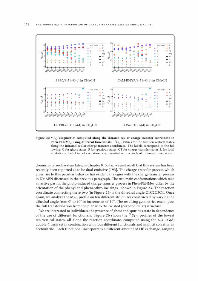
128 the problematic description of charge-transfer excitations using dft
S001S002
S003S004
S005S006
S007S008
S009S010
0
2
4
6
8
UD
CT/Å
vert. state1234567
8910flagGSCTL
PBE0/6-31+G(d) in CH3CN
S001S002
S003S004
S005S006
S007S008
S009S010
2
4
6
UD
CT/Å
vert. state1234567
8910flagGSCTL
CAM-B3LYP/6-31+G(d) in CH3CN
S001S002
S003S004
S005S006
S007S008
S009S010
0
1
2
3
4
UD
CT/Å
vert. state1234567
8910flagGCTL
LC-PBE/6-31+G(d) in CH3CN
S001S002
S003S004
S005S006
S007S008
S009S010
0
1
2
3
UD
CT/Å
vert. state1234567
8910flagSCTL
CIS/6-31+G(d) in CH3CN
Figure 26: MAC diagnostics computed along the intramolecular charge-transfer coordinate inPhen-PENMe2 using different functionals: UDCT values for the first ten vertical states,along the intramolecular charge-transfer coordinate. The labels correspond to the fol-lowing: G for ghost states, S for spurious states, CT for charge-transfer states, L for localexcitations. Each kind of excitation is represented with a circle of different dimensions.
chemistry of such system later, in Chapter 8. So far, we just recall that this system has beenrecently been reported as to be dual emissive [193]. The charge-transfer process whichgives rise to this peculiar behavior has evident analogies with the charge-transfer processin DMABN discussed in the previous paragraph. The two main conformations which takean active part in the photo-induced charge-transfer process in Phen-PENMe2 differ by theorientation of the phenyl and phenanthroline rings - shown in Figure 23. The reactioncoordinate connecting these two (in Figure 23) is the dihedral angle C1C2C3C4. Onceagain, we analyze the MAC profile on ten different structures constructed by varying thedihedral angle from 0° to 90° in increments of 10°. The resulting geometries encompassthe full transformation from the planar to the twisted (perpendicular) structure.
We are interested to individuate the presence of ghost and spurious state in dependenceof the use of different functionals. Figure 26 shows the UDCT profiles of the lowestten vertical states, all along the reaction coordinate, computed using the 6-31+G(d)double-ζ basis set in combination with four different functionals and implicit solvation inacetonitrile. Each functional incorporates a different amount of HF exchange, ranging
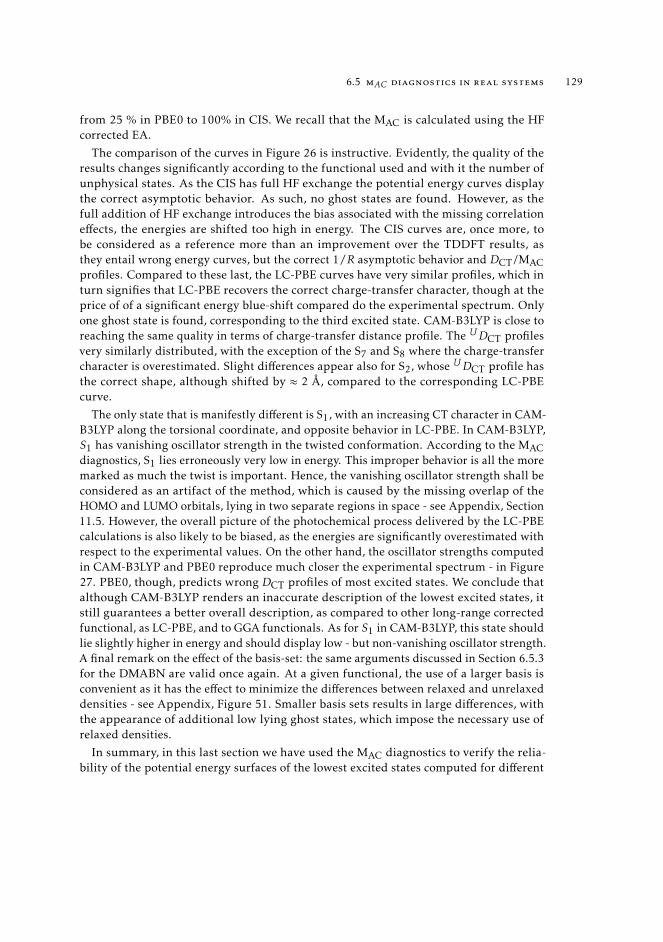
6.5 mAC diagnostics in real systems 129
from 25 % in PBE0 to 100% in CIS. We recall that the MAC is calculated using the HFcorrected EA.
The comparison of the curves in Figure 26 is instructive. Evidently, the quality of theresults changes significantly according to the functional used and with it the number ofunphysical states. As the CIS has full HF exchange the potential energy curves displaythe correct asymptotic behavior. As such, no ghost states are found. However, as thefull addition of HF exchange introduces the bias associated with the missing correlationeffects, the energies are shifted too high in energy. The CIS curves are, once more, tobe considered as a reference more than an improvement over the TDDFT results, asthey entail wrong energy curves, but the correct 1/R asymptotic behavior and DCT/MACprofiles. Compared to these last, the LC-PBE curves have very similar profiles, which inturn signifies that LC-PBE recovers the correct charge-transfer character, though at theprice of of a significant energy blue-shift compared do the experimental spectrum. Onlyone ghost state is found, corresponding to the third excited state. CAM-B3LYP is close toreaching the same quality in terms of charge-transfer distance profile. The UDCT profilesvery similarly distributed, with the exception of the S7 and S8 where the charge-transfercharacter is overestimated. Slight differences appear also for S2, whose UDCT profile hasthe correct shape, although shifted by ≈ 2 Å, compared to the corresponding LC-PBEcurve.
The only state that is manifestly different is S1, with an increasing CT character in CAM-B3LYP along the torsional coordinate, and opposite behavior in LC-PBE. In CAM-B3LYP,S1 has vanishing oscillator strength in the twisted conformation. According to the MACdiagnostics, S1 lies erroneously very low in energy. This improper behavior is all the moremarked as much the twist is important. Hence, the vanishing oscillator strength shall beconsidered as an artifact of the method, which is caused by the missing overlap of theHOMO and LUMO orbitals, lying in two separate regions in space - see Appendix, Section11.5. However, the overall picture of the photochemical process delivered by the LC-PBEcalculations is also likely to be biased, as the energies are significantly overestimated withrespect to the experimental values. On the other hand, the oscillator strengths computedin CAM-B3LYP and PBE0 reproduce much closer the experimental spectrum - in Figure27. PBE0, though, predicts wrong DCT profiles of most excited states. We conclude thatalthough CAM-B3LYP renders an inaccurate description of the lowest excited states, itstill guarantees a better overall description, as compared to other long-range correctedfunctional, as LC-PBE, and to GGA functionals. As for S1 in CAM-B3LYP, this state shouldlie slightly higher in energy and should display low - but non-vanishing oscillator strength.A final remark on the effect of the basis-set: the same arguments discussed in Section 6.5.3for the DMABN are valid once again. At a given functional, the use of a larger basis isconvenient as it has the effect to minimize the differences between relaxed and unrelaxeddensities - see Appendix, Figure 51. Smaller basis sets results in large differences, withthe appearance of additional low lying ghost states, which impose the necessary use ofrelaxed densities.
In summary, in this last section we have used the MAC diagnostics to verify the relia-bility of the potential energy surfaces of the lowest excited states computed for different
130 the problematic description of charge-transfer excitations using dft
250 300 350 400 450 500 / nm
0.0
0.2
0.4
0.6
0.8
/ L
mol
1 cm
1
1e5= 0° CAM-B3LYP= 90° CAM-B3LYP= 0 90° CAM-B3LYP= 0° LC-PBE= 90° LC-PBE= 0 90° LC-PBE
experimental EtOH
Figure 27: Comparison of the calculated absorption spectra of Phen-PENMe2 - both in CAM-B3LYPand LC-PBE in CH3CN and experimentally.
molecular systems, such as CPDNO, DMABN and Phen-PENMe2. Here, we have ulteriorlyrefined the formulation of our index by introducing a mixed DFT-HF correction, yielding abetter estimate for the energies of the virtual orbitals, which are typically underestimatedusing density functional approximations. Using our index we were able to identify thepresence of ghost and spurious states, and to characterize all other excitations as havinglocal or charge-transfer character. We have shown how the presence of ghost states canaffect the interpretation of the excited state process and how our diagnostic analysis canbe used for this purpose. Spurious states are not as critical as ghost states as they corre-spond to excited levels that are only partially mistaken by the method of choice. Relaxeddensities in general provide better description of excited states possessing CT character.However, for the same density functional approximation the use of a larger basis set canbe beneficial as it has the effect to mitigate the differences between the pictures obtainedby using relaxed or unrelaxed densities. This observation supports the use of unrelaxeddensities, instead of the more onerous relaxed ones.
7MAC DIAGNOST ICS IN METAL COMPLEXES
7.1 context
The many controversies regarding the use of TDDFT for long-range charge-transfer ex-cited states extend to metal-complexes as well. The prediction of the nature and propertiesof excited states of transition metal complexes is a fertile research area [194–196]. Due totheir rather peculiar photochemical and photophysical properties, organometallic com-plexes of several metals are nowadays exploited in different fields and applications [197].In particular, ruthenium complexes have been the basic components of dye-sensitized-solar cells from the very beginning of such technology and are still today among the mostefficient dyes [23].
In a totally different field, ruthenium complexes have been largely applied as DNAprobes, since they have a demonstrated ability to establish strong interaction with suchmacromolecule [198]. In fact, it has been shown that the photophysical properties of thecomplexes change radically upon interaction with DNA and the fluorescence can be tunedby the environment in which the complexes are immersed [199, 200]. In some cases, thefluorescence present in aqueous media, is quenched by DNA interaction [201], while inother cases dark solvated compounds show an intense fluorescence upon the addition ofDNA. The high DNA binding affinity and unique light-switch effect of Ru complexes makethem attractive compounds not only to investigate metal-to-biomolecules interactions, butalso for related research areas such as sensitive diagnostics, chemotherapeutics, and photo-therapy [195]. Indeed, ruthenium complexes have known potential as antitumoral drugs,as they cause irreversible DNA damage through intercalation and subsequent excitedstate mediated charge-transfer process. In the field of biochemistry, the luminescence ofRu(II) complexes has also been observed in non-polar environment, such as hydrophobiccavities in proteins. These are only few of the many existing applications [202].
Processes of such intrinsically complex nature, are extremely interesting to study, yetdifficult to understand based on sole experimental investigations. Indeed a good un-derstanding of the photophysical processes involved in such phenomena is critical torecognize and improve the therapeutic properties of such systems. This is also the reasonwhy such compounds, and especially Ru complexes, are the object of numerous of studiesbased on theoretical computations and spectroscopic techniques. Actually, the use oftheoretical methods is crucial to correctly model the behavior of such complexes uponirradiation, and to acquire a realistic description of their excited state manifold [24].Transition metal complexes cumulate most of the complexities inherent to theoreticalstudies: size, electronic delocalization, high density of electronic states of various char-acters, multi-reference nearly degenerate states, long-range charge-transfer states and
131
132 mAC diagnostics in metal complexes
vibronic couplings. Moreover as the d and f shells become populated, relativistic effects,spin–orbit coupling, dissociative states, and states mixing become important.
With the aim of setting up computational protocols enabling to accurately predict anddescribe the nature and energetics of the excited states, specific quantum methods havebeen explicitly devised and benchmarked on metal containing complexes. Among these,the most popular methodologies used to treat these systems are density based methods butalso the variational approaches based on the self-consistent- field (SCF) formalism and itsmulti-configuration extension complete-active-space SCF (CASSCF) [168] or the variantsrestricted- active-space SCF (RASSCF) [203]. These last have be ulteriorly improved byadding perturbative correction (CASPT2) [169], which allow including of non-dynamicalelectronic correlation effects. If the latter approaches have been proved to yield a highaccuracy in describing both vertical absorption and photochemical behavior of metalcomplexes, these however impose a heavy computational burden which limits theirdomain of applicability to rather small compounds. Moreover, they require the selectionof a relevant system-specific active space, which makes them unpractical and of difficultusage for routine applications.
Hybrid methods have also emerged [204], which combine DFT at short-range, and wavefunction or perturbative approaches at long-range. These last, however also suffer fromthe same drawbacks.
TDDFT approaches, on the contrary have the advantage of a favorable scaling, whichhas determined their widespread diffusion in the treatment of metal based complexes.In addition, density rooted approaches limit the user dependency to the choice of theexchange correlation functional to be used, which in practice renders these methodsuncomplicated, though impressively accurate in the description of structural and spectro-scopic properties of transition metal complexes, at least for what concerns the electronicground state and the lowest excited states. Not surprisingly, TDDFT calculations and sim-ulated spectra obtained from them are increasingly used to support experimental findings,where the actual characterization of the nature of the observed transition by electronicstructure calculations can provide an extremely valuable addition and reinforcement tothe experimental studies [24, 205, 206].
For these comparative studies, usually the choice of the exchange correlation functionalis based on previous works dealing with similar compounds, showing a good agreementwith the experimental results. However, matching experimental/theoretical spectra mayjust arise because of a lucky compensation of errors. Indeed, the limitation of DFT andTDDFT, apply to metal containing complexes too. The wrong asymptotics typical of localexchange functionals has severe consequence on the computed excitation energies of suchclass of compounds, which in turn, may strongly affect the predicted photophysical andphotochemical properties, and with it the interpretation of the mechanism of the relatedexcited state processes. Therefore, a note of caution is needed. In particular, transitionmetal complexes are often designed with the precise purpose of enhancing the CT char-acter in the electronic ground stater, or in the lowest excited state, to obtain compoundspossessing a low absorption wavelength and a high molar extinction coefficient simultane-ously. For instance, compounds with such properties are extensively researched in the
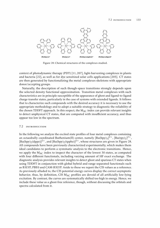
7.2 introduction 133
N
N
N
NRu2+
N
NN
N
N
N
N
NRu2+
N
NN
N
NN
N
N
N
NRu2+
N N
N
N
N
NRu2+
N N
[Ru(bpy)3]2+ [Ru(tpy)2]2+ [Ru(bpy)2(tpphz)]2+ [Ru(bpy)2(dppz)]2+
Figure 28: Chemical structures of the complexes studied.
context of photodynamic therapy (PDT) [11, 207], light-harvesting complexes in plantsand bacteria [22], as well as for dye sensitized solar cells applications [205]. CT statesare then generated by functionalizing the metal complexes skeletons with appropriatedonor/accepting groups.
Naturally, the description of such though-space transitions strongly depends uponthe selected density functional approximation. Transition metal complexes with suchcharacteristics are in principle susceptible of the appearance of ghost and ligand-to-ligandcharge-transfer states, particularly in the case of systems with extended ligands. It followsthat to characterize such compounds with the desired accuracy it is necessary to use theappropriate methodology and to adopt a suitable strategy to diagnostic the reliability ofthe chosen TDDFT approach. In this respect, the MAC index can provide relevant insightsto detect unphysical CT states, that are computed with insufficient accuracy, and thusappear too low in the spectrum.
7.2 introduction
In the following we analyze the excited state profiles of four metal complexes containingan octaedrally coordinated Ruthenium(II) center, namely [Ru(bpy)3]2+, [Ru(tpy)2]2+,[Ru(bpy)2(dppz)]2+, and [Ru(bpy)2(tpphz)]2+, whose structures are given in Figure 28.All compounds have been previously characterized experimentally, which makes themideal candidates to perform a systematic analysis to the electronic transitions. Hence,we apply the MAC index to inspect the character of the lowest 30 states, as computedwith four different functionals, including varying amount of HF exact exchange. Thediagnostic analysis provides relevant insights to detect ghost and spurious CT states whenusing TDDFT in conjunction with global hybrid and range separated functionals suchas B3LYP, PBE0 and CAM-B3LYP. Aside to these we report the CIS values as a reference.As previously alluded to, the CIS potential energy curves display the correct asymptoticbehavior, thus, by definition, CIS MAC profiles are devoid of all artificially low-lyingexcitation. By contrast, the curves are systematically shifted too high in energy. Hence, weinclude these value as a ghost-free reference, though, without discussing the orbitals andspectra calculated from it.
134 mAC diagnostics in metal complexes
The character of an electronically excited state is one of the most important descriptorsemployed to discuss the photophysics and photochemistry of all kinds of molecules,included transition metal complexes. In transition metal complexes, the interactionbetween the metal and the different ligands gives rise to a rich variety of excited states,including metal-centered (MC), ligand-centered (LC), metal-to-ligand-charge transfer(MLCT), ligand-to-metal-charge-transfer (LMCT), intra-ligand-charge-transfer (ILCT),and ligand-to-ligand-charge-transfer (LLCT) states. Most often, these excited statesare identified by considering the most important wave function excitation coefficientsand inspecting visually the involved orbitals. It is therefore clear that, discerning theunphysical spurious transition is of primary importance.
When π-accepting ligands, such as polypyridyl ligands, are coordinated to Ru(II), thecomplex, already in its ground state may exhibit intense singlet-singlet MLCT transitionsin the visible region [208]. This behavior is common for both tris-bidentate and bis-tridentate complexes, although a red-shift of the absorption maximum wavelength isoften observed for the bis-tridentate ones. The molar absorption coefficients for the1MLCT transitions depend on the ability of the ligand to delocalize the excited electronfar from the metal center. Thus, complexes with higher electron accepting capabilitieshave higher molar absorption coefficients. Metal-centered and ligand-centered transitionscan also be identified, in the electronic spectrum.
7.3 analysis of the absorption spectra of ru(ii) polypyridyl complexes
Let as first comment on the absorption profiles of the four selected Ru(II) compounds,in acetonitrile. The normalized experimental absorption spectra - black dotted curve -as well as the simulated spectra, computed using four different functionals are shown inFigure 29. The measured and calculated absorption spectra of [Ru(bpy)3]2+- tB in thefollowing - are qualitatively similar. The broad band around 400-500 nm correspondsto multiple MLCT transitions from the Boltzmann-populated lowest-lying dπ6(Ru) toπ∗(tpy) [209]. The inspection of the NTOs - reported in Appendix, Figure 57 - and thecomputed energy values and oscillator strength - in Appendix, Table 11.7 - allows usto perform a similar assignment of the calculated bands. The most intense peaks in thevisible region correspond to MLCT dπ∗ transitions around 430 nm - excited states 7, 8in B3LYP and PBE0 and slightly higher in energy at ≈ 360 nm - excited states 5,6 - inCAM-B3LYP. As expected, the electronic transitions calculated using GH functionals -PBE0 and B3LYP - better reproduce the measured ones, while range separated functionalsuch as CAM-B3LYP result in a significant blue shift. The CIS spectrum is not even closeto reproducing any of the features of the experimental spectrum and is irrecoverablyblue-shifted. These general trends apply analogously to [Ru(tpy)2]2+- referred to as bTlater on. Analogously, the lowest bright transitions correspond to MLCT dπ∗ transitions,which appear at around 450 nm in PBE0 and B3LYP and slightly higher in energy, at ≈390 nm in CAM-B3LYP.
The experimental absorption spectra of the substituted cyclometalated complexesRu[(bpy)2(dppz))]2+ and Ru[(bpy)2(tpphz))]2 - D and T in the following - are character-
7.4 mAC diagnostics in metal complexes 135
ized by an intense band centered at 290 nm corresponding to a strong absorption of theligand-centered (LC) excited states and a weak absorption around 370 nm, which canbe assigned to the metal centered (MC) transitions [210]. This shoulder is more intensein the dppz-substituted complex than in the [Ru(bpy)2(tpphz)]2+substituted one, as inthis last the LC transitions propagate at lower energy and rise above the week metalcentered bands. In contrast with the homoleptic complexes discussed above, D and Tdo not exhibit the tail of the visible band - extending towards 600 nm in tB and bT , andtypical of the cyclometalated complexes that absorb between 400 nm and 550 nm in thelow-lying metal-to-ligand-charge-transfer (MLCT) excited states.
In the B3LYP and PBE0 computed absorption profiles of D and T the LC band isslightly red-shifted compared to the measured spectra and broader as it incorporates alsothe higher energy intense LC(dppz) and ILCT(dppz) (and LC(tpphz) and ILCT(tpphz)transitions - visible as a shoulder at 260 nm in the experimental spectra.
The spectra of complexes D and T show a large blending of MLCT(dppz -tpphz) /MLCT(bpy) transitions in the visible energy domain with three intense absorptions at 456nm, 423 nm and 415 nm - in the B3LYP spectrum of D - contributing to the large bandbetween 500 nm and 400 nm. The same bands appear in the spectrum of T at 450 nm423 nm and 414 nm, respectively. The comparison between experimental and computedspectra allows us to characterize the different spectral regions, and to assign the mainbands to different kind of excitations, in agreement with previous literature [208,211–213].We can summarize such analysis as follows: as all compounds contain an octaedrallycoordinated Ru center, the absorption spectra display more or less the same features.The lowest energy region is dominated by the MLCT transitions. At higher energy onefinds the LC transitions, i.e. transitions in which an electron is excited in on a ligand andtransferred to a different one. The less intense MC bands lie in between.
7.4 mAC diagnostics in metal complexes
A crucial aspect of the excited states ofD and T complexes is their localization on the dppzand tpphz ligands. In particular, it has been shown that their photochemical properties aretightly bound to the presence of different type of states which localize on distinct regionsof the substituents: some states involve the part of dppz close to the metal atom (normallyreferred to as "proximal" subunit [215]), other involve the other part ("distal" [215]). Theanalysis of absorption profiles is somewhat the standard approach and first step in theinvestigation of the photochemical properties of metal complexes, as it tells which are thelowest dipole allowed transitions. Then, one can perform a full optimization of the lowestabsorbing excited states to determine which excited state contribute to establish the chargedelocalization pathway eventually leading to the emission. This is the main reason whyit is important as a first step to determine which electronic excitations are well modeledby a given method, especially those that are significantly delocalized on the substituents.For instance, MLCT transitions are generally said to be well described by most of thecommonly used DFAs, because of the large degree of overlap between the metal d orbitalsand the accepting orbital on the ligand [24]. By contrast, through-space transitions are
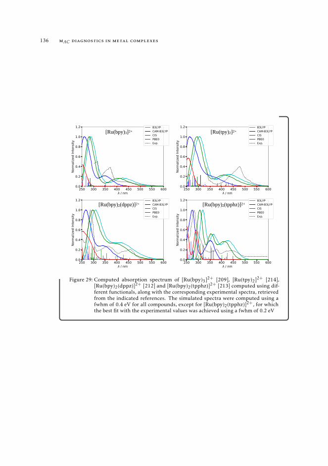
136 mAC diagnostics in metal complexes
[Ru(bpy)3]2+
[Ru(bpy)2(dppz)]2+ [Ru(bpy)2(tpphz)]2+
[Ru(tpy)2]2+
Figure 29: Computed absorption spectrum of [Ru(bpy)3]2+ [209], [Ru(tpy)2]2+ [214],[Ru(bpy)2(dppz)]2+ [212] and [Ru(bpy)2(tpphz)]2+ [213] computed using dif-ferent functionals, along with the corresponding experimental spectra, retrievedfrom the indicated references. The simulated spectra were computed using afwhm of 0.4 eV for all compounds, except for [Ru(bpy)2(tpphz)]2+, for whichthe best fit with the experimental values was achieved using a fwhm of 0.2 eV
7.4 mAC diagnostics in metal complexes 137
susceptible to be wrongly characterized when using standard GH functionals, due to themissing hole-particle overlap. It is therefore important to assess if and which excited statelevels are wrongly described and why. In this respect the MAC diagnostics can be usefulto determine the reliability of a given methodology. The analysis of the lowest 30 states ofthe four metal complexes is reported in Figures 30 and 31, where we report the energylevels and DCT values calculated at four different level of theory. It is important specifythat the DCT values relative to the charge-transfer transition of homoleptic complexesare not null. This observation, in apparent contradiction with the definition of the DCTintroduced in Chapter 3, is however easy to explain. In fact, the CT transitions in tB andbT typically involve the displacement of an electron from the metal center to one of thebipyridine/terpyridine ligands. The charge distributions of these kind of transitions arenot centrosymmetric, therefore yielding non-zero DCT values. Since all ligands in thecoordination sphere are identical any CT occurring on one ligand has the same probabilityto appear on the other ligands. Therefore each CT state is expected to be degenerate atleast as many times as the number of identical subunits in the complex.
Let us start by commenting the results relative to the tB and bT complexes. Theseare homoleptic structures, where the Ru is either coordinated with two tridentate ligand(terpyridine) or with three bidentate ligands (bipyridine). The absence of an asymmetriccharge withdrawing group, results in a reduced variability in the character of the excitedstates, at least for what concerns the lowest 30 singlet excited states. Accordingly, theNTOs - given in Appendix in Figure 56 to 56 - and 57 to 57 are largely dominated by MLCTstates, intercalated by a reduced number of LC states. At higher energy an increasingnumber of MLCT states has mixed MLCT/LLCT character. The apparent absence of MCstates can be traced back to the artificial delocalization of the virtual orbital in DFT, whichin turn makes it difficult to distinguish the MC states from MLCT ones. There is no majordifference given by the use of B3LYP, PBE0 or CAM-B3LYP, hence the excited state profilesof all three functionals are rather close, in both complexes.
As previously alluded to, the MLCT state are usually well described because the degreeof overlap between the metal d orbitals and the π accepting orbitals of the ligand islarge enough. As the excited state manifold of tB and bT is mostly composed by MLCTtransitions - at least up to the 30th transition, we expect the MAC profile to display nospurious and ghost states. The MAC profiles in Figure behave as foreseen, as indeed,no artificially low-lying states are found - at least when relaxed densities are used -independent of the functional chosen. Figure 30 shows the energy levels, UDCT and RDCTvalues of the lowest 30 singlet states of tB and bT , calculated using the four differentfunctionals.
Each state in Figure 30 is assigned a label according to its MAC value, and representedusing markers of different size (or length). As previously discussed in Section 6.5, tran-sitions possessing DCT values below 2.0 Å are denoted as local (L), while those havingDCT values CT greater or equal to to 2.0 Å are supposed to have a charge-transfer (CT)character. Besides, transitions with excitation energy values lower than the correspondingMAC are classified either as ghost (G) states if their oscillator strength value is below 0.001
138 mAC diagnostics in metal complexes
or as spurious (S) otherwise. The size of the corresponding marker in the plot increasesaccording to the following ordering: L, CT, S, G.
As the bpy and tpy ligands are symmetrically distributed in the coordination sphere,they do not immediately cause the appearance of through space charger-transfer states.Therefore, the excited states of tB and bT shall not be concerned by the problems relatedto the description of charge-transfer states. Spurious and ghost states in the UDCT profilesof both tB and bT can be considered as artifacts related to the use of unrelaxed densities.Accordingly, the correct DCT values are restored as soon as relaxed densities are used.Besides, the overestimation of the charge-transfer distance only affects higher excitedstates - S10 or greater, with the only exception of the third excited state of tB. It isimportant to notice that unrelaxed densities deliver almost the same overall pictureas relaxed densities, which in the context of transition metal complexes translates insignificant savings in time and resources.
To fully appreciate the benefits of the diagnostic analysis it is appropriate to apply theMAC index to investigate the electronic transitions of heteroleptic complexes, in whicha ligand is responsible for the delocalization and stabilization of the perturbed chargedistribution that is established upon excitation. D and T complexes are exemplary inthis regard. The Ruthenium atom remains coordinated with three ligands, among which,the primary ligand, here dppz or tpphz, is responsible for the formation of numerouscharge-transfer states. The variety of the transitions increases considerably. Among theMLCTs, some involve the transfer of an electron from the metal center to the ancillaryligands, in the present case the bipyridines. Other MLCT transitions, the more represented,occur between the Ru atom and the main ligand (dppz or tpphz). Among these, furtherdiversification can be made as the transferred charge can be accumulated in differentspecific regions of the ligand - a list of structure and abbreviations is provided in Appendix,Figure 55. Of course, the transition landscape is not limited to MLCTs. The same varietyextends to localized transitions too. MC transitions appear as well. The MAC allows thesystematic cataloging of transitions and identifying of the anomalies related to the use ofan inappropriate functional.
Unlike what occurred for bT and tB, the number of spurious or ghost states - in Figure31 - is consistent. In the following, we try to rationalize the different types of "spurious"states and identify the most problematic ones.
Let us focus on the ghost and spurious states of the D complex. The full list of thecalculated states with excitation energies, oscillator strength and computed MAC values isreported in Appendix, Table 21.
Spurious and ghost states fall into a very specific range of DCT values. This is notsurprising given that these states are associated with an incorrect estimate of the spatialextent of the transition. The DCT values of such states range from 2.2 and 4.2 Å, withthe sole exception of S28 with a DCT value exceeding 5.5 Å. This last, though is not verysignificant, as it lies very high in energy.
The difference between the two panels in Figure 31 is very little, regardless of thefunctional used. Therefore the gain in using relaxed densities is negligible, and an unre-laxed density calculation is fully admitted to discern the presence of any spurious/ghost
7.4 mAC diagnostics in metal complexes 139
state. This observation is in line with what discussed previously in Chapter 6 for smallorganic systems, where we have observed that the oscillation between the values of UDCTand RDCT is only significant when the basis set used is very small, independently of thefunctional.
Most of the states labeled with S or G appear exclusively when functionals containinga low percentage of HF exchange, such as B3LYP and PBE0, are used. The use of CAM-B3LYP drastically reduces their presence. In particular, the analysis reveals a single ghoststate - corresponding to the first excited state, calculated in PBE0 or B3LYP. The densitydifference of this last - in Figure 32 - shows that this state is an MLCT in which the orbitalacceptor is highly delocalized over the entire ligand. Thus, based on the MAC analysis,we deduce that the delocalization is an artifact of the method and this state erroneouslyappears too low in energy.
The same state calculated in CAM-B3LYP is in fact resized and localized on the phenan-throline near the metal center alone - as shown in the NTO analysis in Appendix, inFigure 58. Besides, for the same state, the oscillator strength increases from 0.0001 inPBE0 to 0.002 in CAM-B3LYP. This small value, though, suggests that S1 remains of littlerelevance in absorption, and therefore, does not contribute significantly to the formationof the CT states that populate the emissive state.
The first state that is optically active is the fourth - regardless of the functional used.The diagnostic analysis classifies this state as spurious - when PBE0 or B3LYP are used -as it appears below the limit defined by equation 274. Once again, the difference densityplots reveal that such state is mistakenly delocalized over the whole dppz ligand. Thesame state, calculated in CAM-B3LYP, is again less widespread, although to a lesser extentthan in S1. By contrast, the absorption spectrum calculated in CAM-B3LYP is significantlyblue-shifted compared the calculated spectrum in B3LYP, and differs significantly fromthe experimental one. S4 is responsible for the lowest energy band in the absorptionspectrum. The label S, assigned according to the MAC value suggest that S4 is slightlyoverestimated, and should be therefore treated with caution. The orbital shapes calculatedwith CAM-B3LYP give an idea what the distribution of S4 should resemble to, though thecorrection provided by the range-separated hybrid is too drastic.
In the same vein of the discussion above, one can analyze the spurious excited statesat higher energy. The difference density representation of a selection of states markedas spurious after applying the MAC diagnostic analysis are shown in Figure 32. Thedensity distributions of such states changes as one moves to higher energy. At lowerenergy the spurious states have MLCT character. Gradually the character changes, andthe contributions of the ancillary ligands become more pronounced. Finally the higherspurious states have ILCT character.
We conclude that the electronic transitions calculated using B3LYP and PBE0 are cor-rectly distributed, but slightly underestimated in energy as compared to the experimentaldata. It is evident that the classification of a state as spurious is not as problematic as thatof ghost states. The general image that we derive is that the states classified as spuriousare only partially affected by error and the resulting interpretation is not compromised.

140 mAC diagnostics in metal complexes
These observations hold with no exception for complex T . The extended tpphz liganddetermines an increase in the observed number of ghost/spurious states, independentlyof the functional. The patterns observed for dppz, though, remain unvaried. The lowestexcited state is classified as a ghost. As in complex D this state has MLCT character,with very little overlap between hole and particle orbitals. The inaccuracy of the methodin describing this state has no impact on the study of the photochemical pathway ofthis complex, as this state does not contribute to the absorption and the luminescence isattributed to a state of triplet multiplicity which is accessed upon ISC from the initiallyabsorbing singlet state [194, 208]. Once again the equivalence in the use of U and Rdensities is verified, as the computed UDCT values are only limitedly higher compared tothe relaxed counterparts.
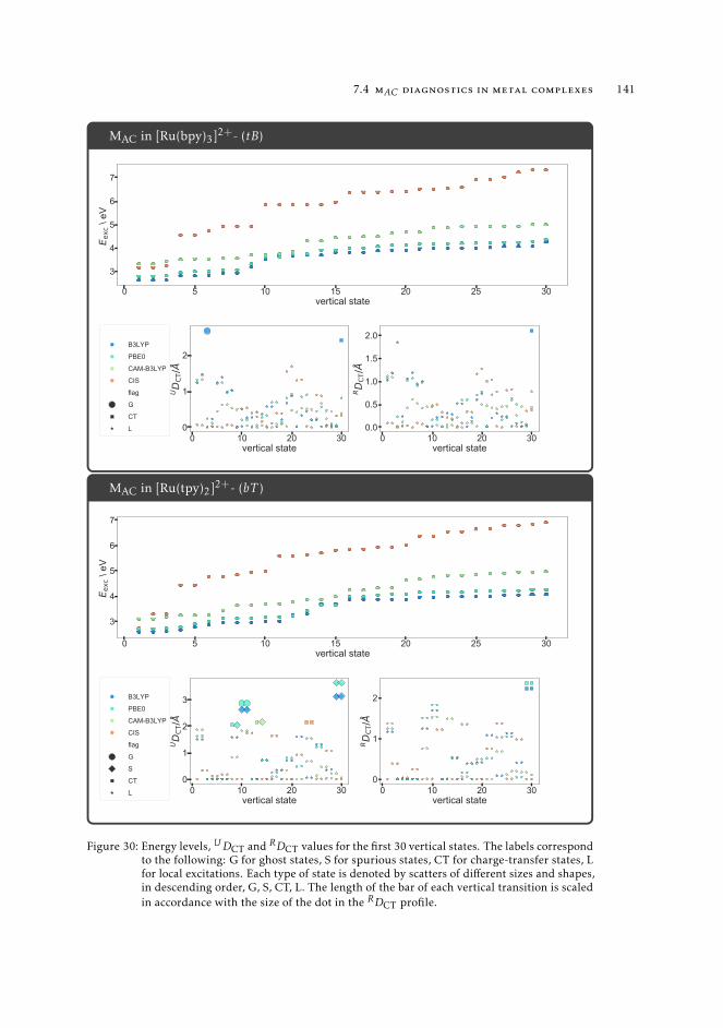
7.4 mAC diagnostics in metal complexes 141
MAC in [Ru(bpy)3]2+- (tB)
0 5 10 15 20 25 30vertical state
3
4
5
6
7
E exc
\ eV
0 10 20 30vertical state
0
1
2
UD
CT/Å
B3LYP
PBE0
CAM-B3LYP
CIS
flag
G
CT
L0 10 20 30
vertical state
0.0
0.5
1.0
1.5
2.0
RD
CT/Å
MAC in [Ru(tpy)2]2+- (bT )
0 5 10 15 20 25 30vertical state
3
4
5
6
7
E exc
\ eV
0 10 20 30vertical state
0
1
2
3
UD
CT/Å
B3LYP
PBE0
CAM-B3LYP
CIS
flag
G
S
CT
L 0 10 20 30vertical state
0
1
2
RD
CT/Å
Figure 30: Energy levels, UDCT and RDCT values for the first 30 vertical states. The labels correspondto the following: G for ghost states, S for spurious states, CT for charge-transfer states, Lfor local excitations. Each type of state is denoted by scatters of different sizes and shapes,in descending order, G, S, CT, L. The length of the bar of each vertical transition is scaledin accordance with the size of the dot in the RDCT profile.
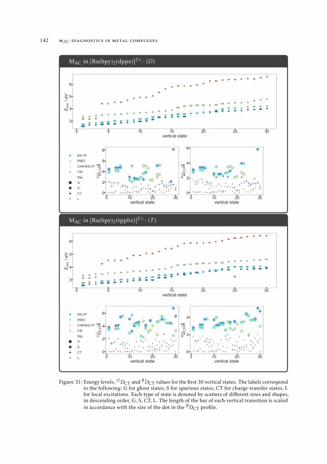
142 mAC diagnostics in metal complexes
MAC in [Ru(bpy)2(dppz)]2+- (D)
0 5 10 15 20 25 30vertical state
3
4
5
6
E exc
\ eV
0 10 20 30vertical state
0
2
4
6
8
UD
CT/Å
B3LYP
PBE0
CAM-B3LYP
CIS
flag
G
S
CT
L 0 10 20 30vertical state
0
2
4
6
RD
CT/Å
MAC in [Ru(bpy)2(tpphz)]2+- (T )
0 5 10 15 20 25 30vertical state
3
4
5
6
E exc
\ eV
0 10 20 30vertical state
0
2
4
6
UD
CT/Å
B3LYP
PBE0
CAM-B3LYP
CIS
flag
G
S
CT
L 0 10 20 30vertical state
0
2
4
RD
CT/Å
Figure 31: Energy levels, UDCT and RDCT values for the first 30 vertical states. The labels correspondto the following: G for ghost states, S for spurious states, CT for charge-transfer states, Lfor local excitations. Each type of state is denoted by scatters of different sizes and shapes,in descending order, G, S, CT, L. The length of the bar of each vertical transition is scaledin accordance with the size of the dot in the RDCT profile.
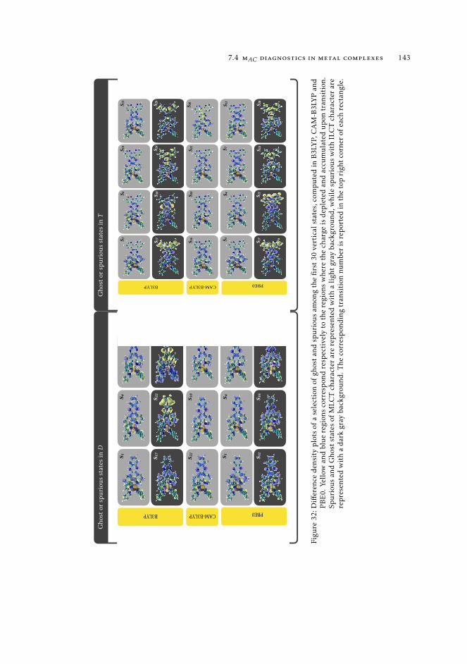
7.4 mAC diagnostics in metal complexes 143
Gho
stor
spu
riou
sst
ates
inD
S 1S 4
S 6
S 17
S 22
S 29
S 22
S 18
S 22
S 11
S 16
S 17
B3LYP CAM-B3LYP
S 1S 4
S 6
PBE0
Gho
stor
spu
riou
sst
ates
inT
S 1S 4
S 10
S 17
S 18
S 24
S 16
S 20
S 22
S 17
S 22
S 24
B3LYP CAM-B3LYP
S 1S 4
S 7
PBE0
S 13
S 29
S 28
S 11
S 30
Figu
re32
:Diff
eren
cede
nsit
ypl
ots
ofa
sele
ctio
nof
ghos
tan
dsp
urio
usam
ong
the
firs
t30
vert
ical
stat
es,c
ompu
ted
inB
3LY
P,C
AM
-B3L
YP
and
PB
E0.
Yell
owan
dbl
uere
gion
sco
rres
pond
resp
ecti
vely
toth
ere
gion
sw
here
the
char
geis
depl
eted
and
accu
mul
ated
upon
tran
siti
on.
Spur
ious
and
Gho
stst
ates
ofM
LCT
char
acte
rar
ere
pres
ente
dw
ith
ali
ght
gray
back
grou
nd,w
hile
spur
ious
wit
hIL
CT
char
acte
rar
ere
pres
ente
dw
ith
ada
rkgr
ayba
ckgr
ound
.The
corr
espo
ndin
gtr
ansi
tion
num
ber
isre
port
edin
the
top
righ
tco
rner
ofea
chre
ctan
gle.
144 mAC diagnostics in metal complexes
7.4.1 Triplet states
Although by now we have only mentioned singlet excitations, triplet excited states de-serve a mention. The role of triplet states in D and T polypyridyl complexes is crucial.Previously, it has been shown that the relative energies of the low-lying triplet states ofdifferent nature—IL(dppz,tpphz), MLCT(bpy), MLCT(Tat), and MLCT(taT) govern theluminescence properties of such class of complexes - see Appendix, Figure 55 for a thenomenclature of the fragments. This observation is due to the different sensitivity ofexcited states of different character to the substituents, and to the environment in whichthey are created.
Once again, we have used the MAC diagnostic to assess the quality of the tripletstates in complexes D and T , and to determine their character and relative abundance.Figure 33 shows the excitation energies, relaxed and unrelaxed DCT values of the lowestthirty vertical triplet states of the two complexed, calculated using B3LY. As for thesinglet excitations the excited state manifold comprises excitations of various characters.However, for both complexes, the low-energy states are no longer dominated by MLCTstates. Among the lowest states, at ≈ 2.4 eV and 2.6 eV - respectively in D and T -several ILCT transitions appear, involving both the dppz/tpphz and the bpy ligands -see Appendix, Figures 58 and 59. The MAC diagnostics allows to classify several of thetriplet states as ghosts, for instance T2 in D and T1,T5 in T . It is important to notice thatin the case of triplet states no distinction between spurious and ghost states can be made,as all vertical triplet states are dipole forbidden. This observation, however, does notmean that these states are of no interest. As already mentioned, low lying triplet stateshave been shown to be crucial in the photochemistry of such complexes [208], as they arerapidly accessed through intersystem crossing from the lowest absorbing singlet states.The presence of ghost states among the lowest triplet states suggests that one shouldproceed with all due caution, to select the correct state to optimize.
7.5 conclusions
In this last analysis we showed how the MAC diagnostics can be applied to providea detailed analysis of the excited state manifold of metal complexes. The variety oftypes of electronic transitions present in organometallic compounds makes it difficult tocharacterize them in a systematic and unambiguous manner, especially since in TDDFTthe choice of a functional can have a tremendous impact on the accuracy of the resultswhen CT states are involved. Complex photochemical processes are closely linked to thisclass of transitions and mainly develops through these.
We have characterized the transitions of four metal complexes. The first two, homolep-tic complexes, are substantially free of through-space charge-transfer states, while in theremaining two, heteroleptic complexes, the presence of a strongly conjugated polyaro-matic ligand allows the the formation of though-space transitions. As these transitionscan be delocalized across the entire length of the substituents, they are susceptible ofbeing incorrectly modeled, using the most common density functional approximation.

7.5 conclusions 145
As announced, the transitions in complexes such as [Ru(tpy)2]2+and [Ru(bpy)3]2+arefree of errors related to the presence of charge-transfer transitions. The choice of the func-tional to be used can easily be done on the basis of the maximum similarity with the experi-mental spectrum. For complexes such as [Ru(bpy)2(dppz)]2+and [Ru(bpy)2(tpphz)]2+it isnecessary to verify that no ghost states appear, which could compromise the interpretationof the photochemical behavior of the system. The diagnostic analysis revealed the almosttotal absence of ghost states among the singlet states, even when using hybrid functionalssuch as PBE0 and B3LYP. These functional also guarantee the best agreement with theexperimental data. Their use is therefore to be preferred over range separated functionals.Triplet states should be treated carefully, as one cannot distinguish between spurious statesand ghost states. By construction, triplet states have zero oscillator strength, thereforemaking it difficult to assess the margin of error associated with the calculation.
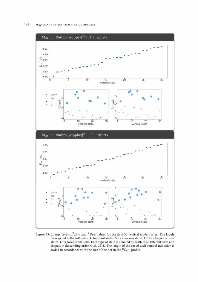
146 mAC diagnostics in metal complexes
MAC in [Ru(bpy)2(dppz)]2+- (D), triplets
0 5 10 15 20 25 30vertical state
2.25
2.50
2.75
3.00
3.25
3.50
E exc
\ eV
0 10 20 30vertical state
0
2
4
UD
CT/Å
B3LYP
flag
G
L
0 10 20 30vertical state
0
1
2
3
RD
CT/Å
MAC in [Ru(bpy)2(tpphz)]2+- (T ), triplets
0 5 10 15 20 25 30vertical state
2.50
2.75
3.00
3.25
3.50
E exc
\ eV
0 10 20 30vertical state
0
2
4
UD
CT/Å
B3LYP
flag
G
L
0 10 20 30vertical state
0
1
2
3
4
RD
CT/Å
Figure 33: Energy levels, UDCT and RDCT values for the first 30 vertical triplet states. The labelscorrespond to the following: G for ghost states, S for spurious states, CT for charge-transferstates, L for local excitations. Each type of state is denoted by scatters of different sizes andshapes, in descending order, G, S, CT, L. The length of the bar of each vertical transition isscaled in accordance with the size of the dot in the RDCT profile.

Part III
EXPLORAT ION OF THE EXC ITED STATE LANDSCAPE
ALONG A RELAXAT ION PATHWAY BASED ON THE
REORGANIZAT ION OF THE DENS ITY

8FOLLOWING EXC ITED STATES IN MOLECULAR SYSTEMS US ING
DENS ITY-BASED INDEXES
8.1 context
In the previous chapters we have extensively discussed the concept of charge-transfer,how to measure the spacial extent of a given transition, what are the challenges in suchmeasure, and how to handle them. By now, we have applied these concepts in the contextof vertical transitions, occurring between the ground state and any excited state of interest.The logical step forward is to investigate the subsequent charge-reorganization process,leading to the population of the emissive state. This observation is consistent with theintuitive picture that, after a vertical excitation, a system will tend to structurally relaxin order to minimize the produced excited state charge separation and reorganization.Here we extend the concepts introduced previously to account for excited-to-excited statetransitions. In this context, the DCT is no longer strictly related to the spatial amplitudeof the charge separation produced by ground state to excited states electronic excitation,but to the distance between two excited states.
The present chapter is inscribed in this general context. The approach that we outlinehere combines together several density descriptors, originally devised for the qualitativeinterpretation of experimentally observed phenomena, and is aimed to provide a simplephysical picture of the mechanism of excited state processes. Our strategy is intended toafford a computationally inexpensive characterization of excited state potential energysurfaces, which can be computed –on the fly- to allow both the identification of criticalareas for TDDFT approaches and the qualitative recognition –in conjunction with energycriteria- of possible reactions paths.
We introduce, in the following, a new density based index, Π, which can be used toobtain a qualitative measure of the work necessary to redistribute the electron densitygoing from one excited state to another at a given electronic configuration. Previouslyapplied to disclose non-radiative decay channels from the first excited state to the groundstate [2], this descriptor is simple, inexpensive, and can be coupled to any quantum methodable to provide a description of electronic excited states. Indeed, it relies only on theknowledge of energetics and electron densities of the different electronic states involvedin a decay. To exemplify the insights that this indexes may bring to the description excitedstate processes, we examine two distinct type of reactions. The first is an intramolecularproton transfer in occurring in CPDNO (1-(cyclopropyl)diazo-2-naphthol), an aromatic-azo compound, followed by the photo-induced charge-transfer processes in DMABN (N,N-dimethylaminobenzonitrile) and Phen-PENMe2 (5-(4-dimethylaminophenylenylethylyn)-1,10-phenanthroline). All these molecules have been previously introduced in Chapter 6,where we have checked the reliability of the TDDFT methodology applied to compute
149
150 following excited states in molecular systems using density-based indexes
their potential energy curves along specific reaction coordinates. Besides, these systemshave been extensively investigated and numerous studies exist in the literature, boththeoretical [163, 216, 217] and experimental [188, 193, 218] level. The agreement withthese earlier studies substantiates our results.
This chapter constitutes an adaptation of two previous works of myself, the first pub-lished in Journal of Computational Chemistry, in collaboration with Juan Sanz-Garcia,Marco Campetella and Ilaria Ciofini [6], the second, featured together with Anna Perfettoand Ilaria Ciofini and published in the Journal of Photochemistry and Photobiology A.
8.2 introduction
Phototriggered charge-transfer reactions typically occur through the redistribution ofthe electronic charge induced by the interaction with light. The principal actors suchprocesses, and in particular the ones we are about to describe are electrons and protons,which are transferred intramolecularly between different regions of a molecule. Thereactions we examine belong to the category of excited state intramolecular proton transfer(ESIPT) and photoinduced electron transfer reactions.
The study of excited state (ES) reaction pathways, beyond the simple analysis of verticalexcitations, far from the Franck–Condon region, is a flourishing research area [14, 19, 107,127, 128, 150, 152, 219–221]. Indeed, localizing the most stable reaction intermediates, aswell as shading light on the reaction pathways associated to photochemical processes, isstill a challenge for quantum methods nowadays available.
To gain some knowledge from theory and computational approaches on photophysicaland photochemical properties of photoactive molecules or materials is essential. Aspreviously alluded to, these are used in a wide range of applications, from optoelectronicdevices [222] to biological themes. The investigation of the mechanistic pathways thatgovern their photochemical properties is therefore essential not only for the understandingof their basic working principles but also for their design.
In this respect, it is our interest to develop simple tools to characterize the evolutionof excited state of interest along a potential energy surface (PES). However, the conceptof PESs implies that the Born–Oppenheimer approximation (BOA) holds, [27] which isgenerally true for reactions occurring at the ground state but may break down at theES [223,224]. In particular, in the case of many photoinduced processes occurring evenin simple molecular systems, for specific nuclear coordinates two or more electronic ESscan get close enough so that their coupling cannot anymore be neglected, determiningthe breakdown of the BOA [19, 27, 95]. These nuclear conformations for which the PESsof different states are very close or even cross are commonly defined as “funnel” regions,and are indeed extremely important do disclose the photochemical and photophysicalpathways of such systems. In particular, these last play a key role in defining theirnon-radiative decay pathways as well as their reactivity at the ES.
Simple approaches to identify these regions are therefore of great interest and simplifythe description of phenomena occurring at the ES tremendously. There are at least twocriteria that a method shall fulfill in order to deliver a good understanding of photochem-
8.2 introduction 151
ical processes. Firstly, it should reproduce correctly the potential energy surfaces (PES) ofthe excited states of interest, within and far from the Franck Condon (vertical excitation)region. Next, it should deliver a coherent picture of the photochemical process from theabsorption to the emission.
Ab-initio excited state dynamic approaches [225–228] can provide these informationbut are often expensive for a routine analysis. By contrast, a static study of the PES asthe one we adopt in the present chapter may provide a simplified picture of the possibledecay channels in play, delivering a realistic, yet qualitative understanding of the wholeprocess at an affordable computational cost.
Such research line is not unfrequented, and numerous theoretical studies [158, 192,229–233], including the ones previously published in my own environment, [3, 128, 159,164, 166, 216, 234] deserve a mention. As we saw in earlier chapters, the combinationof robust and reliable density functional approaches and simple descriptors based onthe electron density, provides a fair description of the PES at the excited state both froma quantitative (energy landscape) and a qualitative (hole–electron distance and chargetransfer (CT) character) point of view. [1, 3, 4]
In the preceding chapters, this type of indexes were primarily aiming at the diagnosticof TDDFT based methodologies and description of excited states with a charge-transfercharacter, with the use of the so-called DCT and MAC indexes [5]. The present discussion,instead, primarily concerns the use of density-based indexes to follow the course of thereaction induced by light, by locating and characterizing the photochemical pathways -not necessarily in terms of minimum energy paths - pursued by the molecular systemalong the potential energy surfaces (PES) of the photochemically relevant states, fromthe Franck-Condon (FC) point on the spectroscopic state to the decay to the ground statewith the formation of photoproducts. We do this based on the variation of the electrondensity distribution of the different excited states, through a recently defined index [2, 6] -so called Π - aimed at the identification of excited state potential energy regions wheredecay channels (both radiative or non-radiative) are highly expected. Unlike previousdensity descriptors, the Π index provides an estimate of the probability of differentelectronic states to interconvert, thus allowing to map the evolution of an excited statealong a reaction coordinate. The Π index can also be rationalized in terms of classicalelectromagnetism, since this density-based index can be correlated to the inverse of thework (WCT) necessary to reorganize the densities associated with two electronic ESs ofinterest.
The present chapter is thus the enforcement of the density-based approach outlinedin the beginning of this thesis, motivated by the idea of proposing a strategy to followthe evolution of excited states along a given reaction coordinate. Here, we unveil themechanistic details at work in different photochemical processes, through the Π index.We start our investigation by examining the excited state proton transfer occurring inCPDNO. Next, we analyze the ES-PESs of two dual-emissive molecules, namely DMABNand Phen-PENMe2. Their chemical structures are given in Figure 34.
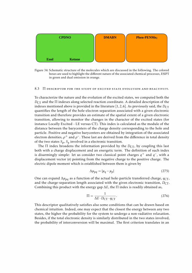
152 following excited states in molecular systems using density-based indexes
2
C6C4
C5N3N
C1
C2 C4C3 NC2
C1
N
NC2
O
N3 N4C5
H
C2C1
O
N3 N4H
Enol Ketone
CPDNO DMABN Phen-PENMe2
Figure 34: Schematic structure of the molecules which are discussed in the following. The coloredboxes are used to highlight the different nature of the associated chemical processes, ESIPTin green and dual emission in orange.
8.3 Π descriptor for the study of excited state evolution and reactivity.
To characterize the nature and the evolution of the excited states, we computed both theDCT and the Π indexes along selected reaction coordinate. A detailed description of theindexes mentioned above is provided in the literature [1,2,6]. As previously said, the DCTquantifies the length of the hole-electron separation associated with a given electronictransition and therefore provides an estimate of the spatial extent of a given electronictransition, allowing to monitor the changes in the character of the excited states (forinstance Locally Excited - LE versus CT). This index is calculated as the module of thedistance between the barycenters of the charge density corresponding to the hole andparticle. Positive and negative barycenters are obtained by integration of the associatedelectron densities, ρ+ and ρ−. These last are derived from the difference in total densityof the two states Sp, Sq involved in a electronic transition.
The Π index broadens the information provided by the DCT, by coupling this lastboth with a charge displacement and an energetic term. The definition of such indexis disarmingly simple: let us consider two classical point charges q+ and q−, with adisplacement vector (r) pointing from the negative charge to the positive charge. Theelectric dipole moment which is established between them is given by
∆µpq = |µq −µp | (275)
One can expand ∆µpq as a function of the actual hole-particle transferred charge, qCT,and the charge-separation length associated with the given electronic transition, DCT.Combining this product with the energy gap ∆E, the Π index is readily obtained as,
Π=1
∆E ·DCT · qCT. (276)
This descriptor qualitatively satisfies also some conditions that can be drawn based onchemical intuition. Indeed, one may expect that the closest the energy between any twostates, the higher the probability for the system to undergo a non-radiative relaxation.Besides, if the total electronic density is similarly distributed in the two states involved,the probability of interconversion will be maximal. The first criterion translates in an
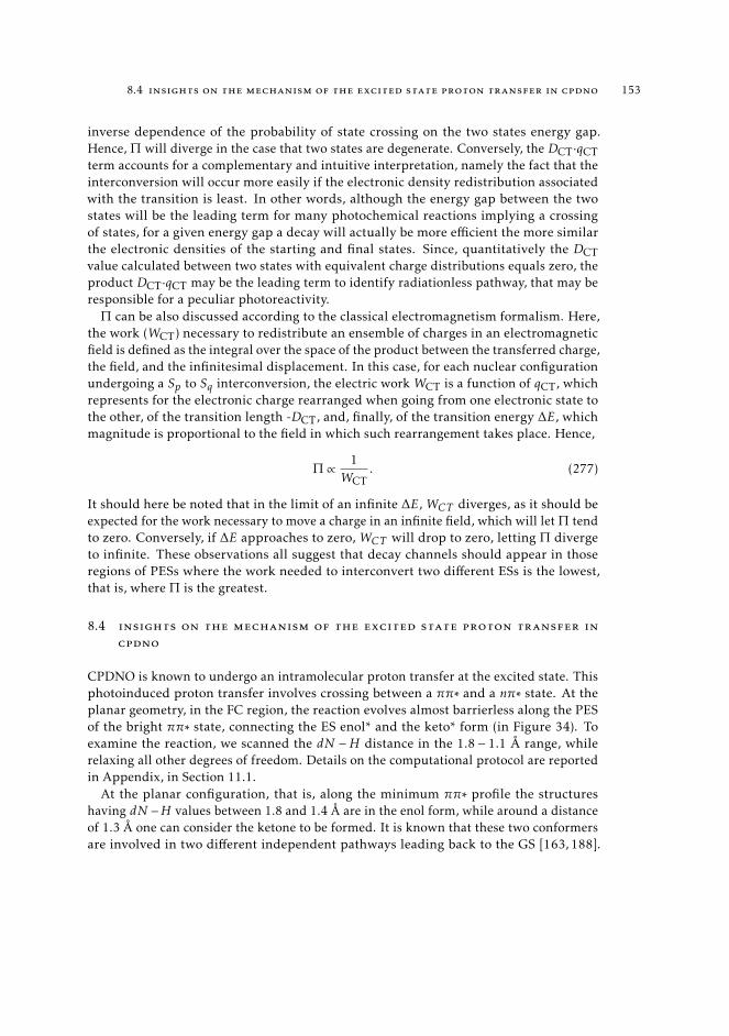
8.4 insights on the mechanism of the excited state proton transfer in cpdno 153
inverse dependence of the probability of state crossing on the two states energy gap.Hence, Π will diverge in the case that two states are degenerate. Conversely, the DCT·qCTterm accounts for a complementary and intuitive interpretation, namely the fact that theinterconversion will occur more easily if the electronic density redistribution associatedwith the transition is least. In other words, although the energy gap between the twostates will be the leading term for many photochemical reactions implying a crossingof states, for a given energy gap a decay will actually be more efficient the more similarthe electronic densities of the starting and final states. Since, quantitatively the DCTvalue calculated between two states with equivalent charge distributions equals zero, theproduct DCT·qCT may be the leading term to identify radiationless pathway, that may beresponsible for a peculiar photoreactivity.
Π can be also discussed according to the classical electromagnetism formalism. Here,the work (WCT) necessary to redistribute an ensemble of charges in an electromagneticfield is defined as the integral over the space of the product between the transferred charge,the field, and the infinitesimal displacement. In this case, for each nuclear configurationundergoing a Sp to Sq interconversion, the electric work WCT is a function of qCT, whichrepresents for the electronic charge rearranged when going from one electronic state tothe other, of the transition length -DCT, and, finally, of the transition energy ∆E, whichmagnitude is proportional to the field in which such rearrangement takes place. Hence,
Π ∝ 1WCT
. (277)
It should here be noted that in the limit of an infinite ∆E, WCT diverges, as it should beexpected for the work necessary to move a charge in an infinite field, which will let Π tendto zero. Conversely, if ∆E approaches to zero, WCT will drop to zero, letting Π divergeto infinite. These observations all suggest that decay channels should appear in thoseregions of PESs where the work needed to interconvert two different ESs is the lowest,that is, where Π is the greatest.
8.4 insights on the mechanism of the excited state proton transfer in
cpdno
CPDNO is known to undergo an intramolecular proton transfer at the excited state. Thisphotoinduced proton transfer involves crossing between a ππ∗ and a nπ∗ state. At theplanar geometry, in the FC region, the reaction evolves almost barrierless along the PESof the bright ππ∗ state, connecting the ES enol* and the keto* form (in Figure 34). Toexamine the reaction, we scanned the dN −H distance in the 1.8 − 1.1 Å range, whilerelaxing all other degrees of freedom. Details on the computational protocol are reportedin Appendix, in Section 11.1.
At the planar configuration, that is, along the minimum ππ∗ profile the structureshaving dN −H values between 1.8 and 1.4 Å are in the enol form, while around a distanceof 1.3 Å one can consider the ketone to be formed. It is known that these two conformersare involved in two different independent pathways leading back to the GS [163, 188].
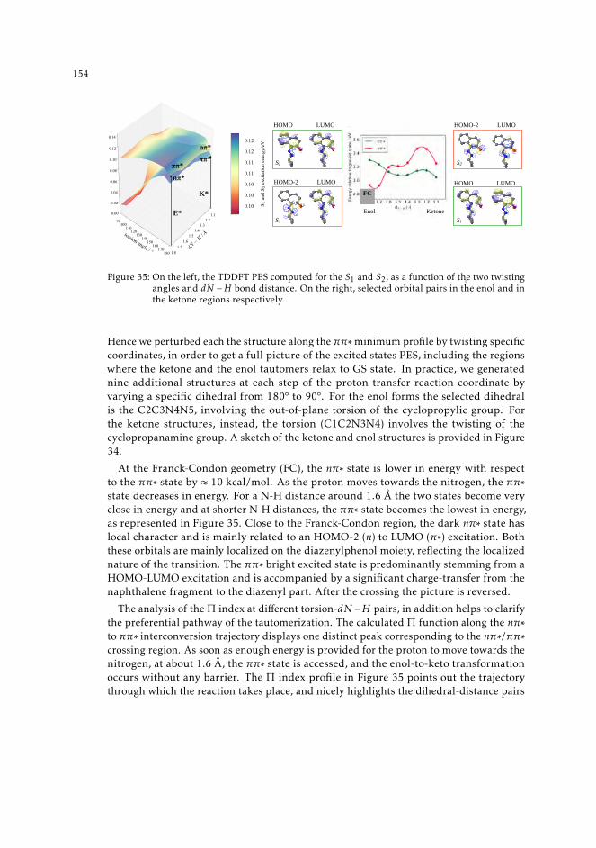
154 following excited states in molecular systems using density-based indexes
4
Ketone
HOMO-2 LUMO
Enol
S2 S2
HOMO LUMO
S1
HOMO-2 LUMO HOMO LUMO
S1
FC
E*
K*
nπ*ππ*
ππ*nπ*
Figure 35: On the left, the TDDFT PES computed for the S1 and S2, as a function of the two twistingangles and dN −H bond distance. On the right, selected orbital pairs in the enol and inthe ketone regions respectively.
Hence we perturbed each the structure along the ππ∗minimum profile by twisting specificcoordinates, in order to get a full picture of the excited states PES, including the regionswhere the ketone and the enol tautomers relax to GS state. In practice, we generatednine additional structures at each step of the proton transfer reaction coordinate byvarying a specific dihedral from 180° to 90°. For the enol forms the selected dihedralis the C2C3N4N5, involving the out-of-plane torsion of the cyclopropylic group. Forthe ketone structures, instead, the torsion (C1C2N3N4) involves the twisting of thecyclopropanamine group. A sketch of the ketone and enol structures is provided in Figure34.
At the Franck-Condon geometry (FC), the nπ∗ state is lower in energy with respectto the ππ∗ state by ≈ 10 kcal/mol. As the proton moves towards the nitrogen, the ππ∗state decreases in energy. For a N-H distance around 1.6 Å the two states become veryclose in energy and at shorter N-H distances, the ππ∗ state becomes the lowest in energy,as represented in Figure 35. Close to the Franck-Condon region, the dark nπ∗ state haslocal character and is mainly related to an HOMO-2 (n) to LUMO (π∗) excitation. Boththese orbitals are mainly localized on the diazenylphenol moiety, reflecting the localizednature of the transition. The ππ∗ bright excited state is predominantly stemming from aHOMO-LUMO excitation and is accompanied by a significant charge-transfer from thenaphthalene fragment to the diazenyl part. After the crossing the picture is reversed.
The analysis of the Π index at different torsion-dN −H pairs, in addition helps to clarifythe preferential pathway of the tautomerization. The calculated Π function along the nπ∗to ππ∗ interconversion trajectory displays one distinct peak corresponding to the nπ∗/ππ∗crossing region. As soon as enough energy is provided for the proton to move towards thenitrogen, at about 1.6 Å, the ππ∗ state is accessed, and the enol-to-keto transformationoccurs without any barrier. The Π index profile in Figure 35 points out the trajectorythrough which the reaction takes place, and nicely highlights the dihedral-distance pairs
8.5 uncovering the excited state pathway to dual emission 155
along which the reaction evolves, preferentially. Although the proton transfer occursmainly in the planar configuration, this is not the only lay in which the tautomerizationtakes place. Figure 36 well illustrates this.
The torsion of the diazenyl fragment shifts the ππ∗ state lower in energy, thus flatteningthe excited state surface. As a consequence the crossing does not necessarily occur atdN −H 1.6 but may occur at shorter distances. While at dN −H=1.6 Å the leading termis the energy, at dN −H=1.3 DCT·qCT prevails. Through the Π index, we have identifiedan additional region of the PES where the S1/S2 is efficient, which appears at shortN −H distances. Although the energy gap in this region is large, the electronic densitiesof the two states are similarly distributed. In turn, in such region, the reorganizationenergy required to interconvert the S2 ππ∗ and the nπ∗ attains a minimum, and the S1/S2transition occurs smoothly.
Identifying the existing excited state decay pathways can be of great importance, espe-cially if one wants to control a photochemical process, for example avoiding the system toevolve to a particular state, or enhancing the fluorescence from a single channel. Here,we have demonstrated how with a static approach we can identify possible non-radiativechannels - not immediately evident only on the basis of energetic arguments - based onthe similarity of the electronic density distributions of the two states. In the followingwe apply the Π index to identify the decay pathways at play in two excited state charge-transfer reactions. We aim to uncover the decay channels that contribute to populate theemitting levels.
Figure 36: Left to right: 2D map of the Π index, DCT·qCTmap and 1/∆E map, all in a.u., calculatedalong the two reaction coordinates. All quantities are computed at the PBE0/6-31G(d)level of theory.
8.5 uncovering the excited state pathway to dual emission
Dual emission in molecular systems is a phenomenon increasingly reported in the lit-erature and attracting ever-growing interest [235–239]. Depending on the mechanismat the origin of dual emission, various classes of compounds may be identified. Indeed,widely documented is dual fluorescence occurring in small organic dyes undergoingexcited state intramolecular proton-transfer (ESIPT) reactions [83, 158, 240–243] or ex-cited state intramolecular charge-transfer processes. [128, 193, 216, 230, 237, 243–246].Such dual-emission phenomena have been exploited in the synthesis of various novel
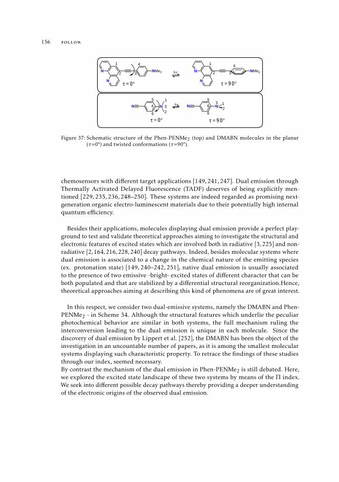
156 following excited states in molecular systems using density-based indexes
N
N
NMe2 N
N
NMe2
τ = 0° τ = 9 0°
hν
N N54
1
6
32
N N 12
354
6
hν
1
2 3
41
2 3
4
τ = 0° τ = 9 0°
Figure 37: Schematic structure of the Phen-PENMe2 (top) and DMABN molecules in the planar(τ=0°) and twisted conformations (τ=90°).
chemosensors with different target applications [149, 241, 247]. Dual emission throughThermally Activated Delayed Fluorescence (TADF) deserves of being explicitly men-tioned [229, 235, 236, 248–250]. These systems are indeed regarded as promising next-generation organic electro-luminescent materials due to their potentially high internalquantum efficiency.
Besides their applications, molecules displaying dual emission provide a perfect play-ground to test and validate theoretical approaches aiming to investigate the structural andelectronic features of excited states which are involved both in radiative [3, 225] and non-radiative [2, 164, 216, 228, 240] decay pathways. Indeed, besides molecular systems wheredual emission is associated to a change in the chemical nature of the emitting species(ex. protonation state) [149, 240–242, 251], native dual emission is usually associatedto the presence of two emissive -bright- excited states of different character that can beboth populated and that are stabilized by a differential structural reorganization.Hence,theoretical approaches aiming at describing this kind of phenomena are of great interest.
In this respect, we consider two dual-emissive systems, namely the DMABN and Phen-PENMe2 - in Scheme 34. Although the structural features which underlie the peculiarphotochemical behavior are similar in both systems, the full mechanism ruling theinterconversion leading to the dual emission is unique in each molecule. Since thediscovery of dual emission by Lippert et al. [252], the DMABN has been the object of theinvestigation in an uncountable number of papers, as it is among the smallest molecularsystems displaying such characteristic property. To retrace the findings of these studiesthrough our index, seemed necessary.By contrast the mechanism of the dual emission in Phen-PENMe2 is still debated. Here,we explored the excited state landscape of these two systems by means of the Π index.We seek into different possible decay pathways thereby providing a deeper understandingof the electronic origins of the observed dual emission.
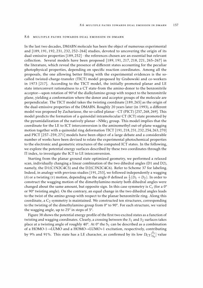
8.6 multiple paths towards dual emission in dmabn 157
8.6 multiple paths towards dual emission in dmabn
In the last two decades, DMABN molecule has been the object of numerous experimentaland [189, 191, 192, 231, 232, 252–264] studies, devoted to uncovering the origin of itsdual-emissive properties [189, 252] - the references chosen are an essential but relevantcollection. Several models have been proposed [189, 191, 217, 218, 221, 265–267] inthe literature, which reveal the presence of different states accounting for the peculiarphotophysical properties, depending on specific reaction coordinates. Among all theproposals, the one allowing better fitting with the experimental evidences is the so-called twisted-charge-transfer (TICT) model proposed by Grabowski and co-workersin 1973 [217]. According to the TICT model, the initially promoted planar and LEstate interconvert rationalness to a CT state-from the amino-donor to the benzonitrileacceptor—upon rotation of 90°of the dialkylamino group with respect to the benzonitrileplane, yielding a conformation where the donor and acceptor groups of the molecule areperpendicular. The TICT model takes the twisting coordinate [189, 265] as the origin ofthe dual-emissive properties of the DMABN. Roughly 20 years later (in 1993), a differentmodel was proposed by Zachariasse, the so-called planar - CT (PICT) [257,268,269]. Thismodel predicts the formation of a quinoidal intramolecular CT (ICT) state promoted bythe pyramidalization of the natively planar −NMe2 group. This model implies that thecoordinate for the LE to ICT interconversion is the aminomethyl out-of-plane waggingmotion together with a quinoidal ring deformation TICT [191,218,231,232,254,263,270]and PICT [257–259, 271] models have been object of a large debate and a considerablenumber of works have been devised to relate the experimental photochemical propertiesto the electronic and geometric structures of the computed ICT states. In the following,we explore the potential energy surfaces described by these two coordinates through theΠ index, to investigate the ICT to LE interconversion.
Starting from the planar ground state optimized geometry, we performed a relaxedscan, individually changing a linear combination of the two dihedral angles (D1 and D2),namely, the D1(C1N2C4C5) and the D2(C3N2C4C6). Refer to Scheme 37 for labeling.Indeed, in analogy with previous studies [191,253], we followed independently a wagging(δ) or a twisting (τ) motion, depending on the angle θ defined as 1
2 (D1 +D2). In order toconstruct the wagging motion of the dimethylamino moiety both dihedral angles werechanged about the same amount, but opposite sign. In this case symmetry is Cs (for a 0°or 90° twisting angle). On the contrary, an equal change in the two dihedral angles leadsto the twist of the amino group with respect to the planar benzonitrile ring. Along thiscoordinate, a C2 symmetry is maintained. We constructed ten structures, correspondingto the twisting of the dimethylamino group from 0° to 90°. For each structure, we variedthe wagging angle, up to 25° in steps of 5°.
Figure 38 shows the potential energy profile of the first two excited states as a function oftwisting and wagging coordinates. Clearly, a crossing between the S1 and S2 surfaces takesplace at a twisting angle of roughly 40°. At 0° the S1 can be described as a combinationof a HOMO-1→LUMO and a HOMO→LUMO+1 excitation, respectively, contributing
by 9% and 91%. This state has a LE character, as confirmed by its low DCT[S1S0] value
158 following excited states in molecular systems using density-based indexes
HOMO LUMO
HOMO LUMO+1
S1
S2
τ=0˚
HOMO LUMO+1
HOMO LUMO
S1
S2
τ=90˚
Figure 38: On the left:TDDFT PES computed for the S1 and S2, as a function of twisting and waggingangles. Top right: 2D map of the Π index, DCT·qCTmap and 1/∆E map, all in a.u.,calculated along the two reaction coordinates. All quantities are computed at the PBE0/6-31G(d) level of theory. Bottom right:selected orbital pairs in the planar and twistedconformations, respectively
of 0.87 Å. Conversely, for the same geometrical structure, S2 results essentially froma HOMO→LUMO excitation (96%) with a small percentage of a HOMO-1→LUMO+1
excitation (4%). In this case, a large DCT[S2S0] value is computed (1.81 Å) and a dipole
S0 moment by 7.5 Debye greater than the S1 dipole (4.0 Debye), both connotative of CTcharacter. As the dimethylamino group approaches the 90° twist the picture is indeedreversed, the HOMO→LUMO character changing from ππ∗ to nπ∗ (see Figure 38). Thus,for larger twisting angles, the S1 progressively changes its nature to be the CT stateobserved at planar geometry, with large CT, large polarity, and small oscillator strength,due to the poor overlap between the nitrogen lone pair orbital and the π ring.
Figure 38-(a) shows a 2D map of the Π index calculated in the space of twisting andwagging angles. A clear peak appears in correspondence of 40° twist and 0° waggingangles. This spike, by far larger than what observed for any other pair of dihedral angles,clearly indicates that the electronic distributions are most akin is at this point, providingus with an unequivocal interpretation of the crossing occurring at the same spot inthe PES. Once again, the decomposition of the Π index map endorses a step forwardin the interpretation, yielding a clear and intuitive picture of the crossing at differenttwisted/wagged geometries. Figure 38 shows the distribution of the 1/∆E function alongthe two reaction coordinates. Close to the region of δ=0° and θ=40°, the inverse of theenergy has the same behavior as the Π function, scaled by a factor of roughly a third. TheDCT·qCTdisplays a minimum in the same region. Unlike in the 1/∆E surface, this shallowregion propagates in the same range of twisting values over the whole range of waggingangles, revealing a decay pathway connecting the 0° δ - 40° τ region and the 25° δ -10° θregion.
8.7 an excursion through the excited energy levels of phen-penme2 159
We have mentioned earlier that the Π index is inversely proportional to the work thatneeds to be accomplished to rearrange two charge distributions. Hence, the maximumregion in the Π function points out the portion of the reaction space where the workneeded to reorganize the S2 into S1 (and vice-versa) is the least, and the LE to CT transitionis more likely to occur. Indeed, a large wagging motion of 25° strongly increases thepossibility of the decay to occur at small twisting angles, around 10°. However, as soon asthe twist becomes larger, the wagging motion reduces the probability of a non-radiativerelaxation and with it the likelihood of the CT state to be populated.
In agreement with previous theoretical and experimental findings, we can assert that,while the twisting coordinate remains predominant, the wagging motion contributes toconvey the system toward in the ICT state (where the emission occurs). In summary, theΠ index individuates the S1/S2 crossing at the correct position, and more importantly ithelps to identify other non-radiative decay channels, highlighting the role of the inversionmode on the ICT process in a simple and unequivocal manner.
8.7 an excursion through the excited energy levels of phen-penme2
Phen-PENMe2 can be considered as a typical push-pull system thus similar to manydual-emissive molecules relying on a Donor-π bridge-Acceptor structure (D-π-A). It iscomposed of a 1,10-phenanthroline core functionalized with a dimethylaminophenylgroup acting as an electron donor, as shown in Figure 37. Recent combined experimentaland theoretical studies performed by some of us [193,216] clarified that the observed dualemission is associated with the existence of two different emissive states: a planar Intra-Molecular Charge Transfer (ICT) state corresponding to an electronic transition from thedonor moiety to the phenanthroline core, and a Locally Excited (LE) - state centered on the1,10-phenanthroline, in which the donor and acceptor are orthogonally oriented. Theseearlier experimental and theoretical studies also investigated the solvent dependence ofthe dual-emission phenomenon and highlighted the importance of the use of polar-aproticsolution to allow for the formation of both conformations, thus yielding the dual emission.If the nature of the emissive states has been disclosed, [216] the pathways connectingthe excited states initially populated in absorption to the ones that actually emit has notyet been thoroughly analyzed. This is the question we aim to answer in this work, usingdensity-based descriptors.
8.7.1 Considerations on the energy profiles of the lowest excited states.
To investigate the photophysical behavior of the Phen-PENMe2 molecule we analyze theevolution of the ground state and of the first six excited states, along the coordinate ofinterest (in Scheme 37). This last involves the formation of a planar and an orthogonalconformer, which differ in the orientation of phenyl and phenanthroline rings. Groundstate DFT calculations computed at each reaction step revealed a rather flat ground statepotential curve. The planar structure (τ=0°) is the minimum, though only by 0.04 eV
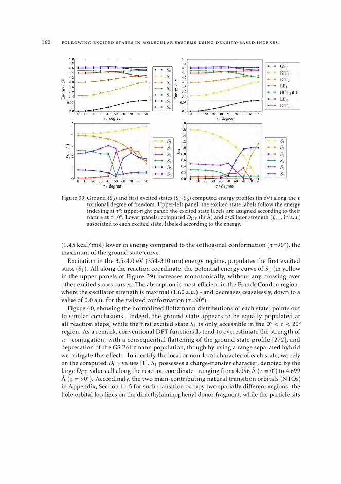
160 following excited states in molecular systems using density-based indexes
Figure 39: Ground (S0) and first excited states (S1-S6) computed energy profiles (in eV) along the τtorsional degree of freedom. Upper-left panel: the excited state labels follow the energyindexing at τ°; upper-right panel: the excited state labels are assigned according to theirnature at τ=0°. Lower panels: computed DCT (in Å) and oscillator strength (fosc, in a.u.)associated to each excited state, labeled according to the energy.
(1.45 kcal/mol) lower in energy compared to the orthogonal conformation (τ=90°), themaximum of the ground state curve.
Excitation in the 3.5-4.0 eV (354-310 nm) energy regime, populates the first excitedstate (S1). All along the reaction coordinate, the potential energy curve of S1 (in yellowin the upper panels of Figure 39) increases monotonically, without any crossing overother excited states curves. The absorption is most efficient in the Franck-Condon region -where the oscillator strength is maximal (1.60 a.u.) - and decreases ceaselessly, down to avalue of 0.0 a.u. for the twisted conformation (τ=90°).
Figure 40, showing the normalized Boltzmann distributions of each state, points outto similar conclusions. Indeed, the ground state appears to be equally populated atall reaction steps, while the first excited state S1 is only accessible in the 0° < τ < 20°region. As a remark, conventional DFT functionals tend to overestimate the strength ofπ - conjugation, with a consequential flattening of the ground state profile [272], anddeprecation of the GS Boltzmann population, though by using a range separated hybridwe mitigate this effect. To identify the local or non-local character of each state, we relyon the computed DCT values [1]. S1 possesses a charge-transfer character, denoted by thelarge DCT values all along the reaction coordinate - ranging from 4.096 Å (τ = 0°) to 4.699Å (τ = 90°). Accordingly, the two main-contributing natural transition orbitals (NTOs)in Appendix, Section 11.5 for such transition occupy two spatially different regions: thehole-orbital localizes on the dimethylaminophenyl donor fragment, while the particle sits
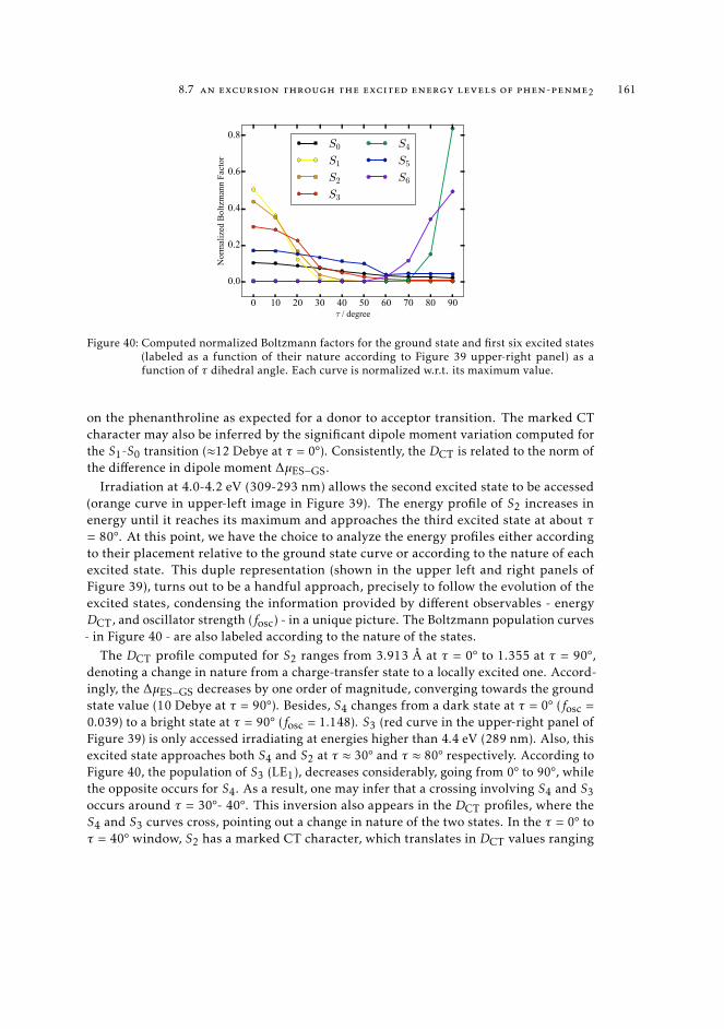
8.7 an excursion through the excited energy levels of phen-penme2 161
0 10 20 30 40 50 60 70 80 90τ / degree
0.0
0.2
0.4
0.6
0.8
Nor
mal
ized
Bol
tzm
ann
Fact
or
S0
S1
S2
S3
S4
S5
S6
Figure 40: Computed normalized Boltzmann factors for the ground state and first six excited states(labeled as a function of their nature according to Figure 39 upper-right panel) as afunction of τ dihedral angle. Each curve is normalized w.r.t. its maximum value.
on the phenanthroline as expected for a donor to acceptor transition. The marked CTcharacter may also be inferred by the significant dipole moment variation computed forthe S1-S0 transition (≈12 Debye at τ = 0°). Consistently, the DCT is related to the norm ofthe difference in dipole moment ∆µES−GS.
Irradiation at 4.0-4.2 eV (309-293 nm) allows the second excited state to be accessed(orange curve in upper-left image in Figure 39). The energy profile of S2 increases inenergy until it reaches its maximum and approaches the third excited state at about τ= 80°. At this point, we have the choice to analyze the energy profiles either accordingto their placement relative to the ground state curve or according to the nature of eachexcited state. This duple representation (shown in the upper left and right panels ofFigure 39), turns out to be a handful approach, precisely to follow the evolution of theexcited states, condensing the information provided by different observables - energyDCT, and oscillator strength (fosc) - in a unique picture. The Boltzmann population curves- in Figure 40 - are also labeled according to the nature of the states.
The DCT profile computed for S2 ranges from 3.913 Å at τ = 0° to 1.355 at τ = 90°,denoting a change in nature from a charge-transfer state to a locally excited one. Accord-ingly, the ∆µES−GS decreases by one order of magnitude, converging towards the groundstate value (10 Debye at τ = 90°). Besides, S4 changes from a dark state at τ = 0° (fosc =0.039) to a bright state at τ = 90° (fosc = 1.148). S3 (red curve in the upper-right panel ofFigure 39) is only accessed irradiating at energies higher than 4.4 eV (289 nm). Also, thisexcited state approaches both S4 and S2 at τ ≈ 30° and τ ≈ 80° respectively. According toFigure 40, the population of S3 (LE1), decreases considerably, going from 0° to 90°, whilethe opposite occurs for S4. As a result, one may infer that a crossing involving S4 and S3occurs around τ = 30°- 40°. This inversion also appears in the DCT profiles, where theS4 and S3 curves cross, pointing out a change in nature of the two states. In the τ = 0° toτ = 40° window, S2 has a marked CT character, which translates in DCT values ranging
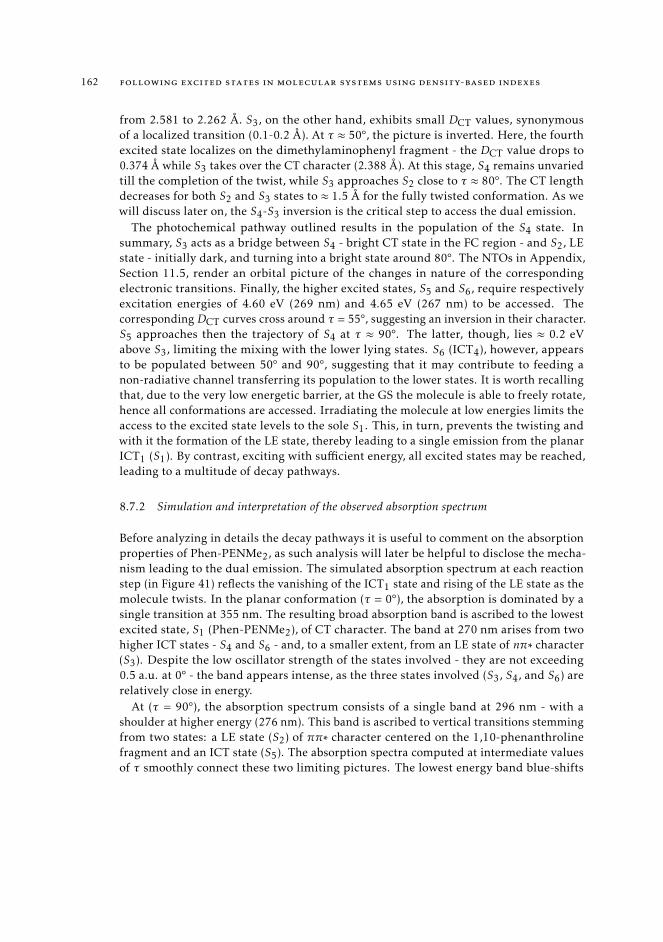
162 following excited states in molecular systems using density-based indexes
from 2.581 to 2.262 Å. S3, on the other hand, exhibits small DCT values, synonymousof a localized transition (0.1-0.2 Å). At τ ≈ 50°, the picture is inverted. Here, the fourthexcited state localizes on the dimethylaminophenyl fragment - the DCT value drops to0.374 Å while S3 takes over the CT character (2.388 Å). At this stage, S4 remains unvariedtill the completion of the twist, while S3 approaches S2 close to τ ≈ 80°. The CT lengthdecreases for both S2 and S3 states to ≈ 1.5 Å for the fully twisted conformation. As wewill discuss later on, the S4-S3 inversion is the critical step to access the dual emission.
The photochemical pathway outlined results in the population of the S4 state. Insummary, S3 acts as a bridge between S4 - bright CT state in the FC region - and S2, LEstate - initially dark, and turning into a bright state around 80°. The NTOs in Appendix,Section 11.5, render an orbital picture of the changes in nature of the correspondingelectronic transitions. Finally, the higher excited states, S5 and S6, require respectivelyexcitation energies of 4.60 eV (269 nm) and 4.65 eV (267 nm) to be accessed. Thecorresponding DCT curves cross around τ = 55°, suggesting an inversion in their character.S5 approaches then the trajectory of S4 at τ ≈ 90°. The latter, though, lies ≈ 0.2 eVabove S3, limiting the mixing with the lower lying states. S6 (ICT4), however, appearsto be populated between 50° and 90°, suggesting that it may contribute to feeding anon-radiative channel transferring its population to the lower states. It is worth recallingthat, due to the very low energetic barrier, at the GS the molecule is able to freely rotate,hence all conformations are accessed. Irradiating the molecule at low energies limits theaccess to the excited state levels to the sole S1. This, in turn, prevents the twisting andwith it the formation of the LE state, thereby leading to a single emission from the planarICT1 (S1). By contrast, exciting with sufficient energy, all excited states may be reached,leading to a multitude of decay pathways.
8.7.2 Simulation and interpretation of the observed absorption spectrum
Before analyzing in details the decay pathways it is useful to comment on the absorptionproperties of Phen-PENMe2, as such analysis will later be helpful to disclose the mecha-nism leading to the dual emission. The simulated absorption spectrum at each reactionstep (in Figure 41) reflects the vanishing of the ICT1 state and rising of the LE state as themolecule twists. In the planar conformation (τ = 0°), the absorption is dominated by asingle transition at 355 nm. The resulting broad absorption band is ascribed to the lowestexcited state, S1 (Phen-PENMe2), of CT character. The band at 270 nm arises from twohigher ICT states - S4 and S6 - and, to a smaller extent, from an LE state of nπ∗ character(S3). Despite the low oscillator strength of the states involved - they are not exceeding0.5 a.u. at 0° - the band appears intense, as the three states involved (S3, S4, and S6) arerelatively close in energy.
At (τ = 90°), the absorption spectrum consists of a single band at 296 nm - with ashoulder at higher energy (276 nm). This band is ascribed to vertical transitions stemmingfrom two states: a LE state (S2) of ππ∗ character centered on the 1,10-phenanthrolinefragment and an ICT state (S5). The absorption spectra computed at intermediate valuesof τ smoothly connect these two limiting pictures. The lowest energy band blue-shifts
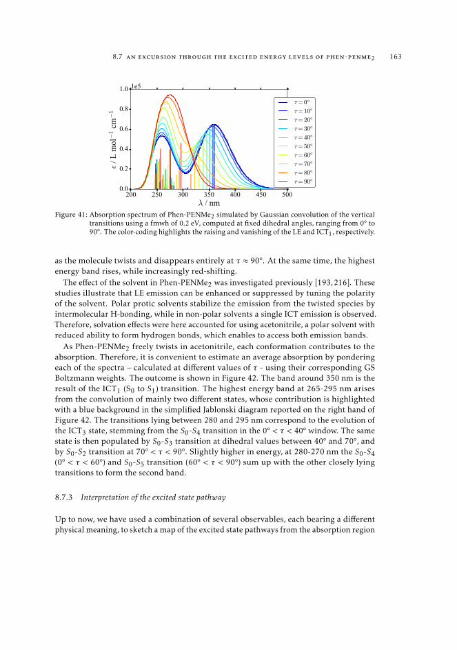
8.7 an excursion through the excited energy levels of phen-penme2 163
200 250 300 350 400 450 500λ / nm
0.0
0.2
0.4
0.6
0.8
1.0
ε / L
mol−
1 c
m−
1
1e5
τ= 0°τ= 10°τ= 20°τ= 30°τ= 40°τ= 50°τ= 60°τ= 70°τ= 80°τ= 90°
Figure 41: Absorption spectrum of Phen-PENMe2 simulated by Gaussian convolution of the verticaltransitions using a fmwh of 0.2 eV, computed at fixed dihedral angles, ranging from 0° to90°. The color-coding highlights the raising and vanishing of the LE and ICT1, respectively.
as the molecule twists and disappears entirely at τ ≈ 90°. At the same time, the highestenergy band rises, while increasingly red-shifting.
The effect of the solvent in Phen-PENMe2 was investigated previously [193,216]. Thesestudies illustrate that LE emission can be enhanced or suppressed by tuning the polarityof the solvent. Polar protic solvents stabilize the emission from the twisted species byintermolecular H-bonding, while in non-polar solvents a single ICT emission is observed.Therefore, solvation effects were here accounted for using acetonitrile, a polar solvent withreduced ability to form hydrogen bonds, which enables to access both emission bands.
As Phen-PENMe2 freely twists in acetonitrile, each conformation contributes to theabsorption. Therefore, it is convenient to estimate an average absorption by ponderingeach of the spectra – calculated at different values of τ - using their corresponding GSBoltzmann weights. The outcome is shown in Figure 42. The band around 350 nm is theresult of the ICT1 (S0 to S1) transition. The highest energy band at 265-295 nm arisesfrom the convolution of mainly two different states, whose contribution is highlightedwith a blue background in the simplified Jablonski diagram reported on the right hand ofFigure 42. The transitions lying between 280 and 295 nm correspond to the evolution ofthe ICT3 state, stemming from the S0-S4 transition in the 0° < τ < 40° window. The samestate is then populated by S0-S3 transition at dihedral values between 40° and 70°, andby S0-S2 transition at 70° < τ < 90°. Slightly higher in energy, at 280-270 nm the S0-S4(0° < τ < 60°) and S0-S5 transition (60° < τ < 90°) sum up with the other closely lyingtransitions to form the second band.
8.7.3 Interpretation of the excited state pathway
Up to now, we have used a combination of several observables, each bearing a differentphysical meaning, to sketch a map of the excited state pathways from the absorption region
164 following excited states in molecular systems using density-based indexes
GS
ICT1
ICT2
ICT4
LE1LE1
LE1
ICT3
LE2 LE2
LE
Figure 42: Left: Boltzmann weighted simulated absorption spectra of Phen-PENMe2. Right: Jablonskidiagram describing the absorption phenomena occurring in the Phen-PENMe2 molecule.
to the emitting one. Also, we have postulated the existence of several decay channels.However, to reach the correct interpretation, it is essential to assess the relative importanceof each. The Π index, precisely addresses this question. It is important to mention thoughthat the methodology we are about to discuss is based on static considerations. Therefore,it does not give any indication on the time-scale of the photochemical process. As a result,any consideration on the kinetics of the electronic process remains out of our scope.
As previously mentioned, the Π index combines energetic arguments - ∆E - and ameasure for charge rearrangement - DCT·qCT - and can be used as criteria to detect thepresence of non-radiative decay channels. It is useful to compare the relative value of theΠ between electronic transitions that involve a common electronic state. This approachprovides a reasonable estimate of the relative likelihood of a decay channel, connectingmore efficiently an electronic state with one or another state, lower in energy. Intuitively,this information shall be coupled with the vertical absorption spectra, in order to mapthe excited states all through the pathway that brings to the emission. As for this aspect,a radiative relaxation yielding an emission from any excited state Sq necessarily impliesthat this particular state of interest is populated either directly, by irradiation, or by decayfrom an energetically higher excited state. The Π index, combined with the absorptiondata, allows to estimate the relative efficiency of the relaxation pathways connectingany two states all along a reaction coordinate. The result is a qualitative strategy, whichdelivers a consonant interpretation of a photochemical process, in an uncomplicatedmanner. Besides, the Π index is also computationally inexpensive, which is often not thecase when one uses alternative approaches to deal with such questions. Undoubtedly, theglobal understanding of the physical phenomena will strongly depend on the quality ofthe ground, and excited states computed PES and thus will be affected by the level oftheory (method and basis set) used to calculate densities and energies. This said, the levelof theory which we have used to perform our calculations was proven to be well accurate -as discussed in Chapter 6. Besides, the results of a previous benchmark [128] attest a good
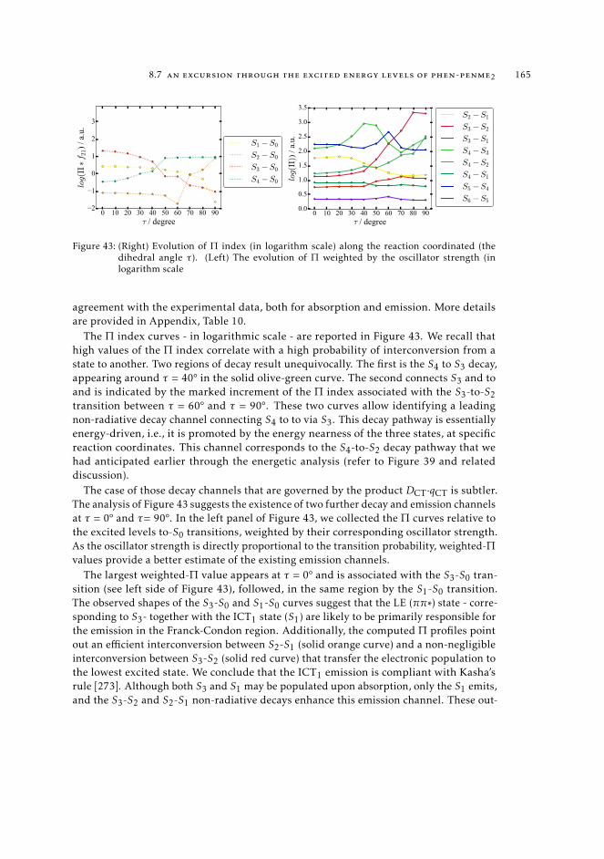
8.7 an excursion through the excited energy levels of phen-penme2 165
Figure 43: (Right) Evolution of Π index (in logarithm scale) along the reaction coordinated (thedihedral angle τ). (Left) The evolution of Π weighted by the oscillator strength (inlogarithm scale
agreement with the experimental data, both for absorption and emission. More detailsare provided in Appendix, Table 10.
The Π index curves - in logarithmic scale - are reported in Figure 43. We recall thathigh values of the Π index correlate with a high probability of interconversion from astate to another. Two regions of decay result unequivocally. The first is the S4 to S3 decay,appearing around τ = 40° in the solid olive-green curve. The second connects S3 and toand is indicated by the marked increment of the Π index associated with the S3-to-S2transition between τ = 60° and τ = 90°. These two curves allow identifying a leadingnon-radiative decay channel connecting S4 to to via S3. This decay pathway is essentiallyenergy-driven, i.e., it is promoted by the energy nearness of the three states, at specificreaction coordinates. This channel corresponds to the S4-to-S2 decay pathway that wehad anticipated earlier through the energetic analysis (refer to Figure 39 and relateddiscussion).
The case of those decay channels that are governed by the product DCT·qCT is subtler.The analysis of Figure 43 suggests the existence of two further decay and emission channelsat τ = 0° and τ= 90°. In the left panel of Figure 43, we collected the Π curves relative tothe excited levels to-S0 transitions, weighted by their corresponding oscillator strength.As the oscillator strength is directly proportional to the transition probability, weighted-Πvalues provide a better estimate of the existing emission channels.
The largest weighted-Π value appears at τ = 0° and is associated with the S3-S0 tran-sition (see left side of Figure 43), followed, in the same region by the S1-S0 transition.The observed shapes of the S3-S0 and S1-S0 curves suggest that the LE (ππ∗) state - corre-sponding to S3- together with the ICT1 state (S1) are likely to be primarily responsible forthe emission in the Franck-Condon region. Additionally, the computed Π profiles pointout an efficient interconversion between S2-S1 (solid orange curve) and a non-negligibleinterconversion between S3-S2 (solid red curve) that transfer the electronic population tothe lowest excited state. We conclude that the ICT1 emission is compliant with Kasha’srule [273]. Although both S3 and S1 may be populated upon absorption, only the S1 emits,and the S3-S2 and S2-S1 non-radiative decays enhance this emission channel. These out-
166 following excited states in molecular systems using density-based indexes
comes agree with the experimental data substantiating the existence of an efficient ICT1radiative channel [193, 216]. The vertical deactivation pathway transferring the electronicpopulation from S4 to S1 (through the S3-S2-S1 decay channels) and leading to the ICT1emission, is poorly efficient compared to the relaxation pathway activated by the torsion.As anticipated earlier in the discussion, if the molecule is irradiated with sufficiently highenergy one activates the structural relaxation, which leads to the formation of the S2 (LE)state at 90°. The pathway involves the conversion between state S4 to state S3 (at around50°) followed by the conversion of S3 to S2 at ≈ 80°.
Furthermore, as the twist approaches 90°, two channels establish, which transfer theelectronic population from S4 to S2. By contrast, the oscillator strength of S4 (0.09 a.u. inthe twisted region) is connotative of a poor absorption, suggesting that the existence of anemissive path from S4 is conditioned to the presence of a higher excited state, transferringits population to S4 through a non-radiative channel. The steep increase of the Π indexassociated with the S5 to S4 decay at τ = 90° validates this hypothesis. Similar reasoningholds for S5, whose population is maintained by S6, which absorbs at 0° and approachesS5 at 60°.
Close to τ = 90°, all Π curves, except that computed for the S3-S1, S2-S1, and the S1-S0interconversion visibly rise. This pattern suggests the existence of several interconnecteddecay-channels (S4-S3, S4-S2, S3-S2), which transfer the population from S4 to S2. Oncemore, these sub-channels are not necessarily driven by the energy gap, which rangesbetween 0.01 a.u. for S4-S2 and 0.003 a.u. for S3-S2. As such, the formation of thesechannels is supported by the similar distributions of the electronic densities of the statesinvolved, as witnessed by the small DCT·qCT values - computed Π values are reportedin Table 17. Remarkably, the drop in the S1-S0 weighted-Π curve suggests the absenceof the emission from S1 (ICT1) at 90°. Indeed, the orthogonality of the donor (dimethy-laminophenyl) and acceptor (1,10-phenanthroline) hinders the formation of the ICT1state. As a consequence, the lowest emitting state at τ = 90° is S2 (LE).
In light of the discussion above, the dual emission mechanism observed in Phen-PENMe2 can be summarized by the Jablonski diagram shown in Figure 44. The populationof the S1 - ICT1 planar state in the FC region - leads to the ICT1 emission, calculatedat 560 nm. Moreover, irradiation at a higher excitation wavelength allows reaching S4.From S4 a decay channel can open, leading to the population of to S2, a ππ∗ state of localcharacter (LE). The relaxation through the vibrational sub-levels of S2 causes the observedfluorescence band (at 421 nm).
The S4-S0 curve suggests the existence of a further radiative decay at τ = 90 °. Thischannel is connected to S6 - in the planar conformation. However, further internaldeactivation channels between S4-S3 and S3-S2 can intervene, reducing the decay fromS4 and resulting in an enhanced S2-S0 emission. Similarly, S3-S1 and S3-S2 curves hint tothe existence of two non-radiative channels which, in the planar conformation, contributeto impoverish the S3-S0 channel. These evidences, altogether, suggest that the emissionfrom the LE state violates Kasha’s rule. To explain this unusual behavior, it is instructiveto examine the energy, and DCT·qCT values of the S2-S1 transition, at τ = 0 ° and τ = 90 °.At τ = 0° ∆E equals 0.021 a.u.. The DCT·qCT product is small (0.83 a.u.), which reflects
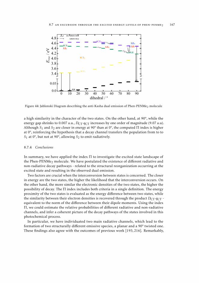
8.7 an excursion through the excited energy levels of phen-penme2 167
GS
ICT1
ICT2
ICT4
LE1 LE1LE1
ICT3LE2
LE
non- radiative decay
radiative decay
Figure 44: Jablonski Diagram describing the anti-Kasha dual emission of Phen-PENMe2 molecule
a high similarity in the character of the two states. On the other hand, at 90°, while theenergy gap shrinks to 0.007 a.u., DCT·qCT increases by one order of magnitude (9.07 a.u).Although S1 and S2 are closer in energy at 90° than at 0°, the computed Π index is higherat 0°, reinforcing the hypothesis that a decay channel transfers the population from to toS1 at 0°, but not at 90°, allowing S2 to emit radiatively.
8.7.4 Conclusions
In summary, we have applied the index Π to investigate the excited state landscape ofthe Phen-PENMe2 molecule. We have postulated the existence of different radiative andnon-radiative decay pathways - related to the structural reorganization occurring at theexcited state and resulting in the observed dual emission.
Two factors are crucial when the interconversion between states is concerned. The closerin energy are the two states, the higher the likelihood that the interconversion occurs. Onthe other hand, the more similar the electronic densities of the two states, the higher thepossibility of decay. The Π index includes both criteria in a single definition. The energyproximity of the two states is evaluated as the energy difference between two states, whilethe similarity between their electron densities is recovered through the product DCT·qCT -equivalent to the norm of the difference between their dipole moments. Using the indexΠ, we could estimate the relative probabilities of different radiative and non-radiativechannels, and infer a coherent picture of the decay pathways of the states involved in thisphotochemical process.
In particular, we have individuated two main radiative channels, which lead to theformation of two structurally different emissive species, a planar and a 90° twisted one.These findings also agree with the outcomes of previous work [193, 216]. Remarkably,

168 following excited states in molecular systems using density-based indexes
our analysis points out the anti-Kasha mechanism of the LE emission. Besides, we haveidentified several sub-channels that play an essential role, enhancing either of the twoemissions. To conclude, the analysis that we have carried out shows the capability of theΠ index to draw a qualitative map of a photochemical reaction.
9A STATE - SPEC I F IC F INGERPR INT FOR AN EFF IC IENT EXC ITED
STATE TRACKING
9.1 context
Tracking each excited state along a reaction coordinate is a crucial problem in photo-chemistry. While calculating the optical properties is certainly a start, absorption andemission spectra do not provide any information on the path that each state traversesin the excited state, and it can be complicated to draw the connection between energyabsorption and photoproducts formation. Topological descriptors can be very useful tocharacterize the nature of an excited state. In particular, they conveniently translate theinformation contained in mathematical objects, such as the 1DDM [115], into a morecompact and readable representation of the electronic transition, and can, therefore, beuseful to examine the nature of an excited state along a reaction coordinate. Still, fullyunderstanding where among all vertical positions to find a state of interest, and mappingthe position of one particular excited state at successive points of a reaction coordinate,remains a non-trivial task that is, nevertheless, indispensable to assemble a coherentdescription of a reaction pathway [151].
This problem forms the central task of this chapter. Here, we propose a new rigorousmetric to track excited states along a reaction coordinate, based on the DCT density-baseddescriptor. The DCT translates the information contained in the densities of the initial andfinal states into a length and provides a simple measure of the spatial extent of an elec-tronic transition. We have used this approach repeatedly in the previous chapters, wherewe have characterized the nature of excited states all along specific reaction coordinatesthrough their DCT values - calculated with respect to their corresponding ground statedensity distribution at same geometry. Although the DCT is specific for a given transition,it is not sufficient to characterize a state uniquely among a set of vertical excited states. Infact, there may be several close-lying states with similar character, whose ambiguity mayprevent the precise identification of a state of interest along a reaction coordinate.
We attempt to solve this indefiniteness with a new metric, which delivers a uniquerepresentation of the excited state. Instead of characterizing a vertical state in termsof a one-electron transition from the ground state, we use the collection of DCT vectorscalculated between that state and any other state, at same geometry. In other words, wecharacterize each state by encrypting its connotations in a state-specific "fingerprint."Then, we compare each pair of states using a purposely-defined geometrical distancebetween their corresponding fingerprints.
We have implemented such a metric in a simple algorithm to map the evolution ofexcited states along a reaction coordinate. The algorithm determines the relative arrange-ment of a set of vertical states by computing the distance between the fingerprints of each
169
170 a state-specific fingerprint for an efficient excited state tracking
pair of states at successive steps and selecting the one that minimizes all distances. Weevaluate the performance of this reaction-map-search by comparing the results with areference representation, where we estimate the similarity between all pairs of states byvisually inspecting the main-contributing orbitals and the relevant density descriptors.Additionally, we discuss a possible alternative to the fingerprint-method, consisting inevaluating the distance between each pair of states through the overlap of the correspond-ing wavefunctions.
9.2 introduction
From small compounds to transition metal complexes, the presence of electron donatingand accepting groups gives rise to a rich variety of excited states, either localized orextended on more functional groups, which are responsible for the photophysical andphotochemical properties of each system.
Tracking each excited state along a reaction coordinate is a crucial problem in photo-chemistry. Indeed, solving the "tracking problem” is the starting point to address detailedchemical questions, such as following excited state pathways and understanding how andwhere photoproducts are formed along the reaction path.
Not surprisingly, this problem has attracted a broad interest in the recent literatureand several solutions have been proposed, for example, in the framework of vibrationalquantum dynamics of molecules in different environments and in experimental andcomputational studies of organic and inorganic photochemistry [14,274–278]. For whatconcerns theoretical approaches, a standard procedure is to identify the excited states byconsidering the most important excitation coefficients of the wave function and visuallyinspecting the corresponding orbitals [220, 231, 255, 278, 279], and more often naturaltransition orbitals [24,92,107,202,205,206]. However, this procedure is often tedious andimprecise, as it relies on subjective inspection of the orbitals involved in the excitation.Therefore, it is desirable to devise more automatic and quantitative techniques for excitedstate characterization. Some attempts have been proposed in the recent literature, forexample based on quantitative analysis of the wavefunction contributions through theiroverlaps [109, 280–282], but a general and standardized approach to this problem is, atthe present day, still lacking.
In the previous chapter, we have shown that one can determine the relative importanceof different decay pathways by using the Π index [7]. Such analysis was proven tobe helpful to identify the pathway that interconnects excited states along a reactioncoordinate. However, ambiguities might arise as it is not always easy to map the excitedstates in an unequivocal manner.
This chapter proposes a novel approach to the problem of following the evolution ofdifferent excited states along a reaction coordinate. Our aim is to establish a methodologyto map the vertical position of any excited state along a reaction coordinate from theinitial configuration - usually in the Franck-Condon region - up to a designated finalconformation. In other words, we search for the position of each state, at different steps ofreaction, relative to a reference distribution of vertical excited states at the initial step.
9.3 methods 171
This question is unavoidably related to our capability of monitoring the character ofthe involved excited states, which, as pointed out throughout this thesis, collectivelydetermine the photophysics and photo-chemistry of molecular systems.
In the previous chapters we have introduced and applied several descriptors for thecharacterization of excited states: The DCT quantifies the global density redistributionupon excitation, and measures the charge-transfer character - i.e. the spacial amplitude ofthe charge separation produced by an electronic excitation. Another observable that weused is the qCT i.e., the integrated charge transferred upon transition. Aside to these, theoscillator strength, denoted as fosc is also significant, as it measures the efficiency withwhich a particular transition couples to the light at that frequency. Finally, a quantity thatis clearly of primary importance is the energy of the excited state, it determines how statesare distributed one respect to the other. In this regard, we remind that a small energygap between two states increases the probability of transition [14, 151, 224]. Although allof these observables singularly account for a different aspect of an electronic transition,it is not always easy to combine them to achieve an unambiguous interpretation of theexcitation process.
As we have previously shown, the DCT vector to the ground state is a powerful descrip-tor for the state character. Moreover, it is easy to interpret this quantity as a displacementvector in the 3-dimensional space. Here, we extend this descriptor by considering, at thesame time, the whole set of DCT vectors from the state under consideration to all the otherexcited states at the same geometry. The idea is to use the geometrical properties of thiscollection of vectors as a "fingerprint" for the character of the excited state.
9.3 methods
9.3.1 State tracking procedure
We aim to track the reaction path of a set of vertically-excited states distributed along areaction coordinate.
Definition 1 We define S as the matrix of the excited states along the reaction coordinate,where St,i is the excited state that has vertical index i at reaction coordinate t.
Definition 2 We define the "follow index" FFF as the map of all state pathways along thereaction coordinate, where Ft,i is the vertical index, evolved at reaction coordinate t, of S(0, i).
In other words, Ft,i tells where, among the vertical positions, one can find the excited statethat was at position i at the zero reaction coordinate. The latter implies that F (0, i) = i.The goal of our computational protocol is to find the FFF that better approximates the truematrix FFF T , defined as the follow index as inferred by orbital and descriptors analysis bya human.
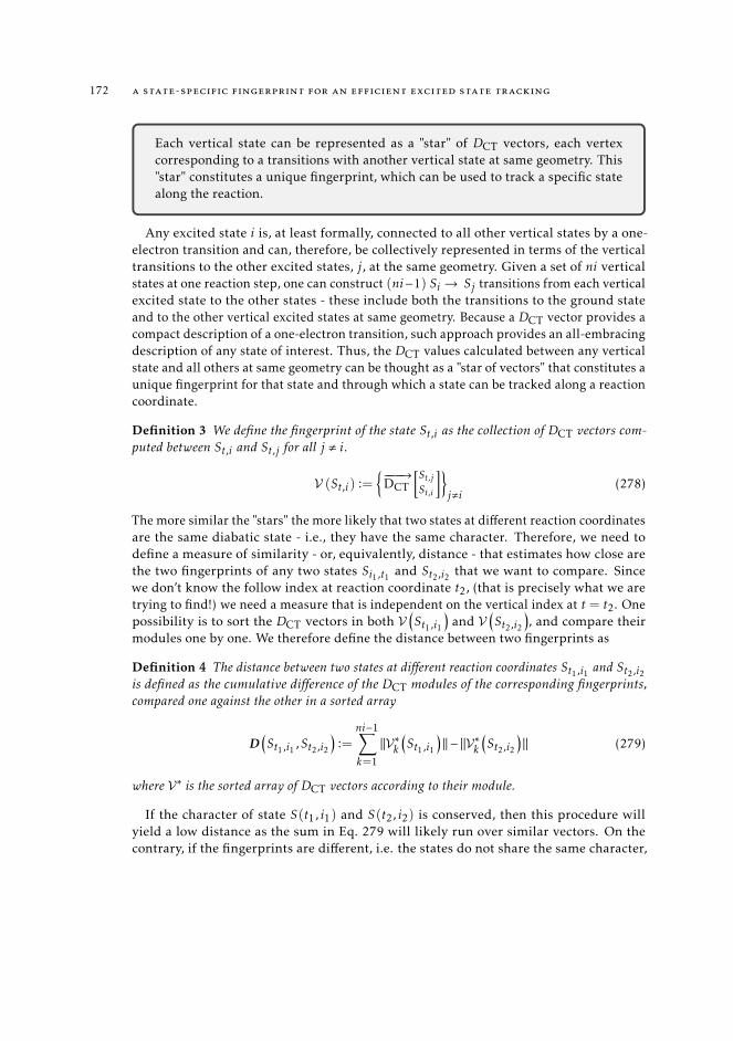
172 a state-specific fingerprint for an efficient excited state tracking
Each vertical state can be represented as a "star" of DCT vectors, each vertexcorresponding to a transitions with another vertical state at same geometry. This"star" constitutes a unique fingerprint, which can be used to track a specific statealong the reaction.
Any excited state i is, at least formally, connected to all other vertical states by a one-electron transition and can, therefore, be collectively represented in terms of the verticaltransitions to the other excited states, j, at the same geometry. Given a set of ni verticalstates at one reaction step, one can construct (ni−1) Si → Sj transitions from each verticalexcited state to the other states - these include both the transitions to the ground stateand to the other vertical excited states at same geometry. Because a DCT vector provides acompact description of a one-electron transition, such approach provides an all-embracingdescription of any state of interest. Thus, the DCT values calculated between any verticalstate and all others at same geometry can be thought as a "star of vectors" that constitutes aunique fingerprint for that state and through which a state can be tracked along a reactioncoordinate.
Definition 3 We define the fingerprint of the state St,i as the collection of DCT vectors com-puted between St,i and St,j for all j , i.
V (St,i) :=−−−−→
DCT
[St,jSt,i
]j,i
(278)
The more similar the "stars" the more likely that two states at different reaction coordinatesare the same diabatic state - i.e., they have the same character. Therefore, we need todefine a measure of similarity - or, equivalently, distance - that estimates how close arethe two fingerprints of any two states Si1,t1 and St2,i2 that we want to compare. Sincewe don’t know the follow index at reaction coordinate t2, (that is precisely what we aretrying to find!) we need a measure that is independent on the vertical index at t = t2. Onepossibility is to sort the DCT vectors in both V
(St1,i1
)and V
(St2,i2
), and compare their
modules one by one. We therefore define the distance between two fingerprints as
Definition 4 The distance between two states at different reaction coordinates St1,i1 and St2,i2is defined as the cumulative difference of the DCT modules of the corresponding fingerprints,compared one against the other in a sorted array
D(St1,i1 ,St2,i2
):=
ni−1∑k=1
||V ∗k(St1,i1
)|| − ||V ∗k
(St2,i2
)|| (279)
where V ∗ is the sorted array of DCT vectors according to their module.
If the character of state S(t1, i1) and S(t2, i2) is conserved, then this procedure willyield a low distance as the sum in Eq. 279 will likely run over similar vectors. On thecontrary, if the fingerprints are different, i.e. the states do not share the same character,
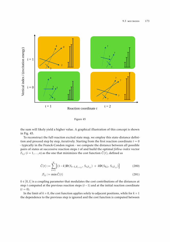
9.3 methods 173
0
23
4
i = 1
3 1
2
4
i = 0
Verti
cal i
ndex
i (e
xcita
tion
ener
gy)
Reaction coordinate t
??
?
?
?
??
?
t = 1 t = 2
Figure 45
the sum will likely yield a higher value. A graphical illustration of this concept is shownin Fig. 45.
To reconstruct the full-reaction excited state map, we employ this state-distance defini-tion and proceed step by step, iteratively. Starting from the first reaction coordinate t = 0- typically in the Franck-Condon region - we compute the distance between all possiblepairs of states at successive reaction steps t of and build the optimal follow-index vectorFt,i (i = 1, . . . ,n) as the one that minimizes the cost function C(t), defined as
C(t) :=n∑i=1
[(1− k)D(St−1,Ft−1,i , St,Ft,i ) + kD(S0,i , St,Ft,i )
](280)
Ft,i := min C(t) (281)
k ∈ [0,1] is a coupling parameter that modulates the cost contributions of the distances atstep t computed at the previous reaction steps (t − 1) and at the initial reaction coordinate(t = 0).
In the limit of k = 0, the cost function applies solely to adjacent positions, while for k = 1the dependence to the previous step is ignored and the cost function is computed between
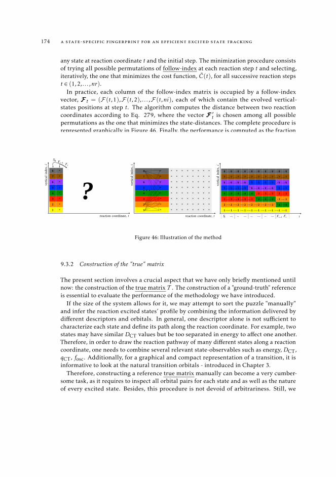
174 a state-specific fingerprint for an efficient excited state tracking
any state at reaction coordinate t and the initial step. The minimization procedure consistsof trying all possible permutations of follow-index at each reaction step t and selecting,iteratively, the one that minimizes the cost function, C(t), for all successive reaction stepst ∈ (1,2, . . . ,nr).
In practice, each column of the follow-index matrix is occupied by a follow-indexvector, FFF t = (F (t,1),F (t,2), . . . ,F (t,ni), each of which contain the evolved vertical-states positions at step t. The algorithm computes the distance between two reactioncoordinates according to Eq. 279, where the vector FFF ′t is chosen among all possiblepermutations as the one that minimizes the state-distances. The complete procedure isrepresented graphically in Figure 46. Finally, the performance is computed as the fractionof correctly-guessed follow-indexes with respect to the true matrix TTT , i.e., the full excitedstate map constructed by visual inspection of orbitals and descriptors.
8 * * * * * * * * *
7 * * * * * * * * *
6 * * * * * * * * *
5 * * * * * * * * *
4 * * * * * * * * *
3 * * * * * * * * *
2 * * * * * * * * *
1 * * * * * * * * *
Ft−1 Ft
S0
?vertic
alind
ex,i
reaction coordinate, t
8 * * * * * * * * *
7 * * * * * * * * *
6 * * * * * * * * *
5 * * * * * * * * *
4 * * * * * * * * *
3 * * * * * * * * *
2 * * * * * * * * *
1 * * * * * * * * *
. . .
vertic
alind
ex,i
reaction coordinate, t
8 8 8 8 8 8 8 8 8 8
7 7 7 7 7 7 7 7 7 7
6 6 6 6 5 5 5 5 6 6
5 5 5 5 6 6 6 6 5 5
4 4 4 4 4 3 3 3 3 3
3 3 3 3 3 4 4 4 2 2
2 2 2 2 2 2 2 2 4 4
1 1 1 1 1 1 1 1 1 1
S0 Ft−1 Ft⋯ ⋯ ⋯ ⋯ ⋯ ⋯ ⋯ver
tical
index,
it
Figure 46: Illustration of the method
9.3.2 Construction of the "true" matrix
The present section involves a crucial aspect that we have only briefly mentioned untilnow: the construction of the true matrix T . The construction of a "ground-truth" referenceis essential to evaluate the performance of the methodology we have introduced.
If the size of the system allows for it, we may attempt to sort the puzzle "manually"and infer the reaction excited states’ profile by combining the information delivered bydifferent descriptors and orbitals. In general, one descriptor alone is not sufficient tocharacterize each state and define its path along the reaction coordinate. For example, twostates may have similar DCT values but be too separated in energy to affect one another.Therefore, in order to draw the reaction pathway of many different states along a reactioncoordinate, one needs to combine several relevant state-observables such as energy, DCT,qCT, fosc. Additionally, for a graphical and compact representation of a transition, it isinformative to look at the natural transition orbitals - introduced in Chapter 3.
Therefore, constructing a reference true matrix manually can become a very cumber-some task, as it requires to inspect all orbital pairs for each state and as well as the natureof every excited state. Besides, this procedure is not devoid of arbitrariness. Still, we
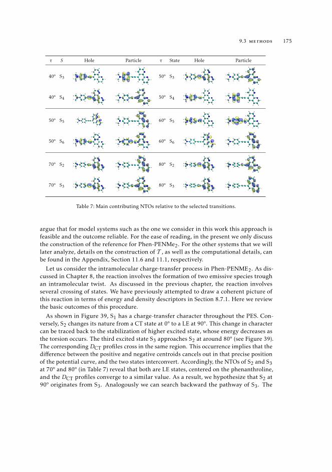
9.3 methods 175
τ S Hole Particle τ State Hole Particle
40° S3 50° S3
40° S4 50° S4
50° S5 60° S5
50° S6 60° S6
70° S2 80° S2
70° S3 80° S3
Table 7: Main contributing NTOs relative to the selected transitions.
argue that for model systems such as the one we consider in this work this approach isfeasible and the outcome reliable. For the ease of reading, in the present we only discussthe construction of the reference for Phen-PENMe2. For the other systems that we willlater analyze, details on the construction of T , as well as the computational details, canbe found in the Appendix, Section 11.6 and 11.1, respectively.
Let us consider the intramolecular charge-transfer process in Phen-PENME2. As dis-cussed in Chapter 8, the reaction involves the formation of two emissive species troughan intramolecular twist. As discussed in the previous chapter, the reaction involvesseveral crossing of states. We have previously attempted to draw a coherent picture ofthis reaction in terms of energy and density descriptors in Section 8.7.1. Here we reviewthe basic outcomes of this procedure.
As shown in Figure 39, S1 has a charge-transfer character throughout the PES. Con-versely, S2 changes its nature from a CT state at 0° to a LE at 90°. This change in charactercan be traced back to the stabilization of higher excited state, whose energy decreases asthe torsion occurs. The third excited state S3 approaches S2 at around 80° (see Figure 39).The corresponding DCT profiles cross in the same region. This occurrence implies that thedifference between the positive and negative centroids cancels out in that precise positionof the potential curve, and the two states interconvert. Accordingly, the NTOs of S2 and S3at 70° and 80° (in Table 7) reveal that both are LE states, centered on the phenanthroline,and the DCT profiles converge to a similar value. As a result, we hypothesize that S2 at90° originates from S3. Analogously we can search backward the pathway of S3. The
176 a state-specific fingerprint for an efficient excited state tracking
energy profile (in Figure 39) suggests that between 40° and 50° S3 lies very close to S4.Besides, the NTOs (in Table 7) indicate that S3 is a ππ∗ state at 40° centered on theN-dimethylaminophenyl group. The same ππ∗ state shifts to S4 at 50°; vice-versa, S4 at50° matches the character of S3 at 60°. The fosc curves (in Figure 39) cross in the sameregion. These pieces of evidence suggest that the S3 and S4 states intersect in the 40°-50°region. Altogether we may conclude that the LE state (S2) at 90° originates from S4. Inaddition, the S5 ad S6 curves in 39 hint to the presence of a crossing region between 50°and 60°. Analogously, the corresponding NTOs in Figure 7 point in the same direction.The considerations above allow us to construct a preliminary picture of the evolution ofthe first six excited states along the reaction coordinate. This brief description, althoughqualitative, is in agreement the analysis in Chapter 8 [7].
As previously alluded to, both the energy and the descriptors that we use to inspectthe nature of the excited states are computed at a predefined level of theory (method andbasis-set) at which the calculations are performed. Therefore, the resulting descriptionmay sensibly vary according to the applied methodology. The inclusion or not of solventeffects may also affect the outcome. As a consequence, the "fingerprint" strategy discussedhere is as accurate as the method used to calculate the potential energy surfaces. Ingeneral, though, it is always advisable to choose a reliable method (as a start), such thatthe excited state densities are reliable.
Besides, one should be sure to take into account a sufficient number of excited states,and that the same states, in terms of character, can be found at each step of the reactioncoordinate. Although it is not always possible to guesstimate the relative positioning ofthe vertical states, visually inspecting the lowest orbitals, for relatively small systems asthe one discussed here, this procedure is generally accessible and simplifies this process.
Using the same strategy, we have constructed analogous excited state reference mapsfor the photo-induced proton-transfer reaction in CPDNO and for the charge transfer inDMABN. All the related data are collected in Section 11.6, in Appendix.
9.4 results
We have tested our tracking protocol on three different systems, namely CPDNO, Phen-PENMe2 and DMABN. We refer to the discussion in Chapter 8 for the definition of thereaction coordinate, and description of the photoinduced reaction of each system. Just asdiscussed previously, we have sliced each reaction coordinate in a number of step - eightfor CPDNO and ten for the other systems and calculated a number of vertical states at allthe different steps of the reaction. In the present, we analyze the first five vertical statesfor CPDNO and the first 6 for Phen-PENMe2 and DMABN.
We now examine the performance curves trends calculated on each different systemusing increasing values of k ranging from 0 to 1. We recall that k modulates the costcontributions of the distances at step t computed at the previous reaction steps (t − 1) andat the initial reaction coordinate (t = 0). Similar patterns can be observed in all system. Inall cases, low values of k yield larger differences with respect to the ground truth referencestate map in Table 8. Close to the Franck-Condon region the character of all states is close
9.5 overlap-based methods 177
to the one that each state has at the initial point of the reaction. Further on in the reaction,the nature of each vertical state evolves and can end changing significantly from the firstassignment. Therefore, larger values of k reproduce more accurately the reference map,as the state-distance D is calculated with respect to the state vector at the previous stepin the reaction, rather than with the initial step. Differently stated, as the excited statespathways gradually change along the reaction coordinate, it is more effective to comparevertical states at adjacent positions rather than including the contribution of the initialstate-vector.
In Phen-PENMe2 the performance values oscillates between two positions, with amaximum value of 0.89. The fingerprint method reveals correctly all the crossing of states.The only difference appears at step seven in the reaction coordinate, corresponding toτ = 60°, were the state-fingerprint method individuates a crossing between states five andsix, which is not present in the reference map. The paired distance values of the fifth andsixth vertical states at τ = 60° and τ = 70° is very little, ≈ 0.2 Å, which makes it difficultto unambiguously determine the relative position of these two states. The overall pictureproduced by the two methods remains very similar.
An analogous analysis can be done for the DMABN, with some additional complexity.For DMABN the construction of the reference matrix is not as straightforward as it isin the previous case, as the map is not fully consistent. At step seven of the reactioncoordinate (τ = 60°) a new vertical excited state appears, which cannot be "matched"with any of the states at the previous steps. The orbital shape of this state cannot beimmediately recognized in the state-vectors at previous steps of the reaction. Besides, atsuccessive steps of the reaction this same state descends to the fifth position. To restorethe consistency one could simply add few more vertical state, however all vertical statesare more and more mixed, making it difficult to assign the character unambiguously.We are left with some "intruder" states that will be certainly not correctly reproducedusing our procedure. However, as these states appear quite high in energy, and theydo not connect with the lower energy states, we can assume that their relevance in thephotochemical process is negligible. Hence, we do not account for these "intruder" statesin the performance measure. As shown in Table 8 (right panels), all state crossings thathappen before the intruder state comes in are correctly retrieved by the method, thereforereaching an almost-optimal performance.
The third system we consider is CPDNO, shown in Table 8 (central panels). By visualinspecting the orbitals and descriptors we recognized only one state crossing, happeningbetween states 1 and 2 at t = 2. Our method retrieves this transition correctly, leaving allother positions unchanged. Consequently, the computed performance is 1.0.
9.5 overlap-based methods
One possible alternative to track the state evolution along a reaction coordinate is todefine the state-distance as the overlap between the wave-functions of all pair of states at
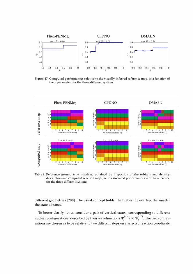
178 a state-specific fingerprint for an efficient excited state tracking
Phen-PENMe2 CPDNO DMABN
Figure 47: Computed performances relative to the visually-inferred reference map, as a function ofthe k parameter, for the three different systems.
Phen-PENMe2 CPDNO DMABN
refe
renc
em
ap
1 2 3 4 5 6 7 8 9 10reaction coordinate (t)
123456
verti
cal s
tate
(i)
1 2 3 4 5 6 7 8reaction coordinate (t)
1
2
3
4
5
verti
cal s
tate
(i)
1 2 3 4 5 6 7 8 9 10reaction coordinate (t)
123456
verti
cal s
tate
(i)
com
pu
ted
map
1 2 3 4 5 6 7 8 9 10reaction coordinate (t)
123456
verti
cal s
tate
(i)
P = 0.89, k = 0.90
1 2 3 4 5 6 7 8reaction coordinate (t)
1
2
3
4
5
verti
cal s
tate
(i)
P = 1.00, k = 0.90
1 2 3 4 5 6 7 8 9 10reaction coordinate (t)
123456
verti
cal s
tate
(i)
P = 0.84, k = 0.90
Table 8: Reference ground true matrices, obtained by inspection of the orbitals and density-descriptors and computed reaction maps, with associated performances w.r.t. to reference,for the three different systems
different geometries [280]. The usual concept holds: the higher the overlap, the smallerthe state distance.
To better clarify, let us consider a pair of vertical states, corresponding to different
nuclear configurations, described by their wavefunctions Ψ(t)i and Ψ
(t′)j . The two configu-
rations are chosen as to be relative to two different steps on a selected reaction coordinate.
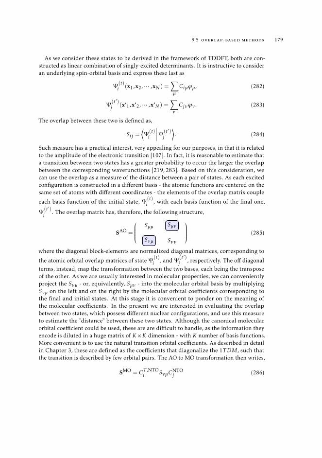
9.5 overlap-based methods 179
As we consider these states to be derived in the framework of TDDFT, both are con-structed as linear combination of singly-excited determinants. It is instructive to consideran underlying spin-orbital basis and express these last as
Ψ(t)i (x1,x2, · · · ,xN ) =
∑µ
Ciµϕµ, (282)
Ψ(t′)j (x’1,x’2, · · · ,x’N ) =
∑ν
Cjνϕν . (283)
The overlap between these two is defined as,
Sij =⟨Ψ
(t)i
∣∣∣∣∣ Ψ (t′)j
⟩. (284)
Such measure has a practical interest, very appealing for our purposes, in that it is relatedto the amplitude of the electronic transition [107]. In fact, it is reasonable to estimate thata transition between two states has a greater probability to occur the larger the overlapbetween the corresponding wavefunctions [219, 283]. Based on this consideration, wecan use the overlap as a measure of the distance between a pair of states. As each excitedconfiguration is constructed in a different basis - the atomic functions are centered on thesame set of atoms with different coordinates - the elements of the overlap matrix couple
each basis function of the initial state, Ψ(t)i , with each basis function of the final one,
Ψ(t′)j . The overlap matrix has, therefore, the following structure,
SAO =
Sµµ Sµν
Sνµ Sνν
(285)
where the diagonal block-elements are normalized diagonal matrices, corresponding to
the atomic orbital overlap matrices of state Ψ(t)i , and Ψ
(t′)j , respectively. The off diagonal
terms, instead, map the transformation between the two bases, each being the transposeof the other. As we are usually interested in molecular properties, we can convenientlyproject the Sνµ - or, equivalently, Sµν - into the molecular orbital basis by multiplyingSνµ on the left and on the right by the molecular orbital coefficients corresponding tothe final and initial states. At this stage it is convenient to ponder on the meaning ofthe molecular coefficients. In the present we are interested in evaluating the overlapbetween two states, which possess different nuclear configurations, and use this measureto estimate the "distance" between these two states. Although the canonical molecularorbital coefficient could be used, these are are difficult to handle, as the information theyencode is diluted in a huge matrix of K ×K dimension - with K number of basis functions.More convenient is to use the natural transition orbital coefficients. As described in detailin Chapter 3, these are defined as the coefficients that diagonalize the 1TDM, such thatthe transition is described by few orbital pairs. The AO to MO transformation then writes,
SMO = CT ,NTOi SνµC
NTOj (286)
180 a state-specific fingerprint for an efficient excited state tracking
Since the CNTOi and CNTO
j coefficients are not calculated in the same basis, it is convenient
to normalize each column of the SMO matrix. We denote the normalized molecular orbitalmatrix as SMO. As we adopt the NTO formalism, SMO has a compact form: the elementsthat actually describe the excitation are very little in number and can be easily isolatedto obtain a clear and direct interpretation of the process. In particular, the relevantelements are those corresponding to the overlap between the atomic orbitals matrixcolumns associated with the highest NTO eigenvalues. By definition, these last are thosecorresponding to the HOMO and LUMO orbitals and, occasionally, to a few adjacentorbital pairs. In turn, the nonzero elements of the SMO matrix that we are interested tolook at constitute a sub-square-matrix of reduced size. For example, if the nonzero NTOeigenvalues are only four, the sub-matrix will have dimensions of 2 × 2. Among these,the diagonal elements of the SNTO matrix are those that couple each relevant molecularorbital at one geometry with the same orbitals at a different geometry. A convenient way totranslate this reduced-overlap-matrix into a quantitative measure of the overlap betweenthe associated density distributions is to calculate its trace. Given N as the number ofrow (and columns) of SNTO, we define the distance between any two states as the inverseof the trace of the normalized overlap matrix computed between the state St,i and St,j ,divided by N .
d = (T r(SNTO)/N )−1. (287)
By consequence, the distance between a pair of states will be large whenever the trace ofthe normalized overlap matrix is small, and small otherwise.
9.5.1 Performance of the overlap method
We have applied the overlap formalism to the same three systems described in the previoussection, by plugging the state distance as defined in Eq. 279 in the cost function of Eq. 281to find the follow index map F that minimizes it. The resulting state map is then comparedto both the reference map computed by visual inspection and to the one found by the"fingerprint" protocol described in the previous section. For both these comparison wecompute the performance (i.e., the similarity between matrices) as a function of k ∈ [0,1].As shown in Figure 48, in the case of CPDNO and DMABN the three methods yieldcomparable results, as the values of similarity between maps (denoted as performanceP ) ranges between P ∼ 0.8 and P ∼ 0.94 for k > 0.5. In the case of Phen-PENME2, on thecontrary, performance values are very low (around P ∼ 0.3/0.4 for all values of k). Thisapparently high discrepancy, however, can be explained by visualizing the detailed mapsgiven by the three protocols at a fixed value of k. The comparison, shown in Table 9, showsthat the low performance is mostly due to a propagation of an initial error occurring atthe first reaction steps (t = 1,2). In fact, important state crossing between low-energystates are indeed recognized by all methods (e.g. states 3,4 at t = 5,6 and states 2,3 att = 8,9), even though the overlap method crosses the wrong indexes due to a series offalse crossings happening at t = 1,2.
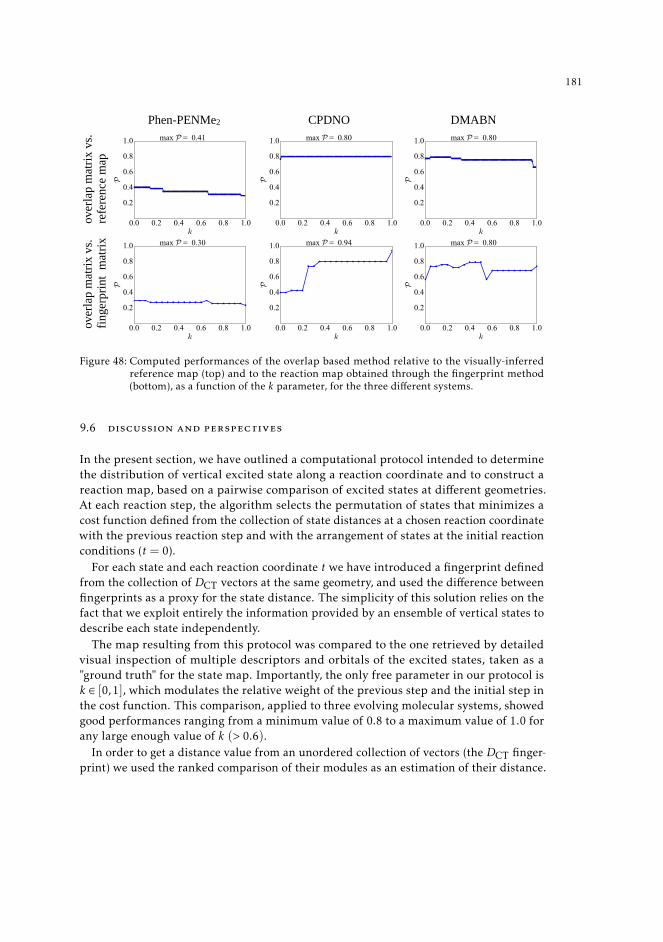
9.6 discussion and perspectives 181
Phen-PENMe2 CPDNO DMABN
over
lap
mat
rix v
s. re
fere
nce
map
over
lap
mat
rix v
s. fin
gerp
rint
mat
rix
Figure 48: Computed performances of the overlap based method relative to the visually-inferredreference map (top) and to the reaction map obtained through the fingerprint method(bottom), as a function of the k parameter, for the three different systems.
9.6 discussion and perspectives
In the present section, we have outlined a computational protocol intended to determinethe distribution of vertical excited state along a reaction coordinate and to construct areaction map, based on a pairwise comparison of excited states at different geometries.At each reaction step, the algorithm selects the permutation of states that minimizes acost function defined from the collection of state distances at a chosen reaction coordinatewith the previous reaction step and with the arrangement of states at the initial reactionconditions (t = 0).
For each state and each reaction coordinate t we have introduced a fingerprint definedfrom the collection of DCT vectors at the same geometry, and used the difference betweenfingerprints as a proxy for the state distance. The simplicity of this solution relies on thefact that we exploit entirely the information provided by an ensemble of vertical states todescribe each state independently.
The map resulting from this protocol was compared to the one retrieved by detailedvisual inspection of multiple descriptors and orbitals of the excited states, taken as a"ground truth" for the state map. Importantly, the only free parameter in our protocol isk ∈ [0,1], which modulates the relative weight of the previous step and the initial step inthe cost function. This comparison, applied to three evolving molecular systems, showedgood performances ranging from a minimum value of 0.8 to a maximum value of 1.0 forany large enough value of k (> 0.6).
In order to get a distance value from an unordered collection of vectors (the DCT finger-print) we used the ranked comparison of their modules as an estimation of their distance.
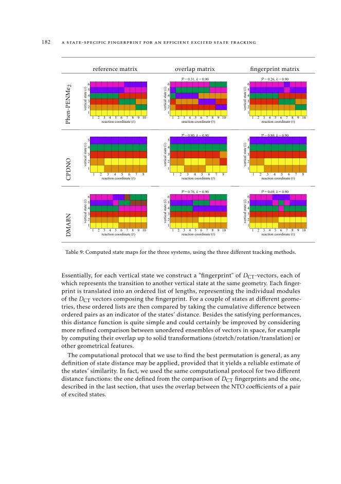
182 a state-specific fingerprint for an efficient excited state tracking
reference matrix overlap matrix fingerprint matrixP
hen-
PE
NM
e 2
1 2 3 4 5 6 7 8 9 10reaction coordinate (t)
123456
verti
cal s
tate
(i)
1 2 3 4 5 6 7 8 9 10reaction coordinate (t)
123456
verti
cal s
tate
(i)
P = 0.31, k = 0.90
1 2 3 4 5 6 7 8 9 10reaction coordinate (t)
123456
verti
cal s
tate
(i)
P = 0.26, k = 0.90
CP
DN
O
1 2 3 4 5 6 7 8reaction coordinate (t)
1
2
3
4
5
verti
cal s
tate
(i)
1 2 3 4 5 6 7 8reaction coordinate (t)
1
2
3
4
5
verti
cal s
tate
(i)
P = 0.80, k = 0.90
1 2 3 4 5 6 7 8reaction coordinate (t)
1
2
3
4
5
verti
cal s
tate
(i)
P = 0.80, k = 0.90
DM
AB
N
1 2 3 4 5 6 7 8 9 10reaction coordinate (t)
123456
verti
cal s
tate
(i)
1 2 3 4 5 6 7 8 9 10reaction coordinate (t)
123456
verti
cal s
tate
(i)
P = 0.76, k = 0.90
1 2 3 4 5 6 7 8 9 10reaction coordinate (t)
123456
verti
cal s
tate
(i)
P = 0.69, k = 0.90
Table 9: Computed state maps for the three systems, using the three different tracking methods.
Essentially, for each vertical state we construct a "fingerprint" of DCT-vectors, each ofwhich represents the transition to another vertical state at the same geometry. Each finger-print is translated into an ordered list of lengths, representing the individual modulesof the DCT vectors composing the fingerprint. For a couple of states at different geome-tries, these ordered lists are then compared by taking the cumulative difference betweenordered pairs as an indicator of the states’ distance. Besides the satisfying performances,this distance function is quite simple and could certainly be improved by consideringmore refined comparison between unordered ensembles of vectors in space, for exampleby computing their overlap up to solid transformations (stretch/rotation/translation) orother geometrical features.
The computational protocol that we use to find the best permutation is general, as anydefinition of state distance may be applied, provided that it yields a reliable estimate ofthe states’ similarity. In fact, we used the same computational protocol for two differentdistance functions: the one defined from the comparison of DCT fingerprints and the one,described in the last section, that uses the overlap between the NTO coefficients of a pairof excited states.

9.6 discussion and perspectives 183
In conclusion, the overall advantage of the method proposed in this chapter lies in itssimplicity. This methodology provides a simple and straightforward solution to trackexcited states along a reaction path, without the need for any parameter optimization,neither requiring the knowledge of the energy profiles.

10CONCLUS ION AND PERSPECT IVES
10.1 outline
The objective of this thesis was to devise, construct, and apply a cost-effective approachto calculate photophysical properties of molecular systems, based on ad-hoc densitydescriptors, to characterize the relevant photophysical pathways for the many processestaking place at the excited state. The result of our investigation is a collection of TDDFT-based protocols, which can be applied to characterize the excited-state potential energysurfaces of molecular systems, based on the knowledge of ground and excited statedensities.
The inherent complexity in the modeling of excited-state processes is related to thefact that the molecular systems under study are typically out of equilibrium, perturbedupon the interaction with light. The computational setup that we have devised meetsthis context in that it allows us to monitor the evolution of excited states along a reactioncoordinate.
The key observable and leitmotif of our investigations is the electronic density, whichholds the response of the system to the light-induced perturbation. We have interpretedsuch observable through purposely defined descriptors, which we have used to track thechanges in the electronic density distributions along photochemical pathways.
Besides defining an adapted metric for the excited state processes under analysis,the density descriptors that we have proposed and employed yield novel insights onrelevant physical properties of the molecular systems, translating computational outcomesin simple chemical and physical concepts (such for instance the strength and spatialamplitude of the charge separation produced by an electronic excitation).
In Chapter 4, we have systematically analyzed the nature and impact of the densityrelaxation involved in the post-linear response treatment of time-dependent densityfunctional theory on the measure of charge separation length that characterizes thehole/particle generation, i.e., the DCT index. For this purpose, we have considered afamily of push-pull dyes of increasing length, where the primary hole/particle charge-separation distance grows with the length of the molecular skeleton. Assessing theinfluence of the use of different density functional approximations on the topology of thedensity distribution generated upon transition allowed us to conclude that such responsestrongly depends on the kernel used for generating the exciton. Moreover, we showedthat, qualitatively, both unrelaxed and relaxed densities deliver a consistent assessmentof the nature of the excited states. From a quantitative standpoint, though, we observedsignificant discrepancies in the charge transfer distance for electronic transitions havingsubstantial charge transfer (CT) character, independently of the nature of the exchange-correlation functional used.
185
186 conclusion and perspectives
Next, in Chapter 5 we tested the ability of the DCT to reckon the nature of excitedstates along a full reaction. Using a prototype excited-state proton transfer reaction asa test case, we showed that density-based descriptors (such as the DCT index) could besafely used to analyze excited states qualitatively and quantitatively. More precisely,the DCT provided a good description of the electronic rearrangements occurring in thephotochemical reaction studied, both using density functional and multiconfigurationalmethods - here CASSCF-CASPT. Our results suggest that the DCT could be employed, justas the energy, to locate minima, on potential energy surfaces.
Our modeling of the excited-state energy profiles was complemented, in Chapter 6,with a diagnostic analysis to probe the accuracy of TDDFT methods. In this context,we proposed a new index, MAC, for the detection of erratic TDDFT behavior, pointingout the region of excited-state potential energy curves claiming for a more in-depthdescription. The MAC diagnostic analysis allows us to identify ghost- and spurious-low-lying excitations, that may result from a particular choice of approximated densityfunctional. In Chapter 7 we used such index to characterize singlet and triplet excitationsin metal-containing complexes. Overall, in Chapter 6 and 7 we have rationalized whatthe pitfalls of TDDFT are, what is the reason for their appearance and under whatcircumstances existing approximations work well or fail. By complementing the MACdiagnostic analysis with experimental measurements, we were able to judge the reliabilityof a chosen methodology.
In Chapter 8, we extended our computational setup to characterize excited-state path-ways in the case of reactions involving a profound structural change. This investigationfits in the broader context of the computer-assisted design of new molecular architectureswith peculiar photochemical traits able, for instance, to store energy through reversibleconformational changes induced by electronic excitations. In particular, we extendedthe definition of a previously-defined index,Π [2], to the case of the internal conversionbetween excited states, and applied it to investigate potential energy surfaces of low-lyingexcited states far Franck-Condon region, that is, in regions involved, for instance, in theradiative and non-radiative decay patterns.
Finally, in Chapter 9 we have introduced a new methodology to track the electronicstates of interest along the nuclear trajectory, based on the definition of a state-specificfingerprint that leverages the full information contained in the transition vectors tocharacterize any excited state uniquely.
With the development of the state-tracking algorithm and the implementation ofseveral density-descriptors outlined in this thesis, we have proposed a cost-effectiveway of addressing the challenge of disclosing excited state pathways in the modelingof photophysical processes. Indeed, we have shown how this is often crucial for theunderstanding and prediction of such phenomena. As for the results discussed in Chapter9, further study into the behavior of the fingerprint-method is desirable - for instance byusing different molecular architectures, by including metal complexes, or by consideringa larger number of states. Nevertheless, the performance and versatility of this modellooks, thus far, rather promising and should prompt further development in the directionof new-efficient excited-states optimization algorithms.
10.2 methodology and future research 187
10.2 methodology and future research
The application of TDDFT based modeling and density descriptors to the complex phe-nomenology of photochemical processes raises several methodological questions, whichrange from the large simplifications made in the theoretical models we apply to theconstraints and lack of kinetic considerations in our approach. The possible strategiesof the theoretical chemist’ to investigate photochemical and photophysical issues aremanifold, and it would be an utter simplification to attempt here a comprehensive outlineof a discussion of such vast scope. At the same time, we believe that there are a few pointsthat deserve mention, undoubtedly less general, and specifically related to the results thatwe have discussed in this work.
In the last two chapters, in particular, we have employed different metrics to recognizeexcited states of different nature along specific reaction coordinates to infer the excitedstate pathway of each state, first with the Π index, and secondly with the so-called finger-print method. One of the most arguable features of these approaches is that the actualinterpretation of the photophysical pathway depends on the accuracy of underlying densi-ties, and thus on the quantum mechanical method used to generate these latter. Secondly,the overall picture that we obtain is qualitative, in the sense that what we obtain is apossible survey of accessible decay channels, rather than a precise characterization offunnel regions. However, in this somewhat simplistic view lies also the beauty of ourapproach, which is intended to provide a computationally inexpensive characterizationof the excited state potential landscapes. As such, the indexes discussed herein are notintended to substitute the classical route of excited state exploration but more to provideeasy-to-compute and easy-to-interpret descriptions of excited-state phenomena, whichcan be computed – on the fly- to allow both the identification of critical area for TDDFTapproaches and the qualitative identification of possible reactions paths.
In a very general sense, the density descriptors that we have proposed and appliedthroughout this work condense the information contained in objects such as the differencedensity matrix in more compact and easy-to-interpret metrics, which provide an attractivealternative to more complex wavefunction analysis approaches. As such, they can aid inthe rational design of molecular architectures for specific applications by, for example,serving as an optimization target. In fact, part of our current ongoing research focuses onthe application of these tools to devise novel Ru(II) photosensitizers with exceptional char-acteristics for anti-cancer activity (intense absorption in the phototherapeutic window andstable, long-lived low-lying triplet states).
To conclude, the new "fingerprint" metric that we have proposed in Chapter 9 wasproven to efficiently track the electronic states of interest along the nuclear trajectory.These preliminary results suggest that it might even be possible to employ the state-specific fingerprints in automatized diabatization schemes, by transforming the statessuch that the DCT vectors change as little as possible. Further applications are alsopossible in theoretical chemistry method development, where DCT fingerprints, that arebased on results from less costly TDDFT computations, could be used to aid the design ofsensible active spaces for multiconfigurational calculations.


Part IV
APPENDIX

11SUPPLEMENTARY MATER IALS
11.1 computational details
Throughout this work we have chosen different organic chromophores, such as Phen-PENMe2, DMABN, CPDNO as test cases to exemplify the insights that density-basedindexes may bring to the description excited state processes. All calculations - wherenot differently specified - were performed with a development version of the Gaussianprogram [145]. In general, the evaluation of all density-based indexes DCT, MAC andΠ was done using self made freely distributed programs available at www.quanthic.fr,although the DCT index can also be directly computed using the commercial release ofthe Gaussian software [145]. In general, for all systems we have have applied the samecomputational protocols, consisting of the following steps:
• preliminary geometry optimization using ground state DFT [32], to fully relax thestructure. In "scan" calculation all degrees of freedom are relaxed except for thatalong which the reaction occurs;
• frequency calculation to characterize each structure as minimum or transition state;
• TDDFT calculation to obtain the excited state levels at each geometry (and calcula-tion of density based indices, such as DCT, MAC, Π).
The details of the calculations reported in each chapter are summarized in Table 10.Natural transition orbitals [92] (NTO) relative to the ten lowest electronic transitions werealso computed for a visual interpretation of the nature electronic transitions. All orbitalsare collected in section 11.5.
191
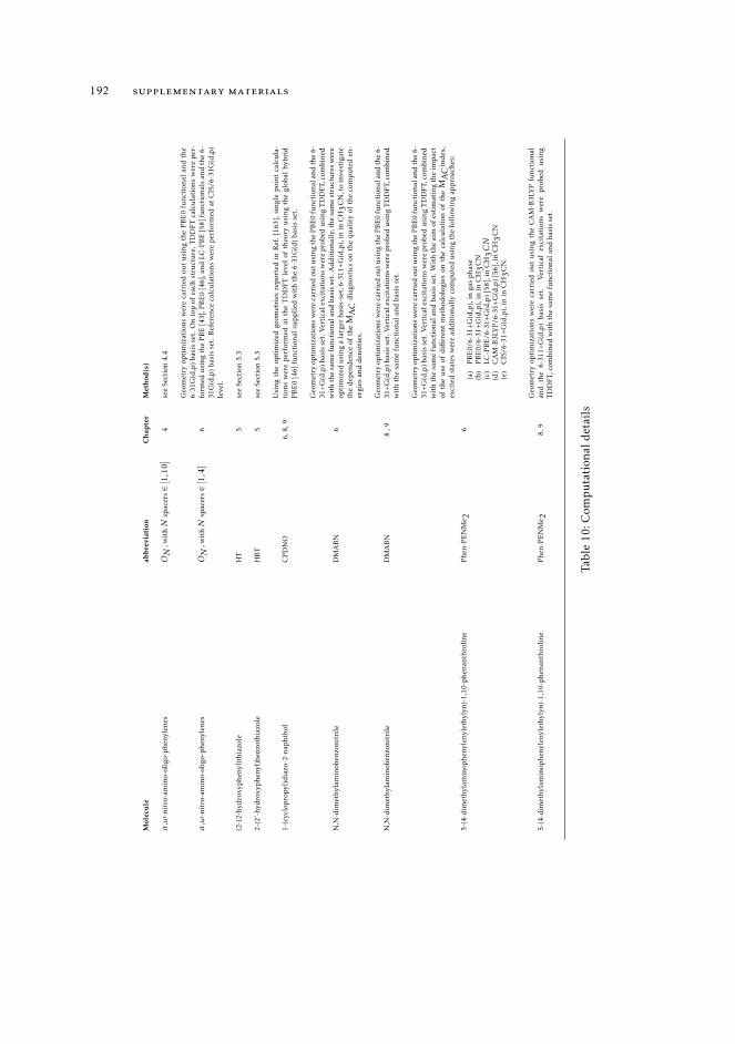
192 supplementary materials
Mol
ecu
leab
bre
viat
ion
Ch
apte
rM
eth
od(s
)
α,ω
-nit
ro-a
min
o-ol
igo-
phe
nyle
nes
ON
,wit
hN
spac
ers∈[
1,10
]4
see
Sect
ion
4.4
α,ω
-nit
ro-a
min
o-ol
igo-
phe
nyle
nes
ON
,wit
hN
spac
ers∈[
1,4]
6
Geo
met
ryop
tim
izat
ions
wer
eca
rrie
dou
tu
sing
the
PB
E0
func
tion
alan
dth
e6-
31G
(d,p
)ba
sis
set.
On
top
ofea
chst
ruct
ure
,TD
DFT
calc
ula
tion
sw
ere
per
-fo
rmed
usi
ngth
eP
BE
[43]
,PB
E0
[46]
,and
LC-P
BE
[58]
func
tion
als
and
the
6-31
G(d
,p)
basi
sse
t.R
efer
ence
calc
ula
tion
sw
ere
per
form
edat
CIS
/6-3
1G(d
,p)
leve
l.
(2-(
2-hy
dro
xyp
heny
l)th
iazo
leH
T5
see
Sect
ion
5.3
2-(2
’-hy
dro
xyp
heny
l)be
nzot
hiaz
ole
HB
T5
see
Sect
ion
5.3
1-(c
yclo
pro
pyl)
dia
zo-2
-nap
htho
lC
PD
NO
6,8,
9U
sing
the
opti
miz
edge
omet
ries
rep
orte
din
Ref
.[1
63],
sing
lep
oint
calc
ula
-ti
ons
wer
ep
erfo
rmed
atth
eT
DD
FTle
vel
ofth
eory
usi
ngth
egl
obal
hybr
idP
BE
0[4
6]fu
ncti
onal
sup
pli
edw
ith
the
6-31
G(d
)bas
isse
t.
N,N
-dim
ethy
lam
inob
enzo
nitr
ile
DM
AB
N6
Geo
met
ryop
tim
izat
ions
wer
eca
rrie
dou
tusi
ngth
eP
BE
0fu
ncti
onal
and
the
6-31
+G
(d,p
)bas
isse
t.V
erti
cale
xcit
atio
nsw
ere
pro
bed
usi
ngT
DD
FT,c
ombi
ned
wit
hth
esa
me
func
tion
alan
dba
sis
set.
Ad
dit
iona
lly,
the
sam
est
ruct
ure
sw
ere
opti
miz
edu
sing
ala
rger
basi
s-se
t,6-
311+
G(d
,p),
inin
CH
3C
N,t
oin
vest
igat
eth
ed
epen
den
ceof
the
MA
Cd
iagn
osti
cson
the
qual
ity
ofth
eco
mp
ute
den
-er
gies
and
den
siti
es.
N,N
-dim
ethy
lam
inob
enzo
nitr
ile
DM
AB
N8
,9G
eom
etry
opti
miz
atio
nsw
ere
carr
ied
outu
sing
the
PB
E0
func
tion
alan
dth
e6-
31+
G(d
,p)b
asis
set.
Ver
tica
lexc
itat
ions
wer
ep
robe
du
sing
TD
DFT
,com
bine
dw
ith
the
sam
efu
ncti
onal
and
basi
sse
t.
5-(4
-dim
ethy
lam
inop
heny
leny
leth
ylyn
)-1,
10-p
hena
nthr
olin
eP
hen-
PE
NM
e 26
Geo
met
ryop
tim
izat
ions
wer
eca
rrie
dou
tusi
ngth
eP
BE
0fu
ncti
onal
and
the
6-31
+G
(d,p
)bas
isse
t.V
erti
cale
xcit
atio
nsw
ere
pro
bed
usi
ngT
DD
FT,c
ombi
ned
wit
hth
esa
me
func
tion
alan
dba
sis
set.
Wit
hth
eai
mof
esti
mat
ing
the
imp
act
ofth
eu
seof
diff
eren
tm
etho
dol
ogie
son
the
calc
ula
tion
ofth
eM
AC
ind
ex,
exci
ted
stat
esw
ere
add
itio
nall
yco
mp
ute
du
sing
the
foll
owin
gap
pro
ache
s:
(a)
PB
E0/
6-31
+G
(d,p
),in
gas
pha
se(b
)P
BE
0/6-
31+
G(d
,p),
inin
CH
3C
N(c
)LC
-PB
E/6
-31+
G(d
,p)[
58],
inC
H3CN
(d)
CA
M-B
3LY
P/6
-31+
G(d
,p)[
56],
inC
H3
CN
(e)
CIS
/6-3
1+G
(d,p
),in
inC
H3
CN
.
5-(4
-dim
ethy
lam
inop
heny
leny
leth
ylyn
)-1,
10-p
hena
nthr
olin
eP
hen-
PE
NM
e 28,
9G
eom
etry
opti
miz
atio
nsw
ere
carr
ied
out
usi
ngth
eC
AM
-B3L
YP
func
tion
alan
dth
e6-
311+
G(d
,p)
basi
sse
t.V
erti
cal
exci
tati
ons
wer
ep
robe
du
sing
TD
DFT
,com
bine
dw
ith
the
sam
efu
ncti
onal
and
basi
sse
t.
Tabl
e10
:Com
pu
tati
onal
det
ails
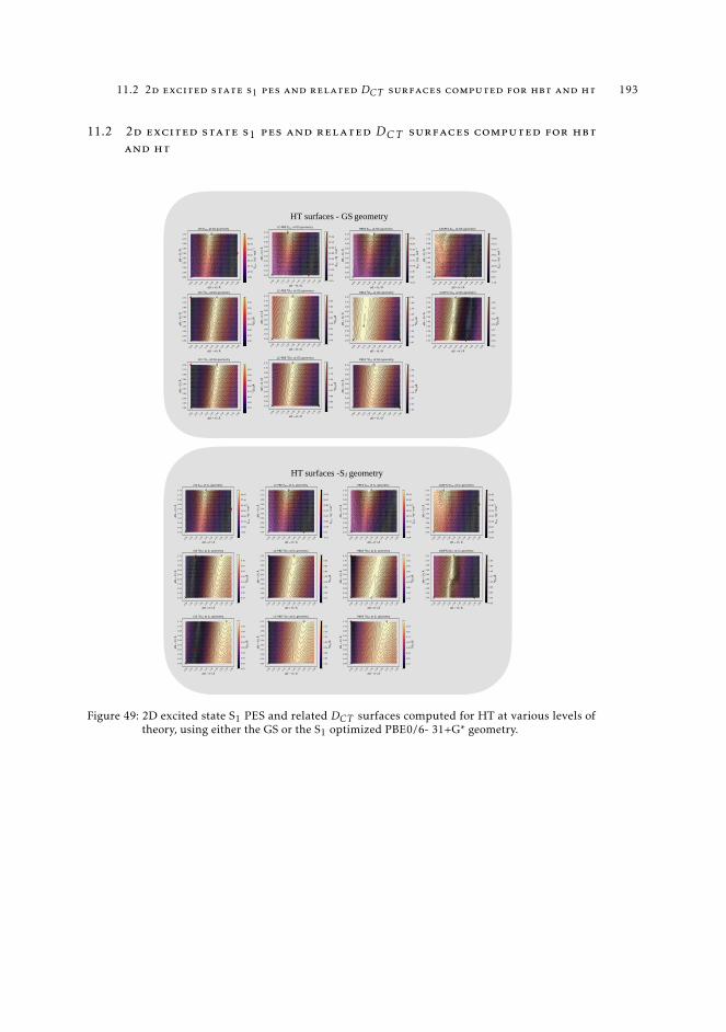
11.2 2d excited state s1 pes and related DCT surfaces computed for hbt and ht 193
11.2 2d excited state s1 pes and related DCT surfaces computed for hbt
and ht
HT surfaces -S1 geometry
HT surfaces - GS geometry
Figure 49: 2D excited state S1 PES and related DCT surfaces computed for HT at various levels oftheory, using either the GS or the S1 optimized PBE0/6- 31+G* geometry.
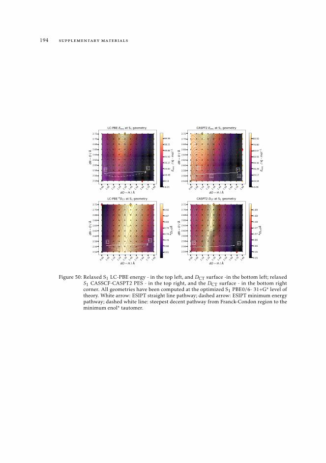
194 supplementary materials
E* K* K*
Testo
E*
a)
b) c) d)
E* K*K*E*
Figure 50: Relaxed S1 LC-PBE energy - in the top left, and DCT surface -in the bottom left; relaxedS1 CASSCF-CASPT2 PES - in the top right, and the DCT surface - in the bottom rightcorner. All geometries have been computed at the optimized S1 PBE0/6- 31+G* level oftheory. White arrow: ESIPT straight line pathway; dashed arrow: ESIPT minimum energypathway; dashed white line: steepest decent pathway from Franck-Condon region to theminimum enol* tautomer.
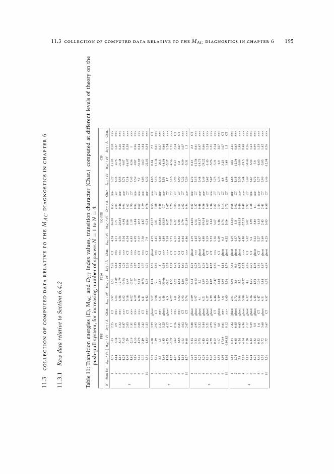
11.3 collection of computed data relative to the MAC diagnostics in chapter 6 19511.3
collectionofcomputeddatarelativetotheMAC
diagnosticsinchapter6
11.3.1
Raw
data
rela
tive
toSe
ctio
n6.
4.2
Tabl
e11
:Tra
nsi
tion
ener
gies
(E),
MA
Can
dD
CT
ind
exva
lues
,tr
ansi
tion
char
acte
r(C
har
.)co
mp
ute
dat
diff
eren
tle
vels
ofth
eory
onth
ep
ush
-pu
llsy
stem
,for
incr
easi
ngnu
mbe
rof
spac
ersN
=1
toN
=4.
PB
EP
BE
0LC
-PB
EC
IS
NSt
ate
Nr.
Eex
c/
eVM
AC
/eV
DC
T/
ÅC
har.
Eex
c/
eVM
AC
/eV
DC
T/
ÅC
har.
Eex
c/
eVM
AC
/eV
DC
T/
ÅC
har.
Eex
c/
eVM
AC
/eV
DC
T/
ÅC
har.
1
13.
391.
032.
25C
T3.
971.
582.
25C
T4.
24-1
6.88
0.53
ππ∗
5.22
-15.
030.
58ππ∗
23.
64-7
.44
0.9
ππ∗
4.04
-11.
890.
68ππ∗
4.71
1.71
2.04
CT
5.33
-2.7
51.
47ππ∗
34.
16-3
.17
1.32
ππ∗
4.58
-12.
790.
64ππ∗
4.76
-20.
650.
46ππ∗
5.55
-21.
480.
46ππ∗
44.
23-7
.43
0.87
ππ∗
4.62
-3.6
41.
26ππ∗
5.04
-6.9
40.
94ππ∗
5.71
-9.0
70.
94ππ∗
54.
431.
292.
05C
T5.
181.
472.
05C
T6.
340.
841.
62C
T7.
14-1
6.97
0.58
ππ∗
64.
62-2
.18
1.51
ππ∗
6.02
-2.8
71.
76ππ∗
6.83
1.19
1.95
CT
7.43
-8.5
61
ππ∗
75.
19-1
.36
1.55
ππ∗
6.19
-1.0
71.
87ππ∗
6.95
-6.8
40.
84ππ∗
7.59
-9.8
70.
96ππ∗
85.
29-1
.78
2.08
ππ∗
6.28
3.71
2.33
CT
7.17
-12.
30.
67ππ∗
7.7
-51.
890.
24ππ∗
95.
352.
492.
42C
T6.
41-0
.75
1.57
ππ∗
7.38
-4.8
71.
29ππ∗
8.03
-0.6
21.
84ππ∗
105.
59-1
.89
1.53
ππ∗
6.42
1.38
1.71
CT
7.9
-6.3
10.
76ππ∗
8.32
-22.
030.
54ππ∗
2
12.
314.
083.
99gh
ost
3.17
4.24
3.95
ghos
t4.
19-1
5.32
0.55
ππ∗
4.83
0.04
2.3
CT
23.
491.
392.
97C
T3.
98-7
.10.
85ππ∗
4.45
3.81
3.08
CT
5.16
-13.
340.
61ππ∗
33.
5-1
.51.
37ππ∗
4.31
2.57
3C
T4.
68-1
8.86
0.48
ππ∗
5.46
-20.
40.
47ππ∗
43.
634.
853.
25gh
ost
4.48
-30.
660.
36ππ∗
4.88
-13.
080.
7ππ∗
5.51
-16.
060.
66ππ∗
54.
024.
254.
12gh
ost
4.5
-5.0
11.
05ππ∗
5.18
0.17
1.67
CT
5.7
-5.1
71.
24ππ∗
64.
03-6
.27
1.1
ππ∗
4.72
4.55
3.29
CT
5.71
2.19
2.25
CT
6.13
-4.5
61.
31ππ∗
74.
07-9
.67
0.76
ππ∗
4.8
3.93
3.73
CT
6.23
4.27
3.05
CT
6.93
0.63
2.24
CT
84.
09-8
.85
0.81
ππ∗
4.82
4.54
3.76
CT
6.52
4.55
3.51
CT
6.99
1.8
3.07
CT
94.
154.
024.
02C
T4.
934.
063.
61C
T6.
643.
792.
62C
T7.
22-9
.39
1.07
ππ∗
104.
770.
682.
07C
T5.
74-2
.15
2.09
ππ∗
6.86
-31.
890.
34ππ∗
7.39
-3.3
11.
3ππ∗
3
11.
785.
245.
88gh
ost
2.89
5.34
5.72
ghos
t4.
19-1
4.06
0.57
ππ∗
4.72
0.23
2.3
CT
23.
153.
324.
95gh
ost
3.97
-8.6
20.
78ππ∗
4.45
4.14
3.37
CT
5.15
-12.
560.
61ππ∗
33.
225.
755.
32gh
ost
4.1
5.2
5.37
ghos
t4.
67-1
8.17
0.48
ππ∗
5.44
-19.
730.
47ππ∗
43.
284.
455.
44gh
ost
4.21
5.07
5.26
ghos
t4.
88-1
9.04
0.56
ππ∗
5.48
-29.
220.
66ππ∗
53.
296.
535.
21gh
ost
4.27
3.57
4.47
CT
5.19
0.22
1.69
CT
5.62
-1.4
31.
24ππ∗
63.
474.
794.
75gh
ost
4.39
4.03
4.82
CT
5.23
-1.6
11.
36ππ∗
5.67
-3.7
61.
31ππ∗
73.
480.
621.
65C
T4.
46-7
.47
0.86
ππ∗
5.26
3.67
2.87
CT
5.73
-5.2
12.
24ππ∗
83.
534.
174.
8gh
ost
4.49
1.64
2C
T6.
084.
463.
54C
T6.
36-6
.83.
07ππ∗
93.
98-1
7.69
0.61
ππ∗
4.6
5.98
5.14
ghos
t6.
35.
745.
14C
T6.
83.
251.
07C
T10
4.02
-110
.42
0.12
ππ∗
4.65
5.56
4.79
ghos
t6.
325.
063.
72C
T6.
961.
681.
3C
T
4
11.
535.
847.
82gh
ost
2.81
5.93
7.55
ghos
t4.
19-1
3.56
0.58
ππ∗
4.68
-0.6
12.
11ππ∗
22.
746.
656.
45gh
ost
3.72
5.9
6.9
ghos
t4.
473.
53.
02C
T5.
15-1
2.36
0.63
ππ∗
32.
84.
246.
65gh
ost
3.84
5.5
6.74
ghos
t4.
67-1
8.03
0.49
ππ∗
5.33
-0.8
91.
98ππ∗
42.
974.
146.
96gh
ost
3.98
-9.3
70.
73ππ∗
4.88
-22.
330.
49ππ∗
5.44
-19.
50.
48ππ∗
53.
127.
287.
17gh
ost
4.32
4.2
5.86
CT
5.02
3.87
2.92
CT
5.49
-50.
450.
26ππ∗
63.
246.
825.
59gh
ost
4.36
4.29
6.71
CT
5.2
-1.9
81.
38ππ∗
5.67
-5.5
41.
23ππ∗
73.
263.
325.
5gh
ost
4.45
4.54
4.03
ghos
t5.
22-3
.86
1.1
ππ∗
5.72
-7.8
0.99
ππ∗
83.
460.
521.
6C
T4.
470.
361.
81C
T5.
27-1
.43
1.44
ππ∗
5.77
-4.6
31.
33ππ∗
93.
525.
723.
68gh
ost
4.51
5.81
5.67
ghos
t5.
692.
432.
41C
T5.
99-3
.85
1.42
ππ∗
103.
561.
773.
67C
T4.
576.
736.
69gh
ost
6.25
5.83
6.59
CT
6.46
-12.
980.
76ππ∗
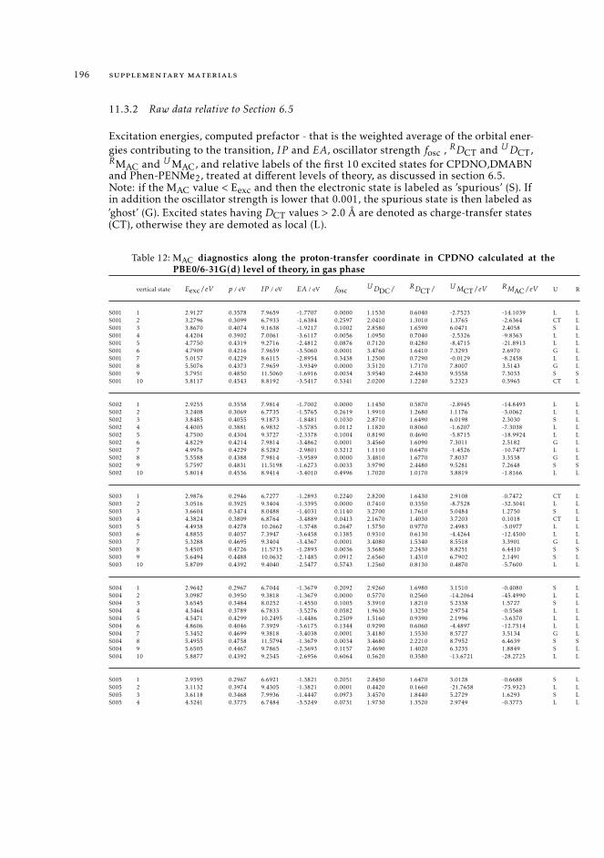
196 supplementary materials
11.3.2 Raw data relative to Section 6.5
Excitation energies, computed prefactor - that is the weighted average of the orbital ener-gies contributing to the transition, IP and EA, oscillator strength fosc , RDCT and UDCT,RMAC and UMAC, and relative labels of the first 10 excited states for CPDNO,DMABNand Phen-PENMe2, treated at different levels of theory, as discussed in section 6.5.Note: if the MAC value < Eexc and then the electronic state is labeled as ’spurious’ (S). Ifin addition the oscillator strength is lower that 0.001, the spurious state is then labeled as’ghost’ (G). Excited states having DCT values > 2.0 Å are denoted as charge-transfer states(CT), otherwise they are demoted as local (L).
Table 12: MAC diagnostics along the proton-transfer coordinate in CPDNO calculated at thePBE0/6-31G(d) level of theory, in gas phase
vertical state Eexc/eV p / eV IP / eV EA / eV fosc UDDC/ RDCT/ UMCT/eV RMAC/eV U R
S001 1 2.9127 0.3578 7.9659 -1.7707 0.0000 1.1530 0.6040 -2.7523 -14.1039 L LS001 2 3.2796 0.3099 6.7933 -1.6384 0.2597 2.0410 1.3010 1.3765 -2.6364 CT LS001 3 3.8670 0.4074 9.1638 -1.9217 0.1002 2.8580 1.6590 6.0471 2.4058 S LS001 4 4.4204 0.3902 7.0061 -3.6117 0.0056 1.0950 0.7040 -2.5326 -9.8363 L LS001 5 4.7750 0.4319 9.2716 -2.4812 0.0876 0.7120 0.4280 -8.4715 -21.8913 L LS001 6 4.7909 0.4216 7.9659 -3.5060 0.0001 3.4760 1.6410 7.3293 2.6970 G LS001 7 5.0157 0.4229 8.6115 -2.8954 0.3438 1.2500 0.7290 -0.0129 -8.2458 L LS001 8 5.5076 0.4373 7.9659 -3.9349 0.0000 3.5120 1.7170 7.8007 3.5143 G LS001 9 5.7951 0.4850 11.5060 -1.6916 0.0034 3.9540 2.4430 9.5558 7.3033 S SS001 10 5.8117 0.4543 8.8192 -3.5417 0.5341 2.0200 1.2240 5.2323 0.5965 CT L
S002 1 2.9255 0.3558 7.9814 -1.7002 0.0000 1.1450 0.5870 -2.8945 -14.8493 L LS002 2 3.2408 0.3069 6.7735 -1.5765 0.2619 1.9910 1.2680 1.1176 -3.0062 L LS002 3 3.8485 0.4055 9.1873 -1.8481 0.1030 2.8710 1.6490 6.0198 2.3030 S LS002 4 4.4005 0.3881 6.9832 -3.5785 0.0112 1.1820 0.8060 -1.6207 -7.3038 L LS002 5 4.7500 0.4304 9.3727 -2.3378 0.1004 0.8190 0.4690 -5.8715 -18.9924 L LS002 6 4.8229 0.4214 7.9814 -3.4862 0.0001 3.4560 1.6090 7.3011 2.5182 G LS002 7 4.9976 0.4229 8.5282 -2.9801 0.3212 1.1110 0.6470 -1.4526 -10.7477 L LS002 8 5.5588 0.4388 7.9814 -3.9589 0.0000 3.4810 1.6770 7.8037 3.3538 G LS002 9 5.7597 0.4831 11.5198 -1.6273 0.0033 3.9790 2.4480 9.5281 7.2648 S SS002 10 5.8014 0.4536 8.9414 -3.4010 0.4996 1.7020 1.0170 3.8819 -1.8166 L L
S003 1 2.9876 0.2946 6.7277 -1.2893 0.2240 2.8200 1.6430 2.9108 -0.7472 CT LS003 2 3.0516 0.3925 9.3404 -1.3395 0.0000 0.7410 0.3350 -8.7528 -32.3041 L LS003 3 3.6604 0.3474 8.0488 -1.4031 0.1140 3.2700 1.7610 5.0484 1.2750 S LS003 4 4.3824 0.3809 6.8764 -3.4889 0.0413 2.1670 1.4030 3.7203 0.1018 CT LS003 5 4.4938 0.4278 10.2662 -1.3748 0.2647 1.5750 0.9770 2.4983 -3.0977 L LS003 6 4.8855 0.4057 7.3947 -3.6458 0.1385 0.9310 0.6130 -4.4264 -12.4500 L LS003 7 5.3288 0.4695 9.3404 -3.4367 0.0001 3.4080 1.5340 8.5518 3.3901 G LS003 8 5.4505 0.4726 11.5715 -1.2893 0.0036 3.5680 2.2430 8.8251 6.4410 S SS003 9 5.6494 0.4488 10.0632 -2.1485 0.0912 2.6560 1.4310 6.7902 2.1491 S LS003 10 5.8709 0.4392 9.4040 -2.5477 0.5743 1.2560 0.8130 0.4870 -5.7600 L L
S004 1 2.9642 0.2967 6.7044 -1.3679 0.2092 2.9260 1.6980 3.1510 -0.4080 S LS004 2 3.0987 0.3950 9.3818 -1.3679 0.0000 0.5770 0.2560 -14.2064 -45.4990 L LS004 3 3.6545 0.3484 8.0252 -1.4550 0.1005 3.3910 1.8210 5.2338 1.5727 S LS004 4 4.3464 0.3789 6.7833 -3.5276 0.0582 1.9630 1.3250 2.9754 -0.5568 L LS004 5 4.5471 0.4299 10.2495 -1.4486 0.2509 1.5160 0.9390 2.1996 -3.6370 L LS004 6 4.8606 0.4046 7.3929 -3.6175 0.1344 0.9290 0.6060 -4.4897 -12.7514 L LS004 7 5.3452 0.4699 9.3818 -3.4038 0.0001 3.4180 1.5530 8.5727 3.5134 G LS004 8 5.4955 0.4758 11.5794 -1.3679 0.0034 3.4680 2.2210 8.7952 6.4639 S SS004 9 5.6505 0.4467 9.7865 -2.3693 0.1157 2.4690 1.4020 6.3235 1.8849 S LS004 10 5.8877 0.4392 9.2545 -2.6956 0.6064 0.5620 0.3580 -13.6721 -28.2725 L L
S005 1 2.9395 0.2967 6.6921 -1.3821 0.2051 2.8450 1.6470 3.0128 -0.6688 S LS005 2 3.1132 0.3974 9.4305 -1.3821 0.0001 0.4420 0.1660 -21.7658 -75.9323 L LS005 3 3.6118 0.3468 7.9936 -1.4447 0.0973 3.4570 1.8440 5.2729 1.6293 S LS005 4 4.3241 0.3775 6.7484 -3.5249 0.0731 1.9730 1.3520 2.9749 -0.3773 L L
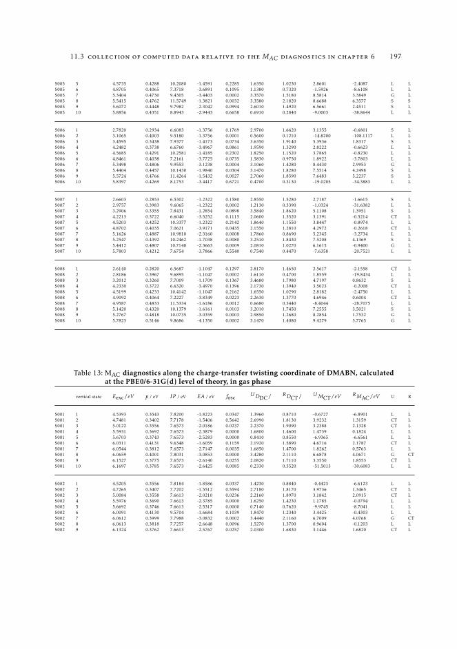
11.3 collection of computed data relative to the MAC diagnostics in chapter 6 197
S005 5 4.5735 0.4288 10.2080 -1.4591 0.2285 1.6350 1.0230 2.8601 -2.4087 L LS005 6 4.8705 0.4065 7.3718 -3.6891 0.1095 1.1380 0.7320 -1.5926 -8.6108 L LS005 7 5.3404 0.4730 9.4305 -3.4403 0.0002 3.3570 1.5180 8.5814 3.3849 G LS005 8 5.5415 0.4762 11.5749 -1.3821 0.0032 3.3580 2.1820 8.6688 6.3577 S SS005 9 5.6072 0.4448 9.7982 -2.3042 0.0994 2.6010 1.4920 6.5661 2.4511 S LS005 10 5.8856 0.4351 8.8943 -2.9443 0.6658 0.6910 0.2840 -9.0003 -38.8644 L L
S006 1 2.7820 0.2934 6.6083 -1.3756 0.1769 2.9700 1.6620 3.1355 -0.6801 S LS006 2 3.1065 0.4003 9.5180 -1.3756 0.0001 0.5600 0.1210 -14.8200 -108.1117 L LS006 3 3.4595 0.3438 7.9377 -1.4173 0.0734 3.6350 1.9140 5.3936 1.8317 S LS006 4 4.2482 0.3738 6.6760 -3.4967 0.0861 1.9590 1.3290 2.8222 -0.6623 L LS006 5 4.5685 0.4291 10.2581 -1.4185 0.2302 1.8250 1.1520 3.7865 -0.8230 L LS006 6 4.8461 0.4038 7.2161 -3.7725 0.0735 1.5830 0.9750 1.8922 -3.7803 L LS006 7 5.3498 0.4806 9.9553 -3.1238 0.0004 3.1060 1.4280 8.4430 2.9953 G LS006 8 5.4404 0.4457 10.1430 -1.9840 0.0304 3.1470 1.8280 7.5514 4.2498 S LS006 9 5.5724 0.4766 11.4264 -1.5432 0.0027 2.7060 1.8590 7.6483 5.2237 S LS006 10 5.8397 0.4269 8.1753 -3.4417 0.6721 0.4700 0.3130 -19.0205 -34.3883 L L
S007 1 2.6603 0.2853 6.5302 -1.2322 0.1580 2.8550 1.5280 2.7187 -1.6615 S LS007 2 2.9757 0.3983 9.6065 -1.2322 0.0002 1.2130 0.3390 -1.0324 -31.6382 L LS007 3 3.2906 0.3355 7.8431 -1.2854 0.0898 3.5840 1.8620 5.1108 1.3951 S LS007 4 4.2213 0.3722 6.6040 -3.5252 0.1115 2.0600 1.3520 3.1391 -0.5214 CT LS007 5 4.5203 0.4252 10.3377 -1.2322 0.2142 1.8640 1.1550 3.8447 -0.8974 L LS007 6 4.8702 0.4035 7.0621 -3.9171 0.0435 2.1550 1.2810 4.2972 -0.2618 CT LS007 7 5.1626 0.4887 10.9810 -2.3160 0.0008 1.7860 0.8690 5.2345 -3.2734 L LS007 8 5.2547 0.4392 10.2462 -1.7038 0.0080 3.2510 1.8430 7.5208 4.1369 S LS007 9 5.4412 0.4807 10.7148 -2.3663 0.0009 2.0810 1.0270 6.1615 -0.9400 G LS007 10 5.7803 0.4212 7.6754 -3.7866 0.5540 0.7540 0.4470 -7.6358 -20.7521 L L
S008 1 2.6140 0.2820 6.5687 -1.1047 0.1297 2.8170 1.4650 2.5617 -2.1558 CT LS008 2 2.8186 0.3967 9.6895 -1.1047 0.0002 1.6110 0.4700 1.8559 -19.8434 L LS008 3 3.2012 0.3260 7.7009 -1.1709 0.1367 3.4680 1.7980 4.7197 0.8632 S LS008 4 4.2330 0.3722 6.6320 -3.4970 0.1396 2.1730 1.3940 3.5023 -0.2008 CT LS008 5 4.5199 0.4233 10.4142 -1.1047 0.2162 1.6550 1.0290 2.8182 -2.4750 L LS008 6 4.9092 0.4064 7.2227 -3.8349 0.0223 2.2630 1.3770 4.6946 0.6004 CT LS008 7 4.9587 0.4833 11.5334 -1.6186 0.0012 0.6680 0.3440 -8.4044 -28.7075 L LS008 8 5.1420 0.4320 10.1379 -1.6161 0.0103 3.2010 1.7450 7.2555 3.5021 S LS008 9 5.2767 0.4818 10.0735 -3.0359 0.0003 2.9850 1.2680 8.2854 1.7532 G LS008 10 5.7823 0.5146 9.8686 -4.1350 0.0002 3.1470 1.4080 9.4279 3.7765 G L
Table 13: MAC diagnostics along the charge-transfer twisting coordinate of DMABN, calculatedat the PBE0/6-31G(d) level of theory, in gas phase
vertical state Eexc/eV p / eV IP / eV EA / eV fosc UDDC/ RDCT/ UMCT/eV RMAC/eV U R
S001 1 4.5393 0.3543 7.8200 -1.8223 0.0347 1.3960 0.8710 -0.6727 -6.8901 L LS001 2 4.7481 0.3402 7.7178 -1.5406 0.5642 2.6990 1.8130 3.9232 1.3159 CT LS001 3 5.0122 0.3556 7.6573 -2.0186 0.0237 2.2370 1.9090 3.2388 2.1328 CT LS001 4 5.5931 0.3692 7.6573 -2.3879 0.0000 1.6800 1.4600 1.4739 0.1824 L LS001 5 5.6703 0.3743 7.6573 -2.5283 0.0000 0.8410 0.8550 -6.9365 -6.6561 L LS001 6 6.0311 0.4131 9.6348 -1.6059 0.1159 2.1920 1.5890 4.6716 2.1787 CT LS001 7 6.0544 0.3812 7.6573 -2.7147 0.0035 1.6850 1.4700 1.8262 0.5763 L LS001 8 6.0659 0.4001 7.8031 -3.0853 0.0000 3.4280 2.1110 6.6878 4.0671 G CTS001 9 6.1527 0.3775 7.6573 -2.6140 0.0255 2.0820 1.7110 3.3550 1.8553 CT LS001 10 6.1697 0.3785 7.6573 -2.6425 0.0085 0.2330 0.3520 -51.5013 -30.6083 L L
S002 1 4.5205 0.3556 7.8184 -1.8586 0.0337 1.4230 0.8840 -0.4423 -6.6123 L LS002 2 4.7265 0.3407 7.7202 -1.5512 0.5594 2.7180 1.8170 3.9736 1.3465 CT LS002 3 5.0084 0.3558 7.6613 -2.0210 0.0236 2.2160 1.8970 3.1842 2.0915 CT LS002 4 5.5976 0.3690 7.6613 -2.3785 0.0000 1.6250 1.4230 1.1785 -0.0794 L LS002 5 5.6692 0.3746 7.6613 -2.5317 0.0000 0.7140 0.7620 -9.9745 -8.7041 L LS002 6 6.0091 0.4130 9.5704 -1.6684 0.1039 1.8470 1.2340 3.4425 -0.4303 L LS002 7 6.0612 0.3999 7.7988 -3.0832 0.0002 3.4440 2.1160 6.7009 4.0768 G CTS002 8 6.0613 0.3818 7.7257 -2.6648 0.0096 1.5270 1.3700 0.9604 -0.1203 L LS002 9 6.1324 0.3762 7.6613 -2.5767 0.0257 2.0300 1.6830 3.1446 1.6820 CT L
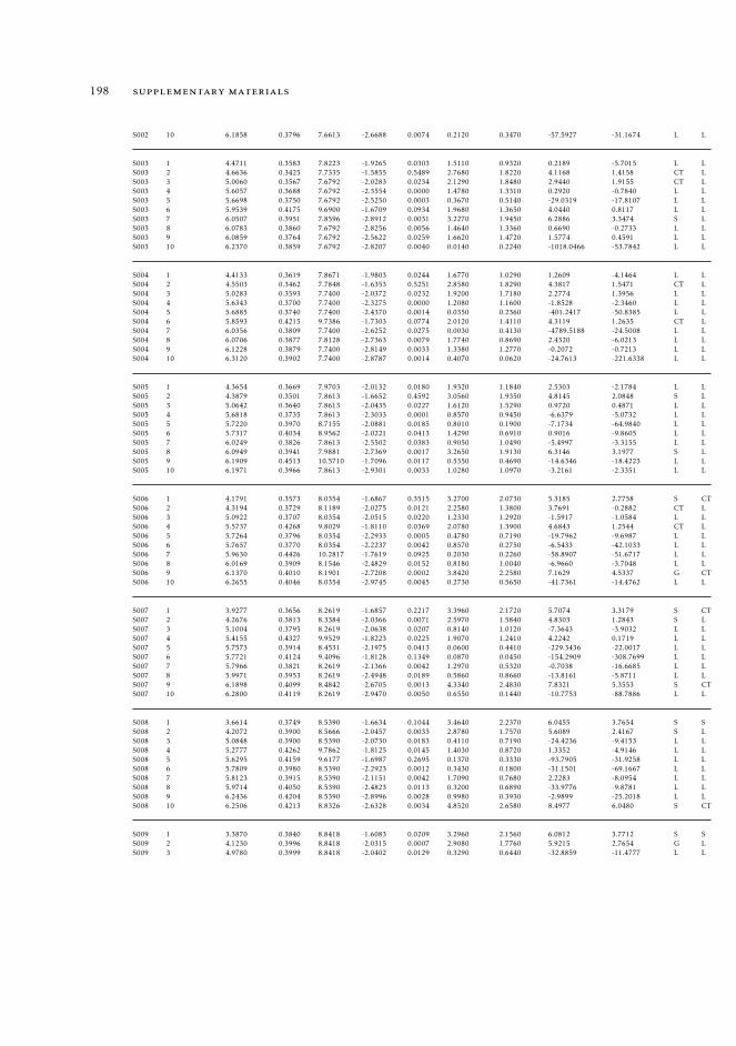
198 supplementary materials
S002 10 6.1858 0.3796 7.6613 -2.6688 0.0074 0.2120 0.3470 -57.5927 -31.1674 L L
S003 1 4.4711 0.3583 7.8223 -1.9265 0.0303 1.5110 0.9320 0.2189 -5.7015 L LS003 2 4.6636 0.3425 7.7335 -1.5855 0.5489 2.7680 1.8220 4.1168 1.4158 CT LS003 3 5.0060 0.3567 7.6792 -2.0283 0.0234 2.1290 1.8480 2.9440 1.9155 CT LS003 4 5.6057 0.3688 7.6792 -2.3554 0.0000 1.4780 1.3310 0.2920 -0.7840 L LS003 5 5.6698 0.3750 7.6792 -2.5250 0.0003 0.3670 0.5140 -29.0319 -17.8107 L LS003 6 5.9539 0.4175 9.6900 -1.6709 0.0934 1.9680 1.3650 4.0440 0.8117 L LS003 7 6.0507 0.3951 7.8596 -2.8912 0.0031 3.2270 1.9450 6.2886 3.3474 S LS003 8 6.0783 0.3860 7.6792 -2.8256 0.0056 1.4640 1.3360 0.6690 -0.2733 L LS003 9 6.0859 0.3764 7.6792 -2.5622 0.0259 1.6620 1.4720 1.5774 0.4591 L LS003 10 6.2370 0.3859 7.6792 -2.8207 0.0040 0.0140 0.2240 -1018.0466 -53.7842 L L
S004 1 4.4133 0.3619 7.8671 -1.9803 0.0244 1.6770 1.0290 1.2609 -4.1464 L LS004 2 4.5503 0.3462 7.7848 -1.6353 0.5251 2.8580 1.8290 4.3817 1.5471 CT LS004 3 5.0283 0.3593 7.7400 -2.0372 0.0232 1.9200 1.7180 2.2774 1.3956 L LS004 4 5.6343 0.3700 7.7400 -2.3275 0.0000 1.2080 1.1600 -1.8528 -2.3460 L LS004 5 5.6885 0.3740 7.7400 -2.4370 0.0014 0.0350 0.2360 -401.2417 -50.8385 L LS004 6 5.8593 0.4215 9.7386 -1.7303 0.0774 2.0120 1.4110 4.3119 1.2635 CT LS004 7 6.0356 0.3809 7.7400 -2.6252 0.0275 0.0030 0.4130 -4789.5188 -24.5008 L LS004 8 6.0706 0.3877 7.8128 -2.7363 0.0079 1.7740 0.8690 2.4320 -6.0213 L LS004 9 6.1228 0.3879 7.7400 -2.8149 0.0033 1.3380 1.2770 -0.2072 -0.7213 L LS004 10 6.3120 0.3902 7.7400 -2.8787 0.0014 0.4070 0.0620 -24.7613 -221.6338 L L
S005 1 4.3654 0.3669 7.9703 -2.0132 0.0180 1.9320 1.1840 2.5303 -2.1784 L LS005 2 4.3879 0.3501 7.8613 -1.6652 0.4592 3.0560 1.9350 4.8145 2.0848 S LS005 3 5.0642 0.3640 7.8613 -2.0435 0.0227 1.6120 1.5290 0.9720 0.4871 L LS005 4 5.6818 0.3735 7.8613 -2.3033 0.0001 0.8570 0.9450 -6.6379 -5.0732 L LS005 5 5.7220 0.3970 8.7155 -2.0881 0.0185 0.8010 0.1900 -7.1734 -64.9840 L LS005 6 5.7317 0.4034 8.9562 -2.0221 0.0413 1.4290 0.6910 0.9016 -9.8605 L LS005 7 6.0249 0.3826 7.8613 -2.5502 0.0383 0.9050 1.0490 -5.4997 -3.3155 L LS005 8 6.0949 0.3941 7.9881 -2.7369 0.0017 3.2650 1.9130 6.3146 3.1977 S LS005 9 6.1909 0.4513 10.5710 -1.7096 0.0117 0.5350 0.4690 -14.6346 -18.4223 L LS005 10 6.1971 0.3966 7.8613 -2.9301 0.0033 1.0280 1.0970 -3.2161 -2.3351 L L
S006 1 4.1791 0.3573 8.0354 -1.6867 0.3515 3.2700 2.0730 5.3185 2.7758 S CTS006 2 4.3194 0.3729 8.1189 -2.0275 0.0121 2.2580 1.3800 3.7691 -0.2882 CT LS006 3 5.0922 0.3707 8.0354 -2.0515 0.0220 1.2330 1.2920 -1.5917 -1.0584 L LS006 4 5.5737 0.4268 9.8029 -1.8110 0.0369 2.0780 1.3900 4.6843 1.2544 CT LS006 5 5.7264 0.3796 8.0354 -2.2933 0.0005 0.4780 0.7190 -19.7962 -9.6987 L LS006 6 5.7657 0.3770 8.0354 -2.2237 0.0042 0.8570 0.2750 -6.5433 -42.1033 L LS006 7 5.9630 0.4426 10.2817 -1.7619 0.0925 0.2030 0.2260 -58.8907 -51.6717 L LS006 8 6.0169 0.3909 8.1546 -2.4829 0.0152 0.8180 1.0040 -6.9660 -3.7048 L LS006 9 6.1370 0.4010 8.1901 -2.7208 0.0002 3.8420 2.2580 7.1629 4.5337 G CTS006 10 6.2655 0.4046 8.0354 -2.9745 0.0045 0.2730 0.5650 -41.7361 -14.4762 L L
S007 1 3.9277 0.3656 8.2619 -1.6857 0.2217 3.3960 2.1720 5.7074 3.3179 S CTS007 2 4.2676 0.3813 8.3384 -2.0366 0.0071 2.5970 1.5840 4.8303 1.2843 S LS007 3 5.1004 0.3795 8.2619 -2.0638 0.0207 0.8140 1.0120 -7.3643 -3.9032 L LS007 4 5.4155 0.4327 9.9529 -1.8223 0.0225 1.9070 1.2410 4.2242 0.1719 L LS007 5 5.7573 0.3914 8.4531 -2.1975 0.0413 0.0600 0.4410 -229.3436 -22.0017 L LS007 6 5.7721 0.4124 9.4096 -1.8128 0.1349 0.0870 0.0450 -154.2909 -308.7699 L LS007 7 5.7966 0.3821 8.2619 -2.1366 0.0042 1.2970 0.5320 -0.7038 -16.6685 L LS007 8 5.9971 0.3953 8.2619 -2.4948 0.0189 0.5860 0.8660 -13.8161 -5.8711 L LS007 9 6.1898 0.4099 8.4842 -2.6705 0.0013 4.3340 2.4830 7.8321 5.3553 S CTS007 10 6.2800 0.4119 8.2619 -2.9470 0.0050 0.6550 0.1440 -10.7753 -88.7886 L L
S008 1 3.6614 0.3749 8.5390 -1.6634 0.1044 3.4640 2.2370 6.0455 3.7654 S SS008 2 4.2072 0.3900 8.5666 -2.0457 0.0033 2.8780 1.7570 5.6089 2.4167 S LS008 3 5.0848 0.3900 8.5390 -2.0730 0.0183 0.4110 0.7190 -24.4236 -9.4153 L LS008 4 5.2777 0.4262 9.7862 -1.8125 0.0145 1.4030 0.8720 1.3352 -4.9146 L LS008 5 5.6295 0.4159 9.6177 -1.6987 0.2695 0.1370 0.3330 -93.7905 -31.9258 L LS008 6 5.7809 0.3980 8.5390 -2.2923 0.0012 0.3430 0.1800 -31.1501 -69.1667 L LS008 7 5.8123 0.3915 8.5390 -2.1151 0.0042 1.7090 0.7680 2.2283 -8.0954 L LS008 8 5.9714 0.4050 8.5390 -2.4823 0.0113 0.3200 0.6890 -33.9776 -9.8781 L LS008 9 6.2436 0.4204 8.5390 -2.8996 0.0028 0.9980 0.3930 -2.9899 -25.2018 L LS008 10 6.2506 0.4213 8.8326 -2.6328 0.0034 4.8520 2.6580 8.4977 6.0480 S CT
S009 1 3.3870 0.3840 8.8418 -1.6083 0.0209 3.2960 2.1560 6.0812 3.7712 S SS009 2 4.1230 0.3996 8.8418 -2.0315 0.0007 2.9080 1.7760 5.9215 2.7654 G LS009 3 4.9780 0.3999 8.8418 -2.0402 0.0129 0.3290 0.6440 -32.8859 -11.4777 L L
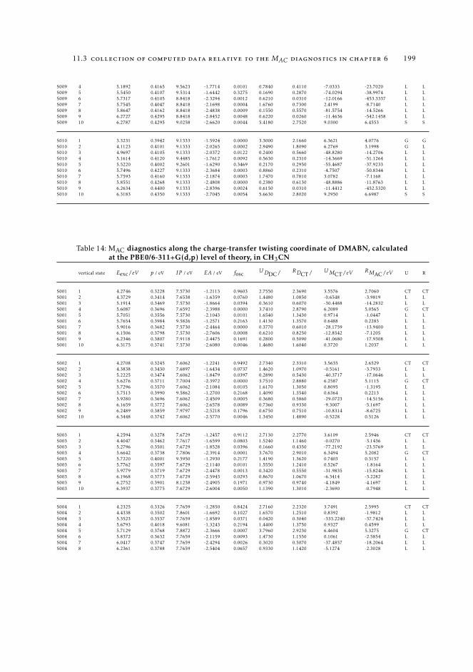
11.3 collection of computed data relative to the MAC diagnostics in chapter 6 199
S009 4 5.1892 0.4165 9.5623 -1.7714 0.0101 0.7840 0.4110 -7.0333 -23.7020 L LS009 5 5.5450 0.4107 9.5314 -1.6442 0.3275 0.1690 0.2870 -74.0294 -38.9974 L LS009 6 5.7317 0.4105 8.8418 -2.3294 0.0012 0.6210 0.0310 -12.0166 -453.3337 L LS009 7 5.7545 0.4047 8.8418 -2.1698 0.0004 1.6760 0.7300 2.4199 -8.7140 L LS009 8 5.8647 0.4162 8.8418 -2.4838 0.0009 0.1550 0.5570 -81.5754 -14.5266 L LS009 9 6.2727 0.4295 8.8418 -2.8452 0.0048 0.6220 0.0260 -11.4636 -542.1458 L LS009 10 6.2787 0.4295 9.0258 -2.6620 0.0044 5.4180 2.7520 9.0300 6.4553 S S
S010 1 3.3231 0.3942 9.1333 -1.5924 0.0000 3.3000 2.1660 6.3621 4.0776 G GS010 2 4.1123 0.4101 9.1333 -2.0265 0.0002 2.9490 1.8090 6.2769 3.1998 G LS010 3 4.9697 0.4105 9.1333 -2.0372 0.0122 0.2400 0.5660 -48.8280 -14.2706 L LS010 4 5.1614 0.4120 9.4485 -1.7612 0.0092 0.5630 0.2310 -14.3669 -51.1264 L LS010 5 5.5220 0.4002 9.2601 -1.6290 0.3469 0.2170 0.2950 -55.4687 -37.9233 L LS010 6 5.7496 0.4227 9.1333 -2.3684 0.0003 0.8860 0.2310 -4.7507 -50.8344 L LS010 7 5.7593 0.4160 9.1333 -2.1874 0.0003 1.7470 0.7810 3.0782 -7.1168 L LS010 8 5.8551 0.4268 9.1333 -2.4808 0.0000 0.2380 0.6130 -48.8886 -11.8763 L LS010 9 6.2634 0.4400 9.1333 -2.8396 0.0024 0.6150 0.0310 -11.4412 -452.5320 L LS010 10 6.3183 0.4350 9.1333 -2.7045 0.0054 5.6630 2.8020 9.2950 6.6987 S S
Table 14: MAC diagnostics along the charge-transfer twisting coordinate of DMABN, calculatedat the PBE0/6-311+G(d,p) level of theory, in CH3CN
vertical state Eexc/eV p / eV IP / eV EA / eV fosc UDDC/ RDCT/ UMCT/eV RMAC/eV U R
S001 1 4.2746 0.3228 7.5730 -1.2113 0.9603 2.7550 2.3690 3.5576 2.7060 CT CTS001 2 4.3729 0.3414 7.6538 -1.6359 0.0760 1.4480 1.0850 -0.6548 -3.9819 L LS001 3 5.1914 0.3469 7.5730 -1.8664 0.0394 0.3610 0.6070 -30.4488 -14.2832 L LS001 4 5.6087 0.3696 7.6592 -2.3988 0.0000 3.7410 2.8790 6.2089 5.0565 G CTS001 5 5.7051 0.3556 7.5730 -2.1043 0.0101 1.6540 1.3430 0.9714 -1.0447 L LS001 6 5.7654 0.3984 9.5826 -1.2571 0.2163 1.4130 1.3570 0.6488 0.2283 L LS001 7 5.9016 0.3682 7.5730 -2.4464 0.0000 0.3770 0.6010 -28.1759 -13.9400 L LS001 8 6.1506 0.3798 7.5730 -2.7606 0.0008 0.6210 0.8250 -12.8542 -7.1205 L LS001 9 6.2346 0.3807 7.9118 -2.4475 0.1691 0.2800 0.5090 -41.0680 -17.9308 L LS001 10 6.3175 0.3741 7.5730 -2.6080 0.0046 1.4680 1.6040 0.3720 1.2037 L L
S002 1 4.2708 0.3245 7.6062 -1.2241 0.9492 2.7340 2.3310 3.5635 2.6529 CT CTS002 2 4.3838 0.3430 7.6897 -1.6434 0.0737 1.4620 1.0970 -0.5161 -3.7933 L LS002 3 5.2225 0.3474 7.6062 -1.8479 0.0397 0.2890 0.5430 -40.3717 -17.0646 L LS002 4 5.6276 0.3711 7.7004 -2.3972 0.0000 3.7510 2.8880 6.2587 5.1115 G CTS002 5 5.7296 0.3570 7.6062 -2.1084 0.0105 1.6170 1.3050 0.8095 -1.3195 L LS002 6 5.7513 0.3990 9.5862 -1.2700 0.2168 1.4090 1.3540 0.6364 0.2213 L LS002 7 5.9280 0.3696 7.6062 -2.4509 0.0005 0.3680 0.5860 -29.0723 -14.5156 L LS002 8 6.1659 0.3772 7.6062 -2.6578 0.0089 0.7360 0.9330 -9.3007 -5.1697 L LS002 9 6.2489 0.3859 7.9797 -2.5218 0.1796 0.6750 0.7510 -10.8314 -8.6725 L LS002 10 6.3448 0.3742 7.6062 -2.5770 0.0046 1.3450 1.4890 -0.5228 0.5126 L L
S003 1 4.2594 0.3278 7.6729 -1.2457 0.9112 2.7130 2.2770 3.6109 2.5946 CT CTS003 2 4.4047 0.3462 7.7617 -1.6599 0.0803 1.5240 1.1460 -0.0270 -3.1436 L LS003 3 5.2796 0.3501 7.6729 -1.8528 0.0396 0.1660 0.4350 -77.2192 -23.5769 L LS003 4 5.6642 0.3738 7.7806 -2.3914 0.0001 3.7670 2.9010 6.3494 5.2082 G CTS003 5 5.7220 0.4001 9.5950 -1.2930 0.2177 1.4190 1.3620 0.7403 0.3157 L LS003 6 5.7762 0.3597 7.6729 -2.1140 0.0101 1.5550 1.2410 0.5267 -1.8164 L LS003 7 5.9779 0.3719 7.6729 -2.4478 0.0013 0.3420 0.5550 -31.9835 -15.8246 L LS003 8 6.1968 0.3773 7.6729 -2.5943 0.0293 0.8670 1.0670 -6.3414 -3.2282 L LS003 9 6.2752 0.3901 8.1238 -2.4905 0.1971 0.9730 0.9740 -4.1849 -4.1697 L LS003 10 6.3937 0.3775 7.6729 -2.6004 0.0050 1.1390 1.3010 -2.3690 -0.7948 L L
S004 1 4.2325 0.3326 7.7659 -1.2850 0.8424 2.7160 2.2320 3.7491 2.5995 CT CTS004 2 4.4338 0.3502 7.8601 -1.6692 0.1027 1.6570 1.2510 0.8392 -1.9812 L LS004 3 5.3523 0.3537 7.7659 -1.8589 0.0371 0.0420 0.3040 -333.2240 -37.7424 L LS004 4 5.6793 0.4018 9.6081 -1.3243 0.2194 1.4400 1.3750 0.9327 0.4599 L LS004 5 5.7129 0.3768 7.8872 -2.3666 0.0007 3.7960 2.9230 6.4604 5.3275 G CTS004 6 5.8372 0.3632 7.7659 -2.1159 0.0093 1.4730 1.1550 0.1061 -2.5854 L LS004 7 6.0417 0.3747 7.7659 -2.4294 0.0026 0.3020 0.5070 -37.4857 -18.2064 L LS004 8 6.2361 0.3788 7.7659 -2.5404 0.0657 0.9330 1.1420 -5.1274 -2.3028 L L
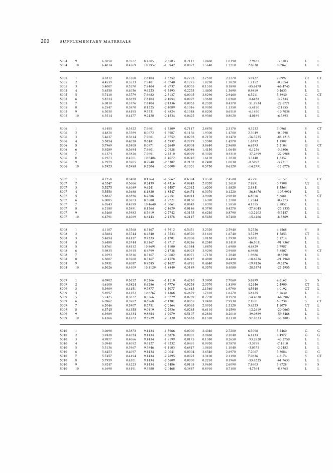
200 supplementary materials
S004 9 6.3050 0.3977 8.4705 -2.3503 0.2117 1.0460 1.0190 -2.9455 -3.3103 L LS004 10 6.4014 0.4369 10.2957 -1.5942 0.0072 1.5640 1.2210 2.6830 0.0967 L L
S005 1 4.1812 0.3368 7.8404 -1.3252 0.7725 2.7570 2.2270 3.9427 2.6997 CT CTS005 2 4.4539 0.3533 7.9401 -1.6740 0.1275 1.8230 1.3820 1.7152 -0.8054 L LS005 3 5.4007 0.3570 7.8404 -1.8737 0.0335 0.1510 0.1890 -85.6478 -66.4745 L LS005 4 5.6358 0.4036 9.6223 -1.3593 0.2253 1.4400 1.3690 0.9819 0.4633 L LS005 5 5.7418 0.3779 7.9682 -2.3137 0.0005 3.8290 2.9460 6.5211 5.3940 G CTS005 6 5.8734 0.3655 7.8404 -2.1054 0.0097 1.3630 1.0360 -0.6188 -3.9534 L LS005 7 6.0810 0.3776 7.8404 -2.4336 0.0055 0.2320 0.4370 -51.7934 -22.6771 L LS005 8 6.2547 0.3870 8.1225 -2.4089 0.1016 0.9030 1.1350 -5.4150 -2.1555 L LS005 9 6.3030 0.4195 9.5331 -1.8824 0.1348 0.8200 0.6510 -6.1450 -10.7038 L LS005 10 6.3514 0.4177 9.2420 -2.1234 0.0422 0.9360 0.8020 -4.0189 -6.5893 L L
S006 1 4.1455 0.3422 7.9601 -1.3509 0.7117 2.8870 2.3170 4.3232 3.0961 S CTS006 2 4.4820 0.3589 8.0672 -1.6987 0.1136 1.9300 1.4700 2.3049 -0.0298 L LS006 3 5.4637 0.3614 7.9601 -1.8752 0.0293 0.2170 0.1470 -56.5225 -88.1215 L LS006 4 5.5854 0.4058 9.6481 -1.3937 0.2279 1.5380 1.4570 1.6792 1.1587 L LS006 5 5.7969 0.3808 8.0971 -2.2649 0.0008 3.8680 2.9680 6.6393 5.5104 G CTS006 6 5.9289 0.3694 7.9601 -2.0928 0.0086 1.4150 1.0640 -0.1236 -3.4806 L LS006 7 6.1374 0.3826 7.9601 -2.4510 0.0099 0.3020 0.4310 -37.2699 -22.9988 L LS006 8 6.1973 0.4501 10.8404 -1.4072 0.0242 1.6120 1.3830 3.3148 1.8357 L LS006 9 6.2979 0.3905 8.2948 -2.3307 0.2132 0.7490 1.0030 -8.5997 -3.7311 L LS006 10 6.3923 0.3988 8.2504 -2.6008 0.1051 0.5730 0.6120 -14.2791 -12.6776 L L
S007 1 4.1258 0.3488 8.1264 -1.3662 0.6384 3.0550 2.4500 4.7791 3.6152 S CTS007 2 4.5247 0.3666 8.2439 -1.7316 0.0843 2.0320 1.5610 2.8891 0.7509 CT LS007 3 5.5275 0.4069 9.6241 -1.4487 0.2012 1.6200 1.4820 2.1841 1.3564 L LS007 4 5.5550 0.3688 8.1820 -1.8547 0.0474 0.3070 0.1220 -36.8676 -107.9931 L LS007 5 5.8827 0.3856 8.2786 -2.2151 0.0014 3.9000 2.9840 6.8016 5.6681 S CTS007 6 6.0085 0.3873 8.5680 -1.9721 0.0150 1.6390 1.2780 1.7544 -0.7273 L LS007 7 6.0543 0.4399 10.4640 -1.5061 0.0643 1.8370 1.5850 4.1315 2.8852 L LS007 8 6.2180 0.3891 8.1264 -2.4629 0.0146 0.3790 0.4270 -27.4045 -23.1335 L LS007 9 6.3468 0.3982 8.5619 -2.2742 0.3155 0.6240 0.8790 -12.2402 -5.5457 L LS007 10 6.4791 0.4069 8.6443 -2.4278 0.2117 0.5430 0.7400 -15.4466 -8.3869 L L
S008 1 4.1107 0.3568 8.3167 -1.3912 0.5451 3.2320 2.5940 5.2526 4.1568 S SS008 2 4.5684 0.3744 8.4340 -1.7533 0.0520 2.1610 1.6740 3.5239 1.5853 CT LS008 3 5.4654 0.4117 9.7323 -1.4701 0.2006 1.9130 1.7930 3.6751 3.1714 L LS008 4 5.6488 0.3744 8.3167 -1.8717 0.0246 0.2540 0.1410 -46.5031 -91.9367 L LS008 5 5.8761 0.4512 10.8691 -1.4100 0.1544 1.8470 1.6980 4.4829 3.7987 L LS008 6 5.9835 0.3915 8.4799 -2.1738 0.0023 3.9290 2.9980 6.9888 5.8507 S CTS008 7 6.1093 0.3816 8.3167 -2.0682 0.0071 1.7150 1.2840 1.9886 -0.8298 L LS008 8 6.3007 0.3960 8.3167 -2.4578 0.0217 0.4890 0.4490 -18.6726 -21.2960 L LS008 9 6.3931 0.4087 8.9585 -2.1627 0.4781 0.4640 0.6920 -19.9126 -9.6876 L LS008 10 6.5026 0.4409 10.1129 -1.8849 0.3189 0.3570 0.4080 -28.3374 -23.2955 L L
S009 1 4.0902 0.3652 8.5266 -1.4110 0.4210 3.3900 2.7060 5.6899 4.6162 S SS009 2 4.6108 0.3824 8.6286 -1.7776 0.0258 2.3370 1.8190 4.2446 2.4900 CT LS009 3 5.3909 0.4151 9.7877 -1.5077 0.1613 2.1360 1.9790 4.5540 4.0192 CT LS009 4 5.6957 0.4452 10.6767 -1.4368 0.2679 1.7410 1.6270 3.8425 3.2630 L LS009 5 5.7425 0.3822 8.5266 -1.8729 0.0289 0.2220 0.1920 -54.4638 -64.5987 L LS009 6 6.0967 0.3982 8.6968 -2.1381 0.0035 3.9410 2.9930 7.1811 6.0238 S CTS009 7 6.2046 0.3907 8.5751 -2.0564 0.0065 2.0010 1.5120 3.4353 1.1079 CT LS009 8 6.3745 0.4155 9.0119 -2.2936 0.0265 0.6110 0.4590 -12.2619 -20.0663 L LS009 9 6.3989 0.4334 9.8854 -1.9079 0.5107 0.2830 0.2010 -39.0889 -59.8468 L LS009 10 6.4266 0.4272 9.5929 -2.0320 0.5685 0.1320 0.3130 -97.4633 -34.3803 L L
S010 1 3.0698 0.3873 9.1434 -1.3966 0.0000 3.4040 2.7200 6.3098 5.2460 G GS010 2 3.9428 0.4054 9.1434 -1.8878 0.0001 2.9460 2.2040 6.1433 4.4977 G GS010 3 4.9877 0.4066 9.1434 -1.9199 0.0175 0.1380 0.2650 -93.2820 -43.2750 L LS010 4 5.0940 0.4092 9.6127 -1.5232 0.0491 0.9920 0.7870 -3.3799 -7.1610 L LS010 5 5.3136 0.3967 9.3846 -1.4103 0.6817 1.0410 1.1040 -3.0375 -2.2482 L LS010 6 5.6453 0.4097 9.1434 -2.0041 0.0004 3.6540 2.6970 7.2067 5.8084 G GS010 7 5.7457 0.4194 9.1434 -2.2695 0.0022 3.3100 2.1190 7.0626 4.6174 S CTS010 8 5.7959 0.4301 9.1434 -2.5609 0.0000 0.2210 0.1960 -53.4525 -61.7633 L LS010 9 5.9247 0.4223 9.1434 -2.3486 0.0105 3.9650 2.6090 7.8603 5.9728 S SS010 10 6.1698 0.4191 9.3580 -2.0468 0.3847 0.8910 0.7100 -4.7564 -8.8763 L L
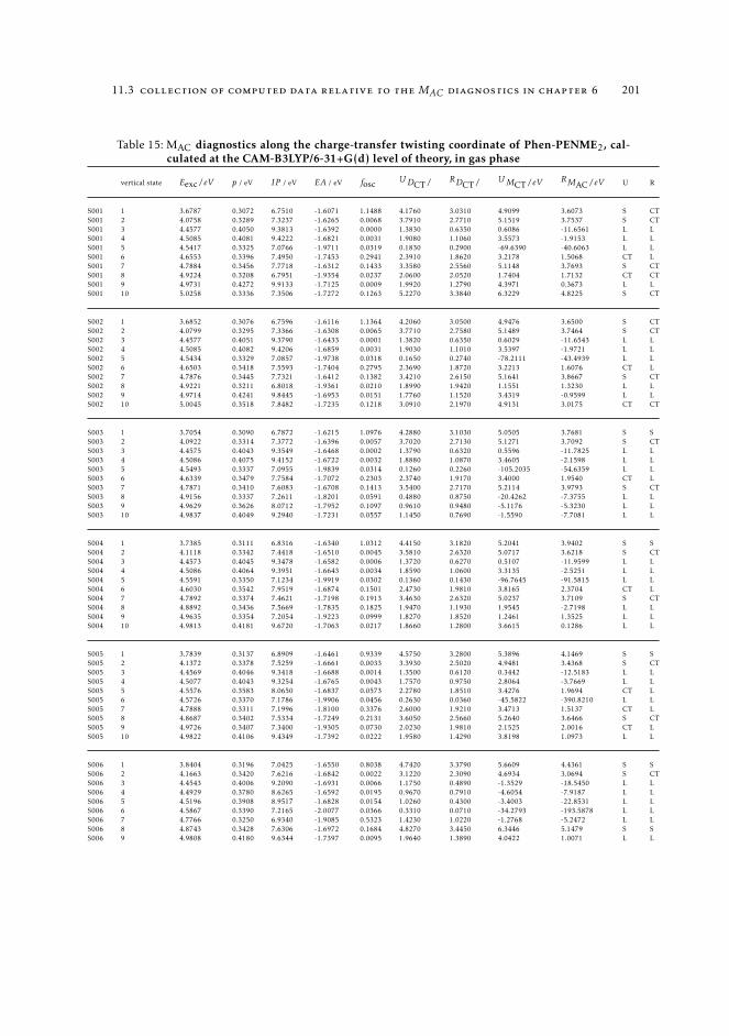
11.3 collection of computed data relative to the MAC diagnostics in chapter 6 201
Table 15: MAC diagnostics along the charge-transfer twisting coordinate of Phen-PENME2, cal-culated at the CAM-B3LYP/6-31+G(d) level of theory, in gas phase
vertical state Eexc/eV p / eV IP / eV EA / eV fosc UDCT/ RDCT/ UMCT/eV RMAC/eV U R
S001 1 3.6787 0.3072 6.7510 -1.6071 1.1488 4.1760 3.0310 4.9099 3.6073 S CTS001 2 4.0758 0.3289 7.3237 -1.6265 0.0068 3.7910 2.7710 5.1519 3.7537 S CTS001 3 4.4577 0.4050 9.3813 -1.6392 0.0000 1.3830 0.6350 0.6086 -11.6561 L LS001 4 4.5085 0.4081 9.4222 -1.6821 0.0031 1.9080 1.1060 3.5573 -1.9153 L LS001 5 4.5417 0.3325 7.0766 -1.9711 0.0319 0.1830 0.2900 -69.6390 -40.6063 L LS001 6 4.6553 0.3396 7.4950 -1.7453 0.2941 2.3910 1.8620 3.2178 1.5068 CT LS001 7 4.7884 0.3456 7.7718 -1.6312 0.1433 3.3580 2.5560 5.1148 3.7693 S CTS001 8 4.9224 0.3208 6.7951 -1.9354 0.0237 2.0600 2.0520 1.7404 1.7132 CT CTS001 9 4.9731 0.4272 9.9133 -1.7125 0.0009 1.9920 1.2790 4.3971 0.3673 L LS001 10 5.0258 0.3336 7.3506 -1.7272 0.1263 5.2270 3.3840 6.3229 4.8225 S CT
S002 1 3.6852 0.3076 6.7596 -1.6116 1.1364 4.2060 3.0500 4.9476 3.6500 S CTS002 2 4.0799 0.3295 7.3366 -1.6308 0.0065 3.7710 2.7580 5.1489 3.7464 S CTS002 3 4.4577 0.4051 9.3790 -1.6433 0.0001 1.3820 0.6350 0.6029 -11.6543 L LS002 4 4.5085 0.4082 9.4206 -1.6859 0.0031 1.9030 1.1010 3.5397 -1.9721 L LS002 5 4.5434 0.3329 7.0857 -1.9738 0.0318 0.1650 0.2740 -78.2111 -43.4939 L LS002 6 4.6503 0.3418 7.5593 -1.7404 0.2795 2.3690 1.8720 3.2213 1.6076 CT LS002 7 4.7876 0.3445 7.7321 -1.6412 0.1382 3.4210 2.6150 5.1641 3.8667 S CTS002 8 4.9221 0.3211 6.8018 -1.9361 0.0210 1.8990 1.9420 1.1551 1.3230 L LS002 9 4.9714 0.4241 9.8445 -1.6953 0.0151 1.7760 1.1520 3.4319 -0.9599 L LS002 10 5.0045 0.3518 7.8482 -1.7235 0.1218 3.0910 2.1970 4.9131 3.0175 CT CT
S003 1 3.7054 0.3090 6.7872 -1.6215 1.0976 4.2880 3.1030 5.0505 3.7681 S SS003 2 4.0922 0.3314 7.3772 -1.6396 0.0057 3.7020 2.7130 5.1271 3.7092 S CTS003 3 4.4575 0.4043 9.3549 -1.6468 0.0002 1.3790 0.6320 0.5596 -11.7825 L LS003 4 4.5086 0.4075 9.4152 -1.6722 0.0032 1.8880 1.0870 3.4605 -2.1598 L LS003 5 4.5493 0.3337 7.0955 -1.9839 0.0314 0.1260 0.2260 -105.2035 -54.6359 L LS003 6 4.6339 0.3479 7.7584 -1.7072 0.2303 2.3740 1.9170 3.4000 1.9540 CT LS003 7 4.7871 0.3410 7.6083 -1.6708 0.1413 3.5400 2.7170 5.2114 3.9793 S CTS003 8 4.9156 0.3337 7.2611 -1.8201 0.0591 0.4880 0.8750 -20.4262 -7.3755 L LS003 9 4.9629 0.3626 8.0712 -1.7952 0.1097 0.9610 0.9480 -5.1176 -5.3230 L LS003 10 4.9837 0.4049 9.2940 -1.7231 0.0557 1.1450 0.7690 -1.5590 -7.7081 L L
S004 1 3.7385 0.3111 6.8316 -1.6340 1.0312 4.4150 3.1820 5.2041 3.9402 S SS004 2 4.1118 0.3342 7.4418 -1.6510 0.0045 3.5810 2.6320 5.0717 3.6218 S CTS004 3 4.4573 0.4045 9.3478 -1.6582 0.0006 1.3720 0.6270 0.5107 -11.9599 L LS004 4 4.5086 0.4064 9.3951 -1.6643 0.0034 1.8590 1.0600 3.3135 -2.5251 L LS004 5 4.5591 0.3350 7.1234 -1.9919 0.0302 0.1360 0.1430 -96.7645 -91.5815 L LS004 6 4.6030 0.3542 7.9519 -1.6874 0.1501 2.4730 1.9810 3.8165 2.3704 CT LS004 7 4.7892 0.3374 7.4621 -1.7198 0.1913 3.4630 2.6320 5.0237 3.7109 S CTS004 8 4.8892 0.3436 7.5669 -1.7835 0.1825 1.9470 1.1930 1.9545 -2.7198 L LS004 9 4.9635 0.3354 7.2054 -1.9223 0.0999 1.8270 1.8520 1.2461 1.3525 L LS004 10 4.9813 0.4181 9.6720 -1.7063 0.0217 1.8660 1.2800 3.6615 0.1286 L L
S005 1 3.7839 0.3137 6.8909 -1.6461 0.9339 4.5750 3.2800 5.3896 4.1469 S SS005 2 4.1372 0.3378 7.5259 -1.6661 0.0033 3.3930 2.5020 4.9481 3.4368 S CTS005 3 4.4569 0.4046 9.3418 -1.6688 0.0014 1.3500 0.6120 0.3442 -12.5183 L LS005 4 4.5077 0.4043 9.3254 -1.6765 0.0043 1.7570 0.9750 2.8064 -3.7669 L LS005 5 4.5576 0.3583 8.0650 -1.6837 0.0573 2.2780 1.8510 3.4276 1.9694 CT LS005 6 4.5726 0.3370 7.1786 -1.9906 0.0456 0.2630 0.0360 -45.5822 -390.8210 L LS005 7 4.7888 0.3311 7.1996 -1.8100 0.3376 2.6000 1.9210 3.4713 1.5137 CT LS005 8 4.8687 0.3402 7.5334 -1.7249 0.2131 3.6050 2.5660 5.2640 3.6466 S CTS005 9 4.9726 0.3407 7.3400 -1.9305 0.0730 2.0230 1.9810 2.1525 2.0016 CT LS005 10 4.9822 0.4106 9.4349 -1.7392 0.0222 1.9580 1.4290 3.8198 1.0973 L L
S006 1 3.8404 0.3196 7.0425 -1.6550 0.8038 4.7420 3.3790 5.6609 4.4361 S SS006 2 4.1663 0.3420 7.6216 -1.6842 0.0022 3.1220 2.3090 4.6934 3.0694 S CTS006 3 4.4543 0.4006 9.2090 -1.6931 0.0066 1.1750 0.4890 -1.3529 -18.5450 L LS006 4 4.4929 0.3780 8.6265 -1.6592 0.0195 0.9670 0.7910 -4.6054 -7.9187 L LS006 5 4.5196 0.3908 8.9517 -1.6828 0.0154 1.0260 0.4300 -3.4003 -22.8531 L LS006 6 4.5867 0.3390 7.2165 -2.0077 0.0366 0.3310 0.0710 -34.2793 -193.5878 L LS006 7 4.7766 0.3250 6.9340 -1.9085 0.5323 1.4230 1.0220 -1.2768 -5.2472 L LS006 8 4.8743 0.3428 7.6306 -1.6972 0.1684 4.8270 3.4450 6.3446 5.1479 S SS006 9 4.9808 0.4180 9.6344 -1.7397 0.0095 1.9640 1.3890 4.0422 1.0071 L L
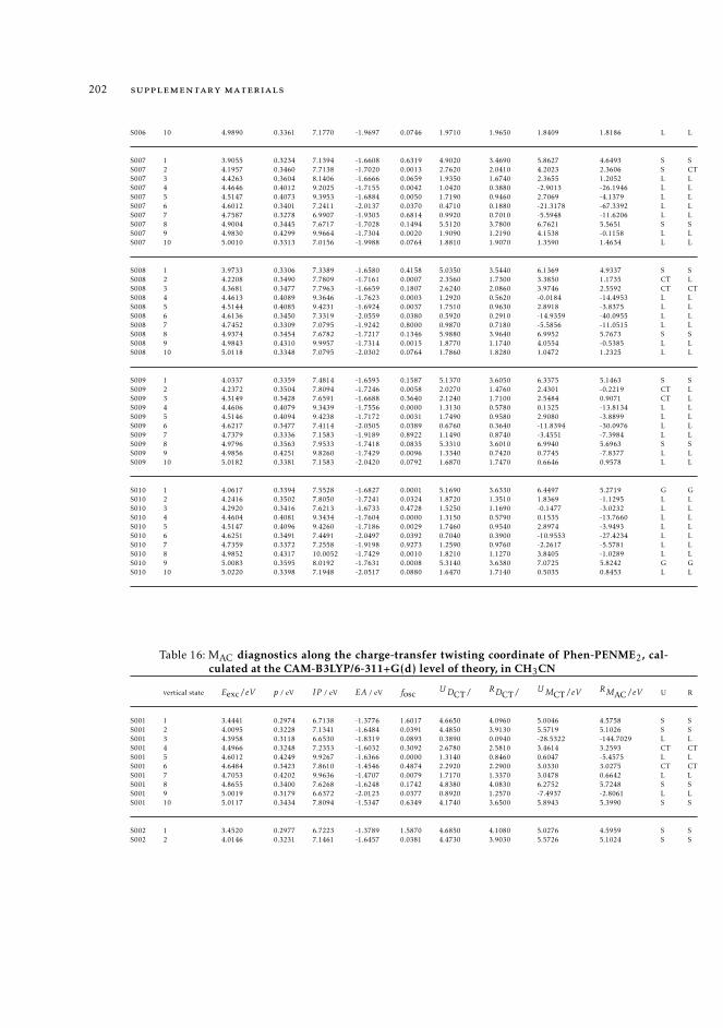
202 supplementary materials
S006 10 4.9890 0.3361 7.1770 -1.9697 0.0746 1.9710 1.9650 1.8409 1.8186 L L
S007 1 3.9055 0.3234 7.1394 -1.6608 0.6319 4.9020 3.4690 5.8627 4.6493 S SS007 2 4.1957 0.3460 7.7138 -1.7020 0.0013 2.7620 2.0410 4.2023 2.3606 S CTS007 3 4.4263 0.3604 8.1406 -1.6666 0.0659 1.9350 1.6740 2.3655 1.2052 L LS007 4 4.4646 0.4012 9.2025 -1.7155 0.0042 1.0420 0.3880 -2.9013 -26.1946 L LS007 5 4.5147 0.4073 9.3953 -1.6884 0.0050 1.7190 0.9460 2.7069 -4.1379 L LS007 6 4.6012 0.3401 7.2411 -2.0137 0.0370 0.4710 0.1880 -21.3178 -67.3392 L LS007 7 4.7587 0.3278 6.9907 -1.9303 0.6814 0.9920 0.7010 -5.5948 -11.6206 L LS007 8 4.9004 0.3445 7.6717 -1.7028 0.1494 5.5120 3.7800 6.7621 5.5651 S SS007 9 4.9830 0.4299 9.9664 -1.7304 0.0020 1.9090 1.2190 4.1538 -0.1158 L LS007 10 5.0010 0.3313 7.0156 -1.9988 0.0764 1.8810 1.9070 1.3590 1.4634 L L
S008 1 3.9733 0.3306 7.3389 -1.6580 0.4158 5.0350 3.5440 6.1369 4.9337 S SS008 2 4.2208 0.3490 7.7809 -1.7161 0.0007 2.3560 1.7300 3.3850 1.1735 CT LS008 3 4.3681 0.3477 7.7963 -1.6659 0.1807 2.6240 2.0860 3.9746 2.5592 CT CTS008 4 4.4613 0.4089 9.3646 -1.7623 0.0003 1.2920 0.5620 -0.0184 -14.4953 L LS008 5 4.5144 0.4085 9.4231 -1.6924 0.0037 1.7510 0.9630 2.8918 -3.8375 L LS008 6 4.6136 0.3450 7.3319 -2.0559 0.0380 0.5920 0.2910 -14.9359 -40.0955 L LS008 7 4.7452 0.3309 7.0795 -1.9242 0.8000 0.9870 0.7180 -5.5856 -11.0515 L LS008 8 4.9374 0.3454 7.6782 -1.7217 0.1346 5.9880 3.9640 6.9952 5.7673 S SS008 9 4.9843 0.4310 9.9957 -1.7314 0.0015 1.8770 1.1740 4.0554 -0.5385 L LS008 10 5.0118 0.3348 7.0795 -2.0302 0.0764 1.7860 1.8280 1.0472 1.2325 L L
S009 1 4.0337 0.3359 7.4814 -1.6593 0.1587 5.1370 3.6050 6.3375 5.1463 S SS009 2 4.2372 0.3504 7.8094 -1.7246 0.0058 2.0270 1.4760 2.4301 -0.2219 CT LS009 3 4.3149 0.3428 7.6591 -1.6688 0.3640 2.1240 1.7100 2.5484 0.9071 CT LS009 4 4.4606 0.4079 9.3439 -1.7556 0.0000 1.3130 0.5780 0.1325 -13.8134 L LS009 5 4.5146 0.4094 9.4238 -1.7172 0.0031 1.7490 0.9580 2.9080 -3.8899 L LS009 6 4.6217 0.3477 7.4114 -2.0505 0.0389 0.6760 0.3640 -11.8394 -30.0976 L LS009 7 4.7379 0.3336 7.1583 -1.9189 0.8922 1.1490 0.8740 -3.4551 -7.3984 L LS009 8 4.9796 0.3563 7.9533 -1.7418 0.0835 5.3310 3.6010 6.9940 5.6963 S SS009 9 4.9856 0.4251 9.8260 -1.7429 0.0096 1.3340 0.7420 0.7745 -7.8377 L LS009 10 5.0182 0.3381 7.1583 -2.0420 0.0792 1.6870 1.7470 0.6646 0.9578 L L
S010 1 4.0617 0.3394 7.5528 -1.6827 0.0001 5.1690 3.6330 6.4497 5.2719 G GS010 2 4.2416 0.3502 7.8050 -1.7241 0.0324 1.8720 1.3510 1.8369 -1.1295 L LS010 3 4.2920 0.3416 7.6213 -1.6733 0.4728 1.5250 1.1690 -0.1477 -3.0232 L LS010 4 4.4604 0.4081 9.3434 -1.7604 0.0000 1.3150 0.5790 0.1535 -13.7660 L LS010 5 4.5147 0.4096 9.4260 -1.7186 0.0029 1.7460 0.9540 2.8974 -3.9493 L LS010 6 4.6251 0.3491 7.4491 -2.0497 0.0392 0.7040 0.3900 -10.9553 -27.4234 L LS010 7 4.7359 0.3372 7.2558 -1.9198 0.9273 1.2590 0.9760 -2.2617 -5.5781 L LS010 8 4.9852 0.4317 10.0052 -1.7429 0.0010 1.8210 1.1270 3.8405 -1.0289 L LS010 9 5.0083 0.3595 8.0192 -1.7631 0.0008 5.3140 3.6380 7.0725 5.8242 G GS010 10 5.0220 0.3398 7.1948 -2.0517 0.0880 1.6470 1.7140 0.5035 0.8453 L L
Table 16: MAC diagnostics along the charge-transfer twisting coordinate of Phen-PENME2, cal-culated at the CAM-B3LYP/6-311+G(d) level of theory, in CH3CN
vertical state Eexc/eV p / eV IP / eV EA / eV fosc UDCT/ RDCT/ UMCT/eV RMAC/eV U R
S001 1 3.4441 0.2974 6.7138 -1.3776 1.6017 4.6650 4.0960 5.0046 4.5758 S SS001 2 4.0095 0.3228 7.1341 -1.6484 0.0391 4.4850 3.9130 5.5719 5.1026 S SS001 3 4.3958 0.3118 6.6530 -1.8319 0.0893 0.3890 0.0940 -28.5322 -144.7029 L LS001 4 4.4966 0.3248 7.2353 -1.6032 0.3092 2.6780 2.5810 3.4614 3.2593 CT CTS001 5 4.6012 0.4249 9.9267 -1.6366 0.0000 1.3140 0.8460 0.6047 -5.4575 L LS001 6 4.6484 0.3423 7.8610 -1.4546 0.4874 2.2920 2.2900 3.0330 3.0275 CT CTS001 7 4.7053 0.4202 9.9636 -1.4707 0.0079 1.7170 1.3370 3.0478 0.6642 L LS001 8 4.8655 0.3400 7.6268 -1.6248 0.1742 4.8380 4.0830 6.2752 5.7248 S SS001 9 5.0019 0.3179 6.6372 -2.0123 0.0377 0.8920 1.2570 -7.4937 -2.8061 L LS001 10 5.0117 0.3434 7.8094 -1.5347 0.6349 4.1740 3.6500 5.8943 5.3990 S S
S002 1 3.4520 0.2977 6.7223 -1.3789 1.5870 4.6850 4.1080 5.0276 4.5959 S SS002 2 4.0146 0.3231 7.1461 -1.6457 0.0381 4.4730 3.9030 5.5726 5.1024 S S
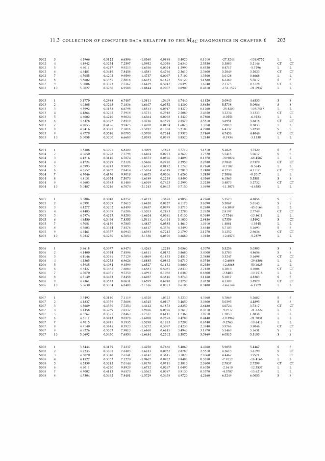
11.3 collection of computed data relative to the MAC diagnostics in chapter 6 203
S002 3 4.3966 0.3122 6.6596 -1.8360 0.0898 0.4020 0.1010 -27.3244 -134.0752 L LS002 4 4.4942 0.3254 7.2597 -1.5952 0.3058 2.6340 2.5530 3.3880 3.2146 CT CTS002 5 4.6011 0.4247 9.9213 -1.6356 0.0024 1.2990 0.8330 0.4717 -5.7296 L LS002 6 4.6481 0.3419 7.8458 -1.4581 0.4796 2.3610 2.3600 3.2049 3.2023 CT CTS002 7 4.7055 0.4202 9.9599 -1.4737 0.0097 1.7100 1.3300 3.0128 0.6068 L LS002 8 4.8602 0.3381 7.5816 -1.6184 0.1623 5.0120 4.1880 6.3269 5.7617 S SS002 9 5.0006 0.3373 7.5367 -1.6429 0.5042 2.0390 1.6240 2.1175 0.3128 CT LS002 10 5.0027 0.3250 6.9588 -1.8844 0.2007 0.0900 0.4810 -151.1529 -21.0937 L L
S003 1 3.4770 0.2988 6.7487 -1.3811 1.5409 4.7440 4.1420 5.0945 4.6533 S SS003 2 4.0305 0.3243 7.1836 -1.6407 0.0352 4.4300 3.8650 5.5738 5.0986 S SS003 3 4.3992 0.3135 6.6798 -1.8513 0.0917 0.4370 0.1260 -24.4200 -105.7518 L LS003 4 4.4864 0.3295 7.3918 -1.5731 0.2918 2.5080 2.4650 3.2234 3.1233 CT CTS003 5 4.6002 0.4240 9.9024 -1.6364 0.0098 1.2420 0.7800 -0.0551 -6.9223 L LS003 6 4.6478 0.3427 7.8519 -1.4746 0.4599 2.5570 2.5510 3.6951 3.6818 CT CTS003 7 4.7053 0.4196 9.9475 -1.4700 0.0154 1.6870 1.3050 2.8819 0.3833 L LS003 8 4.8416 0.3371 7.5816 -1.5917 0.1588 5.2180 4.2980 6.4137 5.8230 S SS003 9 4.9779 0.3546 8.0785 -1.5700 0.7344 2.9370 2.7460 4.7456 4.4046 CT CTS003 10 5.0058 0.3200 6.6680 -2.0395 0.0399 0.8520 1.2140 -8.1934 -3.1538 L L
S004 1 3.5308 0.3021 6.8200 -1.4009 1.4693 4.7710 4.1510 5.2028 4.7520 S SS004 2 4.0650 0.3278 7.2798 -1.6404 0.0293 4.2620 3.7320 5.5416 5.0617 S SS004 3 4.4216 0.3140 6.7074 -1.8373 0.0896 0.4890 0.1870 -20.9024 -68.4587 L LS004 4 4.4724 0.3329 7.5126 -1.5466 0.2720 2.2950 2.2780 2.7848 2.7379 CT CTS004 5 4.5993 0.4243 9.9095 -1.6373 0.0172 1.1740 0.7160 -0.7187 -8.5645 L LS004 6 4.6552 0.3437 7.8414 -1.5104 0.4519 2.7810 2.7480 4.1739 4.1117 CT CTS004 7 4.7046 0.4176 9.9018 -1.4625 0.0306 1.6260 1.2450 2.5084 -0.2017 L LS004 8 4.8131 0.3354 7.5070 -1.6189 0.2238 4.8490 4.0360 6.1563 5.5581 S SS004 9 4.9603 0.3583 8.1489 -1.6019 0.7423 2.2990 2.2230 3.4873 3.2732 CT CTS004 10 5.0487 0.3246 6.7074 -2.1243 0.0402 0.7150 1.0690 -11.3076 -4.6385 L L
S005 1 3.5884 0.3048 6.8757 -1.4173 1.3628 4.9050 4.2260 5.3573 4.8856 S SS005 2 4.0991 0.3309 7.3613 -1.6430 0.0237 4.1170 3.6090 5.5067 5.0143 S SS005 3 4.4277 0.3202 6.8499 -1.8637 0.0979 0.5710 0.2680 -16.5047 -45.0164 L LS005 4 4.4483 0.3359 7.6206 -1.5203 0.2183 2.2780 2.2620 2.8197 2.7749 CT CTS005 5 4.5974 0.4223 9.8280 -1.6624 0.0381 1.0130 0.5680 -2.7244 -13.8611 L LS005 6 4.6550 0.3446 7.8353 -1.5411 0.4444 3.1030 2.9830 4.7359 4.5492 S CTS005 7 4.7051 0.4139 9.7803 -1.4837 0.0585 1.4610 1.0910 1.4081 -1.9345 L LS005 8 4.7603 0.3344 7.4576 -1.6417 0.3576 4.2490 3.6640 5.7103 5.1693 S SS005 9 4.9461 0.3577 8.0943 -1.6393 0.7212 2.1790 2.1270 3.1252 2.9636 CT CTS005 10 5.0537 0.3270 6.7654 -2.1336 0.0390 0.6680 1.0150 -12.6574 -5.2879 L L
S006 1 3.6618 0.3077 6.9474 -1.4263 1.2218 5.0560 4.3070 5.5256 5.0303 S SS006 2 4.1400 0.3344 7.4596 -1.6411 0.0172 3.8680 3.4000 5.3780 4.8656 S SS006 3 4.4146 0.3381 7.7129 -1.4869 0.1835 2.4510 2.3880 3.3247 3.1698 CT CTS006 4 4.4365 0.3253 6.9626 -1.8885 0.0862 0.6710 0.3740 -12.6088 -29.6506 L LS006 5 4.5935 0.4084 9.4599 -1.6527 0.1132 0.6000 0.2350 -12.8868 -50.1625 L LS006 6 4.6427 0.3435 7.6880 -1.6583 0.5081 2.8430 2.7450 4.2814 4.1006 CT CTS006 7 4.7070 0.4051 9.5250 -1.4993 0.1088 1.0380 0.6800 -2.8483 -10.1518 L LS006 8 4.7149 0.3473 7.8458 -1.6037 0.3846 3.3740 3.1160 5.1817 4.8283 S SS006 9 4.9361 0.3573 8.0631 -1.6599 0.6948 2.5750 2.4720 4.1309 3.8979 CT CTS006 10 5.0630 0.3304 6.8400 -2.1516 0.0393 0.6100 0.9480 -14.6144 -6.1979 L L
S007 1 3.7492 0.3140 7.1119 -1.4320 1.0322 5.2230 4.3960 5.7869 5.2682 S SS007 2 4.1837 0.3379 7.5608 -1.6345 0.0107 3.4650 3.0600 5.0395 4.4895 S SS007 3 4.3689 0.3370 7.7254 -1.4442 0.1873 2.8250 2.6480 4.0724 3.7317 CT CTS007 4 4.4458 0.3289 7.0337 -1.9166 0.0926 0.7610 0.4710 -9.9717 -21.6222 L LS007 5 4.5767 0.3521 7.8463 -1.7337 0.6111 1.7360 1.8710 1.2853 1.8838 L LS007 6 4.6111 0.3943 9.0378 -1.6908 0.2598 0.4780 0.4440 -19.3962 -21.7031 L LS007 7 4.7015 0.3941 9.1935 -1.5298 0.1283 0.7200 0.6740 -9.2763 -10.6412 L LS007 8 4.7140 0.3645 8.3923 -1.5272 0.3097 2.4230 2.3940 3.9766 3.9046 CT CTS007 9 4.9226 0.3553 7.9813 -1.6860 0.6815 3.4940 3.1970 5.5460 5.1631 S SS007 10 5.0692 0.3430 7.6854 -1.6484 0.2502 4.3870 3.5860 6.0515 5.3183 S S
S008 1 3.8444 0.3179 7.2237 -1.4258 0.7666 5.4060 4.4960 5.9858 5.4467 S SS008 2 4.2233 0.3405 7.6403 -1.6243 0.0052 2.8780 2.5510 4.2613 3.6199 S CTS008 3 4.3070 0.3340 7.6741 -1.4147 0.3615 3.1020 2.8060 4.4467 3.9571 S CTS008 4 4.4522 0.3333 7.1228 -1.9467 0.0962 0.8480 0.5650 -7.9112 -16.4166 L LS008 5 4.5339 0.3245 7.0144 -1.8170 0.9711 2.3810 2.3600 2.7837 2.7299 CT CTS008 6 4.6011 0.4250 9.8929 -1.6732 0.0267 1.0490 0.6020 -2.1610 -12.3537 L LS008 7 4.7002 0.4113 9.6570 -1.5362 0.0387 0.9130 0.5370 -4.5787 -15.6219 L LS008 8 4.7304 0.3462 7.8481 -1.5729 0.3458 4.9720 4.2160 6.5249 6.0055 S S
204 supplementary materials
S008 9 4.8962 0.3510 7.8645 -1.6871 0.6837 4.4370 3.8620 6.3062 5.8230 S SS008 10 5.0289 0.3492 7.9305 -1.5712 0.3500 3.5660 3.1230 5.4637 4.8909 S CT
S009 1 3.9353 0.3215 7.3271 -1.4223 0.3779 5.5950 4.6110 6.1758 5.6266 S SS009 2 4.2349 0.3299 7.5593 -1.4167 0.7561 2.7050 2.4730 3.6526 3.1532 CT CTS009 3 4.2511 0.3415 7.6783 -1.6141 0.0051 2.2250 1.9640 2.8206 1.9606 CT LS009 4 4.4560 0.3376 7.1983 -1.9884 0.0980 0.9090 0.6320 -6.6546 -13.5976 L LS009 5 4.5025 0.3282 7.0908 -1.8408 1.0067 1.9620 1.9690 1.5924 1.6185 L LS009 6 4.5991 0.4219 9.8082 -1.6736 0.0039 1.0170 0.5690 -2.6771 -13.8251 L LS009 7 4.6998 0.4158 9.7753 -1.5401 0.0144 1.0980 0.7070 -1.7991 -9.0519 L LS009 8 4.7556 0.3383 7.5839 -1.6210 0.2499 6.6300 5.1330 7.0330 6.3996 S SS009 9 4.8567 0.3505 7.8836 -1.6551 0.7610 4.0220 3.5980 5.9585 5.5366 S SS009 10 5.0083 0.3538 8.0611 -1.5664 0.4086 1.8180 1.7270 1.7069 1.2896 L L
S010 1 3.9889 0.3240 7.4029 -1.4135 0.0006 5.6960 4.6990 6.2884 5.7520 G GS010 2 4.1892 0.3276 7.4770 -1.4374 1.1481 1.3720 1.3550 -1.5810 -1.7127 L LS010 3 4.2609 0.3415 7.6842 -1.6092 0.0022 1.8790 1.6350 1.6300 0.4863 L LS010 4 4.4599 0.3411 7.2376 -2.0443 0.0973 0.9310 0.6560 -6.1850 -12.6688 L LS010 5 4.4916 0.3298 7.1452 -1.8298 1.0028 1.8000 1.8170 0.9752 1.0500 L LS010 6 4.5989 0.4221 9.8086 -1.6761 0.0002 1.0120 0.5640 -2.7443 -14.0467 L LS010 7 4.6993 0.4168 9.8037 -1.5390 0.0087 1.1740 0.7830 -0.9227 -7.0476 L LS010 8 4.7798 0.3326 7.3806 -1.6699 0.0004 7.4380 5.5580 7.1146 6.4597 G GS010 9 4.8288 0.3578 8.1282 -1.6083 1.0000 0.6670 0.7380 -11.8521 -9.7752 L LS010 10 5.0022 0.3547 8.0811 -1.5699 0.4307 1.4130 1.3660 -0.5399 -0.8905 L L
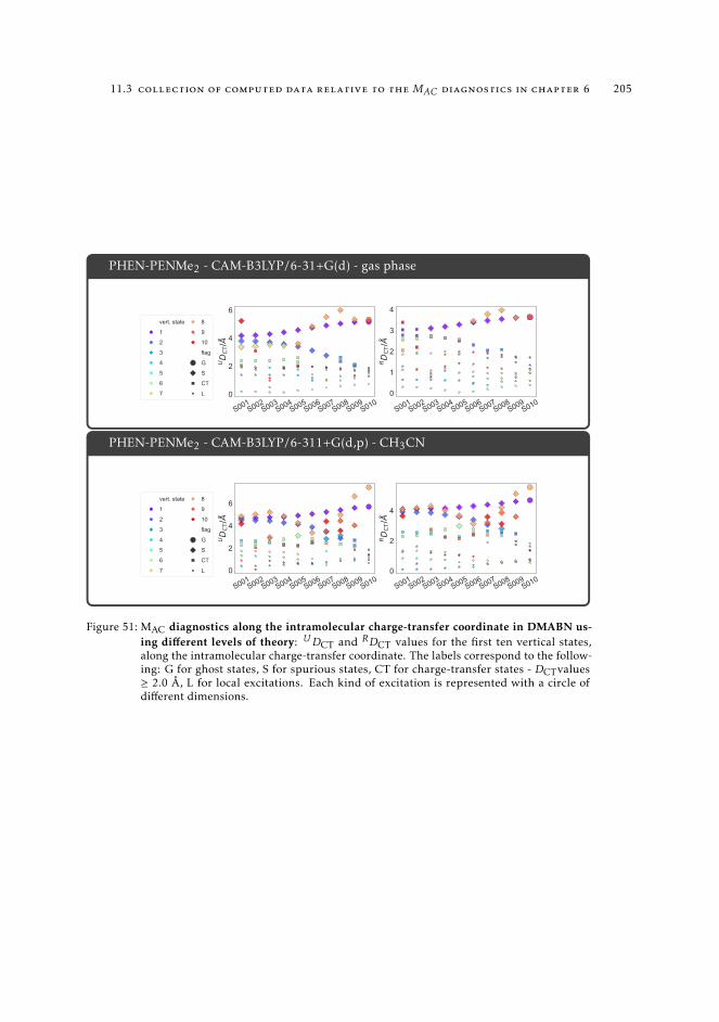
11.3 collection of computed data relative to the MAC diagnostics in chapter 6 205
PHEN-PENMe2 - CAM-B3LYP/6-31+G(d) - gas phase
S001S002
S003S004
S005S006
S007S008
S009S010
0
2
4
6
UD
CT/Å
vert. state
1
2
3
4
5
6
7
8
9
10
flag
G
S
CT
L
S001S002
S003S004
S005S006
S007S008
S009S010
0
1
2
3
4
RD
CT/Å
PHEN-PENMe2 - CAM-B3LYP/6-311+G(d,p) - CH3CN
S001S002
S003S004
S005S006
S007S008
S009S010
0
2
4
6
UD
CT/Å
vert. state
1
2
3
4
5
6
7
8
9
10
flag
G
S
CT
L
S001S002
S003S004
S005S006
S007S008
S009S010
0
2
4
RD
CT/Å
Figure 51: MAC diagnostics along the intramolecular charge-transfer coordinate in DMABN us-ing different levels of theory: UDCT and RDCT values for the first ten vertical states,along the intramolecular charge-transfer coordinate. The labels correspond to the follow-ing: G for ghost states, S for spurious states, CT for charge-transfer states - DCTvalues≥ 2.0 Å, L for local excitations. Each kind of excitation is represented with a circle ofdifferent dimensions.
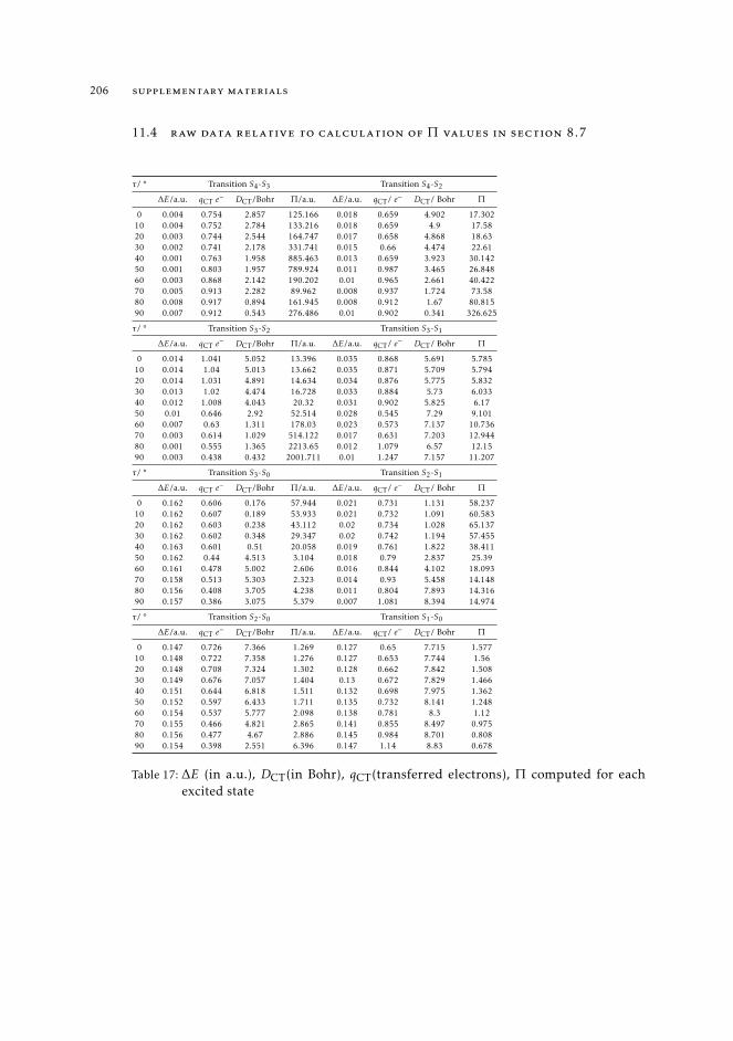
206 supplementary materials
11.4 raw data relative to calculation of Π values in section 8.7
τ/ ° Transition S4-S3 Transition S4-S2
∆E/a.u. qCT e− DCT/Bohr Π/a.u. ∆E/a.u. qCT/ e− DCT/ Bohr Π
0 0.004 0.754 2.857 125.166 0.018 0.659 4.902 17.30210 0.004 0.752 2.784 133.216 0.018 0.659 4.9 17.5820 0.003 0.744 2.544 164.747 0.017 0.658 4.868 18.6330 0.002 0.741 2.178 331.741 0.015 0.66 4.474 22.6140 0.001 0.763 1.958 885.463 0.013 0.659 3.923 30.14250 0.001 0.803 1.957 789.924 0.011 0.987 3.465 26.84860 0.003 0.868 2.142 190.202 0.01 0.965 2.661 40.42270 0.005 0.913 2.282 89.962 0.008 0.937 1.724 73.5880 0.008 0.917 0.894 161.945 0.008 0.912 1.67 80.81590 0.007 0.912 0.543 276.486 0.01 0.902 0.341 326.625
τ/ ° Transition S3-S2 Transition S3-S1
∆E/a.u. qCT e− DCT/Bohr Π/a.u. ∆E/a.u. qCT/ e− DCT/ Bohr Π
0 0.014 1.041 5.052 13.396 0.035 0.868 5.691 5.78510 0.014 1.04 5.013 13.662 0.035 0.871 5.709 5.79420 0.014 1.031 4.891 14.634 0.034 0.876 5.775 5.83230 0.013 1.02 4.474 16.728 0.033 0.884 5.73 6.03340 0.012 1.008 4.043 20.32 0.031 0.902 5.825 6.1750 0.01 0.646 2.92 52.514 0.028 0.545 7.29 9.10160 0.007 0.63 1.311 178.03 0.023 0.573 7.137 10.73670 0.003 0.614 1.029 514.122 0.017 0.631 7.203 12.94480 0.001 0.555 1.365 2213.65 0.012 1.079 6.57 12.1590 0.003 0.438 0.432 2001.711 0.01 1.247 7.157 11.207
τ/ ° Transition S3-S0 Transition S2-S1
∆E/a.u. qCT e− DCT/Bohr Π/a.u. ∆E/a.u. qCT/ e− DCT/ Bohr Π
0 0.162 0.606 0.176 57.944 0.021 0.731 1.131 58.23710 0.162 0.607 0.189 53.933 0.021 0.732 1.091 60.58320 0.162 0.603 0.238 43.112 0.02 0.734 1.028 65.13730 0.162 0.602 0.348 29.347 0.02 0.742 1.194 57.45540 0.163 0.601 0.51 20.058 0.019 0.761 1.822 38.41150 0.162 0.44 4.513 3.104 0.018 0.79 2.837 25.3960 0.161 0.478 5.002 2.606 0.016 0.844 4.102 18.09370 0.158 0.513 5.303 2.323 0.014 0.93 5.458 14.14880 0.156 0.408 3.705 4.238 0.011 0.804 7.893 14.31690 0.157 0.386 3.075 5.379 0.007 1.081 8.394 14.974
τ/ ° Transition S2-S0 Transition S1-S0
∆E/a.u. qCT e− DCT/Bohr Π/a.u. ∆E/a.u. qCT/ e− DCT/ Bohr Π
0 0.147 0.726 7.366 1.269 0.127 0.65 7.715 1.57710 0.148 0.722 7.358 1.276 0.127 0.653 7.744 1.5620 0.148 0.708 7.324 1.302 0.128 0.662 7.842 1.50830 0.149 0.676 7.057 1.404 0.13 0.672 7.829 1.46640 0.151 0.644 6.818 1.511 0.132 0.698 7.975 1.36250 0.152 0.597 6.433 1.711 0.135 0.732 8.141 1.24860 0.154 0.537 5.777 2.098 0.138 0.781 8.3 1.1270 0.155 0.466 4.821 2.865 0.141 0.855 8.497 0.97580 0.156 0.477 4.67 2.886 0.145 0.984 8.701 0.80890 0.154 0.398 2.551 6.396 0.147 1.14 8.83 0.678
Table 17: ∆E (in a.u.), DCT(in Bohr), qCT(transferred electrons), Π computed for eachexcited state
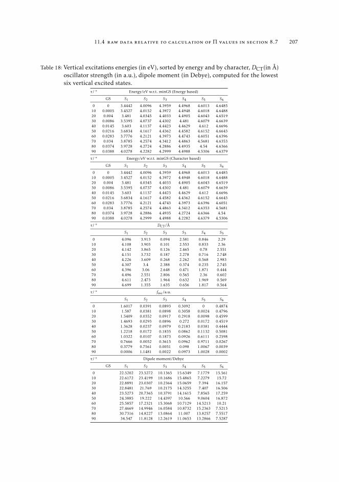
11.4 raw data relative to calculation of Π values in section 8.7 207
Table 18: Vertical excitations energies (in eV), sorted by energy and by character, DCT(in Å)oscillator strength (in a.u.), dipole moment (in Debye), computed for the lowestsix vertical excited states.
τ/ ° Energy/eV w.r.t. minGS (Energy based)
GS S1 S2 S3 S4 S5 S6
0 0 3.4442 4.0096 4.3959 4.4968 4.6013 4.648510 0.0005 3.4527 4.0152 4.3972 4.4948 4.6018 4.648820 0.004 3.481 4.0345 4.4033 4.4905 4.6043 4.651930 0.0086 3.5395 4.0737 4.4302 4.481 4.6079 4.663940 0.0145 3.603 4.1137 4.4423 4.4629 4.612 4.669650 0.0216 3.6834 4.1617 4.4362 4.4582 4.6152 4.664360 0.0283 3.7776 4.2121 4.3973 4.4743 4.6051 4.639670 0.034 3.8785 4.2574 4.3412 4.4863 4.5681 4.635380 0.0374 3.9728 4.2724 4.2886 4.4935 4.54 4.636690 0.0388 4.0278 4.2282 4.2999 4.4988 4.5306 4.6379
τ/ ° Energy/eV w.r.t. minGS (Character based)
GS S1 S2 S3 S4 S5 S6
0 0 3.4442 4.0096 4.3959 4.4968 4.6013 4.648510 0.0005 3.4527 4.0152 4.3972 4.4948 4.6018 4.648820 0.004 3.481 4.0345 4.4033 4.4905 4.6043 4.651930 0.0086 3.5395 4.0737 4.4302 4.481 4.6079 4.663940 0.0145 3.603 4.1137 4.4423 4.4629 4.612 4.669650 0.0216 3.6834 4.1617 4.4582 4.4362 4.6152 4.664360 0.0283 3.7776 4.2121 4.4743 4.3973 4.6396 4.605170 0.034 3.8785 4.2574 4.4863 4.3412 4.6353 4.568180 0.0374 3.9728 4.2886 4.4935 4.2724 4.6366 4.5490 0.0388 4.0278 4.2999 4.4988 4.2282 4.6379 4.5306
τ/ ° DCT/Å
S1 S2 S3 S3 S4 S5
0 4.096 3.913 0.094 2.581 0.846 2.2910 4.108 3.903 0.101 2.553 0.833 2.3620 4.142 3.865 0.126 2.465 0.78 2.55130 4.151 3.732 0.187 2.278 0.716 2.74840 4.226 3.609 0.268 2.262 0.568 2.98350 4.307 3.4 2.388 0.374 0.235 2.74560 4.396 3.06 2.648 0.471 1.871 0.44470 4.496 2.551 2.806 0.565 2.36 0.60280 4.611 2.473 1.964 0.632 1.969 0.56990 4.699 1.355 1.635 0.656 1.817 0.564
τ/ ° fosc/a.u.
S1 S2 S3 S4 S5 S6
0 1.6017 0.0391 0.0893 0.3092 0 0.487410 1.587 0.0381 0.0898 0.3058 0.0024 0.479620 1.5409 0.0352 0.0917 0.2918 0.0098 0.459930 1.4693 0.0293 0.0896 0.272 0.0172 0.451940 1.3628 0.0237 0.0979 0.2183 0.0381 0.444450 1.2218 0.0172 0.1835 0.0862 0.1132 0.508160 1.0322 0.0107 0.1873 0.0926 0.6111 0.259870 0.7666 0.0052 0.3615 0.0962 0.9711 0.026780 0.3779 0.7561 0.0051 0.098 1.0067 0.003990 0.0006 1.1481 0.0022 0.0973 1.0028 0.0002
τ/ ° Dipole moment/Debye
GS S1 S2 S3 S4 S5 S6
0 22.5202 23.5272 10.1365 15.6349 7.1779 15.56110 22.6172 23.4199 10.1686 15.4865 7.2279 15.7220 22.8891 23.0307 10.2364 15.0659 7.394 16.15730 22.8481 21.769 10.2175 14.3255 7.407 16.50640 23.5273 20.7365 10.3791 14.1615 7.8565 17.25950 24.3885 19.222 14.4397 10.566 9.0604 16.87260 25.5857 17.2321 15.3068 10.7129 14.5213 10.2170 27.4669 14.9946 16.0584 10.8732 15.2363 7.521380 30.7316 14.8227 13.0864 11.007 13.8257 7.551790 34.547 11.8128 12.2619 11.0653 13.2866 7.5287
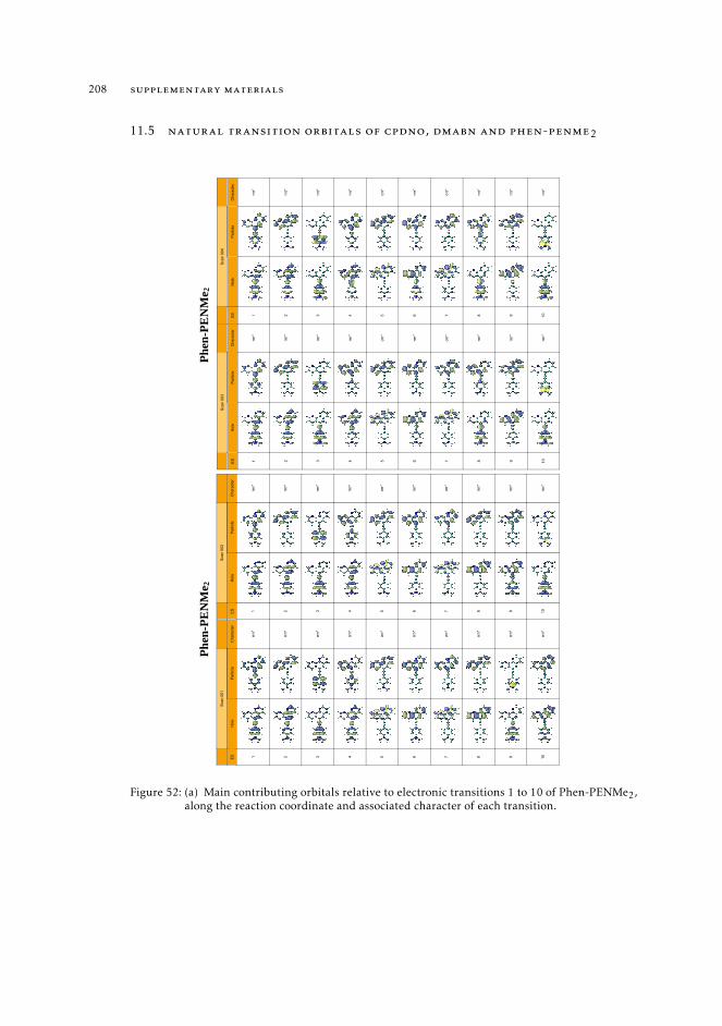
208 supplementary materials
11.5 natural transition orbitals of cpdno, dmabn and phen-penme2
Phen
-PE
NM
e 2Ph
en-P
EN
Me 2
Scan0
01Sc
an0
02
ESH
ole
Parti
cle
Cha
ract
erES
Hol
ePa
rticl
eC
hara
cter
1π
π*
1π
π*
2π
π*
2π
π*
3π
π*
3π
π*
4π
π*
4π
π*
5σπ
*5
σπ*
6π
π*
6π
π*
7σπ
*7
σπ*
8π
π*
8π
π*
9π
π*
9π
π*
10π
π*
10π
π*
Scan0
03Sc
an0
04
ESH
ole
Parti
cle
Cha
ract
erES
Hol
ePa
rticl
eC
hara
cter
1π
π*
1π
π*
2π
π*
2π
π*
3π
π*
3π
π*
4π
π*
4π
π*
5σπ
*5
σπ*
6π
π*
6π
π*
7σπ
*7
σπ*
8π
π*
8π
π*
9π
π*
9π
π*
10π
π*
10π
π*
Figure 52: (a) Main contributing orbitals relative to electronic transitions 1 to 10 of Phen-PENMe2,along the reaction coordinate and associated character of each transition.
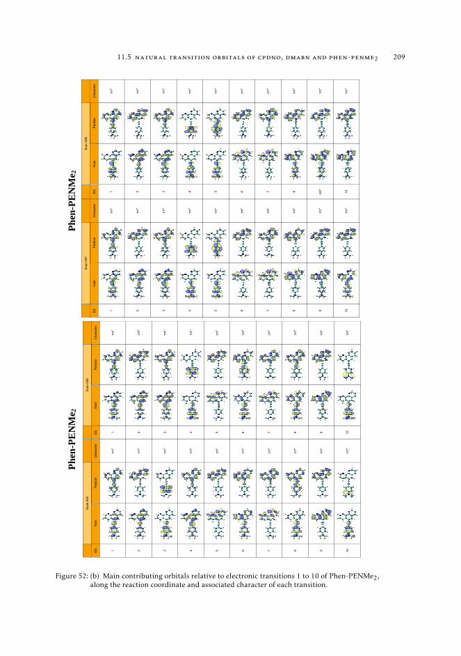
11.5 natural transition orbitals of cpdno, dmabn and phen-penme2 209
Phen
-PE
NM
e 2Ph
en-P
EN
Me 2
Scan0
05Sc
an0
06
ESH
ole
Parti
cle
Cha
ract
erES
Hol
ePa
rticl
eC
hara
cter
1π
π*
1π
π*
2π
π*
2π
π*
3π
π*
3π
π*
4π
π*
4π
π*
5σπ
*5
σπ*
6π
π*
6π
π*
7σπ
*7
σπ*
8π
π*
8π
π*
9π
π*
9π
π*
10π
π*
10π
π*
Scan0
07Sc
an0
08
ESH
ole
Parti
cle
Cha
ract
erES
Hol
ePa
rticl
eC
hara
cter
1π
π*
1π
π*
2π
π*
2π
π*
3π
π*
3π
π*
4π
π*
4π
π*
5π
π*
5π
π*
6σπ
*6
σπ*
7σπ
*7
σπ*
8π
π*
8π
π*
9π
π*
ππ
*π
π*
10π
π*
10π
π*
Figure 52: (b) Main contributing orbitals relative to electronic transitions 1 to 10 of Phen-PENMe2,along the reaction coordinate and associated character of each transition.
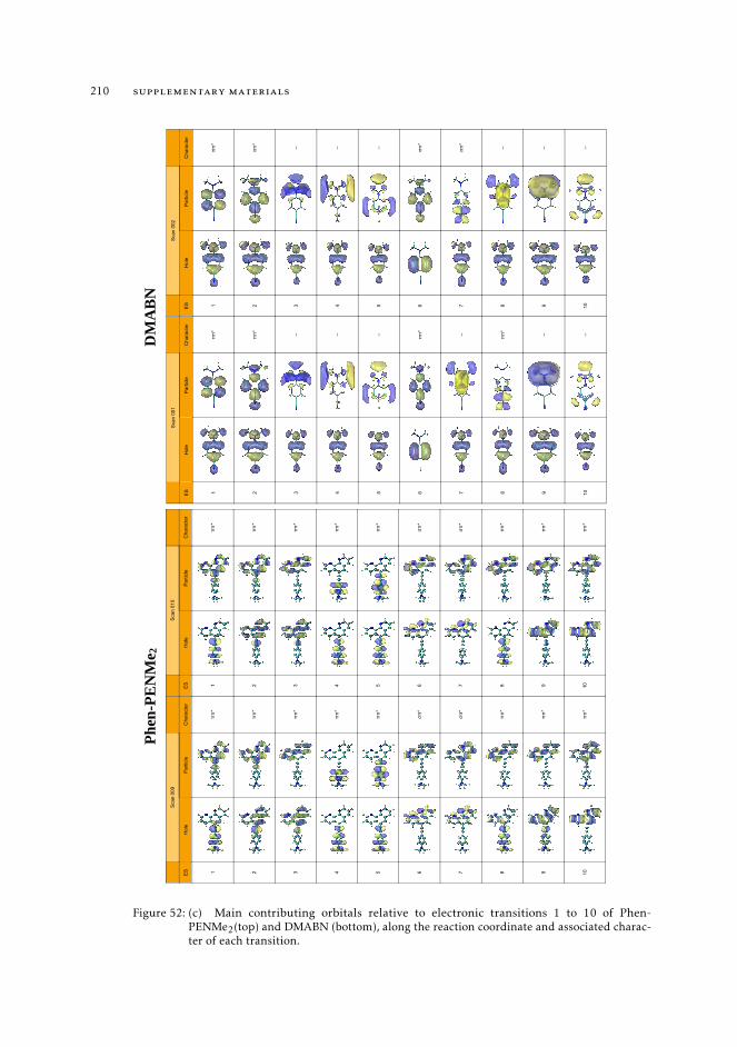
210 supplementary materials
Phen
-PE
NM
e 2D
MA
BN
Scan0
09Sc
an0
10
ESH
ole
Parti
cle
Cha
ract
erES
Hol
ePa
rticl
eC
hara
cter
1π
π*
1π
π*
2π
π*
2π
π*
3π
π*
3π
π*
4π
π*
4π
π*
5π
π*
5π
π*
6σπ
*6
σπ*
7σπ
*7
σπ*
8π
π*
8π
π*
9π
π*
9π
π*
10π
π*
10π
π*
Scan0
01Sc
an0
02
ESH
ole
Parti
cle
Cha
ract
erES
Hol
ePa
rticl
eC
hara
cter
1π
π*
1π
π*
2π
π*
2π
π*
3--
3--
4--
4--
5--
5--
6π
π*
6π
π*
7--
7π
π*
8π
π*
8--
9--
9--
10--
10--
Figure 52: (c) Main contributing orbitals relative to electronic transitions 1 to 10 of Phen-PENMe2(top) and DMABN (bottom), along the reaction coordinate and associated charac-ter of each transition.
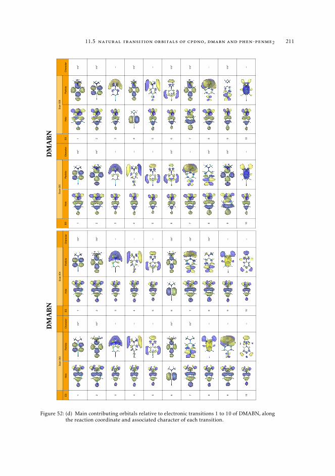
11.5 natural transition orbitals of cpdno, dmabn and phen-penme2 211D
MA
BN
DM
AB
NSc
an0
03Sc
an0
04
ESH
ole
Parti
cle
Cha
ract
erES
Hol
ePa
rticl
eC
hara
cter
1π
π*
1π
π*
2π
π*
2π
π*
3--
3--
4--
4--
5--
5--
6π
π*
6π
π*
7π
π*
7π
π*
8--
8π
π*
9--
9--
10--
10--
Scan0
05Sc
an0
06
ESH
ole
Parti
cle
Cha
ract
erES
Hol
ePa
rticl
eC
hara
cter
1π
π*
1π
π*
2π
π*
2π
π*
3--
3--
4--
4π
π*
5--
5--
6π
π*
6π
π*
7--
7π
π*
8π
π*
8-
9π
π*
9π
π*
10--
10--
Figure 52: (d) Main contributing orbitals relative to electronic transitions 1 to 10 of DMABN, alongthe reaction coordinate and associated character of each transition.
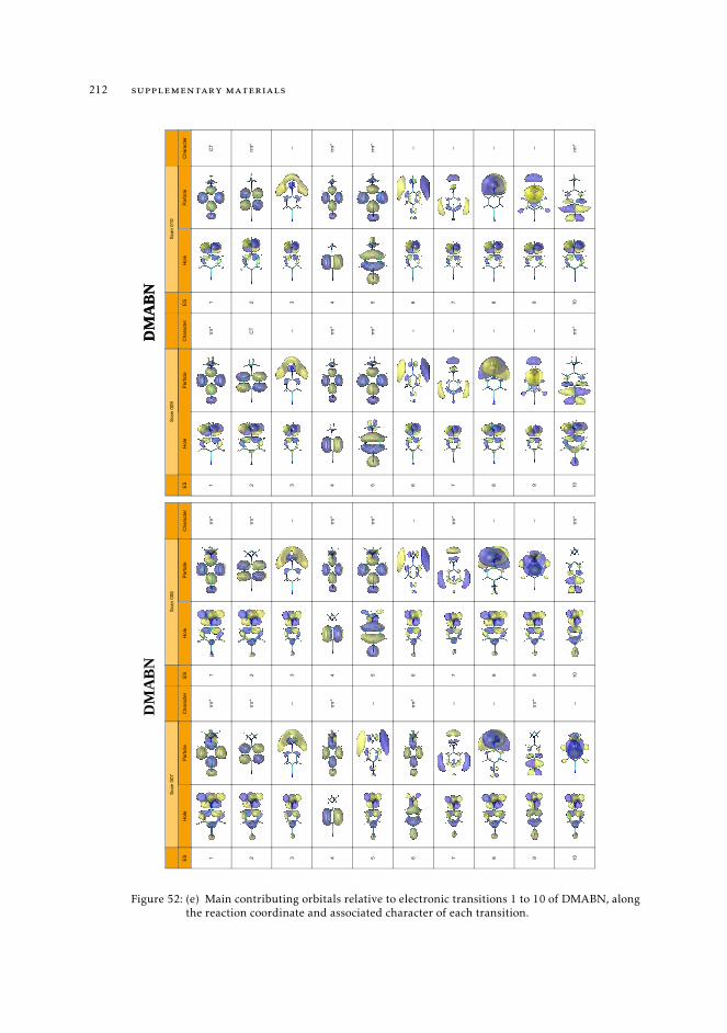
212 supplementary materials
DM
AB
ND
MA
BN
DM
AB
NSc
an0
07Sc
an0
08
ESH
ole
Parti
cle
Cha
ract
erES
Hol
ePa
rticl
eC
hara
cter
1π
π*
1π
π*
2π
π*
2π
π*
3--
3--
4π
π*
4π
π*
5--
5π
π*
6π
π*
6--
7--
7π
π*
8--
8--
9π
π*
9--
10--
10π
π*
Scan0
09Sc
an0
10
ESH
ole
Parti
cle
Cha
ract
erES
Hol
ePa
rticl
eC
hara
cter
1π
π*
1C
T
2C
T2
ππ
*
3--
3--
4π
π*
4π
π*
5π
π*
5π
π*
6--
6--
7--
7--
8--
8--
9--
9--
10π
π*
10nπ
*
Figure 52: (e) Main contributing orbitals relative to electronic transitions 1 to 10 of DMABN, alongthe reaction coordinate and associated character of each transition.
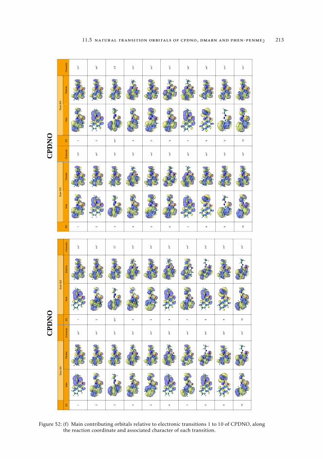
11.5 natural transition orbitals of cpdno, dmabn and phen-penme2 213
CPD
NO
CPD
NO
Scan0
01Sc
an0
02
ESH
ole
Parti
cle
Cha
ract
erES
Hol
ePa
rticl
eC
hara
cter
1σπ
*1
σπ*
2π
π*
2π
π*
3π
π*
ππ
*C
T
4π
π*
4π
π*
5π
π*
5π
π*
6σπ
*6
σπ*
7π
π*
7π
π*
8σπ
*8
σπ*
9σπ
*9
σπ*
10π
π*
10π
π*
Scan0
03Sc
an0
04
ESH
ole
Parti
cle
Cha
ract
erES
Hol
ePa
rticl
eC
hara
cter
1π
π*
1π
π*
2σπ
*2
σπ*
3π
π*
ππ
*C
T
4π
π*
4π
π*
5π
π*
5π
π*
6π
π*
6π
π*
7σπ
*7
σπ*
8σπ
*8
σπ*
9π
π*
9π
π*
10π
π*
10π
π*
Figure 52: (f) Main contributing orbitals relative to electronic transitions 1 to 10 of CPDNO, alongthe reaction coordinate and associated character of each transition.
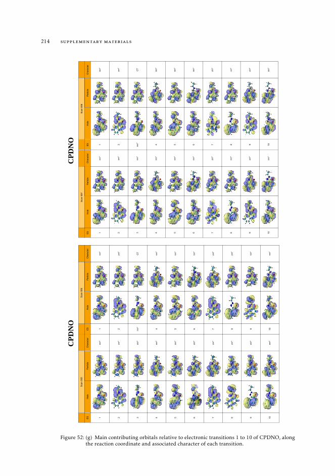
214 supplementary materials
CPD
NO
CPD
NO
Scan0
05Sc
an0
06
ESH
ole
Parti
cle
Cha
ract
erES
Hol
ePa
rticl
eC
hara
cter
1π
π*
1π
π*
2σπ
*2
σπ*
3π
π*
ππ
*C
T
4π
π*
4π
π*
5π
π*
5π
π*
6π
π*
6π
π*
7σπ
*7
σπ*
8σπ
*8
σπ*
9π
π*
9π
π*
10π
π*
10π
π*
Scan0
07Sc
an0
08
ESH
ole
Parti
cle
Cha
ract
erES
Hol
ePa
rticl
eC
hara
cter
1π
π*
1π
π*
2σπ
*2
σπ*
3π
π*
ππ
*C
T
4π
π*
4π
π*
5π
π*
5π
π*
6π
π*
6π
π*
7σπ
*7
σπ*
8π
π*
8nπ
*
9σπ
*9
σπ*
10π
π*
10π
π*
Figure 52: (g) Main contributing orbitals relative to electronic transitions 1 to 10 of CPDNO, alongthe reaction coordinate and associated character of each transition.
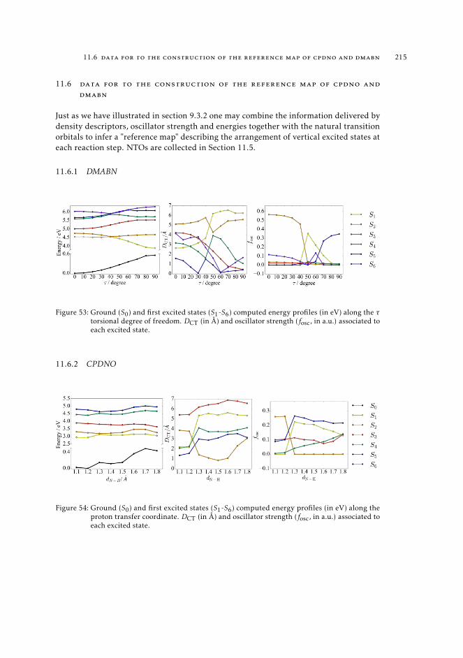
11.6 data for to the construction of the reference map of cpdno and dmabn 215
11.6 data for to the construction of the reference map of cpdno and
dmabn
Just as we have illustrated in section 9.3.2 one may combine the information delivered bydensity descriptors, oscillator strength and energies together with the natural transitionorbitals to infer a "reference map" describing the arrangement of vertical excited states ateach reaction step. NTOs are collected in Section 11.5.
11.6.1 DMABN
Figure 53: Ground (S0) and first excited states (S1-S6) computed energy profiles (in eV) along the τtorsional degree of freedom. DCT (in Å) and oscillator strength (fosc, in a.u.) associated toeach excited state.
11.6.2 CPDNO
Figure 54: Ground (S0) and first excited states (S1-S6) computed energy profiles (in eV) along theproton transfer coordinate. DCT (in Å) and oscillator strength (fosc, in a.u.) associated toeach excited state.
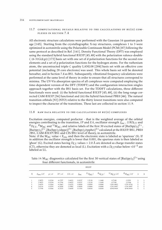
216 supplementary materials
11.7 computational details relative to the calculations of ru(ii) com-
plexes in section 7.4
All electronic structure calculations were performed with the Gaussian 16 quantum pack-age [145]. Starting from the crystallographic X-ray structures, complexes 1 to 3 wereoptimized in acetonitrile using the Polarizable Continuum Model (PCM) [87] following thesame protocol as described in Ref. [161]. Density Functional Theory (DFT) was employedusing the standard hybrid functional B3LYP [45, 48] with the polarization valence-double-ζ (6-31G(d,p)) [172] basis set with one set of d polarization functions for the second-rowelements and a set of p polarization functions for the hydrogen atoms. For the rutheniumatom, the uncontracted triple-ζ quality LANL08 [284] basis set with an effective corepotential (including 28 core electrons) was used. This whole basis set will be denotedhereafter, and in Section 7.4 as BS1. Subsequently, vibrational frequency calculations wereperformed at the same level of theory in order to ensure that all structures correspond tominima. The UV-Vis absorption spectra of all complexes were computed employing thetime-dependent version of the DFT (TDDFT) and the configuration interaction singlesapproach together with the BS1 basis set. For the TDDFT calculations, three differentfunctionals were used: (i) the hybrid functional B3LYP [45, 48], (ii) the long-range cor-rected CAM-B3LYP [56] functional and (iii) the hybrid functional PBE0 [46]. The naturaltransition orbitals [92] (NTO) relative to the thirty lowest transitions were also computedto inspect the character of the transitions. These last are collected in section 11.9.
11.8 raw data relative to the calculations of ru(ii) complexes
Excitation energies, computed prefactor - that is the weighted average of the orbitalenergies contributing to the transition, IP and EA, oscillator strength fosc , URDCT andRDCT, RMAC and UMAC, and relative labels of the first 30 excited states of [Ru(bpy)3]2+,[Ru(tpy)2]2+,[Ru(bpy)2(dppz)]2+,[Ru(bpy)2(tpphz)]2+calculated at the B3LYP/BS1, PBE0/BS1, CAM-B3LYP/BS1 and CIS/BS1 level of theory, in acetonitrile.Note: if the MAC value < Eexc and then the electronic state is labeled as ’spurious’ (S). Ifin addition the oscillator strength is lower that 0.001, the spurious state is then labeled as’ghost’ (G). Excited states having DCT values > 2.0 Å are denoted as charge-transfer states(CT), otherwise they are demoted as local (L). Excitation with a DCTvalue below ∗10−5 arelabeled as LL.
Table 19: MAC diagnostics calculated for the first 30 vertical states of [Ru(tpy)2]2+usingfour different functionals, in acetonitrile
B3LYP
N Eexc/eV p / eV IP / eV EA / eV fosc UDDC/ RDCT/ UMCT/eV RMAC/eV U R
1 2.5875 0.3234 -6.1797 -2.6022 0.0237 1.5130 1.1680 -0.7180 -3.5291 L L2 2.5875 0.3234 -6.1796 -2.6022 0.0237 1.5130 1.1690 -0.7180 -3.5186 L L3 2.6070 0.3264 -6.2463 -2.6225 0.0000 0.0090 0.0080 -1591.0802 -1791.0754 L L4 2.6710 0.3255 -6.2458 -2.5982 0.0000 0.0080 0.0080 -1791.0997 -1791.0997 L L5 2.7790 0.3266 -6.2525 -2.6050 0.1783 0.0030 0.0030 -4790.9959 -4790.9959 L L

11.8 raw data relative to the calculations of ru(ii) complexes 217
6 2.8650 0.3212 -6.2200 -2.4962 0.0000 0.0030 0.0030 -4791.1448 -4791.1448 L L7 2.9565 0.3193 -6.1830 -2.4916 0.1742 0.0020 0.0010 -7191.1374 -14390.9632 L L8 2.9752 0.3209 -6.2527 -2.4669 0.0686 1.5880 1.2480 -0.3364 -2.8068 L L9 2.9754 0.3209 -6.2529 -2.4670 0.0685 1.5840 1.2460 -0.3590 -2.8250 L L10 2.9925 0.3184 -6.2450 -2.4126 0.0086 2.6310 1.6900 3.1916 0.1441 S L11 2.9926 0.3184 -6.2452 -2.4125 0.0087 2.6280 1.6880 3.1855 0.1342 S L12 3.2728 0.3158 -6.2824 -2.2367 0.0000 0.0020 0.0020 -7191.2336 -7191.2336 L L13 3.2795 0.2621 -6.2383 -0.8277 0.0000 0.0010 0.0010 -14392.5188 -14392.5188 L L14 3.6763 0.2582 -6.2922 -0.6501 0.0011 0.7350 0.5160 -12.5655 -20.8805 L L15 3.6768 0.2582 -6.2925 -0.6501 0.0011 0.7350 0.5160 -12.5653 -20.8802 L L16 3.8486 0.2870 -6.2008 -1.5894 0.0506 0.0050 0.0040 -2872.1196 -3592.1022 L L17 3.8671 0.3289 -6.8063 -2.1184 0.0825 0.3470 0.3900 -32.5469 -27.9716 L L18 3.8672 0.3289 -6.8063 -2.1184 0.0824 0.3480 0.3910 -32.4278 -27.8772 L L19 3.8787 0.2881 -6.2512 -1.5777 0.0038 0.7060 0.4180 -12.5570 -26.6098 L L20 3.8789 0.2881 -6.2514 -1.5777 0.0038 0.7060 0.4180 -12.5569 -26.6098 L L21 3.9625 0.2843 -6.2450 -1.4836 0.0000 1.6030 1.0810 -1.2465 -5.5842 L L22 3.9627 0.2843 -6.2452 -1.4836 0.0000 1.6030 1.0810 -1.2462 -5.5839 L L23 3.9917 0.2863 -6.2723 -1.5021 0.0002 0.0670 0.0880 -207.1303 -155.8426 L L24 3.9937 0.2859 -6.2661 -1.4978 0.0262 0.0670 0.0870 -207.1416 -157.7347 L L25 4.0055 0.3202 -6.6894 -1.9841 0.6349 1.3120 1.1290 -2.2609 -4.0399 L L26 4.0055 0.3203 -6.6896 -1.9844 0.6345 1.3140 1.1310 -2.2437 -4.0169 L L27 4.0529 0.2810 -6.3767 -1.2331 0.0065 0.3560 0.4020 -32.8032 -28.1748 L L28 4.0531 0.2812 -6.3796 -1.2373 0.0069 0.3740 0.4160 -30.8495 -26.9623 L L29 4.0671 0.3489 -7.0807 -2.4006 0.1355 3.1210 2.2290 4.8794 3.0331 S CT30 4.0671 0.3491 -7.0831 -2.4039 0.1357 3.1320 2.2310 4.9013 3.0445 S CT
CAM-B3LYP
N Eexc/eV p / eV IP / eV EA / eV fosc UDDC/ RDCT/ UMCT/eV RMAC/eV U R
1 3.1055 0.3328 -7.5850 -1.2990 0.0241 1.8670 1.3690 1.3426 -1.4630 L L2 3.1056 0.3328 -7.5850 -1.2990 0.0241 1.8680 1.3690 1.3467 -1.4630 L L3 3.1827 0.3314 -7.6983 -0.3082 0.0000 0.0050 0.0050 -2870.9120 -2870.9120 L L4 3.2408 0.3296 -7.7017 0.0207 0.0000 0.0020 0.0020 -7190.8572 -7190.8572 L L5 3.2454 0.3371 -7.6819 -1.3786 0.2541 0.0020 0.0020 -7190.6539 -7190.6539 L L6 3.2548 0.3372 -7.6895 -1.3288 0.0001 0.0050 0.0050 -2870.7536 -2870.7536 L L7 3.4468 0.3342 -7.6835 -1.2718 0.0000 0.0030 0.0040 -4790.7902 -3590.8192 L L8 3.6457 0.3296 -7.7557 0.5157 0.0352 0.8300 0.7520 -8.3790 -10.1785 L L9 3.6459 0.3296 -7.7553 0.5032 0.0358 0.8380 0.7610 -8.2140 -9.9526 L L10 3.6995 0.3305 -7.7047 -0.5775 0.0742 1.8310 1.5250 1.1298 -0.4483 L L11 3.6996 0.3305 -7.7044 -0.5901 0.0749 1.8350 1.5270 1.1462 -0.4366 L L12 3.7647 0.3261 -7.5714 -1.2499 0.1874 0.0020 0.0020 -7190.9515 -7190.9515 L L13 3.8588 0.3299 -7.6893 -1.0349 0.0039 2.1600 1.4950 2.3096 -0.6558 CT L14 3.8590 0.3299 -7.6896 -1.0349 0.0039 2.1600 1.4950 2.3098 -0.6555 CT L15 3.9786 0.3294 -7.6680 -1.1481 0.0000 0.0010 0.0010 -14390.6874 -14390.6874 L L16 4.2372 0.3452 -7.8360 1.2134 0.0373 0.1020 0.0700 -131.7789 -196.3151 L L17 4.2375 0.3452 -7.8361 1.2127 0.0375 0.1020 0.0700 -131.7787 -196.3149 L L18 4.3252 0.3699 -8.6143 -1.0706 0.6287 0.3370 0.3900 -32.6643 -26.8576 L L19 4.3253 0.3699 -8.6140 -1.0698 0.6285 0.3360 0.3890 -32.7917 -26.9527 L L20 4.6202 0.3451 -7.6676 1.6572 0.0002 0.0000 0.0000 -2721130.2216 -2721130.2216 LL LL21 4.6740 0.3321 -8.2387 -0.6507 0.5156 0.0070 0.0060 -2048.0562 -2390.9050 L L22 4.7464 0.3689 -8.7406 -1.0665 0.0000 0.0020 0.0020 -7189.7869 -7189.7869 L L23 4.8299 0.2907 -7.6688 -0.1414 0.3550 0.6890 0.6910 -12.9885 -12.9280 L L24 4.8301 0.2907 -7.6691 -0.1417 0.3553 0.6940 0.6930 -12.8374 -12.8673 L L25 4.8364 0.3290 -8.1343 -0.6356 0.4071 0.1380 0.1160 -95.3918 -115.1815 L L26 4.8846 0.2935 -7.6996 -0.2029 0.0871 0.4650 0.2050 -22.9818 -62.2570 L L27 4.8848 0.2935 -7.6998 -0.2029 0.0866 0.4660 0.2060 -22.9150 -61.9157 L L28 4.9423 0.2904 -7.7109 -0.1148 0.0000 0.2200 0.1750 -57.5497 -74.3804 L L29 4.9435 0.2904 -7.7086 -0.1130 0.0001 0.2200 0.1740 -57.5518 -74.8555 L L30 4.9733 0.2942 -7.7482 -0.1473 0.0012 0.0770 0.1100 -179.0036 -122.9010 L L
CIS
N Eexc/eV p / eV IP / eV EA / eV fosc UDDC/ RDCT/ UMCT/eV RMAC/eV U R
1 2.7282 0.6037 -10.1492 6.2776 0.0000 0.0000 0.0000 -2721123.1863 -2721123.1863 LL LL2 3.3099 0.6180 -10.2286 6.5869 0.0008 0.3370 0.3860 -25.9134 -20.4893 L L3 3.3104 0.6180 -10.2288 6.5874 0.0008 0.3370 0.3860 -25.9127 -20.4885 L L4 4.4280 0.6094 -10.1697 6.4131 0.0000 0.1220 0.0390 -101.4472 -352.6391 L L5 4.4284 0.6094 -10.1694 6.4135 0.0000 0.1220 0.0390 -101.4470 -352.6389 L L6 4.7612 0.3907 -9.3746 1.2560 0.6526 0.1740 0.2450 -72.1260 -48.1435 L L
218 supplementary materials
7 4.7614 0.3907 -9.3746 1.2560 0.6527 0.1740 0.2450 -72.1260 -48.1434 L L8 4.8408 0.6104 -10.0794 6.5298 0.0001 0.0010 0.0010 -14383.0425 -14383.0425 L L9 4.9444 0.4063 -9.5937 1.4621 0.3703 0.0080 0.0080 -1788.9006 -1788.9006 L L10 4.9684 0.4073 -9.5714 1.5107 0.0000 0.0080 0.0080 -1788.8744 -1788.8744 L L11 5.5829 0.4101 -9.7841 1.3764 0.3971 1.7440 1.2270 2.9037 -0.5752 L L12 5.5830 0.4101 -9.7841 1.3765 0.3969 1.7440 1.2280 2.9040 -0.5654 L L13 5.6271 0.4069 -9.6986 1.3725 1.4847 0.0080 0.0070 -1788.8854 -2046.0220 L L14 5.7144 0.4056 -9.9332 1.1037 0.0000 0.0040 0.0030 -3588.8760 -4788.8470 L L15 5.8182 0.4148 -9.9078 1.3796 0.0001 0.0040 0.0030 -3588.6256 -4788.5966 L L16 5.8605 0.4249 -9.9811 1.5802 0.0519 1.6430 1.3500 2.7971 0.8949 L L17 5.8608 0.4249 -9.9815 1.5804 0.0519 1.6430 1.3500 2.7976 0.8955 L L18 5.9265 0.4476 -10.1138 2.0661 0.0000 0.0010 0.0000 -14387.4718 -2721127.4333 L LL19 5.9364 0.4445 -10.1718 1.9225 0.4987 0.0020 0.0020 -7187.7316 -7187.7316 L L20 6.0305 0.4096 -9.7934 1.3522 0.0000 0.0030 0.0030 -4788.7382 -4788.7382 L L21 6.3721 0.4542 -10.0694 2.2901 0.5373 0.9230 0.7510 -3.2415 -6.8146 L L22 6.3721 0.4542 -10.0694 2.2901 0.5372 0.9240 0.7520 -3.2246 -6.7890 L L23 6.5383 0.4376 -10.3079 1.5996 0.1230 2.1570 1.3710 5.2317 1.4044 CT L24 6.5386 0.4376 -10.3082 1.5994 0.1229 2.1570 1.3710 5.2318 1.4045 CT L25 6.6471 0.4586 -10.4257 2.0546 0.0035 0.0120 0.0100 -1187.4906 -1427.4848 L L26 6.6622 0.4591 -10.5133 1.9801 0.0000 0.0130 0.0110 -1095.1721 -1296.5658 L L27 6.8053 0.4562 -10.3997 2.0134 0.6558 1.0720 0.9860 -1.0194 -2.1910 L L28 6.8055 0.4562 -10.3998 2.0133 0.6561 1.0720 0.9850 -1.0195 -2.2059 L L29 6.8544 0.4391 -9.9321 2.0167 0.9776 0.0060 0.0040 -2387.9932 -3587.9641 L L30 6.9191 0.4382 -9.9966 1.9275 0.0000 0.0010 0.0010 -14387.7277 -14387.7277 L L
PBE0
N Eexc/eV p / eV IP / eV EA / eV fosc UDDC/ RDCT/ UMCT/eV RMAC/eV U R
1 2.6956 0.3329 -6.4891 -2.5456 0.0243 1.6390 1.2510 0.2729 -2.4519 L L2 2.6957 0.3329 -6.4891 -2.5455 0.0243 1.6400 1.2510 0.2783 -2.4520 L L3 2.7286 0.3365 -6.5714 -2.5657 0.0000 0.0070 0.0070 -2047.9366 -2047.9366 L L4 2.7997 0.3356 -6.5704 -2.5437 0.0000 0.0070 0.0070 -2047.9604 -2047.9604 L L5 2.8933 0.3371 -6.5775 -2.5574 0.2100 0.0030 0.0030 -4790.7114 -4790.7114 L L6 2.9983 0.3314 -6.5414 -2.4463 0.0000 0.0030 0.0030 -4790.8658 -4790.8658 L L7 3.1141 0.3285 -6.4875 -2.4366 0.1614 0.0010 0.0010 -14390.7126 -14390.7126 L L8 3.1311 0.3295 -6.5767 -2.3724 0.0823 2.0560 1.5030 1.9625 -0.6144 CT L9 3.1313 0.3295 -6.5770 -2.3724 0.0823 2.0550 1.5030 1.9593 -0.6142 CT L10 3.1627 0.3293 -6.5673 -2.3861 0.0002 2.8700 1.8250 3.9441 1.0712 G L11 3.1629 0.3293 -6.5675 -2.3862 0.0002 2.8690 1.8250 3.9427 1.0715 G L12 3.2272 0.2658 -6.5624 -0.5746 0.0000 0.0010 0.0010 -14392.4191 -14392.4191 L L13 3.4126 0.3300 -6.5983 -2.3042 0.0000 0.0010 0.0010 -14390.6710 -14390.6710 L L14 3.6429 0.2660 -6.6287 -0.4909 0.0014 0.7240 0.5380 -12.6507 -19.5268 L L15 3.6434 0.2660 -6.6289 -0.4908 0.0014 0.7240 0.5380 -12.6506 -19.5267 L L16 4.0030 0.3585 -7.3917 -2.3195 0.2867 0.2530 0.1650 -47.1591 -77.5140 L L17 4.0031 0.3586 -7.3917 -2.3195 0.2867 0.2520 0.1650 -47.3848 -77.5139 L L18 4.0459 0.2954 -6.5190 -1.4947 0.0570 0.0010 0.0010 -14391.6127 -14391.6127 L L19 4.0971 0.2949 -6.5726 -1.4328 0.0085 0.8180 0.5050 -9.5800 -20.4907 L L20 4.0973 0.2949 -6.5728 -1.4328 0.0085 0.8170 0.5050 -9.6014 -20.4905 L L21 4.1520 0.2658 -6.5979 -0.5287 0.0637 0.4920 0.5160 -22.0359 -20.6746 L L22 4.1522 0.2658 -6.5978 -0.5300 0.0644 0.4930 0.5170 -21.9755 -20.6196 L L23 4.1835 0.2927 -6.5708 -1.3806 0.0006 1.5420 1.0390 -1.3745 -5.8954 L L24 4.1837 0.2927 -6.5716 -1.3808 0.0019 1.5410 1.0390 -1.3796 -5.8944 L L25 4.1866 0.3048 -6.7340 -1.5131 0.5090 1.2120 1.0450 -3.5867 -5.4854 L L26 4.1866 0.3048 -6.7346 -1.5121 0.5091 1.2110 1.0460 -3.5967 -5.4724 L L27 4.2111 0.2960 -6.6141 -1.4192 0.0000 0.0380 0.0520 -370.8832 -268.8614 L L28 4.2152 0.2950 -6.5998 -1.4085 0.0185 0.0420 0.0540 -334.8208 -258.6322 L L29 4.2689 0.3680 -7.4935 -2.5141 0.0586 3.6300 2.3670 6.0469 3.9303 S CT30 4.2689 0.3680 -7.4936 -2.5142 0.0585 3.6300 2.3670 6.0471 3.9305 S CT
Table 20: MAC diagnostics calculated for the first 30 vertical states of [Ru(bpy)3]2+usingfour different functionals, in acetonitrile
B3LYP
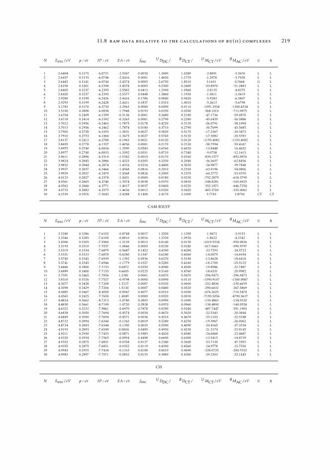
11.8 raw data relative to the calculations of ru(ii) complexes 219
N Eexc/eV p / eV IP / eV EA / eV fosc UDDC/ RDCT/ UMCT/eV RMAC/eV U R
1 2.6404 0.3175 -6.0721 -2.5567 0.0030 1.2490 1.0280 -2.8891 -5.3676 L L2 2.6437 0.3135 -6.0748 -2.4416 0.0001 1.4650 1.1770 -1.2978 -3.7028 L L3 2.6443 0.3141 -6.0744 -2.4574 0.0005 2.6750 1.8510 3.1631 0.7668 G L4 2.8238 0.3201 -6.2398 -2.4578 0.0005 0.2300 0.2400 -53.8970 -51.2883 L L5 2.8405 0.3237 -6.2395 -2.5582 0.0413 1.2390 1.0560 -2.8135 -4.8275 L L6 2.8420 0.3237 -6.2395 -2.5577 0.0448 1.3860 1.1930 -1.5811 -3.2619 L L7 2.9280 0.3199 -6.2426 -2.4416 0.1786 0.9840 0.9420 -5.9283 -6.5807 L L8 2.9293 0.3199 -6.2428 -2.4411 0.1837 1.0310 1.0010 -5.2613 -5.6798 L L9 3.1783 0.3170 -6.2730 -2.2963 0.0000 0.0090 0.0110 -1591.3354 -1300.4334 L L10 3.5100 0.2898 -6.0838 -1.7948 0.0193 0.0250 0.0200 -568.1010 -712.0975 L L11 3.6704 0.2409 -6.1599 -0.3136 0.0001 0.2680 0.2180 -47.1736 -59.4970 L L12 3.6718 0.2414 -6.1592 -0.3263 0.0001 0.2790 0.2280 -45.0439 -56.5886 L L13 3.7012 0.2956 -6.2463 -1.7875 0.0178 0.4220 0.3120 -26.0791 -38.1094 L L14 3.7013 0.2956 -6.2462 -1.7874 0.0180 0.3710 0.2790 -30.7699 -43.5685 L L15 3.7902 0.2758 -6.1055 -1.3831 0.0027 0.5820 0.5170 -17.2367 -20.3473 L L16 3.7910 0.2753 -6.1064 -1.3675 0.0027 0.5760 0.5130 -17.5082 -20.5783 L L17 3.8137 0.2412 -6.2788 -0.1965 0.0021 0.0120 0.0120 -1193.4082 -1193.4082 L L18 3.8695 0.2778 -6.1337 -1.4056 0.0001 0.2170 0.2150 -58.7994 -59.4167 L L19 3.8975 0.2740 -6.0834 -1.3590 0.0543 0.6760 0.6020 -13.8448 -16.4632 L L20 3.8977 0.2740 -6.0833 -1.3592 0.0551 0.8710 0.7340 -9.0758 -12.1615 L L21 3.9611 0.2896 -6.3314 -1.5342 0.0010 0.0170 0.0160 -839.1577 -892.0976 L L22 3.9824 0.2845 -6.2886 -1.4325 0.0205 0.3250 0.2040 -36.5657 -62.8456 L L23 3.9832 0.2844 -6.2874 -1.4316 0.0216 0.4400 0.3030 -24.9877 -39.7848 L L24 3.9927 0.2837 -6.2466 -1.4568 0.0816 0.2010 0.2330 -63.9196 -54.0806 L L25 3.9929 0.2837 -6.2470 -1.4568 0.0826 0.2000 0.2370 -64.2772 -53.0370 L L26 4.0123 0.2827 -6.2378 -1.4431 0.0000 0.0180 0.0230 -792.2879 -618.3790 L L27 4.0561 0.2865 -6.3746 -1.3974 0.0038 0.0570 0.0830 -244.8281 -165.6925 L L28 4.0563 0.2868 -6.3771 -1.4017 0.0037 0.0400 0.0220 -352.1871 -646.7254 L L29 4.0735 0.2882 -6.3575 -1.4636 0.0012 0.0350 0.0420 -403.5760 -335.0062 L L30 4.2539 0.3576 -7.2645 -2.4288 0.1408 2.4170 2.1000 3.7743 2.8750 CT CT
CAM-B3LYP
N Eexc/eV p / eV IP / eV EA / eV fosc UDDC/ RDCT/ UMCT/eV RMAC/eV U R
1 3.3340 0.3286 -7.6102 -0.8748 0.0017 1.3200 1.1200 -1.9673 -3.9153 L L2 3.3346 0.3285 -7.6100 -0.8810 0.0016 1.3330 1.0930 -1.8622 -4.2342 L L3 3.4306 0.3305 -7.5960 -1.3159 0.0013 0.0140 0.0150 -1019.5534 -950.9836 L L4 3.5193 0.3310 -7.7037 -1.0866 0.0005 0.0230 0.0240 -617.0661 -590.9797 L L5 3.5319 0.3334 -7.6879 -0.5687 0.1452 0.4390 0.4280 -23.7293 -24.5723 L L6 3.5331 0.3333 -7.6878 -0.6240 0.1547 0.6240 0.6060 -14.0079 -14.6934 L L7 3.5740 0.3345 -7.6939 -1.1392 0.0936 0.6270 0.5190 -13.8628 -18.6418 L L8 3.5741 0.3345 -7.6946 -1.1779 0.1027 0.5280 0.4160 -18.1700 -25.5125 L L9 3.6866 0.3400 -7.7153 0.6472 0.0250 0.4940 0.4500 -19.8986 -22.7487 L L10 3.6889 0.3400 -7.7155 0.6605 0.0225 0.5160 0.4760 -18.6531 -20.9982 L L11 3.7591 0.3465 -7.7856 1.5381 0.0001 0.0470 0.0470 -296.9473 -296.9473 L L12 3.8310 0.3326 -7.7527 -0.9798 0.0000 0.0090 0.0110 -1590.9107 -1300.0087 L L13 4.3077 0.3428 -7.7208 1.5127 0.0007 0.0550 0.0600 -252.4836 -230.6659 L L14 4.3098 0.3429 -7.7206 1.5130 0.0007 0.0480 0.0520 -290.6632 -267.5869 L L15 4.4485 0.3467 -8.4050 -0.9047 0.4077 0.0210 0.0200 -676.2625 -710.5474 L L16 4.4565 0.3425 -7.7650 1.4049 0.0000 0.0020 0.0030 -7190.5056 -4790.5637 L L17 4.4824 0.3662 -8.7213 -1.0740 0.2803 0.0990 0.1000 -135.4865 -134.0320 L L18 4.4830 0.3661 -8.7199 -1.0720 0.2828 0.0970 0.0960 -138.4890 -140.0354 L L19 4.6322 0.3232 -7.9861 -0.6970 0.7878 0.0290 0.0240 -487.7447 -591.1905 L L20 4.6838 0.3050 -7.7694 -0.4574 0.0034 0.4670 0.5020 -22.5343 -20.3844 L L21 4.6849 0.3050 -7.7694 -0.4571 0.0036 0.4310 0.4670 -25.1103 -22.5348 L L22 4.8722 0.2894 -7.6344 -0.1342 0.0019 0.5280 0.4250 -19.3967 -26.0062 L L23 4.8724 0.2893 -7.6344 -0.1350 0.0025 0.5090 0.4090 -20.4165 -27.3334 L L24 4.9193 0.2893 -7.6549 0.0004 0.0490 0.4950 0.4530 -21.2174 -23.9145 L L25 4.9211 0.2930 -7.7455 -0.0871 0.3983 0.4420 0.4580 -24.6068 -23.4687 L L26 4.9220 0.2934 -7.7565 -0.0994 0.4498 0.6690 0.6300 -13.5415 -14.8739 L L27 4.9352 0.2875 -7.6851 -0.0358 0.0127 0.2340 0.2600 -53.7130 -47.5593 L L28 4.9355 0.2875 -7.6851 -0.0352 0.0119 0.4390 0.4560 -24.9778 -23.7550 L L29 4.9943 0.2935 -7.7434 -0.1310 0.6188 0.0610 0.0690 -228.0725 -200.7032 L L30 4.9983 0.2897 -7.7071 -0.0852 0.0155 0.3880 0.4360 -29.2303 -25.1445 L L
CIS
N Eexc/eV p / eV IP / eV EA / eV fosc UDDC/ RDCT/ UMCT/eV RMAC/eV U R
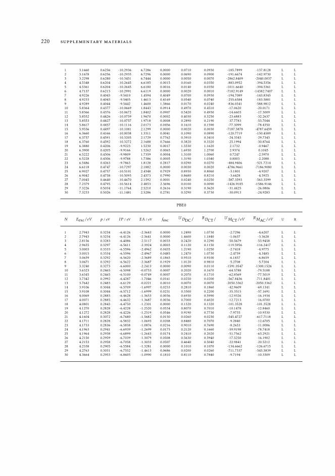
220 supplementary materials
1 3.1660 0.6256 -10.2936 6.7286 0.0000 0.0710 0.0930 -185.7899 -137.8128 L L2 3.1678 0.6256 -10.2935 6.7296 0.0000 0.0690 0.0900 -191.6674 -142.9730 L L3 3.2298 0.6280 -10.3451 6.7444 0.0000 0.0050 0.0070 -2862.8409 -2040.0037 L L4 4.5348 0.6204 -10.2645 6.6185 0.0015 0.0160 0.0350 -883.0952 -394.5356 L L5 4.5361 0.6204 -10.2645 6.6180 0.0016 0.0140 0.0350 -1011.6640 -394.5361 L L6 4.7137 0.6215 -10.2991 6.6119 0.0000 0.0020 0.0010 -7182.9149 -14382.7407 L L7 4.9226 0.4043 -9.5410 1.4594 0.4049 0.0700 0.0930 -194.7089 -143.8345 L L8 4.9233 0.4043 -9.5405 1.4613 0.4169 0.0540 0.0740 -255.6584 -183.5881 L L9 4.9289 0.4044 -9.5442 1.4600 1.3866 0.0170 0.0240 -836.0341 -588.9812 L L10 5.8364 0.4377 -10.0669 1.8443 0.0914 0.4970 0.4510 -17.0620 -20.0171 L L11 5.8366 0.4376 -10.0672 1.8402 0.0907 0.5420 0.4930 -14.6603 -17.3009 L L12 5.8552 0.4426 -10.0759 1.9670 0.0002 0.4030 0.3250 -23.6883 -32.2637 L L13 5.8553 0.4427 -10.0757 1.9718 0.0008 0.2890 0.2190 -37.7783 -53.7044 L L14 5.8617 0.4457 -10.1116 2.0173 0.0456 0.1610 0.1590 -77.3099 -78.4350 L L15 5.9556 0.4497 -10.1081 2.1299 0.0000 0.0020 0.0030 -7187.5878 -4787.6459 L L16 6.3660 0.4166 -10.0038 1.3311 0.0041 0.1090 0.0890 -120.7719 -150.4589 L L17 6.3757 0.4591 -10.3205 2.1729 0.7762 0.3910 0.3410 -24.3343 -29.7343 L L18 6.3760 0.4592 -10.3272 2.1688 0.7666 0.3820 0.3320 -25.1994 -30.8764 L L19 6.3880 0.4206 -9.9223 1.5230 0.0017 1.5530 1.1620 2.1732 -0.9467 L L20 6.3900 0.4205 -9.9166 1.5262 0.0065 1.6930 1.2700 2.9374 0.1045 L L21 6.5222 0.4306 -9.9809 1.7359 0.0004 1.3100 1.0060 0.7247 -2.5970 L L22 6.5228 0.4306 -9.9788 1.7386 0.0005 1.3190 1.0340 0.8003 -2.2088 L L23 6.5486 0.4263 -9.7863 1.8128 0.2817 0.0290 0.0270 -484.9406 -521.7214 L L24 6.6118 0.4747 -10.7297 2.1882 0.0000 0.0030 0.0020 -4786.9661 -7186.9080 L L25 6.9027 0.4757 -10.5101 2.4348 0.7929 0.8930 0.8060 -3.1801 -4.9207 L L26 6.9042 0.4758 -10.5093 2.4373 0.7990 0.8680 0.8210 -3.6428 -4.5925 L L27 7.0045 0.4640 -10.4670 2.1592 0.0001 0.0240 0.0250 -587.3593 -563.3599 L L28 7.2379 0.4795 -10.5614 2.4853 2.3696 0.0100 0.0090 -1426.9185 -1586.9146 L L29 7.3226 0.5034 -11.1764 2.5210 0.2616 0.3190 0.3620 -31.4425 -26.0806 L L30 7.3233 0.5026 -11.1481 2.5286 0.2781 0.3290 0.3730 -30.0913 -24.9283 L L
PBE0
N Eexc/eV p / eV IP / eV EA / eV fosc UDDC/ RDCT/ UMCT/eV RMAC/eV U R
1 2.7943 0.3234 -6.4126 -2.3643 0.0000 1.2490 1.0730 -2.7296 -4.6207 L L2 2.7943 0.3234 -6.4126 -2.3641 0.0000 1.4600 1.1840 -1.0637 -3.3628 L L3 2.8156 0.3283 -6.4086 -2.5117 0.0033 0.2420 0.2290 -50.5679 -53.9458 L L4 2.9655 0.3297 -6.5611 -2.3924 0.0003 0.1120 0.1150 -119.5956 -116.2417 L L5 3.0003 0.3333 -6.5596 -2.4962 0.0435 1.2190 1.0250 -2.7418 -4.9775 L L6 3.0015 0.3334 -6.5596 -2.4967 0.0485 1.2470 1.0730 -2.4759 -4.3485 L L7 3.0659 0.3292 -6.5620 -2.3689 0.1865 0.9510 0.9100 -6.1837 -6.8659 L L8 3.0671 0.3292 -6.5622 -2.3687 0.1929 1.0120 0.9810 -5.2708 -5.7204 L L9 3.3240 0.3273 -6.6000 -2.2413 0.0000 0.0090 0.0110 -1591.0547 -1300.1526 L L10 3.6323 0.2465 -6.5098 -0.0753 0.0007 0.2020 0.1670 -64.5788 -79.5188 L L11 3.6345 0.2465 -6.5100 -0.0749 0.0007 0.2070 0.1710 -62.8569 -77.5019 L L12 3.7342 0.2992 -6.4287 -1.7046 0.0161 0.0250 0.0200 -567.8436 -711.8401 L L13 3.7642 0.2483 -6.6129 -0.0221 0.0010 0.0070 0.0070 -2050.3362 -2050.3362 L L14 3.9106 0.3044 -6.5709 -1.6997 0.0233 0.2810 0.1860 -42.9609 -69.1341 L L15 3.9108 0.3044 -6.5712 -1.6999 0.0231 0.3300 0.2200 -35.3515 -57.1691 L L16 4.0069 0.2883 -6.4628 -1.3653 0.0036 0.6930 0.5990 -12.9326 -16.1934 L L17 4.0071 0.2885 -6.4632 -1.3687 0.0036 0.7000 0.6020 -12.7213 -16.0700 L L18 4.0801 0.2843 -6.4750 -1.2301 0.0000 0.1320 0.1320 -101.3528 -101.3528 L L19 4.1270 0.2828 -6.4228 -1.2520 0.0534 0.8070 0.7010 -10.1478 -12.8460 L L20 4.1272 0.2828 -6.4226 -1.2519 0.0546 0.9190 0.7730 -7.9735 -10.9330 L L21 4.1604 0.3072 -6.7680 -1.5682 0.0150 0.0260 0.0230 -545.4727 -617.7118 L L22 4.1711 0.2828 -6.5832 -1.0693 0.0208 0.8480 0.7070 -9.2840 -12.6705 L L23 4.1733 0.2836 -6.5858 -1.0876 0.0216 0.9010 0.7690 -8.2653 -11.0086 L L24 4.1963 0.2941 -6.6939 -1.2699 0.0175 0.2120 0.1660 -59.9198 -78.7418 L L25 4.1964 0.2938 -6.6899 -1.2643 0.0174 0.2410 0.2020 -51.7562 -63.2921 L L26 4.2150 0.2959 -6.7039 -1.3079 0.0508 0.5630 0.5940 -17.5250 -16.1902 L L27 4.2153 0.2958 -6.7058 -1.3033 0.0507 0.4640 0.5040 -22.9841 -20.5212 L L28 4.2338 0.2905 -6.5584 -1.3281 0.0000 0.1010 0.1070 -134.6662 -126.6715 L L29 4.2763 0.3031 -6.7552 -1.4613 0.0686 0.0200 0.0260 -711.7337 -545.5839 L L30 4.3664 0.2953 -6.8605 -1.0990 0.1810 0.8110 0.7840 -9.7194 -10.3309 L L
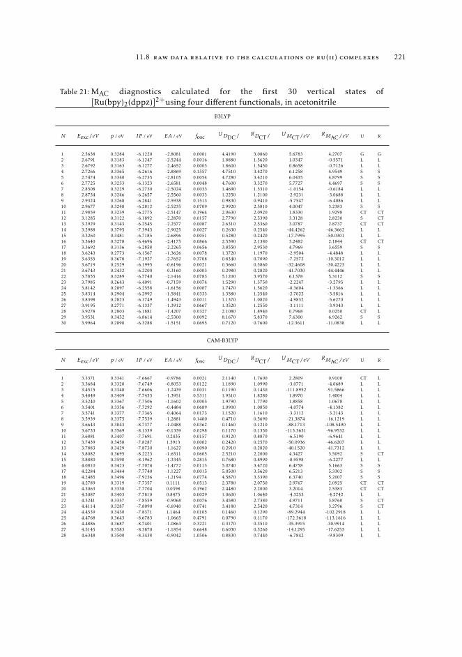
11.8 raw data relative to the calculations of ru(ii) complexes 221
Table 21: MAC diagnostics calculated for the first 30 vertical states of[Ru(bpy)2(dppz)]2+using four different functionals, in acetonitrile
B3LYP
N Eexc/eV p / eV IP / eV EA / eV fosc UDDC/ RDCT/ UMCT/eV RMAC/eV U R
1 2.5638 0.3284 -6.1220 -2.8081 0.0001 4.4190 3.0860 5.6783 4.2707 G G2 2.6791 0.3183 -6.1247 -2.5244 0.0016 1.8880 1.5620 1.0347 -0.5571 L L3 2.6792 0.3163 -6.1277 -2.4652 0.0003 1.8600 1.5450 0.8658 -0.7126 L L4 2.7266 0.3365 -6.2616 -2.8869 0.1557 4.7510 3.4270 6.1258 4.9549 S S5 2.7474 0.3340 -6.2735 -2.8105 0.0054 4.7280 3.4210 6.0435 4.8799 S S6 2.7725 0.3233 -6.1323 -2.6581 0.0048 4.7600 3.3270 5.7727 4.4697 S S7 2.8508 0.3229 -6.2730 -2.5024 0.0033 1.4690 1.5310 -1.0154 -0.6184 L L8 2.8734 0.3246 -6.2657 -2.5560 0.0033 1.2250 1.2100 -2.9231 -3.0688 L L9 2.9324 0.3268 -6.2841 -2.5938 0.1513 0.9830 0.9410 -5.7547 -6.4086 L L10 2.9677 0.3240 -6.2812 -2.5235 0.0709 2.9920 2.5810 4.0047 3.2383 S S11 2.9859 0.3239 -6.2775 -2.5147 0.1964 2.0630 2.0920 1.8330 1.9298 CT CT12 3.1285 0.3122 -6.1892 -2.2870 0.0157 2.7790 2.5390 3.3128 2.8230 S CT13 3.2929 0.3143 -6.2545 -2.2577 0.0087 2.6310 2.5360 3.0787 2.8737 CT CT14 3.2988 0.3795 -7.3943 -2.9025 0.0027 0.2630 0.2540 -44.4262 -46.3662 L L15 3.3260 0.3481 -6.7185 -2.6896 0.0051 0.5280 0.2420 -17.7995 -50.0301 L L16 3.3640 0.3278 -6.4696 -2.4175 0.0866 2.5390 2.1380 3.2482 2.1844 CT CT17 3.3692 0.3136 -6.2858 -2.2265 0.0656 3.8550 2.9530 4.7969 3.6559 S S18 3.6243 0.2773 -6.1567 -1.3626 0.0078 1.3720 1.1970 -2.9504 -4.4848 L L19 3.6355 0.3678 -7.1927 -2.7652 0.3708 0.8340 0.7090 -7.2572 -10.3012 L L20 3.6719 0.2529 -6.1995 -0.6196 0.0021 0.3660 0.3860 -32.4608 -30.4223 L L21 3.6743 0.2432 -6.2200 -0.3160 0.0003 0.2980 0.2820 -41.7030 -44.4446 L L22 3.7855 0.3289 -6.7740 -2.1416 0.0783 5.1200 3.9570 6.1378 5.3112 S S23 3.7985 0.2643 -6.4091 -0.7159 0.0074 1.5290 1.3750 -2.2247 -3.2795 L L24 3.8142 0.2897 -6.2558 -1.6156 0.0007 1.7470 1.5620 -0.3604 -1.3366 L L25 3.8314 0.2904 -6.2992 -1.5841 0.0333 1.3580 1.2540 -2.7022 -3.5816 L L26 3.8398 0.2823 -6.1749 -1.4943 0.0011 1.1370 1.0820 -4.9832 -5.6270 L L27 3.9195 0.2771 -6.1337 -1.3912 0.0667 1.3520 1.2550 -3.1111 -3.9343 L L28 3.9278 0.2803 -6.1881 -1.4207 0.0327 2.1080 1.8940 0.7968 0.0250 CT L29 3.9531 0.3452 -6.8614 -2.5300 0.0092 8.1670 5.8370 7.6300 6.9262 S S30 3.9964 0.2890 -6.3288 -1.5151 0.0695 0.7120 0.7600 -12.3611 -11.0838 L L
CAM-B3LYP
N Eexc/eV p / eV IP / eV EA / eV fosc UDDC/ RDCT/ UMCT/eV RMAC/eV U R
1 3.3371 0.3341 -7.6667 -0.9786 0.0021 2.1140 1.7600 2.2809 0.9108 CT L2 3.3684 0.3320 -7.6749 -0.8053 0.0122 1.1890 1.0990 -3.0771 -4.0689 L L3 3.4515 0.3348 -7.6606 -1.2439 0.0031 0.1190 0.1430 -111.8952 -91.5866 L L4 3.4849 0.3409 -7.7433 -1.3951 0.5311 1.9510 1.8280 1.8970 1.4004 L L5 3.5240 0.3367 -7.7506 -1.1602 0.0005 1.9790 1.7790 1.8858 1.0678 L L6 3.5401 0.3356 -7.7292 -0.4484 0.0689 1.0900 1.0850 -4.0774 -4.1382 L L7 3.5741 0.3377 -7.7365 -0.4064 0.0173 1.1520 1.1610 -3.3112 -3.2143 L L8 3.5939 0.3375 -7.7539 -1.2881 0.1400 0.4710 0.5690 -21.3874 -16.1219 L L9 3.6643 0.3843 -8.7377 -1.0488 0.0362 0.1460 0.1210 -88.1713 -108.5490 L L10 3.6733 0.3569 -8.1339 -0.1339 0.0298 0.1170 0.1350 -113.3631 -96.9532 L L11 3.6881 0.3407 -7.7691 0.2435 0.0157 0.9120 0.8870 -6.5190 -6.9641 L L12 3.7439 0.3458 -7.8287 1.3913 0.0002 0.2420 0.2570 -50.0936 -46.6207 L L13 3.7883 0.3429 -7.8730 -1.1622 0.0090 0.2910 0.2820 -40.1520 -41.7312 L L14 3.8082 0.3695 -8.2223 -1.6511 0.0605 2.5210 2.2000 4.3427 3.5092 S CT15 3.8880 0.3598 -8.1962 -1.3345 0.2815 0.7680 0.8990 -8.9598 -6.2277 L L16 4.0810 0.3423 -7.7074 -1.4772 0.0113 5.0740 3.4720 6.4758 5.1663 S S17 4.2284 0.3444 -7.7740 -1.1227 0.0015 5.0500 3.5620 6.5213 5.3302 S S18 4.2485 0.3496 -7.9236 -1.2194 0.0774 4.5870 3.3390 6.3740 5.2007 S S19 4.2789 0.3319 -7.7357 0.1111 0.0513 2.3780 2.0750 2.9767 2.0925 CT CT20 4.3063 0.3338 -7.7704 0.0398 0.1962 2.4480 2.2000 3.2014 2.5383 CT CT21 4.3087 0.3403 -7.7810 0.8475 0.0029 1.0600 1.0640 -4.3253 -4.2742 L L22 4.3241 0.3357 -7.8559 -0.9068 0.0076 3.4580 2.7380 4.9711 3.8760 S CT23 4.4114 0.3287 -7.8090 -0.6940 0.0741 3.4180 2.5420 4.7314 3.2796 S CT24 4.4539 0.3430 -7.8371 1.1464 0.0105 0.1460 0.1290 -89.2944 -102.2918 L L25 4.4768 0.3643 -8.6783 -1.0665 0.4791 0.0790 0.1170 -172.3618 -113.1616 L L26 4.4886 0.3687 -8.7401 -1.0863 0.3221 0.3170 0.3510 -35.3915 -30.9914 L L27 4.5145 0.3583 -8.3870 -1.1854 0.6648 0.6030 0.5260 -14.1295 -17.6253 L L28 4.6348 0.3500 -8.3438 -0.9042 1.0506 0.8830 0.7440 -6.7842 -9.8309 L L
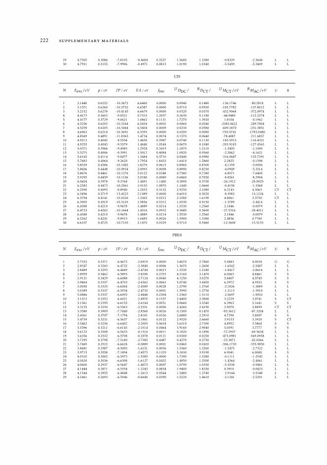
222 supplementary materials
29 4.7505 0.3086 -7.8105 -0.4684 0.3527 1.5600 1.3380 -0.8329 -2.3644 L L30 4.7931 0.3155 -7.9906 -0.4971 0.0815 1.0190 1.0340 -5.5459 -5.3409 L L
CIS
N Eexc/eV p / eV IP / eV EA / eV fosc UDDC/ RDCT/ UMCT/eV RMAC/eV U R
1 3.1440 0.6252 -10.3672 6.6460 0.0000 0.0940 0.1480 -136.1746 -80.2818 L L2 3.1571 0.6260 -10.3752 6.6587 0.0000 0.0710 0.0930 -185.7782 -137.8012 L L3 3.2132 0.6278 -10.4145 6.6679 0.0000 0.0320 0.0370 -432.9068 -372.0974 L L4 4.4173 0.3603 -9.0521 0.7515 1.2037 0.2630 0.1180 -44.9480 -112.2274 L L5 4.4177 0.3729 -9.0621 1.0862 0.1131 1.7270 1.3920 1.8104 -0.1962 L L6 4.5256 0.6203 -10.3344 6.5454 0.0002 0.0060 0.0540 -2383.0622 -249.7804 L L7 4.5259 0.6205 -10.3444 6.5404 0.0009 0.0230 0.0580 -609.1870 -231.3851 L L8 4.6963 0.6214 -10.3691 6.5393 0.0000 0.0200 0.0080 -703.0741 -1783.0480 L L9 4.8569 0.4891 -11.8365 1.4724 0.0074 0.1570 0.0640 -78.4087 -211.6857 L L10 4.9213 0.4042 -9.5554 1.4430 0.3987 0.0740 0.1130 -183.5915 -116.4321 L L11 4.9255 0.4043 -9.5579 1.4440 1.0544 0.0670 0.1040 -203.9183 -127.4563 L L12 5.0371 0.3966 -9.4983 1.2924 0.3419 1.1870 1.2110 -1.3405 -1.1000 L L13 5.3275 0.4006 -9.3991 1.5012 0.4084 1.0920 0.9560 -2.2862 -4.1621 L L14 5.6165 0.4114 -9.8477 1.3484 0.3710 0.0440 0.0980 -316.0687 -135.7391 L L15 5.7683 0.4064 -9.2620 1.7954 1.8433 1.6410 1.2860 2.2825 -0.1398 L L16 5.8539 0.4386 -10.1082 1.8270 0.0615 0.8960 0.8500 -4.1359 -5.0056 L L17 5.8606 0.4448 -10.0934 2.0093 0.0008 0.8890 0.8250 -4.0949 -5.3514 L L18 5.8676 0.4461 -10.1276 2.0122 0.0248 0.7580 0.7280 -6.8571 -7.6400 L L19 5.9295 0.4459 -10.1106 2.0240 0.0089 0.6860 0.7050 -8.8561 -8.2904 L L20 6.0604 0.3978 -9.3768 1.4491 1.1400 0.3890 0.3700 -26.1912 -28.0920 L L21 6.2582 0.4473 -10.2561 1.9152 1.0870 1.1440 1.0660 -0.4158 -1.3368 L L22 6.2590 0.4093 -9.8940 1.2433 0.3152 2.9250 2.1080 6.2143 4.3063 CT CT23 6.3496 0.5719 -13.4523 2.1089 0.0000 0.6010 0.5020 -8.3983 -13.1234 L L24 6.3794 0.4141 -10.0326 1.2365 0.0212 2.2280 1.6190 4.8061 2.3750 CT L25 6.3905 0.4519 -10.3103 1.9856 0.5312 1.0530 0.9150 -1.3789 -3.4414 L L26 6.4388 0.4210 -9.9678 1.4889 0.0214 1.5530 1.2560 2.1846 -0.0079 L L27 6.4723 0.4262 -10.1664 1.4316 0.0932 0.3680 0.3600 -27.5316 -28.4011 L L28 6.4388 0.4210 -9.9678 1.4889 0.0214 1.5530 1.2560 2.1846 -0.0079 L L29 6.5262 0.4241 -9.8915 1.6485 0.0026 1.5900 1.3380 2.4836 0.7780 L L30 6.6107 0.4725 -10.7105 2.1470 0.0329 0.5710 0.5460 -12.3608 -13.5155 L L
PBE0
N Eexc/eV p / eV IP / eV EA / eV fosc UDDC/ RDCT/ UMCT/eV RMAC/eV U R
1 2.7353 0.3371 -6.4672 -2.6919 0.0000 3.8670 2.7860 5.4483 4.0034 G G2 2.8347 0.3263 -6.4732 -2.3840 0.0006 1.3670 1.2600 -1.6542 -2.5487 L L3 2.8489 0.3293 -6.4689 -2.4744 0.0013 1.3330 1.2180 -1.8417 -2.8616 L L4 2.8959 0.3462 -6.5893 -2.8200 0.2253 4.2160 3.1470 6.0063 4.8461 S S5 2.9121 0.3429 -6.6088 -2.7124 0.0040 4.1250 3.0270 5.8407 4.5745 S S6 2.9864 0.3357 -6.4703 -2.6562 0.0063 5.0740 3.4450 6.2972 4.9553 S S7 3.0050 0.3335 -6.6004 -2.4589 0.0028 1.2790 1.3760 -2.1826 -1.3889 L L8 3.0389 0.3337 -6.5934 -2.4735 0.0001 1.3990 1.3750 -1.2113 -1.3910 L L9 3.0886 0.3337 -6.6093 -2.4448 0.2304 1.2360 1.3110 -2.5697 -1.9032 L L10 3.1513 0.3353 -6.6021 -2.4970 0.1537 2.4400 2.3800 3.2229 3.0741 S CT11 3.1561 0.3395 -6.6155 -2.6144 0.0051 5.0660 3.5340 6.3963 5.1641 S S12 3.3135 0.3250 -6.5563 -2.2551 0.0096 2.4260 2.4190 2.9070 2.8899 CT CT13 3.3580 0.3909 -7.7440 -2.8560 0.0026 0.1500 0.1470 -85.3612 -87.3204 L L14 3.4361 0.3707 -7.1794 -2.8181 0.0326 2.6880 2.2910 4.7290 3.8007 S S15 3.4759 0.3231 -6.5637 -2.1861 0.0122 2.9520 2.6660 3.9153 3.3920 S CT16 3.5462 0.3256 -6.6402 -2.2005 0.0654 3.6310 2.7300 4.8952 3.5864 S S17 3.5596 0.3211 -6.6143 -2.1014 0.0464 3.9160 2.9040 5.0591 3.7777 S S18 3.6122 0.2508 -6.5633 -0.1510 0.0011 0.1820 0.1890 -72.2937 -69.3634 L L19 3.6356 0.2532 -6.5708 -0.2078 0.0121 0.0300 0.0250 -473.0981 -569.0958 L L20 3.7295 0.3798 -7.5180 -2.7585 0.4487 0.4270 0.2750 -23.3871 -42.0266 L L21 3.7469 0.2522 -6.6624 -0.0889 0.0001 0.0460 0.0420 -306.1720 -335.9850 L L22 3.8681 0.2987 -6.5005 -1.6151 0.0056 1.5360 1.3260 -1.2475 -2.7322 L L23 3.9715 0.3558 -7.1894 -2.4573 0.1329 5.1830 3.9190 6.9041 6.0080 S S24 4.0310 0.3002 -6.5973 -1.5585 0.0000 1.7390 1.5280 -0.1111 -1.2545 L L25 4.0430 0.3036 -6.6308 -1.6127 0.0432 1.4850 1.3500 -1.4364 -2.4061 L L26 4.0600 0.2937 -6.5647 -1.4073 0.0007 1.0790 1.0330 -5.3538 -5.9481 L L27 4.1444 0.2871 -6.5554 -1.2243 0.0834 1.9400 1.8330 0.3910 -0.0423 L L28 4.1544 0.2855 -6.4848 -1.2613 0.0544 1.3480 1.2740 -2.9144 -3.5348 L L29 4.1861 0.2693 -6.5946 -0.6640 0.0290 1.5220 1.4610 -2.1341 -2.5291 L L
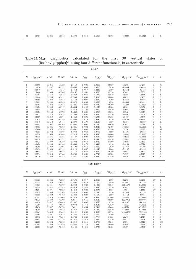
11.8 raw data relative to the calculations of ru(ii) complexes 223
30 4.1971 0.3085 -6.8043 -1.5598 0.0515 0.6560 0.7190 -13.5557 -11.6323 L L
Table 22: MAC diagnostics calculated for the first 30 vertical states of[Ru(bpy)2(tpphz)]2+using four different functionals, in acetonitrile
B3LYP
N Eexc/eV p / eV IP / eV EA / eV fosc UDDC/ RDCT/ UMCT/eV RMAC/eV U R
1 2.5898 0.3255 -6.1328 -2.7163 0.0001 3.8110 2.8050 5.0795 3.7244 G G2 2.6836 0.3167 -6.1372 -2.4656 0.0000 1.3810 1.2830 -1.8094 -2.6059 L L3 2.6840 0.3191 -6.1343 -2.5364 0.0017 1.4480 1.3180 -1.2614 -2.2423 L L4 2.7640 0.3343 -6.2708 -2.8152 0.2601 4.0500 3.1510 5.5403 4.5259 S S5 2.7764 0.3313 -6.2845 -2.7243 0.0061 4.1390 3.1510 5.5368 4.4459 S S6 2.8040 0.3253 -6.1411 -2.7065 0.0045 5.4060 3.7800 6.1893 5.0435 S S7 2.8565 0.3238 -6.2824 -2.5174 0.0037 1.4290 1.5290 -1.2657 -0.6066 L L8 2.8821 0.3249 -6.2743 -2.5570 0.0009 1.0520 1.0790 -4.8466 -4.5041 L L9 2.9461 0.3254 -6.2923 -2.5421 0.2030 0.5780 0.6790 -16.0586 -12.3529 L L10 2.9874 0.3285 -6.2917 -2.6404 0.0192 5.1050 3.7180 6.1181 5.0658 S S11 2.9948 0.3254 -6.2754 -2.5614 0.1146 3.2310 3.0820 4.3968 4.1813 S S12 3.0074 0.3165 -6.1578 -2.4449 0.0631 4.0260 3.1010 5.0348 3.9679 S S13 3.1877 0.3212 -6.2938 -2.4404 0.0301 4.5130 3.3320 5.5509 4.4200 S S14 3.1887 0.3219 -6.2891 -2.4568 0.0495 4.6230 3.3630 5.6455 4.4785 S S15 3.2678 0.3205 -6.3140 -2.3469 0.0173 1.6480 1.8310 -0.0159 0.8574 L L16 3.4048 0.3610 -6.9441 -2.8299 0.6599 1.4680 1.3550 0.0151 -0.8029 L L17 3.4091 0.3607 -6.9263 -2.8480 0.0091 4.1560 3.4650 6.3497 5.6588 S S18 3.5003 0.3826 -7.5373 -2.8446 0.0032 0.2020 0.2480 -60.8731 -47.6508 L L19 3.5680 0.3676 -7.1478 -2.8491 0.0000 4.8580 3.5190 7.0376 5.9097 G G20 3.6273 0.2754 -6.1705 -1.2938 0.0068 1.2910 1.1550 -3.6601 -4.9735 L L21 3.6728 0.2560 -6.2048 -0.7015 0.0029 0.4590 0.4860 -24.4061 -22.6633 L L22 3.6735 0.2436 -6.2286 -0.3187 0.0008 0.3080 0.2950 -40.1233 -42.1836 L L23 3.7958 0.2473 -6.3297 -0.3227 0.0011 0.2440 0.2410 -52.2843 -53.0189 L L24 3.8077 0.3399 -6.8279 -2.3984 0.0313 5.0720 4.4190 6.4088 5.9893 S S25 3.2678 0.3205 -6.3140 -2.3469 0.0173 1.6480 1.8310 -0.0158 0.8574 L L26 3.8365 0.2920 -6.3091 -1.6198 0.0311 1.3550 1.2670 -2.6817 -3.4198 L L27 3.8434 0.2836 -6.1922 -1.5116 0.0007 1.1140 1.0860 -5.2102 -5.5435 L L28 3.8644 0.3437 -6.9025 -2.4110 1.0270 4.4290 3.8280 6.1001 5.5897 S S29 3.8754 0.3513 -6.9966 -2.5255 0.0086 6.7740 5.0580 7.4327 6.7115 S S30 3.9220 0.3363 -6.8142 -2.3041 0.2402 5.5390 4.7130 6.5519 6.0963 S S
CAM-B3LYP
N Eexc/eV p / eV IP / eV EA / eV fosc UDDC/ RDCT/ UMCT/eV RMAC/eV U R
1 3.3362 0.3345 -7.6757 -0.9695 0.0017 2.0950 1.7590 2.2292 0.9163 CT L2 3.3715 0.3326 -7.6852 -0.8000 0.0218 1.1570 1.0850 -3.3951 -4.2210 L L3 3.4560 0.3351 -7.6699 -1.2332 0.0043 0.1300 0.1540 -101.6473 -84.3850 L L4 3.4714 0.3422 -7.7583 -1.4414 0.7626 1.5880 1.5730 0.2442 0.1578 L L5 3.5254 0.3371 -7.7582 -1.1418 0.0005 2.0070 1.8030 1.9974 1.1856 CT L6 3.5429 0.3359 -7.7369 -0.4513 0.0690 1.1590 1.1510 -3.2846 -3.3710 L L7 3.5757 0.3382 -7.7472 -0.3340 0.0239 1.1690 1.2000 -3.1163 -2.7981 L L8 3.5997 0.3378 -7.7603 -1.2819 0.1381 0.4850 0.5860 -20.4988 -15.3816 L L9 3.6725 0.3403 -7.7708 0.3811 0.0655 0.0620 0.0580 -222.9912 -239.0086 L L10 3.6838 0.3427 -7.8083 -0.1397 0.0682 1.0550 1.0330 -4.3237 -4.6143 L L11 3.7366 0.3517 -7.9810 -1.0832 0.1718 0.2640 0.2670 -44.9732 -44.3603 L L12 3.7438 0.3457 -7.8376 1.3689 0.0004 0.2460 0.2640 -49.1270 -45.1360 L L13 3.8285 0.3400 -7.8542 -1.1012 0.1689 0.1490 0.1870 -87.3896 -67.7511 L L14 3.8863 0.4038 -9.2642 -1.5121 0.0045 0.0130 0.0510 -1096.6777 -271.3583 L L15 4.0098 0.3591 -8.1635 -1.4627 0.0170 1.7270 1.5200 1.4345 0.2990 L L16 4.1538 0.3413 -7.7634 -1.3705 0.0353 4.7710 3.4820 6.2692 5.1519 S S17 4.1642 0.3295 -7.7136 -1.1317 0.1014 3.5820 2.7120 4.9472 3.6576 S CT18 4.2275 0.3394 -7.8218 -1.2219 0.0611 3.0790 2.5240 4.5594 3.5310 S CT19 4.2495 0.3340 -7.7859 -0.4846 0.1174 3.3480 2.6490 4.7889 3.6540 S CT20 4.2873 0.3449 -7.8432 -0.6186 0.1416 4.0720 3.2480 5.8479 4.9508 S S
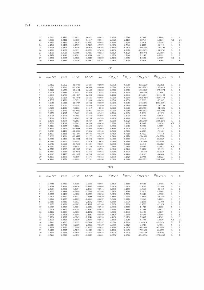
224 supplementary materials
21 4.2902 0.3432 -7.7832 0.6621 0.0072 1.9000 1.7660 1.7591 1.1840 L L22 4.3351 0.3411 -7.8060 0.1417 0.0011 2.6720 2.4130 3.8919 3.3134 CT CT23 4.3451 0.3415 -7.7628 -0.8590 0.0042 4.8140 3.5200 6.3014 5.2018 S S24 4.4268 0.3482 -8.1515 -0.2468 0.5572 0.8050 0.7840 -8.4127 -8.8919 L L25 4.4706 0.3475 -8.1046 0.0963 0.6192 0.1530 0.1170 -84.6606 -113.6192 L L26 4.4791 0.3652 -8.6931 -1.0736 0.5639 0.1030 0.0870 -129.8653 -155.5761 L L27 4.4901 0.3664 -8.6498 -0.9137 0.0553 0.3620 0.4020 -29.8074 -25.8494 L L28 4.5478 0.3640 -8.4281 -1.3281 0.0222 1.8750 1.5660 2.2245 0.7091 L L29 4.5598 0.3685 -8.8808 -0.9243 0.0000 2.5290 1.9650 4.3332 2.6989 CT L30 4.6119 0.3564 -8.4136 -1.0962 0.0261 3.2800 2.9440 5.3079 4.8068 S S
CIS
N Eexc/eV p / eV IP / eV EA / eV fosc UDDC/ RDCT/ UMCT/eV RMAC/eV U R
1 3.1432 0.6252 -10.3700 6.6421 0.0000 0.0930 0.1500 -137.8229 -78.9856 L L2 3.1563 0.6260 -10.3791 6.6546 0.0000 0.0710 0.0930 -185.7783 -137.8013 L L3 3.2128 0.6278 -10.4184 6.6640 0.0000 0.0320 0.0370 -432.9067 -372.0974 L L4 4.2729 0.3493 -8.7014 0.8033 1.5452 0.4300 0.3930 -23.9829 -27.1357 L L5 4.5242 0.5789 -10.1317 5.6208 0.0008 0.1110 0.0440 -113.9741 -311.5123 L L6 4.5243 0.6204 -10.3378 6.5446 0.0007 0.0050 0.0540 -2863.0479 -249.7778 L L7 4.5337 0.4238 -9.3059 2.2268 0.0053 0.8560 0.8330 -5.2893 -5.7537 L L8 4.6958 0.6213 -10.3727 6.5344 0.0000 0.0190 0.0080 -740.9693 -1783.0494 L L9 4.9214 0.4042 -9.5578 1.4408 0.3980 0.0750 0.1150 -180.9968 -114.2158 L L10 4.9257 0.4043 -9.5603 1.4419 1.0542 0.0680 0.1060 -200.7574 -124.8435 L L11 5.0571 0.4995 -11.9950 1.5961 0.0103 0.0300 0.0360 -466.3973 -386.3992 L L12 5.0751 0.4017 -9.5402 1.3909 0.3422 0.7860 0.8950 -7.3891 -5.1579 L L13 5.2039 0.3901 -9.2585 1.3576 0.3007 1.5760 1.4030 1.4792 0.3526 L L14 5.4344 0.4020 -9.1269 1.8133 0.4783 0.8830 0.6440 -5.3674 -11.4195 L L15 5.4545 0.4094 -9.2687 1.8727 1.9891 0.0360 0.0020 -388.8489 -7188.6845 L L16 5.6501 0.4018 -9.3142 1.6200 0.0638 2.2710 1.9670 4.5935 3.6136 CT L17 5.8464 0.3987 -9.4786 1.3699 0.6901 1.8900 1.6070 3.2296 1.8879 L L18 5.8545 0.4373 -10.0898 1.8098 0.1063 0.8160 0.7920 -5.7470 -6.2818 L L19 5.8573 0.4439 -10.0901 1.9886 0.1148 0.7680 0.7410 -6.6709 -7.3541 L L20 5.8677 0.4461 -10.1299 2.0103 0.0250 0.7630 0.7350 -6.7322 -7.4512 L L21 5.9092 0.4396 -10.0453 1.9172 0.2613 0.3460 0.3770 -29.6550 -26.2328 L L22 5.9686 0.5454 -11.8024 3.0384 0.0000 1.0360 0.5600 0.9415 -10.8729 L L23 6.0484 0.4102 -9.4014 1.7616 1.6652 0.5610 0.5790 -14.5048 -13.7068 L L24 6.1783 0.5551 -11.9519 3.1521 0.0201 0.9950 0.5520 0.6319 -10.9824 L L25 6.2543 0.4120 -9.8974 1.3150 0.3079 2.7440 2.0100 5.9647 4.0483 CT CT26 6.2772 0.4503 -10.2965 1.9581 0.0751 0.8060 0.8160 -5.6110 -5.3921 L L27 6.3814 0.4169 -10.0072 1.3376 0.0652 0.6260 0.5420 -11.6578 -15.2228 L L28 6.3895 0.4473 -10.2922 1.8785 0.4744 0.8980 0.8100 -3.8645 -5.6066 L L29 6.4377 0.4198 -9.9669 1.4575 0.0152 1.5770 1.2820 2.2934 0.1922 L L30 6.4449 0.4271 -9.8999 1.7231 0.0996 0.0900 0.0480 -148.3731 -288.3697 L L
PBE0
N Eexc/eV p / eV IP / eV EA / eV fosc UDDC/ RDCT/ UMCT/eV RMAC/eV U R
1 2.7488 0.3350 -6.4788 -2.6215 0.0001 3.4520 2.5850 4.9441 3.5450 G G2 2.8396 0.3269 -6.4836 -2.3892 0.0004 1.3650 1.2750 -1.6541 -2.3988 L L3 2.8554 0.3301 -6.4794 -2.4867 0.0016 1.3470 1.2490 -1.7070 -2.5458 L L4 2.9207 0.3444 -6.5999 -2.7568 0.3504 3.5820 2.8660 5.3512 4.3469 S S5 2.9287 0.3408 -6.6210 -2.6389 0.0038 3.6290 2.7790 5.3046 4.0910 S S6 3.0120 0.3342 -6.6077 -2.4688 0.0029 1.1610 1.2940 -3.3100 -2.0353 L L7 3.0260 0.3375 -6.4823 -2.6964 0.0057 5.5620 3.8270 6.5960 5.4223 S S8 3.0461 0.3340 -6.6033 -2.4692 0.0063 1.3910 1.3970 -1.2645 -1.2200 L L9 3.0952 0.3338 -6.6185 -2.4367 0.2344 1.3050 1.3820 -1.9522 -1.3374 L L10 3.1669 0.3367 -6.6084 -2.5280 0.0942 2.8990 2.8450 4.1943 4.1000 S S11 3.1926 0.3420 -6.6214 -2.6780 0.0022 5.7180 3.9860 6.7869 5.6927 S S12 3.2102 0.3280 -6.5003 -2.4172 0.0228 4.3450 3.2640 5.6125 4.5149 S S13 3.3736 0.3328 -6.6194 -2.4180 0.0549 4.4820 3.2600 5.8433 4.6390 S S14 3.3796 0.3317 -6.6249 -2.3844 0.0320 4.1630 3.1790 5.5667 4.4961 S S15 3.4275 0.3326 -6.6579 -2.3299 0.0015 2.4530 2.5280 3.1798 3.3539 CT CT16 3.5112 0.3705 -7.2327 -2.7961 0.7197 0.6580 0.5220 -11.8014 -17.5030 L L17 3.5487 0.3711 -7.2359 -2.8163 0.0120 3.8980 3.3120 6.4040 5.7504 S S18 3.5708 0.3950 -7.9098 -2.8005 0.0032 0.1380 0.1830 -93.5966 -67.9379 L L19 3.6112 0.2517 -6.5745 -0.1646 0.0013 0.1860 0.1950 -70.5684 -66.9953 L L20 3.6330 0.2516 -6.5818 -0.1507 0.0033 0.1720 0.1670 -76.8729 -79.3795 L L21 3.7461 0.2528 -6.6732 -0.0928 0.0001 0.0550 0.0520 -254.9336 -270.0382 L L

11.8 raw data relative to the calculations of ru(ii) complexes 225
22 3.7747 0.3799 -7.5322 -2.7958 0.0000 4.6600 3.4400 7.2470 6.1511 G G23 3.8734 0.2993 -6.5119 -1.6219 0.0055 1.5110 1.3230 -1.3845 -2.7387 L L24 3.9832 0.3583 -7.2615 -2.4534 0.2798 5.5050 4.3490 7.1348 6.4395 S S25 4.0145 0.3557 -7.2412 -2.4015 0.8311 5.0470 4.1910 6.8273 6.2445 S S26 4.0308 0.3649 -7.3793 -2.4899 0.0788 4.4710 3.7060 6.7094 6.0446 S S27 4.0308 0.3649 -7.3793 -2.4899 0.0788 4.4710 3.7060 6.7094 6.0446 S S28 4.0308 0.3649 -7.3793 -2.4899 0.0788 4.4710 3.7060 6.7094 6.0446 S S29 4.0645 0.2944 -6.5771 -1.4140 0.0002 1.0680 1.0440 -5.4723 -5.7823 L L30 4.0347 0.3012 -6.6125 -1.5692 0.0054 1.7860 1.5790 0.1331 -0.9239 L L
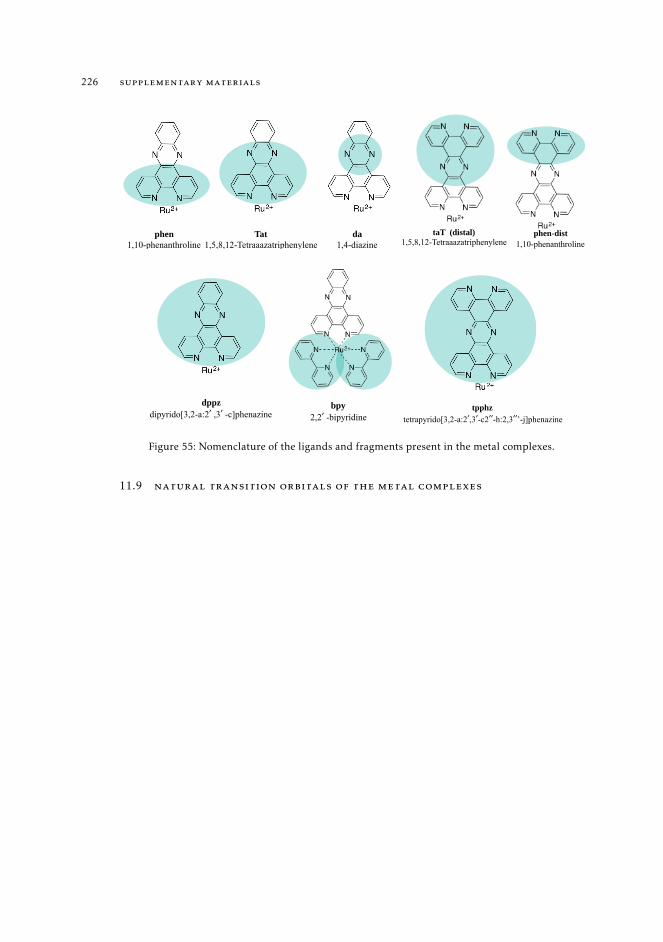
226 supplementary materials
phen 1,10-phenanthroline
Tat 1,5,8,12-Tetraaazatriphenylene
da 1,4-diazine
taT (distal) 1,5,8,12-Tetraaazatriphenylene
phen-dist 1,10-phenanthroline
dppz dipyrido[3,2-a:2′ ,3′ -c]phenazine
bpy 2,2′ -bipyridine
tpphz tetrapyrido[3,2-a:2′,3′-c2′′-h:2,3′′’-j]phenazine
Figure 55: Nomenclature of the ligands and fragments present in the metal complexes.
11.9 natural transition orbitals of the metal complexes
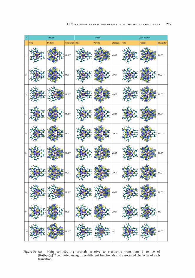
11.9 natural transition orbitals of the metal complexes 227
N B3LYP PBE0 CAM-B3LYP
Hole Particle Character Hole Particle Character Hole Particle Character
1 MLCT MLCT MLCT
2 MLCT MLCT MLCT
3 MLCT MLCT MLCT
4 MLCT MLCT MLCT
5 MLCT MLCT MLCT
6 MLCT MLCT MLCT
7 MLCT MLCT MLCT
8 MLCT MLCT MLCT
9 MLCT MLCT MC
10 MLCT MC MLCT
Figure 56: (a) Main contributing orbitals relative to electronic transitions 1 to 10 of[Ru(bpy)3]2+computed using three different functionals and associated character of eachtransition.
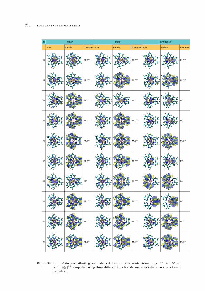
228 supplementary materials
/
N B3LYP PBE0 CAM-B3LYP
Hole Particle Character Hole Particle Character Hole Particle Character
11 MLCT MLCT MLCT
12 MLCT MLCT MLCT
13 MLCT MC MC
14 MLCT MLCT MC
15 MLCT MLCT MLCT
16 MLCT MLCT MC
17 MC MLCT LC
18 MLCT MLCT LC
19 MLCT MLCT MLCT
20 MLCT MLCT MLCT
Figure 56: (b) Main contributing orbitals relative to electronic transitions 11 to 20 of[Ru(bpy)3]2+computed using three different functionals and associated character of eachtransition.
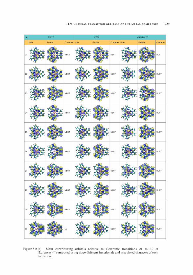
11.9 natural transition orbitals of the metal complexes 229
N B3LYP PBE0 CAM-B3LYP
Hole Particle Character Hole Particle Character Hole Particle Character
21 MLCT MLCT MLCT
22 MLCT MLCT MLCT
23 MLCT MLCT MLCT
24 MLCT MLCT MLCT
25 MLCT MLCT MLCT
26 MLCT MLCT MLCT
27 MLCT MLCT MLCT
28 MLCT MLCT MLCT
29 MLCT MLCT MLCT
30 LC MLCT MLCT
Figure 56: (c) Main contributing orbitals relative to electronic transitions 21 to 30 of[Ru(bpy)3]2+computed using three different functionals and associated character of eachtransition.
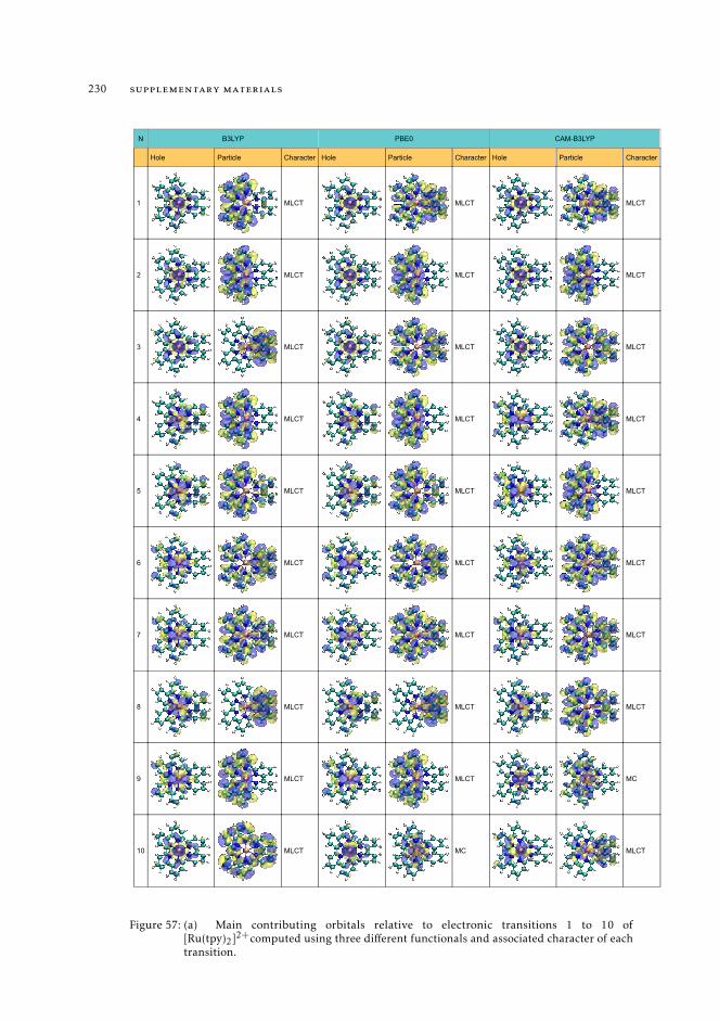
230 supplementary materials
N B3LYP PBE0 CAM-B3LYP
Hole Particle Character Hole Particle Character Hole Particle Character
1 MLCT MLCT MLCT
2 MLCT MLCT MLCT
3 MLCT MLCT MLCT
4 MLCT MLCT MLCT
5 MLCT MLCT MLCT
6 MLCT MLCT MLCT
7 MLCT MLCT MLCT
8 MLCT MLCT MLCT
9 MLCT MLCT MC
10 MLCT MC MLCT
Figure 57: (a) Main contributing orbitals relative to electronic transitions 1 to 10 of[Ru(tpy)2]2+computed using three different functionals and associated character of eachtransition.
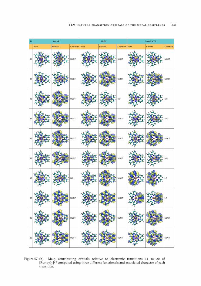
11.9 natural transition orbitals of the metal complexes 231
/
N B3LYP PBE0 CAM-B3LYP
Hole Particle Character Hole Particle Character Hole Particle Character
11 MLCT MLCT MLCT
12 MLCT MLCT MLCT
13 MLCT MC MC
14 MLCT MLCT MC
15 MLCT MLCT MLCT
16 MLCT MLCT MC
17 MC MLCT LC
18 MLCT MLCT LC
19 MLCT MLCT MLCT
20 MLCT MLCT MLCT
Figure 57: (b) Main contributing orbitals relative to electronic transitions 11 to 20 of[Ru(tpy)2]2+computed using three different functionals and associated character of eachtransition.
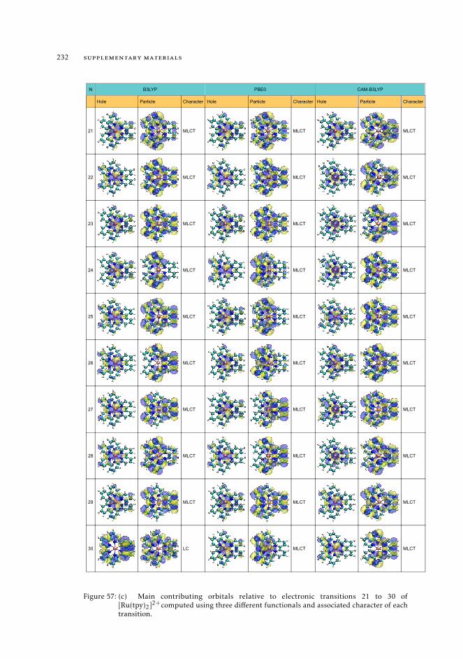
232 supplementary materials
N B3LYP PBE0 CAM-B3LYP
Hole Particle Character Hole Particle Character Hole Particle Character
21 MLCT MLCT MLCT
22 MLCT MLCT MLCT
23 MLCT MLCT MLCT
24 MLCT MLCT MLCT
25 MLCT MLCT MLCT
26 MLCT MLCT MLCT
27 MLCT MLCT MLCT
28 MLCT MLCT MLCT
29 MLCT MLCT MLCT
30 LC MLCT MLCT
Figure 57: (c) Main contributing orbitals relative to electronic transitions 21 to 30 of[Ru(tpy)2]2+computed using three different functionals and associated character of eachtransition.
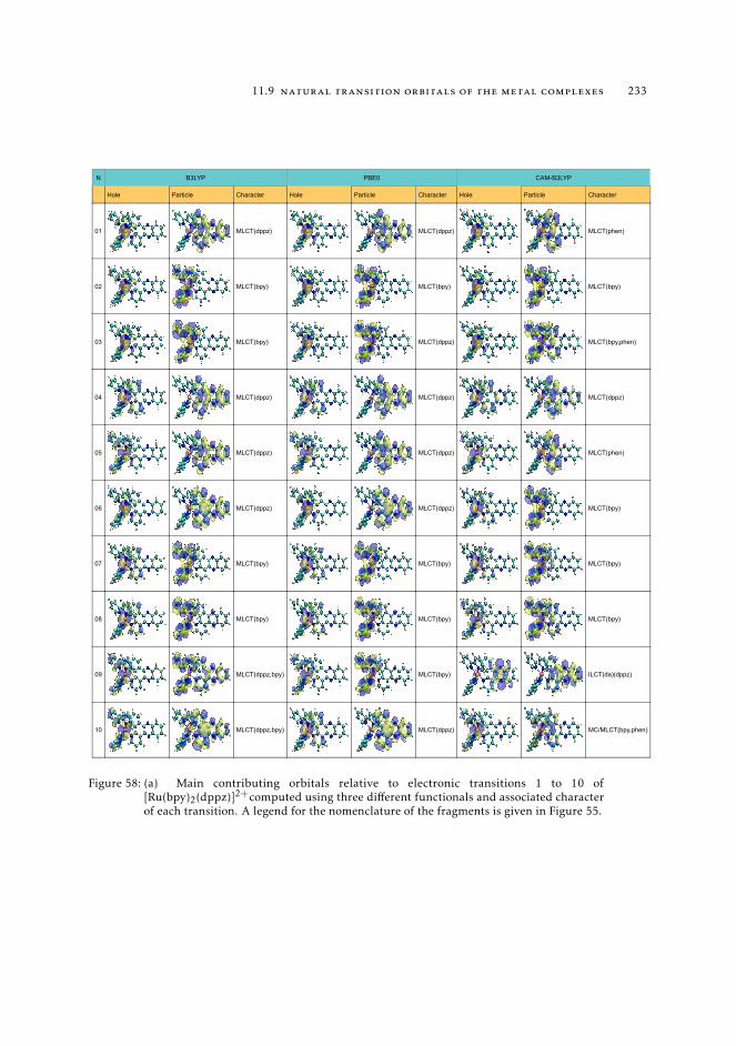
11.9 natural transition orbitals of the metal complexes 233
N B3LYP PBE0 CAM-B3LYP
Hole Particle Character Hole Particle Character Hole Particle Character
01 MLCT(dppz) MLCT(dppz) MLCT(phen)
02 MLCT(bpy) MLCT(bpy) MLCT(bpy)
03 MLCT(bpy) MLCT(dppz) MLCT(bpy,phen)
04 MLCT(dppz) MLCT(dppz) MLCT(dppz)
05 MLCT(dppz) MLCT(dppz) MLCT(phen)
06 MLCT(dppz) MLCT(dppz) MLCT(bpy)
07 MLCT(bpy) MLCT(bpy) MLCT(bpy)
08 MLCT(bpy) MLCT(bpy) MLCT(bpy)
09 MLCT(dppz,bpy) MLCT(bpy) ILCT(da)(dppz)
10 MLCT(dppz,bpy) MLCT(dppz) MC/MLCT(bpy,phen)
Figure 58: (a) Main contributing orbitals relative to electronic transitions 1 to 10 of[Ru(bpy)2(dppz)]2+computed using three different functionals and associated characterof each transition. A legend for the nomenclature of the fragments is given in Figure 55.

234 supplementary materials
N B3LYP PBE0 CAM-B3LYP
Hole Particle Character Hole Particle Character Hole Particle Character
11 MLCT(dppz) MLCT(dppz) MC/MLCT(bpy)
12 MLCT(dppz) MLCT(dppz) MC
13 MLCT(dppz) ILCT(da)(dppz) MLCT(bpy)
14 ILCT(da)(dppz) LC(dppz) LC(dppz)
15 LC(dppz) MLCT(dppz) LC(dppz)
16 MLCT(dppz) MLCT(dppz) MLCT(dppz)
17 MLCT(dppz) MLCT(dppz) MLCT(dppz)
18 MLCT(bpy) MLCT(MC) MLCT(dppz)
19 LC(dppz) MLCT(MC) MLCT(Tat)
20 MLCT(bpy) LC(dppz) MLCT(Tat)
Figure 58: b) Main contributing orbitals relative to electronic transitions 11 to 20 of[Ru(bpy)2(dppz)]2+computed using three different functionals and associated characterof each transition. A legend for the nomenclature of the fragments is given in Figure 55.

11.9 natural transition orbitals of the metal complexes 235
N B3LYP PBE0 CAM-B3LYP
Hole Particle Character Hole Particle Character Hole Particle Character
21 MC MC MC
22 ILCT(Tat)(dppz) MLCT(bpy) MLCT(dppz)
23 MC/MLCT(bpy) ILCT(dppz)(phen) MLCT(dppz)
24 MLCT(bpy) MLCT(bpy) MC
25 MLCT(bpy) MLCT(bpy) LC(bpy)
26 MLCT(bpy) MLCT(bpy) LC(bpy)
27 MLCT(bpy) MLCT(bpy) ILCT(dppz,phen)
28 MLCT(bpy) MLCT(bpy) LC(dppz)
29 LLCT(dppz)(bpy) MLCT(bpy) MLCT(bpy)
30 MC/MLCT(bpy) MLCT(bpy) MLCT(bpy)
Figure 58: c) Main contributing orbitals relative to electronic transitions 21 to 30 of[Ru(bpy)2(dppz)]2+computed using three different functionals and associated characterof each transition. A legend for the nomenclature of the fragments is given in Figure 55.
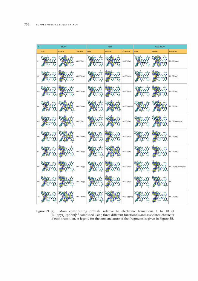
236 supplementary materials
N B3LYP PBE0 CAM-B3LYP
Hole Particle Character Hole Particle Character Hole Particle Character
01 MLCT(Tat) MLCT(Tat) MLCT(phen)
02 MLCT(bpy) MLCT(bpy) MLCT(bpy)
03 MLCT(bpy) MLCT(bpy) MLCT(bpy)
04 MLCT(tpphz) MLCT(tpphz) MLCT(Tat)
05 MLCT(Tat) MLCT(Tat) MLCT(phen-prox)
06 MLCT(tpphz) MLCT(bpy) MLCT(bpy)
07 MLCT(bpy) MLCT(Tat) MLCT(bpy)
08 MLCT(bpy) MLCT(bpy) MLCT(bpy,phen-prox)
09 MLCT(bpy) MLCT(bpy) MC
10 MLCT(tpphz) MLCT(tpphz) MLCT(bpy)
Figure 59: (a) Main contributing orbitals relative to electronic transitions 1 to 10 of[Ru(bpy)2(tpphz)]2+computed using three different functionals and associated characterof each transition. A legend for the nomenclature of the fragments is given in Figure 55.
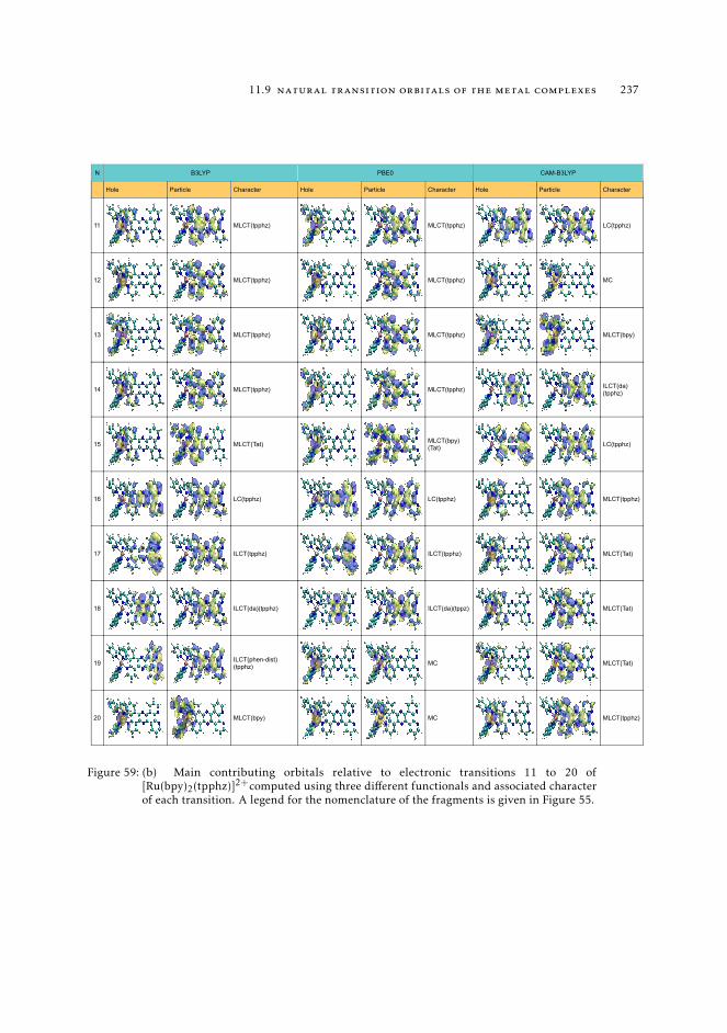
11.9 natural transition orbitals of the metal complexes 237
N B3LYP PBE0 CAM-B3LYP
Hole Particle Character Hole Particle Character Hole Particle Character
11 MLCT(tpphz) MLCT(tpphz) LC(tpphz)
12 MLCT(tpphz) MLCT(tpphz) MC
13 MLCT(tpphz) MLCT(tpphz) MLCT(bpy)
14 MLCT(tpphz) MLCT(tpphz) ILCT(da)(tpphz)
15 MLCT(Tat) MLCT(bpy)(Tat) LC(tpphz)
16 LC(tpphz) LC(tpphz) MLCT(tpphz)
17 ILCT(tpphz) ILCT(tpphz) MLCT(Tat)
18 ILCT(da)(tpphz) ILCT(da)(tppz) MLCT(Tat)
19 ILCT(phen-dist)(tpphz) MC MLCT(Tat)
20 MLCT(bpy) MC MLCT(tpphz)
Figure 59: (b) Main contributing orbitals relative to electronic transitions 11 to 20 of[Ru(bpy)2(tpphz)]2+computed using three different functionals and associated characterof each transition. A legend for the nomenclature of the fragments is given in Figure 55.
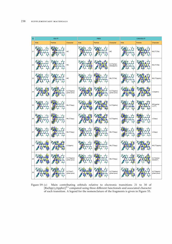
238 supplementary materials
N B3LYP PBE0 CAM-B3LYP
Hole Particle Character Hole Particle Character Hole Particle Character
21 MC MC MLCT(Tat)
22 MC ILCT(phen-dist)(tpphz) MLCT(Tat)
23 MC MLCT(Tat) MLCT(tpphz)
24 ILCT(tpphz)(phen-prox)
ILCT(tpphz)(phen-prox) LC(tpphz)
25 MLCT(bpy) ILCT(tphhz) MC(partialLLCT)
26 MLCT(bpy) ILCT(tpphz) LC(bpy)
27 MLCT(bpy) MLCT(bpy) LC(bpy)
28 LC(tpphz) MLCT(bpy) MLCT(tpphz)
29 ILCT(tpphz)(phen-prox) MLCT(bpy) ILCT(phen-
dist)(taT)
30 ILCT(taT)(phen-prox)
ILCT(tphhz)(phen-prox)
ILCT(tpphz)(phen-prox)
Figure 59: (c) Main contributing orbitals relative to electronic transitions 21 to 30 of[Ru(bpy)2(tpphz)]2+computed using three different functionals and associated characterof each transition. A legend for the nomenclature of the fragments is given in Figure 55.

Part V
RÉSUMÉ EN FRANÇAIS

12RESUMÉ EN FRANÇAIS
12.1 introduction
12.1.1 L’art de construire des modèles simples pour décrire des excitations électroniquescomplexes.
Les molécules "photo-actives " sont celles dont la réponse observable peut être provoquéepar une interaction avec la lumière [14]. La perturbation de la structure électroniquepeut être libérée par une réaction chimique induite, un changement de couleur ou deluminescence, une altération des propriétés magnétiques ou une combinaison des pos-sibilités précédemment évoquées. Les molécules (et les matériaux) possédant de tellespropriétés trouvent des applications dans un large éventail de domaines différents, et ilest possible de fabriquer des dispositifs qui exploitent leurs propriétés intrinsèques à desfins particulières, du monde biologique et médical [15, 16] au stockage optoélectroniqueet énergétique [17, 18]. La recherche constante de nouvelles molécules photo-activesd’intérêt dans ces domaines est motivée par la nécessité d’une plus grande efficacité,d’une meilleure performance et de coûts réduits. L’innovation dans ce domaine ne peutqu’être liée à la connaissance précise des mécanismes a l’origine les phénomènes photo-induits, au niveau moléculaire, et encore plus profondément au niveau des structuresélectroniques. Les processus induits par la lumière peuvent être appréhendés en termesde réorganisation de la densité électronique, et la question de savoir comment la densitéélectronique se redistribue en réponse à une perturbation induite par la lumière peutêtre traitée. Il est évident que la capacité de moduler soigneusement l’ampleur d’uneperturbation induite par la lumière est cruciale pour la conception rationnelle d’une telleclasse de molécules.
La chimie théorique a maintenant atteint un niveau de spécificité et de diversificationqui permet de caractériser l’ampleur d’une déformation ou la réactivité à l’état excitéd’un chromophore donné en appliquant simplement différentes stratégies et outils infor-matiques, et il est possible d’obtenir une description complète d’un processus réactif -c’est-à-dire son évolution selon une coordonnée de réaction spécifique - de l’absorptiond’énergie à la formation des photo-produits. Avec le ressources actuellement disponibleet les développements récents dans les méthodes théoriques telles que la théorie fonc-tionnelle de la densité en fonction du temps (TDDFT), la chimie computationnelle a déjàdémontré sa capacité à fournir des solutions pour une caractérisation en profondeur deces processus et est bien placée pour mener les découvertes à travers la conception pré-synthétique rationnelle. Les nombreux travaux publiés au cours des dernières décenniessur les états excités témoignent de la pertinence de ce sujet dans la recherche actuelle.
241
242 resumé en français
Les approches possibles pour l’étude des processus photochimiques sont multiples.En général, deux grandes catégories peuvent être identifiées. La première consiste àétudier l’évolution temporelle d’un paquet d’ondes grâce à la résolution de l’équation deSchrödinger dépendante du temps. Une deuxième approche - celle que nous adoptonsdans cette thèse - consiste à séquencer le cours d’une réaction induite par la lumière parla caractérisation de minima sur les surfaces d’énergie potentielle le long desquelles laréaction se déroule, identifiant ainsi les étapes pertinentes du trajet photochimique quirelie la région Franck-Condon, où le système absorbe, au retour à l’état fondamental, avecformation des photo-produits.
En plus de l’énergie de la réaction, une quantité essentielle que l’on peut examinerpour comprendre et moduler les propriétés d’état excité desdits systèmes moléculaires,est la densité électronique. Il est bien connu que les propriétés photo-physiques d’unsystème moléculaire donné peuvent être fortement influencées et sont généralementprédéterminées par la présence de caractéristiques structurales particulières, par exemple,des groupes très fortement électroattracteurs qui dirigent le transfert de charge à l’étatexcité. Dans ce contexte, au cours des dernières années, des ressources considérables ontété consacrées à l’élaboration de stratégies efficaces pour caractériser qualitativement etquantitativement ce transfert de charge photo-induit et pour contrôler différents processusà l’état excité qui peuvent donner lieu à des caractéristiques photo-physiques potentielle-ment utiles. C’est dans ce contexte général que se positionne cette thèse. Tout au longde ce travail, nous discuterons de la façon dont les informations combinées fournies parl’énergie et la densité peuvent fournir une vision complète des processus photo-induits,dans toute leur complexité, et avec la précision souhaitée. L’énergie permet de caractériserles propriétés locales des surfaces d’énergie potentielles, par exemple, les points de selle,les points maximum et minimum, les pentes et les barrières énergétiques, les intersectionsentre les états. L’analyse des distributions électroniques de densité ajoute les nuancessouhaitées à cette description quelque peu discrète.
12.1.2 Contexte générale de la thèse
De nos jours, nous savons que la variation de densité d’électrons d’un chromophore résultede la photogénération d’un exciton, c’est-à-dire de la génération d’une paire électron-trou.De nombreux travaux peuvent être trouvés dans la littérature traitant de la définitionde méthodologies systématiques mais rentables et précises pour la description des étatsexcités verticaux [19–21]. Au cours des dernières décennies, les progrès réalisés dansce domaine ont prouvé la capacité de la TDDFT à fournir une description objective etcomplète des architectures moléculaires, du modèle aux systèmes complexes et pertinentssur le plan chimique Curutchet:2016fk,Hagfeldt:2010,Daniel:2015ew. Les approchesfondées sur la TDDFT sont largement utilisées en raison de leur rapport coût-précisionfavorable et de leur capacité à intégrer les effets sur l’environnement, d’une manière peucoûteuse sur le plan informatique. De nombreux travaux [25, 26], évaluant et examinantla performance de la TDDFT par rapport aux méthodes basées sur la fonction d’onde etles méthodes expérimentales ont contribué à mettre en évidence les lacunes des approches
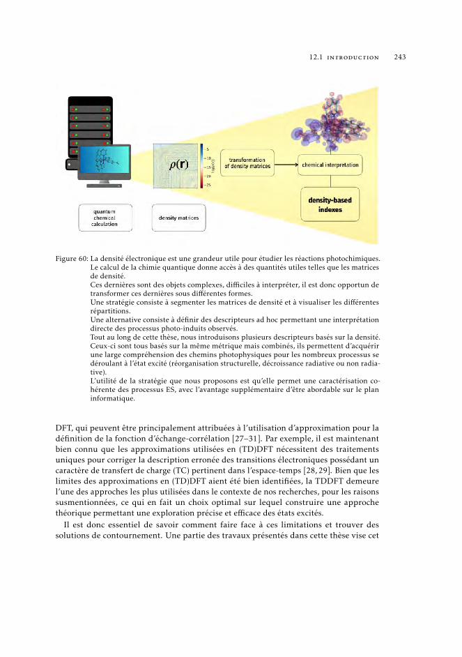
12.1 introduction 243
Figure 60: La densité électronique est une grandeur utile pour étudier les réactions photochimiques.Le calcul de la chimie quantique donne accès à des quantités utiles telles que les matricesde densité.Ces dernières sont des objets complexes, difficiles à interpréter, il est donc opportun detransformer ces dernières sous différentes formes.Une stratégie consiste à segmenter les matrices de densité et à visualiser les différentesrépartitions.Une alternative consiste à définir des descripteurs ad hoc permettant une interprétationdirecte des processus photo-induits observés.Tout au long de cette thèse, nous introduisons plusieurs descripteurs basés sur la densité.Ceux-ci sont tous basés sur la même métrique mais combinés, ils permettent d’acquérirune large compréhension des chemins photophysiques pour les nombreux processus sedéroulant à l’état excité (réorganisation structurelle, décroissance radiative ou non radia-tive).L’utilité de la stratégie que nous proposons est qu’elle permet une caractérisation co-hérente des processus ES, avec l’avantage supplémentaire d’être abordable sur le planinformatique.
DFT, qui peuvent être principalement attribuées à l’utilisation d’approximation pour ladéfinition de la fonction d’échange-corrélation [27–31]. Par exemple, il est maintenantbien connu que les approximations utilisées en (TD)DFT nécessitent des traitementsuniques pour corriger la description erronée des transitions électroniques possédant uncaractère de transfert de charge (TC) pertinent dans l’espace-temps [28, 29]. Bien que leslimites des approximations en (TD)DFT aient été bien identifiées, la TDDFT demeurel’une des approches les plus utilisées dans le contexte de nos recherches, pour les raisonssusmentionnées, ce qui en fait un choix optimal sur lequel construire une approchethéorique permettant une exploration précise et efficace des états excités.
Il est donc essentiel de savoir comment faire face à ces limitations et trouver dessolutions de contournement. Une partie des travaux présentés dans cette thèse vise cet
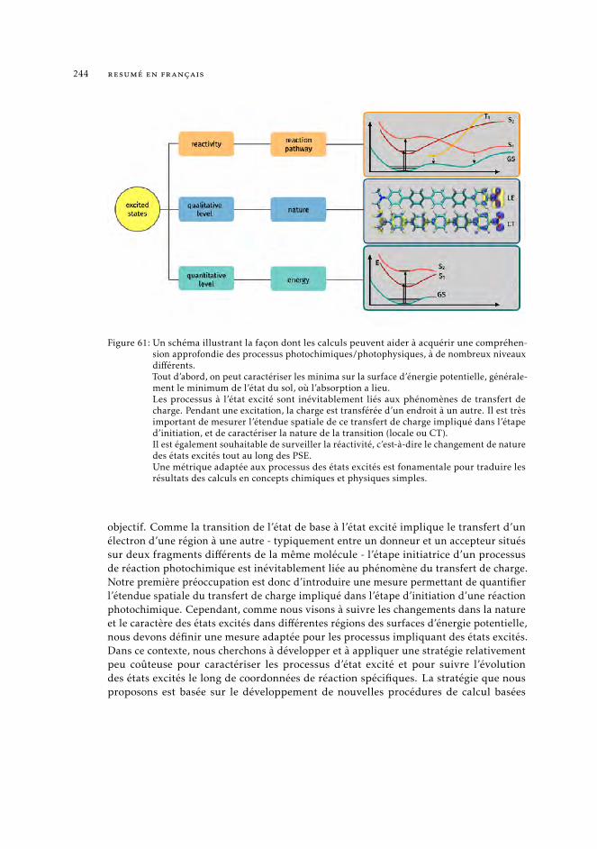
244 resumé en français
Figure 61: Un schéma illustrant la façon dont les calculs peuvent aider à acquérir une compréhen-sion approfondie des processus photochimiques/photophysiques, à de nombreux niveauxdifférents.Tout d’abord, on peut caractériser les minima sur la surface d’énergie potentielle, générale-ment le minimum de l’état du sol, où l’absorption a lieu.Les processus à l’état excité sont inévitablement liés aux phénomènes de transfert decharge. Pendant une excitation, la charge est transférée d’un endroit à un autre. Il est trèsimportant de mesurer l’étendue spatiale de ce transfert de charge impliqué dans l’étaped’initiation, et de caractériser la nature de la transition (locale ou CT).Il est également souhaitable de surveiller la réactivité, c’est-à-dire le changement de naturedes états excités tout au long des PSE.Une métrique adaptée aux processus des états excités est fonamentale pour traduire lesrésultats des calculs en concepts chimiques et physiques simples.
objectif. Comme la transition de l’état de base à l’état excité implique le transfert d’unélectron d’une région à une autre - typiquement entre un donneur et un accepteur situéssur deux fragments différents de la même molécule - l’étape initiatrice d’un processusde réaction photochimique est inévitablement liée au phénomène du transfert de charge.Notre première préoccupation est donc d’introduire une mesure permettant de quantifierl’étendue spatiale du transfert de charge impliqué dans l’étape d’initiation d’une réactionphotochimique. Cependant, comme nous visons à suivre les changements dans la natureet le caractère des états excités dans différentes régions des surfaces d’énergie potentielle,nous devons définir une mesure adaptée pour les processus impliquant des états excités.Dans ce contexte, nous cherchons à développer et à appliquer une stratégie relativementpeu coûteuse pour caractériser les processus d’état excité et pour suivre l’évolutiondes états excités le long de coordonnées de réaction spécifiques. La stratégie que nousproposons est basée sur le développement de nouvelles procédures de calcul basées
12.2 contexte théorique et méthodes 245
sur la TDDFT et sur l’utilisation de descripteurs de densité spécialement développés.Ces derniers reposent tous sur la même métrique mais, lorsqu’ils sont combinés, ilspermettent d’acquérir une image qualitative mais aussi une compréhension large desvoies photophysiques des processus multiples et simultanés qui se déroulent à l’état excité(réorganisation structurelle, désintégration non radiative). Ces types d’indices traduisentles résultats de calcul en concepts chimiques et physiques simples, fournissant ainsi uneinterprétation qualitative des phénomènes observés expérimentalement.
12.2 contexte théorique et méthodes
Ce travail s’intéresse principalement à la description théorique des processus d’excitationélectronique et à l’évolution temporelle associée des photochromes impliqués. Les méth-odes ab initio basées sur la structure électronique répondent à cette problématique enfournissant une voie d’investigation des propriétés électroniques via la résolution del’équation de Schrödinger électronique - ici non relativiste - sans l’addition d’aucunparamètre réglable. Pour un système composé d’électrons et de noyaux, cela signifie quenous voulons tout d’abord déterminer des grandeurs telles que les énergies totales del’état fondamental, les distributions électroniques de densité, les géométries d’équilibre,les longueurs et angles de liaison, les forces et constantes élastiques, les moments dipo-laires et polarisabilités statiques, les moments magnétiques. Plus généralement, toutes lesobservables qui tombent dans le domaine d’applicabilité de la théorie fonctionnelle de ladensité (DFT) de l’état fondamental [32].
Parmi les méthodologies ab initio, la DFT constitue une approche formellement exactedu problème à N corps. En outre, le DFT définit les prémices de base d’un autre cadrethéorique et computationnel, la théorie de la fonctionnelle de la densité dépendante dutemps (TDDFT) [32]. La TDDFT permet de décrire le comportement des systèmes quan-tiques hors de leur équilibre et s’applique donc à la description des processus d’excitationélectronique qui sont décrits par l’équation de Schrödinger électronique (non relativiste)dépendante du temps. Bien que le concept de "hors d’équilibre" puisse délimiter toute unesérie de scénarios différents, l’image qui nous intéresse plus particulièrement concerne lessystèmes qui sont initialement dans leur état fondamental et qui sont perturbés par unstimulus externe, généralement un rayonnement lumineux.
Ce phénomène est étroitement lié à diverses techniques spectroscopiques. En général,l’exécution d’une mesure spectroscopique signifie que le système en question est soumisà un certain stimulus externe - c’est-à-dire un champ électromagnétique - qui induit unchangement dans l’échantillon, comme des transitions électroniques. Les effets de cetteaction sont ensuite mesurés et analysés par un détecteur, révélant les propriétés spectralesassociées du système à l’étude. Il existe de nombreuses techniques spectroscopiquesdifférentes. Dans ce travail, nous traiterons principalement la description des processusd’absorption et d’émission, qui sont généralement étudiés par spectroscopie d’absorptionet de fluorescence UV-visible. Les deux techniques appartiennent à la classe des spectro-scopies linéaires, ce qui signifie que le changement qu’elles mesurent est linéairementproportionnel à la force de la perturbation appliquée. Toutefois, il convient de mentionner
246 resumé en français
que les spectroscopies non linéaires peuvent également être étudiées par TDDFT. Dansle chapitre 2 du manuscript, nous passons d’abord en revue les bases de la DFT à l’étatfondamental, puis nous explorons son extension aux états excités, en utilisant le cadre dela TDDFT. De plus, nous présentons un certain nombre de concepts et d’approximationsutiles liés à l’étude des processus photochimiques.
12.3 méthodes de description des excitations électroniques : une vue
d’ensemble
Dans le chapitre 2, nous avons présenté une description générale des processus pho-tochimiques. Le chapitre 3, donne un aperçu des outils existants qui ont été développéspour analyser ces processus d’un point de vue théorique. En particulier, ces méthodesvisent à quantifier la redistribution de la densité de charge impliquée dans l’excitation etpermettent une description concise de la transition électronique.
Le but de ce chapitre est de donner un aperçu des méthodologies qui ont été conçues aucours des dernières décennies pour étudier la localisation des états excités, en soulignantles qualités et la nouveauté de chacun. Parmi les premières analyses détaillées des étatsexcités figurent les contributions de Luzanov [93, 96–102], qui a d’abord introduit des"concepts explicites et des critères définis" impliquant l’estimation de la localisationdes états excités et le transfert de charge pour interpréter les transitions électroniques.En particulier, il a d’abord suggéré de rejeter l’analyse orbitale en faveur de certainesentités non invariantes dérivées des matrices de densité de transition [96]. Les grandeursessentielles de cette analyse, qu’il résumera plus tard sous le nom d’analyse structurale àl’état excité (ESSA) [102], sont les indices de localisation d’excitation pour l’évaluationquantitative du transfert de charge total entre fragments. Cette métrique de transfertde charge est basée sur la projection de la fonction de l’onde d’excitation dans la baseatomique spin-orbitale et mesure la probabilité de transfert d’un électron d’un fragmentmoléculaire à un autre.
Une position pertinente dans cette aperçu des indices basés sur la densité est due àla métrique de transfert de charge (DCT) [1], qui constitue le fondement théorique del’analyse de l’état excité réalisée dans ce travail. La métrique DCT réside dans la partitiondu 1DDM et dans la définition correspondante des distributions de charges positiveset négatives associées à la transition électronique. En s’appuyant sur une répartitionsimilaire du 1DDM, Etienne [103–106] a dérivé plusieurs descripteurs additionnels etperspicaces dédiés à l’étude de la topologie des états excités basés sur les centroïdes decharge obtenus à partir des matrices de densité Attachment/Detachment (initialementprésentées pour l’analyse des états excités par Head-Gordon [91]). Bien que cette approcheconsiste également en une analyse vectorielle de la distribution des différences de densitéinduites par la transition, il existe des différences substantielles par rapport à la métriqueDCT, que nous illustrerons plus en détail plus loin dans cette discussion. De plus, lemême auteur a largement contribué à former un formalisme cohérent et général pourl’analyse topologique des transitions électroniques à partir de calculs d’états excités àréférence unique, faisant le pont entre l’approche 1DDM et l’approche 1TDM [94].
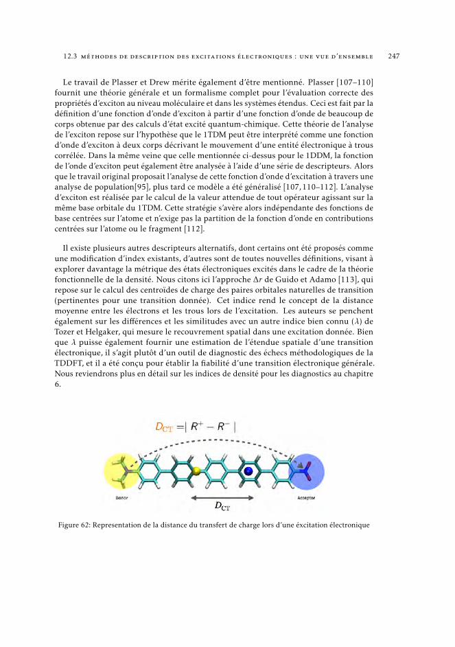
12.3 méthodes de description des excitations électroniques : une vue d’ensemble 247
Le travail de Plasser et Drew mérite également d’être mentionné. Plasser [107–110]fournit une théorie générale et un formalisme complet pour l’évaluation correcte despropriétés d’exciton au niveau moléculaire et dans les systèmes étendus. Ceci est fait par ladéfinition d’une fonction d’onde d’exciton à partir d’une fonction d’onde de beaucoup decorps obtenue par des calculs d’état excité quantum-chimique. Cette théorie de l’analysede l’exciton repose sur l’hypothèse que le 1TDM peut être interprété comme une fonctiond’onde d’exciton à deux corps décrivant le mouvement d’une entité électronique à trouscorrélée. Dans la même veine que celle mentionnée ci-dessus pour le 1DDM, la fonctionde l’onde d’exciton peut également être analysée à l’aide d’une série de descripteurs. Alorsque le travail original proposait l’analyse de cette fonction d’onde d’excitation à travers uneanalyse de population[95], plus tard ce modèle a été généralisé [107, 110–112]. L’analysed’exciton est réalisée par le calcul de la valeur attendue de tout opérateur agissant sur lamême base orbitale du 1TDM. Cette stratégie s’avère alors indépendante des fonctions debase centrées sur l’atome et n’exige pas la partition de la fonction d’onde en contributionscentrées sur l’atome ou le fragment [112].
Il existe plusieurs autres descripteurs alternatifs, dont certains ont été proposés commeune modification d’index existants, d’autres sont de toutes nouvelles définitions, visant àexplorer davantage la métrique des états électroniques excités dans le cadre de la théoriefonctionnelle de la densité. Nous citons ici l’approche ∆r de Guido et Adamo [113], quirepose sur le calcul des centroïdes de charge des paires orbitales naturelles de transition(pertinentes pour une transition donnée). Cet indice rend le concept de la distancemoyenne entre les électrons et les trous lors de l’excitation. Les auteurs se penchentégalement sur les différences et les similitudes avec un autre indice bien connu (λ) deTozer et Helgaker, qui mesure le recouvrement spatial dans une excitation donnée. Bienque λ puisse également fournir une estimation de l’étendue spatiale d’une transitionélectronique, il s’agit plutôt d’un outil de diagnostic des échecs méthodologiques de laTDDFT, et il a été conçu pour établir la fiabilité d’une transition électronique générale.Nous reviendrons plus en détail sur les indices de densité pour les diagnostics au chapitre6.
Figure 62: Representation de la distance du transfert de charge lors d’une éxcitation électronique
248 resumé en français
Une autre stratégie consiste à caractériser quantitativement le déplacement de chargeoccourant lors de l’excitation en intégrant la densité électronique selon un axe choisi(qui coïncide avec la coordonnée de transfert d’électrons) [114]. Dans l’ensemble, cesétudes ont contribué à l’évolution des modèles utilisés pour l’étude des états excités. Nousdonnons ci-dessous une description plus détaillée de certains des descripteurs mentionnésci-dessus. Ce résumé vise à donner une vue d’ensemble des méthodologies disponiblespour l’examen des excitations électroniques et à fournir un contexte pour les travauxprésentés plus loin.
12.4 une mesure de transfert de charge dans les transictions électron-
iques
L’approche de la théorie de la réponse dépendant du temps décrite au chapitre 4 fournitune voie pour accéder aux énergies d’excitation et aux moments de transition. Lesénergies totales de l’état excité (ES) sont alors accessibles en ajoutant l’énergie d’excitationà l’énergie correspondante de l’état fondamental (GS). Cette méthodologie donne accèsà des objets utiles, tels que la matrice de différence de densité (1DDM), qui contiennentles informations relatives à la polarisation du nuage électronique se produisant dansl’excitation. Dans le cadre de la théorie de la fonctionnelle de la densité dépendante dutemps (TDDFT), en outre, pour améliorer la description des matrices de densité, on peutaussi réaliser un traitement post linéaire aux calcul de l’état excité, par l’application dela méthode nommée "Z-Vector" [126]. Dans le schéma TDDFT, ce computation résulteen l’ajout d’une matrice (termes virtuels occupés) a la 1DDM pour tenir compte del’assouplissement de la densité après la génération de trous/particules. La densité del’état excité redistribuée qui en résulte est ce qu’on appelle la matrice de densité rélaxée.
Cette procédure soulève la question de savoir comment la qualité des densités calculéesaffecte les descripteurs qui en sont directement dérivés. Cette question fait l’objet d’unede nos publications récentes: "Comment les descripteurs de transfert de charge sont-ilsaffectés par la qualité de la densité électronique sous-jacente ? par Marco Campetella,Michael J. Frisch, Giovanni Scalmani, Carlo Adamo, Ilaria Ciofini et moi-même, publiésdans le Journal of Computational Chemistry. Le chapitre 4 de ce manuscrit constitue uneadaptation de cette publication.
Dans le but d’étudier qualitativement et quantitativement l’impact de l’utilisation de ladensité relaxée ou non relaxée pour l’estimation de la nature et des caractéristiques desétats excités électroniques, nous avons analysé le l’effet de l’utilisation de 52 fonctionnellesde corrélation des échanges différents pour la prédiction de la distance de transfert decharge DCT [1] pour une famille prototype composants de type push-pull.
Nos résultats montrent que bien qu’une évaluation qualitativement cohérente de lanature des états excités soit obtenue en utilisant la densité non relaxée ou relaxée, d’unpoint de vue quantitatif, nous observons de grandes différences dans la distance detransfert de charge pour les transitions électroniques ayant un caractère CT important. Cecomportement est indépendant de la nature de la fonction d’échange-corrélation utilisée.
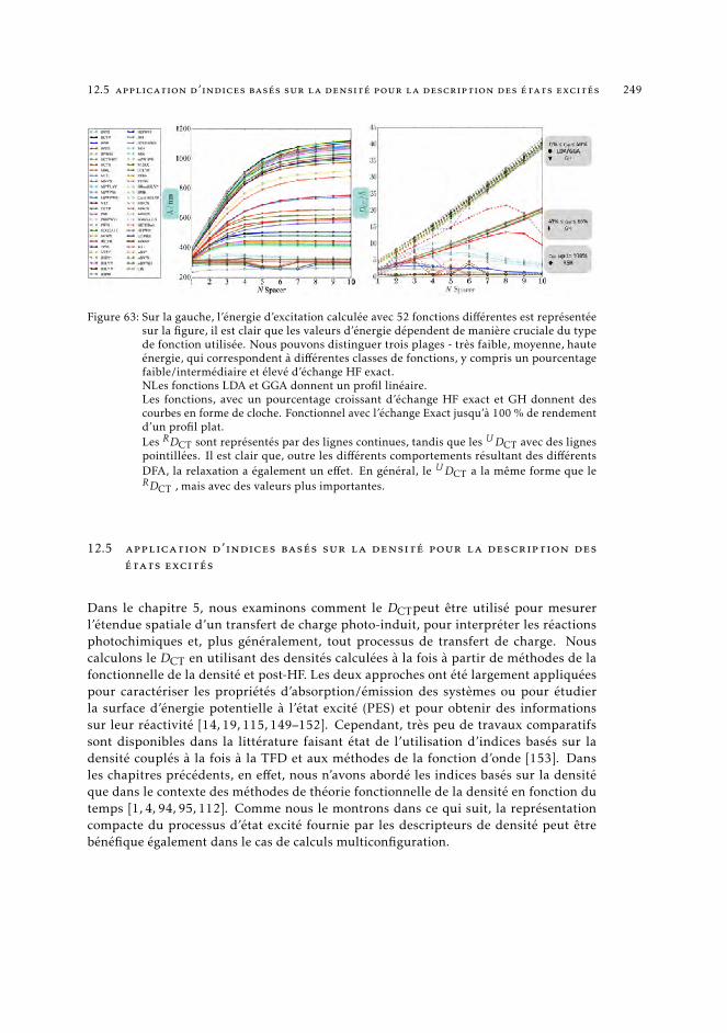
12.5 application d’indices basés sur la densité pour la description des états excités 249
Figure 63: Sur la gauche, l’énergie d’excitation calculée avec 52 fonctions différentes est représentéesur la figure, il est clair que les valeurs d’énergie dépendent de manière cruciale du typede fonction utilisée. Nous pouvons distinguer trois plages - très faible, moyenne, hauteénergie, qui correspondent à différentes classes de fonctions, y compris un pourcentagefaible/intermédiaire et élevé d’échange HF exact.NLes fonctions LDA et GGA donnent un profil linéaire.Les fonctions, avec un pourcentage croissant d’échange HF exact et GH donnent descourbes en forme de cloche. Fonctionnel avec l’échange Exact jusqu’à 100 % de rendementd’un profil plat.Les RDCT sont représentés par des lignes continues, tandis que les UDCT avec des lignespointillées. Il est clair que, outre les différents comportements résultant des différentsDFA, la relaxation a également un effet. En général, le UDCT a la même forme que leRDCT , mais avec des valeurs plus importantes.
12.5 application d’indices basés sur la densité pour la description des
états excités
Dans le chapitre 5, nous examinons comment le DCTpeut être utilisé pour mesurerl’étendue spatiale d’un transfert de charge photo-induit, pour interpréter les réactionsphotochimiques et, plus généralement, tout processus de transfert de charge. Nouscalculons le DCT en utilisant des densités calculées à la fois à partir de méthodes de lafonctionnelle de la densité et post-HF. Les deux approches ont été largement appliquéespour caractériser les propriétés d’absorption/émission des systèmes ou pour étudierla surface d’énergie potentielle à l’état excité (PES) et pour obtenir des informationssur leur réactivité [14, 19, 115, 149–152]. Cependant, très peu de travaux comparatifssont disponibles dans la littérature faisant état de l’utilisation d’indices basés sur ladensité couplés à la fois à la TFD et aux méthodes de la fonction d’onde [153]. Dansles chapitres précédents, en effet, nous n’avons abordé les indices basés sur la densitéque dans le contexte des méthodes de théorie fonctionnelle de la densité en fonction dutemps [1, 4, 94, 95, 112]. Comme nous le montrons dans ce qui suit, la représentationcompacte du processus d’état excité fournie par les descripteurs de densité peut êtrebénéfique également dans le cas de calculs multiconfiguration.
250 resumé en français
Dans ce qui suit, nous considérons le cas d’une simple réaction de transfert de protonsà l’état excité intramoléculaire. Nous montrons l’application des index de la densité(DCT) en utilisant à la fois fonctions d’ondes calculé par methodes du champ multi-configurationnel auto-cohérent (CASSCF-CASPT2) et derivé de méthodes de la fonc-tionnelle de la densité. Les résultats confirment que, même dans le cas de méthodesmulticonfigurationnelles, la DCT fournit des informations utiles concernant à la fois lacharge et la réorganisation structurelle d’une molécule à l’état excité. Ce sujet fait l’objetd’une de nos récentes publications : "Using Density-Based Indexes and Wave FunctionMethods for the Description of Excited States : Excited State Proton-Transfer Reactions asa Test Case", publié par moi-même, Juan Sanz Garcia, Marco Campetella et Ilaria Ciofinidans le Journal of Physical Chemistry A. Le présent chapitre constitue une adaptation decette dernière publication.
12.6 la description problématique des excitations de transfert de charges
à l’aide de la dft
Lorsque la TDDFT est utilisée, les états de transfert de charge (TC) a longue distancecorrespondent à des états excités dont le recouvrement entre les distributions des trousphoto-excités et des charges électroniques est négligeable. Ce résultat, cependant, esttypiquement un artefact de la méthode résultant de l’utilisation de potentiels xc ap-prochés, dont les potentiels ont un tracé asymptotique incorrecte et sont erronémentcontinus. Le potentiel exact d’échange-corrélation d’un état de transfert de charge sautede façon discontinue d’un montant de ∆xc lorsque le nombre d’électrons croise l’entier.En conséquence, les énergies d’excitation de ces états sont généralement largement sous-estimées au point qu’elles peuvent apparaître énergie inférieure aux états optiques. Dansle chapitre 6, nous discutons d’une méthodologie permettant de repérer ces états nonphysiques erronés, grâce à un nouvel indice peu coûteux en termes de calcul - MAC.
La formulation de l’indice MACest dérivée d’une modification de la relation de Mullikende l’énergie de transition pour les excitations de TC.Elle repose sur deux ingrédients debase : une distance effective de CT, calculée à l’aide de notre indice basé sur la densité(DCT), et une estimation pondérée du potentiel d’ionisation et de l’affinité des électrons.Pour vérifier la robustesse de notre approche, nous avons testé notre indice sur certainssystèmes modèles, représentatifs des excitations de TC intermoléculaires et intramolécu-laires, en utilisant des fonctionnelles appartenant à différentes classes (approximationde gradient généralisée, hybrides globaux et hybrides séparés en gamme). Ces résultatspréliminaires confirment que les états fantômes sont correctement repérés, même dans lecas délicat d’excitations intramoléculaires présentant une délocalisation importante entredonneurs et accepteurs, régime dans lequel la formulation standard de Mulliken atteintses limites. La première partie de cet chapitre est adaptée d’une publication précédentede moi-même, Marco Campetella, Mike J. Frisch, Giovanni Scalmani, Ilaria Ciofini etCarlo Adamo [5].
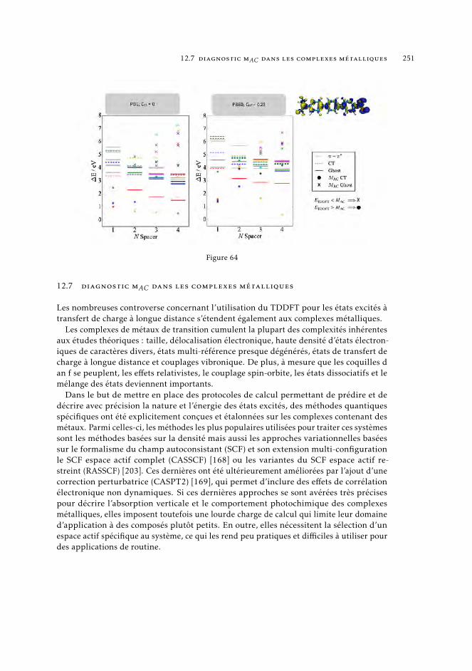
12.7 diagnostic mAC dans les complexes métalliques 251
Figure 64
12.7 diagnostic mAC dans les complexes métalliques
Les nombreuses controverse concernant l’utilisation du TDDFT pour les états excités àtransfert de charge à longue distance s’étendent également aux complexes métalliques.
Les complexes de métaux de transition cumulent la plupart des complexités inhérentesaux études théoriques : taille, délocalisation électronique, haute densité d’états électron-iques de caractères divers, états multi-référence presque dégénérés, états de transfert decharge à longue distance et couplages vibronique. De plus, à mesure que les coquilles dan f se peuplent, les effets relativistes, le couplage spin-orbite, les états dissociatifs et lemélange des états deviennent importants.
Dans le but de mettre en place des protocoles de calcul permettant de prédire et dedécrire avec précision la nature et l’énergie des états excités, des méthodes quantiquesspécifiques ont été explicitement conçues et étalonnées sur les complexes contenant desmétaux. Parmi celles-ci, les méthodes les plus populaires utilisées pour traiter ces systèmessont les méthodes basées sur la densité mais aussi les approches variationnelles baséessur le formalisme du champ autoconsistant (SCF) et son extension multi-configurationle SCF espace actif complet (CASSCF) [168] ou les variantes du SCF espace actif re-streint (RASSCF) [203]. Ces dernières ont été ultérieurement améliorées par l’ajout d’unecorrection perturbatrice (CASPT2) [169], qui permet d’inclure des effets de corrélationélectronique non dynamiques. Si ces dernières approches se sont avérées très précisespour décrire l’absorption verticale et le comportement photochimique des complexesmétalliques, elles imposent toutefois une lourde charge de calcul qui limite leur domained’application à des composés plutôt petits. En outre, elles nécessitent la sélection d’unespace actif spécifique au système, ce qui les rend peu pratiques et difficiles à utiliser pourdes applications de routine.
252 resumé en français
Des méthodes hybrides ont également fait leur apparition [204], qui combinent la DFTà courte distance et la fonction d’onde ou les approches perturbatrices à longue distance.Ces dernières présentent toutefois les mêmes inconvénients.
Les approches TDDFT, au contraire, ont l’avantage d’une échelle favorable, qui adéterminé leur large diffusion dans le traitement des complexes à base de métaux. Enoutre, les approches fondées sur la densité limitent la dépendance de l’utilisateur au choixde la fonction de corrélation d’échange à utiliser, ce qui, en pratique, rend ces méthodespeu compliquées, bien qu’elles soient d’une précision impressionnante dans la descriptiondes propriétés structurelles et spectroscopiques des complexes de métaux de transition,du moins en ce qui concerne l’état électronique de base et les états excités les plus bas.Il n’est pas surprenant que les calculs de TDDFT et les spectres simulés obtenus à partirde ceux-ci soient de plus en plus utilisés pour étayer les résultats expérimentaux, où lacaractérisation réelle de la nature de la transition observée par des calculs de structureélectronique peut apporter un complément et un renforcement extrêmement précieuxaux études expérimentales [24, 205, 206].
Pour ces études comparatives, le choix de la fonction de corrélation et d’échange estgénéralement basé sur des travaux préalables traitant de composés similaires, montrantun bon accord avec les résultats expérimentaux. Cependant, la correspondance entre lesspectres expérimentaux et théoriques peut simplement survenir en raison d’une heureusecompensation des erreurs. Les limites de la DFT et de la TDDFT s’appliquent en effet égale-ment aux complexes contenant des métaux. Une fausse tracé asymptotique typique desfonctionnelles d’échange local a de fâcheuses conséquences sur les énergies d’excitationcalculées de cette classe de composés, qui à leur tour, peuvent fortement affecter lespropriétés photo-physiques et photochimiques prévues, et avec elles, l’interprétation dumécanisme des processus d’état excité correspondants. Une note de prudence est doncnécessaire. En particulier, les complexes de métaux de transition sont souvent conçus dansle but précis d’améliorer le caractère de la CT dans l’état électronique de base, ou dansl’état excité le plus bas, pour obtenir des composés possédant simultanément une faiblelongueur d’onde d’absorption et un coefficient d’extinction molaire élevé. Par exemple,les composés possédant de telles propriétés font l’objet de recherches approfondies dansle cadre de la thérapie photodynamique (TPD) [11, 207], des complexes de récolte de lalumière dans les plantes et les bactéries [22], ainsi que pour les applications des cellulessolaires sensibilisées aux colorants [205]. Les états TC sont ensuite générés en fonction-nalisant les structures des complexes métalliques avec les groupes donneurs/accepteursappropriés.
Naturellement, la description de ces transitions dans l’espace dépend fortement del’approximation fonctionnelle de la densité choisie. Les complexes de métaux de transitionprésentant de telles caractéristiques sont en principe susceptibles de présenter des étatsde transfert de charge fantôme et ligand-à-ligand, en particulier dans le cas de systèmesavec des ligands étendus. Ces derniers, au contraire, sont généralement bien décrits carle degré de recouvrement entre les orbitales du métal d et l’orbitale d’acceptation surle ligand est important. Il s’ensuit que pour caractériser ces composés avec la précisionsouhaitée, il est nécessaire d’utiliser la méthodologie appropriée et d’adopter une stratégie
12.8 suivi des états excités dans les systèmes moléculaires 253
adéquate pour diagnostiquer la fiabilité de l’approche TDDFT choisie. Comme nousdemontrons dans le chapitre 7, l’indice Mac peut fournir des informations pertinentespour détecter les états non physiques, qui sont calculés avec une précision insuffisante etapparaissent donc trop bas dans le spectre.
12.8 suivi des états excités dans les systèmes moléculaires
Dans les chapitres précédents, nous avons longuement discuté du concept de transfertde charges, de la manière de mesurer l’étendue spatiale d’une transition donnée, desdéfis que pose une telle mesure et de la manière de les relever. Nous avons maintenantappliqué ces concepts dans le contexte des transitions verticales, qui se produisent entrel’état de base et tout état d’intérêt excité. L’étape logique consiste à étudier le processus deréorganisation de la charge qui en découle et qui conduit à la population de l’état émissif.Cette observation est cohérente avec l’image intuitive selon laquelle, après une excitationverticale, un système aura tendance à se détendre structurellement afin de minimiser laséparation et la réorganisation de la charge de l’état excité produit. Nous étendons iciles concepts introduits précédemment pour tenir compte des transitions d’état excité àétat excité. Dans ce contexte, le DCTn’est plus strictement lié à l’amplitude spatiale de laséparation de charge produite par l’excitation électronique d’état excité à état excité, maisà la distance entre deux états excités.
Le chapitre 8 s’inscrit dans ce contexte général. L’approche que nous exposons icicombine plusieurs descripteurs de densité, conçus à l’origine pour l’interprétation quali-tative des phénomènes observés expérimentalement, et vise à fournir une image physiquesimple du mécanisme des processus d’état excité. Notre stratégie vise à permettre unecaractérisation peu coûteuse des surfaces d’énergie potentielles à l’état excité, qui peuventêtre calculées - à la volée - pour permettre à la fois l’identification des zones critiques pourles approches TDDFT et la reconnaissance qualitative - en conjonction avec des critèresénergétiques - des chemins de réaction possibles.
Nous introduisons, dans ce qui suit, un nouvel indice basé sur la densité, Π, qui peutêtre utilisé pour obtenir une mesure qualitative du travail nécessaire pour redistribuer ladensité d’électrons passant d’un état excité à un autre à une configuration électroniquedonnée. Auparavant appliqué pour révéler les canaux de désintégration non radiativedu premier état excité à l’état de base [2], ce descripteur est simple, peu coûteux, etpeut être couplé à toute méthode quantique capable de fournir une description desétats excités électroniques. En effet, il repose uniquement sur la connaissance des den-sités énergétiques et électroniques des différents états électroniques impliqués dans unedécroissance. Pour illustrer les connaissances que ces indices peuvent apporter à la de-scription des processus d’états excités, nous examinons deux types distincts de réactions.Le premier est un transfert intramoléculaire de protons se produisant dans le CPDNO(1-(cyclopropyl)diazo-2-naphtol), un composé aromatique azoïque, suivi par les processusde transfert de charge photo-induit dans le DMABN (N,N-diméthylaminobenzonitrile)et le Phen-PENMe2 (5-(4-diméthylaminophényléthylyn)-1,10-phénanthroline). Toutesces molécules sont précédemment présentées dans le Chapitre 5, où nous vérifions la
254 resumé en français
fiabilité de la méthodologie TDDFT appliquée pour calculer leurs courbes d’énergie po-tentielle le long de coordonnées de réaction spécifiques. En outre, ces systèmes ont étélargement étudiés et de nombreuses études existent dans la littérature, tant au niveauthéorique [163, 216, 217] qu’expérimental [188, 193, 218]. L’accord avec ces études an-térieures corrobore nos résultats.
Dans l’ensemble, l’indice Π s’est avéré capable d’identifier les régions où les étatsexcités sont les plus susceptibles de s’echanger. Ce chapitre constitue une adaptation dedeux travaux antérieurs de ma part, le premier publié dans le Journal of ComputationalChemistry, en collaboration avec Juan Sanz-Garcia, Marco Campetella et Ilaria Ciofini [6],le second, présenté avec Anna Perfetto et Ilaria Ciofini et publié dans le Journal ofPhotochemistry and Photobiology A.
12.9 determiner la distribution rélative des états excités le long d’un
chemin réactionnel
Le suivi de chaque état excité le long d’une coordonnée de réaction est un problèmecrucial en photochimie. Si le calcul des propriétés optiques est certainement un point dedépart, les spectres d’absorption et d’émission ne fournissent aucune information sur lechemin parcouru par chaque état excité, et il peut être compliqué d’établir le lien entrel’absorption d’énergie et la formation de photoproduits. Les descripteurs topologiquespeuvent être très utiles pour caractériser la nature d’un état excité. En particulier, ilstraduisent de manière pratique les informations contenues dans les objets mathématiques,tels que la 1DDM [115], en une représentation plus compacte et plus lisible de la transitionélectronique, et peuvent donc être utiles pour examiner la nature d’un état excité le longd’une coordonnée de réaction. Néanmoins, comprendre pleinement où, parmi toutesles positions verticales, se trouve un état d’intérêt, et cartographier la position d’un étatexcité particulier en des points successifs d’une coordonnée de réaction, reste une tâchenon triviale qui est néanmoins indispensable pour assembler une description cohérented’un chemin de réaction [151]. Ce problème constitue le nucleus du chapitre 9. Nousproposons ici une nouvelle métrique rigoureuse pour suivre les états excités le long d’unecoordonnée de réaction, basée sur le descripteur basé sur la densité DCT. Le DCT traduitles informations contenues dans les densités des états initiaux et finaux en une longueur etfournit une mesure simple de l’étendue spatiale d’une transition électronique. Nous avonsutilisé cette approche à plusieurs reprises dans les chapitres précédents, où nous avonscaractérisé la nature des états excités tout au long de coordonnées de réaction spécifiquespar leurs valeurs DCT - calculées par rapport à leur distribution de densité d’état de basecorrespondante à la même géométrie. Bien que la valeur DCT soit spécifique pour unetransition donnée, elle n’est pas suffisante pour caractériser un état de façon unique parmiun ensemble d’états excités verticaux. En fait, il peut y avoir plusieurs états proches ayantun caractère similaire, dont l’ambiguïté peut empêcher l’identification précise d’un étatd’intérêt le long d’une coordonnée de réaction.
Nous tentons de résoudre cette indétermination avec une nouvelle métrique, qui fournitune représentation unique de l’état excité. Au lieu de caractériser un état vertical en termes
12.9 determiner la distribution rélative des états excités le long d’un chemin réactionnel 255
de transition d’un électron à partir de l’état fondamental, nous utilisons la collectionde vecteurs calculés entre cet état et tout autre état, à la même géométrie. En d’autrestermes, nous caractérisons chaque état en cryptant ses connotations dans une "empreinte"spécifique à l’état. Ensuite, nous comparons chaque paire d’états en utilisant une distancegéométrique volontairement définie entre leurs empreintes correspondantes.
Nous avons implémenté une telle métrique dans un algorithme simple pour cartogra-phier l’évolution des états excités le long d’une coordonnée de réaction. L’algorithmedétermine la disposition relative d’un ensemble d’états verticaux en calculant la distanceentre les empreintes de chaque paire d’états à des étapes successives et en sélectionnantcelle qui minimise toutes les distances. Nous évaluons la performance de cette recherchede carte de réaction en comparant les résultats avec une représentation de référence, oùnous estimons la similarité entre toutes les paires d’états en inspectant visuellement lesorbitales principales et les descripteurs de densité pertinents. En outre, nous discutonsd’une alternative possible à la méthode des empreintes, qui consiste à évaluer la distanceentre chaque paire d’états en utilisant le recouvrement des fonctions d’onde correspon-dantes. Les résultats montrent que nous sommes capables de reconstruire les distributionset les croisements d’états excités tout au long de différentes coordonnées de réaction.
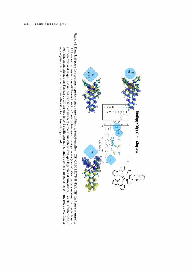
256 resumé en français
Figure
65: Dan
sla
figu
re:L
escou
leurs
représen
tent
quatre
diff
érentes
fonction
nelles
-C
IS,CA
M-B
3LYP,B
3LYP,C
IS.La
figu
rem
ontre
lesd
ifféren
cesd
ed
ensité
pou
rd
ifférents
étatsfantôm
es(p
ointsrem
plis)et
parasites
(carrés).Ces
dern
iersn
esont
que
partiellem
enterronés,c’est-à-dire
qu’ilssem
blenttrop
faiblesen
énergiem
aisleur
valeurn’est
quelégèrem
entsurestim
ée.Les
étatsfantôm
esqui
sontgravem
entaff
ectésp
arl’erreu
rde
CT
ontu
neforce
d’oscillateur
nulle,tandis
que
lesétats
parasites
ontu
neforce
d’oscillateur
nonnégligeable
etrecou
vrement
significatif
entrele
trouet
lap
articule.
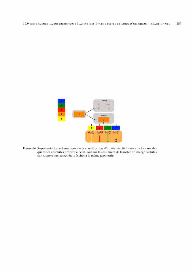
12.9 determiner la distribution rélative des états excités le long d’un chemin réactionnel 257
Figure 66: Représentation schematique de la classification d’un état éxcité basée a la fois sur desquantités absolutes propres à l’état, soit sur les distances de transfer de charge cacluléspar rapport aux autres états éxcités à la mème geometrie.

B IBL IOGRAPHY
[1] T. Le Bahers, C. Adamo, and I. Ciofini, “A Qualitative Index of Spatial Extent in Charge-Transfer Excitations.,”Journal of Chemical Theory and Computation, vol. 7, pp. 2498–2506, Aug. 2011.
[2] M. Savarese, U. Raucci, P. A. Netti, C. Adamo, N. Rega, and I. Ciofini, “A qualitative model to identifynon-radiative decay channels: the spiropyran as case study,” Theoretical Chemistry Accounts, vol. 135,pp. 211–7, Aug. 2016.
[3] J. Sanz García, F. Maschietto, M. Campetella, and I. Ciofini, “Using Density Based Indexes and Wave FunctionMethods for the Description of Excited States: Excited State Proton Transfer Reactions as a Test Case,” TheJournal of Physical Chemistry A, vol. 122, pp. 375–382, Dec. 2017.
[4] F. Maschietto, M. Campetella, M. J. Frisch, G. Scalmani, C. Adamo, and I. Ciofini, “How are the charge transferdescriptors affected by the quality of the underpinning electronic density?,” Journal of ComputationalChemistry, vol. 39, pp. 735–742, Jan. 2018.
[5] M. Campetella, F. Maschietto, M. J. Frisch, G. Scalmani, I. Ciofini, and C. Adamo, “Charge transfer excitationsin TDDFT: A ghost-hunter index,” Journal of Computational Chemistry, vol. 38, pp. 2151–2156, Sept. 2017.
[6] F. Maschietto, J. Sanz García, M. Campetella, and I. Ciofini, “Using density based indexes to characterizeexcited states evolution.,” Journal of Computational Chemistry, vol. 40, pp. 650–656, Feb. 2019.
[7] A. Perfetto, F. Maschietto, and I. Ciofini, “Following excited states in molecular systems using density-basedindexes: A dual emissive system as a test case,” "Journal of Photochemistry & Photobiology, A: Chemistry",vol. 383, p. 111978, Oct. 2019.
[8] F. Maschietto, J. S. Garcia, C. Adamo, and I. Ciofini, “Charge Transfer Metal Complexes using Time-Dependent Density Funcitional theory: hotw to spot ghost and spurious states?,” In preparation, 2019.
[9] J. Karges, F. Heinemann, F. Maschietto, M. Patra, O. Blacque, I. Ciofini, B. Spingler, and G. Gasser, “A Ru(II)polypyridyl complex bearing aldehyde functions as a versatile synthetic precursor for long-wavelengthabsorbing photodynamic therapy photosensitizers,” Bioorganic & Medicinal Chemistry, vol. 27, no. 12,pp. 2666–2675, 2019.
[10] F. Heinemann, M. Jakubaszek, J. Karges, C. Subecz, F. Maschietto, M. Dotou, J. Seguin, N. Mignet, E. V.Zahínos, M. Tharaud, O. Blacque, P. Goldner, B. Goud, B. Spingler, I. Ciofini, and G. Gasser, “TowardsDFT-Rationally Designed Long-Wavelength Absorbing Ru(II) Polypyridyl Complexes as Photosensitizers forPhotodynamic Therapy,” In preparation, 2019.
[11] J. Karges, M. Jakubaszek, F. Maschietto, J. Seguin, N. Mignet, M. Tharaud, O. Blacque, P. Goldner, B. Goud,B. Spingler, I. Ciofini, and G. Gasser, “Evaluation of the Medicinal Potential of Ruthenium(II) Polypyridinebased Complexes as One- and Two-Photon Photodynamic Therapy Photosensitizers,” In preparation, 2019.
[12] T.-T. Bui, M. Ulfa, F. Maschietto, A. Ottochian, M.-P. Nghiêm, I. Ciofini, F. Goubard, and T. Pauporté, “Designof dendritic core carbazole-based hole transporting materials for efficient and stable hybrid perovskite solarcells,” Organic Electronics, vol. 60, pp. 22–30, Sept. 2018.
[13] F. Maschietto, A. Ottochian, L. Posani, and I. Ciofini, “Mapping states along reaction coordinates: A state-specific fingerprint for efficient state tracking,” In preparation, 2019.
[14] M. Garavelli, “Computational Organic Photochemistry: Strategy, Achievements and Perspectives,”Theoretical Chemistry Accounts, vol. 116, pp. 87–105, Jan. 2006.
[15] A. Kamkaew, S. H. Lim, H. B. Lee, L. V. Kiew, L. Y. Chung, and K. Burgess, “BODIPY dyes in photodynamictherapy,” Chemical Society Reviews, vol. 42, no. 1, pp. 77–88, 2013.
[16] M. E. Alberto, N. Russo, and C. Adamo, “The contribution of computational studies to photodynamictherapy: Challenges and opportunities for the future of computational prediction,” Photodiagnosis andPhotodynamic Therapy, vol. 17, p. A52, 2017.
[17] L. Ying, C.-L. Ho, H. Wu, Y. Cao, and W.-Y. Wong, “White Polymer Light-Emitting Devices for Solid-StateLighting: Materials, Devices, and Recent Progress,” Advanced Materials, vol. 26, no. 16, pp. 2459–2473,2014.
259
260 bibliography
[18] H. Sasabe and J. Kido, “Recent Progress in Phosphorescent Organic Light-Emitting Devices,” EuropeanJournal of Organic Chemistry, vol. 2013, no. 34, pp. 7653–7663, 2013.
[19] C. Adamo, T. Le Bahers, M. Savarese, L. Wilbraham, G. García, R. Fukuda, M. Ehara, N. Rega, and I. Ciofini,“Exploring excited states using Time Dependent Density Functional Theory and density-based indexes,”Coordination Chemistry Reviews, vol. 304-305, pp. 166–178, Dec. 2015.
[20] A. Dreuw and M. Head-Gordon, “Single-reference ab initio methods for the calculation of excited states oflarge molecules,” Chemical Reviews, vol. 105, pp. 4009–4037, Nov. 2005.
[21] D. P. Chong, Recent Advances in Density Functional Methods. World Scientific, 1995.
[22] C. Curutchet and B. Mennucci, “Quantum Chemical Studies of Light Harvesting,” Chemical Reviews,vol. 117, pp. 294–343, Mar. 2016.
[23] A. Hagfeldt, G. Boschloo, L. Sun, L. Kloo, and H. Pettersson, “Dye-Sensitized Solar Cells,” Chemical Reviews,vol. 110, no. 11, pp. 6595–6663, 2010.
[24] C. Daniel, “Photochemistry and photophysics of transition metal complexes: Quantum chemistry,”Coordination Chemistry Reviews, vol. 282-283, pp. 19–32, Jan. 2015.
[25] R. Peverati and D. G. Truhlar, “Quest for a universal density functional: the accuracy of density functionalsacross a broad spectrum of databases in chemistry and physics.,” Philosophical Transactions of the RoyalSociety a-Mathematical Physical and Engineering Sciences, vol. 372, p. 20120476, Mar. 2014.
[26] Y. Zhao and D. G. Truhlar, “Density functionals with broad applicability in chemistry.,” Accounts of ChemicalResearch, vol. 41, pp. 157–167, Feb. 2008.
[27] C. A. Ullrich and Z.-h. Yang, “A Brief Compendium of Time-Dependent Density Functional Theory,”Brazilian Journal of Physics, vol. 44, pp. 154–188, Feb. 2014.
[28] L. Kronik, T. Stein, S. Refaely-Abramson, and R. Baer, “Excitation Gaps of Finite-Sized Systems fromOptimally Tuned Range-Separated Hybrid Functionals,” Journal of Chemical Theory and Computation,vol. 8, pp. 1515–1531, Apr. 2012.
[29] T. Stein, L. Kronik, and R. Baer, “Reliable prediction of charge transfer excitations in molecular complex-esusing time-dependent density functional theory,” Journal of the American Chemical Society, vol. 131,pp. 2818–2820, Mar. 2009.
[30] D. J. Tozer, “Relationship between long-range charge-transfer excitation energy error and integer discontinu-ity in Kohn-Sham theory,” Journal of Chemical Physics, vol. 119, pp. 12697–12699, Dec. 2003.
[31] S. Tretiak, K. Igumenshchev, and V. Chernyak, “Exciton sizes of conducting polymers predicted by time-dependent density functional theory,” Physical Review B, vol. 71, p. 3171, Jan. 2005.
[32] C. A. Ullrich, Time-Dependent Density-Functional Theory: Concepts and Applications. Oxford GraduateTexts, Oxford: Oxford University Press, 2011.
[33] M. Born and R. Oppenheimer, “Zur Quantentheorie der Molekeln,” Annalen der Physik, vol. 389, pp. 457–484, Jan. 1927.
[34] C. J. Cramer, Essentials of computational chemistry: theories and models. John Wiley & Sons, 2013.
[35] P. Hohenberg and W. Kohn, “Inhomogeneous Electron Gas,” Physical Review, vol. 136, pp. 864–871, Nov.1964.
[36] M. Levy, “Electron densities in search of Hamiltonians,” Physical Review A, vol. 26, pp. 1200–1208, Jan.1982.
[37] W. Kohn and L. J. Sham, “Self-consistent equations including exchange and correlation effects,” PhysicalReview, vol. 140, pp. 1133–1138, Dec. 1965.
[38] A. Szabo and N. S. Ostlund, “Modern quantum chemistry : introduction to advanced electronic structuretheory.” Dover Publication Inc., NYC, 1982.
[39] C. C. J. Roothaan, “New developments in molecular orbital theory,” Reviews of Modern Physics, vol. 23,pp. 69–89, Dec. 1951.
[40] T. Koopmans, “Über die Zuordnung von Wellenfunktionen und Eigenwerten zu den Einzelnen ElektronenEines Atoms,” Physica, vol. 1, pp. 104–113, Jan. 1934.

bibliography 261
[41] T. Tsuneda, J. W. Song, S. Suzuki, and K. Hirao, “On Koopmans’ theorem in density functional theory,” TheJournal of Chemical Physics, vol. 133, pp. 174101–10, Nov. 2010.
[42] P. A. Dirac, “Note on exchange phenomena in the Thomas atom,” in Mathematical Proceedings of theCambridge Philosophical Society, pp. 376–385, Cambridge Univ Press, 1930.
[43] J. P. Perdew, K. Burke, and M. Ernzerhof, “Generalized Gradient Approximation Made Simple ,” PhysicalReview Letters, vol. 78, pp. 1396–, Feb. 1997.
[44] J. Tao, J. P. Perdew, V. N. Staroverov, and G. E. Scuseria, “Climbing the Density Functional Ladder:Non-Empirical Meta-Generalized Gradient Approximation Designed for Molecules and Solids,” arXiv.org,p. 146401, June 2003.
[45] A. D. Becke, “Density-functional thermochemistry. III. The role of exact exchange,” The Journal of ChemicalPhysics, vol. 98, pp. 5648–5652, Apr. 1993.
[46] C. Adamo and V. Barone, “Toward reliable density functional methods without adjustable parameters: ThePBE0 model,” The Journal of Chemical Physics, vol. 110, pp. 6158–6170, Apr. 1999.
[47] A. D. Becke, “Density-functional thermochemistry. IV. A new dynamical correlation functional and implica-tions for exact-exchange mixing,” Journal of Chemical Physics, vol. 104, no. 3, p. 1040, 1996.
[48] C. Lee, W. Yang, and R. G. Parr, “Development of the Colle-Salvetti correlation-energy formula into afunctional of the electron density,” Physical Review B, vol. 37, pp. 785–789, Jan. 1988.
[49] J. P. Perdew, “Density-functional approximation for the correlation energy of the inhomogeneous electrongas,” Physical Review B, vol. 33, pp. 8822–8824, Jan. 1986.
[50] J. P. Perdew and K. Burke, “Generalized gradient approximation for the exchange-correlation hole of a many-electron system,” Physical Review B - Condensed Matter and Materials Physics, vol. 54, pp. 16533–16539,Jan. 1996.
[51] R. Liljequist, M. Linnoila, M. J. Mattila, I. Saario, and T. Seppälä, “Effect of two weeks’ treatment withthioridazine, chlorpromazine, sulpiride and bromazepam, alone or in combination with alcohol, on learningand memory in man.,” Psychopharmacologia, vol. 44, pp. 205–208, Oct. 1975.
[52] S. Grimme, “Semiempirical ggc-type density functional constructed with a long-range dispersion contribu-tion.,” Journal of Computational Chemistry, vol. 27, pp. 1787–1799, 2006.
[53] A. D. Becke, “A new mixing of Hartree–Fock and local density-functional theories,” Journal of ChemicalPhysics, vol. 98, no. 2, p. 1372, 1993.
[54] A. D. Boese and J. M. L. Martin, “Development of density functionals for thermochemical kinetics.,” TheJournal of Chemical Physics, vol. 121, pp. 3405–3416, Aug. 2004.
[55] A. D. Becke, “Density-functional exchange-energy approximation with correct asymptotic behavior,” PhysicalReview A, vol. 38, pp. 3098–3100, Jan. 1988.
[56] T. Yanai, D. P. Tew, and N. C. Handy, “A new hybrid exchange-correlation functional using the Coulomb-attenuating method (CAM-B3LYP),” Chemical Physics Letters, vol. 393, pp. 51–57, July 2004.
[57] F. Hamprecht, A. Cohen, D. J. Tozer, and N. C. Handy, “Development and Assessment of new exchange-correlation Functionals,” J. Chem. Phys., vol. 109, no. 15, pp. 6264–6272, 1998.
[58] Y. Tawada, T. Tsuneda, S. Yanagisawa, T. Yanai, and K. Hirao, “A long-range-corrected time-dependentdensity functional theory.,” The Journal of Chemical Physics, vol. 120, pp. 8425–8433, May 2004.
[59] Y. Zhao, N. E. Schultz, and D. G. Truhlar, “Exchange-correlation functional with broad accuracy for metallicand nonmetallic compounds, kinetics, and noncovalent interactions.,” The Journal of Chemical Physics,vol. 123, pp. 161103–161103, Oct. 2005.
[60] Y. Zhao, N. E. Schultz, and D. G. Truhlar, “Design of Density Functionals by Combining the Method of Con-straint Satisfaction with Parametrization for Thermochemistry, Thermochemical Kinetics, and NoncovalentInteractions.,” Journal of Chemical Theory and Computation, vol. 2, pp. 364–382, Mar. 2006.
[61] Y. Zhao and D. G. Truhlar, “A new local density functional for main-group thermochemistry, transitionmetal bonding, thermochemical kinetics, and noncovalent interactions.,” The Journal of Chemical Physics,vol. 125, pp. 194101–1868, Nov. 2006.
262 bibliography
[62] Y. Zhao and D. G. Truhlar, “A new local density functional for main-group thermochemistry, transition metalbonding, thermochemical kinetics, and noncovalent interactions,” Journal of Chemical Physics, vol. 125,pp. 194101–194101, Dec. 2006.
[63] Y. Zhao and D. G. Truhlar, “Density functional for spectroscopy: No long-range self-interaction error, goodperformance for Rydberg and charge-transfer states, and better performance on average than B3LYP forground states,” Journal of Physical Chemistry A, vol. 110, no. 49, pp. 13126–13130, 2006.
[64] R. Peverati and D. G. Truhlar, “Improving the accuracy of hybrid meta-GGA density functionals by rangeseparation,” Journal of Physical Chemistry Letters, vol. 2, no. 21, pp. 2810–2817, 2011.
[65] R. Peverati and D. G. Truhlar, “M11-L: A Local Density Functional That Provides Improved Accuracy forElectronic Structure Calculations in Chemistry and Physics,” The Journal of Physical Chemistry Letters,vol. 3, pp. 117–124, 2012.
[66] A. O. Bulanov, L. D. Popov, I. N. Shcherbakov, V. A. Kogan, V. A. Barachevsky, V. V. Lukov, S. N. Borisenko,and Y. N. Tkachenko, “Synthesis, IR, UV/vis-, (1)H NMR and DFT study of chelatophore functionalized1,3-benzoxazinone spiropyrans.,” Spectrochimica Acta Part A: Molecular and Biomolecular Spectroscopy,vol. 71, pp. 1146–1152, Dec. 2008.
[67] C. Adamo and V. Barone, “Exchange functionals with improved long-range behavior and adiabatic connectionmethods without adjustable parameters: The mPW and mPW1PW models,” Journal of Chemical Physics,vol. 108, pp. 664–675, Jan. 1998.
[68] Y. Zhao, R. Peverati, K Yang. . . - University of Minnesota . . . , and 2012, “MN-GFM, version 6.3: MinnesotaGaussian Functional Module.”
[69] W. M. Hoe, A. J. Cohen, and N. C. Handy, “Assessment of a new local exchange functional OPTX,” ChemicalPhysics Letters, vol. 341, no. 3-4, pp. 319–328, 2001.
[70] S. E. Miller, A. D. Roses, and S. H. Appel, “Scanning electron microscopy studies in muscular dystrophy.,”Archives of neurology, vol. 33, pp. 172–174, Mar. 1976.
[71] É. Brémond and C. Adamo, “Seeking for parameter-free double-hybrid functionals: The PBE0-DH model,”The Journal of Chemical Physics, vol. 135, pp. 024106–7, July 2011.
[72] R. Peverati, Y. Zhao, and D. G. Truhlar, “Generalized Gradient Approximation That Recovers the Second-Order,” The Journal of Physical Chemistry Letters, pp. 1991–1997, 2011.
[73] R. Peverati and D. G. Truhlar, “Communication: A global hybrid generalized gradient approximation to theexchange-correlation functional that satisfies the second-order density-gradient constraint and has broadapplicability in chemistry,” Journal of Chemical Physics, vol. 135, pp. 191102–191102, Nov. 2011.
[74] S. H. Vosko, L. Wilk, and M. Nusair, “Accurate spin-dependent electron liquid correlation energies for localspin density calculations: a critical analysis,” Canadian Journal of Physics. Vol. 59, vol. 58, pp. 1200–, Aug.1980.
[75] A. D. Boese and N. C. Handy, “New exchange-correlation density functionals: The role of the kinetic-energydensity,” Journal of Chemical Physics, vol. 116, pp. 9559–9569, June 2002.
[76] J. Tao, J. P. Perdew, V. N. Staroverov, and G. E. Scuseria, “Climbing the Density Functional Ladder:Non-Empirical Meta-Generalized Gradient Approximation Designed for Molecules and Solids,” arXiv.org,p. 146401, June 2003.
[77] J. C. Phys, T. V. Voorhis, and G. E. Scuseria, “Erratum : “ A novel form for the exchange-correlation energyfunctional ” [ Erratum : “ A novel form for the exchange-correlation energy functional ”,” The Journal ofChemical Physics, vol. 400, no. 1998, pp. 129–130, 2008.
[78] J.-D. Chai and M. Head-Gordon, “Systematic optimization of long-range corrected hybrid density function-als.,” The Journal of Chemical Physics, vol. 128, pp. 084106–084106, Feb. 2008.
[79] J.-D. Chai and M. Head-Gordon, “Long-range corrected hybrid density functionals with damped atom–atomdispersion corrections,” Physical Chemistry Chemical Physics, vol. 10, no. 44, p. 6615, 2008.
[80] M. Abramowitz, I. Stegun, and D. A. Mcquarrie, “Handbook of Mathematical Functions,” American Journalof Physics, vol. 34, pp. 177–177, Jan. 1966.
[81] E. Runge and E. K. Gross, “Density-functional theory for time-dependent systems,” Physical Review Letters,vol. 52, no. 12, p. 997, 1984.
bibliography 263
[82] G. F. Giuliani, G. Vignale, and E. Tosatti, “Quantum Theory of the Electron Liquid,” Physics Today, vol. 59,pp. 68–, 2006.
[83] K. L. Liu and S. H. Vosko, “A time-dependent spin density functional theory for the dynamical spinsusceptibility,” Canadian Journal of Physics. Vol. 67, vol. 67, pp. 1015–1021, 1989.
[84] M. C. T. Chemistry, Computational, and 1996, “Time-dependent density functional response theory ofmolecular systems: Theory, computational methods, and functionals.”
[85] J. Hutter, “Excited state nuclear forces from the Tamm–Dancoff approximation to time-dependent densityfunctional theory within the plane wave basis set framework,” The Journal of Chemical Physics, vol. 118,pp. 3928–3934, Mar. 2003.
[86] R. S. Mulliken, “Molecular Compounds and their Spectra. II,” Journal of the American Chemical Society,vol. 74, pp. 811–824, 1952.
[87] V. Barone and M. Cossi, “Quantum calculation of molecular energies and energy gradients in solution by aconductor solvent model,” Journal of Physical Chemistry A, vol. 102, pp. 1995–2001, Mar. 1998.
[88] M. Cossi and V. Barone, “Time-dependent density functional theory for molecules in liquid solutions,” TheJournal of Chemical Physics, vol. 115, pp. 4708–4717, Sept. 2001.
[89] N. Minezawa, “State-specific solvation effect on the intramolecular charge transfer reaction in solution: Alinear-response free energy TDDFT method,” Chemical Physics Letters, vol. 608, pp. 140–144, 2014.
[90] S. Hirata and M. Head-Gordon, “Time-dependent density functional theory within the Tamm-Dancoffapproximation,” Chemical Physics Letters, vol. 314, pp. 291–299, Dec. 1999.
[91] M. Head-Gordon, A. M. Grana, D. Maurice, and C. A. White, “Analysis of Electronic Transitions as theDifference of Electron Attachment and Detachment Densities,” The Journal of Physical Chemistry, vol. 99,pp. 14261–14270, Sept. 1995.
[92] R. L. Martin, “Natural transition orbitals,” The Journal of Chemical Physics, vol. 118, pp. 4775–4777, Mar.2003.
[93] A. V. Luzanov, “The excited state as the superposition of singly excited configurations in the density matrixformalism,” Theoretical and Experimental Chemistry, vol. 9, pp. 567–574, Nov. 1975.
[94] T. Etienne, “Theoretical Insights into the Topology of Molecular Excitons from Single-Reference ExcitedStates Calculation Methods,” in Excitons, pp. 1–25, InTech, Mar. 2018.
[95] F. Plasser and H. Lischka, “Analysis of Excitonic and Charge Transfer Interactions from Quantum ChemicalCalculations.,” Journal of Chemical Theory and Computation, vol. 8, pp. 2777–2789, Aug. 2012.
[96] A. V. Luzanov, A. A. Sukhorukov, and V. E. Umanskii, “Application of transition density matrix for analysisof excited states,” Theoretical and Experimental Chemistry, vol. 10, pp. 354–361, July 1976.
[97] A. V. Luzanov, “Many-particle correlations of fermion clusters in the method of transition density operators,”Theoretical and Mathematical Physics, vol. 30, pp. 232–237, Mar. 1977.
[98] A. V. Luzanov, “Charge transfer and localization during electronic excitation of molecules,” Theoretical andExperimental Chemistry, vol. 13, no. 5, pp. 433–440, 1978.
[99] A. V. Luzanov and M. M. Mestechkin, “On the population numbers of pair states in a system of excitons,”Theoretical and Mathematical Physics, vol. 48, pp. 740–744, Aug. 1981.
[100] A. V. Luzanov and O. V. Prezhdo, “Analysis of multiconfigurational wave functions in terms of hole-particledistributions,” The Journal of Chemical Physics, vol. 124, pp. 224109–17, June 2006.
[101] A. V. Luzanov, “The Structure of the Electronic Excitation of Molecules in Quantum-chemical Models,”Russian Chemical Reviews, vol. 49, pp. 1033–1048, Oct. 2007.
[102] A. V. Luzanov and O. A. Zhikol, “Excited State Structural Analysis: TDDFT and Related Models,” in PracticalAspects of Computational Chemistry II: An Overview of the Last Two Decades and Current Trends, pp. 415–449, Dordrecht: Springer Netherlands, Oct. 2011.
[103] T. Etienne, X. Assfeld, and A. Monari, “Toward a Quantitative Assessment of Electronic Transitions’ Charge-Transfer Character,” Journal of Chemical Theory and Computation, vol. 10, pp. 3896–3905, Aug. 2014.
[104] T. Etienne, X. Assfeld, and A. Monari, “New Insight into the Topology of Excited States through Detachmen-t/Attachment Density Matrices-Based Centroids of Charge,” Journal of Chemical Theory and Computation,vol. 10, pp. 3906–3914, Aug. 2014.
264 bibliography
[105] T. Etienne, “Transition matrices and orbitals from reduced density matrix theory,” The Journal of ChemicalPhysics, vol. 142, p. 244103, June 2015.
[106] T. Etienne, “Probing the Locality of Excited States with Linear Algebra,” Journal of Chemical Theory andComputation, vol. 11, pp. 1692–1699, Mar. 2015.
[107] F. Plasser, M. Wormit, and A. Dreuw, “New tools for the systematic analysis and visualization of electronicexcitations. I. Formalism,” The Journal of Chemical Physics, vol. 141, pp. 024106–14, July 2014.
[108] F. Plasser, B. Thomitzni, S. A. Bäppler, J. Wenzel, D. R. Rehn, M. Wormit, and A. Dreuw, “Statistical analysis ofelectronic excitation processes: Spatial location, compactness, charge transfer, and electron-hole correlation.,”Journal of Computational Chemistry, vol. 36, pp. 1609–1620, Aug. 2015.
[109] F. Plasser and L. González, “Communication: Unambiguous comparison of many-electron wavefunctionsthrough their overlaps.,” Journal of Chemical Physics, vol. 145, pp. 021103–6, July 2016.
[110] S. A. Mewes, F. Plasser, A. I. Krylov, and A. Dreuw, “Benchmarking Excited-State Calculations Using ExcitonProperties,” Journal of Chemical Theory and Computation, vol. 14, pp. 710–725, Jan. 2018.
[111] F. Plasser, S. A. Bäppler, M. Wormit, and A. Dreuw, “New tools for the systematic analysis and visualizationof electronic excitations. II. Applications,” The Journal of Chemical Physics, vol. 141, pp. 024107–13, July2014.
[112] S. A. Bäppler, F. Plasser, M. Wormit, and A. Dreuw, “Exciton analysis of many-body wave functions: Bridgingthe gap between the quasiparticle and molecular orbital pictures,” Physical Review A, vol. 90, pp. 1016–12,Nov. 2014.
[113] C. A. Guido, P. Cortona, and C. Adamo, “Effective electron displacements: A tool for time-dependent densityfunctional theory computational spectroscopy,” The Journal of Chemical Physics, vol. 140, pp. 104101–10,Mar. 2014.
[114] M. Pastore and F. De Angelis, “First-Principles Modeling of a Dye-Sensitized TiO 2/IrO 2Photoanode forWater Oxidation,” Journal of the American Chemical Society, vol. 137, pp. 5798–5809, Apr. 2015.
[115] S. A. Mewes and A. Dreuw, “Density-based descriptors and exciton analyses for visualizing and under-standing the electronic structure of excited states,” Physical Chemistry Chemical Physics, vol. 21, no. 6,pp. 2843–2856, 2019.
[116] I. Mayer, “Using singular value decomposition for a compact presentation and improved interpretation ofthe CIS wave functions,” Chemical Physics Letters, vol. 437, pp. 284–286, Apr. 2007.
[117] I. Ciofini, T. Le Bahers, C. Adamo, F. Odobel, and D. Jacquemin, “Through-space charge transfer in rod-likemolecules: Lessons from theory,” Journal of Physical Chemistry C, vol. 116, pp. 11946–11955, June 2012.
[118] M. Campetella, A. Perfetto, and I. Ciofini, “Quantifying partial hole-particle distance at the excited state: Arevised version of the DCT index,” Chemical Physics Letters, vol. 714, pp. 81–86, Jan. 2019.
[119] T. Etienne, “Développement et application de stratégies d’étude théorique de propriétés remarquablesrelatives aux états excités moléculaires,” Université de Lorraine, July 2015.
[120] C. A. Guido, P. Cortona, B. Mennucci, and C. Adamo, “On the metric of charge transfer molecular excitations:A simple chemical descriptor,” Journal of Chemical Theory and Computation, vol. 9, pp. 3118–3126, July2013.
[121] M. J. G. Peach, P. Benfield, T. Helgaker, and D. J. Tozer, “Excitation energies in density functional theory: Anevaluation and a diagnostic test,” Journal of Chemical Physics, vol. 128, pp. 044118–044118, Feb. 2008.
[122] Z.-L. Cai, K. Sendt, and J. R. Reimers, “Failure of density-functional theory and time-dependent density-functional theory for large extended π systems,” The Journal of Chemical Physics, vol. 117, pp. 5543–5549,Sept. 2002.
[123] S. Grimme and M. Parac, “Substantial errors from time-dependent density functional theory for the calcu-lation of excited states of large pi systems.,” Chemphyschem : a European journal of chemical physics andphysical chemistry, vol. 4, pp. 292–295, Mar. 2003.
[124] R. M. Richard and J. M. Herbert, “Time-Dependent Density-Functional Description of the 1L aState inPolycyclic Aromatic Hydrocarbons: Charge-Transfer Character in Disguise?,” Journal of Chemical Theoryand Computation, vol. 7, pp. 1296–1306, Apr. 2011.
bibliography 265
[125] N. Kuritz, T. Stein, R. Baer, and L. Kronik, “Charge-Transfer-Like π→π* Excitations in Time-DependentDensity Functional Theory: A Conundrum and Its Solution,” Journal of Chemical Theory and Computation,vol. 7, pp. 2408–2415, July 2011.
[126] N. C. Handy and H. F. Schaefer, “On the evaluation of analytic energy derivatives for correlated wavefunctions,” The Journal of Chemical Physics, vol. 81, pp. 5031–5033, Aug. 1998.
[127] C. Adamo and D. Jacquemin, “The calculations of excited-state properties with time-dependent densityfunctional theory,” Chemical Society Reviews, vol. 42, pp. 845–856, Feb. 2013.
[128] L. Wilbraham, M. Savarese, N. Rega, C. Adamo, and I. Ciofini, “Describing excited state intramolecularproton transfer in dual emissive systems: a density functional theory based analysis.,” The Journal of PhysicalChemistry B, vol. 119, pp. 2459–2466, Feb. 2015.
[129] W. Hieringer and A. Goerling, “Failure of time-dependent density functional methods for excitations inspatially separated systems,” Chemical Physics Letters, vol. 419, pp. 557–562, Feb. 2006.
[130] M. R. Silva-Junior, M. Schreiber, S. P. A. Sauer, and W. Thiel, “Benchmarks for electronically excited states:Time-dependent density functional theory and density functional theory based multireference configurationinteraction,” Journal of Chemical Physics, vol. 129, pp. 104103–104103, Sept. 2008.
[131] A. Dreuw, J. L. Weisman, and M. Head-Gordon, “Long-range charge-transfer excited states in time-dependentdensity functional theory require non-local exchange,” Journal of Chemical Physics, vol. 119, pp. 2943–2946,Aug. 2003.
[132] T. Ziegler, M. Seth, M. Krykunov, J. Autschbach, and F. Wang, “Is charge transfer transitions really too difficultfor standard density functionals or are they just a problem for time-dependent density functional theorybased on a linear response approach,” Journal of Molecular Structure: THEOCHEM, vol. 914, pp. 106–109,Nov. 2009.
[133] B. Carlotti, E. Benassi, V. Barone, G. Consiglio, F. Elisei, A. Mazzoli, and A. Spalletti, “Effect of the π Bridgeand Acceptor on Intramolecular Charge Transfer in Push-Pull Cationic Chromophores: An Ultrafast Spectro-scopic and TD-DFT Computational Study.,” Chemphyschem : a European journal of chemical physics andphysical chemistry, vol. 16, pp. 1440–1450, May 2015.
[134] G. García, C. Adamo, and I. Ciofini, “Evaluating push–pull dye efficiency using TD-DFT and charge transferindices,” Physical chemistry chemical physics : PCCP, vol. 15, pp. 20210–20219, Nov. 2013.
[135] A. Dreuw and M. Head-Gordon, “Comment on: ’Failure of time-dependent density functional methods forexcitations in spatially separated systems’ by Wolfgang Hieringer and Andreas Görling,” Chemical PhysicsLetters, vol. 426, pp. 231–233, July 2006.
[136] M. Ehara, R. Fukuda, C. Adamo, and I. Ciofini, “Chemically intuitive indices for charge-transfer excitationbased on SAC-CI and TD-DFT calculations,” Journal of Computational Chemistry, vol. 34, pp. 2498–2501,Nov. 2013.
[137] F. Cordova, L. J. Doriol, A. Ipatov, M. E. Casida, C. Filippi, and A. Vela, “Troubleshooting time-dependentdensity-functional theory for photochemical applications: Oxirane,” The Journal of Chemical Physics,vol. 127, pp. 164111–19, Oct. 2007.
[138] F. Furche and R. Ahlrichs, “Adiabatic time-dependent density functional methods for excited state properties,”Journal of Chemical Physics, vol. 117, pp. 7433–7447, Oct. 2002.
[139] F. Furche and D. Rappoport, “III. Density functional methods for excited states: Equilibrium structure andelectronic spectra.” Theoretical and Computational Chemistry, Karlsruhe Institute of Technology, CampusSouth, Karlsruhe, Germany, Jan. 2005.
[140] M. Pastore, X. Assfeld, E. Mosconi, A. Monari, and T. Etienne, “Unveiling the nature of post-linear responseZ-vector method for time-dependent density functional theory.,” The Journal of Chemical Physics, vol. 147,p. 024108, July 2017.
[141] E. Ronca, C. Angeli, L. Belpassi, F. De Angelis, F. Tarantelli, and M. Pastore, “Density Relaxation in Time-Dependent Density Functional Theory: Combining Relaxed Density Natural Orbitals and MultireferencePerturbation Theories for an Improved Description of Excited States.,” Journal of Chemical Theory andComputation, vol. 10, pp. 4014–4024, Sept. 2014.
[142] L. Belpassi, I. Infante, F. Tarantelli, and L. Visscher, “The chemical bond between Au(I) and the noble gases.Comparative study of NgAuF and NgAu+ (Ng = Ar, Kr, Xe) by density functional and coupled clustermethods.,” Journal of the American Chemical Society, vol. 130, pp. 1048–1060, Jan. 2008.
266 bibliography
[143] D. Cappelletti, E. Ronca, L. Belpassi, F. Tarantelli, and F. Pirani, “Revealing Charge-Transfer Effects inGas-Phase Water Chemistry,” Accounts of Chemical Research, vol. 45, pp. 1571–1580, July 2012.
[144] J. B. Foresman, M. Head-Gordon, J. A. Pople, and M. J. Frisch, “Toward a systematic molecular orbital theoryfor excited states,” Journal of the American Chemical Society, vol. 96, pp. 135–149, Jan. 1992.
[145] M. J. Frisch, G. W. Trucks, H. B. Schlegel, G. E. Scuseria, M. A. Robb, J. R. Cheeseman, G. Scalmani, V. Barone,G. A. Petersson, H. Nakatsuji, X. Li, M. Caricato, A. V. Marenich, J. Bloino, B. G. Janesko, R. Gomperts,B. Mennucci, H. P. Hratchian, J. V. Ortiz, A. F. Izmaylov, J. L. Sonnenberg, D. Williams-Young, F. Ding,F. Lipparini, F. Egidi, J. Goings, B. Peng, A. Petrone, T. Henderson, D. Ranasinghe, V. G. Zakrzewski, J. Gao,N. Rega, G. Zheng, W. Liang, M. Hada, M. Ehara, K. Toyota, R. Fukuda, J. Hasegawa, M. Ishida, T. Nakajima,Y. Honda, O. Kitao, H. Nakai, T. Vreven, K. Throssell, J. J. A. Montgomery, J. E. Peralta, F. Ogliaro, M. J.Bearpark, J. J. Heyd, E. N. Brothers, K. N. Kudin, V. N. Staroverov, T. A. Keith, R. Kobayashi, J. Normand,K. Raghavachari, A. P. Rendell, J. C. Burant, S. S. Iyengar, J. Tomasi, M. Cossi, J. M. Millam, M. Klene,C. Adamo, R. Cammi, J. W. Ochterski, R. L. Martin, K. Morokuma, O. Farkas, J. B. Foresman, and D. J. Fox,“Gaussian 16 Revision B.01,” tech. rep., 2016.
[146] T. M. Henderson, A. F. Izmaylov, G. Scalmani, and G. E. Scuseria, “Can short-range hybrids describe long-range-dependent properties?,” Journal of Chemical Physics, vol. 131, pp. 044108–044108, Aug. 2009.
[147] R. W. H. Berry, P. Brocklehurst, and A. Burawoy, “The effect of terminal nitro and amino groups on theelectronic spectra of conjugated hydrocarbon systems,” Tetrahedron, vol. 10, pp. 109–117, Jan. 1960.
[148] A. Dreuw and M. Head-Gordon, “Failure of time-dependent density functional theory for long-rangecharge-transfer excited states: the zincbacteriochlorin-bacteriochlorin and bacteriochlorophyll-spheroidenecomplexes.,” Journal of the American Chemical Society, vol. 126, pp. 4007–4016, Mar. 2004.
[149] Y.-J. Liu, D. Roca-Sanjuán, and R. Lindh, “Computational Photochemistry and Photophysics: the state of theart,” in Photochemistry, pp. 42–72, Cambridge: Royal Society of Chemistry, 2012.
[150] M. A. Robb, M. Garavelli, M. Olivucci, and F. Bernardi, “A computational strategy for organic photochem-istry,” Reviews in Computational Chemistry, Vol 15, vol. 15, pp. 87–146, 2000.
[151] M. Olivucci, Computational Photochemistry. Elsevier, Oct. 2005.
[152] L. Serrano-Andrés, D. Roca-Sanjuán, and G. Olaso-González, “Recent trends in computational photochem-istry,” in Photochemistry, pp. 10–36, Cambridge: Royal Society of Chemistry, 2010.
[153] F. Plasser, S. A. Mewes, A. Dreuw, and L. González, “Detailed Wave Function Analysis for Multirefer-ence Methods: Implementation in the MolcasProgram Package and Applications to Tetracene,” Journal ofChemical Theory and Computation, vol. 13, pp. 5343–5353, Oct. 2017.
[154] N. Tamai and H. Miyasaka, “Ultrafast Dynamics of Photochromic Systems,” Chemical Reviews, vol. 100,pp. 1875–1890, May 2000.
[155] G. Berkovic, V. Krongauz, and V. Weiss, “Spiropyrans and Spirooxazines for Memories and Switches,”Chemical Reviews, vol. 100, pp. 1741–1754, May 2000.
[156] V. Balzani, P. Ceroni, and A. Juris, Photochemistry and Photophysics. Concepts, Research, Applications,John Wiley & Sons, Mar. 2014.
[157] A. Zhugayevych and S. Tretiak, “Theoretical Description of Structural and Electronic Properties of OrganicPhotovoltaic Materials,” dx.doi.org, vol. 66, pp. 305–330, Apr. 2015.
[158] S. Luber, K. Adamczyk, E. T. J. Nibbering, and V. S. Batista, “Photoinduced Proton Coupled Electron Transferin 2-(2´-Hydroxyphenyl)-Benzothiazole,” The Journal of Physical Chemistry A, vol. 117, pp. 5269–5279,June 2013.
[159] U. Raucci, M. Savarese, C. Adamo, I. Ciofini, and N. Rega, “Intrinsic and dynamical reaction pathways of anexcited state proton transfer.,” The Journal of Physical Chemistry B, vol. 119, pp. 2650–2657, Feb. 2015.
[160] M. Savarese, P. A. Netti, N. Rega, C. Adamo, and I. Ciofini, “Intermolecular proton shuttling in excitedstate proton transfer reactions: insights from theory,” Physical Chemistry Chemical Physics, vol. 16, no. 18,pp. 8661–8666, 2014.
[161] H. C. Zhao, B.-L. Fu, D. Schweinfurth, J. P. Harney, B. Sarkar, M.-K. Tsai, and J. Rochford, “TuningOxyquinolate Non-Innocence at the Ruthenium Polypyridyl Core,” European Journal of Inorganic Chemistry,vol. 2013, pp. 4410–4420, July 2013.
bibliography 267
[162] B. An, H. Yuan, Q. Zhu, Y. Li, X. Guo, and J. Zhang, “Theoretical insight into the excited-state intramolecularproton transfer mechanisms of three amino-type hydrogen-bonding molecules,” Spectrochimica Acta PartA: Molecular and Biomolecular Spectroscopy, vol. 175, pp. 36–42, Mar. 2017.
[163] G. Cui, P.-J. Guan, and W.-H. Fang, “Photoinduced Proton Transfer and Isomerization in a Hydrogen-BondedAromatic Azo Compound: A CASPT2//CASSCF Study,” The Journal of Physical Chemistry A, vol. 118,pp. 4732–4739, June 2014.
[164] M. Savarese, P. A. Netti, C. Adamo, N. Rega, and I. Ciofini, “Exploring the metric of excited state protontransfer reactions,” The Journal of Physical Chemistry B, vol. 117, pp. 16165–16173, Dec. 2013.
[165] M. Savarese, U. Raucci, P. A. Netti, C. Adamo, I. Ciofini, and N. Rega, “Modeling of charge transfer processesto understand photophysical signatures: The case of Rhodamine 110,” Chemical Physics Letters, vol. 610-611, pp. 148–152, Aug. 2014.
[166] M. Savarese, U. Raucci, C. Adamo, P. A. Netti, I. Ciofini, and N. Rega, “Non-radiative decay paths inrhodamines: New theoretical insights,” Physical Chemistry Chemical Physics, vol. 16, pp. 20681–20688,Sept. 2014.
[167] M. Ikegami and T. Arai, “Photoinduced intramolecular hydrogen atom transfer in 2-(2-hydroxyphenyl)benzoxazole and 2-(2-hydroxyphenyl)benzothiazole studied by laser flash photolysis,”Journal of the Chemical Society, Perkin Transactions 2, pp. 1296–1301, May 2002.
[168] B. O. Roos, P. R. Taylor, and P. E. M. Si gbahn, “A complete active space SCF method (CASSCF) using adensity matrix formulated super-CI approach,” Chemical Physics, vol. 48, pp. 157–173, May 1980.
[169] K. Andersson, P. Å. Malmqvist, and B. O. Roos, “Second-order perturbation theory with a complete activespace self-consistent field reference function,” The Journal of Chemical Physics, vol. 96, pp. 1218–1226, Aug.1998.
[170] N. Forsberg and P. Å. Malmqvist, “Multiconfiguration perturbation theory with imaginary level shift,”Chemical Physics Letters, vol. 274, pp. 196–204, Aug. 1997.
[171] W. J. Hehre, R. Ditchfield, and J. A. Pople, “Self—Consistent Molecular Orbital Methods. XII. FurtherExtensions of Gaussian—Type Basis Sets for Use in Molecular Orbital Studies of Organic Molecules,” TheJournal of Chemical Physics, vol. 56, pp. 2257–2261, Mar. 1972.
[172] P. C. Hariharan and J. A. Pople, “The influence of polarization functions on molecular orbital hydrogenationenergies,” Theoretica Chimica Acta, vol. 28, no. 3, pp. 213–222, 1973.
[173] M. M. Francl, W. J. Pietro, W. J. Hehre, J. S. Binkley, M. S. Gordon, D. J. DeFrees, and J. A. Pople, “Self-consistent molecular orbital methods. XXIII. A polarization-type basis set for second-row elements,” TheJournal of Chemical Physics, vol. 77, pp. 3654–3665, Oct. 1982.
[174] T. Clark, J. Chandrasekhar, G. W. Spitznagel, and P. von Ragué Schleyer, “Efficient diffuse function-augmented basis sets for anion calculations. III. The 3-21+G basis set for first-row elements, Li–F,” Journalof Computational Chemistry, vol. 4, pp. 294–301, Sept. 1983.
[175] G. W. Spitznagel, T. Clark, P. von Ragué Schleyer, and W. J. Hehre, “An evaluation of the performance ofdiffuse function-augmented basis sets for second row elements, Na-Cl,” Journal of Computational Chemistry,vol. 8, pp. 1109–1116, Jan. 1987.
[176] F. Aquilante, J. Autschbach, R. K. Carlson, L. F. Chibotaru, M. G. Delcey, L. De Vico, I. Fdez Galván,N. Ferré, L. M. Frutos, L. Gagliardi, M. Garavelli, A. Giussani, C. E. Hoyer, G. Li Manni, H. Lischka,D. Ma, P. Å. Malmqvist, T. Müller, A. Nenov, M. Olivucci, T. B. Pedersen, D. Peng, F. Plasser, B. Pritchard,M. Reiher, I. Rivalta, I. Schapiro, J. Segarra-Martí, M. Stenrup, D. G. Truhlar, L. Ungur, A. Valentini,S. Vancoillie, V. Veryazov, V. P. Vysotskiy, O. Weingart, F. Zapata, and R. Lindh, “Molcas8: New capabilitiesfor multiconfigurational quantum chemical calculations across the periodic table,” Journal of ComputationalChemistry, vol. 37, pp. 506–541, Nov. 2015.
[177] C. Group, “http://www.quanthic.fr. .”
[178] I. Ciofini, P. P. Lainé, F. Bedioui, and C. Adamo, “Photoinduced Intramolecular Electron Transfer in Ruthe-nium and Osmium Polyads: Insights from Theory,” Journal of the American Chemical Society, vol. 126,pp. 10763–10777, 2004.
[179] M. E. Casida, C. Jamorski, K. C. Casida, and D. R. Salahub, “Molecular excitation energies to high-lyingbound states from time-dependent density-functional response theory: Characterization and correction ofthe time-dependent local density approximation ionization threshold,” Journal of Chemical Physics, vol. 108,pp. 4439–4449, Mar. 1998.
268 bibliography
[180] D. Jacquemin, A. Planchat, C. Adamo, and B. Mennucci, “TD-DFT Assessment of Functionals for Optical 0–0Transitions in Solvated Dyes,” Journal of Chemical Theory and Computation, vol. 8, pp. 2359–2372, 2012.
[181] L. Cupellini, S. Jurinovich, M. Campetella, S. Caprasecca, C. A. Guido, S. M. Kelly, A. T. Gardiner, R. J. Cogdell,and B. Mennucci, “An Ab Initio Description of the Excitonic Properties of LH2 and Their TemperatureDependence,” The Journal of Physical Chemistry B, 2016.
[182] V. Lemaur, M. Steel, D. Beljonne, J.-L. Brédas, and J. Cornil, “Photoinduced Charge Generation and Recombi-nation Dynamics in Model Donor/Acceptor Pairs for Organic Solar Cell Applications: A Full Quantum-Chemical Treatment,” Journal of the American Chemical Society, vol. 127, pp. 6077–6086, 2005.
[183] O. Gritsenko and E. J. Baerends, “Asymptotic correction of the exchange–correlation kernel of time-dependentdensity functional theory for long-range charge-transfer excitations,” The Journal of Chemical Physics,vol. 121, pp. 655–660, 2004.
[184] D. J. Tozer, R. D. Amos, N. C. Handy, B. O. Roos, and L. Serrano-Andrés, “Does density functional theorycontribute to the understanding of excited states of unsaturated organic compounds?,” Molecular Physics,vol. 97, pp. 859–868, Jan. 1999.
[185] T. Risthaus, A. Hansen, and S. Grimme, “Excited states using the simplified Tamm–Dancoff-Approach forrange-separated hybrid density functionals: development and application,” Physical Chemistry ChemicalPhysics, vol. 16, no. 28, pp. 14408–14419, 2014.
[186] Y. Yamaguchi, “Effects of fluorination on electronic and excited states of fused zinc oligoporphyrins,” TheJournal of Chemical Physics, vol. 122, pp. 184702–11, May 2005.
[187] M.-C. Yoon, D. H. Jeong, S. Cho, D. Kim, H. Rhee, and T. Joo, “Ultrafast transient dynamics of Zn(II)porphyrins: Observation of vibrational coherence by controlling chirp of femtosecond pulses,” The Journalof Chemical Physics, vol. 118, pp. 164–171, Jan. 2003.
[188] L. Duarte, B. M. Giuliano, I. Reva, and R. Fausto, “Tautomers and UV-Induced Photoisomerization of aStrongly Intramolecularly H-Bonded Aromatic Azo-Dye: 1-(Cyclopropyl)diazo-2-naphthol,” The Journal ofPhysical Chemistry A, vol. 117, pp. 10671–10680, Oct. 2013.
[189] Z. R. Grabowski, K. Rotkiewicz, and W. Rettig, “Structural Changes Accompanying Intramolecular ElectronTransfer: Focus on Twisted Intramolecular Charge-Transfer States and Structures,” Chemical Reviews,vol. 103, pp. 3899–4032, Oct. 2003.
[190] S. I. Druzhinin, Y.-B. Jiang, A. Demeter, and K. A. Zachariasse, “Internal conversion with 4-(azetidinyl)benzonitriles in alkane solvents. Influence of fluoro substitution,” Physical Chemistry ChemicalPhysics, vol. 3, pp. 5213–5221, Nov. 2001.
[191] I. Georgieva, A. J. A. Aquino, F. Plasser, N. Trendafilova, A. Köhn, and H. Lischka, “Intramolecular Charge-Transfer Excited-State Processes in 4-(N, N -Dimethylamino)benzonitrile: The Role of Twisting and the πσ*State,” Journal of Physical Chemistry A, vol. 119, pp. 6232–6243, June 2015.
[192] I. Gómez, P. J. Castro, and M. Reguero, “Insight into the mechanisms of luminescence of aminobenzonitrileand dimethylaminobenzonitrile in polar solvents. An ab initio study.,” The Journal of Physical Chemistry A,vol. 119, pp. 1983–1995, Mar. 2015.
[193] S. Chevreux, R. Paulino Neto, C. Allain, K. Nakatani, P. Jacques, I. Ciofini, and G. Lemercier, “Solvent-tuneddual emission: a structural and electronic interplay highlighting a novel planar ICT (OPICT),” Physicalchemistry chemical physics : PCCP, vol. 17, pp. 7639–7642, Mar. 2015.
[194] S. Mai, F. Plasser, J. Dorn, M. Fumanal, C. Daniel, and L. González, “Quantitative wave function analysis forexcited states of transition metal complexes,” Coordination Chemistry Reviews, vol. 361, pp. 74–97, Apr.2018.
[195] A. Notaro and G. Gasser, “Monomeric and dimeric coordinatively saturated and substitutionally inert Ru(ii)polypyridyl complexes as anticancer drug candidates,” Chemical Society Reviews, pp. 1–21, Oct. 2017.
[196] J. D. Knoll and C. Turro, “Control and utilization of ruthenium and rhodium metal complex excited statesfor photoactivated cancer therapy,” Coordination Chemistry Reviews, vol. 282-283, pp. 110–126, Jan. 2015.
[197] R. E. Piau, T. Guillon, E. Lebon, N. Perrot, F. Alary, M. Boggio-Pasqua, J.-L. Heully, A. Juris, P. Sutra, andA. Igau, “Photophysical and electrochemical properties of polypyridine imine ruthenium(ii) complexes: acomparative experimental and theoretical study,” New Journal of Chemistry, vol. 36, pp. 2484–2492, 2012.
bibliography 269
[198] H. Huang, P. Zhang, B. Yu, Y. Chen, J. Wang, L. Ji, and H. Chao, “Targeting Nucleus DNA with a Cyclometa-lated Dipyridophenazineruthenium(II) Complex,” Journal of Medicinal Chemistry, vol. 57, pp. 8971–8983,Oct. 2014.
[199] K. Kobayashi, H. Ohtsu, K. Nozaki, S. Kitagawa, and K. Tanaka, “Photochemical Properties and Reactivityof a Ru Compound Containing an NAD/NADH-Functionalized 1,10-Phenanthroline Ligand,” InorganicChemistry, vol. 55, pp. 2076–2084, Feb. 2016.
[200] G. Li, L. Sun, L. Ji, and H. Chao, “Ruthenium( ii) complexes with dppz: from molecular photoswitch tobiological applications,” Dalton Transactions, vol. 45, no. 34, pp. 13261–13276, 2016.
[201] M. Schwalbe, M. Karnahl, S. Tschierlei, U. Uhlemann, M. Schmitt, B. Dietzek, J. Popp, R. Groake, J. G. Vos,and S. Rau, “The switch that wouldn’t switch – unexpected luminescence from a ruthenium(II)-dppz-complexin water,” Dalton Transactions, vol. 39, pp. 2768–2771, Mar. 2010.
[202] A. Chantzis, T. Very, A. Monari, and X. Assfeld, “Improved Treatment of Surrounding Effects: UV/visAbsorption Properties of a Solvated Ru(II) Complex,” Journal of Chemical Theory and Computation, vol. 8,pp. 1536–1541, Apr. 2012.
[203] P. A. Malmqvist, A. Rendell, and B. O. Roos, “The restricted active space self-consistent-field method,implemented with a split graph unitary group approach,” The Journal of Physical Chemistry, vol. 94, no. 14,pp. 5477–5482, 1990.
[204] E. D. Hedegård, S. Knecht, J. S. Kielberg, H. J. A. Jensen, and M. Reiher, “Density matrix renormalizationgroup with efficient dynamical electron correlation through range separation,” The Journal of ChemicalPhysics, vol. 142, pp. 224108–12, June 2015.
[205] M. Jäger, L. Freitag, and L. González, “Using computational chemistry to design Ru photosensitizers withdirectional charge transfer,” Coordination Chemistry Reviews, vol. 304-305, pp. 146–165, Dec. 2015.
[206] A. Chantzis, T. Very, S. Despax, J.-T. Issenhuth, A. Boeglin, P. Hébraud, M. G. Pfeffer, A. Monari, and X. Assfeld,“UV–vis absorption spectrum of a novel Ru(II) complex intercalated in DNA: [Ru(2,2´-bipy)(dppz)(2,2´-ArPy)]+,” Journal of Molecular Modeling, vol. 20, pp. 8120–10, Feb. 2014.
[207] F. Heinemann, J. Karges, and G. Gasser, “Critical Overview of the Use of Ru(II) Polypyridyl Complexes asPhotosensitizers in One-Photon and Two-Photon Photodynamic Therapy,” Accounts of Chemical Research,vol. 50, pp. 2727–2736, Oct. 2017.
[208] A. W. McKinley, P. Lincoln, and E. M. Tuite, “Environmental effects on the photophysics of transition metal
complexes with dipyrido[2,3-a:3′,2′-c]phenazine (dppz) and related ligands,” Coordination Chemistry
Reviews, vol. 255, pp. 2676–2692, Nov. 2011.
[209] A. Yoshimura, M. Z. Hoffman, and H. Sun, “An evaluation of the excited state absorption spectrumof Ru(bpy)32+ in aqueous and acetonitrile solutions,” "Journal of Photochemistry & Photobiology, A:Chemistry", vol. 70, pp. 29–33, Jan. 1993.
[210] S. Finck, J.-T. Issenhuth, S. Despax, C. Sirlin, M. G. Pfeffer, C. Poidevin, C. Gourlaouen, A. Boeglin, andC. Daniel, “Structural and optical properties of new cyclometalated Ru(II) derived compounds,” Journal ofOrganometallic Chemistry, vol. 760, pp. 248–259, June 2014.
[211] T. Yoshihara, V. A. Galievsky, S. I. Druzhinin, S. Saha, and K. A. Zachariasse, “Singlet excited state dipolemoments of dual fluorescent N-phenylpyrroles and 4-(dimethylamino)benzonitrile from solvatochromic andthermochromic spectral shifts,” Photochemical & Photobiological Sciences, vol. 2, pp. 342–353, Mar. 2003.
[212] Y. Sun, S. N. Collins, L. E. Joyce, and C. Turro, “Unusual Photophysical Properties of a Ruthenium(II)Complex Related to [Ru(bpy) 2(dppz)] 2+,” Inorganic Chemistry, vol. 49, pp. 4257–4262, May 2010.
[213] H. Torieda, K. Nozaki, A. Yoshimura, and T. Ohno, “Low quantum yields of relaxed electron transfer productsof moderately coupled ruthenium(II)-cobalt(III) compounds on the subpicosecond laser excitation,” Journalof Physical Chemistry A, vol. 108, pp. 4819–4829, June 2004.
[214] E. Jakubikova, W. Chen, D. M. Dattelbaum, F. N. Rein, R. C. Rocha, R. L. Martin, and E. R. Batista, “ElectronicStructure and Spectroscopy of [Ru(tpy) 2] 2+, [Ru(tpy)(bpy)(H 2O)] 2+, and [Ru(tpy)(bpy)(Cl)] +,” InorganicChemistry, vol. 48, pp. 10720–10725, Nov. 2009.
[215] Y. Sun and C. Turro, “Highly Solvent Dependent Luminescence from [Ru(bpy) n(dppp2) 3− n] 2+( n= 0−2),”Inorganic Chemistry, vol. 49, pp. 5025–5032, June 2010.
270 bibliography
[216] S. Chevreux, C. Allain, L. Wilbraham, K. Nakatani, P. Jacques, I. Ciofini, and G. Lemercier, “Solvent tunedsingle molecule dual emission in protic solvents: effect of polarity and H-bonding,” Faraday Discussions,vol. 185, pp. 285–297, 2015.
[217] D. Rappoport and F. Furche, “Photoinduced Intramolecular Charge Transfer in 4-(Dimethyl)aminobenzonitrile - A Theoretical Perspective,” Journal of the American Chemical Society,vol. 126, pp. 1277–1284, Feb. 2004.
[218] J. Dreyer and A. Kummrow, “Shedding Light on Excited-State Structures by Theoretical Analysis of Fem-tosecond Transient Infrared Spectra: Intramolecular Charge Transfer in 4-(Dimethylamino)benzonitrile,”Journal of the American Chemical Society, vol. 122, pp. 2577–2585, Mar. 2000.
[219] B. G. Levine, C. Ko, J. Quenneville, and T. J. Martínez, “Conical intersections and double excitations intime-dependent density functional theory,” Molecular Physics, vol. 104, pp. 1039–1051, Mar. 2006.
[220] S. Prager, I. Burghardt, and A. Dreuw, “Ultrafast Cspiro-O dissociation via a conical intersection drivesspiropyran to merocyanine photoswitching,” Journal of Physical Chemistry A, vol. 118, pp. 1339–1349, Feb.2014.
[221] L. Serrano-Andrés and M. Merchán, “Quantum chemistry of the excited state: 2005 Overview,” in Journal ofMolecular Structure: THEOCHEM, pp. 99–108, University of Valencia, Valencia, Spain, Sept. 2005.
[222] J. Calbo, C. E. Weston, A. J. P. White, H. S. Rzepa, J. Contreras-García, and M. J. Fuchter, “Tuning Azo-heteroarene Photoswitch Performance through Heteroaryl Design,” Journal of the American ChemicalSociety, vol. 139, pp. 1261–1274, Jan. 2017.
[223] M. C. Bacchus-Montabonel, K. Piechowska, Y. S. Tergiman, and J. E. Sienkiewicz, “Photodissociationof polyatomic systems: non-adiabatic effects and conical intersections,” Journal of Molecular Structure:THEOCHEM, vol. 729, pp. 115–123, Sept. 2005.
[224] J. P. Malhado, “Non-adiabatic dynamics close to conical intersections and the surface hopping perspective,”Frontiers in Chemistry, vol. 2, pp. 1–21, Nov. 2014.
[225] J. C. Germino, C. A. Barboza, F. J. Quites, P. A. M. Vazquez, and T. D. Z. Atvars, “Dual Emissions ofSalicylidene-5-chloroaminepyridine Due to Excited State Intramolecular Proton Transfer: Dynamic Pho-tophysical and Theoretical Studies,” The Journal of Physical Chemistry C, vol. 119, pp. 27666–27675, Nov.2015.
[226] B. F. E. Curchod, A. Sisto, and T. J. Martínez, “Ab Initio Multiple Spawning Photochemical Dynamics ofDMABN Using GPUs,” The Journal of Physical Chemistry A, vol. 121, pp. 265–276, Dec. 2016.
[227] E. Titov, A. Humeniuk, and R. Mitrić, “Exciton localization in excited-state dynamics of a tetracene trimer: asurface hopping LC-TDDFTB study,” Physical Chemistry Chemical Physics, vol. 20, no. 40, pp. 25995–26007,2018.
[228] P. Lutsyk, Y. Piryatinski, O. Kachkovsky, A. Verbitsky, and A. Rozhin, “Unsymmetrical Relaxation Paths ofthe Excited States in Cyanine Dyes Detected by Time-Resolved Fluorescence: Polymethinic and PolyenicForms,” The Journal of Physical Chemistry A, vol. 121, pp. 8236–8246, Oct. 2017.
[229] Z. He, X. Cai, Z. Wang, D. Chen, Y. Li, H. Zhao, K. Liu, Y. Cao, and S.-J. Su, “Reversible switching betweennormal and thermally activated delayed fluorescence towards “smart” and single compound white-lightluminescence via controllable conformational distribution,” Science China Chemistry, vol. 61, pp. 677–686,Apr. 2018.
[230] N. Nagarajan, G. Velmurugan, P. Venuvanalingam, and R. Renganathan, “Tunable single and dual emission be-havior of imidazole fluorophores based on D-π-A architecture,” "Journal of Photochemistry & Photobiology,A: Chemistry", vol. 284, pp. 36–48, June 2014.
[231] M. Segado, E. Benassi, and V. Barone, “A “Twist” on the Interpretation of the Multifluorescence Patterns ofDASPMI,” Journal of Chemical Theory and Computation, vol. 11, pp. 4803–4813, Sept. 2015.
[232] J. Catalán, “On the dual emission of p-dimethylaminobenzonitrile and its photophysical implications,”Physical chemistry chemical physics : PCCP, vol. 15, pp. 8811–8820, May 2013.
[233] M. Barbatti, A. J. A. Aquino, H. Lischka, C. Schriever, S. Lochbrunner, and E. Riedle, “Ultrafast internalconversion pathway and mechanism in 2-(2´-hydroxyphenyl)benzothiazole : a case study for excited-stateintramolecular proton transfer systems,” Physical Chemistry Chemical Physics, vol. 11, no. 9, pp. 1406–1415,2009.
bibliography 271
[234] M. Savarese, É. Brémond, C. Adamo, N. Rega, and I. Ciofini, “Excited-State Proton Transfer and Intramolecu-lar Charge Transfer in 1,3-Diketone Molecules,” Chemphyschem : a European journal of chemical physicsand physical chemistry, vol. 17, pp. 1530–1538, May 2016.
[235] J. Chen, T. Yu, E. Ubba, Z. Xie, Z. Yang, Y. Zhang, S. Liu, J. Xu, M. P. Aldred, and Z. Chi, “Achieving Dual-Emissive and Time-Dependent Evolutive Organic Afterglow by Bridging Molecules with Weak IntermolecularHydrogen Bonding,” Advanced Optical Materials, vol. 115, pp. 1801593–7, Jan. 2019.
[236] I. Marghad, F. Bencheikh, C. Wang, S. Manolikakes, A. Rérat, C. Gosmini, D. h. Kim, J.-C. Ribierre, andC. Adachi, “Control of the dual emission from a thermally activated delayed fluorescence emitter containingphenothiazine units in organic light-emitting diodes,” RSC Advances, vol. 9, no. 8, pp. 4336–4343, 2019.
[237] Q. Huang, X. Mei, Z. Xie, D. Wu, S. Yang, W. Gong, Z. Chi, Z. Lin, and Q. Ling, “Photo-induced phospho-rescence and mechanoluminescence switching in a simple purely organic molecule,” Journal of MaterialsChemistry C, vol. 7, no. 9, pp. 2530–2534, 2019.
[238] B. Huang, W.-C. Chen, Z. Li, J. Zhang, W. Zhao, Y. Feng, B. Z. Tang, and C.-S. Lee, “Manipulation of MolecularAggregation States to Realize Polymorphism, AIE, MCL, and TADF in a Single Molecule,” AngewandteChemie (International ed. in English), vol. 57, pp. 12473–12477, Aug. 2018.
[239] Z. He, W. Zhao, J. W. Y. Lam, Q. Peng, H. Ma, G. Liang, Z. Shuai, and B. Z. Tang, “White light emissionfrom a single organic molecule with dual phosphorescence at room temperature,” Nature communications,pp. 1–7, Aug. 2017.
[240] U. Warde and S. Nagaiyan, “Comprehensive study on excited state intramolecular proton transfer in 2-(benzo[d]thiazol-2-yl)-3-methoxynaphthalen-1-ol and 2-(benzo[d]thiazol-2-yl)naphthalene-1,3-diol: Ef-fect of solvent, aggregation, viscosity and TDDFT study,” "Journal of Photochemistry & Photobiology, A:Chemistry", vol. 337, pp. 33–43, Mar. 2017.
[241] Y. Wu, X. Peng, J. Fan, S. Gao, M. Tian, J. Zhao, and S. Sun, “Fluorescence Sensing of Anions Based onInhibition of Excited-State Intramolecular Proton Transfer,” The Journal of Organic Chemistry, vol. 72,pp. 62–70, Dec. 2006.
[242] G. Ulrich, F. Nastasi, P. Retailleau, F. Puntoriero, R. Ziessel, and S. Campagna, “Luminescent Excited-StateIntramolecular Proton-Transfer (ESIPT) Dyes Based on 4-Alkyne-Functionalized [2,2´-Bipyridine]-3,3´-diolDyes,” Chemistry - A European Journal, vol. 14, pp. 4381–4392, May 2008.
[243] U. Subuddhi, S. Haldar, S. Sankararaman, and A. K. Mishra, “Photophysical behaviour of 1-(4-N , N -dimethylaminophenylethynyl)pyrene (DMAPEPy) in homogeneous media,” Photochemical &Photobiological Sciences, vol. 5, no. 5, pp. 459–466, 2006.
[244] H. Tanaka, K. Shizu, H. Nakanotani, and C. Adachi, “Dual Intramolecular Charge-Transfer FluorescenceDerived from a Phenothiazine-Triphenyltriazine Derivative,” The Journal of Physical Chemistry C, vol. 118,pp. 15985–15994, July 2014.
[245] S. Jana, S. Dalapati, S. Ghosh, and N. Guchhait, “Excited state intramolecular charge transfer process in5-(4-dimethylamino-phenyl)-penta-2,4-dienoic acid ethyl ester and effect of acceptor functional groups,”"Journal of Photochemistry & Photobiology, A: Chemistry", vol. 261, pp. 31–40, June 2013.
[246] R. V. Pereira and M. H. Gehlen, “Photoinduced Intramolecular Charge Transfer in 9-AminoacridiniumDerivatives Assisted by Intramolecular H-Bond,” The Journal of Physical Chemistry A, vol. 110, pp. 7539–7546, May 2006.
[247] R. V. Pereira and M. H. Gehlen, “Spectroscopy of auramine fluorescent probes free and bound topoly(methacrylic acid).,” The Journal of Physical Chemistry B, vol. 110, pp. 6537–6542, Apr. 2006.
[248] M. K. Etherington, F. Franchello, J. Gibson, T. Northey, J. Santos, J. S. Ward, H. F. Higginbotham, P. Data,A. Kurowska, P. L. Dos Santos, D. R. Graves, A. S. Batsanov, F. B. Dias, M. R. Bryce, T. J. Penfold, andA. P. Monkman, “Regio- and conformational isomerization critical to design of efficient thermally-activateddelayed fluorescence emitters,” Nature communications, vol. 8, pp. 1–11, Apr. 2017.
[249] M. Okazaki, Y. Takeda, P. Data, P. Pander, H. Higginbotham, A. P. Monkman, and S. Minakata, “Thermallyactivated delayed fluorescent phenothiazine–dibenzo[a,j]phenazine–phenothiazine triads exhibiting tricolor-changing mechanochromic luminescence,” Chemical Science, vol. 8, no. 4, pp. 2677–2686, 2017.
[250] K. Wang, C.-J. Zheng, W. Liu, K. Liang, Y.-Z. Shi, S.-L. Tao, C.-S. Lee, X.-M. Ou, and X.-H. Zhang, “AvoidingEnergy Loss on TADF Emitters: Controlling the Dual Conformations of D-A Structure Molecules Based onthe Pseudoplanar Segments,” Advanced Materials, vol. 29, pp. 1701476–9, Nov. 2017.
272 bibliography
[251] W.-H. Chen, Y. Xing, and Y. Pang, “A Highly Selective Pyrophosphate Sensor Based on ESIPT Turn-On inWater,” Organic Letters, vol. 13, pp. 1362–1365, Feb. 2011.
[252] E. Lippert, W. Lüder, F. Moll, W. Nägele, H. Boos, H. Prigge, and I. Seibold-Blankenstein, “Umwandlung vonElektronenanregungsenergie,” Angewandte Chemie, vol. 73, pp. 695–706, Nov. 1961.
[253] B. Mennucci, A. Toniolo, and J. Tomasi, “Ab initio study of the electronic excited states in 4-(N,N-dimethylamino)benzonitrile with inclusion of solvent effects: The internal charge transfer process,” Journalof the American Chemical Society, vol. 122, pp. 10621–10630, Nov. 2000.
[254] S. Cogan, S. Zilberg, and Y. Haas, “The electronic origin of the dual fluorescence in donor-acceptor substitutedbenzene derivatives,” Journal of the American Chemical Society, vol. 128, pp. 3335–3345, Mar. 2006.
[255] K. Suda and D. Yokogawa, “Theoretical Study on Nonradiative Decay of Dimethylaminobenzonitrile throughTriplet State in Gas-Phase, Nonpolar, and Polar Solutions,” The Journal of Physical Chemistry B, vol. 121,pp. 2164–2170, Mar. 2017.
[256] J. Catalán, “Can the dipolarity of the medium induce the formation of charge transfer structures? Anunexpected finding in the photophysics of DMABN,” Physical chemistry chemical physics : PCCP, vol. 16,pp. 7734–7740, Apr. 2014.
[257] Y. V. Il’ichev, W. Kühnle, and K. A. Zachariasse, “Intramolecular Charge Transfer in Dual Fluorescent4-(Dialkylamino)benzonitriles. Reaction Efficiency Enhancement by Increasing the Size of the Amino andBenzonitrile Subunits by Alkyl Substituents,” The Journal of Physical Chemistry A, vol. 102, pp. 5670–5680,July 1998.
[258] I. Gómez, M. Reguero, M. Boggio-Pasqua, and M. A. Robb, “Intramolecular charge transfer in 4-aminobenzonitriles does not necessarily need the twist,” Journal of the American Chemical Society, vol. 127,pp. 7119–7129, May 2005.
[259] P. B. Coto, L. Serrano-Andrés, T. Gustavsson, T. Fujiwara, and E. C. Lim, “Intramolecular charge transferand dual fluorescence of 4-(dimethylamino)benzonitrile: ultrafast branching followed by a two-fold decaymechanism,” Physical chemistry chemical physics : PCCP, vol. 13, pp. 15182–15188, Sept. 2011.
[260] M. Segado, Y. Mercier, I. Gómez, and M. Reguero, “Intramolecular charge transfer in aminobenzonitrilesand tetrafluoro counterparts: fluorescence explained by competition between low lying excited states andradiationless deactivation. Part II: influence of substitution on luminescence patterns,” Physical ChemistryChemical Physics, vol. 18, no. 9, pp. 6875–6884, 2016.
[261] Y. Dai, S. Zhang, H. Liu, K. Wang, F. Li, B. Han, B. Yang, and B. Zou, “Pressure Tuning Dual Fluorescence of4-(N,N-Dimethylamino)benzonitrile,” Journal of Physical Chemistry C, vol. 121, pp. 4909–4916, Mar. 2017.
[262] A. B. J. Parusel, W. Rettig, and W. Sudholt, “A comparative theoretical study on DMABN: Significance ofexcited state optimized geometries and direct comparison of methodologies,” Journal of Physical ChemistryA, vol. 106, pp. 804–815, Feb. 2002.
[263] N. Minezawa and S. Kato, “Intramolecular charge-transfer state formation of 4-(N,N-dimethylamino) ben-zonitrile in acetonitrile solution: RISM-SCF study,” Journal of Physical Chemistry A, vol. 109, pp. 5445–5453,June 2005.
[264] L. Serrano-Andrés, M. Merchán, B. O. Roos, and R. Lindh, “Theoretical Study of the Internal Charge Transferin Aminobenzonitriles,” Journal of the American Chemical Society, vol. 117, no. 11, pp. 3189–3204, 1995.
[265] A. Köhn and C. Hättig, “On the nature of the low-lying singlet states of 4-(Dimethyl-amino)benzonitrile,”Journal of the American Chemical Society, vol. 126, pp. 7399–7410, June 2004.
[266] C. Hättig, A. Hellweg, and A. Köhn, “Intramolecular charge-transfer mechanism in quinolidines: The role ofthe amino twist angle,” Journal of the American Chemical Society, vol. 128, pp. 15672–15682, Dec. 2006.
[267] S. Carlotto, A. Polimeno, C. Ferrante, C. Benzi, and V. Barone, “Integrated approach for modeling the emis-sion fluorescence of 4-(N,N-Dimethylamino)benzonitrile-in polar environments,” The Journal of PhysicalChemistry B, vol. 112, pp. 8106–8113, July 2008.
[268] K. A. Zachariasse, M. Grobys, T. von der Haar, A. Hebecker, Y. V. Il’ichev, Y.-B. Jiang, O. Morawski,and W. Kühnle, “Erratum to “Intramolecular charge transfer in the excited state. Kinetics and configu-rational changes” [J. Photochem. Photobiol. A: Chem., 102 (1996) 59–70],” "Journal of Photochemistry &Photobiology, A: Chemistry", vol. 115, no. 3, p. 259, 1998.
bibliography 273
[269] K. A. Zachariasse, S. I. Druzhinin, V. A. Galievsky, S. A. Kovalenko, T. A. Senyushkina, P. Mayer, M. Nolte-meyer, M. Boggio-Pasqua, and M. A. Robb, “Counterintuitive absence of an excited-state intramolecularcharge transfer reaction with 2,4,6-tricyanoanilines. experimental and computational results,” Journal ofPhysical Chemistry A, vol. 113, pp. 2693–2710, Mar. 2009.
[270] W. Rettig, B. Bliss, and K. Dirnberger, “Pseudo-Jahn–Teller and TICT-models: a photophysical comparison ofmeta- and para-DMABN derivatives,” Chemical Physics Letters, vol. 305, no. 1-2, pp. 8–14, 1999.
[271] P. J. Castro, A. Perveaux, D. Lauvergnat, M. Reguero, and B. Lasorne, “Ultrafast internal conversion in4-aminobenzonitrile occurs sequentially along the seam,” Chemical Physics, vol. 509, pp. 30–36, June 2018.
[272] J. C. Sancho-García and A. J. Pérez-Jiménez, “Nitrobenzene rotational energy barrier: A survey of several abinitiomethods,” The Journal of Chemical Physics, vol. 119, pp. 5121–5127, Sept. 2003.
[273] A. P. Demchenko, V. I. Tomin, and P.-T. Chou, “Breaking the Kasha Rule for More Efficient Photochemistry,”Chemical Reviews, vol. 117, pp. 13353–13381, Oct. 2017.
[274] J. Buback, M. Kullmann, F. Langhojer, P. Nuernberger, R. Schmidt, F. Würthner, and T. Brixner, “Ultra-fast Bidirectional Photoswitching of a Spiropyran,” Journal of the American Chemical Society, vol. 132,pp. 16510–16519, Nov. 2010.
[275] K. S. Conrad, C. C. Manahan, and B. R. Crane, “Photochemistry of flavoprotein light sensors,” NaturePublishing Group, vol. 10, pp. 801–809, Oct. 2014.
[276] J. Fregoni, G. Granucci, E. Coccia, M. Persico, and S. Corni, “Manipulating azobenzene photoisomerizationthrough strong light–molecule coupling,” Nature communications, pp. 1–9, Nov. 2018.
[277] R. D. Levine, “Photochemistry of highly excited states,” Proceedings of the National Academy of Sciences,vol. 114, pp. 13594–13596, Dec. 2017.
[278] S. Ruetzel, M. Kullmann, J. Buback, P. Nuernberger, and T. Brixner, “Tracing the Steps of PhotoinducedChemical Reactions in Organic Molecules by Coherent Two-Dimensional Electronic Spectroscopy UsingTriggered Exchange,” Physical Review Letters, vol. 110, pp. 148305–5, Apr. 2013.
[279] H. D. de Gier, R. Broer, and R. W. A. Havenith, “On the relation between local and charge-transfer excitonbinding energies in organic photovoltaic materials,” in SPIE Organic Photonics + Electronics (Z. H. Kafafi,P. A. Lane, and I. D. W. Samuel, eds.), pp. 95670N–26, SPIE, Sept. 2015.
[280] J. Sanz García, M. Boggio-Pasqua, I. Ciofini, and M. Campetella, “Excited State Tracking During the Relax-ation of Coordination Compounds,” arXiv.org, 2019.
[281] G. M. J. Barca, A. T. B. Gilbert, and P. M. W. Gill, “Simple Models for Difficult Electronic Excitations,” Journalof Chemical Theory and Computation, vol. 14, pp. 1501–1509, Feb. 2018.
[282] A. T. B. Gilbert, N. A. Besley, and P. M. W. Gill, “Self-Consistent Field Calculations of Excited States Usingthe Maximum Overlap Method (MOM) †,” The Journal of Physical Chemistry A, vol. 112, pp. 13164–13171,Dec. 2008.
[283] N. J. Turro, V. Ramamurthy, and J. C. Scaiano, Principles of Molecular Photochemistry: An Introduction.Raymond F. Boyer Library Collection, University Science Books, 2009.
[284] L. E. Roy, P. J. Hay, and R. L. Martin, “Revised Basis Sets for the LANL Effective Core Potentials,” Journal ofChemical Theory and Computation, vol. 4, no. 7, pp. 1029–1031, 2008.


MOTS CLÉS
photochimie • index de la densité • calcul ab initio • états excités • spectroscopie • développementsméthodologiques.
RÉSUMÉ
Cette thèse porte sur la conception, la construction et l'application d'une méthodologie de calcul qui vise à l’étude et à larationalisation des propriétés photo-physiques de systèmes moléculaires dans le contexte de la théorie de la fonctionnellede la densité dépendante du temps (TDDFT). L’objectif principal du travail décrit dans ce manuscrit est de définir un en-semble de descripteurs de la densité, déduits à dessein, qui peuvent être combinés pour fournir une interprétation simpledes chemins photo-physiques d'intérêt, relatifs aux nombreux processus se déroulant à l’état excité. Plus spécifiquement,nous fournissons une collection de protocoles de calcul basés sur la TDDFT, construits à partir des distributions de den-sité électronique de l'état fondamental ainsi que des états excités, afin de caractériser les différentes surfaces d'énergiepotentielle des systèmes moléculaires. Globalement, les descripteurs de densité ainsi que l’approche utilisée pour l’étudedes états excités décrits dans cette thèse constituent un moyen fiable et peu coûteux de révéler les chemins de relaxationd’états excités dans la modélisation théorique des processus photo-physiques.
ABSTRACT
This thesis focuses on devising, constructing, and applying cost-effective approaches to calculate the photophysical prop-erties of molecular systems in the context of time-dependent density functional theory (TDDFT). The objective of our workis to define a set of purposely-derived density descriptors that can be combined to provide a straightforward interpreta-tion of the relevant photophysical pathways for the many processes taking place at the excited state. More specifically,we deliver a collection of TDDFT-based computational protocols, based on the knowledge of ground and excited statedensities, to characterize the excited-state potential energy surfaces of molecular systems. Overall, the state-trackingalgorithm and the density-descriptors outlined in this thesis collectively provide a reliable and cost-effective way of dis-closing excited state pathways within the theoretical modeling of photophysical processes. The proposed approach canbe computed "on the fly" to identify critical areas for TDDFT approaches while, contextually, providing a method for thequalitative identification - in conjunction with energy criteria - of possible reactions paths.
KEYWORDS
photochemistry • density-based indexes • ab initio calculations • spectroscopy • excited state tracking • mod-eling of excited states.
Related Documents