Dense Glyph Sampling for Visualization

Dense Glyph Sampling for Visualization

Louis Feng1, Ingrid Hotz2, Bernd Hamann1, and Kenneth Joy1

1 Institute for Data Analysis and Visualization (IDAV), Department of ComputerScience, University of California, Davis CA 95616, USA

2 Zuse Institute Berlin, Division for Visualization and Data Analysis, BerlinGermany

Summary. We present a simple and efficient approach to generate a dense set ofanisotropic, spatially varying glyphs over a two-dimensional domain. Such glyphsamples are useful for many visualization and graphics applications. The glyphsare embedded in a set of non-overlapping ellipses whose size and density match agiven anisotropic metric. An additional parameter controls the arrangement of theellipses on lines, which can be favorable for some applications, e.g., vector fields, anddistracting for others. To generate samples with the desired properties we combineideas from sampling theory and mesh generation. We start with constructing a firstset of non-overlapping ellipses whose distribution closely matches the underlyingmetric. This set of samples is used as input for a generalized anisotropic Lloydrelaxation to distribute samples more evenly.

Key words: tensor field visualization, glyph packing, anisotropic Voronoidiagram

1 Introduction

Anisotropic spot samples with certain characteristics, such as spatially vary-ing density and size, have many applications in visualization and computergraphics ranging from glyph rendering and texture generation for visualiza-tion purposes [14, 8, 13, 11, 12, 3], digital halftoning [19, 15, 25] to meshgeneration [2, 16, 22]. While some of the desirable properties of the samplesare similar across applications, the goals and appropriate sampling strategiesare problem-dependent. When using the samples as input for texture genera-tion as, e.g., line integral convolution (LIC), it is important to avoid structuralpatterns. An ellipse alignment leads to distracting artifacts in the LiC texture.But an alignment of glyphs is desirable for other applications, e.g., vector fieldvisualization, where it supports the impression of flow.

To achieve the objectives listed above we have designed a method, whichgenerates an anisotropic sample distribution in two main steps. First, we con-struct a set of non-overlapping ellipses. This first sample set already exhibits

2 Feng et al.

most of the desired properties. Next, we use a generalized anisotropic Lloydrelaxation to distribute the spot samples more evenly. Our anisotropic Lloydrelaxation is a straight-forward generalization of the isotropic version and isbased on the work of Labelle and Shewchuk [16] and Du et al. [2]. A param-eter in the Voronoi cell definition controls the alignment of the parameters.We have applied our method to several test data sets and various vector andtensor fields.

2 Related Work

The generation of point or spot distributions with certain properties is thesubject of research in different fields. Dependent on the specific needs manyalgorithms have been developed.

Generating uniformly distributed points with constant or varying densitywithout large scale patterns has a long tradition in the area of noise genera-tion, sampling or halftoning. These fields are closely related, many samplingalgorithms are directly used to generate noise textures. Some techniques usea form of stochastic sampling, where random points are added or rejectedaccording to certain criterions. Such methods often suffer from low conver-gence rates. Other approaches use relaxation techniques, in particular Lloyd’srelaxation [18, 1] and its variants resulting in high-quality blue-noise samples.To improve efficiency of the sampling algorithm several approaches have beensuggested using tile sets, which then are repeatedly tiled across the plane. Us-ing this strategy, e.g., Ostromoukhov et al. introduced a very efficient isotropicblue-noise sampling method based on Penrose tiling [20]. Most of these meth-ods assume that the samples are isotropic. For a survey on sampling tech-niques, we refer the reader to [5, 24]. Anisotropic settings can be found in thearea of stippling or automatic mosaic generation, where objects of differentsize and shape are distributed on a plane [7, 6, 4]. Different from our defini-tion, here the orientation of the distributed objects is not predefined by themetric but can change during relaxation. Most of the proposed methods usea Lloyd relaxation based on a generalized Voronoi cell definition, where theEuclidean distance of the objects is approximated.

The goal of generating an anisotropic distribution following a given metricalso appears in the area of mesh generation. Shimada et al. [22] introduceda mesh generation approach using a close packing of ellipsoidal bubbles. Thepacking is performed using a particle system, where particles move accordingto repulsive and attractive forces. The equations of motion are solved nu-merically to yield a force-balancing configuration. A geometric approach foranisotropic mesh generation was chosen by Du et al. [2] and Labelle et al. [16].Both methods define a generalized Voronoi tessellation based on a non Eu-clidean metric using different distance approximations as basis for the finaltriangulation. Our work builds on the ideas introduced in these methods.

Dense Glyph Sampling for Visualization 3

bi

ai

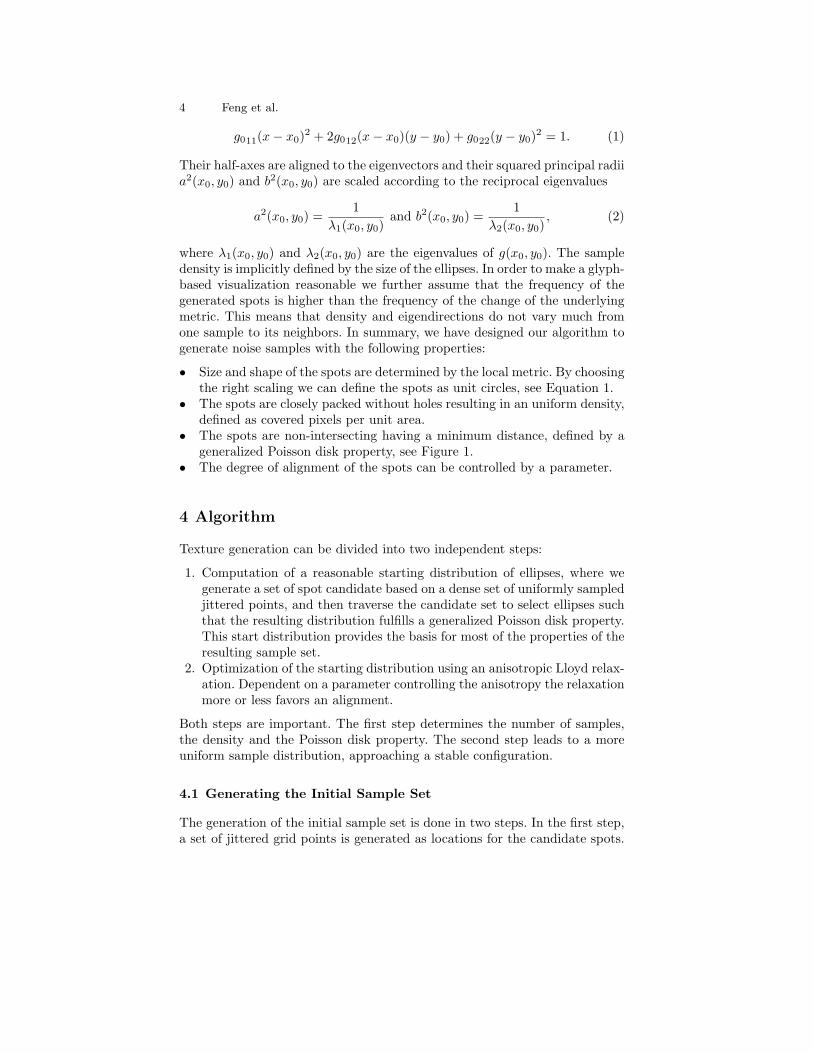
Fig. 1. Generalized Poisson disk property. The minimum distance of two samplepoints is defined by the local ellipses, which are not allowed to overlap.

The use of glyphs for visualization of local field properties is common invisualization. The question of placing these glyphs has been subject of discus-sion in several contexts. The most common strategies are regular sampling,random sampling with or without Poisson property [17, 13] or proceduraltexture generation, e.g., using reaction diffusion. In vector field visualization,Turk and Banks proposed a method to place arrows along streamlines gener-ated by streamline optimization [23]. Kindlmann introduced reaction-diffusioninto the visualization community applying it to diffusion tensor MRI data [11].Sanderson et al. used a reaction-diffusion model to generate spot noise basedon the underlying vector field placing glyphs at the spot center [21]. Reactiondiffusion provides automatic control of density, size and placement of patternsbut the specification of appropriate parameters is not trivial. Stable patternsonly form for a very narrow band of values for the parameters. In addition it iscomputationally expensive. Recently Kindlman and Westin proposed a glyphpacking algorithm in the context of diffusion tensor visualization [12]. Theirwork is built on a particle approach simulating attractive and repulsive forces.This work is an extension to our recent work for the generation of anisotropicnoise samples [3] by adding a control over the alignment of the ellipses.

3 Assumptions and Goals

The starting point for the generation of the elliptic noise samples is a metricg = (gij) given over a domain D ⊂ R2, which defines the sample properties.The metric can be user-defined or derived from scalar fields, vector fields, ortensor fields, see Section 6. The metric is given as a two-by-two symmetric,positive definite matrix depending on the location P = (x, y) ∈ R2. We assumethat the metric is non-degenerate everywhere. In general, it is spatially varyingand anisotropic. Size and density of the ellipses are specified by the metric intheir center P0 = (x0, y0). Their shape is defined as unit circle with respectto the metric g0 in P0, i.e.,

4 Feng et al.

g011(x− x0)2 + 2g012(x− x0)(y − y0) + g022(y − y0)2 = 1. (1)

Their half-axes are aligned to the eigenvectors and their squared principal radiia2(x0, y0) and b2(x0, y0) are scaled according to the reciprocal eigenvalues

a2(x0, y0) =1

λ1(x0, y0)and b2(x0, y0) =

1λ2(x0, y0)

, (2)

where λ1(x0, y0) and λ2(x0, y0) are the eigenvalues of g(x0, y0). The sampledensity is implicitly defined by the size of the ellipses. In order to make a glyph-based visualization reasonable we further assume that the frequency of thegenerated spots is higher than the frequency of the change of the underlyingmetric. This means that density and eigendirections do not vary much fromone sample to its neighbors. In summary, we have designed our algorithm togenerate noise samples with the following properties:

• Size and shape of the spots are determined by the local metric. By choosingthe right scaling we can define the spots as unit circles, see Equation 1.

• The spots are closely packed without holes resulting in an uniform density,defined as covered pixels per unit area.

• The spots are non-intersecting having a minimum distance, defined by ageneralized Poisson disk property, see Figure 1.

• The degree of alignment of the spots can be controlled by a parameter.

4 Algorithm

Texture generation can be divided into two independent steps:

1. Computation of a reasonable starting distribution of ellipses, where wegenerate a set of spot candidate based on a dense set of uniformly sampledjittered points, and then traverse the candidate set to select ellipses suchthat the resulting distribution fulfills a generalized Poisson disk property.This start distribution provides the basis for most of the properties of theresulting sample set.

2. Optimization of the starting distribution using an anisotropic Lloyd relax-ation. Dependent on a parameter controlling the anisotropy the relaxationmore or less favors an alignment.

Both steps are important. The first step determines the number of samples,the density and the Poisson disk property. The second step leads to a moreuniform sample distribution, approaching a stable configuration.

4.1 Generating the Initial Sample Set

The generation of the initial sample set is done in two steps. In the first step,a set of jittered grid points is generated as locations for the candidate spots.


The initial set must have higher density than the target density. target den-sity leads to good results. The candidate spots in each location are definedby the local metric as “unit-circle.” For a general metric g, these are ellipsesdefined by Equation 1. At this stage, the generated candidate spots generallyoverlap. Once the initial set of points is generated, the algorithm traverses theset of points. A candidate spot is accepted when its ellipse does not overlapwith the ellipses at any other already selected samples. The underlying regulargrid structure of random points has the nice property that it supports effi-cient spatial search of neighboring points, therefore simplifying the checkingprocess.

4.2 Anisotropic Voronoi Relaxation

By eliminating overlapping samples, holes can result in certain areas. To re-move these artifacts we use a method similar to Lloyd relaxation.

Lloyd relaxation (also known as Voronoi iteration) is a method to generateevenly distributed samples. It is an iteration of constructing Voronoi tessella-tion and its centroids. In each iteration the sample points are moved into thecell centroid, which corresponds to the center of mass of the cell. The processconverges against a centroidal Voronoi diagram, where each sample point liesin its cell centroid. This diagram minimizes the energy given as

E =∑i∈I

∫V ori

ρ(x)||r − ri||2dr (3)

where I is the index set for the samples, V ori the Voronoi cell of the ithsample, ri its position and ρ a local scalar density.

Due to the anisotropy of the metric, we use an anisotropic Voronoi dia-gram and an anisotropic centroid computation for the relaxation step. For thedefinition of the anisotropic Voronoi diagram and the centroid computationwe built on the works of Labelle and Shewchuk [16] and Du et al. [2]. Ourmethod is a combination of these two methods, satisfying our demands. De-pending on the special choice of the metric used to define the Voronoi cellsthe alignment of ellipses is more or less supported.

Definition of the Voronoi regions

Let {Pi ∈ D, i ∈ I} be the set of sample points resulting from our previousstep, where I is an index set for the points. The most natural way of general-izing the Voronoi tessellation to other more general metrics would be to definea Voronoi cell Vor(Pi) of a point Pi as the set of all points P ∈ D that are atleast as close to Pi as to any other point Pj , j 6= i, using the geodesic insteadof the Euclidean distance. However, since the computation of this shortestpath is difficult and computationally expensive we use an approximate dis-tance function for two points proposed by Labelle and Shewchuk, because itmatches our conditions well, i.e.,

6 Feng et al.

d2(P,Q) = (P −Q)T g(P )(P −Q). (4)

The distance measure is not symmetric d(P,Q) 6= d(Q,P ). Also, the triangleinequality is not necessarily satisfied. Based on this approximate distance, aVoronoi cell of point Pi is defined as

V or(Pi) = {P ∈ D|d(Pi, P ) ≤ d(Pj , P ) for all j ∈ I with i 6= j. (5)

When using the metric defining the ellipses, this distance function guaranteesthat ellipses of our start configuration lie entirely inside the Voronoi cells.The resulting Voronoi cells are in general not convex and may not even beconnected. Therefore, we define a localized version of the Voronoi cells con-sidering only the part containing the sample point. For more details we referto [3]. We define

V orr(Pi) = {P ∈ D|i ∈ IP and d(Pi, P ) ≤ d(Pj , P ) for all j ∈ IP with i 6= j,

with IP = {i ∈ I|(Pi − Pj) · (P − Pi) ≤ 0,∀j 6= i}. (6)

Centroid definition

For the definition of the centroid we follow the idea of Du et al. [2], which isa straight-forward generalization of centroid definition as the center of massto an anisotropic setting. The center of mass ci of a Voronoi cell V or(Pi) isdefined as

ci =

∫V or(Pi)

d(r)r dr∫V or(Pi)

d(r) dr, (7)

where d is an isotropic scalar density and r = (x, y). By replacing the densityd by the metric tensor g the centroid ci is defined as

ci =

(∫V or(Pi)

g(r) dr

)−1

·

(∫V or(Pi)

g(r) · r dr

). (8)

As an integral over positive definite matrices, the left matrix is always invert-ible. When using an isotropic metric this definition reduces to the standardweighted centroid definition. If the metric is uniform, i.e., it does not dependon r, the anisotropic centroid definition coincides with isotropic uniform case.

4.3 Implementation

Intersection test

The initial sampling requires intersection tests between neighboring samples.In the isotropic case, this intersection test is simply the circle to circle intersec-tion test and can be done efficiently. In the more general case, the samples arerepresented by ellipses. The algebraic method of ellipse to ellipse intersectiontest involve solving a quadratic polynomial, which is computationally expen-sive and numerically unstable. We use polylines to approximate the ellipsesduring intersection test to reduce complexity. This approximation producesgood results without the issues involved in the algebraic method.


Relaxation

For the computation of the Voronoi cells and the centroid we use a discreteapproach. Considering the domain as a set of uniform cells represented bytheir center R the discretized of Equation 8 results in

ci − Pi︸︷︷︸≡Ti

=

∑R∈V or(Pi)

g(R)

︸︷︷︸

≡Mi

−1 ·∑

R∈V or(Pi)

g(R) · (R− Pi)︸︷︷︸≡ti

(9)

Instead of computing the Voronoi cell explicitly and using these cells forthe centroid computation, we perform both computations in one step. Weinitialize all sample positions Pi, i ∈ I, with a zero vector ti and zero matrixMi. Next, we march through the discretized domain performing the followingsteps for each cell represented by the point R:

• Find the Voronoi Cell V orr(Pi) containing point R to specify i, by com-paring the distances to sample points lying inside a local bin.

• Update the matrix Mi and the vector ti in the following way:

Mi → Mi + g(R)ti → ti + g(R) · (R− Pi)

(10)

After traversing the entire domain, the new position of the sample points Pi,given by Equation 9, is determined by the translation vector Ti, i.e.,

Ti = M−1 · ti and Pi → P ′i = Pi + Ti. (11)

5 Structural Behavior

The distance approximation makes general statements about the convergencebehavior of the point set difficult. But we can identify fix-points of the re-laxation process for the uniform case, as e.g., hexagonal structures or anyother point symmetric configurations. In our examples we observe that afterseveral iterations regions with hexagonal patterns are forming, see Figure 2.Inside these regions the patterns become soon relatively stable. Between theseregions the structure still changes slightly even after many iterations.

Dependent on the orientation of the ellipses in relation to the orientation ofthe hexagonal structure, these configurations result in an aligned structure ornot. A similar behavior can be observed for slowly varying fields. Whether analignment is desirable depends on the specific application. While it generatesartifacts when the samples are used as input for texture generation or in non-photorelalistic rendering applications, it enhances perception of flow field datasets.

8 Feng et al.

(a) (b) (c)

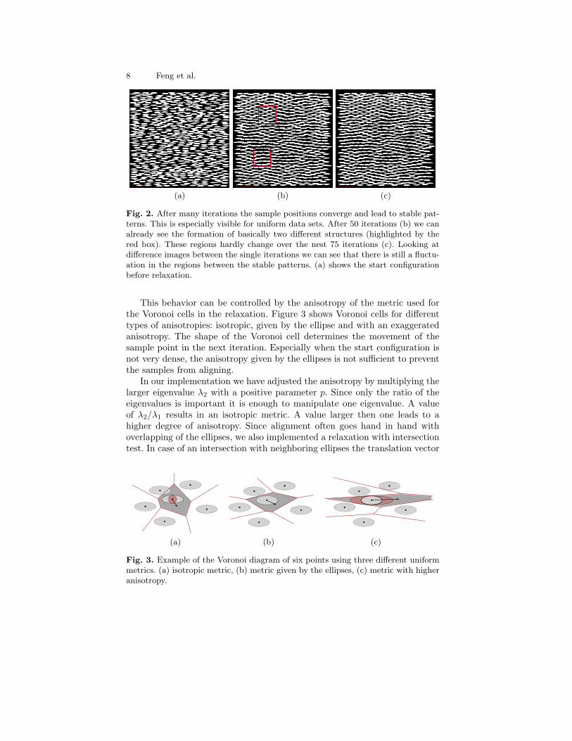
Fig. 2. After many iterations the sample positions converge and lead to stable pat-terns. This is especially visible for uniform data sets. After 50 iterations (b) we canalready see the formation of basically two different structures (highlighted by thered box). These regions hardly change over the nest 75 iterations (c). Looking atdifference images between the single iterations we can see that there is still a fluctu-ation in the regions between the stable patterns. (a) shows the start configurationbefore relaxation.

This behavior can be controlled by the anisotropy of the metric used forthe Voronoi cells in the relaxation. Figure 3 shows Voronoi cells for differenttypes of anisotropies: isotropic, given by the ellipse and with an exaggeratedanisotropy. The shape of the Voronoi cell determines the movement of thesample point in the next iteration. Especially when the start configuration isnot very dense, the anisotropy given by the ellipses is not sufficient to preventthe samples from aligning.

In our implementation we have adjusted the anisotropy by multiplying thelarger eigenvalue λ2 with a positive parameter p. Since only the ratio of theeigenvalues is important it is enough to manipulate one eigenvalue. A valueof λ2/λ1 results in an isotropic metric. A value larger then one leads to ahigher degree of anisotropy. Since alignment often goes hand in hand withoverlapping of the ellipses, we also implemented a relaxation with intersectiontest. In case of an intersection with neighboring ellipses the translation vector

(a) (b) (c)

Fig. 3. Example of the Voronoi diagram of six points using three different uniformmetrics. (a) isotropic metric, (b) metric given by the ellipses, (c) metric with higheranisotropy.


(a) (b)

(c) (d)

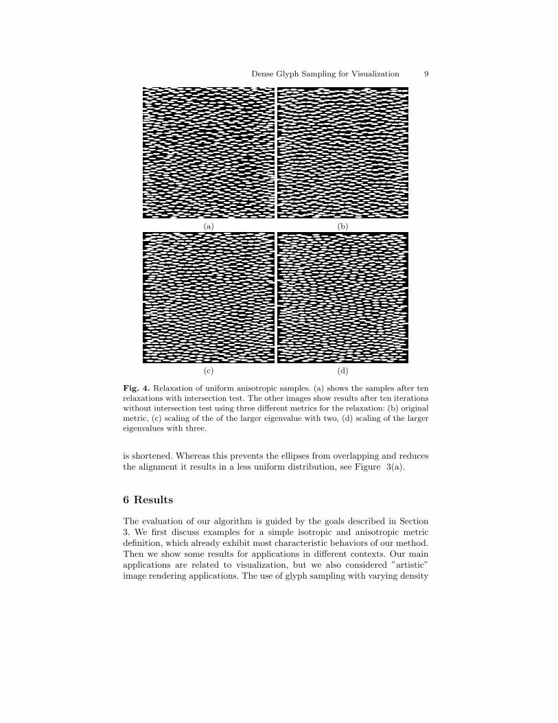
Fig. 4. Relaxation of uniform anisotropic samples. (a) shows the samples after tenrelaxations with intersection test. The other images show results after ten iterationswithout intersection test using three different metrics for the relaxation: (b) originalmetric, (c) scaling of the of the larger eigenvalue with two, (d) scaling of the largereigenvalues with three.

is shortened. Whereas this prevents the ellipses from overlapping and reducesthe alignment it results in a less uniform distribution, see Figure 3(a).

6 Results

The evaluation of our algorithm is guided by the goals described in Section3. We first discuss examples for a simple isotropic and anisotropic metricdefinition, which already exhibit most characteristic behaviors of our method.Then we show some results for applications in different contexts. Our mainapplications are related to visualization, but we also considered ”artistic”image rendering applications. The use of glyph sampling with varying density

10 Feng et al.

(a) (b) (c)

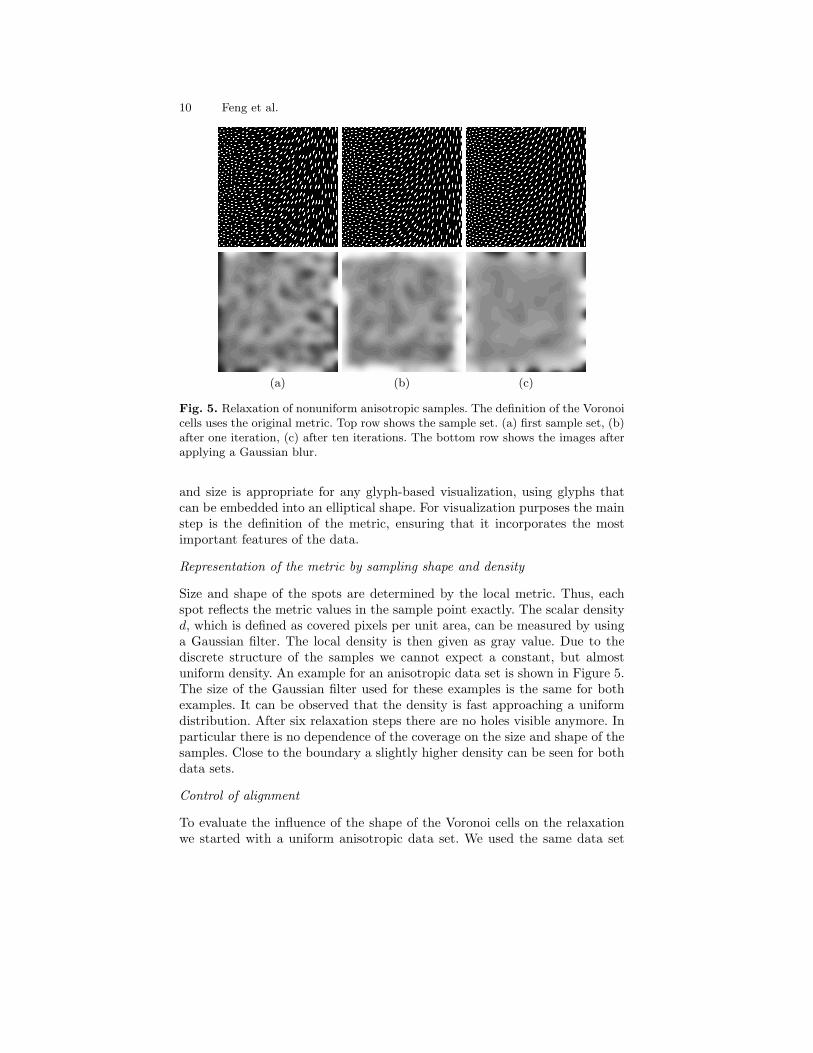
Fig. 5. Relaxation of nonuniform anisotropic samples. The definition of the Voronoicells uses the original metric. Top row shows the sample set. (a) first sample set, (b)after one iteration, (c) after ten iterations. The bottom row shows the images afterapplying a Gaussian blur.

and size is appropriate for any glyph-based visualization, using glyphs thatcan be embedded into an elliptical shape. For visualization purposes the mainstep is the definition of the metric, ensuring that it incorporates the mostimportant features of the data.

Representation of the metric by sampling shape and density

Size and shape of the spots are determined by the local metric. Thus, eachspot reflects the metric values in the sample point exactly. The scalar densityd, which is defined as covered pixels per unit area, can be measured by usinga Gaussian filter. The local density is then given as gray value. Due to thediscrete structure of the samples we cannot expect a constant, but almostuniform density. An example for an anisotropic data set is shown in Figure 5.The size of the Gaussian filter used for these examples is the same for bothexamples. It can be observed that the density is fast approaching a uniformdistribution. After six relaxation steps there are no holes visible anymore. Inparticular there is no dependence of the coverage on the size and shape of thesamples. Close to the boundary a slightly higher density can be seen for bothdata sets.

Control of alignment

To evaluate the influence of the shape of the Voronoi cells on the relaxationwe started with a uniform anisotropic data set. We used the same data set


as for Figure 2, where the initial sample set can be seen in (a). Figure 4shows results using different relaxation methods after ten iterations. For thegeneration of Figure 4(a) and (b) the Voronoi cells are computed using theoriginal metric as given by the ellipses. In (a) we performed an intersectiontest after each iteration. This enforces the maintenance of the Poisson diskproperty but also hinders the relaxation process. There are holes in the dataseteven after ten iterations. (b) shows the result without intersection test. Wecan observe hexagonal structures with and without alignment of the ellipses.There almost no holes left, but there are a few regions where the ellipses startoverlapping. For Figure 4(c) and (d) we used an exaggerated anisotropy forthe Voronoi cell computation. Especially (d) shows a very uniform structurewith almost no overlapping and alignment along the major eigenvector.

Vector field visualization

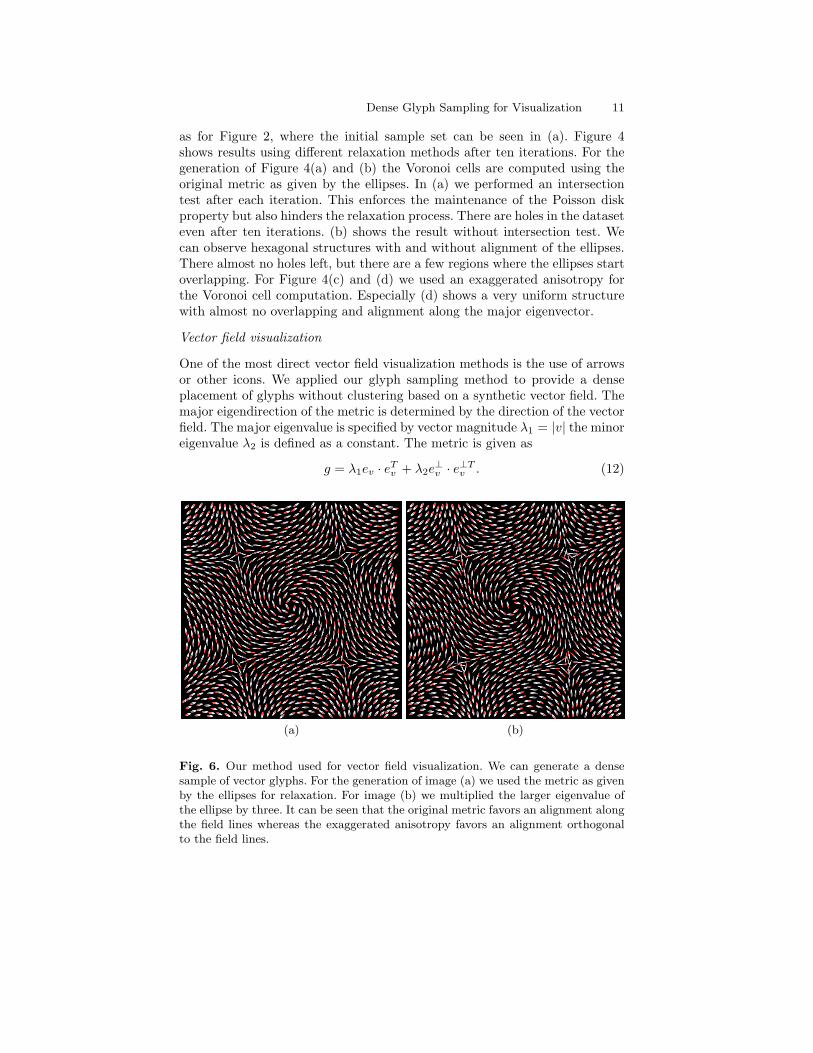
One of the most direct vector field visualization methods is the use of arrowsor other icons. We applied our glyph sampling method to provide a denseplacement of glyphs without clustering based on a synthetic vector field. Themajor eigendirection of the metric is determined by the direction of the vectorfield. The major eigenvalue is specified by vector magnitude λ1 = |v| the minoreigenvalue λ2 is defined as a constant. The metric is given as

g = λ1ev · eTv + λ2e

⊥v · e⊥T

v . (12)

(a) (b)

Fig. 6. Our method used for vector field visualization. We can generate a densesample of vector glyphs. For the generation of image (a) we used the metric as givenby the ellipses for relaxation. For image (b) we multiplied the larger eigenvalue ofthe ellipse by three. It can be seen that the original metric favors an alignment alongthe field lines whereas the exaggerated anisotropy favors an alignment orthogonalto the field lines.

12 Feng et al.

Figure 6 shows the results for two different degrees of anisotropy in the re-laxation after five iterations. The left image uses the original metric g, in theright image the larger eigenvalue is scaled by a factor of three. Both imagesshow a uniform sampling of the ellipses, but the perception of flow is muchbetter in (a). To achieve similar results Turk and Banks proposed a method toplace arrows along streamlines generated using streamline optimization [23].Sanderson et al. [21] used a reaction-diffusion model to generate spot noisebased on the underlying vector field, and places glyphs at spot centers.

Tensor field visualization

To be able to use anisotropic noise for the visualization of tensor data, wemust define a metric based on the given tensors. Some of the tensor fields weare interested in are already positive definite, e.g., diffusion tensor fields. Butother tensor fields, like stress or strain fields, also have negative eigenvalues.To be able to treat such tensor fields we interpret them as distortion of a flatmetric [9]. Assume that we have a positive definite tensor field T defined overa domain D. Let λ1 and λ2 be its eigenvalues and v1 and v2 the respectiveeigenvectors. We define the metric for the sample generation as

g =1√λ1

v1 · vT1 +

1√λ2

v2 · vT2 (13)

(a) (b)

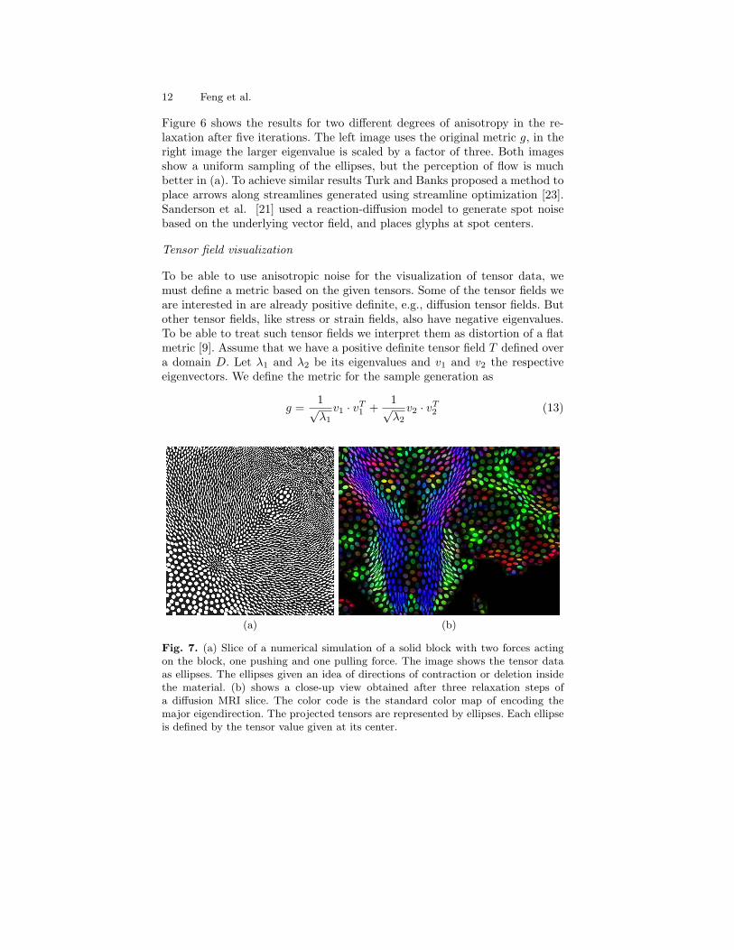
Fig. 7. (a) Slice of a numerical simulation of a solid block with two forces actingon the block, one pushing and one pulling force. The image shows the tensor dataas ellipses. The ellipses given an idea of directions of contraction or deletion insidethe material. (b) shows a close-up view obtained after three relaxation steps ofa diffusion MRI slice. The color code is the standard color map of encoding themajor eigendirection. The projected tensors are represented by ellipses. Each ellipseis defined by the tensor value given at its center.


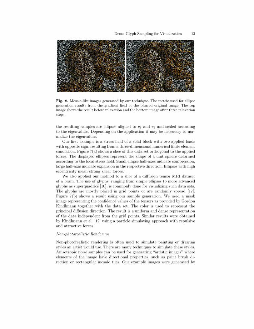
Fig. 8. Mosaic-like images generated by our technique. The metric used for ellipsegeneration results from the gradient field of the blurred original image. The topimage shows the result before relaxation and the bottom image after three relaxationsteps.

the resulting samples are ellipses aligned to v1 and v2 and scaled accordingto the eigenvalues. Depending on the application it may be necessary to nor-malize the eigenvalues.

Our first example is a stress field of a solid block with two applied loadswith opposite sign, resulting from a three-dimensional numerical finite elementsimulation. Figure 7(a) shows a slice of this data set orthogonal to the appliedforces. The displayed ellipses represent the shape of a unit sphere deformedaccording to the local stress field. Small ellipse half-axes indicate compression,large half-axis indicate expansion in the respective direction. Ellipses with higheccentricity mean strong shear forces.

We also applied our method to a slice of a diffusion tensor MRI datasetof a brain. The use of glyphs, ranging from simple ellipses to more advancedglyphs as superquadrics [10], is commonly done for visualizing such data sets.The glyphs are mostly placed in grid points or are randomly spread [17].Figure 7(b) shows a result using our sample generation. We used a maskimage representing the confidence values of the tensors as provided by GordonKindlmann together with the data set. The color is used to represent theprincipal diffusion direction. The result is a uniform and dense representationof the data independent from the grid points. Similar results were obtainedby Kindlmann et al. [12] using a particle simulating approach with repulsiveand attractive forces.

Non-photorealistic Rendering

Non-photorealistic rendering is often used to simulate painting or drawingstyles an artist would use. There are many techniques to simulate these styles.Anisotropic noise samples can be used for generating “artistic images” whereelements of the image have directional properties, such as paint brush di-rection or rectangular mosaic tiles. Our example images were generated by

14 Feng et al.

constructing a gradient vector field based on the intensity values of the im-ages. To reduce noise in the vector field, the original images were blurred byapplying a Gaussian filter. We defined a tensor metric over the image usingthe gradient vector field and its orthogonal vector field. The orthogonal vec-tor field essentially points in the direction tangent to the boundary featuresin the images. One example can be seen in Figure 8, the left image showsthe ellipses before relaxation the right image after three relaxations using theoriginal metric.

7 Conclusion

We have introduced a method to generate a dense set of uniformly spreadglyphs. Besides the local control of size and density the methods provides aparameter to control the alignment of the glyphs. size. This is a desirableproperty not only in tensor field visualization. As for all glyph-based methodsthe resolution of the representation is limited by the size of the glyphs thatare used.

Our method is a purely geometric process. The centroid can be computedexplicitly without involving numerics. In contrast to models using repulsiveforces the Voronoi cell based relaxation is very stable. Using a good startconfiguration of the samples only a few relaxation steps are needed to achievea uniform distribution. Thus the method is reasonable fast.

Due to the lack of repulsive forces the Voronoi relaxation does not neces-sarily preserve the Poisson disk property. We have shown that we can reducethe violation of the Poisson disk property by manipulating the shape of theVoronoi cell appropriately. The key entity thereby is the anisotropy of themetric used for the Voronoi cell definition. In contrast to expensive intersec-tion tests, this approach does not hinder the relaxation process and does notintroduce any additional computational costs.

Acknowledgments

The brain dataset is courtesy of Gordon Kindlmann, Scientific Computingand Imaging Institute, University of Utah, and Andrew Alexander, W. M.Keck Laboratory for Functional Brain Imaging and Behavior, University ofWisconsin-Madison. This work was supported by the National Science Foun-dation under contracts ACI 9624034 (CAREER Award), through the LargeScientific and Software Data Set Visualization (LSSDSV) program under con-tract ACI 9982251, and a large Information Technology Research (ITR) grant;the National Institutes of Health under contract P20 MH60975-06A2, fundedby the National Institute of Mental Health and the National Science Foun-dation; and the U.S. Bureau of Reclamation. We gratefully acknowledge thesupport of the W.M. Keck Foundation provided to the UC Davis Center for


Active Visualization in the Earth Sciences (CAVES). We thank the membersof the Visualization and Computer Graphics Research Group at the Institutefor Data Analysis and Visualization (IDAV) at the University of California,Davis.

References

1. Q. Du, V. Faber, and M. Gunzburger. Centroidal voronoi tessellations: Appli-cations and algorithms. SIAM Review, 41(4):637–676, 1999.

2. Q. Du and D. Wang. Anisotropic centroidal voronoi tessellations and theirapplications. SIAM Journal on Scientific Computing, 26(3):737–761, 2005.

3. L. Feng, I. Hotz, B. Hamann, and K. I. Joy. Anisotropic noise samples. IEEETransactions on Visualization and Computer Graphics, oct submitted 2006.

4. L.-P. Fritzsche, H. Hellwig, S. Hiller, and O. Deussen. Interactive design ofauthentic looking mosaics using voronoi structures. In Proceedings of 2nd Inter-national Symposium on Voronoi Diagrams in Science and Engineering, Seoul,Korea, 2005.

5. A. S. Glassner. Principles of Digital Image Synthesis: Volume Two. The Mor-gan Kaufmann Series in Computer Graphics and Geometric Modeling. MorganKaufmann, 1995. GLA a 95:2 1.Ex.

6. A. Hausner. Simulating decorative mosaics. In E. Fiume, editor, SIGGRAPH2001, Computer Graphics Proceedings, pages 573–578, 2001.

7. S. Hiller, H. Hellwig, and O. Deussen. Beyond stippling - methods for distribut-ing objects on the plane. Comput. Graph. Forum, 22(3):515–522, 2003.

8. A. J. S. Hin and F. H. Post. Visualization of turbulent flow with particles. InVIS ’93: Proceedings of the 4th conference on Visualization ’93, pages 46–53,1993.

9. I. Hotz, L. Feng, H. Hagen, B. Hamann, B. Jeremic, and K. I. Joy. Physicallybased methods for tensor field visualization. In Proceedings of IEEE Visualiza-tion 2004, pages 123–130. IEEE Computer Society Press, oct 2004.

10. G. Kindlmann. Superquadric tensor glyphs. In Proceeding of The Joint Euro-graphics - IEEE TCVG Symposium on Visualization, pages 147–154, May 2004.

11. G. Kindlmann, D. Weinstein, and D. Hart. Strategies for direct volume renderingof diffusion tensor fields. IEEE Transactions on Visualization and ComputerGraphics, 6(2):124–138, /2000.

12. G. Kindlmann and C.-F. Westin. Diffusion tensor visualization with glyph pack-ing. IEEE Transactions on Visualization and Computer Graphics (ProceedingsVisualization / Information Visualization 2006), 12(5):(to appear), September-October 2006.

13. R. M. Kirby, H. Marmanis, and D. H. Laidlaw. Visualizing multivalued datafrom 2D incompressible flows using concepts from painting. In D. Ebert,M. Gross, and B. Hamann, editors, IEEE Visualization ’99, pages 333–340,San Francisco, 1999.

14. M.-H. Kiu and D. C. Banks. Multi-frequency noise for lic. In VIS ’96: Proceed-ings of the 7th conference on Visualization ’96, pages 121–126, Los Alamitos,CA, USA, 1996. IEEE Computer Society Press.

15. D. E. Knuth. Digital halftones by dot diffusion. ACM Transactions on Graphics,6(4):245–273, 1987.

16 Feng et al.

16. F. Labelle and J. R. Shewchuk. Anisotropic voronoi diagrams and guaranteed-quality anisotropic mesh generation. In SCG ’03: Proceedings of the nineteenthannual symposium on Computational geometry, pages 191–200, New York, NY,USA, 2003. ACM Press.

17. D. H. Laidlaw, E. T. Ahrens, D. Kremers, M. J. Avalos, R. E. Jacobs, andC. Readhead. Visualizing diffusion tensor images of the mouse spinal cord. InD. Ebert, H. Hagen, and H. Rushmeier, editors, IEEE Visualization ’98 (VIS’98), pages 127–134, Washington - Brussels - Tokyo, Oct. 1998. IEEE, IEEEComputer Society Press.

18. S. P. Lloyd. Least square quantization in pcm. IEEE Transactions on Informa-tion Theory, 28(2):129–137, Mar. 1982.

19. V. Ostromoukhov. A simple and efficient error-diffusion algorithm. In Pro-ceedings of the 28th annual conference on Computer graphics and interactivetechniques, pages 567–572. ACM Press, 2001.

20. V. Ostromoukhov, C. Donohue, and P.-M. Jodoin. Fast hierarchical importancesampling with blue noise properties. ACM Trans. Graph., 23(3):488–495, 2004.

21. A. R. Sanderson, C. R. Johnson, and R. M. Kirby. Display of vector fieldsusing a reaction-diffusion model. In VIS ’04: Proceedings of the conference onVisualization ’04, pages 115–122, Washington, DC, USA, 2004. IEEE ComputerSociety.

22. K. Shimada, A. Yamada, and T. Itoh. Anisotropic triangulation of paramet-ric surfaces via close packing of ellipsoids. Int. J. Comput. Geometry Appl.,10(4):417–440, 2000.

23. G. Turk and D. Banks. Image-guided streamline placement. Computer Graphics,30(Annual Conference Series):453–460, 1996.

24. R. Ulichney. Digital halftoning. MIT Press, Cambridge, MA, USA, 1987.25. L. Velho and J. de Miranda Gomes. Digital halftoning with space filling curves.

In Proceedings of the 18th annual conference on Computer graphics and inter-active techniques, pages 81–90. ACM Press, 1991.

Dense Glyph Sampling for Visualization

Documents