Denoising by Sparse Approximation: Error Bounds Based on Rate-Distortion Theory

Hindawi Publishing CorporationEURASIP Journal on Applied Signal ProcessingVolume 2006, Article ID 26318, Pages 1–19DOI 10.1155/ASP/2006/26318

Denoising by Sparse Approximation: Error BoundsBased on Rate-Distortion Theory

Alyson K. Fletcher,1 Sundeep Rangan,2 Vivek K Goyal,3 and Kannan Ramchandran4

1 Department of Electrical Engineering and Computer Sciences, University of California, Berkeley, CA 94720-1770, USA2 Flarion Technologies Inc., Bedminster, NJ 07921, USA3 Department of Electrical Engineering and Computer Science and Research Laboratory of Electronics,Massachusetts Institute of Technology, Cambridge, MA 02139-4307, USA

4 Department of Electrical Engineering and Computer Sciences, College of Engineering, University of California, Berkeley,CA 94720-1770, USA

Received 9 September 2004; Revised 6 June 2005; Accepted 30 June 2005

If a signal x is known to have a sparse representation with respect to a frame, it can be estimated from a noise-corrupted observationy by finding the best sparse approximation to y. Removing noise in this manner depends on the frame efficiently representing thesignal while it inefficiently represents the noise. The mean-squared error (MSE) of this denoising scheme and the probabilitythat the estimate has the same sparsity pattern as the original signal are analyzed. First an MSE bound that depends on a newbound on approximating a Gaussian signal as a linear combination of elements of an overcomplete dictionary is given. Furtheranalyses are for dictionaries generated randomly according to a spherically-symmetric distribution and signals expressible withsingle dictionary elements. Easily-computed approximations for the probability of selecting the correct dictionary element andthe MSE are given. Asymptotic expressions reveal a critical input signal-to-noise ratio for signal recovery.

Copyright © 2006 Alyson K. Fletcher et al. This is an open access article distributed under the Creative Commons AttributionLicense, which permits unrestricted use, distribution, and reproduction in any medium, provided the original work is properlycited.

1. INTRODUCTION

Estimating a signal from a noise-corrupted observation ofthe signal is a recurring task in science and engineering. Thispaper explores the limits of estimation performance in thecase where the only a priori structure on the signal x ∈ RN

is that it has known sparsity K with respect to a given set ofvectors Φ = {ϕi}Mi=1 ⊂ RN . The set Φ is called a dictionaryand is generally a frame [1, 2]. The sparsity of K with respectto Φ means that the signal x lies in the set

ΦK ={v ∈ RN | v =

M∑i=1

αiϕi with at most K nonzero αi’s

}.

(1)

In many areas of computation, exploiting sparsity is mo-tivated by reduction in complexity [3]; if K � N , then cer-tain computations may be more efficiently made on α thanon x. In compression, representing a signal exactly or approx-imately by a member of ΦK is a common first step in effi-ciently representing the signal, though much more is knownwhen Φ is a basis or union of wavelet bases than is knownin the general case [4]. Of more direct interest here is that

sparsity models are becoming prevalent in estimation prob-lems; see, for example, [5, 6].

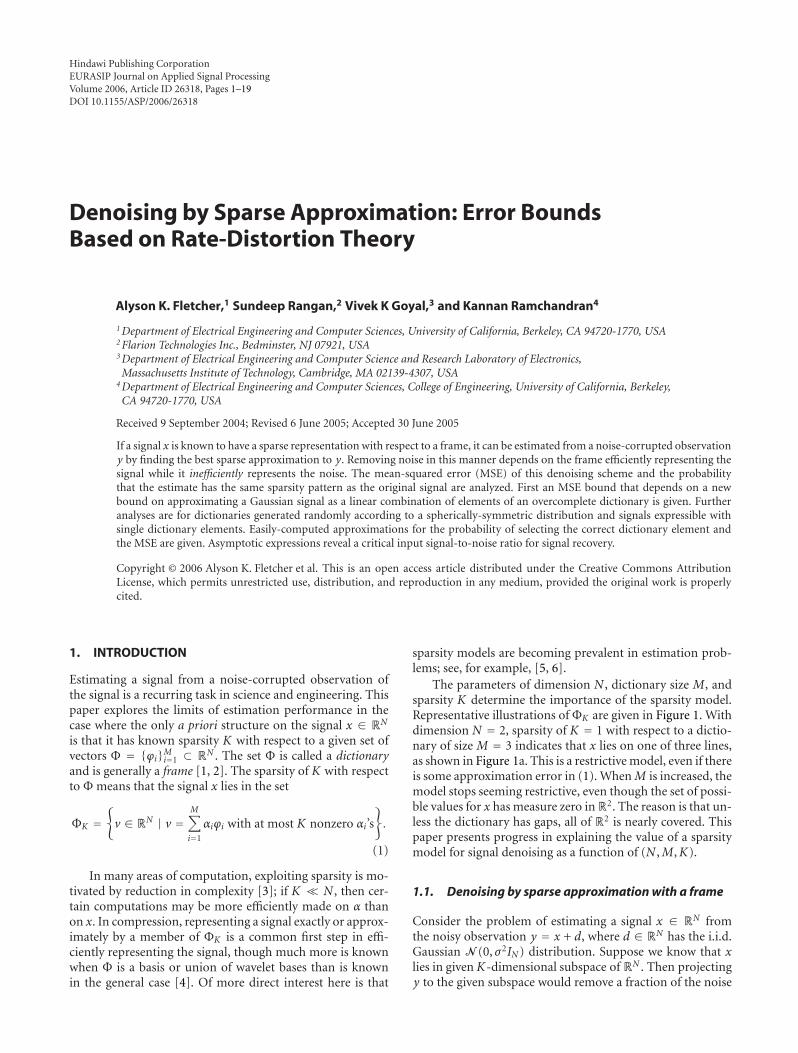
The parameters of dimension N , dictionary size M, andsparsity K determine the importance of the sparsity model.Representative illustrations of ΦK are given in Figure 1. Withdimension N = 2, sparsity of K = 1 with respect to a dictio-nary of size M = 3 indicates that x lies on one of three lines,as shown in Figure 1a. This is a restrictive model, even if thereis some approximation error in (1). When M is increased, themodel stops seeming restrictive, even though the set of possi-ble values for x has measure zero inR2. The reason is that un-less the dictionary has gaps, all of R2 is nearly covered. Thispaper presents progress in explaining the value of a sparsitymodel for signal denoising as a function of (N ,M,K).

1.1. Denoising by sparse approximation with a frame

Consider the problem of estimating a signal x ∈ RN fromthe noisy observation y = x + d, where d ∈ RN has the i.i.d.Gaussian N (0, σ2IN ) distribution. Suppose we know that xlies in given K-dimensional subspace of RN . Then projectingy to the given subspace would remove a fraction of the noise

2 EURASIP Journal on Applied Signal Processing

(a) (b)

Figure 1: Two sparsity models in dimension N = 2. (a) Havingsparsity K = 1 with respect to a dictionary with M = 3 elementsrestricts the possible signals greatly. (b) With the dictionary size in-creased to M = 100, the possible signals still occupy a set of measurezero, but a much larger fraction of signals is approximately sparse.

without affecting the signal component. Denoting the pro-jection operator by P, we would have

x = Py = P(x + d) = Px + Pd = x + Pd, (2)

and Pd has only K/N fraction of the power of d.In this paper, we consider the more general signal model

x ∈ ΦK . The set ΦK defined in (1) is the union of at mostJ = (

MK

)subspaces of dimension K . We henceforth assume

that M > K (thus J > 1); if not, the model reduces to theclassical case of knowing a single subspace that contains x.The distribution of x, if available, could also be exploited toremove noise. However, in this paper the denoising operationis based only on the geometry of the signal model ΦK and thedistribution of d.

With the addition of the noise d, the observed vector ywill (almost surely) not be represented sparsely, that is, not bein ΦK . Intuitively, a good estimate for x is the point from ΦK

that is closest to y in Euclidean distance. Formally, becausethe probability density function of d is a strictly decreasingfunction of ‖d‖2, this is the maximum-likelihood estimateof x given y. The estimate is obtained by applying an optimalsparse approximation procedure to y. We will write

xSA = arg minx∈ΦK

‖y − x‖2 (3)

for this estimate and call it the optimal K-term approxima-tion of y. Henceforth, we omit the subscript 2 indicating theEuclidean norm.

The main results of this paper are bounds on the per-component mean-squared estimation error (1/N)E[‖x −xSA‖2] for denoising via sparse approximation.1 Thesebounds depend on (N ,M,K) but avoid further dependenceon the dictionary Φ (such as the coherence of Φ); some re-sults hold for all Φ and others are for randomly generated Φ.

1 The expectation is always over the noise d and is over the dictionary Φand signal x in some cases. However, the estimator does not use the dis-tribution of x.

To the best of our knowledge, the results differ from any inthe literature in several ways.

(a) We study mean-squared estimation error for additiveGaussian noise, which is a standard approach to per-formance analysis in signal processing. In contrast,analyses such as [7] impose a deterministic bound onthe norm of the noise.

(b) We concentrate on having dependence solely on dic-tionary size rather than more fine-grained propertiesof the dictionary. In particular, most signal recov-ery results in the literature are based on noise beingbounded above by a function of the coherence of thedictionary [8–14].

(c) Some of our results are for spherically symmetric ran-dom dictionaries. The series of papers [15–17] is su-perficially related because of randomness, but in thesepapers, the signals of interest are sparse with respect toa single known, orthogonal basis and the observationsare random inner products. The natural questions in-clude a consideration of the number of measurementsneeded to robustly recover the signal.

(d) We use source-coding thought experiments in bound-ing estimation performance. This technique may beuseful in answering other related questions, especiallyin sparse approximation source coding.

Our preliminary results were first presented in [18], with fur-ther details in [19, 20]. Probability of error results in a ratherdifferent framework for basis pursuit appear in a manuscriptsubmitted while this paper was under review [21].

1.2. Connections to approximation

A signal with an exact K-term representation might arise be-cause it was generated synthetically, for example, by a com-pression system. A more likely situation in practice is thatthere is an underlying true signal x that has a good K-termapproximation rather than an exact K-term representation. Atvery least, this is the goal in designing the dictionary Φ for asignal class of interest. It is then still reasonable to compute(3) to estimate x from y, but there are tradeoffs in the selec-tions of K and M.

Let fM,K denote the squared Euclidean approximationerror of the optimal K-term approximation using an M-element dictionary. It is obvious that fM,K decreases with in-creasing K , and with suitably designed dictionaries, it alsodecreases with increasing M. One concern of approxima-tion theory is to study the decay of fM,K precisely. (For this,we should consider N very large or infinite.) For piecewisesmooth signals, for example, wavelet frames give exponentialdecay with K [4, 22, 23].

When one uses sparse approximation to denoise, the per-formance depends on both the ability to approximate x andthe ability to reject the noise. Approximation is improvedby increasing M and K , but noise rejection is diminished.The dependence on K is clear, as the fraction of the originalnoise that remains on average is at least K/N . For the depen-dence on M, note that increasing M increases the number

Alyson K. Fletcher et al. 3

of subspaces, and thus increases the chance that the selectedsubspace is not the best one for approximating x. Loosely,when M is very large and the dictionary elements are not toounevenly spread, there is some subspace very close to y, andthus xSA ≈ y. This was illustrated in Figure 1.

Fortunately, there are many classes of signals for whichM need not grow too quickly as a function of N to get goodsparse approximations. Examples of dictionaries with goodcomputational properties that efficiently represent audio sig-nals were given by Goodwin [24]. For iterative design proce-dures, see papers by Engan et al.[25] and Tropp et al.[26].

One initial motivation for this work was to give guidancefor the selection of M. This requires the combination of ap-proximation results (e.g., bounds on fM,K ) with results suchas ours. The results presented here do not address approxi-mation quality.

1.3. Related work

Computing optimal K-term approximations is generally adifficult problem. Given ε ∈ R+ and K ∈ Z+ determine ifthere exists a K-term approximation x such that ‖x− x‖ ≤ εis an NP-complete problem [27, 28]. This computational in-tractability of optimal sparse approximation has promptedstudy of heuristics. A greedy heuristic that is standard forfinding sparse approximate solutions to linear equations [29]has been known as matching pursuit in the signal process-ing literature since the work of Mallat and Zhang [30]. Also,Chen, et al.[31] proposed a convex relaxation of the approx-imation problem (3) called basis pursuit.

Two related discoveries have touched off a flurry of recentresearch.

(a) Stability of sparsity. Under certain conditions, the posi-tions of the nonzero entries in a sparse representationof a signal are stable: applying optimal sparse approx-imation to a noisy observation of the signal will givea coefficient vector with the original support. Typicalresults are upper bounds (functions of the norm ofthe signal and the coherence of the dictionary) on thenorm of the noise that allows a guarantee of stability[7–10, 32].

(b) Effectiveness of heuristics. Both basis pursuit andmatching pursuit are able to find optimal sparse ap-proximations, under certain conditions on the dictio-nary and the sparsity of signal [7, 9, 12, 14, 33, 34].

To contrast, in this paper, we consider noise with unboundedsupport and thus a positive probability of failing to satisfy asufficient condition for stability as in (a) above; and we donot address algorithmic issues in finding sparse approxima-tions. It bears repeating that finding optimal sparse approx-imations is presumably computationally intractable exceptin the cases where a greedy algorithm or convex relaxationhappens to succeed. Our results are thus bounds on the per-formance of the algorithms that one would probably use inpractice.

Denoising by finding a sparse approximation is similarto the concept of denoising by compression popularized by

Saito [35] and Natarajan [36]. More recent works in this areainclude those by Krim et al.[37], Chang et al.[38], and Liuand Moulin [39]. All of these works use bases rather thanframes. To put the present work into a similar frameworkwould require a “rate” penalty for redundancy. Instead, theonly penalty for redundancy comes from choosing a sub-space that does not contain the true signal (“overfitting”or “fitting the noise”). The literature on compression withframes notably includes [40–44].

This paper uses quantization and rate-distortion theoryonly as a proof technique; there are no encoding rates be-cause the problem is purely one of estimation. However,the “negative” results on representing white Gaussian sig-nals with frames presented here should be contrasted withthe “positive” encoding results of Goyal et al.[42]. The posi-tive results of [42] are limited to low rates (and hence signal-to-noise ratios that are usually uninteresting). A natural ex-tension of the present work is to derive negative results forencoding. This would support the assertion that frames incompression are useful not universally, but only when theycan be designed to yield very good sparseness for the signalclass of interest.

1.4. Preview of results and outline

To motivate the paper, we present a set of numerical resultsfrom Monte Carlo simulations that qualitatively reflect ourmain results. In these experiments, N , M, and K are small be-cause of the high complexity of computing optimal approx-imations and because a large number of independent trialsare needed to get adequate precision. Each data point shownis the average of 100 000 trials.

Consider a true signal x ∈ R4 (N = 4) that has an exact1-term representation (K = 1) with respect to M-elementdictionary Φ. We observe y = x + d with d ∼ N (0, σ2I4) andcompute estimate xSA from (3). The signal is generated withunit norm so that the signal-to-noise ratio (SNR) is 1/σ2 or−10 log10 σ

2 dB. Throughout, we use the following definitionfor mean-squared error:

MSE = 1N

E[∥∥x − xSA

∥∥2]. (4)

To have tunable M, we used dictionaries that are M max-imally separated unit vectors inRN , where separation is mea-sured by the minimum pairwise angle among the vectorsand their negations. These are cases of Grassmannian pack-ings [45, 46] in the simplest case of packing one-dimensionalsubspaces (lines). We used packings tabulated by Sloane etal.[47].

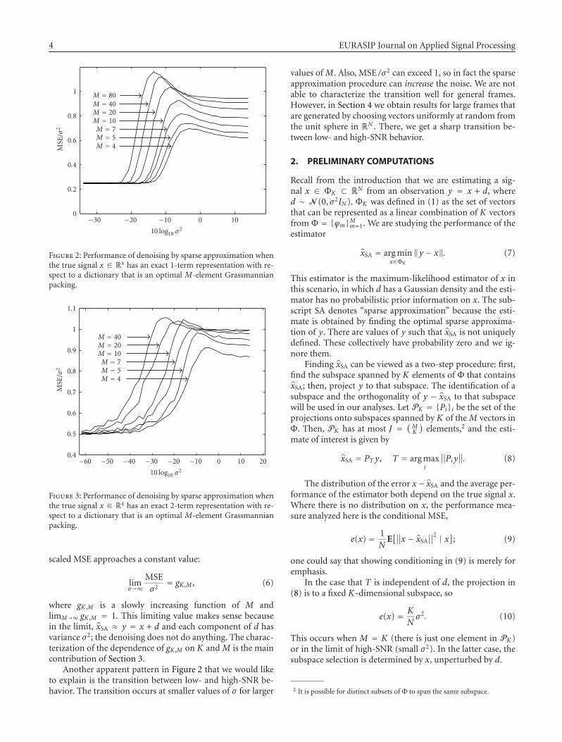
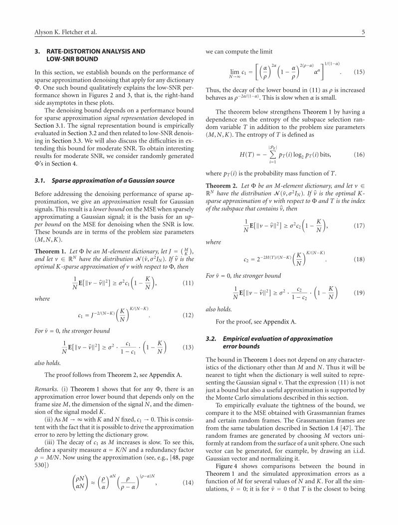
Figure 2 shows the MSE as a function of σ for several val-ues of M. Note that for visual clarity, MSE /σ2 is plotted, andall of the same properties are illustrated forK = 2 in Figure 3.For small values of σ , the MSE is (1/4)σ2. This is an exampleof the general statement that

MSE = K

Nσ2 for small σ , (5)

as described in detail in Section 2. For large values of σ , the


100−10−20−30

10 log10 σ2

0

0.2

0.4

0.6

0.8

1

MSE

/σ2

M = 80M = 40M = 20M = 10M = 7M = 5M = 4

Figure 2: Performance of denoising by sparse approximation whenthe true signal x ∈ R4 has an exact 1-term representation with re-spect to a dictionary that is an optimal M-element Grassmannianpacking.

20100−10−20−30−40−50−60

10 log10 σ2

0.4

0.5

0.6

0.7

0.8

0.9

1

1.1

MSE

/σ2

M = 40M = 20M = 10M = 7M = 5M = 4

Figure 3: Performance of denoising by sparse approximation whenthe true signal x ∈ R4 has an exact 2-term representation with re-spect to a dictionary that is an optimal M-element Grassmannianpacking.

scaled MSE approaches a constant value:

limσ→∞

MSEσ2

= gK ,M , (6)

where gK ,M is a slowly increasing function of M andlimM→∞ gK ,M = 1. This limiting value makes sense becausein the limit, xSA ≈ y = x + d and each component of d hasvariance σ2; the denoising does not do anything. The charac-terization of the dependence of gK ,M on K and M is the maincontribution of Section 3.

Another apparent pattern in Figure 2 that we would liketo explain is the transition between low- and high-SNR be-havior. The transition occurs at smaller values of σ for larger

values of M. Also, MSE /σ2 can exceed 1, so in fact the sparseapproximation procedure can increase the noise. We are notable to characterize the transition well for general frames.However, in Section 4 we obtain results for large frames thatare generated by choosing vectors uniformly at random fromthe unit sphere in RN . There, we get a sharp transition be-tween low- and high-SNR behavior.

2. PRELIMINARY COMPUTATIONS

Recall from the introduction that we are estimating a sig-nal x ∈ ΦK ⊂ RN from an observation y = x + d, whered ∼ N (0, σ2IN ). ΦK was defined in (1) as the set of vectorsthat can be represented as a linear combination of K vectorsfrom Φ = {ϕm}Mm=1. We are studying the performance of theestimator

xSA = arg minx∈ΦK

‖y − x‖. (7)

This estimator is the maximum-likelihood estimator of x inthis scenario, in which d has a Gaussian density and the esti-mator has no probabilistic prior information on x. The sub-script SA denotes “sparse approximation” because the esti-mate is obtained by finding the optimal sparse approxima-tion of y. There are values of y such that xSA is not uniquelydefined. These collectively have probability zero and we ig-nore them.

Finding xSA can be viewed as a two-step procedure: first,find the subspace spanned by K elements of Φ that containsxSA; then, project y to that subspace. The identification of asubspace and the orthogonality of y − xSA to that subspacewill be used in our analyses. Let PK = {Pi}i be the set of theprojections onto subspaces spanned by K of the M vectors inΦ. Then, PK has at most J = (

MK

)elements,2 and the esti-

mate of interest is given by

xSA = PT y, T = arg maxi

∥∥Pi y∥∥. (8)

The distribution of the error x− xSA and the average per-formance of the estimator both depend on the true signal x.Where there is no distribution on x, the performance mea-sure analyzed here is the conditional MSE,

e(x) = 1N

E[∥∥x − xSA

∥∥2 | x]; (9)

one could say that showing conditioning in (9) is merely foremphasis.

In the case that T is independent of d, the projection in(8) is to a fixed K-dimensional subspace, so

e(x) = K

Nσ2. (10)

This occurs when M = K (there is just one element in PK )or in the limit of high-SNR (small σ2). In the latter case, thesubspace selection is determined by x, unperturbed by d.

2 It is possible for distinct subsets of Φ to span the same subspace.


3. RATE-DISTORTION ANALYSIS ANDLOW-SNR BOUND

In this section, we establish bounds on the performance ofsparse approximation denoising that apply for any dictionaryΦ. One such bound qualitatively explains the low-SNR per-formance shown in Figures 2 and 3, that is, the right-handside asymptotes in these plots.

The denoising bound depends on a performance boundfor sparse approximation signal representation developed inSection 3.1. The signal representation bound is empiricallyevaluated in Section 3.2 and then related to low-SNR denois-ing in Section 3.3. We will also discuss the difficulties in ex-tending this bound for moderate SNR. To obtain interestingresults for moderate SNR, we consider randomly generatedΦ’s in Section 4.

3.1. Sparse approximation of a Gaussian source

Before addressing the denoising performance of sparse ap-proximation, we give an approximation result for Gaussiansignals. This result is a lower bound on the MSE when sparselyapproximating a Gaussian signal; it is the basis for an up-per bound on the MSE for denoising when the SNR is low.These bounds are in terms of the problem size parameters(M,N ,K).

Theorem 1. Let Φ be an M-element dictionary, let J = (MK

),

and let v ∈ RN have the distribution N (v, σ2IN ). If v is theoptimal K-sparse approximation of v with respect to Φ, then

1N

E[‖v − v‖2] ≥ σ2c1

(1− K

N

), (11)

where

c1 = J−2/(N−K)(K

N

)K/(N−K)

. (12)

For v = 0, the stronger bound

1N

E[‖v − v‖2] ≥ σ2 · c1

1− c1·(

1− K

N

)(13)

also holds.

The proof follows from Theorem 2, see Appendix A.

Remarks. (i) Theorem 1 shows that for any Φ, there is anapproximation error lower bound that depends only on theframe size M, the dimension of the signal N , and the dimen-sion of the signal model K .

(ii) As M →∞with K and N fixed, c1 → 0. This is consis-tent with the fact that it is possible to drive the approximationerror to zero by letting the dictionary grow.

(iii) The decay of c1 as M increases is slow. To see this,define a sparsity measure α = K/N and a redundancy factorρ = M/N . Now using the approximation (see, e.g., [48, page530]) (

ρNαN

)≈(ρ

α

)αN( ρ

ρ − α

)(ρ−α)N

, (14)

we can compute the limit

limN→∞

c1 =[(

α

ρ

)2α(1− α

ρ

)2(ρ−α)

αα]1/(1−α)

. (15)

Thus, the decay of the lower bound in (11) as ρ is increasedbehaves as ρ−2α/(1−α). This is slow when α is small.

The theorem below strengthens Theorem 1 by having adependence on the entropy of the subspace selection ran-dom variable T in addition to the problem size parameters(M,N ,K). The entropy of T is defined as

H(T) = −|PK |∑i=1

pT(i) log2 pT(i) bits, (16)

where pT(i) is the probability mass function of T .

Theorem 2. Let Φ be an M-element dictionary, and let v ∈RN have the distribution N (v, σ2IN ). If v is the optimal K-sparse approximation of v with respect to Φ and T is the indexof the subspace that contains v, then

1N

E[‖v − v‖2] ≥ σ2c2

(1− K

N

), (17)

where

c2 = 2−2H(T)/(N−K)(K

N

)K/(N−K)

. (18)

For v = 0, the stronger bound

1N

E[‖v − v‖2] ≥ σ2 · c2

1− c2·(

1− K

N

)(19)

also holds.

For the proof, see Appendix A.

3.2. Empirical evaluation of approximationerror bounds

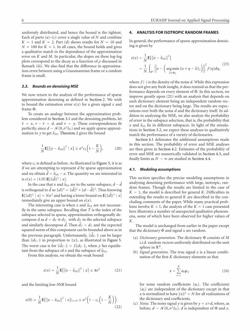
The bound in Theorem 1 does not depend on any character-istics of the dictionary other than M and N . Thus it will benearest to tight when the dictionary is well suited to repre-senting the Gaussian signal v. That the expression (11) is notjust a bound but also a useful approximation is supported bythe Monte Carlo simulations described in this section.

To empirically evaluate the tightness of the bound, wecompare it to the MSE obtained with Grassmannian framesand certain random frames. The Grassmannian frames arefrom the same tabulation described in Section 1.4 [47]. Therandom frames are generated by choosing M vectors uni-formly at random from the surface of a unit sphere. One suchvector can be generated, for example, by drawing an i.i.d.Gaussian vector and normalizing it.

Figure 4 shows comparisons between the bound inTheorem 1 and the simulated approximation errors as afunction of M for several values of N and K . For all the sim-ulations, v = 0; it is for v = 0 that T is the closest to being


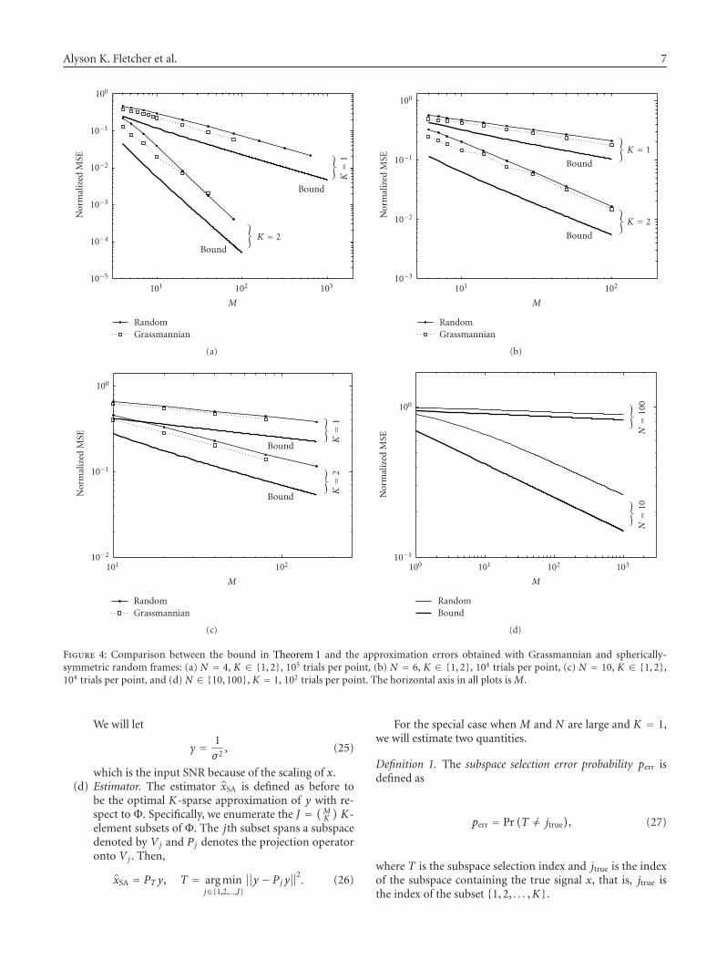
uniformly distributed, and hence the bound is the tightest.Each of parts (a)–(c) cover a single value of N and combineK = 1 and K = 2. Part (d) shows results for N = 10 andN = 100 for K = 1. In all cases, the bound holds and givesa qualitative match in the dependence of the approximationerror on K and M. In particular, the slopes on these log-logplots correspond to the decay as a function of ρ discussed inRemark (iii). We also find that the difference in approxima-tion error between using a Grassmannian frame or a randomframe is small.

3.3. Bounds on denoising MSE

We now return to the analysis of the performance of sparseapproximation denoising as defined in Section 2. We wishto bound the estimation error e(x) for a given signal x andframe Φ.

To create an analogy between the approximation prob-lem considered in Section 3.1 and the denoising problem, letv = x, v − v = d, and v = y. These correspondences fitperfectly, since d ∼ N (0, σ2IN ) and we apply sparse approxi-mation to y to get xSA. Theorem 2 gives the bound

1N

E[∥∥y − xSA

∥∥2 | x] ≥ σ2c2

(1− K

N

), (20)

where c2 is defined as before. As illustrated in Figure 5, it is asif we are attempting to represent d by sparse approximation

and we obtain d = xSA − x. The quantity we are interested in

is e(x) = (1/N)E[‖d‖2 | x].In the case that x and xSA are in the same subspace, d− d

is orthogonal to d so ‖d‖2 = ‖d‖2 +‖d− d‖2. Thus knowing

E[‖d‖2 | x] = Nσ2 and having a lower bound on E[‖d‖2 | x]immediately give an upper bound on e(x).

The interesting case is when x and xSA are not necessar-ily in the same subspace. Recalling that T is the index of thesubspace selected in sparse, approximation orthogonally de-compose d as d = dT ⊕ dT⊥ with dT in the selected subspace

and similarly decompose d. Then dT = dT and the expectedsquared norm of this component can be bounded above as in

the previous paragraph. Unfortunately, ‖dT⊥‖ can be largerthan ‖dT⊥‖ in proportion to ‖x‖, as illustrated in Figure 5.

The worst case is for ‖dT⊥‖ = 2‖dT⊥‖, when y lies equidis-tant from the subspace of x and the subspace of xSA.

From this analysis, we obtain the weak bound

e(x) = 1N

E[∥∥x − xSA

∥∥2 | x] ≤ 4σ2 (21)

and the limiting low-SNR bound

e(0) = 1N

E[∥∥x − xSA

∥∥2 | x]|x=0 ≤ σ2(

1− c2

(1− K

N

)).

(22)

4. ANALYSIS FOR ISOTROPIC RANDOM FRAMES

In general, the performance of sparse approximation denois-ing is given by

e(x) = 1N

E[∥∥x − xSA

∥∥2]

= 1N

∫RN

∥∥∥∥x −(

arg minx∈ΦK

‖x + η − x‖2

)∥∥∥∥2

f (η)dη,(23)

where f (·) is the density of the noise d. While this expressiondoes not give any fresh insight, it does remind us that the per-formance depends on every element of Φ. In this section, weimprove greatly upon (21) with an analysis that depends oneach dictionary element being an independent random vec-tor and on the dictionary being large. The results are expec-tations over both the noise d and the dictionary itself. In ad-dition to analyzing the MSE, we also analyze the probabilityof error in the subspace selection, that is, the probability thatx and xSA lie in different subspaces. In light of the simula-tions in Section 3.2, we expect these analyses to qualitativelymatch the performance of a variety of dictionaries.

Section 4.1 delineates the additional assumptions madein this section. The probability of error and MSE analysesare then given in Section 4.2. Estimates of the probability oferror and MSE are numerically validated in Section 4.3, andfinally limits as N →∞ are studied in Section 4.4.

4.1. Modeling assumptions

This section specifies the precise modeling assumptions inanalyzing denoising performance with large, isotropic, ran-dom frames. Though the results are limited to the case ofK = 1, the model is described for general K . Difficulties inextending the results to general K are described in the con-cluding comments of the paper. While many practical prob-lems involve K > 1, the analysis of the K = 1 case presentedhere illustrates a number of unexpected qualitative phenom-ena, some of which have been observed for higher values ofK .

The model is unchanged from earlier in the paper exceptthat the dictionary Φ and signal x are random.

(a) Dictionary generation. The dictionary Φ consists of Mi.i.d. random vectors uniformly distributed on the unitsphere in RN .

(b) Signal generation. The true signal x is a linear combi-nation of the first K dictionary elements so that

x =K∑i=1

αiϕi, (24)

for some random coefficients {αi}. The coefficients{αi} are independent of the dictionary except in thatx is normalized to have ‖x‖2 = N for all realizations ofthe dictionary and coefficients.

(c) Noise. The noisy signal y is given by y = x+d, where, asbefore, d ∼ N (0, σ2IN ). d is independent of Φ and x.


103102101

M

10−5

10−4

10−3

10−2

10−1

100

Nor

mal

ized

MSE

RandomGrassmannian

Bound

Bound

}

K=

1

}K = 2

(a)

102101

M

10−3

10−2

10−1

100

Nor

mal

ized

MSE

RandomGrassmannian

Bound

Bound

}K = 1

}K = 2

(b)

102101

M

10−2

10−1

100

Nor

mal

ized

MSE

RandomGrassmannian

Bound

Bound

}

K=

1

}

K=

2

(c)

103102101100

M

10−1

100

Nor

mal

ized

MSE

RandomBound

}

N=

100

}

N=

10(d)

Figure 4: Comparison between the bound in Theorem 1 and the approximation errors obtained with Grassmannian and spherically-symmetric random frames: (a) N = 4, K ∈ {1, 2}, 105 trials per point, (b) N = 6, K ∈ {1, 2}, 104 trials per point, (c) N = 10, K ∈ {1, 2},104 trials per point, and (d) N ∈ {10, 100}, K = 1, 102 trials per point. The horizontal axis in all plots is M.

We will let

γ = 1σ2

, (25)

which is the input SNR because of the scaling of x.(d) Estimator. The estimator xSA is defined as before to

be the optimal K-sparse approximation of y with re-spect to Φ. Specifically, we enumerate the J = (MK ) K-element subsets of Φ. The jth subset spans a subspacedenoted by Vj and Pj denotes the projection operatoronto Vj . Then,

xSA = PT y, T = arg minj∈{1,2,...,J}

∥∥y − Pj y∥∥2. (26)

For the special case when M and N are large and K = 1,we will estimate two quantities.

Definition 1. The subspace selection error probability perr isdefined as

perr = Pr(T �= jtrue

), (27)

where T is the subspace selection index and jtrue is the indexof the subspace containing the true signal x, that is, jtrue isthe index of the subset {1, 2, . . . ,K}.


0

x

xSA

y

d − d

d

d

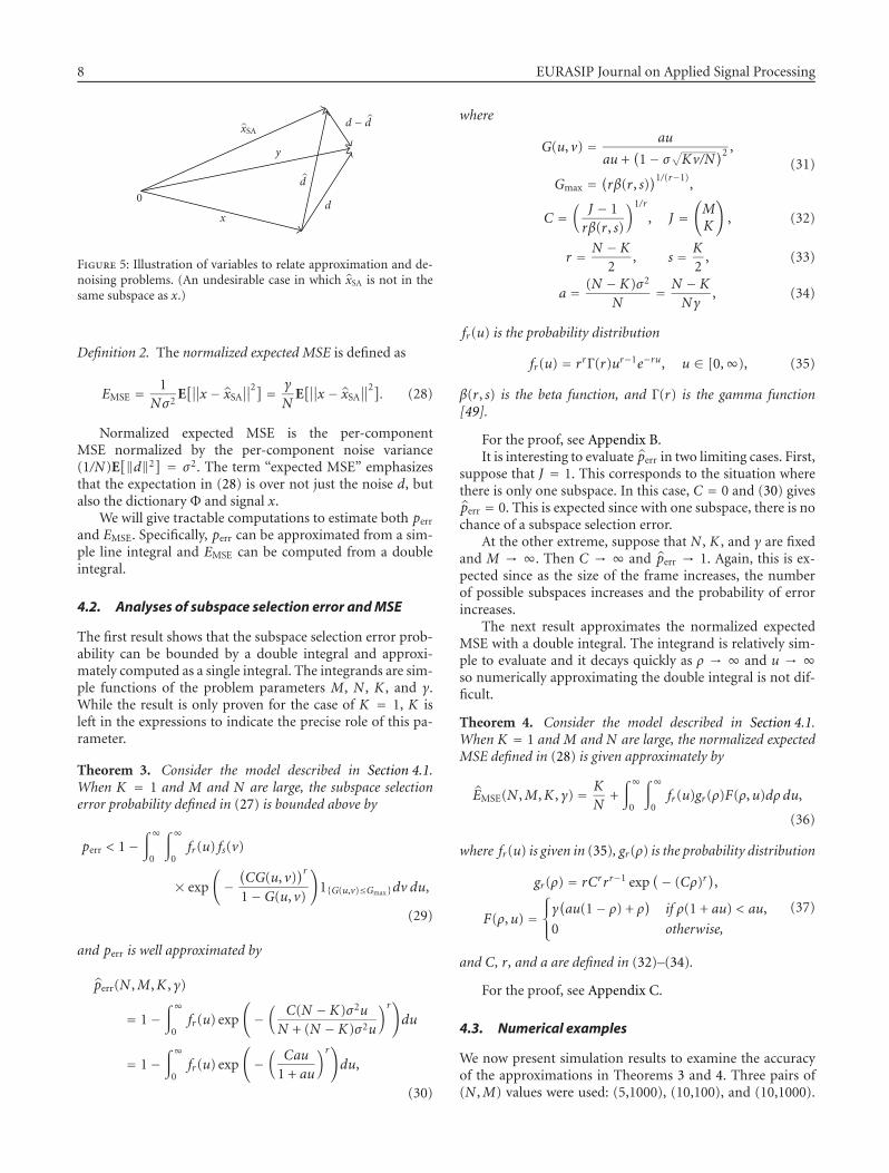
Figure 5: Illustration of variables to relate approximation and de-noising problems. (An undesirable case in which xSA is not in thesame subspace as x.)

Definition 2. The normalized expected MSE is defined as

EMSE = 1Nσ2

E[∥∥x − xSA

∥∥2] = γ

NE[∥∥x − xSA

∥∥2]. (28)

Normalized expected MSE is the per-componentMSE normalized by the per-component noise variance(1/N)E

[‖d‖2] = σ2. The term “expected MSE” emphasizes

that the expectation in (28) is over not just the noise d, butalso the dictionary Φ and signal x.

We will give tractable computations to estimate both perr

and EMSE. Specifically, perr can be approximated from a sim-ple line integral and EMSE can be computed from a doubleintegral.

4.2. Analyses of subspace selection error and MSE

The first result shows that the subspace selection error prob-ability can be bounded by a double integral and approxi-mately computed as a single integral. The integrands are sim-ple functions of the problem parameters M, N , K , and γ.While the result is only proven for the case of K = 1, K isleft in the expressions to indicate the precise role of this pa-rameter.

Theorem 3. Consider the model described in Section 4.1.When K = 1 and M and N are large, the subspace selectionerror probability defined in (27) is bounded above by

perr < 1−∫∞

0

∫∞0

fr(u) fs(v)

× exp

(−(CG(u, v)

)r1−G(u, v)

)1{G(u,v)≤Gmax}dv du,

(29)

and perr is well approximated by

perr(N ,M,K , γ)

= 1−∫∞

0fr(u) exp

(−(

C(N − K)σ2u

N + (N − K)σ2u

)r)du

= 1−∫∞

0fr(u) exp

(−(

Cau

1 + au

)r)du,

(30)

where

G(u, v) = au

au +(1− σ

√Kv/N

)2 ,

Gmax =(rβ(r, s)

)1/(r−1),

(31)

C =(

J − 1rβ(r, s)

)1/r

, J =(MK

), (32)

r = N − K

2, s = K

2, (33)

a = (N − K)σ2

N= N − K

Nγ, (34)

fr(u) is the probability distribution

fr(u) = rrΓ(r)ur−1e−ru, u ∈ [0,∞), (35)

β(r, s) is the beta function, and Γ(r) is the gamma function[49].

For the proof, see Appendix B.It is interesting to evaluate perr in two limiting cases. First,

suppose that J = 1. This corresponds to the situation wherethere is only one subspace. In this case, C = 0 and (30) givesperr = 0. This is expected since with one subspace, there is nochance of a subspace selection error.

At the other extreme, suppose that N , K , and γ are fixedand M → ∞. Then C → ∞ and perr → 1. Again, this is ex-pected since as the size of the frame increases, the numberof possible subspaces increases and the probability of errorincreases.

The next result approximates the normalized expectedMSE with a double integral. The integrand is relatively sim-ple to evaluate and it decays quickly as ρ → ∞ and u → ∞so numerically approximating the double integral is not dif-ficult.

Theorem 4. Consider the model described in Section 4.1.When K = 1 and M and N are large, the normalized expectedMSE defined in (28) is given approximately by

EMSE(N ,M,K , γ) = K

N+∫∞

0

∫∞0

fr(u)gr(ρ)F(ρ,u)dρ du,

(36)

where fr(u) is given in (35), gr(ρ) is the probability distribution

gr(ρ) = rCrrr−1 exp(− (Cρ)r

),

F(ρ,u) =⎧⎨⎩γ(au(1− ρ) + ρ

)if ρ(1 + au) < au,

0 otherwise,

(37)

and C, r, and a are defined in (32)–(34).

For the proof, see Appendix C.

4.3. Numerical examples

We now present simulation results to examine the accuracyof the approximations in Theorems 3 and 4. Three pairs of(N ,M) values were used: (5,1000), (10,100), and (10,1000).


35302520151050−5−10

SNR (dB)

−5

−4

−3

−2

−1

0

log 10

(per

r.)

SimulatedTheoretical

(10, 100) (10, 1000) (5, 1000)

(a)

35302520151050−5−10

SNR (dB)

0

0.2

0.4

0.6

0.8

1

EM

SE

SimulatedTheoretical

(10, 100) (10, 1000) (5, 1000)

(b)

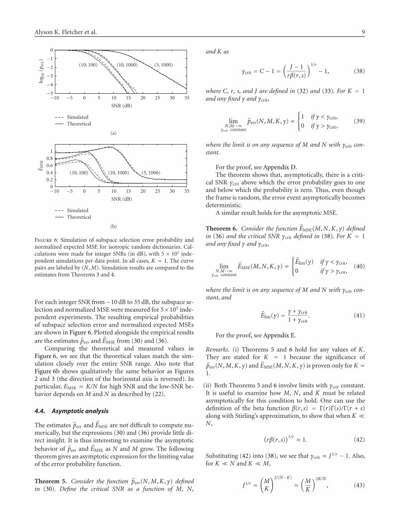
Figure 6: Simulation of subspace selection error probability andnormalized expected MSE for isotropic random dictionaries. Cal-culations were made for integer SNRs (in dB), with 5 × 105 inde-pendent simulations per data point. In all cases, K = 1. The curvepairs are labeled by (N ,M). Simulation results are compared to theestimates from Theorems 3 and 4.

For each integer SNR from−10 dB to 35 dB, the subspace se-lection and normalized MSE were measured for 5×105 inde-pendent experiments. The resulting empirical probabilitiesof subspace selection error and normalized expected MSEsare shown in Figure 6. Plotted alongside the empirical resultsare the estimates perr and EMSE from (30) and (36).

Comparing the theoretical and measured values inFigure 6, we see that the theoretical values match the sim-ulation closely over the entire SNR range. Also note thatFigure 6b shows qualitatively the same behavior as Figures2 and 3 (the direction of the horizontal axis is reversed). Inparticular, EMSE ≈ K/N for high SNR and the low-SNR be-havior depends on M and N as described by (22).

4.4. Asymptotic analysis

The estimates perr and EMSE are not difficult to compute nu-merically, but the expressions (30) and (36) provide little di-rect insight. It is thus interesting to examine the asymptoticbehavior of perr and EMSE as N and M grow. The followingtheorem gives an asymptotic expression for the limiting valueof the error probability function.

Theorem 5. Consider the function perr(N ,M,K , γ) definedin (30). Define the critical SNR as a function of M, N ,

and K as

γcrit = C − 1 =(

J − 1rβ(r, s)

)1/r

− 1, (38)

where C, r, s, and J are defined in (32) and (33). For K = 1and any fixed γ and γcrit,

limN ,M→∞

γcrit constant

perr(N ,M,K , γ) =⎧⎨⎩1 if γ < γcrit,

0 if γ > γcrit,(39)

where the limit is on any sequence of M and N with γcrit con-stant.

For the proof, see Appendix D.The theorem shows that, asymptotically, there is a criti-

cal SNR γcrit above which the error probability goes to oneand below which the probability is zero. Thus, even thoughthe frame is random, the error event asymptotically becomesdeterministic.

A similar result holds for the asymptotic MSE.

Theorem 6. Consider the function EMSE(M,N ,K , γ) definedin (36) and the critical SNR γcrit defined in (38). For K = 1and any fixed γ and γcrit,

limN ,M→∞

γcrit constant

EMSE(M,N ,K , γ) =⎧⎨⎩Elim(γ) if γ < γcrit,

0 if γ > γcrit,(40)

where the limit is on any sequence of M and N with γcrit con-stant, and

Elim(γ) = γ + γcrit

1 + γcrit. (41)

For the proof, see Appendix E.

Remarks. (i) Theorems 5 and 6 hold for any values of K .They are stated for K = 1 because the significance ofperr(N ,M,K , γ) and EMSE(M,N ,K , γ) is proven only for K =1.

(ii) Both Theorems 5 and 6 involve limits with γcrit constant.It is useful to examine how M, N , and K must be relatedasymptotically for this condition to hold. One can use thedefinition of the beta function β(r, s) = Γ(r)Γ(s)/Γ(r + s)along with Stirling’s approximation, to show that when K �N ,

(rβ(r, s)

)1/r ≈ 1. (42)

Substituting (42) into (38), we see that γcrit ≈ J1/r − 1. Also,for K � N and K �M,

J1/r =(MK

)2/(N−K)

≈(M

K

)2K/N

, (43)


10110010−110−2

SNR

0

0.2

0.4

0.6

0.8

1

1.2

1.4

Nor

mal

ized

MSE

γcrit. = 2

γcrit. = 1

γcrit. = 0.5

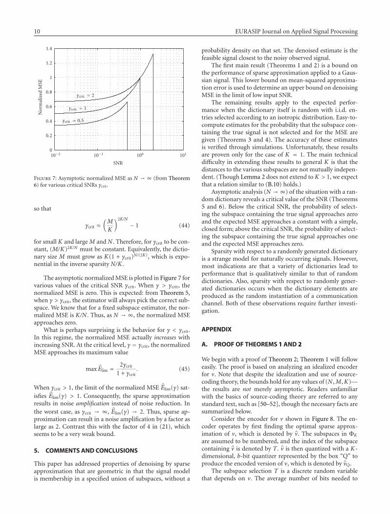
Figure 7: Asymptotic normalized MSE as N → ∞ (from Theorem6) for various critical SNRs γcrit.

so that

γcrit ≈(M

K

)2K/N

− 1 (44)

for small K and large M and N . Therefore, for γcrit to be con-stant, (M/K)2K/N must be constant. Equivalently, the dictio-nary size M must grow as K(1 + γcrit)N/(2K), which is expo-nential in the inverse sparsity N/K .

The asymptotic normalized MSE is plotted in Figure 7 forvarious values of the critical SNR γcrit. When γ > γcrit, thenormalized MSE is zero. This is expected: from Theorem 5,when γ > γcrit, the estimator will always pick the correct sub-space. We know that for a fixed subspace estimator, the nor-malized MSE is K/N . Thus, as N → ∞, the normalized MSEapproaches zero.

What is perhaps surprising is the behavior for γ < γcrit.In this regime, the normalized MSE actually increases withincreasing SNR. At the critical level, γ = γcrit, the normalizedMSE approaches its maximum value

max Elim = 2γcrit

1 + γcrit. (45)

When γcrit > 1, the limit of the normalized MSE Elim(γ) sat-isfies Elim(γ) > 1. Consequently, the sparse approximationresults in noise amplification instead of noise reduction. Inthe worst case, as γcrit → ∞, Elim(γ) → 2. Thus, sparse ap-proximation can result in a noise amplification by a factor aslarge as 2. Contrast this with the factor of 4 in (21), whichseems to be a very weak bound.

5. COMMENTS AND CONCLUSIONS

This paper has addressed properties of denoising by sparseapproximation that are geometric in that the signal modelis membership in a specified union of subspaces, without a

probability density on that set. The denoised estimate is thefeasible signal closest to the noisy observed signal.

The first main result (Theorems 1 and 2) is a bound onthe performance of sparse approximation applied to a Gaus-sian signal. This lower bound on mean-squared approxima-tion error is used to determine an upper bound on denoisingMSE in the limit of low input SNR.

The remaining results apply to the expected perfor-mance when the dictionary itself is random with i.i.d. en-tries selected according to an isotropic distribution. Easy-to-compute estimates for the probability that the subspace con-taining the true signal is not selected and for the MSE aregiven (Theorems 3 and 4). The accuracy of these estimatesis verified through simulations. Unfortunately, these resultsare proven only for the case of K = 1. The main technicaldifficulty in extending these results to general K is that thedistances to the various subspaces are not mutually indepen-dent. (Though Lemma 2 does not extend to K > 1, we expectthat a relation similar to (B.10) holds.)

Asymptotic analysis (N →∞) of the situation with a ran-dom dictionary reveals a critical value of the SNR (Theorems5 and 6). Below the critical SNR, the probability of select-ing the subspace containing the true signal approaches zeroand the expected MSE approaches a constant with a simple,closed form; above the critical SNR, the probability of select-ing the subspace containing the true signal approaches oneand the expected MSE approaches zero.

Sparsity with respect to a randomly generated dictionaryis a strange model for naturally occurring signals. However,most indications are that a variety of dictionaries lead toperformance that is qualitatively similar to that of randomdictionaries. Also, sparsity with respect to randomly gener-ated dictionaries occurs when the dictionary elements areproduced as the random instantiation of a communicationchannel. Both of these observations require further investi-gation.

APPENDIX

A. PROOF OF THEOREMS 1 AND 2

We begin with a proof of Theorem 2; Theorem 1 will followeasily. The proof is based on analyzing an idealized encoderfor v. Note that despite the idealization and use of source-coding theory, the bounds hold for any values of (N ,M,K)—the results are not merely asymptotic. Readers unfamiliarwith the basics of source-coding theory are referred to anystandard text, such as [50–52], though the necessary facts aresummarized below.

Consider the encoder for v shown in Figure 8. The en-coder operates by first finding the optimal sparse approx-imation of v, which is denoted by v. The subspaces in ΦK

are assumed to be numbered, and the index of the subspacecontaining v is denoted by T . v is then quantized with a K-dimensional, b-bit quantizer represented by the box “Q” toproduce the encoded version of v, which is denoted by vQ.

The subspace selection T is a discrete random variablethat depends on v. The average number of bits needed to


v

H(T) bits b bits

SA

v

TQ vQ

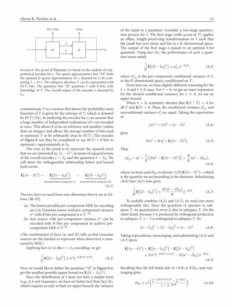
Figure 8: The proof of Theorem 2 is based on the analysis of a hy-pothetical encoder for v. The sparse approximation box “SA” findsthe optimal K-sparse approximation of v, denoted by v, by com-puting v = PTv. The subspace selection T can be represented withH(T) bits. The quantizer box “Q” quantizes v with b bits, withknowledge of T . The overall output of the encoder is denoted byvQ.

communicate T to a receiver that knows the probability massfunction of T is given by the entropy of T , which is denotedby H(T) [51]. In analyzing the encoder for v, we assume thata large number of independent realizations of v are encodedat once. This allows b to be an arbitrary real number (ratherthan an integer) and allows the average number of bits usedto represent T to be arbitrarily close to H(T). The encoderof Figure 8 can thus be considered to use H(T) + b bits torepresent v approximately as vQ.

The crux of the proof is to represent the squared errorthat we are interested in, ‖v− v‖2, in terms of squared errorsof the overall encoder v �→ vQ and the quantizer v �→ vQ. Wewill show the orthogonality relationship below and boundboth terms:

E[‖v − v‖2] = E

[∥∥v − vQ∥∥2]︸︷︷︸

bounded below using fact (a)

− E[‖v − vQ‖2]︸︷︷︸

bounded above using fact (b)

.

(A.1)

The two facts we need from rate-distortion theory are as fol-lows [50–52].

(a) The lowest possible per-component MSE for encodingan i.i.d. Gaussian source with per-component varianceσ2 with R bits per component is σ22−2R.

(b) Any source with per-component variance σ2 can beencoded with R bits per component to achieve per-component MSE σ22−2R.

(The combination of facts (a) and (b) tells us that Gaussiansources are the hardest to represent when distortion is mea-sured by MSE.)

Applying fact (a) to the v �→ vQ encoding, we get

1N

E[∥∥v − vQ

∥∥2] ≥ σ22−2(H(T)+b)/N . (A.2)

Now we would like to define the quantizer “Q” in Figure 8 toget the smallest possible upper bound on E[‖v − vQ‖2].

Since the distribution of v does not have a simple form(e.g., it is not Gaussian), we have no better tool than fact (b),which requires us only to find (or upper bound) the variance

of the input to a quantizer. Consider a two-stage quantiza-tion process for v. The first stage (with access to T) appliesan affine, length-preserving transformation to v such thatthe result has zero mean and lies in a K-dimensional space.The output of the first stage is passed to an optimal b-bitquantizer. Using fact (b), the performance of such a quan-tizer must satisfy

1K

E[∥∥v − vQ

∥∥2] ≤ σ2v|T2−2b/K , (A.3)

where σ2v|T is the per-component conditional variance of v,

in the K-dimensional space, conditioned on T .From here on, we have slightly different reasoning for the

v = 0 and v �= 0 cases. For v = 0, we get an exact expressionfor the desired conditional variance; for v �= 0, we use anupper bound.

When v = 0, symmetry dictates that E[v | T] = 0 forall T and E[v] = 0. Thus, the conditional variance σ2

v|T andunconditional variance σ2

v are equal. Taking the expectationof

‖v‖2 = ‖v‖2 + ‖v − v‖2 (A.4)

gives

Nσ2 = Kσ2v + E

[‖v − v‖2]. (A.5)

Thus

σ2v|T = σ2

v =1K

(Nσ2 − E

[‖v − v‖2]) = N

K

(σ2 −DSA

),

(A.6)

where we have used DSA to denote (1/N)E[‖v− v‖2]—whichis the quantity we are bounding in the theorem. Substituting(A.6) into (A.3) now gives

1K

E[∥∥v − vQ

∥∥2] ≤ N(σ2 −DSA

)K

2−2b/K . (A.7)

To usefully combine (A.2) and (A.7), we need one moreorthogonality fact. Since the quantizer Q operates in sub-space T , its quantization error is also in subspace T . On theother hand, because v is produced by orthogonal projectionto subspace T , v − v is orthogonal to subspace T . So

∥∥v − vQ∥∥2 = ∥∥v − vQ

∥∥2+ ‖v − v‖2. (A.8)

Taking expectations, rearranging, and substituting (A.2) and(A.7) gives

E[‖v − v‖2] = E

[∥∥v − vQ∥∥2]− E

[∥∥v − vQ∥∥2]

≥ Nσ22−2(H(T)+b)/N −N(σ2 −DSA

)2−2b/K .

(A.9)

Recalling that the left-hand side of (A.9) is NDSA and rear-ranging gives

DSA ≥ σ2(

2−2(H(T)+b)/N − 2−2b/K

1− 2−2b/K

). (A.10)


Since this bound must be true for all b ≥ 0, one can max-imize with respect to b to obtain the strongest bound. Thismaximization is messy; however, maximizing the numeratoris easier and gives almost as strong a bound. The numeratoris maximized when

b = K

N − K

(H(T) +

N

2log2

N

K

), (A.11)

and substituting this value of b in (A.10) gives

DSA ≥ σ2 · 2−2H(T)/(N−K)(1− (K/N))(K/N)K/(N−K)

1− 2−2H(T)/(N−K)(K/N)N/(N−K).

(A.12)

We have now completed the proof of Theorem 2 for v = 0.For v �= 0, there is no simple expression for σ2

v|T that doesnot depend on the geometry of the dictionary, such as (A.6),to use in (A.3). Instead, use

σ2v|T ≤ σ2

v ≤N

Kσ2, (A.13)

where the first inequality holds because conditioning cannotincrease variance and the second follows from the fact thatthe orthogonal projection of v cannot increase its variance,even if the choice of projection depends on v. Now followingthe same steps as for the v = 0 case yields

DSA ≥ σ2(2−2(H(T)+b)/N − 2−2b/K) (A.14)

in place of (A.10). The bound is optimized over b to obtain

DSA ≥ σ2 · 2−2H(T)/(N−K)(

1−(K

N

))(K

N

)K/(N−K)

.

(A.15)

The proof of Theorem 1 now follows directly: since T isa discrete random variable that can take at most J values,H(T) ≤ log2 J .

B. PROOF OF THEOREM 3

Using the notation of Section 4.1, let Vj , j = 1, 2, . . . , J , bethe subspaces spanned by the J possible K-element subsetsof the dictionary Φ. Let Pj be the projection operator ontoVj , and let T be index of the subspace closest to y. Let jtrue

be the index of the subspace containing the true signal x, sothat the probability of error is

perr = Pr(T �= jtrue

). (B.1)

For each j, let x j = Pj y, so that the estimator xSA in (26)can be rewritten as xSA = xT . Also, define random variables

ρj =∥∥y − x j

∥∥2

‖y‖2, j = 1, 2, . . . , J , (B.2)

to represent the normalized distances between y and the Vj ’s.Henceforth, the ρj ’s will be called angles, since ρj = sin2 θj ,where θj is the angle between y and Vj . The angles are welldefined since ‖y‖2 > 0 with probability one.

Lemma 1. For all j �= jtrue, the angle ρj is independent of xand d.

Proof. Given a subspace V and vector y, define the function

R(y,V) =∥∥y − PV y

∥∥2

‖y‖2, (B.3)

where PV is the projection operator onto the subspace y.Thus, R(y,V) is the angle between y and V . With this no-tation, ρj = R(y,Vj). Since ρj is a deterministic function ofy and Vj and y = x+d, to show ρj is independent of x and d,it suffices to prove that ρj is independent of y. Equivalently,we need to show that for any function G(ρ) and vectors y0

and y1,

E[G(ρj) | y = y0

] = E[G(ρj) | y = y1

]. (B.4)

This property can be proven with the following symmetryargument. Let U be any orthogonal transformation. Since Uis orthogonal, PUV (Uy) = UPV y for all subspaces V andvectors y. Combining this with the fact that ‖Uv‖ = ‖v‖ forall v, we see that

R(Uy,UV) =∥∥Uy − PUV (Uy)

∥∥2

‖Uy‖2=∥∥U(y − PV (y)

)∥∥2

‖Uy‖2

=∥∥y − PV (y)

∥∥2

‖y‖2= R(y,V).

(B.5)

Also, for any scalar α > 0, it can be verified that R(αy,V) =R(y,V).

Now, let y0 and y1 be any two possible nonzero values forthe vector y. Then, there exist an orthogonal transformationU and scalar α > 0 such that y1 = αUy0. Since j �= jtrue andK = 1, the subspace Vj is spanned by vectors ϕi, independentof the vector y. Therefore,

E[G(ρj)| y= y1

] =E[G(R(y1,Vj

))] = E[G(R(αUy0,Vj

))]= E

[G(R(Uy0,Vj

))].

(B.6)

Now since the elements of Φ are distributed uniformly onthe unit sphere, the subspace UVj is identically distributedto Vj . Combining this with (B.5) and (B.6),

E[G(ρj) | y = y1

]= E

[G(R(Uy0,Vj

))] = E[G(R(Uy0,UVj

))]= E

[G(R(y0,Vj

))] = E[G(ρj) | y = y0

],

(B.7)

and this completes the proof.

Lemma 2. The random angles ρj , j �= jtrue, are i.i.d., each witha probability density function given by the beta distribution

pρ(ρ) = 1β(r, s)

ρr−1(1− ρ)s−1, 0 ≤ ρ ≤ 1, (B.8)

where r = (N − K)/2 and s = K/2 as defined in (33).


Proof. Since K = 1, each of the subspaces Vj for j �= jtrue isspanned by a single, unique vector in Φ. Since the vectors inΦ are independent and the random variables ρj are the anglesbetween y and the spaces Vj , the angles are independent.

Now consider a single angle ρj for j �= jtrue. The angle ρjis the angle between y and a random subspace Vj . Since thedistribution of the random vectors defining Vj is sphericallysymmetric and ρj is independent of y, ρj is identically dis-tributed to the angle between any fixed subspaceV and a ran-dom vector z uniformly distributed on the unit sphere. Oneway to create such a random vector z is to take z = w/‖w‖,where w ∼ N (0, IN ). Let w1,w2, . . . ,wK be the componentsof w in V , and let wK+1,wK+2, . . . ,wN be the components inthe orthogonal complement to V . If we define

X =K∑i=1

w2i , Y =

N∑i=K+1

w2i , (B.9)

then the angle between z and V is ρ = Y/(X+Y). Since X andY are the sums of K and N − K i.i.d. squared Gaussian ran-dom variables, they are Chi-squared random variables withK and N − K degrees of freedom, respectively [53]. Now,a well-known property of Chi-squared random variables isthat if X and Y are Chi-squared random variables with mand n degrees of freedom, Y/(X + Y) will have the beta dis-tribution with parameters m/2 and n/2. Thus, ρ = Y/(X +Y)has the beta distribution, with parameters r and s defined in(33). The probability density function for the beta distribu-tion is given in (B.8).

Lemma 3. Let ρmin = min j �= jtrue ρj . Then ρmin is independentof x and d and has the approximate distribution

Pr(ρmin > ε

) ≈ exp(− (Cε)r

)(B.10)

for small ε, where C is given in (32). More precisely,

Pr(ρmin>ε

)<exp

(−(Cε)r(1−ε)s−1) for all ε ∈ (0, 1),

Pr(ρmin>ε

)>exp

(− (Cε)r

(1−ε)

)for 0<ε

(rβ(r, s)

)1/(r−1).

(B.11)

Proof. Since Lemma 1 shows that each ρj is independent of xand d, it follows that ρmin is independent of x and d as well.Also, for any j �= jtrue, by bounding the integrand of

Pr(ρj < ε

) = 1β(r, s)

∫ ε0ρr−1(1− ρ)s−1dρ (B.12)

from above and below, we obtain the bounds

(1− ε)s−1

β(r, s)

∫ ε0ρr−1dρ < Pr

(ρj < ε

)<

1β(r, s)

∫ ε0ρr−1dρ,

(B.13)

which simplify to

(1− ε)s−1εr

rβ(r, s)< Pr

(ρj < ε

)<

εr

rβ(r, s). (B.14)

Now, there are J − 1 subspaces Vj where j �= jtrue,and by Lemma 2, the ρj ’s are mutually independent. Con-sequently, if we apply the upper bound of (B.14) and 1− δ >exp(−δ/(1 − δ)) for δ ∈ (0, 1), with δ = εr /(rβ(r, s)), weobtain

Pr(ρmin > ε

)=

∏j �= jtrue

Pr(ρj > ε

)>(

1− εr

rβ(r, s)

)J−1

> exp(− εr(J − 1)

rβ(r, s)(1− δ)

)for 0 < ε < (rβ(r, s))1/r ,

> exp(− εr(J−1)rβ(r, s)(1−ε)

)for 0 < ε <

(rβ(r, s)

)1/(r−1).

(B.15)

Similarly, using the lower bound of (B.14), we obtain

Pr(ρmin > ε

) = ∏j �= jtrue

Pr(ρj > ε

)<(

1− (1− ε)s−1εr

rβ(r, s)

)J−1

< exp(− (1− ε)s−1εr(J − 1)

rβ(r, s)

).

(B.16)

Proof of Theorem 3. Let Vtrue be the “correct” subspace, thatis, Vtrue = Vj for j = jtrue. Let Dtrue be the squared distancefrom y to Vtrue, and let Dmin be the minimum of the squareddistances from y to the “incorrect” subspaces Vj , j �= jtrue.Since the estimator selects the closest subspace, there is anerror if and only if Dmin ≤ Dtrue. Thus,

perr = Pr(Dmin ≤ Dtrue

). (B.17)

To estimate this quantity, we will approximate the probabilitydistributions of Dmin and Dtrue.

First consider Dtrue. Write the noise vector d as d = d0 +d1, where d0 is the component in Vtrue and d1 is in V⊥

true. LetD0 = ‖d0‖2 and D1 = ‖d1‖2. Since y = x + d and x ∈ Vtrue,the squared distance from y to Vtrue is D1. Thus,

Dtrue = D1. (B.18)

Now consider Dmin. For any j, x j is the projection of yonto Vj . Thus, the squared distance from y to any space Vj

is ‖y − x j‖2 = ρj‖y‖2. Hence, the minimum of the squareddistances from y to the spaces Vj , j �= jtrue, is

Dmin = ρmin‖y‖2. (B.19)

We will bound and approximate ‖y‖2 to obtain the boundand approximation of the theorem. Notice that y = x + d =x+d0 +d1, where x+d0 ∈ Vtrue and d1 ∈ V⊥

true. Using this or-thogonality and the triangle inequality, we obtain the bound

‖y‖2 = ∥∥x + d0∥∥2

+∥∥d1

∥∥2 ≥ (‖x‖ − ∥∥d0∥∥)2

+∥∥d1

∥∥2

=(√

N −√D0

)2+ D1.

(B.20)


For an accurate approximation, note that since d0 is thecomponent of d in the K-dimensional space Vtrue, we haveD0 � N unless the SNR is very low. Thus,

‖y‖2 ≈ N + D1. (B.21)

Combining (B.17), (B.18), and (B.19) gives

perr = Pr(Dmin ≤ Dtrue

) = Pr(ρmin‖y‖2 ≤ D1

)

= Pr

(ρmin ≤ D1

‖y‖2

).

(B.22)

Note that by Lemma 3, ρmin is independent of x and d. There-fore, ρmin is independent of D0 and D1. We can now obtain abound and an approximation from (B.22) by taking expecta-tions over D0 and D1.

To obtain a bound, combine the lower bound onPr(ρmin > ε) from (B.11) with (B.20):

perr < Pr

(ρmin ≤ D1

D1 +(√

N − √D0)2

)

= Pr

(ρmin ≤ σ2(N − K)U

σ2(N − K)U +(√

N − σ√KV)2

)

= Pr

(ρmin ≤ aU

aU +(1− σ

√KV/N

)2

)

= Pr(ρmin ≤ G(U ,V)

)≤ E

[1− exp

(−(CG(U ,V)

)r1−G(U ,V)

1{G(U ,V)≤Gmax})]

,

(B.23)

where we have started with (B.20) substituted in (B.22); thefirst equality uses U = D1/((N − K)σ2), which is a normal-ized Chi-squared random variable with N − K = 2r degreesof freedom and V = D0/(Kσ2), which is a normalized Chi-squared random variable with K = 2s degrees of freedom[53]; the last equality uses the definition of G from the state-ment of the theorem; and the final inequality is an applica-tion of Lemma 3. This yields (29).

To obtain an approximation, combine the approximationof Pr(ρmin > ε) from (B.10) with (B.21):

perr ≈ Pr(ρmin ≤ D1

N + D1

)

= Pr(ρmin ≤ σ2(N − K)U

N + σ2(N − K)U

)

= Pr(ρmin ≤ aU

1 + aU

)

≈ E[

1− exp

(−(C

aU

1 + aU

)r)],

(B.24)

which yields (30). This completes the proof.

C. PROOF OF THEOREM 4

We will continue with the notation of the proof of Theorem3. To approximate the MSE, we will need yet another prop-erty of the random angles ρj .

Lemma 4. For any subspace j �= jtrue, E[x j | ρj , y] = (1 −ρj)y.

Proof. Define the random variable wj = x j − (1 − ρj)y, andlet μj = E[wj | ρj , y]. Then,

E[x j | ρj , y

] = (1− ρj)y + μj . (C.1)

So the lemma will be proven if we can show that μj = 0. Tothis end, first observe that since x j is the projection of y ontothe space Vj , x j − y is orthogonal to x j . Using this fact alongwith the definition of ρj ,

w′j y =(x j −

(1− ρj

)y)′y = x′j y − ‖y‖2 + ρj‖y‖2

= x′j y − ‖y‖2 +∥∥x j − y

∥∥2 = x′j(x j − y

) = 0.(C.2)

That is, wj is orthogonal to y. Consequently, μj = E[wj |ρj , y] is orthogonal to y as well.

We can now show that μj = 0 from a symmetry argumentsimilar to that used in the proof of Lemma 1. For any vectory and subspace V , define the function

W(y,V) = PV y −(1− R(y,V)

)y, (C.3)

where, as in the proof of Lemma 1, PV is the projection op-erator onto V , and R(y,V) is given in (B.3). Since ρj =R(y,Vj), we can rewrite wj as

wj = x j − ρj y = PVj y −(1− R

(y,Vj

))y =W

(y,Vj

).

(C.4)

The proof of Lemma 1 showed that for any orthogonal trans-formation U , PUV (Uy) = UPV y and R(Uy,UV) = R(y,V).Therefore,

W(Uy,UV) = PUV (Uy)− (1− R(Uy,UV))(Uy)

= UPV y −U(1− R(y,V)

)y

= U(PV y −

(1− R(y,V)

)y) = UW(y,V).

(C.5)

Now, fix y and let U be any fixed orthogonal transformationof RN with the property that Uy = y. Since U is orthog-onal and the space Vj is generated by random vectors witha spherically symmetric distribution, UVj is identically dis-tributed to Vj . Combining this with (C.5) and the fact thatUy = y gives

μj = E[wj | ρj , y

] = E[W(y,Vj

) | ρj , y]= E

[W(Uy,Vj

) | ρj , y] (since Uy = y)

= E[W(Uy,UVj

) | ρj , y](since UVj is distributed identically to Vj

)= E

[UW

(y,Vj

) | ρj , y] = Uμj.

(C.6)

Therefore, μj = Uμj for all orthogonal transformations Usuch that Uy = y. Hence, μj must be spanned by y. But, weshowed above that μj is orthogonal to y. Thus μj = 0, andthis proves the lemma.


Proof of Theorem 4. As in the proof of Theorem 3, let D0 andD1 be the squared norms of the components of d on thespaces Vtrue and V⊥

true, respectively. Also, let U = D1/((N −K)σ2). Define the random variable

E0 = 1Nσ2

(∥∥x − xSA∥∥2 −D0

)(C.7)

and its conditional expectation

F0(ρ,u) = E[E0 | ρmin = ρ,U = u

]. (C.8)

Differentiating the approximate cumulative distributionfunction of ρmin in Lemma 3, we see that ρmin has an approxi-mate probability density function of fr(ρ). Also, as argued inthe proof of Theorem 3, U has the probability density func-tion given by gr(u). Therefore,

EMSE = 1Nσ2

E[∥∥x − xSA

∥∥2]

≈ 1Nσ2

∫∞0

∫∞0

fr(ρ)gr(u)

× E[∥∥x − xSA

∥∥2 | ρmin = ρ,U = u]dudρ

=∫∞

0

∫∞0

fr(ρ)gr(u)

×(F0(ρ,u)+

1Nσ2

E[D0 |ρmin=ρ,U=u

])dudρ

= 1Nσ2

E[D0]

+∫∞

0

∫∞0

fr(ρ)gr(u)F0(ρ,u)dudρ

= K

N+∫∞

0

∫∞0

fr(ρ)gr(u)F0(ρ,u)dudρ.

(C.9)

In the last step, we have used the fact that D0 = ‖d0‖2, whered0 is the projection of d onto the K-dimensional subspaceVtrue. Since d has variance σ2 per dimension, E

[D0] = Kσ2.

Comparing (C.9) with (36), the theorem will be proven if wecan show that

F0(ρ,u) ≈ F(ρ,u), (C.10)

where F(ρ,u) is given in (37).We consider two cases: when T = jtrue and T �= jtrue.

First, consider the case T = jtrue. In this case, xSA is the pro-jection of y onto the true subspace Vtrue. The error x − xSA

will be precisely d0, the component of the noise d on Vtrue.Thus,

∥∥x − xSA∥∥2 = ∥∥d0

∥∥2 = D0. (C.11)

Consequently, when T = jtrue,

E0 = 1Nσ2

(∥∥x − xSA∥∥2 −D0

)= 0. (C.12)

Taking the conditional expectation with respect to ρmin, U ,and the event that T = jtrue,

E[E0 | T = jtrue, ρmin,U

] = 0. (C.13)

Next consider the case T �= jtrue. In this case, we dividethe approximation error into three terms:

∥∥x − xSA∥∥2 = ‖y − x‖2 +

∥∥y − xSA∥∥2 − 2(y − x)′

(y − xSA

).

(C.14)

We take the conditional expectation of the three terms in(C.14) given T �= jtrue, D0, D1, and ρmin.

For the first term in (C.14), observe that since y − x = dand ‖d‖2 = D0 + D1,

‖y − x‖2 = ‖d‖2 = D0 + D1. (C.15)

Therefore, since ρmin is independent of d,

E[‖y − x‖2 | T �= jtrue,D0,D1, ρmin

] = D0 + D1. (C.16)

For the second term in (C.14), let x j be the projection ofy onto the jth subspace Vj . By the definition of ρj ,

∥∥y − x j∥∥2 = ρj‖y‖2. (C.17)

Therefore, when T �= jtrue,

∥∥y − xSA∥∥2 = ρmin‖y‖2. (C.18)

Using the approximation in the proof of Theorem 3 that‖y‖2 ≈ N + D1,

∥∥y − xSA∥∥2 ≈ ρmin

(N + D1

). (C.19)

Hence,

E[∥∥y − xSA

∥∥2 | T �= jtrue, ρmin,D0,D1] ≈ ρmin

(N + D1

).

(C.20)

Evaluating the last term in (C.14) with Lemma 4, we ob-tain

E[(y − x)′

(y − x j

) | x,d, ρj] = E

[d′(y − x j

) | x,d, ρj]

= d′y − d′E[x j | x,d, ρj

] = d′y − (1− ρj)d′y

= ρjd′y = ρjd

′(x + d).(C.21)

Therefore,

E[(y − x)′

(y − xSA

) | T �= jtrue, x,d, ρj] = ρmind

′(x + d).(C.22)

Since d is independent of x and d′d = ‖d‖2 = D0 + D1,

E[(y − x)′

(y − xSA

) | T �= jtrue, ρmin,D0,D1]

= ρmin(D0 + D1

) ≈ ρminD1(C.23)

since D1 � D0. Substituting (C.16), (C.20), and (C.23) into(C.14),

E[∥∥x − xSA

∥∥2 | T �= jtrue,D0,D1, ρmin]

≈ D0 + D1 + ρmin(N + D1

)− 2ρminD1

= D0 + D1(1− ρmin

)+ ρminN.

(C.24)


Combining this with the definitions U = D1/σ2(N −K), a =(N − K)/Nγ, and γ = 1/σ2,

E[E0 | T �= jtrue,D0,D1, ρmin

]= 1

Nσ2E[∥∥x − xSA

∥∥2 −D0 | T �= jtrue,D0,D1, ρmin]

= 1Nσ2

(D1(1− ρmin

)+ Nρmin

)= γ

(aU(1− ρmin

)+ ρmin

).

(C.25)

Hence,

E[E0 | T �= jtrue,U , ρmin

] ≈ γ(aU(1− ρmin

)+ ρmin

).

(C.26)

Now, from the proof of Theorem 3, we saw that T �= jtrue

is approximately equivalent to the condition that

ρmin <D1(

N + D1) = aU

(1 + aU). (C.27)

Combining this with (C.13) and (C.26),

F0(ρ,u) = E[E0 | ρmin = ρ,U = u

]

≈⎧⎪⎨⎪⎩γ(au(1− ρ) + ρ

)if ρ <

au

(1 + au),

0 otherwise,

= F(ρ,u).

(C.28)

This shows that F0(ρ,u) ≈ F(ρ,u) and completes the proof.

D. PROOF OF THEOREM 5

The function gr(u) is the pdf of a normalized Chi-squaredrandom variable with 2r degrees of freedom [53]. That is,gr(u) is the pdf of a variable of the form

Ur = 12r

2r∑i=1

X2i , (D.1)

where the Xi’s are i.i.d. Gaussian random variables with zeromean and unit variance. Therefore, we can rewrite perr as

perr = 1− E

[exp

(−(

aCUr

1 + aUr

)r)], (D.2)

where the expectation is over the variable Ur . Now, by thestrong law of large numbers,

limr→∞Ur = 1, a.s. (D.3)

Also, if K = 1 and γ are fixed,

limN→∞

a = limN→∞

N − K

γN= γ−1. (D.4)

Taking the limit N ,M →∞, with K = 1 and C constant,

limN ,M→∞

perr = limr→∞

[1− exp

(−(

C

1 + γ

)r)]

=⎧⎨⎩1 if γ + 1 < C,

0 if γ + 1 > C,

=⎧⎨⎩1 if γ < γcrit,

0 if γ > γcrit.

(D.5)

E. PROOF OF THEOREM 6

As in the proof of Theorem 5, let Ur be a normalized Chi-squared variable with pdf gr(u). Also let ρr be a random vari-able with pdf fr(ρ). Then, we can write EMSE as

EMSE = K

N+ E

[F(ρr ,Ur

)], (E.1)

where the expectation is over the random variables Ur and ρr .As in the proof of Theorem 5, we saw Ur → 1 almost surelyas r →∞. Integrating the pdf fr(ρ), we have the cdf

Pr(ρr < x

) = exp(− (Cx)r

). (E.2)

Therefore,

limr→∞Pr

(ρr < x

) =⎧⎪⎪⎨⎪⎪⎩

1 if x <1C

,

0 if x >1C.

(E.3)

Hence, ρr → 1/C in distribution. Therefore, taking the limitof (E.1) with K = 1 and C constant, and N ,M →∞,

limN ,M→∞

EMSE= limN ,M→∞

K

N+ F

(1C

, 1)

= limN ,M→∞

⎧⎪⎪⎪⎨⎪⎪⎪⎩γ(a(

1− 1C

)+

1C

)if

(1 + a)C

< a,

0 if(1 + a)

C> a.

(E.4)

Now, using the limit (D.4) and the definition γcrit = C − 1,

limN ,M→∞

γ(a(

1− 1C

)+

1C

)=(

1− 1C

)+

γ

C= (C − 1 + γ)

C

=(γcrit + γ

)(γcrit + 1

) = Elim(γ).

(E.5)

Also, as in the proof of Theorem 5, in the limit as N → ∞,(1 + a)/C < a is equivalent to γ < γcrit. Therefore,

limN ,M→∞

EMSE =⎧⎨⎩Elim(γ) if γ < γcrit,

0 if γ > γcrit.(E.6)


ACKNOWLEDGMENTS

The authors thank the anonymous reviewers for commentsthat led to many improvements of the original manuscript,one reviewer in particular for close reading and persistence.We are grateful to Guest Editor Yonina Eldar for her extraor-dinary efforts. Finally, we fondly acknowledge the encourage-ment of Professor Martin Vetterli who initially suggested thisarea of inquiry.

REFERENCES

[1] R. J. Duffin and A. C. Schaeffer, “A class of nonharmonicFourier series,” Transactions of the American Mathematical So-ciety, vol. 72, pp. 341–366, March 1952.

[2] I. Daubechies, Ten Lectures on Wavelets, SIAM, Philadelphia,Pa, USA, 1992.

[3] J. W. Demmel, Applied Numerical Linear Algebra, SIAM,Philadelphia, Pa, USA, 1997.

[4] D. L. Donoho, M. Vetterli, R. A. DeVore, and I. Daubechies,“Data compression and harmonic analysis,” IEEE Transactionson Information Theory, vol. 44, no. 6, pp. 2435–2476, 1998.

[5] I. F. Gorodnitsky and B. D. Rao, “Sparse signal reconstruc-tion from limited data using FOCUSS: A re-weighted mini-mum norm algorithm,” IEEE Transactions on Signal Processing,vol. 45, no. 3, pp. 600–616, 1997.

[6] D. Malioutov, M. Cetin, and A. S. Willsky, “A sparse signalreconstruction perspective for source localization with sensorarrays,” IEEE Transactions on Signal Processing, vol. 53, no. 8,Part 2, pp. 3010–3022, 2005.

[7] D. L. Donoho, M. Elad, and V. Temlyakov, “Stable recovery ofsparse overcomplete representations in the presence of noise,”IEEE Transactions on Information Theory, vol. 52, no. 1, pp.6–18, 2006.

[8] M. Elad and A. M. Bruckstein, “A generalized uncertaintyprinciple and sparse representation in pairs of bases,” IEEETransactions on Information Theory, vol. 48, no. 9, pp. 2558–2567, 2002.

[9] D. L. Donoho and M. Elad, “Optimally sparse representationin general (nonorthogonal) dictionaries via �1 minimization,”Proceedings of the National Academy of Sciences, vol. 100, no. 5,pp. 2197–2202, 2003.

[10] R. Gribonval and M. Nielsen, “Sparse representations inunions of bases,” IEEE Transactions on Information Theory,vol. 49, no. 12, pp. 3320–3325, 2003.

[11] J.-J. Fuchs, “On sparse representations in arbitrary redundantbases,” IEEE Transactions on Information Theory, vol. 50, no. 6,pp. 1341–1344, 2004.

[12] J. A. Tropp, “Greed is good: Algorithmic results for sparseapproximation,” IEEE Transactions on Information Theory,vol. 50, no. 10, pp. 2231–2242, 2004.

[13] D. L. Donoho and M. Elad, “On the stability of basis pursuitin the presence of noise,” submitted to EURASIP Journal onApplied Signal Processing, October 2004.

[14] J. A. Tropp, “Just relax: Convex programming methods forsubset selection and sparse approximation,” ICES Report0404, University of Texas at Austin, Austin, Tex, USA, Febru-ary 2004.

[15] E. J. Candes, J. Romberg, and T. Tao, “Robust uncertaintyprinciples: Exact signal reconstruction from highly incom-plete frequency information,” IEEE Transactions on Informa-tion Theory, vol. 52, no. 2, pp. 489–509, 2006.

[16] E. J. Candes and T. Tao, “Near optimal signal recoveryfrom random projections: Universal encoding strategies?”

submitted to IEEE Transactions on Information Theory, Oc-tober 2004.

[17] E. J. Candes, J. Romberg, and T. Tao, “Stable signal recoveryfrom incomplete and inaccurate measurements,” Comput. &Appl. Math. Report 05-12, University of California, Los Ange-les, Calif, USA, March 2005.

[18] A. K. Fletcher and K. Ramchandran, “Estimation error boundsfor frame denoising,” in Wavelets: Applications in Signal andImage Processing X, vol. 5207 of Proceedings of SPIE, pp. 40–46, San Diego, Calif, USA, August 2003.

[19] A. K. Fletcher, S. Rangan, V. K. Goyal, and K. Ramchandran,“Denoising by sparse approximation: Error bounds based onrate-distortion theory,” Electron. Res. Lab. Memo M05/5, Uni-versity of California, Berkeley, Calif, USA, September 2004.

[20] A. K. Fletcher, “Estimation via sparse approximation: Errorbounds and random frame analysis,” M.A. thesis, Universityof California, Berkeley, Calif, USA, May 2005.

[21] M. Elad and M. Zibulevsky, “A probabilistic study of the aver-age performance of basis pursuit,” sumitted to in IEEE Trans-actions on Information Theory, December 2004.

[22] A. Cohen and J.-P. D’Ales, “Nonlinear approximation ofrandom functions,” SIAM Journal on Applied Mathematics,vol. 57, no. 2, pp. 518–540, 1997.

[23] R. A. DeVore, “Nonlinear approximation,” Acta Numerica,vol. 7, pp. 51–150, 1998.

[24] M. M. Goodwin, Adaptive Signal Models: Theory, Algorithms,and Audio Applications, Kluwer Academic, Boston, Mass, USA,1998.

[25] K. Engan, S. O. Aase, and J. H. Husoy, “Designing frames formatching pursuit algorithms,” in Proceedings of IEEE Inter-national Conference on Acoustics, Speech and Signal Processing(ICASSP ’98), vol. 3, pp. 1817–1820, Seattle, Wash, USA, May1998.

[26] J. A. Tropp, I. S. Dhillon, R. W. Heath Jr., and T. Strohmer,“Designing structured tight frames via an alternating pro-jection method,” IEEE Transactions on Information Theory,vol. 51, no. 1, pp. 188–209, 2005.

[27] G. Davis, Adaptive nonlinear approximations, Ph.D. thesis,New York University, New York, NY, USA, September 1994.

[28] B. K. Natarajan, “Sparse approximate solutions to linear sys-tems,” SIAM Journal on Computing, vol. 24, no. 2, pp. 227–234,1995.

[29] G. H. Golub and C. F. Van Loan, Matrix Computations, JohnsHopkins University Press, Baltimore, Md, USA, 2nd edition,1989.

[30] S. G. Mallat and Z. Zhang, “Matching pursuits with time-frequency dictionaries,” IEEE Transactions on Signal Process-ing, vol. 41, no. 12, pp. 3397–3415, 1993.

[31] S. S. Chen, D. L. Donoho, and M. A. Saunders, “Atomic de-composition by basis pursuit,” SIAM Review, vol. 43, no. 1,pp. 129–159, 2001.

[32] R. Gribonval and M. Nielsen, “Highly sparse representationsfrom dictionaries are unique and independent of the sparse-ness measure,” Tech. Rep. R-2003-16, Department of Mathe-matical Sciences, Aalborg University, Aalborg, Denmark, Oc-tober 2003.

[33] R. Gribonval and P. Vandergheynst, “On the exponential con-vergence of matching pursuits in quasi-incoherent dictionar-ies,” Tech. Rep. 1619, Institut de Recherche en Informatique etSystemes Aleatoires, Rennes, France, April 2004.

[34] R. Gribonval and M. Nielsen, “Beyond sparsity: Recov-ering structured representations by �1 minimization andgreedy algorithms—Application to the analysis of sparse


underdetermined ICA,” Tech. Rep. 1684, Institut de Rechercheen Informatique et Systemes Aleatoires, Rennes, France, Jan-uary 2005.

[35] N. Saito, “Simultaneous noise suppression and signal com-pression using a library of orthonormal bases and the mini-mum description length criterion,” in Wavelets in Geophysics,E. Foufoula-Georgiou and P. Kumar, Eds., chapter XI, pp. 299–324, Academic Press, San Diego, Calif, USA, 1994.

[36] B. K. Natarajan, “Filtering random noise from deterministicsignals via data compression,” IEEE Transactions on Signal Pro-cessing, vol. 43, no. 11, pp. 2595–2605, 1995.

[37] H. Krim, D. Tucker, S. Mallat, and D. L. Donoho, “On denois-ing and best signal representation,” IEEE Transactions on In-formation Theory, vol. 45, no. 7, pp. 2225–2238, 1999.

[38] S. G. Chang, B. Yu, and M. Vetterli, “Adaptive wavelet thresh-olding for image denoising and compression,” IEEE Transac-tions on Image Processing, vol. 9, no. 9, pp. 1532–1546, 2000.

[39] J. Liu and P. Moulin, “Complexity-regularized image denois-ing,” IEEE Transactions on Image Processing, vol. 10, no. 6, pp.841–851, 2001.

[40] F. Bergeaud and S. Mallat, “Matching pursuit of images,” inProceedings of International Conference on Image Processing(ICIP ’95), vol. 1, pp. 53–56, Washington, DC, USA, October1995.

[41] R. Neff and A. Zakhor, “Very low bit-rate video coding basedon matching pursuits,” IEEE Transactions on Circuits and Sys-tems for Video Technology, vol. 7, no. 1, pp. 158–171, 1997.

[42] V. K. Goyal, M. Vetterli, and N. T. Thao, “Quantized overcom-plete expansions in RN : Analysis, synthesis, and algorithms,”IEEE Transactions on Information Theory, vol. 44, no. 1, pp.16–31, 1998.

[43] O. K. Al-Shaykh, E. Miloslavsky, T. Nomura, R. Neff, and A.Zakhor, “Video compression using matching pursuits,” IEEETransactions on Circuits and Systems for Video Technology,vol. 9, no. 1, pp. 123–143, 1999.

[44] F. Moschetti, L. Granai, P. Vandergheynst, and P. Frossard,“New dictionary and fast atom searching method for matchingpursuit representation of displaced frame difference,” in Pro-ceedings of International Conference on Image Processing (ICIP’02), vol. 3, pp. 685–688, Rochester, NY, USA, September 2002.

[45] J. H. Conway, R. H. Hardin, and N. J. A. Sloane, “Packing lines,planes, etc.: Packings in Grassmannian spaces,” ExperimentalMathematics, vol. 5, no. 2, pp. 139–159, 1996.

[46] T. Strohmer and R. W. Heath Jr., “Grassmannian frameswith applications to coding and communication,” Applied andComputational Harmonic Analysis, vol. 14, no. 3, pp. 257–275,2003.

[47] N. J. A. Sloane, R. H. Hardin, W. D. Smith, et al., “A libraryof putatively optimal spherical codes, together with otherarrangements which may not be optimal but are especiallyinteresting for some reason,” http://www.research.att.com/∼ njas/packings.

[48] R. G. Gallager, Information Theory and Reliable Communica-tion, John Wiley & Sons, New York, NY, USA, 1968.

[49] G. E. Andrews, R. Askey, and R. Roy, Special Functions, vol. 71of Encyclopedia of Mathematics and Its Applications, Cam-bridge University Press, Cambridge, Mass, USA, 1999.

[50] T. Berger, Rate Distortion Theory: A Mathematical Basis forData Compression, Information and System Sciences Series,Prentice-Hall, Englewood Cliffs, NJ, USA, 1971.

[51] T. M. Cover and J. A. Thomas, Elements of Information Theory,John Wiley & Sons, New York, NY, USA, 1991.

[52] R. M. Gray, Source Coding Theory, Kluwer Academic, Boston,Mass, USA, 1990.

[53] G. R. Grimmett and D. R. Stirzaker, Probability and RandomProcesses, Oxford University Press, Oxford, UK, 2nd edition,1992.

[54] J. H. Conway, R. H. Hardin, and N. J. A. Sloane, “Packing lines,planes, etc.: Packings in Grassmannian spaces,” ExperimentalMathematics, vol. 6, no. 2, p. 175, 1997, editors’ note.

Alyson K. Fletcher received the B.S. degreein mathematics from the University of Iowa.From the University of California, Berkeley,she received the M.S. degree in electrical en-gineering in 2002 and the M.A. degree inmathematics and Ph.D. degree in electricalengineering, both in 2005. She is currentlya President’s Postdoctoral Fellow at the Uni-versity of California, Berkeley. Her researchinterests include estimation, image process-ing, statistical signal processing, sparse approximation, wavelets,and control theory. She is a member of IEEE, SWE, SIAM, andSigma Xi. In 2005, she received the University of California EugeneL. Lawler Award, the Henry Luce Foundation’s Clare Boothe LuceFellowship, and the Soroptimist Dissertation Fellowship. She was arecipient of a National Science Foundation Graduate Fellowship, aGAAN Fellowship, and a Sigma Xi Research Grant.

Sundeep Rangan is currently a Director ofEngineering at Flarion Technologies, whichis developing broadband data technologyfor next generation cellular wireless net-works. He cofounded Flarion with four oth-ers in 2000. The company currently has over150 employees and is in trials with majorcarriers worldwide. At Flarion, He is in-volved in physical and MAC layer systemdesign, algorithm development, implemen-tation, and testing. He received the B.A.Sc. degree in electrical en-gineering from the University of Waterloo, Canada, in 1992. He re-ceived the M.S. and Ph.D. degrees in electrical engineering from theUniversity of California, Berkeley in 1995 and 1997, respectively.He was then a Postdoctoral Research Fellow at the University ofMichigan, Ann Arbor. He joined the Wireless Research Center atBell Laboratories, Lucent Technologies, in 1998. His research inter-ests include communications, wireless systems, information theory,estimation, and control theory.

Vivek K Goyal received the B.S. degree inmathematics and the B.S.E. degree in elec-trical engineering (both with highest dis-tinction) from the University of Iowa, IowaCity, in 1993. He received the M.S. andPh.D. degrees in electrical engineering fromthe University of California, Berkeley, in1995 and 1998, respectively. He was a Mem-ber of Technical Staff in the Mathematicsof Communications Research Departmentof Bell Laboratories, Lucent Technologies, 1998–2001; and a Se-nior Research Engineer for Digital Fountain, Inc., 2001–2003. Heis currently an Assistant Professor of electrical engineering at theMassachusetts Institute of Technology. His research interests in-clude source coding theory, sampling, quantization, and informa-tion gathering and dispersal in networks. He is a member of IEEE,

http://www.research.att.com/~ njas/packings

http://www.research.att.com/~ njas/packings


Phi Beta Kappa, Tau Beta Pi, Sigma Xi, and SIAM. In 1998, he re-ceived the Eliahu Jury Award of the University of California, Berke-ley, awarded to a graduate student or recent alumnus for outstand-ing achievement in systems, communications, control, or signalprocessing. He was also awarded the 2002 IEEE Signal ProcessingSociety Magazine Award. He serves on the IEEE Signal ProcessingSociety’s Image and Multiple Dimensional Signal Processing Tech-nical Committee and as a permanent Conference Cochair of theSPIE Wavelets conference series.

Kannan Ramchandran received the M.S.and Ph.D. degrees, in 1984 and 1993 re-spectively, from Columbia University. He isa Professor of electrical engineering at theUniversity of California, Berkeley. Prior tojoining UC-Berkeley in 1999, he was onthe the faculty of the University of Illinoisat Urbana-Champaign, 1993–1999; and aMember of Technical Staff at AT&T BellLaboratories, 1984–1990. He is a Fellow ofthe IEEE. His awards include Columbia University’s Eliahu I. JuryAward (for the best doctoral thesis in the area of systems, sig-nal processing, or communications), the NSF CAREER Award, theONR and ARO Young Investigator awards, the UIUC ECE De-partment’s Henry Magnuski Scholar Award (recognizing excellenceamongst junior faculty), and the UC-Berkeley EECS Department’sOkawa Foundation Award. He was corecipient of IEEE Signal Pro-cessing Society (SPS) Best Paper Awards in 1993 and 1997. He con-sults actively with industry and serves on numerous technical pro-gram committees. He has served on two IEEE SPS technical com-mittees and as an Associate Editor for the IEEE Transactions onImage Processing. His research interests include distributed sig-nal processing and coding for sensor networks, video transmissionover wireless networks, multiuser information theory, multimediasecurity, and multiresolution statistical image processing and mod-eling.

Denoising by Sparse Approximation: Error Bounds Based on Rate-Distortion Theory

Documents