Demonstration of the DoE Process with Software Tools of the DoE Process with... · Demonstration of the DoE Process with Software Tools . ... the typical algorithms needed to run

Demonstration of the DoE Process with Software Tools

Anthony J. Gullitti, Donald Nutter Abstract While the application of DoE methods in powertrain development is well accepted, implementation of DoE methods remains a challenge. Here, we demonstrate the use of DoE software tools that provide a simple, flexible framework for implementing DoE methods. One tool is used for the design of experiments and modeling, another for data gathering on the test cell, and a third for optimization and calibration generation. 1. Introduction IAV’s EasyDoE tool is used to generate the experiment design and data modeling. EasyDoE provides a GUI interface to the DoE process. The experiment design points are exported into a comma separated variable (csv) file for input into the test cell data gathering system. The models are exported into text files for input into an optimization tool. Test cell automation is provided by A&D Technology’s ORION. Many DoE processes are restricted by the data gathering methods available on the test cell. ORION pro-vides a GUI for development of customized test cell data gathering processes. Func-tion blocks are sequenced to form a user-defined data gathering solution. IAV’s Model Analyzer provides a GUI for combining regional models into global mod-els and global model optimization. The same global model may be used to produce many optimizations with different objectives. 1.1 Test Cell Environment The test cell environment for this paper is the R&D test cell at A&D used for devel-opment of tools such as ORION. This test cell uses a production 4 cylinder gasoline engine. The production ECU is replaced by A&D’s ADX hardware platform with a gasoline engine ECU application. This allows complete calibration control similar to an OEM ECU/engine combination. To effectively demonstrate the test cell, IAV and A&D worked together to develop a calibration of the ADX ECU application.

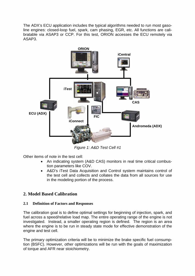
The ADX’s ECU application includes the typical algorithms needed to run most gaso-line engines: closed-loop fuel, spark, cam phasing, EGR, etc. All functions are cali-bratable via ASAP3 or CCP. For this test, ORION accesses the ECU remotely via ASAP3.

FIC iConnect

ECU (ADX)

CAS

iCentral

Andromeda (ADX)

ORION

iTest

Figure 1: A&D Test Cell #1 Other items of note in the test cell:

An indicating system (A&D CAS) monitors in real time critical combus-tion parameters like COV.

A&D’s iTest Data Acquisition and Control system maintains control of the test cell and collects and collates the data from all sources for use in the modeling portion of the process.

2. Model Based Calibration 2.1 Definition of Factors and Responses The calibration goal is to define optimal settings for beginning of injection, spark, and fuel across a speed/relative load map. The entire operating range of the engine is not investigated. Instead, a smaller operating region is defined. The region is an area where the engine is to be run in steady state mode for effective demonstration of the engine and test cell. The primary optimization criteria will be to minimize the brake specific fuel consump-tion (BSFC). However, other optimizations will be run with the goals of maximization of torque and AFR near stoichiometry.

The factors are defined as: 1. Speed 2. Relative Load 3. Beginning of Injection Timing (BOI) 4. Spark Advance Offset 5. Lambda

The responses are defined as:

1. Torque 2. Mass Fuel Flow 3. Exhaust Temperature 4. Maximum Best Torque (MBT) Spark

The optimization constraints are spark advance less than or equal to MBT Spark. No further constraints are necessary since the engine will not be operated in a manner that will produce high temperatures, high Coefficient of Variation of Indicated Mean Effective Pressure (COV of IMEP), etc. These values will be monitored during data gathering to ensure limits are not exceeded. 2.2 Experiment Design Based on the above criteria, a boundary determination experiment is performed manually on the test cell. The results of the boundary determination experiment are input into EasyDoE. Since the test cell is a development test cell, the number of points to be gathered at one time is limited to about 6 hours of operation. Therefore, the operating region is divided into two smaller speed regions for data gathering pur-poses, both with the same load range as shown in Table 1:

Table 1: Experiment Design Regions Region I Input Name Units Min

Limit Max Limit

Step Width

Speed RPM 1200 1700 100 Load % 35 67 4 BOI °ca 0 90 10 Lambda nounit 0.96 1.04 0.02 Offset Spark

Advance °ca -15 3 3

Region II Speed RPM 1700 2200 100 Load % 35 75 4 BOI °ca 0 90 10 Lambda nounit 0.96 1.04 0.02 Offset Spark

Advance °ca -15 3 3

The range of the factors is the nearly the same for each region. BOI has a value of 90° at top dead center and a value of 0° at 90° before top dead center. Spark is given as an offset value relative to MBT spark with negative values indicating a more

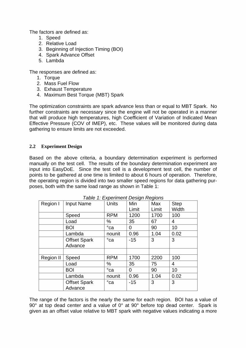
advanced spark value. This process is discussed in detail in the data gathering sec-tion. Lambda is considered 1 at an AFR of 14.57. Constraints for the experiment design are entered using 2 methods: in-equation and 2D Table. The in-equation method defines a cut-off area. The cut-off editor excludes points that meet the selected relation. In Figure 2, the upper boundary for load in Region II is defined. Points above the line between 1700 RPM / 67% load and 2200 RPM / 75% load are excluded from the candidate set.

Figure 2: High-load, Cut-off Area Determination

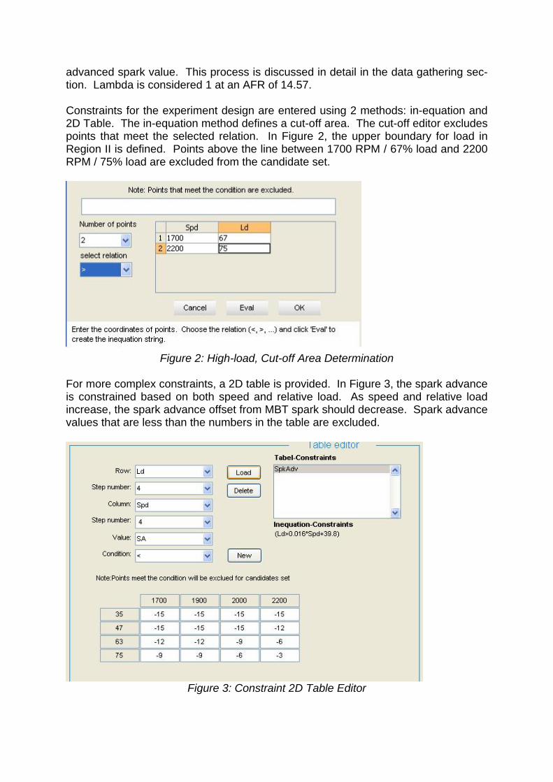
For more complex constraints, a 2D table is provided. In Figure 3, the spark advance is constrained based on both speed and relative load. As speed and relative load increase, the spark advance offset from MBT spark should decrease. Spark advance values that are less than the numbers in the table are excluded.

Figure 3: Constraint 2D Table Editor

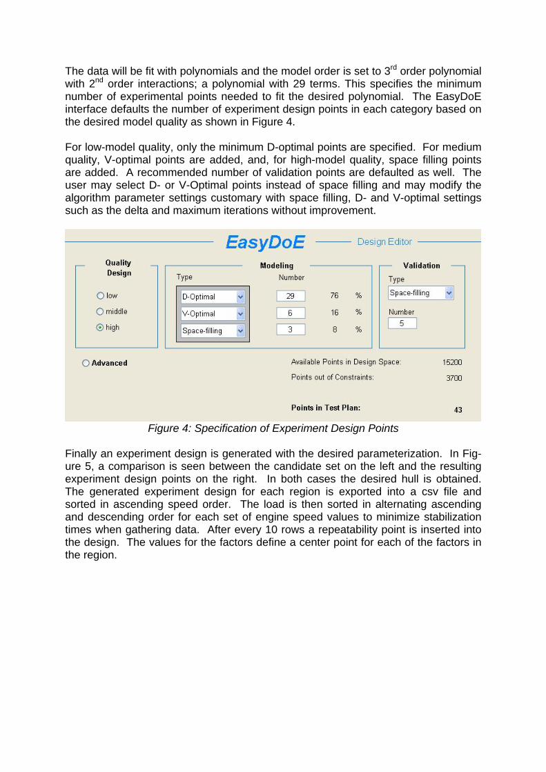
The data will be fit with polynomials and the model order is set to 3rd order polynomial with 2nd order interactions; a polynomial with 29 terms. This specifies the minimum number of experimental points needed to fit the desired polynomial. The EasyDoE interface defaults the number of experiment design points in each category based on the desired model quality as shown in Figure 4. For low-model quality, only the minimum D-optimal points are specified. For medium quality, V-optimal points are added, and, for high-model quality, space filling points are added. A recommended number of validation points are defaulted as well. The user may select D- or V-Optimal points instead of space filling and may modify the algorithm parameter settings customary with space filling, D- and V-optimal settings such as the delta and maximum iterations without improvement.

Figure 4: Specification of Experiment Design Points

Finally an experiment design is generated with the desired parameterization. In Fig-ure 5, a comparison is seen between the candidate set on the left and the resulting experiment design points on the right. In both cases the desired hull is obtained. The generated experiment design for each region is exported into a csv file and sorted in ascending speed order. The load is then sorted in alternating ascending and descending order for each set of engine speed values to minimize stabilization times when gathering data. After every 10 rows a repeatability point is inserted into the design. The values for the factors define a center point for each of the factors in the region.

Figure 5: Candidate Set and Experiment Design Points with Hull

Spark Advance vs. Speed and Load 2.3 Data Gathering Relative load is defined in equation (1) as the ratio of the mass air flow into the en-gine and the calculated 100% volumetric efficiency air mass flow at a given engine speed. Direct measurement of input mass airflow is not currently available on the test cell. Air mass flow into the engine is calculated in equation (2) using the product of the AFR signal and the fuel mass flow. Airflow at 100% volumetric efficiency is calculated using equation (3).

%100@/ airair mmRL (1)

fuelair mAFRm * (2)

2/**%100@ engairengair Vm (3)

The measurement sequence used in ORION for this test was a typical steady-state sequence. This sequence is run for all operating points defined by the DoE

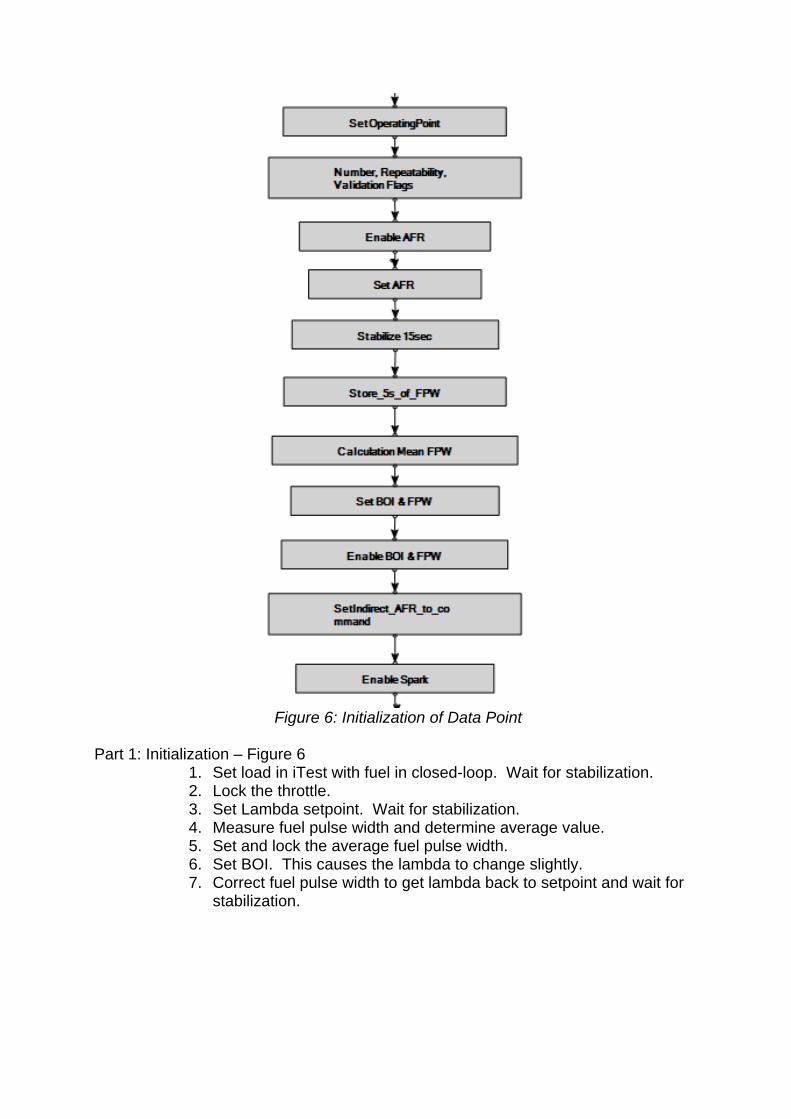
Figure 6: Initialization of Data Point

Part 1: Initialization – Figure 6

1. Set load in iTest with fuel in closed-loop. Wait for stabilization. 2. Lock the throttle. 3. Set Lambda setpoint. Wait for stabilization. 4. Measure fuel pulse width and determine average value. 5. Set and lock the average fuel pulse width. 6. Set BOI. This causes the lambda to change slightly. 7. Correct fuel pulse width to get lambda back to setpoint and wait for

stabilization.

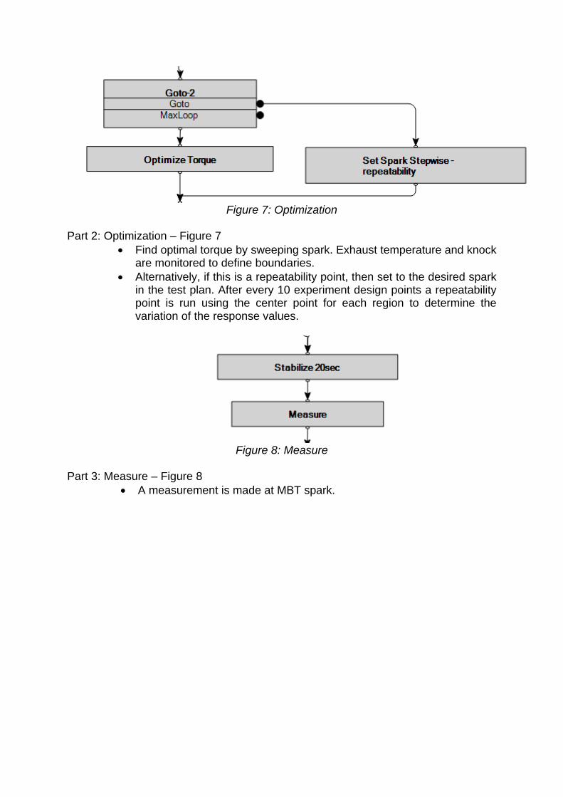
Figure 7: Optimization

Part 2: Optimization – Figure 7

Find optimal torque by sweeping spark. Exhaust temperature and knock are monitored to define boundaries.

Alternatively, if this is a repeatability point, then set to the desired spark in the test plan. After every 10 experiment design points a repeatability point is run using the center point for each region to determine the variation of the response values.

Figure 8: Measure

Part 3: Measure – Figure 8

A measurement is made at MBT spark.

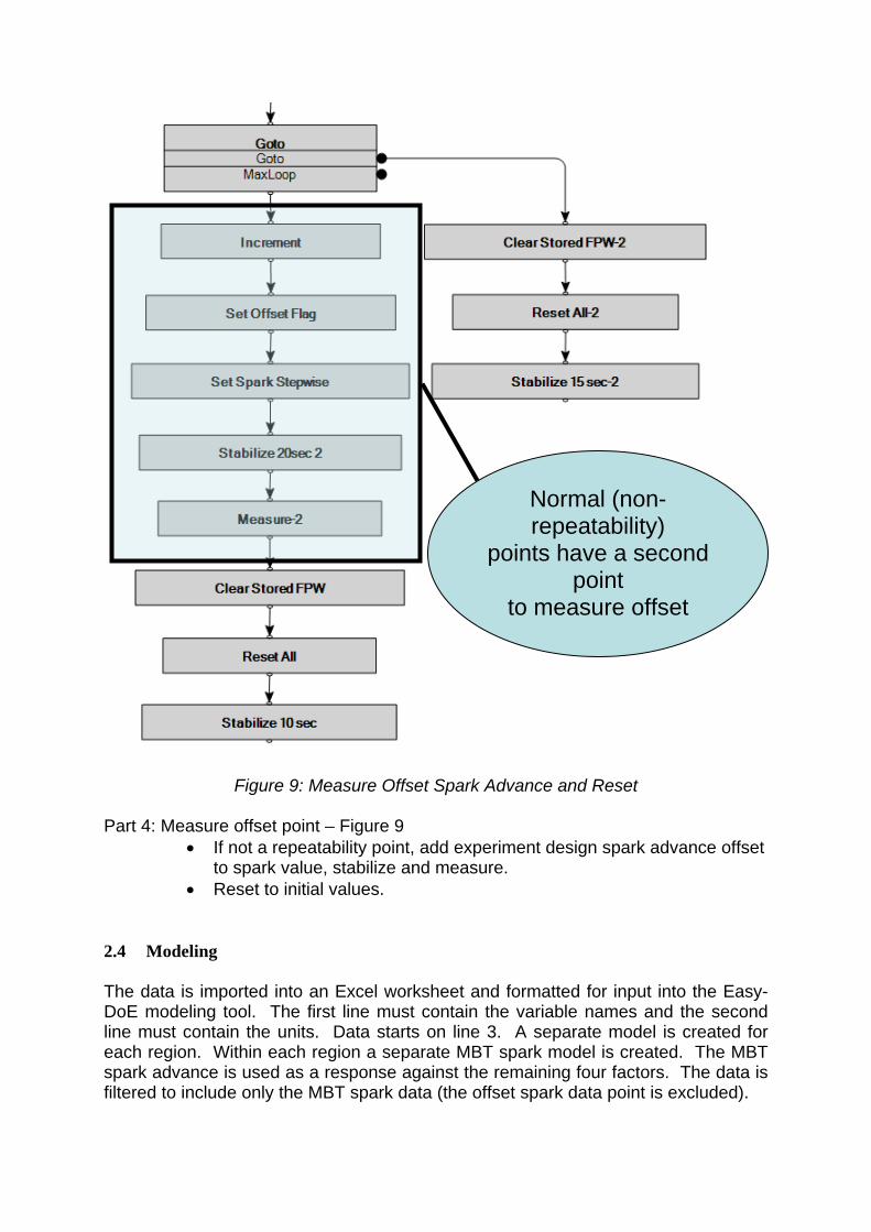
Figure 9: Measure Offset Spark Advance and Reset

Normal (non-repeatability)

points have a second point

to measure offset

Part 4: Measure offset point – Figure 9

If not a repeatability point, add experiment design spark advance offset to spark value, stabilize and measure.

Reset to initial values. 2.4 Modeling The data is imported into an Excel worksheet and formatted for input into the Easy-DoE modeling tool. The first line must contain the variable names and the second line must contain the units. Data starts on line 3. A separate model is created for each region. Within each region a separate MBT spark model is created. The MBT spark advance is used as a response against the remaining four factors. The data is filtered to include only the MBT spark data (the offset spark data point is excluded).

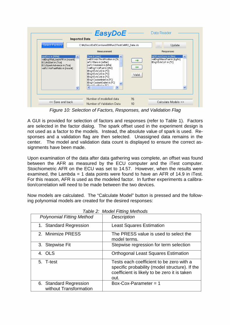
Figure 10: Selection of Factors, Responses, and Validation Flag

A GUI is provided for selection of factors and responses (refer to Table 1). Factors are selected in the factor dialog. The spark offset used in the experiment design is not used as a factor to the models. Instead, the absolute value of spark is used. Re-sponses and a validation flag are then selected. Unassigned data remains in the center. The model and validation data count is displayed to ensure the correct as-signments have been made. Upon examination of the data after data gathering was complete, an offset was found between the AFR as measured by the ECU computer and the iTest computer. Stoichiometric AFR on the ECU was set to 14.57. However, when the results were examined, the Lambda = 1 data points were found to have an AFR of 14.9 in iTest. For this reason, AFR is used as the modeled factor. In further experiments a calibra-tion/correlation will need to be made between the two devices. Now models are calculated. The “Calculate Model” button is pressed and the follow-ing polynomial models are created for the desired responses:

Table 2: Model Fitting Methods Polynomial Fitting Method Description

1. Standard Regression Least Squares Estimation

2. Minimize PRESS The PRESS value is used to select the model terms.

3. Stepwise Fit Stepwise regression for term selection

4. OLS Orthogonal Least Squares Estimation

5. T-test Tests each coefficient to be zero with a specific probability (model structure). If the coefficient is likely to be zero it is taken out.

6. Standard Regression without Transformation

Box-Cox-Parameter = 1

Polynomial Fitting Method Description

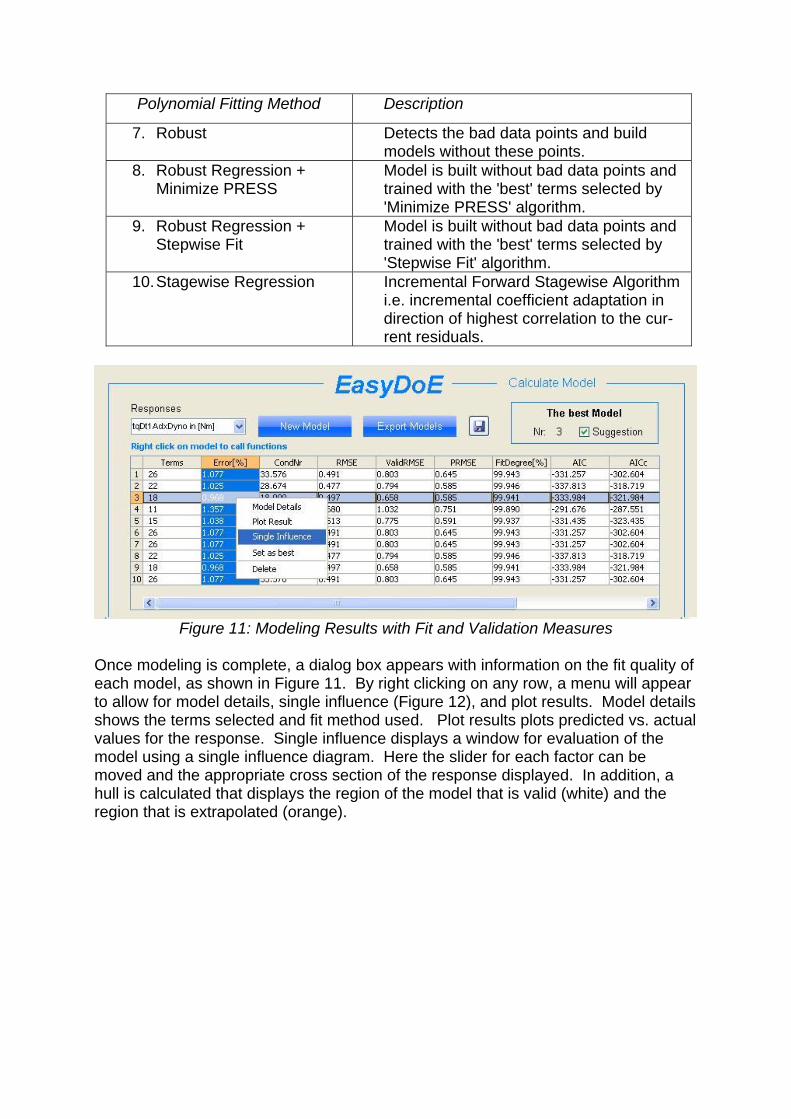
7. Robust Detects the bad data points and build models without these points.

8. Robust Regression + Minimize PRESS

Model is built without bad data points and trained with the 'best' terms selected by 'Minimize PRESS' algorithm.

9. Robust Regression + Stepwise Fit

Model is built without bad data points and trained with the 'best' terms selected by 'Stepwise Fit' algorithm.

10. Stagewise Regression Incremental Forward Stagewise Algorithm i.e. incremental coefficient adaptation in direction of highest correlation to the cur-rent residuals.

Figure 11: Modeling Results with Fit and Validation Measures

Once modeling is complete, a dialog box appears with information on the fit quality of each model, as shown in Figure 11. By right clicking on any row, a menu will appear to allow for model details, single influence (Figure 12), and plot results. Model details shows the terms selected and fit method used. Plot results plots predicted vs. actual values for the response. Single influence displays a window for evaluation of the model using a single influence diagram. Here the slider for each factor can be moved and the appropriate cross section of the response displayed. In addition, a hull is calculated that displays the region of the model that is valid (white) and the region that is extrapolated (orange).

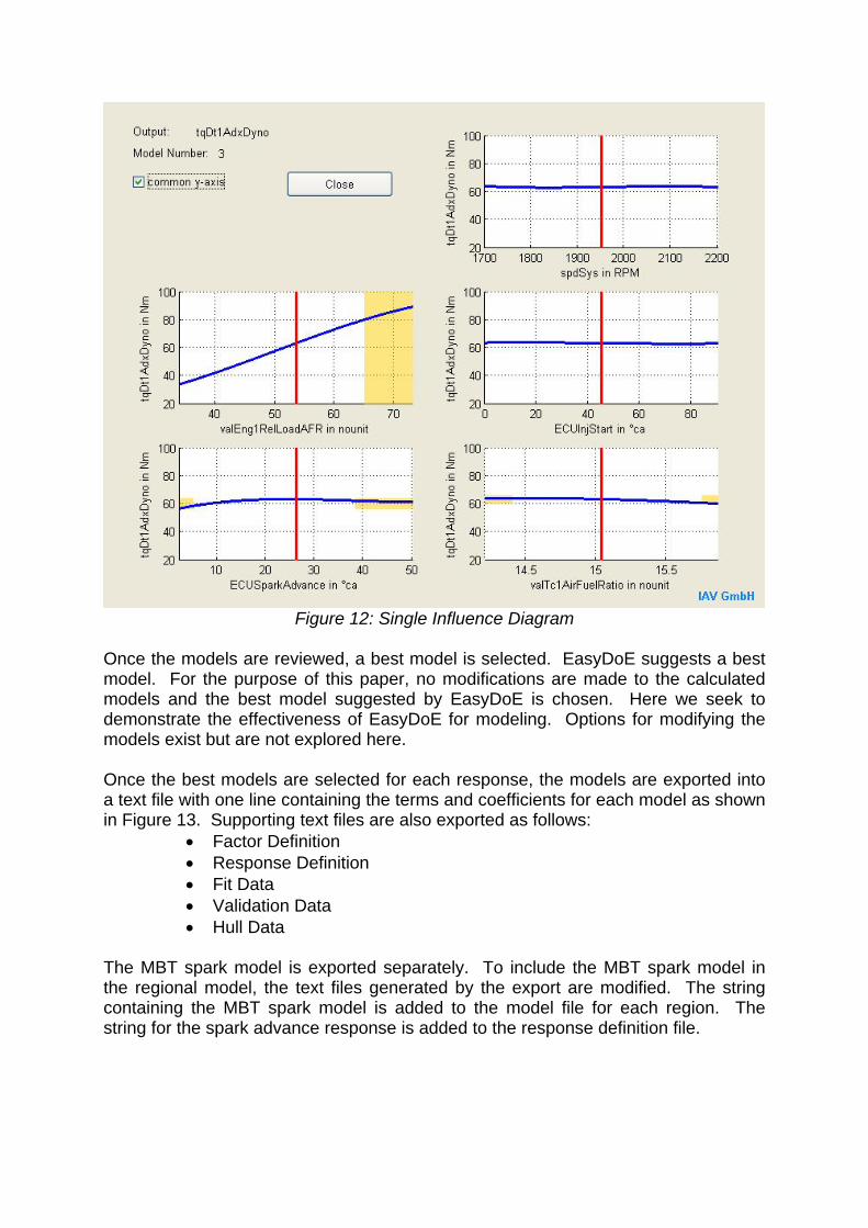
Figure 12: Single Influence Diagram

Once the models are reviewed, a best model is selected. EasyDoE suggests a best model. For the purpose of this paper, no modifications are made to the calculated models and the best model suggested by EasyDoE is chosen. Here we seek to demonstrate the effectiveness of EasyDoE for modeling. Options for modifying the models exist but are not explored here. Once the best models are selected for each response, the models are exported into a text file with one line containing the terms and coefficients for each model as shown in Figure 13. Supporting text files are also exported as follows:

Factor Definition Response Definition Fit Data Validation Data Hull Data

The MBT spark model is exported separately. To include the MBT spark model in the regional model, the text files generated by the export are modified. The string containing the MBT spark model is added to the model file for each region. The string for the spark advance response is added to the response definition file.

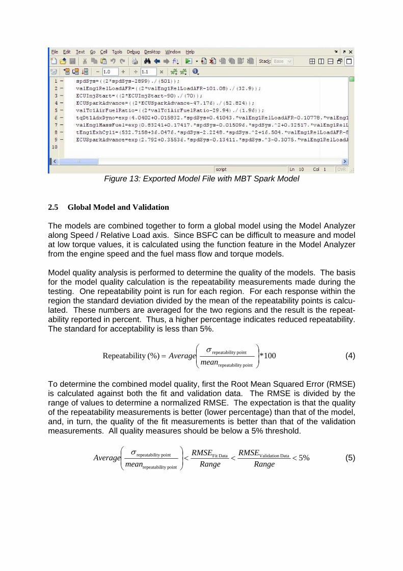
Figure 13: Exported Model File with MBT Spark Model

2.5 Global Model and Validation The models are combined together to form a global model using the Model Analyzer along Speed / Relative Load axis. Since BSFC can be difficult to measure and model at low torque values, it is calculated using the function feature in the Model Analyzer from the engine speed and the fuel mass flow and torque models. Model quality analysis is performed to determine the quality of the models. The basis for the model quality calculation is the repeatability measurements made during the testing. One repeatability point is run for each region. For each response within the region the standard deviation divided by the mean of the repeatability points is calcu-lated. These numbers are averaged for the two regions and the result is the repeat-ability reported in percent. Thus, a higher percentage indicates reduced repeatability. The standard for acceptability is less than 5%.

100*(%)ity Repeatabilpointity repeatabil

pointity repeatabil

meanAverage

(4)

To determine the combined model quality, first the Root Mean Squared Error (RMSE) is calculated against both the fit and validation data. The RMSE is divided by the range of values to determine a normalized RMSE. The expectation is that the quality of the repeatability measurements is better (lower percentage) than that of the model, and, in turn, the quality of the fit measurements is better than that of the validation measurements. All quality measures should be below a 5% threshold.

%5Data ValidationDataFit

pointity repeatabil

pointity repeatabil

Range

RMSE

Range

RMSE

meanAverage

(5)

Model Quality Analysis

0.00%

1.00%

2.00%

3.00%

4.00%

5.00%

6.00%

Torque Fuel Flow Exh Temp MBT Spark

Response

No

rmal

ized

Err

or

RepeatabilityNorm RMSE FitNorm RMSE Valid Norm RMSE Ver

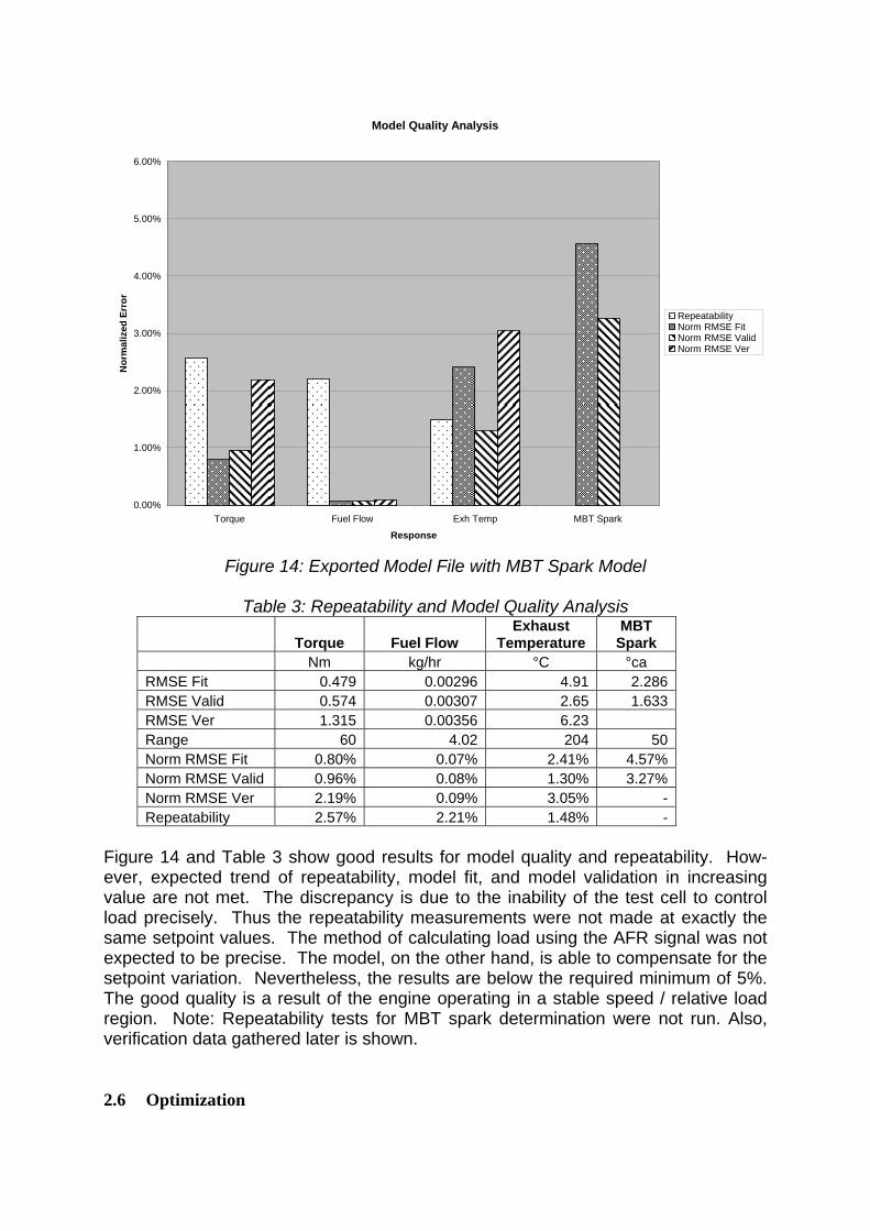
Figure 14: Exported Model File with MBT Spark Model

Table 3: Repeatability and Model Quality Analysis

Torque Fuel Flow Exhaust

Temperature MBT

Spark Nm kg/hr °C °ca

RMSE Fit 0.479 0.00296 4.91 2.286 RMSE Valid 0.574 0.00307 2.65 1.633 RMSE Ver 1.315 0.00356 6.23 Range 60 4.02 204 50 Norm RMSE Fit 0.80% 0.07% 2.41% 4.57% Norm RMSE Valid 0.96% 0.08% 1.30% 3.27% Norm RMSE Ver 2.19% 0.09% 3.05% - Repeatability 2.57% 2.21% 1.48% -

Figure 14 and Table 3 show good results for model quality and repeatability. How-ever, expected trend of repeatability, model fit, and model validation in increasing value are not met. The discrepancy is due to the inability of the test cell to control load precisely. Thus the repeatability measurements were not made at exactly the same setpoint values. The method of calculating load using the AFR signal was not expected to be precise. The model, on the other hand, is able to compensate for the setpoint variation. Nevertheless, the results are below the required minimum of 5%. The good quality is a result of the engine operating in a stable speed / relative load region. Note: Repeatability tests for MBT spark determination were not run. Also, verification data gathered later is shown. 2.6 Optimization

The optimization goal is to find settings for beginning of injection, spark advance, and air/fuel ratio (AFR) for a grid of speed / relative load points that produce a minimum BSFC. To demonstrate the effectiveness of the software tools, two other optimiza-tions are run: maximization of torque and AFR near stoichiometry. Using the Model Analyzer, a grid of speed / load points is defined:

Speed 1200 to 2200 in 100 RPM increments Relative Load 35, 45, 55, 65, 72.95 (max load)

A weighted sum gradient descent method is selected. A constraint is set to restrict the factor of spark advance to be less than the response of MBT spark. The follow-ing values are used to set the weighted sums objective function:

+1 Maximize the response - 1 Minimize the response 0 No optimization on the response

The following optimization factors are set for the three optimizations: Minimize BSFC: The optimization factor for the calculated BSFC response is set

to -1. All other optimization factors are set to 0.

Specific AFR: The optimization factor for the calculated BSFC response is set to -1. All other optimization factors are set to 0. An additional constraint is added so that AFR < 15.00.

Maximum torque: The optimization factor for torque is set to 1, and all others are set to 0.

2.7 Factor Maps and Verification To validate the models and the optimization method, verification tests are run on the test cell. A grid of speed / relative load points is run with the values of BOI, Spark Advance, and AFR determined by the optimization.

Speed: 1200 to 2100 in 300 RPM increments Relative Load: 35, 45, 55, 65

Three sets of BOI/Spark/AFR values are run against the same speed / relative load setpoints. A MATLAB script performs the following comparisons:

Model vs. Measured – To validate model quality at the optimal solutions

Optimization Setpoints – To compare inputs based on optimization criteria

Optimization Responses – To show the optimization produces the desired effect

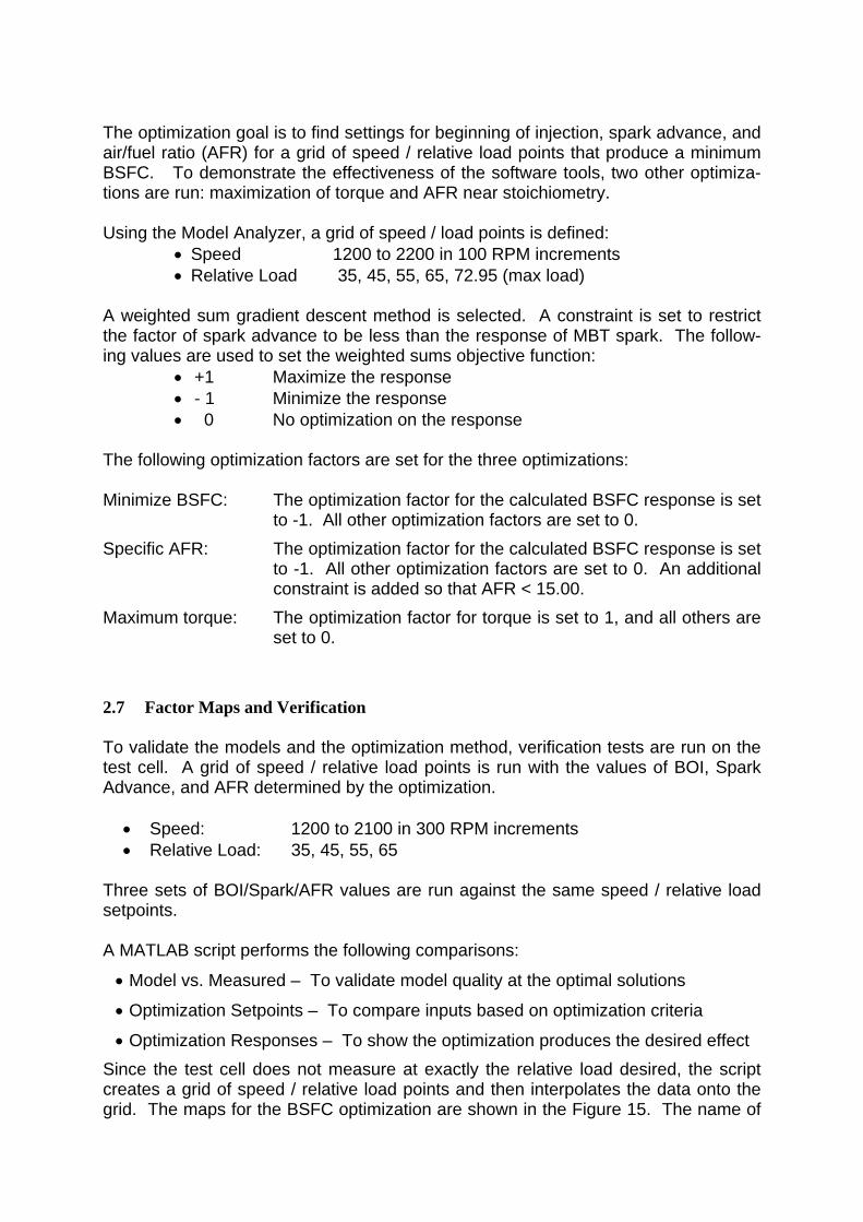
Since the test cell does not measure at exactly the relative load desired, the script creates a grid of speed / relative load points and then interpolates the data onto the grid. The maps for the BSFC optimization are shown in the Figure 15. The name of

the variable plotted on the z-axis is given in the title of the graph. The text in paren-thesis is the data set being used:

BSFC: Verification Data – BSFC Optimization Torque: Verification Data – Torque optimization BSFCModel: Model outputs using the inputs from the BSFC verification data*

TorqueModel: Model outputs using the inputs from the Torque verification data*

* For the BSFCModel and TorqueModel data sets, the values of the factors

measured at the test cell are input back into the model and the corresponding output values predicted.

The factor maps for the BSFC optimization are shown in Figure 15. As expected, the AFR is a smooth surface that is relatively lean. The corresponding spark advance map is relatively smooth as well with spark advance decreasing for increasing load. The BOI map shows a valley in the center. BOI has a greater effect on emissions than fuel consumption, so the optimizer seems to have more freedom to choose a value. Further testing will include emissions analysis and BOI will have a greater weight in the optimization.

12001400

16001800

20002200

40

60

0

20

40

60

80

EngSpd in RPM

BOI(BSFCModel) in deg

RelLd in %

403020

2010

30

BOI(BSFCModel) in deg

EngSpd in RPM

40

5040

Rel

Ld in

%

1200 1400 1600 1800 2000 220030

40

50

60

70

12001400

16001800

20002200

40

60

0

10

20

30

40

50

EngSpd in RPM

SA(BSFCModel) in deg

RelLd in %

2322

20

21

20

23

1918

SA(BSFCModel) in deg

EngSpd in RPM

22

18

21

17

Rel

Ld in

%

1200 1400 1600 1800 2000 220030

40

50

60

70

12001400

16001800

20002200

40

60

14

14.5

15

15.5

16

EngSpd in RPM

AFR(BSFCModel) in nounit

RelLd in %

15.6

15.5

15.4

15.6

AFR(BSFCModel) in nounit

EngSpd in RPM

15.715

.815.9

Rel

Ld in

%

1200 1400 1600 1800 2000 220030

40

50

60

70

Figure 15: BSFC Optimization: BOI, Spark, AFR Setpoints

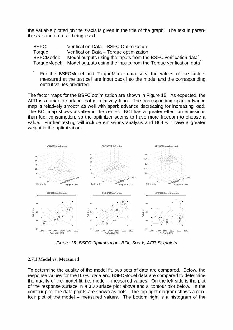
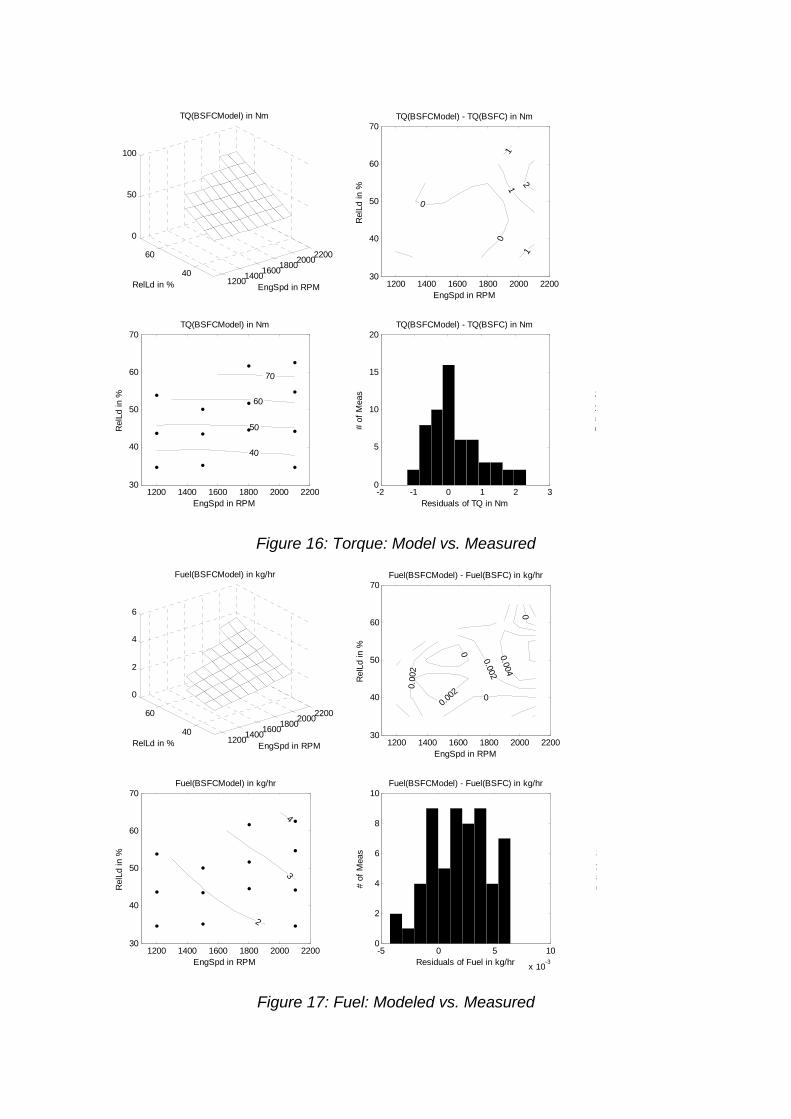
2.7.1 Model vs. Measured To determine the quality of the model fit, two sets of data are compared. Below, the response values for the BSFC data and BSFCModel data are compared to determine the quality of the model fit, i.e. model – measured values. On the left side is the plot of the response surface in a 3D surface plot above and a contour plot below. In the contour plot, the data points are shown as dots. The top-right diagram shows a con-tour plot of the model – measured values. The bottom right is a histogram of the

model – measured values at the interpolated grid points. The expectation is that the histogram will be Gaussian in shape with a mean about zero. In Figure 16, the torque response behaves as expected with torque increasing with relative load and slightly decreasing with speed. The error is less than 2 Nm and tends to increase with speed, indicating the model structure does not capture torque completely. In Figure 17, the fuel model predicts very well, with mass fuel flow increasing with both speed and relative load. The error is very small, on the order of 2-3 grams/hr and evenly distributed over the surface. This is expected as fuel flow is linear. How-ever, the error is usually positive and not distributed about zero. In Figure 18, exhaust temperature also predicts very well, with exhaust temperature increasing with increasing speed and relative load. The error is small and between +/- 5 ºC. In Figure 19, the calculated BSFC response shows decreasing specific fuel con-sumption with increasing load. The engine is not run hard enough to show a mini-mum. The error is very small and symmetric about zero.

12001400

16001800

20002200

40

60

0

50

100

EngSpd in RPM

TQ(BSFCModel) in Nm

RelLd in %

70

60

40

50

TQ(BSFCModel) in Nm

EngSpd in RPM

Rel

Ld in

%

1200 1400 1600 1800 2000 220030

40

50

60

70

RlL

di

%

0

01

1

1

2

EngSpd in RPM

Rel

Ld in

%

TQ(BSFCModel) - TQ(BSFC) in Nm

1200 1400 1600 1800 2000 220030

40

50

60

70

-2 -1 0 1 2 30

5

10

15

20

Residuals of TQ in Nm

# of

Mea

s

TQ(BSFCModel) - TQ(BSFC) in Nm

Figure 16: Torque: Model vs. Measured

12001400

16001800

20002200

40

60

0

2

4

6

EngSpd in RPM

Fuel(BSFCModel) in kg/hr

RelLd in %

4

3

2

Fuel(BSFCModel) in kg/hr

EngSpd in RPM

Rel

Ld in

%

1200 1400 1600 1800 2000 220030

40

50

60

70

RlL

di

%

0

0

0

0.00

2

0.002

0.00

2

0.004

EngSpd in RPM

Rel

Ld in

%

Fuel(BSFCModel) - Fuel(BSFC) in kg/hr

1200 1400 1600 1800 2000 220030

40

50

60

70

-5 0 5 10

x 10-3

0

2

4

6

8

10

Residuals of Fuel in kg/hr

# of

Mea

s

Fuel(BSFCModel) - Fuel(BSFC) in kg/hr

Figure 17: Fuel: Modeled vs. Measured

12001400

16001800

20002200

40

60

0

500

1000

EngSpd in RPM

Exh Temp(BSFCModel) in DegC

RelLd in %

580

560

Exh Temp(BSFCModel) in DegC

EngSpd in RPM

540

520

500

480

Rel

Ld in

%

1200 1400 1600 1800 2000 220030

40

50

60

70

RlL

di

%

-7 -5 -3 -1

-1

1

1

1

3

3

3

5

5EngSpd in RPM

Rel

Ld in

%

Exh Temp(BSFCModel) - Exh Temp(BSFC) in degC

1200 1400 1600 1800 2000 220030

40

50

60

70

-15 -10 -5 0 5 100

5

10

15

20

Residuals of Exh Temp in DegC

# of

Mea

s

Exh Temp(BSFCModel) - Exh Temp(BSFC) in degC

Figure 18: Exhaust Temperature: Modeled vs. Measured

12001400

16001800

20002200

40

60

200

250

300

350

400

EngSpd in RPM

Spec Fuel(BSFCModel) in g/kW.hr

RelLd in %

240

260

250

270

280

Spec Fuel(BSFCModel) in g/kW.hr

EngSpd in RPM

290

Rel

Ld in

%

1200 1400 1600 1800 2000 220030

40

50

60

70

RlL

di

%

-7-7

-4

-4-1

2

2

58

EngSpd in RPM

Rel

Ld in

%

Spec Fuel(BSFCModel) - Spec Fuel(BSFC) in g/kW.hr

1200 1400 1600 1800 2000 220030

40

50

60

70

-15 -10 -5 0 5 10 150

5

10

15

20

Residuals of Spec Fuel in g/kW.hr

# of

Mea

s

Spec Fuel(BSFCModel) - Spec Fuel(BSFC) in g/kW.hr

Figure 19: BSFC Modeled (calculated) vs. Measured

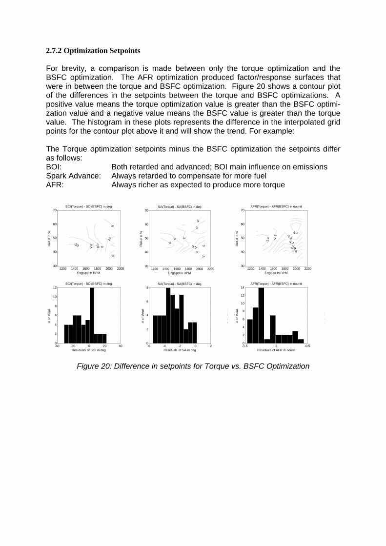
2.7.2 Optimization Setpoints For brevity, a comparison is made between only the torque optimization and the BSFC optimization. The AFR optimization produced factor/response surfaces that were in between the torque and BSFC optimization. Figure 20 shows a contour plot of the differences in the setpoints between the torque and BSFC optimizations. A positive value means the torque optimization value is greater than the BSFC optimi-zation value and a negative value means the BSFC value is greater than the torque value. The histogram in these plots represents the difference in the interpolated grid points for the contour plot above it and will show the trend. For example: The Torque optimization setpoints minus the BSFC optimization the setpoints differ as follows: BOI: Both retarded and advanced; BOI main influence on emissions Spark Advance: Always retarded to compensate for more fuel AFR: Always richer as expected to produce more torque

-30

-20

-10 0

0

010

EngSpd in RPM

Rel

Ld in

%

BOI(Torque) - BOI(BSFC) in deg

1200 1400 1600 1800 2000 220030

40

50

60

70

-40 -20 0 20 400

2

4

6

8

10

12

Residuals of BOI in deg

# of

Mea

s

BOI(Torque) - BOI(BSFC) in deg

RlL

di

%

-5

-4

-3

-3

-2-2

-1

-1

0

0

EngSpd in RPM

Rel

Ld in

%

SA(Torque) - SA(BSFC) in deg

1200 1400 1600 1800 2000 220030

40

50

60

70

-6 -4 -2 0 20

2

4

6

8

Residuals of SA in deg

# of

Mea

s

SA(Torque) - SA(BSFC) in deg

RlL

di

%

-1.4 -1

.3

-1.3-1.2

-1.1-1

-0.9-0.8

EngSpd in RPM

Rel

Ld in

%

AFR(Torque) - AFR(BSFC) in nounit

1200 1400 1600 1800 2000 220030

40

50

60

70

-1.5 -1 -0.50

2

4

6

8

10

12

14

Residuals of AFR in nounit

# of

Mea

s

AFR(Torque) - AFR(BSFC) in nounit

Figure 20: Difference in setpoints for Torque vs. BSFC Optimization

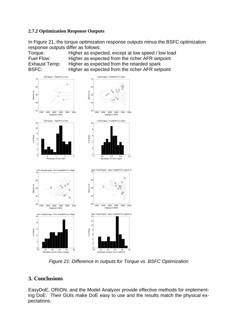
2.7.2 Optimization Response Outputs In Figure 21, the torque optimization response outputs minus the BSFC optimization response outputs differ as follows: Torque: Higher as expected, except at low speed / low load Fuel Flow: Higher as expected from the richer AFR setpoint Exhaust Temp: Higher as expected from the retarded spark BSFC: Higher as expected from the richer AFR setpoint

RlL

di

%

0

1

2

2

EngSpd in RPM

Rel

Ld in

%

TQ(Torque) - TQ(BSFC) in Nm

1200 1400 1600 1800 2000 220030

40

50

60

70

-1 0 1 2 30

2

4

6

8

10

12

Residuals of TQ in Nm

# of

Mea

s

TQ(Torque) - TQ(BSFC) in Nm

RlL

di

%

0.15

0.18

0.21

0.24

0.27

0.3

0.3 0.33

EngSpd in RPM

Rel

Ld in

%

Fuel(Torque) - Fuel(BSFC) in kg/hr

1200 1400 1600 1800 2000 220030

40

50

60

70

0 0.1 0.2 0.3 0.40

2

4

6

8

10

Residuals of Fuel in kg/hr

# of

Mea

s

Fuel(Torque) - Fuel(BSFC) in kg/hr

RlL

di

%

15

15

17

19

21

23

25

27

29

EngSpd in RPM

Rel

Ld in

%

Exh Temp(Torque) - Exh Temp(BSFC) in degC

1200 1400 1600 1800 2000 220030

40

50

60

70

10 15 20 25 30 350

2

4

6

8

10

Residuals of Exh Temp in DegC

# of

Mea

s

Exh Temp(Torque) - Exh Temp(BSFC) in degC

RlL

di

%

12

13

13

13

1415

16

17

17

18

19

EngSpd in RPM

Rel

Ld in

%

Spec Fuel(Torque) - Spec Fuel(BSFC) in g/kW.hr

1200 1400 1600 1800 2000 220030

40

50

60

70

10 12 14 16 18 200

2

4

6

8

10

12

14

Residuals of Spec Fuel in g/kW.hr

# of

Mea

s

Spec Fuel(Torque) - Spec Fuel(BSFC) in g/kW.hr

Figure 21: Difference in outputs for Torque vs. BSFC Optimization

3. Conclusions EasyDoE, ORION, and the Model Analyzer provide effective methods for implement-ing DoE. Their GUIs make DoE easy to use and the results match the physical ex-pectations.

The Authors: Anthony J. Gullitti BS, MS Chemical Engineering, IAV Inc., Northville, MI USA Donald Nutter BS, MS, Computer Science, A&D Technology, Ann Arbor, MI USA