Demonstration of Passive Acoustic Detection and Tracking of ...

Demonstration of Passive Acoustic Detection andTracking of Unmanned Underwater Vehicles

byKristen Elizabeth Railey

S.B. Mechanical Engineering, Massachusetts Institute of Technology (2013)Submitted to the Department of Mechanical Engineeringin partial fulfillment of the requirements for the degree of

Master of Science in Mechanical Engineeringat the

MASSACHUSETTS INSTITUTE OF TECHNOLOGYand the

WOODS HOLE OCEANOGRAPHIC INSTITUTIONJune 2018

c○ 2018 Kristen Elizabeth Railey. All rights reserved.The author hereby grants to MIT, WHOI, and The Charles Stark Draper Laboratory, Inc.permission to reproduce and to distribute publicly paper and electronic copies of this thesis

document in whole or in part in any medium now known or hereafter created.

Author . . . . . . . . . . . . . . . . . . . . . . . . . . . . . . . . . . . . . . . . . . . . . . . . . . . . . . . . . . . . . . . . . . . . . . . . . . . . . . . . . . .Department of Mechanical Engineering

May 23, 2018

Certified by . . . . . . . . . . . . . . . . . . . . . . . . . . . . . . . . . . . . . . . . . . . . . . . . . . . . . . . . . . . . . . . . . . . . . . . . . . . . . .Henrik Schmidt

Professor of Mechanical and Ocean EngineeringMassachusetts Institute of Technology

Thesis Supervisor

Certified by . . . . . . . . . . . . . . . . . . . . . . . . . . . . . . . . . . . . . . . . . . . . . . . . . . . . . . . . . . . . . . . . . . . . . . . . . . . . . .Dino Dibiaso

Senior Project LeaderThe Charles Stark Draper Laboratory, Inc.

Thesis SupervisorAccepted by . . . . . . . . . . . . . . . . . . . . . . . . . . . . . . . . . . . . . . . . . . . . . . . . . . . . . . . . . . . . . . . . . . . . . . . . . . . . . .

Rohan AbeyaratneChairman, Department Committee on Graduate Theses

Massachusetts Institute of Technology

Accepted by . . . . . . . . . . . . . . . . . . . . . . . . . . . . . . . . . . . . . . . . . . . . . . . . . . . . . . . . . . . . . . . . . . . . . . . . . . . . . .Henrik Schmidt

Chairman, Joint Committee for Applied Ocean Science & EngineeringMassachusetts Institute of TechnologyWoods Hole Oceanographic Institution

2

Demonstration of Passive Acoustic Detection and Tracking of

Unmanned Underwater Vehicles

by

Kristen Elizabeth Railey

Submitted to the Department of Mechanical Engineeringon May 23, 2018, in partial fulfillment of the

requirements for the degree ofMaster of Science in Mechanical Engineering

AbstractIn terms of national security, the advancement of unmanned underwater vehicle(UUV) technology has transformed UUVs from tools for intelligence, surveillance,and reconnaissance and mine countermeasures to autonomous platforms that canperform complex tasks like tracking submarines, jamming, and smart mining. To-day, they play a major role in asymmetric warfare, as UUVs have attributes that aredesirable for less-established navies. They are covert, easy to deploy, low-cost, andlow-risk to personnel. The concern of protecting against UUVs of malicious intent isthat existing defense systems fall short in detecting, tracking, and preventing the ve-hicles from causing harm. Addressing this gap in technology, this thesis is the first todemonstrate passively detecting and tracking UUVs in realistic environments strictlyfrom the vehicle’s self-generated noise. This work contributes the first power spectraldensity estimate of an underway micro-UUV, field experiments in a pond and riverdetecting a UUV with energy thresholding and spectral filters, and field experimentsin a pond and river tracking a UUV using conventional and adaptive beamforming.The spectral filters resulted in a probability of detection of 96% and false alarmsof 18% at a distance of 100m, with boat traffic in a river environment. Trackingthe vehicle with adaptive beamforming resulted in a 6.2± 5.7 ∘ absolute difference inbearing. The principal achievement of this work is to quantify how well a UUV canbe covertly tracked with knowledge of its spectral features. This work can be imple-mented into existing passive acoustic surveillance systems and be applied to largerclasses of UUVs, which potentially have louder identifying acoustic signatures.

Thesis Supervisor: Henrik SchmidtTitle: Professor of Mechanical and Ocean EngineeringMassachusetts Institute of Technology

Thesis Supervisor: Dino DibiasoTitle: Senior Project LeaderThe Charles Stark Draper Laboratory, Inc.

3

4

Acknowledgments

Most of all, I would like to thank Henrik Schmidt for his support of me as a researcher and

student. Thank you for all your advice on my thesis and coursework. Also thank you for

advocating for me and believing in me as a researcher.

I would also like to thank my co-supervisor, Dino DiBiaso, for his support and guidance

– not only on my thesis research but also for my experience at Draper Labs. Thank you for

all your feedback and encouragement.

Next I would like to thank all of my colleagues in the Laboratory of Autonomous Marine

Sensing Systems – especially Mike Benjamin, Misha Novitzky, Caileigh Fitzgerald, Paul

Robinette, Eeshan Bhatt, Rui Chen, Oscar Viquez, Nick Rypkema, Greg Nannig, and Erin

Fischell. Thank you for your support, guidance, and friendship.

I’d also like to recognize Joe Edwards, Nick Pulsone, and Doug Hart for their mentorship

while at MIT as an undergrad and at MIT Lincoln Laboratory. You inspired me to pursue

my master’s degree in mechanical engineering, specializing in ocean robotics.

Finally I want to thank my friends and family, especially my parents – Cheryl and

Malcolm – and my brothers – Owen and Stuart – for always being there for me. I could not

have accomplished this without you. And thank you to Derek, for being my best friend and

support system.

To make this research possible, I am grateful for the support from the National De-

fense Science and Engineering Graduate Fellowship and Draper Labs Fellowship, as well as

DARPA for the support of the Bluefin Sandshark unmanned underwater vehicle.

This research was conducted with Government support under and awarded by DoD,

Air Force Office of Scientific Research, National Defense Science and Engineering Graduate

(NDSEG) Fellowship, 32 CFR 168a.

5

6

Contents

1 Introduction 19

2 Background 23

2.1 Current State of Technology and Vulnerabilities in UUVs . . . . . . . . . . . . 23

2.1.1 Hull and Propulsion Design . . . . . . . . . . . . . . . . . . . . . . . . 24

2.1.2 Stability . . . . . . . . . . . . . . . . . . . . . . . . . . . . . . . . . . . 25

2.1.3 Energy . . . . . . . . . . . . . . . . . . . . . . . . . . . . . . . . . . . . 26

2.1.4 Autonomy . . . . . . . . . . . . . . . . . . . . . . . . . . . . . . . . . . 27

2.1.5 Communication . . . . . . . . . . . . . . . . . . . . . . . . . . . . . . . 28

2.1.6 Sensors . . . . . . . . . . . . . . . . . . . . . . . . . . . . . . . . . . . 29

2.1.7 Navigation . . . . . . . . . . . . . . . . . . . . . . . . . . . . . . . . . 30

2.2 Applications of UUVs . . . . . . . . . . . . . . . . . . . . . . . . . . . . . . . 31

2.2.1 Current Missions . . . . . . . . . . . . . . . . . . . . . . . . . . . . . . 32

2.2.2 Future Missions . . . . . . . . . . . . . . . . . . . . . . . . . . . . . . . 32

2.3 Motivation for Detecting and Tracking UUVs . . . . . . . . . . . . . . . . . . 33

2.3.1 U.S. Navy . . . . . . . . . . . . . . . . . . . . . . . . . . . . . . . . . . 34

2.3.2 DARPA . . . . . . . . . . . . . . . . . . . . . . . . . . . . . . . . . . . 34

2.3.3 Rapid Reaction Technology Office . . . . . . . . . . . . . . . . . . . . 35

2.3.4 Defense Science Board . . . . . . . . . . . . . . . . . . . . . . . . . . . 35

3 Related Work 37

3.1 Acoustic Spectrum Analysis of UUVs . . . . . . . . . . . . . . . . . . . . . . . 37

3.2 Automatic Target Recognition . . . . . . . . . . . . . . . . . . . . . . . . . . . 38

3.2.1 Detection with Active Sonar . . . . . . . . . . . . . . . . . . . . . . . . 39

3.2.2 Detection with Passive Sonar . . . . . . . . . . . . . . . . . . . . . . . 39

7

3.3 Passive Acoustic Tracking . . . . . . . . . . . . . . . . . . . . . . . . . . . . . 40

4 Detection and Tracking Theory 43

4.1 Detection Threshold Theory . . . . . . . . . . . . . . . . . . . . . . . . . . . 43

4.1.1 Passive Sonar Equation . . . . . . . . . . . . . . . . . . . . . . . . . . 43

4.1.2 Receiver Operating Characteristic Curves . . . . . . . . . . . . . . . . 44

4.2 Power Spectral Density . . . . . . . . . . . . . . . . . . . . . . . . . . . . . . . 45

4.3 Underway Vehicle Detection . . . . . . . . . . . . . . . . . . . . . . . . . . . . 46

4.3.1 Short-Time Fourier Transform . . . . . . . . . . . . . . . . . . . . . . . 46

4.3.2 Energy Calculation . . . . . . . . . . . . . . . . . . . . . . . . . . . . . 46

4.3.3 Spectral Filters . . . . . . . . . . . . . . . . . . . . . . . . . . . . . . . 47

4.3.4 Summary . . . . . . . . . . . . . . . . . . . . . . . . . . . . . . . . . . 48

4.4 Beamforming . . . . . . . . . . . . . . . . . . . . . . . . . . . . . . . . . . . . 49

4.4.1 Uniform Linear Arrays . . . . . . . . . . . . . . . . . . . . . . . . . . . 49

4.4.2 Weighted Linear Arrays . . . . . . . . . . . . . . . . . . . . . . . . . . 54

4.4.3 Array Steering . . . . . . . . . . . . . . . . . . . . . . . . . . . . . . . 55

4.4.4 Beamforming on a Moving Target . . . . . . . . . . . . . . . . . . . . . 57

4.4.5 Minimum Power Distortionless Response (MPDR) Beamformer . . . . 58

5 Experimental Methods 61

5.1 Bluefin Sandshark UUV . . . . . . . . . . . . . . . . . . . . . . . . . . . . . . 61

5.1.1 Tetrahedral Array . . . . . . . . . . . . . . . . . . . . . . . . . . . . . 62

5.1.2 Autonomy – MOOS-IvP . . . . . . . . . . . . . . . . . . . . . . . . . . 63

5.2 Horizontal Line Array . . . . . . . . . . . . . . . . . . . . . . . . . . . . . . . 64

5.3 Power Spectral Density Estimate – Test Setup . . . . . . . . . . . . . . . . . . 64

5.4 Jenkins Pond Demonstration – Test Setup . . . . . . . . . . . . . . . . . . . . 65

5.5 Charles River Demonstration – Test Setup . . . . . . . . . . . . . . . . . . . . 67

6 Field Experiments and Results 73

6.1 Power Spectral Density Estimate – Results . . . . . . . . . . . . . . . . . . . . 73

6.2 Jenkins Pond Demonstration – Results . . . . . . . . . . . . . . . . . . . . . . 75

6.2.1 Detection . . . . . . . . . . . . . . . . . . . . . . . . . . . . . . . . . . 75

6.2.2 Tracking . . . . . . . . . . . . . . . . . . . . . . . . . . . . . . . . . . . 76

8

6.3 Charles River Demonstration – Results . . . . . . . . . . . . . . . . . . . . . . 80

6.3.1 Detection . . . . . . . . . . . . . . . . . . . . . . . . . . . . . . . . . . 81

6.3.2 Tracking . . . . . . . . . . . . . . . . . . . . . . . . . . . . . . . . . . . 84

7 Conclusion 89

9

10

List of Figures

2-1 Bluefin Robotics line of UUVs: Bluefin Robotics, a major manufacturer of

UUVs, produces a range of UUVs that vary by depth rating, which relates to

the size of the vehicle. The Hovering AUV (HAUV) is the only vehicle they

manufacturer that does not have a torpedo-shaped hull and single propeller

design [1]. . . . . . . . . . . . . . . . . . . . . . . . . . . . . . . . . . . . . . . 25

4-1 Windowing effect on incoming signal 𝑥(𝑡): when a window function, 𝑤(𝑡), is

applied to the signal, the signal becomes segmented, which is used for short-

time Fourier transform [55]. . . . . . . . . . . . . . . . . . . . . . . . . . . . . 47

4-2 Frequency response of ideal low pass filter: frequencies that are passed through

are between positive and negative 𝑤, frequencies that are eliminated are rep-

resented by the stop-band [78]. . . . . . . . . . . . . . . . . . . . . . . . . . . 47

4-3 Process for producing ROC curves on a moving target: incoming data from

a hydrophone element is analyzed by applying short-time Fourier transform,

spectral filtering, and energy thresholding. The result is compared to the

true presence of the UUV to calculate probabilities of false alarms and true

detections. . . . . . . . . . . . . . . . . . . . . . . . . . . . . . . . . . . . . . . 49

4-4 Coordinate system for beamforming: elevation and azimuth are defined as 𝜃

and 𝜑 respectively. . . . . . . . . . . . . . . . . . . . . . . . . . . . . . . . . . 50

4-5 Coordinates and element spacing of a line array: a vertical line array measures

direction of arrival in elevation, or 𝜃. The elements, which are identified by

numbers 0 to 𝑁 are evenly spaced by Δ𝑧 [94]. . . . . . . . . . . . . . . . . . . 50

4-6 Filtering process of an array in visual form: the incoming signal on each

element of the array 𝑓(𝑡, 𝑝𝑛) is filtered by ℎ𝑛(𝜏) and summed together to

produce the array output 𝑦(𝑡) [94]. . . . . . . . . . . . . . . . . . . . . . . . . 51

11

4-7 Delay and sum beamforming process in visual form: the signal on each ele-

ment of the array, 𝑓(𝑡−𝜏𝑛), is filtered by applying a delay, ℎ𝑛(𝜏), and summed

together to produce the array output 𝑦(𝑡) [94]. . . . . . . . . . . . . . . . . . 53

4-8 Weights for a narrowband beamformer: gain and phase can be modified to

create an optimal beamformer [94]. . . . . . . . . . . . . . . . . . . . . . . . . 53

4-9 Comparison of Kaiser and uniform weights: the tradeoff between Kaiser and

uniform weights is side lobe height and beamwidth. Kaiser weighting de-

creases side lobe heights but widens the beamwidth [94]. . . . . . . . . . . . . 55

4-10 Theoretical beampatterns of Charles River array configuration: in each sub-

plot, uniform (blue) and Kaiser (red) weightings are compared. The top

figures are beampatterns at 10,000 Hz, the cutoff frequency for spatial alias-

ing in this configuration. The bottom figures are beampatterns at 5,000 Hz,

half of the cutoff frequency for spatial aliasing. The left plots are steered to

broadside or 90𝑜, the right plots are steered to 135𝑜. . . . . . . . . . . . . . . 56

4-11 Theoretical beampatterns of Jenkins Pond array configuration: in each sub-

plot, uniform (blue) and Kaiser (red) weightings are compared. The top

figures are beampatterns at 3,000 Hz, the cutoff frequency for spatial alias-

ing in this configuration. The bottom figures are beampatterns at 1,500 Hz,

half of the cutoff frequency for spatial aliasing. The left plots are steered to

broadside or 90𝑜, the right plots are steered to 135𝑜. . . . . . . . . . . . . . . 57

4-12 Beamforming process for a moving target: to estimate bearing of a moving

target, the incoming signal on each array element is segmented into time snap-

shots, discrete Fourier transform is applied, and frequencies are individually

beamformed. The beamformer results across all frequencies are averaged,

resulting in a beamformer output over time. . . . . . . . . . . . . . . . . . . . 58

5-1 Bluefin Sandshark micro-UUV: this micro-UUV manufactured by Bluefin

Robotics was used to demonstrate passive detection and tracking in a pond

and river experiment [73]. . . . . . . . . . . . . . . . . . . . . . . . . . . . . . 61

5-2 Tetrahedral array in nose payload section of the Bluefin Sandshark micro-UUV. 63

12

5-3 Element configuration of a tetrahedral array: a tetrahedral array is in the

nose payload section of the micro-UUV, which was used to collect acoustic

data for the PSD estimate of the vehicle. . . . . . . . . . . . . . . . . . . . . . 63

5-4 Hydrophone element HTI-96-MIN: this hydrophone was used to measure the

power spectral density estimate of the micro-UUV. Four of the hydrophones

are configured in a tetrahedral array in the nose of the Bluefin Sandshark

micro-UUV used in these experiments [6]. . . . . . . . . . . . . . . . . . . . . 64

5-5 Autonomy decision-making process of MOOS-IvP software: MOOS-IvP is

configured such that the vehicle computer is separate from the autonomy

payload [5]. . . . . . . . . . . . . . . . . . . . . . . . . . . . . . . . . . . . . . 64

5-6 Diagram of the horizontal line array and data acquisition setup: data from

the horizontal line array was collected using an analog to digital converter,

data storage unit, GPS trigger, and power. . . . . . . . . . . . . . . . . . . . . 65

5-7 Power spectral density estimate experiment at the MIT alumni pool: the

Bluefin Sandshark micro-UUV was secured while its propellor revolved at

approximately 1.5m/s. The onboard acoustic sensors collected acoustic noise

data. . . . . . . . . . . . . . . . . . . . . . . . . . . . . . . . . . . . . . . . . . 66

5-8 Satellite image of Jenkins Pond: array was bottom mounted about 10 m off

shore and the vehicle followed a loiter behavior about 100 m off shore. . . . . 67

5-9 Shore launch of vehicle at Jenkins pond: the UUV was launched from the

shore and the array was bottom mounted about 10m from the shoreline. . . . 68

5-10 UUV track in X-Y coordinates over time at the Jenkins Pond experiment:

UUV performed a loiter pattern about 100 m offshore. The progression of

time is represented by the colorbar and the total mission time was about

20 min. Navigation data was taken from the vehicle’s inertial navigation system. 68

5-11 UUV depth over time at the Jenkins Pond experiment: depth data was taken

from vehicle’s inertial navigation system. The short periods of zero-depth are

the vehicle surfacing for a GPS fix. . . . . . . . . . . . . . . . . . . . . . . . . 69

5-12 UUV speed over time at the Jenkins Pond experiment: speed data was taken

from vehicle’s inertial navigation system. The short periods of zero-speed are


13

5-13 Satellite image of the Charles River: the horizontal line array was mounted

on the MIT Sailing Pavilion dock and the vehicle followed a loiter behavior

about 100 m off shore. . . . . . . . . . . . . . . . . . . . . . . . . . . . . . . . 70

5-14 UUV was launched from the MIT Sailing Pavilion dock at the Charles River

and the array was mounted to the dock. . . . . . . . . . . . . . . . . . . . . . 70

5-15 UUV track in X-Y coordinates over time at the Charles River experiment:

UUV performed a loiter pattern about 100m offshore. The progression of time

is represented by the colorbar and the total mission time was about 20 min.

Navigation data was taken from the vehicle’s inertial navigation system. . . . 71

5-16 UUV depth over time at the Charles River experiment: depth data was taken

from vehicle’s inertial navigation system. The short periods of zero-depth are


5-17 UUV speed over time at the Charles River experiment: speed data was taken

from vehicle’s inertial navigation system. The short periods of zero-speed are


6-1 Spectrogram of the power spectral density estimate experiment at the MIT

alumni pool: the spectrogram shows how frequencies change over time in

a visual representation. The vehicle exhibited strong frequencies between

16 kHz and 18 kHz. . . . . . . . . . . . . . . . . . . . . . . . . . . . . . . . . 73

6-2 Power spectral density estimate of Bluefin Sandshark micro-UUV: the power

spectral density estimate was derived from acoustic data collected on-board

the vehicle. The data was collected in a pool environment. The standard

deviation of the data was used as the error margin. . . . . . . . . . . . . . . . 74

6-3 Spectrogram of the Jenkins Pond experiment: the spectrogram shows how

frequencies change over time in a visual representation. The vehicle is identi-

fiable by its strong frequency tone at 800Hz, which is aliased down from the

true frequency of 20 kHz. The vehicle enters the water at around 800 s. . . . 76

6-4 ROC curves from the Jenkins Pond experiment: the bandpass filter applied

to the aliased frequency of 800 Hz outperforms no filter applied to the data. . 77

14

6-5 Area under the ROC curves of the Jenkins Pond experiment: the area under

the curve is a measure of the ROC curve performance. The bandpass filter

increases the area under the curve by about 10%. . . . . . . . . . . . . . . . . 78

6-6 Conventional beamforming results of the Jenkins Pond experiment: the true

vehicle track is the triangular pattern shown in the beamformer. There is a

broadband interferer at 90 ∘. . . . . . . . . . . . . . . . . . . . . . . . . . . . . 78

6-7 Estimated versus expected bearing of the UUV at the Jenkins Pond experi-

ment with conventional beamforming. . . . . . . . . . . . . . . . . . . . . . . 79

6-8 Absolute difference, or error, between the estimated and expected bearing

of the vehicle over time at the Jenkins Pond experiment with conventional

beamforming . . . . . . . . . . . . . . . . . . . . . . . . . . . . . . . . . . . . 80

6-9 MPDR beamforming results of Jenkins Pond experiment: the vehicle true

vehicle track is the triangular pattern shown in the beamformer. There is a

broadband interferer at 90 ∘. . . . . . . . . . . . . . . . . . . . . . . . . . . . . 80

6-10 Estimated versus expected bearing of the UUV at the Jenkins Pond experi-

ment with MPDR beamforming. . . . . . . . . . . . . . . . . . . . . . . . . . 81

6-11 Absolute difference, or error, between the estimated and expected bearing of

the vehicle over time at the Jenkins Pond experiment with MPDR beamforming. 82

6-12 Spectrogram of the Charles River experiment: the spectrogram shows how

frequencies change over time in a visual representation. The vehicle is iden-

tifiable by its strong frequency tone at 17500 Hz, which is aliased down from

the true frequency of 20 kHz. The vehicle enters the water at around 300 s. . . 82

6-13 ROC curves from the Charles River experiment: three different filters were

applied to the dataset to increase the SNR of the vehicle signature. The first

filter was a bandpass filter from 16 kHz to 18 kHz. The second filter was the

PSD estimate as a frequency shaping filter. Finally, the third filter was a

combination of the bandpass filter and the PSD filter. The combination of

the bandpass filter and PSD filter outperformed the other spectral filters. No

filter applied, represented in red, performed the worst. . . . . . . . . . . . . . 83

15

6-14 Area under the ROC curves of the Charles River experiment: the area under

the curve is a measure of the ROC curve performance. The PSD and bandpass

filter combination increases the area under the curve by about 10% from no

filter applied . . . . . . . . . . . . . . . . . . . . . . . . . . . . . . . . . . . . . 84

6-15 Conventional beamforming results of the Charles River experiment: the true

vehicle track is the triangular pattern shown in the beamformer. . . . . . . . . 85

6-16 Estimated versus expected bearing of the UUV at the Charles River experi-

ment with conventional beamforming. . . . . . . . . . . . . . . . . . . . . . . 85

6-17 Absolute difference, or error, between the estimated and expected bearing

of the vehicle over time at the Charles River experiment with conventional

beamforming . . . . . . . . . . . . . . . . . . . . . . . . . . . . . . . . . . . . 86

6-18 MPDR beamforming results of Charles River experiment: the true vehicle

track is the triangular pattern shown in the beamformer. . . . . . . . . . . . . 86

6-19 Estimated versus expected bearing of the UUV at the Charles River experi-

ment with MPDR beamforming. . . . . . . . . . . . . . . . . . . . . . . . . . 87

6-20 Absolute difference, or error, between the estimated and expected bearing of

the vehicle over time at the Charles River experiment with MPDR beamforming. 87

16

List of Tables

2.1 Summary of UUV size classes: UUVs are categorized by their size, which is

correlated to endurance and payload size [12]. . . . . . . . . . . . . . . . . . . 24

4.1 Detection algorithm decisions and probability definitions: the result of the

detection algorithm will either be a correct detection, false alarm, missed

detection, or correct no detection. . . . . . . . . . . . . . . . . . . . . . . . . . 44

4.2 Array specifications used in the Jenkins Pond and Charles River experiments:

the Jenkins Pond array had a wider aperture than the Charles River array

due to the increase in the number of elements and element spacing; however,

it had lower cutoff frequency for spatial aliasing. . . . . . . . . . . . . . . . . 56

5.1 Bluefin Sandshark micro-UUV dimensions and performance specifications:

the micro-UUV is a man-portable platform and a member of the smallest

class of UUVs [73]. . . . . . . . . . . . . . . . . . . . . . . . . . . . . . . . . . 62

6.1 Probability of detection and false alarms from the ideal detection threshold

for the Jenkins Pond experiment. The bandpass filter was applied to the

aliased frequency of 800 Hz. . . . . . . . . . . . . . . . . . . . . . . . . . . . . 76

6.2 Comparison of absolute angle difference, or error, between conventional and

MPDR beamforming at the Jenkins Pond experiment . . . . . . . . . . . . . . 79

6.3 Probability of detection and false alarms from the ideal detection threshold

for the Charles River experiment. The bandpass and PSD filter combination

had the best performance. . . . . . . . . . . . . . . . . . . . . . . . . . . . . . 83

6.4 Comparison of absolute angle difference, or error, between conventional and

MPDR beamforming at the Charles River experiment. . . . . . . . . . . . . . 87

17

18

Chapter 1

Introduction

Due to their growing technical maturity, unmanned underwater vehicles (UUVs) are now

considered valuable assets to multiple industries: defense, oil and gas, environmental moni-

toring, and salvage. Today, UUVs take on missions that were previously considered impossi-

ble with traditional maritime platforms such as ships, divers, and submarines. For example,

UUVs are capable of tracking plumes [79], following submarines [36], detecting mines [46],

and collecting environmental data under ice [19]– all missions that were once too "dull, dirty,

and dangerous" to complete [87].

From advancing technology in sensing, autonomy, and communication, UUVs have over-

come some of the most challenging aspects of working in an ocean environment. For instance,

improving artificial intelligence has enabled UUVs to perform longer missions without hu-

man supervision, such as adapting to the ocean environment to search for submarines [54].

In addition, UUVs have benefited from improved energy storage and small size, weight, and

power (SWAP) sensors.

However, with new capabilities come new threats. In terms of national security, UUVs are

now useful tools for tracking submarines [57], invading harbors [49], and collecting oceano-

graphic data in restricted areas [13]. They are desirable for their covertness, ability to

navigate shallow waters, and multiplication of force. Some classes of UUVs are viewed as

disposable assets because of their low cost [61]. To rise to the challenge, the U.S. Department

of Defense has published multiple calls for proposals to detect and track UUVs. DARPA

requested an "Open Ocean Counter Unmanned Underwater Vehicle (OOCUUV) Study"

[30], Strategic Systems Program for Nuclear Weapons Security has called for small business

19

innovation research (SBIR) for "Unmanned Undersea Vehicle (UUV) Detection and Classi-

fication in Harbor Environments" [4], and the U.S. Department of the Navy has requested a

"Counter-Unmanned Undersea Vehicle (C-UUV) Capability Demonstration for the Stiletto

Maritime Demonstration Program" [2].

The motivation of this thesis stems from the urgent demand for counter-UUV technology.

This thesis is the first demonstration of passively detecting and tracking an autonomous

underwater vehicle strictly from its self-generated noise. The contributions include:

1. Analysis of the frequency spectrum of a micro-UUV’s self-generated noise

2. Field experiments in a pond and river quantifying the detection and false alarm rates

of a UUV with different spectral filters

3. Field experiments in a pond and river demonstrating tracking a UUV using conven-

tional and adaptive beamforming on a horizontal line array.

The work from this thesis answers one of the many critical questions to the counter-UUV

problem: how well can a UUV be passively detected and tracked using acoustics in a realistic

environment?

This thesis begins with an overview of what UUVs are and what they are used for. This

general background sets the stage for why counter-UUV technology is important and how it

can be accomplished. This thesis demonstrates how the electro-mechanical noise generated

by the UUV is a vulnerability – that it can be used to detect and track UUVs with passive

acoustics.

The next chapter describes work related to detecting and tracking UUVs with passive

sonar. This chapter includes the current studies of UUV’s acoustic noise as well as existing

passive tracking systems for maritime applications.

Following the background and related work, the fourth chapter, on detection and tracking

theory, illustrates the technical concepts and derivations for finding UUVs with passive

acoustics.

In the fifth chapter, experimental methods are described, including the array configura-

tion, robot specifications, and test bed descriptions. The sixth chapter is on field experi-

ments and results, summarizing three experiments: power spectral density estimate and two

demonstrations of passive detection and tracking.

20

Finally, the concluding chapter is a synopsis of the relevant results, implications of this

work for the field, and next steps.

21

22

Chapter 2

Background

2.1 Current State of Technology and Vulnerabilities

in UUVs

The purpose of this section is to give a short overview of UUV subsystems to show what

electro-mechanical systems could cause acoustic noise, allowing the vehicle to be detected

and tracked passively. In addition, this section emphasizes how common the subsystems are

to all classes of UUVs. Because they share these subsystems, UUVs will potentially have

similar causes of acoustic noise. Consequently, the demonstration of passively detecting

and tracking UUVs done with the Bluefin Sandshark micro-UUV in this thesis could be

representative of other UUVs, particularly UUVs optimized for endurance with a single

propeller and minimal appendages.

Autonomous underwater vehicles are defined as being unmanned, untethered, and self-

propelled [16] [27]. On-board, they carry actuators, sensors and intelligence to complete

missions without guidance of a human operator [16].

UUV design is influenced by application; therefore, UUVs range dramatically in size and

speed, as well as in depth rating [16] [27]. For example, UUVs for mine countermeasures

operate in shallow waters so they require a depth rating of only 200m [16] [18]. On the other

hand, vehicles for deep-sea surveys for marine geology, such as in the oil and gas industries,

have a depth rating of 3000 - 6000 m [16] [99]. A UUV can be between 5 kg and 9000 kg, and

have a speed of 0.5 m/s to 5 m/s [16]. Despite these differences, the most common design of

23

a UUV is a torpedo-shaped hull with a propeller and fins for control [16] [99].

Being autonomous, the vehicle can handle its own dynamic control, such as ballasting,

pitch, and roll, as well as its mission control [16]. The vehicle has an onboard computer(s)

to handle the decision-making [16]. In some cases, acoustic communication is available so a

human operator can provide some guidance such as mission control [16].

The sensors on UUVs vary by mission and can include sonar for bathymetry and con-

ductivity, temperature, and depth (CTD) measurements for water column analysis [16] [99]

[47].

In more detail, the UUV subsystems can be broken down into: hull design, propulsion,

stability, energy, autonomy, communication, sensors, and navigation.

2.1.1 Hull and Propulsion Design

One approach to dividing up UUVs into classes is based on size and weight: man-portable,

lightweight, and heavyweight [97]. Below, Table 2.1, summarizes the different classes of

vehicles.

Class Diameter [in] Displacement[lbs]

Endurance,High HotelLoad [hours]

Endurance,Low HotelLoad [hours]

Payload [𝑓𝑡3]

Man-portable

3 - 9 <100 <10 10 - 20 <0.25

Lightweight 12.75 ∼ 500 10 - 20 20 - 40 1 - 3Heavyweight 21 < 3,000 20 - 50 40 - 80 4 - 6Large > 36 ∼ 20,000 100 - 300 > 400 15 - 30

Table 2.1: Summary of UUV size classes: UUVs are categorized by their size, whichis correlated to endurance and payload size [12].

Across all of these size categories, the hydrodynamics and propulsion systems of UUVs

are designed around application. A vehicle optimized for endurance has a streamlined hull,

few appendages, and an efficient, single propeller [16]. The propeller is usually driven by

a brushless DC current motor for its high efficiency [12]. Vehicles that are designed with

station-keeping in mind, not long distances, use many thrusters to maneuver the vehicle

vertically and laterally [12].

For the common navy applications of intelligence, surveillance, and reconnaissance, and

mine countermeasures, UUVs are designed for long endurance. For example, all vehicles

24

in the Bluefin Robotics line of UUVs, pictured in Figure 2-1, share this optimized design:

minimal appendages, tube-shaped, and single propeller.

Outside of the common torpedo-shaped hull design with single propeller, flapping-fin

propulsion has been researched for enabling highly maneuverable underwater vehicles [15].

Reverse engineering fish propulsion is inspired by the fact that swimming animals are adept

at maneuvering and sensing an underwater world [15]. Bandyopadhyay gives an overview of

mature bio-inspired robots, many of which are from the Naval Undersea Warfare Center.

The electromechanical propulsion system of UUVs is a major source of acoustic noise.

The cavitation caused by the propeller creates broadband noise that could be used to not

only identify the vehicle, but also track it.

Figure 2-1: Bluefin Robotics line of UUVs: Bluefin Robotics, a major manufacturerof UUVs, produces a range of UUVs that vary by depth rating, which relates to thesize of the vehicle. The Hovering AUV (HAUV) is the only vehicle they manufacturerthat does not have a torpedo-shaped hull and single propeller design [1].

2.1.2 Stability

Speed and endurance are a trade-off to stability in UUVs [12]. UUVs with fine control for

maneuvering have many thrusters to station-keep. Although they can adeptly maneuver,

they do not have the endurance of torpedo-shaped, single propeller UUVs [16]. Vehicles

without multiple thrusters rely on fins to change the direction of their movements.

The fins and additional thrusters to stabilize and control the vehicle generate unwanted

acoustic noise like the propulsion system. This can be used to further identify the vehicle

25

with passive acoustics.

All UUVs are equipped with a ballast system that is either fixed or variable [12]. Un-

derway, the ballast keeps the UUV neutrally buoyant [12]. During emergencies, the vehicle

has a drop weight so it can immediately surface [12]. Stabilizing the UUV on the surface is

particularly difficult due to waves, as is having the vehicle dive from the surface [12].

During deployment, UUVs frequently resurface to receive a GPS fix to aid navigation

underwater. Due to the difficulty of diving, UUVs will spend an unavoidable, large amount

of time on the surface, making them vulnerable to being sighted.

Triantafyllou et al. are a comprehensive review of underwater vehicle maneuvering and

control, covering the topics of propellers and propulsion, hydrodynamic forces on the vehicle,

and transfer functions and stability [95].

2.1.3 Energy

Due to the limitation of being underwater, autonomous underwater vehicles are battery-

powered. The UUV requires power for endurance, speed, and sensors [12]. AUVSI RAND

reported that the technology behind propulsion power and energy is the second most chal-

lenging aspect of UUV research, behind autonomy [12]. To emphasize the shortcomings of

energy in UUVs, a heavyweight vehicle class with a low hotel load has an endurance of only

three days [12].

In the 1980s lead-acid batteries were commonly used in UUVs but they have low en-

ergy given their weight. The primary energy source found in today’s UUVs is lithium ion

secondary batteries [75] [58]. Hasvold et al. give a comparison of typical electrochemical

power sources in UUVs – comparing aspects like energy density, cost, and rechargeability.

For integrating batteries into UUVs, Bradley et al. examine problems with operating at

different temperatures, combining individual cells, battery monitoring, and charging and

discharging, as well as the trade-offs of power, speed, and range [18].

A future replacement for the energy source in UUVs could be fuel cell power systems

[75] [12]. Mendez et al. give an overview of fuel cells for UUVs, which have higher specific

energy than batteries.

26

2.1.4 Autonomy

A definition of decision autonomy is to "sense, interpret and act upon unforeseen changes

in the environment and the UUV itself" [56]. According to AUVSI RAND, autonomy is

considered to be the greatest long-term challenge of the development of UUVs [12]. Espe-

cially for long missions, the UUV needs to be able to sustain itself and recuperate from any

malfunctions [56]. This could mean changing its mission, for example re-planning its path

if it expects to run out of energy [56].

At a high level, there are two autonomy architectures: sense-plan-act and reactive. Sense-

plan-act is one method of the control architecture of the vehicle’s sensors and actuators [56].

This system tries to accurately model the environment around it from sensor input and act

on the model [56]. Modeling the ocean accurately on a small temporal and spatial scale

on-board a UUV is challenging, however. Accurate ocean modeling requires various types

of data, lots of computing power, and historical statistics. For example, an ocean modeling

system, HYCOM, outputs daily predictions at the Navy DoD Supercomputing Resource

Center [7].

On the other hand, reactive control architectures do not plan but rather "react" to the

world around them [56]. An autonomy mission example of this would be to transit to a

waypoint, gather bathymetric data, and avoid collisions [56]. The resulting action as the

vehicle progresses would depend on the environment in the moment [56].

The challenge of working in an ocean environment is that it is constantly changing. It

is difficult to model the ocean environment onboard a UUV with precision and accuracy.

In addition, defining autonomous behaviors for every possible scenario is a demanding –

indeed, impossible – requirement.

Despite the daunting challenge of working in the ocean autonomously, artificial intelli-

gence in UUVs has made great strides. Marine autonomy has evolved past following way-

points for surveying to highly complex missions, including coordinated swarms that can

perform optimal time path planning on dynamic ocean flows [69]. Marine Robot Autonomy

is an up-to-date and extensive overview of autonomy for underwater robots, covering archi-

tectures such as MOOS-IvP; limitations to achieving true autonomy like underwater nav-

igation; and specific algorithms, including simultaneous localization and mapping (SLAM)

[85].

27

Coordinating a fleet of autonomous mobile marine platforms is an important area of

research, since having multiple robots would make it possible to cover large areas of the

ocean over long amounts of time. The advanced autonomy architecture required to control

a collaborative network of vehicles goes beyond behavior-based autonomy. Henrik et al.

describe how the nested autonomy paradigm, with its core feature of integrated sensing,

modeling, and control, is key to multi-vehicle missions [83]. With nested autonomy, each

vehicle is capable of detecting, classifying, localizing, and tracking an ocean event of interest,

like a subsea volcanic plume [83]. Henrik et al. discuss examples of nested autonomy in field

experiments, including adaptive thermocline tracking and bistatic target tracking [83]. These

experiments involved up to seven UUVs, equipped with underwater acoustic communication

modules [83]. The software was implemented using MOOS-IvP, an open-source behavior-

based, autonomous command and control architecture [83].

Other examples of multi-vehicle coordination and advanced autonomy are using coop-

erative gliders for environmental monitoring discussed in Leonard, and time-optimal path

planning for swarms of vehicles that can account for uncertain, three-dimensional, and dy-

namic flow fields with constraints such as forbidden regions [66] [67]. Ehlers et al. give an

overview of the autonomy framework needed for cooperative vehicle target tracking [38].

Another important aspect of autonomy – risk management – is evaluated in Brito et al.

Assessment of risk is needed for true autonomy, as vehicles and their stakeholders need to

understand the consequences of certain decisions in a dynamic and unstructured environment

like the ocean [21]. The authors discuss risk of loss, collision, failure and more [21].

2.1.5 Communication

UUVs have a communication suite that operates differently when the vehicle is underway

and on the surface. Above water, UUVs rely on a mast with antennas of electromagnetic

sensors to communicate [12]. On the mast, the UUV usually has a configuration of Wi-Fi,

GPS, and satellite communication. Underwater, electromagnetic waves attenuate. As a

consequence, UUVs predominately use acoustic communication such as the WHOI Micro

Modem [88]. A list of acoustic modems with maximum bit rate, range, and frequency band

is provided in Stojanovic et al.

Although acoustic modems are commercially available, the acoustic underwater channel

28

is considered one of the most difficult media to work in because of three properties: atten-

uation that depends on signal frequency, multi-path propagation, and the limited speed of

sound (1500 m/s) [89] [88].

Acoustic propagation requires low frequencies for longer distances which lowers the band-

width available for communication [12] [89]. The speed of sound also limits communication

between UUVs and operators: acoustic communication for 5 km requires approximately 6.7 s

round trip [16]. Other concerns of underwater communication include Doppler shifting and

spreading caused by motion [89]. In addition, random signal variation is caused by fluctu-

ations in sound speed due to surface waves, turbulence, and other small-scale fluctuations

[89]. An overview of the history, applications, propagation channel characteristics, signal

processing concepts, and future trends of acoustic communication is covered by Stojanovic

et al. [88].

Acoustic communication is a major vulnerability in UUV operations. In situations where

covertness is important, using acoustic communication can reveal the presence and location

of a UUV. In addition, the low data rates and slow communication times can lead to mission

failure when immediate and detailed information is needed by the UUV. For instance, if the

vehicle was slow and unresponsive to an abort signal, it could jeopardize the operation.

2.1.6 Sensors

Examples of sensors on UUVs include sonar; magnetic; electromagnetic; optical; chemical,

biological, radiological and nuclear defense (CNBRE); and conductivity, temperature and

depth (CTD) [12]. The purpose of integrating a suite of sensors on UUVs is not just for

interpreting and navigating the unmapped world of the ocean, but also for weather fore-

casting, oceanographic modeling, mine clearing, and tracking marine life. UUVs have many

advantages over research vessels that would normally perform these missions: cost, in-situ

environmental analysis at depth, adaptive and event-triggered sampling methods, persis-

tence over long ranges, and minimal human supervision.

Sensors on UUVs can be categorized into acoustic and non-acoustic sensors. For the

former, UUVs use sonar both actively and passively. Active sonar is for mapping, detection,

and collision avoidance, while passive sonar can be used for anti-submarine warfare. Histor-

ically, acoustics have been the main measurement tool for evaluating the spatial-temporal

29

changes in the ocean [47].

For an overview of non-acoustic sensors, Fries et al. describe chemical instrumenta-

tion used on UUVs, including underwater mass spectrometers. To gather information like

light absorption, scattering, fluorescence, and radiance, optical instruments have been im-

plemented into UUVs [47]. UUVs are also equipped to measure salinity which is used to

characterize seawater, since it is related to density and the solubility of gases. Furthermore,

salinity informs oceanographic circulation and mixing [47].

A concern of using passive acoustic sensors onboard a UUV is interference from vehicle

self-generated noise. For active sonar, like acoustic communication, it can reveal the location

of the vehicle to adversaries. Another trade-off for selecting sensors is the limitation of size,

weight, and power (SWAP) onboard the vehicle. For example, the micro-UUV used in this

thesis lacks a Doppler velocity logger because of its SWAP constraints.

2.1.7 Navigation

Navigation, as in unmanned aerial and ground vehicles, is critical to UUV missions for

several reasons: safety, recovery, and accuracy of the data collected [65]. Mapping and mine

clearing are examples of missions that are only effective with accurate and precise location

information [65].

UUV navigation is considered challenging because of the lack of GPS [65]. GPS is not

available to underwater vehicles because electromagnetic radiation is absorbed in the ocean.

Generally, for navy operations, UUVs avoid resurfacing for a GPS fix to avoid being detected.

When they do surface, UUVs could be denied GPS due to jamming [81].

To compensate for this, UUV testbeds have acoustic beacons, with known locations, to

be a reference to the vehicle [65]. For example, the long base-line system (LBL) has an array

of acoustic transponders that cover about 100 𝑘𝑚2 [16]. This setup can locate a UUV with

an accuracy of several meters [16]. Alternatively, instead of deploying arrays for the LBL

system, the transponder can be mounted on a ship [16]. Although acoustic beacon setups

improve navigation precision, they reduce the area of operation to the order of squared

kilometers and are lots of work to deploy [65].

Without this setup, the UUV would have to use dead reckoning, which relies on data from

the vehicle’s compass, Doppler velocity logger (DVL), or inertial navigation system [65] [16].

30

A vehicle is typically equipped with an inertial navigation system (INS) that includes three

perpendicular accelerometers and a gyroscope [81]. The acceleration data is integrated to

find velocity and position [81]. The measurement results from the combination of sensors are

then filtered, such as through a Kalman filter, to estimate and correct for navigation errors

[12]. The accuracy of these measurements is dependent on the instrument, and without a

GPS measurement to correct the predicted position, the navigation error grows over time

[81]. For a UUV with a DVL-INS, a common navigation error is 0.5 - 2% of the distance

travelled [65]. More expensive INS systems can reduce navigation error to 0.1 % [65].

For a comprehensive summary and comparison of methods, Leonard et al. discuss the

main options for underwater navigation for UUVs: GPS, acoustic transponders, map-based

navigation, proprioceptive sensing, and cooperative navigation with many vehicles. In ad-

dition, Kinsey et al. provide a survey of navigation technology in UUVs – particularly

enabling sensor technology and algorithms [64]. Kinsey et al. also touch on the challenges

of navigation technology such as environmental estimation and multi-vehicle coordination

[64].

Although the acoustic transponder and DVL-INS systems benefit the vehicle’s navigation

accuracy, they also make it susceptible to acoustic detection since they rely on active sonar.

2.2 Applications of UUVs

Unmanned underwater vehicles are autonomous platforms that can perform tasks that are

considered "dull, dirty, and dangerous" for traditional maritime assets like ships and divers.

Similar to unmanned systems in air and land domains, UUVs are changing the battlespace

with their capabilities. About a half dozen European countries and China, DPRK, and

Russia now have UUVs [74]. In the United States, the potential of UUVs and what they

can do for the modern Navy has spurred many studies and calls for proposals to develop

technology in UUVs [97]. In fact, on February 3, 2016, former Secretary of Defense Ashton

Carter told sailors on the USS Princeton aircraft carrier that the US was going to invest

$ 600 million in unmanned undersea vehicles over the next five years [80].

31

2.2.1 Current Missions

At present, UUVs are common tools for the defense industry, performing missions such as

intelligence, surveillance, and reconnaissance (ISR), mine countermeasures (MCM), anti-

submarine warfare (ASW), inspection, oceanography, payload delivery, time critical strike,

and communication nodes [97].

Historically, the main roles of UUVs in defense are mine reconnaissance and ISR, es-

pecially mapping [97] [10] [74]. The robotic platforms can be equipped with sensors to

evaluate oceanographic features and water column data including bathymetry, chlorophyll

fluorescence, and optical backscattering [100] [97].

More recently, UUVs have been widely deployed for ASW. As an example, the NATO

Centre for Maritime Research and Experimentation (CMRE) demonstrated a network of

buoy and mobile UUVs with towed arrays which worked collaboratively to track submarines

[84]. Similarly, ONR invested in Persistent Littoral Undersea Surveillance Network (Plus-

Net), an acoustic network of UUVs with towed arrays that used advanced autonomy like

environment adaptability [54]. US Navy Admiral Jay Donnelly commented in October 2010

that with PlusNet, "Eventually, unmanned undersea vehicles and distributed netted sensors

will likely replace our permanent fixed undersea sensor infrastructure, which in many cases

is beyond its design life" [23].

2.2.2 Future Missions

Similar to unmanned systems in other domains, UUVs are changing the battespace with

autonomy risk reduction, low profile, and low-effort deployability [97]. In the future, as

energy options and autonomy improves, UUVs will be more capable of complex missions.

UUVs could perform deception (jamming), act as training targets, counter other UUVs,

perform surface action group interdiction, and control choke points [97] [35] [42]. The

UUVs could expand their sizes to different applications from 3 in to 7 ft wide [35]. The

UUV requirements to accomplish future missions is outlined in the U.S. Chief of Naval

Operations’ report to Congress, "Autonomous Undersea Vehicle Requirement for 2025" [70].

The U.S. Navy predicts that ultimately, UUVs could detect, track, and destroy an enemy,

all autonomously [97].

Another example of modern UUV technology is using bistatic acoustic sensing: a fleet of

32

UUVs with acoustic receivers could evaluate a target with active sonar emitted by a single

UUV [68] [57].

Furthermore, investing in the infrastructure to support UUV missions will also make

UUVs more capable. The U.S. has already begun investing in equipping large UUVs to

deploy small UUVs, submarines to launch UUVs, and charging stations in the ocean that

UUVs could use to refuel [25] [48] [82].

2.3 Motivation for Detecting and Tracking UUVs

Prior to advances in low-SWAP sensors and autonomy, UUVs played a role strictly in mine

reconnaissance and oceanography [97] [10] [74]. Today, they have evolved into a tool for

smart mining and anti-submarine warfare [37] [74] [57]. Because UUVs are low-cost and

easily deployable, they can be leveraged by less-established navies [74]. In fact, unmanned

systems in general play a role in asymmetric warfare, a war between two parties with capa-

bilities that are unbalanced [72]. UUVs, like air and ground unmanned systems, can perform

persistent missions, in difficult locations like littoral waters, all with out risk to personnel.

UUVs pose a threat of being as effective at sea denial as mines, a common tool in asymmetric

warfare [22]. In comparison to mines, UUVs can operate anywhere and travel to a specific

location. Existing defense systems that rely on change detection to find mines would not

work against UUVs.

The existing ASW system also falls short when applied to protecting against UUVs. The

ASW system relies on an indicator and warning system which alerts when submarines are

leaving certain ports [62]. This informs ASW operators on what areas to search. UUVs,

however, can be discreetly deployed anywhere, such as from a small military or civilian boat.

This uncertainty of the starting location increases the area of possibility of where the UUV

could be or travel to [74].

In addition, UUVs work autonomously and usually are single-mission. As a consequence,

they do not require constant communication like a submarine or ship from a ground station

[74]. Therefore, UUVs do not have as large a vulnerability with communication as would a

submarine [74].

There is a growing concern that armed UUVs pose a problem to existing defense systems

because they are hard to detect [30] [4] [74]. The missions of UUVs that are a concern are:

33

tracking and trailing ships and submarines; sensor deployment and ISR collection in home

waters; and monitoring chokepoints and ports. In order to safeguard harbors, ships, and

submarines, from the new threat of autonomous underwater vehicles, counter-UUV technol-

ogy is critical.

As proof of this growing trend, the U.S. Navy has published strategic plans of investing

in UUVs and several U.S. defense organizations have put out a call for proposals for new

technology to counter UUVs.

2.3.1 U.S. Navy

The "UUV Master Plan" and "Autonomous Underwater Vehicle Requirement for 2025" are

just two examples of influential reports made by the U.S. Navy to advocate for investing in

UUV technology. The purpose of the "UUV Master Plan" was to define UUV capabilities

such as the kinds of missions they can accomplish, define vehicle classes for each capability,

and describe technology advances and readiness levels in order to fulfill these capabilities

[97]. The US Navy Undersea Warfare Division (N97) published a report to congress called

"Autonomous Underwater Vehicle Requirement for 2025" which described a network of fixed

and mobile underwater sensors, undersea charging stations, and other support systems for

UUVs [35].

Also a part of the U.S. Navy, the Strategic Systems Program for Nuclear Weapons

Security has put out a SBIR for "Unmanned Undersea Vehicle (UUV) Detection and Clas-

sification in Harbor Environments" [4]. They are interested in investing in technology that

can detect UUVs in ports and harbors [4]. The existing techniques like change detection ap-

ply to stagnant threats like mines. UUVs, on the other hand, are mobile and can be armed

[4]. The requirements of the SBIR are: a standoff distance of 1000 m with a false alarm

tolerance of one per day, a proposed system that is easily integrated into current harbor

protection systems, and a fast reaction time to detect UUVs [4].

2.3.2 DARPA

In 2016, DARPA Tactical Technology Office program sent out a Broad Agency Announce-

ment for an "Open Ocean Counter UUV Study" [30]. They invited researchers to identify all

34

potential vulnerabilities of UUVs as well as come up with ways to detect and negate UUVs

[30]. The detection system would ideally find UUVs at far ranges, track multiple vehicles,

and characterize the UUVs [30]. The second part of the program would invest in novel tech-

nology to stop or capture another vehicle [30]. DARPA mentions that UUV vulnerabilities

include but are not limited to their energy limits, navigation errors, command and control

limitations, limited autonomy, and propulsion system [30].

In addition, DARPA has initiated a program in 2017 for UUVs for ASW applications [36].

The DARPA program Mobile Off-board Command, Control and Attack (MOCCA) includes

UUVs working together with submarines to find enemy submarines [36] [91]. The UUV will

travel away from the main submarine to use active sonar and detect enemy submarines [36].

This concept of operations is ideal because the main submarine will not be detected and

enemy submarines can be detected at greater ranges [45]. For this program, DARPA has

awarded BAE 4.6 million dollars [36].

2.3.3 Rapid Reaction Technology Office

The Defense for Research and Engineering Rapid Reaction Technology Office has also put

out a request for counter-UUV technology as part of the Stiletto Maritime Demonstration

Program [2]. They are investing in acoustic technology that can detect classify and track

UUVs in shallow waters [2]. Their concern is that UUVs of malicious intent are operating

in ports and harbors near U.S. Navy assets like ships [2]. Similar to the concern of the

Strategic Systems Program for Nuclear Weapons Security, this organization mentions that

existing systems intended to catch divers and swimmers have a delayed reaction to finding

UUVs [2].

2.3.4 Defense Science Board

The Defense Science Board Task force created a report in 2016 on "Next-Generation Un-

manned Undersea Systems" to find new capabilities of UUVs [42]. The group included

a variety of experts from the U.S. Navy and research labs such as John Hopkins Applied

Physics Laboratory [42]. The recommended missions from the study are choke point control,

operation deception, ASW, and surface action group interdiction [42]. Along the same lines

35

as the creation of the Deputy Assistant Secretary of the Navy (DASN) Unmanned Systems

(UxS) and Unmanned Warfare Systems (OPNAV N99), the task force recommended the

creation of an undersea program led by the Office of the Under Secretary of Defense for

Acquisition, Technology, and Logistics (OUSD (AT&L)) and the Assistant Secretary of the

Navy for Research, Development and Acquisition (ASN (RDA)) that would accommodate

more rapid development and deployment of UUVs [42].

All of these studies and proposals recognize the importance of investing in counter-UUV

technology. In response to this gap in defense technology, this thesis presents one of the

first demonstrations of detecting and tracking a UUV in a realistic ocean environment with

passive acoustics.

36

Chapter 3

Related Work

Investing in counter-UUV technology is motivated by the concern that current defense sys-

tems in ships, harbors, and submarines cannot detect, track, or prevent armed UUVs from

causing harm. In terms of boats and submarines, passive sonar detection and tracking has

been well researched. Since the role of UUVs is changing to include smart mining and ASW,

research in UUV detection and tracking has yet to be explored fully. To date, research has

been done in minimizing the acoustic noise of UUVs to prevent interference with onboard

passive acoustic sensors. Also, due to the increasing concern of UUVs collecting ISR data

in harbors, research in complementing existing harbor surveillance systems has been done.

Furthermore, tracking submarines and ships from UUVs equipped with passive sonar arrays

has been demonstrated.

3.1 Acoustic Spectrum Analysis of UUVs

Ship, diver, and submarine acoustic signatures have been analyzed for harbor surveillance

applications. UUV acoustic signatures have also been studied, but for a different purpose:

understanding how UUV self-generated noise interferes with on-board passive acoustic sen-

sors.

Holmes et al. give an overview of UUV acoustic signatures in the low- to mid-range

frequencies [60]. The study was created to understand how UUV self-generated noise in-

terferes with on-board acoustic sensors [60]. The authors describe previous work on mea-

suring acoustic signatures of off-the-shelf vehicles: Remus-100, Autosub, Ocean Explorer,

37

and Odyssey-Oases [60]. The measurement techniques include securing a vehicle in a test

tank with a bollard fixture [102] [59], on-board towed sensors [102] [59], and driving by

a fixed vertical array [102] [53]. The authors concluded that sources of vehicle noise are

electro-magnetic, mechanical (bearing, actuator), and caused by cavitation flow noise [60].

Florida Atlantic University researchers investigated techniques to minimize radiated

noise specifically of an Ocean Explorer Class UUV [29]. In order to reduce acoustic noise,

Florida Atlantic University measured and modeled vibration transmission paths of the Ocean

Explorer Class UUV to understand its acoustic signature [28]. Naval Undersea Warfare Cen-

ter (NUWC) has also done research on radiated self-generated noise of the Ocean Explorer

UUV [29].

Inspired by improving harbor security, several studies have researched diver signatures.

As summarized in Zhang et al., researchers at Naval Research Laboratory (NRL) investigated

detecting open circuit breathing systems of divers in the San Diego harbor [101].

Small boats are also an area of interest for acoustic spectrum analysis. Northwest Elec-

tromagnetic and Acoustics Research Laboratory at Portland State studied acoustic signa-

tures of small boats with passive sonar [76]. They analyzed the broadband noise by finding

harmonic tones that related to the engine and propeller [76]. This method in signal process-

ing is called harmonic extraction and analysis tool (HEAT) [76].

3.2 Automatic Target Recognition

The purpose of automatic target recognition (ATR) is to identify objects of interest in

a cluttered environment with a sensor that has internal noise [33]. Decreasing a pilot’s

workload was the initial motivating factor for ATR. Instead of a human, a computer can do

the detection and recognition. This is, however, a difficult technical problem because target

signature and clutter can vary by situation [33].

ATR is used with imaging sensors like forward looking infrared radiometer (FLIR) and

synthetic aperture radar (SAR) but can be applied to non-imaging sensors as well [33] . For

instance, active and passive sonar techniques are widely used by the military to characterize

ships and submarines [32].

38

3.2.1 Detection with Active Sonar

Zhang et al. discuss commercial active sonar ATR systems such as Northrop Grumman’s

Centurion harbor system and DRS Technology Sea Sentry [101]. Another ATR commercial

system example is manufactured by RESON: an Integrated Underwater Intruder Detection

system that uses active sonar to track divers [90].

Many of the off-the-shelf systems rely on active, high frequency sonar and target divers

[101]. Despite the commercial availability of these systems, active sonar has many disad-

vantages: high cost, high false alarm rate, interference from multipath in shallow water,

danger to marine life, and overtness [17]. For these reasons, Stevens Institute of Technology,

Netherlands Organization for Applied Scientific Research (TNO), and others have researched

passive acoustic alternatives.

3.2.2 Detection with Passive Sonar

Due to the role of submarines and ships in World War II, the research of detecting traditional

maritime assets is well-established [24]. Today’s research focus is on ship acoustic noise due

to environmental concerns and passive acoustic harbor surveillance to protect against divers

and small boats [24].

For finding and identifying ships, De Moura et al. use the technique, detection of enve-

lope modulation on noise (DEMON), to find signal relevant features in passive sonar [32].

DEMON characterizes narrowband frequencies related to the number of shafts and rotation

frequency of the ship’s propulsion system [32]. Chung et al. show how this method can be

applied to identifying ship signatures in a complicated environment like an urban harbor

[24].

To improve harbor security, Stevens Institute of Technology partnered with the Nether-

lands Organization for Applied Scientific Research (TNO) to identify small boats and divers

with passive acoustics [44]. They compared two passive systems – Stevens Passive Acoustic

System (SPADES) and Delphinus [44].

Delphinus is typically used for marine mammals and is towed behind a surface ship [44].

The SPADES set-up includes four hydrophones spaced between 0m and 100 m, and a central

unit secured on the sea floor [44]. They tested a range of acoustic target signatures of boats

and divers [44].

39

Furthermore, TNO has specifically looked into passively tracking a closed-circuit under-

water breathing apparatus in a harbor environment [43]. Their motivation to use passive

sonar is from the reverberation caused by active sonar in a harbor environment and restric-

tions on acoustic regulations for protecting marine life [43].

In addition, the Stevens Institute of Technology characterized the source level of divers

to find possible detection distances in different background noise levels, including ship traffic

[17].

3.3 Passive Acoustic Tracking

Since the cold war, passive sonar tracking has been the main technique for submarines to

track surrounding targets but remain stealth. Passive sonar is also advantageous for not

disrupting marine life, avoiding multipath propagation and interference, and driving down

costs [49].

Brinkmann et al. illustrate how passive sonar is used on submarines to detect and range

other platforms: submarines are equipped with a cylindrical hydrophone array on the bow,

flank arrays on the sides, and a towed array off the back [20]. For passive sonar, bearing

tracks are inputted into a target motion analysis (TMA) [20]. This analysis estimates bear-

ing, speed, and range of the target [20]. Therefore, the operator can get a global perspective

of platforms nearby [20]. In the case of Brinkman et al., they are developing automatic

tracking of broadband targets for the purpose of relieving the operator of initialization,

maintenance, and deletion of target tracks.

Passive sonar tracking has also been integrated onto UUVs for the purpose of ASW.

Kemna et al. implemented a cooperative active ASW network using UUVs [63]. They

programmed UUVs to "hold at risk" – where they monitor all submarines leaving a port

or chokepoint [63]. Similar work had been done in collaborative autonomous underwater

vehicles with passive sonar at MIT [41] [39] [40] and at Virginia Tech [71].

The "Passive Acoustic Threat Detection System" developed by Stevens Institute of Tech-

nology is another example of leveraging UUVs to track threats. At Stevens, they investigated

localizing the threat to cue a UUV to investigate the source [34]. To accomplish this, they

used a hydrophone system to measure the correlation between the signals that mimicked a

UUV, diver, and boat [34]. Then, after localizing the threat, the researchers cued a UUV

40

to investigate the noise source [34].

In terms of tracking UUVs, Gebbie et al. demonstrated passively tracking a UUV with a

bottom mounted horizontal line array hydrophone system [50]. They tracked an underway

REMUS-100 by its acoustic doppler current profiler (ADCP), broadband modem noise,

and a single strong frequency from the propulsion system [50]. The same research group

characterized the acoustic profile of the REMUS-100 with an onboard acoustic modem,

which they used in OASES, propagation modeling software, to predict transmission loss and

multipath arrival of the signal [86].

Related to tracking UUVs, work has been done in detecting noisy surface targets like

small boats and analyzing the multipath arrivals on a passive acoustic array [51] [52].

Although the research area of passive acoustic detection and tracking is well-established

for traditional maritime platforms – ships, submarines, and even divers – UUVs are grossly

unexplored. The concern of armed UUVs did not exist ten years ago, so there was no prior

need to investigate counter-UUV technology.

This thesis addresses this gap in counter-UUV technology by presenting the first demon-

stration of detecting and tracking a UUV strictly by its self-generated noise. On the topic

of detection, this thesis is the first to accomplish detecting a UUV in field experiments

with cluttered environments. This thesis quantifies the advantage of applying spectral fil-

ters, derived by the vehicle PSD estimate, to detect the vehicle’s presence. The only other

demonstration of UUV tracking was presented in Gebbie et al [50]. In this work, a REMUS-

100 was tracked with a single tone of 1065 Hz. This experiment, however, had less clutter,

broadband background noise, and boat interferers than the Charles River experiment in this

thesis. As shown in the detection results of this thesis, using multiple, high frequencies is

more effective in identifying UUVs in realistic environments. The tracking results in this

paper were the result of beamforming on multiple frequencies.

This thesis also presents the first micro-UUV power spectral density estimate with time

analysis, showing how frequencies of the electro-mechanical noise fluctuate.

41

42

Chapter 4

Detection and Tracking Theory

Detecting and tracking the presence of a UUV through passive sonar in a realistic envi-

ronment was accomplished through energy detection thresholding, spectral filtering, and

beamforming.

4.1 Detection Threshold Theory

In passive sonar, an observer listens to signals being emitted by a target [31]. The signal

is picked up by a hydrophone which converts changes in sound pressure levels to electrical

signals [31]. In order to determine if the target is present, the signal to noise ratio (SNR)

is calculated [31]. If the SNR is greater than a set detection threshold, then the operator

perceives the target as being present [31].

4.1.1 Passive Sonar Equation

The signal to noise ratio of the target at the receiver hydrophones can be approximated by

the sonar equation, all of which are parameters in decibels [31]:

𝑆𝐸 = 𝑆𝐿− 𝑃𝐿−𝑁𝐿+𝐴𝐺−𝐷𝑇 [31].

SE is the signal excess that corresponds to the probability of detection [31]. SL is the

source level which is referenced at 1 m from acoustic source [31]. PL is propagation loss due

to the distance that the signal has to travel to the receiver [31]. 𝑁𝐿 stands for noise level of

the background. 𝐴𝐺 represents array gain and finally, 𝐷𝑇 is the detection threshold [31].

43

The mathematical definition of detection threshold is

𝐷𝑇 = 10𝑙𝑜𝑔10(𝑆/𝑁) [31];

𝑆 is the signal power in the receiver bandwidth (mean squared voltage), similarly 𝑁 is the

noise power in the receiver bandwidth (mean squared voltage) [31].

4.1.2 Receiver Operating Characteristic Curves

To calculate the ideal detection threshold, receiver operating characteristic curve (ROC)

analysis is performed.

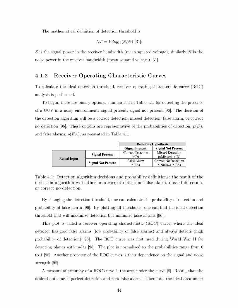
To begin, there are binary options, summarized in Table 4.1, for detecting the presence

of a UUV in a noisy environment: signal present, signal not present [96]. The decision of

the detection algorithm will be a correct detection, missed detection, false alarm, or correct

no detection [96]. These options are representative of the probabilities of detection, 𝑝(𝐷),

and false alarms, 𝑝(𝐹𝐴), as presented in Table 4.1.

Table 4.1: Detection algorithm decisions and probability definitions: the result of thedetection algorithm will either be a correct detection, false alarm, missed detection,or correct no detection.

By changing the detection threshold, one can calculate the probability of detection and

probability of false alarm [96]. By plotting all thresholds, one can find the ideal detection

threshold that will maximize detection but minimize false alarms [96].

This plot is called a receiver operating characteristic (ROC) curve, where the ideal

detector has zero false alarms (low probability of false alarms) and always detects (high

probability of detection) [98]. The ROC curve was first used during World War II for

detecting planes with radar [98]. The plot is normalized so the probabilities range from 0

to 1 [98]. Another property of the ROC curves is their dependence on the signal and noise

strength [98].

A measure of accuracy of a ROC curve is the area under the curve [8]. Recall, that the

desired outcome is perfect detection and zero false alarms. Therefore, the ideal area under

44

the curve of a normalized ROC curve is 1. The closer to 1, the more accurate the ROC

curve [8]. The trapezoidal method for estimating the area under the ROC curve was used

in this thesis [11].

In order to find the optimal detection threshold, the distance to the optimal case, a

probability of detection equal to one and a probability of false alarm equal to zero, was

found:

𝑑 =√(1− 𝑠𝑒𝑛𝑠𝑖𝑡𝑖𝑣𝑖𝑡𝑦)2 + (1− 𝑠𝑝𝑒𝑐𝑖𝑓𝑖𝑐𝑖𝑡𝑦)2[8].

The true positive rate, or probability of detection, is also considered the sensitivity of

the detector [8]. Specificity of the detector is the probability of no false alarms; or

𝑆𝑝𝑒𝑐𝑖𝑓𝑖𝑐𝑖𝑡𝑦 = 1− 𝑃 (𝐹𝐴) [8].

This is related to the Youden index which is

𝑌 𝑜𝑢𝑑𝑒𝑛 𝐼𝑛𝑑𝑒𝑥 = 𝑠𝑒𝑛𝑠𝑖𝑡𝑖𝑣𝑖𝑡𝑦 + 𝑠𝑝𝑒𝑐𝑖𝑓𝑖𝑐𝑖𝑡𝑦 − 1

where the higher the Youden index, the better the detection [8].

4.2 Power Spectral Density

To extract the signal of the UUV from background noise, it is important to first understand

the signal distribution in the frequency domain [77]. Expected instantaneous power is defined

as [77]:

𝐸[𝑥2(𝑡)] = 𝑅𝑥𝑥(0) =12𝜋

∫∞−∞ 𝑆𝑥𝑥(𝑗𝜔)𝑑𝜔,

where x(t) is the incoming signal on the hydrophone, 𝑆𝑥𝑥 is the power spectral density (PSD)

of x(t) and the continuous Fourier transform of the autocorrelation function is 𝑅𝑥𝑥 [77]. The

PSD can be estimated with the Einstein-Wiener-Khinchin theorem:

𝑅𝑥𝑥(𝜏) ⇔ 𝑆𝑥𝑥(𝑗𝜔) = lim𝑇→∞12𝑇 𝐸[|𝑋𝑇 (𝑗𝜔)|2] [77].

This theorem comes from taking a windowed function, 𝑤𝑇 (𝑡), applied to the signal, x(t),

so that it is only defined on the period, T :

𝑥𝑇 (𝑡) = 𝑤𝑇 (𝑡)𝑥(𝑡) [77].

45

The energy spectral density (ESD) is defined as

S𝑥𝑥(𝑗𝜔) = |𝑋𝑇 (𝑗𝜔)|2 [77].

After dividing by the period, 2T, the expression becomes a periodogram:

12𝑇 |𝑋𝑇 (𝑗𝜔)|2 [77].

Taking the limit as the period, T, goes to infinity, this result approaches the power

spectral density, resulting in the Einstein-Wiener-Khinchin theorem [77].

This means that for large periods of T, the frequency resolution will improve [77]. By

averaging over many realizations of the random process x(t) for a given period, T, the

estimate of the power spectral density will improve [77].

In this thesis, the power spectral density of a UUV was found by collecting acoustic data

of the vehicle in a quiet pool environment.

4.3 Underway Vehicle Detection

In order to determine the presence of a vehicle in a realistic environment, short-time Fourier

transform was performed, a spectral filter applied, and the energy calculated.

4.3.1 Short-Time Fourier Transform

Since the process of detecting the vehicle is a function of time, discrete Fourier transform

(DFT) was performed on over-lapping short time periods. This is demonstrated in Figure

4-1. The incoming signal, 𝑥(𝑡), is multiplied by a window function, 𝑤(𝑡), so that the signal

is divided into time segments. Following the segmentation of the signal, DFT was applied

to each snapshot.

4.3.2 Energy Calculation

Acoustic energy from the UUV self-generated noise was calculated by taking the integral of

the energy spectral density over all the frequencies [26]:

𝐸 = 12𝜋

∫∞−∞ |𝐹 (𝑗𝜔)|2𝑑𝜔,

where |𝐹 (𝑗𝜔)|2 is the energy spectral density of 𝑓(𝑡) [26].

46

Figure 4-1: Windowing effect on incoming signal 𝑥(𝑡): when a window function, 𝑤(𝑡),is applied to the signal, the signal becomes segmented, which is used for short-timeFourier transform [55].

4.3.3 Spectral Filters

The advantage of applying a spectral filter to an incoming signal is that one can change

the relative amplitude of frequencies that are important – and even eliminate an unwanted

frequency band entirely [78].

Since the vehicle revealed strong narrowband frequencies, two filters were applied to

improve the signal to noise ratio of the UUV: a bandpass filter and the vehicle PSD estimate

as a filter. A bandpass filter is an example of a frequency-selective filter. It will pass a small

range of frequencies, but attenuate the others not specified in that range, as seen in Figure

4-2 [78].

Figure 4-2: Frequency response of ideal low pass filter: frequencies that are passedthrough are between positive and negative 𝑤, frequencies that are eliminated arerepresented by the stop-band [78].

47

The prominent high frequencies found in the PSD estimate of the vehicle were used as

the defining frequencies of the bandpass filter.

The other filter applied to the data is a frequency-shaping filter [78]. Using the PSD esti-

mate over the entire frequency domain as a filter shaped the frequencies of the input signal,

increasing the amplitude of important frequencies of the UUV and diminishing undesired

frequencies of the UUV.

Frequency filters can be conveniently applied to the incoming signal with the multiplication-

convolution property of Fourier transforms [78]. Starting with the signal, 𝑥(𝑡), and the filter,

ℎ(𝑡), the outgoing filtered signal, 𝑦(𝑡), is

𝑦(𝑡) = 𝑥(𝑡) * ℎ(𝑡) [78].

Transforming this into the frequency domain, the expression becomes

𝑌 (𝜔) = 𝑋(𝜔)𝐻(𝜔) [78].

These filtering concepts were effective in increasing the SNR of the vehicle acoustic signal

in the background noise of the Charles River and Jenkins Pond.

4.3.4 Summary

In practice, a short-time Fourier transform was performed on the incoming signal, a filter

was applied to increase the SNR of the vehicle acoustic signature, and energy was calculated

to determine the presence of the vehicle. This is summarized in Figure 4-3.

The ROC curves were produced based off of various detection thresholds. The probability

of detection, 𝑃 (𝐷), and false alarms, 𝑃 (𝐹𝐴), were calculated from an experiment where

the presence of the vehicle was known. Thus the 𝑃 (𝐹𝐴) and 𝑃 (𝐷) were calculated over the

whole experiment run. Ultimately, the ideal detection threshold was found from the ROC

curves.

For future exercises, the calculated ideal detection threshold would be used, but consid-

erations of the target source level, background noise, and distance of target should all be

taken into account as specified in the passive sonar equation.

48

Figure 4-3: Process for producing ROC curves on a moving target: incoming datafrom a hydrophone element is analyzed by applying short-time Fourier transform,spectral filtering, and energy thresholding. The result is compared to the true presenceof the UUV to calculate probabilities of false alarms and true detections.

4.4 Beamforming

The second part of the analysis involves tracking the direction of arrival of the UUV self-

generated noise. This is accomplished through beamforming, over time, on a horizontal line

array. This section begins by describing beamforming of a single time snapshot of data. The

following section describes the process for performing beamforming over time.

4.4.1 Uniform Linear Arrays

The purpose of an array is to filter signals in the space-time field by finding their spatial

characteristics [94]. These characteristics are a function of an angle or wavenumber, where

wavenumber is defined as

�� = −2𝜋

𝜆

⎡⎢⎢⎢⎢⎣sin(𝜃) cos(𝜑)

sin(𝜃) sin(𝜑)

cos(𝜃)

⎤⎥⎥⎥⎥⎦in the domain pictured in Figure 4-4.

Line arrays, as used in this thesis, resolve angle in only one direction [94]. When there

is equal distance spacing of elements on a line array, this is called a "uniform linear array,"

pictured in Figure 4-5 [94].

49

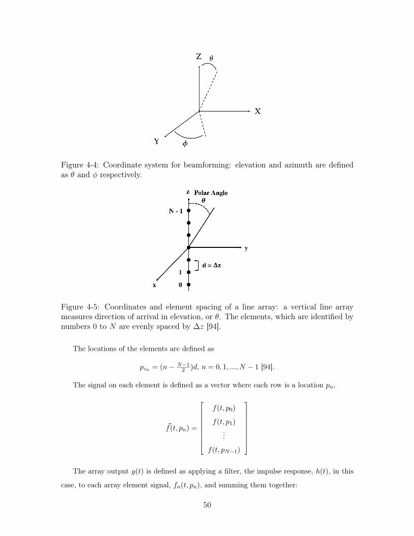
Figure 4-4: Coordinate system for beamforming: elevation and azimuth are definedas 𝜃 and 𝜑 respectively.

Figure 4-5: Coordinates and element spacing of a line array: a vertical line arraymeasures direction of arrival in elevation, or 𝜃. The elements, which are identified bynumbers 0 to 𝑁 are evenly spaced by ∆𝑧 [94].

The locations of the elements are defined as

𝑝𝑧𝑛 = (𝑛− 𝑁−12 )𝑑, 𝑛 = 0, 1, ..., 𝑁 − 1 [94].

The signal on each element is defined as a vector where each row is a location 𝑝𝑛,

𝑓(𝑡, 𝑝𝑛) =

⎡⎢⎢⎢⎢⎢⎢⎢⎣

𝑓(𝑡, 𝑝0)

𝑓(𝑡, 𝑝1)...

𝑓(𝑡, 𝑝𝑁−1)

⎤⎥⎥⎥⎥⎥⎥⎥⎦The array output 𝑦(𝑡) is defined as applying a filter, the impulse response, ℎ(𝑡), in this

case, to each array element signal, 𝑓𝑛(𝑡, 𝑝𝑛), and summing them together:

50

𝑦(𝑡) = Σ𝑁−1𝑛=0

∫∞−∞ ℎ𝑛(𝑡− 𝜏)𝑓𝑛(𝜏, 𝑝𝑛)𝑑𝜏

This order of operations is presented in visual form in Figure 4-6.

Figure 4-6: Filtering process of an array in visual form: the incoming signal on eachelement of the array 𝑓(𝑡, 𝑝𝑛) is filtered by ℎ𝑛(𝜏) and summed together to produce thearray output 𝑦(𝑡) [94].

The array output can also be written compactly in the frequency domain with vectors:

𝑌 (𝜔) = ��𝑇 (𝜔)𝐹 (𝜔)

where

��(𝜔) =∫∞−∞ ℎ(𝑡)𝑒−𝑗𝜔𝑡𝑑𝑡,

and

𝐹 (𝜔, 𝑝) =∫∞−∞ 𝑓(𝑡, 𝑝)𝑒−𝑗𝜔𝑡𝑑𝑡[94].

For a plane wave input, the delay, 𝜏 , between the elements of the array is a function of their

spatial dependence,

𝑓(𝑡, 𝑝) =

⎡⎢⎢⎢⎢⎢⎢⎢⎣

𝑓(𝑡− 𝜏0)

𝑓(𝑡− 𝜏1)...

𝑓(𝑡− 𝜏𝑁−1)

⎤⎥⎥⎥⎥⎥⎥⎥⎦where

𝜏𝑛 = ��𝑇 𝑝𝑛𝑐 [94].

51

In three dimensions, the direction vector, ��, is

�� =

⎡⎢⎢⎢⎢⎣-sin(𝜃) cos(𝜑)

-sin(𝜃) sin(𝜑)

-cos(𝜃)

⎤⎥⎥⎥⎥⎦but in the case of a vertical line array, as pictured in Figure 4-5,

𝑎 = 𝑐𝑜𝑠(𝜃).

The 𝑛𝑡ℎ component of 𝐹 (𝜔) is

𝐹𝑛(𝜔) = 𝑒−𝑗𝜔𝜏𝑛𝐹 (𝜔),

which is a function of the original signal multiplied by a complex exponential of the delay

[94].

Next, the delay is rewritten in terms of the wavenumber

𝜔𝜏𝑛 = ��𝑇 𝑝𝑛,

where the wavenumber is

𝑘 = −2𝜋𝜆 𝑐𝑜𝑠(𝜃) [94].

The incoming signal on the array can then be written in terms of an array manifold

vector,

��𝑘(��) =

⎡⎢⎢⎢⎢⎢⎢⎢⎣

𝑒−𝑗��𝑇 𝑝0

𝑒−𝑗��𝑇 𝑝1

...

𝑒−𝑗��𝑇 𝑝𝑁−1

⎤⎥⎥⎥⎥⎥⎥⎥⎦so it simplifies to

𝐹𝜔 = 𝐹 (𝜔)��𝑘(��).

Finally, a common delay is applied to each element. This process, called "conventional

beamforming" or "delay-and-sum beamforming," is depicted in Figure 4-7 [94].

The filter is

52

Figure 4-7: Delay and sum beamforming process in visual form: the signal on eachelement of the array, 𝑓(𝑡 − 𝜏𝑛), is filtered by applying a delay, ℎ𝑛(𝜏), and summedtogether to produce the array output 𝑦(𝑡) [94].

ℎ𝑛(𝜏) =1𝑁 𝛿(𝜏 + 𝜏𝑛) [94].

The beamforming process can be written more compactly as

��𝑇 (𝜔) = 1𝑁 𝑣𝑘

𝐻(𝑘𝑠)

where 𝑘𝑠 is the desired steering angle [94]. Putting it altogether, the array response is, in

the frequency domain,

𝑌 (𝜔, ��) = ��𝑇 (𝜔)𝑣𝑘(��),

also known as the frequency-wavenumber response function.

In the situation where the signal is narrowband, the delay is actually a phase shift.

Therefore, the gain and phase shift as shown in Figure 4-8, can be adjusted to achieve an

optimal beamformer.

Figure 4-8: Weights for a narrowband beamformer: gain and phase can be modifiedto create an optimal beamformer [94].

The complex weight vector that acts as the gain and phase shifter is

53

��𝐻 = [𝑤*0 𝑤*

1 ... 𝑤*𝑁−1],

so that the frequency wavenumber response is

𝑌 (𝜔, ��) = ��𝐻𝑣𝑘(𝑘)

and

��𝐻 = ��𝑇 (𝜔𝐶) [94].

To transform the frequency-wavenumber function into a beampattern, the wavenumber

is put into terms of an angle that only exists on the visible spectrum. For a uniform linear

array this is

𝐵𝜃(𝜃) = ��𝐻𝑣𝜃(𝜃) = 𝑒−𝑗(𝑁−12

) 2𝜋𝑑𝜆

𝑐𝑜𝑠(𝜃)Σ𝑁−1𝑛=0 𝑤

*𝑛𝑒

𝑗𝑛 2𝜋𝑑𝜆

𝑐𝑜𝑠(𝜃)

with

0 ≤ 𝜃 ≤ 𝜋 [94].

4.4.2 Weighted Linear Arrays

Optimizing the weights of a beampattern can improve the beampattern by narrowing the

beamwidth or decreasing the side lobes.

Uniform Weighting

In the uniform weighting case, seen in Figure 4-9, the weights are

𝑤𝑛 = 1𝑁 , 𝑛 = 0, 1, ...𝑁 − 1

and the beampattern is

𝐵𝜃 =1𝑁

𝑠𝑖𝑛(𝑁2

2𝜋𝜆𝑐𝑜𝑠(𝜃)𝑑)

𝑠𝑖𝑛( 12

2𝜋𝜆𝑐𝑜𝑠(𝜃𝑑))

,

with

0 ≤ 𝜃 ≤ 𝜋 [94].

For uniformly weighted linear arrays, the null-to-null beamwidth, 𝐵𝑊𝑁𝑁 , is

𝐵𝑊𝑁𝑁 = 2 𝜆𝑁𝑑 [94].

54

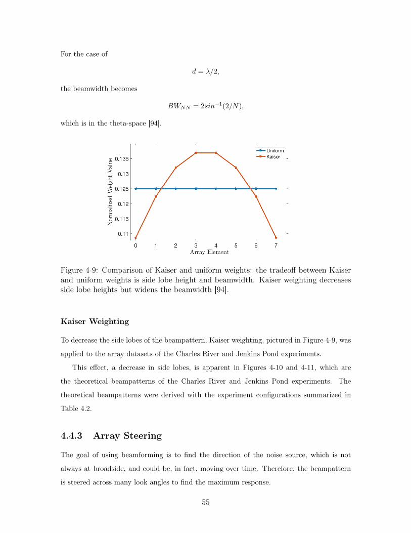
For the case of

𝑑 = 𝜆/2,

the beamwidth becomes

𝐵𝑊𝑁𝑁 = 2𝑠𝑖𝑛−1(2/𝑁),

which is in the theta-space [94].

Figure 4-9: Comparison of Kaiser and uniform weights: the tradeoff between Kaiserand uniform weights is side lobe height and beamwidth. Kaiser weighting decreasesside lobe heights but widens the beamwidth [94].

Kaiser Weighting

To decrease the side lobes of the beampattern, Kaiser weighting, pictured in Figure 4-9, was

applied to the array datasets of the Charles River and Jenkins Pond experiments.

This effect, a decrease in side lobes, is apparent in Figures 4-10 and 4-11, which are

the theoretical beampatterns of the Charles River and Jenkins Pond experiments. The

theoretical beampatterns were derived with the experiment configurations summarized in

Table 4.2.

4.4.3 Array Steering

The goal of using beamforming is to find the direction of the noise source, which is not

always at broadside, and could be, in fact, moving over time. Therefore, the beampattern

is steered across many look angles to find the maximum response.

55

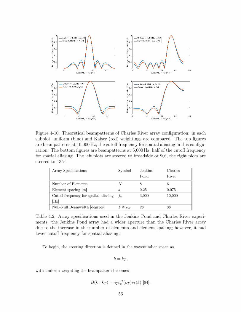
Figure 4-10: Theoretical beampatterns of Charles River array configuration: in eachsubplot, uniform (blue) and Kaiser (red) weightings are compared. The top figuresare beampatterns at 10,000Hz, the cutoff frequency for spatial aliasing in this configu-ration. The bottom figures are beampatterns at 5,000Hz, half of the cutoff frequencyfor spatial aliasing. The left plots are steered to broadside or 90𝑜, the right plots aresteered to 135𝑜.

Array Specifications Symbol JenkinsPond

CharlesRiver

Number of Elements 𝑁 8 6Element spacing [m] 𝑑 0.25 0.075Cutoff frequency for spatial aliasing[Hz]

𝑓𝑐 3,000 10,000

Null-Null Beamwidth [degrees] 𝐵𝑊𝑁𝑁 28 38

Table 4.2: Array specifications used in the Jenkins Pond and Charles River experi-ments: the Jenkins Pond array had a wider aperture than the Charles River arraydue to the increase in the number of elements and element spacing; however, it hadlower cutoff frequency for spatial aliasing.

To begin, the steering direction is defined in the wavenumber space as

𝑘 = 𝑘𝑇 ,

with uniform weighting the beampattern becomes

𝐵(𝑘 : 𝑘𝑇 ) =1𝑁 𝑣𝐻𝑘 (𝑘𝑇 )𝑣𝑘(𝑘) [94].

56

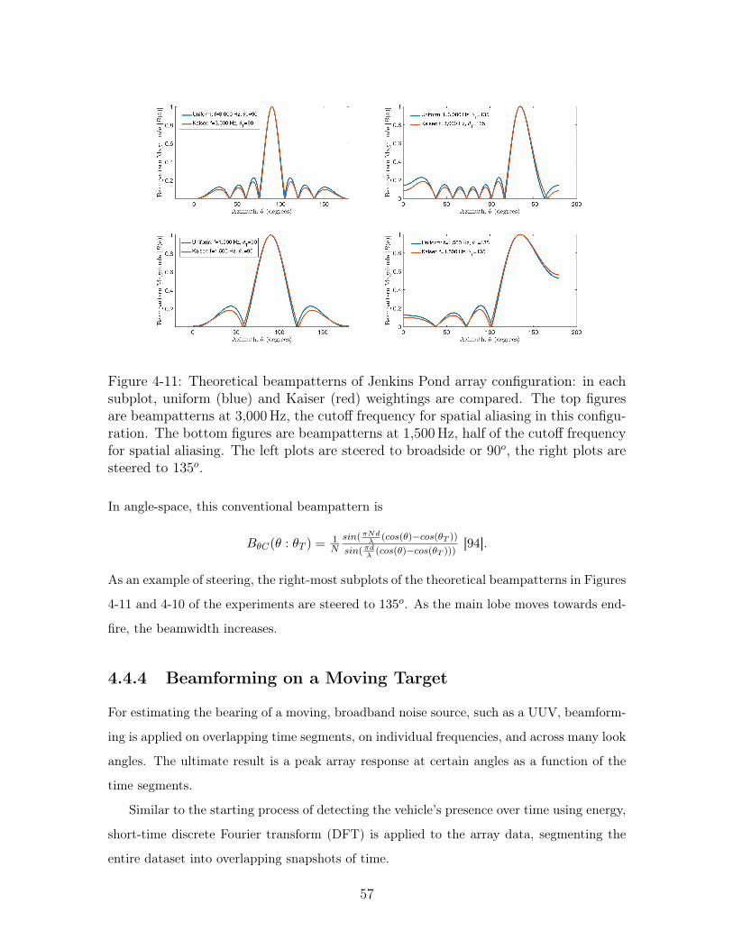
Figure 4-11: Theoretical beampatterns of Jenkins Pond array configuration: in eachsubplot, uniform (blue) and Kaiser (red) weightings are compared. The top figuresare beampatterns at 3,000Hz, the cutoff frequency for spatial aliasing in this configu-ration. The bottom figures are beampatterns at 1,500Hz, half of the cutoff frequencyfor spatial aliasing. The left plots are steered to broadside or 90𝑜, the right plots aresteered to 135𝑜.

In angle-space, this conventional beampattern is

𝐵𝜃𝐶(𝜃 : 𝜃𝑇 ) =1𝑁

𝑠𝑖𝑛(𝜋𝑁𝑑𝜆

(𝑐𝑜𝑠(𝜃)−𝑐𝑜𝑠(𝜃𝑇 ))

𝑠𝑖𝑛(𝜋𝑑𝜆(𝑐𝑜𝑠(𝜃)−𝑐𝑜𝑠(𝜃𝑇 )))

[94].

As an example of steering, the right-most subplots of the theoretical beampatterns in Figures

4-11 and 4-10 of the experiments are steered to 135𝑜. As the main lobe moves towards end-

fire, the beamwidth increases.

4.4.4 Beamforming on a Moving Target

For estimating the bearing of a moving, broadband noise source, such as a UUV, beamform-

ing is applied on overlapping time segments, on individual frequencies, and across many look

angles. The ultimate result is a peak array response at certain angles as a function of the

time segments.

Similar to the starting process of detecting the vehicle’s presence over time using energy,

short-time discrete Fourier transform (DFT) is applied to the array data, segmenting the

entire dataset into overlapping snapshots of time.

57

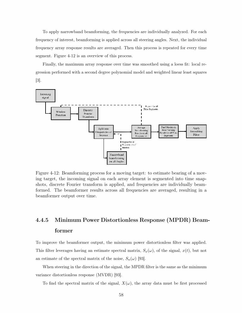
To apply narrowband beamforming, the frequencies are individually analyzed. For each

frequency of interest, beamforming is applied across all steering angles. Next, the individual

frequency array response results are averaged. Then this process is repeated for every time

segment. Figure 4-12 is an overview of this process.

Finally, the maximum array response over time was smoothed using a loess fit: local re-

gression performed with a second degree polynomial model and weighted linear least squares

[3].

Figure 4-12: Beamforming process for a moving target: to estimate bearing of a mov-ing target, the incoming signal on each array element is segmented into time snap-shots, discrete Fourier transform is applied, and frequencies are individually beam-formed. The beamformer results across all frequencies are averaged, resulting in abeamformer output over time.

4.4.5 Minimum Power Distortionless Response (MPDR) Beam-

former

To improve the beamformer output, the minimum power distortionless filter was applied.

This filter leverages having an estimate spectral matrix, 𝑆𝑥(𝜔), of the signal, 𝑥(𝑡), but not

an estimate of the spectral matrix of the noise, 𝑆𝑛(𝜔) [93].

When steering in the direction of the signal, the MPDR filter is the same as the minimum

variance distortionless response (MVDR) [93].

To find the spectral matrix of the signal, 𝑋(𝜔), the array data must be first processed

58

using the time-snapshot model used in detection and conventional beamforming. The signal

is segmented by periods of Δ𝑇 so that its Fourier transform is defined as

𝑋Δ𝑇 (𝜔𝑚) = 1√Δ𝑇

∫Δ𝑇0 𝑥(𝑡)𝑒−𝑗(𝜔𝑐+𝑚𝜔Δ)𝑡𝑑𝑡

where

𝜔𝑚 = 𝜔𝑐 +𝑚𝜔Δ

is the centered frequency with Δ𝜔 frequency resolution, and

𝜔Δ = 2𝜋Δ𝑇

is a function of the snapshot length, Δ𝑇 [92].

The covariance matrix is

𝑆𝑋,Δ𝑇 = 𝐸[𝑋Δ𝑇 (𝜔𝑚)𝑋𝐻Δ𝑇 (𝜔𝑚)].

From the Wiener-Khinchin theorem, for long snapshot periods, Δ𝑇 , the true spectral matrix

of the process can be estimated with the snapshot model:

limΔ𝑇→∞[𝑆𝑥,Δ𝑇 (𝑚,𝑚)]𝑛𝑛 = 𝑆𝑥(𝜔𝑐 +𝑚𝜔Δ𝑇 )]𝑛𝑛 [92].

For a plane-wave signal in noise, like the case of the UUV noise in the ocean, the incoming

signal, 𝑋(𝜔), is broken up by noise and signal:

𝑋(𝜔) = 𝐹 (𝜔)��(𝜔 : 𝑘𝑠) +𝑁(𝜔),

where �� is the array manifold vector, 𝑘𝑠 is the direction of the signal as a wavenumber, 𝐹 (𝜔)

is the source signal of that particular snapshot [93].

The spectral matrix of the noise 𝑁(𝜔) is

𝑆𝑛(𝜔) = 𝑆𝑐 + 𝜎2𝜔𝐼,

where 𝜎2𝜔 is the white noise component. For the total signal and noise, 𝑋(𝜔), the spectral

matrix is

𝑆𝑥(𝜔) = 𝑆𝑓 (𝜔)𝑣(𝜔 : 𝑘𝑠)𝑣𝐻(𝜔 : 𝑘𝑠) + 𝑆𝑛(𝜔),

59

where 𝑆𝑓 (𝜔) is the variance of 𝐹 (𝜔) [93].

Without knowledge of the direction of the desired signal and the noise spectral matrix,

an optimal beamformer – MPDR – can be derived with the spectral matrix of the signal

and noise together, 𝑆𝑥(𝜔), by minimizing the output power of the filter with a distortionless

constraint [93].

The criteria of a distortionless filter, ��𝐻 , is

��𝐻𝑣𝑚=1,

where 𝑣𝑚 is the steering vector in the direction of the signal [93].

The filter result is

𝑤𝑀𝑃𝐷𝑅𝐻 = 𝑣𝑚

𝐻𝑆−1𝑥

𝑣𝑚𝐻𝑆−1

𝑥 𝑣𝑚[93].

In practice, the estimate of 𝑆𝑥 changes over time by using the process of time snapshots.

As a consequence, 𝑆𝑥 is adaptively optimized to the environment which fluctuates over time.

60

Chapter 5

Experimental Methods

One pool experiment was completed to find the power spectral density of the UUV self-

generated noise and two field experiments were completed to demonstrate tracking a UUV

in a realistic environment.

5.1 Bluefin Sandshark UUV

The Bluefin Sandshark UUV, pictured in Figure 5-1, was used to demonstrate tracking a

UUV in a realistic environment [73].

Figure 5-1: Bluefin Sandshark micro-UUV: this micro-UUV manufactured by BluefinRobotics was used to demonstrate passive detection and tracking in a pond and riverexperiment [73].

The Bluefin Sandshark is in the micro-size category of UUVs due to its compact size of

approximately 15 lbs. The vehicle is torpedo-shaped, with a single propeller. An overview

of its manufacturer specifications is in Table 5.1

The estimated position outputted by the inertial navigation system (INS) of the vehicle

61

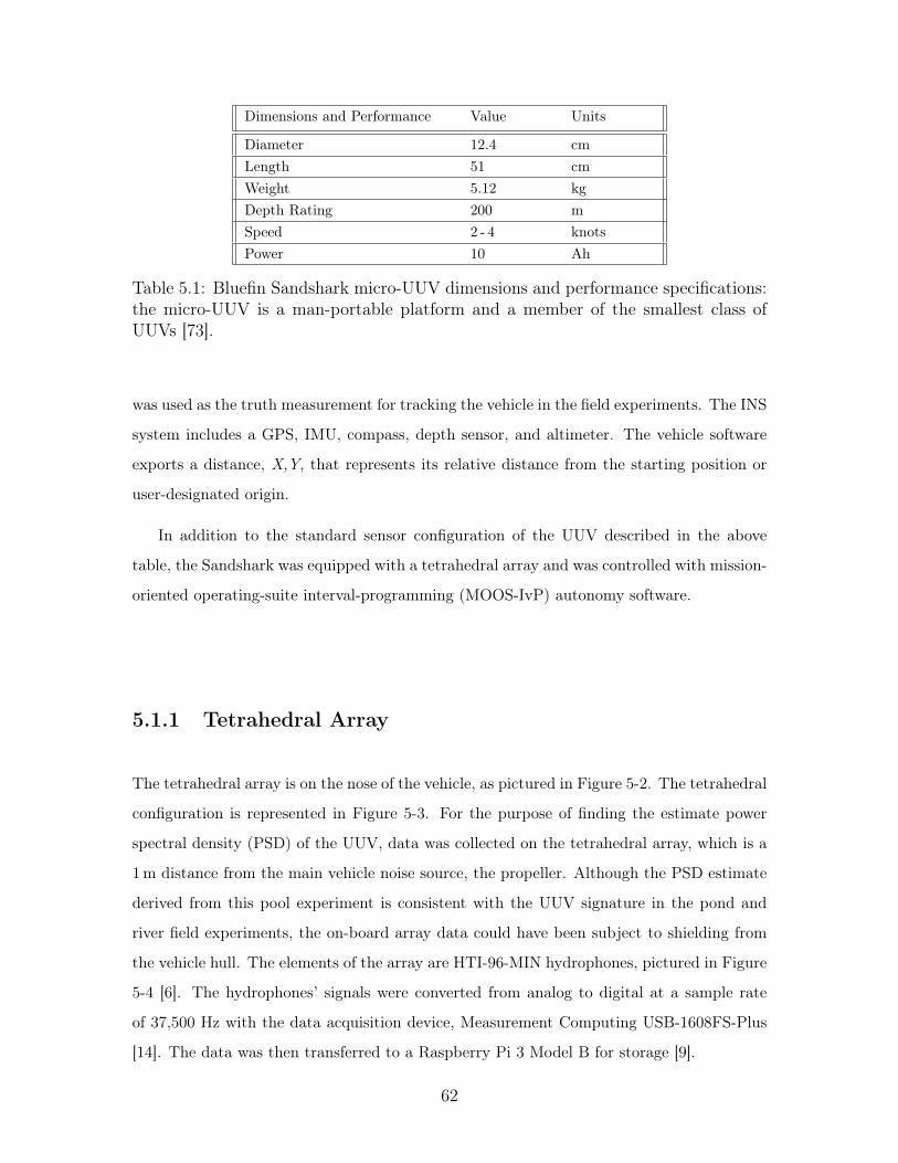
Dimensions and Performance Value Units

Diameter 12.4 cmLength 51 cmWeight 5.12 kgDepth Rating 200 mSpeed 2 - 4 knotsPower 10 Ah

Table 5.1: Bluefin Sandshark micro-UUV dimensions and performance specifications:the micro-UUV is a man-portable platform and a member of the smallest class ofUUVs [73].

was used as the truth measurement for tracking the vehicle in the field experiments. The INS

system includes a GPS, IMU, compass, depth sensor, and altimeter. The vehicle software

exports a distance, X,Y, that represents its relative distance from the starting position or

user-designated origin.

In addition to the standard sensor configuration of the UUV described in the above

table, the Sandshark was equipped with a tetrahedral array and was controlled with mission-

oriented operating-suite interval-programming (MOOS-IvP) autonomy software.

5.1.1 Tetrahedral Array

The tetrahedral array is on the nose of the vehicle, as pictured in Figure 5-2. The tetrahedral

configuration is represented in Figure 5-3. For the purpose of finding the estimate power

spectral density (PSD) of the UUV, data was collected on the tetrahedral array, which is a

1 m distance from the main vehicle noise source, the propeller. Although the PSD estimate

derived from this pool experiment is consistent with the UUV signature in the pond and

river field experiments, the on-board array data could have been subject to shielding from

the vehicle hull. The elements of the array are HTI-96-MIN hydrophones, pictured in Figure

5-4 [6]. The hydrophones’ signals were converted from analog to digital at a sample rate

of 37,500 Hz with the data acquisition device, Measurement Computing USB-1608FS-Plus

[14]. The data was then transferred to a Raspberry Pi 3 Model B for storage [9].

62

Figure 5-2: Tetrahedral array in nose payload section of the Bluefin Sandshark micro-UUV.

Figure 5-3: Element configuration of a tetrahedral array: a tetrahedral array is in thenose payload section of the micro-UUV, which was used to collect acoustic data forthe PSD estimate of the vehicle.

5.1.2 Autonomy – MOOS-IvP

In order for the vehicle to follow a loiter pattern autonomously, MOOS-IvP autonomy soft-

ware was utilized to control the behavior of the vehicle. MOOS-IvP is open-source au-

tonomous software designed for maritime platforms like UUVs [5]. The software is main-

tained by MIT and the Oxford Robotics Institute [5].

At a high level, the autonomy decision-making process follows a front seat, back seat

configuration [5]. The front seat is defined as the internal vehicle controls and the back

seat is run by MOOS-IvP which makes the intelligent autonomous decisions during the

mission [5]. The two controllers work together by sharing information [5]. The main vehicle

computer sends vehicle state information, including current speed and position [5]. In turn,

the autonomy board sends desired speed, heading, and position [5]. This flow of information

is represented in Figure 5-5.

63

Figure 5-4: Hydrophone element HTI-96-MIN: this hydrophone was used to measurethe power spectral density estimate of the micro-UUV. Four of the hydrophones areconfigured in a tetrahedral array in the nose of the Bluefin Sandshark micro-UUVused in these experiments [6].

Figure 5-5: Autonomy decision-making process of MOOS-IvP software: MOOS-IvPis configured such that the vehicle computer is separate from the autonomy payload[5].

5.2 Horizontal Line Array

The estimated bearing of the Sandshark UUV was accomplished through beamforming on a

horizontal line array. In the experiments, the horizontal line array consisted of six (Charles

River) and eight (Jenkins Pond) HTI-96-MIN hydrophone elements [6]. Modeled after the

setup in the tetrahedral array, the analog hydrophone signals are converted to a digital

signal through the data acquisition system, Measurement Computing USB-1608FS-Plus, at

a sampling rate of 19,200 Hz (Jenkins Pond experiment) or 37,500 Hz (Charles River) [14].

Then the data is stored on a Raspberry Pi 3 Model B for future processing [9]. A summary

of the transfer of data on the horizontal line array is shown in Figure 5-6.

5.3 Power Spectral Density Estimate – Test Setup

The power spectral density (PSD) experiment with the Sandshark micro-UUV took place

at the MIT alumni pool on February 2, 2017. The pool, pictured in Figure 5-7, was chosen

for being isolated from outside noise sources. The MIT pool dimensions are 20 ft by 40 ft

64

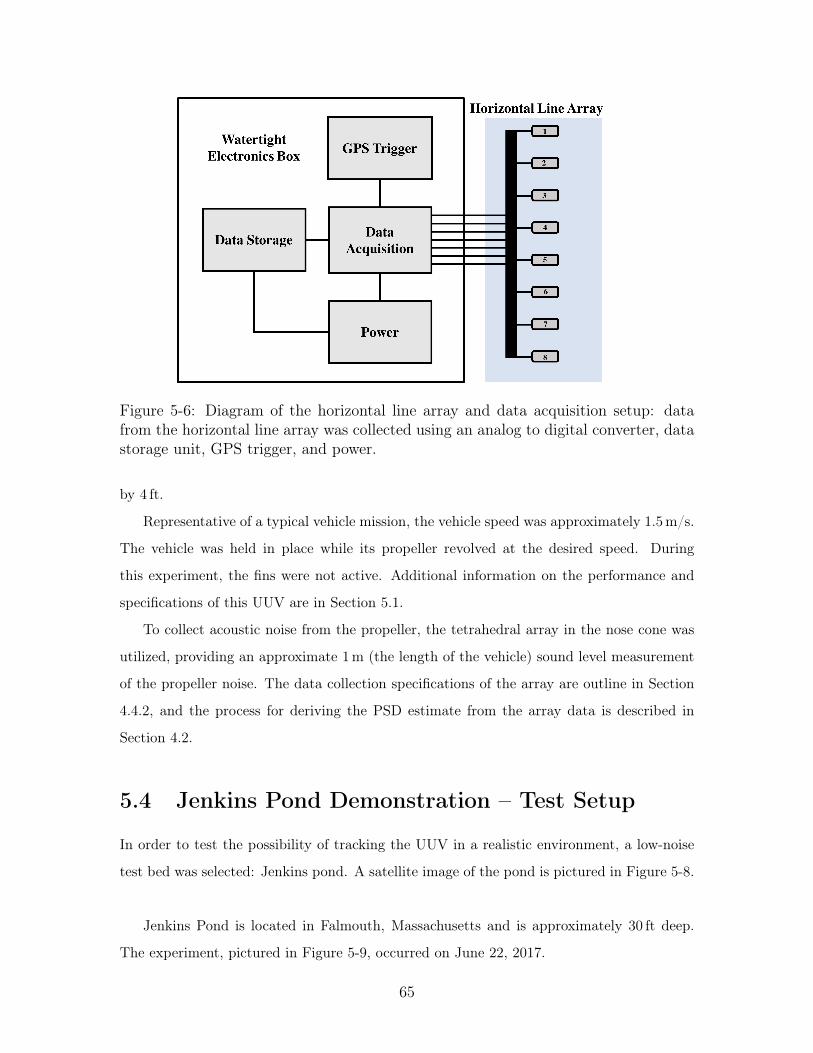
Figure 5-6: Diagram of the horizontal line array and data acquisition setup: datafrom the horizontal line array was collected using an analog to digital converter, datastorage unit, GPS trigger, and power.

by 4 ft.

Representative of a typical vehicle mission, the vehicle speed was approximately 1.5m/s.

The vehicle was held in place while its propeller revolved at the desired speed. During

this experiment, the fins were not active. Additional information on the performance and

specifications of this UUV are in Section 5.1.

To collect acoustic noise from the propeller, the tetrahedral array in the nose cone was

utilized, providing an approximate 1 m (the length of the vehicle) sound level measurement

of the propeller noise. The data collection specifications of the array are outline in Section

4.4.2, and the process for deriving the PSD estimate from the array data is described in

Section 4.2.

5.4 Jenkins Pond Demonstration – Test Setup

In order to test the possibility of tracking the UUV in a realistic environment, a low-noise

test bed was selected: Jenkins pond. A satellite image of the pond is pictured in Figure 5-8.

Jenkins Pond is located in Falmouth, Massachusetts and is approximately 30 ft deep.

The experiment, pictured in Figure 5-9, occurred on June 22, 2017.

65

Figure 5-7: Power spectral density estimate experiment at the MIT alumni pool: theBluefin Sandshark micro-UUV was secured while its propellor revolved at approxi-mately 1.5m/s. The onboard acoustic sensors collected acoustic noise data.

The Bluefin Sandshark UUV was used for this experiment and was programmed with

MOOS-IvP to follow a loiter behavior. The details of the equipment and autonomy software

are in Section 5.1 and Section 5.1.2. Figure 5-10 shows an overview of the vehicle track over

time (the colorbar). The vehicle travelled approximately 70 m away from the beach where

the horizontal line array was mounted. The depth and speed of the vehicle are shown in

Figures 5-11 and 5-12 respectively. The overall vehicle speed was 1.5 m/s while it travelled

closely to the surface at 0.5 m depth. This navigation data was produced by the vehicle’s

inertial navigation system. In post-processing, this data is used as the true position of the

vehicle, a benchmark for the estimated bearing from the horizontal line array (HLA). The

resurfacing behavior to achieve a GPS fix is shown by the periodic zero-depth and zero-speed

of the vehicle.

The HLA was bottom mounted near the starting point of the vehicle at (-40,-60). Data

from the array was collected and analyzed post-experiment to derive an estimated bearing

and detect the presence of the UUV.

66

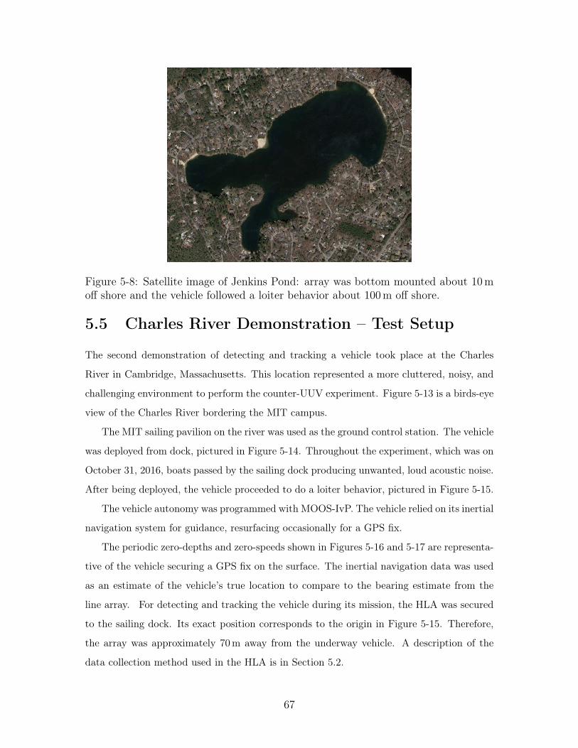
Figure 5-8: Satellite image of Jenkins Pond: array was bottom mounted about 10moff shore and the vehicle followed a loiter behavior about 100m off shore.

5.5 Charles River Demonstration – Test Setup

The second demonstration of detecting and tracking a vehicle took place at the Charles

River in Cambridge, Massachusetts. This location represented a more cluttered, noisy, and

challenging environment to perform the counter-UUV experiment. Figure 5-13 is a birds-eye

view of the Charles River bordering the MIT campus.

The MIT sailing pavilion on the river was used as the ground control station. The vehicle

was deployed from dock, pictured in Figure 5-14. Throughout the experiment, which was on

October 31, 2016, boats passed by the sailing dock producing unwanted, loud acoustic noise.

After being deployed, the vehicle proceeded to do a loiter behavior, pictured in Figure 5-15.

The vehicle autonomy was programmed with MOOS-IvP. The vehicle relied on its inertial

navigation system for guidance, resurfacing occasionally for a GPS fix.

The periodic zero-depths and zero-speeds shown in Figures 5-16 and 5-17 are representa-

tive of the vehicle securing a GPS fix on the surface. The inertial navigation data was used

as an estimate of the vehicle’s true location to compare to the bearing estimate from the

line array. For detecting and tracking the vehicle during its mission, the HLA was secured

to the sailing dock. Its exact position corresponds to the origin in Figure 5-15. Therefore,

the array was approximately 70 m away from the underway vehicle. A description of the

data collection method used in the HLA is in Section 5.2.

67

Figure 5-9: Shore launch of vehicle at Jenkins pond: the UUV was launched from theshore and the array was bottom mounted about 10m from the shoreline.

Figure 5-10: UUV track in X-Y coordinates over time at the Jenkins Pond experiment:UUV performed a loiter pattern about 100 m offshore. The progression of time isrepresented by the colorbar and the total mission time was about 20min. Navigationdata was taken from the vehicle’s inertial navigation system.

68

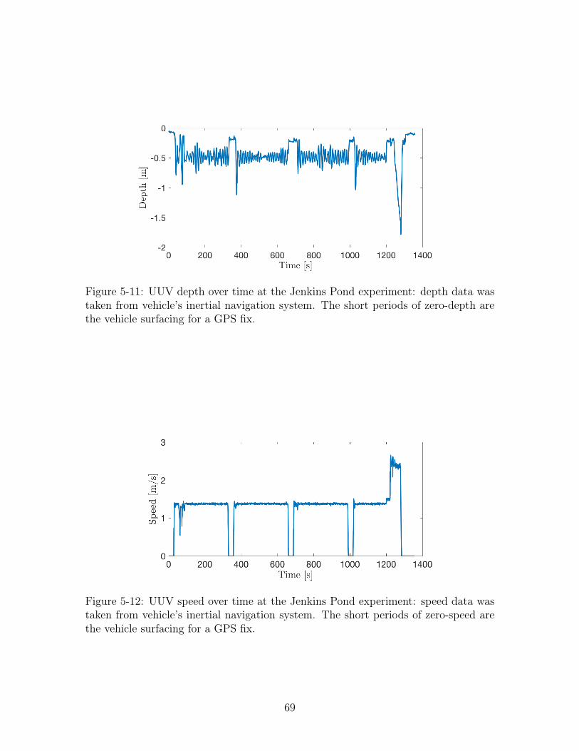
Figure 5-11: UUV depth over time at the Jenkins Pond experiment: depth data wastaken from vehicle’s inertial navigation system. The short periods of zero-depth arethe vehicle surfacing for a GPS fix.

Figure 5-12: UUV speed over time at the Jenkins Pond experiment: speed data wastaken from vehicle’s inertial navigation system. The short periods of zero-speed arethe vehicle surfacing for a GPS fix.

69

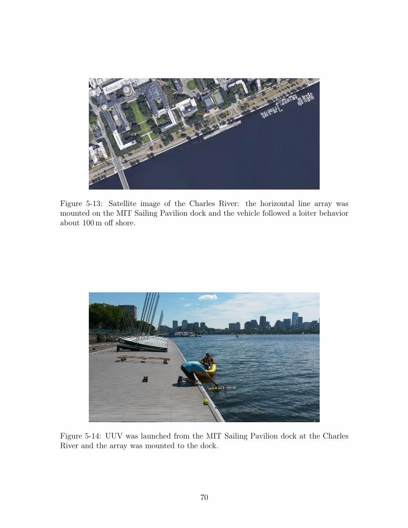
Figure 5-13: Satellite image of the Charles River: the horizontal line array wasmounted on the MIT Sailing Pavilion dock and the vehicle followed a loiter behaviorabout 100 m off shore.

Figure 5-14: UUV was launched from the MIT Sailing Pavilion dock at the CharlesRiver and the array was mounted to the dock.

70

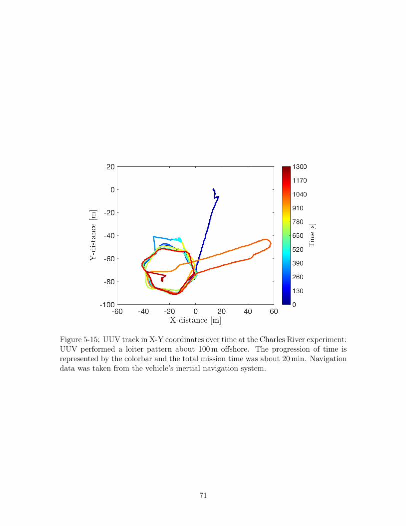
Figure 5-15: UUV track in X-Y coordinates over time at the Charles River experiment:UUV performed a loiter pattern about 100m offshore. The progression of time isrepresented by the colorbar and the total mission time was about 20min. Navigationdata was taken from the vehicle’s inertial navigation system.

71

Figure 5-16: UUV depth over time at the Charles River experiment: depth data wastaken from vehicle’s inertial navigation system. The short periods of zero-depth arethe vehicle surfacing for a GPS fix.

Figure 5-17: UUV speed over time at the Charles River experiment: speed data wastaken from vehicle’s inertial navigation system. The short periods of zero-speed arethe vehicle surfacing for a GPS fix.

72

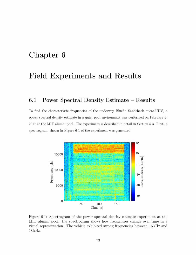
Chapter 6

Field Experiments and Results

6.1 Power Spectral Density Estimate – Results

To find the characteristic frequencies of the underway Bluefin Sandshark micro-UUV, a

power spectral density estimate in a quiet pool environment was performed on February 2,

2017 at the MIT alumni pool. The experiment is described in detail in Section 5.3. First, a

spectrogram, shown in Figure 6-1 of the experiment was generated.

Figure 6-1: Spectrogram of the power spectral density estimate experiment at theMIT alumni pool: the spectrogram shows how frequencies change over time in avisual representation. The vehicle exhibited strong frequencies between 16 kHz and18 kHz.

73

This visual representation of the experiment shows the strength of certain frequencies

over time. The spectrogram is created by taking the discrete Fourier transform (DFT) of

overlapping time segments. The most interesting component of this result is the strong

high frequencies of the vehicle between 16 kHz and 18 kHz. For this dataset, however, the

sampling frequency, 𝑓𝑠, was 37,500Hz. As a consequence, the strong frequencies between

16 kHz and 18 kHz were actually aliased, and the true frequency, 𝑓𝑡𝑟𝑢𝑒, is between 19,500 Hz

and 21,500 Hz:

𝑓𝑎𝑙𝑖𝑎𝑠𝑒𝑑 = |𝑓𝑡𝑟𝑢𝑒 − 𝑓𝑠|.

This aliasing effect is consistent with the in-water tests of Jenkins Pond and the Charles

River.

Secondly, the overall increase in acoustic power at approximately 25 s and 175 s can be

observed when the vehicle is turned on and off.

To derive the PSD, the magnitude of each realization, or DFT of the time snapshot,

was found, squared, and averaged over all the realizations. The normalized PSD result is in

Figure 6-2. The mean and standard deviation are both plotted to show the magnitude of the

Figure 6-2: Power spectral density estimate of Bluefin Sandshark micro-UUV: thepower spectral density estimate was derived from acoustic data collected on-boardthe vehicle. The data was collected in a pool environment. The standard deviationof the data was used as the error margin.

variance of power over time. This is to be expected because of the random characteristics of

broadband propeller noise. Again, as seen in the spectrogram, the high frequencies between

16 kHz and 18 kHz are the most identifying, prominent frequencies of the underway vehicle.

74

6.2 Jenkins Pond Demonstration – Results

A demonstration of detecting and tracking a vehicle – a Bluefin Sandshark UUV – was

performed at Jenkins Pond in Falmouth, Massachusetts, on June 22, 2017. The pond

represents an environment that a vehicle might encounter on an ISR mission in littoral

waters. The vehicle loitered about 100m offshore and was picked up and tracked by the

bottom mounted array. Section 5.4 describes the array location, vehicle trajectory, and pond

dimensions in detail.

The signal from a single hydrophone element was first analyzed by applying short-time

Fourier transform and calculating power as a function of frequency. By evaluating the power

of different frequency bands, and how they change over time, one can gain knowledge of the

environmental noise and vehicle signal. Consequently, the vehicle can be identified in the

background noise of the pond – which included foot traffic on the beach, boats passing by,

and multipath effects from the shallow water.

In the case of this experiment, the sampling rate was 19,200 Hz and the spectrogram –

the frequency power over time – pictured in Figure 6-3 has a cutoff frequency of 9,600 Hz.

The vehicle enters the water at about 800 s and is identifiable by its strong frequency around

800 Hz. The vehicle also has strong broadband noise between 3,000 - 4,000 Hz. With the UUV

PSD estimate in mind, the vehicle has a strong frequency at 20,000Hz, which is aliased in

the Jenkins pond dataset to 800Hz.

6.2.1 Detection

Following finding the spectrogram of the experiment, energy across the frequencies was

calculated to detect the presence of the vehicle. To improve detection, a bandpass filter was

also used on the 800Hz, the aliased but identifiable, frequency of the vehicle.

Figure 6-4 is the ROC curve comparison of filter applied and no filter. With no filter, the

probability of detection is 70.4 % and probability of false alarms is 49.4%. With a bandpass

filter on the aliased frequency of 800 Hz, this improves to a probability of detection of 71.0 %

and false alarm rate of 36.0 %. False alarms decreased by 13.5%.

The ROC curve area, presented in Figure 6-5, is a measure of how well the detector

performs. In the case of no filter, the area was 0.61, which is close to 0.5, so it is considered

a very poor detector – 50 % false alarms, 50% true detection. By adding a bandpass filter

75

Figure 6-3: Spectrogram of the Jenkins Pond experiment: the spectrogram shows howfrequencies change over time in a visual representation. The vehicle is identifiable byits strong frequency tone at 800Hz, which is aliased down from the true frequency of20 kHz. The vehicle enters the water at around 800 s.

the area increases to 0.69.

The detection results are compared in Table 6.1, which shows that the filter decreases

the false alarms rates by 13.5 %.

No Filter Bandpass Filter

P(D) 70.4 71.0P(FA) 49.5 36.0

Table 6.1: Probability of detection and false alarms from the ideal detection thresholdfor the Jenkins Pond experiment. The bandpass filter was applied to the aliasedfrequency of 800 Hz.

6.2.2 Tracking

After confirming the presence of the vehicle, in practice, the bearing of the vehicle is tracked

over time – giving insight to the vehicle’s true trajectory and intentions.

In the Jenkins Pond experiment, the vehicle bearing is estimated with a horizontal line

array with specifications outlined in Section 4.4.2. The array was bottom mounted and

about 80 m from the vehicle while it followed a loiter pattern.

76

Figure 6-4: ROC curves from the Jenkins Pond experiment: the bandpass filterapplied to the aliased frequency of 800Hz outperforms no filter applied to the data.

Since the vehicle changed direction over time, the array data was divided into time

snapshots, then DFT and beamforming was carried out on each segment. These results,

with conventional beamforming, are in Figure 6-6. The x-axis is time, showing how the

beamforming results evolve. At each time segment, the beamforming results were averaged

over frequencies, 1000 - 8000 Hz, because of the broadband nature of the vehicle. There is

a broadband interferer at broadside or 90 ∘. This is potentially due to interference on the

beach – like people and boat traffic. Despite this intense interferer, the triangular trajectory

that oscillates between 80 ∘ and 120 ∘ is the true trajectory of the vehicle.

In Figure 6-7, the expected true trajectory of the vehicle is plotted in blue. This was

found using the inertial navigation system and the orientation of the array. The beamforming

results, plotted in red in Figure 6-7, follow the same shape – a triangular function over time

– which correlates to the vehicle pursuing a loiter pattern.

Due to the interferer at broadside, the maximum beamforming results match the shape

but not the exact troughs and peaks of the true trajectory. The expected vehicle bearing,

calculated from the vehicle inertial navigation system, is between 80 ∘ and 115 ∘; instead

the estimated bearing, from the array data, is between 90 ∘ and 105 ∘. The maximum

beamforming results were found by applying a smoothing filter to the maximum beamformer

output described in Section 4.4.4.

For a comparison over time, Figure 6-8 shows the absolute angle difference between

77

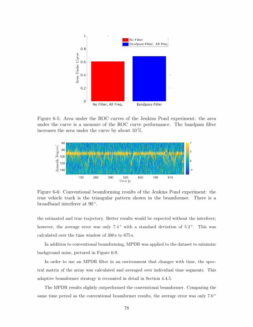
Figure 6-5: Area under the ROC curves of the Jenkins Pond experiment: the areaunder the curve is a measure of the ROC curve performance. The bandpass filterincreases the area under the curve by about 10%.

Figure 6-6: Conventional beamforming results of the Jenkins Pond experiment: thetrue vehicle track is the triangular pattern shown in the beamformer. There is abroadband interferer at 90 ∘.

the estimated and true trajectory. Better results would be expected without the interferer;

however, the average error was only 7.4 ∘ with a standard deviation of 5.2 ∘. This was

calculated over the time window of 380 s to 675 s.

In addition to conventional beamforming, MPDR was applied to the dataset to minimize

background noise, pictured in Figure 6-9.

In order to use an MPDR filter in an environment that changes with time, the spec-

tral matrix of the array was calculated and averaged over individual time segments. This

adaptive beamformer strategy is recounted in detail in Section 4.4.5.

The MPDR results slightly outperformed the conventional beamformer. Comparing the

same time period as the conventional beamformer results, the average error was only 7.0 ∘

78

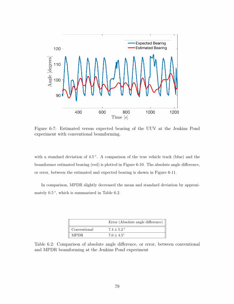
Figure 6-7: Estimated versus expected bearing of the UUV at the Jenkins Pondexperiment with conventional beamforming.

with a standard deviation of 4.5 ∘. A comparison of the true vehicle track (blue) and the

beamformer estimated bearing (red) is plotted in Figure 6-10. The absolute angle difference,

or error, between the estimated and expected bearing is shown in Figure 6-11.

In comparison, MPDR slightly decreased the mean and standard deviation by approxi-

mately 0.5 ∘, which is summarized in Table 6.2.

Error (Absolute angle difference)

Conventional 7.4± 5.2 ∘

MPDR 7.0± 4.5∘

Table 6.2: Comparison of absolute angle difference, or error, between conventionaland MPDR beamforming at the Jenkins Pond experiment

79

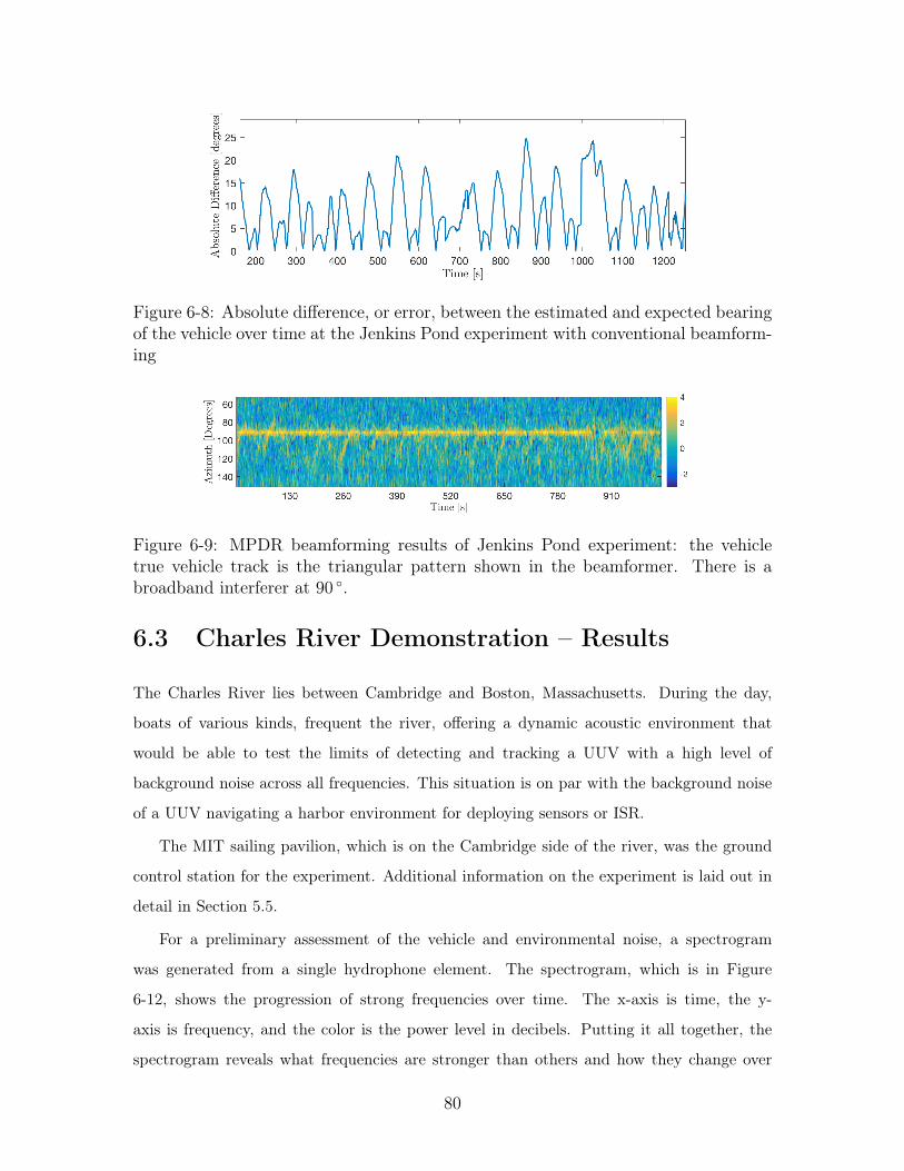
Figure 6-8: Absolute difference, or error, between the estimated and expected bearingof the vehicle over time at the Jenkins Pond experiment with conventional beamform-ing

Figure 6-9: MPDR beamforming results of Jenkins Pond experiment: the vehicletrue vehicle track is the triangular pattern shown in the beamformer. There is abroadband interferer at 90 ∘.

6.3 Charles River Demonstration – Results

The Charles River lies between Cambridge and Boston, Massachusetts. During the day,

boats of various kinds, frequent the river, offering a dynamic acoustic environment that

would be able to test the limits of detecting and tracking a UUV with a high level of

background noise across all frequencies. This situation is on par with the background noise

of a UUV navigating a harbor environment for deploying sensors or ISR.

The MIT sailing pavilion, which is on the Cambridge side of the river, was the ground

control station for the experiment. Additional information on the experiment is laid out in

detail in Section 5.5.

For a preliminary assessment of the vehicle and environmental noise, a spectrogram

was generated from a single hydrophone element. The spectrogram, which is in Figure

6-12, shows the progression of strong frequencies over time. The x-axis is time, the y-

axis is frequency, and the color is the power level in decibels. Putting it all together, the

spectrogram reveals what frequencies are stronger than others and how they change over

80

Figure 6-10: Estimated versus expected bearing of the UUV at the Jenkins Pondexperiment with MPDR beamforming.

time. This spectrogram was created using a 50% overlap of time segments and a sampling

frequency of 37,500Hz.

The vehicle enters the scene at about 300 s and exits at 800 s. The vehicle is identifiable

by a strong tone at 17,500Hz which is actually an aliased frequency of 20 kHz. The vehicle

noise is also apparent by its broadband noise from 2,000 Hz to 8,000Hz.

The broadband short bursts at 50 - 70 s and 650 - 700 s are examples of a boat passing

by. The strong tone that fluctuates between 10 kHz and 12 kHz was present in the entire

dataset. Its origin is unknown, but it could be caused by a loud electronics source on the

boat dock.

6.3.1 Detection

After observing the spectrogram features of the data, detection analysis was performed by

energy thresholding and spectral filtering to detect the vehicle in background noise. The

three filters applied were the power spectral density (PSD) estimate as a filter, across all

81

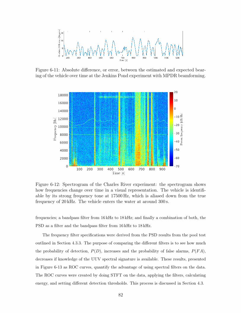
Figure 6-11: Absolute difference, or error, between the estimated and expected bear-ing of the vehicle over time at the Jenkins Pond experiment with MPDR beamforming.

Figure 6-12: Spectrogram of the Charles River experiment: the spectrogram showshow frequencies change over time in a visual representation. The vehicle is identifi-able by its strong frequency tone at 17500Hz, which is aliased down from the truefrequency of 20 kHz. The vehicle enters the water at around 300 s.

frequencies; a bandpass filter from 16 kHz to 18 kHz; and finally a combination of both, the

PSD as a filter and the bandpass filter from 16 kHz to 18 kHz.

The frequency filter specifications were derived from the PSD results from the pool test

outlined in Section 4.3.3. The purpose of comparing the different filters is to see how much

the probability of detection, 𝑃 (𝐷), increases and the probability of false alarms, 𝑃 (𝐹𝐴),

decreases if knowledge of the UUV spectral signature is available. These results, presented

in Figure 6-13 as ROC curves, quantify the advantage of using spectral filters on the data.

The ROC curves were created by doing STFT on the data, applying the filters, calculating

energy, and setting different detection thresholds. This process is discussed in Section 4.3.

82

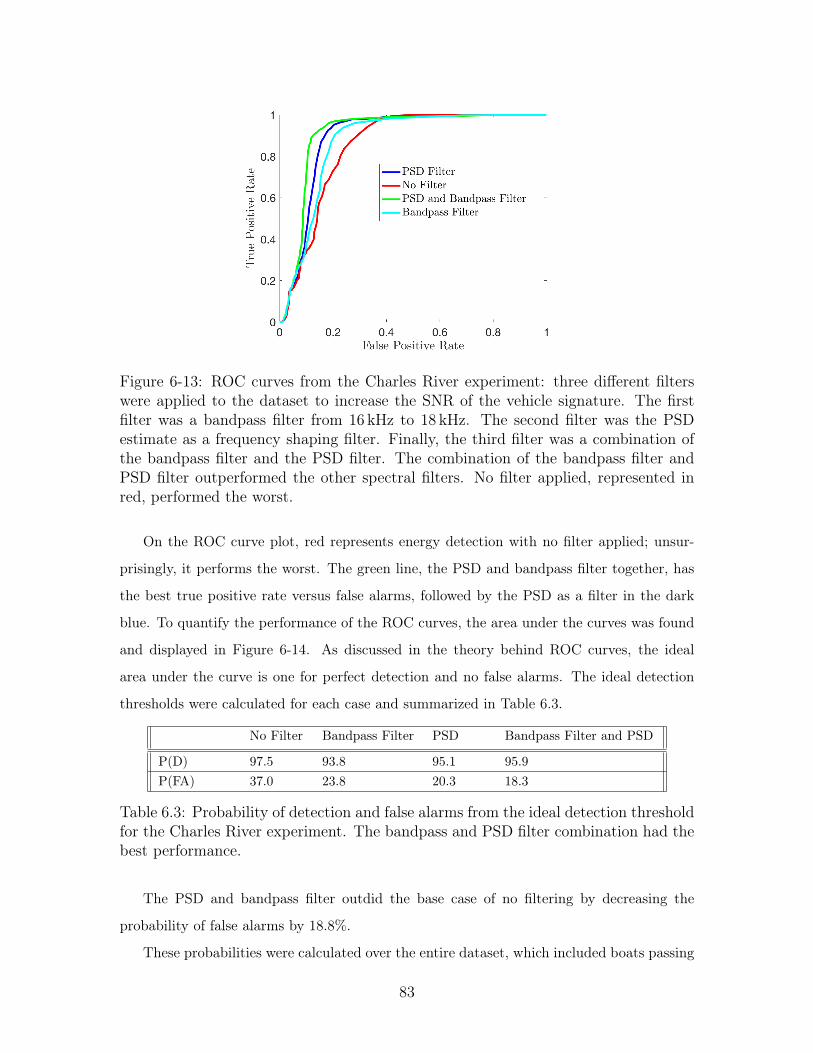
Figure 6-13: ROC curves from the Charles River experiment: three different filterswere applied to the dataset to increase the SNR of the vehicle signature. The firstfilter was a bandpass filter from 16 kHz to 18 kHz. The second filter was the PSDestimate as a frequency shaping filter. Finally, the third filter was a combination ofthe bandpass filter and the PSD filter. The combination of the bandpass filter andPSD filter outperformed the other spectral filters. No filter applied, represented inred, performed the worst.

On the ROC curve plot, red represents energy detection with no filter applied; unsur-

prisingly, it performs the worst. The green line, the PSD and bandpass filter together, has

the best true positive rate versus false alarms, followed by the PSD as a filter in the dark

blue. To quantify the performance of the ROC curves, the area under the curves was found

and displayed in Figure 6-14. As discussed in the theory behind ROC curves, the ideal

area under the curve is one for perfect detection and no false alarms. The ideal detection

thresholds were calculated for each case and summarized in Table 6.3.

No Filter Bandpass Filter PSD Bandpass Filter and PSD

P(D) 97.5 93.8 95.1 95.9P(FA) 37.0 23.8 20.3 18.3

Table 6.3: Probability of detection and false alarms from the ideal detection thresholdfor the Charles River experiment. The bandpass and PSD filter combination had thebest performance.

The PSD and bandpass filter outdid the base case of no filtering by decreasing the

probability of false alarms by 18.8%.

These probabilities were calculated over the entire dataset, which included boats passing

83

Figure 6-14: Area under the ROC curves of the Charles River experiment: the areaunder the curve is a measure of the ROC curve performance. The PSD and bandpassfilter combination increases the area under the curve by about 10% from no filterapplied

by. In the case of a harbor with little activity, it is expected that these detection rates would

be even better. Furthermore, it should be noted that this and the previous experiments were

conducted with the Sandshark micro-UUV, which is the smallest class of vehicles. As vehicles

increase their size, the potential number of sources of electro-mechanical noise also increases

– such as the complexity and size of the propulsion system. The detection results have the

potential to improve on mid- to large-sized vehicles that are more commonly used by navies.

6.3.2 Tracking

Succeeding the detection of the UUV with energy thresholding and spectral filtering, the

vehicle noise source was tracked with a horizontal line array. The array provides an estimate

bearing to the vehicle position which, in practice, could provide situational awareness of a

UUV’s intent to a ship, harbor, or submarine.

In the Charles River experiment, the horizontal line array (HLA) was mounted to the

sailing pavilion dock where the vehicle was initially deployed. Pictures of the setup are

provided in Section 5.5.

The HLA consisted of six elements with a spacing of 0.075m and a temporal sampling

frequency of 37,500 Hz. As outlined in Section 4.4.4, the array data was segmented into

overlapping time snapshots. Then DFT was applied and this result was beamformed, and

84

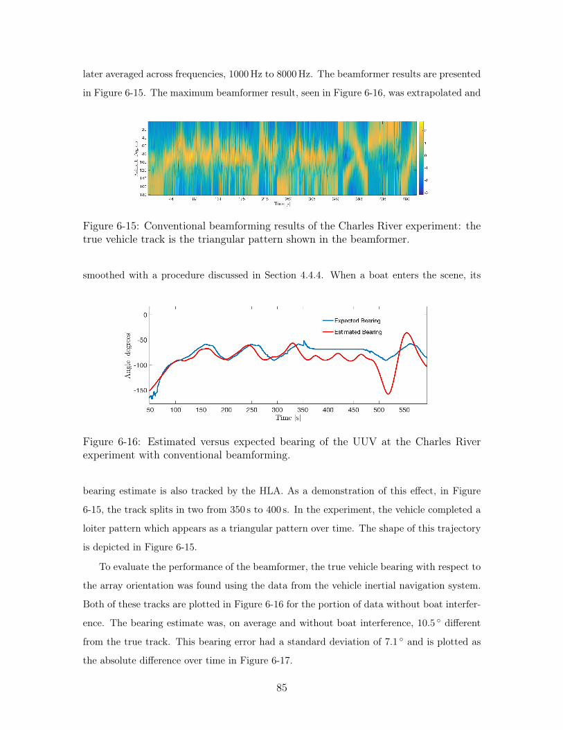
later averaged across frequencies, 1000Hz to 8000Hz. The beamformer results are presented

in Figure 6-15. The maximum beamformer result, seen in Figure 6-16, was extrapolated and

Figure 6-15: Conventional beamforming results of the Charles River experiment: thetrue vehicle track is the triangular pattern shown in the beamformer.

smoothed with a procedure discussed in Section 4.4.4. When a boat enters the scene, its

Figure 6-16: Estimated versus expected bearing of the UUV at the Charles Riverexperiment with conventional beamforming.

bearing estimate is also tracked by the HLA. As a demonstration of this effect, in Figure

6-15, the track splits in two from 350 s to 400 s. In the experiment, the vehicle completed a

loiter pattern which appears as a triangular pattern over time. The shape of this trajectory

is depicted in Figure 6-15.

To evaluate the performance of the beamformer, the true vehicle bearing with respect to

the array orientation was found using the data from the vehicle inertial navigation system.

Both of these tracks are plotted in Figure 6-16 for the portion of data without boat interfer-

ence. The bearing estimate was, on average and without boat interference, 10.5 ∘ different

from the true track. This bearing error had a standard deviation of 7.1 ∘ and is plotted as

the absolute difference over time in Figure 6-17.

85

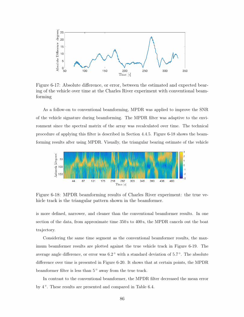
Figure 6-17: Absolute difference, or error, between the estimated and expected bear-ing of the vehicle over time at the Charles River experiment with conventional beam-forming

As a follow-on to conventional beamforming, MPDR was applied to improve the SNR

of the vehicle signature during beamforming. The MPDR filter was adaptive to the envi-

ronment since the spectral matrix of the array was recalculated over time. The technical

procedure of applying this filter is described in Section 4.4.5. Figure 6-18 shows the beam-

forming results after using MPDR. Visually, the triangular bearing estimate of the vehicle

Figure 6-18: MPDR beamforming results of Charles River experiment: the true ve-hicle track is the triangular pattern shown in the beamformer.

is more defined, narrower, and cleaner than the conventional beamformer results. In one

section of the data, from approximate time 350 s to 400 s, the MPDR cancels out the boat

trajectory.

Considering the same time segment as the conventional beamformer results, the max-

imum beamformer results are plotted against the true vehicle track in Figure 6-19. The

average angle difference, or error was 6.2 ∘ with a standard deviation of 5.7 ∘. The absolute

difference over time is presented in Figure 6-20. It shows that at certain points, the MPDR

beamformer filter is less than 5 ∘ away from the true track.

In contrast to the conventional beamformer, the MPDR filter decreased the mean error

by 4 ∘. These results are presented and compared in Table 6.4.

86

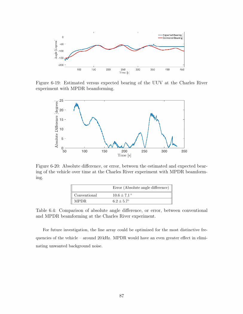
Figure 6-19: Estimated versus expected bearing of the UUV at the Charles Riverexperiment with MPDR beamforming.

Figure 6-20: Absolute difference, or error, between the estimated and expected bear-ing of the vehicle over time at the Charles River experiment with MPDR beamform-ing.

Error (Absolute angle difference)

Conventional 10.6± 7.1 ∘

MPDR 6.2± 5.7∘

Table 6.4: Comparison of absolute angle difference, or error, between conventionaland MPDR beamforming at the Charles River experiment.

For future investigation, the line array could be optimized for the most distinctive fre-

quencies of the vehicle – around 20 kHz. MPDR would have an even greater effect in elimi-

nating unwanted background noise.

87

88

Chapter 7

Conclusion

The role of UUVs has evolved from mapping and MCM to advanced missions of tracking

plumes [79] and under ice exploration [19]. Technology has enabled these complex missions,

specifically by advancing small-SWAP sensors to improve navigation, autonomy to make

decisions without a human operator in a highly dynamic, unpredictable environment, and

energy to go long distances without refueling.

However, improved UUV capabilities have led UUVs to play a role in asymmetric warfare.

Countries with less-established navies can even the playing field by leveraging UUVs: UUVs

are low-cost, easy to deploy, covert, difficult to detect, act as force-multipliers, and reduce

the risk to personnel because they are autonomous.

As a result, the U.S. Department of Defense has a prime interest in investing in counter-

UUV technology. For example, DARPA has published a BAA for "Open Ocean Counter

Unmanned Underwater Vehicle (OOCUUV) Study" [30], Strategic Systems Program for

Nuclear Weapons Security has called for small business innovation research (SBIR) for "Un-

manned Undersea Vehicle (UUV) Detection and Classification in Harbor Environments" [4],

and the U.S. Department of the Navy has requested a "Counter-Unmanned Undersea Vehi-

cle (C-UUV) Capability Demonstration for the Stiletto Maritime Demonstration Program"

[2].

This thesis is a response to this growing need – to create technology to covertly detect

and track UUVs with confidence and protect ships, harbors, and submarines from UUVs of

malicious intent. The solution discussed in this thesis could also be integrated into existing

passive acoustic surveillance systems.

89

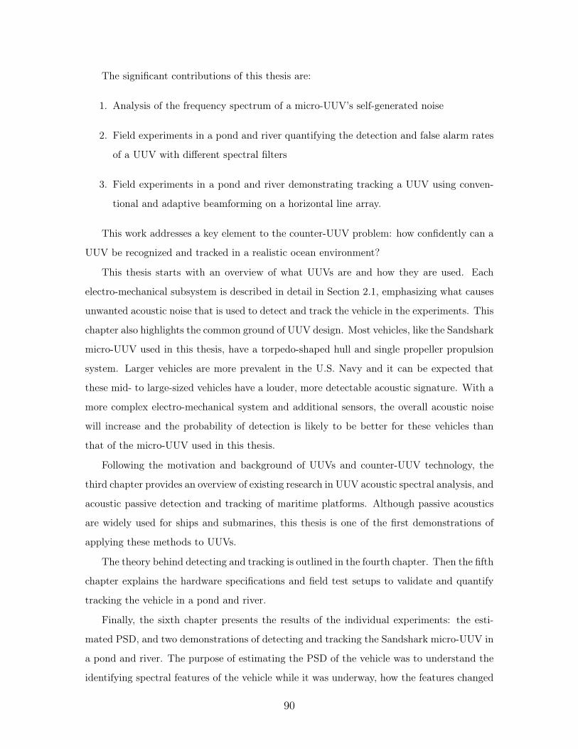
The significant contributions of this thesis are:

1. Analysis of the frequency spectrum of a micro-UUV’s self-generated noise

2. Field experiments in a pond and river quantifying the detection and false alarm rates

of a UUV with different spectral filters

3. Field experiments in a pond and river demonstrating tracking a UUV using conven-

tional and adaptive beamforming on a horizontal line array.

This work addresses a key element to the counter-UUV problem: how confidently can a

UUV be recognized and tracked in a realistic ocean environment?

This thesis starts with an overview of what UUVs are and how they are used. Each

electro-mechanical subsystem is described in detail in Section 2.1, emphasizing what causes

unwanted acoustic noise that is used to detect and track the vehicle in the experiments. This

chapter also highlights the common ground of UUV design. Most vehicles, like the Sandshark

micro-UUV used in this thesis, have a torpedo-shaped hull and single propeller propulsion

system. Larger vehicles are more prevalent in the U.S. Navy and it can be expected that

these mid- to large-sized vehicles have a louder, more detectable acoustic signature. With a

more complex electro-mechanical system and additional sensors, the overall acoustic noise

will increase and the probability of detection is likely to be better for these vehicles than

that of the micro-UUV used in this thesis.

Following the motivation and background of UUVs and counter-UUV technology, the

third chapter provides an overview of existing research in UUV acoustic spectral analysis, and

acoustic passive detection and tracking of maritime platforms. Although passive acoustics

are widely used for ships and submarines, this thesis is one of the first demonstrations of

applying these methods to UUVs.

The theory behind detecting and tracking is outlined in the fourth chapter. Then the fifth

chapter explains the hardware specifications and field test setups to validate and quantify

tracking the vehicle in a pond and river.

Finally, the sixth chapter presents the results of the individual experiments: the esti-

mated PSD, and two demonstrations of detecting and tracking the Sandshark micro-UUV in

a pond and river. The purpose of estimating the PSD of the vehicle was to understand the

identifying spectral features of the vehicle while it was underway, how the features changed

90

over time, and to derive the spectral filters for energy detection. This was accomplished by

measuring the acoustic noise from the vehicle in a pool environment. The vehicle revealed a

PSD that had a standard deviation of about 20 %. The fluctuation in the PSD, represented

as a standard deviation or error, is not surprising, given that the propeller acoustic energy

is broadband and random. The vehicle also exhibited strong, high-frequency tones between

16 kHz and 18 kHz, which were actually aliased from the true frequency of about 20 kHz.

With information from the PSD estimate, different spectral filters were applied to the

acoustic data collected in the pond and river experiments to increase the true detection rate

of the UUV. ROC curves were produced to find the optimal energy detection threshold.

The highest performing filter was the combination of the PSD filter (as a frequency shaping

filter) with the bandpass filter from 16 kHz to 18 kHz. For the two in-water experiments,

realistic inference occurred, like boats passing by.

For the Jenkins Pond experiment, the tracking and detection results yielded worse per-

formance than the Charles River experiment for two reasons. First, a broadband interferer

disrupted the beamforming results. Secondly, the strong tone of the vehicle of 20 kHz was

aliased down to 800Hz instead of 17.5 kHz, as in the Charles River experiment. In the lower

frequency range, there is more background noise. Despite these shortcomings, the bandpass

filter on 800Hz decreased the probability of false alarms from 49.5 % to 36.0 %. The beam-

former results were within 7.4 degrees of the true track for conventional beamforming and

5.2 degrees for MPDR.

The Charles River case, on the other hand, had the same sampling rate as the data

acquisition system used to derive the PSD estimate. Therefore, the PSD could be used as a

filter on the Charles River data, increasing the frequencies of importance. The other filter

applied to the Charles River dataset was a bandpass filter on the 16 kHz to 18 kHz range.

The combination of the two filters performed the best, resulting in a probability of detection

of 96.0% and probability of false alarms of 18.3% which, compared to no filter, decreased

false alarms by 18.8%. The beamformer output produced 10.6 degrees within the true track

of the vehicle and 6.2 degrees for the beamformer with MPDR.

In order to improve upon these results, additional analysis of the causes of the acoustic

PSD of the vehicle is recommended. The PSD estimate test should also be repeated with

acoustic sensors off-board the vehicle to remove the possibility of shielding. The detection

and tracking experiments could be repeated with higher sampling rates to prevent aliasing

91

the identifiable high frequency tones. In addition, more UUV types can be investigated –

particularly larger vehicles which are more commonly used – to confirm the hypothesis that

they have a similarly shaped PSD estimate but overall louder signature.

For future field tests, interferers like the broadband noise found in Jenkins Pond, and

more generally, boats passing by, should be analyzed to prevent false alarms and improve the

beamformer output. By understanding the environmental noise, predicting the confidence

level or ideal threshold can be found for more scenarios. As noted in the Section 4.3.4,

energy thresholding is highly dependent on the background noise levels.

Since the UUV showed strong high frequency tones while underway, the acoustic hori-

zontal line array (HLA) should be optimized with this in mind. The next iteration of the

HLA should be equipped spatially and temporally to track a 20 kHz signal that is emitted

by the vehicle.

To take the experiment a step further, one should consider different environments like

open ocean and multi-vehicle tracking experiments. Furthermore, tracking UUVs on-board

moving platforms such as submarines, ships, and other UUVs is of interest, particularly in

areas of the ocean where a bottom-mounted array isn’t feasible, available, or practical. On

the processing side, a predictive model using the dynamics of the UUV could be incorporated

into estimating the global track of the vehicle. An example of target motion analysis is

using a Kalman filter. Lastly, acoustic propagation models could be leveraged to test the

performance of the detection algorithm under different conditions. The PSD estimate of the

vehicle could be used as input to the model.

With the rapid improvement of technology in UUVs, the list of possible scenarios to

test and prepare for against UUVs of malicious intent is constantly being added to. The

core issue of the counter-UUV problem is unchanged, however: to confidently and covertly

detect and track UUVs to understand their intent. With two demonstrations in realistic

environments, this thesis shows that, indeed, despite the challenges of countering UUVs,

they can be found and tracked with identifiable spectral features. The findings of this thesis

contribute one step forward in security technology to protect against the potential threat of

UUVs to harbors, ships, and submarines.

92

Bibliography

[1] Bluefin Robotics. http://www.versusrisk.com/en/bluefin-robotics/.

[2] Counter-Unmanned Undersea Vehicle (C-UUV) Hosted by the Stiletto MaritimeDemonstration Program. Technical report, ASD Rapid Reaction Technology Office,Stiletto Maritime Demonstration Platform.

[3] Curve Fit: Smooth response data. https://www.mathworks.com/help/curvefit/smooth.html.

[4] Department of the Navy (DoN) 15.2 Small Business Innovation Research (SBIR) Pro-posal Submission Instructions. Technical report, Office of Naval Research (ONR).

[5] Design Considerations of MOOS-IvP. https://oceanai.mit.edu/ivpman/pmwiki/pmwiki.php?n=Helm.HelmDesignIntro.

[6] HTI-96-Min Hydrophone Series. http://www.hightechincusa.com/products/hydrophones/hti96min.html.

[7] HYbrid Coordinate Ocean Model (HYCOM). https://hycom.org/.

[8] One ROC Curve and Cutoff Analysis. Technical report, NCSS Statistical Software.

[9] Raspberry Pi 3 Model B- Specifications. https://www.raspberrypi.org/products/raspberry-pi-3-model-b/.

[10] REMUS and Mine Countermeasures. https://www.onr.navy.mil/en/About-ONR/History/tales-of-discovery/remus.

[11] Trapezoidal numerical integration. https://www.mathworks.com/help/matlab/ref/trapz.html.

[12] A Survey of Missions for Unmanned Undersea Vehicle. Technical report, RAND Cor-poration, Santa Monica, 2009.

[13] U.S. underwater drone seized by China, Pentagon says. https://www.cbsnews.com/news/china-seizes-us-underwater-drone-pentagon/, 2016.

[14] DS-USB-1608FS-Plus. Technical report, Measurement Computing, 2017.

[15] Promode R. Bandyopadhyay. Highly maneuverable biorobotic underwater vehicles. InSpringer Handbook of Ocean Engineering, pages 281–300. 2016.

[16] J. Bellingham. Autonomous Underwater Vehicles (AUVs). In Encyclopedia of OceanSciences, pages 212–216. 2001.

93

http://www.versusrisk.com/en/bluefin-robotics/

https://www.mathworks.com/help/curvefit/smooth.html

https://www.mathworks.com/help/curvefit/smooth.html

https://oceanai.mit.edu/ivpman/pmwiki/pmwiki.php?n=Helm.HelmDesignIntro

https://oceanai.mit.edu/ivpman/pmwiki/pmwiki.php?n=Helm.HelmDesignIntro

http://www.hightechincusa.com/products/hydrophones/hti96min.html

http://www.hightechincusa.com/products/hydrophones/hti96min.html

https://hycom.org/

https://www.raspberrypi.org/products/raspberry-pi-3-model-b/

https://www.raspberrypi.org/products/raspberry-pi-3-model-b/

https://www.onr.navy.mil/en/About-ONR/History/tales-of-discovery/remus

https://www.onr.navy.mil/en/About-ONR/History/tales-of-discovery/remus

https://www.mathworks.com/help/matlab/ref/trapz.html

https://www.mathworks.com/help/matlab/ref/trapz.html

https://www.cbsnews.com/news/china-seizes-us-underwater-drone-pentagon/

https://www.cbsnews.com/news/china-seizes-us-underwater-drone-pentagon/

[17] Brian Borowski, Alexander Sutin, Heui-Seol Roh, and Barry Bunin. Passive acous-tic threat detection in estuarine environments. International Society for Optics andPhotonics, 6945(Optics and Photonics in Global Homeland Security IV), 2008.

[18] A. M. Bradley, M. D. Feezor, H. Singh, and F. Yates Sorrell. Power systems forautonomous underwater vehicles. Oceanic Engineering, IEEE Journal of, 26(4):526–538, 2001.

[19] Andrew S. Brierley, Paul G. Fernandes, Mark A. Brandon, Frederick Armstrong,Nicholas W. Millard, Steven D. McPhail, Peter Stevenson, Miles Pebody, James Per-rett, Mark Squires, Douglas G. Bone, and Gwyn Griffiths. Antarctic Krill Under SeaIce: Elevated Abundance in a Narrow Band Just South of Ice Edge. Science Magazine,295(8 March):1890–1892, 2002.

[20] Kevin Brinkmann and Jörg Hurka. Broadband Passive Sonar Tracking. GI Jahresta-gung, pages 812–817, 2009.

[21] Mario P. Brito and Gwyn Griffiths. Autonomy: Risk assessment. In Springer Handbookof Ocean Engineering, pages 527–544. 2016.

[22] John S. Canning. A Definitive Work on Factors Impacting the Arming of UnmannedVehicles. Technical Report May, Naval Surface Warfare Center, Dahlgren, 2005.

[23] Chris Lo. Persistent littoral surveillance: automatedcoast guards. https://www.naval-technology.com/features/featurenavy-persistent-littoral-surveillance-auvs-uuvs/, 2012.

[24] Kil Woo Chung, Alexander Sutin, Alexander Sedunov, and Michael Bruno. DEMONacoustic ship signature measurements in an urban harbor. Advances in Acoustics andVibration, 2011(i), 2011.

[25] Bryan Clark. Game Changers – Undersea Warfare. Technical report, Center forStrategic and Budgetary Assessments, 2015.

[26] Michael Corinthios. Energy and Power Spectral Densities. In Signals, Systems, Trans-forms, and Digital Signal Processing with MATLAB, chapter 12, pages 825–863. CRCPress, 2009.

[27] Denise Crimmins and Justin Manley. What are auvs, and why do we usethem? https://oceanexplorer.noaa.gov/explorations/08auvfest/background/auvs/auvs.html, 2008.

[28] J. Cuschieri and F. Debiesme. Characterizing the Sources of Noise and Vibration ona Small Autonomous Submersible. International Congress and Exhibition on NoiseControl Engineering, (August):1–6, 2000.

[29] J.M. Cuschieri, M. Dhanak, and D. Vendittis. AUV Self Noise Control and AcousticSignature Meaurements. Technical report, Department of Ocean Engineering, FloridaAtlantic University, Boca Raton, 1998.

[30] DARPA. Special Notice DARPA-SN-16-11 1: Open Ocean Counter Unmanned Un-derwater Vehicle (OOCUUV) Study. Technical report, 2016.

94

https://www.naval-technology.com/features/featurenavy-persistent-littoral-surveillance-auvs-uuvs/

https://www.naval-technology.com/features/featurenavy-persistent-littoral-surveillance-auvs-uuvs/

https://oceanexplorer.noaa.gov/explorations/08auvfest/background/auvs/auvs.html

https://oceanexplorer.noaa.gov/explorations/08auvfest/background/auvs/auvs.html

[31] Ross L. Dawe. Detection Threshold Modelling Explained. pages 1–76, 1997.

[32] N. N. De Moura, J. M. De Seixas, and Ricardo Ramos. Passive Sonar Signal Detectionand Classification Based on Independent Component Analysis. Sonar Systems, pages93–103, 2011.

[33] Dan E. Dudgeon and Richard T. Lacoss. An Overview of Automatic Target Recogni-tion. The Lincoln Laboratory Journal, 6(1):3–10, 1993.

[34] J. Dzielski, M. DeLorme, A. Sedunov, P. Sammut, and M. Tsionskiy. Guidance ofan unmanned underwater vehicle using a passive acoustic threat detection system.Waterside Security Conference (WSS), 2010 International, pages 1–4, 2010.

[35] Megan Eckstein. Navy: Future Undersea Warfare Will Have Longer Reach, Op-erate With Network of Unmanned Vehicles. https://news.usni.org/2016/03/24/navy-future-undersea-warfare-will-have-longer-reach-operate-with/network-of-unmanned-vehicles, 2016.

[36] Megan Eckstein. DARPA, BAE Systems Developing Small Unmanned Under-water Vehicles to Hunt Enemy Submarines. https://news.usni.org/2017/07/18/darpa-bae-systems-developing-small-uuv-to-conduct-active-sonar/sub-hunting-on-behalf-of-us-navy-subs, 2017.

[37] Joshua Edwards and Dennis Gallagher. Mine and Undersea Warfare for the Future,2014.

[38] Frank Ehlers. Cooperative Vehicle Target Tracking. In Springer Handbook of OceanEngineering, pages 499–515. 2016.

[39] Donald Eickstedt and Michael Benjamin. Cooperative Target Tracking in a DistributedAutonomous Sensor Network. In OCEANS 2006, pages 1–6. IEEE, sep 2006.

[40] Donald P Eickstedt. Adaptive Sampling in Autonomous Marine Sensor Networks. PhDthesis, Massachusetts Institute of Technology, Woods Hole Oceanographic Institute,2006.

[41] Donald P. Eickstedt, Michael R. Benjamin, Henrik Schmidt, and John J. Leonard.Adaptive control of heterogeneous marine sensor platforms in an autonomous sensornetwork. IEEE International Conference on Intelligent Robots and Systems, pages5514–5521, 2006.

[42] Criag Fields, Ralph Semmel, and James Shields. DSB Task Force Report on Next-Generation Unmanned Undersea Systems. Technical report, Defense Science Board,Washington, DC, 2016.

[43] L. Fillinger, A.J. Hunter, M. Zampolli, and M.C. Clarijs. Passive acoustic detectionof closed-circuit underwater breathing apparatus in an operational port environment.The Journal of the Acoustical Society of America, 132(10):700671121–14800503, 2012.

[44] Laurent Fillinger, Pascal De Theije, Mario Zampolli, Alexander Sutin, Hady Salloum,Nikolay Sedunov, and Alexander Sedunov. Towards a passive acoustic underwater sys-tem for protecting harbours against intruders. 2010 International Waterside SecurityConference, WSS 2010, 2010.

95

https://news.usni.org/2016/03/24/navy-future-undersea-warfare-will-have-longer-reach-operate-with/network-of-unmanned-vehicles



https://news.usni.org/2017/07/18/darpa-bae-systems-developing-small-uuv-to-conduct-active-sonar/sub-hunting-on-behalf-of-us-navy-subs



[45] Sydney J. Freedberg. Underwater Bloodhounds: DARPA’s Robot Subs. https://breakingdefense.com/2017/07/underwater-bloodhounds-darpas-robot-subs/,2017.

[46] Lee Freitag, Matthew Grund, Chris Chris Von Alt, Roger Stokey, and Thomas Austin.A Shallow Water Acoustic Network for Mine Countermeasures Operations with Au-tonomous Underwater Vehicles. Underwater Defense Technology (UDT), pages 1–6,2005.

[47] David Fries and William Kirkwood. Non-acoustic sensors. In Springer Handbook ofOcean Engineering, pages 423–439. 2016.

[48] Franz-Stefan Gady. Confirmed: US Navy Launches Under-water Drone From Sub. https://thediplomat.com/2015/07/confirmed-us-navy-launches-underwater-drone-from-sub/, 2015.

[49] John Gebbie, Martin Siderius, and J. S. Allen. Passive Acoustic Array Harbor SecurityApplications. Marine Technology Society Journal, 45(3):103–110, 2011.

[50] John Gebbie, Martin Siderius, and John S. Allen III. Aspect-dependent radiated noiseanalysis of an underway autonomous underwater vehicle. Journal of Acoustical Societyof America, 2012.

[51] John Gebbie, Martin Siderius, Reid Mccargar, John S Allen III, and Grant Pusey.Localization of a noisy broadband surface target using time differences of multipatharrivals. Journal of Acoustical Society of America, 2013.

[52] John Gebbie, Martin Siderius, Peter L. Nielsen, and James Miller. Passive localizationof noise-producing targets using a compact volumetric array. Journal of AcousticalSociety of America, 2014.

[53] Gwyn Griffiths, Peter Enoch, and Nicholas W. Millard. On the radiated noise of theAutosub autonomous underwater vehicle. ICES Journal of Marine Science – ICESJournal of Marine Science, 58(58):1195–1200, 2001.

[54] Matthew Grund, Lee Freitag, James Preisig, and Keenan Ball. The PLUSNet under-water communications system: Acoustic telemetry for Undersea Surveillance. Oceans2006, 2006.

[55] Ricardo Gutierrez-Osuna. Introduction to Speech Processing. Technical report, Per-ception, Sensing, Instrumentation Lab, Texas A&M University.

[56] Per Espen Hagen, Oyvind Hegrenes, Bjorn Jalving, Oiyvind Midtgaard, Martin Wiig,and Ove Ken Hagen. Making AUVs truly autonomous. In OCEANS 2007, pages 1–4.IEEE, 2007.

[57] Michael J. Hamilton, Stephanie Kemna, and David Hughes. Antisubmarine warfareapplications for autonomous underwater vehicles: The GLINT09 sea trial results.Journal of Field Robotics, 27(6):890–902, nov 2010.

[58] Oistein Hasvold, Nils J. Storkersen, Sissel Forseth, and Torleif Lian. Power sources forautonomous underwater vehicles. Journal of Power Sources, 162(2 SPEC. ISS.):935–942, 2006.

96

https://breakingdefense.com/2017/07/underwater-bloodhounds-darpas-robot-subs/

https://breakingdefense.com/2017/07/underwater-bloodhounds-darpas-robot-subs/

https://thediplomat.com/2015/07/confirmed-us-navy-launches-underwater-drone-from-sub/

https://thediplomat.com/2015/07/confirmed-us-navy-launches-underwater-drone-from-sub/

[59] Jason D. Holmes, William M. Carey, and James F. Lynch. Results from the Nan-tucket Sound autonomous underwater vehicle towed hydrophone array experiment.The Journal of the Acoustical Society of America, 120, 2006.

[60] Jason D. Holmes, William M. Carey, and James F. Lynch. An overview of unmannedunderwater vehicle noise in the low to mid frequencies bands. Acoustical Society ofAmerica, 9, 2010.

[61] Paul Hornsby. Autonomous Underwater Vehicles Capability and Trends. Technicalreport, Royal Australian Navy, 2016.

[62] John Howard. Fixed SONAR Systems the History and Future of the UnderwaterSilent Sentinel. The Submarine Review, pages 1–12, 2011.

[63] Stephanie Kemna, Michael J. Hamilton, David T. Hughes, and Kevin D. LePage.Adaptive autonomous underwater vehicles for littoral surveillance. Intelligent ServiceRobotics, 4(4):245–258, 2011.

[64] James C. Kinsey, Ryan Eustice, and Louis L. Whitcomb. A Survey of Underwa-ter Vehicle Navigation: Recent Advances and New Challenges. IFAC Conference ofManoeuvring and Control of Marine Craft (MCMC 2006), 88:1–12, 2006.

[65] John J. Leonard and Alexander Bahr. Autonomous underwater vehicle navigation. InSpringer Handbook of Ocean Engineering, pages 341–357. 2016.

[66] Naomi Ehrich Leonard. Cooperative vehicle environmental monitoring. In SpringerHandbook of Ocean Engineering, pages 441–458. 2016.

[67] Pierre F.J. Lermusiaux, Tapovan Lolla, Patrick J. Haley, Konuralp Yigit, Mattheus P.Ueckermann, Thomas Sondergaard, and Wayne G. Leslie. Science of autonomy: Time-optimal path planning and adaptive sampling for swarms of ocean vehicles. In SpringerHandbook of Ocean Engineering, pages 481–497. 2016.

[68] Te-Chih Liu and Henrik Schmidt. AUV-Based Seabed Target Detection and Tracking.IEEE, 2002.

[69] T. Lolla, P.J. Haley, and P.F.J. Lermusiaux. Path planning in multi-scale ocean flows:Coordination and dynamic obstacles. Ocean Modelling, 94:46–66, 2015.

[70] Ray Mabus. Autonomous Undersea Vehicle Requirement for 2025. Technical report,U.S. Navy, Washington, DC, 2016.

[71] Darren K. Maczka, Davide Spinello, Daniel J. Stilwell, Aditya S. Gadre, and Wayne L.Neu. Coordinated tracking of an acoustic signal by a team of autonomous underwatervehicles. AUVSI Unmanned Systems North America Conference 2009, 2:1016–1033,2009.

[72] Robert C. Manke and Raymond J. Christian. Asymmetry in Maritime Access andUndersea Anti-Access/Area-Denial. Technical Report August, Office of the Directorof Undersea Warfare, 2007.

[73] Adam Mara. Bluefin Sandshark. Technical report, General Dynamics - BluefinRobotics, Quincy, 2018.

97

[74] Matthew Ritchey. Unmanned Undersea Vehicles: An Asymmetric Tool for Sea Denial.Master’s thesis, Naval War College, 2008.

[75] Alejandro Mendez, Teresa J. Leo, and Miguel A. Herreros. Current state of technologyof fuel cell power systems for autonomous underwater vehicles. Energies, 7(7):4676–4693, 2014.

[76] George L. Ogden, Lisa M. Zurk, Mark E. Jones, and Mary E. Peterson. Extractionof small boat harmonic signatures from passive sonar. The Journal of the AcousticalSociety of America, 129(107), 2011.

[77] Alan V. Oppenheim and George C. Verghese. Power Spectral Density. MIT Open-CourseWare: 6.011 Introduction to Communication, Control, and Signal Processing,pages 183–195, 2010.

[78] Alan V. Oppenheim, Alan S. Willsky, and S. Hamid Nawab. Signals and Systems.Prentice Hall, Upper Saddle River, 1997.

[79] Stephanie Petillo, Henrik Schmidt, and Arjuna Balasuriya. Constructing a DistributedAUV Network for Underwater Plume-Tracking Operations. International Journal ofDistributed Sensor Networks, 2012.

[80] Mark Pomerleau. DOD plans to invest $600M in unmanned under-water vehicles. https://defensesystems.com/articles/2016/02/04/dod-navy-uuv-investments.aspx, 2016.

[81] H. Rice, S. Kelmenson, and L. Mendelsohn. Geophysical navigation technologies andapplications. PLANS 2004. Position Location and Navigation Symposium (IEEE Cat.No.04CH37556), pages 618–624.

[82] M. Samseer. US Navy uses undersea wireless technology torecharge UUVs. https://www.naval-technology.com/uncategorised/newsus-navy-uses-undersea-wireless-technology-to-recharge-uuvs/4657347/, 2015.

[83] Henrik Schmidt, Michael R Benjamin, Stephanie M Petillo, and Raymond Lum.Nested autonomy for distributed ocean sensing. In Springer Handbook of Ocean En-gineering, pages 459–479. 2016.

[84] Science and Technology Organization Centre for Maritime Research and Experimen-tation Cooperative. Cooperative Antisubmarine Warfare. Technical report, CMRE,La Spezia.

[85] Mae L. Seto. Marine Robot Autonomy. Springer Science & Business Media, 2012.

[86] Martin Siderius and John Gebbie. Ocean Ambient Noise Studies for Improved SonarProcessing. Technical report, Electrical and Computer Engineering, Portland StateUniversity, 2012.

[87] Erik Sofge. MIT Submarine Is Most Autonomous Robot Ocean Researcher Yet. https://www.popularmechanics.com/technology/robots/a12502/4285189/, 2009.

98

https://defensesystems.com/articles/2016/02/04/dod-navy-uuv-investments.aspx

https://defensesystems.com/articles/2016/02/04/dod-navy-uuv-investments.aspx

https://www.naval-technology.com/uncategorised/newsus-navy-uses-undersea-wireless-technology-to-recharge-uuvs/4657347/



https://www.popularmechanics.com/technology/robots/a12502/4285189/

https://www.popularmechanics.com/technology/robots/a12502/4285189/

[88] Milica Stojanovic and Pierre-Philippe J. Beaujean. Acoustic Communication. SpringerHandbook of Ocean Engineering, pages 359–386, 2016.

[89] Milica Stojanovic and James Preisig. Underwater acoustic communication chan-nels: Propagation models and statistical characterization. Communications Magazine,IEEE, 47(1):84–89, 2009.

[90] Dan Suchman and Thomas Meurling. Integrated underwater intruder detection sys-tem. In 2010 International WaterSide Security Conference, pages 1–8. IEEE, 2010.

[91] Shelby Sullivan. Mobile Offboard Command, Controland Attack (MOCCA). https://www.darpa.mil/program/mobile-offboard-clandestine-communications-and-approach.

[92] Harry L Van Trees. Characterization of Space-time Processes. In Optimum ArrayProcessing: Part IV of Detection, Estimation, and Modulation Theory, chapter 5.John Wiley & Sons, Inc., 2002.

[93] Harry L. Van Trees. Optimum Waveform Estimation. In Optimum Array Processing:Part IV of Detection, Estimation, and Modulation Theory, chapter 6. John Wiley &Sons, Inc., 2002.

[94] Harry Van Trees. Arrays and Spatial Filters. In Optimum Array Processing: Part IVof Detection, Estimation, and Modulation Theory, chapter 2, pages 17–89. John Wiley& Sons, Inc., 2002.

[95] Michael S. Triantafyllou and Franz S. Hover. Maneuvering and Control of MarineVehicles. Massachusetts Institute of Technology, pages 105–110, 2003.

[96] Edward Tucholski. Detection Theory. In Underwater Acoustics and Sonar SP411Handouts and Notes, chapter 15. Annapolis, 2006.

[97] U.S. Navy. The Navy Unmanned Undersea Vehicle (UUV) Master Plan. 2004.

[98] Rebecca Willet. Receiver Operating Characteristic ( ROC ) Curve. In ECE 830,chapter 8, pages 1–21. University of Wisconsin-Madison, Madison, 2014.

[99] Russell B. Wynn, Veerle A.I. Huvenne, Timothy P. Le Bas, Bramley J. Murton, Dou-glas P. Connelly, Brian J. Bett, Henry A. Ruhl, Kirsty J. Morris, Jeffrey Peakall,Daniel R. Parsons, Esther J. Sumner, Stephen E. Darby, Robert M. Dorrell, andJames E. Hunt. Autonomous Underwater Vehicles (AUVs): Their past, present and fu-ture contributions to the advancement of marine geoscience. Marine Geology, 352:451–468, 2014.

[100] Xuri Yu, Tommy Dickey, James Bellingham, Derek Manov, and Knut Streitlien. Theapplication of autonomous underwater vehicles for interdisciplinary measurements inMassachusetts and Cape Cod Bays. Continental Shelf Research, 22:2225–2245, 2002.

[101] Z. Y. Zhang. Diver Detection Sonars and Target Strength: Review and Discussions.14th International Congress on Sound & Vibration, pages 1–8, 2007.

[102] Richard Zimmerman, Gerald L. D’Spain, and C. David Chadwell. Decreasing theradiated acoustic and vibration noise of a mid-size AUV. IEEE Journal of OceanicEngineering, 30(1):179–187, 2005.

99

https://www.darpa.mil/program/mobile-offboard-clandestine-communications-and-approach

https://www.darpa.mil/program/mobile-offboard-clandestine-communications-and-approach

Demonstration of Passive Acoustic Detection and Tracking of ...

Documents