Demographic Window to Aging in the Wild: Constructing Life ...

Demographic Window, H. G. Muller et al. 1

Demographic Window to Aging in the Wild: Constructing Life

Tables and Estimating Survival Functions from Marked Individuals

of Unknown Age

Hans-Georg Muller1, Jane-Ling Wang1, James R. Carey2,3, Edward P. Caswell-Chen4, Carl Chen4,

Nikos Papadopoulos2 and Fang Yao5

1Department of Statistics, University of California, Davis, One Shields Ave., Davis, CA 95616, USA

2Department of Entomology, University of California, Davis, One Shields Ave., Davis, CA 95616, USA

3Center for the Economics and Demography of Aging, University of California, Berkeley, CA 94720,

USA

4Department of Nematology, University of California, Davis, One Shields Ave., Davis, CA 95616, USA

5Department of Statistics, Colorado State University, Fort Collins, CO 82523, USA

March 17, 2004

Correspondence

James R. Carey, Department of Entomology, University of California, Davis, One Shields Ave., Davis,

CA 95616, USA. Tel: +1 530 752 6217; fax: +1 530 752 1537; e-mail: [email protected]


Summary

We address the problem of establishing a survival schedule for wild populations. A demographic

key identity is established that leads to a method whereby age-specific survival and mortality can be

deduced from a marked cohort life table that is established for individuals that are randomly sampled

at unknown age and marked, with subsequent recording of time-to-death. This identity permits to

construct life tables from data where the birthdate of subjects is unknown. An analogous key identity

is established for the continuous case where the survival schedule of the wild population is related to

the density of the survival distribution in the marked cohort. These identities are explored for both

life tables and continuous lifetime data. For the continuous case, they are implemented with statistical

methods using nonparametric density estimation methods to obtain flexible estimates for the unknown

survival distribution of the wild population. The analytical model provided here serves as a starting

point to develop more complex models for residual demography, i.e., models for estimating survival of

wild populations where age-at-entry is unknown and using remaining information in randomly encoun-

tered individuals. This is a first step towards step a broad new concept of ’expressed demographic

information content of marked or captured individuals’.

Keywords: capture, demographic identity, density estimation, information content, life table, nonpara-

metric estimation, remaining lifetime, residual demography, survival function.


Introduction

The life table is one of the most important tools in demographic and gerontological research because

it is used to characterize the mortality and survival properties of cohorts and to quantify the actuarial

rate of aging. The historical application of classical life table methods in aging science has been largely

restricted to the use of mortality data from either humans or experimental animals maintained in

the laboratory or to life tables based on capture-recapture methods to assess aging in wild populations

(Udevitz & Ballachey, 1998). In both applications, it is mandatory that age-at-entry is known. This has

limited the use of life tables since in the analysis of field populations one often encounters and marks

individuals of unknown age. However, capture-recapture and other current field methods generally

require capturing and marking of young individuals, or alternatively of individuals of known age, for

monitoring throughout their lives until they die.

The predominance of capture-recapture methods has had a limiting effect on the use of flexible

nonparametric statistical methods that make minimal assumptions on survival schemes, and have the

desirable property that they do not presume statistical parametric survival models. Since in nonpara-

metric modeling one does not specify the functional form of hazard or survival functions, these methods

require the exact recording of lifetimes and therefore are not applicable to usual capture-recapture

designs which correspond to usually coarsely graded life tables (Lebreton et al. 1992, Williams 2002).

Because of the importance of the life table in aging research and the growing interest in understanding

aging in the wild (Austad 1993, Congdon et al. 1994, Finch 2001, Reznick et al. 2001, Tatar & Yin 2001),

the case of life table analysis with unknown age at entry and the analogous situation for continuous

lifetimes is clearly of high interest. We describe a life table identity that, by making certain key

assumptions, enables us to estimate the age-specific life table rates from data based on the mark, release,

and monitoring of randomly-captured individuals of unknown age from the time of their entry into the


study (i.e. marking) to their death. We also discuss an identity for the continuous case where marked

animals are continuously monitored until their death. Continuous monitoring, when feasible, enables

the continuous version of the analysis which provides us with substantially more detailed information

about the behavior of survival functions and hazard rates (force of mortality). Our approach can also

be used in conjunction with life tables that are obtained from capture-recapture experiments in those

situations where age-at-entry is unknown. Current designs of capture-recapture experiments however

are not amenable to continuous lifetime analysis with the preferred flexible nonparametric methods,

allowing for the construction of hazard rate estimates.

Consider a population that is assumed to be stable, stationary and closed. Individuals are captured

with equal probability at an unknown age and marked, then their time-to-death is recorded. The

question we address is this: Can the information on time-to-death for this randomly-captured marked

subgroup provide the necessary information to construct a life table for the population at large? We

will demonstrate that the answer to this question is affirmative because of a life table identity that

reveals a mathematical relationship between the distribution of deaths in the marked cohort and the

age structure of the original population. Individuals in the captured and marked sample are assumed

to have remaining lifetimes as in the wild. We note that this model may be particularly adequate for

some human populations.

The problem of constructing a survival schedule from incomplete data has been studied in anthro-

pology (Muller et al. 2002) and has applications to human populations such as the !Kung and the Ache

for which only incomplete demographic data are available (Hawkes et al. 1998; Howell 1979; Hill &

Hurtado 1996; Jones et al. 2002). An anthropologist may encounter a group of people whose ages are

unknown but whose remaining lifetime can be recorded. The key identity, on which the reconstruction

of the survival schedule that we propose is based, asserts that for such situations a life table for the


population can be obtained, under certain assumptions. Application of the key identity then establishes

a new way to construct life tables and estimate survival functions.

We derive this key identity for both discrete life tables and situations which are modeled by continu-

ous survival times. In the continuous case, this identity is a consequence of a close relationship between

the density of the remaining lifetimes in a cohort of randomly sampled subjects and the survival sched-

ule of the population from which the subjects were sampled. We provide statistical implementations of

this identity by applying suitably adapted nonparametric density estimation methods. The proposed

model is developed for a stable, stationary and closed population but possesses sufficient flexibility to

allow for modifications of these assumptions.

The concept and techniques that we describe in this paper will help to advance understanding of

senescence in the wild in all three areas that were outlined by Gaillard and co-workers (Gaillard et

al. 1994). First, refinements of this concepts have the potential to improve the reliability of survival

data because, unlike the approach used in virtually all long-term field studies in which only newborn

are marked and their survival monitored throughout their lives, this approach estimates survival using

information from individuals first marked at any age. Therefore for many species it may be possible to

mark many more individuals than are available from only a single (newborn) age group and therefore

increase sample size. Second, this approach introduces new biological concepts for measuring senescence

in the wild that differ from Nesse’ (1988) intensity of selection, Finch’s (1990) mortality rate doubling

time, Promislow’s (1991) log slope mortality, and Abrams’ (1993) fitness cost of senescence. Our method

is moreover a useful addition to capture-recapture studies with unknown age-at-entry.

The method we outline in this paper focuses on the information content of wild-caught, living in-

dividuals and will ultimately not only include information on survival that can be used to estimate

actuarial aging as in conventional approaches, but information on fertility, behavior, mating and other


life history categories that can be used to shed new light on senescence in the wild. Third, the meth-

ods we introduce here will provide new techniques for expanding the taxonomic horizons of senescence

studies in the wild beyond mammals to include other vertebrates such as birds, reptiles, fishes and

amphibians as well as invertebrates ranging from nematodes to insects. The method will be especially

important for studying aging of invertebrates in the wild such as nematodes that cannot be marked and

released into the wild for later recapture.

A Key Demographic Identity

The data on remaining lifetime after capture and marking that are obtained from the marked sample

are assembled in a “marked sample life table”. Assuming that the process of capture and marking does

not alter an individual’s remaining lifespan, the corresponding “marked sample” and “wild” life tables

are compared for a hypothetical situation in Table 1.

That it is possible to obtain the survival schedule in the wild, as summarized by the wild life table,

from the marked sample life table is due to a basic relationship between these two life tables. Assuming

that the population is stable, stationary and closed, i.e., is neither increasing nor decreasing, and without

immigration or emigration, the number of subjects of age x is cx = lx/∑

ly = c0lx (Caswell, 2001, see

Table 1 for definitions). The death rates in the marked sample life table at age x′ are by definition

d∗x′ = l∗x′ − l∗x′+1. These death rates are generated by subjects that enter the marked sample life table at

various (unknown) ages, survive to “marked age” (i.e., age counted in days after capture and marking)

x′ and do not survive to “marked age” x′ + 1. For all subjects that enter the marked sample cohort at

age z, the contribution to d∗x′ is therefore

czlz+1

lz

lz+2

lz+1. . .

lz+x′

lz+x′−1(1− lz+x′+1

lz+x′) = cz(

lz+x′

lz− lz+x′+1

lz) = c0(lz+x′ − lz+x′+1),


where lz refers to the survival function or survival schedule of the wild population at age z.

The contributions of subjects entering the marked sample life table at various ages are additive.

Therefore, adding the contributions over all ages of entry z,

d∗x′ =∑

z

c0(lz+x′ − lz+x′+1) = c(0)lx′ = cx′ ,

and this relationship implies that the columns cx indicating the age distribution in the wild life table

and d∗x indicating the distribution of deaths in the marked sample life table are identical. We can see

from Table 1 that this is indeed the case for the hypothetical case considered there. As lx = cxc0

, this

relationship between the two life tables leads to

lx =d∗xd∗0

,

thus enabling the reconstruction of the survival schedule lx in the wild life table from the survival

schedule l∗x of the marked sample life table.

Statistical estimates implementing this probabilistic relationship can be easily found, for example by

plugging in empirical observed frequencies for l∗x and d∗x, thus replacing expected population values as

they appear in Table 1 with their corresponding sample estimates. Based on the binomial distribution

of these observed frequencies, we can derive large-sample confidence intervals for the resulting estimates

of lx. Details and formulas are provided in the Appendix.

Continuous Lifetimes

These considerations can be extended to the case where age-at-death is considered to be measured

on a continuous scale and the smooth nature of the underlying survival distributions can be discerned.

The power of analyzing hazard functions from continuous lifetimes has been illustrated in Muller &


Wang (1984). Information loss and recovery of features related to smoothness and derivatives such as

hazard rates from aggregated survival data as encountered in life tables is well known (Muller et al.

1997, Wang et al. 1998). For these reasons, it is therefore clearly preferable to work with continuous

lifetime data rather than life tables whenever feasible. Therein lies one of the promises of the proposed

methodology – the continuous case is supported without the need to specify a parametric model for the

survival distribution as is usually required. The downside of parametric modeling is lack of flexibility

since these models are tied to the correctness of the assumed parametric model, and such an assumption

cannot be easily verified. The continuous model can be implemented whenever the marked cohorts can

be continuously monitored.

In the following, we discuss the continuous version of the key identity. This identity enables us

to estimate hazard rates and other continuous features of survival distributions by means of flexible

nonparametric curve estimation methods. Denoting by X the age-at-death (lifetime) for an individual

in the wild, by F (x) = P (X > x) the survival function in the wild, where x is a continuous age

variable and P denotes probability, we find for the density of the age-distribution in the wild c(x) =

F (x)/∫∞0 F (x) dx, and consequently F (x) = c(x)

c(0) .

The unknown age A at the time of capture and marking and the unknown age-at-death X are

related with the known remaining lifetime X∗ of an individual by X∗ = X − A. Denote the densities

of the distributions of X,X∗ by fX , fX∗ , and consider the conditional density fX(·|X ≥ x) of lifetime

conditional on the event that the individual survives to age x. Then one obtains for the density fX∗(a)

of X∗, evaluated at the age-at-death a,

fX∗(a) =∫ ∞

0c(x)fX(x + a|X ≥ x) dx =

∫ ∞

0

F (x)∫F (a)da

fX(x + a)F (x)

dx

=F (a)∫F (a)da

= c(a).


This relationship implies the key identity for the continuous case,

F (x) =fX∗(x)fX∗(0)

,

providing the relationship between the marked cohort mortality and survival in the wild. This type of

relationship has been noted previously in the literature on renewal processes (Doob, 1948; Feller, 1968;

Winter, 1989). Statistical estimation and inference based on this continuous version of the key identity

is discussed in the next section.

Estimating the Survival Schedule of the Wild Population

Given a sample of continuous lifetimes X∗1 , . . . , X∗

n that are observed in the marked sample cohort and

measured in terms of relative age counted from the time of marking, we may substitute nonparametric

kernel density estimators (compare for example Muller 1997) for fX∗(z), given by

fX∗(z) =1

nh

n∑

i=1

K

(x−X∗

i

h

).

Here h = h(n) is a sequence of bandwidths and K is a kernel function. Specific kernel functions are

listed in the Appendix.

We note that we implement a flexible nonparametric smoothing approach that does not depend on a

model assumption for the survival schedule as likelihood based and also Bayesian methods would require

when dealing with continuous lifetimes. Given the enormous plasticity of mortality schedules in biolog-

ical populations, these methods are very limited in their applicability while nonparametric methods do

not make any assumptions on the underlying survival distributions except for some basic smoothness.

In return, a bandwidth or smoothing parameter h in the above kernel density estimator needs to be

specified to control the trade-off between variance and bias of the resulting nonparametric estimates.


Methods for data-adaptive specification of bandwidths and also efficient numerical implementations of

the above estimator are described in Muller (1997).

We then obtain asymptotically consistent estimates of the survival function of the wild population,

ˆF (x) =fX∗(x)

fX∗(0).

The implementation of this estimate is less straightforward than it may seem. One difficulty is that

the estimates fX∗(0) that appear in the denominator are density estimates at a boundary point of the

support of the data and therefore are subject to higher variability than density estimates in the interior

of the support (Muller & Wang 1994). We replace the kernel K in the definition of the kernel density

estimator above by a boundary kernel K0 when estimating the density of X∗ at the boundary point

x = 0 (see end of Appendix). A second difficulty is that the above estimate is not necessarily a survival

function, which by definition is monotone declining from 1 to 0. This can be ensured by adding a

monotonization step through the pool adjacent violators algorithm (PAVA; Robinson & Dykstra, 1988).

We note that using analogous kernel density estimators f ′X∗(x) for the derivative of fX∗ , we may

obtain estimates for the density f of the survival schedule of the wild cohort, f(x) = −f ′X∗(x)/fX∗(0).

Analogously, estimates for the hazard rate h(x) = f(x)/F (x) are obtained as h(x) = −f ′X∗(x)/fX∗(x).

To obtain the density derivative estimates that appear in these formulas we replace the kernel K in the

kernel density estimator above by a derivative kernel K1 (often chosen as K1 = K(1), see Appendix)

and the scaling factor 1/(nh) by 1/(nh2). The construction of confidence intervals and thus inference

for these nonparametric estimates can be obtained through asymptotic methods. The asymptotic argu-

ments, corresponding variance estimates and resulting formulas for confidence intervals are summarized

in the Appendix.

To assess the age at capture for a subject for which an additional lifetime x was observed in the


marked cohort life table, we may use the conditional density fA|X∗(a|x) = fX(x + a)/F (x) to infer the

conditional expectation

E(A|X∗ = x) =1

F (x)

∫ ∞

x(z − x)fX(z) dz.

Plugging the above estimates into the right hand side of this equation then leads to consistent estimates

of conditional mean age at capture. We note that monotonized density estimates similar to those above

were proposed by Watelet & Winter (1991) in a reliability setting.

Illustration

We illustrate the reconstruction of the survival schedule of the wild population from the observations

made on the marked sample in a simulation study. The underlying survival schedule of the wild popu-

lation is modeled as the survival function of a real cohort. The starting point is a cohort consisting of

1000 female Mediterranean fruit flies, Ceratitis capitata, commonly known as the medfly, whose survival

has been described and analyzed in Carey et al. (1998).

Using acceptance-rejection sampling based on the graph of the survival function for these 1000 flies,

we randomly sample N flies (with replacement) to create one simulated marked sample. Each of the

flies that is selected for the marked sample has a random age, following the age distribution of the flies

in the entire “wild population”, and also an associated remaining lifetime that is recorded as “marked

lifespan”. Kernel density estimation as described above is implemented by local linear smoothing after

an initial prebinning step (see Muller, 1997) and combined with the PAVA method.

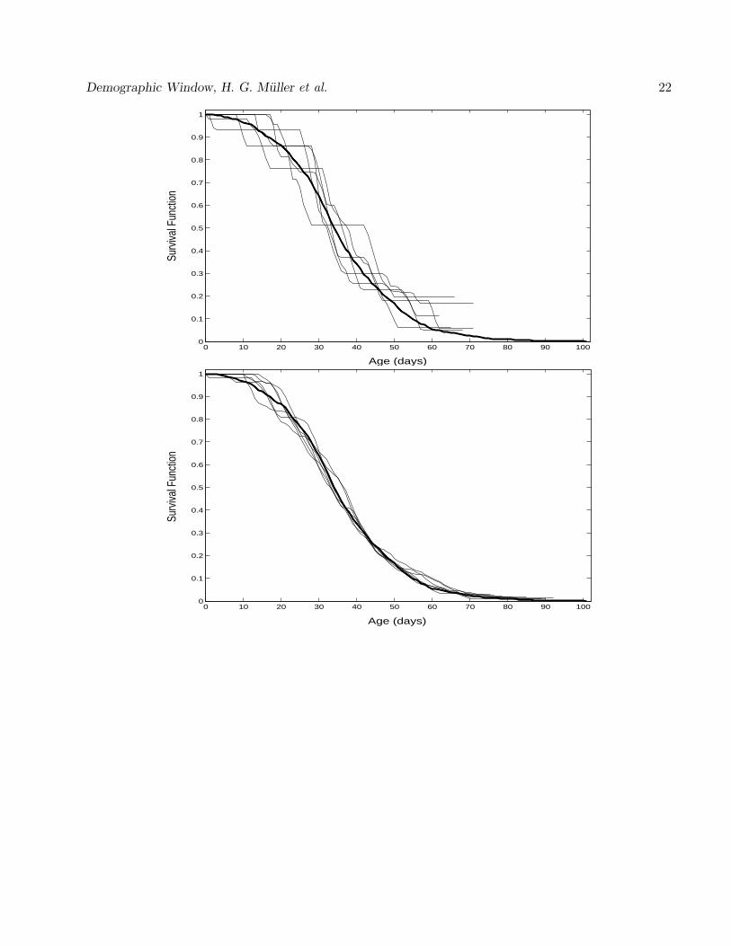
The resulting survival function estimates along with the target survival function for six generated

marked sample cohorts of sizes N = 1000 and N = 50 can be seen in Figure 1. We find that the method

of reconstructing the survival schedule of the wild population works very well for the larger sample and


reasonably well for the smaller sample. The infant survival estimates show a higher degree of variability

than the survival estimates for the mid-age period since not very many early deaths will be recorded in

the marked cohort.

Discussion: Window on Aging in the Wild and a Generalization

In this paper we demonstrated that age-specific life tables can be constructed from mortality data

derived from randomly-captured individuals of unknown age in stable, stationary and closed populations.

The importance of our model is that it provides a starting point to develop more complex models whose

purpose is to estimate the life table properties of populations based on more realistic assumptions (non-

stable, non-stationary populations). However, we believe that the significance of the general approach

extends beyond the life table and applies to the concept of expressed information content of marked (or

captured) individuals. For the current case the expressed information is the remaining post-capture life

span of marked individuals that is used to estimate the life table of the population at large.

The idea of expressed information content generalizes if it is assumed that: (1) the experiences

of individuals early in life influence the expression and pattern of their life history traits (mortality,

reproduction, behavior) later in life; and (2) these patterns expressed in later life can be traced to

early-life experience. The concept of extracting knowledge of both an individual’s age and its early-life

experience to gain insights into the demographic and gerontological characteristics of the field population

then can be used as the conceptual foundation for a new sampling concept for understanding aging in

the wild. Examples of the types of information that can be extracted from wild-caught (or marked)

individuals at the individual level include remaining life span, age-specific reproduction (relative to time

of capture), details of reproduction including birth interval, clutch size, post-reproductive period, overall

patterns of individual reproduction, total reproduction, and time from capture to first egg, timing and


magnitude of peak reproduction (Carey et al. 1998, Muller et al. 2001), mating status and frequency of

mating, behavioral measures such as calling (males, see Papadopoulos et al. 2002), mating, oviposition,

and overall activity, and physiological measures such as metabolic rate.

We believe that this new concept for extracting information about aging in the wild is important

for several reasons. First, life course analysis will both encourage and require a deep understanding of

the interdependencies of various components of an individual’s life course including reproduction, be-

havior, and death. In particular the approach will require an understanding of the relationship between

reproduction at young ages and mortality risk at older ages, the age patterns of reproduction that are

unique to different stages in the adult life course, and the linkages between different behavioral patterns

and death. Second, the approach will encourage a greater integration of laboratory and field studies.

Specifically, the method will require the creation of reference ’libraries’ consisting of the life history

patterns of individuals maintained under different conditions in the laboratory. These ’libraries’ will be

used for comparing the observed life history patterns (birth and death) of wild-caught flies maintained

in the laboratory. Third, the results of studies using the methods we propose to develop will shed new

light on both aging and aging structure of wild populations. This includes aging data on populations of

invertebrate species such as C. elegans which are difficult to study under natural conditions in the wild

but which are extraordinarily important model organisms in aging science (Gershon & Gershon, 2002;

Reznick, 1993). The combination of laboratory and field studies will provide the means for testing vari-

ous theories about aging in the wild and also for testing models used in both forecasting and back-casting.

Appendix: Asymptotic Confidence Intervals and Variances

Based on the estimation of the survival schedule of the wild population, one can derive asymptotic

confidence intervals for important characteristics of the survival schedule of the wild population. This


includes confidence intervals and associated inference for the survival function F (x) for discrete and

continuous lifetimes, and the density fX∗(x) and hazard rate hX∗(x) for continuous lifetimes. Another

option is to employ a suitable bootstrap.

We first investigate confidence intervals for the survival function F (x) for discrete lifetimes, i.e., the

survival schedule at age x, given by lx = d∗x/d∗0, where x is an arbitrary nonnegative integer. Let d0 and

d∗x denote the estimates obtained by plugging in empirical observed frequencies for d∗0 and d∗x. Let Wn(x)

denote the number of deaths in (x, x + 1]. It is easily seen that Wn(x) ∼ B(n, d∗x), for x = 0, 1, . . ., and

d∗x/d∗0 = Wn(x)/Wn(0), where B(n, d∗x) denotes the binomial distribution with n trials and probability

of success d∗x, and n is the total number of subjects. Then from the Central Limit Theorem, one can

obtain the asymptotic joint distribution of the multinomial random variable (Wn(x),Wn(0))T which

is N2((d∗x, d∗0)T , Σ), where N2 denotes the bivariate normal distribution, and Σ is a 2× 2 matrix with

(Σ)11 = d∗x(1− d∗x), (Σ)22 = d∗0(1− d∗0), and (Σ)12 = (Σ)21 = −d∗xd∗0. Applying the delta method leads

to the asymptotic normal distribution of ˆF (x),

(lx − lx)/√

nD−→ N(0,

d∗x(1− d∗x)d∗0

2 +d∗x

2(1− d∗0)d∗0

3 − 2d∗x2

d∗02 ),

Then the 100(1−α)% confidence interval of lx is obtained by substituting the empirical estimates of lx

and applying Slutsky’s Theorem,

lx ± Φ(1− α/2)√

d∗x(1− d∗x)/d∗20 + d∗2x (1− d∗0)/d∗30 − 2d∗2x /d∗20

where Φ(·) is the the cumulative distribution function of the standard normal random variable.

For the case of continuous lifetimes, the survival function is estimated by ˆF (x) = fX∗(x)/fX∗(0).

Assume that a kernel K supported on [−1, 1] is used for fX∗(x) and the boundary kernel K0 supported

on [−1, 0] for fX∗(0). The bandwidth h for the kernel density estimates fX∗(x) and fX∗(0) is assumed to

satisfy h → 0 and nh →∞, as n →∞. For any fixed x, when n is sufficiently large, one has h < x− h,


i.e., no X∗i ’s are included in both [0, h] and [x− h, x + h], whence the estimates fX∗(x) and fX∗(0) are

asymptotically independent. From standard results for kernel density estimation (see Muller 1997 for

references), one can easily obtain the asymptotic joint distribution of [fX∗(x), fX∗(0)] as follows,

√nh{fX∗(x)−E[fX∗(x)], fX∗(0)− E[fX∗(0)]} D−→ N2(0,

fX∗(x)‖K‖2, 0

0, fX∗(0)‖K0‖2

),

which is bivariate normal with mean vector 0. Here ‖K‖2 =∫

K2(u)du and ‖K0‖2 =∫

K20 (u)du.

Since the bias E[fX∗(x)] − fX∗(x) = O(h2) for both x = 0 and x > 0, we can ignore biases for small

values of h. Assuming this is the case and applying the delta method, we obtain the asymptotic normal

approximation to the distribution of ˆF (x) = fX∗(x)/fX∗(0),

ˆF (x)− F (x) ≈ N(0,1

nh[fX∗(x)‖K‖2

f2X∗(0)

+f2

X∗(x)(‖K0‖2

f3X∗(0)

]).

Then the 100(1 − α)% confidence interval for F (x) is obtained by substituting the consistent kernel

estimates fX∗(x) and fX∗(0) for fX∗(x) and fX∗(0) in the formula, applying Slutsky’s theorem, i.e., the

100(1− α)% confidence interval for F (x) is

ˆF (x)± Φ(1− α/2)√

[fX∗(x)‖K‖2/f2X∗(0) + f2

X∗(x)‖K0‖2/f3X∗(0)]/(nh).

To construct the confidence interval for the density estimate f(x) = f ′X∗(x)/fX∗(0), we note that the

derivative estimate f ′X∗(x) has slower convergence rate than fX∗(0). Slutsky’s theorem implies that

f ′X∗(x)/fX∗(0) is asymptotically equivalent to f ′X∗(x)/fX∗(0). From the asymptotic distribution of

the kernel estimator for the derivative f ′X∗(x), and ignoring the bias terms as argued earlier, one has

f ′X∗(x)−f ′X∗(x) ≈ N(0, fX∗(x)‖K1‖2/(nh3)), where K1 is the kernel function used in f ′X∗(x). Thus the

asymptotic distribution of the density estimate f ′(x) is approximately N(0, fX∗(x)‖K1‖2/[nh3f2X∗(0)]),

and the 100(1−α)% confidence intervals can be obtained by substituting the kernel estimates for f ′X∗(x)

and fX∗(0), whence one obtains the intervals

f ′(x)± Φ(1− α/2)√

fX∗(x)‖K1‖2/[nh3f2X∗(0)].


Similarly, the 100(1−α)% confidence interval for the hazard rate h(x), estimated by h(x) = f ′X∗(x)/fX∗(x),

is obtained by

h(x)± Φ(1− α/2)√

fX∗(x)‖K1‖2/[nh3f2X∗(x)].

We note that common choices for kernels for interior, boundary and derivative estimation K, K0, K1

are K(x) = 0.75(1 − x2) on [−1, 1], K0(x) = 12(x + 1)(x + 1/2) on [−1, 0], and K1(x) = −(3/2)x on

[−1, 1].

Acknowledgments

This research was supported by NIH grant P01-AG08761 and NSF grant DMS-02-04869. We thank

J. Cardenas for technical assistance, L. Harshman, L. Partridge, and A. Yashin for discussion and J.

Vaupel and K. Wachter for comments on a previous draft.

References

Abrams PA (1993) Does Increased Mortality Favor the Evolution of More Rapid Senescence? Evolution

47, 877-887.

Austad SN (1993) Retarded senescence in an insular population of Virginia opossums (Didelphis vir-

giniana). Journal of Zoology 229, 695-708.

Carey JR (2002) Development of a model for assessing the demography of a captive cohort. Unpub-

lished manuscript.

Carey JR, Liedo P, Muller HG, Wang JL, Chiou JM (1998) Relationship of age patterns of fecundity to

mortality, longevity, and lifetime reproduction in a large cohort of Mediterranean fruit fly females.

Journal of Gerontology – Biol. Sci. 53, 245-251.


Caswell H (2001) Matrix population models: construction, analysis, and interpretation (2nd ed). Sun-

derland, Mass.: Sinauer Associates.

Congdon JD, Dunham AE, VanLobenSels RC (1994) Demographics of common snapping turtles

(Chelydra serpentina): Implications for conservation and management of long-lived organisms.

American Zoologist 34, 397-408.

Doob JL (1948) Renewal theory from the point of view of the theory of probability. Transactions of

the American Mathematical Society 63, 429.

Feller W (1968) Introduction to Probability Theory, vol. I. New York: Wiley.

Finch CE (1990) Longevity, Senescence, and the Genome. Chicago: The University of Chicago Press.

Finch CE (2001) History and prospects: symposium on organisms with slow aging. Experimental

Gerontology 36, 593-597.

Gaillard JM, Allaine D, Pontier D, Yoccoz NG, Promislow DEL (1994) Senescence in natural popula-

tions of mammals: A reanalysis. Evolution 48, 509-516.

Gershon H, Gershon D (2002) Caenorhabditis elegans–a paradigm for aging research: advantages and

limitations. Mechanisms in Ageing and Development 123, 261-274.

Hawkes K, O’Connell JF, Jones NGB, Alvarez H, Charnov EL (1998) Grandmothering, menopause,

and the evolution of human life histories. Proceedings of the National Academy of Sciences of the

United States of America 95, 1336-1339.

Hill K, Hurtado AM (1996) Ache Life History. New York: A. de Gruyter.

Howell N (1979) Demography of the Dobe !Kung. New York: Academic Press.


Jones NGB, Hawkes K, O’Connell JF (2002) Antiquity of postreproductive life: Are there modern

impacts on hunter-gatherer postreproductive life spans? American Journal of Human Biology 14,

184-205.

Lebreton, JD, Burnham, KP, Clobert, J, Anderson, DR (1992) Modelling survival and testing biological

hypotheses using marked animals: A unified approach with case studies. Ecological Monographs

62, 67-118.

Muller HG (1997) Density estimation. In Encyclopedia of Statistical Science (Kotz S, Read CB, Banks

DL, ed). New York: Wiley, pp. 185-200.

Muller HG, Carey JR, Wu D, Liedo P, Vaupel JW (2001) Reproductive potential predicts longevity

of female Mediterranean fruit flies. Proceedings of the Royal Society B 268, 445-450.

Muller HG, Love B, Hoppa R (2002) A semiparametric method for estimating paleodemographic

profiles from age indicator data. American Journal of Physical Anthropology 116, 1-14.

Muller HG, Wang JL (1994) Hazard rate estimation under random censoring with varying kernels and

bandwidths. Biometrics 50, 61-76.

Muller HG, Wang JL, Capra WB (1997). From lifetables to hazard rates: The transformation approach.

Biometrika 84, 881-892.

Papadopoulos NT, Carey JR, Katsoyannos BI, Kouloussis NA, Muller HG, Liu X (2002) Supine be-

haviour predicts time to death in Mediterranean fruit flies (Ceratitis capitata). Proceedings of

the Royal Society B 269, 1633-1637.

Papadopoulos NT, Katsoyannos BI, Kouloussis NA, Carey JR, Mller HG, Zhang Y. (2004) High sexual

calling rates predict extended life span in male Mediterranean fruit flies. Oecologia 138, 127-134.


Promislow DEL (1991) Senescence in natural populations of mammals: a comparative study. Evolution

45, 1869-1887.

Reznick D (1993) New model systems for studying the evolutionary biology of aging: crustacea. Ge-

netica 91, 79-88.

Reznick D, Buckwalter G, Groff J, Elder D (2001) The evolution of senescence in natural populations

of guppies (Poecilia reticulata): a comparative approach. Experimental Gerontology 36, 791-812.

Robertson T, Wright FT, Dykstra RL (1988) Order Restricted Statistical Inference. Wiley New York

Tatar M, Yin CM (2001) Slow aging during insect reproductive diapause: why butterflies, grasshoppers

and flies are like worms. Experimental Gerontology 36, 723-738.

Udevitz MS, Ballachey BE (1998) Estimating Survival Rates with Age-Structure Data. Journal of

Wildlife Management 62, 779-792.

Wang JL, Muller HG, Capra WB (1998). Analysis of oldest-old mortality: Lifetables revisited. Annals

of Statistics 26, 126-163.

Watelet L, Winter BB (1991) Nonparametric estimation of nonincreasing densities and use of data

from renewal processes. Communications in Statistics – Theory and Methods 20, 2073-2094.

Williams BK, Nichols JD, Conroy MJ (2002) Analysis and Management of Animal Populations. Aca-

demic Press, London.

Winter BB (1989) Joint simulation and forward recurrence times in a renewal process. Journal of

Applied Probability 26, 404-407.


Table 1: Illustration of the relationship between hypothetical ’wild’ and ’marked sample’ life tables

in the stationary case (from Carey, 2002). The ’wild’ cohort consists of Nx individuals at each age

x with corresponding schedules of survival lx and age structure cx = lx/∑

ly, with life table in the

leftmost subtable. The ’marked sample’ cohort consists of initially 20 ’marked’ individuals with the

same age structure as the ’wild’ cohort, all simultaneously entering the marked sample cohort at the

age of capture and marking x∗ = 0. Remaining lifetimes are recorded for the marked sample, Nx∗ is

the number of animals that remain alive at age x∗ after marking, and lx∗ is the survival schedule of

the marked sample cohort, with death rates dx∗ = lx∗+1 − lx∗ , as listed in the rightmost subtable. The

survival schedules separately for age cohorts x = 0, x = 1, x = 2 and x = 3 in dependency on marked

sample cohort age x∗ are listed in the corresponding columns of the sub-table in the middle. In this

hypothetical example, the initial marked sample cohort at marked sample cohort age x∗ = 0 has an age

structure identical to cx (bolded row in middle subtable is identical to bolded cx column of leftmost

sub-table). The key identity is revealed by the equality of bolded columns cx and dx∗ in leftmost and

rightmost sub-tables. This key relationship allows to deduce the wild survival schedule from the marked

sample survival schedule.

Wild Cohort Age Distribution in Marked

Sample Cohort

Marked Sample

x Nx lx cx x = 0 x = 1 x = 2 x = 3 x∗ Nx∗ lx∗ dx∗

0 40 1.000 0.40 0.40 0.30 0.25 0.05 0 20 1.00 0.40

1 30 0.750 0.30 0.30 0.25 0.05 1 12 0.60 0.30

2 25 0.625 0.25 0.25 0.05 2 6 0.30 0.25

3 5 0.125 0.05 0.05 3 1 0.05 0.05

4 0 0.000 0.00 0.00 4 0 0.00 0.00

100 2.5 1.95 1.00


Legend

Figure 1: Reconstruction of survival function of wild population from six simulated marked sample

cohorts of sizes N=50 (upper panel) and N=1000 (lower panel). This reconstruction is based on a key

demographic identity and corresponding nonparametric estimation methods as described in text. The

solid curve is the target survival function that corresponds to the observed survival schedule of a cohort

of medflies.


0 10 20 30 40 50 60 70 80 90 1000

0.1

0.2

0.3

0.4

0.5

0.6

0.7

0.8

0.9

1

Age (days)

Surv

ival F

unct

ion

0 10 20 30 40 50 60 70 80 90 1000

0.1

0.2

0.3

0.4

0.5

0.6

0.7

0.8

0.9

1

Age (days)

Surv

ival F

unct

ion

Demographic Window to Aging in the Wild: Constructing Life ...

Documents