Demand Side Management (DSM)

Demand Side Management (DSM) For

Efficient Use of Energy in the Residential Sector in Kuwait:

Analysis of Options and Priorities

Azeez Nawaf Al-enezi, BSc, MSc.

Submitted in partial fulfilment of the requirements for the degree of

Doctor of Philosophy

Institute of Energy and Sustainable Development, De Montfort University, Leicester

October 2010

ABSTRACT

The State of Kuwait has one of the largest per capita consumption in the world,

reaching 13061kWh in 2006 (Kuwait MEW, 2007). The power sector in Kuwait is not

commercially viable, due to the current under-pricing policy and heavily subsidized

tariff.

Kuwait needs to take action to meet the increased energy demand. A particular

challenge is peak summer demand when extreme heat increases air conditioning loads.

Peak demand reached 8900 MW in 2006, with a growth fast at an average rate 5.6%

during the last decade. The generated energy reached 47605 GWh in 2006 and is

growing fast at an average rate of 6.5%. Electricity demand is characterized by high

seasonal variations and low load factor.

The main objective of this research is to assess and evaluate the most effective

and robust Demand Side Management (DSM) measures that could achieve substantial

reductions in peak demand and electricity consumption in the residential sector.

The residential sector in Kuwait consumes about 65% of total electricity

consumption, and is characterized with inefficient use of energy due to several factors,

including very cheap energy price and lack of awareness.

To achieve the research objective, an integrated approach was used, including the

following steps:

• Performing a demand forecast and a building stock forecast across 10 years

period (2010 -2019) for the residential sector. The main types of dwellings in

Kuwait (villas, apartments and traditional houses) were considered in the

forecast.

• Conducting detailed energy audits and measurements on selected typical models

of residential dwellings. The aim of this process is to examine energy patterns

and identify the potential energy efficiency DSM measures.

• Performing a simulation process, to evaluate energy performance of the audited

dwellings and to estimate the potential DSM savings. Two basic scenarios were

2

considered in simulation, the first represents the base-case with actual existing

condition and the second for different DSM options.

• Analysis of identified technological DSM options (five) and recommended

policy DSM options (two) and ranking them in priority order using the Analytic

Hierarchy Process (AHP).

• Estimate the potential energy savings and peak demand reductions by the

implementation of identified DSM options. A building block approach is used to

estimate the aggregate impacts of DSM options and its reflection on the country

Load Duration Curve (LDC).

The research showed that a DSM portfolio consisting of the seven identified

measures, and through a dedicated programme, could have substantial reductions in

energy consumption and peak demand.

The research showed that the total accumulated energy savings across the

forecast period was estimated at approximately 37229 GWh, and the total peak demand

reductions during at the end of forecast (2019) reaches 1530 MW representing 8.9% Of

the overall peak load.

With respect to the type of dwelling, the research also indicated that the total net

revenues for the utility were estimated at: $292 million for villas, $79 million for

apartments and $47 million for traditional houses.

One of the important indicators showed as a result of implementing the

identified DSM measures is the positive environmental impact that could be achieved

by reducing CO2 total emissions by approximately 26.8 million tonne, which could

achieve an annual income of about $38.9 million.

Integrated DSM policy recommendations were formulated, including gradual

tariff adjustment, and more involvement by the utility, or government, in the creation of

sustainable DSM programmes.

3

CONTENTS PageABSTRACT 2 CONTENTS 4 LIST OF FIGURES 6 LIST OF TABLES 7 ABREVIATIONS ACKNOWLEDGEMENTS

10 11

Chapter 1: Introduction, Research Motivation and Organization of Work

12

1.1 Introduction 12 1.2 Research Motivation 13 1.3 Research Objective 14 1.4 Basic and Specific Research Questions 14 1.5 Research Methodology 15 1.6 Summary 16 Chapter 2: DSM Background and Techniques 17 2.1 The Concept of DSM 17 2.2 Standard DSM Load Shape Objectives 18 2.3 Conceptual Basis of DSM Research 20 2.4 World Experience in DSM and Lessons Learned 2.4.1 Experience of USA 2.4.2 Experience of European Union 2.4.3 Experience of United Kingdom 2.4.4 Experience of Thailand 2.4.5 Experience of Egypt 2.4.6 Lessons Learned

21 21 24 25 26 29 33

2.5 DSM Activities in Kuwait- Literature Review 2.6 Summary

34 35

Chapter 3 Demand Analysis and Forecast 37 3.1 Overview of Electricity Demand in Kuwait 3.2 Residential Sector in Kuwait 3.3 Energy Consumption by End-use Equipment 3.4 Baseline Scenario and Demand Forecast 3.5 Summary

37 41 44 45 46

Chapter 4: Energy Audits and Measurements 48 4.1 Introduction 48 4.2 Results of Energy Audits 48 4.3 Results of Measurements 52 4.4 Summary 58

4

Chapter 5: Building Simulation 60 5.1 Introduction 60 5.2 Simulation Tool Used 61 5.3 Simulation Scenarios and DSM Measures 64 5.4 Simulation Findings 67 5.5 Summary 74 Chapter 6: Analysis of Potential DSM Options

75

6.1 Introduction 75 6.2 Analysis of Audit and Simulation Results 6.2.1 Base Case Condition 6.2.2 DSM Energy Conservation Opportunities

75 75 76

6.3 Portfolio of DSM Technology Options 81 6.4 Selection of DSM Policy Options 6.4.1 Increase of Electricity Tariff 6.4.2 Energy Efficiency Labels and Standards

81 81 83

6.5 Summary 84 Chapter 7: Evaluation and Ranking of DSM Options 86 7.1 Introduction 86 7.2 Criteria for Evaluation and Ranking 7.2.1 The Analytic Hierarchy Process (AHP)

86 87

7.3 Features of Identified DSM Options 7.3.1 Impact of Tariff Increase 7.3.2 Energy Efficiency Standards and Labelling

88 90 90

7.4 Example of AHP Calculations 7.4.1 Expert Choice 7.4.2 Sensitivity Analysis

95 95 102

7.5 Summary 105 Chapter 8: Potential Impacts of Priority DSM Options 106

8.1 Introduction 106 8.2 Methodology 107 8.3 Baseline Demand Forecast 8.3.1 Demand Forecast for Residential Sector 8.3.2 Housing Forecast

109 112 113

8.4 Penetration Rate of DSM Options 8.4.1 Market Transformation

115 115

8.5 Unit Impact 124 8.6 Cumulative DSM Impacts 124

8.7 Summary 129 Chapter 9: Economical and Environmental Impacts

130

9.1 Introduction 130 9.2 Economic Benefits/Cost Analysis 9.2.1 Avoided Cost

130 131

5

9.2.2 Cost of Saved Energy (CSE) 9.2.3 Cost of Saved Capacity (CSC) 9.2.4 Cost of DSM Programme 9.2.5 Cost Effectiveness of DSM Programme 9.2.6 Economic Assumptions

132 133 133 140 142

9.3 Economic Results 142 9.4 Environmental Impacts 145 9.5 Summary 149

Chapter 10: Conclusions and Recommendations 151 10.1 Conclusions 151 10.2 Barriers To DSM Implementation 153 10.3 Funding and Incentives 156 10.4 Recommendations 10.4.1 Efficient Lighting Initiative 10.4.2 Green Building Initiative

156 158 159

10.5 Future Research Work 160 REFERENCES 163 APPENDICES 167

LIST OF FIGURES

Page Chapter 2 DSM Background and Techniques Figure 2.1 Standard DSM Load – Shape Objectives 18 Figure 2.4 Phased Approach to DSM In Egypt 32 Chapter 3 Residential Sector in Kuwait Figure 3.1 Development of Installed Capacity, Peak Load and Load Factor

(1995-2006) 38

Figure 3.2 Maximum and Minimum Demand During 2006 38 Figure 3.3 The Peak Load Profile on July 26, 2006 39 Figure 3.4 Monthly Load Factor for 2005 and 2006 40 Figure 3.5 The Development of Generated and Exported Energy 40 Figure 3.6 The Distribution of Final Energy Consumption by Sector 41 Figure 3.7 Electricity Consumption by Type of End-Use 45 Figure 3.8 Baseline Demand Forecast 46 Chapter 4 Energy Audits and Measurements Figure 4.1 (a) Monthly Consumption 2007 (Villa) 49 Figure 4.1 (b) Monthly Consumption 2007 (Apartment) 49 Figure 4.1 (c) Monthly Consumption 2007 (Traditional House) 50 Figure 4.2 Three Phase 4-Wire Connection Diagram 53 Figure 4.3 A Typical Single Line Diagram of Electrical System (Villa) 53 Figure 4.4 An Image of A Typical Villa in Kuwait 54 Figure 4.5 (a) Summer Daily Power Profile for a Villa (July 2008) 55 Figure 4.5 (b) Daily Power Profile for a Villa (January 2008) 56 Figure 4.6 (a) Summer Daily Power Profile for an Apartment (July 2008) 56

6

Figure 4.6 (b) Winter Daily Power Profile for an Apartment (Jan. 2008) 57 Figure 4.7 (a) Summer Daily Power Profile for a Traditional House (July 2008) 57 Figure 4.7 (b) Summer Daily Power Profile for a Traditional House (Jan. 2008) 58 Chapter 5 Building Simulation Figure 5.1 Major Components of Building Energy Analysis Simulation 63 Chapter 6 Analysis of Potential DSM Options Figure 6.1 Aggregate Annual Saving of DSM Options 79 Figure 6.2 Aggregate Impact of DSM Options on Peak Demand 79 Figure 6.3 Distribution of Total Consumption by End-Use 80 Figure 6.4 Portfolio of Proposed DSM Options 84 Chapter 7 Evaluation and Ranking of DSM Options Figure 7.1 AHP Block Diagram 93 Figure 7.2 Hierarchy Structure of DSM Options 98 Figure 7.4 (a) Performance Sensitivity Analysis Base Case with Saved Energy

Score “5” DSM 2 103

Figure 7.4 (b) Performance Sensitivity Analysis Saved Energy for DSM 2 is Higher by 40% than Base Case

104

Chapter 8 Potential Impacts of Priority DSM Options Figure 8.1 Steps of DSM Impacts Evaluation 107 Figure 8.2 The Peak Load Profile “26 July, 2006” 112 Figure 8.3 Baseline Forecast for Electricity Consumption (Total Final and

Residential) 113

Figure 8.4 Logistic S-Curve DSM Market Adoption 123 Figure 8.5 DSM Impacts on Final Energy Consumption (GWh) 127 Figure 8.6 DSM Impacts on Peak Demand 127 Figure 8.7 The Impact of DSM Options on Load Duration Curve 128 Chapter 9 Economical and Environmental Impacts Figure 9.1 Power Plants Consumption by Fuel Type 148

LIST OF TABLES

Page Chapter 1 Introduction, Research Motivation and Organization of

Work

Table 1.1 Development of Installed Capacity and Maximum Demand 13 Chapter 2: DSM Background and Techniques Table 2.1 Energy and Peak Demand Savings of Selected Programmes in

USA 24

Table 2.2 DSM Programme Savings in Thailand Through June 2000 29

Chapter 3 Potential DSM in The Residential Sector in Kuwait

7

Table 3.1 Projected Rate of Growth of The Kuwaiti Population 42 Table 3.2 Development of Households (1985-2005) 42 Table 3.3 Types and Numbers of Dwellings 43 Table 3.4 Electricity Consumption of Residential Consumers 44 Chapter 4 Energy Audits and Measurements Table 4.1 Typical Example of Audit Results 51 Table 4.2 (a) Summary of Measured Parameters (For Villas) 54 Table 4.2 (b) Summary of Measured Parameters (For Apartments) 54 Table 4.2 (c) Summary of Measured Parameters (For Traditional Houses) 55 Chapter 5 Building Simulation Table 5.1 (a) Input Data for Building Simulation for The Base Case 66 Table 5.1 (b) Input Data for Building Simulation With DSM Options 67 Table 5.2 Estimates of Monthly and Annual Energy Consumption (Base

Case) 68

Table 5.3 (a) Villa Monthly Simulation Results 71 Table 5.3 (b) Apartment Monthly Simulation Results 72 Table 5.3 (c) Traditional House Monthly Simulation Results 73 Chapter 6 Analysis of Potential DSM Options Table 6.1 DSM Impact on Annual Energy Consumption 78 Table 6.2 Impact of DSM Options on Peak Demand (July) 78 Table 6.3 Proposed Electricity Tariffs for Residential Consumers 82 Chapter 7 Evaluation and Ranking of DSM Options Table 7.1 Hierarchy Evaluation Criteria of DSM Options 89 Table 7.2 Features of Proposed Scores of Identified DSM Options 94 Table 7.3 (a) Pair Wise Comparison for "Saved Energy" 98 Table 7.3 (b) Pair Wise Comparison for "Saved Energy" (With Column

Totals) 99

Table 7.3 (c) Synthesized Matrix for “Saved Energy” 99 Table 7.4 Pair Wise Comparison for "Peak Load Reduction" 99 Table 7.5 Pair Wise Comparison for "Investment Cost" 100 Table 7.6 Pair Wise Comparison for "Payback Period" 100 Table 7.7 Pair Wise Comparison for "Penetration Rate" 100 Table 7.8 Pair Wise Comparison for "Technology Acceptance" 101 Table 7.9 Pair Wise Comparison Matrix for the Six Criteria (With Column

Totals) 101

Table 7.10 Priority Matrix for DSM Options (1) 102 Table 7.11 Priority Matrix for DSM Options (2) 104 Chapter 8 Potential Impacts of Priority DSM Options Table 8.1 Development of Energy and Power Demands from 2005 to 2010 111 Table 8.2 Development of Generated Energy and Peak Load (1995-2006) 111 Table 8.3 Electricity Consumption by Sector 113 Table 8.4 The Development of Private Buildings Stock 115 Table 8.5 Proposed New Electricity Tariff 119 Table 8.6 Proposed New Electricity Tariff for Residential Consumers 120

8

Table 8.7 Savings Potential of Tariff Increase (KISR Study) 121 Table 8.8 Assumptions for The Potential Impact of Tariff Increase on

Energy and Load 123

Table 8.9 (a) DSM Impacts by Type of Dwelling-Annual Energy Savings (GWh) (Scenario 1: Tariff Price Elasticity -0.04)

125

Table 8.9 (b) DSM Impacts by Type of Dwelling-Annual Energy Savings (GWh) (Scenario 2: Tariff Price Elasticity -0.10)

125

Table 8.10 (a) DSM Impacts by Type of Dwelling-Peak Demand Reductions (MW) – Scenario 1: Tariff Elasticity -0.04

126

Table 8.10 (b) DSM Impacts by Type of Dwelling-Peak Demand Reductions (MW) – Scenario 2: Tariff Elasticity -0.10

126

Table 8.11 DSM Energy Saving Impacts by DSM Option 128 Chapter 9 Economical and Environmental Impacts Table 9.1 Lighting System Basic Data 137 Table 9.2 Example of DSM Programme Cost for CFL Rebate Programme 139 Table 9.3 Residential Equipment Life Span 142 Table 9.4 Summary of Economic Impact Estimates by DSM Option (2010-

2019) 144

Table 9.5 Power Plants Energy Consumption in Billion Btu Classified by Fuel Type (2006)

147

Table 9.6 CO2 Emissions from Fuels Used in Kuwait Power Plants 148 Table 9.7 Annual Reductions of CO2 Emissions 148 Table 9.8 Economic Parameters of DSM Options (2010-2019) (Dollars in

$1000, Present Value) 149

9

ABREVIATIONS

AC Air Conditioner(s) AHP Analytic Hierarchy Process CER Certified Emission Reduction CFL Compact Fluorescent Lamp CO2 Carbon Dioxide COP Coefficient Of Performance DBET Department of Buildings and Energy Technologies DOE Department Of Energy (United States) DSM Demand Side Management ECC Energy Conservation Code ECO Energy Conservation Opportunity EER Energy Efficiency Ratio EIA Energy Information Administration ESCO Energy Service Company EVM Eigenvector Method GB Green Building GDP Gross Domestic Products GEF Global Environmental Facility GHG Greenhouse Gas GWh Gegawatt hour HVAC Heating, Ventilation and Air Conditioning IEA International Energy Agency KD Kuwaiti Dinar KISR Kuwait Institute for Scientific Research kW Kilowatt kWh Kilowatt hour LDC Load Duration Curve MEW Ministry Of Energy (Electricity and Water) M toe Million Ton Oil Equivalent MW Megawatt (1000 kW) OECD Organization for Economic Co-operation and Development

Countries SEER Seasonal Energy Efficiency Ratio TOE Ton Oil Equivalent TPES Total Primary Energy Supply UNDP United Nations Development Programme WB World Bank

10

ACKNOWLEDGEMENTS

I am truly very grateful to Dr Andrew Wright and Dr Ibrahim Abdalla for the

sincere help and the support during their supervision at my PhD study.

Considerable thanks go to Dr Greig Mill and Dr Simon Taylor for the

assessment of my previous work at the annual review meetings.

Moreover, I express my gratitude for Dr Ali Alhmoud and Dr Ahmad Almulla in

Kuwait Institute for Scientific Research for their advices and guidance.

Obviously I am grateful to Dr William Batty and Dr Simon Rees for their

examination of my thesis.

Needless to say, I thank my colleagues and staff at IESD and the members in the

Graduate School Office.

I am indebted to my family and relatives for their patience, love and

encouragement.

11

CHAPTER 1

INTRODUCTION, RESEARCH MOTIVATION AND

ORGANIZATION OF WORK

1.1 INRODUCTION

Utility demand-side management (DSM) is a way of managing the

demand for power by encouraging the customers to modify their level or pattern of

electricity usage. DSM was applied with some success in the developed countries and

especially in the USA. At least 92 technologies were listed in the literature1,2,3 ,that were

used in the USA for providing strategic conservation, peak clipping, peak shifting,

valley filling, flexible demand and strategic growth on the utility load shape.

In recent years, DSM has emerged as an efficient utility planning strategy for

reducing capacity shortages and improving system load factors4, although some

controversy exists about the magnitude and precise cost-effectiveness of DSM

implementation5.

Nowadays, DSM is considered as an essential part of the Integrated Resource

Planning (IRP) options to minimize social costs from the utility operation in meeting

the future demand.

In Kuwait the problem of power shortage, and even programmed power cut, has

been recently remarked due to the growing demand and the great waste of electrical

energy. Potential energy efficiency improvements and on-peak reduction were highly

recognize in several local studies and researches6,7,8,9,10, however, no DSM programmes

have been yet promoted.

The Ministry of Electricity and Water (MEW), is the only utility responsible for

generation, transmission and distribution of electricity in Kuwait. It has to meet the

growing demand for electricity by building new power plants that require high

investments. MEW is vertically integrated and has five power plants use heavy oil and

natural gas. The total installed capacity of MEW thermal power plants has reached

10313 MW in 2006, consisting of 9054 MW total capacity of steam turbine units and

1259 MW total capacity of gas turbine units11.

12

The following table shows the development of installed capacity, maximum

demand, Energy exported (sent out) to the grid and the load factor.

Table 1.1 Developments of Installed Capacity and Maximum Demand

Year 1996 1998 2000 2002 2004 2006 Avg.

Growth Rate

Installed Capacity (MW)

6898 7389 9189 9189 9689 10313 3.75%

Maximum Demand (MW)

5200 5800 6450 7250 7750 8900 5.1%

Exported Energy (TWh)

21.7 25.8 27.5 31.1 35.6 47.6 7.15%

Load Factor (%) 55.8 59.1 57.1 57.2 60.6 61.1 0.9%

Source: The Ministry of Electricity and Water, Electrical Energy Statistical Year Book, 2007 TWh = 1012 Wh

The present research work focuses on the potential DSM measures for the

residential sector and the evaluation of their impacts on the on-peak demand and

energy consumption from 2010 to 2019 (inclusive).

1.2 Research Motivation

The key motivating issues for this research work are: • From Table 1.1, it is clear, that the peak demand in Kuwait increased from 5200

MW in 1996 to 8900 MW in 2006, with an average growth rate about 5.1%. In

contrast, the average growth rate of maximum demand in most of the industrial

countries does not exceed 2-3%.

Based on MEW Statistical Year Book, the maximum load share per capita reached

2796 watts in 2006. Thus, MEW is facing great challenges; first to satisfy the

requirements of large investments for building new power plants, and second to take

the necessary actions for rational use of energy and decrease the rate of electricity

demand.

• Energy efficiency indicators provided by IEA show that Kuwait has, relatively,

much higher energy intensity. The energy intensity is expressed as the energy

content per GDP; for Kuwait the energy intensity for 2004 was 0.58 toe/GDP

13

Thousand $2000, while the world average is 0.29 and the OECD average is 0.19

toe/GDP Thousand $200012.

• The net electricity generation in Kuwait reached 13061 kWh per capita in 2006. By

international comparison, this level is extremely high. According to IEA statistics,

the world average of electricity consumption per capita is only 2516 kWh. This

means that Kuwait's per capita electricity consumption is about 5 times the world

average13.

• In Kuwait, the power sector is not commercially viable, due to the current under-

pricing policy and heavily subsidized tariff. MEW charges a flat tariff rate 2 fils (≈

US¢ 0.60)/kWh to almost all consumers, except for the owners of beach cabins

(chalets), they have to pay more (10 fils/ kWh). For all consumers no demand

charges are paid. Under these circumstances of cheap electricity prices the

consumers in Kuwait do not use electricity in an efficient way.

• Since the residential sector in Kuwait is the major consumer of electricity and it is

responsible for about 65% of total electricity consumption (estimated at 21 TWh in

2003), it is expected to have a good potential for DSM.

1.3 Research Objective

The core objective of this work is to assess and evaluate the most effective and

robust DSM measures that could achieve substantial reductions in peak demand and

electricity consumption in the residential sector. 1.4 Basic and Specific Research Questions

The basic research question could be formulated as follows:

What are the demand side management techniques, including technology measures and

policies which could be implemented in the residential sector and lead to a substantial

reduction in peak demand and energy consumption?

Consequently, the following specific questions have to be answered:

a) What will be the future energy use in the absence of any DSM activities?

b) How can demand side management resources offset the need for new power

plants in Kuwait?

14

c) What are the potential DSM priority options that could be applied in the

residential sector?

d) What would be the impact of selected DSM options on summer peak demand

and Energy consumption?

e) Are the "most effective" identified DSM options robust enough when examined

against various uncertainties, such as demand growth, current and future

technology, policy and economic changes?

f) What applicable regulatory policy reforms are needed?

The expression "most effective" DSM options needs to be clarified since it will

be repeated throughout the research study. Generally DSM is a win-win technique that

is with its successful implementation, it has to be cost-effective to both consumers and

utility. This objective is very difficult to fulfil in Kuwait, since electricity is heavily

subsidized, consequently, consumers are not interested to invest any money in energy

efficiency projects. Thus, criteria of evaluating the DSM options could be based on

avoided costs.

The above specific questions emphasize the importance of better understanding

of the characteristics of electricity consumption in the residential sector and the

expected future impacts of implementation of DSM options.

1.5 Research Methodology

The methodology employed to evaluate DSM impacts on utility generation

planning, must consider two fundamental issues:

(i) How to identify and estimate the "most effective" DSM options and their

impact on electricity demand over a certain period of time.

(ii) How to incorporate these impacts in the supply – side planning process and

evaluate their capacity savings, financial benefits and GHG mitigation.

The methodology used for this purpose will be based on the following steps:

• Data collection and review of literature and studies applied to the residential

sector.

• Select typical buildings from the sector for energy simulation.

• Make the necessary analysis to identify the DSM portfolio.

15

• Develop a baseline scenario and demand forecast for the period 2010 to 2019.

• Apply the analytic hierarchy process (AHP) to evaluate and put in priority order

the identified DSM options.

• Reflect the cumulative DSM impacts on the overall load duration curve through

the considered 10 years period of forecast 2010-2019.

1.6 Summary

In the last decades, the electrical energy consumption as well as peak demand in

Kuwait have increased with a high growth rate due to the rapid development and

heavily subsidy of electricity costs. The per capita electricity consumption reached

13061 kWh in 2006, which is eight times the world average and the fourth highest level

in the world. The growth rate of peak demand and electricity consumption ranges

approximately from 5% to 7% representing one of the highest rates in the world. These

issues and others are strong motivation for the present research. In such a situation, the

DSM may be the best solution. But this means it should be studied carefully before

considering implementation.

The objective of this research work is to assess and evaluate the most effective

and robust DSM measures that could achieve substantial reductions in peak demand and

electricity consumption. The DSM measures will include both technology and policy

options. To achieve this objective, an integrated approach will be used including the

following steps: data collection, energy audits and simulation, demand forecast,

identification of potential DSM options, ranking options using AHP, and building block

approach.

16

CHAPTER 2

DSM BACKGROUND AND TECHNIQUES 2.1 The Concept of DSM

The concept of Demand Side Management originated in the 1970's in response

to the impacts of energy shocks to the electricity utility industry (EIA, 1995)14. As the

fuel prices sharply increased, accompanied with high inflation and interest rates, the

high cost in building, financing and operating power plants and the resulting rate

increase had forced the rising of awareness of accurate demand projection and energy

resource conservation.

Originally, the term "Demand side management" was focused on the utility

demand side, as opposed to the traditional supply side options; however, the

implication, application and measures of utility DSM have evolved over the years.

In this chapter, the widely accepted definition and concepts of DSM in the

power market research literature are introduced and the DSM techniques and research

are briefly described. This chapter also includes a review of DSM activities in Kuwait

and a literature review.

Demand side management is the planning and implementation of those utility

activities designed to influence customer use of electricity in ways that will produce

desired changes in the utility's load shape – i.e., in the time pattern and magnitude of

utility's load. Utility programmes falling under the umbrella of demand side

management include load management, new uses, strategic conservation, electrification,

customer generation and adjustment in market share15.

Benefits and Implications of DSM The various benefits of DSM to consumers, enterprises, utilities, and society

are to16:

• Improve the efficiency of energy systems.

• Reduce heavy investments in new power plants, transmission, and distribution

network.

• Minimize adverse environmental impacts.

• Reduce power shortages and power cuts.

17

• Lower the cost of delivered energy to customers.

• Improve the reliability and quality of power supply.

• Contribute to local economic development.

• Creation of long-term jobs due to new innovations and technologies.

2.2 Standard DSM Load Shape Objectives Based on the state of the existing utility system, the load shape objectives can be

characterized into six categories (Gellings and Chamberlin, 1993, 2nd ed.)17

Although, the research is focusing more on some DSM measures than others,

Gellings and Chamberlin' six generic load shape objectives are described in detail

below as this categorization provides clear conceptual bases for load management. Note

that these forms of load shape objectives are not mutually exclusive and often are

employed as combinations. Load shape change objectives adapted from Gellings

(Gellings, 1982) are illustrated in Figure 2.1.

Figure 2.1 Standard DSM Load – Shape Objectives

a) Peak Clipping Peak clipping refers to the reduction of utility loads during peak demand periods. This can defer the need for additional generation capacity. The net effect is a reduction in both peak demand and total energy consumption. The method usually used for peak clipping is by direct utility control of consumer appliances or end-use equipment.

b) Valley Filling Valley filling is a form of load management that entails building of off-peak loads. This is often the case when there is underutilized capacity that can operate on low cost fuels. The net effect is an increase in total energy consumption, but no increase in peak demand. A typical example for the creation of valley filling is the energy thermal storage.

18

c) Load Shifting Load shifting involves shifting load from on-peak to off-peak periods. The net effect is a decrease in peak demand, but no change in total energy consumption. Typical methods used for load shifting are the time-of-use (TOU) rates and/or the use of storage devices.

d) Strategic Conservation Strategic conservation refers to the reduction in end-use consumption. There are net reductions in both peak demand (depending on coincidence factor) and total energy consumption. Examples of strategic conservation efforts are appliances efficiency improvement and building energy conservation.

e) Strategic Load Growth Strategic load growth consists of an increase in overall sales. The net effect is an increase in both peak demand and total energy consumption. Examples of strategic load growth include electrification, commercial and industrial process heating and other means for increase in energy intensity in industrial and commercial sectors.

f) Flexible Load Shape Flexible load shape refers to variations in reliability or quantity of service. Instead of influencing load shape on permanent basis, the utility has the option to interrupt loads when necessary. There may be a net reduction in peak demand and little if any change in total energy consumption.

The primary objective in each case of figure 2.1 is to manipulate the timing or

level of customer demand in order to accomplish the desired load objective. For

example, in the case of under-utilized capacity, valley filling may be desirable. On the

19

other hand, in countries, such as Kuwait, with rapidly growing demand, peak clipping

or strategic conservation can be used to defer costly new capacity additions, improve

customer service, reduce undesirable environmental impacts, and maximize national

economic benefits.

2.3 Conceptual Basis of DSM Research

DSM emerged at the time when the energy resource depletion and

environmental pollution became of great concern. Although, the core philosophy of

DSM has been initiated for changing the managerial practices of electricity industry, it

is coherent with the whole national plan for sustainable development and environmental

protection.

The complex nature of modern electricity planning, which must satisfy multiple

economic, social and environmental objectives, requires the application of a planning

process that integrates these often conflicting objectives and considers the widest

possible range of traditional and alternative energy resources.

Currently, the concept of DSM is connected with more conceptual pillars such

as integrated resource planning (IRP), and Sustainable consumption patterns.

a) Integrated Resource Planning (IRP)

IRP is a long-term planning process that allows electric utilities to compare

consistently the cost-effectiveness of all resource alternatives on both the demand and

supply side, taking into account their different financial, environmental and reliability

characteristics. If applied properly, IRP leads to the most cost-effective electric power

resource mix, reducing the financial requirements to satisfy electric power service need.

IRP is especially useful as a planning tool in growing economies that have increasing

electric generating capacity needs and, consequently, high power supply costs.

b) Sustainability and Sustainable Consumption Patterns

Sustainable consumption patterns have been recognized as one of the essential

concepts of sustainable development by the international community. Agenda 21, as the

leading international cooperative efforts to push forward sustainable development,

stresses the need to change sustainable patterns of consumption and production,

reinforces values that encourage sustainable consumption patterns and lifestyles, and

20

urges the study and promotion of sustainable consumption by governments and private

sector organizations (UNEP, 1992)18:

‘Considerations should be given to the present concepts of economic growth and the

need for new concepts of wealth and prosperity which allow higher standards of living

through changed lifestyles and are less dependent on the Earth's finite resources and

more in harmony with the Earth's carrying capacity'. And achieving the goals of

environmental quality and sustainable development will require efficiency in production

and changes in consumption patterns in order to emphasize optimization of resource

use and minimization of waste" (UNEP, 1992) .

2.4 World Experience in DSM and Lessons Learned

Experience in DSM varies widely between countries; since early 80's, DSM

activity started in the USA and followed by many countries19. More than 30 countries

around the world have successfully applied DSM to increase energy savings, reduce the

need for new power plants, improve economy and reliability in power network

operation, control tariff escalation, save energy resources and improve environmental

quality.

The purpose of this section is to examine the experience in DSM programmes of

some utilities and governments, as well as lessons learned for future DSM programme

implementation. This section will cover the experience of USA, West Europe and two

countries selected from the developing world: Thailand and Egypt

2.4.1 Experience of USA

Energy efficiency has made a tremendous contribution to the economic growth

of the United States since the oil crises of 1973. Total US primary energy use per capita

in 2000 was almost identical to that of 1973. Yet over the same time period, economic

output (GDP) per capita increased 74 percent (Nadel and Geller 2001). By 2000,

reduced "energy intensity" (compared with 1975) was providing 40 percent of all US

energy services. This made energy efficiency America's largest and fastest growing

energy resource – greater than oil, gas, coal, or nuclear power. Since 1973, the United

States has received more than four times as much new energy from savings as from all

net expansions of domestic energy supply combined (Lovins 2002).

21

In 2000, the US consumers and businesses spent more than US$600 billion for

total energy use. Had the United States not dramatically reduced its energy intensity

since 1973, they would have spent at least US$430 per capita more in energy purchases

in 2000 (Nadel and Geller 2001).

Over the last two decades in the United States, many states used IRP to compare

the benefits and costs of additional generation. These IRP programmes led states to

generate a network of utility DSM programmes that together avoided the need for about

100 power plants with 300 MW (Prindle 2001). The average initial cost of efficiency

was less than one-half the cost of building new power plants. Utilities report that their

average cost of implementing electricity savings of all kinds has been about 2 cents per

kWh. In comparison, each kWh generated by an existing power plant costs more than 5

cents. Delivered power from a nuclear plant cost as much as 20 cents per kWh (Lovins

2000).

In the late 1980s, more than 1,300 DSM programmes were conducted in the

United States, which together reduced the peak load by 0.4 to 1.4 percent,

corresponding to a demand growth rate of 20 to 40 percent20. Between 1985 and 1995,

more than 500 utilities conducted DSM programmes, achieving a reduction in peak load

29 GW. Up to the mid 1990s, US utilities increased their investment in DSM each year,

from US$900 million in 1990 to US$2,700 million in 1994, corresponding to 0.7 to 1

percent of average sales revenue.

The uncertainty brought on by impending electric industry restructuring caused

DSM spending to drop dramatically during the 1990s. Total US utility spending on all

DSM programmes (energy efficiency and peak load reduction) fell by more than 50

percent. Yet a total of US$1.4 billion was still spent on utility energy efficiency

programmes in 1999, due to the adoption of system benefit charges (Nadel 2000).

To promote DSM and help to fund the DSM programmes, financial incentives

have often stipulated by mandates (Sioshansi, 1995, EIA, 1994)21. Common incentives

offered to sustain the utility companies' DSM activities are:

• Raising tariffs to pay for DSM initiatives

• Taking profits from the utility DSM services.

• Mechanisms to recover lost of profit from energy conservation activities.

22

Based on EIA reports, the state of California, USA, has achieved a peak

reduction of 4,500 MW to 5,500 MW, which turns out to be 11-14 percent of its peak

demand, through utility-sponsored DSM measures. This fairly large saving has been

achieved through utility actions in response to the directives of the US regulatory

commissions. During a power crisis around 2001, the voluntary DSM supported by

tariff concessions (for reduced consumption) substantially increased the savings to

about 6,500 MW. In the absence of such major savings, the energy crisis in California

could have been much worse.

In 2000, 962 electric utilities in USA report having DSM programmes. Of these,

516 are classified as large, and 446 are classified as small utilities (large utilities are

those reporting sales to ultimate consumers and sales for resale greater than or equal to

150,000 MWh, while small utilities with sales to ultimate consumers and sales for

resale of less than 150,000 MWh). This is an increase of 114 utilities from 1999. DSM

costs increased to US$1.6 billion from US$1.4 billion in 1999.

Since 1992, the US regulatory commissions have been monitoring the peak load

reduction and energy saved due to DSM programmes initiated by the large power

utilities. The US Department of Energy (DOE) data shows that the USA achieved a

reduction of 23,000 MW to 30,000 MW and energy saving of 54,000 million kWh to

60,000 million kWh due to energy efficiency programmes initiated by utilities.

This saving does not include the reduction in demand due to the appliance

efficiency standards, actions initiated by individual consumer/industry (such as energy

audit), the savings due to tighter norms for construction of buildings or the load

management programmes. Moreover, nearly two-thirds of the peak as well as energy

saving came from residential and commercial consumers (EIA-861, "Annual Electric

Power Industry Report", December, 2003).

Table 2.1 below presents the results of selected DSM programmes applied in

several states. A key criterion for selecting these examples is that the programmes used

some kind of ex-post measurement of peak demand impacts to estimate the overall

programme impact. As shown in the table, the summary of these case studies

demonstrate and document significant peak demand and energy savings.

23

Table 2.1 - Energy and Peak Demand Savings of Selected Programmes in USA

State Programme Name Annual Energy Savings (MWh)

Peak Demand Savings (MW)

MW/GWh*

CA San Francisco Peak Energy Programme

56,768 9.1 0.16

CA Northern California Power Agency SB5x Programme

37,300 15.9 0.44

CA California Appliance Early Retirement and Recycling Programme

-- -- --

TX Air Conditioner Installer and Information Programme

20,421 15.7 0.77

FL High Efficiency Air Conditioner Replacement (residential load research project)

-- -- --

CA Comprehensive Hand-to-Reach Mobile Home Energy Saving Local Programme

7,681 3.7 0.48

MA NSTAR Small Commercial/Industrial Retrofit Programme

27,134 6.0 0.22

MA 2003 Small Business Lighting Retrofit Programme

35,775 9.7 0.27

MA National Grid 2003 Custom HVAC Installations

980 0.17 0.17

NY New York Energy SmartSM Peak Load Reduction Programme

-- -- --

MA National Grid 2003 Compressed Air Prescriptive Rebate Programme

673 0.098 0.15

MA National Grid 2004 Energy Initiative Programme – Lighting Fixture Impacts

36,007 6.5 0.18

MA National Grid 2004 Energy Initiative and Design 2000plus: Custom Lighting Impact Study

1,593 0.266 0.17

* This column is derived values from reported peak demand savings and annual energy savings. Source: ACEEE, D. York, M. Kushler & P. Witte "Examining the Peak Demand Impacts of Energy Efficiency": A Review of Program Experience and Industry Practices. 2.4.2 Experience of European Union

In contrast to the large, privately owned, and vertically integrated utilities which

are characteristic of the USA, the ownership, structure and regulatory set up of

European Union (EU) utilities varies tremendously. While countries such as France,

Greece, Ireland and Italy have state owned utilities, with regulatory oversight by an

24

appropriate ministry; privately owned utilities exist in Belgium, Denmark and the UK.

The latter have more regulatory oversight through agencies or communities composed

of various government, utility and trade union representatives. Remaining EU utilities

have mixed ownership structure. Since 1989, the European Commission (EC) had set up

a range of energy efficiency and renewable energy initiatives aiming to stabilize CO2

Emissions at the 1990 level.

As part of it's SAVE programmes for energy conservation measures, the EC's

Energy Directorate commissioned 26 studies evaluating the possibilities for IRP and

DSM programmes in region throughout the EU (Fee, 1994). Most of these studies

confirm that there is an attractive and cost-effective DSM resource available, but

indicate that a range of policy and legislative changes are required to provide utility

incentives to capture them.

Between 1987 and 1991, a wide variety of CFL-DSM programmes were carried

out in Europe. These impacted 7.4 million households through 52 schemes in 11

countries. The average societal cost of energy resulted from these programmes was

US$0.021/kWh (50% of the generation cost).

2.4.3 Experience of United Kingdom

In 1992, following electric sector restructuring, the UK established an

independent, non profit Energy Saving Trust (EST) to design and oversee DSM

programmes. Its primary mandate was to reduce carbon dioxide emissions through

energy efficiency. During the first four years of the DSM programme, the UK power

sector collected US$ 165 million from a wires surcharge, or system benefit charge, and

invested it in more than 500 energy efficiency projects. Estimated electricity savings

totalled more than 6,800 GWh, which is equivalent to the annual electricity

consumption of 2 million UK households22.

Under the UK Utilities Act of 2000, both gas and electricity suppliers are

required to meet specific energy efficiency targets and encourage or assist domestic

customers to implement energy efficiency measures. The overall energy savings target

(known as the Energy Efficiency Commitment) is 62 TWh, with half the savings

targeted at customers receiving benefits or tax credits. The government regulator is

responsible for administering the commitment, apportion the overall target to each

25

supplier, determine which EE measures quality, quantify savings, and monitor suppliers'

performance against their targets (IEA 2003).

2.4.4 Experience of Thailand

Within South-east Asia, the most extensive utility DSM programmes

implementation has been successfully implemented in Thailand.

In 1991, Thailand became the first Asian country to formally approve a

countrywide DSM plan. The Thai DSM programmes got under way in late 1993, and

the DSM Office now has a staff of 100 who are developing residential, commercial, and

industrial energy efficiency programmes. Beginning in 1992, Thailand also initiated a

national energy conservation law, supplemented by a US$80 million annual fund,

separate from the DSM effort, to finance investments in energy efficiency throughout

the economy23.

The utility-sponsored DSM effort in Thailand was spurred by a 1990 directive

by the National Energy Policy Committee to the three state-owned electric utilities to

develop a DSM Master Plan by mid-1991. Thailand has a state-owned generating

utility, the Electricity Generating Authority of Thailand (EGAT), and two state-run

distribution utilities, the Metropolitan Electricity Authority (MEA) and the Provincial

Electricity Authority (PEA). With assistance from the International Institute for Energy

Conservation (IIEC), the three utilities developed and submitted a plan which was

approved by government in November 199124. The five-year plan called for an

investment of US$ 189 million to achieve a peak demand reduction of 225 MW and

energy savings of 1080 GWh/year at a cost-of-saved (CSE) of less than half of the

utilities' long-run marginal supply cost.

At the time the DSM programme was established, Thailand has no experience

with designing or implementing DSM programmes. As a result, the World Bank, in

partnership with the United Nations Development Programme (UNDP) and IIEC

assisted EGAT in developing initial programme strategies.

During the first few years of programme implementation, EGAT decided to

launch a few initiatives first, in order to gain experience and build-in-house capabilities,

before expanding its activities. Thus, between 1993-1996, The DSM Office initiated

four programmes to address energy for lighting, refrigerators, air conditioners and

commercial buildings. The implementation process of these initial DSM programmes as

26

well as the results achieved are described in details in the case study of Thailand

presented by J. Singh and C. Mulholland25 and are summarized below.

High Efficiency Lighting:

This programme was focused on the fluorescent tube lamps (FTL) which share

about 20 percent of electricity consumption attributed to lighting and increases 10

percent per year in sales.

To promote the use of high efficiency T-8, 36W/18W, FTLs (thin tubes) instead

of T-12, 40W/20W, EGAT through the DSM Office negotiated directly with

manufacturers and allocated US$ 8 million to support the cost of public campaign,

using major stars and TV advertisement and to educate the public about the benefits of

these "thin tubes". Within one year, all manufacturers (five in 1993) had completely

switched production to thin tube lamps and EGAT's advertising campaign substantially

facilitated and even accelerated public acceptance of this transition. Shortly thereafter,

the one major importer of FTLs had also complied with the agreement to discontinue

distribution of T-12 lamps. This effective partnership with manufacturers provided the

DSM Office with a positive track record and experience that it then used to launch its

subsequent programmes.

Refrigerators:

Building upon its experience and success with FTLs, the DSM Office

approached the five domestic manufacturers of refrigerators in early 1994 and

negotiated a voluntary labelling scheme for all single-door models (150-180 litres). The

labelling scheme used a rating scale, with the un-weighted market average of 485

kWh/yr (with load) as a level 3 (models with consumption within 10 percent of the

average receive level 3 label).

As with the FTLs programme, EGAT sponsored a large publicity campaign to

educate consumers about the energy labels and aggressively promoted the level 5 label

(with 25% less than the mean). Since many of the level 5 models only had a marginal

incremental cost, no financial incentives were offered by the DSM Office to the

consumers.

In early 1998, the DSM Office worked with the Thai Consumer Protection

Agency and made single-door refrigerator mandatory and in early 1999, the DSM

27

reached agreement with the manufacturers to increase the requirements for each label

level for single-door models by 20% by January 2001.

The DSM Office estimates that about 84 percent of all refrigerators sold in

Thailand now have the level 5 label and that the programme has contributed to a 21

percent reduction in overall refrigerator energy consumption. On average, Thailand is

slightly less efficient than those for the "Energy Star" label in the US.

Air Conditioners:

In late 1995, the DSM Office targeted air conditioners (ACs) as its next end-use

and proposed a voluntary label system similar to the refrigerator scheme. The labels

were based on an energy efficiency ratio (EER) of 7.4, which represented the average of

models sold locally, and rated on a scale similar to the refrigerators. The Thailand

Industrial Standard Institute (TISI) tested the models, including both split-system and

unitary (window) models (the programme initially included capacities from 2.052-7.034

kW and incorporated sizes up to 8.792 kW in late 1999), and the DSM Office began

supplying labels to the manufacturers by early 1996.

Practices in this label programme, showed that level 5 ACs were considerably

more challenging to promote than the refrigerators. In contrast to small number of FTL

and refrigerator manufacturers, the Thai AC industry was more diverse and fragmented,

with more than 55 different manufacturers, many of which are small, local assembly

operations. And, the incremental cost for higher level ACs was significant.

Due to the higher incremental cost, the DSM Office estimates that only 38

percent of ACs have a level 5 labels and none of the lower efficiency models are

labelled at all. Despite EGAT receiving approval from the DSM Sub-Committee to

make AC labels mandatory in early 1999, the DSM Office has been unable to reach

agreement with the AC industry on a suitable timetable for mandatory labels or

increased requirements for each level of the label scheme. Without this agreement, it is

unclear how further efficiency gain or energy savings impacts can be achieved under

this programme.

Overall Impact Results:

Table 2.2 shows the DSM programmes savings achieved during the period

1993-June 2000. It is clear that EGAT exceeded their overall targets. These

programmes have resulted in an aggregate peak load reduction of 566 MW, or 4 percent

28

of EGAT's total 1999 capacity, and cumulative annual energy savings of 3,140 GWh,

representing more than double the original energy savings Programme targets. The

Programme also reduced CO2 emissions by 2.32 million tons per year.

Table 2.2 – DSM Programme Savings in Thailand Thorough June 2000

Savings Targets Evaluated Results Percent of Target

Achieved Programme Launch

Date Peak

(MW) Energy

(GWh/yr)CO2(tons)

Peak (MW)

Energy (GWh/yr)

CO2(tons)

Peak (%)

Energy(%)

CO2(%)

Lighting Sep.1993 139 759 -- 399 1973 1457807 287 260 Refrigerators Sep.1994 27 186 -- 84 849 627365 310 456 Air Conditioners

Sep.1995 22 117 -- 84 318 235314 381 272

Motors Dec.1996 30 225 -- -- -- -- -- Green Buildings

Oct.1995 20 140 -- -- -- -- --

Total 238 1427 116000 2320486 238 220 200

Source: "DSM in Thailand: A Case Study", J. Singh and C. Mulholland, Oct. 2000

Regardless of the objectives and mechanisms a country might prefer, Thailand's

programme offers considerable insight into the major issues associated with

implementing DSM programmes, and of the potential benefits that can accrue. Not all

of its DSM programmes have achieved their intended impacts, but EGAT achieved its

overall peak and energy reduction goals at a cost far less than would have been needed

to add new generation during this period, benefiting the country from an economic point

of view.

2.4.5 Experience of Egypt

Egypt has a long experience in energy efficiency improvement since the

establishment of the Organization of Energy Planning (OEP) in 1983, as an independent

legal entity related to the Ministry of Petroleum. The main activities of OEP comprise:

energy planning and analysis on the national and sector level, energy conservation and

efficiency improvement, energy information management including publishing an

annual energy statistics report, and human resources development and training for

energy users.

This experience has been enhanced through an energy conservation project:

"Energy Conservation and Environment Protection" (ECEP), covered the period from

29

1989 to 1998, sponsored by US-AID, and implemented by the following local

agencies26:

• Tabbin Institute for Metallurgical Studies (TIMS).

• Development Research and Technological Planning Centre (DRTPC).

• Federation of Egyptian Industries (FEI).

The objectives of ECEP project are to improve the efficiency of energy use, plan

and implement a pilot DSM programme as well as the development of technical

expertise in the various energy fields. The project activities were focused on the

industrial sector (private and Public), however, some energy efficiency improvement

activities were made in the commercial sector.

Within the ECEP framework, a four-phased approach was outlined to permit

establishing basic knowledge and strategy options that can then guide a subsequent

focus on how to achieve the most promising opportunities for DSM and energy

efficiency. Figure 2.3 shows the recommended four-phased approach to DSM planning

and implementation in Egypt. The four phases consist of:

• Phase 1: an initial feasibility assessment (second half of 1994),

• Phase 2: a 1 – year or longer options and development phase,

• Phase 3: a 4-6 month DSM plan development phase; and

• A longer term implementation phase.

The feasibility and development phases are specifically intended to ensure that

the DSM and energy efficiency ideas employed around the world are first verified to be

feasible or appropriate in Egypt before detailed analysis of Egypt's energy resource

planning process is performed.

The DSM pilot programme was launched formally in May 1996. However, work

had progressed for several months before then to select industrial sites and train

personnel in preparation for energy audits. Training course was provided to engineers

from the Egyptian Electricity Authority "EEA" (changed now to Egyptian Electricity

Holding Company "EEHC", and the Alexandria Electricity Distribution Company

"AEDC".

30

The DSM Working Group selected 12 plants to demonstrate the DSM potential

in major industrial sub-sectors. They include metal, textile, chemical, cement, beverage,

plastic, and ceramic industries. The group added one hotel to represent a large

commercial building. This distribution of activities helped the DSM Working Group to

plan future activities that may target certain sectors specifically.

The next phase was to conduct energy audits and identify the DSM measures

and the projects to be implemented. ECEP assisted plants to specify, procure and to

install energy saving projects. Examples of these projects are:

• High efficiency fluorescent lighting and electronic ballasts.

• Installation of many low cost measures such as: high efficiency steam traps,

condensate pumps and vacuum pumps.

• Installation of distributed control system (DCS).

• Capacitor banks for power factor improvement

For the participating industrial customers, DSM pilot programme, succeeded to

demonstrate the high savings potential that could be achieved by implementing low cost

measures identified during the facility audits. However, no remarkable success had

achieved in monitoring and verification of the implemented DSM measures, due the

lack of customer information and supply of supporting services as well as the due time

of ECEP activities.

According to a draft report on the replicability of ECEP technologies, the

national market potential could be as large as 4.0 million tones oil equivalent (TOE) in

annual energy savings at an investment cost of nearly US$ 2.9 billion27.

On the other hand, ECEP, including the jointly implemented DSM pilot

programme in Alexandria, addressed several market and institutional barriers that limit

the rate of adoption of energy-efficient technologies and practices in Egypt. Most

important barriers are: low consumer awareness, misplaced perceptions of technology

risk, poor maintenance practices, and under-developed service infrastructure. Other

barriers, such as energy pricing and public sector practices, are being addressed in

continued tariff reforms and preparations for continued privatization of public sector

enterprises. The need to address all market and institutional barriers in a comprehensive

and coordinated strategy, however, remains a high priority. Achievement of the

31

potential economic, environmental, and employment benefits of increased efficiency

will be stalled until the barriers are addressed and a strategy that leads to a sustainable

market of energy services is put in motion.

Figure 2.4 Phased Approaches to DSM in Egypt

May-June '94

Scoping Assessment

Phase 1: Feasibility (July-Nov. '94)

Phase 2:Development (Jan. '95-Summer '96)

Phase 3: Planning (Late 1996)

Phase 4: Implementation (1996-1998)

Compile Information to assess Feasibility of • Institutional

and implementation Roles

• Technology • Impacts • Costs

Technical Assistance on Phase 2 Issues: • Codes • Analysis of Models • Pilot Designs

Assess Strategy Options: • Utility DSM • Standards and Codes • Info/Edu. Programme • Pricing

Conduct Pilot Demonstrations: • Proofs and

Impacts

Perform New Data Collection for DSM-IRP Energy Planning

DSM/IRP Planning

Resource/ Implementation Plan

Full-scale Programme

Pilot Programme

Infrastructural/ Delivery Capability Development

Institutional Strengthening and Development

Training on DSM

Source: ECEP DSM Report, Energy Conservation and Environment Project, Cairo, 1998

32

2.4.6 Lessons Learned The key lessons learned from the wide DSM experience in USA and many countries are

summarized below:

• DSM often has a low overall impact in its early phase of implementation, but

this can expand quite rapidly once lessons are absorbed and pilot programmes

expanded and replicated.

• The design of DSM programmes should be based on local context. It may be

more useful to limit outside expertise to discrete assignments and training

activities, leaving the local utility staff (as in the case of Thailand) to design the

programmes based on market research conducted and strategies developed in-

house.

• Clear definition of DSM programme objectives. An important lesson is that

DSM objectives should be clearly defined up front and have long-term in addition

to short-term objectives, to help maintain continuity in operation. These objectives

should address such issues as: public purpose or commercial; load management or

energy conservation; economic/ environmental benefits or financial gains; sector

priorities, etc. The priorities identified will drive how programmes develop.

• The design phase of DSM programme should consider a range of intervention

strategies and assess the cost-effectiveness of each option. There should be also a

functional process for feeding evaluation results back into programme design and

make relevant adjustments.

• TV and newspaper advertisement increased the awareness and created a

demand-pull for CFLs.

• Development and promotion of national labelling and standards for CFLs helps

customers to identify high quality CFLs and importers to minimize imports of

lower quality CFLs.

• Subsidizing the price of CFLs and distribution to few retailers distorts the

market.

• Taxes and duty on imported CFLs must be reduced to make CFLs more prices

competitive with incandescent lamps.

33

• Utility – sponsored warranty and branding may help to remove the barrier for

promoting CFLs and influence the trust in technology.

• The experience of Thailand and Egypt demonstrates the importance of

implementing programmes using the phased approach, although this could have

been further strengthened by timely evaluation and programme redesign. It is

preferable to implement pilot initiatives, and then evaluate and refine them before

expanding and scaling-up implementation effort.

• Consumers should commit some resources before they get subsidies. The

experience of Thailand and USA indicates this as a better design than 'all free'

schemes as in some other countries.

• It should be a priority to initiate DSM capabilities and produce momentum,

rather than keep debating on how best to achieve results.

• Evaluation should be an integral part of DSM plans and must be made

concurrently. The evaluation should also be dynamic so as to give regular feedback

on programme effectiveness and allow for on-going adjustment.

Concerted efforts by power companies with the regulatory commissions are

crucial to achieve substantial energy savings and efficiency improvement potential.

2.5 DSM Activities in Kuwait: Literature Review

Despite the high rate of growth in electricity consumption in Kuwait, DSM has

not yet been considered as a policy option meanwhile, a modest attention is given to

promote energy conservation measures.

Due to the climatic conditions in Kuwait, and heavy use of air conditioning

(AC) systems in summer, most of the studies and researches are focused on efficiency

improvement and optimum performance of AC systems. The leading organization, in

this field is the “Kuwait Institute for Scientific Research (KISR)”, having a long

experience in energy efficiency improvement and efficient buildings.

Research studies on energy efficiency and energy conservation by KISR and the

Kuwait University in the 80's included the following:

• Effect of building standards on peak cooling load, including building material,

window types, shape and colour.

34

• Energy saving effect of different air conditioning systems, such as solar cooling

and cool-storage assisted systems.

• Energy saving effect of automatic air conditioner and light control.

As a result of the combined effort between the MEW and KISR, the Energy

Conservation Code, called the "Code of Practice" was developed during the early 80's.

The Code of Practice defines basic standards concerning peak load for residential and

commercial buildings, shops, supermarkets and institutional buildings. In order to meet

these standards, certain minimum requirements for energy conservation have to be met

for wall and roof insulation, glazing, ventilation, air filtration control, AC system

performance, etc. Specifically, the building codes make it mandatory for construction to

have wall and roof insulation, use reasonable glass area and avoid dark colours for

external walls and roofing, in order to limit the cooling load requirements.

After the code was enforced and implemented for a number of years, MEW and

KISR agreed to pursue a comprehensive research programme to update and revise the

existing code. Meanwhile, KISR is working, since the early 90's, on a project for the

"Advancement of Energy Conservation Standards and Practical Measures for their

Implementation in Kuwait".

Some efforts have also been made by the staff of KISR to explore the

opportunity of promoting the utilization of CFLs10. However it needs more effort and

involvement of different parties such utility, manufacturers and customers. 2.6 Summary

DSM is the planning and implementation of those utility activities designed to

influence customer use of electricity in ways that will produce desired changes in the

utility's load shape – i.e. in the time pattern and magnitude of a utility's load. Utility

programmes falling under the umbrella of the DSM include load management, new

uses, strategic conservation, electrification, customer generation, and adjustment in

market share.

The new planning and policy context in which DSM and energy efficiency

initiatives have been most effectively implemented is called "Integrated Resource

Planning (IRP). IRP is a long-term planning process that allows electric utilities to

compare consistently the cost-effectiveness of all resource alternatives on both the

35

demand and supply side, taking into account their different financial, environmental and

reliability characteristics. IRP and DSM can help ease electricity supply problems in

Kuwait and other developing countries. The sooner these processes are begun, the

sooner these countries will start reaping the benefits.

In Kuwait, most of the efforts done during the last two decades are focused on

energy efficiency improvement and optimum operating techniques for AC systems in

commercial and governmental buildings. Other DSM measures, such as the use of cool

storage systems for peak load reduction and high efficiency lighting were also analyzed

in some studies. Almost all energy audits and studies are conducted by the Kuwait

Institute for Scientific Research (KISR).

To promote wider techniques of DSM, still a lot of work has to be done,

particularly in the residential sector that consumes around 65 percent of the total

electricity consumption.

If the Code of Practice and regulations are strictly applied, and an efficient

monitoring system is implemented, then the energy balance of new buildings could be

improved.

36

CHAPTER 3

DEMAND ANALYSIS AND FORECAST

3.1 OVERVIEW OF ELECTRICITY DEMAND IN KUWAIT

The State of Kuwait has a well-established electricity sector owned and operated

by the Ministry of Electricity and Water (MEW), through the Department of Electricity,

the only Kuwait's utility. The power sector has been able to satisfy the highly increased

growth in electricity consumption, easily by adding new generation capacity. The

department of electricity in MEW is a vertically integrated generation, transmission and

distribution utility that sells power directly to the customers.

a) Installed Capacity and Peak Load

The installed capacity in Kuwait was 6,898 MW in 1995, increased to 10,313

MW in the 200611. This capacity is generated by five power plants (Shuaiba, Doha East,

Doha West, Az-Zour South and Sabiya), with steam turbines representing about 90

percent, and gas turbines the rest. Gas turbines are used, mainly, to support peak load.

Most power plants are integrated with water desalination.

The peak load increased from 4730 MW, in 1995, to 8900 MW in 2006, with an

average annual growth rate approximately 5.9 percent. During the last decade, the

percentage of peak load to installed capacity has been increased from 68.6% to 82.5%.

Demand for power is twice as high in the summer as in the winter because of air-

conditioning. This condition puts stress on the system, requiring large amounts of

reserve capacity.

Figure 3.1 shows the development of installed capacity, peak load and annual

load factor, during the period 1995-2006.

The monthly peak demand and minimum (base) load occurred in 2006 are

shown in Figure 3.2. In 2006, the recorded peak demand (8900 MW) occurred in July.

The peak load follows, to some extent, the monthly maximum temperature.

37

Figure 3.1 Development of Installed Capacity , Peak Load and Load Factor

(1995-2006 )

0

2000

4000

6000

8000

10000

12000

1995 1996 1997 1998 1999 2000 2001 2002 2003 2004 2005 2006Years

MW

53.00%

54.00%

55.00%

56.00%

57.00%

58.00%

59.00%

60.00%

61.00%

62.00%

%

Installed Capacity (MW) Peak Demand (MW) Load Factor (%) Figure 3.2 Maximum and Minimum Demand During 2006

0

1000

2000

3000

4000

5000

6000

7000

8000

9000

10000

January

February

March

April MayJu

ne Ju

ly

August

Septem

ber

October

November

Decem

ber

Months

MW

Max. Demand Min. Demand

The daily load curve on July 26, 2006, during which the summer maximum

demand occurred is illustrated in Figure 3.3. At this day, the maximum temperature and

maximum humidity were 49°C and 6% respectively. As shown in the figure, the

maximum demand is relatively flat, with loads very close to the daily peak for several

hours, indicating the constant effect of air-conditioning load during the warmest portion

of the day.

38

Figure 3.3 the Peak Load Profile on July 26, 2006

6000

6500

7000

7500

8000

8500

9000

9500

0:00 2:00 4:00 6:00 8:00 10:00 12:00 14:00 16:00 18:00 20:00 22:00 0:00Time/Hrs

MW

8900 MW

b) Load Factor

The development of annual LF for the period 1995 – 2006 is shown in Figure

3.1. Due to the seasonal variation in peak demand, the annual load factor is relatively

low and ranges from 55.8% to 62.0% with an average value 58.5%.

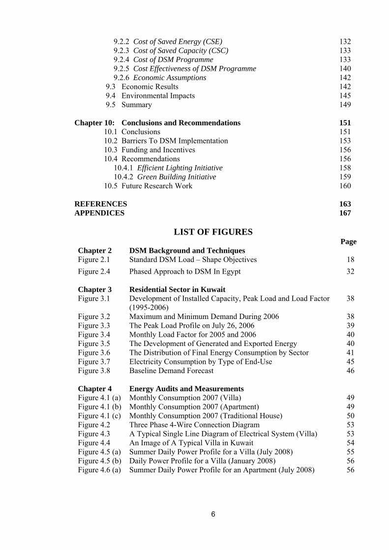
The outside air temperature plays also an important role in electricity monthly

demand variation. The monthly load factor for 2005 and 2006 is illustrated in Figure

3.4. It ranges between 77.6 and 81.6 % in winter and between 82.5 and 86.6% in

summer.

39

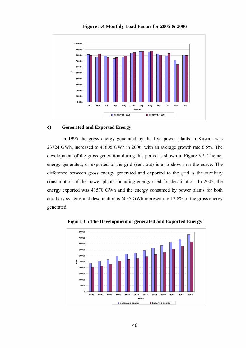
Figure 3.4 Monthly Load Factor for 2005 & 2006

0.00% 10.00% 20.00% 30.00% 40.00% 50.00% 60.00% 70.00% 80.00% 90.00%

100.00%

Jan Feb Mar Apr May June July Aug Sep Oct Nov Dec Months

%

Monthly LF, 2005 Monthly LF, 2006

c) Generated and Exported Energy

In 1995 the gross energy generated by the five power plants in Kuwait was

23724 GWh, increased to 47605 GWh in 2006, with an average growth rate 6.5%. The

development of the gross generation during this period is shown in Figure 3.5. The net

energy generated, or exported to the grid (sent out) is also shown on the curve. The

difference between gross energy generated and exported to the grid is the auxiliary

consumption of the power plants including energy used for desalination. In 2005, the

energy exported was 41570 GWh and the energy consumed by power plants for both

auxiliary systems and desalination is 6035 GWh representing 12.8% of the gross energy

generated.

Figure 3.5 The Development of generated and Exported Energy

0

5000

10000

15000

20000

25000

30000

35000

40000

45000

50000

1995 1996 1997 1998 1999 2000 2001 2002 2003 2004 2005 2006

Years

GW

h

Generated Energy Exported Energy

40

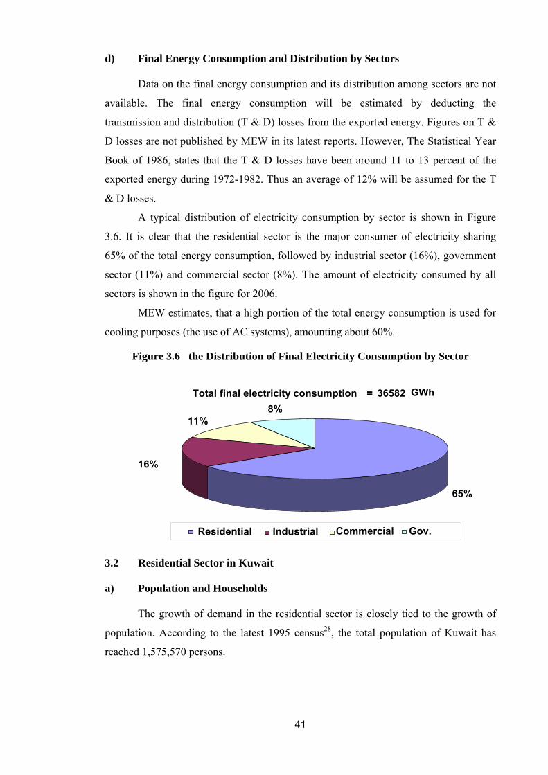
d) Final Energy Consumption and Distribution by Sectors

Data on the final energy consumption and its distribution among sectors are not

available. The final energy consumption will be estimated by deducting the

transmission and distribution (T & D) losses from the exported energy. Figures on T &

D losses are not published by MEW in its latest reports. However, The Statistical Year

Book of 1986, states that the T & D losses have been around 11 to 13 percent of the

exported energy during 1972-1982. Thus an average of 12% will be assumed for the T

& D losses.

A typical distribution of electricity consumption by sector is shown in Figure

3.6. It is clear that the residential sector is the major consumer of electricity sharing

65% of the total energy consumption, followed by industrial sector (16%), government

sector (11%) and commercial sector (8%). The amount of electricity consumed by all

sectors is shown in the figure for 2006.

MEW estimates, that a high portion of the total energy consumption is used for

cooling purposes (the use of AC systems), amounting about 60%.

Figure 3.6 the Distribution of Final Electricity Consumption by Sector

Total final electricity consumption = 36582 GWh

65%

16%

11% 8%

Residential Industrial Commercial Gov.

3.2 Residential Sector in Kuwait a) Population and Households

The growth of demand in the residential sector is closely tied to the growth of

population. According to the latest 1995 census28, the total population of Kuwait has

reached 1,575,570 persons.

41

According to the UN Department of Economic and Social Affairs/Population

Division, the total population of Kuwait reached 2.687 million persons in 2005, and the

average growth rate during the period 2000 – 2005 was 3.7%.

Kuwaiti national population is projected to increase at an average growth rate as

shown in Table 3.1.

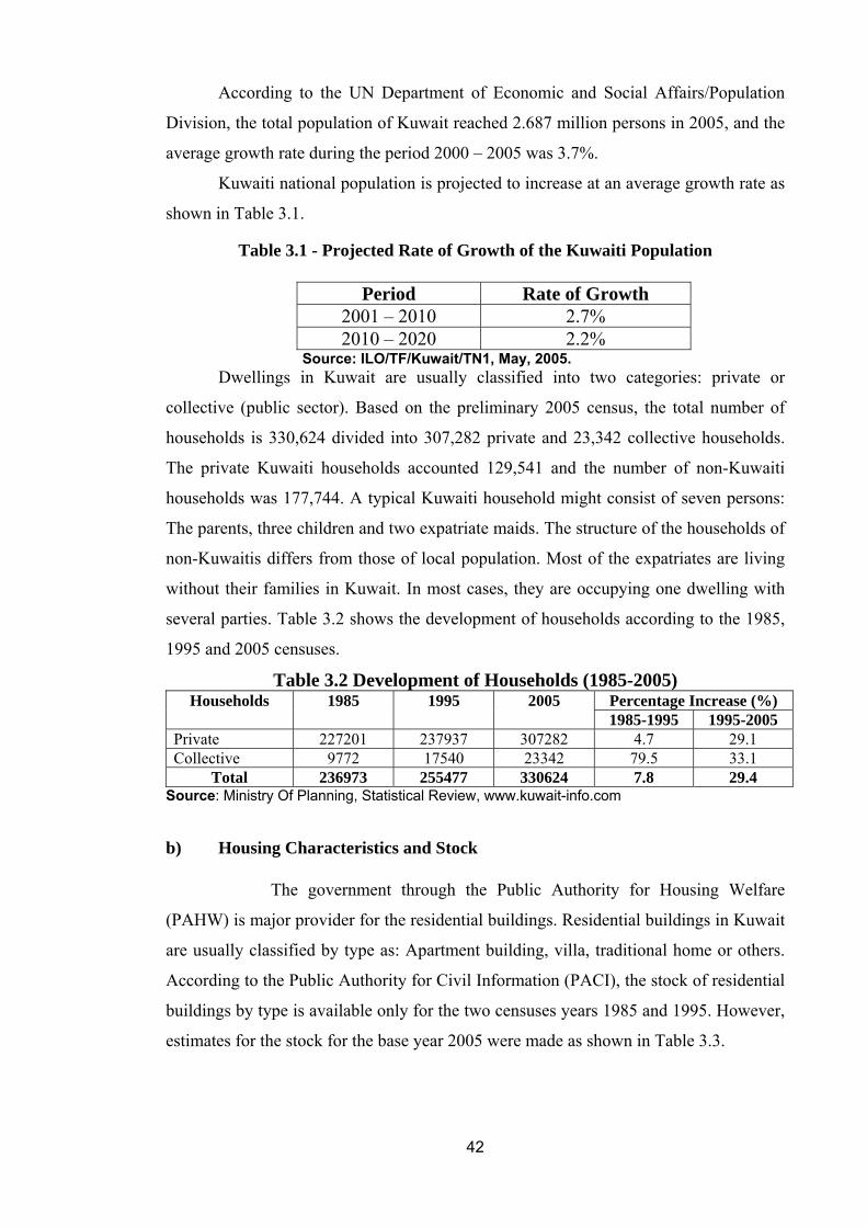
Table 3.1 - Projected Rate of Growth of the Kuwaiti Population

Period Rate of Growth 2001 – 2010 2.7% 2010 – 2020 2.2%

Source: ILO/TF/Kuwait/TN1, May, 2005. Dwellings in Kuwait are usually classified into two categories: private or

collective (public sector). Based on the preliminary 2005 census, the total number of

households is 330,624 divided into 307,282 private and 23,342 collective households.

The private Kuwaiti households accounted 129,541 and the number of non-Kuwaiti

households was 177,744. A typical Kuwaiti household might consist of seven persons:

The parents, three children and two expatriate maids. The structure of the households of

non-Kuwaitis differs from those of local population. Most of the expatriates are living

without their families in Kuwait. In most cases, they are occupying one dwelling with

several parties. Table 3.2 shows the development of households according to the 1985,

1995 and 2005 censuses.

Table 3.2 Development of Households (1985-2005) Percentage Increase (%) Households 1985 1995 2005 1985-1995 1995-2005

Private 227201 237937 307282 4.7 29.1 Collective 9772 17540 23342 79.5 33.1

Total 236973 255477 330624 7.8 29.4 Source: Ministry Of Planning, Statistical Review, www.kuwait-info.com b) Housing Characteristics and Stock

The government through the Public Authority for Housing Welfare

(PAHW) is major provider for the residential buildings. Residential buildings in Kuwait

are usually classified by type as: Apartment building, villa, traditional home or others.

According to the Public Authority for Civil Information (PACI), the stock of residential

buildings by type is available only for the two censuses years 1985 and 1995. However,

estimates for the stock for the base year 2005 were made as shown in Table 3.3.

42

Kind and size of household or dwellings in Kuwait determines to a large extent

residential electricity demand. The total stock of buildings in Kuwait is estimated at

approximately 237,000 conventional residential dwellings.

The estimates conducted by a German consulting office "Lahmeyer International

GmbH – The association of Engineering Partnership" in 1999, showed that dwelling

stock consists roughly of:

• 122,666 apartments (52%),

• 52,234 villas (22%)

• 30,450 traditional homes (13%)

• 31,664 other dwellings (13%) – other dwellings are mostly low-income

dwellings.

As shown in Table 3.3, the share of villas to the total dwelling stock reached

more than 60% in 2005.

Table 3.3 Types and Numbers of Dwellings29

Years Building 1985 1995 2005

Increase 1985-1995

(%)

Increase 1995-2005

(%) A- Dwellings Stock: Private 219042 234153 303045

(982.26%) 6.9 29.4

Collective 9801 17529 23354 (6.34%)

78.8 33.2

Vacant 33356 32763 35762 (9.71%)

- 1.8 9.2

Under Construction 6921 3129 6235 (1.69%)

- 54.8 99.3

Total 269120 287574 368396 (100%)

6.9 28.1

B- Type of Dwellings: Apartment 9959 9862 13579 - 0.1 37.7 Villa 53839 61870 104650 1.4 69.2 Traditional Home 33670 30969 31000 - 0.8 0 Others (*) 18661 17155 15800 - 0.8 - 0.8

Total 116129 119856 Source: Ministry Of Planning, Census and Statistical Sector, www.kuwait-info.com (*) Others include temporary buildings, chalets, buildings under construction, etc.

In reality, more than 50% of the Kuwaiti prefers to live in villas, while about

35% are living in traditional homes and only 15% are living in apartments.

43

Based on the data from the construction statistics30, the area of new villa ranges

between 500 and 900 m2, and the area of new apartments lie in the range of 150 to 180

m2.

Table 3.4 shows the classification of residential consumers according to ranges

of consumption in both private and apartment buildings as published in 1999.

Approximately half of the residential consumers in private dwellings (320,890

connections in 2005) consume less than 4000 kWh per month.

Table 3.4 Electricity Consumption of Residential Consumers31

Private Houses Apartment Buildings

Consumption (kWh/month)

Share in Number (%)

Share in Con-sumption (%)

Consumption (kWh/month)

Share in Number (%)

Share in Con-sumption (%)

1 – 4000 49 22 1 – 1250 45 18 4001 – 6000 21 20 1250 – 2500 42 46 6001 – 9000 18 26 2501 – 4200 9 17

> 9000 12 32 4201 – 6250 2 5 > 6250 2 13

Total 100 100 100 100 Source: Al-Qabas (Local Official Newspaper), Kuwait, 12 August, 1999. c) Electricity Tariff

Almost all consumers in Kuwait, including residential sector, are charged a flat

rate of 2 fils (≈ US¢ 0.6) per kWh of electricity, when in fact, the cost of producing

each kWh has been estimated at 14 to 26 fils, which means that electricity is subsidized

by 12 up to 24 fils per kWh.

During the last two decades, several proposals were made by MEW for tariff

increase however; the tariff modification was not implemented. 3.3 Energy Consumption by End-use Equipment

For successful implementation of DSM measures in the residential

sector, it is important to explore the hourly power consumption of electrical end-use

appliances on typical winter and summer days. Unfortunately, exact data for the

electricity consumption by end-use equipment is not available. According to the World

Bank study conducted in 1993, air conditioning systems accounted for 73% of the

residential consumption in 1989, and thus, that is equivalent to, at least, 47% (73% *

65%) of total final energy consumption (not counting the air conditioning load of other

44

consumer categories). This estimate is consistent with the recent data, provided by

MEW, pointing out that summer peak is almost double winter peak due to the load

required for AC.

Assuming the same share of AC consumption in the residential sector is still

valid for the present time, thus the amount of electrical energy used by AC equipment in

the whole sector is estimated as 17358 GWh.

Lighting comes in the second place, after AC, with respect to energy

consumption, since most of the Kuwaitis use chandeliers in their homes lighted with as

much as 12 to 24 lamps. The type of lamps used is most likely incandescent 40 or 60

Watt. The compact fluorescent lamps (CFLs) are not yet widespread in Kuwait.

Roughly, the breakdown of the electricity consumption by type of end-use

equipment could be estimated as shown in the pie chart below (Figure 3.7).

Figure 3.7 Electricity Consumption by Type of End-Use

70.0%

12.0%

6.0%

3.0% 2.5%4.0%

2.5%

Air Condition (Cooling)

Lighting

Refrigerator + Freezer

Washing

Water Heating

TV/Video

Misc.

3.4 Baseline Scenario and Demand Forecast

To determine the DSM potential for the residential sector, it is important

to establish a disaggregated base-line demand scenario of energy consumption and

demand forecasts. Currently, there are no publicly available energy consumption

forecasts that include end-use sector (residential, industrial and commercial)

breakdowns.

45

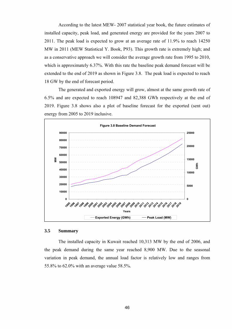
According to the latest MEW- 2007 statistical year book, the future estimates of

installed capacity, peak load, and generated energy are provided for the years 2007 to

2011. The peak load is expected to grow at an average rate of 11.9% to reach 14250

MW in 2011 (MEW Statistical Y. Book, P93). This growth rate is extremely high; and

as a conservative approach we will consider the average growth rate from 1995 to 2010,

which is approximately 6.37%. With this rate the baseline peak demand forecast will be

extended to the end of 2019 as shown in Figure 3.8. The peak load is expected to reach

18 GW by the end of forecast period.

The generated and exported energy will grow, almost at the same growth rate of

6.5% and are expected to reach 108947 and 82,388 GWh respectively at the end of

2019. Figure 3.8 shows also a plot of baseline forecast for the exported (sent out)

energy from 2005 to 2019 inclusive.

Figure 3.8 Baseline Demand Forecast

0

10000

20000

30000

40000

50000

60000

70000

80000

90000

1995

1996

1997

1998

1999

2000

2001

2002

2003

2004

2005

2006

2007

2008

2009

2010

2011

2012

2013

2014

2015

2016

2017

2018

2019

Years

MW

0

5000

10000

15000

20000

25000

GW

h

Exported Energy (GWh) Peak Load (MW)

3.5 Summary

The installed capacity in Kuwait reached 10,313 MW by the end of 2006, and

the peak demand during the same year reached 8,900 MW. Due to the seasonal

variation in peak demand, the annual load factor is relatively low and ranges from

55.8% to 62.0% with an average value 58.5%.

46

The gross energy generated in Kuwait in 2006 reached 47,605 GWh, with an

average growth rate 6.5% during the last decade. Around 13.3% of this energy is used

for desalination and auxiliary power and the rest is exported (sent out) to the grid.

During 2006, the final energy consumption was estimated at approximately

36,582 GWh, equivalent to the exported energy minus the transmission and distribution

losses (about 12%). The distribution of final energy consumption among sectors is

estimated at: 65% for residential sector, 16% industrial, 11% commercial and 8%

Government sector.

The residential sector is dominant in energy consumption due to the heavy use

of air conditioning systems in summer.

According to the latest 1995 census, the total population of Kuwait was

estimated at 1,575,570 persons, from which the Kuwaitis population is 653,616 persons

representing estimated population of Kuwait reached 2.687 million persons.

The data of 2005 census indicated that the number of households in Kuwait

reached 330,624 divided into 307,282 private and 23,342 collective households.

Residential buildings are usually classified into three categories: apartments, villas and

traditional buildings. The type of building defines, to large extend, electricity demand;

49% of private houses consume less than 4000 kWh/month, about 40% consume from

4000 to 9000 kWh/month, and 12% consume more than 9000 kWh/month. The area of

new villa ranges from 500 to 900 sq. meter, and the new apartment ranges from 150 to

180 sq. meters.

Almost all consumers in Kuwait, including residential sector, are charged flat

rate of 2 fils (≈ US¢ 0.6) per kWh, with minimum subsidy 12 fils per kWh. This very

low tariff is the main reason for the irrational use electrical energy.

Air conditioning systems are the major contributors of energy consumption in

residential buildings, where they share about 70% of the total consumption. Rough

estimates indicate that other end-use equipment in a typical Kuwaiti dwelling consume

electrical energy as follows: lighting (12%), refrigerators (6%), and other end-use

equipment (12%).

The peak load base-line demand forecast is expected to reach 20.8 GW by the

end of 2019, while the exported energy is expected to reach 82,368 GWh. These values

are important in evaluating the cumulative impacts of DSM programme(s).

47

Chapter 4

Energy Audits and Measurements

4.1 Introduction

This chapter includes the results of short audits (walk-through) and detailed

audits as well as measurements conducted on selected types of dwellings. Our aim, by

conducting these audits and measurements, is to identify the energy efficiency DSM

options in the selected samples. The samples were selected to represent, as much as

possible, the Kuwaiti residential sector behaviour. As mentioned earlier, the majority of

Kuwaiti dwellings are classified into three types: private villas, apartments and

traditional houses. Focusing on these types, we collected data for more than 50 villas,

50 apartments and about 20 traditional houses. The sources of data are mainly, the

Ministry of Planning, Statistical and Information Sector, Kuwait Institute for Scientific

Research (KISR), Ministry of Electricity and Water as well as site visits and a

questionnaire designed for this purpose. A model of the questionnaire is shown in

Appendix 4. Interviews with the owners helped in selecting the suitable dwellings for

detailed energy audit and the possibility of conducting measurements.

By screening the available data, we selected 10 villas, 10 apartments and 5

traditional houses that could be suitable candidates for detailed audits, including

measurements.

4.2 Results of Energy Audits

Through the energy, and in order to identify the DSM energy conservation

opportunities (ECOs), it is important to identify where and how the building uses

energy. For this purpose, we have to gather live information on the following:

• Monthly energy bills.

• Building construction, including area, type of insulation, windows, etc.

• End-use equipment with particular emphasis on air conditioning (A/C) and

lighting systems.

• Types, sizes, and, if possible, the average operating hours per day and/or week

for home appliances such as washing machines, water heaters, TV, etc.

• Occupancy rates.

48

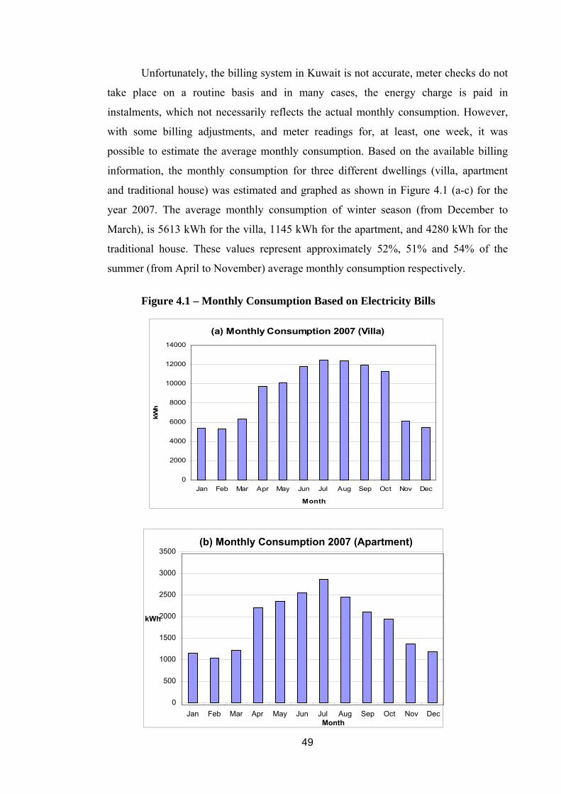
Unfortunately, the billing system in Kuwait is not accurate, meter checks do not

take place on a routine basis and in many cases, the energy charge is paid in

instalments, which not necessarily reflects the actual monthly consumption. However,

with some billing adjustments, and meter readings for, at least, one week, it was

possible to estimate the average monthly consumption. Based on the available billing

information, the monthly consumption for three different dwellings (villa, apartment

and traditional house) was estimated and graphed as shown in Figure 4.1 (a-c) for the

year 2007. The average monthly consumption of winter season (from December to

March), is 5613 kWh for the villa, 1145 kWh for the apartment, and 4280 kWh for the

traditional house. These values represent approximately 52%, 51% and 54% of the

summer (from April to November) average monthly consumption respectively.

Figure 4.1 – Monthly Consumption Based on Electricity Bills

(a) Monthly Consumption 2007 (Villa)

0

2000

4000

6000

8000

10000

12000

14000

Jan Feb Mar Apr May Jun Jul Aug Sep Oct Nov Dec

Month

kWh

(b) Monthly Consumption 2007 (Apartment)

500

1000

1500

2000

2500

3000

3500

0Jan Feb Mar Apr May Jun Jul Aug Sep Oct Nov Dec

Month

kWh

49

(c) Monthly Consumption 2007 (Traditional House)

0

1000

2000

3000

4000

5000

6000

7000

8000

9000

10000

Jan Feb Mar Apr May Jun Jul Aug Sep Oct Nov DecMonth

kWh

During audits process, emphasis was made on four major contributors in energy

consumption, specifically: building construction, air conditioning systems, lighting

systems, and end-use equipment.

• Building Construction:

Assessment of building construction details, such as the type of wall and roof

insulation was difficult, since the owner and/or occupants are not acquainted with such

issues. However, most of the windows in the audited dwellings are double-glazed with

low-e or reflective coated glass and either PVC or aluminium frames. Light coloured

walls and roofs are common in, almost, all surveyed dwellings, however, the lack of

shading is remarked in most of them.

• Air Conditioning Systems:

In most of the villas and traditional houses use air cooled packaged rooftop A/C

systems. For villas the total installed cooling capacity ranges from 40 refrigeration ton

(RT)1 to about 60 RT depending on the size of the villa. Slightly less capacity is used in

traditional houses. For apartments, split and window types are used. For the audited

dwellings, most of the A/C systems are installed more than 10 years ago, characterized

with low efficiency ranging 1.3 to 1.7 kW per ton, corresponding to an average

coefficient of performance (COP) around 2.5. Proper sizing of A/C systems as well as

energy performance will be investigated by simulation (Chapter 5).

1 1Refrigeration Ton = 3.516 kW

50

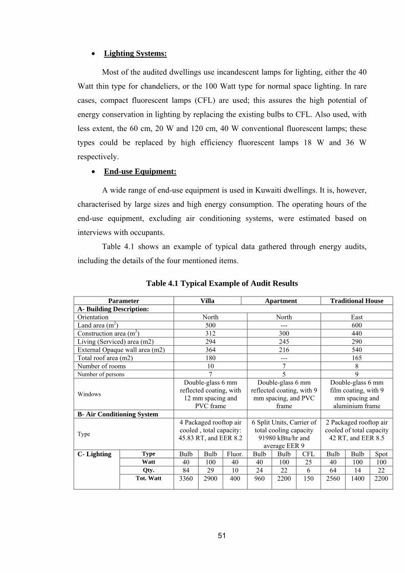
• Lighting Systems:

Most of the audited dwellings use incandescent lamps for lighting, either the 40

Watt thin type for chandeliers, or the 100 Watt type for normal space lighting. In rare

cases, compact fluorescent lamps (CFL) are used; this assures the high potential of

energy conservation in lighting by replacing the existing bulbs to CFL. Also used, with

less extent, the 60 cm, 20 W and 120 cm, 40 W conventional fluorescent lamps; these

types could be replaced by high efficiency fluorescent lamps 18 W and 36 W

respectively.

• End-use Equipment:

A wide range of end-use equipment is used in Kuwaiti dwellings. It is, however,

characterised by large sizes and high energy consumption. The operating hours of the

end-use equipment, excluding air conditioning systems, were estimated based on

interviews with occupants.

Table 4.1 shows an example of typical data gathered through energy audits,

including the details of the four mentioned items.

Table 4.1 Typical Example of Audit Results

Parameter Villa Apartment Traditional House

A- Building Description: Orientation North North East Land area (m2) 500 --- 600 Construction area (m2) 312 300 440 Living (Serviced) area (m2) 294 245 290 External Opaque wall area (m2) 364 216 540 Total roof area (m2) 180 --- 165 Number of rooms 10 7 8 Number of persons 7 5 9

Windows

Double-glass 6 mm reflected coating, with

12 mm spacing and PVC frame

Double-glass 6 mm reflected coating, with 9 mm spacing, and PVC

frame

Double-glass 6 mm film coating, with 9

mm spacing and aluminium frame

B- Air Conditioning System

Type

4 Packaged rooftop air cooled , total capacity: 45.83 RT, and EER 8.2

6 Split Units, Carrier of total cooling capacity

91980 kBtu/hr and average EER 9

2 Packaged rooftop air cooled of total capacity

42 RT, and EER 8.5

Type Bulb Bulb Fluor. Bulb Bulb CFL Bulb Bulb Spot Watt 40 100 40 40 100 25 40 100 100 Qty. 84 29 10 24 22 6 64 14 22

C- Lighting

Tot. Watt 3360 2900 400 960 2200 150 2560 1400 2200

51

Type

Refrigerators (2)

Refrigerators (1)

Refrigerators (2)

Consumption 88 + 79 = 167 kWh/m 86 kWh/m 54 + 74 = 128 kWh/m Type Clothes washer (2) Clothes washer (1) Clothes washer (2)

Consumption 43 + 45 = 88 kWh/m 48.5 kWh/m 64 + 66 = 130 kWh/m Type Water heaters (3) Water heaters (2) Water heaters (3)

Consumption 1x540 + 2x270 = 1080 kWh/m

360 + 240 = 600 kWh/m

1x540 + 2x360 = 1260 kWh/m

Type TV (2) TV (3) TV (3) Consumption Total: 223 kWh/m Total: 82 kWh/m Total: 72.6 kWh/m

Type Electric heaters (2) Electric heaters (2) Electric heaters (3) Consumption Total: 270 kWh/m Total: 240 kWh/m Total: 360 kWh/m

Type Others (Computers, VCR, Radio, etc.)

Others (Computers, VCR, Radio, etc.)

Others (Computers, VCR, Radio, etc.)

D- End-use Equipment

Consumption Total: 369 kWh/m Total: 64 kWh/m Total: 130 kWh/m

4.3 Results of Measurements

Measurements were carried out on samples of each of the dwellings type: a villa,

apartment and a traditional house. To obtain a full picture on the energy demand and

load profile, measurements were carried out using a demand analyzer: VIP –

SYSTEM-3.

The instrument is connected in 4-wire mode as shown in Figure 4.2. It records

on permanent basis the active and reactive powers, energy, power factor and harmonics.

It also measures the true root mean square (RMS) of voltage and current and calculates

the following parameters:

• Active power (kW)

• Reactive power (kVAR)

• Apparent power (kVA)

• True power factor (PF)

• Displacement power factor (dPF)

• Total harmonic distortion (THD) of voltage and current.

52

Figure 4.2 Three Phase 4-wires Connection Diagram

Measurements were carried for 10 villas, 10 apartments and 5 traditional houses

of different consumption categories. Periods of measurements ranges from 3 to 7 days,

including weekend in each period. Due to the high impact of weather conditions in

Kuwait on energy use and the heavy use of air conditioning systems in summer

measurements were carried out in winter (January 2008) when the air conditioners are

off, and in summer (July 2008) when all air conditioning systems are in peak operation.

Measurements were carried out on the main feeders on the 380 V voltage level,

supplying power to all loads in the dwelling. Figure 4.3 shows a typical electrical single

line diagram (SLD), for an audited villa.

Figure 4.3 a typical Single Line Diagram of Electrical System (Villa)

M a in C B

y

O utdoor G round Fl . Fi rst Fl . R oof A/C 1 A/ C 2 A/C 3

F r om Uti l it

L ight i ng (Plugs + L ight ) (Pl ugs + L ight )

380 V

53

Figure 4.4 an Image of a Typical Villa in Kuwait

Figures 4.5, 4.6 and 4.7 show the daily power demand profile for a villa,

apartment and traditional house respectively. The profiles are traced for both summer

(July 2008) and winter (January 2008). The results of measurements conducted in 25

facilities are summarized in the following Tables.

Table 4.2 Summary of Measured Parameters

(a) For Villas

Parameter Summer Winter Maximum Active Power (kW) 18.2 – 34 10.5 – 17.2

Average Active Power (kW) 12.99 – 17.6 5.6 – 7.06

Average Reactive Power (kVAR) 9.4 – 12.74 3.62 – 4.0

Average Power Factor 0.79 – 0.84 0.79 – 0.9

Average Line Voltage (V) 389.6 390.8

Average Daily Consumption (kWh) 312 – 422 134 – 169

(b) For Apartments

Parameter Summer (July)

Winter (January)

Maximum Active Power (kW) 5.8 – 10.4 2.8 – 4.7

Average Active Power (kW) 2.71 – 4.31 1.08 – 1.56

Average Reactive Power (kVAR) 1.75 – 3.12 0.58 – 1.21

Average Power Factor 0.79 – 0.89 0.79 – 0.9

Average Line Voltage (V) 382 387

Average Daily Consumption (kWh) 65 – 103 26 – 37

54

(c) For Traditional Houses

Parameter Summer (July)

Winter (January)

Maximum Active Power (kW) 18 – 24 5.6 – 13.5

Average Active Power (kW) 11.08 – 13.33 3.72 – 4.72

Average Reactive Power (kVAR) 6.46 – 8.0 2.11 – 2.29

Average Power Factor 0.79 – 0.89 0.79 – 0.9

Average Line Voltage (V) 383.5 390

Average Daily Consumption (kWh) 266 – 320 89 – 113

The large difference between summer and winter consumption is clear due to the

A/C cooling energy required. As indicated in Table 4.2, the ratio of average daily

demand in winter (January) relative to that in summer (July) ranges approximately from

35% to 40%.

Measurements in almost all dwellings showed low power factor, this is due to

air conditioners and fluorescent lamps as well as other electronic equipment. In Kuwait

no penalty charge is applied for low power factor.

Figure 4.5 (a) Summer Daily Power Profile for a Villa

(July 2008)

0,00

5,00

10,00

15,00

20,00

25,00

30,00

10:15 12:15 14:15 16:15 18:15 20:15 22:15 0:15 2:15 4:15 6:15 8:15

Time/Hrs

Active Power (kW)

55

Figure 4.5 (b) Daily Power Profile for a Villa (January 2008)

0,00

2,00

4,00

6,00

8,00

10,00

12,00

10:15 12:15 14:15 16:15 18:15 20:15 22:15 0:15 2:15 4:15 6:15 8:15

Time/Hrs

kW

Power Profile (kW)

Figure 4.6 (a) Summer Daily Power Profile for an Apartment (July 2008)

0,00

1,00

2,00

3,00

4,00

5,00

6,00

7,00

10:30 12:30 14:30 16:30 18:30 20:30 22:30 0:30 2:30 4:30 6:30 8:30

Time/Hr

Active Power (kW)

56

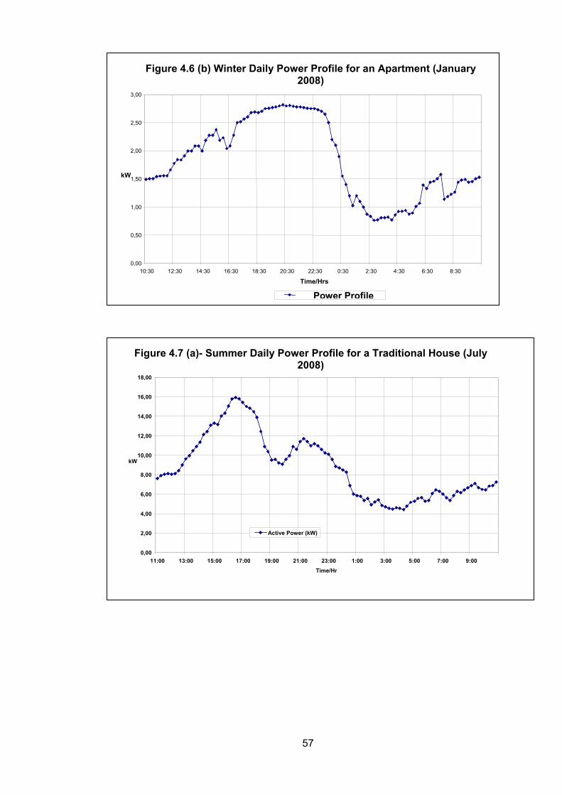
Figure 4.6 (b) Winter Daily Power Profile for an Apartment (January 2008)

0,00

0,50

1,00

1,50

2,00

2,50

3,00

10:30 12:30 14:30 16:30 18:30 20:30 22:30 0:30 2:30 4:30 6:30 8:30

Time/Hrs

kW

Power Profile

Figure 4.7 (a)- Summer Daily Power Profile for a Traditional House (July 2008)

0,00

2,00

4,00

6,00

8,00

10,00

12,00

14,00

16,00

18,00

11:00 13:00 15:00 17:00 19:00 21:00 23:00 1:00 3:00 5:00 7:00 9:00Time/Hr

kW

Active Power (kW)

57

0,00

1,00

2,00

3,00

4,00

5,00

6,00

7,00

8,00

9,00

11:00 13:00 15:00 17:00 19:00 21:00 23:00 1:00 3:00 5:00 7:00 9:00

Time/Hr

kW

Power Profile (kW)

Figure 4.7 (b)- Winter Daily Power Profile for a Traditional House (January 2008)

4.4 Summary

Data collection and detailed energy audits conducted for 25 Kuwaiti dwellings

(10 villas, 10 apartments and 5 traditional houses) during the first 8 months of year

2008 have revealed the following results:

• The average consumption, based on monthly bills and meter recordings, of the

three types of dwellings is approximately:

Winter Summer Villa (kWh/m) : 5613 8870 Apartment (kWh/m): 1145 2250 Traditional house (kWh/m): 4280 7925

That is the average winter consumption almost half that of summer

consumption.

• In data collection and walk-through audits, emphasis were made on the

following main components:

a) Building construction,

b) Air conditioning systems,

c) Lighting systems, and

d) End-use equipment.

58

• Through energy audits, the main DSM options identified are:

a) High efficiency lighting by replacing the existing fluorescent lamps to

CFL.

b) Measures related to air conditioning systems.

c) Measures related to end-use equipment.

These measures, as well as others, will be investigated through building simulation.

• The results of measurements for, at least, three days for each facility (including

weekend) have shown the following average electrical parameters:

Villa Apartment Tr. House - Average daily summer (July) demand (kW): 13-17.6 2.7-4.3 11-13.3 - Average daily winter (Jan.) demand (kW): 5.6-7 1.1-1.56 3.72-4.72 - Maximum daily summer (July) demand (kW): 18.2-34 5.8-10.4 18-24 - Maximum daily winter (Jan.) demand (kW): 10.5-17.2 2.8-4.7 5.6-13.5 - Average PF summer (July): 0.79-0.84 0.79-0.89 0.79-0.89 - Average PF winter (Jan.): 0.79-0.9 0.79-0.9 0.79-0.9

The ratio of average daily demand in peak winter (January) to the average daily

demand in peak summer (July) ranges approximately from 35% to 40%. This, of course,

is due to the high consumption of air conditioning systems.

59

CHAPTER 5

BUILDING SIMULATION

5.1 Introduction

In existing buildings, energy simulation is performed to analyze the energy

performance of a building dynamically and to understand the relationship between the

design parameters and energy use characteristics of the building.

From an energy point of view, a building is quite complex system. A particular

measure taken for energy conservation might influence the building and the energy end-

use of the building, as several measures might interact. This influence, and hence the

real energy conservation, might be difficult to foresee without analyzing the effect of

the measure taken on the energy end-use of the building in question as a whole. For

example, replacing normal incandescent lamps to compact fluorescent lamps (CFLs)

will have large effect on the air condition load, and hence on the overall energy savings.

Therefore, assumptions about energy conservation gained by a particular DSM measure

must include not only the conservation potential of the measure itself, but also its

influence on the total need for energy when the building is in normal use. This is a

fundamental prerequisite for achieving energy efficiency in reality.

Simulation process, including HAP, is performed sequentially in three

programmes. The first programme (called SPACES or LOADS) uses weather data, user

input regarding the characteristics of the building envelope, and the building's schedule

of occupancy in order to calculate the heating addition and/or cooling extraction rates

that occur in each building space. The energy performance of day-lighting, lighting,

domestic hot water and other end-use equipment are also calculated in SPACES. The

second programme (SYSTEM) uses the inputs of the first programme to calculate the

demand for ventilation air, electricity, etc., to maintain temperature and humidity set

points. In addition, control equipment, HVAC auxiliary equipment, and energy recovery

equipment are also evaluated within the SYSTEM programme. The final programme

(PLANT) simulates the behaviour of the primary HVAC system (boiler, chillers,

cooling towers, etc.) in meeting these demands and predicts the fuel or electrical energy

consumed.

60

5.2 Simulation Tool Used

The simulation programme used in research work is the Carriers Hourly

Analysis Programme (HAP). It is mainly used in the design and analysis for commercial

buildings; however, it is used successfully in residential applications. It has the

advantage of better user interface and default features. The HAP estimates the annual

energy consumption and energy costs for AC and non-AC energy consuming systems

associated with a particular building design, by simulating its operation for each of the

8760 hours in a year. It calculates load requirement for the building for each hour

depending on the difference between the internal and external gain/loss. Results of the

energy analysis are used to compare the energy use and energy costs of the actual

existing operation of the dwelling as it is (base-case) with the operation under

alternative DSM measures. Specifically, HAP performs the following tasks during

energy analysis:

• Simulates, on an hourly basis, the operation of all air conditioning systems in

the building.

• Simulates, on an hourly basis, the operation of non – AC systems, including

lighting and appliances.

• Uses results of the hour-by-hour simulations to calculate total annual energy

use and energy costs.

• Generates tabular and graphical reports of hourly, daily, monthly and annual

data.

All analysis work requires the same general five step procedure: 1) Problem Definition: First we have to define the scope and objectives of the energy

analysis, including the type of building, type and rates of systems and equipment

installed, and what alternate designs or energy conservation measures are being

compared in the analysis.

61

2) Gathering Data: Before energy simulations can be run, information about the

building, its environment, AC and non-AC equipment, and its energy prices must be

gathered. This step required extracting data from building plans, evaluating building

usage, studying AC system needs and acquiring utility rate schedules. Specific types

of information needed include:

• Hourly weather data for the building site: includes information on maximum

and minimum temperature, humidity, seasonal variations, etc.

• Building design parameters and description: includes information on

construction material, type of walls, roof, insulation, windows, glazing and

shading coefficients, infiltration, etc.

• Internal load characteristics determined by levels and schedules for

occupancy, lighting system, water heaters, office equipment, appliances and

machinery within the building.

• Data for AC equipment, controls and components to be used.

• Data for non-AC energy consuming equipment.

• Utility rate information for electric service used in the building (in our

analysis, electricity is the only source of energy used).

3) Entering Data into HAP: It is very important to define input data parameters

before using HAP, or any other simulation tool. Three building models from the

audited dwellings were selected to perform the simulation: a villa, an apartment and

a traditional house. The major components of energy simulation for each of these

models are shown in Figure 5.1. As shown in the figure, climatic data and building

construction details as well as end-use equipment are essential sources of

information for simulation process. The output of the HAP is in the form of energy

performance reports including energy consumption, costs, environmental emissions,

etc.

The data of the three dwellings description, air conditioning systems, lighting

and end-use equipment are shown in Table 5.1. Data entry included the following types:

a. Weather data is entered by loading a simulation weather file from the library

provided with the programme. For Kuwait city, the weather data is shown in

Appendix 4.

62

b. Geometric data is entered, either for the whole building or divided into zones.

All elements which affect heat flow in the space must be described, such as

walls, windows, doors, roofs, skylight, floors occupants, lighting, electrical

equipment, infiltration and partitions.

c. Air system data related to AC equipment used to provide cooling (in almost all

Kuwaiti dwellings, AC is off during winter). An air system serves one or more

zones. In our analysis, AC serves two zones (ground and first floors) for villa

and traditional house and three zones for apartment (reception, master bed

room and other bed rooms). The air systems typically used in the villas and

traditional houses is the package rooftop units and in the apartments are split

units of different ratings (see Table 4.1, Chapter 4).

d. Utility rate data is entered specifying the pricing rules for electrical energy.

MEW charges a flat tariff rate of 2 Fils (≈ 0.006 US$) per kWh to almost all

its residential consumers. MEW also states that the electricity production costs

have been about 14 Fils (0.042 US$) per kWh delivered to the customer. Thus,

the unit costs are 7 times higher than the average sales price. This means that

the amount of subsidy is 12 Fils (≈ 0.036 US$) per kWh. The utility rate

considered in this analysis is the minimum amount of subsidy, i.e. 12 fils (≈

US¢ 3.6) per kWh.

Figure 5.1 Major Components of Building Energy Analysis Simulation

Building Model

A/C Data, Lighting & End-use

Equipment

Control System Model

Building Construction

A/C System Model

Simulation System

Climate Data (Kuwait City)

Energy Performance

Reports

63

5.3 Simulation Scenarios and DSM Measures

For each selected type of dwellings, the HAP simulation process included five

DSM measures, in addition to, the base case. Table 5.1 (a) shows the input parameters

for the base case and Table 5.1 (b) shows the variations in input data according to DSM

selected option. Nine alternatives, including different DSM scenarios, were simulated as

follows:

• Alternative 1 - Base Case: Simulation is carried out for the base case scenario of each dwelling in its

actual existing condition. Input parameters shown in Table 5.1 for the base case are

based mainly on the results of detailed energy audits.

• Alternative 2 - DSM1: In almost all audited dwellings, the thermostat setting was put in the range

between 70 o F (21.1o C) to 75 o F (23.9 o C). In this scenario, a simple DSM measure is

applied by increasing thermostat setting from 75 o F (23.9 o C) to 78 o F (25.6 o C).

Interviews with occupants have shown that the new thermostat setting is convenient in

most cases.

• Alternative 3 – DSM2: In this alternative, it is assumed that high efficiency lighting is used by

replacing the existing incandescent lamps 40 W and 100 W to compact fluorescent

lamps (CFL), of rated power 7 W and 25 W respectively. All other building parameters

are kept the same as in the base case.

• Alternative 4 – (DSM1 + DSM2): In this alternative, Simulation is carried out assuming that the two energy

efficiency DSM options DSM1 and DSM2 are implemented simultaneously, the

aggregated sum of savings is evaluated.

64

• Alternative 5 – DSM3: Most of the existing air conditioning systems in the audited dwellings are not

efficient with energy efficiency ratios (EER) ranging from 7.5 to 9.5. In this alternative,

the simulation was carried out assuming that the A/C has been upgraded to a new type

more efficient with EER about 11.0. In this DSM option, it is assumed that all other

parameters are kept the same as in the base case.

• Alternative 6 – (DSM1 + DSM2 + DSM3): In this alternative, it is assumed that all three previous DSM measures are

applied simultaneously, and the accumulated energy savings are calculated.

• Alternative 7 – DSM4: This DSM option is usually applied for new buildings. It takes into

consideration the quality of roof and wall insulation. In this case, we assume that, the U-

value of the base case roof insulation: 1.266 W/m²K for villa, 0.613 W/m²K for

apartment, and 0.233 W/m²K for traditional house has been increased to 0.363 W/m²K,

0.392 W/m²K, and 0.169 W/m²K respectively. Moreover, the U-value of the base case

wall insulation has been upgraded from 1.266 to 0.346 W/m²K, from 0.613 to 0.392

W/m²K, and from 0.233 to 0.169 W/m²K for villa, apartment and traditional house

respectively. Also, the medium colour of the villa's roof is assumed to be upgraded to

light colour.

• Alternative 8 – DSM5: In this alternative, it is assumed that part or all the end-use equipment

(refrigerators, washing machines, water heaters, etc.) have been replaced by energy

efficient ones. Assuming 25% increase in end-use equipment efficiency, with respect to

the base case, simulation was carried out and the results are shown in the tables in

appendix 9.

• Alternative 9 – (Sum of DSM Options): This is the last alternative, in which it is assumed that all five DSM measures

are implemented and the aggregate savings were calculated as shown in the tables of

appendix 9.

65

Table 5.1 (a) Input Data For Building Simulation for the Base Case

Date: January 25, 2009 Dwelling Types:

Location: Kuwait City

Villa, Apartment and

Tr. House A. WEATHER DATA Latitude 29.2 Degree Elevation 180.0 ft Summer Design Dry Bulb Temp. 110.0 ºF Summer Coincident Wet Bulb Temp. 85.0 ºF Daily Temperature Range 25.0 ºF Winter Design Dry Bulb Temp. 45.0 ºF Atmospheric Clearance Number 1.0 Data Source Carrier Defaults Design Cooling Months March to November B. GENERAL DWELLING DATA DATA VILLA APARTMENT TR. HOUSE Floor (Living) Area (sq ft) 3358 2637 3100 Building Weight (lb/sq ft) 90 120 90 Avg. Ceiling Height (ft) 10.2 9.0 9.0 Roof Gross Area (sq ft) 1722 1000 1700 C. LIGHTING DATA Power Density (PD) 1.1 W / sq ft 0.8 W / sq ft 0.8 W / sq ft

Fixture Type Free hanging Recessed (Unvented) Free hanging

D. PEOPLE Occupancy (No. of persons) 7 4 7 Activity Level Zone 1 Sedentary Work Seated at Rest Seated at Rest Zone 2 Sedentary Work Seated at Rest Seated at Rest Zone 3 Seated at Rest E. AIR CONDITIONING INPUT DATA

Equipment class Packaged

Rooftop Units Split Air

Handling Units Packaged

Rooftop Units Air System Type VAV VAV VAV Number of Zones 2 3 2 Cooling T-stat (case 1) 78 0 F 78 0 F 78 0 F Supply Air Flow 49978.4 CFM 6985 CFM 23000 CFM Gross Cooling Capacity 550 MBH 153 MBH 500 MBH Design OAT 107 0 F 107 0 F 95 0 F Compressor & Fan Power 65 kW (8.5) 15.9 kW (9.6) 55 kW (9.1)

66

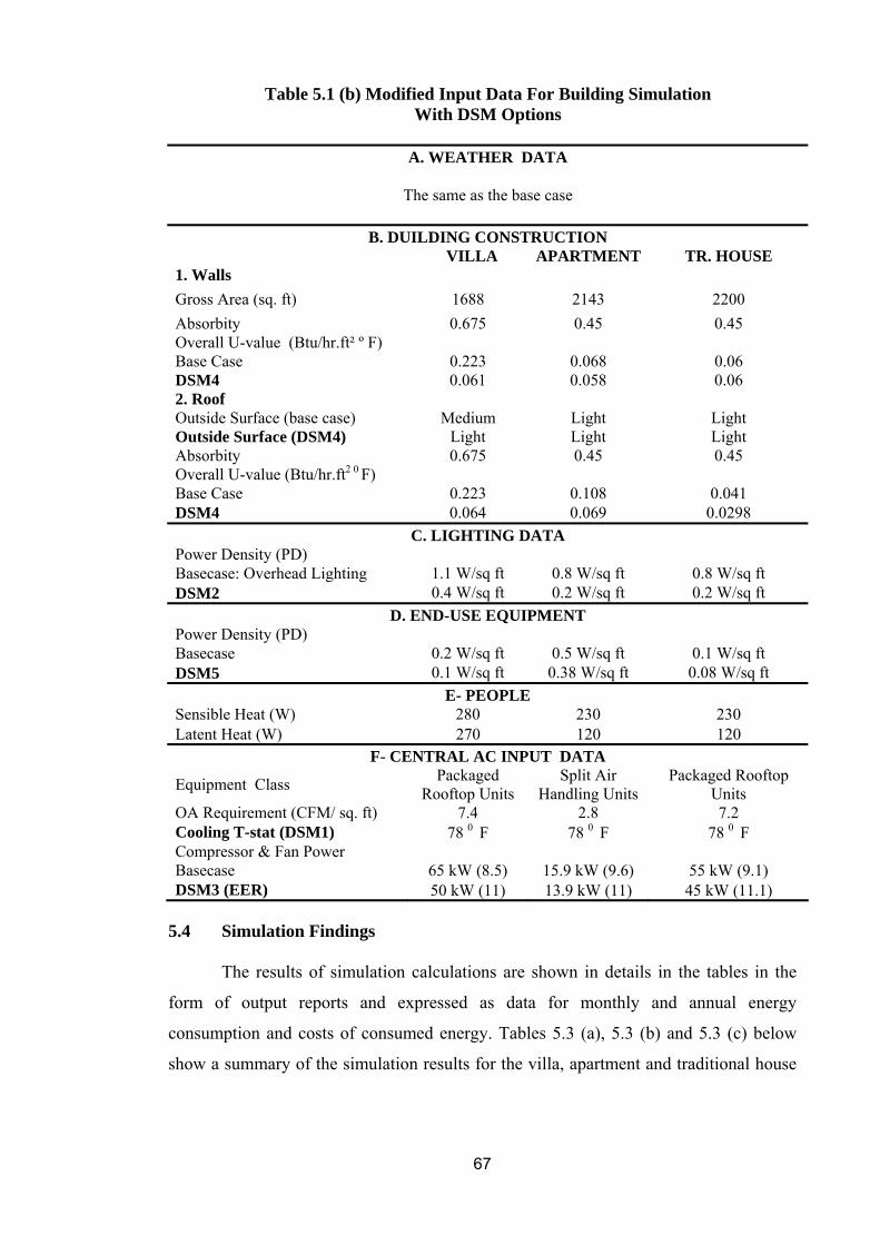
Table 5.1 (b) Modified Input Data For Building Simulation With DSM Options

A. WEATHER DATA

The same as the base case

B. DUILDING CONSTRUCTION

VILLA APARTMENT TR. HOUSE 1. Walls Gross Area (sq. ft) 1688 2143 2200 Absorbity 0.675 0.45 0.45 Overall U-value (Btu/hr.ft² º F) Base Case 0.223 0.068 0.06 DSM4 0.061 0.058 0.06 2. Roof Outside Surface (base case) Medium Light Light Outside Surface (DSM4) Light Light Light Absorbity 0.675 0.45 0.45 Overall U-value (Btu/hr.ft2 0 F) Base Case 0.223 0.108 0.041 DSM4 0.064 0.069 0.0298

C. LIGHTING DATA Power Density (PD) Basecase: Overhead Lighting 1.1 W/sq ft 0.8 W/sq ft 0.8 W/sq ft DSM2 0.4 W/sq ft 0.2 W/sq ft 0.2 W/sq ft

D. END-USE EQUIPMENT Power Density (PD) Basecase 0.2 W/sq ft 0.5 W/sq ft 0.1 W/sq ft DSM5 0.1 W/sq ft 0.38 W/sq ft 0.08 W/sq ft

E- PEOPLE Sensible Heat (W) 280 230 230 Latent Heat (W) 270 120 120

F- CENTRAL AC INPUT DATA

Equipment Class Packaged Rooftop Units

Split Air Handling Units

Packaged Rooftop Units

OA Requirement (CFM/ sq. ft) 7.4 2.8 7.2 Cooling T-stat (DSM1) 78 0 F 78 0 F 78 0 F Compressor & Fan Power Basecase 65 kW (8.5) 15.9 kW (9.6) 55 kW (9.1) DSM3 (EER) 50 kW (11) 13.9 kW (11) 45 kW (11.1)

5.4 Simulation Findings

The results of simulation calculations are shown in details in the tables in the

form of output reports and expressed as data for monthly and annual energy

consumption and costs of consumed energy. Tables 5.3 (a), 5.3 (b) and 5.3 (c) below

show a summary of the simulation results for the villa, apartment and traditional house

67

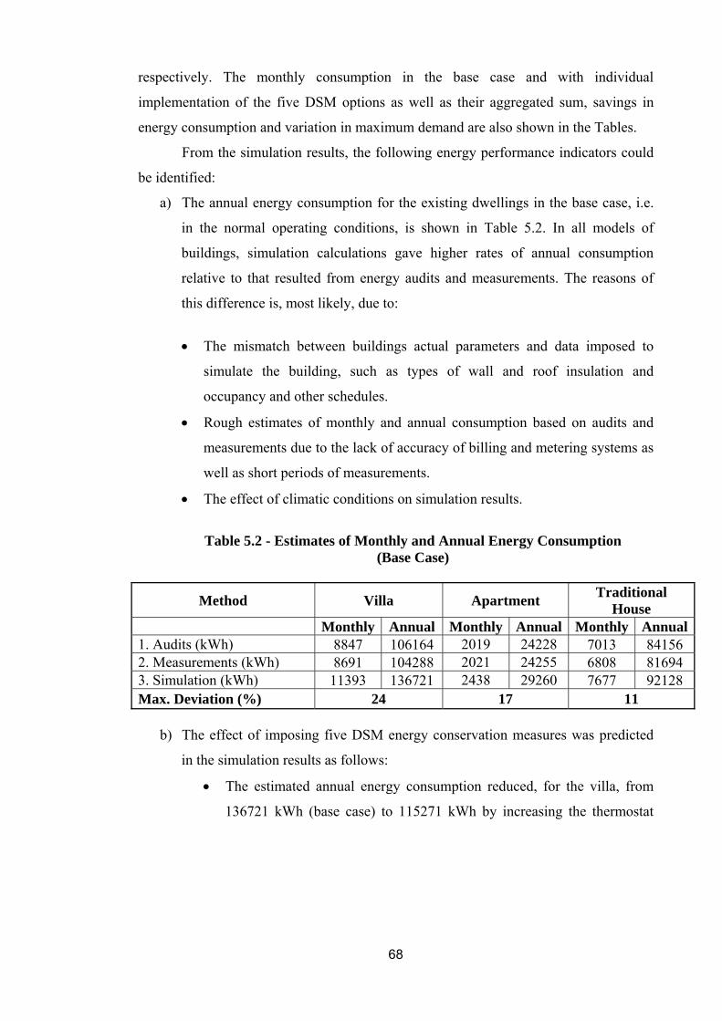
respectively. The monthly consumption in the base case and with individual

implementation of the five DSM options as well as their aggregated sum, savings in

energy consumption and variation in maximum demand are also shown in the Tables.

From the simulation results, the following energy performance indicators could

be identified:

a) The annual energy consumption for the existing dwellings in the base case, i.e.

in the normal operating conditions, is shown in Table 5.2. In all models of

buildings, simulation calculations gave higher rates of annual consumption

relative to that resulted from energy audits and measurements. The reasons of

this difference is, most likely, due to:

• The mismatch between buildings actual parameters and data imposed to

simulate the building, such as types of wall and roof insulation and

occupancy and other schedules.

• Rough estimates of monthly and annual consumption based on audits and

measurements due to the lack of accuracy of billing and metering systems as

well as short periods of measurements.

• The effect of climatic conditions on simulation results.

Table 5.2 - Estimates of Monthly and Annual Energy Consumption

(Base Case)

Method Villa Apartment Traditional House

Monthly Annual Monthly Annual Monthly Annual1. Audits (kWh) 8847 106164 2019 24228 7013 84156 2. Measurements (kWh) 8691 104288 2021 24255 6808 81694 3. Simulation (kWh) 11393 136721 2438 29260 7677 92128 Max. Deviation (%) 24 17 11

b) The effect of imposing five DSM energy conservation measures was predicted

in the simulation results as follows:

• The estimated annual energy consumption reduced, for the villa, from

136721 kWh (base case) to 115271 kWh by increasing the thermostat

68

setting from 75 0 F (23.9 0 C) to 78 0 F (25.6 0 C)2. Similarly for the

apartment and traditional house, the annual consumption reduced from

28908 kWh and 92129 kWh to 22977 kWh and 77588 kWh respectively.

• Calculations show that annual energy consumption reduced, for the villa,

from 136721 kWh (base case) to 113967 kWh by replacing the

incandescent lamps of rated power 40 W and 100 W to CFL of rated

power 7 W and 25 W respectively. This energy efficiency measure is

called DSM2. As a conservative approach, only 75% of the overhead

lamps are replace giving a light power density (LPD) of 0.2 W/ft2 instead

of an existing value of 0.8 W/ft2. Similarly simulation results for the

apartment and traditional house indicated that annual consumption was

reduced from 28908 kWh and 92129 kWh to 24131 kWh and 74619

kWh respectively.

• By upgrading the existing AC systems having EER ranges from 8.5 to

9.6 to more efficient systems with EER about 11, the reduction in energy

consumption reached 22918 kWh, 2918 kWh and 12261 kWh for the

villa, apartment and traditional house respectively.

• The simulation of the fourth DSM measure, which assumes the use of

better wall and roof insulation resulted a reduction in annual energy

consumption reached 3144 kWh for the villa, 156 kWh for the apartment

and 2821 kWh for the traditional house.

2 This is a conservative approach, since the actual setting of thermostat is usually less than 23 o C

69

70

• The last simulated DSM option assumes the use of more efficient end-

use equipment. The predicted reductions in annual consumption are:

6305 kWh for villa, 442 kWh for apartment and 2473 kWh for the

traditional house.

• Simultaneous implementation of the above five DSM measures indicated

an aggregated sum of energy reduction reached 89311 kWh (65.3%) for

the villa, 12912 kWh (44.7%) for the apartment and 43860 kWh (47.6%)

for the traditional house.

The analysis of the above results, as well as, other DSM policy options will be

discussed in Chapter 6.

Table 5.3 (a) - Villa Monthly Simulation Results Base Case DSM1 DSM2 DSM3 DSM4 DSM5 DSM Total

Energy Cons. (kWh) Energy Cons. (kWh) Energy Cons.

(kWh) Energy Cons. (kWh) Energy Cons. (kWh) Energy Cons. (kWh) Energy Cons. (kWh)

Month Max. Demand

(kW) A/C Non

A/C

Max. Demand

(kW) A/C Non A/C

Max. Demand

(kW) A/C Non

A/C

Max. Demand

(kW) A/C Non A/C

Max. Demand

(kW) A/C Non A/C

Max. Demand

(kW) A/C Non A/C

Max. Demand

(kW) A/C

Non A/C

Jan 9,10 0 3194 9,10 0 3194 4,7 0 2047 9,1 0 3194 9,1 0 3194 8,6 0 2860 4 0 1447 Feb 9,10 0 2869 9,10 0 2869 4,7 0 1833 9,1 0 2869 9,1 0 2869 8,6 0 2572 4 0 1299 Mar 12,00 484 3150 10,60 264 3150 6,4 287 2005 11,3 372 3150 13,1 541 3150 11,3 426 2827 4,6 191 1425 Apr 20,90 3242 3086 18,40 2252 3086 13,9 2645 1976 18,2 2494 3086 18,7 2478 3086 20,1 3093 2764 7,7 786 1398 May 41,50 12001 3194 35,60 9228 3194 32,2 10709 2047 34 9231 3194 33,3 8112 3194 40,3 11660 2860 15 3505 1447 Jun 50,00 16510 3045 42,90 13014 3045 40,3 15080 1935 40,6 12700 3045 38,7 10760 3045 48,8 16138 2733 18,1 5037 1377 Jul 57,90 19564 3194 49,80 15583 3194 47,8 18037 2047 46,6 15049 3194 43,9 12602 3194 56,6 19161 2860 21,1 6072 1447 Aug 65,10 22461 3153 55,90 18018 3153 54,3 20747 2006 52,2 17277 3153 49,3 14554 3153 63,7 22020 2830 23,9 7124 1426 Sep 57,20 16274 3083 49,10 12860 3083 46,9 14838 1975 46,1 12519 3083 43,9 10847 3083 55,9 15904 2761 20,9 5114 1397

Oct 37,10 8766 3186 31,90 6634 3186 29,7 7692 2044 30,7 6743 3186 30 6265 3186 36 8488 2852 13,6 2636 1444

Nov 9,10 0 3045 9,10 0 3045 4,7 0 1935 9,1 0 3045 9,1 0 3045 8,6 0 2733 4 0 1377

Dec 9,10 0 3219 9,10 0 3219 4,7 0 2082 9,1 0 3219 9,1 0 3219 8,6 0 2874 4 0 1461

AVG. 31,51 8275 3118 28 6488 3118 24 7503 1994 26 6365 3118 26 5513 3118 31 8074 2794 12 2539 1412

Total 99303 37418 77853 37418 90035 23932 76385 37418 66159 37418 96890 33526 30465 16945

Total 378,10 136721 330,60 115271 290,30 113967 316,10 113803 307,30 103577 367,10 130416 140,90 47410

Saving 0 0 47,50 21450 87,80 22754 62,00 22918 70,80 33144 11,00 6305 237,20 89311

% Sav. 0% 0% 12,6% 15,7% 23,2% 16,6% 16,4% 16,8% 18,7% 24,2% 2,91% 4,6% 62,7% 65,3%

DSM1 Thermostat Resetting from 75 to 78 o F

Btu

DSM2 Replacing 80% of Incandescent Bulbs to CFL

DSM3 Upgrade A/C Equipment to Efficient Units with EER = 11

DSM4 Increase Wall and Roof Insulation (R from 4 to 16 hr.ft2 .O F) /

DSM5 Use Energy Efficient End-Use Equipment

DSM Aggregate Implementation of All DSM Options (∑DSM1 to DSM5)

71

Table 5.3 (b) - Apartment Monthly Simulation Results

Base Case DSM1 DSM2 DSM3 DSM4 DSM5 DSM Total

Energy Cons. (kWh)

Energy Cons. (kWh)

Energy Cons. (kWh)

Energy Cons. (kWh)

Energy Cons. (kWh) Energy Cons. (kWh) Energy Cons.

(kWh) Month Max.

Demand (kW) A/C

Non A/C

Max. Demand

(kW) A/C Non A/C

Max. Demand (kW) A/C

Non A/C

Max. Demand

(kW) A/C Non A/C Max. Demand

(kW) A/C Non A/C

Max. Demand (kW) A/C

Non A/C

Max. Demand

(kW) A/C Non A/C

Jan 1,9 0 485 1,9 0 485 0,9 0 241 1,9 0 485 1,9 0 485 1,8 0 462 0,8 0 218

Feb 1,9 0 438 1,9 0 438 0,9 0 218 1,9 0 438 1,9 0 438 1,8 0 417 0,8 0 197

Mar 2,1 70 485 2 49 485 1 50 241 2,1 61 485 2,2 71 485 2,1 69 462 0,9 43 218

Apr 4,3 666 469 3,6 384 469 2,8 542 233 4 582 469 4,3 665 469 4,1 655 447 1,9 237 211

May 9,1 2737 485 7,6 1964 485 7,2 2469 241 8,3 2393 485 9,1 2723 485 9 2713 462 4,9 1484 218

Jun 11,4 3890 469 9,5 2917 469 9,3 3591 233 10,2 3401 469 11,3 3866 469 11,2 3863 447 6,5 2286 211

Jul 13,2 4651 485 11 3547 485 11,1 4333 241 11,8 4066 485 13,1 4618 485 13 4622 462 7,8 2817 218

Aug 15,2 5531 485 12,8 4281 485 13 5177 241 13,6 4836 485 15,2 5492 485 15 5499 462 9,2 3421 218

Sep 12,8 3775 469 10,6 2832 469 10,9 3477 233 11,4 3300 469 12,7 3745 469 12,6 3748 447 7,5 2207 211

Oct 8,1 1879 485 6,7 1294 485 6,5 1655 241 7,3 1642 485 8 1863 485 8 1858 462 4,3 934 218

Nov 1,9 0 469 1,9 0 469 0,9 0 233 1,9 0 469 1,9 0 469 1,8 0 447 0,8 0 211

Dec 1,9 0 485 1,9 0 485 0,9 0 241 1,9 0 485 1,9 0 485 1,8 0 462 0,8 0 218

AVG. 7,0 1933,3 475,8 6,0 1439,

0 475,8 5,5 1774,

5 236,4 6,4 1690,

1 475,8 7,0 1920,3 475,8 6,9 1918,9 453,3 3,9 1119,1 213,9 Sub-Tot. 23199,0

5709,0

17268,0 5709,0

21294,0

2837,0

20281,0 5709,0 23043,0 5709,0 23027,0 5439,0 13429,0 2567,0

Total 28908,0 22977,0 24131,0 25990,0 28752,0 28466,0 15996,0

Saving 0,0 0,0 1,0 5931,0 1,5 4777,0 0,6 2918,0 0,0 156,0 0,1 442,0 0,0 12912,0

% Sav. 0,0% 0,0% 14,8% 20,5% 22,0% 16,5% 8,9% 10,1% 0,0% 0,5% 1,4% 1,5% 43.9% 44,7%

DSM1 Thermostat Resetting from 75 to 78 o F

DSM2 Replacing 80% of Incandascent Bulbs to CFL

DSM3 Upgrade A/C Equipment to Efficient Units with EER = 11

DSM4 Increase Wall and Roof Insulation (R from 4 to 16 hr.ft2 .O F) / Btu

DSM5 Use Energy Efficient End-Use Equipment

DSM Aggregate Implementation of All DSM Options (∑DSM1 to DSM5)

72

73

Table 5.3 (c) Traditional House Monthly Simulation Results

Base Case DSM1 DSM2 DSM3 DSM4 DSM5 DSM Total

Energy Cons. (kWh)

Energy Cons. (kWh)

Energy Cons. (kWh)

Energy Cons. (kWh)

Energy Cons. (kWh)

Energy Cons. (kWh) Energy Cons. (kWh) Month

Max. Demand

(kW) A/C Non A/C

Max. Demand

(kW) A/C Non A/C

Max. Demand

(kW) A/C Non A/C

Max. Demand

(kW) A/C Non A/C

Max. Demand

(kW) A/C Non A/C

Max. Demand

(kW) A/C Non A/C

Max. Demand

(kW) A/C Non A/C

Jan 6 0 1800 6 0 1800 2,4 0 968 6 0 1800 6 0 1800 5,8 0 1677 2,2 0 844

Feb 6 0 1619 6 0 1619 2,4 0 867 6 0 1619 6 0 1618 5,8 0 1508 2,2 0 757

Mar 8 412 1783 6,7 263 1783 3,2 263 949 7,9 340 1783 8,1 371 1783 7,7 306 1664 2,9 218 830

Apr 15,1 2527 1740 13,5 1824 1740 9,8 2027 934 13,7 2090 1740 15,1 2403 1740 14,8 2369 1621 6,5 970 815

May 30,5 8794 1800 26,3 6911 1800 23,7 7733 968 26,3 7275 1800 30,2 8404 1800 30,1 8597 1677 15,8 4557 844

Jun 37,2 11949 1721 32 9560 1721 29,7 10760 915 31,8 9885 1721 36,8 11425 1721 36,7 11806 1606 19,9 6554 800

Jul 42,5 13949 1800 36,4 11243 1800 34,9 12676 968 36 11540 1800 41,9 13390 1800 42 13879 1677 23,5 7842 844

Aug 48,1 15867 1781 41,2 12840 1781 40 14429 949 40,6 13127 1781 47,4 15271 1781 47,5 15816 1662 27 8993 829

Sep 41,3 11399 1742 35,3 9109 1742 34,1 10203 935 35 9430 1742 40,7 11003 1742 40,8 11280 1623 23,1 6252 816

Oct 27,6 6085 1807 23,6 4691 1807 21,2 5199 970 23,7 5034 1807 27,2 5895 1807 27,1 5892 1684 14,4 2993 847

Nov 6 0 1721 6 0 1721 2,4 0 915 6 0 1721 6 0 1721 5,8 0 1606 2,2 0 800

Dec 6 0 1833 6 0 1833 2,4 0 991 6 0 1833 6 0 1833 5,8 0 1706 2,2 0 864

AVG. 22,9 5915,2 1762,3 19,9 4703,4 1762,3 17,2 5274,2 944,1 19,9 4893,4 1762,3 22,6 5680,2 1762,2 22,5 5828,8 1642,6 11,8 3198,3 824,2

Total 70982 21147 56441 21147 63290 11329 58721 21147 68162 21146 69945 19711 38379 9890

Total 92129 77588 74619 79868 89308 89656 48269

Saving 0 0 2,9 14541 5,7 17510 2,9 12261 0,2 2821 0,4 2473 11,0 43860

% Sav. 0% 0,0% 12,9% 15,8% 24,8% 19,0% 12,9% 13,3% 1,1% 3,1% 1,6% 2,7% 48,3% 47,6%

DSM1 Thermostat Resetting from 75 to 78 o F

Btu

ment

M5)

DSM2 Replacing 80% of Incandescent Bulbs to CFL

DSM3 Upgrade A/C Equipment to Efficient Units with EER = 11

DSM4 Increase Wall and Roof Insulation (R from 4 to 16 hr.ft2 .O F) /

DSM5 Use Energy Efficient End-Use Equip

DSM Aggregate Implementation of All DSM Options (∑DSM1 to DS

5.5 Summary

Three types of audited dwellings - villa, apartment and traditional house - were

selected for computer simulation. The tool used for simulation is the Carrier's Hourly

Analysis Programme. Data imposed for simulation are gathered from actual results of

detailed energy audits. Very limited building parameters were assumed based on market

trends, such as the type of wall and roof insulation. Energy simulation is aimed

primarily to evaluate the performance of the building and calculate the amount of saved

energy under different DSM measures. Matching with audit and measurements is also

an important issue to be investigated by simulation process.

The first simulation was carried out for the three dwellings in the base case

condition; in which the performance of the building is examined under its actual

existing condition and energy use. The simulation process was then repeated for the

following five DSM energy conservation measures:

1. Thermostat resetting from 75 0 F (23.9 0 C) to 78 0 F (25.6 0 C).

2. Replacement of about 80% of the incandescent lamps of rated power 40 W and

100 W to CFL of rated power 7 W and 25 W respectively..

3. Upgrading existing AC systems to more efficient types with EER = 11, instead

of 8.5 – 9.5 currently used.

4. The use of high insulation material for walls and roofs.

5. Upgrading the existing end-use equipment (refrigerators, washing machines,

water heaters, etc.) with more efficient ones.

Other simulation scenarios were carried out including simultaneous

implementation of "DSM1 + DSM2" and "DSM1 + DSM2 + DSM3", as well as the

simultaneous implementation of all five DSM options five options as illustrated in

Appendix 10.

Simultaneous implementation of the first three DSM options achieved an energy

saving of 49.7%, 43.8% and 43.1% of the base case consumption for the villa,

apartment and traditional house respectively; while the implementation of all five DSM

options achieved savings in the base case annual consumption equal to 65.3%, 44.7%

and 47.6% respectively.

74

Chapter 6

Analysis of Potential DSM Options

6.1 Introduction

The results of energy audits discussed in Chapter 4, and energy simulation

carried out on three dwelling types: a villa, apartment and traditional house, through

HAP programme and presented in Chapter 5, have shown attractive potentials for

energy efficiency improvement and savings opportunities through the application of

several of DSM energy efficiency measures. These results and the results of detailed

energy audits as well as the potential applications of other DSM measures need further

analysis.

The objective of this analysis is to identify the recommended portfolio of DSM

energy conservation measures. The analysis will cover not only the identified

technological DSM measures, but also the selection of the most appropriate policy

measures suitable for the condition of Kuwait.

6.2 Analysis of Audit and Simulation Results

The energy performance of the selected dwellings based on detailed audits,

measurements and simulation is discussed in this section.

6.2.1 Base Case Condition

The base case represents the actual existing energy performance of the audited

and simulated types of dwellings. With reference to Table 5.2, Chapter 5, the annual

energy consumption based on audit and simulation results was estimated for each

dwelling type as: from 104 to 136 MWh for villa, from 24 to 29 MWh for apartment

and from 82 to 92 MWh for traditional house. These rates of consumption indicate the

following:

• The overall per capita consumption ranges from 10500 to 12850 kWh (the

average for Kuwait is approximately 12900 kWh). This rate of consumption is

extremely high and represents about 5 times the world average of electricity

consumption (IEA statistics).

75

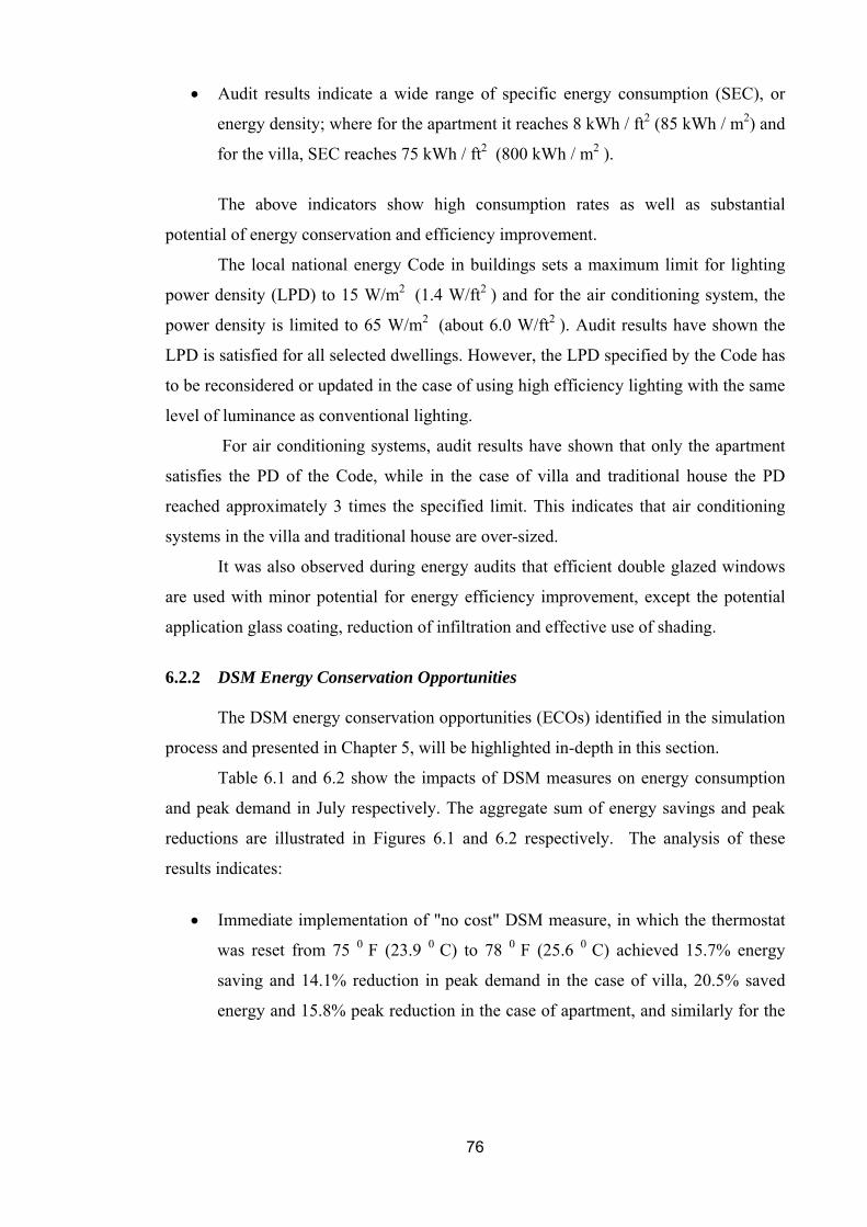
• Audit results indicate a wide range of specific energy consumption (SEC), or

energy density; where for the apartment it reaches 8 kWh / ft2 (85 kWh / m2) and

for the villa, SEC reaches 75 kWh / ft2 (800 kWh / m2 ).

The above indicators show high consumption rates as well as substantial

potential of energy conservation and efficiency improvement.

The local national energy Code in buildings sets a maximum limit for lighting

power density (LPD) to 15 W/m2 (1.4 W/ft2 ) and for the air conditioning system, the

power density is limited to 65 W/m2 (about 6.0 W/ft2 ). Audit results have shown the

LPD is satisfied for all selected dwellings. However, the LPD specified by the Code has

to be reconsidered or updated in the case of using high efficiency lighting with the same

level of luminance as conventional lighting.

For air conditioning systems, audit results have shown that only the apartment

satisfies the PD of the Code, while in the case of villa and traditional house the PD

reached approximately 3 times the specified limit. This indicates that air conditioning

systems in the villa and traditional house are over-sized.

It was also observed during energy audits that efficient double glazed windows

are used with minor potential for energy efficiency improvement, except the potential

application glass coating, reduction of infiltration and effective use of shading.

6.2.2 DSM Energy Conservation Opportunities

The DSM energy conservation opportunities (ECOs) identified in the simulation

process and presented in Chapter 5, will be highlighted in-depth in this section.

Table 6.1 and 6.2 show the impacts of DSM measures on energy consumption

and peak demand in July respectively. The aggregate sum of energy savings and peak

reductions are illustrated in Figures 6.1 and 6.2 respectively. The analysis of these

results indicates:

• Immediate implementation of "no cost" DSM measure, in which the thermostat

was reset from 75 0 F (23.9 0 C) to 78 0 F (25.6 0 C) achieved 15.7% energy

saving and 14.1% reduction in peak demand in the case of villa, 20.5% saved

energy and 15.8% peak reduction in the case of apartment, and similarly for the

76

traditional house 15.8% and 14.3% respectively. This option is very attractive

since it is simple and has an immediate payback period.

• It was clear from energy audits that most of lighting lamps used in all dwellings

are normal incandescent bulbs of rated power 100 W and 40 W. By replacing

these lamps to CFL of rated power 25 W and 7 W respectively, the potential

energy savings ranges from 16.5% to 19% and peak reduction from 14.5% to

16.8% as shown in Tables 7.1 and 7.2. Simulation results indicate a reduction of

approximately 9% in A/C consumption due to the implementation of this option.

• Simultaneous implementation of the above two DSM options has a potential

energy savings reached 38.5% for the villa, 37.1% for the apartment and 33.7%

for the traditional house.

• In the third DSM measure, we assumed the possibility of upgrading air

conditioning system to new more efficient with energy efficiency ratio about 11

instead of 8.5 – 9.0 in the base case. The achieved energy savings ranges from

10% to 16% and peak demand reduction ranges from 1.6% to 1.9%.

• The fourth DSM option assumes the use of better roof and wall insulation. As

predicted from simulation results, the amount of energy savings depends on the

U-value of the insulating material and the colour of walls and roofs. For

example, in the case of villa, light coloured roof achieved more than 20%

savings in energy.

• In the fifth DSM option, it was assumed that the end-use appliances, mainly the

refrigerators, washing machines, TV sets, and water heaters are replaced with

high efficiency ones (25% increase in efficiency). Savings in energy achieved

ranges from 1.5% to 4.6% and in peak demand reduction from 0.2% to 2.2%.

It is important to emphasize that the last two DSM options are usually

implemented for new buildings, however, the last option could be implemented in

the existing buildings when buying new appliance.

• The scenario of combining all five DSM options was run by the simulation

giving an attractive potential aggregate saving as follows:

For the villa: 65.3% saved energy and 47.6% reduction in peak demand.

For the apartment: 44.7% saved energy and 39.5% reduction in peak demand.

77

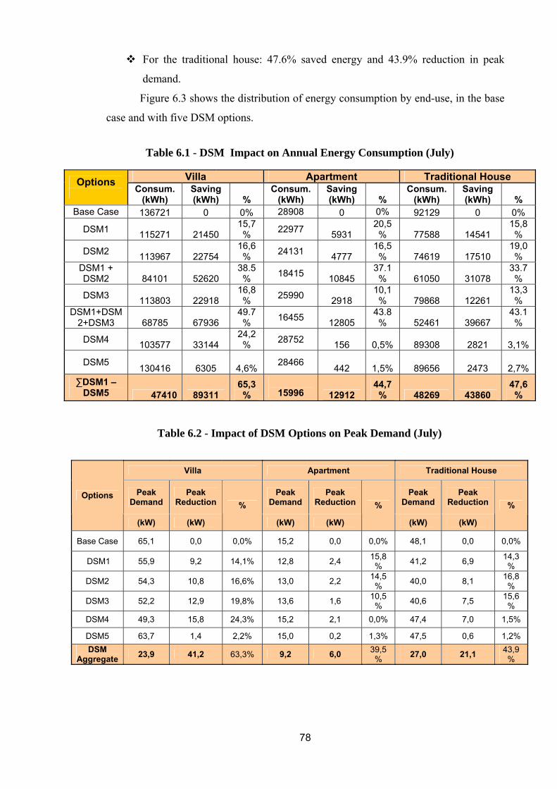
For the traditional house: 47.6% saved energy and 43.9% reduction in peak

demand.

Figure 6.3 shows the distribution of energy consumption by end-use, in the base

case and with five DSM options.

Table 6.2 - Impact of DSM Options on Peak Demand (July)

Table 6.1 - DSM Impact on Annual Energy Consumption (July)

Villa Apartment Traditional House

Peak Demand

Peak Reduction

Peak Demand

Peak Reduction

Peak Demand

Peak Reduction

Options

(kW) (kW)

%

(kW) (kW)

%

(kW) (kW)

%

Base Case 65,1 0,0 0,0% 15,2 0,0 0,0% 48,1 0,0 0,0%

DSM1 55,9 9,2 14,1% 12,8 2,4 15,8% 41,2 6,9 14,3

%

DSM2 54,3 10,8 16,6% 13,0 2,2 14,5% 40,0 8,1 16,8

%

DSM3 52,2 12,9 19,8% 13,6 1,6 10,5% 40,6 7,5 15,6

% DSM4 49,3 15,8 24,3% 15,2 2,1 0,0% 47,4 7,0 1,5%

DSM5 63,7 1,4 2,2% 15,0 0,2 1,3% 47,5 0,6 1,2% DSM

Aggregate 23,9 41,2 63,3% 9,2 6,0 39,5% 27,0 21,1 43,9

%

Villa Apartment Traditional House Options Consum.

(kWh) Saving (kWh) %

Consum. (kWh)

Saving (kWh) %

Consum. (kWh)

Saving (kWh) %

Base Case 136721 0 0% 28908 0 0% 92129 0 0%

DSM1 115271 21450 15,7% 22977 5931

20,5% 77588 14541

15,8%

DSM2 113967 22754 16,6% 24131 4777

16,5% 74619 17510

19,0%

DSM1 + DSM2 84101 52620

38.5% 18415 10845

37.1% 61050 31078

33.7%

DSM3 113803 22918 16,8% 25990 2918

10,1% 79868 12261

13,3%

DSM1+DSM2+DSM3 68785 67936

49.7% 16455 12805

43.8% 52461 39667

43.1%

DSM4 103577 33144 24,2% 28752 156 0,5% 89308 2821 3,1%

DSM5 130416 6305 4,6% 28466 442 1,5% 89656 2473 2,7% ∑DSM1 –

DSM5 47410 89311 65,3%

15996 12912

44,7% 48269 43860

47,6%

78

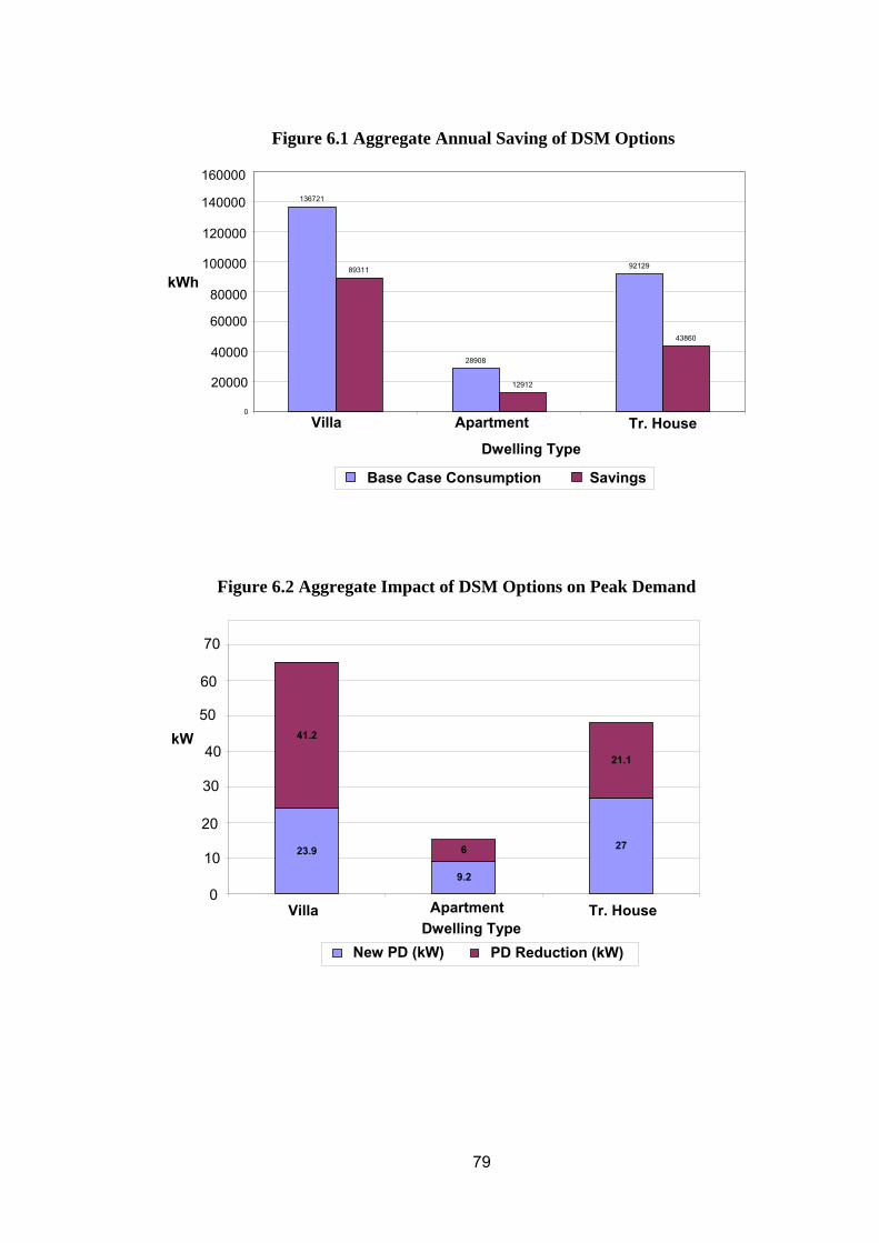
Figure 6.1 Aggregate Annual Saving of DSM Options

136721

28908

92129 89311

12912

43860

0

20000

40000

60000

80000

100000

120000

140000

160000

Villa Apartment Tr. House

Dwelling Type

Base Case Consumption Savings

kWh

Figure 6.2 Aggregate Impact of DSM Options on Peak Demand

23.9

9.2

27

41.2

6

21.1

0

10

20

30

40

50

60

70

Villa Apartment Tr. House Dwelling Type

kW

PD Reduction (kW) New PD (kW)

79

Figure 6.3 Distribution of Total Consumption by End-Use

80

6.3 Portfolio of DSM Technology Options

For further research analysis aiming to evaluate the overall DSM impact on the

national level, it is necessary to prepare a list, or portfolio, of potential DSM

opportunities that can, at the end on any DSM programme, can fulfil maximum energy

savings and optimum peak demand reduction on the national level.

In this section, I shall propose a portfolio of DSM options based on energy

audits, simulation process as well as the current condition in Kuwait related to

electricity use and tariff.

The DSM portfolio will consist of two categories, technological and policy. The

technological options are the five options evaluated by simulation process and

illustrated in Figure 7.4. Policy DSM options will be proposed based on the condition in

Kuwait and world experience.

6.4 Selection of DSM Policy Options

Based on the experience of many countries and energy situation in Kuwait, the

following two important policy DSM measures may have a potential energy savings and

peak demand reduction.

1. Increase of electricity tariff.

2. Energy Efficiency labels and standards for residential end-use appliances.

A brief description of these two DSM options is given below. 6.4.1 Increase of Electricity Tariff

MEW charges a flat tariff rate of 2 Fils (≈ 0.006 US$) per kWh to almost all its

residential consumers. Only owners of beach cabins (chalets) have to pay 10 Fils ( ≈

0.03 US$) per kWh. The low tariff rates have been in effect for more than 40 years. On

the other hand, MEW states that the electricity production costs have been about 14 Fils

( ≈ 0.042 US$) per kWh delivered to the customer. Thus, the unit costs are 7 times

higher than the average sales price. This means that the amount of subsidy is 12 Fils ( ≈

0.036 US$) per kWh accounting about 86% of the electricity costs.

This condition might give the consumer of electricity the impression that electric

power is available free of charge and electric energy is a cheap product, not necessary to

be consumed in an efficient manner. Such a low tariff rate is one of the most important

81

barriers to energy saving behaviour and to the introduction of energy efficiency DSM

technologies.

In September 1999, a new tariff proposal was submitted by MEW. The proposal

includes multi-part block rates for residential consumers and different tariffs for

commercial and industrial consumers and beach cabins. The proposal suggests that the

tariff rate for private consumers should be increased by 125% on average. Structure and

rates of proposed residential tariff are described in Table 6.3. For both private houses

and apartment buildings, the rates are divided into four blocks based on the average of

monthly consumption. Price increase may reach 400% of the current price in case of

consumption higher than 12000 kWh per month as shown in Table 6.3. For apartments,

separate meters system is proposed in this tariff, one for non A/C loads and one for A/C

as described in the table 6.3. Private houses with consumption less than 6000

kWh/month and apartments with less than 1500 kWh/month, the tariff will remain

unchanged; only consumers with high consumption will be affected. These consumers

usually can afford higher tariff and have a high savings potential.

Table 6.3 Proposed Electricity Tariffs for Residential Consumers

Apartment Building Private

House Separate Meters

Sep. Meters for non- A/C

Central A/C Meter

Current Prices

(Fils/kWh)

Proposed Price

(Fils/kWh)

Proposed Increase

(%)

1 – 6000 1-1500 1-600 1-900 2 2 0% 6001-9000 1501-

3000 601-1200 901-1700 2 4 100%

9001-12000 3001-6000

1201-2400 1701-3600 2 6 200%

Consumption

blocks in kWh

> 12000 > 6000 > 2400 > 3600 2 10 400% Average 2 4.5 * 125%

* Average price based on the assumption that 70% of the consumers are in the lower two consumption brackets which pay an average price of 3 Fils/kWh, and that 30% pay an average of 8 Fils/kWh.

The tariff proposal has to be approved by the Council of Ministers and National

Assembly in year 2000, however, it is still not yet approved facing a strong opposition

from consumers who have been used to low electricity prices for more than a

generation. The proposed tariff structure does not include two important tariff systems,

which are already applied in many countries:

• The Time Of Use (TOU) tariff, and

• Capacity charge tariff.

82

6.4.2 Energy Efficiency Labels and Standards

An energy efficiency standard is a regulation that prescribes minimum energy

performance (that is, the maximum energy use) of an energy-using product (most

commonly, household appliances, lighting products and other energy-consuming

equipment). Energy efficiency labels are information labels attached to manufactured

products indicating the product's Energy efficiency rating or estimated annual energy

use in order to provide consumers with the data necessary to make an informed

purchase. Appliance energy efficiency labelling and standards can be a primary force in

the creation of stronger markets for energy-efficient goods and services. By gradually

eliminating low-cost, inefficient appliance models and by stimulating the development

of more efficient technologies, labels and standards increase a country’s overall energy

efficiency.

Based on the experience of many developing countries such as China, India and

Algeria in this field, successful implementation of appliance labelling and efficiency

standards in Kuwait can yield significant results.

Consumers need access to information about how their homes or businesses use

energy, what energy – saving opportunities are open to them, and which products are

energy- efficient and cost-effective choices. Energy - efficiency labels can play an

important role in this consumer education.

For improving the efficiency of appliances, the most effective measures have

generally been mandatory energy – efficiency standards applied to manufacturers. Many

countries notably Canada, UK, China, the United States, Australia, Indonesia and

Thailand, have established mandatory standards for a variety of appliances, most

commonly refrigerators and air conditioners. Other countries have voluntary standards.

Developing countries and less developed countries have often drawn on the established

standards of other countries in developing their national standards.

83

Figure 6.4 – Portfolio of Proposed DSM Options

---------------------------------------------------------------------------------------------------------- 6.5 Summary

Based on detailed energy audits, results of HAP simulation, and the

consumption trends as well as electricity tariff structure in Kuwait, seven DSM options

are proposed in the DSM portfolio, five of them are technological measures and two are

policy measures.

These technological measures are characterized briefly as follows:

• Increasing thermostat setting point from 75 0 F (23.9 0 C) to 78 0 F

(25.6 0 C), could achieve a potential energy saving of, at least, 15% and peak

demand reduction of 14% relative to the base case consumption.

Technological DSM Options

Efficient A/C Equipment

Thermostat Setting

High Efficiency Lighting

Roof & Wall Insulation

Efficient End-Use Equipment

Policy DSM Options

Tariff Increase

Labels and Standards

84

• Replacement of conventional incandescent lamps with energy efficient CFLs of

self ballasted and "screw" type design may achieve a potential savings of 16.5%

in energy consumption and 15% in peak demand. This option gives a reduction

in A/C consumption estimated at 9%.

• Upgrading the existing A/C equipment to more efficient ones with EER > 11

instead of 8.5 or 9. The results indicate potential savings in energy consumption

16.8%, 10.1% and 13.3% for the villa, apartment and traditional house

respectively. The corresponding reduction in peak demand is 19.8%, 10.5% and

15.6% respectively.

• In case of simultaneous implementation of the first and second DSM options,

the amount of aggregated sum of energy saved reached 38.5%, 37.1% and

33.7% for the villa, apartment and traditional house respectively. Assuming

simultaneous implementation of the three DSM options, the total amount of

saving as reported by simulation reached: 49.7% for villa, 43.8% for apartment

and 43.1% for traditional house.

• The use of good wall insulation (DSM4) and the use of efficient end-use

equipment (DSM5) may achieve energy savings and reduction in peak demand

as shown in Tables 6.1 and 6.2. These two options are suitable for new

construction. As shown in Table 6.1 and 6.2, relatively, large amount of saving

is achieved in the villa by changing the walls and roof colour from "medium" to

"light" and using wall insulation with U-value = 0.346 W / m²K instead of

1.363 W / m²K.

Where as the two policy options are tariff increase and energy efficiency labels

and standards.

85

Chapter 7

Evaluation and Ranking of DSM Options

7.1 Introduction

In Chapters 5 and 6, a combination of technological and policy DSM measures

have been identified as potential opportunities to achieve the main goal of reducing

energy consumption and peak demand. These DSM measures include the following:

Thermostat setting (DSM1).

High efficiency lighting (DSM2).

Efficient air conditioning equipment (DSM3).

Roof and wall insulation (DSM4).

Efficient end-use equipment (DSM5).

Tariff increase (DSM6).

Labels and standards (DSM7).

The future penetration of these measures and their actual energy/power

reductions are dependent on many uncertain factors, such as end-use technology

development, market conditions, investment cost, customer acceptance and preference,

etc. These uncertainties are considered by specifying a number of possible scenarios

based on experts experience and their opinion on future economic and technological

developments.

For any new DSM programme design, it is important to define what are the most

cost-effective and suitable DSM measures and which one has the first priority in

programme implementation. In this Chapter, the Analytic Hierarchy Process (AHP) will

be used to evaluate the seven identified DSM measures and put them in priority order.

The Chapter includes an illustrative example and the steps of calculations. At the end of

the Chapter a priority list of the seven DSM options will be provided.

7.2 Criteria for Evaluation and Ranking

The criteria of evaluation the identified DSM options, on the sector level are

complex and non-homogeneous. The presence of several non-homogeneous criteria in a

multi-criteria decision making process requires a tool which is able to compare each of

86

the options intelligently. In our research, we use the Analytic Hierarchy Process (AHP)

or the Eigen-Vector Method (EVM), to help in setting priorities and making the best

decision with respect to both qualitative and quantitative aspects. AHP is a powerful

and flexible decision making process, that could be applied for any proposed DSM

programme, when decision about priorities is required. The AHP technique32, is based

on expert's opinion and mathematical analysis, is applied to estimate uncertain DSM

impacts on future electricity demand. Uncertainty is addressed with the use of discrete

probability estimates of the occurrence of the different scenarios. The probability

assignments are completed by pair-wise comparison of these scenarios and the Eigen-

value analysis. Then, the expected penetration level and unit impact are computed using

those probability weighted value. In order to determine the potential capacity and

energy cost savings due to DSM effects, the estimated impacts are used to investigate

the effect on the load duration pattern and integrated into supply-side planning process

by using the new load duration curve model.

7.2.1 The Analytic Hierarchy Process (AHP)

The formulation of the decision hierarchy is a critical step in the AHP process

because it effectively frames the problem and analysis in question. It uses a top down

approach and involves decomposing the problem into a hierarchy of interrelated

decision elements: goal, evaluation criteria and solution alternatives. Figure 7.1 shows a

three level hierarchy for selecting an appropriate DSM implementation strategy. At the

top of the hierarchy is the final goal which is defined as "Energy Savings and Peak

Demand Reductions" in the present context. The factors, or criteria, that affect the

choice of the best strategy are divided into six generic groups: Saved energy, peak

demand reduction, investment cost, payback period, penetration rate and technology

acceptance. In order to judge the relative importance of each criterion, we have to define

the rating intensity scales for each criterion as shown in Table 8.1. Each criterion has a

maximum weight of 9 and minimum of 1, divided into five scores as follows 9, 7, 5, 3

and 1. For example, the "payback period" criterion, will take the score 9 if it is

immediate or very short (as in the case of thermostat setting), and the scores 7, 5, 3 and

1 for short (from 1 to 2 years), medium (from 2 to 4 years), long (from 4 to 5 years) and

very long (> 5 years) payback periods respectively. The proposed weights and scores

87

shown in Table 7.1 are based on the world experience in DSM projects implementation

and in-depth interviews with experts in the field. Three experts, one from KISR33 and

two independent consultants having a long experience in DSM34,35

The third level consists of the DSM alternatives identified to satisfy the overall

decision goal. Arranging the goal, criteria and alternatives in this manner allows the

decision maker(s) to visualize the complex relationships inherent in the situation and

assess the importance of each issue at each level.

7.3 Features of Identified DSM Options

In order to reduce the risk of Uncertainty, and to facilitate the pair-wise

comparisons used in the AHP process, we shall try to emphasize the main features of

each DSM alternative and predict its characteristics in terms of the criteria given in

Table 7.1. This overview is mainly based on the results of audits, simulation as well as

successful DSM programmes implemented in developing countries. Based on these

features and interview with experts, the score of each DSM alternative is estimated as

shown in Table 7.2. The problem of uncertainty may be clear with respect to some

criteria, such as "penetration rate" and "technology acceptance". This problem is

minimized, as much as possible, by taking the minimum scores as a conservative

approach. Table 7.2 shows also a brief description of the technological DSM options.

Regarding regulatory options (tariff increase and labels and standards), we shall try to

assess its potential impact on energy consumption and peak demand as discussed in

different resources36, 37 Since the two policy options are not evaluated by simulation

process, so we shall try, through the following assessment to estimate the potential of

these options quantitatively as could be applied in Kuwait.

88

Table 7.1 Hierarchy Evaluation Criteria of DSM Options

Weight Criteria Definition Value For

1. Saved Energy Expressed as the amount of saved energy in kWh or as a percentage of total annual energy consumption of the dwelling. Criteria weight is linearly proportional to the amount of energy saved

1 3 5 7 9

< 10% (Very low) 10 – 20% (Low) 20 – 30% (Medium) 30 – 40% (High) > 40% (Very high)

2. Peak Demand Reduction

The of kW reduction in peak demand. It is maximum when coincides with the national peak and minimum if it is out of peak.

1 3 5 7 9

< 10% (Very low) 10 – 20% (Low) 20 – 30% (Medium) 30 – 40% (High) > 40% (Very high)

3. Investment Cost Defined as the investment cost for DSM measure implementation. It ranges from "No cost" to Very high cost.

1 3 5 7 9

Very high cost High cost Medium cost Low cost No Cost/Very low cost

4. Payback Period The simple payback period (PB)is defined as: cost PB Period = Net annual savings The shorter PB period, the most cost-effective DSM option.

1 3 5 7 9

> 5 years (Very long) 4 – 5 years (Long) 2 – 4 years (Medium) 1 – 2 years (Short) < 1 year (Very short)

5. Penetration Level

The penetration level represents the potential spreading of the DSM option in the assigned sector. The target of any DSM programme is to achieve 100% penetration by the end of the project.

1 3

Total capital

5 7 9

1 - 5% per year 5 – 10% per year 10 – 20% per year 20 – 30% per year > 30% per year

6. Technology Acceptance

It is important in any DSM programme design and implementation is not to select sophisticated technology that could not be promoted and accepted by the people. The contribution of local manufacturing in the technology applied is also important.

1 3

Low. Acceptance Medium Acceptance High Acceptance 5 Very High Acceptance 7 Full Acceptance 9

Source: Weight are proposed based on consultations with experts in DSM and designed to applicable in the AHP process.33,34,35

89

7.3.1 Impact of Tariff Increase

Tariff increase normally leads to a reduction in energy consumption. The short-

run prices elasticity of electricity consumption tends to be in the range of – 0.1 to - 0.2,

i.e. a tariff increase by 1% results in a consumption decrease by 0.1%. The effect of

tariff changes increases in the long-run, when consumers have more possibilities to

adapt their behaviour, therefore, long-run prices elasticity are higher than short-run

elasticity: in the range of – 0.2 to – 0.337.

In 1987, a study performed by KISR to assess the impact of alternative

electricity tariff on: energy consumption, equity for consumers and profitability for

producers, government subsidy and macro-economic effects. The study was only

concerned with the energy savings effect and did not estimate the effect on peak load.

To estimate demand functions for residential consumption, KISR used a

combination of time series and cross section data. Cross section data was used to

estimate the income elasticity of demand, while the time series data served to estimate

the price elasticity of demand. Short-term price elasticity was found to be in the order of

- 0.09 and medium-term elasticity (two to five years) in the order of - 0.30.

7.3.2 Energy Efficiency Standards and Labelling (EES&L)

The policy of energy efficient standards and labelling (EES & L) for end-use

equipment has now been applied in over 60 countries. Strong efficiency policies for

residential equipment used to be the near exclusive domain of industrialized economies,

especially the United States, European Union and Japan. However, this situation has

changed significantly with the development of policies, especially EES&L programmes.

In the 15 years between 1990 and 2005, the number of such programmes worldwide has

increased from 12 to over 60 (S. Wiel and J.E. McMahon 2005), including many

developing countries. The growth in the number of EES&L programmes indicates that

developing country governments are increasingly concerned with controlling Energy

90

Consumption and also that they view the experience of programmes in industrialized

countries as having been successful. Indeed, there have been notable successes.

For example, standards already written into law in USA are expected to reduce

residential sector consumption and carbon dioxide emissions by 8-9% by 2020 (Meyers,

McMahon, McNeil et al. 2003). Another study indicates that policies in all OECD

countries will likely reduce residential electricity consumption 12.5% in year 2020

compared to if no policies had been implemented to date (IEA 2003). Studies of impacts

of EES&L programmes already implemented in developing countries are rare, but there

a few encouraging examples. Mexico, for example, implemented its first minimum

Efficiency Performance Standards (MEPS) on four major products in 1995. By 2005,

only ten years later, standards on these products alone were estimated to have reduced

annual national electricity consumption by 9% (Sanchez, McNeil et al. 2007). Many

developing countries, including Kuwait, still have no efficiency policy regimes in place,

and therefore have a high technical potential. Many have EES&L for only a few

products or otherwise behind the world's best practices. For these reasons, a large effort

should be done to understand demand trends, performance characteristics of existing

appliances and the improvement potential in Kuwait.

Mandatory energy performance standards are important because they contribute

positively to a nation's economy and provide relative certainty about the outcome (both

timing and magnitude).

Labels also contribute positively to a nation's economy and increase the

awareness of the energy-consuming public. Labelling programmes are designed to

provide consumers with information, which enables them to compare the energy

efficiency of the different appliances on sale. They aim at modifying the selection

criteria of consumers by drawing their attention to the energy consumption of household

appliances. Labelling programmes, however, cannot sufficiently transform the market

and are usually completed by minimum performance standards in the great majority of

countries.

91

92

The household appliances, selected under this study, that need to be standardized

under an EES&L programme are based on the appliance share in household energy

consumption. As in most countries, the EES&L programme could be implemented

gradually in Kuwait by selecting specific appliance(s), such as refrigerators, and/or

washing machines and air conditioning systems.

Figure 7.1 – AHP Block Diagram

Energy Savings & Peak Demand

Saved Energy

Peak Demand Reduction

Penetration Rate

Payback Period

Technology Acceptance

Thermostat Setting

Efficient A/C Equipment

Level 3 (Alternatives)

Investment Cost

Level 2 (Criteria)

High Efficiency Lighting

Roof and Wall

Insulation

Efficient End-Use

Equipment

Tariff Increase

Energy Efficiency St.

& Labels

Level 1 (Goal)

93

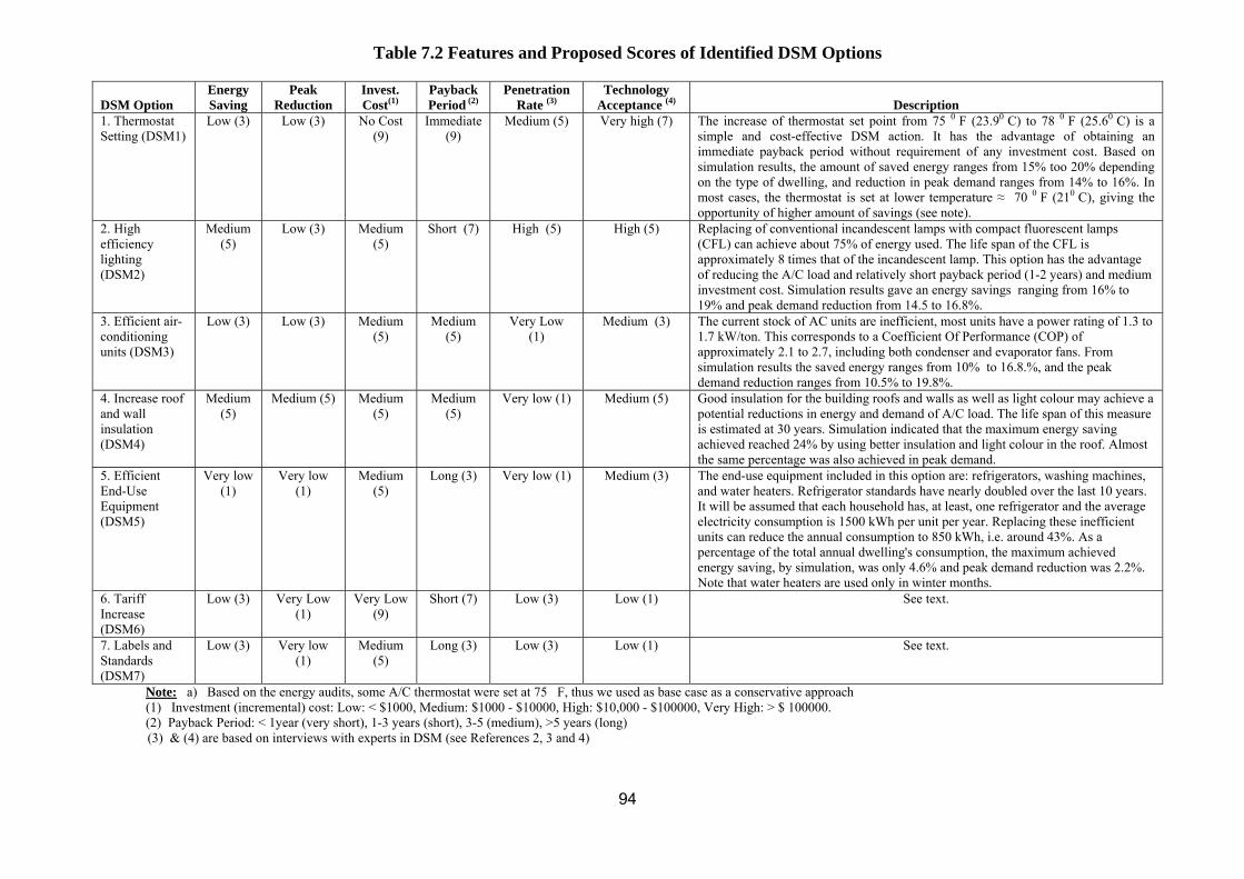
94

Table 7.2 Features and Proposed Scores of Identified DSM Options

DSM Option

Energy Saving

Peak Reduction

Invest. Cost(1)

Payback Period (2)

Penetration Rate (3)

Technology Acceptance (4)

Description

1. Thermostat Setting (DSM1)

Low (3) Low (3) No Cost (9)

Immediate (9)

Medium (5) Very high (7) The increase of thermostat set point from 75 0 F (23.90 C) to 78 0 F (25.60 C) is a simple and cost-effective DSM action. It has the advantage of obtaining an immediate payback period without requirement of any investment cost. Based on simulation results, the amount of saved energy ranges from 15% too 20% depending on the type of dwelling, and reduction in peak demand ranges from 14% to 16%. In most cases, the thermostat is set at lower temperature ≈ 70 0 F (210 C), giving the opportunity of higher amount of savings (see note).

2. High efficiency lighting (DSM2)

Medium (5)

Low (3) Medium (5)

Short (7) High (5) High (5) Replacing of conventional incandescent lamps with compact fluorescent lamps (CFL) can achieve about 75% of energy used. The life span of the CFL is approximately 8 times that of the incandescent lamp. This option has the advantage of reducing the A/C load and relatively short payback period (1-2 years) and medium investment cost. Simulation results gave an energy savings ranging from 16% to 19% and peak demand reduction from 14.5 to 16.8%.

3. Efficient air-conditioning units (DSM3)

Low (3) Low (3) Medium (5)

Medium (5)

Very Low (1)

Medium (3) The current stock of AC units are inefficient, most units have a power rating of 1.3 to 1.7 kW/ton. This corresponds to a Coefficient Of Performance (COP) of approximately 2.1 to 2.7, including both condenser and evaporator fans. From simulation results the saved energy ranges from 10% to 16.8.%, and the peak demand reduction ranges from 10.5% to 19.8%.

4. Increase roof and wall insulation (DSM4)

Medium (5)

Medium (5) Medium (5)

Medium (5)

Very low (1) Medium (5) Good insulation for the building roofs and walls as well as light colour may achieve a potential reductions in energy and demand of A/C load. The life span of this measure is estimated at 30 years. Simulation indicated that the maximum energy saving achieved reached 24% by using better insulation and light colour in the roof. Almost the same percentage was also achieved in peak demand.

5. Efficient End-Use Equipment (DSM5)

Very low (1)

Very low (1)

Medium (5)

Long (3) Very low (1) Medium (3) The end-use equipment included in this option are: refrigerators, washing machines, and water heaters. Refrigerator standards have nearly doubled over the last 10 years. It will be assumed that each household has, at least, one refrigerator and the average electricity consumption is 1500 kWh per unit per year. Replacing these inefficient units can reduce the annual consumption to 850 kWh, i.e. around 43%. As a percentage of the total annual dwelling's consumption, the maximum achieved energy saving, by simulation, was only 4.6% and peak demand reduction was 2.2%. Note that water heaters are used only in winter months.

6. Tariff Increase (DSM6)

Low (3) Very Low (1)

Very Low (9)

Short (7) Low (3) Low (1) See text.

7. Labels and Standards (DSM7)

Low (3) Very low (1)

Medium (5)

Long (3) Low (3) Low (1) See text.

Note: a) Based on the energy audits, some A/C thermostat were set at 75 F, thus we used as base case as a conservative approach (1) Investment (incremental) cost: Low: < $1000, Medium: $1000 - $10000, High: $10,000 - $100000, Very High: > $ 100000. (2) Payback Period: < 1year (very short), 1-3 years (short), 3-5 (medium), >5 years (long)

(3) & (4) are based on interviews with experts in DSM (see References 2, 3 and 4)

7.4 Example of AHP Calculations

The AHP procedure will be demonstrated in this example for illustration

purposes. The basic steps developed by Saaty38,39are followed in this example for the

selection of the best DSM option. Referring to Table 7.2 and the hierarchy of the

problem shown in Figure 7.2, the following can be done manually or automatically by

the AHP software, "Expert Choice"40.

7.4.1 Expert Choice:41,42

With Expert Choice, we define our goals, identify the criteria and alternatives,

and evaluate key trade-offs in a straight forward process. Expert Choice assists in

building a model for our decision and leads us in judging, via pair-wise comparisons,

the relative importance of the variables (DSM options). Expert Choice then synthesizes

our judgments to arrive at a conclusion and allows us to examine how changing the

weighting of our criteria affects our outcome.

As we create our decision model, we have to make certain assumptions (usually

based on previous experience) about the relative importance or value of various criteria

and alternatives (see Table 7.2). But what if we are not sure those assumptions are

correct … or we recognize that they are subject to factors that may change over time?

Expert Choice's five sensitivity Graphs will enable us to take some of the uncertainty

out of our decision making by quickly and easily testing the results using "what if"

scenarios. When we change the variables, Expert Choice promptly shows us the effect

on the outcome.

A full range of reports – either printed in hard copy or pasted into other

Windows applications – can be customized to individual needs for presenting results or

documenting the decision making process. Reports may include the entire decision

hierarchy in sideways or tree view, specific segments of the hierarchy, details of the

synthesis process, or sensitivity analysis.

The steps used in our AHP example are as follows:

1. Constructing a set of pair-wise comparison matrices (size 7 x 7) to indicate the

preferences or priority for DSM alternative in terms of how it contributes to each

criterion as shown in Table 7.3(a).

95

2. Synthesizing the pair-wise comparison matrix as shown in Table 7.3 (c).

Synthesizing is carried out by dividing each element of the matrix by its column

total. For example the value 0.130 in Table 7.3 (c) is obtained by dividing 1.0

(from Table 7.3 (b) by 7.667, the sum of the column items in Table 7.3 (b) (1 +

1.667 + 1 + 1.667 + 0.333 + 1 + 1). The priority vector shown in Table 7.3 (c)

can be obtained by finding the raw averages. For example, the priority of DSM1

with respect to the criterion "Saved Energy" in Table 7.3 (c) is calculated by

dividing the sum of the rows (0.13 + 0.13 + 0.083 + 0.13 + 0.13 + 0.13 + 0.13)

by the number of DSM options (columns), i.e., 7, in order to obtain the value

0.124. The priority vector for "Saved Energy", indicated in Table 7.3 (c) is given

below for all DSM.

0.124 0.219 0.131 0.219 0.044 0.131 0.131

3. Calculating the consistency ratio, by using the eigenvalue as follows:

1,000 0,600 0,600 0,600 1,667 1,000 1,667 1,000 1,000 0,600 1,000 0,600 0,124 1,667 + 0,219 1,000 + 0,131 1,667 + 0,219 1,000 + 0,333 0,200 0,333 0,200 1,000 0,600 1,000 0,600 1,000 0,600 1,000 0,600

3,000 1,000 1,000 0.860 5,000 1,667 1,667 1.521 3,000 1,000 1,000 0.912 0,044 5,000 + 0,131 1,667 + 0,131 1,667 = 1.521 1,000 0,333 0,333 0.304 3,000 1,000 1,000 0.912

3,000 1,000 1,000 0.912

(Weighted sum matrix)

96

Dividing all the elements of the weighted sum matrices by their respective priority

vector elements, we obtain:

0.86/0.124 = 6.940, 1.521/0.219 = 6.950, 0.912/0.131 = 6.960, 1.521/0.219 = 6.950

0.304/0.044 = 6.910, 0.912/0.131 = 6.960, 0.912/0.131 = 6.96

We then compute the average of these values to get the eigenvalue λmax (6.94 + 6.95 + 6.96 + 6.95 + 6.91 + 6.96 + 6.96) λmax = = 6.95 7 We now find the consistency index, CI, as follows: Consistency Index CI = (λ max-n)/(n-1) = -0,010 Where N = 7

According to Saaty: Assume the random consistency for the size of matrix = 7 RI = 1.32

Consistency Ratio CR = CI/RI -0,0073 < 0.1

As the value of CR is less than 0.1, the judgements are acceptable. Similarly, the

pair-wise comparisons matrices and priority vectors for the remaining criteria can be

evaluated as shown in Tables 7.4-7.8 respectively.

97

Figure 7.2 – Hierarchy Structure of DSM Options

Goal: Criteria: SE PLR IC PBP PR TA DSM Options: DSM1 DSM1 DSM1 DSM1 DSM1 DSM1 DSM2 DSM2 DSM2 DSM2 DSM2 DSM2 DSM3 DSM4 DSM5 DSM6 DSM7 DSM7 DSM7 DSM7 DSM7 DSM7 SE = Saved Energy PLR = Peak Load Reduction IC = Investment Cost PBP = Payback Period PR = Penetration Rate TA = Technology Acceptance

Table 7.3 (a) - Pair wise Comparison for "Saved Energy"

Saved Energy DSM1 DSM2 DSM3 DSM4 DSM5 DSM6 DSM7

DSM1 1 (3/3) (3/5) (3/5) (3/5) (3/1) (3/3) (3/3) DSM2 (5/3) 1 (5/5) (5/3) (5/5) (5/1) (5/3) (5/3) DSM3 (3/3) (3/5) 1 (3/3) (3/5) (3/1) (3/3) (3/3) DSM4 (5/3) (5/5) (5/3) 1 (5/5) (5/1) (5/3) (5/3) DSM5 (1/3) (1/5) (1/3) (1/5) 1 (1/1) (1/3) (1/3) DSM6 (3/3) (3/5) (3/3) (3/5) (3/1) 1 (3/3) (3/3)

Selecting the best DSM Option

.

.

.

.

.

.

.

.

.

.

.

.

.

.

.

DSM7 (3/3) (3/5) (3/3) (3/5) (3/1) (3/3) 1 (3/3)

98

Table 7.3 (b) - Pair wise Comparison for "Saved Energy" (With Column Totals)

Saved Energy DSM1 DSM2 DSM3 DSM4 DSM5 DSM6 DSM7

DSM1 1,000 0,600 0,600 0,600 3,000 1,000 1,000 DSM2 1,667 1,000 1,667 1,000 5,000 1,667 1,667 DSM3 1,000 0,600 1,000 0,600 3,000 1,000 1,000 DSM4 1,667 1,000 1,667 1,000 5,000 1,667 1,667 DSM5 0,333 0,200 0,333 0,200 1,000 0,333 0,333 DSM6 1,000 0,600 1,000 0,600 3,000 1,000 1,000 DSM7 1,000 0,600 1,000 0,600 3,000 1,000 1,000 SUM 7,667 4,600 7,267 4,600 23,000 7,667 7,667

Table 7.3 (c) - Synthesized Matrix for "Saved Energy"

DSM1 DSM2 DSM3 DSM4 DSM5 DSM6 DSM7 Priority Vector

Saved Energy DSM1 0,130 0,130 0,083 0,130 0,130 0,130 0,130 0,124 DSM2 0,217 0,217 0,229 0,217 0,217 0,217 0,217 0,219 DSM3 0,130 0,130 0,138 0,130 0,130 0,130 0,130 0,131 DSM4 0,217 0,217 0,229 0,217 0,217 0,217 0,217 0,219 DSM5 0,043 0,043 0,046 0,043 0,043 0,043 0,043 0,044 DSM6 0,130 0,130 0,138 0,130 0,130 0,130 0,130 0,131 DSM7 0,130 0,130 0,138 0,130 0,130 0,130 0,130 0,131 SUM 1,000 1,000 1,000 1,000 1,000 1,000 1,000 1,000

Table 7.4 - Pair wise Comparison for "Peak Load Reduction"

Peak Load Reduction DSM1 DSM2 DSM3 DSM4 DSM5 DSM6 DSM7 Priority

Vector DSM1 1 (3/3) (3/3) (3/3) (3/5) (3/1) (3/1) (3/1) 0,179 DSM2 (3/3) 1(3/3) (3/3) (3/5) (3/1) (3/1) (3/1) 0,179 DSM3 (3/3) (3/3) 1 (3/3) (3/5) (3/1) (3/1) (3/1) 0,197 DSM4 (5/3) (5/3) (5/3) 1 (5/5) (5/1) (5/1) (5/1) 0,267 DSM5 (1/3) (1/3) (1/3) (1/5) 1 (1/1) (1/1) (1/1) 0,060 DSM6 (1/3) (1/3) (1/3) (1/5) (1/1) 1(1/1) (1/1) 0,060 DSM7 (1/3) (1/3) (1/3) (1/5) (1/1) (1/1) 1(1/1) 0,060

99

Table 7.5 - Pair wise Comparison for "Investment Cost" Investment

Cost DSM1 DSM2 DSM3 DSM4 DSM5 DSM6 DSM7 Priority Vector

DSM1 1 (9/5) (9/5) (9/5) (9/5) (9/9) (9/5) 0,209 DSM2 (5/9) 1 (5/5) (5/5) (5/5) (5/9) (5/5) 0,116 DSM3 (5/9) (5/5) 1 (5/5) (5/5) (5/9) (5/5) 0,116 DSM4 (5/9) (5/5) (5/5) 1 (5/5) (5/9) (5/5) 0,116 DSM5 (5/9) 1 (5/5) (5/5) 1 (5/9) (5/5) 0,116 DSM6 (9/9) (9/5) (9/5) (9/5) (9/5) 1 (9/5) 0,209 DSM7 (5/9) (5/5) (5/5) (5/5) (5/5) (5/9) 1 0,116

Table 7.6 - Pair wise Comparison for "Payback Period" Investment

Cost DSM1 DSM2 DSM3 DSM4 DSM5 DSM6 DSM7 Priority Vector

DSM1 1 (9/7) (9/5) (9/5) (9/3) (9/7) (9/3) 0.231 DSM2 (7/9) 1 (7/5) (7/5) (7/3) (7/7) (7/3) 0.180 DSM3 (5/9) (5/7) 1 (5/5) (5/3) (5/7) (5/3) 0.128 DSM4 (5/9) (5/7) (5/5) 1 (5/3) (5/7) (5/3) 0.128 DSM5 (3/9) (3/7) (3/5) (3/5) 1 (3/7) (3/3) 0,077 DSM6 (7/9) (7/7) (7/5) (7/5) (7/3) 1 (7/3) 0,180 DSM7 (3/9) (3/7) (3/5) (3/5) (3/3) (3/7) 1 0,077

Table 7.7 - Pair wise Comparison for "Penetration Rate"

Penetration Rate DSM1 DSM2 DSM3 DSM4 DSM5 DSM6 DSM7 Priority

Vector DSM1 1 (5/5) (5/1) (5/1) (5/1) (5/3) (5/1) 0,294 DSM2 (5/5) 1 (5/1) (5/1) (5/1) (5/3) (5/1) 0,294 DSM3 (1/5) (1/5) 1 (1/1) (1/1) (1/3) (1/1) 0,059 DSM4 (1/5) (1/5) (1/1) 1 (1/1) (1/3) (1/1) 0,059 DSM5 (1/5) (1/5) (1/1) (1/1) 1 (1/3) (1/1) 0,059 DSM6 (3/5) (3/5) (3/1) (3/1) (3/1) 1 (3/1) 0,176 DSM7 (1/5) (1/5) (1/1) (1/1) (1/1) (1/3) 1 0,059

100

Table 7.8 - Pair wise Comparison for "Technology Acceptance"

Technical Acceptance DSM1 DSM2 DSM3 DSM4 DSM5 DSM6 DSM7 Priority

Vector DSM1 1 (7/5) (7/3) (7/5) (7/3) (7/1) (7/1) 0,280 DSM2 (5/7) 1 (5/3) (5/5) (5/3) (5/1) (5/1) 0,200 DSM3 (3/7) (3/5) 1 (3/5) (3/3) (3/1) (3/1) 0,120 DSM4 (5/7) (5/5) (5/3) 1 (5/3) (5/1) (5/1) 0,200 DSM5 (3/7) (3/5) (3/3) (3/5) 1 (3/1) (3/1) 0,120 DSM6 (1/7) (1/5) (1/3) (1/5) (1/3) 1 (1/1) 0,040 DSM7 (1/7) (1/5) (1/3) (1/5) (1/3) (1/1) 1 0,040

Now the pair-wise comparison is also used to set priorities for all six criteria in

terms of importance of each in contributing to the overall goal. Table 7.9 shows the

pair-wise comparison matrix and priority vector for the six criteria. Of course, the

highest priority, or extremely preferred, is given to the two criteria: saved Energy and

peak load reduction; followed by two equally strongly preferred: the investment cost

and the payback period; and with less importance come the last two criteria: Penetration

rate and technology acceptance, as shown in Table 7.9.

Table 7.9 - Pair-wise Comparison Matrix for the Six Criteria (With Column Totals)

SE PLR IC PBP PR TA Priority

Vector SE 1,000 1,000 1,286 1,286 1,800 3,000 0,225 PLR 1,000 1,000 1,286 1,286 1,800 3,000 0,225 IC 0,778 0,778 1,000 1,000 1,400 2,333 0,175 PBP 0,778 0,778 1,000 1,000 1,400 2,333 0,175 PR 0,556 0,556 0,714 0,714 1,000 1,667 0,125 TA 0,333 0,333 0,429 0,429 0,600 1,000 0,075 SUM 4,444 4,444 5,714 5,714 8,000 13,333 1,000

The last step is to combine the criterion priorities and the priorities of each DSM

alternative relative to each criterion in order to develop an overall priority ranking of the

101

DSM options which is termed as the priority matrix as illustrated in Table 7.10. The last

column of the Table represents the calculated overall priority vector.

Table 7.10 - Priority Matrix for DSM Options

SE (0,225) PLR (0,225) IC (0,175) PBP (0,175) PR (0,125) TA (0,075)

Overall Priority Vector

DSM1 0,124 0,179 0,209 0,231 0,294 0,280 0,203 DSM2 0,219 0,179 0,116 0,179 0,294 0,200 0,193 DSM3 0,131 0,197 0,116 0,128 0,059 0,120 0,133 DSM4 0,219 0,267 0,116 0,128 0,059 0,200 0,175 DSM5 0,044 0,060 0,116 0,077 0,059 0,120 0,073 DSM6 0,131 0,060 0,209 0,179 0,176 0,040 0,136 DSM7 0,131 0,060 0,116 0,077 0,059 0,040 0,087

It is clear from Table 7.10, that DSM1– Increasing of thermostat set point – is

the best alternative for any future DSM strategy. Ranking all seven DSM options

according to their overall priorities is as follows:

DSM1 (20.3%), DSM2 (19.3%), DSM4 (17.5%), DSM6 (13.6%), DSM3 (13.3%),

DSM7 (8.7%) and DSM5 (7.3%). For more explanations and details of the example of

AHP calculations refer to Appendix 7.

7.4.2 Sensitivity Analysis

A sensitivity analysis could be applied to investigate how sensitive the rankings

of the alternatives are to changes in the importance of the criteria. Expert Choice offers

five modes of graphical sensitivity analysis:

• Performance

• Dynamic

• Gradient

• Two-dimensional

• Difference

102

We shall use the performance sensitivity analysis to examine the sensitivity of

the alternatives with respect to lower-level criteria and how this would change in the

final decision.

The criteria are represented by vertical bars, and the alternatives are displayed as

horizontal line graphs. The intersection of the alternative line graphs with the vertical

criterion lines shows the priority of the alternative for the given criterion, as read from

the right axis. The criterion's priority is represented by the height of its bar as read from

the left axis. The overall priority of each alternative is represented on the OVERALL

line, as read from the left axis. The original priority case (base case) is illustrated in

Figure 7.4 (a).

Sensitivity analysis is then performed by modifying the weight of Saved Energy

(SE) that would be achieved by efficient lighting (DSM2) from "medium" (score 5) to

"high" (score 7). Keeping the criteria priorities constant, and making the necessary

calculations, it was found that the final ranking of alternatives has been changed as

shown in Figure 7.4 (b) and Table 7.11. The efficient lighting moved to the first priority

(20.7%) with slight difference from the thermostat setting (20.1%). Priority weights of

other alternatives are almost kept the same as in the base case.

Figure 7.4 (a) Performance Sensitivity AnalysisBasecase With Saved Energy Score “ " 5 DSM 2

21.9

17.9

11.6

18

29.4

2019.3

0

5

10

15

20

25

30

35

Saved E.Peak D.R.Inv. CostPB PeriodPen. LevelTech. Acc.Overall Criteria

%

0

5

10

15

20

25

%

Criteria Weights DSM1 DSM2 DSM3 DSM4 DSM5 DSM6 DSM7

103

Figure7.4 (b) Performance Sensitivity Analysis -Saved Energy for DSM 2 is Higher by 40% than Base Case

28.2

17.9

11.6

17.9

29.4

2.0

20.7

0.0

5.0

10.0

15.0

20.0

25.0

30.0

35.0

Saved E.Peak D.R.Inv. CostPB PeriodPen. LevelTech. Acc.Overall

Criteria

%

0

5

10

15

20

25

%

Criteria Weights DSM1 DSM2 DSM4 DSM5 DSM6 DSM7 DSM3

Table 7.11 - Priority Matrix for DSM Options

SE (0,225) PLR (0,225) IC (0,175) PBP (0,175) PR (0,125) TA (0,075)

Overall Priority Vector

DSM1 0.114 0.179 0.209 0.231 0.294 0.280 0.201 DSM2 0.282 0.179 0.116 0.179 0.294 0.200 0.207 DSM3 0.121 0.197 0.116 0.128 0.059 0.120 0.131 DSM4 0.201 0.267 0.116 0.128 0.059 0.200 0.171 DSM5 0.040 0.060 0.116 0.077 0.059 0.120 0.073 DSM6 0.121 0.060 0.209 0.179 0.176 0.040 0.134 DSM7 0.121 0.060 0.116 0.077 0.059 0.040 0.085

104

7.5 Summary

In this Chapter, the identified DSM options are analysed regarding their relative

importance, features and evaluation of their priority of implementation in any future

DSM programme in Kuwait. The evaluation process is complex due to the uncertainty

of penetration level and market trends in the residential sector. In such complicated

multi-criteria decision making process, it is required to select a reliable and intelligent

tool, that is capable of comparing each DSM option and evaluate them according to

multiple criteria measures.

The tool selected and applied in this Chapter for DSM evaluation and

prioritization is the Analytic Hierarch Process. An illustrative example has presented to

demonstrate the AHP process as applied to our case. The results of calculations have

shown that the first priority of DSM programme implementation is given to the first

DSM option "Increase of thermostat setting from 75 ˚ F to 78 ˚ F”. A sensitivity analysis

was performed to check the sensitivity of the final decisions to some changes in

judgements. By increasing the amount of saved energy achieved by DSM2 (efficient

lighting) by 40% (from score 5 to score 7), the priority of efficient lighting came to the

first place.

Chapter 7 also includes a brief description and emphasizing the importance of

the two recommended policy options: tariff increase and energy efficiency standards

and labelling.

105

Chapter 8

Potential Impacts of Priority DSM Options

8.1 Introduction

The results of energy audits and simulation, discussed earlier, have shown that

the identified DSM measures have a high potential of energy savings and peak demand

reductions on the end-use level. The question now is how to evaluate the aggregated

impacts of these measures on the residential sector level and hence on the national level

in an integrated DSM programme. In this Chapter, we estimate the integrated impact of

DSM options through a 10-year period of time, starting from 2010. This, of course,

assumes that the preparation of any DSM programme in Kuwait has to start during the

rest of this year and the beginning of 2010.

Based on the available data, it is important to answer several specific questions

for realistic estimation of the DSM impacts, for example:

• How to determine the baseline demand forecast, that is the anticipated trend in

energy consumption and power demand to the start of the year 2020 without

any DSM activities?

• How to determine the rate of penetration of the identified technological and

policy DSM options through out the sector?

• How to estimate the impacts on energy and power demands as a result of

implementing each DSM option, in all types of dwellings (villas, apartments

and traditional houses)?

• How to aggregate the simultaneous implementation of all DSM options, in an

integrated DSM programme?

With the lack of available and up-to-date statistical data and surveys on the

residential sector behaviour, we have to consider carefully several studies (relatively

old) that have been conducted by KISR43, and others.

106

8.2 Methodology

The first step for evaluating the impacts of DSM measures on energy

consumption and peak demand is to develop the baseline scenario of demand (for both

energy and peak load) forecast through the 10 year planning horizon (2010-2019). The

second step is to develop a forecast incorporating the current dwellings stock and the

projected new constructions through the period of forecast.

In the third step we estimate the annual programme impacts, i.e., the energy

savings in GWh and peak demand reductions in MW resulting from the implementation

of DSM options. Impacts are developed through a building block approach that

aggregates the impacts across end uses. These estimates have to take into consideration

the affecting parameters such as dwelling stock, penetration rate, number and type of

dwellings participating in the DSM programme and peak demand coincident factor.

The fourth step is to evaluate the economical and environmental impacts; this

includes calculations of the avoided utility costs, costs of saved energy, and the

associated reductions in GHG emissions (this will be presented in Chapter 9). Figure 8.1

illustrates the steps used in this methodology

Figure 8.1 – Steps of DSM Impacts Evaluation

Estimate the Environmental Impact of DSM Measures

Estimate the Economical Impacts of DSM Measures

Estimate the Aggregate Impacts DSM Measures

Determine Peak Demand Reductions in Each Stock of Dwelling Types

Determine Energy Savings in Each Stock of Dwelling Types

Determine Baseline Dwellings Forecast (2010-2020)

Determine Baseline Demand Forecast (2010-2020)

107

The formula used to estimate DSM impacts is very simple, and represented as: Achievable Potential of Energy Savings (ES) or Peak Demand Reductions

(PR) = Baseline Forecast x Penetration Rate x Unit Impacts ……… (1)

The baseline forecast is the amount of energy consumption and peak demand

that would have occurred in the absence of any DSM activities. The penetration rate is

the share of the market that elects to participate in the DSM programme. The unit

impact is the percent reduction in energy usage and peak demand that results from the

implementation of DSM option.

Achievable potential, as identified by ACEEE's research, is defined as the

amount of cost-effective energy efficiency improvement expected to be captured as the

result of specific policy or programme actions. This assumes that other efficiency

improvements attributable to normal consumer and market behaviour, as well as other

conservation policies programmes (if exist) are not neglected. This class of efficiency

potential is distinguished from technical and economic potential in three important

ways:

• First, as the term implies, achievable potential is defined in terms of what

realistically can be captured by explicit actions.

• Second, and following from the first point, achievable potential is time-

dependent. Achievable potential can be only realised by convincing consumers

to replace existing equipment and practices with new, more efficient equipment

and practices. It is often the case that consumers are most easily convinced to

adopt high efficiency alternatives when they must make equipment replacement

108

Decisions anyway. Therefore, what is considered achievable potential grows

over time as an increasing amount of existing equipment stock reaches the end

of its useful life (assuming diffusion increases with time and the old non-

efficient equipment are gradually phased out).

• Third, achievable potential intrinsically is a function of consumer behaviour.

The amount of potential one might expect is based on assumptions about what

consumers will do when faced with various policy and programme

interventions. Because estimates of achievable potential consider this difficult-

to-predict consumer behaviour, they are inherently more uncertain than

estimates of technical or economical potential.

Currently, according to our knowledge, in Kuwait neither DSM programmes,

nor any energy efficiency activities are now under implementation. Therefore we

assume that the recommended DSM measures, in our work, will be the only achievable

potential in the near future. It is very difficult to promote and implement any DSM

programme in Kuwait under the current low price of electricity. For this reason, we

assume that the achievable programme potential is most likely applicable with the

assumption that DSM options are implemented with high incremental cost incentives. A

good example of such incentive is to distribute CFLs to residential consumers with

lower price (e.g. half) than its actual price.

Below we discuss the elements of formula (1).

8.3 Baseline Demand Forecast

The prerequisite step to determine energy efficiency DSM potential impacts is to

establish the disaggregated baseline scenario of energy consumption and demand

forecasts that is to determine the trend of energy and demand forecasts without the

implementation of any DSM activity, and to establish the reference against which the

impacts of DSM measures can be assessed. These load forecasts are critical inputs for

the successful integration of DSM options. The forecast time horizon is 10 years,

starting from 2010 to 2019 inclusive.

Currently, there are no publicly available energy consumption forecasts that

include end-use sector (residential, industrial and commercial) breakdowns.

109

Based on the latest MEW Statistical Year Book of 2007, the development and

future estimates of the installed capacity, generated energy, peak load and load factor

are provided as shown in Table 8.1 for the period 2005 to 2010. The predicted values of

exported energy and final energy are shown in the Table. With these trends, the average

growth rates of the installed capacity, generated energy and peak load are 3.2%, 7.14%

and 7.3% respectively. As shown in the Table, the growth rates of exported energy and

final energy are the same and equal to 7.2%.

Back to the period 1995 – 2006, the statistical data of MEW indicates that the

growth of generated energy, peak load and exported energy is as shown in Table 8.2.

The average growth rate during this period was 6.6%, 5.95% and 6.9% respectively.

This means that, during recent years, and up to the end of 2010, the growth rate of

generated energy, exported energy and peak load are increasing which may create

shortage problems in the near future.

With reference to latest information published by MEW, the peak summer load

reached 8900 MW in 2006. The peak load profile occurred on 26 July 2006, illustrated

in Chapter 3, Figure 3.3, and is repeated below (Figure 8.2). The peak load and

extended from 14:30 to 15:30 at ambient temperature 49oC and relative humidity 6%.

We will assume that these growth rates are kept constant till the end of the

forecast period (2019 inclusive). Energy and power demand forecast (baseline scenario)

is shown in Appendix 8.1. The Appendix shows also the forecast of both exported

energy and final energy consumption. The exported energy is obtained form the

generated energy by extracting the energy consumed in the power plants (MEW –

2007), and the final energy consumption is obtained from the exported energy by

extracting the Transmission and Distribution (T & D) losses, which is estimated as

12%37. As shown in Appendix 8.1, the projected final energy consumption at the end of

2019 accounts for 89057 GWh and the projected peak demand may reach 20607 MW

that is exceeding the projected planned installed capacity by more than 3140 MW,

which will create a critical problem of shortage.

110

Table 8.1 Development of Energy and Power Demands from 2005 to 2010

Year 2005(*) 2006(*) 2007(**) 2008(**) 2009(**) 2010(**)Growth

Rate (2005-2010)

Installed Available Capacity (MW) 10189 10229 10655 11082 11736 11914 3.2%

Generated Energy (GWh) 43734 47605 48761 53476 58011 61660 7.11%

Exported Energy (GWh) 37906 41750 42422 46524 50470 53644 7.2%

Final Energy ((GWh) 33357 36582 37331 40941 44413 47207 7.2%

Peak Load (MW) 8400 8900 9070 10000 10680 11950 7.3% Annual Load Factor (%) 59,4 61,1 61,4 61,0 62,0 58,9 -0,13%

Source: MEW, Statistical Year Book, 2007 (*) Actual values (**) Values estimated by MEW

Table 8.2 Development of Generated Energy and Peak Load (1995 – 2006)

Year Generated Energy (GWh)

G. Rate

(%)

Peak Load (MW)

G. Rate

(%)

Exported Energy (GWh)

G. Rate

(%)

1995 23724 4730 20266 1996 25475 7.4 5200 9.9 21735 7.3 1997 26724 4.9 5360 3.1 22860 5.2 1998 29984 12.2 5800 8.2 25753 12.7 1999 31576 5.3 6160 6.2 26962 4.8 2000 32323 2.4 6450 4.7 27463 1.9 2001 34299 6.1 6750 4.7 29273 6.6 2002 36362 6.0 7250 7.4 31053 6.1 2003 38577 6.1 7480 3.2 33086 6.5 2004 41257 6.9 7750 3.6 35632 7.7 2005 43734 6.0 8400 8.4 37906 6.4 2006 47605 8.9 8900 6.0 41570 10.1

Average 6.6 5.95 6.9 (*) Equal to generated energy minus energy consumed by power plants.

111

Figure 8.2 - The Peak Load Profile "26 July, 2006"

6000

6500

7000

7500

8000

8500

9000

9500

0:00 2:00 4:00 6:00 8:00 10:00 12:00 14:00 16:00 18:00 20:00 22:00 0:00Time/Hrs

MW

8900 MW

8.3.1 Demand Forecast for Residential Sector

Unfortunately, recent data for the distribution of energy consumption by sector

is not available. Based on a study published by the World Bank in 1993, the

consumption of residential sector in 1989 was estimated at 63% of total consumption.

Industrial sector had a share of 20%, followed by the government with 10% and

commercial sector with 8%. Later, in 2002, articles published through KISR (Aasem,

and others, DBET) estimated the distribution of electricity consumption by sector as

illustrated in Table 8.3.

Between 1970 and 2001, the share of residential consumption had been

increased from 55% to 65% due to improved housing and higher per capita income,

which resulted in increased usage of central air conditioning and other appliances. It can

reasonably be assumed that residential consumption has continued to rise over the past

decade, as a consequence of further improved housing and higher space.

112

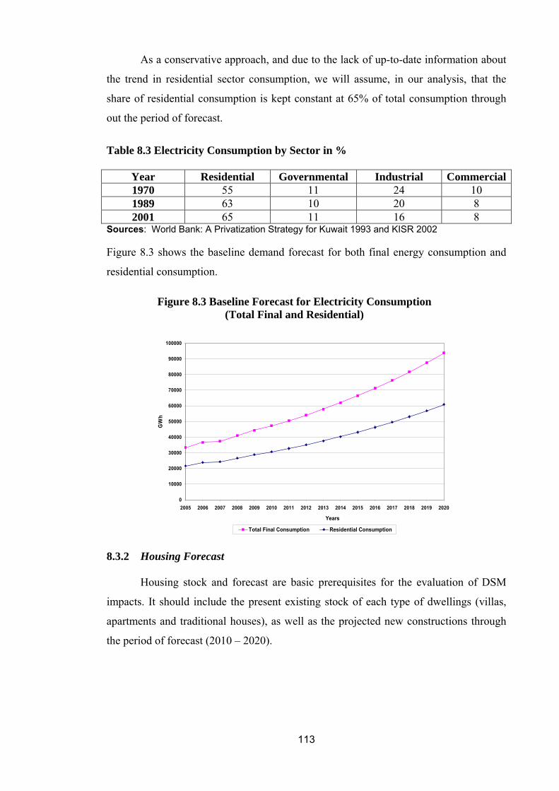
As a conservative approach, and due to the lack of up-to-date information about

the trend in residential sector consumption, we will assume, in our analysis, that the

share of residential consumption is kept constant at 65% of total consumption through

out the period of forecast.

Table 8.3 Electricity Consumption by Sector in %

Year Residential Governmental Industrial Commercial1970 55 11 24 10 1989 63 10 20 8 2001 65 11 16 8

Sources: World Bank: A Privatization Strategy for Kuwait 1993 and KISR 2002 Figure 8.3 shows the baseline demand forecast for both final energy consumption and

residential consumption.

Figure 8.3 Baseline Forecast for Electricity Consumption (Total Final and Residential)

0

10000

20000

30000

40000

50000

60000

70000

80000

90000

100000

2005 2006 2007 2008 2009 2010 2011 2012 2013 2014 2015 2016 2017 2018 2019 2020

Years

GW

h

Total Final Consumption Residential Consumption

8.3.2 Housing Forecast

Housing stock and forecast are basic prerequisites for the evaluation of DSM

impacts. It should include the present existing stock of each type of dwellings (villas,

apartments and traditional houses), as well as the projected new constructions through

the period of forecast (2010 – 2020).

113

With reference to the Annual Statistical Abstract of 2007, published by the

Central Statistical Office of Kuwait, the results of the three buildings censuses

performed in 1985, 1995 and 2005 are summarized in Table 8.4. The number of private

buildings has been increased from 102,510 in 1985 to 119,856 in 1995 to 165,029 in

2005, with an annual growth rate approximately 3.1%. The total number of dwellings

estimated through the three censuses is: 213,591 in 1985, 234,153 in 1995 and 303,045

in 2005. The classification of these dwellings is available only in 1985 census as

follows: 40,689 villas, 110,252 apartments, 33,106 traditional houses and 6,773 others.

Some efforts were made during the 90s for estimating the number of each residential

type. Taking into consideration these estimates and the available number of buildings in

2005, the approximate dwellings stock could be estimated as:

• 104650 Villas (35%)

• 122666 Apartments (40%)

• 36500 Traditional houses (12%), and

• 40229 Other (13%)

Other dwellings are mostly low-income dwellings, and will be excluded from

the forecast.

According to the Annual Statistical Abstract of Kuwait, the number of new

construction permits in 2006 and 2007 were 9957 and 11169 respectively, representing

about 6% and 6.4% of total residential buildings. On the other hand, the rate of new

dwellings construction (Villas, traditional houses and apartments), announced by the

Public Authority for Housing Welfare (PAHW), is approximately 3% per year.

Interviews with technical staff in the MOP indicated that approximately, the same

percentage is added every year by dwellings construction through private companies.

Therefore, the total additions of dwellings every year could be assumed 6% of the

existing stock.

Due to the unavailability of data on the exact numbers of future dwellings

construction classified by type, we will assume that the number shared by each dwelling

type is kept constant all-over the forecast period. This assumption is more conservative

with respect to DSM impacts, since the trend in Kuwait is to own/live in villas

(associated with higher consumption) than traditional houses and apartments.

Also, it was assumed in the Analysis that the demolition rate is negligible.

114

Table 8.4 – The Development of Private Buildings Stock

Census 1985

Type of Building Villa % Apartment % Tr. House % Other % Total

No. of Buildings 53839 52,5% 9959 9,7% 33670 32,8% 5042 4,9% 102510

Households 42323 19,1% 112448 50,7% 36358 16,4% 30642 13,8% 221771 Census 1995

Type of Building Villa % Apartment % Tr. House % Other % Total

No. of Buildings 61870 51,6% 9862 8,2% 30969 25,8% 17155 14,3% 119856 Households Na Na Na Na Census 2005

Type of Building Villa % Apartment % Tr. House % Other % Total

No. of Buildings 104650 63,4% 13579 8,2% 31000 18,8% 15800 9,6% 165029 Households Na Na Na Na 307285Source: Annual Statistical Abstract, Edition 44, 2007, Kuwait. 8.4 Penetration Rate of DSM Options

To estimate the achievable DSM potential, it is important to apply market

penetration rates (PR) to the technical potential estimates. In general, the penetration

rate of any DSM measure is uncertain and related to market conditions, end-use

technology, extend of cost sharing required by the consumer, the level of economic

awareness, customer acceptance and preference. However, one feasible method to deal

with uncertain circumstances is, for the experts in the field, to identify the most likely

scenarios based on their experience and available economic and technical data.

In our analysis the diffusion of DSM measures into the market and its adoption

by customers will be subject to the following assumption:

8.4.1 Market Transformation

While no single definition exists, market transformation generally refers to the

process by which collective action, policies and programmes effect a positive, lasting

change in the market for energy efficient technologies and services, such that these

115

Technologies and services are produced, recommended and purchased in increasing

quantity, (Suozzo and Nadel, 1996)44.

The essential role of market transformation programme, through DSM, is to

accelerate the adoption of energy efficient technologies and practices, resulting in

market transformation, or lasting change in the structure of the market, such adoption of

energy efficient technologies become normal or standard practice45.

To simulate the growth of energy efficiency DSM options market share over

time for the projected programme driven, we apply the simple logistic equation

represented by:46,47

k

Yt = ……………………………… (2) 1 + e

-b (t – tm )

where, Yt is the market penetration in year t; k is the maximum market

penetration, or saturation level; b is the penetration or diffusion rate; and tm is the time

required to reach 50% of the saturation level and is the inflection point in the logistic

curve.

Equation 2 produces the familiar S-shaped curve. The penetration rate b

specifies the "width" or "steepness" of the curve (e.g., b=0.19 means approximately

19% growth per time fraction). The logistic model is symmetric around the midpoint tm .

The parameter k, as discussed, is the asymptotic limit that the growth curve approaches,

i.e., market niche saturation.

In our analysis, we assume that the DSM technologies will compete with the

existing technologies according to the logistic formulation represented by Equation 2.

For example, in case of high efficiency lighting (DSM2), the CFL or LED lamps will

compete with the conventional incandescent lamps, through the DSM programme.

To implement this approach for appropriate adoption of DSM measures, it is

required to estimate suitable values of penetration rate taking into consideration market

conditions in Kuwait and expected barriers. Low penetration rates (less than 5%) are

116

Expected particularly in the early stages of any DSM programme, even with full support

from the government.

For example, the experience of the European Union in high efficiency lighting,

mainly the penetration of CFL, has shown that the penetration of CFL to the market is

on average less than 5% and in the households that owned CFLs is a bit above 10%

(based on 1995 data)48.

Given that the diffusion function employed is not directly linked to measure or

programme economies, we exercise judgment in selection parameter values that reflect

market condition and energy efficiency trends in one hand, and new DSM programme

intervention that would yield achievable potential on the other.

Figure 8.4 illustrates an example of S-curve representing the rate of adoption of

four DSM options. For the existing dwellings, the values of penetration rate "b" are

assumed as follows:

a) For DSM1 and DSM2 (see note) we assume that 80% saturation represents

full adoption of the two options by the year 2030. The other 20% are not

willing to participate.

We assume also that by the year 2020 only 50% of the fully adopted

residential consumers have implemented the two options. The promotion and

implementation of DSM1 depend mainly on the effectiveness of program

publicity. No hardware is required for this option; it is only required to

convince the consumer to increase thermostat setting from 75˚ F or less, to

78˚ F determined by ASHRAE as a comfortable level.

For DSM2, it was assumed that 80% of the installed conventional

incandescent lamps would be replaced to CFL, as indicated by simulation

process. This technology has been experienced with many countries, and has

been the target of a number of energy efficiency programs. Given the nature

of the market diffusion process, market share growth tends to be most rapid

relatively early in the market life of the technology if it offers compelling

market advantages and/or if it is heavily subsidized. Media will play an

important role to achieve higher levels of market penetration.

117

b) For DSM3 and DSM5, the use of efficient A/C equipment, and more

efficient end-use equipment (refrigerators, washing machines, water heaters,

etc.), we assume that only 20% of the saturation level could be adopted by

the year 2020. We assume also that the policy option DSM7, application of

Labels and Standards, is combined with DSM5. Both options are aiming to

the use of more efficient end-use equipment.

c) The penetration rate of the four DSM options, mentioned above, will be

assumed to be adopted by 20% of the new dwellings. The rest (80%) will be

added to the existing buildings that are subject to market behavior.

d) DSM4, the use of light colored roof and wall with high level of insulation: Is

assumed to be applied only for new buildings, with penetration rate fixed at

20%.

e) DSM6, tariff increase:

The impact of tariff increase on energy consumption is a difficult process

particularly in the condition of Kuwait, since the tariff has not been

increased in nominal terms for over thirty years, although the MEW has

considered tariff increases since the early 1980’s. In September 1999, a new

tariff proposal was submitted by the MEW. Under a 1995 law, the

government has to seek parliamentary approval when it comes to increasing

changes. The tariff proposal thus has to be approved by the Council of

Ministers and National Assembly. According to our knowledge, it is not yet

clear whether the approval would be granted. The expected effect of the

tariff increase on energy conservation cannot be quantified by MEW.

The proposal comprises a four-tier tariff for residential consumers 37

(private houses and apartment buildings) with a rising block structure (four

blocks each), and different tariffs for commercial, governmental and

industrial consumers and for beach cabins.

118

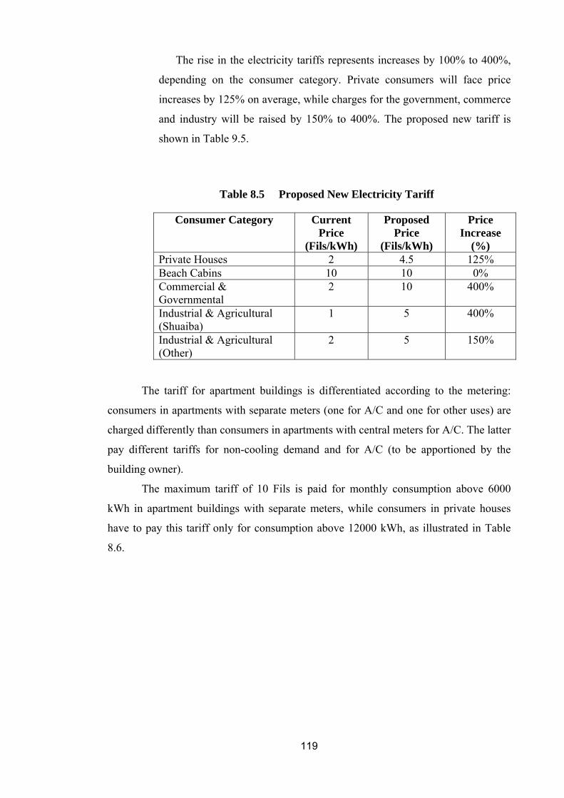
The rise in the electricity tariffs represents increases by 100% to 400%,

depending on the consumer category. Private consumers will face price

increases by 125% on average, while charges for the government, commerce

and industry will be raised by 150% to 400%. The proposed new tariff is

shown in Table 9.5.

Table 8.5 Proposed New Electricity Tariff

Consumer Category Current Price

(Fils/kWh)

Proposed Price

(Fils/kWh)

Price Increase

(%) Private Houses 2 4.5 125% Beach Cabins 10 10 0% Commercial & Governmental

2 10 400%

Industrial & Agricultural (Shuaiba)

1 5 400%

Industrial & Agricultural (Other)

2 5 150%

The tariff for apartment buildings is differentiated according to the metering:

consumers in apartments with separate meters (one for A/C and one for other uses) are

charged differently than consumers in apartments with central meters for A/C. The latter

pay different tariffs for non-cooling demand and for A/C (to be apportioned by the

building owner).

The maximum tariff of 10 Fils is paid for monthly consumption above 6000

kWh in apartment buildings with separate meters, while consumers in private houses

have to pay this tariff only for consumption above 12000 kWh, as illustrated in Table

8.6.

119

Table 8.6 Proposed New Electricity Tariffs for Residential Consumers

Apartment Building

Private House Separate

Meters Sep. Meters for Non-A/C

Central A/C

Meters

Current Price

(Fils/kWh)

Proposed Price

(Fils/kWh)

Price Increase

(%)

1-6000 1-1500 1-600 1-900 2 2 0% 6001-9000

1501-3000

601-1200 901-1700 2 4 100%

9001-12000

3001-6000

1201-2400 1701-3600

2 6 200%

Consumption Block from

kWh to kWh

>12000 >6000 >2400 >3600 2 10 400% Average 2 4.5(*) 125%

(*) Average based on the assumption that 70% of the consumers are in the lower two consumption brackets which pay an average price of 3 Fils/kWh, and that 30% pay an average of 8 Fils/kWh.

Since the tariff increase will multiply the present household expenses for

electricity, the proposal faces strong opposition from the consumers who have been

used to low electricity prices for more than a generation. The new tariff proposal,

however, takes into account equity considerations: In the lowest consumption bracket

the tariff remains unchanged. Assuming that a large share of the consumers falls into

these brackets, only the consumers with high consumption will be affected, who

typically are consumers with higher income. Thus it may be assumed that the tariff

increase will mainly affect the consumers who

(a) Can afford higher tariffs, and

(b) Have a high savings potential.

KISR Study on Tariff Effect

KISR study on tariff increase was conducted in 198749, to assess the impact of

alternative electricity tariffs with regard to electricity conservation, equity for

consumers and profitability for producers, government subsidy and macro-economic

effects. The study was only concerned with the energy savings impact and did not

estimate the effect on the peak load.

According to KISR study, the average residential consumption was 40,507 kWh

in 1984; the richest 10% of the households consumed about twice the average amount,

while the poorest consumed 75% of the average. Specific consumption more than

doubled between 1972/73 and 1984, and the average budget shares of electricity

120

decreased by 50% from 1.2% to 0.67%. Electricity expenses represented 2.1% of total

household budgets of the poorest 10% and 0.4% of the richest 10% of consumers.

In KISR study, a combination of time series and cross section data sets were

used to estimate demand functions for residential consumption. Cross section data was

used to estimate the income elasticity of demand, while the time series data served to

estimate the price elasticity of demand. Short term price elasticity was found to be in

the range of -0.09, and the medium run price elasticity (two to five years) in the order

of -0.30.

Table 8.7 shows the savings potential of tariff increase according to KISR study

conducted in 1987. Five tariff scenarios were tested, comprising three or four increasing

blocks between 0 and 7,500 kWh/ month with tariff between 2 and 28 Fils/kWh. In

addition two scenarios with a two-tier multi-tariff system (for two different housing

types) and rising block structure (over three blocks) were tested, and with 12 Fils/kWh

as the highest tariff, as proposed by MEW, and one with 28 Fils/kWh as the highest

tariff.

Table 8.7 Savings Potential of Tariff Increase According to KISR Study

Price Elasticity -0.09 Price Elasticity -0.30

Scenario Avg. new

Price (Fils/kWh)

Avg. Price

Increase

Avg. Consum.

Reduction

Computed Elasticity

Avg. new Price

(Fils/kWh)

Avg. Price

Increase

Avg. Consum.

Reduction

Computed Elasticity

A 5.6 180% -5.6% -0,031 5.66 183% -19% -0.104 B 5.76 188% -7.7% -0,041 5.76 188% -26% -0.138 C 6.10 205% -6.9% -0.034 6.11 206% -23% -0.112 D 7.3 265% -14.9% -0.056 7.30 265% -49% -0.185 E 7.5 275% -10.6% -0.039 7.50 275% -35.3% -0.128 F1 4.10 105% -5.1% -0.049 4.10 105% -17.5% -0.167 F2 2.95 48% -4.0% -0.084 2.95 48% -13.5% -0.284 G1 8.6 330% -11.0% -.033 8.60 330% -36.8% -0.112 G2 5.27 164% -9.8% -0.060 5.27 161% -33% -0.206

Source: KISR, “The Economic Impact of Changing the Structure of Electricity Pricing in Kuwait, Final Report, June 1987.

According to the results of the study, the reduction potential of tariff increase

was between 4% and 15% under the assumption of price elasticity of -0.09, and

between 14% and 49% under the assumption of a price elasticity of -0.30, depending on

the tariff scenario as shown in Table 9.7. The reported results, however, are not

consistent with the assumed price elasticity. An average reduction in consumption by

121

5.6%, following an average price increase by 180% (as in the tested scenario A)

representing price elasticity of (-5.6%/180% =) -0.031 instead of the explicitly assumed

elasticity of -0.09, as shown in the table above.

Thus, we may conclude that the short run prices elasticity were rather in the

range of -0.03 to -0.06, and the medium run elasticity in the range of -0.10 to -0.20.

These prices elasticity seem to be more realistic than the explicitly assumed price

elasticity of -0.09 and -0.30 respectively, for the following reasons:

• The actual impact of a tariff increase is determined by the general income level

and by the extent of the increase.

• Studies have shown that studies have a considerable impact on energy use in

countries where income is still low, but have a low impact on countries where

income is relatively high, because in these countries, like in Kuwait, expenses on

electricity have only a marginal share in the household budget. The price

elasticity of residential consumers in Kuwait is, therefore, expected to be rather

on the low side,

• Studies on prices elasticity generally refer to percentage increases of the

electricity tariff in the range of 1% to 50%, not to a doubling or tripling of the

tariff. When, as proposed in Kuwait, the tariff is increased by 100% to 400%,

electricity demand cannot be expected to react according to the standard price

elasticity: assuming a short run price elasticity of -0.10, a tariff increase by

400% would theoretically result in an immediate reduction of demand by 40%,

which is highly unrealistic, giving the technical restraints in short term energy

savings in Kuwait.

Based on the above background, we use in our analysis, two scenarios; one with

an average short term elasticity of -0,04 and a minimum medium term (five years) price

elasticity of -0.10. The price increase will be as proposed by MEW, i.e. with an average

price increase for residential consumers is in the range of 125%. Under the above

assumption, the energy consumption of the residential consumers will decrease as a

result of the price increases by 6% (125%*-0.04) and 15% (12.5% * -0.10),

respectively, over the period of forecast.

122

Peak demand reductions, associated with energy conservation, due to tariff

increase is hard to estimate. Since the average load factor is usually decreased due to the

reduction in energy consumption, we will assume that the peak load is reduced by, at

least, 1% and 2% for the short and medium term elasticity respectively. These minimum

impacts of tariff increase on peak demand are taken as a conservative approach. Table

8.8 summarizes the impact of tariff increase on energy consumption and peak load

considered in our calculations.

Table 8.8 Assumptions for the Potential Impact of Tariff Increase on Energy and Load

Reduction in Scenario Assumed Elasticity

Average Price Increase Energy Peak Load

Scenario 1 Short term : 0.04 125% 5% 1% Scenario 2 Medium term:

0.10 125% 12.5% 2%

On the other hand, we assume, in our analysis, that the government will enhance

adoption of recommended DSM options through positive incentives such as:

• Cost-sharing arrangements, in such a way that a considerable portion of the

initial cost is provided by MEW, so that the payback period for the residential

consumer is equal to or less than two years.

• The DSM programme cost is fully paid by the government.

• Information campaigns supported by the government.

Figure 8.4 Logistic S-Curve DSM Market Adoption

0,0% 10,0%

20,0%30,0%

40,0%50,0%60,0%

70,0%80,0%90,0%

100,0%

2010 2012 2014 2016 2018 2020 2022  2024 2026 2028 2030

DSM1 & DSM2 DSM3 & DSM5

DSM Market 

  Adoption

123

8.5 Unit Impact

The Unit Impact is the percent reduction in energy usage and peak demand that

results from the implementation of the DSM option. It will be assumed that all types of

dwellings adopted in the DSM programme are typical as that considered in the

simulation process. For a wide range of buildings, this assumption suffers from in-

accuracy. However, we assumed that the samples selected for energy audits and

simulation are most likely represent the majority of typical dwellings. Actually, energy

consumption in each type of dwellings is diversified. Accepting this diversity, our

assumption could reasonably represent the average patterns of energy consumption of

dwelling stock. Thus, the unit impacts of energy savings and peak demand reductions

used in our calculations will based on the results of simulation shown in Tables 6.3,

Chapter 6.

8.6 Cumulative DSM Impacts

The next step is to aggregate measure savings potential resulting from the

logical groups or bundles. This grouping exercise is important in fully integrated

resource planning because individual option savings are generally not large enough to

weigh against supply-side alternatives. The idea is to give the options enough critical

mass so that they can be selected by the resource planning model50.

Table 8.9 (A and B) displays the DSM impacts pertaining to the potential annual

energy reduction that could be achieved for each type of dwelling. Potential energy

savings from villas are more significant than that from apartments and traditional

houses. Table 8.9 (a) shows the results of calculations for the scenario of tariff price

elasticity of -0.04, while Table 8.9 (b) shows the scenario of tariff price elasticity of -

0.1. For the second scenario, the total potential of energy that could be saved by the end

of 2019 is approximately 4263 GWh, representing about 10.2% of total residential

consumption and about 4.96% of total end-use energy consumption. The accumulated

sum of the potential energy savings across the forecast horizon may reach 37229 GWh,

representing approximately 67% of the generated energy in the base year 2010 (see

Table 8.9 (b).

124

Table 8.9 (a) DSM Impacts by Type of Dwelling - Annual Energy Savings (GWh) (Scenario 1: Tariff Price Elasticity -0.04)

Year Villas Apartments Tr. Houses Total %

Residential % Final En.

Consumption 2.79% 2010 871.2 275.8 170.3 1317.3 4.79% 2.55% 2011 850.7 267.9 166.0 1284.7 4.46% 2.42% 2012 867.5 271.9 169.1 1308.6 4.33%

2013 895.7 279.5 174.5 1349.7 4.26% 2.33% 2.26% 2014 929.9 288.9 181.0 1399.8 4.22% 2.22% 2015 978.7 302.8 190.3 1471.9 4.23% 2.21% 2016 1048.2 323.0 203.7 1574.9 4.32% 2.22% 2017 1127.3 346.0 218.9 1692.1 4.43% 2.24% 2018 1218.9 372.6 236.5 1828.0 4.57% 2.25% 2019 1313.2 399.8 254.6 1967.5 4.69%

Total 10101.3 3128.4 1964.8 15194.5 Table 8.9 (b) DSM Impacts by Type of Dwelling - Annual Energy Savings (GWh) (Scenario 2: Tariff Price Elasticity -0.10)

Year Villas Apartments Tr. Houses Total %

Residential % Final En.

Consumption 6.65% 2010 2071.1 661.4 406.2 3138.7 11.41% 6.91% 2011 2300.0 731.4 450.7 3482.1 12.08% 6.52% 2012 2326.3 736.2 455.4 3517.9 11.64%

2013 2364.1 744.6 462.3 3571.0 11.28% 6.17% 5.86% 2014 2408.0 754.9 470.4 3633.2 10.95% 5.60% 2015 2466.6 769.6 481.3 3717.5 10.69% 5.39% 2016 2545.9 790.6 496.3 3832.8 10.52% 5.20% 2017 2634.9 814.4 513.1 3962.4 10.37% 5.03% 2018 2736.5 841.8 532.4 4110.7 10.27% 4.87% 2019 2840.9 869.8 552.1 4262.8 10.16%

Total 24934.2 7791.9 4867.3 37229.1

Table 8.10 (a) and Table 8.10 (b) display the DSM impacts pertaining to peak

summer demand reductions that have been developed through simulation and assumed

impacts of tariff increase with the first scenario of elasticity -0.04 and second scenario

with elasticity -0.1 respectively. By the year 2020 the aggregate sum of peak demand

125

reductions is estimated at 1245 MW and 1530 MW for the first and second scenarios

respectively, representing about 7.3% and 8.9% of the overall summer peak.

Table 8.10 (a) DSM Impacts by Type of Dwelling - Peak Demand Reductions (MW) - Scenario 1: Tariff Elasticity – 0.04

Year Villas Apartments Tr. Houses Total % Of Overall Peak Load

2010 113.3 190.1 34.6 338.0 3.1% 2011 109.6 183.8 33.7 327.2 2.9% 2012 120.4 201.9 37.4 359.6 3.0% 2013 136.9 229.7 42.8 409.5 3.2% 2014 157.9 265.0 49.8 472.7 3.6% 2015 187.4 314.5 59.7 561.6 4.0% 2016 230.0 385.9 73.9 689.8 4.7% 2017 281.5 472.3 91.3 845.1 5.5% 2018 344.5 578.0 112.7 1035.2 6.4% 2019 413.9 694.4 136.5 7.3% 1244.9 Total

Table 8.10 (b) DSM Impacts by Type of Dwelling - Peak Demand Reductions (MW) - Scenario 2: Tariff Elasticity – 0.10

Year Villas Apartments Tr. Houses Total % Of Overall Peak Load

2010 172.4 289.3 52.7 514.4 4.7% 2011 171.7 288.1 53.0 512.8 4.5% 2012 185.7 311.6 57.8 555.2 4.6% 2013 205.7 345.2 64.6 615.5 4.9% 2014 230.4 386.5 73.0 689.9 5.2% 2015 263.8 442.6 84.3 790.7 5.7% 2016 310.5 520.9 100.1 931.5 6.3% 2017 366.4 614.7 119.2 1100.3 7.1% 2018 434.0 728.2 142.4 1304.6 8.0% 2019 508.4 853.0 168.1 8.9% 1529.5 Total

Figure 8.5 shows the forecast of final energy consumption with and without

DSM impacts. The baseline consumption of residential sector is also shown in the

figure. Figure 8.6 shows the DSM impacts on summer peak demand.

126

Figure 8.5 DSM Impacts on Final Energy Consumption (GWh)

0

10000

20000

30000

40000

50000

60000

70000

80000

90000

100000

2010 2011 2012 2013 2014 2015 2016 2017 2018 2019

Years

GW

h

Baseline Final Energy Cons.

Final Energy Cons. with DSM (Sc.1)

Final Energy Consum. with DSM (Sc.2)

Figure 8.6 DSM Impacts on Peak Demand

0

2000

4000

6000

8000

10000

12000

14000

16000

18000

2010 2011 2012 2013 2014 2015 2016 2017 2018 2019

Years

MW

Basecase Peak Demand

Peak Demand Forecast (Sc. 1)

Peak Demand Forecast (Sc. 2)

Table 8.11, displays the accumulated energy saving across the period of forecast

(2010 – 2019), classified by DSM measure. From which it is clear that the impact of

tariff increase (DSM6) is highly significant and representing about 90% of total DSM

impacts.

127

Table 8.11 DSM Energy Saving Impacts by DSM Option

Energy Savings (GWh)

Dwelling DSM1 DSM2 DSM3 DSM4 +

DSM7 DSM5 DSM6 (*) Total

Total with 0.8

D.F. 857 906 390 66 107 20601 22927 22462 Villas

Apartments 256 271 111 4.4 30.2 6477 7149.6 7015 Tr. Houses 165 174 73.3 8.6 20.1 4031 4472 4384 Total 1278 1351 574.3 79 157.3 31109 34548.6 27639 D.F. = Diversity Factor (*) With Tariff Price Elasticity -0.10

Figure 8.7 shows the Load Duration Curve (LDC) for the base year 2010 and the

expected LDC for the year 2019 - inclusive with and without DSM impacts. The

reduction in peak demand in the terminal year 2020 is 1530 MW. The saved energy at

the start of 2020 is shown by the blue area of the curve.

Figure 8.7 the Impact of DSM Options on Load Duration Curve

Baseline LDC 2020 Curve

LDC 2020 With DSM

LDC 2010

0

2000

4000

6000

8000

10000

12000

14000

16000

18000

20000

0 372 1116 1848 2568 3300 4044 4776 5496 6228 6972 7716 8424 8760

Hours

MW

Baseline LDC LDC With DSM LDC 2010

128

8.7 Summary

Chapter 8 provides estimates for the potential energy savings and peak demand

reductions resulting by the implementation of identified DSM measures. A building

block approach was used to estimate the aggregate impacts of DSM options. Estimates

based on this approach resulted in several potential indicators related to energy savings

and peak demand reductions:

• By the end of forecast period (2010 – 2019 “inclusive”), the projected aggregate

savings in energy consumption may reach 4263 GWh representing about 10.2%

of the total residential consumption, and the peak demand reductions may reach

1530 MW representing 8.9% of the overall peak load.

• The total accumulated energy savings across the forecast period was estimated at

approximately 37229 GWh through the whole DSM programme.

• The tariff increase, or DSM6, has significant potential in reducing growth in

Kuwait energy consumption, where the achievable potential accounting for

about 90% of total DSM impacts, for a price elasticity -0.10.

The next step is to estimate the potential financial and environmental impacts associated

with the implementation of DSM measures. This will be discussed in Chapter 9.

129

Chapter 9

Economical and Environmental Impacts

9.1 Introduction

In Chapter 8 the potential achievable impacts of the identified priority DSM

options were estimated in the form of energy savings in GWh and peak demand

reductions in MW.

In this Chapter, the economical and environmental impacts of the identified

DSM measures are evaluated through the implementation of a DSM programme

executed from 2010 to 2020 and initiated by the MEW of Kuwait. A number of specific

questions are addressed in the present Chapter, including:

• What is the cost of saved energy (CSE) for each DSM option?

• What are the revenues achieved by saving energy / power?

• How the cost-effectiveness for each DSM option is evaluated?

• What is the amount of CO2 reductions that could be achieved by the

implementation of DSM options?

The Chapter includes the basic formulas used for calculations, economic

assumptions, the methodology used for calculations, as well as models of spread sheets

used for calculations.

9.2 Economic Benefits/ Cost Analysis

Economic screening, which follows the identification of DSM technologies and

the assessment of their technical potential, as presented in Chapter 8, is the main

determinant of a measure's acceptance or rejection. It entails an analysis of the costs and

benefits associated with each of the selected DSM measures. Benefits are typically

calculated from marginal costs of energy and capacity. Cost/benefit analysis can be

carried out in many degrees of detail.

Cost/benefit analysis of DSM measures has been discussed in many studies and

publications. DSM measures are evaluated in these studies either as self sustained

energy conservation technologies or as a part of Integrated Resource Planning (IRP)

(UNEP, 1997)51.

130

Most of these studies use a common approach involving screening the potential

DSM measures by comparing each measure's Cost of Saved Energy (CSE) and Cost of

Saved Capacity (CSC) with the avoided energy and capacity costs52. Measures for

which the CSE and CSC exceed the avoided energy and capacity costs are rejected

because any such DSM measures are more expensive than supply-side alternatives.

Measures for which at least one of these two values is less than the corresponding

avoided cost are retained to form the basis for a DSM programme. Programme design

specifies how some combination of measures will be marketed, delivered to customers,

tracked, and evaluated. The process of building up programmes around DSM measures

is outside the scope of this work.

In the next sections, we introduce briefly the basic definitions of avoided cost,

the CSE and the CSC. These definitions are given in details in Appendix 3 of Reference

1 (UNEP 1997).

9.2.1 Avoided Cost

From the perspective of resource economics, the value of DSM is measured by

the electricity supply costs that would be required without the DSM savings to

electricity use. These supply-side costs are collectively referred to as "avoided costs".

One key element of the avoided cost is the capital costs of electric generating plant.

Other elements of avoided cost include:

• Plant operation and maintenance (O & M) costs.

• Fuel costs.

• Transmission and distribution (T & D) costs.

In Kuwait, official up-to-date information from MEW about the avoided energy

and capacity costs are not available, however, several technical papers and studies

conducted by the staff of KISR considered the following cost estimates for their

analyses6,53,54

131

• Avoided Energy Cost:53 As mentioned in Chapter 3, the actual cost of producing each kWh has been

estimated in the range of 14 to 26 fils, while the residential consumer pays a flat rate of

2 fils/kWh (≈ US¢ 0,6). That is there is a subsidy of 12 to 24 fils/kWh.

In our analysis, the minimum avoided energy cost (14 fils/kWh) will be

considered.

• Avoided Capacity Cost:6,8,9,54 For the nation, the cost of power equipment, transmission and distribution, is

around KD 400/kW. On the other hand MEW charges the consumer for cable

connection KD 50 per kW. In our calculations, KD400/kW ((≈ US1200/kW) will be

assumed.

9.2.2 Cost of Saved Energy (CSE)

The CSE is defined as the annualized incremental cost of the DSM measure

relative to the cost of standard equipment, divided by the annual kilowatt-hour saving..

In other words, the CSE is the sum of net annualized capital costs of an

efficiency DSM measure and its net increase (or decrease) in operating costs, divided by

the annual energy savings:

ALCC CSE = ……………………(1) D Where, CSE = Cost of saved energy (e.g., $/kWh) ALCC = Modified annualized life cycle cost (e.g., $/year) of the

DSM measure: this cost should not include savings from reduced energy consumption,

D = Annual energy savings (e.g., kWh/year) The formula of the CSE can usually be simplified by assuming that the energy savings are a uniform annual series, in which case: (CRF . Cc + Cop) CSE = …………………………(2) D Where

132

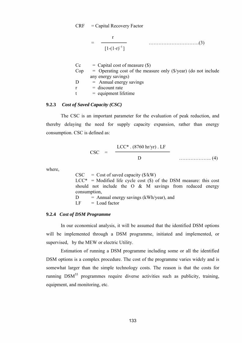
CRF = Capital Recovery Factor r = ………………………….(3) [1-(1-r)- t ]

Cc = Capital cost of measure ($) Cop = Operating cost of the measure only ($/year) (do not include

any energy savings) D = Annual energy savings r = discount rate

t = equipment lifetime 9.2.3 Cost of Saved Capacity (CSC)

The CSC is an important parameter for the evaluation of peak reduction, and

thereby delaying the need for supply capacity expansion, rather than energy

consumption. CSC is defined as:

LCC* . (8760 hr/yr) . LF CSC = D ……………….. (4) where, CSC = Cost of saved capacity ($/kW) LCC* = Modified life cycle cost ($) of the DSM measure: this cost

should not include the O & M savings from reduced energy consumption,

D = Annual energy savings (kWh/year), and LF = Load factor 9.2.4 Cost of DSM Programme

In our economical analysis, it will be assumed that the identified DSM options

will be implemented through a DSM programme, initiated and implemented, or

supervised, by the MEW or electric Utility.

Estimation of running a DSM programme including some or all the identified

DSM options is a complex procedure. The cost of the programme varies widely and is

somewhat larger than the simple technology costs. The reason is that the costs for

running DSM55 programmes require diverse activities such as publicity, training,

equipment, and monitoring, etc.

133

Most programmes report costs of saved energy of $0.02/kWh or less (Nadel et al

1990)56 . In USA, an ACEEE survey of state efficiency found reported lifecycle costs of

2.3 – 4.4 cents per kWh for seven states that reported these costs.

Generally, the programmes with high rates of free-riders (those who consume

more than their fair share of a public resource) involve measures that are highly cost-

effective and therefore have very low technology costs.

For a vigorous penetration of DSM options, financial incentives like initial

capital subsidies, low-interest credit schemes, accelerated depreciation, tax rebates, etc.

are essential for successful DSM programmes. Due to the extremely low electricity

tariff in Kuwait, we propose that a portion of the initial capital cost, for each DSM

option, is to be provided on a cost-sharing basis so that the contribution of utility

(MEW) is not less than 50% depending on the DSM measure implemented. In addition

to cost sharing, other indirect programme costs are necessary for publicity, generating

awareness, information campaign, utility staff salaries, conducting feasibility studies,

and costs for evaluating or monitoring programme results.

Total programme cost per kWh saved depends on the measure lifetime and the

discount rate used. It also depends on the estimated amount of saved energy on an

annual basis (Hirst, 1991)57, indicates that a utility DSM programme's performance

depends on two factors: Participation in the programme and the net savings of the

programme. The net savings of the programme is defined as:

Net programme savings = avoided supply costs – total programme costs ………. (5)

The total cost of saved energy consists of two components and can be expressed

as follows:

Programme CSE = (Ccap + Cind) . crf / D ……………………… (6) Where, CSE = Cost of saved energy ($ / kWh) Ccap = Capital cost of end-use technology Cind = Indirect costs of DSM programme crf = Capital recovery factor D = DSM programme annual kWh savings

134

Calculations of capital cost of end-use DSM measure (Ccap) and the indirect

cost of DSM programme (Cind) are based on the following main issues and

assumptions:

i) The indirect, or fixed, programme cost (Cind) consists usually from the

initial programme set up cost, programme costs for publicity, generating

awareness, conduction feasibility studies, training and monitoring and

evaluation of the programme. In our analysis, it will be assumed that the

indirect programme cost, for almost all options, is fixed at 2 fils/kWh

($0.006/kWh) of saved energy, i.e. the indirect programme cost for 2010 is

approximately 6.3 million KD (≈ $20 million), since the saved energy in this

year is estimated at 3139 GWh.

The assumption of such indirect programme cost is based on the following

issues:

• The cost of the programme per kWh represents only 14% of the

minimum avoided energy cost (2/14) and equal to electricity price

offered to residential consumers.

• Programme budget of about $20 million every year is quite

reasonable for any DSM pilot programme.

ii) The capital, or direct, cost (Ccap) of the programme depends on the type and

complexity of the DSM measure. It is comprised primarily of incremental

measure costs. Incremental measure costs are essentially the costs of

obtaining energy efficiency. In the case of an add-on device (say, roof

insulation, or shading), the incremental cost is simply the installation cost of

the measure itself. In the case of equipment that is available in various levels

of efficiency (e.g., a central air conditioner), the incremental cost is the

excess of the cost of the high efficiency unit over the cost of the base

(reference) unit.

It is important to emphasize that the higher the percentage of measure costs

paid by the programme, the higher the participants' benefit-cost ratios and,

consequently, the number of measures adoptions.

iii. Rebates, when applied, are structured either as fixed payments per unit

(e.g., $10 per electronic ballast) or as payments designed to lower the first

135

cost of a DSM measure to some predetermined level (e.g., to ensure a

payback period to the customer within three years).

B/C Model Development:

Calculation of the Benefit/Cost (B/C) ratio for each DSM option is carried out

using the following simple formula:

Benefits (CNPV)

B / C Ratio = ……………………..(7) Costs (CNPV) Where, CNPV is the cumulative net present value

Below, we discuss the main financial parameters of identified DSM options and

estimate the levelized costs for each option.

The range of discount rates used in energy efficiency studies vary, with most

analysis using a real discount rate of 4-8 percent to evaluate the cost-effectiveness of

energy efficiency policy. For example, ACEEE uses 5% while DOE employs a real

interest rate of 7%. Over the last few years, most nominal interest rates have been below

the real discount rate used by DOE.

In our calculations we assume a real discount rate of 4.5%.

i. Increase of Thermostat Setting (DSM1):

Increase of thermostat set-point from 23oC to 25oC saves, at least, 9% (average

simulated savings is 17%). This option costs nothing to implement, i.e. Ccap = 0; the

only costs to be spent is the indirect, or fixed, programme costs. We assume that

specific indirect programme cost is 2 fils/kWh (≈ $0.006/kWh) of saved energy. Based

on simulation results, the total amount of programme cost in the first year of forecast

(2010) is approximately KD 2528200 (≈ $ 7.6 million).

ii. High Efficiency Lighting (DSM2):

The majority of Kuwaiti houses use the conventional incandescent light bulbs.

Replacement of these bulbs to compact fluorescent lamps (CFL) is an attractive and

cost-effective DSM option. The average dwelling in Kuwait consumes roughly from

136

5000 to 8000 kWh per year on lighting, depending on the type of dwelling. By replacing

the existing incandescent lamps with CFL will save, at least, 70% of lighting electricity.

The lifetime of CFL is about 10000 hours (≈ 5 years), approximately 10 to 15 times

longer than incandescent bulbs. On annualized cost basis, a CFL may cost less than the

total cost of all the incandescent bulbs that have been replaced.

In our financial analysis, we focus only on two types of incandescent lamps to

be replaced to CFL, the 100 W and the 40 W (frequently used in chandeliers) bulbs. The

equivalent CFL lamps are 23 W and 7 W respectively. Table 9.1 shows the basic data of

lighting system based on energy audits and market trends.

Table 9.1 Lighting System Basic Data

Incandescent Lamps Average Number & Operation CFL Power (W)

Lifetime (Hours)

Cost ($)

Villa Apart-ment

Tr. House

Avg. Op. Hours/day

Power (W)

Lifetime (Hours)

Cost ($)

100 1000 0.5 28 14 30 6 23 10,000 5 40 1000 0.5 68 16 48 4 7 10,000 5

The average market price of CFL is assumed to be $5 and the percentage of

utility sharing is 50%. It is clear from Table 10.1 that, on annualized cost basis, a CFL

may cost less than the total cost of all incandescent bulbs that it is replacing.

Table 10.2 shows an example of programme cost components for the DSM

lighting option (DSM2). The example is applied to villas participating in the DSM

programme starting in 2010 and extended to the end of 2019. From the total resource

cost perspective, this DSM option is cost-effective giving a net benefit-to-cost (B/C)

ratio of 3. For the consumer, even with 50% cost sharing from the utility, the simple

payback period is about 3.4 years, which could be acceptable irrespective of very low

electricity price.

iii. High Efficiency Air Conditioning Units (DSM3):

The current stock of air conditioning (A/C) units is inefficient, most of the units

has energy efficiency ratio (EER) less than, or equal to 9. As previously analysed by

simulation process, we assume that the existing A/C units have been replaced by energy

efficient units of EER not less than 11. The incremental cost of efficient units with

respect to the existing units is assumed approximately 10 $/RT, therefore, the average

137

budget required to upgrade the existing 45 RT central air conditioning system in a villa,

for example, is around $450. The expected life span of the A/C unit is 15 years.

iv. High Quality Wall and Roof Insulation (DSM4)

Different insulating materials are used in Kuwaiti homes for walls and roofs.

Insulating the building roofs and walls with high quality 5 cm (2 inches) polystyrene

sheets, as well as light coloured surfaces, reduces energy use by, at least, 20% (average

simulation savings is 24%). The incremental cost of this measure is about US$500 per

dwelling. The life of the measure is estimated at 25 years.

138

Table 9.2 – Example of DSM Programme Costs for CFL Rebate Programme

Item Value A. CFL Rebate Programme – Cost Estimates Number of participating Villas (2010) 4290 Number of lamps / villa 28 (100 W)

68 (40 W) Annual savings /villa (kWh) 5658 Total annual energy savings (MWh) 1 24273 Total number of lamps adopted through programme (80%) 96096 (100W)

233376 (40W) Lifetime of CFL (years) 5 CFL market price $ 5 CFL rebate (%) 50 CFL final price to household / lamp $2.5 CFL cost to utility / lamp $2.5 B. DSM Programme: B1- Programme Fixed (Indirect) Cost (Publicity, advertising production, campaign, training, etc.) / kWh of saved energy

$0.006 (2 fils/kWh)

Total Programme fixed costs $145638 B2 – Programme Capital (Variable) Cost CFL cost to utility $823680 Total Utility Cost $969318 Utility real discount rate 4.5% Utility capital recovery factor 0.228 Equivalent annual utility programme cost 221005 Programme cost of saved energy $0.009/kWh

(≈ 3.0 fils/kWh) Net savings to Utility [ (12- 3) fils/kWh] 9 fils/kWh

($0.027/kWh) Benefit/Cost Ratio (B/C) 3.0 CFL Cost to Household ($) 2.5 x 96 x 0.8 = 192 Savings from replacing incandescent lamps ($) 76.8 Net Cost of replaced lamps ($) 115.2 Annual energy savings to Household ($) 2 34 Simple payback period for Household 3.4 years

1. Simulation results indicate higher saving (24273 MWh). 2. Electricity price is 2 fils / kWh ($0.006/kWh)

139

v. Energy Efficient End-Use Equipment (DSM5)

This option is assumed to be combined with DSM 7, the application of Labels

and Standards.

As a starting point for the promotion of Labels and Standards, it is common to

start with two or three kinds of end-use equipment, such as refrigerators, washing

machines and water heaters. We assume that the incremental cost required to Upgrade

these equipment is $150 per unit for villas and traditional houses and $100 per unit for

apartments. It will be assumed that 3 units are replaced for each villa and traditional

house, and two units for apartment. The lifetime of a refrigerator, washing machine and

water heater is assumed to be 10 years.

vi. Tariff Increase (DSM6)

The potential impact of tariff increase depends largely on DSM programme

design, tariff policy and information and awareness campaigns. Investment in this

option is assumed to be constant at a rate 2 fils ($0.006) per kWh of projected saved

energy. For example, the total programme cost allocated to promote tariff increase for

villas is 136.42 million US$ (Energy savings (22737 kWh) x $0.006), and the present

value of the programme cost on annual basis is 1724000 $/year.

9.2.5 Cost Effectiveness of DSM Programme58

A number of tests commonly used to assess a DSM programme's cost

effectiveness. Most of these tests are based on the perspectives of various stakeholders

involved in the DSM process. These tests include the following main types:

• The Utility Test (UT):

The UT measures the net costs of DSM as a resource option based on costs

incurred by the utility against the avoided costs of the supply.

• The Participant Test (PT):

The PT measures the quantifiable benefits and costs to the customer for a given

DSM measure. Due to very low electricity price, this test is difficult to be implemented

in Kuwait, since the payback period, from the customer perspective, will be very high.

140

• Total Resource Cost Test (TRC)59 :

The TRC test compares the avoided cost of supply with both the utility and

participant costs of a DSM measure. A benefit cost ratio of more than 1.0 indicates that,

for the particular group of economic actors, programme benefits outweigh costs, and the

programme can be considered cost-effective. In other words, a DSM measure with a

total cost of saved energy ($/kWh saved) less than current average electricity avoided

supply cost estimated by the Utility (MEW) as 14 fils/kWh ($0.042 / kWh) is

considered cost-effective.

The primary test that is used for screening DSM programmes is the Total

Resource Cost Test (TRC). This test assesses whether or not the programme improves

economic efficiency in the broad sense of the term. It compares the benefits of the

programmes to society with the costs to society of implementing the programme. The

benefits include the avoided cost of capacity and energy while the costs include the

equipment and administrative costs involved in executing the programme.

The administrative costs include staff time and other costs that are necessary to

design, implement, monitor and evaluate the program impacts. The test excludes any

transfer payments between members of the society. Thus, incentive payments by the

utility to recruit customers and taxes (of all kinds) that are paid by either the utility or

the customer are excluded from the calculation.

The application of these tests for anticipated DSM programme in Kuwait needs

careful attention due to the following reasons:

• These tests were developed in the U.S. context to assist the regulator in

determining the appropriateness and justification of for various utility DSM

programmes and may not be appropriate for other DSM programmes.

• While these tests may be considered as useful indicators for cost-effectiveness,

their use may be not sufficient to capture other important benefits, such as

building of public awareness, improved customer services, environmental

benefits, reduced fuel consumption, and other benefits commonly associated

with DSM programmes.

141

In the analysis the TRC test is used as to evaluate cost-effectiveness. Screening

worksheets are used to assess cost-effectiveness for all DSM options.

9.2.6 Economic Assumptions

Evaluation of cost-effectiveness and economic parameters are based on the

following assumptions:

• US$ is equivalent to 0.300 KD.

• The discount rate = 4.5%

• The life span of end-use equipment considered in the analysis is shown in Table

9.3

• For economic analysis, all values are presented in 2009 with USA dollars, with

costs and benefits after 2010 discounted, using the above mentioned discount

rate.

• The incremental installed cost of a DSM measure is its cost.

• Net economic benefits are considered over the lifetime of energy efficiency

DSM measures installed during 2010-2020.

Table 9.3 Residential Equipment Life Span

Appliance Average Life Span (years) Compact Fluorescent Lamps 5 Insulation/Building Envelop Improvement 25 Refrigerators & other end-use equipment 10 Air Conditioning Systems 15 Electric Hot Water Heaters 10-12

9.3 Economic Results

For each type of dwellings, a simple excel spread sheet model was developed for

use in calculating Benefit/Cost (B/C) ratio. For each DSM measure, functionality was

designed into the spread sheet to quantify benefits by multiplying the annual energy and

capacity savings values over their identified measure life, times the cumulative net

present value of a nationwide estimate of avoided energy and capacity costs over the

same measure life time period.

142

143

A summary of these results for all options and for each type of dwellings is

shown in Table 9.4. As shown in the table, the net savings for each DSM option,

classified by type of dwelling are estimated. The net benefits for all DSM options are

approximately:

• US$ 292 million for villas,

• US$ 79 million for apartments,

• US$ 47 million for traditional houses.

The corresponding B/C ratios are 12.5, 9.5 and 8.9 respectively. The total net

benefit that could be achieved by implementing all DSM options reaches US$ 417.7

million.

As shown in the Table, all DSM options are cost-effective with B/C ratio higher

than 1, except DSM4 (High quality roof and wall insulation) when applied to the

apartments, where it gives a negative value. This result for DSM4, under the proposed

scenario of investment, makes its inclusion in a DSM programme not warranted.

144

Table 9.4 Summary of Economic Impact Estimates by DSM Option (2010 – 2019)

Total Savings (1000$) Total Prog. Costs (1000$) NET Benefits (1000$) B/C Ratio (2)

DSM Option ID Villa Apartment TR.

House Villa Apartment TR. House Villa Apartment TR.

House Villa Apartment TR. House

Thermostat Resetting from 75 to 78 o F DSM1 133275 54376 27669 715 214 138 132561 54163 27532 185.4 253.7 200.0

Replacing Incandescent Bulbs to CFL DSM2 139138 50057 32367 943 3012 1545 138195 47045 30822 146.5 15.6 20.0

Upgrade A/C Equipment to Efficient Units with EER ≥ 11

DSM3 92413 31799 15928 2635 1083 688 89778 30716 15240 34.1 28.4 22.2

High Quality Wall and Roof Insulation DSM4 48833 26 682 980 159 177 47853 -133 505 48.8 -0.8 2.9

Use Energy Efficient End-Use Equipment (1) DSM5 15523 2573 1358 2399 1676 722 13124 896 636 5.5 0.5 0.9

Tariff Increase DSM6 158387 52902 32350 17183 5402 3362 141204 47500 28988 8.2 8.8 8.6

Total 315156 87299 52298 23393 8354 5267 291763 78945 47031 12.5 9.5 8.9

(1) Combined with DSM7 (Labels and Standards) (2) Cost-effective if B/C > 1.0

9.4 Environmental Impacts

Electricity generation results in the emission of pollutants, i.e. CO2, SO2, NO2

and fly ash. We shall focus on the emission of CO2, the main contributor in Greenhouse

Gas (GHG) emissions. Estimation of reduction in GHG emissions is becoming

increasingly important as climate change becomes a driver for many sustainable –

energy projects, including energy efficiency DSM projects.

The amount of GHG emissions decreased, or avoided, will depend on the DSM

energy efficiency measure used and the generation mix as well as type of fuel used in

power generating systems before and after the energy efficiency programme. In Kuwait,

power plants use both natural gas (NG) and liquid fuel. Specific data on fuel

consumption rates (gm/kWh) and power plants environmental aspects are not available.

However, the total type fuel and amount of energy used (in billion Btu) in each of the

power plants are available (see Table 9.5). Part of this energy is used for desalination,

thus the actual plant efficiency actually higher than that shown in Table 9.5. Based on

our estimates, the average specific energy consumption, for the five plants is

approximately 10556 Btu/kWh, (1Btu = 1055.1J = 0.2931Wh), and the average thermal

efficiency is 32.6%. It is clear from the table that the amount of natural gas

consumption represents 24% of total thermal energy used in generation and the rest is

fired by fuel oil. The amount of energy used in all power plants (in billion Btu) is shown

in Figure 9.1 classified by type of fuel.

Table 9.6 shows the approximate rates of carbon emissions for natural gas and

fuel oil (US EPA, www.epa.gov). In our calculations we use the emission factors given

in Table 9.6, to estimate the amount of CO2 reduction, taking into consideration the

percentage sharing between natural gas and fuel oil.

Table 9.7 shows the saved energy during the period of forecast and the results of

calculations for reduced CO2 emissions. The average amount of CO2 reductions per year

is approximately 2.68 million tonne, and the aggregate sum of these reductions may

reach 26.8 million tonne by the end of 2019.

Currently, under Certified Emission Reduction (CER), the average price of CO2

in the carbon market ranges approximately from 10 to 12 € (≈ US$ 13-16) per tonne,

thus, the annual income from the saved CO2 might reach 38.9 million US$ (≈ 13 million

KD), and the total income that could be achieved by CO2 mitigation is estimated at

145

146

approximately US$ (26.8 million tonne x 14.5 $/tonne). This income could be promoted

through Clean Development Mechanism (CDM).

By combining the technological, policy and environmental DSM opportunities,

we conclude that the overall revenues that could be achieved by implementing the

identified DSM options may reach US$ 843 million, at the end of forecast period.

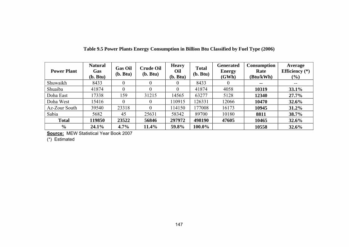
147

Table 9.5 Power Plants Energy Consumption in Billion Btu Classified by Fuel Type (2006)

Power Plant Natural

Gas (b. Btu)

Gas Oil (b. Btu)

Crude Oil (b. Btu)

Heavy Oil

(b. Btu)

Total (b. Btu)

Generated Energy (GWh)

Consumption Rate

(Btu/kWh)

Average Efficiency (*)

(%) Shuwaikh 8433 0 0 0 8433 0 -- -- Shuaiba 41874 0 0 0 41874 4058 10319 33.1% Doha East 17338 159 31215 14565 63277 5128 12340 27.7% Doha West 15416 0 0 110915 126331 12066 10470 32.6% Az-Zour South 39540 23318 0 114150 177008 16173 10945 31.2% Sabia 5682 45 25631 58342 89700 10180 8811 38.7%

Total 119850 23522 56846 297972 498190 47605 10465 32.6% % 24.1% 4.7% 11.4% 59.8% 100.0% 10558 32.6%

Source: MEW Statistical Year Book 2007 (*) Estimated

Figure 9.1 Power Plants Cosumption by Fuel Type

24.1%

4.7%

11.4%59.8%

N. Gas Gas Oil Crude Oil Heavy Oil

Table 9.6 CO2 Emissions from Fuels Used in Kuwait Power Plants

Fuel CO2 Emitted (lbs/million Btu)

CO2 Emitted (kg/GJ)

Natural Gas 117.1 49.9 Fuel Oil 161.4 68.8

Source: US EPA web site www.epa.gov/appdstar/pdf/brochure/pdf

Table 9.7 - Annual Reductions of CO2 Emissions

Year Saved Electrical Energy (GWh)

Saved Thermal Energy (billion

Btu)

CO2 Reduction (1000 lb)

CO2 Reduction

(1000 tonne) 2010 3139 33141.6 4982005.3 2259.82 2011 3482 36763.0 5526391.4 2506.75 2012 3518 37143.0 5583528.1 2532.67 2013 3571 37702.6 5667646.1 2570.83 2014 3633 38357.2 5766048.2 2615.46 2015 3718 39254.6 5900954.4 2676.66 2016 3833 40468.8 6083474.5 2759.45 2017 3962 41830.8 6288214.4 2852.32 2018 4111 43403.9 6524697.0 2959.58 2019 4263 45008.8 6765940.9 3069.01 Avg. 3723.0 39307.4 5908890.0 2680.3 Total 37230.0 393074.3 59088900.2 26802.5

148

9.5 Summary

In this Chapter, the identified DSM options are analysed regarding their

economical and environmental impacts. The analysis has arrived to several conclusions,

including:

First, the required investment rates, for the identified DSM options, are

relatively modest, ranging from 100,000 to 2,500,000 US$ annual investment by the

end of 2019.

Second, from the total resource cost perspective, most of the DSM options are

strongly cost-effective. Table 9.8 shows the economic parameters for all types of

dwellings classified by DSM option. The most cost-effective option is the increase of

thermostat set-point (DSM1), and the least cost-effective is the use of efficient end-use

equipment (DSM5).

Third, DSM4, The use of high quality roof and wall insulation, is not cost-

effective (in case of apartments, giving a negative B/C ratio. This option may need more

contribution from the customer and/or less cost sharing from the Utility (MEW).

Fourth, DSM options, through a dedicated programme, can have a significant

impact on GHG emissions, at relatively modest costs. By the year 2020, the sum of

potential CO2 reductions may reach 26.8 million tonne. The cost of achieving these

savings is approximately US$351 million.

Finally, significant policy changes will be needed to achieve these impacts,

including gradual tariff adjustment, more involvement by Utility, or government, and

the creation of sustainable DSM programmes.

Table 9.8 – Economic Parameters of DSM Options (2010 – 2019) (Dollars in $1000, Present Value)

DSM Option ID Programme

Costs Resource Savings

Net Benefits

B/C Ratio

Thermostat Resetting from 75 to 78 o F DSM1 1067 215321 214254 200

Replacing Incandescent Bulbs to CFL DSM2 5500 212552 207052 37.7

Upgrade A/C Equipment to Efficient Units with EER ≥ 11 DSM3 4406 140140 135734 30.8

High Quality Wall and Roof Insulation DSM4 1316 49540 48224 36.6

Use Energy Efficient End-Use Equipment DSM5 6113 19454 13432 2.2

Tariff Increase DSM6 25947 243640 8.4 217643 Total 44349 454753 410404 9.3

149

The average amount of CO2 reductions per year is approximately 2.68 million

tonne, and the aggregate sum of these reductions may reach 26.8 million tonne by the

end of 2019. This mitigation of CO2 could achieve an annual income of approximately

US$ 38.9 millions.

150

Chapter 10

Conclusions and Recommendations

10.1 Conclusions

Kuwait is among the fastest growing countries in the Gulf, and the electricity

demand is growing even faster than the country’s population. Kuwait has one of the

largest per capita consumption in the world, reaching 13061kWh in 2006 (MEW, 2007).

The power sector in Kuwait is not commercially viable, due to the current under-pricing

policy and heavily subsidized tariff.

The core objective of this thesis is to answer the following question: What are

the potential impacts of identified DSM measures on peak demand and energy

consumption of the residential sector, and what are the economic and environmental

benefits of these impacts?

To answer this question, a practical and a theoretical framework were

developed. The practical framework includes detailed energy audits and measurements

for selected typical models of residential dwellings (villas, apartments and traditional

houses). The theoretical framework includes simulation process for audited dwellings,

the use of Analytic Hierarchy Process to prioritize DSM options and conducting

financial spread sheet analysis to estimate the economic and environmental benefits.

Moreover, the methodology included the development of baseline scenario and demand

forecast for the period 2010 to 2019 (inclusive).

The residential sector in Kuwait consumes about 65% of total electricity

consumption, and is characterized with inefficient use of energy due to several factors,

including very cheap energy price and lack of awareness.

The major findings of this research study are:

• The research showed that a DSM portfolio consisting of seven identified

measures, and through a dedicated programme, could have substantial

reductions in energy consumption and peak demand as follows:

• DSM1: Increasing thermostat setting by 3 degrees (from 75 0 F to 78 0 F), is the

most cost-effective option for the utility and at no cost for the consumers. This

option could achieve accumulated energy savings of about 1278 GWh across the

151

period of forecast and the average peak demand reduction per year was

estimated at 156 MW. The total net accumulated savings is approximately US$

214 million, and the benefit/cost of the programme is about 200.

• DSM2: Replacement of about 80% of the widely used incandescent lamps of

rated power 40 W and 100 W to CFL of rated power 7W and 25W respectively,

could achieve savings in energy up to 1351 GWh, and reductions in peak

demand 184 MW in average for all types of dwellings. Even with 50% cost

sharing with the customer, the utility could achieve a B/C ratio of about 38.

• DSM3: Upgrading existing A/C systems to more efficient types with EER ≥ 11,

instead of 8.5 – 9.5 currently used. The potential energy savings may reach 574

GWh during the forecast period, and the average peak demand reduction is 95

MW per year. The estimated B/C ratio of this option is approximately 31.

• DSM4: The use of light coloured roofs and walls with high insulation material.

The results of analysis indicated that this option could achieve a total energy

savings of 79 GWh, and total benefits of about $48 million, with B/C ratio 37.

• DSM5 (Combined with DSM7): The use of energy efficient end-use equipment,

the application of labels and standards. The results of research indicated that this

option is the least cost-effective with B/C ratio 2.2 and the achieved energy

savings across the 10 years period of forecast is approximately 157 GWh and the

average reduction in peak demand per year is 8 MW.

• DSM6: Tariff increase; gives in the average 3110 GWh of saved energy and 226

MW of peak demand reduction per year, assuming the cost of DSM programme

estimated at US¢ 0.6 per kWh of saved energy and the price elasticity is -0.1.

The overall B/C ratio was estimated at 8.4.

The potential overall energy savings and peak demand reductions that could be

achieved with simultaneous implementations of all seven DSM options are

shown in table 10.1 in Appendix 10.

The research showed that the total accumulated energy savings across the

forecast period was estimated at approximately 34549 GWh, and the total peak demand

152

reductions during at the end of forecast (2019) reaches 1530 MW representing 8.9% of

the overall peak load.

With respect to the type of dwelling, the research also indicated that the total net

revenues for the utility were estimated at: $292 million for villas, $79 million for

apartments and $47 million for traditional houses.

One of the important indicators showed as a result of implementing the

identified DSM measures is the positive environmental impact that could be achieved

by reducing CO2 total emissions by approximately 26.8 million tonne across the

forecast period (2010-2019), which could achieve an annual income of about US$38.9

million.

The thesis recognized the barriers and difficulties which could be met for the

implementation of identified DSM measures, and stressed the importance of continuous

adaptation and institutional learning in the implementation process.

Integrated DSM policy recommendations were formulated, including gradual

tariff adjustment, and more involvement by the utility, or government, in the creation of

sustainable DSM programmes.

10.2 Barriers to DSM Implementation

One of the fundamental steps necessary to enable successful implementation of

any strategy, including DSM, is the need to understand the barriers confronting it, and

how to overcome them.

Experience in DSM by many countries, had shown the existence of some

barriers facing its implementation; namely: energy pricing, the bias towards supply

options coupled with lack of awareness, institutional, technical, financial and

administrative problems. Several of the more traditional barriers are self-evident, and

are described briefly below.

• Energy Pricing:

Low electricity price is likely to be a key barrier to uptake DSM implementation

in most of the developing countries, particularly in Kuwait, where consumers have

historically faced low unit price of electricity. Although significant progress has been

made in reducing energy subsidies in developing countries, subsidies in Kuwait still

remain as high as 5 times the current energy price.

153

• Bias Towards Supply Options:

The traditional planning mind set tends to associate greater credibility with

highly centralized power plants and does not favour investments in DSM and energy

conservation measures or decentralized options of electricity production. There should

be some incentives for electric utility to invest in DSM / EE in order not to be "supply

focussed".

• Lack of Awareness:

Consumers are frequently unaware of practices and technologies available for

energy conservation. They may be operating their electrical equipment incorrectly or

wastefully. For example, residential consumers might place their air conditioning in

direct sunlight, which is very severe in Kuwait, and this will increase its electricity

consumption.

In many cases, customers do not understand the range and benefits of air

conditioning system efficiency. Contractors tend not to be trained effectively in key

elements of proper installation or duct sealing, and have little incentives to become

more knowledgeable and aware of energy efficiency.

An important role of any DSM strategy is to increase awareness in such matters

and to bring knowledge and understanding into the various sectors. This will be

achieved through awareness campaigns, demonstration programmes, audits and

education, and public building sector energy efficiency implementation initiatives. Use

of the mass media and electronic options such as websites will be fully explored to

publicise energy-saving tips, energy management tools and best practice methods.

• Institutional and Legal Barriers:

DSM programmes and plans for energy efficiency strategies are complex and

need an appropriate institutional setting in order to be conceived and implemented.

Frequently, planning agencies suffer from the lack of personnel with good knowledge of

the behaviour of the energy market and how to implement policies to alter existing

trends of energy consumption and their evolution. At the same time the personnel need

to understand the several existing options on the supply side as well. Decisions have to

be taken concerning capital investments, and operating costs of a number of

154

alternatives. These alternatives, usually, take into account several projections of future

prices, load growth, and interest rates. These tasks require technical skills and tools so

that the potential for DSM measures are properly evaluated and the instruments to

implement them conceived.

Legal barriers frequently limit the scope of the planning activities of the electric

utilities (in Kuwait, the concerned departments in the MEW). For example, the electric

utilities in most of the developing countries are usually legally defined as being

responsible for supplying electricity only, and are required to make investments only in

the power sector.

Legal accounting procedures impede electric utilities from considering

investments in their consumer' facilities as part of the utility investment, and therefore

such investments cannot be taken into consideration when rates are calculated, for

example.

• Technical Barriers:

In many cases, the DSM energy efficiency opportunities depend on new

technologies which might not be available in some countries or regions. Product

availability is important in order to create a sustainable market for the technologies

being introduced. Most of the end-use equipment in Kuwait are imported, but ongoing

technical support needs to be available locally; other wise lack of maintenance and

support will also constitute a barrier for success in implementing the DSM options.

The quality of equipment being locally produced (or imported) is also important

to guarantee the good performance of the electrical system as a whole. For example, the

selection of electronic ballasts for fluorescent lamps, should not only save energy, but

also must satisfy minimum requirements for the level of harmonics and power factor.

The technical infrastructure in Kuwait, in particular the lack of individual

control of air conditioning and lighting, prevents fast and simple energy conservation

measures like turning off unused devices. Changes in infrastructure will require some

lead-time.

• Lack of Information:

Consumers often lack information regarding the costs and benefits of

technologies or services that deliver higher energy efficiency. Even when information is

155

provided by technology suppliers, consumers face difficulties in evaluating the

applicability of claims made for particular product or service.

The lack of substantial data bases restricted the scope of the research that could

be completed in a reasonable length of time. Data bases are needed both for energy

consumption in Kuwaiti buildings and for housing stock classified by type of building.

Other barriers exist for individual air conditioning related measures such as the

perceived aesthetics of light-coloured or reflective roofs, and lack of knowledge of the

cost effectiveness of insulation or radiant barriers.

Lack of knowledge and interest among builders regarding efficient building

techniques.

Lack of knowledge among customers and contractors that many A/C systems are

not correctly sized or installed and that this have impacts on energy cost and comfort.

10.3 Funding and Incentives

• Funding is an important factor in the diffusion of DSM programme. MEW can

fund some programmes and from whom significant demand reduction takes

place; the money can be recovered in installations along with monthly bills.

• Some countries have introduced incentives for buildings that perform better than

regulatory standards. Incentives could be offered in the form of subsidies for

investments in energy efficiency based on projected annual energy saving. Tax

credits are another form of incentives used for the same purpose. Analysis of

such approaches suggests that subsidies at the design and construction stage

have substantially greater impact on building performance than incentives based

on operating costs, such as energy taxes.

10.4 Recommendations

The conclusion of the present work indicates the urgent need, for the residential

sector in Kuwait, to direct efforts toward upgrading residential energy efficiency and

take the steps for the implementation of a pilot DSM programme for the sector. In view

of such needs and in line with the need for developing a more sustainable energy sector

as well as sustainable buildings, the following may be recommended:

The government of Kuwait should give serious consideration to the adverse

effects of the current energy consumption trends, particularly in the residential sector,

156

on both the economy and the environment. The country should move towards more

sustainable energy patterns through the implementation of appropriate policy,

regulatory and technological DSM measures.

• It is highly important to create a DSM unit within MEW or MOP to plan and

manage all further DSM activities to ensure a co-ordinated approach. As DSM

has a strong planning component, MOP would provide the appropriate

institutional background for such a DSM unit.

• The first and most important task, for the DSM unit would be the establishment

of a reliable statistical database and the commissioning of the research studies

and surveys required to provide the basis for a successful DSM strategy. This

will include the improvement of consumer statistics in MEW, as well as the

completion of research results already available by KISR.

• Establishing a reliable database and data analysis are the pre-requisites for the

development of a DSM strategy. DSM measures should only be introduced

when their impact can be predicted with sufficient accuracy.

• A least cost planning approach can ensure that energy efficiency and DSM have

a level playing field with supply options. The MEW should adopt this approach

while approving new capacity additions. This could include Bidding for DSM.

• In assessing potentials and developing energy efficiency DSM projects for

residential sector, the following has to be considered:

a. Special attention has to be given to the no cost/low cost energy

conservation measures such as housekeeping (e.g. thermostat re-

setting and switching off un-used equipment). Low cost measures

distributed to many end-users can result in a large savings normally

difficult to achieve without large capital investment, provided the

project is managed effectively.

b. Detailed energy audits are required, especially for private houses of

high consumption (more than 9000 kWh/month), which may come

up with cost-effective DSM projects.

c. Priority is to be given for adopting simple, locally handled and

sustained technologies rather than high-level sophisticated systems

with a short-term sustaining period.

157

• Demonstration projects are important tools and successful ways of convincing

rate-payers of the effectiveness of energy efficiency DSM measures.

Demonstrations should focus on technologies and end-uses that are relevant to

the rate-payers. For residential sector, technologies to be considered should

include energy-efficient cooling systems, lighting, and energy-efficient

appliances.

• The high transaction costs of DSM programme by the utility (MEW) could be a

barrier. However, any DSM programme should have a positive effect on the

utility and have significant saving potential. The challenge, also, is to generate

consumer participation / interest since they pay highly subsidised tariff.

• The government should form joint working groups of representatives of the Ministry of Electricity and Water (the sole provider of electricity) and representatives of the Public Authority of Housing Welfare (a major provider of the buildings housing), with a view to verifying the application of regulations and regulations to improve residential building standards (selection of building materials, improvement of energy efficiency and efficient buildings, etc.).

• Innovative Programme Design:

Focused DSM programmes that target the barriers involved and have low

transaction cost need to be designed. A large number of pilot programmes need to be

tried with different institutions, incentives, and implementation strategies. KISR can

play an important role in these programmes. A few suggestions are included here:

10.4.1 Efficient Lighting Initiative

The use of energy efficient lamps has a large potential of savings in Kuwait,

since most of the residential consumers use conventional incandescent lamps. Electric

utility of Kuwait (MEW) should launch pilot efficient lighting initiatives in towns /

cities. Features should include warranties by manufactures or suppliers, incentives and /

or deferred payment through utility bill savings

One of the best and successful DSM programmes in high efficiency lighting was

implemented in Thailand during 1993 to 2000. The programme was the primary reason

for the manufacturers to shift production from the normal fluorescent lamps to the

energy-efficient "thin tube" (T-8) lamps60.

Thailand probably has the most extensive experience in programme evaluation,

having completed a detailed evaluation costing US$4 million and engaging multiple

158

consultants to assist in the DSM effort. Thailand's experience has underlined the

importance of a concurrent evaluation process being an integral part of DSM61.

International examples in efficient lighting are also available at:

www.efficientlighting.net.

10.4.2 Green Building Initiative62

Although the concept of green building (GB) is relatively new, today, it is one of

the fastest growing building and design concepts. Green building is a "whole-system"

approach for designing and constructing buildings that conserve energy, water, and

material resources and are healthier, safer and more comfortable.

In practical terms, green buildings are designed and constructed to:

• Incorporate energy efficiency features (use natural ventilation and lighting, good

insulation, high efficiency lighting, green roofs, solar or geothermal energy).

• Incorporate water efficient features (e.g. use waterless urinals, low-flow faucets

and toilets, etc.).

• Re-use existing building structures and/or building materials; reduce and recycle

waste materials.

• Preserve natural vegetation, and reduce disturbance to landscape and habitats, in

order to maintain bio-diversity and preserve ecological integrity.

• Incorporate sustainable, healthy, locally made or harvested non-toxic materials

and features into buildings (e.g. FSC or recycled wood, low VOC carpets, paint

and composite wood products, previously used or recycled materials).

• Incorporate flexible design and durability whenever possible (e.g. movable walls

that don't require renovation to reconfigure).

And for operation and management, green buildings:

• Use green waste management practices.

• Use non-toxic cleaning products.

• Monitor and commission building installations and building operations to

ensure that planned targeted designs are met with results.

159

Recent research confirms that it makes good economic sense for governments to

support green buildings design and practice. In the United States, a 2003 report to the

California Sustainable Building Task Force predicted:

While the environmental and human health benefits of green buildings

have been widely recognized, minimal increases in up-front costs of 0 to

2 percent to support green building design will result in life cycle

savings of 20 percent of total construction costs – more than 10 times

the initial investment63.

Several green building rating systems are now in use to evaluate and certify

green buildings. Examples of these rating systems are: LEED (Leadership in Energy

and Environmental Design), developed by the US Green Building Council (USGBC) as

a national standard for high performance sustainable buildings, BREEAM (BRE

Environmental Assessment Method), created in UK, in 1990 with the first two versions

covering offices and homes, and LEED India, established and administered by the

Indian Green Building Council (IGBC) under licence agreement with the USGBC.

10.5 Future Research Work The following research topics are highly attractive and important for Kuwait:

1. Integrating Demand Side Management Programmes into Resource Plan

of Kuwait

DSM has become more integral to utility strategic plans, and experience with

DSM field implementation has grown substantially over the past few years. During this

time, most utilities have emphasized programme selection, design, and implementation.

In Kuwait, the integration of DSM into resource planning is important to be

investigated and studied in depth.

Equally important is obtaining the assurance that DSM programmes are

effectively designed and efficiently implemented and that they provide valued services

to customers.

The research addresses and investigates the main Integrated Resource Planning (IRP)

options, including, but not limited to, the following action:

160

• Integrating DSM programmes with supply expansion. The key element of

the IRP process is to bring the economic evaluation of energy efficiency into

an equal basis with supply expansion.

• The opportunity of integrating private producers and cogeneration with

Utility generation. In Kuwait, as most of the developing countries, the high

rate of growth in the demand for electric service will still require expansion

of the central generating capacity. However, the potential of introducing

small-scale generating units, such as industrial stand-by generators and

cogeneration could be cost-effective. A further goal of resource planning is

thus to allow the evaluation of such sources on an equal basis with central

supply expansion.

• Integrating public total resource perspective with the utility perspective.

• Integrating environmental impacts and risks with cost analysis.

Environmental issues are likely to be more important in the future as

concerns over the regional and global environment, including the potential

threat of global climate change, become increasingly serious. The costs of

environmental emissions from electricity supply are put of the costs avoided

through selection of DSM and renewable supply sources. These costs can be

quantified either as emission charges actually paid by the utility, or they can

be proxy values used to prioritize and select DSM and supply options in the

IRP process.

2. The challenge for the development and diffusion of renewable energy

technologies: Solar Power in Kuwait

By burning fossil fuels, electrical power generation affects not only the

environment directly and the global climate potentially but the nation's economic

strength and its prospects for energy security as well. Using solar power, wind power,

and other forms of renewable energy to generate electricity is one response to these

concerns.

The research is aiming to investigate the potential of utilization of solar power in

Kuwait, particularly in all sectors of Kuwait.

161

Kuwait, as all countries in the Middle East, enjoys excellent solar resources with

an annual average of global solar radiation approximately 6.2 kilowatt hour per square

meter (kWh/m2) per day (UN ESCWA Report, NY, 2001). The annual average of total

cloud covers can be as low as less than 10%.

With the trend of high electricity demand in Kuwait, and under the conditions of

environmental concerns, there is a need for the development and dissemination of

renewable energy, particularly solar power.

The study has to assess the institutional framework for solar power

development, and areas of potential applications. Assessment of national capabilities in

the field of education, training, information and certification is also important to be

investigated.

It is important in the research, to include the optimization of solar cooling

systems for buildings, solar thermal power desalination systems, and solar water heating

systems. Moreover, the opportunity of manufacturing low-cost solar water heaters for

residential use, from locally available material, is also important.

162

REFERENCES 1Solar Energy Research Institute. DSM pocket guidebook, Volume 1: Residential Technologies (SERI/TP-254-4098A. CO (USA): Solar Energy Research Institute; 1991.

2Solar Energy Research Institute. DSM pocket guidebook, Volume 1: Commercial Technologies (SERI/TP-254-4098B. CO (USA): Solar Energy Research Institute; 1991.

3Solar Energy Research Institute. DSM pocket guidebook, Volume 2: Industrial Technologies (SERI/TP-254-4098C. CO (USA): Solar Energy Research Institute; 1991. 4The Energy Information Administration (EIA), Demand Side Management Programme, annual report, 1999, Stockholm: International Energy Agency, 2000. 5Joskow P., Marron D. "What does a Negawatt really cost" Evidence from utility conservation programs. Energy J., 1993. 6Ali E. H. Hajiah "Energy Conservation Program in Kuwait": A Local Perspective, Department of Building and Energy Technologies, KISR 2007, Kuwait. 7Al-Marafie, A.M.R. R.K. Suri and G.P. Maheshwari, 1989. Energy and Power Management in Air-conditioned buildings in Kuwait. Energy 9 557-562. 8R.K. Suri, G.P. Maheshwari, and M. Sebzali, 1984. " Cool Storage Assisted Air-conditioning Systems". Department of Building and Energy Technologies, KISR, Kuwait. 9Essam Al-Sayed O. Assem " Kuwaiti Code for Energy Conservation in Buildings". Department of Building and Energy Technologies, KISR 2003, Kuwait.

10D. Al-Nakib "Energy Conservation Opportunities for Lighting Systems in Office Buildings". Department of Building and Energy Technologies, KISR 2002 , Kuwait. 11The Ministry of Energy (Electricity & Water), State of Kuwait, Statistical Year Book, 2007. 12International Energy Agency (IEA), Key World Energy Statistics-2006, "Selected Energy Indicators for 2004". 13IEA, World Energy Outlook 2005, Middle East and North Africa Insight (Chapter 6), 2007. 14Energy Information Administration (1995). U.S. Electric Utility Demand Side Management 1994. Washington DC, EIA. 15Electric Power Research Institute. Demand –Side Management, 5 volumes. AE/EM-3597. Palo Alto 2002, CA, USA.

163

16The International Institute for Energy Conservation- ECO II, DSM Best Practices Guide Book, 2005. 17Gellings, C.W. and J.H. Chaberlin (1993), Demand Side Management: Concepts and Methods. Liburn, GA, USA, the Fairmont Press, Inc. 18United Nations Environmental Programme (1992). Agenda 21. New York, United Nations. 19S. Boyle, DSM Progress and Lessons in the Global Context. International Institute for Energy Conservation – Europe, London, UK, 1996. 20National Resource Defence Council, Demand-Side Management in China"- Appendix IV, International Experience with Demand-Side Management, October, 2003. 21Sioshansi, F. P. (1995). "Demand-Side Management: The Third Wave. "Energy Policy 23(2): 111-114. 22National Resources Defence Council (NRDC), Demand-Side Management in China, Appendix IV, "International Experience with DSM", October, 2003. 23UNEP. Tools and Methods for Integrated Resource Planning. November, 1997. 24"DSM in Thailand : A Case Study" . UNDP, World Bank, Energy Sector Management Assistance Programme (ESMAP), October, 2000. 25J. Singh and C. Mulholland. DSM in Thailand: A Case Study, October, 2000. 26Energy Conservation and Environment Protection. USAID Project (1989-1998), Cairo, Egypt. 27Proceedings of the: "DSM and the Reforming Energy Market Conference", December, Cairo, Egypt, 1997. 28Ministry of Planning, State of Kuwait "Future Expansion in Generation and Transmission for the State of Kuwait", Final Report, January 2000. 29Ministry Of Planning, Census and Statistical Sector, www.Kuwait-info.com. 30Statistical Abstracts in 25 Years. Special Issue 1990 and Annual Statistical Abstracts, 1998. 31Al-Qabas Newspaper, Kuwait, 12 August, 1999. 32Golden, B., Wasil, E. and Harker, P. (eds.) 1989. The Analytic Hierarchy Process: Applications and Studies, Springer Verlag, New York.

164

33Ahmed A. Al-Mulla, PhD., Energy Building Technologies Department, KISR, Kuwait. (An expert, personal contact) 34A.R. Khozam, PhD., Energy Expert, Consultant, Energy Efficiency Improvement and GHG Project (GEF/UNDP), Cairo, Egypt (Director of a Pilot DSM Programme in industrial sector from 1994 to 1998).(An expert, personal contact) 35I. Yassien, PhD., Ministry Of Electricity and Energy, Director of EEIGGR Project (GEF/UNDP), Cairo, Egypt. (The project supervised and implemented several DSM projects).(An expert, personal contact) 36Stephen Wiel, J.E. McMahon, " Energy – Efficiency Labels and Standards: A Guidebook for Appliances, Equipment, and Lighting", 2nd Edition, 2005. 37Lahmeyer International GmbH – The Associated Engineering Partnership , LI/GE 7 / 260046, January 2000. 38Saaty TL, The Analytic Hierarchy Process, New York, McGraw-Hill, 1980. 39Saaty TL How to Make a Decision: The Analytic Hierarchy Process, European Journal of Operational Research, North Holland, 1990, -48: 9-26. 40Expert Choice, Inc., "Expert Choice Software and Manual". 4922, Elsworth Ave., Pittsburgh, PA, 15213, USA. 41www.expertchoice .com, Expert Choice, Inc. (5). 42Forman, EE. And Selly, M. 2001. Decision by Objectives. Expert Choice, Inc. USA. 43The Economic Impact of Changing the Structure of Electricity Pricing in Kuwait. Final Report, 1987. 44Suozzo, M. and Nadel, S. 1996. What Have We Learned from Early Market Transformation Efforts?, ACEEE, August. 45Packcy, Daniel, J. 1993, "Market Penetration of New Energy Technologies". U.S. Dept. of Energy, National Renewable Energy Laboratory. 46Rogers, E.M. The Diffusion of Innovations, 5th Edition, 2003 47Dmitry Kucharavy, Roland De Guio, “Logistic Substitution Model and Technological Forecasting", LGECO, France 2005. 48"Best Practices in Technology Deployment Policies", Hans Nilsson 2001. 49KISR, The Economic Impact of Changing the Structure of Electricity Pricing in Kuwait. Final Report, June 1987.

165

50G. Papagiannis, A. Dagoumas, N. Lettas, P. Dokopoulos, 2008. Economic and environmental impacts from the implementation of an intelligent demand side management system at the European level. Energy Policy, Volume 36, Issue 1, Pages 163-180

51UNEP, Joel N. Swisher, at al., "Tools and Methods for Integrated Resource Planning". November 1997. 52The Tellus Institute, “Best Practice Guide: Integrated Resource Planning For Electricity”, Prepared for: Energy and Environment Training Program, Office of Energy, Environment and Technology Global Bureau, USAID Office of Energy. 53J.N. Sheen “Economic Profitability Analysis of Demand Side Management Program”, Dept of Electrical Engineering, Taiwan, 2005. 54C. P. Maheshwari, R. Al-Murad, “Impact of Energy Conservation Measures on Cooling Load and Air-conditioning Plant Capacity”, Building and Energy Technologies Dept., KISR, Kuwait, 2000. 55Martin Kushler, Dan York and Patti Witte, Five Years In: An Examination of the First Half-Decade of Public Benefits Energy Efficiency Policies, ACEEE, April 2004, p.30. 56Nadel, S., Wolcott, D., Smith, P., Flaim. T., 1990. “A Review of Utility Experience with Conservation and Load Management Programs for Commercial and Industrial Customers”. 57Hirst, E., J. Reed, 1991. “Handbook of Evaluation of Utility DSM Programs,” ORNL/CON-336, Oak Ridge National Laboratory. 58“Public Service New Mexico Electric Energy Efficiency Potential Study”/ Methodology.

59W.W. Clark II, A Sowell, et al, “The Standard Practices Manual: The Economic Analysis of Demand Side Programs and Projects in California”, USA, 2002. 60”DSM in Thailand: A Case Study”, UNDP, World Bank, Energy Sector Management Assistance Program, Oct. 2000. 61”DSM in the Electricity Sector: Urgent Need for Regulatory Action and Utility-Driven Programmes”. Report by: Prayas Energy Group (Pune), February, 2005. 62S. Rutherford, "The Green Buildings Guide", West Coast Environmental Law.

63LEED India / Terri Griha (http: // www.teriin.org).

166

167

APPENDICES

Design Parameters: City Name .......................................................................... Kuwait City Location ...................................................................................... Kuwait Latitude ............................................................................................ 29.2 Deg. Longitude ........................................................................................ -48.0 Deg. Elevation ........................................................................................ 180.0 ft Summer Design Dry-Bulb ............................................................. 117.0 °F Summer Coincident Wet-Bulb ................................. 69.0 °F Summer Daily Range ....................................................................... 27.7 °F Winter Design Dry-Bulb .................................................................. 38.0 °F Winter Design Wet-Bulb ................................................................. 31.9 °F Atmospheric Clearness Number ...................................................... 1.00 Average Ground Reflectance ........................................................... 0.20 Soil Conductivity .................................................. 0.800 BTU/(hr-ft-°F) Local Time Zone (GMT +/- N hours) ............................................... -3.0 hours Consider Daylight Savings Time ....................................................... No Simulation Weather Data ......................................... Kuwait City (Avg) Current Data is ............................................ 2001 ASHRAE Handbook Design Cooling Months ..................................... January to December Design Day Maximum Solar Heat Gains (The MSHG values are expressed in BTU/ hr-ft²)

Appendix to Ch 4

168

Month N NNE NE ENE E ESE SE SSE S January 24.6 24.6 33.1 112.3 185.7 228.4 253.4 248.6 238.9 February 28.2 28.2 74.6 148.5 213.6 245.1 246.1 225.7 209.8 March 32.1 34.5 120.2 185.2 224.8 241.3 220.7 184.4 161.5 April 36.0 79.5 153.8 205.4 225.9 214.6 181.5 129.4 100.0 May 39.6 110.8 173.5 212.4 219.6 193.7 148.2 87.8 61.8 June 51.4 120.0 180.3 212.8 213.5 182.4 133.1 72.1 51.2 July 41.1 110.1 172.9 208.6 213.2 189.5 144.1 84.7 59.9

August 37.6 77.3 150.9 198.3 215.9 208.2 174.5 124.4 96.3 September 33.4 34.8 111.5 177.5 215.2 228.9 214.0 180.3 159.0

October 29.2 29.2 69.3 148.7 200.6 236.0 238.4 219.7 205.7 November 25.1 25.1 34.5 109.6 179.9 229.8 245.9 243.3 237.4 December 23.1 23.1 23.1 92.4 171.9 221.3 250.7 252.1 247.2

Month SSW SW WSW W WNW NW NNW HOR Mult January 248.7 253.4 227.6 185.5 112.8 32.5 24.6 187.8 1.00 February 225.2 245.4 245.7 212.8 146.5 75.2 28.2 226.4 1.00 March 184.3 219.7 241.7 227.4 181.7 120.1 36.5 259.0 1.00 April 128.0 178.6 218.0 225.2 199.7 154.2 82.1 275.1 1.00 May 86.4 146.3 196.6 217.3 208.4 174.5 113.6 278.7 1.00 June 70.8 132.3 185.4 210.2 210.6 181.0 124.1 277.0 1.00 July 83.9 143.3 191.2 210.6 206.9 173.0 112.5 274.0 1.00

August 123.0 171.8 210.0 217.2 193.2 150.1 81.7 268.9 1.00 September 180.5 214.2 228.3 218.9 176.0 106.8 37.6 252.2 1.00

October 219.9 238.9 235.1 202.4 149.0 67.9 29.2 224.4 1.00 November 244.5 246.7 229.5 176.5 112.9 32.6 25.1 188.9 1.00 December 252.8 249.6 223.6 165.3 98.8 23.1 23.1 172.3 1.00

Mult. = User-defined solar multiplier factor.

169

QUESTIONNAIRE (RESIDENTIAL BUILDING) )مبنى سكنى(نموذج استبيان A. GENERAL INFORMATION معلومات عامة: Person in Charge: المدير المسئول Name: الاسم: Tel. : تليفون: E-mail: البريد الالكتروني: B. BUILDING CONSTRUCTION وصف المبنى: 1. Orientation: Facing ………………………… الاتجاه:

2. Total land Area (m2 ): اجمالي مساحة الارض

):2م(

3. Total Living (Closed) Area (m2 ): يشة اجمالي مساحة المع

):2م( 4. Total Roof Area (m2 ):

اجمالي مساحة السطح ):2م(

5. Number of Floors: عدد الادوار:

170

6. External Opaque Wall Area (m2 ): مساحة الحوائط

الخارجية 7. Total Window Area (m2 ):

No. x Area of each window = :مساحة الشبابيك …………………………

8. Window Glass Type: زجاج الشبابيك: 9. Landscape Area (m2 :المساحة :( 10. Swimming Pool Area (m2 ): مساحة حمام السباحة: 11. Wall Insulation: YES NO عزل الحائط: TYPE: 12. Roof Insulation: YES NO عزل السقف: TYPE:

13. Window-to-wall Ratio (%): نسبة مساحة النوافذ الى

:الحوائط 14. Floor-to-floor Height (m): ارتفاع السقف : 15. Occupancy: ……. Persons عدد الافراد:

171

C. ENERGY CONSUMPTION: استهلاك الطاقة. ج Year: السنة

Month Electricity Elec. Bill N. Gas Gas Bill (kWh) (LE) (m3) (LE)

استهلاك الشهر الكهرباء

فاتورة رباءالكه

استهلاك الغاز الطبيعي

فاتورة الغاز الطبيعي

January February March April June July August September October November December

Total

172

D. AIR CONDITIONING SYSTEM نظام التبريد والتكييف Type: الطراز:

Central: Package Air Cooled Chilled Water Cooling

تبريد بالمياه تبريد بالهواء مرآزي Rated Capacity: :Ton القدرة Btu/hr: Split: :Qty منفصل Capacity: Window: :Qty شباك Capacity: Thermostat Setting: …… 0 C درجة الحرارة:

Average Daily Operating Hours: عدد ساعات التشغيل

:اليومية Heating in Winter: YES NO التدفئة في الشتاء If YES - Heating Months ….. (November - February) ? شهور التدفئة

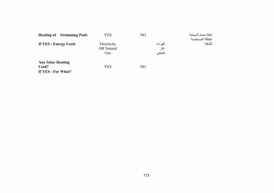
173

Heating of Swimming Pool: YES NO تدفئة حمام السباحة

If YES - Energy Used: Electricity آهرباء الطاقة المستخدمة

للتدفئة

OR Natural

Gas غاز طبيعي

Any Solar Heating Used? YES NO If YES - For What?

174

F. END-USE EQUIPMENT

Equipment Type Qty Size Rated Power

Operating Hours Remarks (ملاحظات)

(W)

Refrigerator

Freezers

Water Heater

E. LIGHTING SYSTEM

Type Qty Rated Power

(W)

Total Power

(W)

Avg. Op.

Hours Comments (ملاحظات)

1. Lamps Incandescent 100 (لمبة فتيلة عادية)

Incandescent 60 (لمبة فتيلة عادية)

Fluorescent 1 40 Fluorescent 2 20

Halogen --- Others

2. Ballast Magnetic Electronic

3. Fixtures No. of Lamps Reflector NO 4. Dimmer

175

Washing Machine

TV Set

VCR/DVD

Electrical Fans

Vacuum Cleaner

Electric Iron

Computer + Printer

176

Appendix to Ch 5

Apartment 1 Reception 1. General Details: Floor Area ................................. 1000.0 ft² Avg. Ceiling Height ........................ 9.0 ft Building Weight .......................... 120.0 lb/ft² 1.1. OA Ventilation Requirements: Space Usage .................. User-Defined OA Requirement 1 ........................ 2.60 CFM/ft² OA Requirement 2 ........................ 20.0 CFM/person 2. Internals: 2.1. Overhead Lighting: Fixture Type ..... Recessed (Unvented) Wattage ......................................... 0.80 W/ft² Ballast Multiplier .......................... 1.08 Schedule Profile 5 2.2. Task Lighting: Wattage ......................................... 0.20 W/ft² Schedule ....................... Task Lighting 2.3. Electrical Equipment: Wattage ......................................... 0.50 W/ft² Schedule ................................ Profile 5 2.4. People: Occupancy .......................................... 2 People Activity Level .............. Seated at Rest Sensible ....................................... 230.0 BTU/hr/person Latent .......................................... 120.0 BTU/hr/person Schedule Reception Schedule 2.5. Miscellaneous Loads: Sensible .............................................. 0 BTU/hr Schedule ...................................... None Latent ................................................. 0 BTU/hr Schedule None 3. Walls, Windows, Doors:

Exp. Wall Gross Area (ft²)

Window 1 Qty.

Window 2 Qty. Door 1 Qty.

N 484.0 2 2 0 E 323.0 2 0 0 W 480.0 2 1 0

177

3.1. Construction Types for Exposure N Wall Type ....... Apartment Wall Assembly 1st Window Type Apt. Reception Window 2 1st Window Shade Type Default Shade Type 2nd Window Type . Apt. North, Window 2 2nd Window Shade Type Default Shade Type 3.2. Construction Types for Exposure E Wall Type ....... Apartment Wall Assembly 1st Window Type .. Apt. North, Window 1 1st Window Shade Type Default Shade Type 3.3. Construction Types for Exposure W Wall Type ....... Apartment Wall Assembly 1st Window Type .. Apt. North, Window 1 1st Window Shade Type Default Shade Type 2nd Window Type . Apt. North, Window 2 2nd Window Shade Type Default Shade Type 4. Roofs, Skylights:

Exp. Roof Gross Area (ft²) Roof Slope (deg.) Skylight Qty.

H 1000.0 0 0 4.1. Construction Types for Exposure H Roof Type Built-up Roof + 8" HW Concrete 5. Infiltration: Design Cooling ............................. 0.10 ACH Design Heating .............................. 0.00 CFM Energy Analysis ............................ 1.00 ACH Infiltration occurs only when the fan is off. 6. Floors: Type Floor above Conditioned Space (No additional input required for this floor type). 7. Partitions: 7.1. 1st Partition Details: Partition Type .............. Wall Partition Area ............................................. 120.0 ft² U-Value ....................................... 0.500 BTU/(hr-ft²-°F) Uncondit. Space Max Temp ......... 75.0 °F Ambient at Space Max Temp ....... 95.0 °F

178

Uncondit. Space Min Temp .......... 75.0 °F Ambient at Space Min Temp ........ 85.0 °F 7.2. 2nd Partition Details: (No partition data). Traditional House Analysis 1. General Details: Floor Area ................................. 3100.0 ft² Avg. Ceiling Height ........................ 9.0 ft Building Weight ............................ 90.0 lb/ft² 1.1. OA Ventilation Requirements: Space Usage .................. User-Defined OA Requirement 1 ........................ 20.0 CFM/person OA Requirement 2 ........................ 7.20 CFM/ft² 2. Internals: 2.1. Overhead Lighting: Fixture Type ................. Free Hanging Wattage ......................................... 0.80 W/ft² Ballast Multiplier .......................... 1.08 Schedule ................................ Lighting 2.2. Task Lighting: Wattage ......................................... 0.20 W/ft² Schedule ................................ Lighting 2.3. Electrical Equipment: Wattage ......................................... 0.10 W/ft² Schedule ..................... Electrical Eqpt 2.4. People: Occupancy .......................................... 7 People Activity Level .............. Seated at Rest Sensible ....................................... 230.0 BTU/hr/person Latent .......................................... 120.0 BTU/hr/person Schedule .................................... People 2.5. Miscellaneous Loads: Sensible .............................................. 0 BTU/hr Schedule ...................................... None Latent ................................................. 0 BTU/hr Schedule ...................................... None

179

3. Walls, Windows, Doors:

Exp. Wall Gross Area (ft²)

Window 1 Qty.

Window 2 Qty. Door 1 Qty.

NE 520.0 2 1 1 ESE 580.0 2 1 0 SW 520.0 2 0 1 WNW 580.0 2 1 1

3.1. Construction Types for Exposure NE Wall Type .............. Default External Wall 1st Window Type ....................... Window 1 1st Window Shade Type Default Shade Type 2nd Window Type ...................... Window 4 2nd Window Shade Type Default Shade Type Door Type ....................................... Door 1 3.2. Construction Types for Exposure ESE Wall Type .............. Default External Wall 1st Window Type ....................... Window 1 1st Window Shade Type Default Shade Type 2nd Window Type ...................... Window 2 2nd Window Shade Type Default Shade Type 3.3. Construction Types for Exposure SW Wall Type .............. Default External Wall 1st Window Type ....................... Window 1 1st Window Shade Type Default Shade Type Door Type ....................................... Door 1 3.4. Construction Types for Exposure WNW Wall Type .............. Default External Wall 1st Window Type ....................... Window 1 1st Window Shade Type Default Shade Type 2nd Window Type ...................... Window 4 2nd Window Shade Type Default Shade Type Door Type ....................................... Door 1 4. Roofs, Skylights:

Exp. Roof Gross Area (ft²) Roof Slope (deg.) Skylight Qty.

H 1700.0 0 0

180

4.1. Construction Types for Exposure H Roof Type ..... Default Roof Assembly 5. Infiltration: Design Cooling ............................. 0.10 ACH Design Heating .............................. 0.00 CFM Energy Analysis ............................ 0.00 CFM Infiltration occurs only when the fan is off. 6. Floors: Type Floor above Conditioned Space (No additional input required for this floor type). 7. Partitions: (No partition data). Villa Analysis – Base Case 1. General Details: Floor Area ................................. 3358.0 ft² Avg. Ceiling Height ...................... 10.2 ft Building Weight ............................ 90.0 lb/ft² 1.1. OA Ventilation Requirements: Space Usage .................. User-Defined OA Requirement 1 ........................ 20.0 CFM/person OA Requirement 2 ........................ 7.40 CFM/ft² 2. Internals: 2.1. Overhead Lighting: Fixture Type ................. Free Hanging Wattage ......................................... 1.10 W/ft² Ballast Multiplier .......................... 1.08 Schedule ................................ Lighting 2.2. Task Lighting: Wattage ......................................... 0.20 W/ft² Schedule ................................ Lighting 2.3. Electrical Equipment: Wattage ......................................... 0.20 W/ft² Schedule ..................... Electrical Eqpt 2.4. People: Occupancy .......................................... 7 People Activity Level .......... Sedentary Work Sensible ....................................... 280.0 BTU/hr/person Latent .......................................... 270.0 BTU/hr/person Schedule .................................... People

181

2.5. Miscellaneous Loads: Sensible .............................................. 0 BTU/hr Schedule ...................................... None Latent ................................................. 0 BTU/hr Schedule ...................................... None 3. Walls, Windows, Doors:

Exp. Wall Gross Area (ft²)

Window 1 Qty.

Window 2 Qty. Door 1 Qty.

N 450.0 2 0 1 S 450.0 2 2 0 E 394.0 1 0 1 W 394.0 1 0 1

3.1. Construction Types for Exposure N Wall Type .............. Default External Wall 1st Window Type ....................... Window 1 1st Window Shade Type Default Shade Type Door Type ....................................... Door 1 3.2. Construction Types for Exposure S Wall Type .............. Default External Wall 1st Window Type ....................... Window 1 1st Window Shade Type Default Shade Type 2nd Window Type ...................... Window 2 2nd Window Shade Type Default Shade Type 3.3. Construction Types for Exposure E Wall Type .............. Default External Wall 1st Window Type ....................... Window 1 1st Window Shade Type Default Shade Type Door Type ....................................... Door 1 3.4. Construction Types for Exposure W Wall Type .............. Default External Wall 1st Window Type ....................... Window 1 Door Type ....................................... Door 1

182

4. Roofs, Skylights:

Exp. Roof Gross Area (ft²) Roof Slope (deg.) Skylight Qty.

H 1722.0 0 0 4.1. Construction Types for Exposure H Roof Type ......................... Roof Assembly 5. Infiltration: Design Cooling ............................. 0.50 ACH Design Heating .............................. 0.00 CFM Energy Analysis ............................ 0.00 CFM Infiltration occurs at all hours. 6. Floors: Type Floor above Conditioned Space (No additional input required for this floor type). 7. Partitions: (No partition data).

183

APPENDIX to Ch 7 APPLICATION OF AHP IN RANKING DSM OPTIONS

1. Steps for Applying AHP. Saaty [1-4] developed the following steps for applying the AHP:

(i) Define the problem and determine its goal. (ii) Structure the hierarchy from the top (the objectives) through the intermediate levels

(criteria on which subsequent levels depend) to the lowest level which usually contains the list of alternatives.

(iii) Construct a set of pair-wise comparison matrices (size n x n) for each of the lower levels with one matrix for each element in the level immediately above by using the relative scale measurement shown in Table 1. The pair-wise comparisons are done in terms of which element dominates the other.

(iv) There are n(n-1) judgments required to develop the set of matrices in step (iii). Reciprocals are automatically assigned in each pair-wise comparison.

(v) Historical synthesis is now used to weight the eigenvectors by the weights of the criteria and the sum is taken over all weighted eigenvector entries corresponding to those in the next lower level of the hierarchy.

(vi) Having made all the pair-wise comparisons, the consistency is determined by using the eigenvalue, λmax , to calculate the consistency index, CI as follows :

CI = (λ max-n)/(n-1)

Where n is the matrix size. Judgment consistency can be checked by taking the consistency ratio (CR) of CI with the appropriate value in Table 2. The CR is acceptable, if it does not exceed 0.10. If it is more, the judgment matrix is inconsistent. To obtain a consistent matrix, judgments should be reviewed and improved.

(vii) Steps (iii) – (vi) are preferred for all levels in the hierarchy.

184

Table 1 Par-wise Comparison for AHP Preferences [1-4]

Numerical Rating Definition Explanation

9 Extremely preferred Evidence favouring this activity is of absolute affirmation

7 Very strongly preferred An activity is strongly favoured and its dominance is demonstrated in practice

5 Strongly preferred Experience and judgment suggest a strong favour over another

3 Moderately preferred Experience and judgment slightly favour one over another

1 Equally preferred Two activities contribute equally to the objective

2,4,6,8 Intermediate values When compromise is needed

Table 2 - Average Random Consistency (RI) [1-4]

Size of matrix

1 2 3 4 5 6 7 8 9 10

Random consistency

0 0 0.58 0.9 1.12 1.24 1.32 1.41 1.45 1.49

The steps mentioned above could be implemented either automatically using software, or “Expert Choice”, developed by Export Choice, Inc. [5], or manually as will be demonstrated as follows.

185

2. AHP for Identifying DSM Priority Options In this research, Saaty method of AHP will be applied as follows: Step 1: We completely define the problem and develop a hierarchy which will accurately represent the problem using the following guidelines: Level 1 – Final goal: Level 2 – Criteria used to judge alternatives Level 3 – Alternatives As shown in Figure 1, the goal is represented by high priority DSM option with optimum saved energy and peak demand reduction. In level 2, six criteria are used to evaluate DSM options (alternatives), as shown in Table 3. Each criterion has five scores (weights). These weights are provided by DSM experts.

186

Figure1 – AHP Block Diagram

Priority DSM Options with Optimum Energy Savings & PD Reductions

Saved Energy

Peak Demand Reduction

Penetration Rate

Payback Period

Technology Acceptance

High Efficiency Lighting (DSM3)

Roof and Wall Insulation (DSM4)

Efficient End-Use

Equipment

Tariff Increase (DSM6)

Standards & Labels (DSM7)

Level 1 (Goal)

Level 2 (Criteria)

Level 3 (Alternatives)

Investment Cost

Efficient A/C Equipment

(DSM2)

Thermostat Setting (DSM1)

187

Table 3 – Six Criteria Used for DSM Evaluation

Weight Criteria 1 3 5 7 9

1. Saved Energy Very low (<10%)

Low (10-20%)

Medium (20-30%)

High (30-40%)

Very High (> 40%)

2. Peak Demand Reduction

Very low (<10%)

Low (10-20%)

Medium (20-30%)

High (30-40%)

Very High (> 40%)

3. Investment Cost Very high cost

High cost Medium cost

Low cost No Cost/Very low cost

4. Payback Period Very long (>5 yrs)

Long (4-5 yrs)

Medium (2-4 yrs)

Short (1-2 yrs)

Very short (< 1 yr)

5. Penetration Level

1 - 5% per year

5 – 10% per year

10 – 20% per year

20 – 30% per year

> 30% per year

6. Technology Acceptance

Low. Acceptance

Medium. Acceptance

High Acceptance

Very High Acceptance

Full Acceptance

The weights of each criterion are based on the experience of DSM experts. Step 2: The next step is to develop matrices that compare the criteria with themselves (within level 2) and the alternatives (DSM options) with each criterion (between level 2 and level 3). Pair-wise comparisons are needed to determine the relative importance of each ratings scale category (intensity). In the hierarchy shown in Figure 1, alternative are not pair-wise compared in a rating model, rather alternatives are rated for each criterion. The pair-wise comparison matrix for the six criteria is developed in Table 4, in terms of importance of each in contributing to the overall goal. We notice in Table 4, the ones across the diagonal.

188

Table 4 - Pair-wise Comparison Matrix for the Six Criteria (With Column Totals)

SE PLR IC PBP PR TA Priority

Vector

SE 1.0 1.00 (9/9)

1.286 (9/7)

1.286 (9/7)

1.800 (9/5)

3.00 ((9/3) 0.225

PLR 1.00 (9/9) 1.0 1.286

(9/7) 1.286 (9/7)

1.800 (9/5

3.00 (9/3) 0.225

IC 0.778 (7/9)

0.778 (7/9) 1.0 1.0

(7/7) 1.400 (7/5)

2.333 (7/3) 0.175

PBP 0.778 (7/9)

0.778 (7/9)

1.0 (7/9)

1.0

1.400 (7/5)

2.333 (7/3) 0.175

PR 0.556 (5/9)

0.556 (5/9)

0.714 (5/7)

0.714 (5/7) 1.0 1.667

(5/3) 0.125

TA 0.333 (3/9)

0.333 (3/9)

0.429 (3/7)

0.429 (3/7)

0.600 (3/5) 1.0 0.075

SUM 4.444 4.444 5.714 5.714 8.000 13.333 Σ=1.00 SE = Saved Energy, PLR = Peak Load Reduction, IC = Investment Cost PBP = Payback Period PR = Penetration Rate, TA = Technology Acceptance Synthesizing the pair-wise comparison matrix is performed by dividing each element of the matrix by its column total. For example, the first value 0.225 in Table 5 is obtained by dividing 1 (from Table 4) by 4.444, the sum of the column items in Table 4 (1 + 1 + 0.778 + 0.778 + 0.556 + 0.333). The priority vector in Table 5 can be obtained by finding the raw averages. Therefore, the priority vector for six criteria is given below.

Table 5 – Synthesized Matrix for the Six Criteria

SE PLR IC PBP PR TA Priority

Vector SE 0.225 0.225 0.225 0.225 0.225 0.225 0.225 PLR 0.225 0.225 0.225 0.225 0.225 0.225 0.225 IC 0.175 0.175 0.175 0.175 0.175 0.175 0.175 PBP 0.175 0.175 0.175 0.175 0.175 0.175 0.175 PR 0.125 0.125 0.125 0.125 0.125 0.125 0.125 TA 0.075 0.075 0.075 0.075 0.075 0.075 0.075 SUM 1.000 1.000 1.000 1.000 1.000 1.000 1.000

0.225 0.225 0.175 0.175 0.125 0.075

189

Now we have to estimate the consistency ratio, by using the Eigen value as follows:

Dividing all the elements of the weighted sum matrices by their respective priority

vector elements, we obtain:

1.35/0.225 = 6.00, 1.35/0.225 = 6.00, 1.05/0.175 = 6.00, 1.05/0.175 = 6.00

0.75/1.25 = 0.60, 0.45/0.075 = 6.00.

We then compute the average of these values to obtain the eigenvalue λmax (6.00 + 6.00 + 6.00 + 6.00 + 0.60 + 6.00 λmax = = 510 6 We now find the consistency index, CI, as follows: Consistency Index CI = (λ max-n)/(n-1) = -0,18 Where N = 6

According to Saaty: Assume the random consistency for the size of matrix = 6 RI = 1.24

Consistency Ratio CR = CI/RI -0.145 < 0.1 As the value of CR is less than 0.1, the judgments are acceptable. In a similar manner, we have to indicate the preferences or priority for each alternative, or DSM, in terms of how it contributes to each criterion as shown in Table 6 for the saved energy (SE) criterion.

1.000 1.000 1.286 1.286 1.000 1.000 1.286 1.286 0.225 0.778 + 0.225 0.778 + 0.175 1.000 + 0.175 1.000 0.778 0.778 1.000 1.000 0.556 0.556 0.714 0.714 0.333 0.333 0.429 0.429

1.800 3.000 1.35 1.800 3.000 1.35 + 0.125 1.400 + 0.075 2.333 = 1.05

1.400 2.333 1.05 1.000 1.667 0.75 0.600 1.000 0.45

(Weighted sum matrix)

190

Table 6 - Pair-wise Comparison for Saved Energy

Saved Energy DSM1 DSM2 DSM3 DSM4 DSM5 DSM6 DSM7

DSM1 1 (3/3) (3/5) (3/5) (3/5) (3/1) (3/3) (3/3) DSM2 (5/3) 1 (5/5) (5/3) (5/5) (5/1) (5/3) (5/3) DSM3 (3/3) (3/5) 1 (3/3) (3/5) (3/1) (3/3) (3/3) DSM4 (5/3) (5/5) (5/3) 1 (5/5) (5/1) (5/3) (5/3) DSM5 (1/3) (1/5) (1/3) (1/5) 1 (1/1) (1/3) (1/3) DSM6 (3/3) (3/5) (3/3) (3/5) (3/1) 1 (3/3) (3/3) DSM7 (3/3) (3/5) (3/3) (3/5) (3/1) (3/3) 1 (3/3)

Then synthesizing the pair-wise comparison and obtaining the priority vector as shown in Table 7. For example, the value of DSM1 with respect to the criterion “”Saved Energy” is 0.124 as shown in the Table. Table 7 - Synthesized Matrix for “Saved Energy”

Saved Energy DSM1 DSM2 DSM3 DSM4 DSM5 DSM6 DSM7 Priority

Vector DSM1 0,130 0,130 0,083 0,130 0,130 0,130 0,130 0,124 DSM2 0,217 0,217 0,229 0,217 0,217 0,217 0,217 0,219 DSM3 0,130 0,130 0,138 0,130 0,130 0,130 0,130 0,131 DSM4 0,217 0,217 0,229 0,217 0,217 0,217 0,217 0,219 DSM5 0,043 0,043 0,046 0,043 0,043 0,043 0,043 0,044 DSM6 0,130 0,130 0,138 0,130 0,130 0,130 0,130 0,131 DSM7 0,130 0,130 0,138 0,130 0,130 0,130 0,130 0,131 SUM 1,000 1,000 1,000 1,000 1,000 1,000 1,000 1,000

The consistency ratio is now calculated as before, giving the following results: Consistency Index CI = (λ max-n)/(n-1) = -0,010 where N = 7

According to Saaty: Considering the random consistency for the size of matrix = 7 RI = 1.32

Consistency Ratio CR = CI/RI -0,0073 < 0.1

Since the value of CR is less than 0.1, the judgments are acceptable. Similarly, the

pair-wise comparisons matrices and priority vectors for the remaining criteria can be

evaluated as shown in Tables 8-12, for “Peak Load Reduction”, “Investment Cost”,

“Payback Period”, “Penetration Rate” and “Technology Acceptance” respectively.

191

Table 8 - Pair wise Comparison for "Peak Load Reduction"

Peak Load Reduction DSM1 DSM2 DSM3 DSM4 DSM5 DSM6 DSM7 Priority

Vector DSM1 1 (3/3) (3/3) (3/3) (3/5) (3/1) (3/1) (3/1) 0,179 DSM2 (3/3) 1(3/3) (3/3) (3/5) (3/1) (3/1) (3/1) 0,179 DSM3 (3/3) (3/3) 1 (3/3) (3/5) (3/1) (3/1) (3/1) 0,197 DSM4 (5/3) (5/3) (5/3) 1 (5/5) (5/1) (5/1) (5/1) 0,267 DSM5 (1/3) (1/3) (1/3) (1/5) 1 (1/1) (1/1) (1/1) 0,060 DSM6 (1/3) (1/3) (1/3) (1/5) (1/1) 1(1/1) (1/1) 0,060 DSM7 (1/3) (1/3) (1/3) (1/5) (1/1) (1/1) 1(1/1) 0,060

Table 9 - Pair wise Comparison for "Investment Cost"

Investment

Cost DSM1 DSM2 DSM3 DSM4 DSM5 DSM6 DSM7 Priority Vector

DSM1 1 (9/5) (9/5) (9/5) (9/5) (9/9) (9/5) 0,209 DSM2 (5/9) 1 (5/5) (5/5) (5/5) (5/9) (5/5) 0,116 DSM3 (5/9) (5/5) 1 (5/5) (5/5) (5/9) (5/5) 0,116 DSM4 (5/9) (5/5) (5/5) 1 (5/5) (5/9) (5/5) 0,116 DSM5 (5/9) 1 (5/5) (5/5) 1 (5/9) (5/5) 0,116 DSM6 (9/9) (9/5) (9/5) (9/5) (9/5) 1 (9/5) 0,209 DSM7 (5/9) (5/5) (5/5) (5/5) (5/5) (5/9) 1 0,116

Table 10 - Pair wise Comparison for "Payback Period" Investment

Cost DSM1 DSM2 DSM3 DSM4 DSM5 DSM6 DSM7 Priority Vector

DSM1 1 (9/7) (9/5) (9/5) (9/3) (9/7) (9/3) 0.231 DSM2 (7/9) 1 (7/5) (7/5) (7/3) (7/7) (7/3) 0.180 DSM3 (5/9) (5/7) 1 (5/5) (5/3) (5/7) (5/3) 0.128 DSM4 (5/9) (5/7) (5/5) 1 (5/3) (5/7) (5/3) 0.128 DSM5 (3/9) (3/7) (3/5) (3/5) 1 (3/7) (3/3) 0,077 DSM6 (7/9) (7/7) (7/5) (7/5) (7/3) 1 (7/3) 0,180 DSM7 (3/9) (3/7) (3/5) (3/5) (3/3) (3/7) 1 0,077

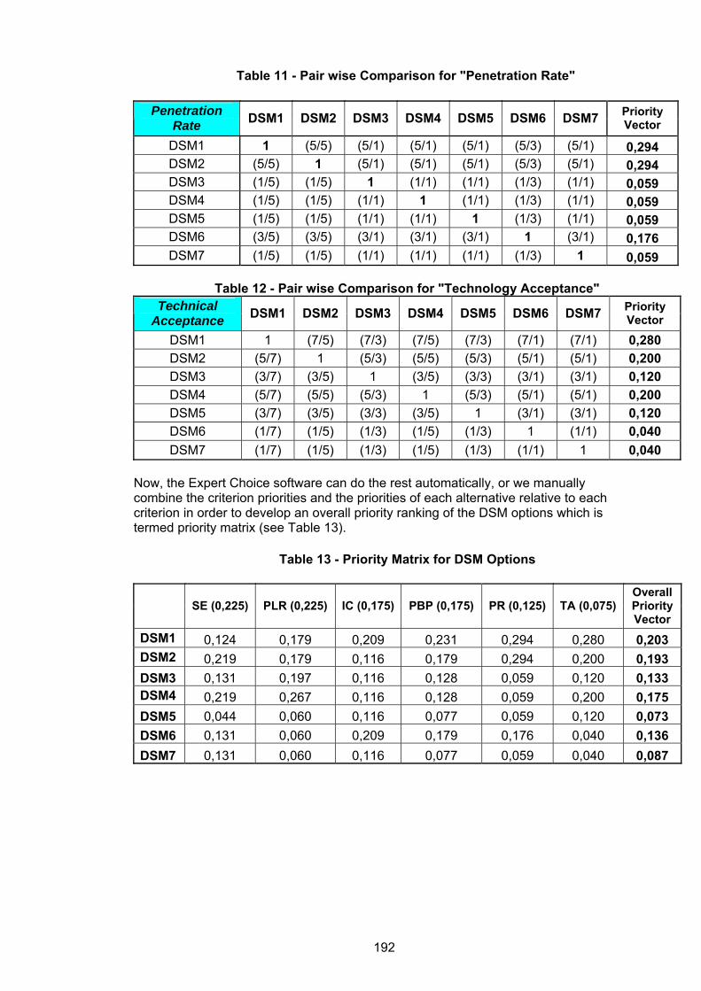
192

Table 11 - Pair wise Comparison for "Penetration Rate"

Penetration Rate DSM1 DSM2 DSM3 DSM4 DSM5 DSM6 DSM7 Priority

Vector

DSM1 1 (5/5) (5/1) (5/1) (5/1) (5/3) (5/1) 0,294 DSM2 (5/5) 1 (5/1) (5/1) (5/1) (5/3) (5/1) 0,294 DSM3 (1/5) (1/5) 1 (1/1) (1/1) (1/3) (1/1) 0,059 DSM4 (1/5) (1/5) (1/1) 1 (1/1) (1/3) (1/1) 0,059 DSM5 (1/5) (1/5) (1/1) (1/1) 1 (1/3) (1/1) 0,059 DSM6 (3/5) (3/5) (3/1) (3/1) (3/1) 1 (3/1) 0,176 DSM7 (1/5) (1/5) (1/1) (1/1) (1/1) (1/3) 1 0,059

Table 12 - Pair wise Comparison for "Technology Acceptance"

Technical Acceptance DSM1 DSM2 DSM3 DSM4 DSM5 DSM6 DSM7 Priority

Vector DSM1 1 (7/5) (7/3) (7/5) (7/3) (7/1) (7/1) 0,280 DSM2 (5/7) 1 (5/3) (5/5) (5/3) (5/1) (5/1) 0,200 DSM3 (3/7) (3/5) 1 (3/5) (3/3) (3/1) (3/1) 0,120 DSM4 (5/7) (5/5) (5/3) 1 (5/3) (5/1) (5/1) 0,200 DSM5 (3/7) (3/5) (3/3) (3/5) 1 (3/1) (3/1) 0,120 DSM6 (1/7) (1/5) (1/3) (1/5) (1/3) 1 (1/1) 0,040 DSM7 (1/7) (1/5) (1/3) (1/5) (1/3) (1/1) 1 0,040

Now, the Expert Choice software can do the rest automatically, or we manually combine the criterion priorities and the priorities of each alternative relative to each criterion in order to develop an overall priority ranking of the DSM options which is termed priority matrix (see Table 13).

Table 13 - Priority Matrix for DSM Options

SE (0,225) PLR (0,225) IC (0,175) PBP (0,175) PR (0,125) TA (0,075)

Overall Priority Vector

DSM1 0,124 0,179 0,209 0,231 0,294 0,280 0,203 DSM2 0,219 0,179 0,116 0,179 0,294 0,200 0,193 DSM3 0,131 0,197 0,116 0,128 0,059 0,120 0,133 DSM4 0,219 0,267 0,116 0,128 0,059 0,200 0,175 DSM5 0,044 0,060 0,116 0,077 0,059 0,120 0,073 DSM6 0,131 0,060 0,209 0,179 0,176 0,040 0,136 DSM7 0,131 0,060 0,116 0,077 0,059 0,040 0,087

193

The calculations for finding the overall priority of DSM options are given below for illustration purposes. Overall priority of DSM1 = 0.225 (0.124) + 0.225 (0.179) + 0.175 (0.209) + 0.175 (0.231) + 0.125 (0.294) + 0.075 (0.280) = 0.203 The same sequence of calculations are carried out for the overall priority of DSM2, DSM3, DSM4, DSM5, DSM5 and DSM7, giving the values 0.193, 0.133, 0.175, 0.073, 0136 and 0.087. Concluding the above AHP calculations we come to the following overall priority order of identified DSM options: DSM1 (20.3%), DSM2 (19.3%), DSM4 (17.5%), DSM6 (13.6%), DSM3 (13.3%), DSM7 (8.7%) and DSM5 (7.3%). References: [1] Saaty TL, Analytic Hierarchy Process. New York: McGraw-Hill, 1980 [2] Saaty TL, Decision making for leaders. Belmont, California, 1985. [3] Saaty TL, How to make a decision: The Analytic Hierarchy Process, The EU Journal of Operational Research, North-Holland, 1990. [4] Saaty TL, Kearns KP, Analytical Planning the organization of systems. The analytic hierarchy process series, 1991, USA.

194

Appendix to Ch 8

Forecast of Private Dwellings

Dwelling Stock

Villas Apartments Traditional Houses Year Existing New Total Existing New Total Existing New Total

Grand Total

2006 104650 3983 108633 122666 0 122666 36500 1394 37894 269193 2007 108633 4468 113100 122666 4580 127246 37894 1394 39288 279635 2008 113100 2714 115815 127246 3512 130758 39288 330 39618 286191 2009 115815 2780 118594 130758 3609 134367 39618 333 39951 292912 2010 118594 2846 121441 134367 3709 138076 39951 336 40286 299803 2011 121441 2915 124355 138076 3811 141887 40286 338 40625 306867 2012 124355 2985 127340 141887 3916 145803 40625 341 40966 314108 2013 127340 3056 130396 145803 4024 149827 40966 344 41310 321533 2014 130396 3130 133525 149827 4135 153962 41310 347 41657 329145 2015 133525 3205 136730 153962 4249 158211 41657 350 42007 336948 2016 136730 3282 140012 158211 4367 162578 42007 353 42360 344949 2017 140012 3360 143372 162578 4487 167065 42360 356 42716 353153 2018 143372 3441 146813 167065 4611 171676 42716 359 43075 361563 2019 146813 3524 150336 171676 4738 176414 43075 362 43436 370187 2020 150336 3608 153944 176414 4869 181283 43436 365 43801 379029 1. Sharing by dwelling type is: 40% for villas, 46% for flats, and 14% for traditional houses. 2. Sharing by dwelling type is: 40% for villas, 46% for flats, and 14% for traditional houses.

195

Appendix 8.1

Electricity Demand Forecast in Kuwait (Baseline Scenario)

Year Population

Installed Capacity

(MW)

Peak Load (MW)

Generated Energy (GWh)

Load Factor

(%)

Exported Energy1 (GWh)

Final Elec. Consumption2

(GWh)

Residential Sector (GWh)

Per Capita Consumption

(kWh) Max. Load Share

/ Capita (Watt)

2005 2244995 10189 8400 43734 59.43% 37906 33357 21682 16885 3742 2006 2328116 10229 8900 47605 61.06% 41570 36582 23778 17856 3823 2007 2410829 10655 9070 48761 61.37% 42422 37331 24265 17596 3762 2008 2498342 11082 9820 53476 62.16% 46524 40941 26612 18622 3931 2009 2589032 11736 10310 58011 64.23% 50470 44413 28869 19494 3982 2010 2683014 11914 10830 61660 64.99% 53644 47207 30684 19994 4037 2011 2780407 13914 11394 65829 65.95% 57271 50399 32759 20598 4098 2012 2881336 15414 11988 70529 67.16% 61360 53997 35098 21296 4161 2013 2985928 16316 12612 75565 68.40% 65742 57853 37604 22017 4224 2014 3094318 16838 13270 80960 69.65% 70435 61983 40289 22763 4289 2015 3206641 17377 13961 86741 70.93% 75465 66409 43166 23534 4354 2016 3323042 17933 14688 92934 72.23% 80853 71150 46248 24331 4420 2017 3443669 18507 15454 99570 73.55% 86626 76231 49550 25155 4488 2018 3568674 19099 16259 106679 74.90% 92811 81673 53088 26007 4556 2019 3698217 19710 17106 114296 76.27% 99437 87505 56878 26888 4625 2020 3832462 20341 17997 122457 77.67% 106537 93753 60939 27799 4696 AVG 68.12% Source: MEW, Statistical Year Book, 2006 (from 2005 to 2010, the rest by the author) 1. Exported energy = Generated energy - Consumption in power plants 2. Final energy consumption = Exported energy - Network T. & D. losses (12%)

196

Appendix 8.2

Forecast of Baseline End - Use Consumption of Selected Dwellings (Without any DSM Activities) (Low Baseline Scenario)

Annual Energy Stock (GWh) Villas Apartments Traditional Houses

Year Existing New Total Existing New Total Existing New Total

Grand Total

2005 - - 10777.8 - - 4126.5 - - 2608.8 17513 2006 10777.8 650.5 11428.3 4126.5 56.8 4183.4 2608.8 124.8 2733.7 18345 2007 11428.3 738.7 12167.0 4183.4 61.7 4245.1 2733.7 140.1 2873.7 19286 2008 12167.0 77.5 12244.5 4245.1 6.2 4251.2 2873.7 14.5 2888.2 19384 2009 12244.5 78.0 12322.5 4251.2 6.2 4257.4 2888.2 14.6 2902.8 19483 2010 12322.5 78.5 12401.0 4257.4 6.2 4263.6 2902.8 14.7 2917.5 19582 2011 12401.0 79.0 12480.0 4263.6 6.2 4269.8 2917.5 14.7 2932.2 19682 2012 12480.0 79.5 12559.4 4269.8 6.2 4276.0 2932.2 14.8 2947.0 19782 2013 12559.4 80.0 12639.4 4276.0 6.2 4282.2 2947.0 14.9 2961.9 19884 2014 12639.4 80.5 12720.0 4282.2 6.2 4288.4 2961.9 15.0 2976.8 19985 2015 12720.0 81.0 12801.0 4288.4 6.2 4294.7 2976.8 15.0 2991.9 20088 2016 12801.0 81.5 12882.5 4294.7 6.2 4300.9 2991.9 15.1 3007.0 20190 2017 12882.5 82.1 12964.6 4300.9 6.3 4307.2 3007.0 15.2 3022.2 20294 2018 12964.6 82.6 13047.2 4307.2 6.3 4313.4 3022.2 15.3 3037.4 20398 2019 13047.2 83.1 13130.3 4313.4 6.3 4319.7 3037.4 15.3 3052.8 20503 2020 13130.3 83.6 13213.9 4319.7 6.3 4326.0 3052.8 15.4 3068.2 20608 1. Sharing by dwelling type is: 40% for villas, 46% for flats, and 14% for traditional houses.

197

Appendix 8.3

Forecast of Baseline Dwellings Consumption (Without any DSM Activities) Annual Energy Stock (GWh) Villas Apartments Traditional Houses

Year Existing New Total Existing New Total Existing New Total

Grand Total

2005 - - 13879.9 - - 4983.6 - - 2856.0 21719 2006 13879.9 870.0 14749.9 4983.6 66.8 5050.4 2856.0 120.6 2976.6 22777 2007 14749.9 988.9 15738.8 5050.4 72.5 5122.9 2976.6 134.5 3111.1 23973 2008 15738.8 129.1 15867.9 5122.9 9.0 5131.9 3111.1 17.2 3128.3 24128 2009 15867.9 130.2 15998.0 5131.9 9.0 5140.9 3128.3 17.3 3145.6 24284 2010 15998.0 131.2 16129.3 5140.9 9.0 5149.9 3145.6 17.4 3162.9 24442 2011 16129.3 132.3 16261.6 5149.9 9.0 5158.9 3162.9 17.5 3180.4 24601 2012 16261.6 133.4 16395.0 5158.9 9.1 5168.0 3180.4 17.6 3198.0 24761 2013 16395.0 134.5 16529.5 5168.0 9.1 5177.1 3198.0 17.7 3215.7 24922 2014 16529.5 135.6 16665.1 5177.1 9.1 5186.2 3215.7 17.8 3233.5 25085 2015 16665.1 136.7 16801.8 5186.2 9.1 5195.3 3233.5 17.9 3251.3 25248 2016 16801.8 137.8 16939.6 5195.3 9.1 5204.4 3251.3 18.0 3269.3 25413 2017 16939.6 139.0 17078.6 5204.4 9.1 5213.5 3269.3 18.1 3287.4 25579 2018 17078.6 140.1 17218.7 5213.5 9.2 5222.7 3287.4 18.2 3305.5 25747 2019 17218.7 141.2 17359.9 5222.7 9.2 5231.8 3305.5 18.3 3323.8 25916

2020 17359.9 142.4 17502.3 5231.8 9.2 5241.0 3323.8 18.4 3342.2 26086

1.This Scenario of Baseline Consumption is based on the results of simulation

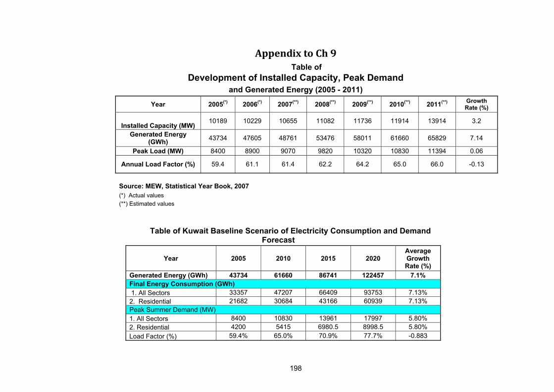
198

Appendix to Ch 9  Table of

Development of Installed Capacity, Peak Demand and Generated Energy (2005 - 2011)

Year 2005(*) 2006(*) 2007(**) 2008(**) 2009(**) 2010(**) 2011(**) Growth Rate (%)

Installed Capacity (MW) 10189 10229 10655 11082 11736 11914 13914 3.2

Generated Energy

(GWh) 43734 47605 48761 53476 58011 61660 65829 7.14

Peak Load (MW) 8400 8900 9070 9820 10320 10830 11394 0.06

Annual Load Factor (%) 59.4 61.1 61.4 62.2 64.2 65.0 66.0 -0.13

Source: MEW, Statistical Year Book, 2007 (*) Actual values (**) Estimated values

Table of Kuwait Baseline Scenario of Electricity Consumption and Demand Forecast

Year 2005 2010 2015 2020

Average Growth Rate (%)

Generated Energy (GWh) 43734 61660 86741 122457 7.1% Final Energy Consumption (GWh) 1. All Sectors 33357 47207 66409 93753 7.13% 2. Residential 21682 30684 43166 60939 7.13% Peak Summer Demand (MW) 1. All Sectors 8400 10830 13961 17997 5.80% 2. Residential 4200 5415 6980.5 8998.5 5.80% Load Factor (%) 59.4% 65.0% 70.9% 77.7% -0.883

199

Table of

DSM Impacts by Type of Dwelling - Annual Energy Savings (GWh)

Year Villas Apartments Tr. Houses Total % Residential % Final En. Consumption

2010 1671.1 530.8 326.3 2528.2 9.19% 5.36% 2011 1655.9 524.8 323.4 2504.1 8.69% 4.97% 2012 1677.9 529.2 327.4 2534.6 8.39% 4.69% 2013 1711.5 537.3 333.6 2582.3 8.16% 4.46% 2014 1751.0 547.9 341.2 2640.2 7.96% 4.26% 2015 1805.3 562.6 351.5 2719.5 7.82% 4.10% 2016 1880.3 584.0 366.0 2830.3 7.77% 3.98% 2017 1964.8 608.6 382.4 2955.9 7.74% 3.88% 2018 2062.0 636.9 401.3 3100.2 7.74% 3.80% 2019 2161.9 664.6 420.3 3246.8 7.74% 3.71% 2020 2232.1 681.6 433.0 3346.7 7.61% 3.57%

Total 20573.9 6408.5 4006.4 30988.8

200

Table of DSM Impacts by Type of Dwelling - Peak Demand Reductions (MW)

Year Villas Apartments Tr. Houses Total % Of Overall Peak Load

2010 245.4 85.0 49.0 379.4 3.5% 2011 243.6 84.2 49.1 376.8 3.3% 2012 263.8 91.2 53.7 408.7 3.4% 2013 292.5 101.4 60.2 454.2 3.6% 2014 327.1 113.9 68.4 509.4 3.8% 2015 374.6 131.1 79.4 585.1 4.2% 2016 440.6 155.2 94.9 690.6 4.7% 2017 519.1 184.1 113.6 816.8 5.3% 2018 614.3 219.1 136.4 969.8 6.0% 2019 720.2 257.8 161.8 1139.7 6.7% 2020 810.0 290.1 183.2 1283.4 7.1%

201

Table of Accumulated DSM Savings (2010 - 2020) Energy Savings (GWh)

Dwelling DSM1 DSM2 DSM3 DSM4 +

DSM7 DSM5 DSM6 Total Total with 0.8 D.F.

Villas 1102.8 1166 531.3 72.8 137.3 22737.2 25747.4 20598 Apartments 431.2 349.2 86.1 0.1 12.8 7131.1 8010.5 6408 Tr. Houses 213.4 256.6 74.9 1.2 15.2 4446.7 5008 4006

Total 1747.4 1771.8 692.3 74.1 165.3 34315 38765.9 31013

D.F. = Diversity Factor

Diversity Factor, where (a 0.8 diversity means that the device in question operates at its nominal or maximum load level 80% of the time that its connected and turned on).

202

Appendix to Ch 10

Program Participants for Traditional Houses

Dwellings Stock (Tr. Houses) Program Participants Year Existing New Total DSM1(*) DSM2(*) DSM3 DSM4(1) DSM5(2) DSM6(3) Total(4) % 2010 37543 2403 39946 781 781 781 481 781 4693 6638 16.62% 2011 39946 2557 42502 711 711 631 511 631 4993 6551 15.41% 2012 42502 2720 45223 842 842 714 544 714 5313 7174 15.86% 2013 45223 2894 48117 1076 1076 850 579 850 5653 8068 16.77% 2014 48117 3079 51196 1434 1434 953 616 953 6015 9123 17.82% 2015 51196 3277 54473 1935 1935 1167 655 1167 6400 10608 19.47% 2016 54473 3486 57959 2713 2713 1460 697 1460 6809 12681 21.88% 2017 57959 3709 61669 3698 3698 1785 742 1785 7245 15162 24.59% 2018 61669 3947 65615 4921 4921 2208 789 2208 7709 18205 27.74% 2019 65615 4199 69815 6220 6220 2808 840 2808 8202 21679 31.05% 2020 69815 4468 74283 7177 7177 3477 894 3477 8727 24742 33.31% Total 31508 31508 16834 7348 16834 71757 140631 (1) Applied only for new buildings (2) Combined with DSM7 (Labels and Standards) (3) With a minimum elasticity of -0.1, the reduction in energy consumption is 12,5%.and peak demand 2% (with tariff increase 125%)-Existing Dwellings Only

(4) A diversity factor 80% is considered in the summation

Saved E. 15.70% 16.60% 16.80% 24.20% 4.60% 12.50% Peak R. 12.60% 23.20% 16.40% 18.70% 2.91% 2.00%

203

Table 10.1 - Total Savings (Energy & Peak Demand) (2010 - 2019) By DSM Options and

Type of Dwelling Energy Savings (GWh) Peak Demand Reductions (MW)

DSM Option ID Villa Apartment

TR.

House Total Villa Apartment

TR.

House Total

Thermostat Resetting from 75

to 78 degree ºF. DSM1 857.0 256.0 165.0 1278.0 854.4 352.2 195.7 1402.3

Replacing Incandescent Bulbs

to CFL DSM2 906.0 271.0 174.0 1351.0 891.5 322.9 229.7 1444.1

Upgrade A/C Equipment to

Efficient Units with EER ≥ 11 DSM3 390.0 111.0 73.3 574.3 600.4 207.5 113.6 921.5

High Quality Wall and Roof

Insulation DSM4 66.0 4.4 8.6 79.0 322.7 0.0 4.6 327.3

Use Energy Efficient End-Use

Equipment (1) DSM5 107.0 30.2 20.1 157.3 99.2 16.0 9.1 124.3

Tariff Increase DSM6 20601.0 6477.0 4031.0 31109.0 253.8 100.5 65.0 419.3

Total 22927.0 7149.6 4472.0 34548.6 3022.0 999.1 617.6 4638.7

(1) Combined with DSM7 (Labels and Standards)