Demand Planning (DP) Supply Network Planning (SNP) and Deployment Production Planning and Detailed Scheduling (PP/DS

Part IV

Appendix

A

The Hitchhiker’s Guide to SAP APO

This appendix outlines the functionality and planning philosophy of SAPAPO beyond the SNP optimizer, the latter being the focus of the rest of thisbook. In this brief overview of what is in SAP APO we want to give a flavorof the rich functionality this tool has to offer without claiming to go intodetail which most probably would fill a number of additional books. We alsoomit system basis, architecture, and database considerations focusing on thebusiness application components. The purpose of this appendix is to give thereader a self-contained and quick reference to the SAP APO functionality.

Within the mySAP Business Suite, there is the supply chain managementoffering mySAP SCM providing solutions for supply chain collaboration, plan-ning, coordination, and execution processes. SAP APO is one component ofmySAP SCM providing functionality for planning and executing supply chainprocesses (cf. the official SAP documentation at http://help.sap.com/).

A.1 SAP APO Components

SAP APO itself consists of multiple components that are tightly integrated.In the literature the components are sometimes also called modules (cf. Dick-ersbach, 2004, [17]). The components differ in their level of planning detailand the respective time horizons. They can be arranged in the supply chainplanning matrix as demonstrated in Sect. 1.2 or be interpreted as constituentsof a hierarchical planning strategy. The components are

• Demand Planning (DP)• Supply Network Planning (SNP) and Deployment• Production Planning and Detailed Scheduling (PP/DS)• Transportation Management (Transportation Planning and Vehicle Schedul-

ing, TP/VS)• Global Available-to-Promise (Global ATP)

274 A The Hitchhiker’s Guide to SAP APO

Next to these there are the cross-functional components Supply Chain Collab-oration enabling data exchange with business partners using other systems orvia the internet and Supply Chain Monitoring providing supply chain perfor-mance KPIs, alerting in exception situations, and monitoring and comparingplan quality. There are also several industry-specific scenarios and functional-ity available, including a standard interface for connecting external optimizersto PP/DS for trim loss problems (cf. http://help.sap.com/).

A.2 Hierarchical Planning

SAP APO follows a hierarchical planning philosophy differentiating strategic,tactical, and operational planning. The different hierarchy levels are distin-guished by their planning horizon and the typical level of planning detail. Thecomponents listed above can nicely be associated with these three levels:

• Strategic planning: DP• Tactical planning: DP, SNP• Operational planning: DP, PP/DS, TP/VS, Global ATP

Demand Planning is listed in all three levels as it can hold long-term datasuch as sales forecasts as well as short-term data such as customer orders. Itis also a powerful tool to aggregate and manage data sourced from systemsexternal to SAP APO.

Below the domains of the individual components are outlined and someexamples for scenarios in which they work together are mentioned. Note thatthis description is not considered complete and depending on the specificbusiness processes of the SAP client there are numerous possibilities how toorchestrate the components of SAP APO and the ERP system.

DP is SAP APO’s demand management and operates on a data grid basedon time buckets and key figures. The time bucket lengths can be freely de-fined, e.g., the first weeks can be planned in daily buckets followed by weekly,monthly, and quarterly ones. Key figures hold different “types” of demanddata such as statistical forecast, customer demand, strategic sales targets,etc. In DP several sophisticated statistical methods are available to computeforecast data. Simulation scenarios allow what-if analyses, promotion planningand lifecycle planning are also part of DP. The data can be refined via collab-orative scenarios involving different departments within the company as wellas input from business partners with connected systems or via the internet(“collaborative demand planning”). An example for a DP scenario is com-bining the different forecast figures in the DP planning book (e.g., strategicand sales forecasts, customer data) to form a “consensus forecast” by freelydefinable macros. Forecast consumption allows defining requirement strate-gies that determine how to process customer orders and forecast values inthe same time bucket. An example is to consume sales forecast quantities byactual customer order volumes. DP can consider BOMs (DP PPMs/PDSs)

A.2 Hierarchical Planning 275

for determining component demand. Database-wise, DP uses InfoCubes, theSAP APO database, and liveCache.

Tactical planning is the domain of SNP performing mid-term supply chainplanning on discrete time buckets across all relevant locations and BOM-levels.Typically based on demand data that is released from DP, SNP uses an inte-grated supply chain model to calculate a sourcing, production, transportation,and distribution plan. Next to MILP-based optimization, which is the topicof this book, heuristics and constraint propagation algorithms are available tobe chosen to best meet the needs of the client. The algorithms are outlinedin Sects. 1.4.1–1.4.3. If it turns out the SNP plan cannot satisfy the require-ments forecasted by DP it might make sense to release the SNP plan to DP,adjust the forecast and re-iterate the SNP process with the new demand data.After production (i.e., after PP/DS, if all planning hierarchies are executed),deployment in SNP creates stock transfers and transport loads covering cus-tomer demand. Heuristics (applying fair-share rules if demand exceeds supplyor push rules if supply exceeds demand) and optimization are available as de-ployment algorithms. Database-wise, SNP uses the SAP APO database andliveCache.

New functionalities available in SAP APO release 5.0 relevant to optimiza-tion-based planning are the Explanation Tool and the Result Indicators (cf.http://help.sap.com/). Both are based on the optimization log data and digestthe data in the logs for easier interpretation by the user. The Explanation Toolfocuses on two typical supply chain exceptions: non-delivery of a demandand shortfall of safety stock. In order to provide a possible explanation itanalyzes the optimizer log analyzing the factors capacity constraints, time-based constraints and maximum lot sizes, product availability, lead time, andcosts. From the nature of an optimization model it can only come up with onepossible reason for each exception. Via configuration settings determining thesequence of the analysis several explanation targets can be met (e.g., checkfor maximum lot sizes before checking the cost structure, or vice versa). TheResult Indicators take data from the optimization logs, too, and present theuser with the quality of the solution expressed in terms of demand fulfillment,stock level, and resource utilization data.

PP/DS is targeted at short-term production planning and scheduling.Based on an SNP plan or directly on demand data from DP, PP/DS cre-ates a detailed production plan. Differing from the SNP concept the plan iscalculated in a time continuous way rather than being based on time bucketsand reflects the actual order sequence on the resource-level accurate to thesecond. The available planning algorithms are based on heuristics, constraintpropagation, and evolutionary algorithms. Integrating PP/DS with medium-term planning is highly customizable and works via different order types forSNP and PP/DS and planning horizons determining whether a specific de-mand or order is planned by SNP or PP/DS. If releasing demand data fromDP, for instance, those requirements inside the PP/DS horizon will be inPP/DS responsibility. Planned orders created by SNP and released to PP/DS

276 A The Hitchhiker’s Guide to SAP APO

are converted into PP/DS planned orders and scheduled in the next PP/DSrun. In a classical integration scenario with the execution system (in mostcases this will be SAP R/3) the planned orders created by PP/DS are imme-diately visible and executed in the ERP system. Next to heuristics there isthe “PP/DS optimizer” that uses constraint propagation and evolutionary al-gorithms. Database-wise, PP/DS uses the SAP APO database and liveCache.

Global ATP and Capable-to-Promise (CTP) provide functionality for oper-ational order promising. In order to match the specific business environment,configurable rules are applied to finding supply for an order (including, forexample, location and product substitution). If desired checks can be madeagainst available production capacity and orders can be scheduled to satisfythe demand by using CTP calling PP/DS for order scheduling or multi-levelATP (including BOM explosion). Global ATP can be configured such thatupon order entry in an connected SAP R/3 system SAP APO is called in thebackground and the confirmation dates show directly on the SAP R/3 orderentry screen. As sales order confirmation is a sequential process (first come,first served), it might be necessary to redistribute the confirmed quantitiesbased on priority rules. This is done by backorder processing, a functionalitythat can be seen as part of Global ATP in SAP APO. Database-wise, GlobalATP and CTP use the SAP APO database and liveCache.

Finally, there is TP/VS planning transportation. This is not to be con-fused with SNP that also considers transportation relationships between loca-tions and results in according planned stock transfers. In a two-step process,TP/VS consolidates freight units characterized by start and destination loca-tion, quantity, and date into shipments (defining mode of transportation androute) and then assigns transportation service providers to those shipments.This can be done manually or by applying evolutionary algorithms in the firststep and – starting with SAP APO release 5.0 – mixed integer optimizationin the second step. Database-wise, TP/VS uses the SAP APO database andliveCache.

B

Mathematical Foundations of Optimization

This appendix provides some of the mathematical foundations of optimiza-tion and provides the platform enabling the reader to understand the opti-mization algorithms embedded in SAP APO. This knowledge is valuable tojudge whether a standard approach is technically sufficient to tackle a chal-lenging problem or whether individual solution approaches are necessary andpromising. Linear programming (LP) is a well established approach. Problemswith millions of variables can be solved by standard solvers. Larger problemscan be solved by special approaches such as column generations techniques.Mixed integer linear programming (MILP) problems involving thousands ofbinary and integer variables can be solved using commercial branch-and-bound solvers. Presolving techniques are very elaborated. Advanced branch-and-cut and branch-and-price methods coupled to column generation methodsare available to solve even larger problems.

B.1 Linear Programming

Consider the linear optimization problem (often called: linear program) instandard form1

LP : max{

cTx | Ax = b, x ≥ 0, x ∈ IRn, b ∈ IRm}

(B.1)

where IRn denotes the vector space of real vectors with n components and Ais a m × n matrix.

Commercial software for solving linear programing problems usually pro-vides two alternative solution approaches: vertex-based methods such asSimplex-algorithms, and interior point methods.

One of the best known algorithms for solving LPs is the simplex algorithmdeveloped by George B. Dantzig in 1947 and described in Dantzig (1963, [15])

1 LP problems with upper bounds are discussed in Appendix B.1.3.

278 B Mathematical Foundations of Optimization

or, e.g., Padberg (1996, [76]). The first step is to compute an initial feasiblesolution [see Section B.1.2] as a starting point, possibly by using another LPmodel which is a variant of the original model but allows us easily to deter-mine an initial feasible solution. The simplex or the revised simplex (a morepractical and efficient form for computer implementation) algorithm finds anoptimal solution of an LP problem after a finite number of iterations, but inthe worst case the running time may grow exponentially, i.e., for large prob-lems we should be prepared that running time is an exponential function of thenumber of variables and constraints. Nevertheless on many real-world prob-lems it performs better than so-called polynomial time algorithms developedin the 1980s, e.g., by Karmarkar (1984, [56]).

In most commercially available software systems the simplex algorithmprovides the foundation of a method which will comfortably produce rapidsolutions to problems involving 1,000,000s of variables and 100,000s of con-straints. When a problem is formulated as an LP, the formulation will not beunique, e.g., some modelers may prefer to introduce certain variables to repre-sent intermediate stages in operations while others will avoid these concepts.However, provided the models are valid representations of the problem thenthe resulting LP problems will all be essentially equally easy to solve and willprovide equivalent solutions.

In contrast to the idea of a vertex-following method to solve an LP prob-lem, more recently developed methods have concentrated on moving throughthe interior of the feasible region, a polyhedron in linear programming prob-lems. Such methods are called interior-point methods and first received wide-spread attention after work by Karmarkar (1984, [56]). Since then, about 2000papers have been written on the subject and research in optimization experi-enced the largest boom since the development of the simplex method (Freundand Mizuno, 1996, [27]). The idea of interior-point methods is intuitively sim-ple if we take a naive geometric view of the problem. However, first, it shouldbe noted that in fact the optimal solution to an LP problem will always lieon a vertex, i.e., on an extreme point of the boundary of the feasible region.Secondly the shape of the feasible region is not like, say, a multi-faceted pre-cious stone stretched out equally into many dimensions but more likely toresemble a very thin pencil stretched out into many dimensions. Hence, analgorithm which moves through the interior of a region must pay attention tothe fact that it does not leave the feasible region. Approaching the boundaryof the feasible region is penalized. The penalty is dynamically decreased in or-der to find a solution on the boundary. Interior-point methods will in generalreturn an approximately optimal solution which is strictly in the interior ofthe feasible region. Unlike the simplex algorithm no optimal basic solution isproduced. Thus, “purification” pivoting procedures from an interior point to avertex having an objective value no worse have been proposed and cross-overschemes to switch from interior-point algorithm to the simplex method havebeen developed [2].

B.1 Linear Programming 279

B.1.1 A Primal Simplex Algorithm

For an elementary treatment and examples for the primal simplex algorithmsee Kallrath & Wilson (1997, [55, Chap. 3 and Appendix]) and Kallrath (2002,[51]). Here, we just summarize the abstract ideas and consider the linearprogram (B.1). Vertex-based methods, the Simplex-algorithm is a special case,exploit the concept of basic variables collected into the basic vector xB . Thealgebraic platform is the concept of the basis B of A, i.e., a linearly independentcollection B = {Aj1 , ...,Ajm} of columns of A. Sometimes, just the set ofindices J = {j1, ..., jm} referring to the basic variables or linearly independentcolumns of A is referred to as the basis. The inverse B−1 gives a basic solutionx ∈ IRn which is given by

xT=(xT

B ,xTN

)where xB is a vector containing the basic variables computed according to

xB = B−1b

and xN is an (n − m)-dimensional vector containing the non-basic variables:

xN = 0 , xN ∈ IRn−m

If x is in the set of feasible points S = {x : Ax = b, x ≥ 0} , then x is calleda basic feasible solution or basic feasible point . If

1. the matrix A has m linearly independent columns Aj ,2. the set S is not empty and3. the set {cTx : x ∈ S} is bounded from above,

then the set S defines a convex polyhedron P and each basic feasible solutioncorresponds to a vertex of P . Assumptions (2) and (3) ensure that the LP isneither infeasible nor unbounded, i.e., it has a finite optimum.

It can be shown that in order to find the optimal solution it is sufficientto consider all basic solutions (sets of m linearly independent columns of A),check whether they are feasible, compute the associated objective function,and pick out the best one. In this sense finding an optimal solution for anLP is a combinatorial problem. An LP problem can have at most m positivevariables in the solution. At least n − m variables, these are the non-basicvariables, must take the value zero. McMullen (1970, [68]) has shown thatthere can exist at most2

f(n, m) :=(

n −⌊

m+12

⌋n − m

)+

(n −

⌊m+2

2

⌋n − m

)(B.2)

basic feasible solutions. Therefore, this purely combinatorial approach is notattractive in practice.2 This result is only true if no upper bounds [see Section B.1.3] are present.


Geometrically the (primal) simplex algorithm can be understood as anedge-following algorithm that moves on the boundary of a polyhedron repre-senting the feasible set, i.e., from vertex to vertex of the polyhedron. In eachmove corresponding to a linear algebra step (technically, a Pivot step) theobjective function value is either improved or does not change. Algebraically,in each iteration, one column of the current basis is modified, according to thisexchange of basic variables, matrix A, and vectors b and c are transformed tomatrix A′, and vectors b′ and c′. Technically, this procedure is called a pivotor pivot operation or pivot step.

Now we can also understand degenerate cases in LP. A purely algebraicconcept is to call an LP problem degenerate if the optimal solution containsbasic variables with value zero. If we combine the algebraic and geometricaspects we can interpret a degenerate problem as one in which a certain vertex(usually we are considering the one leading to optimal objective function) hasdifferent algebraic representations, i.e., two vertices are co-incident with anedge of zero length between them.

Instead of keeping and computing the complete matrix A based on theprevious iteration, the revised simplex algorithm is based on the initial dataA,b and cT, and on the current basis inverse B−1.

The first step is to find a feasible basis B as described in Section B.1.2.Note that this problem is, in theory, as difficult as solving the optimizationproblem itself.

Once the basis is known we can compute3 the inverse, B−1, of the basis,the values of the basic variables

xB = B−1b (B.3)

and the dual values, πT,πT := cT

BB−1 (B.4)

Note that πT is a row vector. Now we are in the position to compute thereduced costs, dj ,

dj = cj − πTAj (B.5)

for the non-basic variables [the reduced cost of the basic variables are all equalto zero d(xB) = 0]. Note that formula (B.5) computes the reduced costs byusing only the original4 data cj and Aj , and the current basis B. If any ofthe dj are positive, we can improve the objective function by increasing thecorresponding xj . So, the problem is not optimal. The choice of which positivedj to select is partly heuristic: conventionally, one chooses the largest dj butcommercial solvers are different from textbook implementations. They useso-called partial pricing and also devex pricing [36]. The term partial pricing

3 As further pointed out on page 282 the basis inverse is only rarely inverted ex-plicitly.

4 From now on Aj denotes the columns of the original matrix A corresponding tothe variable xj .


indicates that the reduced costs are not computed for all non-basic variables.Sometimes, the first reduced cost with positive5 sign gives the variable tobecome the new basic variable. Other heuristics choose one of the non-basicvariables with positive sign randomly. And there must be a heuristic devicewhich tells the algorithm when to switch from partial to full pricing. Onlyfull pricing can do the optimality test. A sufficient optimality criterion for anoptimal solution of a maximization problem is

dj = cj − πTAj ≤ 0 , ∀j (B.6)

In a minimization problem the criterion is

dj = cj − πTAj ≥ 0 , ∀j

Note that we said a sufficient but not necessary condition. The reason is that inthe case of degeneracy several bases define the same basic feasible solution andsome can violate the criterion. If nondegenerate, alternative optimal solutionsexist (this case is called dual degeneracy) then necessarily the reduced cost forsome of the non-basic variables are equal to zero. If dj < 0 for all non-basicvariables in a maximization problem then the optimal solution is unique.

If we have not yet reached optimality we check whether the problem isunbounded. If the problem is bounded we use the minimum ratio rule toeliminate a basic variable. Both steps are actually performed simultaneously:the minimum ratio rule fails precisely when the incoming vector gives infiniteimprovement. The data needed for applying the minimum ratio rule are alsoderived directly from B−1

A′j = B−1Aj

After the minimum ratio rule has been applied we have the new basis, i.e., aset of indices or linearly independent columns.

What needs to be done is to get the current basis inverse B−1. There areseveral formulae to do this, but all of them are equivalent to computing thenew basis inverse although the inverse is never computed explicitly. To becorrect, the basis is only rarely inverted explicitly. Elementary row operationscarry over the existing basis inverse to the next iteration.6 However, every,say 100 iterations, the basis inverse is refreshed by inverting the basis matrix5 In this case we are solving a maximization problem.6 If we inspect the system of linear equations in each iteration we see that columns

associated with the original basic variables give the basis inverse associated withthe current basis. The reason is that elementary row operations are equivalentto a multiplication of the matrix representing the equations by another matrix,say M. If we inspect the first iteration we can understand how the method works.The initial matrix, and in particular the columns corresponding to the new basicvariables are multiplied by M and obviously give B·M = 1l, where 1l is the unitmatrix. Thus we have M = B−1. Since we have multiplied all columns of A by M,and in particular also the unit matrix associated with the original basic variables,these columns just give the columns of the basis inverse B−1. In each iteration k


taken from the original matrix A. Through this procedure, rounding errors donot accumulate. In addition, in most practical applications A is very sparsewhereas after several iterations the transformed matrix A′ becomes denserso that, especially for large problems, the revised simplex algorithm usuallyneeds far less operations.

The algorithm continues by computing the values of the basic variables,dual values, and so on until optimality is detected.

Let us come back to the basis inverse. Modern software implementationsof the revised simplex algorithms do not calculate B−1 explicitly. Insteadcommercial software uses the product form

Bk = B0η1η2 . . . ηk

of the basis to express the basis after k iteration as a function of the initialbasis B0 (usually a unit matrix) and the so-called rather the eta-matrices oreta-factors ηi. The ηi-matrices are m × m matrices

η = 1l + uvT

derived from the dyadic product of two vectors u and v leading to a verysimple structure (“1” on the diagonal, and just non-zeros in one column). Tostore the η-matrices it is sufficient to store the η-vectors u and v. Computingequations such as BxB = b yielding xB = B−1b are then solved by

xB = η−1k η−1

k−1 . . . η−11 b

The inverse of the η-matrices (under appropriate assumptions) can be com-puted very easily according to the formula

η−1 = 1l − 11 + vT u

uvT

Note that we need to store all ηi-vectors. As the iterations proceed, the amountof storage for the factors increases. So a re-inversion of the basis occurs notonly for reasons of numerical accuracy but also due to a “storage versus com-putation” trade off. Readers more interested in the details of the linear algebracomputations, LU factorizations, η-vectors and conserving sparsity may ben-efit from reading Gill et al. (1981, [29], p.192), Padberg (1996, [76, Sect. 5.4])and Vanderbei (1996, [97]).

An important idea in LP is the dual problem and its corresponding primalproblem (the original problem). When the dual problem is solved, the optimalvalues of its variables (and slacks) correspond to the values of the reduced costsand shadow prices of the primal problem. Thus the operation of the simplexalgorithm on the primal problem is governed by the updating of the solution

we multiply our original matrix by such a matrix Mk, so the orginal basic columnsrepresent the product of all matrices Mk which then is the basis inverse of thecurrent matrix.


values of the dual problem which provides current values of the reduced costson variables. Thus the simplex algorithm is an algorithm which is implicitlymoving between the primal and dual problems, updating solution and reducedcost values respectively.

Understanding the concept of dual values and shadow prices we can alsogive another interpretation of the reduced costs in terms of shadow prices.While the dual values, or Lagrangian multipliers, give the cost for activeconstraints, the reduced cost of a non-basic variable is the shadow price formoving it away from zero, or, in the presence of bounds on the variable,to move the non-basic variable fixed to one of its bounds away from thatbound. That also explains why basic variables have zero reduced costs: innon-degenerate cases, basic variables are not at their bounds.

B.1.2 Computing Initial Feasible LP Solutions

The simplex algorithm explained so far always starts with an initial feasiblebasis and iterates it to optimality. We have not yet said how we could providean initial solution. There are several methods, but the best known are bigM methods and phase I and phase II approaches. Less familiar are heuristicmethods usually referred to as crash methods. To discuss the first two methodsconsider the LP problem with n variables and m constraints in standard form[here it is advantageous to consider a minimization problem]

min cTx

subject toAx = b , x ≥ 0

By multiplying the equations Ax = b by −1 where necessary we can assumethat b ≥ 0. That enables us to introduce non-negative violation variables v =(v1, . . . , vm) and to modify the original problem to

min cTx + M

m∑j=1

vj

subject toAx + v = b , x ≥ 0 , v ≥ 0

M is a “big” number, say 105, but it is very problem dependent as to whatbig means. The idea of the big-M method is as follows. It is easy to find aninitial feasible solution. Can you see this? Check that

v = b , x = 0

is an initial feasible solution. Now we are able to start the simplex algorithm.If we choose M to be sufficiently large, we hope that we get a solution inwhich none of our violation variables is basic, i.e., v = 0. What if we find a


solution with some positive variables vj? In that case either M was too small,or our original problem is infeasible. How do we know the right size of M?One could start with small values, and check whether all violation variablesare zero. If not, one increases M . Ultimately, M must become very large if theproblem appears infeasible and one is essentially doing the two-phase methoddescribed in the next paragraph.

There is an alternative approach which does not depend on a scaling pa-rameter such as M : the two-phase method. The idea is the same but it usesa different objective function, namely

minm∑

j=1

vj

i.e., just the sum of the violation variables. Non-zero objective function valuesprove that the original problem is infeasible.

Why do we have two methods? Would not one be enough? If you inspectboth methods carefully you will notice that they have different advantages ordisadvantages. If one takes the limit M → ∞ the big M methods becomesthe two-phase method. Using the big M method the software designer has toensure and to worry that M is big enough. Often M is adapted dynamicallywhen trying to find an initial solution. It is just good enough to find a solutionwith v = 0. Keeping the original variables in the objective function mayprovide an initial solution which is closer to the optimal solution. In practicethe number of artificial variables is kept to a minimum. If a certain row alreadyhas a slack or surplus variable there is no need to introduce an additional one.Mixtures of big M and two-phase methods are also used.

In addition, commercial LP software employs so-called crash methods.These are heuristic methods aiming at finding an extremely good initial solu-tion very close to the optimal solution.

Initial feasible LP solutions can also be computed by re-using a basis savedfrom a previous related run. This approach produces good initial feasiblesolutions quickly if the model data have only changed a bit, or if only a fewvariables or constraints have been added.

New methods for computing initial solutions or good starting candidatesare hybrid methods. Such methods, combining the simplex algorithm andinterior-point method, are described in the Section B.1.5.

B.1.3 LP Problems with Upper Bounds

So far we have considered the LP problem with n variables and m constraintsin standard form [it is not really important whether we consider a minimiza-tion or maximization problem]

min cTx

subject to


Ax = b , x ≥ 0

In many large real-world problems it is advantageous to exploit another struc-ture which occurs frequently, upper and lower bounds on the variables. Thisis formulated as

min cTx′

subject toAx′ = b′ , l′≤ x′≤ u′

Since we always can perform a variable substitution x = x′−l′ and observingthat the new variables have the bounds 0 ≤ x ≤ u′−l′ = u, it is sufficient toconsider the problem

min cTx

subject toAx = b , 0 ≤ x ≤ u

Of course we could reformulate this problem by introducing some slack vari-ables s ≥ 0 in the standard way

min cTx

subject toAx = b

x + s = u , x ≥ 0 , s ≥ 0

Since in many large real-world problems we have n � m (there are oftenbetween three and ten times as many variables as rows) a straightforwardapplication of the simplex algorithm would lead to a very large basis of size(m+n)× (m+n). Exploiting the presence of the upper bounds will lead to amodified simplex algorithm which still is based on a basis of size m×m only.

The idea is to distinguish between nonbasic variables, xj , j ∈ J0, thatare at their lower bound of zero (the concept we are familiar with) and thosexj , j ∈ Ju, that are at their upper bound (the new concept). With the newconcept no explicit slack variables are necessary. Let us now try to see how thesimplex algorithm works when performing a basis exchange. Pricing now tellsus that a current basis is not optimal if one of these two situations occurs:

1) there exist indices j ∈ J0 with dj < 02) there exist indices j ∈ Ju with dj > 0

In case 1) we could increase a nonbasic variable, in case 2) we could decreaseit. Both cases would lead to a decreased value of the objective function. A newconsideration, when increasing or decreasing a nonbasic variable, is that weneed to calculate whether it could reach its upper (respectively lower) bound.

The minimum ratio rule controls how we could change a nonbasic variable.We have to stop increasing a nonbasic variable when one of the basic variablesbecomes zero. The minimum ratio rule in the presence of upper bounds on


variables gets a little bit more complicated since variables might hit theirupper bounds.

Case 1) leads to two sub-cases:

1a) the nonbasic variable xj can be increased to its upper bound while nobasic variables reaches zero or its upper bound, or

1b) while increasing the nonbasic variable xj a basic variable reaches zero,or a basic variable reaches its upper bound.

Case 1a), called a flip for obvious reasons, is easy to handle: one just movesthe index j into the new set Ju. Reaching zero in 1b) is handled as in thestandard simplex algorithm: variable xj enters the basis and the index of thevariable leaving the basis is added to the new set J0. When an upper bound ishit in 1b) the variable xj enters the basis and the index of the variable leavingthe basis is added to the new set Ju.

Case 2) can be analyzed by considering the slack sj = uj − xj . If thenonbasic variable xj is at its upper bound then sj is at its lower bound (zero).sj plays the same role (note that its upper bound is uj) as the nonbasicvariable xj considered in 1a) and 1b) and thus the argument is the same.

The linear algebra involved in the iteration is similar to the standardsimplex, and essentially no extra computations are required. Readers moreinterested in the subject are referred to Padberg (1996, [76, pp.75-80]).

We have now seen why exploiting bounds on variables explicitly leadsto better, i.e., faster numerical, performance: there is a little more testingand logic required in the algorithm but no additional computations. This hassignificant consequences for the B&B algorithm which adds only new boundsto the existing problem.

Note that since the bounds are treated explicitly and not as constraints noshadow prices are available on these “constraints”. Instead, the shadow pricescan be derived from the reduced costs of the nonbasic variables fixed at theirupper bounds.

B.1.4 Dual Simplex Algorithm

The (primal) simplex algorithm concentrates on improving the objective func-tion value of an existing basic feasible solution. In contrast, there is also thedual simplex algorithm which solves an LP problem by taking a dual optimalbasic solution which is optimal in the sense that the reduced costs computedaccording to (B.5) have the correct sign, but are not basic feasible. The dualsimplex algorithm tries to achieve feasibility of the solution while retaining itsoptimal properties. The two approaches can be seen as “dual” to each other:while the primal algorithm makes the choice of the new basic variable first,and then decides on which existing basic variable should be eliminated, thedual algorithm eliminates first an existing basic variable, and then selects anew basic variable.


The dual simplex algorithm is often used within the B&B algorithm. Whena branch is made the subproblem just differs from the original problem inhaving a different bound on the branching variable; remember from SectionB.1.3 that bounds can be treated very efficiently in the simplex algorithm.So the LP solution obtained at the parent node could now be consideredoptimal but not feasible. In most cases, the dual simplex algorithm restoresfeasibility quickly to the solution, say, within a few iterations. By using thedual simplex algorithm we are able to take advantage of the earlier work doneby the simplex algorithm and then move to a new optimal solution quickly.However, there is no guarantee that this will always happen. If the (primal)simplex algorithm was used after each branch the problem would need to besolved from the start again and this would be burdensome.

B.1.5 Interior-point Methods

In linear programming, interior-point methods (IPMs) are well suited espe-cially for large, sparse problems or those, which are highly degenerate. Hereconsiderable computing-time gains can be achieved. Such methods have al-ready been integrated into some LP-solvers, such as CPLEX or Xpress-MP.

The idea of IPMs is to proceed from an initial interior point x ∈ S satis-fying x > 0, towards an optimal solution without touching the boundary ofthe feasible set S. The condition x > 0 is (in the second and third method)guaranteed by adding a penalty term to the objective function.

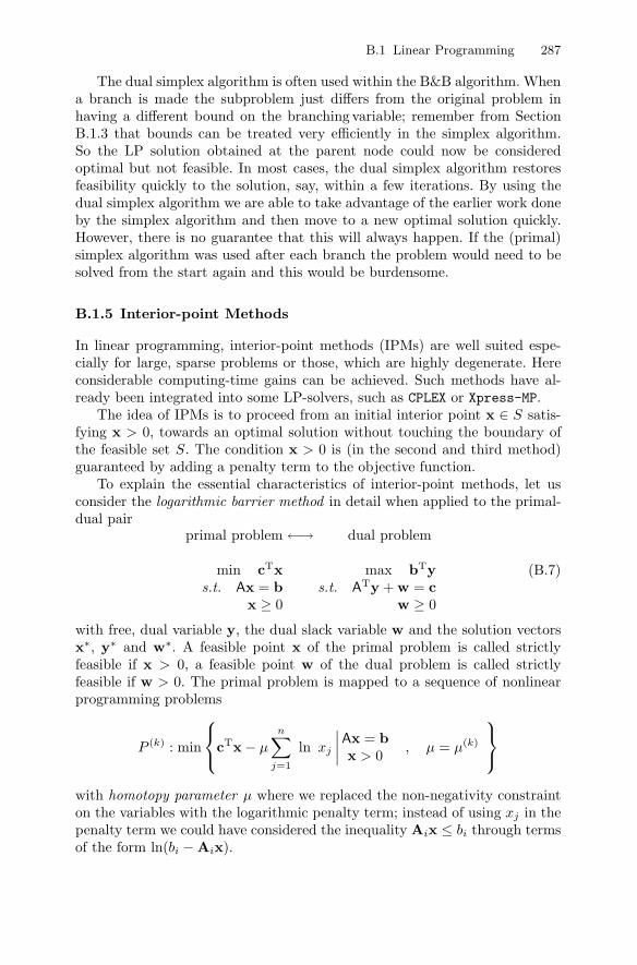
To explain the essential characteristics of interior-point methods, let usconsider the logarithmic barrier method in detail when applied to the primal-dual pair

primal problem ←→ dual problem

min cTx max bTys.t. Ax = b s.t. ATy + w = c

x ≥ 0 w ≥ 0

(B.7)

with free, dual variable y, the dual slack variable w and the solution vectorsx∗, y∗ and w∗. A feasible point x of the primal problem is called strictlyfeasible if x > 0, a feasible point w of the dual problem is called strictlyfeasible if w > 0. The primal problem is mapped to a sequence of nonlinearprogramming problems

P (k) : min

⎧⎨⎩cTx − µ

n∑j=1

ln xj

∣∣∣∣Ax = bx > 0 , µ = µ(k)

⎫⎬⎭

with homotopy parameter µ where we replaced the non-negativity constrainton the variables with the logarithmic penalty term; instead of using xj in thepenalty term we could have considered the inequality Aix ≤ bi through termsof the form ln(bi − Aix).


At every iteration step k, µ is newly chosen as described, for instance, in[55, Chap. 3 and Appendix]. The penalty term, and therefore the objectivefunction, increases to infinity. By suitable reduction of the parameter µ > 0,the weight of the penalty term, which gives the name logarithmic barrierproblem to this methods, is successively reduced and the sequence of pointsobtained by solving the perturbed problems, converges to the optimal solutionof the original problem. So, through the choice of µ(k) a sequence P (k) ofminimization problems is constructed, where the relation

limk→∞

µ(k)n∑

j=1

ln xj = 0

has to be valid, viz.

limk→∞

argmin(P (k)) = argmin(LP ) = x∗

where the function argmin returns an optimal solution vector of the problem.We have replaced one optimization problem, namely (B.7), by several more

complex NLP problems. So, it is not a surprise to learn that interior-pointmethods are special homotopy algorithms for the solution of general non-linear constrained optimization problems. Applying the Karush-Kuhn-Tucker(KKT) conditions [Karush (1939, [57]) and Kuhn and Tucker (1951, [62])],these are the necessary or the sufficient conditions for the existence of localoptima in NLP problems, we get a system of nonlinear equations which can besolved with the Newton-Raphson algorithm as shown below. The good news isthat the problems P (k) or systems of nonlinear equations they produce neednot to be solved exactly in practice, but one is satisfied with the solutionachieved after one single iteration in the Newton-Raphson algorithm.

So far we have considered the primal problem. To get to the dual and finallythe primal-dual7 version of interior-point solvers used in commercial solvers,the Karush-Kuhn-Tucker (KKT) conditions are derived from the Lagrangianfunction (a common concept in NLP)

L = L(x,y) = cTx − µn∑

j=1

ln xj − yT(Ax − b) (B.8)

Note that the constraints are multiplied by the dual value (Lagrange multipli-ers), yT, and then are added to the original primal objective function. Detailsare provided, for instance, in [55, Chap. 3 and Appendix].

By definition interior-point methods operate within the interior of thefeasible region and thus need strictly positive initial guesses for the vectorsx and w. How can such feasible points be obtained? This is a very difficult7 The reason for using this expression is that the method will include both the

primal and dual variables.


task. The method described in Section B.1.2 does not help this time sincewe do not want to use the simplex algorithm. Since interior-point methodsare path-following methods one would like to have an initial point as close aspossible to the central path and to be as close to primal and dual feasibilityas possible. So called “primal-dual infeasible-interior-point methods” provedto be successful. These methods start with initial points x(0) and w(0) but donot require that primal and dual feasibility is satisfied. This is quite typical fornonlinear problems which use Newton type algorithms. Feasibility is attainedduring the process as optimality is approached8. Therefore, a primal and dualfeasibility test is part of the termination criterion; see, for instance, [55, Chap.3 and Appendix] for details.

Interior-point methods produce an approximation to the optimal solutionof an LP but no optimal basic and non-basic partition of the variables. Sincethe optimal solution produced by the interior-point method is strictly in theinterior of the feasible solution there are many more variables not fixed attheir bounds than we would expect in a simplex solution. The concept ofbasic solutions is, however, very important for sensitivity analyses and theuse of LP problems as subproblems in B&B algorithms. The availability of abasis facilitates warm-starts.

Commercial implementations of interior-point methods use cross-overtechniques, i.e., at some time controlled by a termination criterion the al-gorithm switches from the interior-point method to the simplex algorithm.Crossing-over starts with the basis identification providing a good feasibleinitial guess for the simplex algorithm to proceed. The simplex algorithmimproves this guess quickly and produces an optimal basic solution.

At the moment the best simplex algorithms and the best interior-pointmethods are comparable. The simplex algorithm needs many iterations, butthese are very fast. The number of the iterations grows approximately linearlywith the number of constraints and logarithmically in the number of variables.Interior-point methods usually need about 20 to 50 iterations; this numbergrows weakly with the problem size. Every iteration requires the solution ofan n × n system of nonlinear equations which is quite costly. This systemis linearized. Thus the central computing consumption for a problem with nvariables is the solution of a n × n linear equation system. That is why it isessential for the success of the IPM, that this system matrix is sparse.

Although problem dependence plays an essential role for the valuation ofthe efficiency of simplex algorithms and IPMs, the IPMs seem to have advan-tages for large, sparse problems. Especially for big systems hybrid algorithmsseem to be very efficient. In the first phase these determine a nearly optimalsolution with the help of an IPM, viz. determine a solution near the polyhe-8 The screen output of an interior-point solver may thus contain the number of the

current iteration, quantities measuring the violation of primal and dual feasibility,the values of the primal and the dual objective function (or the duality gap) andpossibly the barrier parameter as valuable information on each iteration.


dra edge. In the second phase, “purification” pivoting procedures are used tocreate a basis. Finally, the simplex algorithm uses this basis as an initial guessand finally iterates to the optimal basis. Further aspects of using the simplexalgorithm or IPMs are discussed, for instance, in [55, Chap. 3 and Appendix].

B.2 Mixed Integer Linear Programming

All commercial packages, in addition to more complicated methods, use vari-ants of the Branch and Bound (B&B) algorithm originally developed by Landand Doig (1960, [64]) to solve mixed integer linear programming problems.The B&B idea or implicit enumeration characterizes a wide class of algorithmswhich can be applied to discrete optimization in general. For an elementarytreatment see Kallrath & Wilson (1997, [55, Chap. 3 and Appendix]) andKallrath (2002, [51]). Here, we provide an orientation about this method andits relevant computational steps.

The branch in B&B hints at the partitioning process used to produceinteger feasible solutions or to prove the optimality of a solution. Lower andupper bounds are used during this process to avoid an exhaustive search inthe solution space. The algorithm terminates when the differences betweenupper and lower bounds becomes less or equal to a predefined value, ∆ ≥ 0(∆ = 0 for proving optimality).

The computational steps of the B&B algorithm are summarized as follows.After initialization the bounds and the nodes list, the LP-relaxation —thatis that LP problem obtained when relaxing all integer variables to contin-uous ones— establishes the first node. The node selection is obvious in thefirst step (just take the LP-relaxation), but later on it is based on variousheuristics. A B&B algorithm of Dakin (1965, [13]) with LP-relaxations usesthree pruning criteria: infeasibility, optimality and value dominance relation.In a maximization problem the integer solutions found lead to an increasingsequence of lower bounds, zIP, while the LP problems in the tree decrease theupper bound, zLP. Note that α denotes an addcut which causes the algorithmto accept a new integer solution only if it is better by at least the value of α.If the pruning criteria fail branching starts: the branching in this algorithmis done by variable dichotomy: for a fractional y∗

j two child nodes are createdwith the additional constraint yj ≤ [y∗

j ] resp. yj ≥ [y∗j ] + 1. Other possibili-

ties for dividing the search space are, for instance, generalized upper bounddichotomy or enumeration of all possible values, if the domain of a variableis finite ([8], [73]). The advantage of variable dichotomy is that only simplelower and upper bounds are added to the problem. In Section B.1.3 we haveshown why bounds can be treated much easier than general constraints.

The selection of nodes plays an important role in implicit enumeration;widely used is the depth-first plus backtracking rule as presented above. If anode is not pruned, one of its two sons is considered. If a node is pruned, the

B.2 Mixed Integer Linear Programming 291

algorithm goes back to the last node with a son which has not yet been con-sidered (backtracking). In linear programming only lower and upper boundsare added, and in most cases the dual simplex algorithm [see Section B.1.4]can reoptimize the problem directly without data transfer or basis re-inversion[73]. Experience has shown [8], that it is more likely that feasible solutionsare found deep in the tree. Nevertheless, in some cases the use of the oppositestrategy, breadth-first search, may be advantageous.

Another important point is the selection of the branching variable. A com-mon way of choosing a branching variable is by user-specified priorities, be-cause no robust general strategy is known. Degradations or penalties may alsobe used to choose the branching variables, both methods estimate or calcu-late the increase of the objective function value if a variable is required to beintegral, especially penalties are costly to compute in relation to the gainedinformation so that they are used quite rarely [73].

The B&B algorithm terminates after a finite number of steps. Termina-tion occurs when the lower and the upper bound cross or when the node listbecomes empty. In that case the result is either the optimal integer feasiblesolution or the message that the problem does not have any integer feasiblesolution. In practice, it happens very often that the user does not want towait until the node list becomes empty but wants to stop after one, or sev-eral integer solutions have been found. If an integer feasible solution has beenfound the upper and lower bounds mentioned above may be used to estimatethe quality of the solution. Let us see how that works: during the B&B for amaximization problem we know that

zLP ≥ z∗ ≥ zIP

where z∗ is the (unknown) value of the best integer solution, zIP (possibly−∞) is the value of the best integer solution found so far in the search andzLP = maxi{zLP

i } where zLPi is the optimal value of the LP-relaxation at

active node i (nodes that have been fathomed are not considered).The quality of the solutions is quantified by the integrality gap which is a

function of the upper and lower bounds derived by the B&B algorithm. In amaximization problem the upper bound, zU, is provided by the LP relaxationszLP while the lower bound, zL, corresponds to the best integer solution zIP

found. So we have the bounds

zL ≤ z∗ ≤ zU (B.1)

on the objective function value z∗ of the (unknown) optimal solution. In amaximization problem the difference zU − z∗ is called the integrality gap. Ifthe search is terminated before z∗ has been computed, the difference zU − zL

is used as an upper bound on the integrality gap.Assuming that both zL and zU are positive the quality of our solution can

also be expressed by the relative integrality gap

p := 100zU − zL

zL= 100

zLP − zIP

zIP(B.2)


which expresses that the difference between the best solution found and the(unknown) optimal solution is less than or equal to p% of the upper bound.With the present data, p is of the order of 10%.

While the lower bound zL increases if we allow the algorithm to seek forfurther integer feasible solutions the upper bound zU decreases very slowlyduring the computations. The upper bound can be decreased faster by usingthe Branch&Cut algorithm embedded by commercial MILP solvers.

The Branch&Bound algorithm terminates if zLP − zIP ≤ ∆, where ∆ issome tolerance. If ∆ = 0, we haven proven optimality. If ∆ > 0, we have founda solution which at most deviates by ∆ from the maximum z∗. So it can beseen that a criterion for node selection in B&B is to reduce the integrality gapzLP − zIP. One way to do this is to select a node which has a good chance ofyielding a new integer feasible solution better than the current zIP. Anotherway is to branch on the node having the largest zLP

i on the grounds thata descendant of this node will certainly have no higher a value of zLP

i , andprobably will have a lower value, in which case zLP will be smaller.

The interpretation of the percentage gap introduced above becomes diffi-cult if a model includes penalty terms containing weighting coefficients with-out any economic interpretation. Sometimes such penalty terms are used toreduce infeasibilties. To illustrate the problem let us consider the followingproblem with an objective function containing two penalty terms

min P1r1 + P2r2 (B.3)

where r1 and r2 are relaxation variables with the following meaning. The firstone, r1, measures the deviation from demand. The second one, r2, quantifiesthe deviation from a due time. A valuable and expensive material is rarelydemanded in fractional quantities, D, by important customers, but can beproduced only in kilograms; the amount produced is denoted by the integervariable π. Deviations from demand are not avoidable. It is allowed to produceless or more than the demand but the deviations should be kept at a minimum.Thus, r1 measures the deviation from the next integer values 1, 2 or 3, and soon. The relaxation or deviation variable r1 is related to π by the disjunctiveset9 of constraints

π + r1 = D ∨ π − r1 = D . (B.4)

The demand is subject to a due time, TD. The time at which the productionstarts is denoted by the variable tS.

tS + TP ≤ TD + r2 . (B.5)

Let us assume in this example that the processing time, TP, is one hour, i.e.,TP = 7. Further we assume that TD = 16 hours, i.e., the production shouldbe finished at 4pm. The personnel at the production floor tells us that the9 Kallrath & Wilson (1997, Sec. 6.2.3, [55]) outlines how to treat disjunctive sets

of constraints.

B.2 Mixed Integer Linear Programming 293

machine is not available before 10am. Therefore, whatever we do, the minimalvalue for r2 is r2 = 1 as tS ≥ 10. If we use an example value of D = 1.4 kg weobviously get the optimal value π = 1 and r1 = 0.4, and r2 = 1 as above.

The integrality gap for a minimization problem is defined as

p := 100zU − zL

zU= 100

zIP − zLP

zIP. (B.6)

The LP-relaxation gives π = 1.4, r1 = 0 and thus zLP = P2. If in the B&Balgorithm the node π ≥ 2 is evaluated first, the associated gap is

pπ≥2 = 100(0.6P1 + P2) − (0 + P2)

0.6P1 + P2= 100

0.6P1

0.6P1 + P2. (B.7)

Note that we have 0 ≤ pπ≥2 ≤ 100. If we increase P2 the gap pπ≥2 approacheszero. Thus, the gap depends significantly on scaling. The situation we arefacing here is, due to the appearance of r2 in (B.5), similar to adding a constantto the objective function. The lesson to be learned is that one needs to payattention to such issues. The penalty approach can be avoided completely byexploiting the goal programming approach outlined in Section 2.4.2.

The reader might have heard that MILP problems, and in particular,scheduling problems are hard problems and he might have learned that theyare classified as NP hard and in many cases NP complete. In complexitytheory these are measures of how difficult it is to solve a certain class of op-timization problems. It is important to treat problems with such attributesrespectfully. But it does not mean that they cannot be solved to optimality.It is just that they have bad scaling properties. If a standard method such asBranch&Bound works well for a given problem instance, one might experiencedifficulties if the problem size changes by even only 20%.

It is this complexity why we find that all commercial packages use pre-processing and presolving techniques to tighten the model at the root node orwithin the B&B algorithm. This pushes the limit of which problems can besolved continuously towards larger and larger problems.

Preprocessing methods introduce model changes to speed up the algo-rithms. The modifications are made, of course, in such a way that the feasibleregion of the MILP is not changed. They apply to both pure LP problemsand MILP problems but they are much more important for MILP problems.A selection of several preprocessing algorithms is found in Johnson et al.(1985, [47]). A more recent overview of simple and advanced preprocessingtechniques is given by Savelsbergh (1994, [83]). The reader is also referred tothe comprehensive survey of presolve10 methods by Andersen and Andersen10 The terms preprocessing and presolve are often used synonymously. Sometimes

the term presolve is used for those procedures which try to reduce the problem sizeand to discover whether the problem is unbounded or infeasible. Preprocessinginvolves the presolving phase but includes all other techniques which try, forinstance, to improve the MILP formulation.


(1995, [1]). Some common preprocessing methods are: presolve (arithmetictests on constraints and variables, bound tightening), disaggregation of con-straints, coefficient reduction, and clique and cover detection. Many of thesemethods are implemented in commercial software but vendors are usually notvery specific about which techniques they have implemented or methods used.In particular, during preprocessing constraints and variables are eliminated,variables and rows are driven to their upper and lower bounds, or an obvi-ous basis is identified. Being aware of these methods may greatly improvethe user’s model building leading to more efficient models or reduce the user’sefforts if it is known that the software already does certain presolve operations.

Commercial solvers, nowadays, also to apply heuristics to generate integerfeasible points from nodes still containing fractional values. These issues (pre-processing, presolve, constructive heuristics inside the B&B scheme) becomemore and more important in commercial MILP solver. They are the greatsecrets of the companies developing MILP solvers.

B.3 Multicriteria Optimization and Goal Programming

Here we provide examples illustrating two solution techniques for goal pro-gramming: the pre-emptive (lexicographic) and the Archimedian approach.

In pre-emptive goal programming goals are ordered according to impor-tance and priorities . The goals at a certain priority level are considered to beinfinitely11 more important than the goals in the next lower level. Pre-emptivegoal programming is recommended if there is a ranking between incommen-surate objectives available.

In the Archimedian approach weights or penalties are applied for notachieving targets. The following example illustrates this. Let

2x + 3y

represent profit, and

y + 8z

represent return on capital in a simple LP model where there are a number ofconstraints involving the variables x, y, and z and other variables. In addition,let P be the desired level of profit and C the desired level of return on capital.P and C might be obtained from last figures of last year plus some percentageto give targets for this year.

We now adjoin four non-negative variables d1, d2, d3, d4 ≥ 0 as well as twonew goal attainment constraints to our model11 It would also be possible to define weights which express how much the ith ob-

jective is more important than the (i + 1)th objective.

B.3 Multicriteria Optimization and Goal Programming 295

2x +3y +d1 − d2 = P goal 1y +8z +d3 − d4 = C goal 2

The objective function is to minimize deviation from target

min d1 + d2 + d3 + d4

Any objective function attempted previously in the formulation would haveto be expressed as a goal constraint. The problem is now an ordinary LPproblem. (IP problems may be modified similarly.) Note the use of two d’sin each constraint (with opposite signs) and the presence of all d’s in theobjective function (with the same sign). Note also how the d’s perform a roleto represent a free variable, namely the deviation from target. The techniquefor two goals can be extended to handle three or more goals.

One feature of goal programming is that every goal is treated as beingequally important, and consequently an excess of 100 units in one goal wouldbe compensated by a shortfall of 100 in another, or would be equivalent toexcesses of 10 units in each of 10 goals. Neither of these sets of circumstancesmight be desirable, so two strategies may be introduced:

(a) place upper limits on the values of d variables, e.g.,

d1 ≤ 10 , d2 ≤ 10 , d3 ≤ 5 , d4 ≤ 5

which will keep deviation from a goal within reasonable bounds;(b) in the objective function coefficients other than 1 may be used to

indicate the relative importance of goals. For example the objective

d1 + d2 + 10d3 + 10d4

may be considered appropriate if one can reason that a unit deviation inreturn is ten times as important as a unit deviation in “profit”.

Goals can be constructed from either constraints or objective functions(unconstrained N type rows). If constraints are used, the goals are to mini-mize the violation of the constraints. These are met when the constraints aresatisfied. In the pre-emptive case as many goals as possible are met in pri-ority order. (It should be remembered that someone has to subjectively setweights to achieve this.) In the Archimedian case a weighted sum of penaltiesis minimized. If the goals are constructed from an objective function rows,then in the pre-emptive case a target for each objective function row is calcu-lated from the optimal value for the objective function row (by percentage orabsolute deviation). In the Archimedian case a multi-objective LP problem isobtained, in which a weighted sum of the objective functions is minimized.

Let us illustrate how lexicographic goal programming works by consideringthe following example with two variables x and y subject to the constraint42x + 13y ≤ 100 as well as the trivial bounds x ≥ 0 and y ≥ 0. We are given


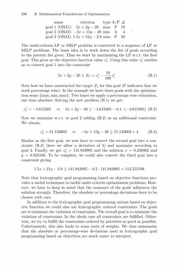
name criterion type A/P ∆goal 1 (OBJ1): 5x + 2y − 20 max P 10goal 2 (OBJ3): −3x + 15y − 48 min A 4goal 3 (OBJ2): 1.5x + 21y − 3.8 max P 20

.

The multi-criteria LP or MILP problem is converted to a sequence of LP orMILP problems. The basic idea is to work down the list of goals accordingto the priority list given. Thus we start by maximizing the LP w.r.t. the firstgoal. This gives us the objective function value z∗1 . Using this value z∗1 enablesus to convert goal 1 into the constraint

5x + 2y − 20 ≥ Z1 = z∗1 − 10100

z∗1 . (B.1)

Note how we have constructed the target Z1 for this goal (P indicates that wework percentage wise). In the example we have three goals with the optimiza-tion sense {max, min, max}. Two times we apply a percentage wise relaxation,one time absolute. Solving the new problem (B.1) we get:

z∗1 = −4.615385 ⇒ 5x + 2y − 20 ≥ −4.615385 − 0.1 · (−4.615385) (B.2)

Now we minimize w.r.t. to goal 2 adding (B.2) as an additional constraint.We obtain:

z∗2 = 51.133603 ⇒ −3x + 15y − 48 ≥ 51.133603 + 4 (B.3)

Similar as the first goal, we now have to convert the second goal into a con-straint (B.3) (here we allow a deviation of 4) and maximize according togoal 3. Finally, we get z∗3 = 141.943995 and the solution x = 0.238062 andy = 6.923186. To be complete, we could also convert the third goal into aconstraint giving

1.5x + 21y − 3.8 ≥ 141.943995 − 0.2 · 141.943995 = 113.555196

Note that lexicographic goal programming based on objective functions pro-vides a useful techniques to tackle multi-criteria optimization problems. How-ever, we have to keep in mind that the sequence of the goals influences thesolution strongly. Therefore, the absolute or percentage deviations have to bechosen with care.

In addition to the lexicographic goal programming variant based on objec-tive function we could also use lexicographic ordered constraints. The goalsare to minimize the violation of constraints. The overall goal is to minimize theviolation of constraints. In the ideals case all constraints are fulfilled. Other-wise, we try to fulfill the constraints ordered by priorities as good as possible.Unfortunately, this also leads to some sorts of weights. We thus summarizethat the absolute or percentage-wise deviations used in lexicographic goalprogramming based on objectives are much easier to interpret.

C

Glossary

The terms in this glossary are used in the text of the book and are defined herealso for the purpose of subsequent reference. Within this glossary all termswritten in boldface are explained in the glossary.

Algorithm: Probably derived from the name of the Arabian mathemati-cian al-Hwarizmı, a systematic procedure for solving a certain problem. Inmathematics and computer science it is required that this procedure can bedescribed by a finite number of unique, deterministic steps. At each step ofthe algorithm it is uniquely determined by the previous steps how to proceed.ATP: Available to promise; the business process describing the confirmationof sales orders. In software systems usually a set of rules exist that allow thesales representative to respond to customer inquiries with a delivery date. De-pending on the implementation and the software vendor, several variants exist:ATP looks at existing inventories and (planned) production orders, multi-levelATP considers rough-cut capacities and involves BOM explosion, and CTP(capable to promise) includes feasible scheduling of new production orders forfulfilling the new customer demand.Basic variables: Those variables in optimization problems whose values, innon-degenerate cases, are away from their bounds and are uniquely deter-mined from a system of equations.Basis (Basic feasible solution): In an LP problem with constraints Ax = band x ≥ 0 the set of m linearly independent columns of the m x n systemmatrix A of an LP problem with m constraints and n variables forming aregular matrix B. The vector xB = B−1b is called a basic solution. xB iscalled a basic feasible solution if xB ≥ 0.Bill of Material (BOM): A list of components that are used in producing amaterial. In case the components are procured the BOM is called single-level,otherwise the BOM is multi-level.

298 C Glossary

Bound: Bounds on variables are special constraints. A bound involves onlyone variable and a constant which fixes the variable to that value, or servesas a lower or upper limit.Branch & Bound: An implicit enumeration algorithm for solving com-binatorial problems. A general Branch & Bound algorithm for MILP prob-lems operates by solving an LP relaxation of the original problem and thenperforming a systematic search for an optimal solution among sub-problemsformed by branching on a variable which is not currently at an integer valueto form a sub-problem, resolving the sub-problems in a similar manner.Branch & Cut: An algorithm for solving mixed integer linear programmingproblems which operates by solving a linear program which is a relaxation ofthe original problem and then performing a systematic search for an optimalsolution by adjoining to the relaxation a series of valid constraints (cuts) whichmust be satisfied by the integer aspects of the problem to the relaxation, orto sub-problems generated from the relaxation, and resolving the problem orsub-problem in a similar manner.Constraint: A relationship that limits implicitly or explicitly the values ofthe variables in a model. Usually, constraints are formulated as inequalitiesor equations representing conditions imposed on a problem, but other typesof relations exist, e.g., set membership relations.Continuous relaxation: An optimization problem where the requirementsthat certain variables take integer or discrete values have been removed.Convex region: A region in multi-dimensional space where a line segmentjoining any two points lying in the region remains completely in the space.CTM: Capable-to-match; a rules-based constraint propagation planning al-gorithm in SAP APO taking into account production capacity, transportationrelations, quotas, and priorities for computing a feasible production plan.CTP: see ATP.Cutting-planes: Additional valid inequalities that are added to MILP prob-lems to improve their LP relaxation when all variables are treated as contin-uous variables.Duality: A useful concept in optimization theory connecting the (primal)optimization problem and its dual.Duality gap: For feasible points of the primal and dual optimization problemthe difference between the primal and dual objective function values. In LPthe duality gap of the optimal solution is zero.Dual problem: An optimization problem closely related to the original prob-lem which is called the primal problem. The dual of an LP problem is obtainedby exchanging the objective function and the right-hand side constraint vectorand transposing the constraint matrix.Dual values: A synonym for shadow prices. The dual values are the dualvariables, i.e., the variables in the dual optimization problem.ERP: Enterprise Resource Planning systems are management informationsystems that integrate and automate many of the business practices associatedwith the operations or production aspects of a company.

C Glossary 299

Feasible point (feasible problem): A point (or vector) to an optimizationproblem that satisfies all constraints of the problem. (A problem for which atleast one feasible point exists.)Global Optimum: A feasible point, x∗, to an optimization problem thatgives the optimal value of the objective function f(x). In a minimizationproblem, f(x) ≥ f(x∗) holds for all other points, x �= x∗, of the feasible region.Goal programming: A method of formulating a multi-objective optimiza-tion problem by expressing each objective as a goal or target with a hypo-thetical attainment level, modeled as a constraint, and using as the objectivefunction an expression which will minimize deviation from goals.Heuristic solution: A feasible point of an optimization problem which isnot necessarily optimal and has been found by a constructive technique whichcould not guarantee the optimality of the solution.Improvement method: A method able to generate and improve feasiblepoints of an optimization problem with respect to some objective function.Improvement methods cannot prove optimality, do not provide safe boundsand are not able to prove that an optimization problem is infeasible.Infeasible problem: A problem for which no feasible point exists.Integrality gap: The difference between the objective function value of thecontinuous relaxation of an integer, mixed integer or discrete programmingproblem and its optimal objective function value.InfoCube: An InfoCube is an instance of a multi-dimensional data modelwithin the SAP Business Information Warehouse (SAP BW, which is implic-itly part of SAP APO). Technically, an InfoCube consists of a number ofrelational tables arranged according to the star scheme: a large fact table inthe center is surrounded by several dimension tables.Kuhn-Tucker conditions: generalization of the necessary and sufficient con-ditions for steady points in nonlinear optimization problems involving equal-ities and inequalities.liveCache: a memory-resident relational database in SAP APO optimizedfor fast data-access.Linear combination: A linear combination of vectors v1, ...,vn is the vector∑

i aivi with real valued numbers ai. The trivial linear combination is gener-ated by multiplying all vectors by zero and then adding them up, i.e., ai = 0for all i.Linear function: A function f(x) of a vector x with constant gradient∇f(x) = c. In that case f(x) is of the form f(x) = cTx + α for some fixedscalar α.Linear independence: A set of vectors is linearly independent if there existsno non-trivial linear combination representing the zero-vector. The triviallinear combination is the only linear combination which generates the zerovector.Linear Programming (LP): A technique to solve optimization problemscontaining only continuous variables appearing in linear constraints and in alinear objective function.

300 C Glossary

Local Optimum: A feasible point, x∗, to an optimization problem that givesthe optimal value of the objective function in the neighborhood of that pointx∗. In a minimization problem, we have for all other points of that neighbor-hood the relation f(x) ≥ f(x∗). Contrast with Global Optimum.Matrix: A rectangular array of elements such as symbols or numbers arrangedin rows and columns. A matrix may have associated with it operations suchas addition, subtraction or multiplication, if these are valid for the matrixelements.Mixed Integer Linear Programming (MILP): An extension to LinearProgramming which allows the user to restrict variables to binary, integer,semi-continuous or partial-integer values.Mixed Integer Nonlinear Programming (MINLP): A technique to solveoptimization problems which allow some of the variables to take on binary,integer, semi-continuous or partial-integer values, and allow nonlinear con-straints and objective functions.Model (optimization model): A mathematical representation of a real-world problem using variables, constraints, objective functions and othermathematical objects.Modeling system: In the context of mathematical optimization a softwaresystem for formulating an optimization problem. The optimization problemcan be formulated in an algebraic language, or can be represented by a visualmodel. The modeling system enables the user to bring together the structureof the problem and the data, to use various solvers, to trace the values ofvariables, constraints, shadow prices and infeasibilities, and to display Branch-and-Bound trees.MRP: Material Requirements Planning; a software-based production plan-ning and inventory control system used to manage manufacturing processes.MRP II: Manufacturing Resource Planning; a method for the effective plan-ning of all resources of a manufacturing company. Ideally, it addresses oper-ational planning in units, financial planning in dollars, and has a simulationcapability to answer “what-if” questions. Defined by APICS,the EducationalSociety for Resource Management (http://www.apics.org/).Network: A representation of a problem as a series of points (nodes), someof which are then connected by lines or curves (arcs), which may or may nothave a direction characteristic and a capacity characteristic. The network isusually represented by a graph.Non-basic variables: Those variables in optimization problems which areindependently fixed to one of their bounds.Nonlinear function: Any function f(x) of a vector x which has a non-constant gradient ∇f(x).Nonlinear Programming (NLP): Optimization problems containing onlycontinuous variables and nonlinear constraints and objective functions.NP completeness: Characterization of how difficult it is to solve a certainclass of optimization problems. The computational requirements increase ex-ponentially with some measure of the problem size.

C Glossary 301

Objective (objective function): An expression in an optimization problemthat has to be maximized or minimized.Optimization: The process of finding the best solution, according to somecriterion, to an algebraic representation of a problem.Optimization algorithm: An algorithm which computes feasible pointsof optimization problems and proves that the best feasible point is globallyoptimal. For mixed integer problems, it is expected to compute feasible pointsand, for a minimization problem, a safe lower bound. The simplex algorithmand the Branch&Bound method are examples for optimization algorithmsin MILP.Optimum (optimal solution): A feasible point of an optimization prob-lem that cannot be improved on, in terms of the objective function, withoutviolating the constraints of the problem.Pivot: An element in a matrix used to divide a set of other elements. Inthe context of solving systems of linear equations the pivot element is chosenwith respect to numerical stability. In linear programming the pivot elementis selected by pricing and the minimum ratio rule. In that context, the lin-ear algebra step calculating, although not explicitly, the new basis inverse, issometimes called the pivoting step.Planning (production planning): Determines which amount of a productshould be produced on which facility in a certain time period or time bucket.Planning uses usually discrete-time formulations and covers a time horizon ofseveral months or quarters. It contains less operational details than schedul-ing and is mostly based on material balance relations.Post-optimality (Post-optimal analysis): Investigation of the effect onthe optimal solution of marginal changes in the problem’s coefficients.PPM: Production process model; along with the product data structure(PDS) this is the object that describes a production process including BOMinformation as well as the operations, activities and resources that are neededto make a certain product.Presolve: An algorithm for use on the specification of an optimization prob-lem prior to its solution, whereby redundant features are removed and validadditional features may be added.Ranging: Investigation of the limits of changes in coefficients in an optimiza-tion problem which will not fundamentally affect the optimal solution.Reduced cost: The price (or the gain) for moving a non-basic variable awayfrom the bound it is fixed to.Relaxation: An optimization problem created from another where some ofthe constraints have been removed or weakened, or where domain restrictionsof some variables have been removed or weakened.Scaling: Reducing the variability in the size of the elements in a matrix (e.g.,an LP matrix) by a series of row or column operations.Scheduling: Assigning, sequencing and timing of a set of tasks to a givenset facilities. Scheduling requires much higher time resolution but is usuallyapplied to only shorter time horizons than planning.

302 C Glossary

SCM: There are numerous definitions of supply chain management. In thisbook we use “coordinating material, information and financial flows in a com-pany’s value chain including business partners such as suppliers, contract man-ufacturers, distributors, and customers”.Sensitivity analysis: The analysis of how an optimal solution of an op-timization problem changes if some input data of the problem are slightlychanged.Shadow price: The marginal change to the objective function value of anoptimal solution of an optimization problem caused by making a marginalchange to the right-hand side value of a constraint of the problem. Shadowprices are also termed dual values.Simplex algorithm: Algorithm for solving LP problems that investigatesvertices of polyhedra.Slack variables: Variables with positive unit coefficients inserted into theleft-hand side of ≤ inequalities to convert the inequalities into equalities.SNP: Supply network planning; the component of SAP APO focusing onmid-term planning on a somewhat aggregated level of detail regarding man-ufacturing processes. Planning takes place on time slices/buckets.Stochastic optimization: A technique to solve optimization problems inwhich some of the input data are random or subject to fluctuations.Successive Linear Programming (SLP): Algorithm for solving NLP prob-lems containing a modest number of nonlinear terms in constraints and ob-jective function.Surplus variables: Variables with negative unit coefficients inserted into theleft-hand side of ≥ inequalities to convert the inequalities into equalities.Unbounded problem: A problem in which no optimal solution exists (theobjective function tends to increase to plus infinity or to decrease to minusinfinity) because the feasible region is not bounded.Variable: An algebraic object used to represent a decision or other varyingquantity. Variables are also called “unknowns” or just “columns”.Vector: A single-row or single-column matrix.

List of Figures

1.1 The five management processes in the SCOR model . . . . . . . . . . 41.2 The supply chain planning matrix . . . . . . . . . . . . . . . . . . . . . . . . . . 61.3 SAP covering the supply chain planning matrix . . . . . . . . . . . . . . 101.4 Schematic SAP APO optimizer architecture . . . . . . . . . . . . . . . . . 121.5 A sketch of the CTM Algorithm . . . . . . . . . . . . . . . . . . . . . . . . . . . . 17

3.1 The structure of the simple supply chain example . . . . . . . . . . . . 433.2 Example supply chain structure displayed in SAP APO . . . . . . . 443.3 Model creation in SAP APO . . . . . . . . . . . . . . . . . . . . . . . . . . . . . . . 523.4 Planning version creation in SAP APO. . . . . . . . . . . . . . . . . . . . . . 533.5 SAP APO location maintenance screen . . . . . . . . . . . . . . . . . . . . . . 543.6 SAP APO location product maintenance entry screen . . . . . . . . . 563.7 SAP APO location product master, procurement view . . . . . . . . 563.8 Maintaining version-dependent costs for a location product . . . . 573.9 Maintaining version-dependent delivery penalties . . . . . . . . . . . . . 583.10 Resource maintenance entry screen in SAP APO . . . . . . . . . . . . . 593.11 Resource master data in SAP APO . . . . . . . . . . . . . . . . . . . . . . . . . 603.12 Quantity/rate definitions for a bucket resource . . . . . . . . . . . . . . . 613.13 Capacity variants of a bucket resource . . . . . . . . . . . . . . . . . . . . . . 623.14 Schematic structure of a PPM . . . . . . . . . . . . . . . . . . . . . . . . . . . . . 623.15 The entry screen for maintaining PPMs . . . . . . . . . . . . . . . . . . . . . 633.16 The PPM maintenance screen . . . . . . . . . . . . . . . . . . . . . . . . . . . . . . 643.17 Operations and activities view in the PPM . . . . . . . . . . . . . . . . . . 643.18 The components view of a PPM activity . . . . . . . . . . . . . . . . . . . . 653.19 The mode view of a PPM activity . . . . . . . . . . . . . . . . . . . . . . . . . . 653.20 The resource view of a PPM mode . . . . . . . . . . . . . . . . . . . . . . . . . 663.21 The product plan assignment table in PPM maintenance . . . . . . 673.22 Activating the SNP PPM . . . . . . . . . . . . . . . . . . . . . . . . . . . . . . . . . 683.23 The Supply Chain Engineer entry screen . . . . . . . . . . . . . . . . . . . . 703.24 An empty work area in the Supply Chain Engineer . . . . . . . . . . . 713.25 Adding objects to the model in the Supply Chain Engineer . . . . 713.26 Master data objects in the supply chain model . . . . . . . . . . . . . . . 713.27 Adding objects to a Supply Chain Engineer work area . . . . . . . . 72

304 List of Figures

3.28 The transportation lane entry screen in SAP APO . . . . . . . . . . . . 733.29 Defining product-specific transportation lanes in SAP APO . . . . 733.30 Defining means of transport in SAP APO . . . . . . . . . . . . . . . . . . . 743.31 Defining product specific means of transport in SAP APO . . . . . 763.32 The product independent transportation lane . . . . . . . . . . . . . . . . 77

4.1 The structure of the simple supply chain example . . . . . . . . . . . . 804.2 Adding a new optimization profile . . . . . . . . . . . . . . . . . . . . . . . . . . 814.3 Optimization profile maintenance in SAP APO. . . . . . . . . . . . . . . 824.4 Weighting the SNP cost types . . . . . . . . . . . . . . . . . . . . . . . . . . . . . . 874.5 Central optimizer cost maintenance . . . . . . . . . . . . . . . . . . . . . . . . . 884.6 An example priority profile . . . . . . . . . . . . . . . . . . . . . . . . . . . . . . . . 894.7 An example time bucket profile . . . . . . . . . . . . . . . . . . . . . . . . . . . . 914.8 The SNP planning book setup for the example case . . . . . . . . . . . 924.9 Selecting all location products of planning version SIMPLE . . . . 934.10 The example demand pattern in the SNP planning book (1) . . . 944.11 The example demand pattern in the SNP planning book (2) . . . 944.12 The optimization entry screen in interactive SNP . . . . . . . . . . . . . 954.13 Cost overview after a successful optimization run . . . . . . . . . . . . . 964.14 The optimizer input log: transportation resource availability . . . 974.15 The optimizer result log: created planned orders by PPM . . . . . . 974.16 The optimizer result in the SNP planning book . . . . . . . . . . . . . . 984.17 The optimization profile . . . . . . . . . . . . . . . . . . . . . . . . . . . . . . . . . . . 994.18 Cost overview after the MILP run . . . . . . . . . . . . . . . . . . . . . . . . . . 994.19 Planned orders in the discrete case . . . . . . . . . . . . . . . . . . . . . . . . . 100

5.1 A schematic view of the semiconductor production process . . . . . 1065.2 The different kinds of products in the supply chain (simplified) . 1165.3 Internal and external processes in the semiconductor case . . . . . 117

6.1 The Carlsberg supply chain structure . . . . . . . . . . . . . . . . . . . . . . . 1226.2 The production process at Carlsberg (simplified) . . . . . . . . . . . . . 123

7.1 Forecast-driven planning in the German automotive industry . . 1277.2 Order-driven planning in the German automotive industry . . . . . 1277.3 Planning levels in the chemical case . . . . . . . . . . . . . . . . . . . . . . . . . 1357.4 Production layout in the chemical case . . . . . . . . . . . . . . . . . . . . . . 137

9.1 Starting a cartridge from within TP/VS . . . . . . . . . . . . . . . . . . . . . 2139.2 Cartridge map with shipments . . . . . . . . . . . . . . . . . . . . . . . . . . . . . 2149.3 Beverage supply chain . . . . . . . . . . . . . . . . . . . . . . . . . . . . . . . . . . . . 2179.4 The warehouse with packaging lines and loading docks . . . . . . . . 2209.5 Cartridge external architecture . . . . . . . . . . . . . . . . . . . . . . . . . . . . . 2249.6 Cartridge internal architecture . . . . . . . . . . . . . . . . . . . . . . . . . . . . . 2279.7 The supply chain structure in the BASELL case . . . . . . . . . . . . . . 2389.8 A schematic view of the BASELL planning process . . . . . . . . . . . 239

List of Tables

1.1 Real and penalty costs considered by SAP APO SNP . . . . . . . . . 19

3.1 Raw material procurement costs in the supply chain example . . 443.2 Location independent costs in the supply chain example . . . . . . . 443.3 Resource capacities and capacity expansion costs . . . . . . . . . . . . . 453.4 Production process data in the supply chain example . . . . . . . . . 453.5 Transportation lanes in the example supply chain model . . . . . . . 463.6 The locations in the example supply chain model . . . . . . . . . . . . . 543.7 Location product data maintained version-independently . . . . . . 573.8 Version-specific costs for the location products in the example . . 583.9 Resources in the example supply chain model . . . . . . . . . . . . . . . . 603.10 PPM header data in the example model . . . . . . . . . . . . . . . . . . . . . 683.11 PPM component data in the example model . . . . . . . . . . . . . . . . . 693.12 PPM resource capacity consumption data in the example . . . . . . 693.13 Product plan assignment data in the example model . . . . . . . . . . 693.14 Product specific transportation lanes in the example model . . . . 773.15 Means of transport data - constrained transportation lane . . . . . 783.16 Means of transport data - unconstrained transportation lane . . . 783.17 Product-specific means of transport in the example . . . . . . . . . . . 78

4.1 Settings in the SNP optimizer profile . . . . . . . . . . . . . . . . . . . . . . . 834.2 Demand forecast in the supply chain example . . . . . . . . . . . . . . . . 93

6.1 Consumer product industry . . . . . . . . . . . . . . . . . . . . . . . . . . . . . . . . 120

7.1 Products, extruders and production conditions . . . . . . . . . . . . . . . 137

References

1. E. D. Andersen and K. D. Andersen. Presolving in Linear Programming.Mathematical Programming, 71:221–245, 1995.

2. E. D. Andersen and Y. Ye. Combining Interior-point and Pivoting Algorithmsfor Linear Programming. Technical report, Department of Management Sci-ences, The University of Iowa, Ames, Iowa, 1994.

3. R. Andrade, A. Lisser, N. Maculan, and G. Plateau. BB Strategies for Sto-chastic Integer Programming. 2005. in press.

4. H. Bartsch and P. Bickenbach. Supply Chain Management mit SAP APO.Galileo Press, Bonn, Deutschland, 2002.

5. A. Ben-Tal and A. Nemirovski. Robust Solutions of Linear Programming Prob-lems Contaminated with Uncertain Data. Mathematical Programming, 88:411–424, 2000.

6. G. Berning, M. Brandenburg, K. Gursoy, V. Mehta, and F.-J. Tolle. An Inte-grated System Solution for Supply Chain Optimization in the Chemical ProcessIndustry. OR Spectrum, 24(3):371–401, 2002.

7. J. R. Birge. Stochastic Programming Computation and Applications. IN-FORMS Journal on Computating, 9:111–133, 1997.

8. R. E. Burkhard. Methoden der Ganzzahligen Optimierung. Springer, Wien,New York, 1972.

9. A. Chakraborty, A. Malcom, R. D. Colberg, and A. A. Linninger. OptimalWaste Reduction and Investment Planning under Uncertainty. Computersand Chemical Engineering, 28:1145–1156, 2004.

10. A. Charnes and W. W. Cooper. Chance-constrained Programming. Manage-ment Science, 5:73–79, 1959.

11. L. Cheng, E. Subrahmanian, and A. W. Westerberg. Design and Planningunder Uncertainty: Issues on Problem Formulation and Solution. Computersand Chemical Engineering, 27:781–801, 2003.

12. T. A. Ciriani, S. Gliozzi, E. L. Johnson, and R. Tadei, editors. OperationalResearch in Industry. Macmillan, Houndmills, Basingstoke, UK, 1999.

13. R. J. Dakin. A Tree Search Algorithm for Mixed Integer Programming Prob-lems. Computer Journal, 8:250–255, 1965.

14. C. B. Dantzig. Linear Programming under Uncertainty. Management Science,1:197–206, 1955.

308 References

15. G. B. Dantzig. Linear Programming and Extensions. Princeton UniversityPress, Princeton, New Jersey, 1963.

16. G. M. De Beuckelaer. It’s Broken, Let’s Fix It - The Zeitgeist and ModernEnterprise. Springer, Berlin, Deutschland, 2001.

17. J. T. Dickersbach. Supply Chain Management with APO. Springer, Berlin,Deutschland, 2004.

18. E. D. Dolan, R. Fourer, J.-P. Goux, and T. S. Munson. Kestrel: An Interfacefrom Modeling Systems to the NEOS Server. Technical report, Argonne Na-tional Laboratory, 2002. URL = http:

www-neos.mcs.anl.gov/neos/ftp/kestrel2.pdf.19. E. D. Dolan and T. S. Munson. The Kestrel Interface to the NEOS Server.

Technical report, Argonne National Laboratory, 2002. URL = http:

www-neos.mcs.anl.gov/neos/ftp/kestrel.pdf.20. W. Domschke, A. Scholl, and S. Voß. Produktionsplanung. Springer, Heidel-

berg, 2nd edition, 1997.21. M. A. Duran and I. E. Grossmann. An Outer-Approximation Algorithm for

a Class of Mixed-Integer Nonlinear Programms. Mathematical Programming,36:307–339, 1986.

22. C. A. Floudas. Nonlinear and Mixed Integer Optimization. Oxford UniversityPress, Oxford, UK, 1995.

23. C. A. Floudas. Deterministic Global Optimization: Theory, Methods and Ap-plications. Kluwer Academic Publishers, Dordrecht, Holland, 2000.

24. C. A. Floudas and X. Lin. Continuous-Time versus Discrete Time Approachesfor Scheduling of Chemical Processes: A Review. Computers and ChemicalEngineering, 28:2109–2129, 2004.

25. C. A. Floudas and X. Lin. Mixed Integer Linear Programming in ProcessIndustry: Modeling, Algorithms, and Applications. Annals of Operations Re-search, 139(1):131–162, 2005.

26. R. Fourer and J.-P. Goux. Optimization as an Internet Resource. Interfaces,31(2):130–150, 2001.

27. R. M. Freund and S. Mizuno. Interior Point Methods: Current Status andFuture Directions. Optima (Mathematical Programming Society Newsletter),51:1–9, 1996.

28. A. M. Geoffrion. Generalized Benders Decomposition. Journal of OptimizationTheory and Applications, 10:237–260, 1972.

29. P. E. Gill, W. Murray, and M. H. Wright. Practical Optimization. AcademicPress, London, 1981.

30. F. Glover and M. Laguna. Tabu Search. Kluwer Academic Publisher, Dor-drecht, The Netherlands, 1997.

31. J. Gottlieb and C. Eckert. Solving Real-World Vehicle Scheduling and RoutingProblems. International Scientific Annual Conference Operations Research2005, Bremen, Germany, Sept. 2005.

32. M. Grotschel. Mathematische Optimierung im industriellen Einsatz. Lectureat Siemens AG, Munich, Germany, Dec 07, 2004.

33. M. Grotschel. private communication, 2005.34. A. Gupta and C. D. Maranas. Managing Demand Uncertainty in Supply Chain

Planning. Computers and Chemical Engineering, 27:1219–1227, 2003.35. O. K. Gupta and V. Ravindran. Branch and Bound Experiments in Convex

Nonlinear Integer Programming. Management Science, 31:1533–1546, 1985.

References 309

36. P. M. J. Harris. Pivot Selection Methods of the Devex LP Code. MathematicalProgramming, 5:1–28, 1973.

37. R. Horst and P. M. Pardalos, editors. Handbook of Global Optimization. KluwerAcademic Publishers, Dordrecht, Holland, 1995.

38. R. Horst, P. M. Pardalos, and N. V. Thoai. Introduction to Global Optimization.Kluwer Academic Publishers, Dordrecht, Holland, 1996.

39. M. G. Ierapetriou and C. A. Floudas. Effective Continuous-Time Formulationfor Short-Term Scheduling. 1. Multipurpose Batch Processes. Industrial andEngineering Chemistry Research, 37:4341–4359, 1998.

40. M. G. Ierapetriou and C. A. Floudas. Effective Continuous-Time Formula-tion for Short-Term Scheduling. 2. Continuous and Semicontinuous Processes.Industrial and Engineering Chemistry Research, 37:4360–4374, 1998.

41. M. G. Ierapetriou, T. S. Hene, and C. A. Floudas. Continuous Time For-mulation for Short-Term Scheduling with Multiple Intermediate Due Dates.Industrial and Engineering Chemistry Research, 38:3446–3461, 1999.

42. J. P. Ignizio. Goal Programming and Extensions. Heath, Lexington, Massa-chusetts, USA, 1976.

43. S. L. Janak, C. A. Floudas, J. Kallrath, and N. Vormbrock. ProductionScheduling of a Large-Scale Industrial Batch Plant: I. Short-Term and Medium-Term Scheduling. Industrial and Engineering Chemistry Research, in print,2006a.

44. S. L. Janak, C. A. Floudas, J. Kallrath, and N. Vormbrock. ProductionScheduling of a Large-Scale Industrial Batch Plant: II. Reactive Scheduling.Industrial and Engineering Chemistry Research, in print, 2006b.

45. S. L. Janak, X. Lin, and C. A. Floudas. Enhanced Continuous-Time Unit-Specific Event-Based Formulation for Short-Term Scheduling of MultipurposeBatch Processes: Resource Constraints and Mixed Storage Policies. Ind. Chem.Eng. Res., 43:2516–2533, 2004.

46. Z. Jia and M. Ierapetritou. Efficient Short-term Scheduling of Refinery Op-erations based on a Continuous Time Formulation. Computers and ChemicalEngineering, 28:1001–1019, 2004.

47. E. L. Johnson, M. M. Kostreva, and U. H. Suhl. Solving 0-1 Integer Pro-gramming Problems arising from Large Scale Planning Models. OperationsResearch, 33:803–819, 1985.

48. P. Kall. Stochastic Linear Programming. Springer, Berlin, 1976.49. J. Kallrath. The Concept of Contiguity in Models Based on Time-Indexed For-

mulations. In F. Keil, W. Mackens, H. Voss, and J. Werther, editors, ScientificComputing in Chemical Engineering II, pages 330–337. Berlin, 1999.

50. J. Kallrath. Combined Strategic and Operational Planning - An MILP SuccessStory in Chemical Industry. OR Spectrum, 24(3):315–341, 2002.

51. J. Kallrath. Gemischt-Ganzzahlige Optimierung: Modellierung in der Praxis.Vieweg, Wiesbaden, Germany, 2002.

52. J. Kallrath. Planning and Scheduling in the Process Industry. OR Spectrum,24(3):219–250, 2002.

53. J. Kallrath. Modeling Languages in Mathematical Optimization. Kluwer Aca-demic Publisher, Dordrecht, The Netherlands, 2004.

54. J. Kallrath. Solving Planning and Design Problems in the Process IndustryUsing Mixed Integer and Global Optimization. Annals of Operations Research,140:339–373, 2005.

310 References

55. J. Kallrath and J. M. Wilson. Business Optimisation Using MathematicalProgramming. Macmillan, Houndmills, Basingstoke, UK, 423 pages, 1997.

56. N. Karmarkar. A new polynomial time algorithm for linear programming.Combinatorica, 4:375–395, 1984.

57. W. Karush. Minima of Functions of Several Variables with Inequalities asSide Constraints. Master thesis, Department of Mathematics, University ofChicago, Chicago, 1939.

58. R. B. Kearfott. Rigorous Global Search: Continuous Problems. Kluwer Acad-emic Publishers, Dordrecht, The Netherlands, 1996.

59. W. K. Klein-Haneveld and M. H. van der Vlerk. Stochastic Integer Program-ming: General Models and Algorithms. Annals of Operational Research, 85:39–57, 1999.

60. E. Kondili, C. C. Pantelides, and R. W. H. Sargent. A General Algorithm forShort-Term Scheduling of Batch Operations - I. MILP Formulation. Computersand Chemical Engineering, 17:211–227, 1993.

61. S. Kreipl and M. Pinedo. Planning and Scheduling in Supply Chains: AnOverview of Issues in Practice. Production and Operations Management,13(1):77–92, 2004.

62. H. W. Kuhn and A. W. Tucker. Nonlinear Programming. In J. Neumann,editor, Proceedings Second Berkeley Symposium on Mathematical Statistics andProbability, pages 481–492, Berkeley, CA, 1951. University of California.

63. R. Kuik, M. Solomon, and L. N. van Wassenhove. Batching Decisions: Struc-ture and Models. European Journal of Operational Research, 75:243–263, 1994.

64. A. H. Land and A. G. Doig. An Automatic Method for Solving DiscreteProgramming Problems. Econometrica, 28:497–520, 1960.

65. Y. M. Lee and T. I. Maindl. A Web-Based Chemical Formulation OptimizationTool. Lecture at the INFORMS 1998 Fall Meeting, Paper SA04-2, 1998.

66. X. Lin and C. A. Floudas. Design, Synthesis and Scheduling of MultipurposeBatch Plants via an Effective Continuous-Time Formulation. Computers andChemical Engineering, 25:665–674, 2001.

67. X. Lin, C. A. Floudas, S. Modi, and N. M. Juhasz. Continuous-Time Produc-tion Scheduling of a Multiproduct Batch Plant. Industrial and EngineeringChemistry Research, im Druck, 2002.

68. P. McMullen. The Maximum Number of Faces of Convex Polytopes. Mathe-matika, 17:179–184, 1970.

69. S. P. Meyn. Stability, Performance Evaluation, and Optimization. In Hand-book of Markov Decision Processes, volume 40 of Internat. Ser. Oper. Res.Management Sci., pages 305–346. Kluwer Acad. Publ., Boston, MA, 2002.

70. H. Meyr. Supply Chain Planning in the German Automotive Industry. ORSpectrum, 26/4:447–470, 2004.

71. G. E. Moore. Cramming more Components onto Integrated Circuits. Electron-ics, 38(8):114–117, 1965.

72. B. A. Murtagh and M. A. Saunders. Large-scale Linearly Constrained Opti-mization. Mathematical Programming, 14:41–72, 1978.

73. G. L. Nemhauser and L. A. Wolsey. Integer and Combinatorial Optimization.John Wiley and Sons, New York, 1988.

74. Newspaper Article. SAP schickt mySAP SCM 5.0 an erste Kunden. Comput-erwoche, 42:24, Oct 21, 2005.

References 311

75. R. K. Oliver and M. D. Webber. Supply-chain Management: Logistics Catchesup with Strategy. In M. Christopher, editor, Logistics – The Strategic Issues,pages 63–75. Springer, Berlin, Deutschland (reprint of OUTLOOK 1982), 1992.

76. M. Padberg. Linear Optimization and Extensions. Springer, Berlin - Heidel-berg, 1996.

77. M. L. Pinedo. Planning and Scheduling in Manufacturing and Services.Springer, New York, 2005.

78. A. Prekopa. Stochastic Programming. Kluwer Academic Publishers, Dordrecht,The Netherlands, 1995.

79. J. Rohde, H. Meyr, and M. Wagner. Die Supply Chain Planning Matrix. PPS-Management, 5(1):10–15, 2000.

80. C. Romero. Handbook of Critical Issues in Goal Programming. PergamonPress, Oxford, 1991.

81. H. Rommelfanger. Fuzzy Decision Support-Systeme - Entscheiden bei Un-scharfe. Springer, Heidelberg, 2nd edition, 1993.

82. A. Ruszczynski and A. Shapiro. Stochastic Programming, volume 10 of Hand-books in Operations Research and Management Science. Elsevier, North-Holland, 2003.

83. M. W. P. Savelsbergh. Preprocessing and Probing Techniques for Mixed IntegerProgramming Problems. ORSA Journal on Computing, 6:445–454, 1994.

84. R. Scheckenbach and A. Zeier. Collaborative SCM in Branchen. Galileo Press,Bonn, Deutschland, 2003.

85. M. J. Schniederjans. Goal Programming: Methodology and Applications. KluwerAcademic Publishers, Boston, MA, 1995.

86. R. Schultz. Stochastic Programming with Integer Variables. MathematicalProgramming Ser. B, 97:285–309, 2003.

87. S. Sen and J. L. Higle. An Introductory Tutorial on Stochastic Linear Pro-gramming Models. Interfaces, 29(2):33–61, 1999.

88. P. Spelluci. Numerische Verfahren der nichtlinearen Optimierung. Birkhauser,Basel, 1993.

89. H. Stadtler. Linear and Mixed Integer Programming. In H. Stadtler andC. Kilger, editors, Supply Chain Management and Advanced Planning, pages335–344. Springer, Berlin, Deutschland, 2000.

90. H. Stadtler. Supply Chain Management – An Overview. In H. Stadtler andC. Kilger, editors, Supply Chain Management and Advanced Planning, pages7–28. Springer, Berlin, Deutschland, 2000.

91. H. Stadtler. Supply Chain Management and Advanced Planning. Talk atEURO/INFORMS 2003, Istanbul, Turkey, July 2003.

92. H. Stadtler and C. Kilger, editors. Supply Chain Management and AdvancedPlanning. Springer, Berlin, 3rd edition, 2004.

93. C. Suerie. Time Continuity in Discrete Time Models - New Approaches forProduction Planning in Process Industries, volume 552 of Lecture Notes inEconomics and Mathematical Systems. Springer, Heidelberg, Germany, 2005.

94. Supply-Chain Council. Supply-Chain Operations Reference-model – SCORVersion 7.0 Overview. Technical report, Supply-Chain Council, 1400 EyeStreet, NW, Suite 1050, Washington DC, 20005, USA, 2005. www.supply-chain.org.

95. M. Tawarmalani and N. V. Sahinidis. Convexification and Global Optimiza-tion in Continuous and Mixed-Integer Nonlinear Programming: Theory, Algo-rithms, Software, and Applications, volume 65 of Nonconvex Optimization And

312 References

Its Applications. Kluwer Academic Publishers, Dordrecht, The Netherlands,2002.

96. H. Tempelmeier. Supply Chain Planning with Advanced Planning Systems. InProceedings of the 3rd Aegean International Conference on Design and Analysisof Manufacturing Systems, Tinos Island, Greece, May 19–22, 2001.

97. R. J. Vanderbei. Linear Programming - Foundations and Extensions. Kluwer,Dordrecht, The Netherlands, 1996.

98. J. Viswanathan and I. E. Grossmann. A Combined Penalty Function andOuter-Approximation Method for MINLP Optimization. Comp. Chem. Eng.,14(7):769–782, 1990.

99. S. W. Wallace. Decision Making Under Uncertainty: Is Sensitivity Analysis ofany Use? Operations Research, 48:20–25, 2000.

100. H. P. Williams. Model Building in Mathematical Programming. John Wileyand Sons, Chichester, 3rd edition, 1993.

101. L. A. Wolsey. Integer Programming. Wiley, New York, US, 1998.102. H. J. Zimmermann. Fuzzy Set Theory and its Applications. Kluwer Academic

Publishers, Boston, MA, 2nd edition, 1987.103. H. J. Zimmermann. Fuzzy Sets, Decision Making, and Expert Systems. Kluwer

Academic Publishers, Boston, MA, 1987.104. H.-J. Zimmermann. An Application-Oriented View of Modeling Uncertainty.

European Journal of Operations Research, 122:190–198, 2000.

About the Authors

Dr. Josef Kallrath has built his reputation as an outstanding modeler ofreal world optimization problems through extensive experience in Europe, theUSA, and Asia. He solves industry problems with a broad spectrum of scien-tific computing methods that range from physical modeling to decision processsupport, as well as production planning and scheduling by mathematical opti-mization. He is a recognized expert in modeling/optimization, and a teacher,writer, and consultant. In addition to years of industrial experience, he hastaught graduate courses in mathematical modeling at Heidelberg University.He is also expert in eclipsing binary analysis and teaches graduate and under-graduate courses in astronomy and applied mathematics at the University ofFlorida (Gainesville, FL). He leads the working group Praxis der mathematis-chen Optimierung of the Gesellschaft fur Operations Research, the OR societyof the German speaking world. He runs numerous seminars and workshops onreal world optimization and holds a diploma in physics and a doctorate inAstronomy from Bonn University (Germany) and a professorship of the Uni-versity of Florida. He has written reviews on mixed integer optimization andon planning and scheduling of real world problems, in addition to about 70research papers in astronomy, applied mathematics, and industrial optimiza-tion. He is author of two books on mixed integer optimizing, one on modelinglanguages in mathematical optimization, and one on eclipsing binary stars.

Dr. Thomas I. Maindl deals with strategic research and development top-ics related to supply chain management and applies mathematical modelingand optimization to real world problems including, but not limited to, sup-ply chain management. His experience is drawn from projects in Europe, theUSA, and Asia on supply chain planning and scheduling, distribution networkdesign, delivering web-based formulation optimization, schedule optimization,medical cancer diagnosis, analyzing the stability of dynamical systems, andapplying the theory of general relativity to satellite orbits and includes severalyears of working for a global chemical company in the USA. Dr. Maindl holdsa master’s and a doctorate degree in Astronomy from the University of Vienna

314 About the Authors

(Austria). He has written several research papers in astronomy, theory of gen-eral relativity, mathematical modeling, and web-based optimization and hasbeen teaching undergraduate and graduate courses in astronomy and celes-tial mechanics at the University of Vienna, undergraduate courses in businessinformatics at the University of Applied Sciences in Darmstadt, and teachesgraduate courses in supply chain planning with advanced planning systems atthe University of Cologne.

Index

Aabbreviations XXVabsolute value function 31acceptance 141, 142, 206, 263activities 26addcut 290advanced planning 3advanced planning system see APSalgorithm 297

Branch and Bound 290enumeration 298evolutionary 11, 24, 124, 138, 275exponential time 278genetic 24homotopy 288optimization 23polynomial time 278rule-based 8

allocation problem 26alternative solutions 281APO see SAP APO

advanced planning system 9APS XXV, 6, 8, 9, 243Archimedian approach 36, 294arithmetic tests 294ATP XXV, 7, 109, 117, 274, 276, 297automotive industry 125Available-to-Promise see ATPaxentiv 125

BBAPI XXV, 212basic feasible point 279

basic feasible solution 279basis 279, 294, 297

re-inversion of the 282batch constraints 167, 168batch production 167big M method 283, 284bill of material XXV, 14, 55, 61, 239,

297BOM see bill of materialbounds 283, 287, 289, 290, 298

treatment of 284upper 285

Branch and Bound 290, 298Branch and Cut 298branching 290

generalized upper bound 290on a variable 291

breadth-first strategy 291Business Application Programming

Interface see BAPI

Ccalendar information 140campaign 83, 85, 167campaign constraints 168campaign production 167Capable-to-Match see CTMCapable-to-Promise see CTPcapacity 122, 239capacity planning 4, 109, 115case period 151central path 289CIF XXV, 9, 53, 117, 220

316 Index

class A customer 180client 31clique 294co-production 18, 156, 196, 199, 201co-products 64, 162, 163column generation 277columns 26, 279, 300complexity 255concave 83constraint programming see CPconstraints 25, 30, 239, 240, 298

disaggregation of 294in SAP APO see SNP optimizerin the example model 43mode-capacity 160

constructive heuristics 24continuous-time formulations 256, 267contract manufacturing 13contribution margin 18, 57, 84conventions XXVconvex 83, 298Core Interface see CIFcost 123, 239, 240

concave 83convex 83delay 184duty 179external purchase 184, 186, 197in SAP APO see SNP optimizerin the example model 43inventory 183mode changing 183product purchase 182rented inventory 183total variable 184transport 178, 179, 183, 239utilities 182variable production 182

CP XXV, 10, 25, 34, 38, 138, 267, 275crash 283, 284cross-over 289CTM XXV, 16, 105, 108, 111, 116, 298

strategies 17, 112CTP XXV, 7, 276, 298currency unit XXVcuts 298cutting stock problem 26, 260cutting-planes 298cycle time 108

DDash optimization 143data 25

consistency checks 238, 240, 265data consistency checker 39decision variables 26decomposition 20, 84, 89, 124, 130, 132,

139, 222, 267, 268priority 84product 89time 20

degeneracy 281demand forecast 38

rolling 237, 239demand forecasting see demand

planningdemand planning XXV, 5, 7, 135, 274depot location 26depth-first strategy 290detailed scheduling 4discrete-time formulations 167, 168, 301distribution and transportation

planning 8documentation 34

SAP APO 41domain 27

of a variable 290relaxation 29

DP see demand planningdual degeneracy 281dual problem 298dual value 282, 298duality gap 289, 298duty cost 179

Eedge-following algorithm 280elementary row operations 281Enterprise Resource Planning see ERPERP XXV, 243, 298eta-factors 282evolutionary algorithms see algorithmevolutionary strategies 34example

planning horizon 152supply chain model 42, 79

Explanation Tool 270, 275external purchase 181

Index 317

Ffeasible point 23, 24, 33–35, 256,

258–260, 299feasible problem 299fixed setup plans 158forced demand table 180functions

linear 299nonlinear 300

fuzzy set 37

Ggap see integrality gap

duality 289genetic algorithm 24goals 35, 138graphical user interface see GUIGUI XXV, 41, 51, 141, 142, 207, 208,

211–214, 216, 220, 221, 223–229,232–234

Hheuristics 15, 35

constructive 24homotopy parameter 287hybrid methods 284

Ii2 Technologies 40, 105ILOG 206, 207

cartridge 206, 208, 209, 211–213, 220,221, 223, 231

ODF (optimization developmentframework) 206, 212–214, 221,223, 225–228, 233, 234, 236

implicit enumeration 290improvement methods 24, 256, 260, 299in-transit shipment 169independent infeasible sets 193index sets 27, 28infeasibilities 194

diagnosing 193InfoCube 14, 275, 299initial feasible basis 283initial solution 283Integer Programming see IPintegrality gap 189, 291, 292, 299

relative 291scaling of penality terms 292, 293

integrationSAP APO with SAP R/3 53SNP optimizer with PP/DS 85with SAP R/3 and SAP APO 238

interchangeability of products 13interior-point methods 18, 278, 284,

287–289inventory

capacity 171demand point 171end of planning horizon 170initial stock 171, 239rented 173, 183requirements 112, 114, 237, 244safety stock 124, 172site 169

IP XXV, 290

KKuhn-Tucker conditions 288, 299

LLagrangian function 288lexicographic approach 294Lexicographic Goal Programming 36linear combination 299linear independence 299Linear Programming see LPliveCache 14, 275, 276, 299location 53location product 13, 55, 90logarithmic barrier method 288lot size 122, 237

in SAP APO see SNP optimizerlot sizing 154LP XXV, 25, 30, 33, 81, 124, 130, 279,

291, 299LU factorization 282

Mmaintenance 157Markov processes 38mass loss during transport 170master data 13, 41

in the example model 51location see locationlocation product see location productPDS see PDSPPM see PPM

318 Index

product see location productproduction data structure see PDSproduction process model see PPMresource see resourcetransportation lane see transportation

lanemaster planning 5, 7, 8, 109, 115, 125,

126Material Requirements Planning see

MRPmatrix 277, 279–282, 289, 297, 298, 300matrix generation 194maximin 32metaheuristics 24, 34

simulated annealing 34tabu search 34

MILP XXV, 25, 30, 32, 33, 81, 84, 98,123, 124, 238, 246, 290, 300

rounding 189minimax 32minimum ratio rule 285MINLP XXV, 25, 33, 33, 300MIP XXVMIQP XXV, 33Mixed Integer Linear Programming see

MILPMixed Integer Nonlinear Programming

see MINLPMixed Integer Programming see MIPMixed Integer Quadratic Programming

see MIQPmode changes 154, 155, 158

sequence-dependent 155model 300

predefined 21–23, 25, 39, 40, 50, 254,266, 268, 269

purpose of a 257model and version management 52modeling 21modeling language 39, 40, 143

mp-model 143OPL Studio 126Xpress-MP 143

modeling system 39, 40, 300models

in TriMatrix 247mathematical 22, 238mechanical 22purpose of 22

modes 153MRP XXV, 6–10, 235, 300MRP II 300multi-criteria objectives 187multi-criteria problems 35mySAP SCM 5.0 270

Nnet present value 153network design 5, 26network flow problem 300neural networks 34Newton-Raphson algorithm 288NLP XXV, 25, 33, 300node selection see selectionNonlinear Programming see NLPNP complete 293, 300NP hard 293

Oobjective function 25, 31, 301

choice of 181degeneracy of the 185, 188in SAP APO see SNP optimizer

ODBC XXVOperations Research XXVoptimization 241, 243, 301

... and SAP APO 39algorithm 301chance constrained 37definition 23definition (colloquial) 23multi-stage stochastic 37portfolio 269robust 37stochastic 37, 302under uncertainty 36versus simulation 35

optimization algorithm (definition) 23optimum

global 299local 300

order-based planning 16

Pparameter study 35Pareto optimal 35PDS XXV, 14, 51pegging 16, 112, 114

Index 319

dynamic 16fixed 16

penalty costsin SAP APO see SNP optimizer

performance 33, 124phase I and phase II 283piecewise linear approximation 83pivot 301pivoting 280planning 301

allocation 126budget 126capacity see capacity planningdemand 7hierarchical 199, 204, 273, 274master see master planningmid-range 128, 131, 134network 5operational 274order-based 16, 134order-driven 125, 126, 131, 134production see production planningsales 126short-term 136strategic 5, 126, 131, 274tactical 5, 274transportation see transportation

planningunder uncertainty 268

planning horizon 85, 151, 152planning version 52

active 53version-dependent data 55–57

portfolio optimization 26post-optimal analysis 85, 301PP/DS XXV, 10, 85, 274, 275PPM XXVI, 14, 51, 90, 98, 301

creating in SAP APO 61plan 62, 67

preprocessing 139, 228, 246, 249, 293presolve 293, 294, 301pricing 281, 301

devex 280partial 280

priorities 36, 291, 294, 295problem

allocation 26blending 26cutting stock 26, 260

degenerate 280infeasible 284, 299sequencing 26unbounded 302

procurement type 56product

in SAP APO see location productlifecycle 105

production 163capacity 163, 237minimum requirements 164, 166multi-stage 157rates 157total on reactor 166

production data structure see PDSproduction planning 4, 5, 8, 10Production Planning and Detailed

Scheduling see PP/DSproduction planning and scheduling 7production process model see PPMprogramming

chance constrained 37goal 268, 294, 299linear see LPmixed integer linear see MILPmixed integer nonlinear see MINLPnonlinear see NLPstochastic 37, 38successive linear 302

QQP XXVI, 33Quadratic Programming see QP

Rranging 28, 301raw material availability 162raw material pricing

nonlinear 182reactor

Last-in-Chain 155subject to design decisions 162topology 162, 194

real-world problems 34, 248reduced costs 39, 301relaxation 124, 241, 301

continuous 298of domain 29

relaxation of constraints 194, 195

320 Index

reporting 242resource 13, 59

capacity 60, 61types in SNP 59

resource utilization 129restrictions see constraintsResult Indicators 270revenue 182rounding 130, 190routing 55rules 262, 263

Ssales forecast see demand forecastSAP APO XXVI, 243

... and modeling 269APX (optimization extension

workbench) 208, 215, 224, 225components 9, 10, 273, 274

PP/DS (production planning/detailed scheduling) see PP/DS

SNP (supply network planning) seeSNP

TP/VS (transportation planning /vehicle scheduling) 11, 205, 274,276

definition 9documentation 41model 52

active 53optimizer see SNP optimizerplanning version see planning versionrelease 10, 13, 16, 51, 53, 115, 138,

199, 203, 209, 215, 218, 222, 239,276

release 5.0 275transaction 51

SAP R/3 115, 117, 219, 243release 239

scale-up 40scaling 284, 293, 301scheduling 8, 10, 15, 17, 25, 32, 34, 38,

253–256, 259, 261, 262, 265, 267,275, 276, 293, 297, 301

backward 112detailed 4, 7, 10, 14, 108, 121, 124,

134–136, 138, 273finite 11, 39forward 112, 114

in the chemical industry 125in the process industry 267rules in ... 262short 121under uncertainty 268vehicle 273

SCM X, XI, XXVI, 3, 108, 113, 120,121, 125, 302

SCOR model 4SCP matrix 6, 8, 9selection

of branching variable 291of node 290, 292

semi-continuous variables see variablessemiconductor manufacturing 105, 106

Moores law 107supply chain modeling 110supply chain planning 108

sensitivity analysis 37, 258, 261, 302sequence-dependent mode changes 146sequence-dependent setup time 146sequencing 26, 242, 245, 246service level 121setup matrix 196, 199shadow price 39, 283, 302shelf-life 56, 119, 147, 197shutdowns 157, 237, 240simplex algorithm 277, 278, 280, 282,

285, 289, 302dual 18, 82, 84, 286, 287primal 18, 82, 84, 286, 287

simulation 35, 37, 52, 53, 300SNP XXVI, 10, 12, 242, 244, 247, 274,

275, 302CTM see CTMheuristics 15optimization see SNP optimizeroptimizer 205planning book 86, 91, 97

key figure 92, 94planning horizon 85planning methods 15

SNP optimizer 18, 39, 113, 124, 209,211, 218, 220

aggregation 84constraints 19, 76, 82, 85, 87, 98costs 19, 57, 63, 68, 83, 86, 99

maintaining 86customizing 89

Index 321

decomposition 20, 84, 89demand categories 84, 93incremental optimization 85logs 86, 95, 96lot sizes 82, 88, 90, 99model 42, 247

adding objects 69consistency check 86, 95

objective function 18, 84, 244penalty costs 57, 87planning run 95, 98, 124profiles 80–91, 95, 98

softwareCPLEX 8, 39, 105, 114, 126, 139, 207,

208, 221, 268, 287Mosel 238TriMatrix 246–249Xpress-MP XV, 8, 39, 114, 143, 166,

189, 238, 268, 287solution

heuristic 299number of 279optimal 301

solver 143CPLEX 8, 39, 105, 114, 126, 139, 207,

208, 221, 268, 287mp-opt 143Xpress-MP XV, 8, 39, 114, 143, 166,

189, 238, 268, 287sparsity 282, 287, 289stock see inventorystorage sites 146strategic network planning 7supply chain

example model 42master data 51

execution 5operations 5planning 5

Supply Chain Engineer 43, 69, 70, 77supply chain management see SCMsupply chain model 41, 79supply chain planning matrix 6, 273Supply Network Planning see SNPSupply-Chain Council 4

Ttargets 35, 36, 294, 295, 299termination criterion 289, 291time bucket 14, 60, 67, 75, 83–85, 87,

90, 91, 93, 98, 109, 123, 124, 197,199–202, 274, 275, 301, 302

see also time slice 27time period 301

see also time bucket 27, 248time slice 144, 147, 151–153, 168, 177,

199, 201, 302commercial 178see also time bucket 27

transaction 51transport 176transport mean 176, 179transport time 179transportation lane 72, 88, 90transportation planning 5, 8

routing 5TriMatrix 247–249two-phase method 283, 284

Uuser interface 131, 238, 240utilization rate 146, 147, 164–166, 195,

200

Vvariables 25, 302

artificial 283basic 279–283, 297binary 29, 31, 83, 155, 158–161, 168,

173, 176, 179continuous 29discrete 30, 32external purchase 155, 156free 30, 295integer 29, 168, 189mode-duration 154, 160, 161non-basic 279–281, 283, 300partial integer 30production 154semi-continuous 29, 155, 156, 163,

165, 166, 168, 177, 202semi-integer 30slack 284, 302state 155, 157stock 155, 173surplus 284, 302transport 155, 177, 178unconstrained 30

vector 302vector minimization 35vehicle routing 4, 206

Demand Planning (DP) Supply Network Planning (SNP) and Deployment Production Planning and Detailed Scheduling (PP/DS

Documents