Demand Management and FORECASTING Operations Management Dr. Ron Lembke.

Demand

Management and FORECASTING

Operations ManagementDr. Ron Lembke

Demand Management

•Coordinate sources of demand for supply chain to run efficiently, deliver on time

•Independent Demand▫Things demanded by end users

•Dependent Demand▫Demand known, once demand for end

items is known

Affecting Demand

•Increasing demand▫Marketing campaigns▫Sales force efforts, cut prices

•Changing Timing of demand▫Incentives for earlier or later delivery▫At capacity, don’t actively pursue more

Predicting the Future

We know the forecast will be wrong.Try to make the best forecast we can,

▫Given the time we want to invest▫Given the available data

•The “Rules” of Forecasting:1. The forecast will always be wrong2. The farther out you are, the worse your

forecast is likely to be.3. Aggregate forecasts are more likely to

accurate than individual item ones

Time Horizons

Different decisions require projections about different time periods:

•Short-range: who works when, what to make each day (weeks to months)

•Medium-range: when to hire, lay off (months to years)

•Long-range: where to build plants, enter new markets, products (years to decades)

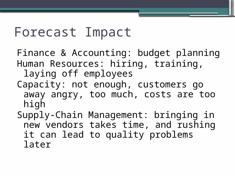
Forecast Impact

Finance & Accounting: budget planningHuman Resources: hiring, training, laying

off employeesCapacity: not enough, customers go away

angry, too much, costs are too highSupply-Chain Management: bringing in

new vendors takes time, and rushing it can lead to quality problems later

Qualitative Methods

•Sales force composite / Grass Roots•Market Research / Consumer market

surveys & interviews•Jury of Executive Opinion / Panel

Consensus•Delphi Method•Historical Analogy - DVDs like VCRs•Naïve approach

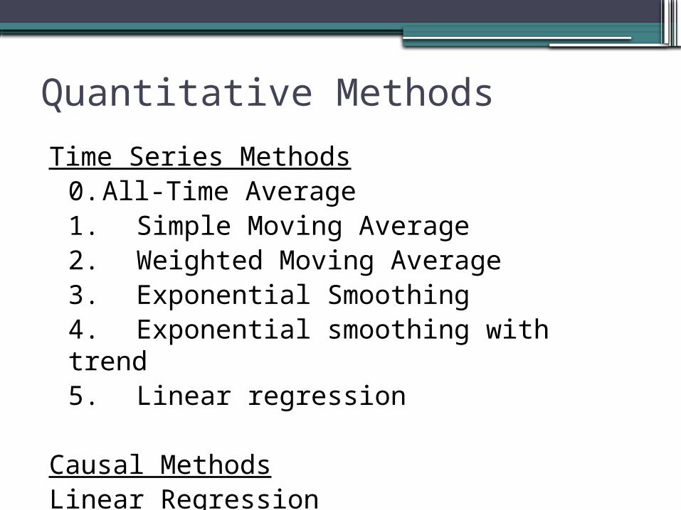
Quantitative Methods

Time Series Methods0. All-Time Average 1. Simple Moving Average2. Weighted Moving Average3. Exponential Smoothing4. Exponential smoothing with trend5. Linear regression

Causal MethodsLinear Regression

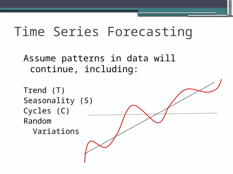
Time Series Forecasting

Assume patterns in data will continue, including:

Trend (T)Seasonality (S)Cycles (C)Random Variations

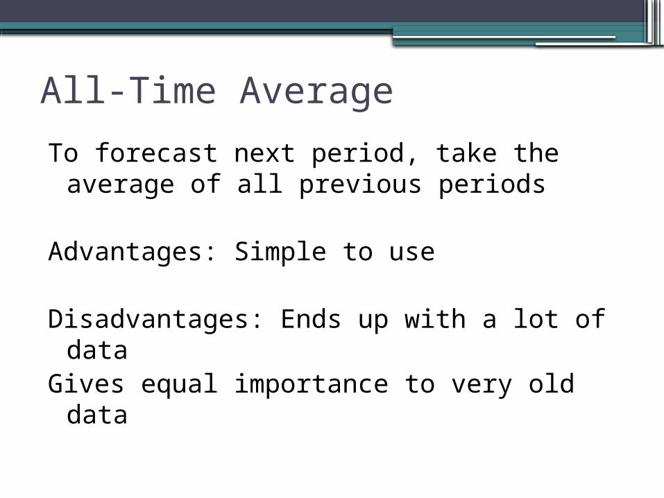
All-Time Average

To forecast next period, take the average of all previous periods

Advantages: Simple to use

Disadvantages: Ends up with a lot of dataGives equal importance to very old data

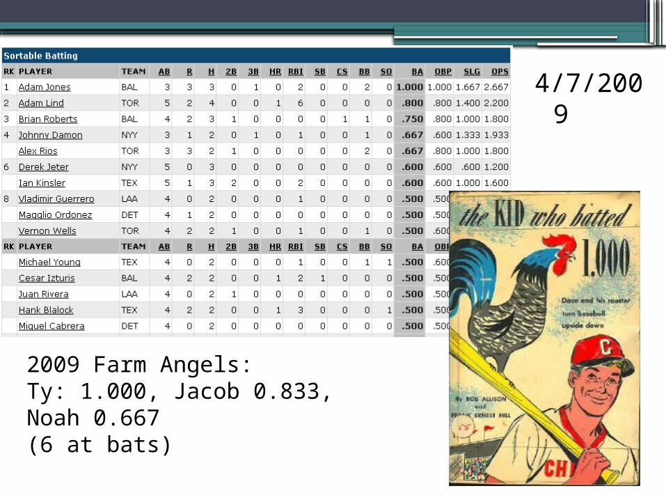
4/7/2009

2009 Farm Angels:Ty: 1.000, Jacob 0.833, Noah 0.667(6 at bats)

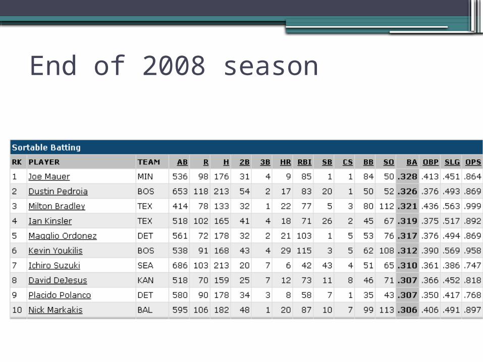
End of 2008 season

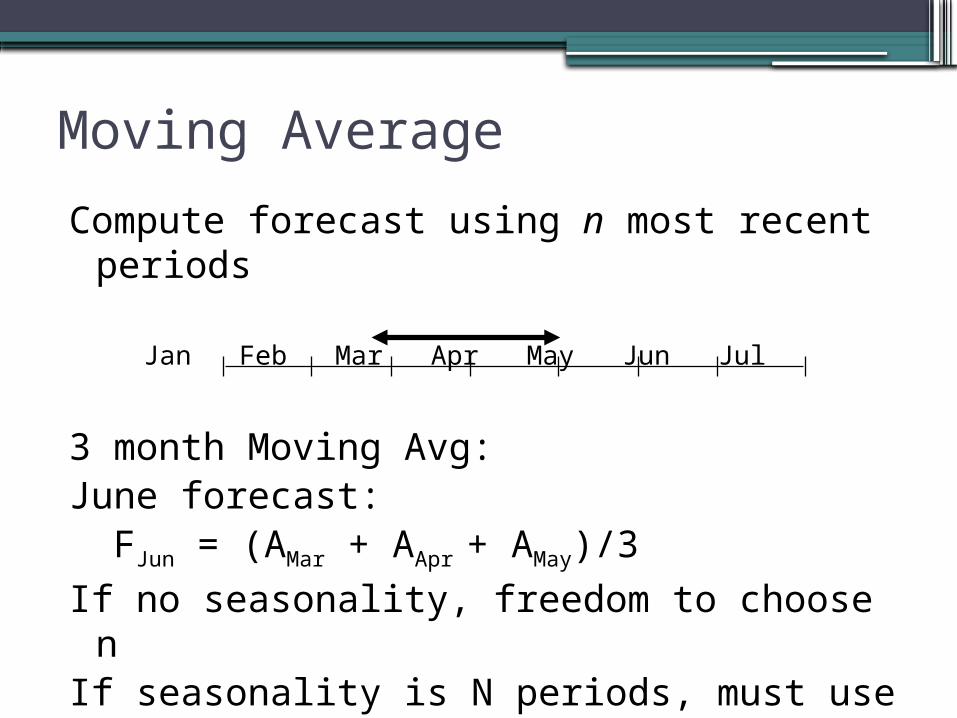
Moving Average

Compute forecast using n most recent periods

Jan Feb Mar Apr May Jun Jul

3 month Moving Avg:June forecast: FJun = (AMar + AApr + AMay)/3

If no seasonality, freedom to choose nIf seasonality is N periods, must use N, 2N,

3N etc. number of periods

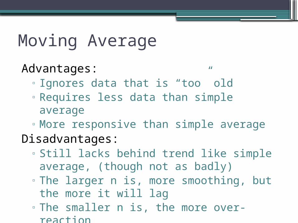
Moving Average

Advantages:▫ Ignores data that is “too” old▫ Requires less data than simple average▫ More responsive than simple average

Disadvantages:▫ Still lacks behind trend like simple average,

(though not as badly)▫ The larger n is, more smoothing, but the

more it will lag▫ The smaller n is, the more over-reaction

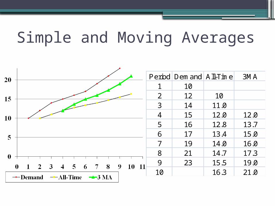
Simple and Moving Averages

Period Demand All-Time 3MA

1 102 12 103 14 11.04 15 12.0 12.05 16 12.8 13.76 17 13.4 15.07 19 14.0 16.08 21 14.7 17.39 23 15.5 19.0

10 16.3 21.0

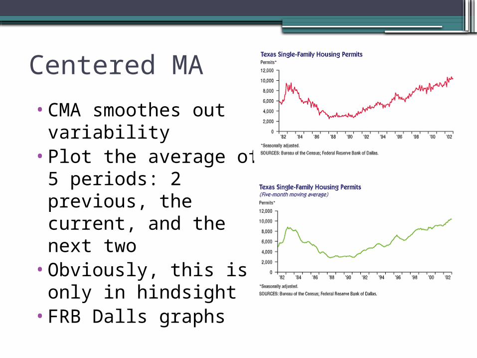
Centered MA

•CMA smoothes out variability

•Plot the average of 5 periods: 2 previous, the current, and the next two

•Obviously, this is only in hindsight

•FRB Dalls graphs

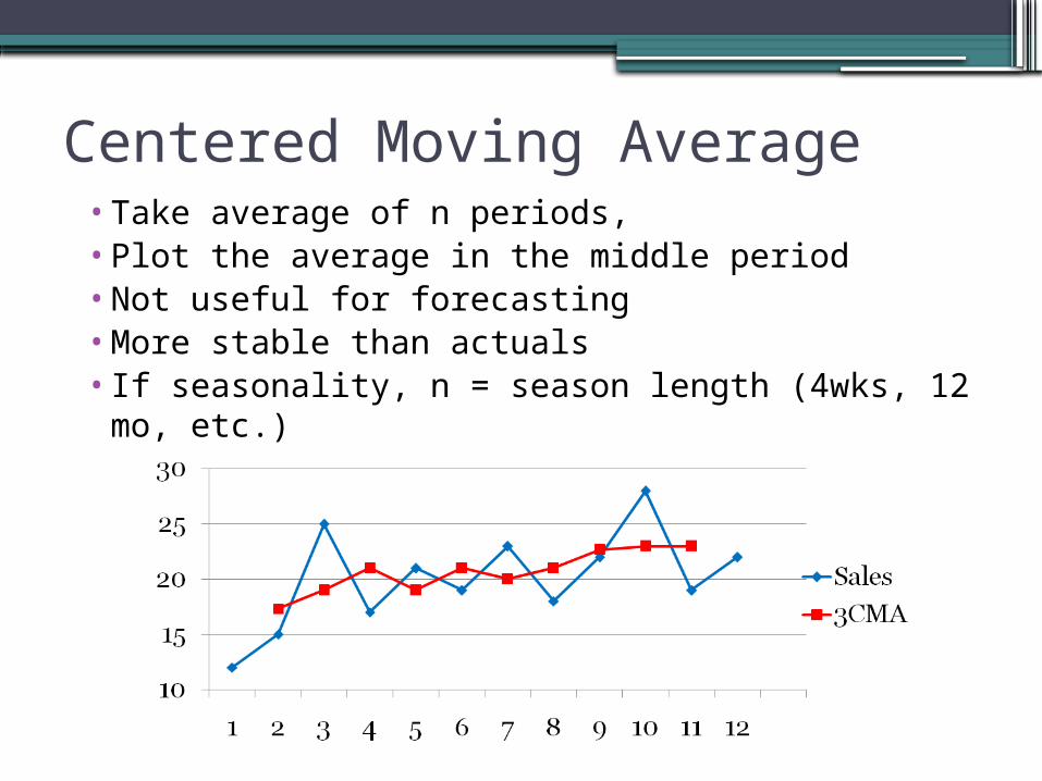
Centered Moving Average• Take average of n periods,• Plot the average in the middle period• Not useful for forecasting• More stable than actuals• If seasonality, n = season length (4wks, 12 mo,

etc.)

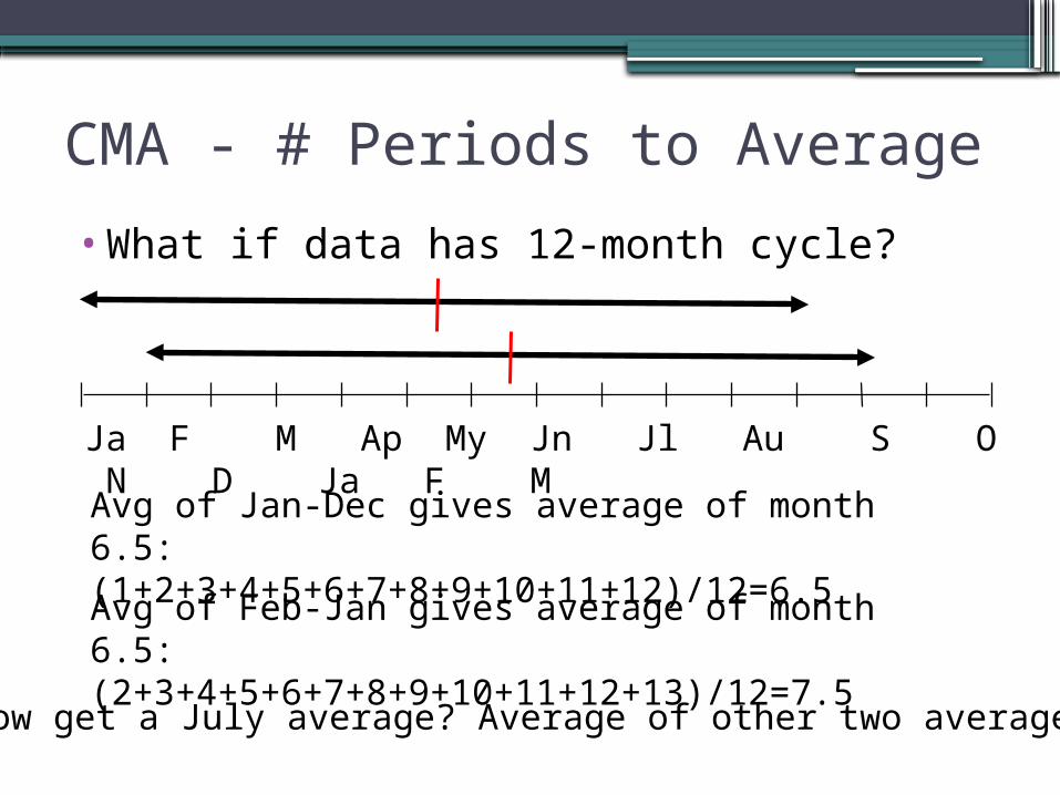
CMA - # Periods to Average

•What if data has 12-month cycle?

Ja F M Ap My Jn Jl Au S O N D Ja F M Avg of Jan-Dec gives average of month 6.5: (1+2+3+4+5+6+7+8+9+10+11+12)/12=6.5Avg of Feb-Jan gives average of month 6.5: (2+3+4+5+6+7+8+9+10+11+12+13)/12=7.5

How get a July average? Average of other two averages

Stability vs. Responsiveness

•Responsive▫Real-time accuracy▫Market conditions

•Stable▫Forecasts being used throughout the

company▫Long-term decisions based on forecasts▫Don’t whipsaw those folks

Centered Moving Average

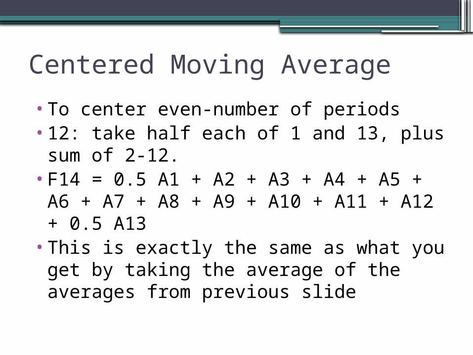
• To center even-number of periods• 12: take half each of 1 and 13, plus sum of

2-12.• F14 = 0.5 A1 + A2 + A3 + A4 + A5 + A6

+ A7 + A8 + A9 + A10 + A11 + A12 + 0.5 A13

• This is exactly the same as what you get by taking the average of the averages from previous slide

Old Data

Comparison of simple, moving averages clearly shows that getting rid of old data makes forecast respond to trends faster

Moving average still lags the trend, but it suggests to us we give newer data more weight, older data less weight.

Weighted Moving Average

FJun = (AMar + AApr + AMay)/3 = (3AMar + 3AApr + 3AMay)/9

Why not consider:FJun = (2AMar + 3AApr + 4AMay)/9FJun = 2/9 AMar + 3/9 AApr + 4/9 AMay

Ft = w1At-3 + w2At-2 + w3At-1

Complicated:• Have to decide number of periods, and weights for each• Weights have to add up to 1.0• Most recent probably most relevant, gets most weight• Carry around n periods of data to make new forecast

Weighted Moving Average

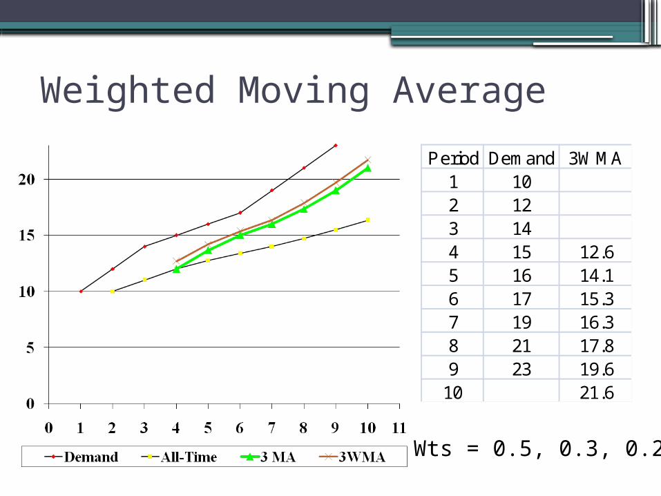
Period Demand 3WMA1 102 123 144 15 12.65 16 14.16 17 15.37 19 16.38 21 17.89 23 19.6

10 21.6

Wts = 0.5, 0.3, 0.2

Setting Parameters

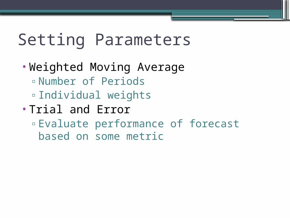
•Weighted Moving Average▫Number of Periods▫Individual weights

•Trial and Error▫Evaluate performance of forecast based on

some metric

Exponential Smoothing

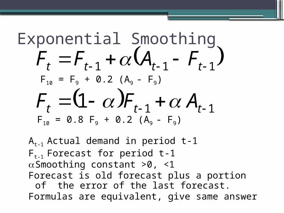
At-1 Actual demand in period t-1 Ft-1 Forecast for period t-1 Smoothing constant >0, <1Forecast is old forecast plus a portion of the

error of the last forecast.Formulas are equivalent, give same answer

111 tttt FAFF F10 = F9 + 0.2 (A9 - F9)

111 ttt AFF F10 = 0.8 F9 + 0.2 (A9 - F9)

Exponential Smoothing

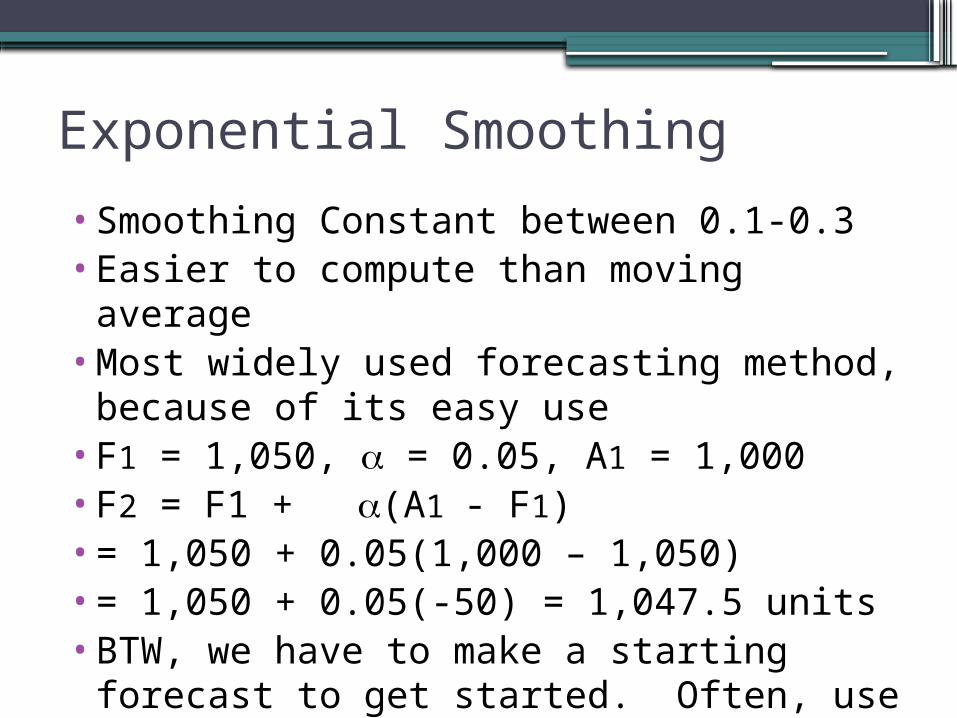
•Smoothing Constant between 0.1-0.3•Easier to compute than moving average•Most widely used forecasting method,

because of its easy use•F1 = 1,050, = 0.05, A1 = 1,000•F2 = F1 + (A1 - F1) •= 1,050 + 0.05(1,000 – 1,050)•= 1,050 + 0.05(-50) = 1,047.5 units•BTW, we have to make a starting forecast

to get started. Often, use actual A1

Exponential Smoothing

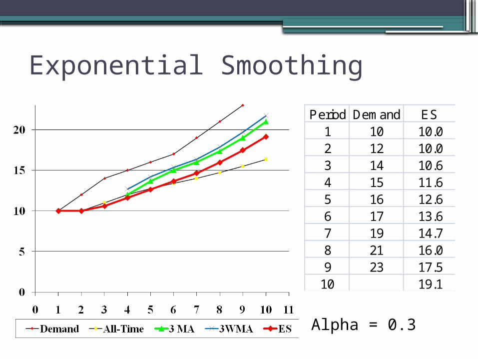
Period Demand ES1 10 10.02 12 10.03 14 10.64 15 11.65 16 12.66 17 13.67 19 14.78 21 16.09 23 17.5

10 19.1

Alpha = 0.3

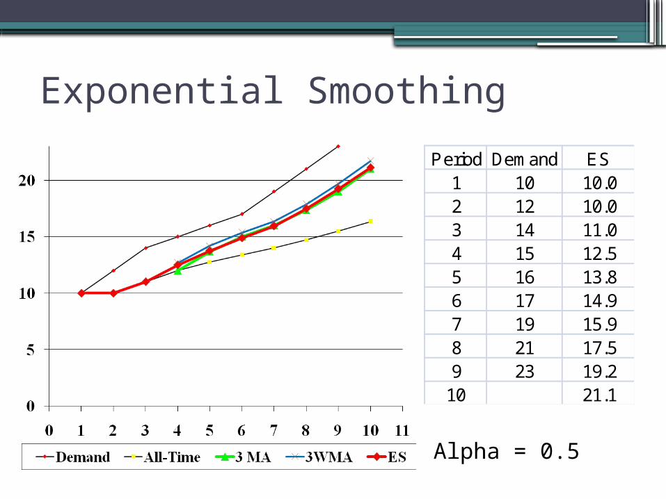
Exponential Smoothing

Period Demand ES1 10 10.02 12 10.03 14 11.04 15 12.55 16 13.86 17 14.97 19 15.98 21 17.59 23 19.2

10 21.1

Alpha = 0.5

Exponential Smoothing

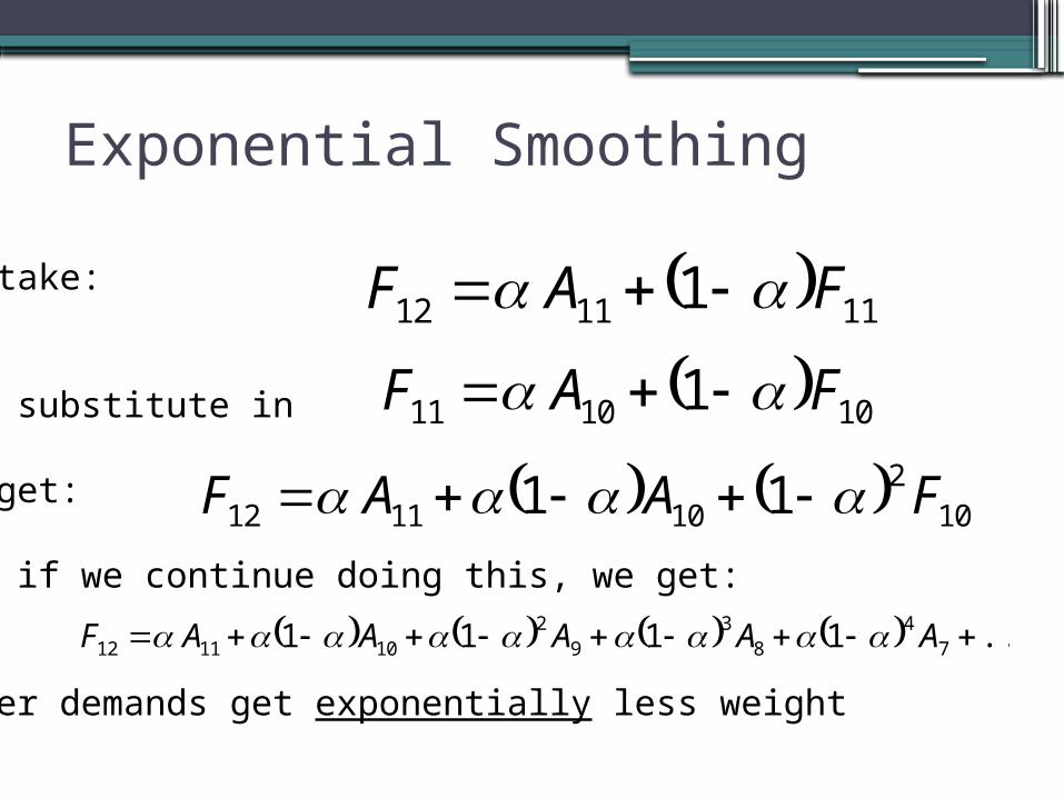
111112 1 FAF

101011 1 FAF

We take:

And substitute in

to get:

and if we continue doing this, we get:

Older demands get exponentially less weight

102

101112 11 FAAF

...1111 74

83

92

101112 AAAAAF

Choosing

•Low : if demand is stable, we don’t want to get thrown into a wild-goose chase, over-reacting to “trends” that are really just short-term variation

•High : If demand really is changing rapidly, we want to react as quickly as possible

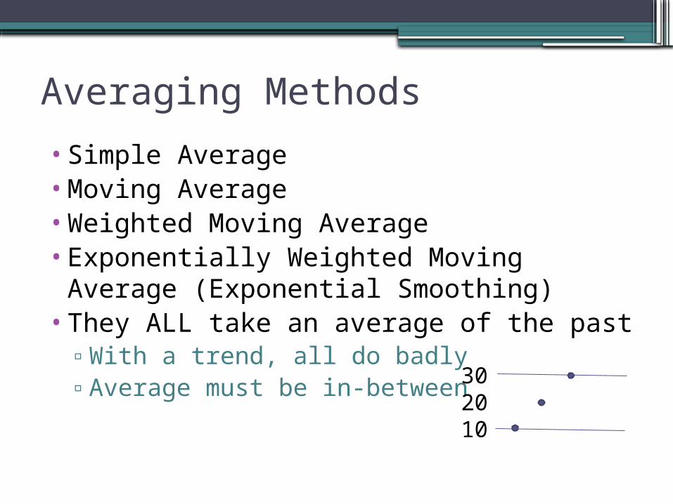
Averaging Methods

•Simple Average•Moving Average•Weighted Moving Average•Exponentially Weighted Moving Average

(Exponential Smoothing)•They ALL take an average of the past

▫With a trend, all do badly▫Average must be in-between 30

2010

Trend-Adjusted Ex. Smoothing

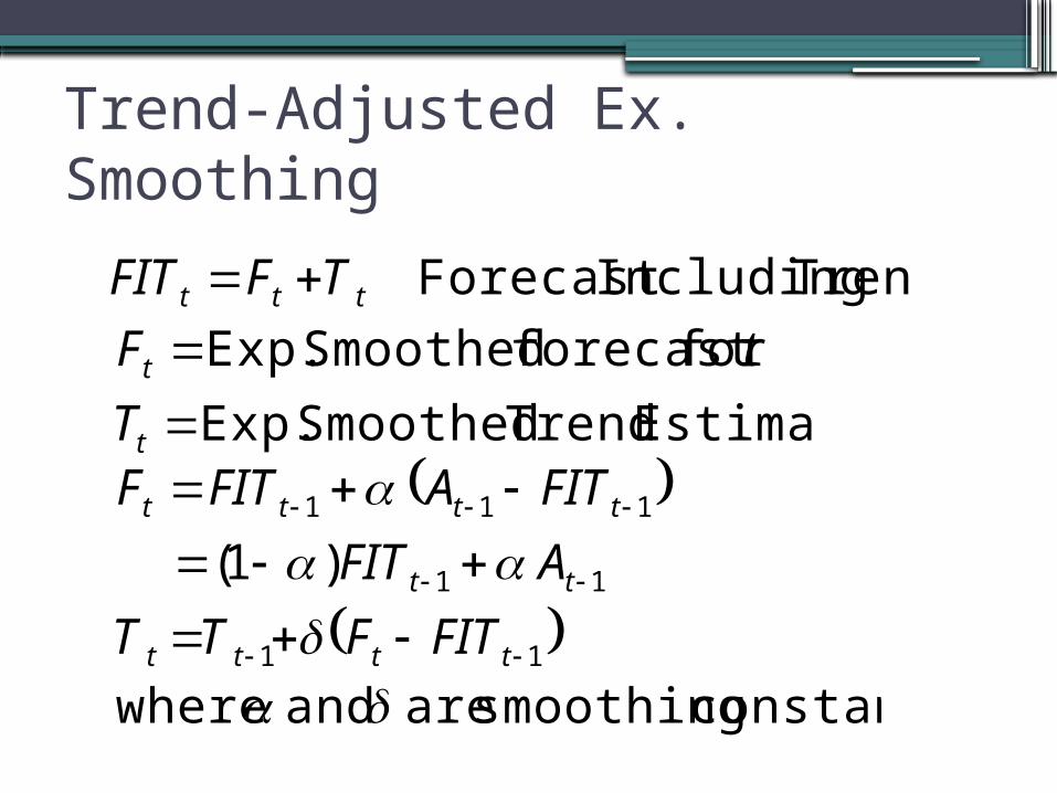
Trend IncludingForecast ttt TFFIT

Estimate Trend Smoothed Exp.

for forecast Smoothed Exp.

t

t

T

tF

11

11

111

)1(

tttt

tt

tttt

FITFTT

AFIT

FITAFITF

constants smoothing are and where

Trend-Adjusted Ex. Smoothing

3.103.010)110111(*30.010

121112

FITFTFITFTT ttt

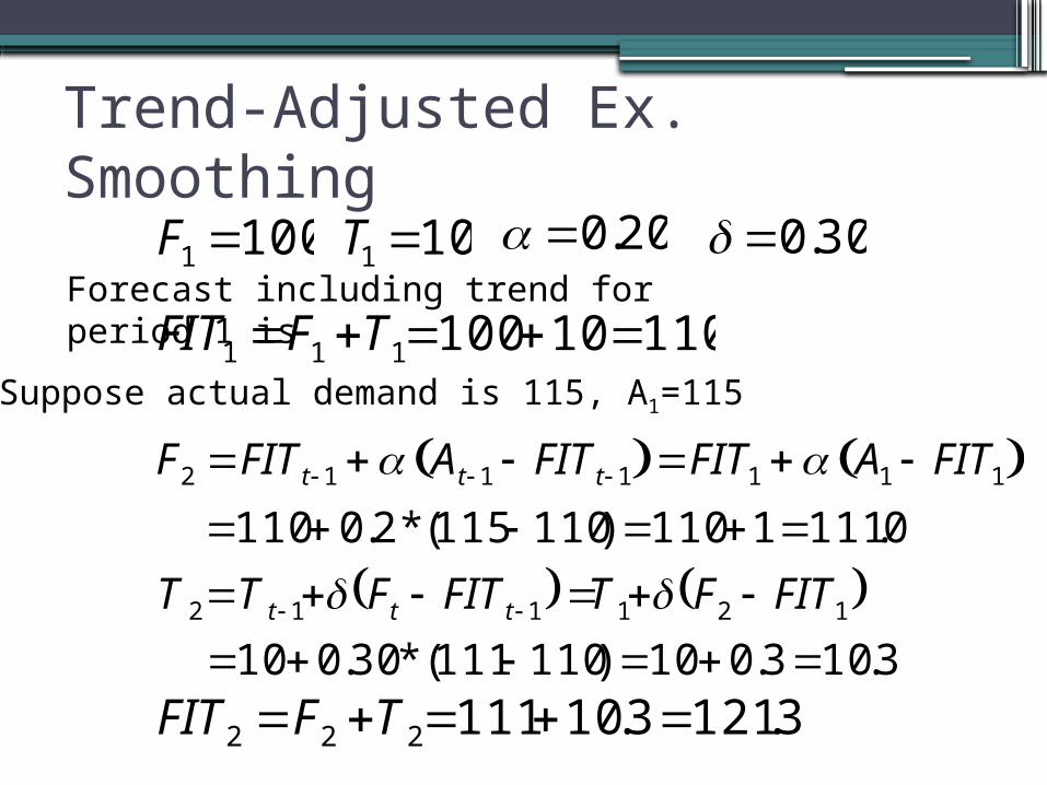
F1 100

T1 10

0.20

0.30Forecast including trend for period 1 is

FIT1 F1 T1100 10 110

F2 FITt 1 At 1 FITt 1 FIT1 A1 FIT1 110 0.2*(115 110) 110 1111.0

Suppose actual demand is 115, A1=115

FIT2 F2 T 2111 10.3 121.3

Trend-Adjusted Ex. Smoothing

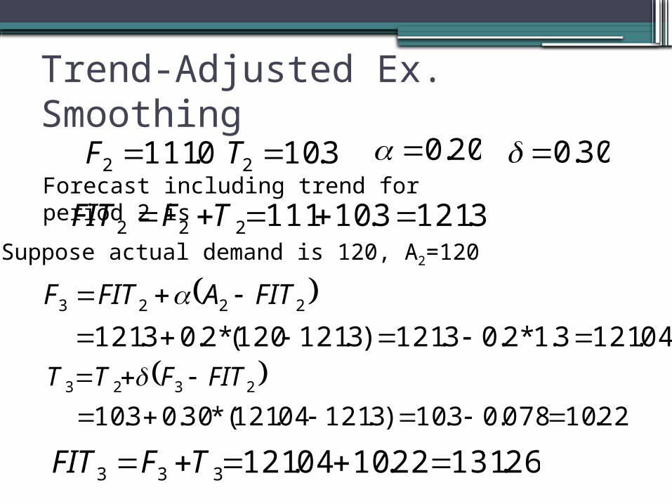
22.10078.03.10)3.12104.121(*30.03.10

2323

FITFTT

0.1112 F 3.102 T

0.20

0.30Forecast including trend for period 2 is

3.1213.10111222 TFFIT

04.1213.1*2.03.121)3.121120(*2.03.121

2223

FITAFITF

Suppose actual demand is 120, A2=120

26.13122.1004.121333 TFFIT

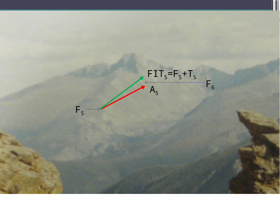
F5

FIT5=F5+T5

A5

F6

Selecting and

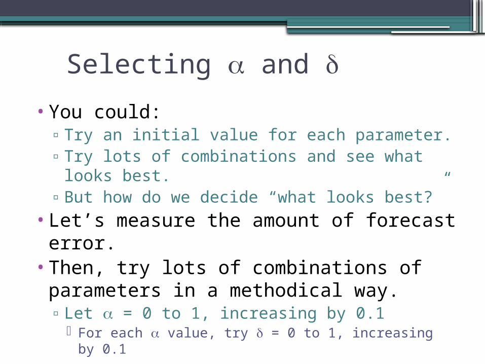
•You could:▫Try an initial value for each parameter.▫Try lots of combinations and see what looks

best.▫But how do we decide “what looks best?”

•Let’s measure the amount of forecast error.

•Then, try lots of combinations of parameters in a methodical way.▫Let = 0 to 1, increasing by 0.1

For each value, try = 0 to 1, increasing by 0.1

Evaluating Forecasts

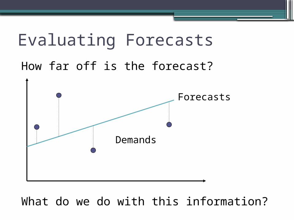
How far off is the forecast?

What do we do with this information?

Forecasts

Demands

Measuring the ErrorsPeriod A-F

Method 1

A-FMethod 2

1 100 10

2 -100 10

3 100 10

4 -100 10

5 100 10

6 -100 10

7 100 10

8 -100 10

9 100 10

10 -100 10

RSFE 0 100

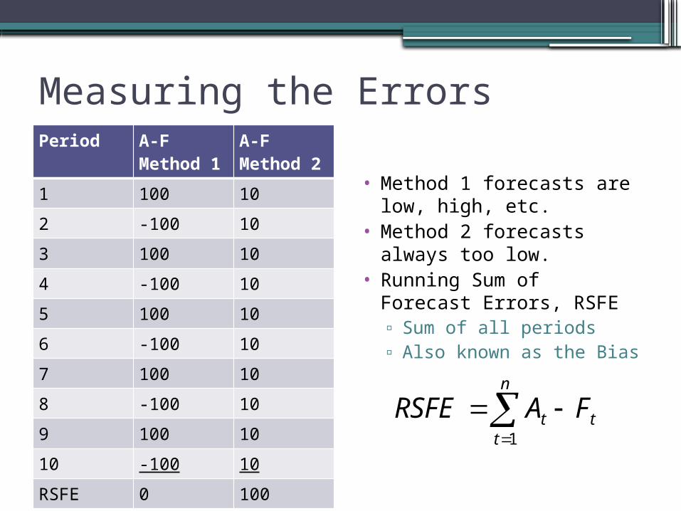
• Method 1 forecasts are low, high, etc.

• Method 2 forecasts always too low.

• Running Sum of Forecast Errors, RSFE▫ Sum of all periods▫ Also known as the Bias

n

ttt FARSFE

1

Evaluating Forecasts

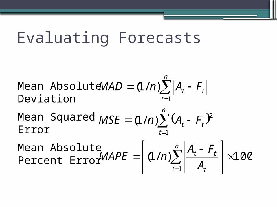
Mean Absolute Deviation

Mean Squared Error

Mean Absolute Percent Error

100)/1(

)/1(

)/1(

1

1

2

1

n

t t

tt

n

ttt

n

ttt

A

FAnMAPE

FAnMSE

FAnMAD

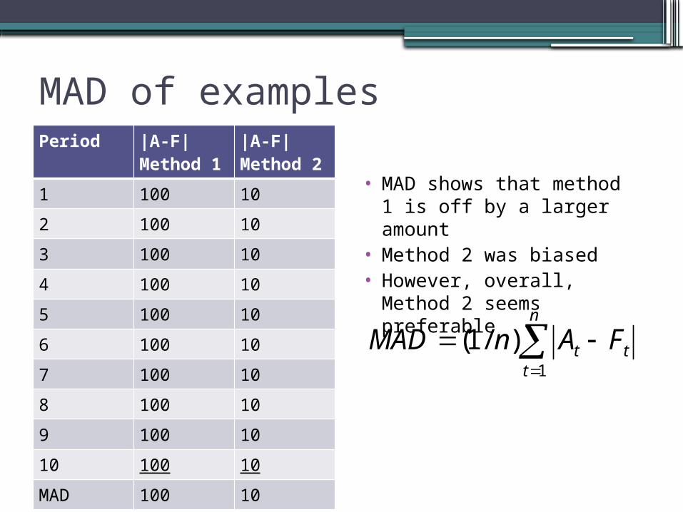
MAD of examplesPeriod |A-F|

Method 1

|A-F|Method 2

1 100 10

2 100 10

3 100 10

4 100 10

5 100 10

6 100 10

7 100 10

8 100 10

9 100 10

10 100 10

MAD 100 10

• MAD shows that method 1 is off by a larger amount

• Method 2 was biased• However, overall, Method

2 seems preferable

n

ttt FAnMAD

1

)/1(

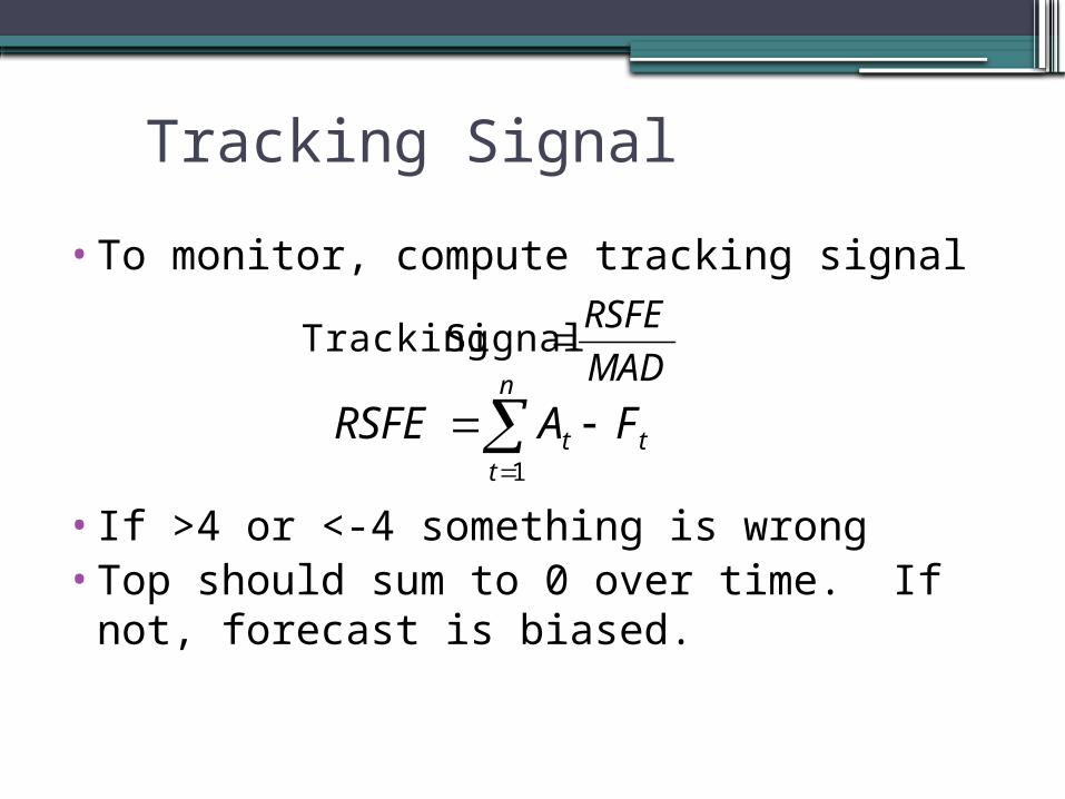
Tracking Signal

•To monitor, compute tracking signal

•If >4 or <-4 something is wrong•Top should sum to 0 over time. If not,

forecast is biased.

n

ttt FARSFE

1

MAD

RSFESignal Tracking

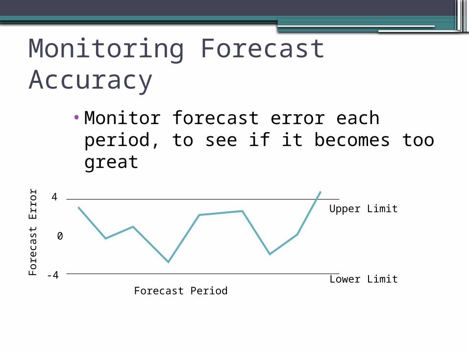
Monitoring Forecast Accuracy

•Monitor forecast error each period, to see if it becomes too great

0

-4

4

Fore

cast

Err

or

Forecast PeriodLower Limit

Upper Limit

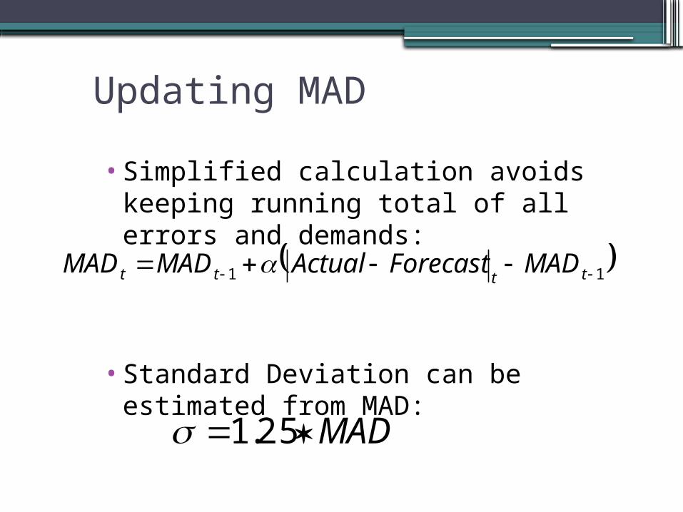
Updating MAD

•Simplified calculation avoids keeping running total of all errors and demands:

•Standard Deviation can be estimated from MAD:

MAD 25.1

11 tttt MADForecastActualMADMAD

Techniques for Trend

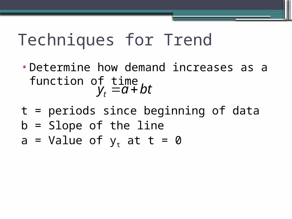
•Determine how demand increases as a function of time

t = periods since beginning of datab = Slope of the linea = Value of yt at t = 0

btayt

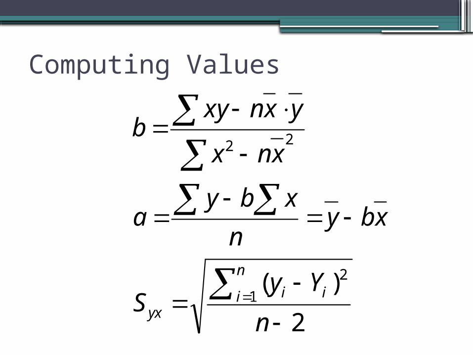
Computing Values

2

)(1

2

22

n

YyS

xbyn

xbya

xnx

yxnxyb

n

i iiyx

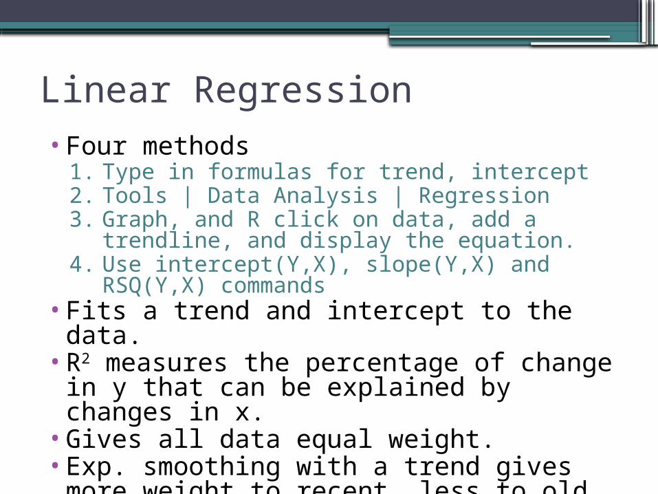
Linear Regression•Four methods

1. Type in formulas for trend, intercept2. Tools | Data Analysis | Regression3. Graph, and R click on data, add a trendline,

and display the equation.4. Use intercept(Y,X), slope(Y,X) and RSQ(Y,X)

commands•Fits a trend and intercept to the data.•R2 measures the percentage of change in

y that can be explained by changes in x.•Gives all data equal weight.•Exp. smoothing with a trend gives more

weight to recent, less to old.

Causal Forecasting

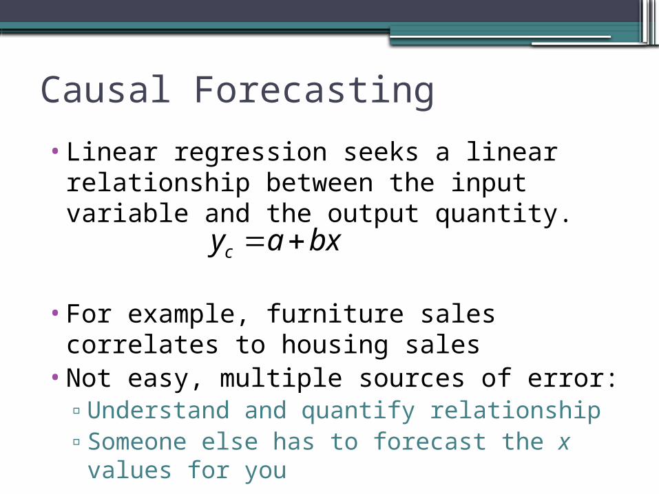
•Linear regression seeks a linear relationship between the input variable and the output quantity.

•For example, furniture sales correlates to housing sales

•Not easy, multiple sources of error:▫Understand and quantify relationship▫Someone else has to forecast the x values

for you

bxayc

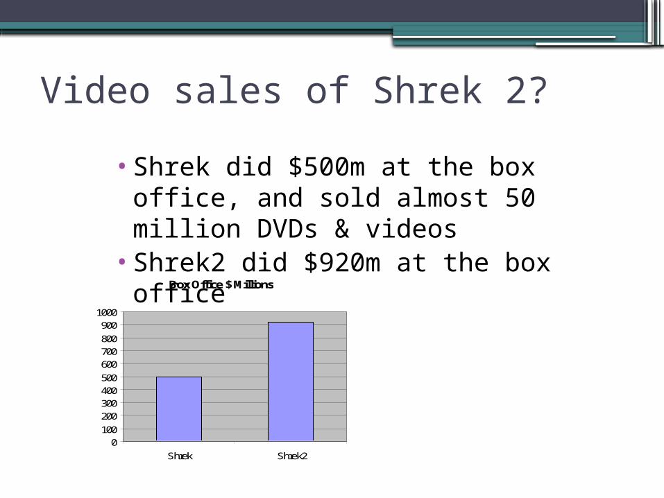
Video sales of Shrek 2?

Box Office $ Millions

0100

200300400500

600700800

9001000

Shrek Shrek2

•Shrek did $500m at the box office, and sold almost 50 million DVDs & videos

•Shrek2 did $920m at the box office

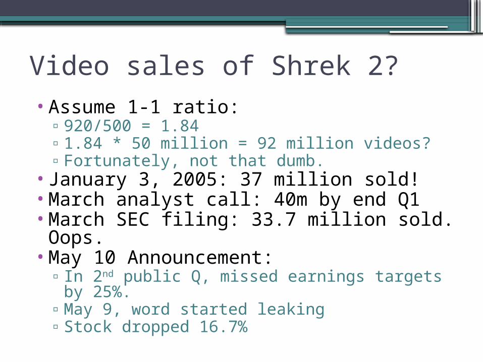
Video sales of Shrek 2?•Assume 1-1 ratio:

▫920/500 = 1.84▫1.84 * 50 million = 92 million videos?▫Fortunately, not that dumb.

•January 3, 2005: 37 million sold!•March analyst call: 40m by end Q1•March SEC filing: 33.7 million sold. Oops.•May 10 Announcement:

▫In 2nd public Q, missed earnings targets by 25%.

▫May 9, word started leaking▫Stock dropped 16.7%

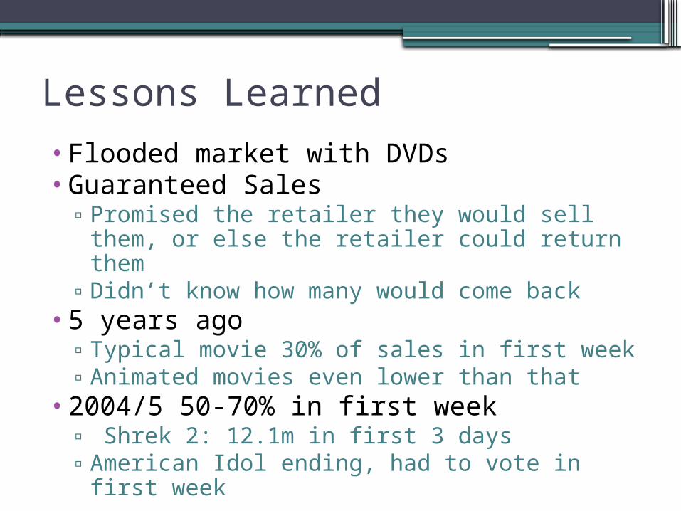
Lessons Learned

•Flooded market with DVDs•Guaranteed Sales

▫Promised the retailer they would sell them, or else the retailer could return them

▫Didn’t know how many would come back•5 years ago

▫Typical movie 30% of sales in first week▫Animated movies even lower than that

•2004/5 50-70% in first week▫ Shrek 2: 12.1m in first 3 days▫American Idol ending, had to vote in first week

The Human Element

•Colbert says you have more nerve endings in your gut than in your brain

•Limited ability to include factors▫Can’t include everything

•If it feels really wrong to your gut, maybe your gut is right

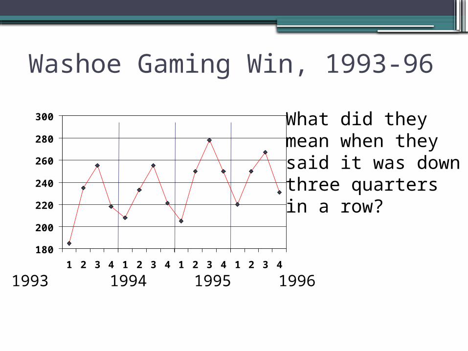
Washoe Gaming Win, 1993-96

180

200

220

240

260

280

300

1 2 3 4 1 2 3 4 1 2 3 4 1 2 3 4

What did they mean when they said it was down three quartersin a row?

1993 1994 1995 1996

Seasonality

•Seasonality is regular up or down movements in the data

•Can be hourly, daily, weekly, yearly•Naïve method

▫N1: Assume January sales will be same as December

▫N2: Assume this Friday’s ticket sales will be same as last

Seasonal Factors

•Seasonal factor for May is 1.20, means May sales are typically 20% above the average

•Factor for July is 0.90, meaning July sales are typically 10% below the average

Seasonality & No Trend

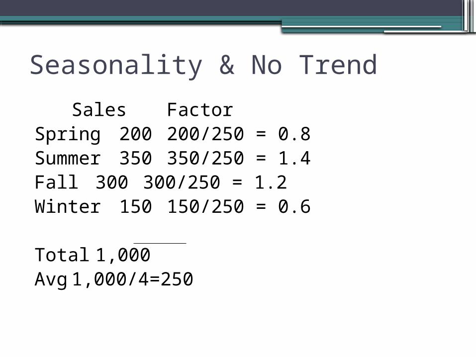
Sales FactorSpring 200 200/250 = 0.8Summer 350 350/250 = 1.4Fall 300 300/250 = 1.2Winter 150 150/250 = 0.6

Total 1,000Avg 1,000/4=250

Seasonality & No Trend

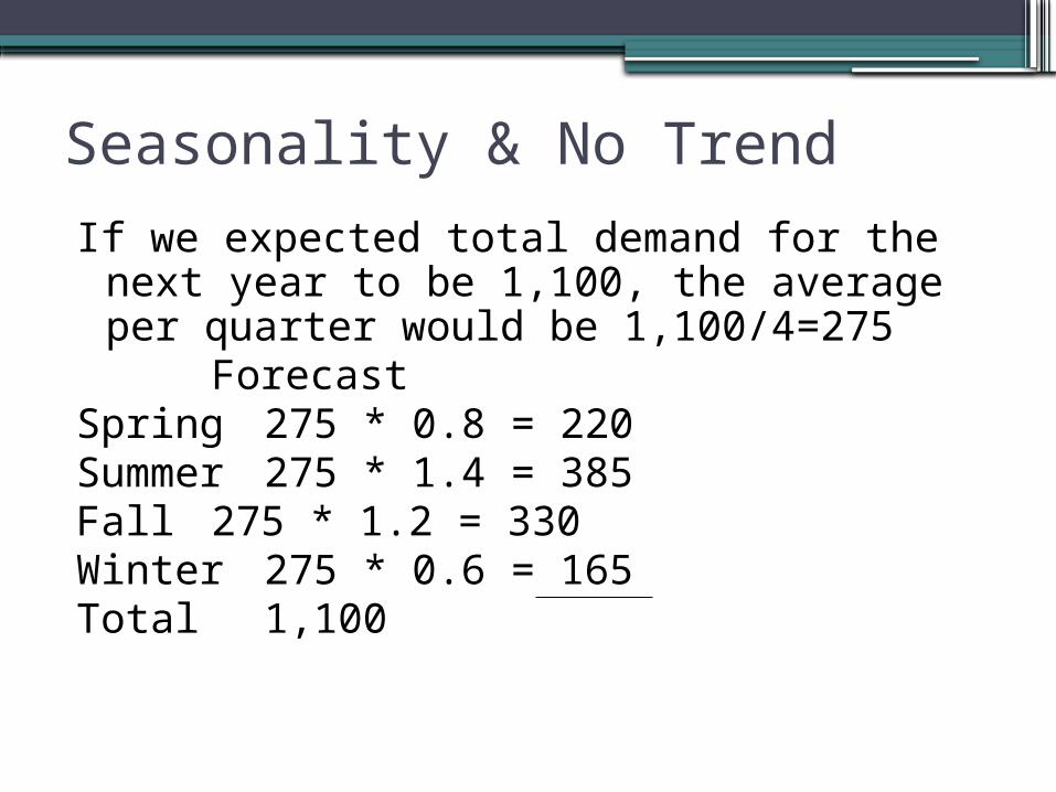
If we expected total demand for the next year to be 1,100, the average per quarter would be 1,100/4=275

ForecastSpring 275 * 0.8 = 220Summer 275 * 1.4 = 385Fall 275 * 1.2 = 330Winter 275 * 0.6 = 165Total 1,100

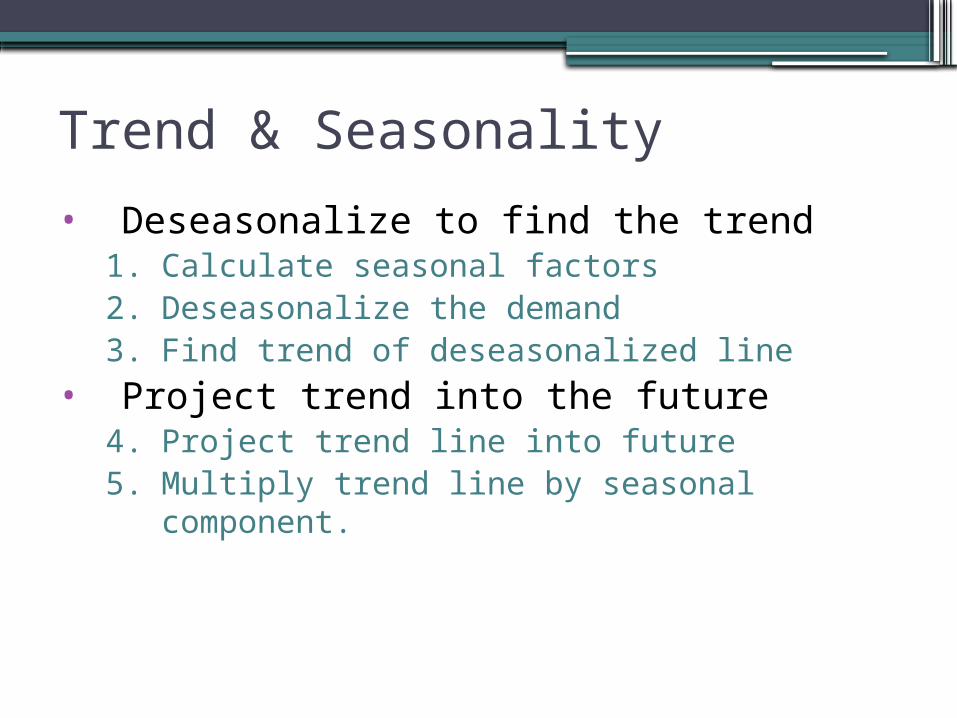
Trend & Seasonality

• Deseasonalize to find the trend1. Calculate seasonal factors2. Deseasonalize the demand3. Find trend of deseasonalized line

• Project trend into the future4. Project trend line into future5. Multiply trend line by seasonal component.

Washoe Gaming Win, 1993-96

180

200

220

240

260

280

300

1 2 3 4 1 2 3 4 1 2 3 4 1 2 3 4

Looks like a downhill slide- Silver Legacy

opened 95Q3- Otherwise,

upward trend

1993 1994 1995 1996

Source: Comstock Bank, Survey of Nevada Business & Economics

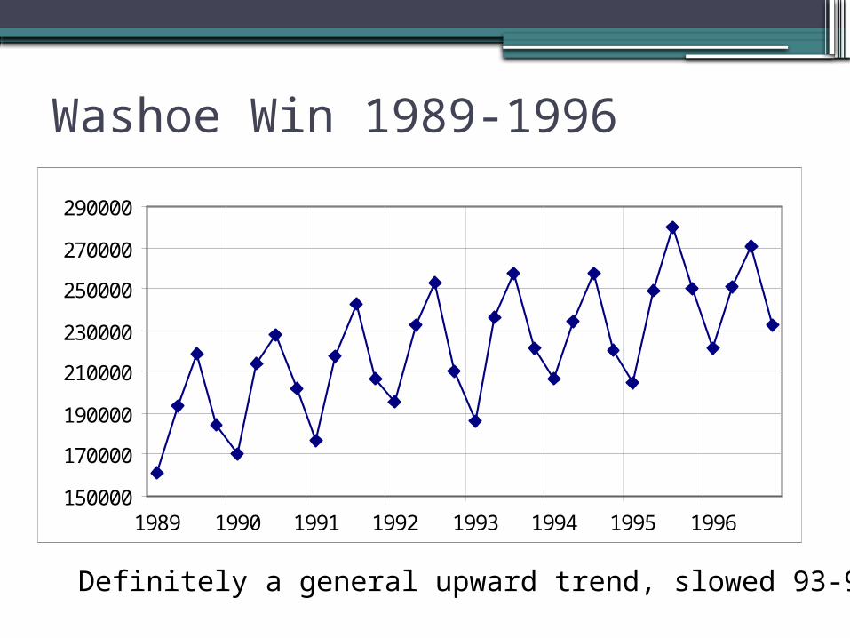
Washoe Win 1989-1996

150000

170000

190000

210000

230000

250000

270000

290000

1989 1990 1991 1992 1993 1994 1995 1996

Definitely a general upward trend, slowed 93-94

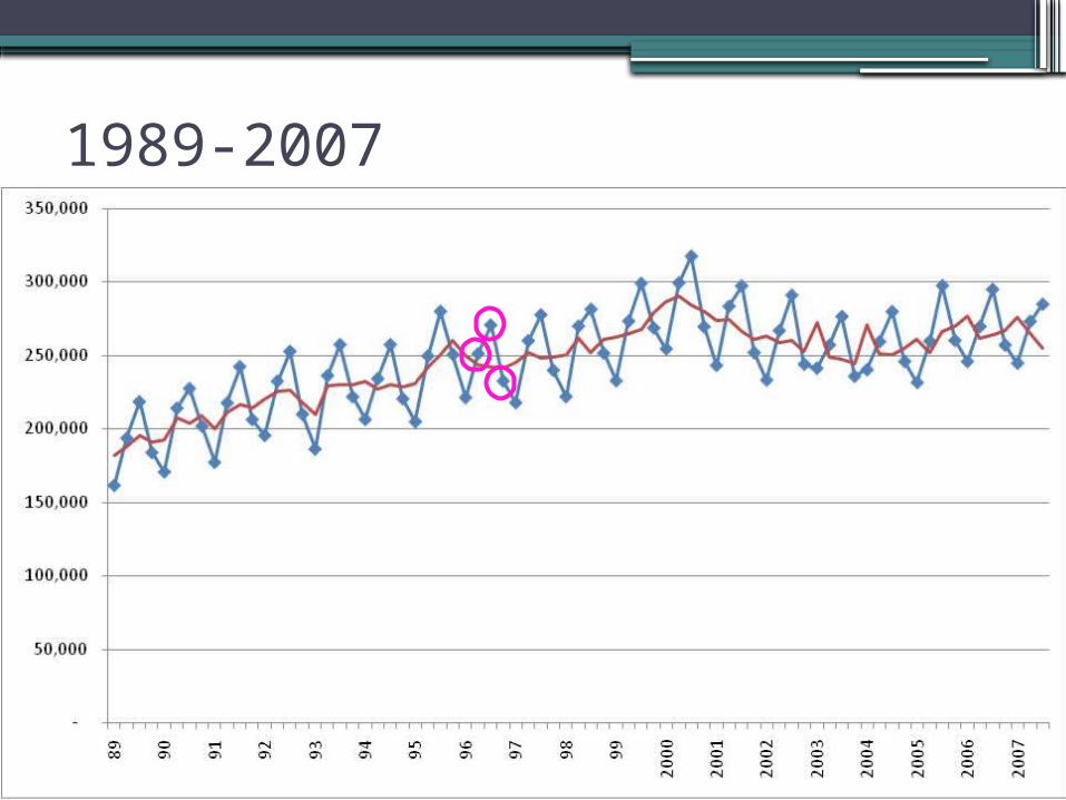
1989-2007

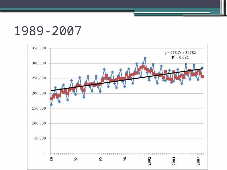
1989-2007

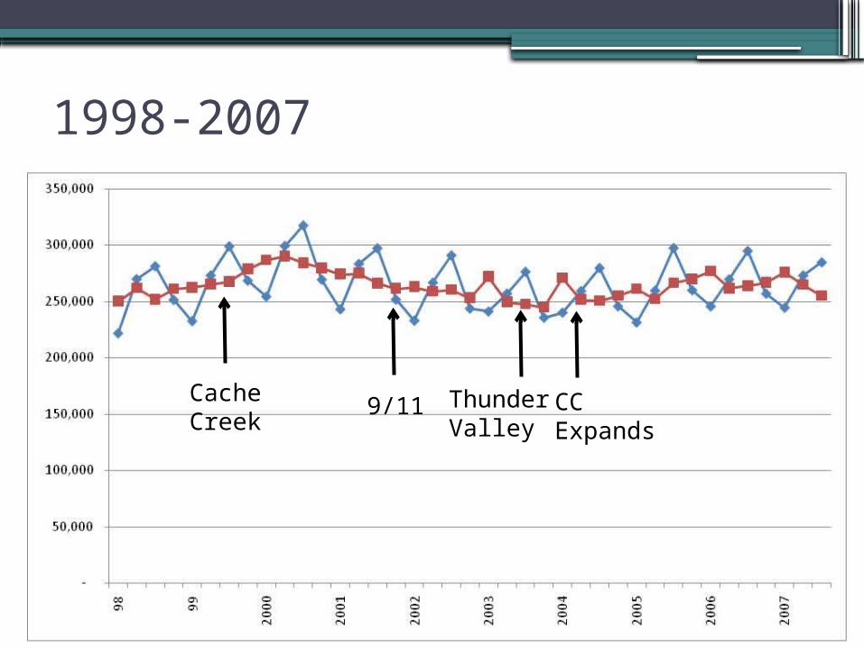
1998-2007

CacheCreek

ThunderValley

CCExpands

9/11

Centered Moving Average

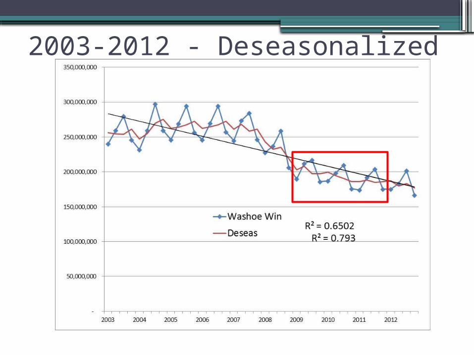
2003-2012 - Deseasonalized

2003 2004 2005 2006 2007 2008 2009 2010 2011 -

50,000,000

100,000,000

150,000,000

200,000,000

250,000,000

300,000,000

350,000,000

Washoe Win

Linear

Forecast

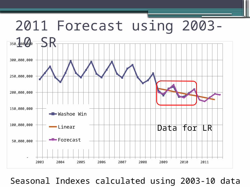
2011 Forecast using 2003-10 SR

Data for LR

Seasonal Indexes calculated using 2003-10 data

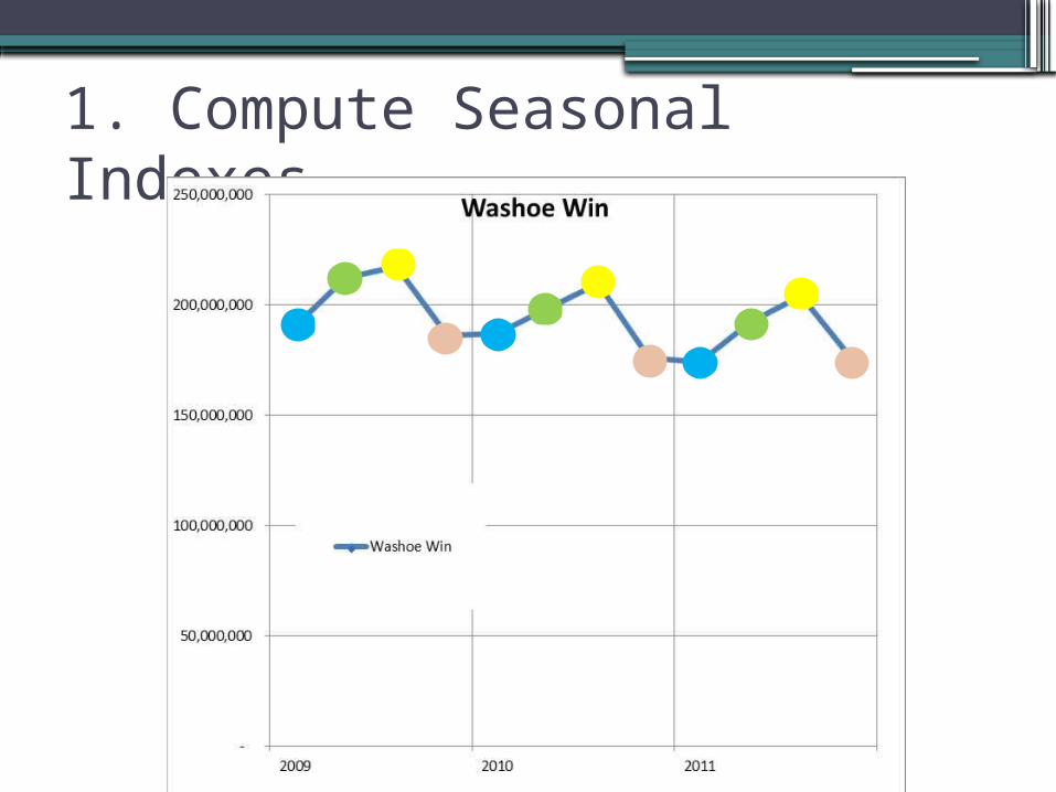
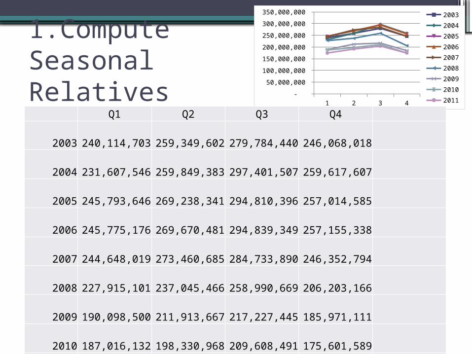
1. Compute Seasonal Indexes

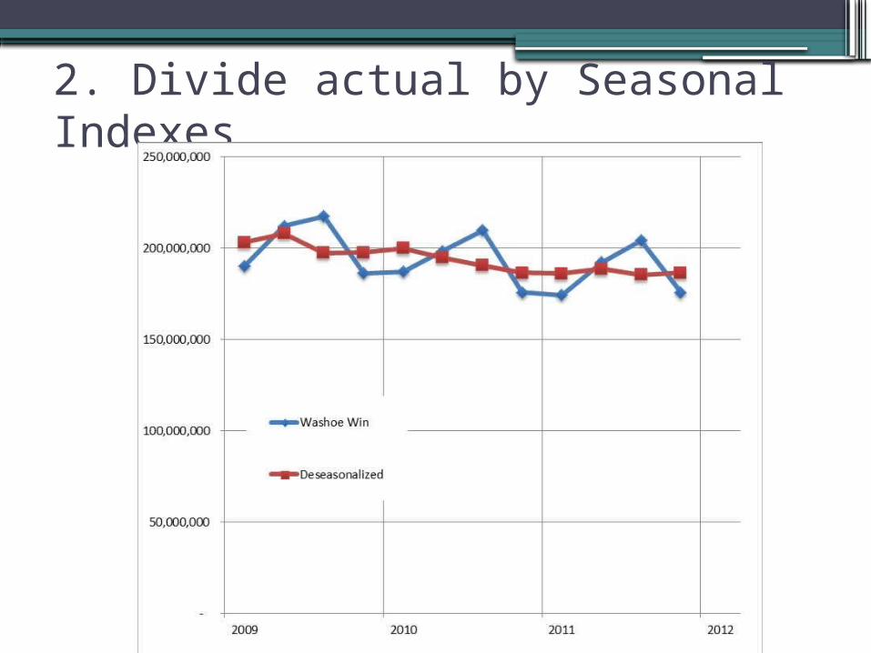
2. Divide actual by Seasonal Indexes

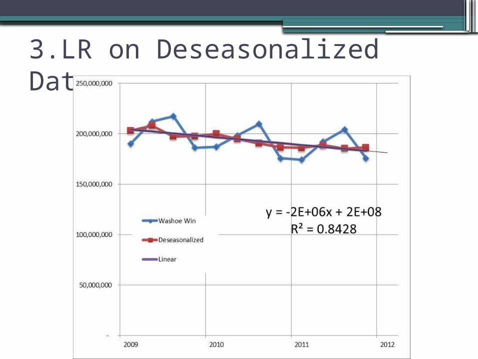
3.LR on Deseasonalized Data

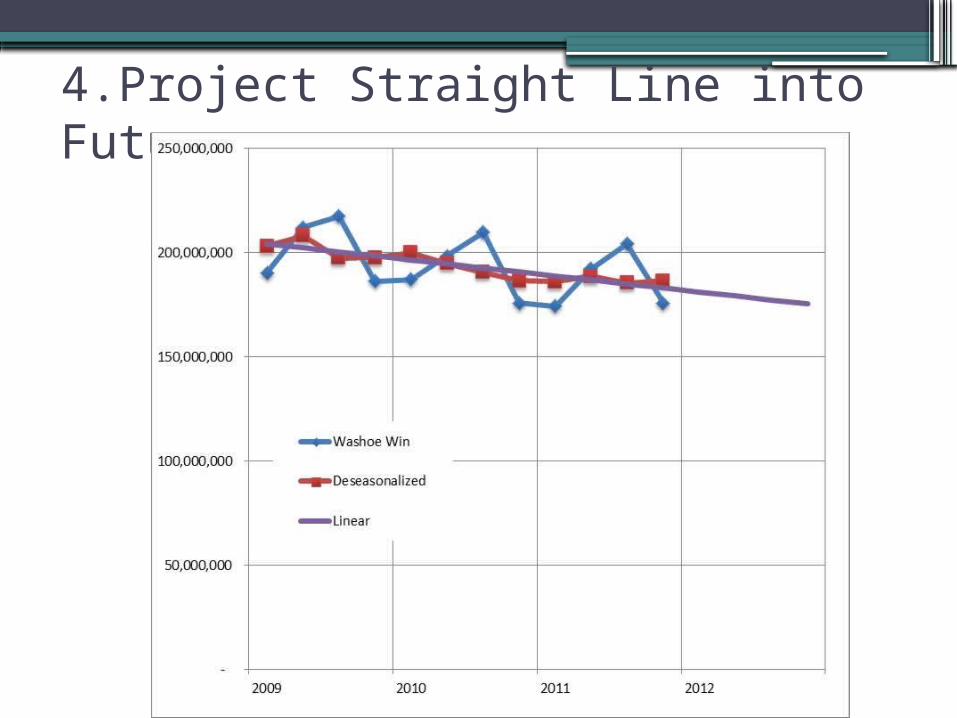
4.Project Straight Line into Future

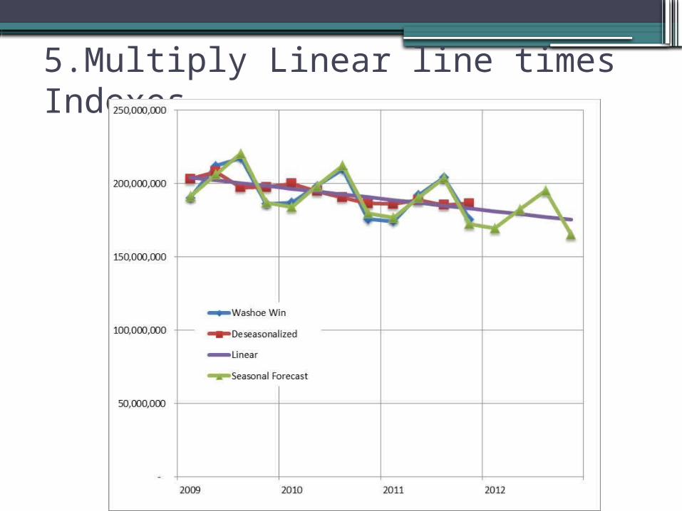
5.Multiply Linear line times Indexes

How Did We Do? – 2012 Actual Win

1 2 3 4 -

50,000,000

100,000,000

150,000,000

200,000,000

250,000,000

300,000,000

350,000,000 200320042005200620072008200920102011

1.Compute Seasonal Relatives

Q1 Q2 Q3 Q4

2003 240,114,703 259,349,602 279,784,440 246,068,018

2004 231,607,546 259,849,383 297,401,507 259,617,607

2005 245,793,646 269,238,341 294,810,396 257,014,585

2006 245,775,176 269,670,481 294,839,349 257,155,338

2007 244,648,019 273,460,685 284,733,890 246,352,794

2008 227,915,101 237,045,466 258,990,669 206,203,166

2009 190,098,500 211,913,667 217,227,445 185,971,111

2010 187,016,132 198,330,968 209,608,491 175,601,589

2011 174,138,905 192,122,889 203,912,214 175,510,911

avg 220,789,748 241,220,165 260,145,378 223,277,235 236,358,131

SR

0.934

1.021

1.101

0.945

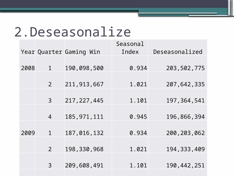
2.DeseasonalizeYear Quarter Gaming Win

Seasonal Index Deseasonalized

2008 1 190,098,500

0.934 203,502,775

2 211,913,667

1.021 207,642,335

3 217,227,445

1.101 197,364,541

4 185,971,111

0.945 196,866,394

2009 1 187,016,132

0.934 200,203,062

2 198,330,968

1.021 194,333,409

3 209,608,491

1.101 190,442,251

4 175,601,589

0.945 185,889,365

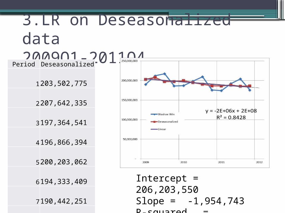
3.LR on Deseasonalized data 2009Q1-2011Q4

Period Deseasonalized1 203,502,775 2 207,642,335 3 197,364,541 4 196,866,394 5 200,203,062 6 194,333,409 7 190,442,251 8 185,889,365 9 186,417,833

10 188,250,460 11 185,266,831 12 185,793,374

Intercept = 206,203,550Slope = -1,954,743R-squared =0.848

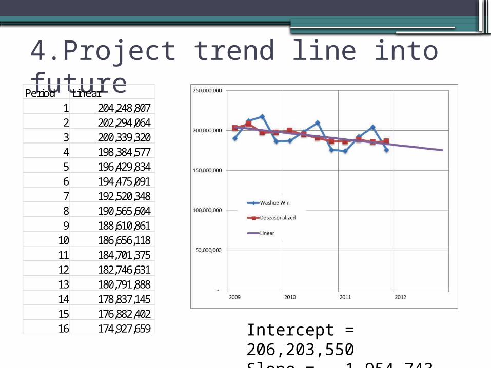
4.Project trend line into future

Intercept = 206,203,550Slope = -1,954,743

Period Linear1 204,248,807 2 202,294,064 3 200,339,320 4 198,384,577 5 196,429,834 6 194,475,091 7 192,520,348 8 190,565,604 9 188,610,861

10 186,656,118 11 184,701,375 12 182,746,631 13 180,791,888 14 178,837,145 15 176,882,402 16 174,927,659

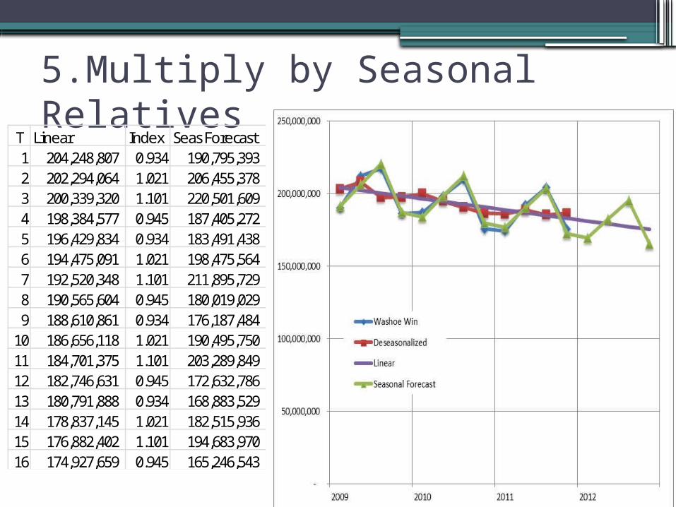
5.Multiply by Seasonal Relatives

T Linear Index Seas Forecast1 204,248,807 0.934 190,795,393 2 202,294,064 1.021 206,455,378 3 200,339,320 1.101 220,501,609 4 198,384,577 0.945 187,405,272 5 196,429,834 0.934 183,491,438 6 194,475,091 1.021 198,475,564 7 192,520,348 1.101 211,895,729 8 190,565,604 0.945 180,019,029 9 188,610,861 0.934 176,187,484

10 186,656,118 1.021 190,495,750 11 184,701,375 1.101 203,289,849 12 182,746,631 0.945 172,632,786 13 180,791,888 0.934 168,883,529 14 178,837,145 1.021 182,515,936 15 176,882,402 1.101 194,683,970 16 174,927,659 0.945 165,246,543

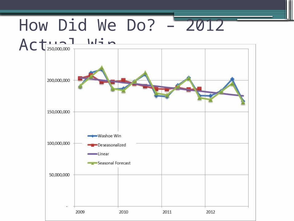
How Did We Do? – 2012 Actual Win

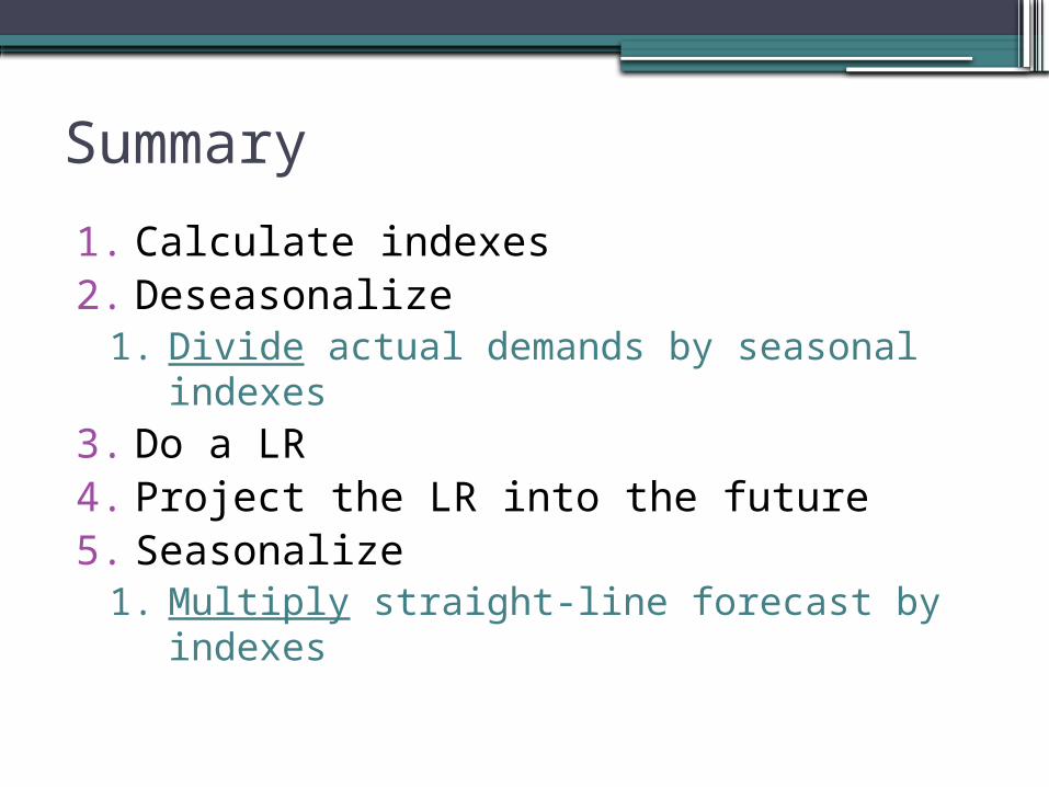
Summary

1. Calculate indexes2. Deseasonalize

1. Divide actual demands by seasonal indexes

3. Do a LR4. Project the LR into the future5. Seasonalize

1. Multiply straight-line forecast by indexes