DEMAND FORECASTING OF INSTANT POWER SUPPLY (IPS) UNITS: A CASE STUDY MD. SHOHAIL HOSSAIN KHAN DEPARTMENT OF INDUSTRIAL & PRODUCTION ENGINEERING BANGLADESH UNIVERSITY OF ENGINEERING AND TECHNOLOGY DHAKA, BANGLADESH December 2012

Welcome message from author
This document is posted to help you gain knowledge. Please leave a comment to let me know what you think about it! Share it to your friends and learn new things together.
Transcript

DEMAND FORECASTING OF INSTANT POWER
SUPPLY (IPS) UNITS: A CASE STUDY
MD. SHOHAIL HOSSAIN KHAN
DEPARTMENT OF INDUSTRIAL & PRODUCTION ENGINEERING BANGLADESH UNIVERSITY OF ENGINEERING AND TECHNOLOGY
DHAKA, BANGLADESH December 2012

DEMAND FORECASTING OF INSTANT POWER
SUPPLY (IPS) UNITS: A CASE STUDY
MD. SHOHAIL HOSSAIN KHAN
DEPARTMENT OF INDUSTRIAL & PRODUCTION ENGINEERING BANGLADESH UNIVERSITY OF ENGINEERING AND TECHNOLOGY
DHAKA, BANGLADESH December 2012
i

DEMAND FORECASTING OF INSTANT POWER
SUPPLY (IPS) UNITS: A CASE STUDY
BY
MD. SHOHAIL HOSSAIN KHAN Student ID : 0411082101
A Thesis Work Submitted to the Department of Industrial & Production Engineering,
Bangladesh University Of Engineering And Technology in partial fulfillment of the requirement for the degree of
MASTER OF ENGINEERING IN ADVANCED ENGINEERING MANAGEMENT
DEPARTMENT OF INDUSTRIAL & PRODUCTION ENGINEERING BANGLADESH UNIVERSITY OF ENGINEERING AND TECHNOLOGY
DHAKA, BANGLADESH
December 2012
ii

CERTIFICATE OF APPROVAL The thesis titled “ DEMAND FORECASTING OF INSTANT POWER SUPPLY (IPS) UNITS: A CASE STUDY ” submitted by Md Shohail Hossain Khan, Roll No. : 0411082101, Session: April 2011 has been accepted as satisfactory in partial fulfillment of the requirement for the degree of Master of Engineering in Advanced Engineering Management, on 15 December, 2012.
BOARD OF EXAMINERS
_______________________ Dr. Md. Ahsan Akhtar Hasin Chairman (Supervisor) Professor, Department of Industrial & Production Engineering BUET, Dhaka _______________________ Dr. A.K.M. Masud Member Professor, Department of Industrial & Production Engineering BUET, Dhaka _______________________ Mohammad Hossain Member Deputy Director General, Power Cell, Ministry of Power, Energy & Mineral Resources Dhaka
iii

CANDIDATE’S DECLARATION It is hereby declared that this thesis or any part of this document has not been submitted elsewhere
for the award of any degree or diploma.
_____________________ Md Shohail Hossain Khan
iv

This work is dedicated to my family members
– who sacrificed a lot for my studies
v

ACKNOWLEDGEMENT At first, I would like to express my sincere gratitude to Almighty Allah, Whose mercy was in
accomplishing this research work. The benevolence of Him made me capable of doing the
research work in time.
I hereby would like to take this opportunity to express my respect , gratitude and deepest appreciation to them, who helped and supported me during my dissertation period. I think and believe that all credits go to Professor Dr. Md Ahsan Akhtar Hasin, Department of Industrial & Production Engineering, BUET, Dhaka, my respected supervisor. His constant supervision, guidance, whole hearted co operation, unfailing enthusiasm and easy accessibility to him has helped me a lot for completion of this research project in time. Without his deliberate help and guidance, it was in fact impossible for me to accomplish the task successfully. I am also grateful to my first course advisor Professor Dr. Nikhil Ranjan Dhar, Department of Industrial & Production Engineering, BUET, Dhaka, for his generous help. I also appreciate the active support and friendly attitude all faculty members of the Department of Industrial & Production Engineering, BUET, Dhaka, which made me to enjoy every moment of studies. My sincere thanks to all the people who spent their time, gave attention and provided me the right and essential information during this project work. At the end, I would like to thank my family and friends who supported me during the whole educational period and this project work.
vi

ABSTRACT This thesis simply highlights the general principles of Forecasting and to point out how this approach has been and can be used to improve the market demand forecasting of seasonal durable electrical/ electronic products. This work has been specified for market demand forecasting of Instant Power Supply (IPS) units manufactured by Rahimafrooz. The purpose of this thesis is to analyze forecasting principles and application of its various models to forecast the demand of IPS, more accurately, along with the target of minimizing errors. Forecasts are very vital to every business organization and for every significant management decisions. Forecasting is the basis of corporate long-run planning. In finance and accounting – forecast provide the basis for budgetary planning and cost control. Marketing relies on sales forecasting to plan new product, compensate sale personnel, and make other key decisions. Production and operations personnel use forecasts to make periodic decisions about production planning, scheduling and inventory. Rahimafrooz, a leading business enterprise of Bangladesh, is manufacturing and marketing very IPS units. Instant Power Supply (IPS) Units of Rahimafrooz is incorporated with latest inverter technology and built in microprocessor based control unit that continuously monitors and controls the automatic functions of IPS units. The IPS is designed to meet emergency power requirements for home and office appliances like computers, tube light, fan, television, refrigerator, air conditioners, ovens, fax, PABX etc, and has the provision to plug in directly with the main electric supply. To predict the market demand of IPS, currently judgmental qualitative forecast is done, which often leads to highly erroneous estimation. To cope up with the market demand and competition, more accuracy in forecast is essential. As such, quantitative forecast needs to be employed. A good forecast can help the management team to make the best decision. This project aims at helping to improve its current forecast process. This project also aims at setting the the forecast process of Instant Power Supply Units and increasing the accuracy of the forecasts. Nineteen (19) forecasts models have been created by using Excel Data Analysis on two models of most demanding IPS manufactured by Rahimafrooz. The best foresting model of each model of product is selected. A high accuracy forecast enhances the relationship between Rahimafrooz and its customers. Intangible benefit, such as better shelf availability, can be obtained. Hence, both the company and the customers can be benefited.
vii

TABLE OF CONTENTS
Page
ACKNOWLEDGEMENT iv
ABSTRACT v
TABLE OF CONTENTS viii
CHAPTER 1: INTRODUCTION 1-4
1.1 Introduction 1
1.2 Background 1
1.3 Objective 3
1.4 Methodology 3
1.5 Research Area 3
1.6 Delimitations 4
CHAPTER 2 : LITERATURE REVIEW 5-10
2.1 Introduction 5
2.2 Demand Forecasting of Seasonal Consumer Product 5
2.3 Demand Forecasting of Durable Product 6
2.4 Demand Forecasting in Production Planning 8
2.5 Demand Forecasting in Inventory Management 10
CHAPTER 3 : THEORITICAL CONSIDERATION 11-27
3.1 What is Forecasting 11
3.1.1 Forecasting Time Horizon 11
3.1.2 The Influence of Product Life Cycle 12
3.2 Types of Forecast 12
3.3 The Strategic Importance of Forecasting 13
3.3.1 Human Resources 13
3.3.2 Capacity 13
3.3.3 Supply Chain Management 13
viii

3.4 Seven Steps in the Forecasting Systems 13
3.5 Forecasting Approaches 14
3.5.1 Overview of Quanlitative Methods 15
3.5.2 Overview of Quantitative Methods 15
3.6 Time-Series Forecasting 16
3.6.1 Decomposition of Time Series 17
3.6.2 Naïve Approach 18
3.6.3 Moving Average 18
3.6.4 Exponential Smoothing 19
3.6.5 Trend Projection 19
3.6.6 Seasonal Variation in Data 21
3.7 Measurement of Forecasting Errors 25
3.7.1 Mean Absolute Deviation 25
3.7.2 Mean Squared Error 25
3.7.3 Mean Absolute Percent Error 25
3.8 Monitoring and Controlling Forecast 26
CHAPTER 4 : ORGANIZATIONAL PROFILE 28-35
4.1 The Journey of Rahimafrooz 28
4.2 Milestones of Rahmafrooz 28
4.3 Raminafrooz at a Glance 30
4.4 Strategic Business Units of Rahimafrooz 31
4.5 Automotive and Electronics Division (AED) 33
4.5.1 Automotive Product Line 32
4.6 Supply Cain 35
4.7 Quality Assurance 35
4.8 Commitment to Operation Excellence 35
CHAPTER 5 : DATA COLLECTION 36-39
5.1 Introduction 36
5.2 Primary Data 36
5.3 Interview 36
ix

5.4 Data Received for Research Work 37
5.5 Data of IPS Model Compuve VLX 600 Watts, 2 Hrs 38
5.6 Data of IPS Model Radient 350 VA – 280 Watts 39
CHAPTER 6 : FORECASTING MODEL DEVELOPMENT FOR – IPS 40-65
6.1 Introduction 40
6.2 Selection Criterion of Market Demand Forecasting 40
6.3 Research Methodology 41
6.4 Development of Demand Forecast of IPS Models 41
6.4.1 Technical Analysis of Compuve VLX 600 VA-500 Watt 42
6.4.1.1 Naive Method 43
6.4.1.2 Moving Average 44
6.4.1.2.2 Weighted Moving Average 45
6.4.1.3 Exponential Smoothing 49
6.4.1.4 Trend Analysis 50
6.4.1.5 Seasonal Trend 51
6.4.1.6 Summary of Forecasting Error 52
6.4.2 Technical Analysis of Radient 350 VA - 280 Watt 53
6.4.2 Naive Method 54
6.4.2.2 Weighted Moving Average 55
6.4.2.3 Exponential Smoothing 59
6.4.2.4 Seasonal Trend 61
6.5 Seasonal Trend (Monthly Data) 63
6.6 Summary of Forecasting Error 65
CHAPTER 7 : CONCLUTION AND AND RECOMMENDATIONS 66
REFERENCES : 67 - 68
ANNEXURES : 69 -76
ANNEXURE A Market Demand Data of IPS 2004 – 2012 69 - 76
x

CHAPTER 1
INTRODUCTION
1.1 General Introduction
Most manufacturing companies in developing countries determine product demand forecasts and
production plans using subjective and intuitive judgments. This may be one factor that leads to
production inefficiency. An accuracy of the demand forecast significantly affects safety stock and
inventory levels, inventory holding costs, and customer service levels. When the demand is highly
seasonal, it is unlikely that an accurate forecast can be obtained without the use of an appropriate
forecasting model. The demand forecast is one among several critical inputs of a production
planning process. When the forecast is inaccurate, the obtained production plan will be unreliable,
and may result in over- or under stock problems. To avoid them, a suitable amount of safety stock
must be provided, which requires additional investment in inventory and results in an increased
inventory holding costs.
In order to solve the above-mentioned problems, systematic demand forecasting methods are
proposed in this paper. A case study of a Instant Power Supply (IPS) manufactured by
Rahimafrooz in Bangladesh is presented to demonstrate how the methods can be developed and
implemented. This study illustrates that an improvement of demand forecasts and a reduction of
total production costs can be achieved when the systematic demand forecasting and production
planning methods are applied. The demand forecasting methods are proposed in this paper. The
background of the case study are briefly described in chapter 1. The literature review, theoretical
consideration, organizational profile, data collection, and detailed analysis of the forecasting
method are explained in chapter 2, chapter 3, chapter 4, chapter 5 and chapter 6 respectively.
Finally, the conclusion and recommendations are presented in chapter 7.
1.2 Background
Forecasts are very vital to every business organization and for every significant management
decisions. It is also the basis of corporate long-run planning. In finance and accounting – forecast
provide the basis for budgetary planning and cost control. Marketing relies on sales forecasting to
plan new product, compensate sale personnel, and make other key decisions. Production and
operations personnel use forecasts to make periodic decisions about production planning,
scheduling and inventory [1, 2].
01

The government policy emphasizes conservation of electric power by using renewable sources of
energy like solar power system, bio-gas system etc. Instant Power Supply (IPS) units play a major
role in storing power during sunny periods from solar systems, and subsequently using it
afterwards. Now-a-days, installation of solar power unit is encouraged in new buildings,
especially in remote areas, out of the reach of national grid lines. Stored power from the solar
systems are used during the peak hours and also used to charge the IPS units so that the stored
power can be used during the period of load shedding. Moreover people not having solar system
also use IPS as backup power system during load shedding. As such demand of IPS is increasing
day by day [3].
Several manufacturers are marketing IPS in Bangladesh. Rahimafrooz, a leading business
enterprise of Bangladesh, is manufacturing and marketing very IPS units. IPS of Rahimafrooz is
incorporated with latest inverter technology and built in microprocessor based control unit that
continuously monitors and controls the automatic functions of IPS. The IPS is designed to meet
emergency power requirements for home and office appliances like tube light, fan, television,
refrigerator, air conditioners, ovens, fax, PABX etc., and has the provision to plug in directly with
the main electric supply. Currently Rahimafrooz is not following a concrete systematic
forecasting techniques and sometimes leads to highly erroneous errors in estimation. To cope up
with the market demand and competition, more accuracy in forecast is essential. As such,
quantitative forecast needs to be employed.
Research reveals that different methods of forecasting have been applied to different situations,
under varied conditions [4]. Occasionally, correlation analysis has also been performed tom judge
whether relations exists among a few variables of demand estimation. The objective of such
correlation analysis is to justify whether multiple regression analysis is required [5, 6].
This research aims to forecast the demand of IPS, more accurately, along with correlation analysis
of variables, with the target of minimizing errors.
1.3 Objectives
The specific objectives of this research work are as follows :
a. Identify the potential relations among major variables of demand estimation of
different IPS products.
02

b. Estimate the demand by using Regression Analysis along with Naïve Approach,
Moving Average, Weighted Moving Average, Exponential Smoothing and Trend Analysis
with Seasonality.
c. Estimate the Mean Absolute Deviation (MAD), Mean Squared Error (MSD), Mean
Absolute Percent Error (MAPE) of various quantitative forecasting models in order to find
out most suited forecasting models for IPS and minimize forecasting errors.
1.4 Methodology
To achieve the desired outcome from the project, it needs to develop some process and to follow
some steps. The following step-by-step methodology will be applied to this research project:
a. Study of marketing and sales patterns of different types of IPS products.
b. Identify variables those affect demand.
c. Analyze correlation for those variables.
d. Apply different methods of forecasting, such as Naïve Approach, Moving Average,
Weighted Moving Average and Regression Analysis to estimate demands.
e. Find out the errors - Mean Absolute Deviation (MAD), Mean Squared Error
(MSD), Mean Absolute Percent Error (MAPE) of these forecasting methods.
f. Select appropriate forecasting methods for different types of IPS products.
1.5 Research Area Instant Power Supply (IPS) units play a major role in storing power during sunny periods from
solar systems, and subsequently using it afterwards. Now-a-days, installation of solar power unit
is encouraged in new buildings, especially in remote areas, out of the reach of national grid lines.
Stored power from the solar systems are used during the peak hours and also used to charge the
IPS units so that the stored power can be used during the period of load shedding. Moreover
people not having solar system also use IPS as backup power system during load shedding. As
such demand of IPS is increasing day by day [3].
Rahimafrooz, a leading business enterprise of Bangladesh, is manufacturing and marketing very
IPS units. IPS of Rahimafrooz is incorporated with latest inverter technology and built in
microprocessor based control unit that continuously monitors and controls the automatic functions
of IPS. The IPS is designed to meet emergency power requirements for home and office
03

appliances and has the provision to plug in directly with the main electric supply. Currently
judgmental qualitative forecast is done, which often leads to highly erroneous estimation. To cope
up with the market demand and competition, more accuracy in forecast is essential.
This research aims to forecast the demand of IPS, more accurately with the target of minimizing
errors.
1.6 Delimitation The main limitation of this project was finding relevant document regarding forecasting
techniques used in Rahimafrooz for Instant Power Supply unit. Very recently market of battery
sector has become very challenging to manufacturers. Numbers of new manufacturers started
marketing their product at a very competitive price irrespective of quality. As a result,
renowned manufacturers like Rahimafrooz, Rangs started loosing their market and adopting
various strategies to cope up with the competition in the battey/ IPS market. Due to competition,
to some extent it became difficult to collect the relevant data.
04

CHAPTER 2
LITERATURE REVIEW
2.1 Introduction Most manufacturing companies in developing countries determine product demand forecasts and
production plans using subjective and intuitive judgments. This may be one factor that leads to
production inefficiency. An accuracy of the demand forecast significantly affects safety stock and
inventory levels, inventory holding costs, and customer service levels. When the demand is highly
seasonal, it is unlikely that an accurate forecast can be obtained without the use of an appropriate
forecasting model. The demand forecast is one among several critical inputs of a production
planning process. When the forecast is inaccurate, the obtained production plan will be unreliable,
and may result in over- or under stock problems. To avoid them, a suitable amount of safety stock
must be provided, which requires additional investment in inventory and results in an increased
inventory holding costs [8].
2.2 Demand Forecasting of Seasonal Consumer Products
Every business organization uses forecasts for decision marking. Forecasting can help companies
to determine the market strategy. It also helps in production planning and resources allocation. A
good forecast can help the management team to make the best decision. Nowadays, it is important
to develop a collaborative partnership within the supply chain. Coca Cola Enterprise (CCE) is
working with its customers to develop the collaborative partnership. The relationship enhances the
companies within the supply chain to obtain the great benefit. A high accuracy forecast enhances
the relationship between CCE and its customers. Intangible benefit, such as better shelf
availability, can be obtained. Hence, both companies can be benefited. [9]
This paper addresses demand forecasting and production planning for a pressure container factory
in Thailand, where the demand patterns of individual product groups are highly seasonal. Three
forecasting models, namely, Winter’s, decomposition, and Auto-Regressive Integrated Moving
Average (ARIMA), are applied to forecast the product demands. The results are compared with
those obtained by subjective and intuitive judgements (which are the current practice). It is found
that the decomposition and ARIMA models provide lower forecast errors in all product groups.
As a result, the safety stock calculated based on the errors of these two models is considerably
less than that of the current practice.
05
The forecasted demand and safety stock are subsequently used as inputs to determine the
production plan that minimizes the total overtime and inventory holding costs based on a fixed
workforce level and an available overtime. The production planning problem is formulated as a
linear programming model whose decision variables include production quantities, inventory
levels, and overtime requirements. The results reveal that the total costs could be reduced by
13.2% when appropriate forecasting models are applied in place of the current practice [10].
Purchase intentions are routinely used to forecast sales of existing products and services. While
past studies have shown that intentions are predictive of sales, they have only examined the
absolute accuracy of intentions, not their accuracy relative to other forecasting methods. For
example, no research has been able to demonstrate that intentions-based forecasts can improve
upon a simple extrapolation of past sales trends. We examined the relative accuracy of four
methods that forecast sales from intentions. We tested these methods using four data sets
involving different products and time horizons; one of French automobile sales, two of U.S.
automobile sales, and one of U.S. wireless services. For all four products and time horizons,
each of the four intentions-based forecasting methods was more accurate than an extrapolation of
past sales. Combinations of these forecasting methods using equal weights lead to even greater
accuracy, with error rates about one-third lower than extrapolations of past sales. Thus, it appears
that purchase intentions can provide better forecasts than a simple extrapolation of past sales
trends. While the evidence from the current study contradicts the findings of an earlier study, the
consistency of the results in our study suggest that intentions are a valuable input to sales
forecasts [11].
2.3 Demand Forecasting of Durable Consumer Product
In practice, purchase intentions can be used to make a variety of managerial decisions (Morrison
1979). For example, consumer durable-goods producers can use purchase intention measures to
help anticipate major shifts in consumer buying so that they can adjust their production and
marketing plans accordingly. Buyer-intention surveys can also be useful in estimating demand for
new products (Silk and Urban 1978). While purchase intention measures have a wide range of
applications, the focus of the present study is on product category sales for existing consumer
durable products/services. Category-level sales forecasts are often used by product manufacturers
as well as by consultants, trade associations, and the government (Kalwani and Silk 1982).
06

For example, in the U.S. wireless industry, managers use intentions measures to assess category
growth. Although the intentions are measured at the category level, the forecasts are often used
by brand managers (Infosino 1986; Kalwani and Silk 1982). Product category-level sales forecasts
are similarly used in auto, appliances and services industries. We compare intentions-based
forecasts to simple extrapolations of past sales data. While there are many different benchmark
forecast methods one could choose, we decided to use extrapolations of past sales for several
reasons. First, we wanted a comparison model that was as easy to use and easy to understand.
Second, managers typically have information on past sales and can use time-series methods.
However, the use of sophisticated time series methods is not always possible as these require
longer time series than what is normally available. Prior comparative studies have concluded that
there is no benefit to sophisticated extrapolations in such a situation (Armstrong 2001a). Finally,
and of key importance, a research study compared intentions-based forecasts to simple
extrapolations of past sales and found the latter to be more accurate (Lee, Elango, and Schnaars
1997) [11].
The theoretical literature is equivocal about whether intentions-based forecasts or past sales trends
should be more accurate. Received wisdom suggests that the best predictor of future behavior is
past behavior. On the other hand, the social psychology literature states that a good predictor of
what individuals will do is their stated intentions to perform the behavior (Fishbein and Ajzen
1975, p. 368-369). Other research suggests that intentions data are useful for predictions under
certain conditions. Armstrong (1985, pp. 81-84) summarizes these conditions: (1) the event being
predicted is important, (2) the respondent has a plan (at least the high intenders do), (3) the
respondent can fulfill the plan, (4) new information is unlikely to change the plan over the
forecast horizon, (5) responses can be obtained from the decision maker, and (6) the respondent
reports correctly. Such conditions are likely to be met for short-term purchase intentions for
expensive goods and services. This suggests that intentions data could potentially improve
accuracy of forecasts based solely on past sales behavior for these products.
The study uses durable goods and a high technology service, where intentions are expected to
contribute to accuracy. We examined the relative accuracy of four methods for forecasting sales
from intentions as well as a combination of these four methods. The results have practical
implications for marketing managers, economists, and government officials who rely on purchase
intentions to forecast future demand for consumer products and services.
07

The results also add to the existing academic body of literature on forecasting product sales using
time-series data and using intentions [11].
2.4 Demand Forecasting in Production Planning
For some companies, forecasting demand for products and services is about as easy as predicting
the weather. Though there are many useful statistical methods allowing for better forecasting,
sometimes it just doesn't seem to work out. In many cases, analysts may have a good handle on
what their firm's key demand drivers are; however, they may be attempting to forecast the wrong
factor.
In order to begin making more accurate forecasts, company analysts should go through the effort
of tracking actual product/service demand rather than merely associating it with purchases or
utilization. This task is more significant for companies that regularly have supply shortages or are
plagued in an industry that hinders delivery of products and services. Examples of these kinds of
firms might be 1) home-construction companies, which might have to turn down work when
interest rates fall and the new- build market for homes skyrockets, or 2) airline companies, which
may have to cancel flights due to union activity [12].
The main point is: wouldn't it be better to keep historical information on what could have been as
well as what actually happened? When companies try to forecast future demand, based on the
current condition of key industry drivers, wouldn't they want to know what demand might
actually be? The alternative to this method would nearly always produce a conservative demand
outlook, especially for those industries that have large supply problems. In such a scenario, a firm
might not attempt to begin beefing up supply to meet desired demand levels (that are, say,
predicted to rise) and once again lose opportunities for more sales due to the unavailability of
needed resources. And there is nothing more frustrating for a company than seeing opportunities
for sales being lost due to product/service unavailability [12].
Demand forecasting is a crucial aspect of the planning process in supply-chain companies. The
most common approach to forecasting demand in these companies involves the use of a
computerized forecasting system to produce initial forecasts and the subsequent judgmental
adjustment of these forecasts by the company’s demand planners, ostensibly to take into account
exceptional circumstances expected over the planning horizon.
08

Making these adjustments can involve considerable management effort and time, but do they
improve accuracy, and are some types of adjustment more effective than others? However, a
detailed analysis revealed that, while the relatively larger adjustments tended to lead to greater
average improvements in accuracy, the smaller adjustments often damaged accuracy. In addition,
positive adjustments, which involved adjusting the forecast upwards, were much less likely to
improve accuracy than negative adjustments. They were also made in the wrong direction more
frequently, suggesting a general bias towards optimism. Models were then developed to eradicate
such biases. Based on both this statistical analysis and organizational observation, the paper goes
on to analyze strategies designed to enhance the effectiveness of judgmental adjustments directly
[13].
2.9 We reviewed the evidence-based literature related to the relative accuracy of alternative
methods for forecasting demand. The findings yield conclusions that differ substantially from
current practice. For problems where there are insufficient data, where one must rely on judgment.
The key with judgment is to impose structure with methods such as surveys of intentions or
expectations, judgmental bootstrapping, structured analogies, and simulated interaction. Avoid
methods that lack evidence on efficacy such as intuition, unstructured meetings, and focus groups.
Given ample data, use quantitative methods including extrapolation, quantitative analogies, rule-
based forecasting, and causal methods. Among causal methods, econometric methods are useful
given good theory, and few key variables. Index models are useful for selection problems when
there are many variables and much knowledge about the situation. Use structured procedures to
incorporate managers’ domain knowledge into forecasts from quantitative methods where the
knowledge would otherwise be overlooked, but avoid unstructured revisions. Methods for
combining forecasts, including prediction markets and Delphi, improve accuracy. Do not use
complex methods; they do not improve accuracy and the added complexity can cause forecasters
to overlook errors and to apply methods improperly. We do not recommend complex econometric
methods. Avoid quantitative methods that have not been properly validated and those that do not
use domain knowledge; among these we include neural nets, stepwise regression, and data
mining. Given that many organizations use the methods we reject and few use the methods we
recommend, there are many opportunities to improve forecasting and decision-making. Demand
forecasting asks “how much can be sold given the situation and the marketing program?” The
situation includes the broader economy, infrastructure, the social environment, the legal
framework, the market, actions by the firm, actions by those offering competing and
complementary products, and actions by others such as unions and lobby groups [14].
09

Marketing practitioners believe that sales forecasting is important. In Dalrymple”s (1975) survey
of marketing executives in US companies, 93 per cent said that sales forecasting was “one of the
most critical” or “a very important aspect of their company”s success.” Furthermore, formal
marketing plans are often supported by forecasts (Dalrymple 1987). Given its importance to the
profitability of the firm, it is surprising that basic marketing texts devote so little space to the
topic. Armstrong, Brodie and Mclntyre (1987), in a content analysis of 53 marketing textbooks,
found that forecasting was mentioned on less than 1 per cent of the pages. Research on
forecasting has produced useful findings. These findings are summarized in the Forecasting
Principles Project, which is described on the website forecastingprinciples.com. This entry draws
upon that project in summarizing guidelines for sales forecasting. These forecasting guidelines
should be of particular interest because few firms use them [15].
2.5 Demand Forecasting In Inventory Management
Several past studies or some inventory management text book have shown that the accuracy of the
demand forecast significantly affects safety stock and inventory levels, inventory holding costs,
and customer service levels. Currently, the Closed-Circuit Television (CCTV) distributor
Company is facing the problem meeting the required inventory level for some of the product and
the problem might be due to inaccurate demand forecast. The objectives of this paper are to
implement and compare the performance of individual forecasting techniques and combination
forecasting technique in demand forecast for inventory management. The study will be conduct
using case study method. The demand data for one of the series product will be collect. Data
analysis will be held using three individual forecasting method and two combination forecasting
method [16].
10

CHAPTER 3
THEORITICAL CONSIDERATION
3.1 What is Forecasting ? Forecasting is the art and science of predicting future events. It may involve taking historical data
and projecting them into the future with some sort of mathematical model. It may be a subjective
or intuitive prediction. Or it may involve a combination of these-that is. A mathematical model
adjusted by a manager's good judgment [1].
In research literature, the forecast method is defined as a way of forecast task solution or forecast
development that guarantees the identification of the way out for different forecast users. The
main objective of the forecast method is to transfer the current information into the future and
move from the processed information to forecast. Due to the abundance of the forecast methods
(there are more than 200 methods mentioned in the economic literature), it is rather cumbersome
to review all of them. Therefore, the analysis was carried out by classifying them into groups.
Depending on the research area and research object, the most commonly used forecast method
classification in the research literature is based on the following criteria (Bails, Peppers, 1993,
Bolt, 1994, Peterson, Lewis, 1999,Cox, Loomis, 2001):
• Type of information (quantitative and qualitative forecast methods).
• Forecast time span (short-term, mid-term and long term forecast development methods).
• Forecast object (micro and macro economic indicator) [17].
3.1.1 Forecasting Time Horizons
A forecast is usually classified by the future time horizon that it covers. Time horizons fall into three categories: 1. Short-range forecast. This forecast has a time span of up to 1 year but is generally less
than 3 months. It is used for planning purchasing, job scheduling, workforce levels, job
assignments, and production levels.
2. Medium-range forecast. A medium-range, or intermediate, forecast generally spans from
3 months to 3 years. It is useful ion sales planning, production planning and budgeting, cash
budgeting and analyzing various operating plans.
11

3. Long-range forecast. Generally 3 years or more in time span, long-range forecasts are
used in planning for new products, capital expenditures, facility location or expansion, and
research and development [1].
3.1.2 The Influence of Product Life Cycle
Another factor to consider when developing sales forecasts, especially longer ones, is product life
cycle. Products, and even services, do not sell at a constant level throughout their lives. Most
successful products pass through four stages: (1) introduction, (2) growth,(3) maturity, and (4)
decline.
Products in the first two stages of the life cycle (such as virtual reality and LCD TVs) need longer
forecasts than those (such as 312 " floppy disks and skateboards) in the maturity and decline stages.
Forecasts that reflect life cycle are useful in projecting different staffing levels, inventor levels,
and factory capacity as the product passes from the first to the last stage [1].
3.2 Types of Forecasts
Organizations use three major types of forecasts in planning future operations:
1. Economic forecast address the business cycle by predicting inflation rates, money supplies, housing starts, and other planning indicators.
2. Technological forecasts are concerned with rates of technological progress, which can result in the birth of exciting new products, requiring new plants and equipment.
3. Demand forecast are projections of demand for a company’s products of services. These forecasts, also called sales forecasts, drive a company’s production, capacity, and scheduling systems and serve as inputs to financial, marketing, and personnel planning.
Economic and technological forecasting are specialized techniques that may fall outside the role of the operations manager. The emphasis in this book the therefore be on demand forecasting [1].
3.3 The Strategic Importance of Forecasting
Good forecasts are of critical importance in all aspects of a business: The forecast is the only
estimate of demand until actual demand becomes known. Forecasts of demand therefore decisions
in many areas. Let’s look at the impact of product forecast on three activities: (1) human
resources. (2) capacity, and (3) supply-chain management.
12

3.3.1 Human Resources Hiring, training, and laying off workers al depend on anticipated demand. If the human resources
department must hire additional workers without warming, the amount of training, declines and
the quality of the workforce suffers. A large Louisiana chemical firm almost lost its biggest
customer when a quick expansion to around -the- shifts led to a total breakdown in quality
control on the second and third shifts [1].
3.3.2 Capacity When capacity is inadequate, the resulting shortages can mean undependable delivery, loss of
customers, and loss of market share. This is exactly what happened to Nabisco when it
underestimated the huge demand for its new low-fat Snackwell Devil’s Food Cookies. Exam with
production lines working overtime, Nabisco could not keep up with demand, and it lost
customers. When excess capacity is built, on the other hand, costs can skyrocket [1].
3.3.3 Supply-Chain Management
Good supplier relations and the ensuing price advantages for materials and parts depend on
accurate forecasts. For example, auto manufacturers who want TRW Corp, to guarantee sufficient
airbag capacity must provide accurate forecasts to justify TRW plant expansions. In the global
marketplace, where expensive components for Boeing 787 jets are manufactured in dozens of
countries, coordination driven by forecast is critical. Scheduling transportation to Seattle for final
assembly at the lowest possible cost means no last-minute surprises that can harm already-low
profit margins [1].
3.4 Seven Steps in the Forecasting System Forecasting follows seven basic steps. we use Tupperware Corporation, the focus of this chapter's
Global Company Profile, as an example of each step.
1. Determine the use of the forecast. Tupperware uses demand forecasts to drive
production at each of its 13 plants.
2. Select the items to be forecasted. For Tupperware, there are over 400 products,
each with its own SKU (stock – keeping unit). Tupperware, like other firms of this type,
does demand forecasts by families (or groups) or SKUs.
13

3. Determine the time horizon of the forecast. Is it short-, medium-, or long-
term? Tupperware develops forecasts monthly, quarterly, and for 12-month sales
protections.
4. Select the forecasting model(s). Tupperware uses a variety of statistical models
that we shall discuss, including moving averages, exponential smoothing, and regression
analysis. It also employs judgmental, or non quantitative, models.
5. Gather the data needed to make the forecast. Tupperware's world headquarters
maintains huge databases to monitor the sale of each product.
6. Make the forecast.
7. Validate and implement the results. At Tupperware, forecasts arc reviewed in
sales, marketing, finance, and production departments to make sure that the model,
assumptions, and data are valid. Error measures are applied; then the forecasts are used to
schedule material, equipment, and personnel at each plant.
These seven steps present a systematic way of initiating, designing, and implementing a
forecasting system. When the system is to be used to generate forecasts regularly over time, data
must be routinely collected. Then actual computations are usually made by computer.
Regardless of the system that firms like Tupperware use, each company faces several realities.
1. Forecasts are seldom perfect. This means that outside factors that we cannot
predict or control often impact the forecast. Companies need to allow for this reality.
2. Most forecasting techniques assume that there is some underlying stability in the
system. Consequently, some firms automate their predictions using computerized
forecasting software, then closely monitor only the product items whose demand is erratic.
Both product family and aggregated forecasts are more accurate than individual product forecasts.
Tupperware, for example, aggregates product forecasts by both family (e.g., mixing bowls versus
cups versus storage containers) and region. This approach helps balance the over-and under
predictions of each product and country [1].
3.5 Forecasting Approaches
There are two general approaches to forecasting, just as there are two ways to tackle all decision
modeling. One is a quantitative analysis; the other is a qualitative approach.
14

Quantitative forecasts use a variety of mathematical models that rely on historical data and/or
causal variables to forecast demand. Subject or qualitative forecasts incorporate such factors as
the decision maker’s intuition, emotions, personal experiences, and value system in reaching a
forecast. Some firms use one approach and some use the other. In practice, a combination of the
two is usually most effective [1].
3.5.1 Overview of Qualitative Methods
In this section, we consider fore different qualitative forecasting techniques:
1. Jury of Executive Opinion. Under this method, the opinions of a group of high-
level experts of manager, often in combination with statistical models, are pooled to arrive
at a group estimate of demand.
2. Delphi Method. There are three different types of participants in the Delphi
method: decision markers, staff personnel, and respondents. Decision makers usually
consist of a group of 5 to 10 experts who will be making the actual forecast. Staff
personnel assist decision makers by preparing, distributing, collecting, and summarizing a
series of questionnaires and survey results. The respondents are a group of people, often
located in different places whose judgments are valued. This group provides inputs to the
decision makers before the forecast is made.
3. Sales Force Composite. In this approach, each salesperson estimates what sales
will be in his or her region. These forecasts are then reviewed to ensure that they are
realistic. Then they are combined at the district and national levels to reach an overall
forecast. A variation of this approach occurs at Lexus. where every quarter Lexus dealers
have a "make meeting." At this meeting they talk about what is selling, in what colors,
and with what options, so the factory knows what to build.
4. Consumer Market Survey. This method solicits input from customers or
potential customers regarding future purchasing plans. It can help not only in preparing a
forecast but also in improving product design and planning for new products. The
consumer market survey and sales force composite methods can, however, suffer from
overly optimistic forecasts that arise from customer input [1].
15

3.5.2 Overview of Quantitative Methods Five quantitative forecasting methods, all of which use historical data.
They fall into two categories:
1. Naive approach
2. Moving averages
3. Exponential smoothing
4. Trend projection
5. Linear regression
3.5.2.1 Time Series Models. Time-series models predict on the assumption that the future is a
function of the past. In other words they look at what has happened over a period of time and use
a series of past data to make a forecast. If we are predicting weekly sales of lawn mowers, we use
the past weekly sales for lawn mowers when making the forecasts.
3.5.2.2 Associative Models. Associative (or causal) models, such as linear regression,
incorporate the variables or factors that might influences the quantity being forecast. For example,
an associative model for lawn mowers sales might include such factors as new housing starts,
advertising budget, and competitors’ prices [1].
3.6 Time-Series Forecasting A time series is based on a sequence of evenly spaced (weekly, monthly, quarterly, and so on)
data points. Examples include weekly sales of Nike of Nike Air Jordans, quarterly earnings
reports of Microsoft stock, daily shipments of Coors beer, and annual consumer price indices.
Forecasting time-series data implies that future values are predicted only from past values and that
other variables, no matter how potentially valuable, may be ignored [1].
3.6.1 Decomposition of a Time Series Analyzing time series means breaking down past data into components and then projecting them
forward. A time series has four components: trend seasonality, cycles and random variation.
16
Time-series model
Associative model

1. Trend is the gradual upward or downward movement of the data over time.
Changes in income, population, age distribution, or cultural views may account for
movement in trend.
2. Seasonality is a data pattern that repeats itself after a period of days, weeks,
months, or quarters. There are six common seasonably patterns:
Table 3.1 Table Showing Number of Seasons in Pattern
PERIOD OF PATTERN
" SEASON " LENGTH
NUMBER OF " SEASONS " IN PATTERN
Week Day 7 Month Week 4- 4 ½ Month Day 28-31
Year Quarter 4 Year Month 12 Year Week 52
Restaurants and barber shops, for example, experience weekly seasons, with Saturday
being the peak of business. Beer distributors forecast yearly patterns, with monthly
seasons. Three "seasons"-May, July, and September-each contain a big beer-drinking
holiday.
3. Cycles are patterns in the data that occur every several years. They are usually tied
into the business cycle and are of major importance in short-term business analysis and
planning. Predicting business cycles is difficult because they may be affected by political
events or by international turmoil.
4. Random variations are "blips" in the data caused by chance and unusual situations.
They follow no discernible pattern, so they cannot be predicted.
Figure 3.1 illustrates a demand over a 4-year period. It shows the average, trend, seasonal components, and random variations around the demand curve. The average demand is the sum of the demand for each period divided by the number of data periods [1].
17

Figure: 3.1 Product Demand Charted Over 4 Years with a Growth Trend and Seasonality Indicated
3.6.2 Naive Approach
The simplest way to forecast is to assume that demand in the next period will be equal to demand
in the most recent period. In other words, if sales of a product-say. Motorola cellular phones-were
68 units in January, we can forecast that February's sales will also be 68 phones. Does this make
any sense? It turns out that for some product lines, this native approach is the most cost-effective
and efficient objective forecasting model. At least it provides a starting point against which more
sophisticated models that follow can be compared [1].
3.6.3 Moving Average
A moving average forecast uses a number of historical actual data values to generate a forecast.
Mathematically, the simple moving average (which serves as an estimate of the next period’s
demand) is expressed as
Moving average = n
periodsn previousin Demand
where n is the number of periods in the moving average – for example, 4, 5, or 6 months,
respectively, for a 4, 5, or 6 periods moving average.
When a detectable trend or pattern is present, weigh can be used to place more emphasis on recent
values. This practice makes forecasting techniques more responsive to changes because more
recent periods may be heavily weighted. Choice of weights is somewhat arbitrary because there
is no set formula to determine them.
18

Weighted moving Average =
3.6.4 Exponential Smoothing
Exponential smoothing is a sophisticated weighted moving average forecasting method that is still
fairly easy to use. It involves very little record keeping of past data. The basic exponential
smoothing formula is:
New Forecast = Last period’s Forecast + α ( Last Period’s Actual Demand - Last Period’s forecast)
Where α is a weight, or smoothing constant, has a value between 0 and 1. Above equation can
also be written as
Ft = F t-1 + α ( A t-1 - F t-1)
Where
Ft = new forecast
F t-1 = previous forecast
α = smoothing ( or weighing) constant (0 ≤ α ≤)
A t-1 = previous period’s actual demand
The smoothing constant , α , is generally in the range from .05 to .50 for business applications. It
can be changed to give more weight to recent data ( when α is high) or more weight to past data
when α is low [2].
3.6.5 Trend Projections The last time-series forecasting method we will discuss is trend projection. This technique fits a
trend line to a series of historical data points and then projects the line into the future for medium-
to-long-range forecasts. Several mathematical trend equations can be developed (for example,
exponential and quadratic), but in this section, we will look at linear (straight-line) trends only.
If we decide to develop a linear trend line by a precise Statistical method, we can apply the least
squares method. This approach results in a straight line that minimizes the sum of the squares of
the "vertical differences or deviations from the line to each of the actual observations. Figure 4.4
illus-trates the least squares approach.
19
∑ ( Weight for period n) ( Demand in period n)
∑ weights [1].

A least squares line is described in terms of its y-intercept (the height at which it intercepts they-
axis) and its slope (the angle of the line). If we can compute the v-intercept and slope, we can
express the line with the following equation:
ŷ = a + bx
where ŷ (called "y hat") = computed value of the variable to be predicted (called the dependent variable)
a = y-axis intercept
b = slope of the regression line (or the rate of change in y for
given changes in x)
x = the independent variable (which in this case is time)
Values of independent variables
Figure 3.1 Trend Projections
Notes on the Use of the Least Squares Method Using the least squares method implies that we have met three requirements:
1. We always plot the data, because least squares data assume a linear relationship. If
a curve appears to be present, curvilinear analysis is probably needed.
2. We do not predict time periods far beyond our given database. For example, if we
have 20 months' worth of average prices of Microsoft stock, we can forecast only 3 or 4
months into the future. Forecasts beyond that have little statistical validity. Thus, you
cannot take 5 years' worth of sales data and project 10 years into the future. The world is
too uncertain.
20

3. Deviations around the least squares line (see Figure 4.4) are assumed to be random. They
are normally distributed, with most observations close to the line and only a smaller number
farther out [1].
3.6.6 Seasonal Variations in Data Seasonal variations in data are regular up-and-down movements in a time series that relate to
recurring events such as weather or holidays. Demand for coal and fuel oil, for example, peaks
during cold winter months. Demand for golf clubs or suntan lotion may be highest in summer.
Seasonably may be applied to hourly, daily, weekly, monthly, or other recurring patterns. Fast-
food restaurants experience daily surges at noon and again at 5 p.m. Movie theaters see higher
demand on Friday and Saturday evenings. The post office, Toys "Я" Us, The Christmas Store, and
Hallmark Card Shops also exhibit seasonal variation in customer traffic and sales. Similarly,
understanding seasonal variations is important for capacity planning in organizations that handle
peak loads. These include electric power companies during extreme cold and warm periods, banks
on Friday afternoon, and bases and subways during the morning and evening rush hours.
The presence of seasonality makes adjustments in trend-line forecasts necessary. Seasonably is
expressed in terms of the amount that actual values differ from average
values in the time series. Analyzing data in monthly or quarterly terms usually makes it easy for a
statistician to spot seasonal patterns. Seasonal indices can then be developed by several common
methods.
In what is called a multiplicative seasonal model, seasonal factors are multiplied by an estimate of
average demand to produce a seasonal forecast. Our assumption in this section is that trend has,
been removed from the data. Otherwise, the magnitude of the seasonal data will be distorted by
the trend.
Here are the steps we will follow for a company that has “ Seasons” of one month:
1. Find the average historical demand each season. For example, if, in January, we have seen sales of 8, 6, and 10 over the past 3 years, January demand equals (8+6+10)/3 = 8 units.
2. Compute the average demand over all months by dividing the total average annual demand by the number of seasons. For example, if the total average demand for year each '120 units and there are 12 seasons (each month), the average monthly demand is 120/12=10 units.
21

3. Compute a seasonal index for each season by dividing that month’s actual
historical demand (from step 1) by the average demand over all months (from step 2). For
example, if the average historical January demand over the past 3 years is 8 unit and the
average demand over all months is 10 units, the seasonal index for January is 8/10=
0.80. Likewise a seasonal index of 1.20 for February’s demand is 20% larger than the
average demand over all months.
4. Estimate next year's total annual demand.
5. Divide this estimate of total annual demand by the number of seasons, then multiply it by the seasonal index for that month. This provides the seasonal forecast. Monthly demand for IBM laptop computers at a Des Moines distributor for 2003 to 2005 shown in the following table:
Table 3.2 Monthly Demand for IBM Laptop for 2003 to 2005
MONTH DEMAND 2003
DEMAND 2004
DEMAND 2005
AVERAGE 2003-2005 DEMAND
AVERAGE MONTHLY DEMAND
a
SEASONAL INDEX
b Jan 80 85 105 90 94 .957(=90/94) Feb 70 85 85 80 94 .851(=80/94) Mar 80 93 82 85 94 .904(=85/94) Apr 90 95 115 100 94 1.064(=100/94) May 113 125 131 123 94 1.309(=123/94) June 110 115 120 115 94 1.223(=115/94) July 100 102 113 105 94 1.117(=105/94) Aug 88 102 110 100 94 1.064=100/94) Sep 85 90 95 90 94 .957(=90/94) Oct 77 78 85 80 94 .851(=80/94) Nov 75 82 83 80 94 .851(=80/94)
Dec 82 78 80 80 94 .851(=80/94) Total average annual demand =1,128
a Average monthly demand 9412
1128
months
Average 2003 – 2005 monthly demand b Seasonal Index = -------------------------------------------------- Average monthly demand If we expected the 2006 annual demand for computers to be 1200 units, we would use these seasonal indices to forecast the monthly demand as follows:
22

Table 3.3 Forecast of Monthly Demand of Computers
For simplicity only 3 periods are used for each monthly index in the preceding example. Example
10 illustrates how indices that have already been prepared can be applied to adjust trend-line
forecasts for seasonality.
A San diego hospital used 66 months of adult inpatients hospital days to reach the following equation:
Y = 8,090 + 21.5 x Where
Y= patient days X= time, in months
Based on this model, which reflects only trend data the hospital forecasts patient days for the next month (period 67) to be
Patient days=8,090+(21.5)(67)=9530 (trend only)
23
MONTH DEMAND MONTH DEMAND
Jan 1200/ 12 x .957=96 Jul 1200/ 12 x 1.117=112
Feb 1200/ 12 x .851 = 85 Aug 1200/ 12 x 1.064=106
Mar 1200/ 12 x .904=90 Sep 1200/ 12 x .957=96
Apr 1200/ 12 x 1.064=106 Oct 1200/ 12 x .851=85
May 1200/ 12 x 1.309=131 Nov 1200/ 12 x .851=85
Jun 1200/ 12 x 1.223=122 Dec 1200/ 12 x .851=85

While this model, as plotted in Figure 4.6, recognized the upward trend line in Ac demand for inpatient services, it ignored the seasonality that the administration knew to be present [1].
Fig 3.2 Trend data for San Diego Hospital
The flowing table provides seasonal indices based on the same 66 months. Such seasonal data, by the way, were found to be typical of hospital nationwide.
Table 3.4 Seasonality Indices Adult Inpatient Days San Diego Hospitale
MONTH SEASONALITY INDEX
Jan 1.04 Feb .097 Mar 1.02 Apr 1.01 May 0.99 Jun 0.99 Jul 1.03
Aug 1.04 Sep 0.97 Oct 1.00 Nov 0.96 Dec 0.98
These seasonal indices are graphed in Figure 4.7. Note that January, march, July and August seem
to exhibit significantly higher patient days on average, while February, September, November and
December experience lower patient days.
24
Period= Jan 67 to Dec

Fig : 3.3 Seasonal Index San Diego Hospital [1].
3.3 Measurement of Forecasting Errors
Accuracy of demand forecasting models of IPS developed by above methods will be judged by comparing the forecasted values with the actual or observed values. Errors will be found out by following methods :
3.3.1 Mean Absolute Deviation (MAD)
The first measure of the overall forecast error for a model is the mean absolute deviation (MAD). This value is computed by taking the sum of the absolute values of the individual forecast errors and dividing by the number of periods of data (n) [1]:
׀ Actual – Forecast ׀ ∑ MAD = ----------------------------
n
3.3.2 Mean Squared Error (MSE)
The mean squared error (MSE) is a second way of measuring overall forecast error. MSE is the
average of the squared differences between the forecasted and observed values. Its formula is [1]
∑ (Actual – Forecast) 2 ∑ ( Forecasting Error) 2 MSE = ---------------------------- = --------------------------
n n 3.3.3 Mean Absolute Percent Error (MAPE)
A problem with both the MAD and MSE is that their values depends on the magnitude of the item
being forecast. If forecast item is measured in thousands, the MAD and MSE values can be very
large. To avoid this problem, the mean absolute percent error (MAPE). This is computed as the
average of the absolute difference between the forecasted and actual values for n periods, the
MAPE is calculated as [1]
25
Period= Jan 67 to Dec

n Actual i / ׀ Actual i – Forecast i ׀ ∑ i=1 MAPE = --------------------------------------------------- n
3.4 Monitoring and Controlling Forecasts Once forecast has been completed, it should not be forgotten. No manager wants to be reminded
that his or her forecast is horribly inaccurate, but a firm needs to determine why actual demand (or
whatever variable is being examined) differed significantly from that projected. If the forecaster
each accurate, that individual usually makes sure that even one is aware of his or her talents. Very
seldom does one read articles in Fortune, Forbes. or The Wall Street Journal, however, about
money managers who are consistently off by 25% in their stock market forecasts.
One way to monitor forecasts to ensure that they are performing well is to use a tracking signal. A
tracking signal is a measurement of how well the forecast is predicting actual values. As forecasts
are updated every week. month, or quarter. the newly available demand data are compare to the
forecasts values. The tracking signal is computed as the running sum of the forecast errors (RSFE)
divided by the mean absolute deviation (MAD):
RSFE Tracking Signal = ------------- MAD
∑ ( Actual demand in period i - Forecast demand in period i ) = ------------------------------------------------------------------------------ MAD
Where ∑ ׀ Actual – Forecast ׀ MAD = ------------------------------ n
Positive tracking signals indicate that demand is greater than forecast. Negative signals mean that
demand is less than forecast. A good tracking signal—that is, one with'-a low RSFE—has about
as much positive error as it has negative error. In other words, small deviations are okay, but
positive and negative errors should balance one another so that the tracking signal centers closely
around zero. A consistent tendency for forecasts to be greater or less than the actual values (that
is. for a high RSFE) is called a bias error.
26

Bias can occur if, for example, the wrong variables or trend line are used or if a seasonal index is
misapplied.
Once tracking signals are calculated, they are compared with predetermined control limits. When
a tracking signal exceeds an upper or lower limit, there is a problem with the forecasting method.
and management may want to reevaluate the way it forecasts demand. If the model being used is
exponential smoothing, perhaps the smoothing constant needs to be readjusted.
The objective is to compute the tracking signal and determine whether forecasts are performing
adequately [1].
27

CHAPTER 4
ORGANIZATIONAL PROFILE
4.1 The Journey of Rahimafrooz
Beginning from a small trading company in 1954, Rahimafrooz, has come through over 50 years of hard work and determination to transform into a reputed, respected and leading diversified business house in Bangladesh. This would not have been possible without the trust, support and dedication of all our stakeholders, our customers and most importantly, the vision and sheer determination of one individual -our founder, Mr. A C Abdur Rahim.
Since its inception, Rahimafrooz has been playing the pioneering role in introducing innovative products in the Automotive Battery industry. The rationale of such sequel of inventions has been established through Rahimafrooz's commitment for customer-focused products that has further strengthened its foothold in the local industry.
Over the years, Rahimafrooz has grown in size, scale, and diversity. The Group today has Eight Operating Companies, a few other business ventures, and a non-profit social enterprise. As of 2010, the Group currently employs more than two thousand people directly and a further twenty thousand indirectly as suppliers contractors, dealers and retailers. Rahimafrooz operates in four broad segments - Storage Power, Automotive, Energy and Retail.
While strengthening market leadership at home, Rahimafrooz has reached out to international markets. Ranging from automotive aftermarket products, energy and power solutions, to a world class retail chain - the team at Rahimafrooz is committed to ensuring the best in quality standards and living the Group's five core values – Integrity, Excellence, Customer Delight, Innovation and Inspiring People.
4.2 Milestones of Rahimafrooz
1954 Incorporated by Mr. A.C. Abdur Rahim
1959 Distributorship of Lucas Battery
1978 Exclusive distributorship of Dunlop Tyre
1980 Acquisition of Bangladesh operations of Lucas UK
1985 First producer of Industrial Battery
1985 Pioneering Solar Power in collaboration with BP
1992 First ever battery export to Singapore
28

1993 Launched Rahimafrooz Instant Power System
1994 Acquisition of Yuasa Batteries (Bangladesh) Ltd.
1997 Attained ISO 9002 certification for Rahimafrooz Batteries Ltd. operations
2000 First India office opened in Ahmedabad
2001 Awarded “Bangladesh Enterprise of the Year”
2001 Attained ISO 14001:1996 for Rahimafrooz Batteries Ltd. operations
2001 Launched “Agora”- the first ever retail chain in Bangladesh
2002 Launched Rahimafrooz Energy Services promoting distributed power
2003 Established Rahimafrooz CNG Ltd.
2003 Awarded “National Export Trophy”
2004 Launched Metronet Bangladesh in joint venture with Flora Telecom, a fibre-optic-
based digital solution provider for data communication
2004 Received McGraw-Hill Platt Global Energy Award for Renewable Energy
2004 Celebrated 50th anniversary on April 15
2006 Received the “Ashden Award” for Sustainable Energy
2009 Commencement of Domain Focus Management Organization Restructure (DF-MOR)
2009 Established Rahimafrooz Globatt Ltd. and Rahimafrooz Accumulators Ltd.
2009 Launched UREKA – a multi-brand consumer electronics outlet
2009 Launched Daewoo, a world renowned consumer electronics brand
2009 Established RZ-PL for rental power generation
2010 Inaugurated its biggest and most modern warehouse at Hemayatpur Savar
2010 Named Asia’s Best Brand and Asia’s Best Employer by CMO Council, Asia
29

4.3 Rahimafrooz Group at a Glance
GBOD
(Group Board of Directors)
Storage Power
Division
Rahimafrooz Energy Services Ltd (RESL)
Rahimafrooz CNG Ltd (RR
CNG)
Rahimafrooz Superstores Ltd. (RSL)
RZ Power Ltd (RZPL)
Metronet Bangladesh Ltd. (MBL)
Automotive & Electronics
Division (AED)
Rahimafrooz Renewable Energy Ltd. (RRE)
Rahimafrooz Corporate Office
Board Committee
Rahimafrooz Globatt Ltd (RGL)
Rahimafrooz Batteries Ltd (RBL)
Rahimafrooz Accumulators ltd
(RAL)
Rural Services Foundation (RSF) Rahimafrooz
Distribution Ltd (RDL)
Electronic Division
Automotive Division Figure 4.1 Organizations of Rahimafrooz

4.4 Strategic Business Units (SBUs) Of Rahimafrooz
4.4.1 Rahimafrooz (Bangladesh) Ltd (RABL)
Rahimafrooz Bangladesh Ltd. (RABL) is the Group Parent Company that supports and guides the Strategic Business Units (SBU) from the Rahimafrooz Corporate Office (RACO). It ensures continuous management innovation, best utilization of technology, new initiatives, corporate governance and adoption of best global practices. The organization comprises of the Group Board Office, Group Information Technology Centre (GITC), and the functional teams of Finance & Accounting, HR & Administration, Corporate Marketing, Group Quality Management System and Compliance.
4.4.2 Storage Power Division (SPD)
The Storage Power Division is the batteries manufacturing wing of the group. It consists of Rahimafrooz Accumulators Ltd. (RAL), Rahimafrooz Batteries Ltd. (RBL), and Rahimafrooz Globatt Ltd. (RGL). These three companies produce industrial, automotive and maintenance-free batteries respectively.
4.4.2.1 Rahimafrooz Accumulators Ltd (RAL)
Rahimafrooz Group started manufacturing industrial batteries in the year 1991, in collaboration with Electrona of Switzerland. Rahimafrooz Accumulators Ltd. (RAL) commenced operation from 2009, as a separate unit to cater to the growing needs of the local as well as international market. RAL produces and markets a wide range of industrial batteries which are used in telecommunication, power station, railways, electric vehicles, forklifts, ships, buoy lighting, UPS, inverter and solar power systems.
4.4.2.2 Rahimafrooz Batteries Ltd (RBL)
Rahimafrooz Batteries Ltd. ( RBL) is the largest lead-acid battery manufacturer in Bangladesh. It manufactures about 200 different varieties of batteries for automotive, motorcycle, IPS and other applications in its factory located at Gazipur. The Company is certified in both ISO 9001 and ISO 14001 standards. Furthermore, in order to ensure occupational health and safety of its employees, the company has also implemented the occupational health and safety management system, OSHAS 18001 standard. Lucas and Spark are the leading names in the local automotive battery market.
4.4.2.3 Rahimafrooz Globatt Ltd (RGL)
Rahimafrooz Globatt Ltd (RGL) is the global wing of Rahimafrooz group. As part of excelling in two decades of international market experience and aspiring to become a truly global company, this state-of-the-art Maintenance Free (MF) and Sealed Maintenance Free (SMF) battery manufacturing plant was established in the year 2009. With 2.5 million unit production capacity per year, RGL is the largest battery export plant in South Asia. These batteries are designed for millions of vehicle enthusiasts across Asia & Pacific, Middle East, Africa, Europe and Americas.
31

4.4.3 Rahimafrooz Energy Services Ltd (RESL)
Rahimafrooz Energy Services Ltd. (RESL) was established in the year 2000 as a standby, captive and distributed power solution provider to industrial plants, real estates, hospitals, educational institutions, telecoms, supermarkets, corporate houses, NGOs, embassies and various government establishments. The company is marketing diesel generators from Pramac Power Engineering, Italy and Spain, and Mitsubishi Heavy Industries Limited, Japan.
4.4.4 Rahimafrooz Renewable Energy Ltd (RRE)
Transforming the lives of people and lighting up different corners of the country, Rahimafrooz Renewable Energy Ltd. (RRE) has been providing Solar Energy solutions for households, agriculture, healthcare, education, telecommunication, rural streets and marketplaces, as well as government and private institutions. To date, RRE has lit up more than 100,000 rural homes in Bangladesh with endeavors to do much more in the future. RRE is also the pioneer in providing solar-hybrid solutions for Telecom Operators' BTS towers and solar powered irrigation systems in Bangladesh. RRE offers a full range of solar solutions including home lighting, street lighting, water heating systems, Photo Voltaic (PV) centralized systems, irrigation systems, vaccine refrigeration, support for computer and other electronic systems and a number of other solutions.
4.4.5 Rahimafrooz CNG Ltd (RACNG)
Rahimafrooz CNG Ltd. (RACNG) is one of the leading complete CNG solution providers in the country. RACNG offers comprehensive solution for vehicle conversion, online and offline CNG refueling stations, industrial CNG solutions, maintenance and services, as well as gas retailing.
4.4.6 Rahimafrooz Superstores Ltd (RSQ)
Rahimafrooz Superstores Ltd. (RSL) launched Agora the first ever retail chain in Bangladesh in 2001. Agora mainly focuses on food items - ranging from a wide variety of fish, meat, vegetables, fruits, bakery, dairy, and grocery - it also carries a vast array of other grocery, personal care, and various other consumer goods and household utensils of right quality and price.
4.4.7 Metronet Bangladesh Ltd (MBL)
Rahimafrooz Group, in a joint enterprise, has ventured into the first ever fibre optical commercial networking backbone in Bangladesh Metronet Bangladesh Ltd. (MBL). MBL provides robust data communication services to private sector offices, financial institutions, ATMs, and many other institutions. MetroNet is world's one of the first Optical Metro Ethernet Network, which covers the whole Dhaka and Chittagong Metropolitan areas. Network establishment work is under progress in all other major cities of the country. Over 600 kilometers of Optical Fiber Cable has been laid in Dhaka, Chittagong, Narayanganj, Gazipur, Tongi, Ashulia & Savar (EPZ).
32

4.4.8 RZ Power Ltd (RZPL)
RZ Power Ltd., a subsidiary of Rahimafrooz has become the first local company to have successfully commissioned its rental power project, RZ Power recently commenced operation of its 50MW diesel-fired power plant in Thakurgaon. This was also the first rental power project in the country to be financed by the Bangladesh Bank's dollar fund.
4.4.9 Rural Services Foundation (RSF)
Rural Service Foundation (RSF) is a not-for-profit social enterprise endeavouring to reduce poverty and support the rural poor. It helps rural people to come out of poverty by helping them in generating income for themselves through programs involving solar home systems, improved cooking stoves, bio gas, contract farming etc. Additionally, RSF also runs "Dhaka Project" which is home to some 500 urban underprivileged children, providing them with shelter, education, food, clothing, and care. RSF has a nation-wide network with nearly four hundred field offices.
4.4.10 Core Knowledge Ltd (Core-K)
Core Knowledge Ltd (Core-K) is a new initiative of Rahimafrooz Group which started in 2009. Core-K is placed to work with Bangladesh's education community and bring them onto the same page internationally by promoting the discovery and use of online resources. Core-K's goal is to bring the e-resources of hundreds of leading publishers to the fingertips of a newly digital Bangladesh, from scholars at universities to the students of primary schools.
4.5 Automotive & Electronics Division (AED)
AED is the distribution wing of automotive batteries, tyres and lubricants. Its electronics business - UREKA, distributes home appliances, power backup systems, lighting products, and electrical accessories.
4.5.1 Automotive Product Line
Automotive Business product portfolio includes the following :
4.5.1 Battery
Rahimafrooz Automotive and Electronics Division (AED) is the largest distributor of lead acid batteries in Bangladesh. It has, in its portfolio, Automotive Batteries for passenger cars, 3wheelers & taxi cabs, commercial vehicles (bus, truck etc.), appliances and motor cycles. Currently Rahimafrooz markets 3 brands in the local market: GIOBATT, Lucas and Spark.
4.5.1.2 Tyre
AED sells 5 main segments of Tyres -Truck/Bus, Light Truck, Personal Car, Auto-Rickshaw and Motor Cycle. AED has been the sole distributor of Dunlop Tyres in Bangladesh since 1978 and offers a wide range of Tyres for various type of automobiles. Recently they got distributorship of another global brand Apollo which is emerged as very strong tyre brand. In addition to this, AED is also distributor of Kenda, Indus and D-Master in Bangladesh.
33

4.5.1.3 Lubricant
Castrol, the world's leading lubricant, has entrusted AED to market and promote its entire range of automotive and industrial grade products in Bangladesh. The inclusion of Castrol in AED's portfolio has enabled the company to strengthen its market leadership position.
4.5.2 Electronics Division
The Electronics Division is a newly created division presenting a wide range of emergency products, industrial accessories and consumer appliances. Notable in its arsenal is the renowned Rahimafrooz IPS, a name familiar to many households in Bangladesh.
4.5.3 Product Line
The Electronics Business product portfolio includes the following:
4.5.3.1 Rahimafrooz Instant Power Supply (IPS)
Rahimafrooz IPS is the ideal power back-up system for continuous power supply during electricity failure. Rahimafrooz IPS incorporates the latest inverter technology and a built-in microprocessor based control unit that continuously monitors and controls the automatic functions of the IPS. Rahimafrooz IPS is designed to meet emergency power requirements for home and office appliances like tube light, fan, television, refrigerator, A/C, microwave, fax, PABX, energy saving lamp, etc. and can be plugged in directly with the main electric supply.
4.5.3.2 Rahimafrooz UPS
Rahimafrooz UPS is a highly reliable uninterrupted power backup system. The new sleek looking Rahimafrooz UPS comes with a built-in AVR that allows wide input voltage range with optional DB-9 port.
4.5.3.3 Rahimafrooz Voltage Stabilizer (VS)
Rahimafrooz Voltage Stabilizer is extremely reliable for delivering stable power to household refrigerators and freezers.
4.5.3.4 Electrical & Accessories (E&A)
AED is the exclusive distributor of GE & Hager consumer & industrial products catering its customers with a wide range of lamps, bulbs, switches, sockets and other accessories encompassing both high performance and style.
4.5.3.5 Consumer Electronics & Home Appliances (C&H)
AED is the exclusive distributor of Daewoo electronics in Bangladesh and offers a wide range of high quality household appliances such as LCD TV, CTV, AC, Refrigerator, Microwave Oven and Washing Machine at attractive prices.
34

4.5.4 UREKA
AED has extended its business in electronics and home appliances recently with the launch of its multi brand electronic retail outlet – UREKA on December 11, 2009. The store offers a wide range of Daewoo electronics in addition to GE consumer lighting, Hager electrical accessories and the complete line of Rahimafrooz IPS, UPS and Voltage Stabilizer. The company plans to introduce other popular brands in the near future.
4.6 Supply Chain
The Supply Chain department is responsible for ensuring on-time availability of AED products so that customers do not have to wait to buy its products.
This department is supported by four main functions - Planning, which deals with operational planning, Commercial, which deals mainly with import of products, Purchase & Store, which handles local procurement, and Warehouse & Distribution, which handles logistics.
4.7 Quality Assurance
AED has in place a Quality Management System complete with its own set of policies that is under continuous surveillance and routine audit from external auditor panels.
Recently, AED has introduced a Service Quality Indexing system designed to capture in-depth information on customer satisfaction levels with our major product.
4.8 Commitment to Operational Excellence
Hence Rahimafrooz has established policies and processes for managing our operations, notable among which are the following:
• Sales & Operations Planning • Customer Service Handling &Customer Relationship Management • Data Management • Distribution Management • Credit Management
35

CHAPTER 5
DATA COLLECTION
5.1 Introduction
In the steps of data and information collection, there are two groups of data known as primary and secondary data. Primary data is related to data that is gained by different techniques such as interviews and questionnaire distribution. The sources of secondary data are literature studies, newspaper, magazines related articles and internet. This project work is mainly based on primary data.
5.2 Primary Data
Primary information can be collected in three ways: observations, opinion investigation and interviews. Using interviews and observation is more common than opinion investigation. Depending on the data needed, the questions in the interviews are different. For instance, for a statistical study the questions must be limited into few alternatives for answering. Qualitative survey are suitable with open questions and consequence questions. In this case, designing a question for writing the own interpretation about each question can lead to better results.
5.3 Interview
Interview is the situation of asking question similar to communication among three types of operators: interviewer, interviewee and possible spectators. In depth interviewing, qualitative researchers use and trust on deep interview more than other methods of data collection. Kahlan and Canenell explain interviewing as “a conversation with a purpose”. A qualitative interview is characterized on its width instead of its depth. As a matter of fact, interviewing differs in terms of a former construction and in the scope the interviewee has in answering in question. Interviews are divided into three groups according to “Patton”. These groups are the informal conversational interview, the general interview guide approach, and the standardized open-ended interview. Qualitative in depth interview are similar to conversation rather than formal procedures with recognized answers. In this case, the interviewer introduces some facts and common issues to reveal the participant’s views, but on the other hand respects how the participant structures the answers. Moreover, systematization in asking questions must be considered when many interviewees are participated in the interview or the explanation and analysis of the results is critical for interviewer.
The most important aspect of interviewer’s approach is considering the participant’s attitude helpful and precious. Besides, the prosperity of interviewing depends on the interviewer’s role on moral issues, meaning his/ her ability in effective communication and interaction. Although interviews are effective and useful in gaining information and finding some facts, they have some limitations and weak points. For instance, may be interview does not tend to answer all the questions asked by the interviewer, ob because of lack of profession or unfamiliarity with local language, interviewer made some mistakes in making questions and could not show her main object in questioning.
36

Interviewers must be skillful at listening and question designing. Large amount of data can be gathered by interviewing , but analyzing all of them takes lot of time. Therefore, important issue is the quality and useful application of collected data. However, due to lack of time for the interviewees, the researchers could not answer to all the questions, which some of those missed question were important to be asked.
Nevertheless, the researchers send back answer to the questions asked in the interview session to the respondents, in order to increase the reliability of their work. In fact, the respondents approved what was written by the interviewers.
5.4. Data Received for Research Work
In conclusion two sources of data have used in this project work. Primary data received from Rahimafrooz is used to develop the forecasting models and secondary data from research works, journals, internet and from books are used for literature review and theoretical frame work. Primary data are given as “Annexure A” to this paper and sources of secondary data are given at reference and few secondary data in particular details of IPS manufacturers, importers and suppliers in Bangladesh are attached as “Annexure B” to this paper. From primary data two models of IPS - Compuve VLX 600VA-500W, 2 HRS and Radient 350VA-280W are chosen to develop the various forecasting models. Following yearly and quarterly data are extracted from primary data to carry out the analysis :
5.4.1 Data - IPS Model Compuve VLX 600 - 500 Watt, 2 Hrs
Yearly and quarterly market demand of Compuve VLX 600VA-500W model of IPS was found out as following:
a. IPS - Model Compuve VLX 600 - 500 Watt, 2 Hrs
Table 5.1 Yearly Data - IPS Compuve VLX 600 - 500 Watt, 2 Hrs
Serial Year Demand 1 2004-2005 2554 2 2005-2006 3836 3 2006-2007 8125 4 2007-2008 11501 5 2008-2009 10789 6 2009-2010 4664 7 2010-2011 5128 8 2011-2012 3493
37

b. IPS - Model Compuve VLX 600 - 500 Watt
Table 5.1 Quarterly Data - IPS Compuve VLX 600 - 500 Watt, 2 Hrs
Serial Year Qtr Qty Sold Remarks 1 2006 3rd Qtr 2006 483 2 4th Qtr 2006 1404 Winter 3 2007 1st Qtr 2007 2187 4 2nd Qtr 2007 2543 5 3rd Qtr 2007 2042 6 4th Qtr 2007 1179 Winter 7 2008 1st Qtr 2008 2283 8 2nd Qtr 2008 5997 9 3rd Qtr 2008 2843 10 4th Qtr 2008 513 Winter 11 2009 1st Qtr 2009 2754 12 2nd Qtr 2009 4679 13 3rd Qtr 2009 1311 14 4th Qtr 2009 277 Winter 15 2010 1st Qtr 2010 1403 16 2nd Qtr 2010 1673 17 3rd Qtr 2010 1500 18 4th Qtr 2010 442 Winter 19 2011 1st Qtr 2011 1602 20 2nd Qtr 2011 1584 21 3rd Qtr 2011 1252 22 4th Qtr 2011 288 Winter 23 2012 1st Qtr 2012 1589 24
5.4.2 Data - IPS Model Radient 350VA-280W
Yearly, quarterly and monthly market demand of IPS Model Radient 350VA-280W was found out as following:
a. IPS Model Radient 350VA - 280W
Table 5.3 Yearly Data - IPS Model Radient 350VA - 280W
Serial Year Demand
1 2005-2006 1011 2 2006-2007 2186 3 2007-2008 7790 4 2008-2009 7436 5 2009-2010 4465 6 2010-2011 2314 7 2011-2012 3389
38
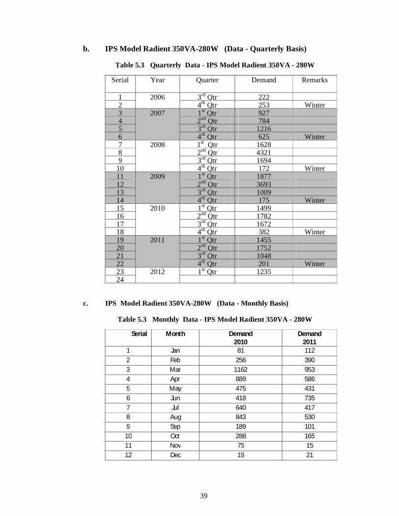
b. IPS Model Radient 350VA-280W (Data - Quarterly Basis)
Table 5.3 Quarterly Data - IPS Model Radient 350VA - 280W
Serial Year Quarter Demand Remarks
1 2006 3rd Qtr 222 2 4th Qtr 253 Winter 3 2007 1st Qtr 927 4 2nd Qtr 784 5 3rd Qtr 1216 6 4th Qtr 625 Winter 7 2008 1st Qtr 1628 8 2nd Qtr 4321 9 3rd Qtr 1694
10 4th Qtr 172 Winter 11 2009 1st Qtr 1877 12 2nd Qtr 3693 13 3rd Qtr 1009 14 4th Qtr 175 Winter 15 2010 1st Qtr 1499 16 2nd Qtr 1782 17 3rd Qtr 1672 18 4th Qtr 382 Winter 19 2011 1st Qtr 1455 20 2nd Qtr 1752 21 3rd Qtr 1048 22 4th Qtr 201 Winter 23 2012 1st Qtr 1235 24
c. IPS Model Radient 350VA-280W (Data - Monthly Basis)
Table 5.3 Monthly Data - IPS Model Radient 350VA - 280W
Serial Month Demand 2010
Demand 2011
1 Jan 81 112 2 Feb 256 390 3 Mar 1162 953 4 Apr 889 586 5 May 475 431 6 Jun 418 735 7 Jul 640 417 8 Aug 843 530 9 Sep 189 101
10 Oct 288 165 11 Nov 75 15 12 Dec 19 21
39

CHAPTER 6
FORECASTING MODEL DEVELOPMENT - INSTANT POWER SUPPLY (IPS) UNITS
6.1 Introduction
There are two general approaches to forecasting, just as there are two ways to tackle all decision
modeling. One is the quantitative analysis; the other is qualitative approach. Quantitative
forecasts use a variety of mathematical models that rely on historical data and/or casual variables
to forecast demand. Subjective or qualitative forecast incorporate such factors as the decision
maker’s intuition, emotion, personal experiences, and value system in reaching a forecast. Some
firms use one approach and some use the other. In practice, a combination of the two is usually
most effective.
In this study, out of collected data of various models of IPS, analysis will be carried out on IPS
Models - Compuve VLX 600 VA - 500Watt and Radient 350 VA – 280 Watt manufactured by
Rahimafrooz, using quantitative forecasting method. While developing forecasting, at first
yearly demand will be considered and since the demand of IPS varies with seasons in particular
more in summer and less in winter, so finally quarterly demand data will be used to find out the
seasonal effect. These models of IPS are chosen because they were introduced in the long
before and there was no discontinuity of the production of the products (models) for last eight
years. The forecasting result will be evaluated using forecasting error measurement - Mean
Absolute Deviation (MAD), Mean Squared Error (MSD), and Mean Absolute Percent Error
(MAPE) of these forecasting methods.
Selection Criteria of Market Demand Forecast Methods
When carrying out market demand forecast, one often confronts with the problem of the
inappropriate selection of a forecast method. It should be noted that in every actual forecast
situation methods have their advantages and disadvantages, hence, it is important to define and
analyse forecast method selection criteria. Despite the fact that there are a lot of different
forecast methods, the researchers define common assumptions for forecast method application
based on their accuracy. Firstly, most of the quantitative forecast methods are based on the
assumption that a certain reasonable linkage that existed in the past, will remain in the future.
Secondly, the forecast accuracy by using any forecast method gets reduced with the increase of
the forecast time span. In other words, long-term forecast is less reliable than the short-term one
due to the factors that cause potential uncertainty.
40

Thirdly, the forecast for the whole market demand is usually more accurate than the forecast for
a separate product because in the former case, the demand forecast errors for separate product
groups just eliminate each other (Herbig, Milewicz, Golden, 1994) [1].
The selection of the forecast method should be based at least on several criteria taking into
account forecast method applicability and additional things proposed by researchers such as:
• Forecast accuracy degree.
• Time span.
• Amount of necessary initial data.
• Forecast costs.
• Result implementation and applicability level
The priorities of forecast method application are determined according to the forecast time span
which is traditionally divided into short- (1-3 months), mid- (3months- 2 years) and long- (more
than two years). Simple quantitative forecast methods are applied for short- and mid- period of
time (simple moving average and exponential smoothing), while for long-term forecast
regression and econometric models are applied [1].
Research Methodology
The main objective of the research was to select a forecast method for the Instant Power Supply
(IPS) units demand manufactured by Rahimafrooz, Bangladesh. To develop the quantitative
forecast, the forecast methods were selected depending on the scope of information in hand
about the IPS market. Therefore, the methods of Naïve Approach, Simple Moving Average,
Weighted Moving Average, Regression and Seasonal Trend Analysis were carried out to
estimate demands.
In order to identify the most accurate forecast method, quite often ex post indicators are used in
the research literature. The main ex post indicators defining the forecast accuracy are Forecast
Error, Mean Absolute Deviation (MAD), Mean Squared Error (MSD), Mean Absolute Percent
Error (MAPE) of above mentioned forecasting methods.
41

6.4 Development of Demand Forecasting of IPS Models
The demann forecast of IPS models - Compuve VLX 600VA - 500W and Radient 350VA - 280W manufactured by Rahimafrooz will be first found out by applying Naïve Approach, Simple Moving Average, Weighted Moving Average, Regression and Seasonal Trend Analysis and then forecast accuracy assessment indicators forecast error , mean absolute percentage error MAPE, mean percentage error MPE and Mean squared error MSE will also be calculated. After comparison of error values calculated by using different forecast methods, the smallest difference between IPS sales forecast and fact; will discloses high forecast accuracy.
6.4.1 Technical Analysis on Data of IPS Model Compuve VLX 600VA - 500Watts
Yearly and quarterly market demand of Compuve VLX 600VA - 500W model of IPS was as following:
a. IPS - Model Compuve VLX 600 - 500 WATT, 2 HRS (Data - Yearly Basis)
Table 6.1 Yearly Demand IPS Compuve VLX 600 - 500 Watt
Year Demand, Di 2004-2005 2554 2005-2006 3836 2006-2007 8125 2007-2008 11501 2008-2009 10789 2009-2010 4664 2010-2011 5128 2011-2012 3493
b. IPS - Model Compuve VLX 600 - 500 WATT, 2 HRS (Data - Quarterly Basis) :
Table 6.2 Querterly Demand IPS Compuve VLX 600 - 500 Watt
Serial Year Quarter Quantity Sold Remarks 1 2006 3rd Qtr 2006 483 2 4th Qtr 2006 1404 Winter 3 2007 1st Qtr 2007 2187 4 2nd Qtr 2007 2543 5 3rd Qtr 2007 2042 6 4th Qtr 2007 1179 Winter 7 2008 1st Qtr 2008 2283 8 2nd Qtr 2008 5997 9 3rd Qtr 2008 2843
10 4th Qtr 2008 513 Winter 11 2009 1st Qtr 2009 2754 12 2nd Qtr 2009 4679 13 3rd Qtr 2009 1311 14 4th Qtr 2009 277 Winter 15 2010 1st Qtr 2010 1403 16 2nd Qtr 2010 1673 17 3rd Qtr 2010 1500
Serial Year Quarter Quantity Sold Remarks 18 4th Qtr 2010 442 Winter 19 2011 1st Qtr 2011 1602 20 2nd Qtr 2011 1584 21 3rd Qtr 2011 1252 22 4th Qtr 2011 288 Winter 23 2012 1st Qtr 2012 1589 24
42

Received yearly data will be used in above mentions forecasting methods and error of each method will be found out to get the most suited forecasting model. Finally quarterly data will be used to find out seasonal variations in data with trend analysis.
6.4.1.1 Naïve Approach
Table 6.3 Forecasted Demand and Errors by Naïve Approach
From the above table we observe that the MAD (Mean Absolute Deviation) , MAPE (Mean Absolute Percentage Error) and MSE are 2554.71 , 44.19% and 10,335,358.71 respectively.
Figure 6.1 Graph showing actual demand, forecast and deviation
From the above graph we can observe that around first half of the time the forecasted data was less than the demanded data and for the next half the forecasted data was more than the demand.
6.4.1.2 Moving Average:
43
Year Demand Di
Forecast Fi
Error Di-Fi |Di-Fi| APE (%) MAPE MAD
MSE
2004-2005 2554 - - - -
44.19 2554.71 10,335,358.71
2005-2006 3836 2554 1282 1282 33.42
2006-2007 8125 3836 4289 4289 52.79
2007-2008 11501 8125 3376 3376 29.35
2008-2009 10789 11501 -712 712 6.6
2009-2010 4664 10789 -6125 6125 131.33
2010-2011 5128 4664 464 464 9.05
2011-2012 3493 5128 -1635 1635 46.81

6.4.1.2.1 Simple Moving Average
Table 6.4 Forecasted Demand and Errors by Simple Moving Average
Year Demand Di
Forecast Fi
Error Di-Fi |Di-Fi| APE
(%) MAPE MAD
MSE
2004-2005 2554 15,545,408.96
3529.12 53.28
2005-2006 3836 2554 1282 1282 33.4 2006-2007 8125 3195 4930 4930 60.68 2007-2008 11501 4838.33 6662.67 6662.67 57.93 2008-2009 10789 6504 4285 4285 39.71 2009-2010 4664 7361 -2697 2697 57.83 2010-2011 5128 6811.5 -1683.5 1683.5 32.83
2011-2012 3493 6656.71 -3163.71 3163.71 90.57
From the above table we observe that the MAD, MSE and MAPE are 3529.12, 15,545, 408.96 and 53.28% respectively.
Figure 6.2 : Graph showing actual demand, forecast and deviation
From the above graph we can observe that around first two third of the time the forecasted data was less than the demanded data and for the last one third the forecasted data was more than the actual demand.
44

6.4.1.2.2 Weighted Average
a. Simple Weighted Average:
Table 6.5 Forecasted Demand and Errors by Simple Weighted Average
Year Demand Di Weight Forecast
Fi Error Di-Fi |Di-Fi| APE
(%)
MSE MAD MAPE
2004-2005 2554 1
14,641,502.23 3567.5 58.97
2005-2006 3836 2 2554 1282 1282 33.4
2006-2007 8125 3 3408.67 4716.33 4716.33 58.1
2007-2008 11501 4 5766.84 5734.16 5734.16 49.9
2008-2009 10789 5 8060.5 2728.5 2728.5 25.3
2009-2010 4664 6 8970 -4306 4306 92.3
2010-2011 5128 7 7739.71 -2611.71 2611.71 50.9
2011-2012 3493 8 7086.78 -3593.78 3593.78 103
From the above table we observe that the MAD, MSE and MAPE are 3567.5 , 14,641,502.23 and 58.97% respectively.
Figure 6.3 Graph showing actual demand, forecast and deviation
From the above graph we can observe that around two third of the time the forecasted data was less than the demanded data and for the last one third time the forecasted data was more than the actual demand.
45

b. 2 Years Weighted Average
Table 6.6 Forecasted Demand and Errors by 2 Years Weighted Average
Year Demand Di
Forecast Fi
Error Di-Fi |Di-Fi| APE
(%)
MSE
MAD MAPE
2004-2005 2554
7,588,406.62
3225.94
52.2
2005-2006 3836 2006-2007 8125 3408.67 4716.33 4716.33 58.05 2007-2008 11501 6695.33 4805.67 4805.67 41.78 2008-2009 10789 10375.67 413.33 413.33 3.83 2009-2010 4664 11026.33 -6362.33 6362.33 136.41 2010-2011
5128 6705.67 -1577.67 1577.67 30.77 2011-2012
3493 4973.33 -1480.33 1480.33 42.38
From the above table we observe that the MAD, MSE and MAPE are 3225.94, 7,588,406.62 and 52.20 % respectively.
Figure 6.4 Graph showing actual demand, forecast and deviation
From the above graph we can observe that around first half of the time the forecasted data was less than the demanded data and for the next half the forecasted data was more than the actual demand.
46

c. 3 Years Weighted Average
Table 6.7 Forecasted Demand and Errors by 3 Years Weighted Average
Year Demand Di
Forecast Fi Di-Fi |Di-Fi| APE
(%)
MSE MAD MAPE
2004-2005 2554
16,811,724.07 3697 62.96
2005-2006 3836
2006-2007 8125
2007-2008 11501 5766.83 5734.17 5734.17 49.86
2008-2009 10789 9098.17 1690.83 1690.83 15.67
2009-2010 4664 10582.33 -5918.33 5918.33 126.89
2010-2011 5128 7845.17 -2717.17 2717.17 52.99
2011-2012 3493 5916.83 -2423.83 2423.83 69.39
From the above table we observe that the MAD, MSE and MAPE are 3696, 16,811,724.07 and 62.96 % respectively.
Figure 6.5 Graph showing actual demand, forecast and deviation
From the above graph we can observe that around first one third of the time the forecasted data was less than the demanded data and for the next two third time the forecasted data was more than the demand.
47

d. 4 Years Weighted Average
Table 6.8 Forecasted Demand and Errors by 4 Years Weighted Average
Year Demand Di
Forecast Fi
Error Di-Fi |Di-Fi| APE
(%)
MSE MAD MAPE
2004-2005 2554
13,438,418.90
3547.83
72.14
2005-2006 3836
2006-2007 8125
2007-2008 11501
2008-2009 10789 8060.5 2728.5 2728.5 25.29
2009-2010 4664 9774.5 -5110.5 5110.5 109.57
2010-2011 5128 8215 -3087 3087 60.2
2011-2012 3493 6758.3 -3265.3 3265.3 93.48
From the above table we observe that the MAD and MAPE are 3547.83, 13,438,418.90 and 72.14 % respectively.
Figure 6.6 Graph showing actual demand, forecast and deviation
From the above graph we can observe that around almost all the forecasted period the forecasted data was more than the demanded data.
48

6.4.1.3 Exponential Smoothing Method
As this IPS is a new product in Bangladesh we are considering the coefficient of deviation, = 0.8
Table 6.9 Forecasted Demand and Errors by Exponential Smoothing Method
Year Demand Di
Forecast Fi
Eorrr Di-Fi |Di-Fi| APE
(%)
MSE MAD MAPE
2004-2005 2554 0
11,658,375.89
2699
46.4
2005-2006 3836 2554 1282 1282 33
2006-2007 8125 3580 4545.4 4545.4 56
2007-2008 11501 7216 4285.1 4285.1 37
2008-2009 10789 10644 145 145 1.3
2009-2010 4664 10760 -6096 6096 131
2010-2011 5128 5883 -755.2 755.2 15
2011-2012 3493 5279 -1786 1786 51
From the above table we observe that the MAD, MSE and MAPE are 2699, 11,658,375.89 and 46.4% respectively.
Figure 6.7 Graph showing actual demand, forecast and deviation
From the above graph we can observe that around first half of the time the forecasted data was less than the demanded data and for the next half the forecasted data was more than actual demand.
49

6.4.1.4 Trend Analysis
Table 6.10 Yearly Data for Trend Analysis
Year Time Period (x)
Demand (Y)
∑x X2 xy
2004-2005 1 2554 1 1 2554 2005-2006 2 3836 2 4 7672 2006-2007 3 8125 3 9 24375 2007-2008 4 11501 4 16 46004 2008-2009 5 10789 5 25 53945 2009-2010 6 4664 6 36 27984 2010-2011 7 5128 7 49 35896 2011-2012 8 3493 8 64 27944
∑y= 50090 ∑x= 36 ∑x2 = 20204204 ∑xy=226374
Average x = 4.5 Average y = 6261.25, b= 23.07
∑ xy - n (Avg x) (Avg y ) b = ---------------------------
∑ x2 - n (Avg x)2 Where b = slope of the regression line
∑ = summation sign, x = known values of the independent variables
y = known values of the dependent variables, Avg x = average of the x – values
Avg y = average of the y – values, n = number of data point or observations
y – intercept can be computed as follows:
a = y – bx , a = 6261.25- 23.07x4.5 = 6157.435
y = a + bx, y1= 6157.435+23.07x1 = 6180.5
Table 6.11 Showing Forecasted Demand and Errors by Trend Analysis
Year Demand Di
Forecast Fi
Eorrr Di-Fi |Di-Fi| APE
(%)
MSE MAD MAPE
2004-2005 2554 6180.5 -3626.5 3626.5 141.99
10,316,342.87 2916.46 56.8
2005-2006 3836 6203.57 -2367.57 2367.57 61.72
2006-2007 8125 6226.64 1898.35 1898.35 23.36
2007-2008 11501 6249.71 5251.28 5251.28 45.66
2008-2009 10789 6272.78 4516.21 4516.21 41.86
2009-2010 4664 6295.85 -1631.86 1631.85 34.99
2010-2011 5128 6318.92 -1190.93 1190.92 23.22
2011-2012 3493 6342 -2849 2849 81.56
50

Figure 6.8 Graph showing actual demand Di, forecast Fi and deviation Di-Fi
From the above table we observe that the MAD, MSE and MAPE are 2916.46, 10,316,342.87 and 56.80 % respectively.
6.4.1.5 Seasonal Trend
Table 6.11 Showing Forecasted Demand and Errors by Seasonal Trend Analysis
Year Quarter Demand Di
Forecast Fi
Eorrr Di-Fi |Di-Fi| APE (%)
MSE
MAD MAPE
2006 3rd Qtr 483 2041.83 -1558.84 1558.84 322.74
750847.65 619.58 47.71
4th Qtr 1404 869.72 534.27 534.28 38.05
2007 1st Qtr 2187 2451.54 -264.54 264.54 12.1
2nd Qtr 2543 4011.79 -1468.79 1468.79 57.76
3rd Qtr 2042 1870.92 171.07 171.07 8.38
4th Qtr 1179 795.36 383.63 383.63 32.54
2008 1st Qtr 2283 2237.37 45.62 45.62 2
2nd Qtr 5997 3653.49 2343.50 2343.5 39.08
3rd Qtr 2843 1700.016 1142.984 1142.98 40.2
4th Qtr 513 721.0109 -208.011 208.011 40.55
2009 1st Qtr 2754 2023.208 730.7916 730.792 26.54
2nd Qtr 4679 3295.199 1383.801 1383.8 29.57
3rd Qtr 1311 1529.105 -218.105 218.105 16.64
4th Qtr 277 646.6555 -369.656 369.656 133.45
2010 1st Qtr 1403 1809.04 -406.04 406.04 28.94
2nd Qtr 1673 2936.902 -1263.9 1263.9 75.55
3rd Qtr 1500 1358.195 141.8051 141.805 9.45
4th Qtr 442 572.3001 -130.3 130.3 29.48
2011 1st Qtr 1602 1594.872 7.128041 7.12804 0.44
2nd Qtr 1584 2578.604 -994.604 994.604 62.79
3rd Qtr 1252 1187.284 64.71559 64.7156 5.17
4th Qtr 288 497.9447 -209.945 209.945 72.9
2012 1st Qtr 1589 1380.704 208.2963 208.296 13.11
From the above table we observe that the MAD, MSE and MAPE are 750847.65, 619.58 and 47.71.
51

Figure 6.9 Graph showing actual demand, forecast and deviation
From the above graph we can observe that other than 1st, 4th, 16th and 20th quarters, in all other quarters deviations are very less.
6.4.1.6. Summary of Forecasting Errors
Table 6.12 Showing Summary of Forecasting Errors by Various Methods
Name of the methods MAD MAPE (%)
Naïve Approach 2554.71 44.19
Exponential Smoothing 2699
46.4
Simple Moving Average 3529.12 53.28
Simple weighted average 3567.5 58.97
2 years weighted average 3225.94
52.2
3 years weighted average 3697 62.96
4 years weighted average 3547.83
72.14
Trend analysis 2916.46 56.8
Seasonal trend 619.58 47.71
From the above table we can see that seasonal trend analysis has the minimum MAD and 2nd lowest MAPE.
So, we can deduce that for Compuve VLX 600VA-500W IPS, Seasonal Trend Analysis gives the minimum error.
52

6.4.2 Technical Analysis on Data of IPS Model Radient 350VA-280W
Yearly and quarterly market demand of IPS Model Radient 350VA-280W was as following:
a. IPS Model Radient 350VA-280W (Data - Yearly Basis) :
Table 6.13 Yearly Demand IPS IPS Model Radient 350VA-280 Watt
Year Demand
2005-2006 1011 2006-2007 2186 2007-2008 7790 2008-2009 7436 2009-2010 4465 2010-2011 2314 2011-2012 3389
b. IPS Model Radient 350VA-280W (Data - Quarterly Basis) :
Table 6.14 Quarterly Demand IPS IPS Model Radient 350VA-280 Watt
Serial Year Quarter Demand Remarks 1 2006 3rd Qtr 222 2 4th Qtr 253 Winter 3 2007 1st Qtr 927 4 2nd Qtr 784 5 3rd Qtr 1216 6 4th Qtr 625 Winter 7 2008 1st Qtr 1628 8 2nd Qtr 4321 9 3rd Qtr 1694 10 4th Qtr 172 Winter 11 2009 1st Qtr 1877 12 2nd Qtr 3693 13 3rd Qtr 1009 14 4th Qtr 175 Winter 15 2010 1st Qtr 1499 16 2nd Qtr 1782 17 3rd Qtr 1672 18 4th Qtr 382 Winter 19 2011 1st Qtr 1455 20 2nd Qtr 1752 21 3rd Qtr 1048 22 4th Qtr 201 Winter 23 2012 1st Qtr 1235 24
Received yearly data will be used in various forecasting methods and quarterly data will be used to find out seasonal variations in data with trend analysis.
53

6.4.2.1 Naïve Approach
Table 6.15 Showing Forecasted Demand and Errors by Naïve Approach
Years Demand Di
Forecast Fi
Eorrr Di-Fi |Di-Fi| APE
(%) MSE MAD MAPE
2005-2006 1011
5974424.078
2221.67 53.61
2006-2007 2186 1011 1175 1175 53.75
2007-2008 7790 2186 5604 5604 71.94
2008-2009 7436 7790 -354 354 4.76
2009-2010 4465 7436 -2971 2971 66.54
2010-2011 2314 4465 -2151 2151 92.96
2011-2012 3389 2314 1075 1075 31.72
From the above table we observe that the MAD (Mean Absolute Deviation), MSE (Mean Squared Error) and MAPE (Mean Absolute Percentage Error) are 2221.67, 5974424.078 and 53.61% respectively.
Figure 6.10 : Graph showing actual demand, forecast and deviation
From the above graph we can observe that around first half of the time the forecasted data was less than the demanded data and for the next half the forecasted data was more than actual demand.
54

6.4.2.2 Weighted Average:
a. Simple weighted average:
Table 6.16 Showing Forecasted Demand and Errors by Simple weighted average Method
Years Dema
nd Di
Weight Forecast Fi
Error Di-Fi |Di-Fi| APE
(%)
MSE MAD MAPE
2005-2006 1011 1
9490400 2565.69 60.53
2006-2007 2186 2 1011 1175 1175 53.75
2007-2008 7790 3 1794.3 5995.67 5995.7 76.97
2008-2009 7436 4 4792.2 2643.83 2643.8 35.55
2009-2010 4465 5 5849.7 -1384.7 1384.7 31.01
2010-2011 2314 6 5388.1 -
3074.13
3074.1 132.85
2011-2012 3389 7 4509.8 -1120.8 1120.8 33.07
From the above table we observe that the MAD and MAPE are 2565.69, 9490400 and 60.53%.
Figure 6.12 Graph showing actual demand, forecast and deviation
From the above graph we can observe that around first half of the time the forecasted data was less than the demanded data. And for the next half the forecasted data was less.
55

b. 2 Years Weighted Average
Table 6.17 Showing Forecasted Demand and Errors by 2 Years Weighted Average
Years Demand Di
Forecast Fi
Error Di-Fi |Di-Fi| APE
(%)
MSE MAD MAPE
2005-2006 1011
11555693 2819.6 62.56
2006-2007 2186
2007-2008 7790 1794.33 5995.67 5995.7 76.97
2008-2009 7436 5922 1514 1514 20.36
2009-2010 4465 7554 -3089 3089 69.18
2010-2011 2314 5455.33 -3141.3 3141.3 135.75
2011-2012 3389 3031 358 358 10.56
From the above table we observe that the MAD (Mean Absolute Deviation) and MAPE (Mean Absolute Percentage Error) are 2819.6, 11555693 and 62.56
Figure 6.13 Graph showing actual demand, forecast and deviation
From the above graph we can observe that around first half of the time the forecasted data was less than the demanded data and for the next half the forecasted data was more than the demand.
56

c. 3 Years Weighted Average:
Table 6.18 Showing Forecasted Demand and Errors by 3 Years Weighted Average Method
Years Demand Di
Forecast Fi
Error Di-Fi |Di-Fi| APE
(%)
MSE MAD MAPE
2004-2005 1011
6448511
2262.25
64.87
2005-2006 2186
2006-2007 7790
2007-2008 7436 4792.17 2643.83 2643.83 35.55
2008-2009 4465 6679 -2214 2214 49.59
2009-2010 2314 6009.5 -3695.5 3695.5 159.7
2010-2011 3389 3884.67 -495.67 495.67 14.63
From the above table we observe that the MAD, MSE and MAPE are 2262.25, 6448511 and 64.87.
Figure: 14 Graph showing actual demand, forecast and deviation
From the above graph we can observe that for most of the time the forecasted data was more than the demanded data.
57

d. 4 Years Weighted Average
Table 6.19 Forecasted Demand and Errors by 4 Years Weighted Average Method
Year Demand Di
Forecast Fi
Eorrr Di-Fi |Di-Fi| APE
(%)
MSE MAD MAPE
2005-2006 1011
24706.11 2002.13 71.69
2006-2007 2186
2007-2008 7790
2008-2009 7436
2009-2010 4465 5849.7 -1384.7 1384.7 31.01
2010-2011 2314 5793.4 -3479.4 3479.4 150.36
2011-2012 3389 4531.3 -1142.3 1142.3 33.71
From the above table we observe that the MAD (Mean Absolute Deviation) and MAPE (Mean Absolute Percentage Error) are 2002.13, 24706.1 and 71.69 %.
Figure 6.15 Graph showing actual demand, forecast and deviation
From the above graph we can observe that for most of the time the forecasted data was more than the demanded data.
58

6.4.2.3 Exponential Smoothing
As this IPS is a new product in Bangladesh we are considering the coefficient of deviation, = 0.8
Table 6.20 Showing Forecasted Demand and Errors by Exponential Smoothing Method
From the above table we observe that the MAD, MSE and MAPE are 2313.52, 8610760 and 56.
Figure 6. 11 Graph showing actual demand, forecast and deviation
From the above graph we can observe that around first half of the time the forecasted data was less than the demanded data and for the next half the forecasted data was more than the demand.
59
Year Demand Di
Forecast Fi
Eorrr Di-Fi |Di-Fi| APE
(%)
MSE
MAD MAPE
2005-2006 1011
8610760
2313.52 56
2006-2007 2186 1011 1175 1175 53.75
2007-2008 7790 1951 5839 5839 74.96
2008-2009 7436 6622.2 813.8 813.8 10.94
2009-2010 4465 7273.2 -2808.2 2808.2 62.89
2010-2011 2314 5026.6 -2712.6 2712.6 117.23
2011-2012 3389 2856.5 532.5 532.5 15.71

6.4.2.4 Trend Analysis
Table 6.21 Showing Forecasted Demand and Errors by Trend Analysis
Year Demand Di
Forecast Fi
Eorrr Di-Fi |Di-Fi| APE(%)
MSE MAD MAPE
2005-2006 1011 3648.893 -2637.89 2637.89 260.92
5883849
2125.06 79.53
2006-2007 2186 3794.071 -1608.07 1608.07 73.56
2007-2008 7790 3939.25 3850.75 3850.75 49.43
2008-2009 7436 4084.42 3351.57 3351.57 45.07
2009-2010 4465 4229.6 235.39 235.39 5.27
2010-2011 2314 4374.78 -2060.79 2060.78 89.06
2011-2012 3389 4519.96 -1130.96 1130.96 33.37
From the above table we observe that the MAD, MSE and MAPE are 2125.06, 5883849and 79.53%.
Figure 6.16 Graph showing actual demand, forecast and deviation
From the above graph we can observe that around half of the time the forecasted data was less than the demanded data and for the rest half the forecasted data was more than the demanded data.
60

6.4.2.5 Seasonal Trend (Quarterly Data)
Table 6.22 Showing Forecasted Demand and Errors by Seasonal Trend Analysis
Period Year Demand Di
Forecast Fi
Eorrr Di-Fi
|Di-Fi| APE (%)
MSE MAD MAPE
1 2006 222 1063.51 -841.51 841.51 379.06
581221.6
591.09 92.1
2 Winter 253 282.17 -29.17 29.17 11.53
3 2007 927 1354.60 -427.60 427.60 46.13
4 784 2340.93 -1556.93 1556.93 198.59
5 1216 1501.86 -285.86 285.86 23.51
6 Winter 625 657.74 -32.74 32.74 5.24
7 2008 1628 1907.04 -279.04 279.04 17.14
8 4321 3211.38 1109.61 1109.61 25.68
9 1694 1541.84 152.15 152.15 8.98
10 Winter 172 675.13 -503.13 503.13 292.52
11 2009 1877 1957.14 -80.14 80.14 4.27
12 3693 3295.19 397.80 397.80 10.77
13 1009 1581.82 -572.82 572.82 56.77
14 Winter 175 692.53 -517.53 517.53 295.73
15 2010 1499 2007.24 -508.24 508.24 33.91
16 1782 3379.01 -1597.01 1597.01 89.62
17 1672 1621.80 50.19 50.19 3
18 Winter 382 709.92 -327.92 327.92 85.84
19 2011 1455 2057.34 -602.34 602.34 41.4
20 1752 3462.83 -1710.83 1710.83 97.65
21 1048 1661.78 -613.78 613.78 58.57
22 Winter 201 727.31 -526.31 526.31 261.85
23 2012 1235 2107.44 -872.44 872.44 70.64
From the above table we observe that the MAD, MSE and MAPE are 591.09, 581221.6 and 92.1%.
61

Figure 6. 17 Graph showing actual demand, forecast and deviation
From the above graph we can observe that other than 2nd quarters in all other quarters deviations are very less.
6.4.2.7. Summary of forecasting errors
Name of the methods MAD MAPE (%)
Naïve 2221.67 53.61
Exponential 2313.52
56
Simple weighted average 2565.69 60.53
2 years weighted average 2819.6
62.53
3 years weighted average 2262.25 64.87
4 years weighted average 2002.13
71.69
Trend analysis 2125.06 79.53
Seasonal trend 591.09 92.1
Season Trend With 12 Recent Quarters Data 51.52 38.35
62
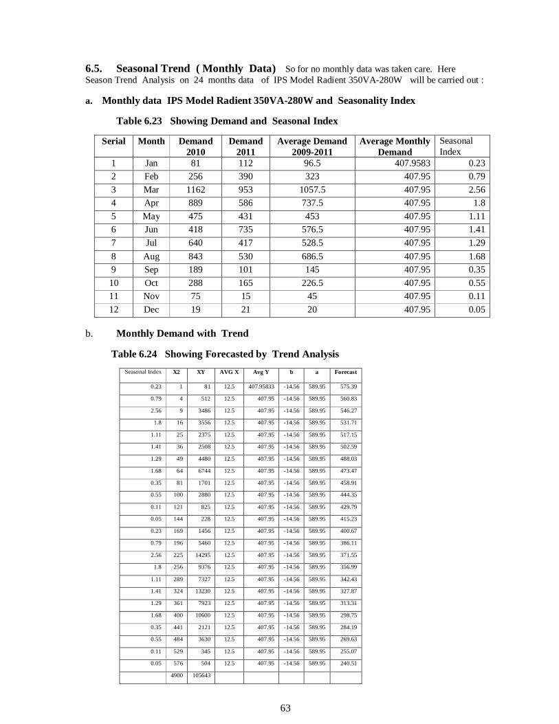
6.5. Seasonal Trend ( Monthly Data) So for no monthly data was taken care. Here Season Trend Analysis on 24 months data of IPS Model Radient 350VA-280W will be carried out :
a. Monthly data IPS Model Radient 350VA-280W and Seasonality Index
Table 6.23 Showing Demand and Seasonal Index
Serial Month Demand 2010
Demand 2011
Average Demand 2009-2011
Average Monthly Demand
Seasonal Index
1 Jan 81 112 96.5 407.9583 0.23 2 Feb 256 390 323 407.95 0.79 3 Mar 1162 953 1057.5 407.95 2.56 4 Apr 889 586 737.5 407.95 1.8 5 May 475 431 453 407.95 1.11 6 Jun 418 735 576.5 407.95 1.41 7 Jul 640 417 528.5 407.95 1.29 8 Aug 843 530 686.5 407.95 1.68 9 Sep 189 101 145 407.95 0.35 10 Oct 288 165 226.5 407.95 0.55 11 Nov 75 15 45 407.95 0.11 12 Dec 19 21 20 407.95 0.05
b. Monthly Demand with Trend
Table 6.24 Showing Forecasted by Trend Analysis Seasonal Index X2 XY AVG X Avg Y b a Forecast
0.23 1 81 12.5 407.95833 -14.56 589.95 575.39
0.79 4 512 12.5 407.95 -14.56 589.95 560.83
2.56 9 3486 12.5 407.95 -14.56 589.95 546.27
1.8 16 3556 12.5 407.95 -14.56 589.95 531.71
1.11 25 2375 12.5 407.95 -14.56 589.95 517.15
1.41 36 2508 12.5 407.95 -14.56 589.95 502.59
1.29 49 4480 12.5 407.95 -14.56 589.95 488.03
1.68 64 6744 12.5 407.95 -14.56 589.95 473.47
0.35 81 1701 12.5 407.95 -14.56 589.95 458.91
0.55 100 2880 12.5 407.95 -14.56 589.95 444.35
0.11 121 825 12.5 407.95 -14.56 589.95 429.79
0.05 144 228 12.5 407.95 -14.56 589.95 415.23
0.23 169 1456 12.5 407.95 -14.56 589.95 400.67
0.79 196 5460 12.5 407.95 -14.56 589.95 386.11
2.56 225 14295 12.5 407.95 -14.56 589.95 371.55
1.8 256 9376 12.5 407.95 -14.56 589.95 356.99
1.11 289 7327 12.5 407.95 -14.56 589.95 342.43
1.41 324 13230 12.5 407.95 -14.56 589.95 327.87
1.29 361 7923 12.5 407.95 -14.56 589.95 313.31
1.68 400 10600 12.5 407.95 -14.56 589.95 298.75
0.35 441 2121 12.5 407.95 -14.56 589.95 284.19
0.55 484 3630 12.5 407.95 -14.56 589.95 269.63
0.11 529 345 12.5 407.95 -14.56 589.95 255.07
0.05 576 504 12.5 407.95 -14.56 589.95 240.51
4900 105643
63
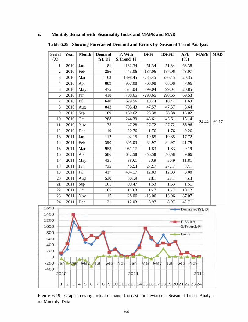
c. Monthly demand with Seasonality Index and MAPE and MAD
Table 6.25 Showing Forecasted Demand and Errors by Seasonal Trend Analysis
Serial (X)
Year Month Demand (Y), Di
F. With S.Trend, Fi
Di-Fi IDi-FiI APE (%)
MAPE MAD
1 2010 Jan 81 132.34 -51.34 51.34 63.38
24.44
69.17
2 2010 Feb 256 443.06 -187.06 187.06 73.07 3 2010 Mar 1162 1398.45 -236.45 236.45 20.35 4 2010 Apr 889 957.08 -68.08 68.08 7.66 5 2010 May 475 574.04 -99.04 99.04 20.85 6 2010 Jun 418 708.65 -290.65 290.65 69.53 7 2010 Jul 640 629.56 10.44 10.44 1.63 8 2010 Aug 843 795.43 47.57 47.57 5.64 9 2010 Sep 189 160.62 28.38 28.38 15.02
10 2010 Oct 288 244.39 43.61 43.61 15.14 11 2010 Nov 75 47.28 27.72 27.72 36.96 12 2010 Dec 19 20.76 -1.76 1.76 9.26 13 2011 Jan 112 92.15 19.85 19.85 17.72 14 2011 Feb 390 305.03 84.97 84.97 21.79 15 2011 Mar 953 951.17 1.83 1.83 0.19 16 2011 Apr 586 642.58 -56.58 56.58 9.66 17 2011 May 431 380.1 50.9 50.9 11.81 18 2011 Jun 735 462.3 272.7 272.7 37.1 19 2011 Jul 417 404.17 12.83 12.83 3.08 20 2011 Aug 530 501.9 28.1 28.1 5.3 21 2011 Sep 101 99.47 1.53 1.53 1.51 22 2011 Oct 165 148.3 16.7 16.7 10.12 23 2011 Nov 15 28.06 -13.06 13.06 87.07 24 2011 Dec 21 12.03 8.97 8.97 42.71
Figure 6.19 Graph showing actual demand, forecast and deviation - Seasonal Trend Analysis on Monthly Data
64

6.6 Summary of Forecasting Errors
Name of the methods MAD MAPE (%)
Naïve 2221.67 53.61
Exponential 2313.52
56
Simple weighted average 2565.69 60.53
2 years weighted average 2819.6
62.53
3 years weighted average 2262.25 64.87
4 years weighted average 2002.13
71.69
Trend analysis 2125.06 79.53 Seasonal trend With 12 Recent Quarters Data 591.09 92.1
Season Trend With 36 Recent Months Data
69.17 24.44
From the above table we can see that Seasonal Trend Analysis in particular monthly data gives the minimum MAD and MAPE. So, we can deduce that for Radient 350VA-280W IPS seasonal trend analysis gives the minimum error.
From the above analysis we have found that Seasonal Trend Analysis is most suitable for market demand forecasting of IPS manufactured by Rahimafrooz. It was also found that monthly data gives less error in forecasting than quarterly data.
65

CHAPTER 7
CONCLUSION AND RECOMMENDATION
7.1. Conclusion
Forecast method classification should be based on availability of information; period for which
the forecast is developed; forecast object; and forecast goal. The selection of the forecast
method should be based on several criteria taking into account the applicability of the forecast
method for market demand forecast, like forecast accuracy level, period, the scope of initial data,
forecast costs, and the level of result application and implementation.
The comparison of forecast accuracy assessment indicators estimated by using different forecast
methods identified that the minimum forecast error values were received by applying the
Seasonal Trend Analysis method where MAD = 69.17 and MAPE = 24.44 % . This MAD and
MAPE can be reduced more if we use yearly data and also use judgment in case forecasting
summer and winter months demands.
Demand forecasting allows manufacturers to make better decisions about which products to
promote to achieve objectives. By combining qualitative and quantitative forecast and common
sense we can increase our accuracy on forecast, because there are many situations where only
quantitative forecast is not enough to predict the market. In turn, this will reduce the cost of
inventory and minimize the chances of out of stocks.
7.2 Recommendations Following recommendations are brought out from this case study
a Forecasting methods should use data on actual behaviour, rather than judgments or
intentions, to predict behaviour.
b Methods that integrate judgmental and statistical data and procedures can improve
forecast accuracy in many situations.
c. Though simple methods have proven to be more accurate than relatively complex
methods. But products which are highly seasonal require complex methods, though their added cost and the reduced understanding among users, highly complex procedures need to be adopted.
66

REFERENCES
1) Haizer, J. and Render, B.,“ Operation Management” 8th edition, Pearson Education,
Inc.USA, 2007.
2) Chase, R. B., Aquilano, N. J. and Jacobs, F. R.,“ Production and Operations
Management” 8th edition, McGraw Hill Companies, Inc, USA, 1999.
3) Automotive and Electric Division (AED) Handbook, Rahimafrooz, Dhaka, 2010.
4) Michis, A. A., “Forecasting brand sales with wavelet decompositions of related causal
series”, International Journal of Business Forecasting and Marketing Intelligence, Vol. 1,
No. 2, pp. 95-110, 2009.
5) Savio, N. D., Nikolopoulos, K. and Bozos, K., “Improving the forecasting function for a
credit hire operator in the UK”, International Journal of Business Forecasting and
Marketing Intelligence, Vol. 1, No. 2, pp. 134-138, 2009.
6) Kanagasabapathi, B., Raj, K. A. D., Babu, B. S. and Shah, M., “Forecasting volumes for
trade promotions in CPG industry using market drivers”, International Journal of
Business Forecasting and Marketing Intelligence, Vol. 1, No. 2, pp. 139-152, 2009.
7) Anulark Pinnoib and Amnaj Charoenthavornyingb, “Demand Forecasting and
Production Planning for Highly Seasonal Demand Situations: Case Study of a Pressure
Container Factory Pisal Yenradeea,” 2001.
8) Pisal Yenradeea, Anulark Pinnoib and Amnaj Charoenthavornyingb, “Demand
Forecasting and Production Planning for Highly Seasonal Demand Situations:Case Study of
a Pressure Container Factory” ScienceAsia 27, pp. 271-278, 2001.
9) Hoi-Yin Cecilia Lai, “ Promotion demand forecast: A Case Study of Coca Cola
Enterprise” University of Nottingham, A Dissertation presented in part consideration for the
degree of MSc Operations Management,2007.
67

10) Pisal Yenradeea, Anulark Pinnoib and Amnaj Charoenthavornyingb, “Demand
Forecasting and Production Planning for Highly Seasonal Demand Situations:Case Study of
a Pressure Container Factory” ScienceAsia 27, pp. 271-278, 2001.
11) Armstrong, J.S., Morwitz, V.G. and Kumar, “Sales Forecasts for Existing Consumer
Products and Services: Do Purchase Intentions Contribute to Accuracy?” International
Journal of Forecasting. Vol. 16(3). pp. 383-397, 2000.
12) Wade G. Boudreaux , “Forecasting demand vs. forecasting "demand" ” UIRK’S
Marketing Research Review, Article ID: 20020202, February 2002.
13) M. Ahsan Akhtar Hasin, Shuvo Ghosh, and Mahmud A. Shareef, “An ANN
Approach to Demand Forecasting in Retail Trade in Bangladesh”, International Journal of
Trade, Economics and Finance, Vol. 2, No. 2, April 2011
14) J. Scott Armstrong, Kesten C. Green, Christopher R. Thomas and William F. Shughart
II (Eds.) “DEMAND FORECASTING: EVIDENCE-BASED METHODS” A chapter for
the forthcoming book Strategic Marketing M.anagement: A Business Process Approach, 17-
August- 2011.
15) Michael J. Baker (Ed.), “ SALES FORECASTING” Published in The IEBM
Encyclopedia of Marketing, International Thompson Business Press, pp. 278-290. 1999,]
16) Abdul Talib Bon, Chong Yi Leng, “The Fundamental on Demand Forecasting in
Inventory Management” Australian Journal of Basic and Applied Sciences, ISSN 1991-
8178, 3(4): pp. 3937-3943, 2009.
17) Vaida Pilinkienė, “Selection of Market Demand Forecast Methods: Criteria and
Application” ISSN 1392-2785 ENGINEERING ECONOMICS. No 3 (58), Kauno
technologijos universitetas K. Donelaičio g. 73, LT-44029, Kaunas 2008.
68

ANNEXURE A MARKET DEMAD DATA OF IPS 2004 - 2012
Table 5.1: Market Demand of IPS 2004-2005
2004-2005
Item 04-Jul 04-Aug 04-Sep 04-Oct 04-Nov 04-Dec 05-Jan 05-Feb 05-Mar
05-Apr 05-May
05-Jun Total
Category : IPS C/UNIT
IPS CONTROL UNIT B.CAT- 2 KVA 1 3 1 5
IPS C/UNIT RADIANT -350 VA 31 5 6 2 29 107 104 37 132 453
IPS C/UNIT IPS SUPREME-400 VA 2 1 1 4
IPS C/UNIT IPS SUPREME-600 VA 2 1 2 1 2 1 3 12
IPS C/UNIT COMPUVERTER-1400 VA 2 2 5 5 3 5 22
IPS C/UNIT POWER PLUS -750 VA 2 1 3
IPS C/UNIT COMPUVERTER-600 VA 2 1 1 3 7
IPS RADIANT 350VA - 280W 2HRS. 17 1 11 31 17 9 19 105
IPS SUPREME 400VA - 320W 3HRS. 43 49 39 40 10 8 6 57 137 104 107 203 803
IPS SUPREME 600VA - 500W 2HRS. 96 114 158 148 25 39 20 176 396 354 342 686 2554
IPS COMPUVE 600VA-500W 2HRS. 4 5 4 4 1 3 3 13 23 23 16 48 147
IPS POWER PLUS 750VA-600W 2HR. 8 14 16 6 3 1 4 11 40 22 12 71 208
IPS COMPUVE 1250VA-1000W 2HRS. 8 1 2 1 12
IPS COMPUVE 1400VA-1120W 2HRS. 12 32 43 42 15 11 16 40 70 90 47 106 524
IPS BLACK CAT 2.00 KVA-2HRS. 6 5 4 6 2 3 3 5 8 9 8 14 73
IPS CONTROL UNIT 1500G-1200W 3 11 17 9 5 4 2 8 22 28 23 59 191
IPS CONTROL UNIT 1000 JET-800W 8 4 12 23 8 1 13 10 29 30 23 161
IPS CONTROL UNIT 350G-300W 0 1 1
IPS CONTROL UNIT 350JET-300W 1 1
IPS 1500G-1200W 2HRS. 2 3 4 2 1 5 1 2 5 25
IPS 1500G-1200W 1HR. 5 6 11 16 12 9 17 22 20 14 15 147
IPS 1000G-800W 2HRS. 0 0
IPS 1000 JET-800W 2HRS. 23 9 16 17 15 7 21 37 41 30 17 233
Grand Total For IPS 221 256 324 363 91 99 72 404 914 855 682 141
0 5691
69
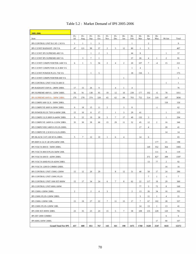
Table 5.2 : Market Demand of IPS 2005-2006
2005-2006
Item 05-Jul
05-Aug
05-Sep
05-Oct
05-Nov
05-Dec
06-Jan
06-Feb
06-Mar
06-Apr
06-May 06-Jun Total
IPS CONTROL UNIT B.CAT- 2 KVA 1 1 1 3 1 2 9
IPS C/UNIT RADIANT -350 VA 47 121 99 37 2 5 12 80 1 3 407
IPS C/UNIT IPS SUPREME-400 VA 1 2 1 44 8 1 57
IPS C/UNIT IPS SUPREME-600 VA 3 7 1 37 26 4 1 2 81
IPS C/UNIT COMPUVERTER-1400 VA 6 1 5 56 2 4 2 20 107 7 -4 15 221
IPS C/UNIT COMPUVER GLX-800 VA 1 4 5
IPS C/UNIT POWER PLUS -750 VA 1 5 18 150 1 175
IPS C/UNIT COMPUVERTER-600 VA 1 1
IPS CONTROL UNIT VOLTA 600 D 1 1
IPS RADIANT 350VA - 280W 2HRS. 17 15 26 9 4 1 4 76
IPS SUPREME 400VA - 320W 3HRS. 56 91 138 95 19 12 10 239 177 102 -6 78 1011
IPS SUPREME 600VA - 500W 2HRS. 170 278 374 328 65 62 84 703 752 514 319 187 3836
IPS COMPU 600 GLX - 500W 2HRS. 150 150
IPS COMPUVE 600VA-500W 2HRS. 6 18 15 11 2 3 8 -1 62
IPS POWER PLUS 750VA-600W 2HR. 15 10 8 17 1 3 29 41 1 125
IPS COMPU GLX 800VA-640W 2HRS. 9 22 19 30 5 7 17 49 132 3 1 294
IPS COMPUVE 1400VA-1120W 2HRS. 35 30 39 60 15 29 11 52 45 12 2 16 346
IPS COMPUVER 1400VA PLUS-2HRS. 17 4 20 41
IPS COMPUVE 2.50 KVA GLX-2HRS. 14 14
IPS BLACK CAT 2.00 KVA-2HRS. 5 7 12 10 1 6 4 14 6 65
IPS 800VA GLX LB UPS-640W 2HR. 177 21 198
IPS VOLTA 800 D - 560W 2HRS. 149 552 364 1065
IPS VOLTA 800 D PLUS-560W 2HR. 111 8 119
IPS VOLTA 600 D - 420W 2HRS. 371 827 399 1597
IPS VOLTA 600D PLUS-420W 2HRS. 13 77 2 92
IPS VOLTA 1200 D COMBO 2HRS. 16 16
IPS CONTROL UNIT 1500G-1200W 15 12 20 29 8 12 51 40 58 17 24 286
IPS CONTROL UNIT 1500G PLUS 7 1 -1 7
IPS CONTROL UNIT 1000 JET-800W 15 17 34 24 6 7 8 62 22 117 19 29 360
IPS CONTROL UNIT 600G-500W 77 3 72 8 160
IPS 1500G-1200W 2HRS. 2 2 4 3 2 13 26 34 16 102
IPS 1500G PLUS-1200W 2HRS. 5 11 1 4 21
IPS 1500G-1200W 1HR. 15 19 27 22 7 11 15 17 7 67 102 28 337
IPS 1500G PLUS-1200W 1HR. 14 13 1 13 41
IPS 1000 JET-800W 2HRS. 23 35 23 24 15 5 7 58 108 135 228 120 781
IPS JET 2000 COMBO 6 6
IPS 600G-500W 2HRS. 17 90 107
Grand Total For IPS 437 680 851 767 143 161 190 1475 1760 1628 2547 1633 12272
70

Table 5.3 : Market Demand of IPS 2006-2007
2006-2007
Type JUL AUG SEP OCT NOV DEC JAN FEB MAR APR MAY JUN CUMUL.
Radiant 350 VA 215 7 154 99 216 453 258 200 281 303 2186
Radiant 550 VA 159 45 229 343 328 304 548 279 2235
VLX 600 96 138 276 697 359 348 639 714 834 777 1645 1602 8125
VLX 800 59 123 343 504 87 57 106 141 17 65 232 192 1926
ION 800VA Plus 10 5 4 7 45 110 53 2 3 239
Sinewave 800 VA 9
JET 1000 139 52 1 1 15 9 0 37 132 46 432
C-1400 VLX 57 156 235 112 38 45 79 139 27 24 20 7 939
ION 1400VA 8 36 63 34 32 36 51 103 110 198 211 882
1500 G 49 98 16 2 14 10 3 19 36 -4 243
2.5 KVA 4 37 80 43 20 28 27 31 31 36 59 45 441
Sup 400 VA 13 0 11 211 12 2 6 255
Sup 600 VA 342 435 122 14 0 27 2 942
600 G 79 3 0 82
Volta 600D 185 438 385 5 0 1 1014
Volta 800D 184 485 19 6 0 -1 3 46 67 809
Volta 1400D 113 131 2 1 3 11 8 269
JUMBO 6 KVA 2 3 4 5 4 18
JUMBO 10 KVA 0 -1 -1
PRIME 450 18 25 45 9 97
PRIME 1250 5 15 15 6 41
Grand Total For IPS 1207 2188 1644 1799 899 678 1349 1936 1770 1671 3264 2778 21174
71
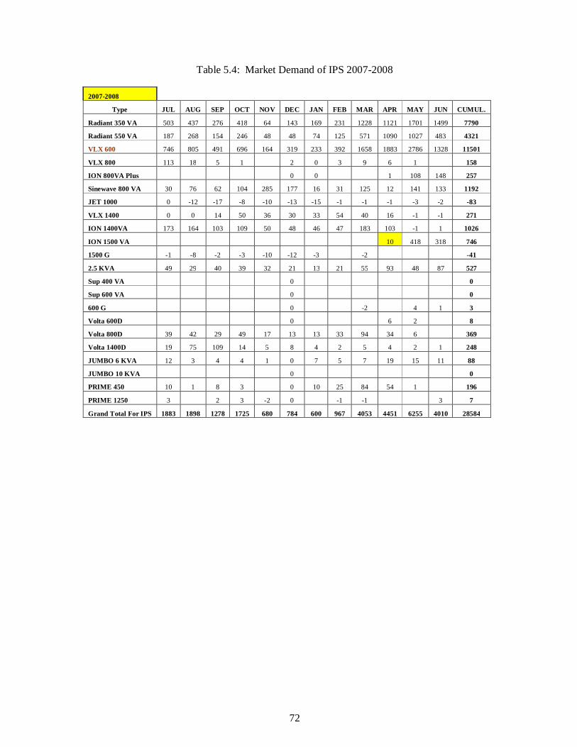
Table 5.4: Market Demand of IPS 2007-2008
2007-2008
Type JUL AUG SEP OCT NOV DEC JAN FEB MAR APR MAY JUN CUMUL.
Radiant 350 VA 503 437 276 418 64 143 169 231 1228 1121 1701 1499 7790
Radiant 550 VA 187 268 154 246 48 48 74 125 571 1090 1027 483 4321
VLX 600 746 805 491 696 164 319 233 392 1658 1883 2786 1328 11501
VLX 800 113 18 5 1 2 0 3 9 6 1 158
ION 800VA Plus 0 0 1 108 148 257
Sinewave 800 VA 30 76 62 104 285 177 16 31 125 12 141 133 1192
JET 1000 0 -12 -17 -8 -10 -13 -15 -1 -1 -1 -3 -2 -83
VLX 1400 0 0 14 50 36 30 33 54 40 16 -1 -1 271
ION 1400VA 173 164 103 109 50 48 46 47 183 103 -1 1 1026
ION 1500 VA 10 418 318 746
1500 G -1 -8 -2 -3 -10 -12 -3 -2 -41
2.5 KVA 49 29 40 39 32 21 13 21 55 93 48 87 527
Sup 400 VA 0 0
Sup 600 VA 0 0
600 G 0 -2 4 1 3
Volta 600D 0 6 2 8
Volta 800D 39 42 29 49 17 13 13 33 94 34 6 369
Volta 1400D 19 75 109 14 5 8 4 2 5 4 2 1 248
JUMBO 6 KVA 12 3 4 4 1 0 7 5 7 19 15 11 88
JUMBO 10 KVA 0 0
PRIME 450 10 1 8 3 0 10 25 84 54 1 196
PRIME 1250 3 2 3 -2 0 -1 -1 3 7
Grand Total For IPS 1883 1898 1278 1725 680 784 600 967 4053 4451 6255 4010 28584
72

Table 5.5: Market Demand of IPS 2008-2009
2008-2009
Item 08-Jul 08-Aug 08-Sep 08-Oct 08-Nov 08-Dec 09-Jan 09-Feb 09-Mar 09-Apr 09-May 09-Jun Total
IPS C/UNIT JUMBO-6KVA 1 1
IPS C/UNIT RADIANT -550 VA 1 4 2 2 13 13 35
IPS C/UNIT RADIANT -350 VA 5 3 1 1 23 1 34
IPS C/UNIT VOLTA -400 VA 384 121 46 55 125 285 56 2 5 1079
IPS C/UNIT IPS SUPREME-400 VA 1 1 15 2 19
IPS C/UNIT IPS SUPREME-600 VA 61 30 -10 81
IPS C/UNIT ION-1400 VA -5 -5
IPS C/UNIT ION - 2.50 KVA 1 -1 1 1
IPS C/UNIT POWER PLUS -750 VA 2 7 9
IPS CONTROL UNIT 800VA LB UPS 3 3
IPS CONTROL UNIT VOLTA 1400 D 1 3 -2 2
IPS CONTROL UNIT VOLTA 800 D 21 6 27
IPS CONTROL UNIT VOLTA 600 D -1 10 1 10
IPS C/UNIT ION SINEWABE 1500VA 2 1 3 2 7 2 3 4 7 1 8 40
IPS CON/UNIT DB SINEWABE 800VA 1 1 1 1 4
IPS C/UNIT COMPUVERTER VLX-600 2 1 1 2 2 2 10
IPS C/UNIT COMPUVERTER VLX-800 1 1
IPS C/UNIT COMPUVER VLX-1400VA 1 1
IPS C/UNIT PRIME - 450 VA 10 75 85
IPS C/UNIT PRIME - 1000 VA 7 3 6 16
IPS RADIANT 550VA - 400W 2HRS. 296 338 370 95 19 3 45 316 693 886 472 504 4037
IPS RADIANT 350VA - 280W 2HRS. 541 472 681 107 51 14 79 525 1273 1810 863 1020 7436
IPS ION 800 PLUS -640W 2HRS. 22 1 2 25
IPS COMP ION 1400VA-1120W 2HR. 1 1
IPS COMP ION 1500VA-1200W 2HR. 217 198 197 131 54 32 65 182 295 422 186 216 2195
IPS ION 2.50 KVA-2000W 2HRS. 50 47 52 30 18 10 9 9 28 28 11 14 306
IPS DB SINEWAVE 800-600W 2HRS. 136 199 226 68 33 39 54 171 309 448 130 204 2017
IPS VOLTA 800 D - 560W 2HRS. 1 1
IPS ION 3 KVA-2300W 2HR. 38 1 2 21 33 31 22 148
IPS VOLTA 400 VA -280W 2HRS. 56 116 95 41 11 -3 17 132 263 420 120 40 1308
IPS VOLTA 250 VA -160W 2HRS. 28 121 32 6 6 -1 11 34 90 128 22 21 498
IPS COMPUVE VLX 600-500W 2HRS. 788 1039 1016 334 131 48 266 833 1655 2902 730 1047 10789
IPS VLX 600-500W 2HRS. 98 98
IPS COMPUVE VLX 800-640W 2HRS. 5 5
IPS COM VLX 1400VA-1120W 2HRS. 2 2
IPS PRIME - 450VA 360W 2Hrs. 4 4
IPS PRIME - 1000 VA 800W 2Hrs. 8 6 4 18
IPS PRIME -1250VA 1000W 2Hrs. 4 8 1 1 3 2 1 20
IPS CONTROL UNIT 1000 JET-800W -2 -1 -2 -5
IPS JUMBO 6.0 KVA- 4500W 2HRS. 11 2 6 5 3 5 1 6 6 7 8 4 64
IPS JUMBO 10.0 KVA-7500W 2HRS. 6 3 4 1 1 3 3 5 12 4 3 45
Grand Total 2171 2934 2870 881 330 188 612 2344 4934 7337 2631 3233 30465
73

Table 5.6: Market Demand of IPS 2009-2010
2009-2010
Item 09-Jul 09-Aug 09-Sep 09-Oct 09-Nov 09-Dec 10-Jan 10-Feb 10-Mar 10-Apr 10-May 10-Jun Total
IPS C/UNIT RADIANT -550 VA 51 47 19 66 111 9 119 141 87 650
IPS C/UNIT RADIANT -350 VA 105 153 1 56 205 321 523 230 282 173 2049
IPS C/UNIT VOLTA -250 VA 15 4 2 21
IPS C/UNIT VOLTA -400 VA 2 89 3 94 IPS C/UNIT RADIANT-350 VA PLUS 0 IPS C/UNIT IPS SUPREME-400 VA 1 1 IPS C/UNIT IPS SUPREME-600 VA 1 1 1 1 1 2 7
IPS C/UNIT ION - 3 KVA 1 2 3 IPS CONTROL UNIT VOLTA 800 D 2 2 IPS C/UNIT ION SINEWABE 1500VA 4 3 8 1 1 5 6 25 11 20 84 IPS CON/UNIT DB SINEWABE 800VA 1 1 2 1 -1 1 5 IPS C/UNIT COMPUVERTER VLX-600 1 4 174 115 1 84 260 345 244 470 158 209 2065 IPS C/U COMPUVRTR VLX-600 PLUS 2 2
IPS C/UNIT PRIME - 1000 VA 2 5 1 1 9 IPS RADIANT 550VA - 400W 2HRS. 175 262 133 45 54 7 42 155 1390 1124 445 391 4223 IPS RADIANT 350VA - 280W 2HRS. 324 442 243 80 83 12 81 256 1162 889 475 418 4465 IPS RAD 350VA-280W PLUS 2HRS. 46 879 816 301 311 2353 IPS COMP ION 1400VA-1120W 2HR. 8 6 14 IPS COMP ION 1500VA-1200W 2HR. 132 197 114 61 51 23 57 113 448 462 243 211 2112
IPS ION 2.50 KVA-2000W 1 HR. 4 4
IPS ION 2.50 KVA-2000W 2HRS. 8 22 13 7 7 1 3 7 9 4 2 -1 82 IPS DB SINEWAVE 800-600W 2HRS. 102 174 80 43 81 19 26 88 581 465 233 215 2107
IPS ION 3 KVA-2300W 2HR. 24 35 30 20 31 28 15 24 71 82 52 48 460
IPS VOLTA 400 VA -280W 2HRS. 14 2 -1 1 47 66 1 130 IPS VOLTA 400VA-280W 2HRS PLUS 23 372 731 45 24 1195
IPS VOLTA 250 VA -160W 2HRS. 13 6 1 1 1 2 21 138 198 45 19 445 IPS COMPUVE VLX 600-500W 2HRS. 389 626 296 93 157 27 164 204 1035 865 454 354 4664
IPS VLX 600-500W PLUS 2HRS. 41 1214 1539 256 188 3238 IPS VLX 600-500W PREMIUM 2HRS. 60 130 175 365
IPS VLX 600-500W 2HRS. 149 215 109 58 60 15 35 145 374 251 135 99 1645 IPS JUMBO 6.0 KVA- 4500W 2HRS. 4 1 5 3 1 4 12 13 5 6 54 IPS JUMBO 10.0 KVA-7500W 2HRS. 7 1 4 3 1 3 4 9 5 1 38 IPS JUMBO10 KVA PLUS-7500W 2H. 2 6 2 1 11
Grand Total 1352 1996 1356 741 539 302 1007 2087 8476 8365 3420 2956 32597
74

Table 5.7: Market Demand of IPS 2010-2011
2010-2011
Item 10-Jul
10-Aug
10-Sep
10-Oct
10-Nov
10-Dec
11-Jan
11-Feb
11-Mar
11-Apr
11-May
11-Jun Total
IPS C/UNIT RADIANT -550 VA 149 449 51 100 23 49 94 242 418 202 89 134 2000
IPS C/UNIT RADIANT -350 VA 213 516 79 130 91 44 149 410 493 330 200 123 2778
IPS C/UNIT VOLTA -400 VA 2 2 IPS C/UNIT RADIANT-350 VA PLUS 0
IPS C/UNIT VOLTA -400 VA PLUS 1 1
IPS C/UNIT IPS SUPREME-400 VA 1 1
IPS C/UNIT IPS SUPREME-600 VA 6 3 1 1 1 1 2 1 16
IPS C/UNIT ION-1400 VA 1 1
IPS C/UNIT ION-800 PLUS 2 2
IPS C/UNIT ION - 2.50 KVA 1 1
IPS C/UNIT ION - 3 KVA 1 1 2 IPS CONTROL UNIT VOLTA 1400 D 1 1
IPS CONTROL UNIT VOLTA 800 D 1 1 IPS C/UNIT ION SINEWABE 1500VA 26 15 11 19 9 5 5 11 13 42 55 21 232 IPS CON/UNIT DB SINEWABE 800VA 1 83 25 13 53 59 92 76 59 34 495 IPS C/UNIT COMPUVERTER VLX-600 357 624 106 233 64 60 182 479 610 401 265 169 3550 IPS C/UNIT COMPUVERTER VLX-800 1 1 IPS C/UNIT COMPUVER VLX-1400VA 2 2
IPS RADIANT 550VA - 400W 2HRS. 591 553 200 270 37 22 71 269 736 445 275 469 3938
RAHIMAFROOZ 550VA IPS 5 10 3 2 3 1 7 31
IPS RADIANT 350VA - 280W 2HRS. 640 843 189 288 75 19 112 390 953 586 431 735 5261
IPS RAD 350VA-280W PLUS 2HRS. 316 468 62 164 46 14 39 147 635 366 43 14 2314 IPS COMP ION 1500VA-1200W 2HR. 241 247 140 195 67 70 94 112 244 155 196 288 2049 IPS DB SINEWAVE 800-600W 2HRS. 253 410 114 133 64 41 77 144 316 234 117 218 2121
IPS ION 3 KVA-2300W 2HR. 57 43 17 40 19 20 16 34 43 27 34 30 380
IPS VOLTA 400 VA -280W 2HRS. 1 1 IPS VOLTA 400VA-280W 2HRS PLUS 1 -1 1 1
IPS VOLTA 250 VA -160W 2HRS. 12 12 8 32 IPS COMPUVE VLX 600-500W 2HRS. 526 754 220 294 86 62 153 622 827 479 380 725 5128
IPS VLX 600-500W PLUS 2HRS. 218 286 30 94 26 22 29 121 148 82 49 56 1161 IPS VLX 600-500W PREMIUM 2HRS. 285 363 61 85 21 161 163 74 90 1303
IPS JUMBO 6.0 KVA- 4500W 2HRS. 5 4 2 7 5 3 1 2 3 7 5 9 53
IPS JUMBO 10.0 KVA-7500W 2HRS. 8 6 2 6 6 3 2 5 4 5 9 8 64
Grand Total 3901 5599 1301 2153 668 452 1081 3049 5696 3615 2283 3125 32923
75

Table 5.8: Market Demand of IPS 2011-2012
76
2011-2012
Item 11-Jul 11-Aug 11-Sep
11-
Oct 11-Nov
11-
Dec
12-
Jan
12-
Feb
12-
Mar 12-Apr 12-
May
12-
Jun Total
IPS C/UNIT RADIANT -550
VA 124 132 36 82 34 31 22 227 535 251 1474
IPS C/UNIT RADIANT -350
VA 101 182 64 103 34 41 37 362 379 559 1862
IPS C/UNIT IPS SUPREME-
600 VA 1 1 2
IPS C/UNIT ION - 3 KVA 2 1 3 11 1 18
IPS C/UNIT ION SINEWABE
1500VA 39 27 70 48 7 20 19 73 143 55 501
IPS CON/UNIT DB
SINEWABE 800VA 43 59 39 54 11 9 9 3 200 26 453
IPS C/UNIT COMPUVERTER
VLX-600 172 238 101 151 35 47 107 427 994 37 2309
IPS C/UNIT LUMINOUS-675
VA 296
IPS RADIANT 550VA - 400W
2HRS. 346 507 65 142 34 19 34 154 580 535 2416
RAHIMAFROOZ 550VA IPS 2 6 1 1 3 1 14
IPS RADIANT 350VA - 280W
2HRS. 417 530 101 165 15 21 26 133 1076 905 3389
IPS RAD 350VA-280W PLUS
2HRS. 69 88 43 70 2 3 12 56 23 366
IPS COMP ION 1500VA-
1200W 2HR. 211 131 71 100 20 23 32 106 305 242 1241
IPS DB SINEWAVE 800-600W
2HRS. 215 165 51 102 26 27 31 41 234 113 1005
IPS ION 3 KVA-2300W 2HR. 23 28 16 43 5 11 9 14 44 21 214
IPS COMPUVE VLX 600-
500W 2HRS. 653 469 130 219 41 28 57 204 1328 364 3493
IPS VLX 600-500W PLUS
2HRS. 30 33 8 10 1 1 22 12 117
IPS VLX 600-500W PREMIUM
2HRS. 50 58 17 24 2 1 6 21 179
IPS DIGIVERTER 600 VA-
440W 1.5 66 160 226
IPS VLX 600-500W 2HRS. 1 3 33 37
IPS JUMBO 6.0 KVA- 4500W
2HRS. 6 2 1 3 1 1 2 5 5 1 27
IPS JUMBO 10.0 KVA-7500W
2HRS. 10 3 5 2 2 2 1 25
Grand Total 2510 2654 819 1325 271 282 408 1853 5974 3568 0 0 19368
Related Documents