Demand and Supply

Demand and Supply

Headlines:

• On August 2, 1990, when Iraq invaded Kuwait, market price of crude petroleum jumped from $21.54 to $30.50 per barrel (almost 42% increase) before any physical reduction in the current amount of oil available for sale. One year later, the price of oil was $21.32 per barrel.

• In August 1987, a 386 PC sold at $6,995.In March 1992, the same computer sold at $1,495.Today Pentiums are cheaper then original 386 PCs.

Demand Curve• Amounts of a good purchased at alternative prices

• Inverse demand: maximum price paid for given quantity

• Law of Demand (ceteris paribus)

• Downward demand due to income and wealth effects• Downward inverse demand due to diminishing MU• Giffen's Paradox

Quantity

ID

Price

Price

D

Quantity

The Demand Function• An equation representing the demand curve

Qxd = f(Px , PY , I, N, A, Z)

Qxd = a0+a1Px+a2Py+a3I+a4N+a5A+a6Z

• Qxd = quantity demand of good X.

• Px = price of good X.

• PY = price of a substitute good Y.

• I = income.

• N = population

• A = advertisement

• Z = any other variable affecting demand (expectations, credit conditions)

Change in Quantity DemandedPrice

Quantity

D0

4 7

10

6

A

A to B: Increase in quantity demanded (due to change in the price of the good)

B

Price

Quantity

D0

D1

6

7

D0 to D1: Increase in Demand (due to change in demand determinants)

Change in Demand

13

Supply Curve• Amounts of a good produced at alternative prices.

• Inverse supply shows the minimum price required to produce given quantity of a good.

• Law of Supply (ceteris paribus)

• The supply curve is upward sloping

Quantity

Price

SPrice

Quantity

IS

The Supply Function• An equation representing the supply curve:

QxS = f(Px , PR ,PVI, PFI, Z)

Qxs = a0+a1Px+a2PR+a3PVI+a4PFI+a5Z

• QxS = quantity supplied of good X.

• Px = price of good X.

• PR = price of a related good (substitutes in production)

• PVI = price of variable inputs (labor, material, utilities)

• PFI = price of fixed inputs (land, buildings, machines)

• Z = other variable affecting supply (technology, government, number of firms, expectations)

Change in Quantity Supplied

Price

Quantity

S0

20

10

B

A

5 10

A to B: Increase in quantity supplied(due to change in the price of the good)

A

Price

Quantity

S0

S1

8

5 7

S0 to S1: Increase in supply (due to change in supply determinants)

Change in Supply

6

Mathematics of Equilibrium

Inverse Supply

Quantity supplied (Qs) and

Inverse Demand

P* = 133.33

Q* = 333.33 0

P = dQs - c = Qs - 200

P = a - bQd = 800 - 2Qd

a=800

Price (P)

c=-200

Slope is -b = -2

Slope is d = 1

Quantity demanded (Qd)

Marketequilibrium

Demand curve: Qd = 400 - ½P,Supply curve: Qs = 200 + P

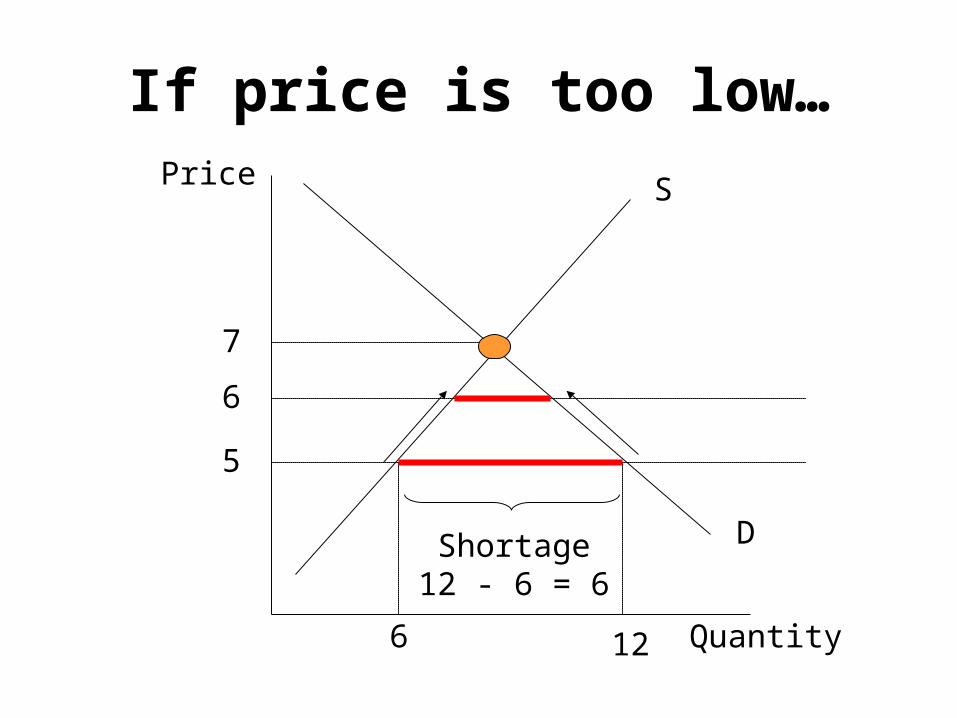
Price

Quantity

S

D

5

6 12

Shortage12 - 6 = 6

6

If price is too low…

7

Price

Quantity

S

D

9

14

Surplus14 - 6 = 8

6

8

8

If price is too high…

7

Consumer Surplus:The Continuous Case

Valueof 4 units

Price $

Quantity

D

10

8

6

4

2

1 2 3 4 5

Total Cost of 4 units

Consumer Surplus

Producer Surplus• The amount producers receive in excess of the amount

necessary to induce them to produce the good.

Price

Quantity

S0

Q*

P* Producer Surplus

Cost of Production

Comparative Statics: Effects of Changes in Demand and/or Supply

Increase in D increases both Q and P.

Increase in S increases Q and decreases P.

Increase in D and S increases Q and P = ?.

Decrease in D and increase in S decreases P and Q = ?.

Price Restrictions• Price Ceilings

• The maximum legal price that can be charged• Examples:

• Gasoline prices in the 1970s• Housing in New York City

• Price Floors

• The minimum legal price that can be charged.

• Examples:• Minimum wage• Agricultural price supports

Price

Quantity

S

D

P*

Q*

CeilingPrice

Qs

PF

Impact of a Price Ceiling

Shortage

Qd

Deadweight loss ofconsumer and

producer surplus

Opportunity Cost (Search &Black Market)

Full Economic Price• The dollar amount paid to a firm under a price ceiling, plus the

nonpecuniary price:

PF = PC + (PF - PC)

• PF = full economic price• PC = price ceiling• PF - PC = nonpecuniary price

• In 1970s ceiling price of gasoline = $1

• 3 hours in line to buy 15 gallons of gasoline

• Opportunity cost: $5/hr• Total value of time spent in line: 3 $5 = $15• Non-pecuniary price per gallon: $15/15 = $1

• Full economic price of a gallon of gasoline: $1 + $1 = $2

Impact of a Price FloorPrice

Quantity

S

D

P*

Q* QsQd

Surplus

PF

Cost of purchasingexcess supply

The Excise Tax

Quantity (thousands of CD players per week)

0 1 2 3 4 5 6 7 8 9 10

75

P1=100

130

DD

S

P2=105

P2-T=95

Tax Revenue

Consumersurplus

Producersurplus

S + tax

Deadweightloss

Price ($/CD player)

$10 taxBuyer pays (with tax)

Price beforetax

Seller receives(without tax)

P2 - P1 Buyer tax burden

P1 - (P2 - T) Seller tax burden

Excise Tax and the Demand

P2=P1+T=2.20

Thousands of insulin doses

P1 = 2.00

100

S

S + taxBuyer paysentire taxPPrice

Inelastic D

Thousands of pencils 1 4

P2-T=0.90

P1=P2=1.00S

Price Seller paysentire tax

Elastic D

S + tax

The more inelastic D, the more buyer pays: P2 = P1 + TBuyer burden: P2 - P1 =

(P1 + T) - P1 = TSeller burden: P1 - (P2 - T) =

P1 - (P1 + T - T) = 0

The more elastic D, the more seller pays: P2 = P1 Buyer burden: P2 - P1 =

P1 - P1 = 0Seller burden: P1 - (P2 - T) =

P1 - (P1 - T) = T

Excise Tax and the Supply

D

Bottles of spring water

P2-T=45

P1=P2=50

100

Inelastic S

Seller paysentire tax

Price

P2=P1+T=11

D

Thousands of pounds of sendfor computer chips

P1=10

3 5

Price

Elastic S

S + tax

Buyer paysentire tax

The more inelastic S, the more seller pays: P2 = P1

The more elastic S, the more buyer pays: P2 = P1 + T

The Ad Valorem Tax (% of Value)

Quantity (thousands of CD players per week)

0 1 2 3 4 5 6 7 8 9 10

75

P1=100

130

DD

S

P2=105

P2-T=95

Tax Revenue

Consumersurplus

Producersurplus

S(1 + tax)

Deadweightloss

Price ($/CD player)

$10 taxBuyer pays (with tax)

Price beforetax

Seller receives(without tax)

P2 - P1 Buyer tax burden

P1 - (P2 - T) Seller tax burden

MR

Demand and Revenue• Demand Function

Q = 70,000 – 100P

• Inverse Demand FunctionP = 700 – .01Q

• Total RevenueTR = P * Q = 700Q – .01Q2

• Average RevenueAR = TR / Q = 700 – .01Q = P

• Marginal RevenueMR = dTR / dQ = 700 – .02Q

For linear demand MR has the sameintercept and twice the slope of AR

• ARC Marginal RevenueArc MR = TR / Q

= (TR2-TR1) / (Q2-Q1)

-800

-600

-400

-200

0

200

400

600

800

0 10 20 30 40 50 60 70

P or AR

0

2

4

6

8

10

12

14

0 10 20 30 35 40 50 60 70