Deliverable 7.2: Overall Final Demonstration Report · IDE4L Deliverable 7.2 Overall Final Demonstration Report 8 ... The chapter describes the demo and lab sites – reported in

IDE4L is a project co-funded by the European Commission

Project no: 608860

Project acronym: IDE4L

Project title: IDEAL GRID FOR ALL

Deliverable 7.2:

Overall Final Demonstration Report

Due date of deliverable: 31.10.2016

Actual submission date: 31.10.2016

Start date of project: 01.09.2013 Duration: 38 months

Lead beneficial name: Unareti Spa, Italy

Revision [1.0]

Project co-funded by the European Commission within the Seventh Framework Programme (2013-2016)

Dissemination level

PU Public X

PP Restricted to other programme participants (including the Commission Services)

RE Restricted to a group specified by the consortium (including the Commission Services)

CO Confidential, only for members of the consortium (including the Commission Services)

IDE4L Deliverable 7.2 Overall Final Demonstration Report

2 IDE4L is a project co-funded by the European Commission

Track Changes

Version Date Description Revised Approved

v0r01 02/06/2016 Document template Della Giustina Davide (UNR)

v0r02 22/06/2016 L&P forecaster template Antimo Barbato (UNR)

v0r03 16/07/2016 State estimator template Antti Mutanen (TUT)

v0r04 18/07/2016 Power controller template Hannu Reponen (TUT)

v0r05 22/07/2016 FLISR template Amelia Alvarez (TUT)

V0r06 24/08/2016 Unareti State Estimator results

Antimo Barbato (UNR)

V0r07 30/08/2016 TUT Power controller results Anna Kulmala, Hannu Reponen (TUT)

V0r08 31/08/2016 RWTH, State Estimator and Power controller results

Andrea Angioni (RWTH)

V0r09 02/09/2016 TUT Power controller results Hannu Reponen (TUT)

V0r10 05/09/2016 LP Forecaster results presentation


V0r11 09/09/2016 State Estimator results Antti Mutanen, Ville Tuominen (TUT)

V0r12 12/09/2016 LP Forecaster and State Estimator contributions

Hormigo Maite (UFD)

V0r13 12/09/2016 FLISR review and results Alvarez Amelia (SCH) Dedè Alessio (UNR)

V0r14 13/09/2016 LV Power controller summarization

Hannu Reponen (TUT)

V0r15 13/09/2016 FLISR review and results Alvarez Amelia (SCH)

V0r16 14/09/2016 FLISR results and section integration

Alvarez Amelia (SCH)

V0r17 14/09/2016 PC results for Unareti demo site


V0r18 16/09/2016 SE results for OST demo site Mathias Christoffersen (DE)

V0r19 16/09/2016 SE and PC results review for RWTH lab site


V0r20 19/09/2016 SE results for OST demo site Mathias Christoffersen (DE)

V0r21 19/09/2016 SE results review Antimo Barbato (UNR)

V0r22 19/09/2016 LP Forecaster results review Hormigo Maite (UFD)

V0r23 20/09/2016 PC section review Hannu Reponen (TUT)

V0r24 20/09/2016 LP Forecaster review Mathias Christoffersen (DE)

V0r25 20/09/2016 Introduction, demonstrator description and use case mapping review


V0r26 26/09/2016 OST contributions review Mathias Christoffersen (DE)

V0r27 26/09/2016 FLISR TUT results integration Alvarez Amelia (SCH)



V0r28 26/09/2016 LV Power Control and MV sections review


V0r29 26/09/2016 State Estimator section review

Antti Mutanen (TUT)

V0r30 29/09/2016 MV section review Antti Mutanen (TUT), Andrea Angioni (RWTH)

V0r31 29/09/2016 FLISR section review Davide Della Giustina (UNR), Torben Vesth Hansen (OST), Alvarez Amelia (SCH)

V0r32 29/09/2016 PC section review Andrea Angioni (RWTH)

V0r32 29/09/2016 OST demo description and SE review

Mathias Christoffersen (DE)

V0r33 02/10/2016 FLISR section review, integration OST results

Torben Vesth Hansen (OST)

V0r34 02/10/2016 FLISR section review, integration OST results

Torben Vesth Hansen (OST)

V0r35 04/10/2016 FLISR section review and integration


V0r36 04/10/2016 State Estimator section review

Antti Mutanen (TUT)

V0r37 04/10/2016 FLISR section, Unareti demo description integration

Dedè Alessio (UNR)

V0r38 05/10/2016 State Estimator section, OST results review

Antti Mutanen (TUT), Mathias Christoffersen (DE)

V0r39 05/10/2016 PC section review Hannu Reponen (TUT)

V0r40 05/10/2016 Document review Davide Della Giustina (UNR)

V0r41 06/10/2016 Document review Antimo Barbato (UNR)

V0r42 06/10/2016 SE section review Antti Mutanen (TUT)

V0r43 11/10/2016 Document review Antimo Barbato (UNR)

V0r44 11/10/2016 MV section review Antimo Barbato (UNR), Andrea Angioni (RWTH)

V0r45 12/10/2016 SE section, UFD results review and chapter review

Antti Mutanen (TUT)

V0r46 17/10/2016 FLISR section review and integration


V0r47 17/10/2016 FLISR section, Unareti parts review

Dedè Alessio (UNR)

V0r48 26/10/2016 TUT BEO KPI value has been corrected

Álvarez Amelia (SCH)

V0r49 27/10/2016 Document review Mathias Christoffersen (DE)

V0r50 31/10/2016 Final review Stefano Zanini (UNR) Sami Repo (TUT)



TABLE OF CONTENTS

Track Changes ............................................................................................................................................................... 2

TABLE OF CONTENTS .................................................................................................................................................... 4

Executive Summary ...................................................................................................................................................... 6

1 Demonstrators descriptions ................................................................................................................................. 8

1.1 Oestkraft ....................................................................................................................................................... 9

1.2 Unareti ........................................................................................................................................................ 10

1.3 Unión Fenosa Distribución ......................................................................................................................... 11

1.4 TUT .............................................................................................................................................................. 12

1.5 RWTH .......................................................................................................................................................... 13

1.6 Schneider .................................................................................................................................................... 14

2 LV Load and Production Forecaster .................................................................................................................... 15

2.1 KPIs definition ............................................................................................................................................. 15

2.2 Demonstrations set-ups ............................................................................................................................. 15

2.3 Numerical Results and KPIs evaluation ...................................................................................................... 19

2.4 Conclusions ................................................................................................................................................. 28

3 LV Network State Estimator ............................................................................................................................... 29

3.1 KPIs definition ............................................................................................................................................. 29


3.3 Numerical results and KPIs evaluation ....................................................................................................... 31

3.4 Conclusions ................................................................................................................................................. 41

4 LV Power controller ............................................................................................................................................ 42

4.1 KPIs definition ............................................................................................................................................. 42


4.3 Numerical results and KPIs evaluation ....................................................................................................... 44

4.4 Conclusions ................................................................................................................................................. 53

5 MV Network State Estimator and Power Controller .......................................................................................... 54

5.1 MV Network State Estimator ...................................................................................................................... 56

5.1.1 KPIs definition ..................................................................................................................................... 56

5.1.2 Demonstration set-ups ....................................................................................................................... 56

5.1.3 Numerical results and KPIs evaluation ............................................................................................... 57

5.1.4 Conclusions ......................................................................................................................................... 61

5.2 MV Power Controller .................................................................................................................................. 62



5.2.1 KPIs definition ..................................................................................................................................... 62

5.2.2 Demonstration set-ups ....................................................................................................................... 62

5.2.3 Numerical results and KPIs evaluation ............................................................................................... 63

5.2.4 Conclusions ......................................................................................................................................... 67

6 FLISR.................................................................................................................................................................... 68

6.1 KPIs definition ............................................................................................................................................. 68

6.1.1 SAIDI KPI ............................................................................................................................................. 68

6.1.2 SAIFI KPI .............................................................................................................................................. 68

6.1.3 Breaker Energized Operations ............................................................................................................ 69


6.3 Numerical results and KPIs ......................................................................................................................... 75

6.3.1 Time Performances ............................................................................................................................. 76

6.3.2 FLIRS KPI .............................................................................................................................................. 87

6.4 Conclusions ................................................................................................................................................. 89

7 References .......................................................................................................................................................... 90



Executive Summary The objective of the deliverable D7.2 is to present and compare the results collected across field and lab sites, for

the verification and validation of the solutions proposed with the FP7 European project “IDE4L”. The deliverable

originates from the internal deliverable [D7.i] which was used for keeping track all the regular work done within the

WP7, documenting the effort, the work progress, the features that have been implemented, as well as the individual

and detailed results collected during the WP7 for each demo and lab site.

With respect to [D7.i], deliverable D7.2 is more focused on comparing the results among demo sites, in order to

draw the overall conclusions about the experimentations. Furthermore, the analysis is limited on the subset of use

cases highlighted in Figure 1, through a simplified version of the control hierarchy defined by IDE4L. The reason why

those components have been selected is that, together they model two very important business cases:

Congestion management business case, where:

- a portion of the network is monitored by collecting data from IEDs (monitoring use case),

- its status is determined through a state estimation algorithm (state estimation use case),

- pseudo-measurements are sent to the state estimator based on a forecast of load and

production profiles (load and production forecast use case),

- in case that forecast is missing, fixed profiles are used as a back-up input (not a use case),

- eventually, the network performance is optimized by the secondary (power) controller, issuing

set point to IEDs.

The Fault Location Isolation and Service Restoration, where IEDs are communicating based on a

peer-to-peer paradigm in order to solve clear faults on the network.

Figure 1: Simplified control hierarchy, with the emphasis on the components tested in field demonstrators.



The deliverable is organized as follows:

Chapter 1 presents a description of demo environments, both fields and labs sites.

Chapter 2 shows the results collected in testing the Load and Production Forecast (LPF) algorithm, designed

and developed with the WP5, in low voltage fields and lab sites.

Chapter 3 reports the results collected in testing the State Estimation (SE) algorithm, designed and

developed with the WP5, in low voltage fields and lab sites.

Chapter 4 presents the results collected in testing the Power Control (PC) algorithm, designed and

developed with the WP5, in low voltage fields and lab sites.

Chapter 5 reports the results collected in testing the Load and Production Forecast, State Estimation and

Power Control (PC) algorithm in medium voltage lab sites.

Chapter 6 presents the results collected in testing the Fault Location, Isolation and Service Restoration

(FLISR) system designed and developed within the WP4.



1 Demonstrators descriptions The chapter describes the demo and lab sites – reported in Figure 2 – that have been used to test the two business

cases within the project.

Figure 2. Lab and field demo sites.

For the sake of simplicity, Table 1 reports the mapping between the use cases tested in the project and the

demo\lab site where the test has been performed. The main features of each site are summarized in Table 2.

Table 1: Use cases vs. demonstrators mapping.

Use Case TUT RWTH TLV UFD OST UNR

MV Load and Production Forecast x

MV power control in Real Time operation x x

Decentralized FLISR x x x x

LV Load and Production Forecast x x x x x

LV State Estimation x x x x x

LV power control in Real Time operation x x x

Table 2: Main characteristics of demo and lab sites.

TUT RWTH UFD OST UNR

Use case type RTDS simulation RTDS simulation Real-life

demonstration

Real-life

demonstration

Real-life

demonstration

Network nominal

voltage

400 V

(line-to-line)

400 V

(line-to-line)

400 V

(line-to-line)

400 V

(line-to-line)

400 V

(line-to-line)

Network size 15 nodes 32 nodes 38 nodes 59 nodes 272 nodes

Number of

feeders

6 6 1 4 10



Number of load

nodes

13 32 7 54 228

Number of

production nodes

5 32 7 10 125

1.1 Oestkraft Oestkraft (OST) demo site (Figure 3) is located on the Northern part of Bornholm Island, in a residential area in the

village Tejn. It consists of two secondary 10/0.4 kV substations (namely no. 29 and no. 370) and a Low Voltage (LV)

network. The network consists of four LV lines with 126 customers. This area has been selected because of the

relatively high percentage of customers with heat pumps and PV panels.

In this area, 12 smart meters have been connected using a GPRS technology and transmit data every 15 minutes

with a resolution of 5 minutes. Additionally, the remaining 114 smart meters use a Power Line Communication (PLC)

technology and transmit data every 2 hours with a 5-minute resolution. The data from the meters are collected

once a day.

The Medium Voltage (MV) network is composed of one MV/MV (60/10 kV) substation, one MV line (No. 7) and 18

MV/LV (10/0.4) kV substations. Two MV/LV substations (namely no. 29 and no. 122) have been fully automated

with IED for monitoring, control, protection. To enable MV automation, an Ethernet/IP network has been

implemented by using optical fibres.

Figure 3: OST Demo Site. Tejn. Bornholm.



1.2 Unareti Unareti’s (UNR) field demonstrator is located in the city of Brescia in a district called “Il Violino”. This district was

recently established to promote an eco-compatible life-style (Figure 4): it is characterized by a high percentage of

customers equipped with PV panels, which is about 40 % of the total peak power demand, and using a district

heating system.

The LV field demonstrator consists of the whole LV network of a MV/LV substation, which has – in total – 10 LV

lines and feeds 294 customers, mainly residential ones. Out of all the nodes of the network, 45 (belonging to six out

of the ten LV lines) have been equipped with a new generation of smart meters, for a total of 60 meters that are

able to monitor in real-time a wide set of electric parameters of customers and PV units. Moreover, also six new PV

inverters have been installed for voltage and power regulations. For communication purposes, a Broadband Power

Line (BPL) over LV cables communication system has been used.

The MV network demonstrator consists of 1 MV/MV substation, 3 MV lines, 40 MV/LV substations and 9 MV

customers. Out of the three MV lines, two have been fully automated with monitoring, control, protection systems,

while the third one has been mainly involved in simulations and for the LV field trial. To enable the MV automation

services, a proper communication network has been implemented by using a mix of technologies, specifically

optical fibres, broadband power line over MV cables and Wi-Fi.

Figure 4: A picture from the UNR’s field demo.



1.3 Unión Fenosa Distribución Unión Fenosa Distribución (UFD) demo site is located in the headquarters of Antonio Lopez Street in Madrid (Figure

5). It consists of a LV network connected to a MV line fed by the primary substation ‘Puente Princesa’. The

substation is located on the southern edge of Manzanares River, close to the street, and it shares the facilities of

the University Corporate Company and offices of the high-voltage network operation.

UFD low voltage demo site has different facilities connected (already existing before the project) such as amorphous

photovoltaic installation (10 kW), monocrystalline photovoltaic installation (20 kW), polycrystalline photovoltaic

installation (20 kW), gas generator (5.5 kW), wind turbine (3.5 kW), two 3-phase EV chargers and a meteorological

station. Most of these installations have a smart meter connected, and all PV generators have controllable inverters.

Figure 5: UFD demo site location.



1.4 TUT The laboratory demonstration of TUT (Figure 6) consists of a Real-Time Digital Simulator (RTDS), commercial

Intelligent Electronic Devices (IEDs) and Substation Automation Units (SAUs). The main focus is the testing of

functional and non-functional performance of the MV and LV network monitoring and congestion management use

cases and automation system. Moreover, the laboratory tests are also used to extend the field demonstrations in

order to test additional scenarios and grid conditions (e.g. congestions due to over-dimensioning of the system)

and to consider additional resources (e.g. OLTC in secondary transformer).

Figure 6: TUT Lab Infrastructure.

Simulated LV network

Software

Hardware

Lab equipment

RTDS

RTU

(iRTU)

Database

DLMS

client

Load

forecast

(Python)

Adapter

MMS

client

Smart meters

(Landis&Gyr, Kamstrup)

AmplifierIsolation

transformer

Current

Voltage

MMS

server

Socket

TCP

AVR

(Unitrol)

Amplifier

Modbus to

IEC 61850

AVC

(REU615)

Production

forecast

(Python)

State

estimation

(Octave)

Real-time power

control (Octave)

To PSAU

SSAU

Set points to modelled

control devices and

measurements from

modelled measurement

devices

Set points to

real devicesMeasurements from real devices

PV

PV

PVPV

PV

PV

State

forecast

(Octave)

Analog IOGTAO GTNETx2 SKT

PB5

GTNETx2-SV

FLISR

(TLV)

FLISR

(TLV)

Amplifier Amplifier

IEC61850

GOOSE



1.5 RWTH The RWTH lab demonstrator for real time power system simulation is equipped with a real time digital simulator.

The installed RTDS is made up of 8 racks that can accurately and reliably simulate dynamics of power systems

generally in the range of 50 µs which can also be brought down to 2 µs in some special cases. In Figure 7, the RWTH

monitoring platform is represented.

The power system of Unareti is being modelled (both LV and MV) in four racks of RTDS. One rack for the LV grid

and three racks for the MV grid, respectively. The power profiles of passive and active users have been extracted

from past readings and given to the power system simulation in RTDS, in order to recreate realistic scenarios,

respectively for four intervals of 2 hours in working and weekend days of summer, autumn and winter seasons.

Furthermore, also some extra scenarios have been tested, respectively with instrument communication delay and

line congestions, in order to see the behaviour of the automation architecture in alternative stress cases. All these

scenarios have been used for testing state estimation and power control of MV and LV grids

The simulated Unareti power system has also been used to test the automation architecture defined in IDE4L. The

automation architecture consists of IEDs, both virtual and real, substation automation units and the communication

infrastructure. The virtual IEDs, the smart meters and the PMU provide the substation automation units at primary

and secondary substation with measurements.

Figure 7: RWTH monitoring platform.

SSAU virtual machine

Virtual IED in primary substations and MV

PSAU virtual machine

Virtual IED in secondary substations and LV

RTDS

MMS Client

MMS Server

WriteRead

MMS Client

MMS Server

Database

WriteRead

Database

Application:- State estimation- Power Control- Load forecast

MMS Client

MMS Server

Database

Application:- State estimation- Power Control- Load forecast

MMS Client

MMS ServerWriteRead

DNP3 Master

DNP3 Master

GTNET (DNP3 Slave)

Database

Digital connection

Digital connection

PMU

SM

GTAO

GPCs

Read

Read

C37.118 Client

DLMS/COSEM Client

Inte

rfac

e La

yer

Read

C37.118 Client

Inte

rfac

e La

yer



1.6 Schneider The laboratory deployed at Schneider (SCH) is set to test and demonstrate

the logic processing and distributed interaction as designed for IDE4L FLISR

solution based on IEC 61850 GOOSE messages exchange, the correct

selection of configuration parameters and the remote updating process

for the communication schemes and operation settings by means of an

IEC61850 MMS client.

The benefits of the lab deployment in Schneider is that it allows to test

and validate the logic implementation, the signal processing and the

communications between devices before the field deployment, thus

reducing the time that it will be needed in the field demo for installation,

start up and collecting data.

Within the IDE4L project, Schneider has developed a specific cabinet for

FLISR testing and validation (see Figure 8). This cabinet emulates a loop

distribution grid provided with a primary substation and four secondary

substations. Each substation is provided with a FLISR IED and two

controllable power interruption devices which position is monitored with

specific light devices. Power service provided to the lines controlled by

each secondary substation is also monitored by means of light indicators.

In order to emulate faults, the cabinet is equipped with push bottoms in

different positions of the grid that cause short-circuits increasing the

current sensed by the IEDs according to their location. IDE4L FLISR specific

solution considers the existence of two interruption technologies along

MV lines, deploying two steps IED interactions to control their operations.

Cabinet interruption devices could behave as reclosers or switches, thus

allowing the testing of different deployment configurations. All the IEDs

are connected through an Ethernet LAN using a network switch where

IEDs are able to exchange information regarding the fault event over

GOOSE protocol. A monitoring PC is also connected to the switch allowing

the logging and analysis of the GOOSE messages to determine correct

operation and response timing for different phases of FLISR operation. On

the service restoration phase, PC IEC 61850 simulation suites is used to generate MMS messages for FLISR

communication scheme and setting reconfiguration, testing the ability to adapt for the new grid topology.

Figure 8: Schneider Lab infrastructure.



2 LV Load and Production Forecaster Load and production forecasting provides an accurate prediction of the electric load and generation profiles in a

geographical area within a planning horizon. Within the IDE4L project, this algorithm works as a support tool to the

state estimation algorithm that is the core element in the congestion management of the low voltage network.

With the increase of intermittent power generation in the low-voltage and medium-voltage grids, the ability to

accurately forecast the relative load and production in the networks, several hours ahead, can indeed limit the

volatility of congestion management methodologies. The load and production forecast algorithm was

demonstrated in one laboratory (TUT) and in three electric utilities (UNR, UFD and OST).

2.1 KPIs definition In order to evaluate the performance of the load and production forecast algorithm, developed within the IDE4L

project, we use proper KPIs; here they are named Low Voltage Load and Generation Forecaster (LVLGF). These KPIs

are not completely consistent with the KPIs defined in the deliverable [D7.1]. These KPIs evaluate the deviation

between the forecasted values and the corresponding real measurements in terms of normalized root mean square

error. Specifically, its mathematical definition is reported below:

LVLGF (k) =100

𝑁∑

√1𝑇𝑛

∑ (𝑃(𝑡 + 𝑘)𝑛 − �̂�(𝑡 + 𝑘)𝑛,𝑡)2𝑇𝑛𝑡=1

max(𝑃𝑛) − min(𝑃𝑛)

𝑁

𝑛=1

where:

𝑘 : look-ahead time (e.g. 1-24 hours),

𝑇𝑛 : available time instants in the time period 𝑇 for node 𝑛,

𝑁 : number of nodes in the network,

𝑃(𝑡 + 𝑘)𝑛 : observed load/generation at node 𝑛 at time 𝑡 + 𝑘,

�̂�(𝑡 + 𝑘)𝑛,𝑡 : forecasted load/generation at node n for time 𝑡 + 𝑘, issued at time 𝑡,

min (𝑃𝑛), max(𝑃𝑛) : respectively, minimum and maximum measurement 𝑃 for node 𝑛 in the time period

𝑇.

2.2 Demonstrations set-ups Within the IDE4L project, the load and production forecast algorithm has been tested in several demo and lab sites.

In each of these sites, this algorithm has been used with a specific configuration as described in Table 3.

Table 3: LV load and production forecast algorithm configuration for each demo and lab site.

OST UNR UFD TUT

Use case type Real-life demonstration

Real-life demonstration

Real-life demonstration

RTDS simulation

Historical measurements type

Energy data [kWh] collected from smart meters

Energy data [kWh] collected from smart meters

Power data [kW] collected from smart meters

Power data [kW] aggregated from several customers

Historical measurements resolution

1 hour (aggregated from 5-minute measurements)

1 hour (aggregated from 15-minute measurements)

15 minutes 1 hour



Historical measurements availability

0 – 4 months depending on node

≥ 6 months per each meter

≈ 4 months per each meter

1 year per node + 1 year of verification data

Historical weather data

Temperature collected from forecast.io

Temperature and irradiation measurement data collected from the sensors installed at the substation premises

Temperature and irradiation collected by a meteorological station installed in the demo site

Temperature and irradiation

Historical weather data availability

> 3 years ≥ 1 year ≈ 4 months 1,5 years

Weather forecast data

24-hour temperature forecast

24-hour temperature and irradiation forecast profiles issued at 6:00 p.m., every day, by the local weather forecasts provider

24-hour temperature forecast

Historian data is used as forecast

Nodes for which forecast was produced

126 59 38 13

Type of loads for which forecast was produced

Majority are residential consumers, but also commercial buildings, street lighting and water supply loads are involved in the demonstration

Residential consumers

Office buildings Residential consumers

Type of generation source for which forecast was produced

- Photovoltaic panels

Photovoltaic panels

Photovoltaic panels

Test period 42 days 30 days 1 month 1 month

Execution mode Periodically, once every cycle time

Periodically, once every cycle time



Cycle time 24 hours 24 hours 1 hour 24 hours

Run time 00:00 00:00 Every hour 00:00

Forecast horizon 24 hours 24 hours 24 hours 24 hours

In order to clarify the several scenarios in which the load and production forecast algorithm has been tested, it is

also reported here, in reference to each demo and lab site, the input and output data of the algorithm for each

specific set up at customer premises, where:

𝑘 : current time

𝐸𝑡𝑜𝑡(𝑡) : net active energy at time t

𝐸𝑔𝑒𝑛(𝑡) : active energy generation at time t

𝐸𝑙𝑎𝑜𝑑(𝑡) : active energy load at time t



𝑃𝑔𝑒𝑛(𝑡) : power generation at time t

𝑃𝑙𝑎𝑜𝑑(𝑡) : power load at time t

𝑇(𝑡) : temperature at time t

𝑅(𝑡) : irradiance at time t

OST

In the OST demonstration, the smart meters are installed in such a way that they measure the combination of

electrical consumption and production, also when a local generation source is present. For this reason, the smart

meter only measures the overall power exchanged with the grid. In relation to the load and production forecasting,

this has resulted in only the load forecaster being executed and not the production forecaster. More details on the

different set-ups and on the input and output of the algorithm are reported in Figure 9.

Input:

- Historian Etot(t), T(t), t≤k

- Forecast T(t) t≥ k

Output:

-Etot(t) t> k

Input:

- Historian Etot(t), T(t), t≤k


Output:

-Etot(t) t> k

Smart Meter on the connection point

Case 1: customer with PV and one SM Case 2: customer without PV with the SM

Etot(k+1)

Etot(k+1)

Figure 9: LV load and production forecast algorithm set-ups in the OST demo site.

UNR

In the case of the UNR demonstration, several set-ups are found. The smart meters installed on the connection

points with the grid measure the overall demand and supply, while the PV meters only measure the net PV

production, as well as other PV-related measurements. Where local generation sources are present at customers’

premises and both the connection point smart meter and PV smart meter are installed, the algorithm provides both

load and generation forecasts. On the other hand, if one or both of these two meters are missing, the algorithm is

not able to provide any forecast because of missing input data. Where no local source is available at customers’

premises, the load forecasts are provided by the algorithm only if the smart meters are installed. More details on

the different set-ups and on the input and output of the algorithm are reported in Figure 10.



Case 5: customer without PV without the SM

Case 1: customer with PV and two SMs


Smart Meter on the PV

Case 3: customer with PV with only one SM o

Case 4: customer without PV with the SM

Input:

- Historian Eload(t), R(t), T(t), t≤k

- Forecast R(t), T(t) t≥ k

Output:

-Eload(t) t> k

Case 6: customer with PV, Shunt and two SMs

Case 2: customer with PV without any SM

Input:

- Historian Eload(t), Egen(t), R(t), T(t), t≤k


Output:

-Eload(t), Egen(t) t> kEload(k+1) Egen(k+1)

Not managed by the Load and Production Forecaster (Fixed Profiler is used in this case)

Eload(k+1) Egen(k+1)


Eload(k+1) Egen(k+1)

Eload(k+1)


Eload(k+1)

Input:



Output:


Figure 10: LV load and production forecast algorithm set-ups in the UNR demo site.

UFD

In the case of the UFD demonstration, there are two different set-ups. In the first one, a smart meter is used to

collect measurements related to customers and only the load forecasts are computed. In the second case, the smart

meter is installed to measure all the information related to local generation sources and only production forecasts

are provided by the algorithm. More details on the different set-ups and on the input and output of the algorithm

are reported in Figure 11.

Input:

- Historian Pload(t), T(t), t≤k


Output:

-Pload(t) t> k

Input:

- Historian Pgen(t), T(t), t≤k


Output:

-Pgen(t) t> k


Smart Meter on the generation source

Case 1: customer without PV with the SM Case 2: Generator (PV, GG, WT) with SM

Eload(k+1)Egen(k+1)

Figure 11: LV load and production forecast algorithm set-ups in the UFD demo site.

TUT

In the TUT lab site, we simulate the case in which local generation sources are installed at customers’ premises and

both the load and PV smart meters are present. More details on the different set-ups and on the input and output

of the algorithm are reported in Figure 12.



Case 1: customer with PV and two SMs


Smart Meter on the PV

Input:



Output:


Figure 12: LV load and production forecast algorithm set-up in the TUT lab site.

2.3 Numerical Results and KPIs evaluation

In order to evaluate the performance of the algorithm, the normalized root mean square error (NRMSE) defined as

explained in section 2.1 is analyzed. This KPI has been individually computed for load and generation forecasting,

as well as for each timeslot of the forecast horizon (i.e., 𝑘 in the KPI definition) to assess how the prediction accuracy

varies across the forecast horizon. Moreover, for statistical purposes, in addition to the overall KPI, this indicator

has been computed for each load and generation node of the network.

The NRMSE numerical results collected during the test campaign are presented in the following. Specifically, for

each timeslot of the forecast horizon, it is reported the NRMSE of the load and prediction forecasts, for each load

and production node of the network, as well as some additional metrics: median, 25th and 75th percentiles

(respectively lower and upper "hinges" in the figures), 1.5 of the Inter-Quartile Range (IQR) (i.e., the lower whisker

extends from the hinge to the lowest value within 1.5 * IQR of the hinge, the higher whisker extends from the hinge

to the higher value within 1.5 * IQR of the hinge).

OST

Results collected in the OST case are presented in Figure 13 in terms of NRMSE. In this case, no production forecast

was available for testing. Since the algorithm has been run once a day, starting from 0:00 a.m., the forecasting

horizon k also represent the real day hour (e.g., k=1 corresponds to 1:00 a.m.).



Figure 13: NRMSE of the LV load forecast algorithm as a function of the forecast horizon in the OST demo site.

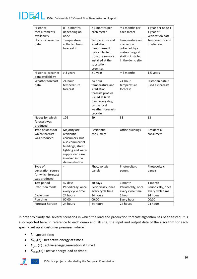
UNR

In the UNR case, both the NRMSE of the load and prediction forecasting are presented. Specifically, Figure 14

reports the results collected for the load prediction, discriminating them in terms of typology of consumers that

are classified based on their nominal (contractual) peak power (i.e. 3.3 kW or 4.95 kW). On the other hand, Figure

15 shows the numerical results found for each PV plant monitored through a smart meter, discriminating the results

in terms of typology of PV plants that are classified based on their nominal peak power (i.e. 1.29 kW, 4.11 kW and

5.6 kW). Notice that in case of 4.11 kW and 5.6 kW plants, no statistical metrics are presented since in the UNR

demonstrator only one PV plant was actually monitored for each of these two typologies. Moreover, no results are

reported for nightly hours in which the real production is zero and is trivial to be predicted. Since the algorithm has

been run once a day, at 0:00 a.m., the k value reported into the plot also represent the real day hour (e.g., k=1

corresponds to 1:00 a.m.).



Figure 14: NRMSE of the LV load forecast algorithm as a function of the forecast horizon in the UNR demo site.

Figure 15: NRMSE of the LV production forecast algorithm as a function of the forecast horizon in the UNR demo site.

UFD

In UFD case, both the NRMSE and RMSE of load and prediction forecasting are presented. Specifically, in Figure 16,

one reports the results collected for the load prediction, while in Figure 17 one shows the NRMSE for the prediction

forecast, where the considered generators are PV plants. There is no discrimination by contracted power, because

all consumers have the same peak power. Since the algorithm has been run once an hour, the k value is not

associated with any real day hour.



In the test campaign of the load and production forecaster, some issues were found in the UFD demo site,

specifically with reference to the monitoring system. In some cases, there were indeed interruptions in the data

gathering process, thus resulting in several gaps in collected data. As a consequence, the load and production

forecaster had a limited amount data to work with that explains the mediocre accuracy reported in Figure 16 and

in Figure 17.

Figure 16: NRMSE of the LV load forecast algorithm as a function of the forecast horizon in the UFD demo site.



Figure 17: NRMSE of the LV production forecast algorithm as a function of the forecast horizon in the UFD demo site.

TUT

In the TUT case, both the NRMSE of the load and prediction forecasting are presented. Specifically, Figure 18 reports

the statistical metrics of the KPI found for the load prediction algorithm, while Figure 19 focuses on the production

forecasting. Since the algorithm has been run once a day, at 0:00 a.m., the k value reported into the plots also

represent the real day hour (e.g., k=1 corresponds to 1:00 a.m.).

Notice that, in reference to the production prediction, TUT only had 1 PV panel measurements, which was

replicated to every node of the simulated network, having a generation source connected to. As a consequence, in

Figure 19 only the NRMSE is presented without any additional statistical metric since the test scenario consisted of

only one prediction node. Moreover, the NRMSE is available also at nigh hours since the simulations were run using

summer data and the sun does not completely set in Finland in that period of the year.



Figure 18: NRMSE of the LV load forecast algorithm as a function of the forecast horizon in the TUT lab site.

Figure 19: NRMSE of the LV production forecast algorithm as a function of the forecast horizon in the TUT lab site.

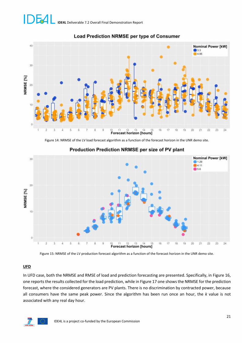
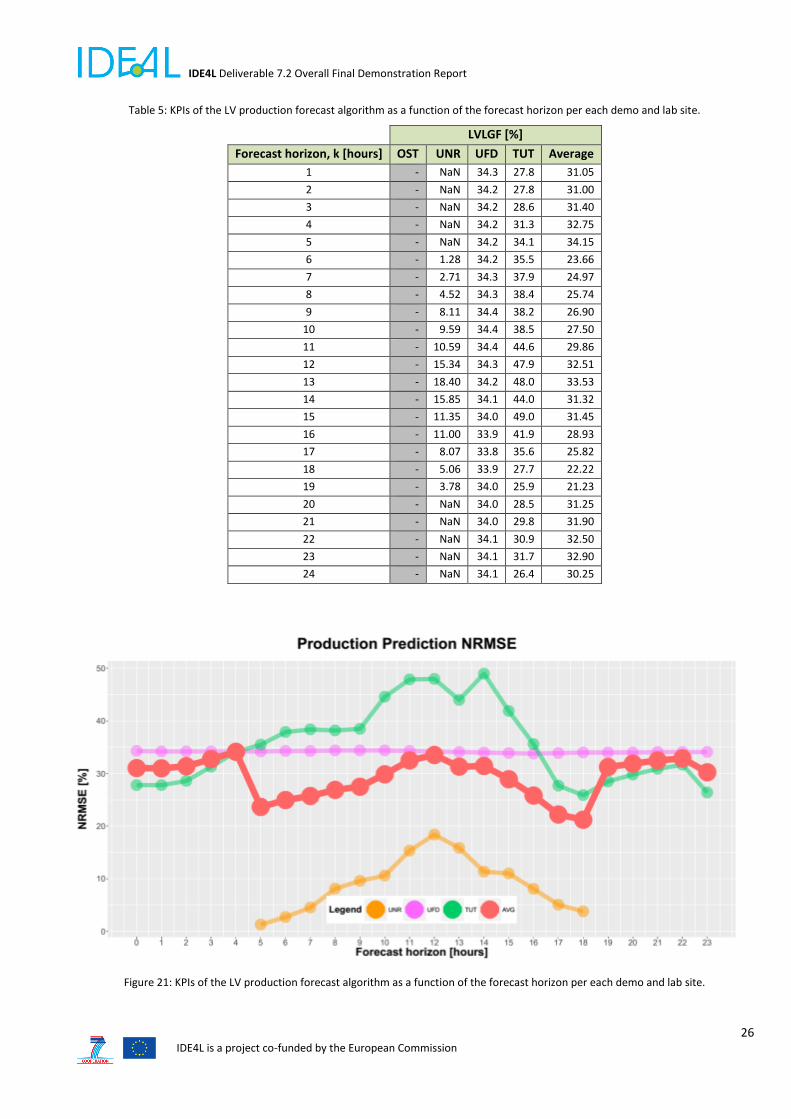
Comparison of use case results

In order to easily compare the results collected in demo and lab sites in reference to the load and generation

prediction, one reports in Table 4 and Figure 20 the KPIs obtained in the load forecast, while in Table 5 and Figure

21 one focuses on the generation prediction.



Table 4: KPIs of the LV load forecast algorithm as a function of the forecast horizon per each demo and lab site.

LVLGF [%]

Forecast horizon, k [hours] OST UNR UFD TUT Average

1 7.05 5.98 27.7 15.8 14.13

2 6.73 4.97 27.6 14.1 13.35

3 6.52 5.34 27.5 13.2 13.14

4 6.68 5.00 27.6 12.7 13.00

5 6.96 4.47 27.4 12.5 12.83

6 7.90 7.16 27.5 12.5 13.77

7 9.56 9.14 27.4 12.3 14.60

8 12.02 9.69 27.3 12.6 15.40

9 13.44 9.60 27.1 12.5 15.66

10 14.00 12.23 26.8 12.4 16.36

11 14.05 14.97 26.7 12.3 17.01

12 13.41 20.97 26.8 12.4 18.40

13 13.02 15.81 26.8 12.1 16.93

14 12.57 14.53 26.8 12.0 16.48

15 12.27 13.90 26.7 12.0 16.22

16 12.23 13.78 26.7 11.9 16.15

17 13.82 12.68 26.6 12.1 16.30

18 16.39 14.63 26.7 12.4 17.53

19 15.69 18.12 26.8 12.7 18.33

20 14.09 15.35 26.6 13.1 17.29

21 12.29 13.18 26.9 13.7 16.52

22 10.98 10.26 27.0 13.6 15.46

23 10.08 8.94 27.4 12.7 14.78

24 8.94 7.36 27.5 13.7 14.38

Figure 20: KPIs of the LV load forecast algorithm as a function of the forecast horizon per each demo and lab site.



Table 5: KPIs of the LV production forecast algorithm as a function of the forecast horizon per each demo and lab site.

LVLGF [%]

Forecast horizon, k [hours] OST UNR UFD TUT Average

1 - NaN 34.3 27.8 31.05

2 - NaN 34.2 27.8 31.00

3 - NaN 34.2 28.6 31.40

4 - NaN 34.2 31.3 32.75

5 - NaN 34.2 34.1 34.15

6 - 1.28 34.2 35.5 23.66

7 - 2.71 34.3 37.9 24.97

8 - 4.52 34.3 38.4 25.74

9 - 8.11 34.4 38.2 26.90

10 - 9.59 34.4 38.5 27.50

11 - 10.59 34.4 44.6 29.86

12 - 15.34 34.3 47.9 32.51

13 - 18.40 34.2 48.0 33.53

14 - 15.85 34.1 44.0 31.32

15 - 11.35 34.0 49.0 31.45

16 - 11.00 33.9 41.9 28.93

17 - 8.07 33.8 35.6 25.82

18 - 5.06 33.9 27.7 22.22

19 - 3.78 34.0 25.9 21.23

20 - NaN 34.0 28.5 31.25

21 - NaN 34.0 29.8 31.90

22 - NaN 34.1 30.9 32.50

23 - NaN 34.1 31.7 32.90

24 - NaN 34.1 26.4 30.25

Figure 21: KPIs of the LV production forecast algorithm as a function of the forecast horizon per each demo and lab site.



As can noticed from the results presented above, the load forecast algorithm assures an acceptable accuracy level

since the NRMSE overall average value is 15.58% and it varies from 4.47 % found in UNR case to 27.7% found in

UFD site. The inter-quartile range of the KPI is rather limited, with the 75th percentile typically lower than 20%. The

NRMSE has indeed values higher than its average value threshold only in a limited number of conditions and, as

one may notice from the UNR demo site-specific results presented in Figure 14, mainly in case of consumers with

greater hourly demands. In these cases, the variance of the energy demand of consumers is indeed greater, thus

resulting in less accurate predictions with greater medians and inter-quartile ranges.

The accuracy of the load forecast algorithm tends to be consistent when analyzed across the IDE4L demo sites, thus

confirming the applicability of the algorithm to real use-case scenarios. The only case in which KPIs have not been

satisfactorily met is represented by the UFD demo site, in which the performance of the algorithm has not been as

good as with the other sites. This result is due to limited data availability: as explained in reference to UFD-specific

results, in this demo site some problems were encountered with the monitoring system due to interruptions in the

data gathering process and gaps in collected data. As a consequence, the load and production forecaster had a

limited amount data to work with that explains the mediocre accuracy found in this case.

An interesting and intuitive conclusion that could be drawn out of the UNR and OST results is that the accuracy of

the load forecast algorithm is affected by the duration of the forecast horizon: the longer the forecast horizon, the

greater the NRMSE. Actually, this effect is caused by two other factors rather than by the length of the forecast

horizon: firstly, the NRMSE is a scale dependent indicator if analyzed across the forecast horizon since for each

customer\generation plant, all the hourly RMSE values are normalized by the same number (overall range of the

observed measurements in the observation period). As a consequence, greater values in the consumers’ demand

observed at given hours of the day imply greater values in the NRMSE. Secondly, the demand variance and volatility

are greater at day hours rather than at night hours, thus resulting in less accurate predictions with greater

normalized root mean square errors, greater medians and inter-quartile ranges. This independence between the

algorithm accuracy and the forecast horizon is particularly evident in the UFD demo site in which the NRMSE is

almost flat over the forecast horizon. This site is the only one in which the algorithm has been run every hour, thus

removing the dependency of the KPI on the specific hours of the day.

Similar considerations as those presented for the load forecast can be applied also to the production forecaster.

However, in this case, the accuracy found in predicting the generation profile is not as good as the one found in the

load forecasting: the NRMSE average value is 29.97 % and it varies from 1.28% found in UNR site, to 49% found in

TUT lab site. This result emphasize that generation profiles are more difficult to predict with respect to loads,

mainly because of the volatility of generation sources, as well as their dependency on the weather data forecast

accuracy.

The production forecast algorithm performance is strongly dependent on the size of the generation plant, as one

may notice from the UNR demo site-specific results shown in Figure 15. Specifically, the NRMSE tends to increase

as the nominal peak power of plants increases. In these cases, the variance of the energy generation profile is

indeed greater, thus resulting in less accurate predictions.

Unlike the load prediction, the production forecast accuracy tends to be not very consistent when analyzed across

the IDE4L demo and lab sites as one may notice by comparing the results shown above. This is probably due to

demonstration-specific conditions. Firstly, in the UFD case, some problems were encountered with the monitoring

system with interruptions in the data gathering process and gaps in collected data. As a consequence, as in the load

forecaster case, also the production forecaster had a limited amount data to work with that explains the mediocre



accuracy found in this demo site. As for TUT, results obtained are not very meaningful from a statistical point of

view since they have been obtained with only one PV panel.

2.4 Conclusions

The low voltage load and production forecast demonstrations were successfully finalized in the IDE4L experimental

campaigns, as well as in lab sites; proving that the proposed algorithm works even if its performance may differ

depending on the conditions of use. Specifically, the demonstration of LV network load and production forecast

provided different results in the prediction of loads and generations. On one hand, the load forecast turned out to

be quite accurate and consistent across demo sites. On the other hand, the generation forecast showed less

accurate and consistent solutions, due to the volatility of renewable generation plants and to their dependency on

weather forecast. The latter emphasizes the need for a more advanced and customized algorithm to predict the

production of these kinds of sources. Finally, demonstration results showed that for both loads and generations,

the algorithm is very consistent in predicting power\energy data over a one day-horizon since no major degradation

was found in increasing the forecast horizon.



3 LV Network State Estimator

State estimation is a key enabler for active network control (e.g. power control algorithm in IDE4L project), since

the state of the network must be known in order to efficiently control a network with distributed resources. The

IDE4L LV network state estimator [D5.1] uses network data, real-time measurements, load and production forecasts

and fixed load and production profiles as inputs and, based on this information, estimates what is the most likely

state of the network at a given moment. The estimated quantities are node voltage magnitudes and node power

injections (i.e. load and production) and current flows in all network nodes and lines. The state estimation algorithm

was demonstrated in two laboratories (TUT and RWTH) and in three electric utilities (UFD, OST and UNR).

3.1 KPIs definition The KPIs used to evaluate the state estimator performance, have been defined in [D7.1]. Both normalized (LVSE_2)

and un-normalized (LVSE_1) KPIs have been defined. Since all demonstration sites have the same nominal voltage,

the un-normalized KPI is used when evaluating and comparing the voltage estimation accuracy. The load and

generator sizes are different in different demonstration sites and, in order to facilitate the comparison between

demonstration sites, also the normalized KPIs are calculated for the estimated powers.

KPIs used to evaluate the state estimation performance:

𝐿𝑉𝑆𝐸_1 = √1

𝑁𝑇∑ ∑(�̃�(𝑡)𝑛 − 𝑥(𝑡)𝑛)2

𝑇

𝑡=1

𝑁

𝑛=1

𝐿𝑉𝑆𝐸_2 = √1

𝑁𝑇∑ ∑ (

�̃�(𝑡)𝑛 − 𝑥(𝑡)𝑛

|max(�̃�𝑛) − min(�̃�𝑛)|)

2𝑇

𝑡=1

𝑁

𝑛=1

where:

𝑁 : number of studied state variables,

𝑇 : number of time intervals under study,

�̃�𝑛 : real instantaneous values for the state variable n at time t=[1,T],

�̃�(𝑡)𝑛 : real instantaneous value for the state variable n at time t,

𝑥(𝑡)𝑛 : estimated value for the state variable n at time t,

min (�̃�𝑛), max(�̃�𝑛) : respectively, minimum and maximum real measurement for state variable 𝑛.

3.2 Demonstrations set-ups

The LV network state estimation algorithm was tested in five demonstration\lab sites, each with its own specific configuration, considering network topology, measurement setup, algorithm execution time and testing period as described in Table 6.



Table 6: Demonstration setups used in LV network state estimation KPI calculation.


Use case type RTDS simulation RTDS simulation Real-life

demonstration

Real-life

demonstration

Real-life

demonstration

Network nominal

voltage

400 V

(line-to-line)

400 V

(line-to-line)

400 V

(line-to-line)

400 V

(line-to-line)

400 V

(line-to-line)

Network size 15 nodes 32 nodes 38 nodes 59 nodes 272 nodes

Number of

feeders

6 6 1 4 10

Number of load

nodes

13 32 7 54 228

Number of

production nodes

5 32 7 10 125

Measurement

setup (used as

input in state

estimation)

Secondary

substation

voltage

measurement

Secondary

substation

power flow

measurements

(PQ)

2 smart meters

on load nodes

(PQ)

5 virtual smart

meters on

production

nodes (PQ)

Secondary

substation

voltage

measurement

Secondary

substation

power flow

measurement

(PQ)

32 virtual smart

meters on load

nodes (PQ)

32 virtual smart

meters on

production

nodes (PQ)

Secondary

substation

voltage

measurement

Secondary

substation

power flow

measurements

(PQ)

7 smart meters

on load nodes

(PQ)

7 smart meters

on production

nodes, 6x(P) &

1x(PQ)

Secondary

substation

voltage

measurement

Secondary

substation

power flow

measurements

(PQ)

Secondary

substation

voltage

measurement

10 feeder

power flow

measurements

(PQ)

61 smart

meters

measuring

either load,

production or

their sum (PQ)

Pseudo-

measurements

Static

load/production

values (PQ)

Pseudo-

measurements

were not used as

full observability

was always

available through

real time

measurements

Load &

production

forecast (P)

Load &

production

forecast (P)

Fixed

load/production

profiles (P) + load

& production

forecast (P)

Algorithm

execution

frequency

1 min 1 min 5 minutes 30 min 5 min

Test period 10 minute 2 hours 19 hours 15 days 30 days

Special

circumstances

Large stepwise

changes in PV

output were

simulated during

this test period

- Smart meter at

the EV charging

point gives

erroneous values,

replaced with

fixed profile

Some network

nodes contain

several

customers. These

are treated as one

aggregated load

-

(P) = Only active powers were measured/forecasted.



(PQ) = Both active and reactive powers were measured/forecasted.

The inevitable large variability in demonstration setups rendered the direct comparison of KPIs challenging.

However, the comparison can be very useful when evaluating whether or not the state estimation algorithm has

performed as planned or if there have been some demonstration site-specific problems.

3.3 Numerical results and KPIs evaluation

In this section, the performance of the state estimation algorithm has been analysed in laboratory and field

demonstrations. Each demonstrator section contains figures and analysis of the results. The numerical results are

collected into the comparison section.

TUT

The RTDS simulations in TUT focused on abnormal situations rarely encountered in real networks. Therefore, the

results are not directly comparable with other use cases. Also, in order to test the algorithm performance in several

different conditions, the simulation runs were kept very short. The length of the simulation was often only 10–15

minutes.

The simulation sequences included, for example, large stepwise or steadily ramping changes in PV output power or

missing measurements. In these situations, the state estimation accuracy is not as good as in normal network

operation conditions. However, the accuracy was adequate, taken into account the severity of the simulated

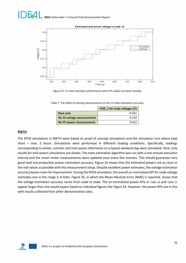
conditions. Figure 22 and Figure 23 show how the estimated voltage in node 12 compares with the real simulated

voltage in RTDS in two different test cases. Node 12 contains a PV power plant with 15 kW nominal power. In Figure

22, large stepwise changes (30 % of the nominal power) to PV output are caused and in Figure 23 the PV output is

increased in small steps from 37 % to 100 %. The node voltage estimation accuracy numbers, presented in the Table

7, are based on the simulation sequence shown in Figure 22. The base case includes all measurements mentioned

in the measurement setup part of the Table 6, and in the following cases either the substation voltage or PV power

measurements are assumed to be missing.

Figure 22: LV state estimator performance when PV output fluctuates.



Figure 23: LV state estimator performance when PV output increases steadily.

Table 7: The effect of missing measurements on the LV state estimation accuracy.

LVSE_1 for node voltages [V]

Base case 0.561

No SS voltage measurements 0.733

No PV power measurements 0.612

RWTH

The RTDS simulations in RWTH were based on proof of concept simulations and the simulation runs where kept

short – max. 2 hours. Simulations were performed in different loading conditions. Specifically, loadings

corresponding to winter, summer and mid-season afternoons on a typical weekend day were simulated. Here, only

results for mid-season simulations are shown. The state estimation algorithm was run with a one-minute execution

interval and the smart meter measurements were updated once every five minutes. This should guarantee very

good load and production power estimation accuracy. Figure 24 shows that the estimated powers are as close to

the real values as possible with this measurement setup. Despite excellent power estimates, the voltage estimation

accuracy leaves room for improvement. During the RTDS simulation, the overall un-normalized KPI for node voltage

estimates was in the range 2–4 Volts. Figure 25, in which the Mean Absolute Error (MAE) is reported, shows that

the voltage estimation accuracy varies from node to node. The un-normalized power KPIs in Table 10 and Table 11

appear larger than one would expect based on individual figures like Figure 24. However, the power KPIs are in line

with results collected from other demonstration sites.



Figure 24: “Phase A” active power for a generator in node FD3SC1A during mid-season loading condition in RWTH simulations.

Figure 25: Voltage estimation mean absolute errors for all customer nodes during one mid-season afternoon in RWTH simulations.

UFD



The UFD LV network was the smallest of real-life demonstration networks and the number of real time

measurements was high: every load and production node had a smart meter that sent the measured power values

to the database every 15 minutes, and therefore good estimation accuracy was expected in this demonstration.

The UFD demonstration was run for several weeks and several issues in the monitoring system were detected and

fixed. For example, the smart meter located at the electric vehicle charging point gave erroneous values and could

not be used as input in state estimation. Valid historical data from this metering point was also missing and

therefore the load & production forecaster could not supply pseudo-measurements for this node. These

measurements were replaced with a fixed EV charging profile. Sporadic interruptions in other measurements also

caused problems and in the end we had only a 19-hour time period when all the measurements had been working

simultaneously. This demonstration taught us the importance of backup pseudo-measurements. Fixed load profiles

for all load and production points would have reduced the state estimation errors during times when

measurements were missing and the load & production forecaster was unable to provide pseudo-measurements.

The following results are from a short time period between 6th of October 17.00 o’clock and 7th of October 12.00

o’clock.

The overall voltage estimation accuracy (LVSE_1) in this demonstration was 1.293 volts. Figure 26 shows that the

voltage estimation accuracy varies between 0.5 and 2.0 volts depending on the time of the day. Figure 27 and Figure

28 show that the voltage estimates for load and production nodes have similar accuracy.

The active power estimates for both load and production nodes were good, better than the pseudo-measurements

supplied by the load & production forecaster. This was mainly thanks to the numerous real time measurements

available in this demonstration. The KPI values for both estimated and forecaster active power are shown in Table

8.

Table 8: KPIs for LV load and production forecasts and estimates.

Load Production

LVSE_1 [W] LVSE_2 [-] LVSE_1 [W] LVSE_2 [-]

Forecasting accuracy 843 0.382 65.6 48.9

Estimation accuracy 646 0.185 0.037 0.028



Figure 26: Voltage estimation accuracy as a function of the time of the day (average accuracy on each hour) in UFD demo site.

Figure 27: Voltage estimation accuracy for load nodes (903–909) and production nodes (1104 & 1106) in UFD demo site.



Figure 28: Comparison of voltage estimation accuracy in different nodes and at different hours in terms of mean absolute error in UFD demo site.

OST

The demonstration in OST differs in measurement setup from all other demonstrations since in this case there were

no real-time smart meter measurements. The smart meter measurements were indeed read once a day. As a

consequence, the state estimator only relied on pseudo-measurements supplied by the load and production

forecaster. Moreover, in this demo there were no voltage measurements in load and production nodes and thus

the voltage estimation KPIs could not be calculated. Instead, the accuracy of load estimates was analysed.

The state estimation demonstration ran for two months, during which several issues in the demonstration system

configuration were fixed. Finally, the demonstration was completed, even if there were still a few issues in the

monitoring system. Specifically, the smart meter measurements stored into the database contained only imported

energy values and the exported energy values were not stored. Consequently, the PV production fed into the

network did not show in the smart meter measurements. However, the exported PV production showed in the

secondary substation measurements, and the state estimator was able to correct the loading level of the load nodes

to match the substation measurements. Figure 29 reports the total power flow on the secondary substation

according to secondary substation measurements, state estimates, smart meter measurements and load and

production forecasts. As one may notice, even though the forecasted load and production values were erroneous,

the state estimator was able to estimate the total load of the substation correctly. The state estimator compared

the measured secondary substation load with secondary substation load calculated with load and production

forecasts and if these were different, the difference was divided between measurements and forecasts in



proportion to their variances. Since the more accurate secondary substation measurements were given a higher

weight in this division, the majority of the difference between measured and forecasted substation load was

allocated to load and production nodes.

Because of the mentioned problem with monitoring system, the accuracy of final load estimates could not be

verified for all hours of the day, because the true daytime loads were unknown. Instead, KPI values for night-time

(20:00–08:00) were calculated. During this time, the customers with PV panels did not export any energy, and the

energy values collected by the smart meters were correct. The un-normalized KPI (LVSE_1) for estimated night-time

loads was 556 W and the normalized KPI (LVSE_2) was 0.235. Figure 30 shows the difference between night-time

and day-time estimation accuracy. Results from the demonstration are acceptable but large estimation errors were

observed in one network node that contained a large water supply unit. In order to find out what the state estimator

performance would have been without the measurement errors, a further investigation was conducted.

Specifically, off-line simulations using OST demonstration network and smart meter data were done to study what

the state estimator performance would have been without the above shown contradiction between secondary

substation and smart meter measurements. A few additional issues were discovered during the simulations. Load

forecasts for the fifth hour of the day were sometimes unavailable (which explains the significant RMSE spike in

Figure 30) and in the absence of load forecast accuracy information a bad assumption on the forecast accuracy had

been made. Once these issues had been corrected, the state estimator was able to improve the load forecasts.

Table 9 shows KPI values for one whole day and, as one may notice, the estimated loads were only marginally better

than the forecasted loads.

Figure 29: Total active power flow on the secondary substation according to secondary substation measurements, state estimator, smart meter measurements and load & production forecasts (30.8.2016) in OST demo site.



Figure 30: Average RMS error (LVSE_1) for active load estimates as a function of time of the day in OST demo site.

Table 9: KPIs for LV state estimation and load forecasting in OST demo site.

LVSE_1 [W] LVSE_2 [-]

Load forecasting accuracy 761 0.1646

Load estimation accuracy 741 0.1631

It is fair to conclude that considerable improvements in load estimation accuracy was not achievable with the used

real-time measurement setup, where real-time measurements are collected at the secondary substation and smart

meter measurements are collected once a day. The accuracy of the load estimation would benefit greatly if smart

meter measurements could be collected more often. Besides the mentioned issues, the state estimator performed

its duties flawlessly; it estimated node voltages, line current flows and secondary substation primary side power

flow. The estimates were stored into the database and could be used for power control and MV network state

estimation.

UNR

UNR had the largest demonstration network, over two hundred three-phase and single-phase network nodes. In

order to cope with the large network size, UNR had the best secondary substation measurements. Power flows

from the beginning of all LV feeders were measured, where as in other demonstration networks only substation

total power flows were available. The LV feeders were longer than in other demonstration networks and thereby

the voltage losses were larger and more difficult to estimate. The effect of this can be noticed in Figure 31 where

the un-normalized KPI for node voltage estimates is in the range 1.5–3.5 Volts. The voltage estimation accuracy was

low especially during day-time when network loading and voltage losses are high. Figure 31 shows also what would

have been the state estimation accuracy without the secondary substation measurements. Figure 32 shows that



nodes far away from the secondary substation have higher voltage estimation errors than nodes close to the

secondary substation.

During the studied time period, no problems in network monitoring, load and production forecasting or state

estimation algorithm itself were detected. However, there are some factors that might have affected to state

estimation accuracy and KPI calculation. The phase information of some loads, for example, was uncertain and the

voltage measurements available had only one-volt measurement resolution.

Figure 31: Voltage estimation accuracy in terms of RMSE per timeslot of the day with and without SS measurements in UNR demo site.



Figure 32: Voltage estimation accuracy as a function of the time of the day and electrical distance (impedance) from the secondary substation in UNR demo site.


The results from different demonstration sites were not always directly comparable. Nevertheless, such kind of

analysis was performed since a comparison of results could provide some insights on the state estimation

performance and feedback for improvements. Table 10 and Table 11 show the KPIs collected in the IDE4L

demonstrations, in terms of voltage and active power estimations.

In lab sites, collected results were not completely consistent in estimating nodes voltages. Specifically, in TUT RTDS

laboratory the algorithm showed a very good accuracy but the same kind of performance was not observed at the

RWTH RTDS laboratory even if in these two labs, the simulated networks were the same, although differently

reduced. At the moment, the reason for this difference is unknown. On the contrary, in reference to load estimate

KPIs, collected results turned out to be very similar between the two lab sites as one may notice from Table 11.

In real life demonstrations, UFD and UNR had good voltage estimation accuracy. Accuracy in UFD demonstration

was somewhat better. Both demonstrations benefitted from generous real-time measurements but the UFD

network was smaller and the voltage losses were lower, and this made voltage estimation easier. In OST

demonstration, the load estimates had smaller absolute errors than what was observed in laboratory

demonstrations or in UFD demonstration but relative errors were larger. In the OST site, smaller loads contributed

to lower absolute errors while higher relative errors were probably due to smaller amount of real-time

measurements.



Table 10: KPIs for LV voltage estimation.


LVSE_1 [V] 0.56 8.2 1.3 - 2.4

Table 11: KPIs for LV active power load estimation.


LVSE_1 [W] 866 808 646 556* -

LVSE_2 [-] 0.049 0.09 0.185 0.235* -

* Night time only

3.4 Conclusions

The demonstration of LV network state estimation proved to be more arduous than expected. Although the

demonstrations were carefully planned and designed, the differences in network structures, measurement setups

and data stored into the database caused several issues that had to be taken into account by making demonstration

case specific exceptions to the state estimation algorithm. This was often faster than fixing the issues in their root

cause but over time caused a mishmash of exceptions.

Problems in monitoring were frequent and since the state estimator relies heavily on input measurements and load

and production forecasts, which in turn rely heavily on the smart meter measurements, the state estimator

performance was often affected by issues in the monitoring systems. A reliable monitoring system plays a key role

in the state estimation performance. As learned from demonstrations, a bombproof backup solution for real-time

smart meter measurements and load and production forecasts should always be available to overcome potential

problems coming from missing measurements. In the IDE4L demonstration, such a backup solution was only

developed in the UNR demonstration. In UNR site, fixed load profiles were indeed available for all individual load

and generation points through an algorithm specifically designed and developed for this site within the IDE4L

project.

Despite several challenges, the LV network state estimation demonstrations were finalized and it was proven that

the developed state estimation algorithm works quite properly and provides an improved view to the state of the

network.



4 LV Power controller Real time power control (PC) is the key algorithm in secondary control designed and implemented in the IDE4L

project. The algorithm, whose details are described in [D5.2/3], is an optimization algorithm, that aims at

guaranteeing operations within acceptable network limits, while minimizing network losses and cost of control

actions such as tap changer operations or production curtailment. Reliable, correct and relatively fast operation of

the PC algorithm is vital to the distribution network congestion management. Within the IDE4L project, the

developed PC algorithm was demonstrated in TUT and RWTH RTDS laboratories, and field demonstrators were held

by UNR. UFD field demo site was used in successful beta-testing of the algorithm but the numerical results have

not been analyzed in details. In the field, the low-voltage power control (LVPC) was tested, and in the laboratory

environment both LVPC and medium-voltage power control (MVPC) were tested.

4.1 KPIs definition In deliverable [D7.1], 15 KPIs were defined to evaluate the operation of the PC algorithm. The KPIs were divided to

technical and economic, operational and technical safety parameters. In this deliverable, six main KPIs have been

selected to reflect the operation of the PC in case of different demonstrators. The selected KPIs are:

1. Curtailed production LVPC-E1: 𝑃𝑐𝑢𝑟 = ∑𝑖

𝑃𝑐𝑢𝑟, 𝑖

2. Network losses LVPC-E2: 𝑃𝑙𝑜𝑠𝑠 = 𝑃𝑡 + ∑𝑖

𝑃𝑝𝑟𝑜𝑑, 𝑖 − ∑𝑖

𝑃𝑙𝑜𝑎𝑑, 𝑖

3. Over-voltage volume LVPC-S1: ∑𝑖

∫ max (0, 𝑈𝑖 − 𝑈𝑚𝑎𝑥)

4. Under-voltage volume LVPC-S3: ∑𝑖

∫ max (0, 𝑈𝑚𝑖𝑛 − 𝑈𝑖)

5. Over-current volume LVPC-S2: ∑𝑖𝑗

∫ max (0, 𝐼𝑖𝑗 − 𝐼𝑚𝑎𝑥, 𝑖𝑗)

6. Average algorithm execution time LVPC-O_01.

Since the effectiveness and need for congestion management algorithms highly depends on the studied network,

it is not possible to directly compare the collected results among demonstrators as was the case with the load and

production forecaster and of the state estimator. Network losses, voltage profiles and feeders and transformer

loadings are strongly dependent on a variety of factors: network structure, component parameters, size, location

and temporary operation of loads and Distributed Generation (DG) units. As a consequence, the PC KPIs cannot be

scaled to be directly compared across demonstrators. Moreover, notice that the optimization and algorithm

outputs can be influenced by giving different values to the operational limits or cost parameters of the PC. Thus,

different outcomes in different laboratory and field scenarios were expected.

Even if KPIs cannot be scaled to be directly compared across demonstrators, the PC KPIs are meaningful when

evaluating the impact of the algorithm that is comparing the operation of individual networks with and without the

PC. The differences in the selected KPIs between the case with the PC and without it are calculated as follows:

2. Network losses: Δ𝑃𝑙𝑜𝑠𝑠 =𝑃𝑙𝑜𝑠𝑠_𝐵𝐿−𝑃𝑙𝑜𝑠𝑠_𝑃𝐶

𝑃𝑙𝑜𝑠𝑠_𝐵𝐿∙ 100%

3. Over-voltage volume: Δ𝑉𝑜𝑣𝑒𝑟 =𝑉𝑜𝑣𝑒𝑟_𝐵𝐿−𝑉𝑜𝑣𝑒𝑟_𝑃𝐶

𝑉𝑜𝑣𝑒𝑟_𝐵𝐿∙ 100%

4. Under-voltage volume: Δ𝑉𝑢𝑛𝑑𝑒𝑟 =𝑉𝑢𝑛𝑑𝑒𝑟_𝐵𝐿−𝑉𝑢𝑛𝑑𝑒𝑟_𝑃𝐶

𝑉𝑢𝑛𝑑𝑒𝑟_𝐵𝐿∙ 100%

5. Over-current volume: Δ𝐼𝑜𝑣𝑒𝑟 =𝐼𝑜𝑣𝑒𝑟_𝐵𝐿−𝐼𝑜𝑣𝑒𝑟_𝑃𝐶

𝐼𝑜𝑣𝑒𝑟_𝐵𝐿∙ 100%

The variables with the subscript BL are the baseline values of the particular KPI, i.e. the values without the PC. The

variables with the subscript PC are the KPI values with the PC. In laboratory demonstrations, these two sets of

values were calculated from two identical simulation sequences, run respectively with and without the PC



algorithm. In field demonstrations, this approach was obviously not possible and the baseline scenario could not

be determined at time the PC was run. As a consequence, in field demonstrators no comparison could be made to

evaluate the impact of the power controller.

4.2 Demonstrations set-ups For each LV Power control lab and field demonstration, the LVPC algorithm was configured according to Table 12.

Table 12: LV Power controller algorithm configuration.

TUT UNR RWTH

Use case type RTDS simulation Real-life demonstration

RTDS simulation

Network nominal voltage

400 V (line-to-line)



Voltage limits +/- 5 % +/- 5 % +/- 5 %

Cost function considers

1. Network losses and generation curtailment 2. Network losses, generation curtailment, number of tap changer operations and the voltage variation from a reference value

Network losses 1. Network losses and generation curtailment 2. Network losses, generation curtailment, number of tap changer operations and the voltage variation from a reference value

Network size 15 (three-phase) nodes

272 nodes 32 nodes

Number of feeders

6 10 6

Number of load nodes

13 228 32

Number of production nodes

5 125 32

Controllable resources

Transformer tap-changer Active/Reactive power of 5 DG units

PV inverters of 6 PV panels

Load/Production active and reactive power set points. OLTC at secondary substation.

Algorithm execution frequency

1 min 5 minutes 10 min

Test period 4-30 minutes in one sequence

15 days 80 - 125 minutes

Scenarios:

Multiple sequences using DG real powers and supply network voltage changes as disturbances

- Winter, Summer, Mid-Season typical weekend day scenarios.



4.3 Numerical results and KPIs evaluation In this section, the performance of the PC algorithm has been analysed in laboratory and field scenarios. Each

demonstrator section provides further details of the scenario where the PC algorithm has been used. Figures of

network voltages, and available and utilized resources are provided to give further insights, in addition to the KPIs,

on the effect of the low voltage power controller in each studied network. Finally, the improvement the network

performance due to PC is analysed in Table 16 - Table 19 .

TUT

To demonstrate the functionality and performance of LVPC, in TUT laboratory two scenarios and multiple test

sequences were created. Network generation and loading conditions were derived according to DSO’s data. The

simulation sequences were planned such that they would test the PC algorithm as thoroughly as possible. The

sequences used are not likely to occur in real distribution networks, but the changes in loading and production are

usually slower. Changes in DG real powers and supply network voltage were used as disturbances in the simulation

sequences and simulations were conducted with different cost parameters of the PC algorithm cost function. In this

deliverable, only one TUT simulation sequence is presented. More detailed information regarding other sequences

simulated in TUT can be found in [Reponen ISGT] and [Reponen MSc].

In the example simulation sequence, the nominal powers of the real DG units have been multiplied by three, which,

as desired, leads to over-voltages in some loading and generation situations. The duration of the sequence is 30

minutes and the sequence goes through the maximum and minimum loading conditions with different production

situations. The changes in DG output powers and loadings in the sequence are presented in Table 13. The same

sequence was run both without and with the PC. The acceptable voltage range was set to ±5 % in PC algorithm

configuration.

Table 13: TUT LV power control simulation sequence.

Time DG output factor Loading conditions

0 s 3.0 MIN

170 s 0.9 MIN

710 s 0.9 MAX

1250 s 3.0 MAX

Network voltages in the baseline simulation are presented in Figure 33. The results show that some node voltages

are outside the acceptable voltage range regardless of the network loading conditions when the DG units are

producing at three times the nominal value. This kind of operation is not acceptable.



Figure 33: LV Network voltages in baseline simulation in TUT site.

Network voltages obtained when using the PC with the same simulated sequence are presented in Figure 34. Also

in this case, a momentary overvoltage can be seen. This is due to substantial change to the outputs of the DG units

in the sequence as seen from Figure 35. However, after the PC algorithm has completed its control actions, the

voltages are restored back between the acceptable voltage limits. Tap changer operations have the greatest effect

on voltages in LV networks, which can be triggered by changing the Automatic Voltage Control (AVC) relay

substation voltage reference as seen in Figure 37.

Figure 34: Network voltages with the LVPC algorithm operating in TUT site.



Figure 35: Real power generation of DGs in the scenario in TUT site.

Figure 36: Reactive power generation of DGs with LVPC in TUT site.



Figure 37 Measured and estimated secondary substation voltages, and AVC relay voltage set point in LVPC scenario in TUT site.

KPI values calculated in the two simulation cases are presented in Table 14. The KPI calculation shows that the

overvoltage volume is lower in the PC case. Also the duration of over-voltages is significantly lower as can be seen

from Figure 33 and Figure 34. On the other hand, the losses are in this case higher with the PC due to two reasons.

Firstly, the PC utilizes reactive power control according to Figure 36 to decrease the voltage level that increases the

losses compared to the baseline case where unity power factor is used for the DG units. Moreover, the voltage level

is in the baseline case higher when the DG units are producing their maximum output and, therefore, the losses are

smaller since the loads in the network are modelled as constant power loads.

Table 14: KPI values in TUT baseline and PC simulation cases.

Baseline Low Voltage Power Control

Curtailed production not applicable 0

Network losses [kWs] 8252.3 8357.7

Over-voltage volume [pu * s] 3.30 2.68

Under-voltage volume [pu * s] 0.0 0.0

Over-current volume [A*s] 0.0 0.0

Average algorithm execution time [s] not applicable 13.99

It should be noted that in the considered baseline case the network operation is not acceptable. Network

reinforcement would be obligatory if the simulated artificial amount of DG would be connected to the considered

network.

UNR

In the UNR case, it is here presented an extract of the PC algorithm operation during the 15-day test-period. Figure

38 presents network voltages on a given test day, while Figure 39 shows the minimum and maximum voltage values

during the same time period. It can be noticed, on this day, as well in the remaining testing campaign of the PC

algorithm, no voltage violations outside acceptable voltage range have been observed due to the current

penetration of PV generation in the network. As a consequence, during the demonstration the available

controllable resources in the network, that are 6 PV inverters, have been utilized with the goal of reducing reactive



power flows, and thus network losses. Figure 40 reports an example of the reactive power profiles of controlled

resources during the testing campaign of the PC algorithm.

Figure 38: RMS voltage for 30 nodes on September 10, 2016 in UNR demo site.

Figure 39: Minimum and maximum RMS voltage profiles on September 10, 2016 in UNR demo site.



Figure 40: Reactive Power profiles for LV nodes on September 10, 2016 in UNR demo site.

Utilization of small-scale of reactive power has minor effect on network voltages due to the reactance/resistance

ratio of lines in LV networks. In the UNR case, the cost function was set to minimize network losses, where the

effect of reactive power flows can be seen. This demonstration confirms that the LVPC application has been

successfully installed, and set points of available controllable resources have been successfully altered, in real LV

distribution network operations.

RWTH

In the RWTH case, three scenarios have been exploited to test the low voltage power control use case. These

scenarios consist of a typical afternoon scenario of winter, summer and mid-season weekend. The simulations, each

of 1-2 hours, were connected in real time with the IDE4L automation platform consisting in the set of IEDs and SAUs

that send power control set points.

In Figure 41, the voltage RMS of the node voltages over the simulation time are presented. The time and date refer

to the time during which the simulation was run and not the “simulated” time of the year. In Figure 42 and Figure

43, active and reactive power profiles of resources are shown. Finally, the OLTC commands and status are shown

in Figure 44. The figures refer to the summer weekend afternoon scenario. As one may notice, the voltage maintains

proper status in the nodes, between the voltage bounds, during the simulation time. Similar conclusions are also

valid for the current limits of the lines. In such conditions, the optimization function is mainly used to reduce

network losses.



Figure 41 RMS voltage time profiles for LV nodes for Midseason weekend day afternoon in RWTH lab site.

Figure 42 Active Power time profiles for LV nodes during Midseason weekend afternoon scenario in RWTH lab site.



Figure 43 Reactive Power time profiles for LV nodes during Midseason weekend afternoon scenario in RWTH lab site.

Figure 44 OLTC tap position during Midseason weekend afternoon scenario in RWTH lab site.

The numerical results of the three scenarios are presented in Table 15.



Table 15: KPI values in RWTH simulation scenarios for LVPC algorithm.

Summer weekend day

afternoon

Winter weekend day

afternoon

Mid-Season weekend day

afternoon

Total duration [min] 135 120 80

Curtailed production [kWh] 0 0 0

Network losses [kWs] 20753 19161 6065

Number of Alerts 5 0 0

Under-voltage volume [pu * s] 2.13 0 0

Average algorithm execution

time [s] 400 255 205


As mentioned earlier, the PC KPIs cannot be scaled so to directly compare the PC operation in different

demonstrators or scenarios. However, the impact of the PC on the KPIs can be analysed and compared when the

baseline scenario is available as is in lab sites. Table 16 - Table 19 list the KPIs computed in the IDE4L test campaign.

Positive value in the table indicates improvement in such KPI when comparing case with PC to the baseline scenario.

The average algorithm execution time in Table 20 gives insights on how the network size, and type and amount of

controllable resources affect the algorithm execution time. The mid-season weekend day afternoon scenario was

used in calculation for the RWTH values.

Table 16: Network losses KPI change for LVPC.

TUT RWTH

Network losses [%] -1.2 7.9

Table 17: Over-voltage volume KPI change for LVPC.

TUT RWTH UNR

Over-voltage volume [%] 18.8. 0 0

Table 18: Under-voltage volume KPI change for LVPC.

TUT RWTH UNR

Under-voltage volume [%] 0 0 0

Table 19: Over-current volume KPI change for LVPC.

TUT RWTH UNR

Over-current volume [%] 0 0 0

Table 20: Average algorithm execution time for LVPC.

TUT UNR RWTH

Average algorithm execution time [s] 13.99 68.6 205



The short simulation in TUT scenario with PC eventually led to great improvement in over-voltage volume, but

resulted in increased network losses. However, such network operation in the baseline scenario is not permissible

from the DSO’s point of view. In normal permissible operation, the longer RWTH simulation scenario demonstrated

the reduction in network losses using PC. From field the baseline losses were unavailable and the improvement

could not be calculated. The other technical safety parameters did not differ across the demonstrators and network

was operated within permissible under-voltage and over-current limits.

The comparison further confirms that with the free Octave SQP solver used in the project, the performance of the

optimization is heavily dependent on network size, and the type and amount of controllable resources in the

network. With the lowest number of network nodes, lowest algorithm execution times were achieved. Due to this

fact, the acceptable algorithm execution frequency had to be increased accordingly for each demonstrator. In order

to obtain better performance in this manner, a commercial solver to the optimization problem should be used.

4.4 Conclusions The results presented in this deliverable confirm that the proposed and implemented PC algorithm operates in all

the demonstration cases as expected and that no adverse time domain operation occurs. Also, the results show

that the algorithm is able to improve the defined KPIs in all the demo cases. The benefit of the PC algorithm varies

by network and each individual case should be evaluated using the planning principles presented in [D3.3]. In

general terms, it can be said that the weaker the network and the larger the amount of generation connected to it,

the larger the benefits of the PC.

It should be noted that the KPIs presented above are calculated based on a relatively short period of time and are,

therefore, only suggestive. To be able to properly evaluate the effectiveness of the PC in a particular network, yearly

calculations have to be conducted [Kulmala IET GTD]. Some yearly calculations for the UNR demo network have

been conducted in [D3.3] which show that on a yearly basis the proposed PC algorithm is able to both prevent

voltage and current congestions and to decrease the annual network losses.



5 MV Network State Estimator and Power Controller

The medium voltage portion of the grid is included in the IDE4L demonstrations through real time laboratory

demonstrations. The portion of grid tested is composed of three feeders of Unareti distribution network. The model

is imported into RTDS software and hardware environment as depicted in the model reported in Figure 45. The MV

part and the LV part are simulated in the same environment, as well as their automation systems. In fact, the

Medium Voltage State Estimator (MVSE) and low voltage state estimator exchange the estimation results at the

secondary substation in real time. Similarly, the Medium Voltage Power Controller (MVPC) and the low voltage

power controller are shifted in time, in order not to create any control action conflict. In the next sections, the

results of MV state estimation and MV power control demonstrations are presented.



Rack 2

Rack 1

Rack 3

Rack 4

Figure 45: Feeder 1,2,3 and LV grid simulated on RTDS rack 1,2,3 and 4.



5.1 MV Network State Estimator The MV network state estimator is used to estimate voltages, loads, production, and current flows in all network

nodes and lines.

5.1.1 KPIs definition

In order to evaluate the state estimator accuracy in estimating nodes voltage, the following KPI is used, as also

described in [D7.1]:

𝑀𝑉𝑆𝐸_1 = √1

𝑁𝑇∑ ∑(�̃�(𝑡)𝑛 − 𝑥(𝑡)𝑛)2

𝑇

𝑡=1

𝑁

𝑛=1

where:

𝑁 : number of studied state variables,

𝑇 : number of time intervals under study,

�̃�(𝑡)𝑛 : real instantaneous value for the state variable n at time t,

𝑥(𝑡)𝑛 : estimated value for the state variable n at time t.

5.1.2 Demonstration set-ups

The MV network state estimation algorithm has been demonstrated in one lab site, namely RWTH, whose specific

configuration in terms of network topology, measurement setup, algorithm execution time and testing period is

described in Table 21.

Table 21: MV network state estimator simulation setup.

RWTH

Use case type RTDS simulation

Network nominal

voltage

15000 V

(line-to-line)

Network size 40 nodes

Number of

feeders

3

Number of load

nodes

39 (+1 from the aggregated LV grid)

Number of

production nodes

39 (+1 from the aggregated LV grid)

Measurement

setup (used in

state estimation)

Substation voltage magnitude and power flow

Power active and reactive injection at the load and generators.

Pseudo-

measurements

Load/Production from forecast. Not used as the observability was always

available through real time measurements.



Algorithm

execution

frequency

1 min

Test period 2 hours

5.1.3 Numerical results and KPIs evaluation

State estimation tests have been conducted in three scenarios: winter, summer and mid-season afternoons of a

typical weekend day. The testing scenarios lasted for 2 hours each. State estimation is performed by the SAU on

regular intervals of 1 minute. The devices at each MV node provide active and reactive power injections, as well as

voltage magnitudes. The algorithm, however, only reads voltage magnitude for the substation and power injections

related to prosumers’ nodes in order to test the algorithm in conditions that are not overly favourable. Given that

power injection is available in all nodes, the condition of observability is satisfied without the need of using pseudo-

measurements.

Figure 46, Figure 47, Figure 48, Figure 49 and Figure 50 show a comparison between measured and estimated

electrical quantities, respectively in terms of voltage magnitude, absorbed active and reactive power and generated

active and reactive power for phase A of bus 0545 of the MV grid in the mid-season weekend afternoon scenario.

Bus 0545 is the first load node in MV feeder 2. The voltage offset is due to the simulation blocks used in RTDS to

connect subsystems in simulation that are not easy to compensate. Notice that the x-axis of plots represent the

real time during which the simulation was running (totally two hours). The relative error due to such components

is anyhow very low. Power injection estimation is also accurate.

Figure 46: Comparison between voltage magnitude measurement and estimation for phase A of bus 0545 of MV grid in the Mid-season

afternoon weekend scenario.



Figure 47: Comparison between absorbed active power measurement and estimation for phase A of bus 0545 of MV grid in the Mid-season

afternoon weekend scenario.

Figure 48: Comparison between absorbed reactive power measurement and estimation for phase A of bus 0545 of MV grid in the Mid-

season afternoon weekend scenario.



Figure 49: Comparison between generated active power measurement and estimation for phase A of bus 0545 of MV grid in the Mid-


Figure 50: Comparison between generated reactive power measurement and estimation for phase A of bus 0545 of MV grid in the Mid-


Table 22-Table 26 present the KPIs obtained for the performance of state estimation in MV network. As a general

conclusion, we can observe that the injection of power and current as well as voltage are properly estimated. Based

also on what is reported in the figures, one can assume that a portion of error is due to the rate of estimation (1

minute) which is slower than the update rate of the measurements. With higher update rate, the estimation may

indeed better follow the changes in power and voltage.



Table 22: KPIs for MV voltage estimation.

RWTH

MVSE_1

[V] 43.75

Table 23: KPIs for MV active power load estimation.

RWTH

MVSE_1 [W] 1760

MVSE_2 [-] 0.14

Table 24: KPIs for MV reactive power load estimation.

RWTH

MVSE_1 [VAr] 246

MVSE_2 [-] 0.14

Table 25: KPIs for MV active power generation estimation.

RWTH

MVSE_1 [W] 700

MVSE_2 [-] 0.16

Table 26: KPIs for MV reactive power generation estimation.

RWTH

MVSE_1 [VAr] 62

MVSE_2 [-] 0.18

The MV overall accuracy is also graphically shown in Figure 51 and Figure 52 for the RWTH laboratory test case of

a Mid season weekend day afternoon. In the aforementioned figures, the relation to the nodes of the grids and the

time of the simulation are presented. Even tough the overall error is considerably small, one can notice small

variations in the average error in time, due to different loading condition of the grid. The nodes within each of the

tree feeders have similar errors among each others. The difference in the errors among the three feeders is

connected to the features of the real time digital simulator. Each one of the three feeders is simulated in a separate

rack, and the connection among them is realized through an ideal 1:1 transformer. In actual conditions, it has been

verified that the transformation ratio is not exactly 1:1, bringing some voltage off set in the entire feeder that are

then visible in Figure 45 in nodes 4-12 and nodes 23-39. Similar conclusions are true in reference to the distance

from the PS. In general, the higher is the distance, the higher is the uncertainty in the state estimation.



Figure 51: MVSE accuracy as a function of hour of the day for the Mid-season afternoon weekend scenario.

Figure 52: MVSE accuracy as a function of the buses in the grid for the Mid-season afternoon weekend scenario.

5.1.4 Conclusions

The MVSE was only tested in a laboratory environment. The monitoring chain proved to be robust with tests that

lasted some hours, no failure of the algorithm was registered, neither significantly wrong results. The disk usage for

input/output data was reasonable and match with the specification of normal laptop computers, allowing us to

conclude that even low cost hardware may be exploited for state estimation in primary substation environment.

The state estimator exploited power injection measurements from the MV nodes and voltage magnitude at

substation bus bar. With this measurements configuration, the state estimator provided significantly high

accuracies, able to support power control functionalities. The field demonstration may bring similar results, as the

grid tested, as well as the measurements configuration, would be similar as the one in the lab test case.



5.2 MV Power Controller

Real time power control at Medium Voltage level is a key algorithm in secondary control designed and implemented

in the IDE4L project. The algorithm, whose details are described in [D5.2/3], is an optimization algorithm that aims

at guaranteeing operations within acceptable network limits, while minimizing network losses and cost of control

actions such as tap changer operations or production curtailment. Reliable, correct and relatively fast operation of

the PC algorithm is vital to the distribution network congestion management.

Within the IDE4L project, the developed PC algorithm was demonstrated in RWTH and TUT RTDS laboratories. The

lack of field demonstrator is compensated by the fact that the power systems simulated in real time are significantly

realistic and have been defined based on the grid data of Unareti.

5.2.1 KPIs definition

The KPIs for MVPC correspond numerically to the one defined in the LVPC section. Below, the list of KPIs exploited

in the MVPC demonstration is given.

1. Curtailed production MVPC-E1: 𝑃𝑐𝑢𝑟 = ∑𝑖

𝑃𝑐𝑢𝑟, 𝑖

2. Network losses MVPC-E2: 𝑃𝑙𝑜𝑠𝑠 = 𝑃𝑡 + ∑𝑖

𝑃𝑝𝑟𝑜𝑑, 𝑖 − ∑𝑖

𝑃𝑙𝑜𝑎𝑑, 𝑖

3. Over-voltage volume MVPC-S1: ∑𝑖

∫ max (0, 𝑈𝑖 − 𝑈𝑚𝑎𝑥)

4. Under-voltage volume MVPC-S3: ∑𝑖

∫ max (0, 𝑈𝑚𝑖𝑛 − 𝑈𝑖)

5. Over-current volume MVPC-S2: ∑𝑖𝑗

∫ max (0, 𝐼𝑖𝑗 − 𝐼𝑚𝑎𝑥, 𝑖𝑗)

6. Average algorithm execution time MVPC-O_01.

7. Network losses: Δ𝑃𝑙𝑜𝑠𝑠 =𝑃𝑙𝑜𝑠𝑠_𝐵𝐿−𝑃𝑙𝑜𝑠𝑠_𝑃𝐶

𝑃𝑙𝑜𝑠𝑠_𝐵𝐿∙ 100%

8. Over-voltage volume: Δ𝑉𝑜𝑣𝑒𝑟 =𝑉𝑜𝑣𝑒𝑟_𝐵𝐿−𝑉𝑜𝑣𝑒𝑟_𝑃𝐶

𝑉𝑜𝑣𝑒𝑟_𝐵𝐿∙ 100%

9. Under-voltage volume: Δ𝑉𝑢𝑛𝑑𝑒𝑟 =𝑉𝑢𝑛𝑑𝑒𝑟_𝐵𝐿−𝑉𝑢𝑛𝑑𝑒𝑟_𝑃𝐶

𝑉𝑢𝑛𝑑𝑒𝑟_𝐵𝐿∙ 100%

10. Over-current volume: Δ𝐼𝑜𝑣𝑒𝑟 =𝐼𝑜𝑣𝑒𝑟_𝐵𝐿−𝐼𝑜𝑣𝑒𝑟_𝑃𝐶

𝐼𝑜𝑣𝑒𝑟_𝐵𝐿∙ 100%

5.2.2 Demonstration set-ups

For the MV power control laboratory demonstration, the algorithm was configured according to Table 27.

Table 27: RWTH and TUT MVPC testing landscape.

Demonstrator RWTH TUT

Use case type RTDS simulation RTDS simulation

Network nominal voltage 15000 V

(line-to-line)

15000 V , 400 V

(line-to-line)

Network size 40 nodes 15 MV, 14 LV

Number of feeders 3 2 MV, 6 LV

Number of load nodes 39 (+1 from the aggregated LV grid) 12 MV, 13 LV

Number of production nodes 39 (+1 from the aggregated LV grid) 1 MV, 6 LV

Measurement setup (used in state

estimation)

Substation voltage magnitude and

power flow

Power active and reactive injection

at the load and generators.

Substation voltage magnitude and

feeder power flows

Power active and reactive injection

at generators.



Control Units Load/Production active and reactive

power set points.

OLTC at secondary substation

Production active and reactive power

set points.

OLTC at primary and secondary

substation

Algorithm execution frequency 10 min 1 min

Test period 50 minutes 7 min

Special circumstances - Alternative MV connection, DG at the

end of feeder

5.2.3 Numerical results and KPIs evaluation

In the following paragraph, the test scenario and the KPIs of RWTH laboratory are presented. Consequently the

result of the test case conducted in TUT laboratory is also shown.

RWTH

Medium voltage power control was executed at regular intervals at the primary substation. The operation interval

was 10 minutes, and always used the last updated estimated state, based on which, it calculated the optimal power

flow. The objective function, described in [D5.2], consisted in minimizing the network losses, while avoiding

over/under-voltages and over-currents events. The algorithm exploited the available controllable resources, which

for RWTH demonstration were active and reactive power injections of PV units and passive users aggregated at MV

level. Furthermore, in RTDS environment a transformer with controllable OLTC had been modelled.

The MV power control was tested with the LV power control in RTDS laboratory. The LVPC solved some local

problems in LV, without the intereference of the MVPC. The coordination was guaranteeed with a manual time

shifting among the actions of the controllers, but more sofisticated logics can be exploited as well.

In Figure 53, the voltage RMS of the node voltages over simulation time are presented. The time and date refer to

the time during which the simulation was running and not the “simulated” time of the year. As one may notice, the

voltage is similar along the nodes of the MV grid, as the lines are properly sized with very small voltage drops.

Variation in voltage is mainly due to variation in the high voltage\medium voltage connection point. The power

control in MV aims mainly at reducing the power losses that are anyhow very low.



Figure 53: RMS voltage time profiles for MV nodes for the summer wekeen day afternoon scenario in RWTH.

Some KPIs were calculated on the mid-season weekend day scenario by comparing the results obtained with the

PC with the baseline scenario. The improvements with regards to the baseline scenario were in this case negligible

in terms of reduction of over/under-voltages and over-currents events. In addition, the losses were similar between

the baseline and the controlled scenario and were not connected to actions of the power controllers.

Table 28: Average algorithm execution time

RWTH

Average algorithm execution time [s] 205

Average target function value: [-] 2.3

TUT

The PC algorithm operation was similar in LV and MV networks although naturally for instance the different R/X-

ratio of the networks affected the outputs of the optimization. RTDS simulations were used to verify the correct

operation of the MVPC algorithm and to study the combined operation of LVPC and MVPC. In this deliverable, one

simulation sequence is presented and more details and further sequences can be found in [Hannu CIRED]. The

sequence represents varying loading of feeding network and thus voltage variations that take place downstream in

the network. Applying the voltage RMS profile as presented in Table 29 to the primary side of HV/MV transformer

in RTDS simulation, the combined operation of MV and LV control algorithms with incorporated graded tap changer

delays can be observed. As the main purpose of these simulations were the interactions of SAUs and PC algorithms,

no baseline scenario was simulated nor KPIs were calculated.



Table 29: Example simulation sequence for TUT MVPC demonstration.

Time Primary substation feeding network voltage [kV]

0:00 23.0

1:45 23.5

3:45 23.0

5:15 23.3

In Figure 54, the MV&LV simulation sequence graphs are reported. The changes made by the sequence to the

network are highlighted with numbers in the figures explaining the sequence. Other visible voltage variations are

due to control actions in the network. When voltage remained outside the reference values at substation, the

optimization was first blocked in order to allow tap changer operations to take effect. Tap changer delay at PS was

set to half value of SS’s tap changer delay. The algorithms were executed sequentially every minute, LV algorithms

first every beginning of the minute, and followed by MV algorithms 30 seconds later. The control actions made by

LVPC were visible to MVPC before running optimization, and vice versa.





Figure 54: MV&LV simulation sequence graphs in TUT.

5.2.4 Conclusions

In RWTH test case, the MVPC demonstrated to effectively guarantee acceptable state of bus voltage and reduced

power losses with regards to base case. The integration of MVPC and LVPC was also effective, as the same scenario

running in LV part did not have any degradation due to the actions taken by the MVPC. In TUT test case, it can be

said that the simulations confirmed the correct operation interactions of MVPC and LVPC. In both networks, with

the staggered algorithm execution and graded time delays of AVC relays, control actions were made to optimize

network voltages and losses. Further, any voltage violation was corrected shortly after. Adverse interactions

between MVPC and LVPC are rare even in the case where no coordinator or block signals are used between the

primary SAU and the secondary SAU. Graded time delays of the AVC relays seem to be an adequate measure to

prevent back-and-worth operations of control in most of the cases.



6 FLISR The FLISR solution proposed in IDE4L is a distributed solution based on IEC 61850 GOOSE communication between

IEDs deployed along the distribution network, on processed local measurements and on a logic selectivity that

depends also on the switching technology available at each secondary substation.

The logic selectivity design is based on a reactive approach made of two isolation steps, in which IED associated

with the circuit breaker closest to the fault takes charge of the fault isolation first step and the IED associated with

the switch closest to the fault deals with the second isolation step. Decisions are taken by the IEDs upon measured

fault currents and voltages, and upon block messages from downstream IEDs. Block messages are published by IEDs

detecting fault over-currents and are processed by subscribed upstream IEDs, before ordering the corresponding

switching device to open. Any IED that receives a block message waits a certain amount of time to allow the sender

of the block message to clear or to isolate the fault. Block messages serve as a way to prioritize the action of IEDs

along a distribution line, thus providing flexibility to chronometric selectivity that provides the backup solution.

6.1 KPIs definition

6.1.1 SAIDI KPI

It defines the improvement in terms of average interruption duration, which leads to disturbance for network

users and maintenance costs.

It can be calculated using the outage time for every track and the total number of users on it (or averaged number

of users per track).

𝑆𝐴𝐼𝐷𝐼𝐵𝐿 − 𝑆𝐴𝐼𝐷𝐼𝑆𝐺

𝑆𝐴𝐼𝐷𝐼𝐵𝐿

SAIDI is measured according to Std. IEEE 1366-2012.

𝑆𝐴𝐼𝐷𝐼 =∑ 𝑟𝑖𝑁𝑖

𝑁𝑡

ri Restoration time for each interruption event; Ni Number of interrupted customers for each interruption event during reporting period; Nt Total number of customers served for the area being indexed;

𝑟𝑖 = 𝑆𝐼𝑒𝑛𝑑 − 𝑆𝐼𝑠𝑡𝑎𝑟𝑡 SI Service Interruption.

6.1.2 SAIFI KPI

The second KPI related to the FLISR Use Case is related with the improvement introduced in terms of SAIFI index.

This index, together with SAIDI index, is used for regulators and utilities to evaluate the quality of supply of a grid.

SAIFI indicates the average number of service interruptions detected by a typical end user in the network during a

defined time t (typically one year).

In order to evaluate the improvement for this index, the KPI will be computed as follows:



𝑆𝐴𝐼𝐹𝐼𝐵𝐿 − 𝑆𝐴𝐼𝐹𝐼𝑆𝐺

𝑆𝐴𝐼𝐹𝐼𝐵𝐿

Where SAIFI is measured according to IEEE 1366-2012:

𝑆𝐴𝐼𝐹𝐼 =∑ 𝑁𝑖

𝑁𝑡

Ni Number of interrupted customers for each interruption event during reporting period. Nt Total number of customers served for the area being indexed.

6.1.3 Breaker Energized Operations

This KPI allow estimating the improvement introduced for IDE4L FLISR solution in terms of number of energized

operations that are required during fault conditions.

The importance of this KPI lies on that the number of breaker energized operations affects maintenance cost.

The formula to be followed for this computation is as follows:

BEO = ∑ 𝐶𝐵𝑅_𝑂𝑃𝑖

𝑁−1

𝑖=0

Where: N is the number of breakers in the test network CBR_OPi is the number of operation done on the breaker i during the fault condition

6.2 Demonstrations set-ups

SCH

The next figure shows the IED deployment for Schneider lab demo and the base assignment that is performed in

the validation cabinet in order to perform the time response analysis. A peculiarity introduced for Schneider lab

demo site is that for secondary substation only one AB_AC module (Schneider Electric Direct Input acquisition block

to measure electrical parameters) is used to monitor backward and forward current flows, so the relay to be

operated depends on the direction reported for the sensed power flow.



Figure 55: Schneider testing framework.

The GOOSE subscriptions that have been enabled for this test report are reported in Table 30.

Table 30: GOOSE subscritption enabled in the Schneider demo site.

Schneider ALSM Subscription Assignments

2CB1 2CB2 2SW1 2SW2 2SW3

AC1 AC2 AC1 RL1

AC2 RL2

AC1 RL1

AC2 RL2

AC1 RL1

AC2 RL2

AC1 RL1

AC2 RL2

2CB1 AC1 ALSM3 ALSM4

AC2 ALSM3 ALSM4

2CB2 AC1 RL1 ALSM1 ALSM2

AC1 RL2 ALSM1 ALSM2

2SW1 AC1 RL1 ALSM3 ALSM4 ALSM5 ALSM6

AC1 RL2 ALSM3 ALSM4 ALSM5 ALSM6







In order to evaluate time performances opening and closing operation commands of each relay, acting as circuit breakers or switches, were connected to different OMICROM Binary Inputs. The cabinet was provided with push buttons that allow generating overcurrents in different locations of the simulated MV line. The actions performed on these push buttons were also monitored by means of assignments to OMICROM Binary Inputs.

UNR

The Unareti MV demonstrator involves the primary substation that feeds energy to the MV lines of the “Violino”

district reducing the voltage level from 23kV to 15kV. In particular, the IDE4L MV demonstrator involves two of the

five feeders that, starting from the primary substation, supply energy to the district and three of the secondary

substations present in these two selected lines. The four substations are connected together in order to realize the

architecture for the Logic Selectivity and the advanced FLISR application proposed in IDE4L. Figure 56 reports the

schema of the MV demonstrator where the three substations involved in the IDE4L tests – SS1073, SS1340 and

SS0378 – are marked in red. Line1 and Line2 are those covered by the MV demonstrator scenario and they have

been equipped with third-party protection devices coordinated with those developed in IDE4L in order to extend

the Logic Selectivity up to the beginning of the feeder.



1023

1024

0338

0145

0468

0827

1217

1464

1073

1341

1006

0545

1354 0605

0378

1512

1438011706031340

to another PS

Primary Substation«Violino» – 23

Line 2Line 1

normally open

Line 3

to another PS

Line 4 Line 5

Line 5 Line 523 kV

15 kV

1056

0732

1462

0297

1190

1180

1070

0585

0870114306040060118709871136

0952

0937

0749

2236

2137

2093

to another PS

normally open

Circuit breaker

On-load switch disconnector

Switch disconnector

Automation device

Control device

FO switch

AB_AC04

AB_AC05

HU_AF04

AB_AC06

AB_AC08AB_AC07

AB_AC09

AB_AC10

AB_AC11

HU_AF06

HU_AF05

Figure 56: Unareti MV demonstrator grid.

Communication Infrastructure

In the MV grid involved in the IDE4L demonstrator a fiber optic ring was already present as result of the previous

FP7 Project INTEGRIS. This infrastructure has been improved in IDE4L replacing the legacy communication routers

with new devices which support broadcast layer2 retransmission used by IEC61850 GOOSE protocol and connecting

new secondary substations in order to realize the final architecture needed for the Logic Selectivity and FLISR tests.

The final architecture is that one reported in Figure 56 with violet colour. The three secondary substations used in

the MV demonstrator are connected in the fiber optic ring with the primary substation and they are able to

exchange layer-2 packets, used for GOOSEs publish/subscribe exchange, and layer-3 packets, used for TCP/IP traffic

such as IEC61850-MMS.

OST



For the Østkraft demo (Figures 65 and 66), protection and communication equipment was installed in the feeder

Rø from the primary substation Olsker and the two secondary substations 29 Tejn and 370 Tejn filetfabrik. In the

two secondary substations there were fitted electrical operated circuit breakers. The communication was

established with switches using optical fibres.

Figure 57: Primary substation with secondary substations showing automated breakers and communication.



Figure 58: Control and protection cabinet in secondary substation 29 Tejn.

TUT

TUT demo includes RTDS, Amplifiers and four IEDs. RTDS simulates electrical network including one primary

substation and three secondary substations. Each substation is equipped with an IED. All the IEDs are either circuit

breaker controller or switch controller except one IED that is both circuit breaker and switch controller.

RTDS is also cable of generating fault current in different locations of the electrical network in order to test FLISR

functionalities.

Figure 59: TUT demo.

The highlighted Logical Nodes in Table 31 are applied for GOOSE subscription in TUT Demo.



Table 31: TUT GOOSE Subscription.

6.3 Numerical results and KPIs In this section are shown at first the evidences of the tests that were preformed in the different deployments for

FLISR demo.

These evidences are shown as time performances for each possible action that the decentralized FLISR solution

can generate depending on the fault location, the fault type and the technology that is deployed.

In particular these actions are:

- 1st Isolation step – Operation time: The circuit breaker closest to the fault location opens to de-

energize part of the network after the IED sends GOOSE block messages to other IEDs controlling

circuit breakers.

- 1st Isolation step - Backup operation time: In case there is a malfunction in the opening of the circuit

breaker closest to the fault, the nearest circuit breaker upstream opens as a result of a chronometric

selectivity that is launched upon reception of GOOSE block message.

- Fast reclosing time: The circuit breaker that was previously open recloses immediately to check if the

fault cause has disappeared and the service can be restored.

- Slow reclosing time: In case fast reclosing fails, a second reclosing is commanded after a longer time.

This time is higher to allow second isolation step or SCADA operators to operate in the network to

isolate the fault.

- 2nd Isolation step – Operation time: Once fault section is de-energized by the circuit breaker in the 1st

Isolation step, the automatic switch closest to the fault location opens to reduce at maximum the

isolated section and restore the service to the rest of the customers. Before opening the switch, the

IED sends GOOSE block message to avoid operation of other IEDs controlling Switches.

- 2nd Isolation step - Backup operation time: In case there is a malfunction in the opening of the

automatic switch closest to the fault, the nearest switch upstream opens as a result of a chronometric

selectivity that is launched upon reception of GOOSE block message.

The proposed logic selectivity is innovative as it is applied to MV networks where Circuit Breakers are installed

also in secondary substations.

In addition, it proposes the use of IEC 61850 standard for FLISR solutions, which it has not been still published yet.



The fact that there is not a standard solution adopted for FLISR solutions (each DSO deploys a different solution)

and that the present solution addresses a new approach with CB along MV lines, makes difficult the comparison

of the time results with a predefined baseline scenario. Those are the reasons why these time performances are

not shown as KPI.

After time performances, the next subsection shows KPI results for the two field demonstrator and for TUT lab,

where a RTD network has been implemented, thus allowing KPI evaluation.

KPIs evaluate the performance of the global system where the decentralized FLISR has been deployed in three

different ways, while time performance shows result of the behaviour for a single device.

6.3.1 Time Performances

This first table (Table 32) is a summary of the time results that have been obtained in each demo site for each

possible action of the FLISR solution as it was explained in 6.3.

These results have been obtained as the mean time of a set of tests which evidences are shown in the next

subsections. Comments about the time results are shown together with these evidences.

Table 32: Time performance of FLISR.

OST UNR SCH TUT

Operation time 1st – ANSI 51

0.177 0.111 Not Applicable (***)

0.146

Operation time 1st – ANSI 67N

0.189 0.383 0.141 Not Applicable (***)

Backup operation time 1st – ANSI 51

Not available (*) Not available (*) Not Applicable (***)

0.546

Backup operation time 1st – ANSI 67

Not available (*) Not available (*) 0.230 Not Applicable (***)

Fast reclosing time

0.355 0.420 0.330 0.353

Slow reclosing time

Not available (*) 30 1.026 30.069

Operation time 2nd

Not applicable (**)

Not applicable (**)

0.667 1.170

Backup operation time 2nd

Not applicable (**)

Not applicable (**)

0.785 1.430

(*) operation time needs two generators with an accurate synchronization among them to test the IEDs in different

locations and that was not available during the time of the project. For this reason tests were done only in lab.

(**) Switch controllers performing second isolation step not included in the demo site

(***) Injection for the fault current type not available in demo site



6.3.1.1 Operation Time 1st Isolation Step

Table 33: Operation time of 1st isolation step.

OST UNR SCH TUT

PTOC1.OpDlTmms 100ms 80ms Not Applicable (*) 100ms

Breaker Operation Average Time for ANSI 51

177 111.5ms Not Applicable (*) 146ms

PTOC2.OpDlTmms 100ms 350ms 100ms Not Applicable (**)

Breaker Operation Average Time for ANSI67N

189ms 383.4ms 140.9ms Not Applicable (**)

(*) Schneider Electric Demonstration Cabinet is only intended for homopolar faults

(**) TUT RTD demo is only intended for phase-to-phase faults

As we can see in the time results (Table 33), there is a time difference between the selected value for

PTOCx.OpDlTmms and the result time.

After analysing the behaviour of the system in debugging mode it was concluded that the difference was due to

different factors:

- AB_AC needs half a cycle to trip ANSI 51 and two cycles to trip ANSI 67N, given the direction need to be

confirmed.

- Automatism design has been implemented as proof of concept by using ISaGRAF. ISaGRAF is run together

with other VxWorks tasks. Each step of the automatism requires reading of the data base, thus

interrupting ISaGRAF task execution cycle.

- IEC61850 GOOSE communication is the highest priority task. Each transmission/reception of GOOSE

messages interrupts automatism processing.

- Opening time of the circuit breaker.

Figure 60, Figure 61 and Figure 62 show evidences of the time results when the sets of tests to evaluate the

operation time for the 1st isolation step were performed in different demo sites.

The time results that have been included in the previous table are the averages of all the results times.

Figure 60: Schneider-Electric Results for Operation Time 1st Isolation Step

115120125130135140145150155160165170175

1 11 21 31 41

Main CB Operation - 1st Isolation Step

Logic Selectivity 2CB2 Minimum 117,8ms

Average 140,9ms Maximum 164,9ms



Figure 61: Unareti Results for Operation Time 1st Isolation Step

Figure 62: TUT Results for Operation Time 1st Isolation Step

0

0,02

0,04

0,06

0,08

0,1

0,12

0,14

0,16

0,18

0 2 4 6 8 10 12

Tim

e in

Sec

on

d

Trial Number

1st Isolation Step - 2SW_1CB

Logic Selectivity - Actual Time MAX=0.165 MIN=0.136 AVG=0.146



6.3.1.2 Backup Operation Time 1st Isolation Step

Table 34: Backup operation time of 1st isolation step.

OST UNR SCH TUT

CLSF1.OpDlTmms Not available (*) Not available (*) Not Applicable (**)

500ms

Breaker Operation Average Time for ANSI 51

Not available (*) Not available (*) Not Applicable (**)

546ms

CLSF1.OpDlTmms Not available (*) Not available (*) 190.0ms Not Applicable (***)

Breaker Operation Average Time for ANSI 67N

Not available (*) Not available (*) 229.8ms Not Applicable (***)

(*) Operation time needs two generators with an accurate synchronization among them to test the IEDs in different locations and that was not available during the time of the project. For this reason tests were done only in lab. (**) Schneider Electric Demonstration Cabinet is only intended for homopolar faults (***) TUT RTD demo is only intended for phase-to-phase faults During WP4 validation tests some analysis were performed in the behaviour of the system that allowed us to

conclude that the time difference between the selected value for CLSF1.OpDlTmms and the result time are due to

different factors:


with other VxWorks tasks. Each step of the automatism requires reading of the data base, thus interrupting

ISaGRAF task execution cycle.



- Opening time of the circuit breaker.

Figure 63 and Figure 64 show the result when repeating the test in two different demo sites.

To perform these tests in the two demo sites, Circuit Breakers closest to the fault were forced to fail, so the backup

IED as overcurrent had not been cleared by the circuit breaker opening, opens when the time counter equal to

CLSF1.OpDlTmms elapses in the automatism corresponding wait state.



Figure 63: Schneider-Electric Results for Backup Operation Time 1st Isolation Step

Figure 64: TUT Results for Backup Operation Time 1st Isolation Step

6.3.1.3 Reclosing Times

Table 35: Reclosing times.

OST UNR SCH TUT

RREC1.Rec3Tmms1 300ms 400ms 300ms 300ms

Fast Reclosing Average Time

355ms 420ms 330ms 353ms

RREC1.Rec3Tmms2 Not available 30sec 1000ms 30sec

Slow Reclosing Average Time

Not available 30sec 1026ms 30.069sec

Figure 65 and Figure 70 show time results for fast reclosing action when repeating the test several times in lab

demo sites, while Figure 66 and Figure 71 show the result time for the slow reclose cycle. As it can be observed,

there is a short time difference between the selected value for RREC1.Rec3Tmms and the result time. This time

different is due to different factors:

195

205

215

225

235

245

255

265

1 11 21 31 41

Backup CB Operation - 1st Isolation Step

Chronometric Selectivity 2CB1 Minimum 207,5ms


0,52

0,53

0,54

0,55

0,56

0,57

0,58

0 2 4 6 8 10 12

Tim

e in

Sec

on

d

Trial Number

1st Isolation Step Backup Time - 2CB

Chronometric selectivity - Actual Time MAX=0.572 MIN=0.531 AVG=0.546






- Closing time of the circuit breaker

Figure 67 show the record of actions that were registered in the IED closest to the fault when performing the test

in Unareti demo site. In this picture we cannot see clearly the results time that have been collected in the previous

table, however it provides evidences that the actions on the circuit breaker and the exchange of block messages

are performed as it was designed for FLISR solution and described in 6.3.

Figure 68 show the actions registered by Unareti in terms of circuit breaker operations and GOOSE block message

exchange when testing in a scenario where fault disappears after slow reclosing.

Figure 69 shows the actions and the exchange of GOOSE messages for a scenario where the fault has not

disappeared after the second reclose, and so the circuit breaker should be kept permanently open.

Figure 65: Schneider-Electric Results for First Reclose Time

Figure 66: Schneider-Electric Results for Second Reclose Time

310

320

330

340

350

360

370

1 11 21 31 41

First CB Reclose

Reclose 2CB1 Minimum 319,9ms


1015

1020

1025

1030

1035

1040

1045

1050

1 11 21 31 41

Second CB Reclose

Second Reclose 2CB2 Minimum 1019ms

Average 1026ms Maximum 1035ms



Figure 67: Unareti Fast reclosure with success



Figure 68: Fast-slow reclosure with success

Figure 69: Fast+Slow reclosure fail - permanent fault



Figure 70: TUT Results for Fast CB Reclose Time

Figure 71: TUT Results for Slow CB Reclose Time

6.3.1.4 Operation Time 2nd Isolation Step

Table 36: Reclosing times.

OST UNR SCH TUT

PTUV1.OpDlTmms + SFPI1.WaitTmms

Not applicable (*) Not applicable (*) 500ms + 100ms 1000ms+100ms

Switch operation average time after 1st step operation

Not applicable (*) Not applicable (*) 667ms 1170ms

(*) Switch controllers performing second isolation step not included in the demo site

0,32

0,33

0,34

0,35

0,36

0,37

0,38

0,39

0 2 4 6 8 10 12

Tim

e in

Sec

on

d

Trial Number

Fast CB Reclose - 2SW_1CB

Fast Reclosing - Actual Time MAX=0.384 MIN=0.332 AVG=0.353

30,03

30,04

30,05

30,06

30,07

30,08

30,09

30,1

30,11

0 2 4 6 8 10

Tim

e in

Se

con

ds

Trial Numbers

Slow CB Reclose - 2SW_1CB

Second Reclosing Time MAX=30.097 MIN=30.036 AVG=30.069



Figure 72 and Figure 73 shows the operation times that were registered when testing several times the second

isolation step in Schneider Electric and TUT demo site respectively. The result times that have been included in the

previous table are the average times of these time results.

During WP4 validation phase, it was analyzed the causes of the time difference between the selected value for

PTUV1.OpDlTmms + SFPI1.WaitTmms and the result times that are shown in the mentioned figures. We detected

that they were due to the following factors:





messages interrupts the automatism processing.

- SFPI1 start need to be transferred from AB_AC to the database and then to ISaGRAF. This, three different

O.S tasks need to be run to start the automatism processing.

- Switch opening time

Figure 72: Schneider-Electric Results for Operation Time 2nd Isolation Step

Figure 73: TUT Results for 2nd Isolation step Operation Time

630

640

650

660

670

680

690

700

1 11 21 31 41

Operate SW

Logic Selectivity 2SW3 Minimum 642ms


1,131,141,151,161,171,181,19

1,21,21

0 5 10 15 20 25 30

Tim

e in

Se

con

ds

Trial Numbers

2nd Isolation Step - SW6

Logic Selectivity - Actual Time MAX=1.204 MIN=1.14 AVG=1.17



6.3.1.5 Backup Operation Time 2nd Isolation Step

Table 37: Backup operation time of 2nd isolation step.

OST UNR SCH TUT

PTUV1.OpDlTmms + CLSF1.OpDlTmm

Not applicable (*) Not applicable (*) 500ms + 200ms 1000ms+350ms

Switch operation average time after 1st step operation

Not applicable (*) Not applicable (*) 785ms 1430ms

(*) Switch controllers performing second isolation step not included in the demo site In this case, Figure 74 and Figure 75 show the result times when performing a set of tests in Schneider Electric and

TUT labs to evaluate the performance of the backup solution that has been included in the design of IDE4L FLISR

solution to isolate the fault in the event that Switch closest the fault experiences a malfunction.

In order to emulate these circumstances in demo sites, switches closest to the fault were forced to fail, so the

backup chronometric selectivity operates on the switch after the time counter equal to CLSF1.OpDlTmms elapses

after the fault is confirmed for the Fault Passage Indicator (FPI) function.

The chronometric selectivity is launched in every IED where FPI start signal is activated and GOOSE block messages

are received.

Time results that are shown in Figure 74 and Figure 75 have been measured when counting from the circuit breaker

opening after the fast reclosing cycle and the switch opening. That is why the expected results in the previous table

are expressed as PTUV1.OpDlTmms + SFPI1.WaitTmms. The times that are collected in the table as time results are

the average of the ones obtained in the tests that are shown in the figures.

The time difference between the selected value for PTUV1.OpDlTmms + SFPI1.WaitTmms and the result time are

due to different factors:






- SFPI1 start need to be transferred from AB_AC to the database and then to ISaGRAF. This, three different

O.S tasks need to be run to start the automatism processing.

- Switch opening time



Figure 74: Schneider-Electric Results for Backup Operation Time 2nd Isolation Step

Figure 75: TUT Results for 2nd Isolation step Backup Operation Time

6.3.2 FLIRS KPI

6.3.2.1 SAIDI KPI

Next table shows the KPI for the SAIDI when deploying FLISR solution in three different demo sites where Circuit

Breakers are deployed along the MV lines. The improvement introduced by IDE4L FLISR solution will depends on

the number of circuit breakers, the points in the network where they are located and the number of customers

connected to each substation.

765

770

775

780

785

790

795

800

805

810

815

1 11 21 31 41

Backup Operate SW

Chronometric Selectivity 2SW2 Minimum 768ms


1,4

1,41

1,42

1,43

1,44

1,45

1,46

1,47

0 2 4 6 8 10

Tim

e in

Se

con

ds

Trial Numbers

2nd Isolation Step - SW5

Backup Selectivity - Actual Time MAX=1.465 MIN=1.411 AVG=1.43



Table 39: KPIs for SAIDI index.

TUT Unareti Oestkraft

Average SAIDI in Baseline Scenario (min) 135 86.44 105

Average SAIDI in IDE4L Scenario (min) 112,5 43,93 73

Average KPI SAIDI ( %) 21,25 49,18 30

TUT lab demo site only has one additional circuit breaker along the MV line that is one of the reasons why, despite it is provided with second isolation step, the improvement is not that significant as for Unareti and Oestkraft where the numbers of secondary substations provided with circuit breakers are 3 and 2 respectively. The other reason is that restoration of the power by closing the second circuit breaker in the primary substation after switch operation is not considered for TUT demo, so the effect of that action is not considered in that case.

6.3.2.2 SAIFI KPI

Next table shows the KPI for the SAIFI when deploying FLISR solution in three different demo sites where Circuit

Breakers are deployed along the MV lines. In this case, the improvement introduced by IDE4L FLISR solution will

depends on the number of circuit breakers and automatic switches distributed along the MV lines and the

number of customers connected to each substation.

Table 40: KPIs for SAIFI index.


Average SAIFI in Baseline Scenario (%) 100 100 100

Average SAIFI in IDE4L Scenario (%) 66.66 68,42 55.4

Average KPI SAIFI ( %) 33.33 31,58 33

From the results we can conclude that in the case of TUT where only a secondary substation is provided with an

additional CB, the SAIFI is reduced because the provision of switches and IEDs performing the second isolation

step.

We can suppose that by introducing IED controlling Switches in additional secondary substations in Unareti and

Oestkraft demo sites, the average number of service interruptions will be reduced even more in comparison with

the Baseline scenario where only the circuit breaker in the primary substation operates after an overcurrent is

detected.

6.3.2.3 Breaker Energized Operations

The next table shows the number of reclosings that have to be performed for each circuit breaker in the event of

a fault. The results will be conditioned by the fault locations, the number of breakers distributed along the line

and the deployment or not of the second isolation step.

Table 41: KPIs for BEO.


Average BEO in Baseline Scenario (no.) 2,58 4,32 6,64

Average BEO in IDE4L Scenario (no.) 1,33 3,38 4,64



6.4 Conclusions As mentioned before, these demo deployments are part of a proof of concept that has been developed in ISaGRAF running on a VxWorks Real Time Operation System. This kind of implementation has allowed us to evaluate the goodness of the FLISR designed solution for fault isolation, which has shown to be able to completely isolate faults in less than 2 seconds (with time settings selected for SCH demo site) at the same time that the number of customers that are affected by momentary interruptions are reduced. However, it is been detected that time performance can be optimized by implementing the design as a specific application, thus eliminating the limitation imposed by ISaGRAF and VxWorks Task Scheduler. Given the KPIs results we can conclude that the deployment of circuit breakers along the MV lines allows reducing considerably the average of interruption duration experienced by customers. This number will be lower while higher is the number of secondary substation provided with Circuit breakers. SAIFI and Breaker Energized Operations also show better results for IDE4L solution, being even more effective in

those cases where second isolation step is also performed for those secondary substation that have not been

provided with circuit breakers.



7 References [D3.2] IDE4L, Deliverable 3.2, “Architecture design and implementation”, 2015, available:

http://ide4l.eu/results/

[D3.3] IDE4L, deliverable 3.3: “Laboratory Test Report”, 2015, available: http://ide4l.eu/results/

[D5.1] IDE4L, Deliverable 5.1, “State Estimation and Forecasting Algorithms on MV & LV Networks”, 2015,

available: http://ide4l.eu/results/

[D5.2/3] IDE4L, Deliverable 5.2/3, “Congestion Management in Distribution Networks”, 2015, available:


[D7.1] IDE4L, Deliverable 7.1:” KPI Definition”, ,2014, available: http://ide4l.eu/results/

[D7.i] IDE4L, Deliverable 7.1i : “WP7 Internal Deliverable, Demonstration background”, , 2016.

[Hannu CIRED] H.Reponen, A.Kulmala, S. Repo, “Distributed automation and voltage control in MV and LV

grids,” Submitted. 24th International Conference on Electricity Distribution(CIRED) 2017, Glasgow, UK, 12-

15 June 2017.

[Kulmala IET GTD] A. Kulmala, S. Repo and P. Järventausta, "Using statistical distribution network planning

for voltage control method selection," in Proc. IET Conf. on Renewable Power Generation, Edinburgh, UK,

Sept. 2011.

[Reponen ISGT] H. Reponen, A. Kulmala and S. Repo, ”RTDS simulations of coordinated voltage control in

low voltage distribution network”, in Proc. IEEE PES ISGT Europe, Ljubljana, Slovenia, Oct. 2016.

[Reponen MSc] H. Reponen: “Coordinated voltage control in real time simulations of distribution network

with distributed energy resources”, MSc Thesis, Tampere University of Technology, May 2016.





Deliverable 7.2: Overall Final Demonstration Report · IDE4L Deliverable 7.2 Overall Final Demonstration Report 8 ... The chapter describes the demo and lab sites – reported in

Documents